Embed Size (px)
Citation preview

Epidemiology Module 3:Systematic and Random Error
(Biases and Statistical Precision)
Tuhina Neogi, MD, PhD, FRCPCSteven Vlad, MD
Clinical Epidemiology Research and Training UnitBoston University School of Medicine

Goals
• Understand the difference between systematic error and random error
• Review types of systematic error (bias)– confounding, information bias (measurement
error), selection bias
• Review random error (statistical precision)– correct interpretations of confidence intervals
and p-values– Type 1 and Type 2 errors

3
Bias

How to interpret results of a study
• The result of a study (the stated effect measure) can arise because:
– It is the truth
– It is due to bias (systematic error)
– It is due to chance (random error)

Bias/Systematic Error
• Once we know the study result, we need to focus on whether the result is the truth, or whether it could have been the result of bias
– If a study’s result is RR=1.2, could the true (unbiased) result be higher or lower than that value?
• How could possible biases influence the reported result?
What are biases (systematic errors)?
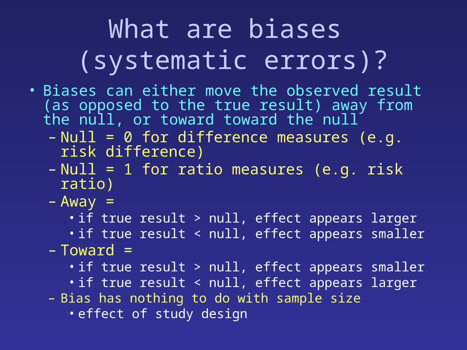
• Biases can either move the observed result (as opposed to the true result) away from the null, or toward toward the null– Null = 0 for difference measures (e.g. risk
difference) – Null = 1 for ratio measures (e.g. risk ratio)– Away =
• if true result > null, effect appears larger• if true result < null, effect appears smaller
– Toward =• if true result > null, effect appears smaller• if true result < null, effect appears larger
– Bias has nothing to do with sample size• effect of study design

Null True ValueB
True ValueA
+ ∞
+ ∞
- ∞
0
0
1
+ ∞
+ ∞
- ∞
0
0
1
ObservedValue A
ObservedValue B
ObservedValue B
ObservedValue A
Bias Away from Null
Bias Toward Null

8
Direction of Bias
• Often, the result of bias is unpredictable– Either toward or away from null
• In some circumstances we can predict the effect a bias– Usually toward the null
8

Types of Bias
• Only 3 types of bias!
– all studies
– regardless of study design
• The different study designs have ways of dealing with these biases – whether it’s done effectively determines how valid the study is

The 3 different types of biases
• Confounding
• Information Bias (Measurement Error)
• Selection Bias

11
Confounding

Confounding
• Question:
– Are there other factors that may account for the apparent relationship between exposure (intervention) and disease (outcome)?
– or
– Is there a common cause of both exposure and disease?
Observed Value2
Observed Value2
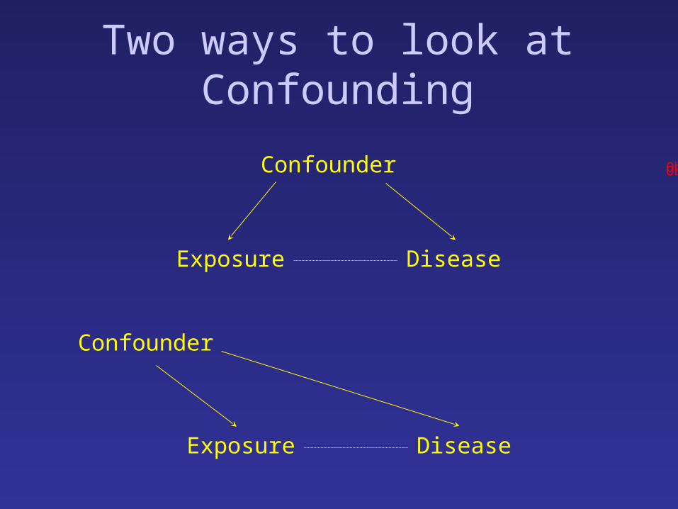
Exposure Disease
Confounder
Exposure Disease
Confounder
Two ways to look at Confounding

Confounding
• Note– Confounder not caused by exposure or disease– Confounder not on causal path from exposure
to disease• i.e. not an intermediate
Exposure Disease
Confounder

15
Examples
SSRI Suicide
Depression
CRP CAD
Diabetes
Yellow Finger Lung Cancer
Smoking

16
Why Does Confounding Occur?
• As an imbalance in proportions of the confounder between the two comparison groups
Total Population
Exposed Unexposed
No. of Cases 4,600 140
N 1,000,000 1,000,000
Risk 0.0046 0.00014
Risk Ratio 0.0046 / 0.00014 = 33

Men
Exposed Unexposed
Cases 4,500 50
N 900,000 100,000
Risk 0.005 0.0005
RR 10
Women
Exposed Unexposed
Cases 100 90
N 100,000 900,000
Rate 0.001 0.0001
RR 10
Total Population
Exposed Unexposed
Cases 4,600 140
N 1,000,000 1,000,000
Risk 0.0046 0.00014
RR 33

Total Population
Exposed Unexposed
Cases 4,600 140
N 1,000,000 1,000,000
Risk 0.0046 0.00014
RR 33
Men
Exposed Unexposed
Cases 4,140 14
N 900,000 100,000
Risk 0.0046 0.00014
RR 33
Women
Exposed Unexposed
Cases 460 126
N 100,000 900,000
Risk 0.0046 0.00014
RR 33

Total Population
Exposed Unexposed
Cases 3,500 350
N 1,000,000 1,000,000
Risk 0.0035 0.00035
RR 10
Men
Exposed Unexposed
Cases 2,500 250
N 500,000 500,000
Risk 0.005 0.0005
RR 10
Women
Exposed Unexposed
Cases 1,000 100
N 500,000 500,000
Risk 0.001 0.0001
RR 10

Why Does Confounding Occur?
Exposure Disease
Confounder
Men
Exposed Unexposed
Cases 4,500 50
N 900,000 100,000
Risk 0.005 0.0005
RR 10
Women
Exposed Unexposed
Cases 100 90
N 100,000 900,000
Rate 0.001 0.0001
RR 10

Why Does Confounding Occur?
Yellow Fingers Lung Cancer
Smoking
Smokers
Yellow Not Yellow
Cases 4,500 500
N 900,000 100,000
Risk 0.005 0.005
RR 1
Non-smokers
Yellow Not Yellow
Cases 100 900
N 100,000 900,000
Rate 0.001 0.001
RR 1Crude RR = (4,600/1M) / (1,400/1M) = 3.3

Confounding cont’d
• Does hyperlipidemia cause MIs?– Do higher lipid levels cause MIs?
High Lipids MI?
BP, age, gender, BMI, smoking, DM

– Does lowering lipid levels lower the risk of MI?
• Does statin use lower lipids?– If so, does that have an effect on lowering MI events?
statins lower lipid levels, MI?
BP, age, gender, BMI, smoking, DM, other healthy lifestyle factors, adherence

– Does a diet high in cholesterol increase the risk of MI?
• Does a ‘heart healthy diet’ lower lipids?– If so, does that have an effect on lowering MI events?
Healthy heart diet lower lipid levels, MI?
BP, age, gender, BMI, smoking, DM, other healthy
lifestyle factors, diet, exercise, adherence

Confounding by Indication
• Particularly common and difficult to deal with in (observational) pharmacoepidemiology studies
SSRI Suicide
Depression
TNF-antagonistuse
Lymphoma
RA diseaseseverity

What Confounding is NOT
• Confounding IS NOT– A factor on the causal pathway (intermediate)
• high fat diet LDL CAD• smoking adenomatous polyp colon CA
– A factor that modifies the relationship between an exposure and a disease
• Effect of anti-HTN drug is different in Blacks vs Whites
• Effect of blood levels of X on risk of Y in men vs women

Effect Modification(aka Interaction)
White Americans
High BP Normal BP
MI 4,500 50
N 900,000 100,000
Risk 0.005 0.0005
RR 10
Black Americans
High BP Normal BP
MI 200 90
N 100,000 900,000
Rate 0.002 0.0001
RR 20
Total Population
High BP Normal BP
MI 4,700 140
N 1,000,000 1,000,000
Risk 0.0047 0.00014
RR 33.6

How does a RCT addressConfounding?
• Randomization – evenly distribute both known and unknown
confounders (by chance) between the two (or more) exposure groups (i.e. active treatment and placebo)
– Can use specific inclusion/exclusion criteria to ensure everyone is the same for a particular confounder (e.g., all males in the study) [also known as restriction]

Control of Confounding by Randomization
– Since potential confounders are balanced between exposure groups, they can’t confound the association
Depression
SSRI placebo
Death 250 250
N 500,000 500,000
Risk 0.0005 0.0005
RR 1
No Depression
SSRI placebo
Death 100 100
N 500,000 500,000
Risk 0.0002 0.0002
RR 1
Suicide
Depression
SSRI
1,000,000 get SSRI1,000,000 get placebo
Depression distributed equally by chance, so:Crude RR = (350/1M) / (350/1) = 1

Control of Confounding in an RCT
1. Check Table 1 for imbalances between treatment arms
– Are any of the differences clinically meaningful? (not the same as statistically significant!)
– How could those differences affect the results?– What other potential confounders are missing
from Table 1?– Could they affect the results if they were
imbalanced between the treatment arms?– How likely is it that unknown confounders are
imbalanced? (with large RCTs, unlikely)

Control of Confounding in a RCT
2. Intention-to-treat analysis
– Maintains the balance of potential confounders given by randomization, thereby continuing to (theoretically) address confounding
– May need to ‘control’ for very unbalanced factors in the analyses

Control of Confounding in Observational Studies
• Study design level: Restriction– Inclusion/exclusion criteria to limit study population to a more
homogeneous group• E.g. study of alcohol and MI may exclude smokers since smoking is
an important confounder
• Data analysis level: Stratification– Analyze data stratified by an important confounder
• E.g. evaluate effect of alcohol on MI among smokers and among non-smokers separately
• Added advantage: identifies effect modification
• Data analysis level: Regression– ‘Control’ for potential confounders in regression models
• can also identify effect modification if planned for by investigators
• Matching– Match on potential confounding variables

33
Control of Confounding in Observational Studies
1. Have the investigators identified all the important potential confounders in the study?– What factors could be common causes of
both exposure and disease?
2. Have the investigators accounted for these potential confounders either in the design of the study or in the analysis?
3. If they haven’t, how might that affect the results they found? 33
34
Confounding: Examples

35
• In large RCTs, confounding is not usually an important issue– Randomization distributes confounders
equally between trial arms
• Table 1 appears to confirm this– Probable confounders seem to be well
balanced35

36
Is this difference important? Previous fractures are a risk for future fractures ...

37
• Questions to ask:1.What are the potential sources of confounding?
2.Have the authors identified these potential confounders
3. How have the authors addressed potential confounders?
4. Was this sufficient?

38
1. What are the potential sources of confounding?
• Risk factors for exposure– i.e. for NSAID use
• RA? (chronic NSAIDs)• CAD prevention? (ASA)• prior GI bleeding? (avoid NSAIDs, use coxib)• age? (avoid NSAIDs)
confounder
NSAIDor type of NSAID
CV event
• Are any of these also related to the likelihood of having an event?
38

39
1. What are the potential sources of confounding?
• Risk factors for outcome?– i.e. having a CV event
• smoking?• prior CV event?• general health?• ASA use? (preventative)• age?
confounder
NSAIDor type of NSAID
CV event
• Are any of these also related to the likelihood of being exposed to an NSAID or type of NSAID?
39

40
• Confounding by indication– Almost always a concern in observational studies of
drugs– Here, could the reason that NSAIDs are prescribed (the
‘indication’) be related to both exposure (NSAID prescription) and disease (CV outcomes)?
– What about reasons to avoid NSAIDs?• Chronic kidney disease?• Other health problems?
1. What are the potential sources of confounding?
pain
NSAIDor type of NSAID
CV event
CKD
NSAIDor type of NSAID
CV event
Poor health
NSAIDor type of NSAID
CV event

41
2. Have the authors identified these potential confounders?
• In this study, seems like yes– they even have a section talking about
‘covariates’

42
3. How have the authors addressed potential confounders?
• Statistical analysis, • ‘Advanced methods’
43
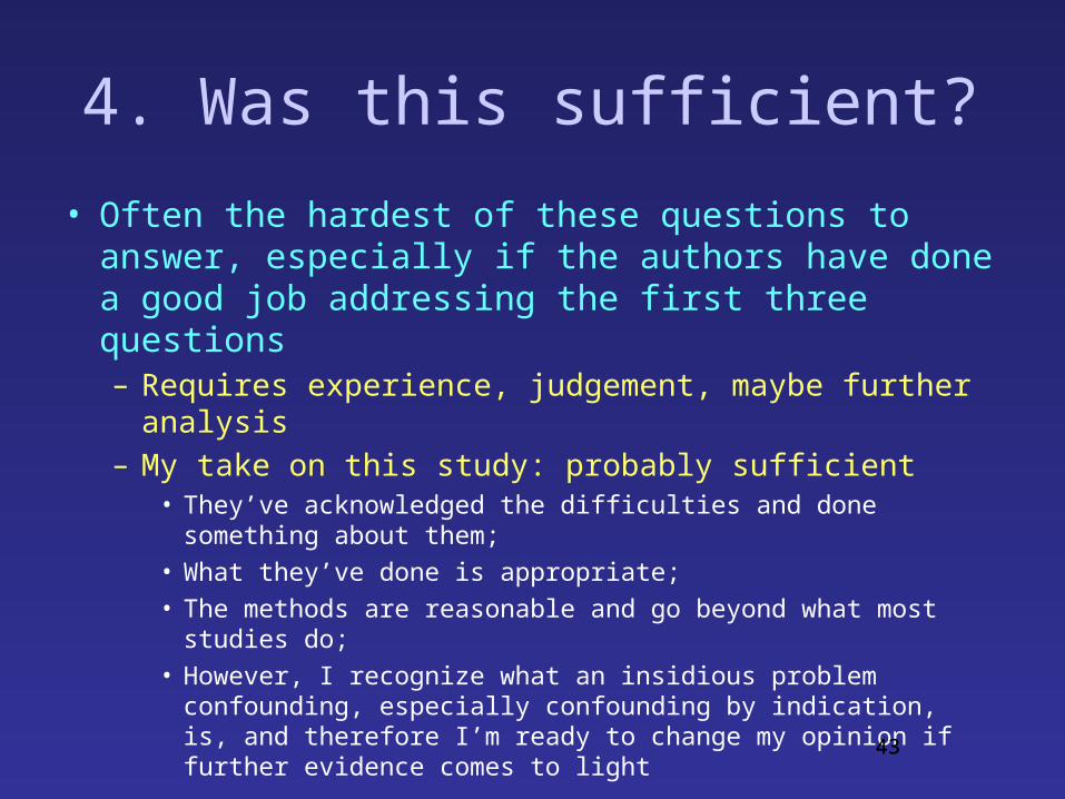
4. Was this sufficient?
• Often the hardest of these questions to answer, especially if the authors have done a good job addressing the first three questions– Requires experience, judgement, maybe further
analysis– My take on this study: probably sufficient
• They’ve acknowledged the difficulties and done something about them;
• What they’ve done is appropriate;
• The methods are reasonable and go beyond what most studies do;
• However, I recognize what an insidious problem confounding, especially confounding by indication, is, and therefore I’m ready to change my opinion if further evidence comes to light43

44
• Questions to ask:1. What are the potential sources of confounding?
2. Have the authors identified these potential confounders?
3. How have the authors addressed potential confounders?
4. Was this sufficient?

45
• This is another pharmacoepidemiologic study (kind of), so let’s jump right to confounding by indication again– Here, could the reason that DMARDs were prescribed (the
‘indication’) be related to both exposure (DMARD use) and disease (lymphoma)?
• -> Disease severity, i.e. chronic inflammation
1. What are the potential sources of confounding?
disease severity
DMARDor type of DMARD
lymphoma

46
2. Have the authors identified these potential confounders?– Clearly - that is what this paper is all about

47
3. How have the authors addressed potential confounders?
• Here:– detailed assessment of disease severity for
each subject– mutual control of drug use and disease severity
etc.

48
4. Was this sufficient?
• Again, this is often the hardest of these questions to answer,– My take on this study: probably sufficient
• They’ve acknowledged the difficulties and done something about them;
• What they’ve done is appropriate;• The methods are reasonable;• Again though, I recognize what an insidious
problem confounding, especially confounding by indication, is, and therefore I’m ready to change my opinion if further evidence comes to light
48

49
Information Bias(Misclassification)

Information Bias
• Could exposure (intervention) or disease (outcome) be inaccurately reported or measured
– i.e. misclassified?

Information Bias
• Information about exposure, disease, and/or confounder(s) is erroneous– Misclassified into the wrong category
True exposure True disease status
Measured exposure Measured disease status

Examples of Information BiasTrue EtOH
Reported EtOH Fetal outcome
True illicit drug use True blackouts
Reported illicit drug use Reported blackouts
True Gastritis status
Drug Gastritis by chart review
Exposure misclassification
Outcome misclassification
BOTH exposure and outcome misclassification
If using the same source for exposure and disease information (e.g., from the participant), can get very biased results
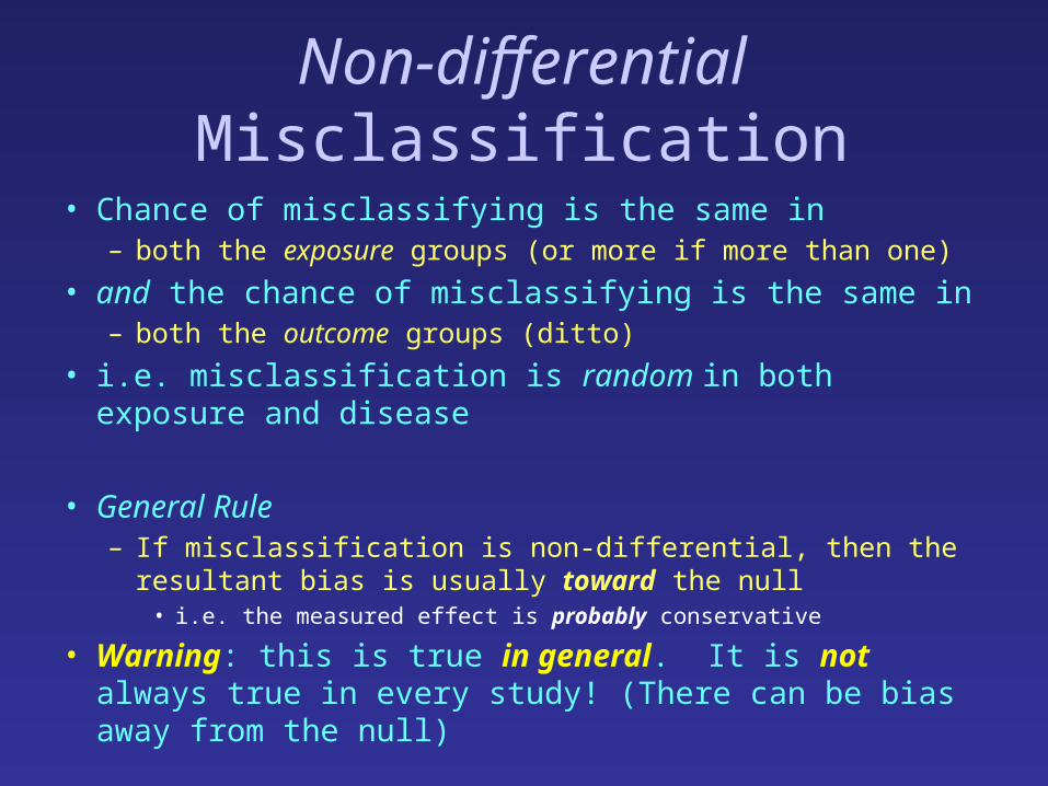
Non-differential Misclassification
• Chance of misclassifying is the same in– both the exposure groups (or more if more than one)
• and the chance of misclassifying is the same in– both the outcome groups (ditto)
• i.e. misclassification is random in both exposure and disease
• General Rule– If misclassification is non-differential, then the resultant
bias is usually toward the null• i.e. the measured effect is probably conservative
• Warning: this is true in general. It is not always true in every study! (There can be bias away from the null)

Differential Misclassification
• Chance of misclassifying is not the same in either– the two exposure groups (or more if more than one)
• or
– the two outcome groups (ditto)
• i.e. misclassification is not random in either exposure or disease
• In this case, the resultant bias is unpredictable!– Consider carefully whether you think any
misclassification is likely to be differential or non-differential!

How does an RCT addressInformation Bias
• EXPOSURE:– Exposure is assigned (randomly) in an RCT
• the label of the treatment arm is a proxy for the actual exposure
• bias is usually non-differential
Assigned exposure
Actual exposure Outcome

56
How does an RCT addressInformation Bias
• EXPOSURE:– Problems: non-adherence and contamination
• With less than 100% adherence, intention-to-treat analysis is biased due to information bias (usually non-differential)
• If using a ‘completers’ analysis (only analyze those completing the study in their assigned group), information bias is addressed, but
• introduces confounding and selection bias (when subjects leave the study)
– randomization has been broken– reasons for withdrawal could be related to treatment
» TRUTH is somewhere between ITT and completers analysis when <100% adherence (almost always)
56

57
Treatment A
Treatment B
• ITT - thought to be more conservative estimate• (biased toward null)
• Completers analysis - thought to usually exaggerate estimate

Information Bias in an RCT
• OUTCOME• allocation concealment (nobody knows what the next
treatment assignment will be)• blinding (investigators and subjects)• same study procedures for all arms
– these should prevent non-differential misclassification of the outcome
• any bias should be toward the null
– Problems:• Unblinding (e.g. side effects from treatment)• Accuracy of outcome assessment
– reliability, reproducibility

Information Bias in Observational Studies
• Obtain information about exposure and outcome in a structured manner (preferably ‘objective’ sources)– Obtain information about the disease in exactly the
same fashion regardless of the exposure status– Obtain information about the exposure in exactly the
same fashion regardless of the disease status– Use different sources of information for exposure and
disease if possible• If you ask someone about their alcohol use and also
ask them about how many times they fell, you are likely to get very skewed data
– EtOH users less likely to report both use and falls

60
Information Bias: Examples

61

62
Exposure misclassification?
• An RCT, so exposure should be random• Pill counts and interviews to assess whether
subjects took medications as assigned• Not an ITT (but not a completers analysis either)
– (the method they used is probably better than an ITT analysis - you’ll just have to trust me)

Outcome misclassification?
• Allocation concealment– Not commented upon
• unfortunately this is common
• we’ll presume allocation was concealed
• Blinding– Stated to be double-blind
• placebos for both interventions (blinds subjects in absence of noticeable side effects)
• BMD scan results withheld from local investigators (blinds investigators)
• Outcome assessments– BMD - ‘Quality assurance, cross-calibration adjustment, and data
processing were done centrally’• presumably without knowledge of treatment assignment
– Fracture - ‘Radiographs were assessed in a blinded fashion by an independent reader’
• presumably using a standard protocol of some kind

64
Likelihood of Information Bias
• Appears to be minimal
• Any bias should be toward the null
• Estimates therefore likely to be conservative (underestimate true results)
64

65

Exposure misclassification?
1. How was exposure assessed?– prescriptions for NSAIDs (including coxibs)
2. Could exposure be mis-measured?– here, a prescription does not guarantee that the subject
actually took the medication, or that s/he took it as prescribed
– OTC medication use may not be measured
NSAID use
NSAID Prescription CV event

Exposure misclassification?
3. Is any exposure mis-measurement likely to be non-differential or differential?– Three questions here:
1. Coxibs vs traditional NSAIDs
2. NSAIDs vs comparison meds (glaucoma/thryoid meds)
3. Are chronic NSAID users likely to differ in their ‘compliance’ compared to glaucoma/thyroid med users (or coxib users)?
1. Some traditional NSAIDs are available OTC• coxibs are not• therefore, more likely that NSAID use is mis-measured
(underestimated)• therefore, differential misclassification is likely
2. Same potential problem with NSAIDS in general (some available OTC) and comparison meds (prescription needed)

68
Exposure misclassification?
3. Is any exposure mis-measurement likely to be non-differential or differential?3. Are chronic NSAID users likely to differ in
their ‘compliance’ compared to glaucoma/thyroid med users (or coxib users)?• I’m not sure but I suspect there might be a
difference.
• Any opinions?
68

Outcome misclassification?
1. How was outcome assessed?– CV outcomes based on various codes in admin
records
2. Could exposure be mis-measured?– errors made by coders (doctors, administrators, etc.)– no verification that a coded event is an actual event
Codes for CV events
NSAID Prescription CV event

Outcome misclassification?
3.Is any outcome mis-measurement likely to be non-differential or differential• Is it more likely for persons not coded with a CV
event to actually have a CV event?• or for persons coded with a CV event to not have
one?
• Or does each seem equally likely?
• To me, I think it’s more likely that persons coded for a CV event were mis-coded compared to persons who never received a code in the first place.

Likelihood of Information Bias
• Overall, low-moderate
• Likelihood of differential misclassification is moderate
• I recognize this risk, think the authors are also aware of it and have considered it, and conditionally accept the results of the study pending further studies

72

Exposure misclassification?
1.How was exposure assessed?• Exposure here is degree of inflammation
• Apparently, standardized, protocolized assessment of tender/swollen joints
2.Could exposure be mis-measured?– Physician error in counting joints
Tender/swollen joint count
Inflammation Lymphoma

Exposure misclassification?
3.Is any exposure mis-measurement likely to be non-differential or differential?• Not 100% sure, but seems to me like it’s likely
to be non-differential• i.e. all patients have RA
• More likely to count more joints if subject seems more ‘active’?
• Less likely to count more joints if subject seems to be doing subjectively well?

Outcome misclassification?
1. How was outcome assessed?– Cases - occurrence of lymphoma– All cases validated and confirmed– Controls - random other RA subjects w/o RA
2. Could exposure be mis-measured?– Would have to argue that some of those without lymphoma
actually had missed cases - seems unlikely
Lymphoma on biopsy
Inflammation Lymphoma

Outcome misclassification?
3.Is any outcome mis-measurement likely to be non-differential or differential• As said, risk seems small but any risk would
have to be non-differential• Cases are almost certainly lymphoma
• Could be some controls who actually should be cases

Likelihood of Information Bias
• Overall, low
• Likelihood of differential misclassification is also low
• Effort taken to verify cases and relatively rarity of lymphoma in those who are controls virtually eliminates the risk of information bias in this study.

78
Selection Bias

Selection Bias
• Is study entry or exit related to exposure (intervention) or disease (outcome)?

Selection Bias
• Factors that influence study participation– Subjects entering and staying in the study
• exposure-disease association is different among those who participate than among those who do not– E.g. healthy worker effect

Exposure
Disease
Participation
New Drug
Pain
Those who completed study
Example of Selection Bias
DM
Gall bladder
Hospitalized patient
Chemical
Lung disease
Healthy worker
(compared to general
population)
Lipids
MI
Health conscious or familial hypercholesterolemia or other high risk

How does an RCT address Selection Bias?
• Study entry: Randomization after study entry prevents any factors related to the exposure from influencing study participation

How does a RCT address Selection Bias?
• Study exit: Try to achieve full follow-up– Problem: Loss-to-follow-up (LTFU)
• LTFU is almost always related to either the exposure or disease or both (e.g. drug is ineffective (outcome), or drug has side effects (exposure))
• Equal numbers of LTFU in treatment arms does not guarantee that the there is no selection bias (different reasons for dropout)
• Analytic techniques such as last observation carried forward or multiple imputations do not “take care of” selection bias

Selection Bias in Observational Studies
• Difficult to deal with selection bias in observational studies– Can’t always control factors influencing study
participation• Healthy worker effect: use a group in the same
office/factory not exposed to the particular chemical
– Try to minimize loss-to-follow-up• Use appropriate analytic methods to account for
differing lengths of follow-up (incidence rate ratio, hazard ratio)

‘Representativeness’:This is NOT a bias
• Trying to make one’s study population ‘representative’ of a more general population is counter to using restriction for control of confounding– Basic science animal studies ‘restrict’ study population to
genetically homogeneous lab animals• To elaborate a scientific theory about a biologic process
• If a different group is of clinical interest, should conduct well-designed study in that group to determine whether effects differ in that group– This is a question of whether the BIOLOGY is different in that
group• This is an issue of “Effect Measure Modification”

86
Selection Bias: Examples

87

88
A Clinical Trial
• Selection bias due to study entry is virtually never an issue– true here– patients randomized after selection for study
• Loss to follow-up– 70 (33%!) in alendronate group– 64 (30%!) in teriparatide group– These are fairly high rates of LTFU!
88
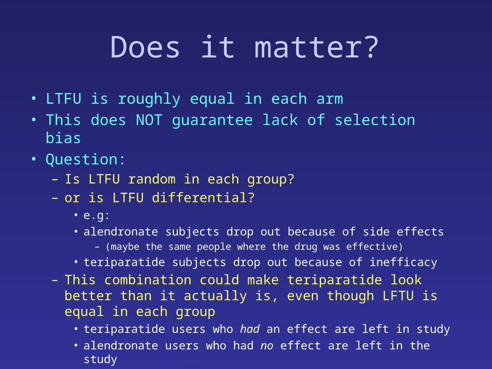
Does it matter?
• LTFU is roughly equal in each arm• This does NOT guarantee lack of selection bias• Question:
– Is LTFU random in each group?– or is LTFU differential?
• e.g:• alendronate subjects drop out because of side effects
– (maybe the same people where the drug was effective)
• teriparatide subjects drop out because of inefficacy
– This combination could make teriparatide look better than it actually is, even though LFTU is equal in each group
• teriparatide users who had an effect are left in study• alendronate users who had no effect are left in the study

90
Judgement
• Seems to me that drop out is likely to be random
• above scenario is unlikely
– Therefore I doubt there is much if any selection bias in this study
90

91

92
Study entry
• The authors recognize that healthy people are less likely to have records in their study database– one reason they used other drug-users
(glaucoma and hypothyroid) as a control group
• Therefore healthy persons may be less likely to be selected as a comparison group subject– disease estimate in control group could be
exaggerated– results in underestimate of true risk
92

93
Study exit
• Subjects could leave study if they got insurance, e.g.– are persons who did this more likely to be
NSAID users? or to have an event? or both?– are healthier persons more likely to get
insurance and not have an event?• I would think so• leaves less healthy persons who could have an
event in the control group– more events in control group– underestimate true risk 93

94
Judgement
• Selection bias is certainly possible– Recognized by authors– Methods to minimize (drug using control
group)
• Overall, risk is there but is probably not very high(?)
94

95

96
Study entry
• Entry in this study is based on case-control status
• How could cases or controls be unrepresentative of RA patients?
• All RA patients should have been captured in this RA registry
• All lymphoma patients should also be captured in the lymphoma registry
• One reason why ‘population-based’ studies are nice!
96

97
Study exit
• As with entry, these registers should capture all RA patients who have had lymphoma
• If RA patients left the study before they got lymphoma that could be a source of bias
• But these persons could not have been cases or controls.
• Again, likelihood of selection bias seems low
97

98
Judgement
• Selection bias seems unlikely in this nested case-control study
• Note, this can often be the case in c-c studies where the underlying population is well-defined (esp. population-based studies)
• When this is NOT the case (e.g. hospital-based c-c study) selection bias is much more likely
98

Interpreting Study Results
• Any study’s results must be interpreted in the context of whether or not there are any biases that could have deviated those results from being the truth– This is the critical step in understanding
whether or not these results are clinically meaningful for your patients – i.e., are the results valid?
• If there are biases, you need to try to determine how much they would have affected the results – would the message still be about the same even taking those biases into account?

Summary
• You should now be able to:– Understand that all study designs use various
strategies to address systematic error (bias) to varying degrees of success
– Understand how to identify confounding, information bias, selection bias

101
Random Error

Goals
• Review random error (statistical precision)– Review the correct interpretations of
confidence intervals and p-values– Review Type 1 and Type 2 errors

Random Error vs Systematic Error
Study size
Mea
sure
d va
lue
True value
Syst error
Random error
In absence of bias, with perfect precision

Random Error
• Results from variability in the data, sampling– E.g. measuring height with measuring tape: 1
measurement may be off, but multiple measurements will give you a better estimate of height
• Relates to precision• We use confidence intervals to express the
degree of uncertainty/random error associated with a point estimate (e.g. a RR or OR)– Measure of precision

Confidence Interval
• Epidemiologist/biostatisticians have arbitrarily chosen 95% as the level of confidence to report
• 95% C.I.=if the data collection and analysis were repeated infinitely, the confidence interval should include within it the correct value of the point estimate 95% of the time– Note: this is NOT the same as saying the confidence
interval is 95% likely to contain the ‘true’ value. (INCORRECT!!)
– ASSUMES NO BIAS

True value for RR
90% confidence intervals from repeated studies

Confidence Interval cont’d
• If the confidence interval includes the null (‘1’ for relative measures of effect (e.g. RR, OR), ‘0’ for absolute measures of effect (e.g. risk difference)), the result is considered to be not statistically significant– Since the CI contains the correct value 95%
of the time, the correct value could be the null

Confidence Interval cont’d
• “Precision” relates to the width of the confidence interval– A very precise estimate of effect will have a
narrow CI– Can improve precision by:
• Increasing sample size

P-value
• The P-value is calculated from the same equations that lead to a confidence interval
• Again, 0.05 (related to the 95% CI) was arbitrarily chosen
• P-values are confounded by magnitude of effect and sample size (precision)– Can get a very small p-value if a study is
large enough, even if the effect is very small

P-value
• P-value=assuming the null hypothesis is true, the p-value is the probability of this result or one more extreme, assuming no bias/confounding– E.g. RR=2, p=0.03: “Assuming the null hypothesis is
true (RR=1), the probability of this result (i.e. RR=2) or one more extreme (i.e. RR>2) is 3%”
– E.g. RR=0.4, p<0.001: “Assuming that there truly is no difference between the two treatment groups, the probability of obtaining a RR of 0.4 or one more extreme (i.e. RR<0.4) is less than 0.1%”

• Note: this is NOT the same as saying the p-value is the probability that the null hypothesis is true (INCORRECT!! since it is conditioned on the null being true) – Just because your p-value isn’t “statistically
significant” doesn’t mean that you can say the two arms are “equivalent”
• The p-value says nothing about the probability of your alternative hypothesis being true
• Think of the p-value as a relative marker of how consistent the data are with the null hypothesis

Statistical Significance Testing• Statistical significance testing is really only
about statistical precision– How precise are the study results?– P-values on their own tell you NOTHING about the
magnitude of effect; 95% CI confidence intervals at least give you an idea of potential magnitude of effect
– P-values and 95% CI tell you NOTHING about how valid the results are (i.e., whether the results are biased)
• We should place LESS emphasis on statistical significance and rather think MORE about clinical significance or meaningfulness when considering the results and validity of a study

Type I, Type II Errors
• Emanating from α=0.05, Type I error is made if one incorrectly rejects the null hypothesis when the null hypothesis is actually true– This probability is determined by the
significance level alpha (=0.05)
• Type II error is made if one fails to reject the null hypothesis when the null is false– This probability is determined by β, where 1-β
is the power, which is usually set at 80%

Basic Approach to Understanding Power
• Power calculations/sample size calculations:– Use estimate of the expected event rate in
the unexposed (placebo group)• Based on published literature/experience (e.g.,
10% of men age 60-70 have MIs)
– Based on that ‘background rate’, determine sample size needed to detect a difference of a specified magnitude between treatment and placebo with 80% power and alpha=0.05

115
Random Error: Examples

116

Statistical Significance: p-value given, but no confidence interval regarding the difference in means (i.e. the 95% CI for the mean BMD difference of 3.8%)
Can theoretically use the standard error (S.E.) information to calculate the 95% confidence interval
Adequate power? Sample size: 214/armHad sufficient power to detect 2% differencein BMD at L-spine (found 3.8% difference)
118

Statistical Significance
• 95% confidence interval given for each rate ratio
• Adequate sample sizes?– N=several thousand
persons for each drug– 100s-1000s of events– Null results (lack of
association) for some drugs is unlikely due to inadequate power (and did find association for Vioxx, as expected)
– ? Type 2 error
120

Statistical Significance
95% Confidence Intervals given for each Odds Ratio
Adequate sample size? 378 cases, 378 controls
They found an association, so no concerns about inadequate power due to insufficient sample size
? Type 1 error? Bias

Summary
• You should now be able to:– Understand that confidence intervals reflect
precision, which is related to sample size– Understand the correct interpretation of
confidence intervals and p-values– Understand that power relates to sample size