Embed Size (px)
Citation preview
Epipolar Constraints for Vision-AidedInertial Navigation
David D. DielMassachusetts Institute of Technology
Email: [email protected]
Paul DeBitettoDraper Laboratory
Email: [email protected]
Seth TellerMassachusetts Institute of Technology
Email: [email protected]
Abstract— This paper describes a new method to improveinertial navigation using feature-based constraints from oneor more video cameras. The proposed method lengthens theperiod of time during which a human or vehicle can navigatein GPS-deprived environments. Our approach integrates wellwith existing navigation systems, because we invoke generalsensor models that represent a wide range of available hard-ware. The inertial model includes errors in bias, scale, andrandom walk. Any purely projective camera and trackingalgorithm may be used, as long as the tracking output canbe expressed as ray vectors extending from known locationson the sensor body.
A modified linear Kalman filter performs the data fusion.Unlike traditional SLAM, our state vector contains onlyinertial sensor errors related to position. This choice allowsuncertainty to be properly represented by a covariance matrix.We do not augment the state with feature coordinates. Instead,image data contributes stochastic epipolar constraintsovera broad baseline in time and space, resulting in improvedobservability of the IMU error states. The constraints lead toa relative residual and associated relative covariance, definedpartly by the state history. Navigation results are presentedusing high-quality synthetic data and real fisheye imagery.
I. NAVIGATION PROBLEM
An Inertial Measurement Unit (IMU) is a common com-ponent in modern navigation systems. A typical IMU con-tains three accelerometers and three gyroscopes that provideinformation about the motion of a moving body [1]. Unfor-tunately, the process of extracting body position estimatesfrom IMU output leads to significant drift over time. TheGlobal Positioning System (GPS) provides complementary,absolute position information. However, circumstances suchas sky occlusion, hardware failure, and war may disallowGPS signals. Therefore, we turn to vision as an alternativesource of information.
We would like to navigate in places where people go onfoot or in a wheeled vehicle. Examples include warehouses,factories, offices, homes, city streets, suburbs, highways,rural areas, forests, and caves. These environments happen toshare some important visual characteristics: 1) Most of thescene remains stationary with respect to the planet’s surface;and 2) For typical scenes, the ratio of body velocity to scenedepth lies within a limited range. Other environments thatmeet these criteria include the sea floor and unexplored
Variables
t - timeyij - pixel radianceε - relatively small numberτ - interval of time (fixed)bbb - biascccij - camera rayfff - specific forceggg - gravityhhh - measurement gainkkk - Kalman gainnnn - white noisesss - scaleuuuij - image coordinatexxx - body statezzz - feature rayθθθ - Euler angles
ρρρ - imaging parametersRRR - rotation matrixΛΛΛ - covariance matrixΦΦΦ - transition matrix
Other Notation
�T - translation part�R - rotation part�T - transpose� - 1st temporal derivative� - 2nd temporal derivative~� - unit magnitude� - contains error� - residual� - estimated∆� - changeδ� - error�[ ] - discrete samples
Fig. 1. Symbols and notation. Scalars are regular italic; vectors are boldlowercase; and matrices are bold uppercase. Variables may vary with timeunless noted. The� symbol is a placeholder and subscriptsij indicateassociation with an array.
planets. The sky, outer space, and most seascapes do notfall in this category.
The goal of navigation is to find the transformationsxxx [t]that relate camera poses to a static reference frame. In avision-only context, Chiuso et al. have developed a causal(history-based), real-time algorithm to solve for3D relativescene geometry, while addressing scale ambiguity [2]. Mostof their discussion applies here, but we utilize the knowncharacteristics of an inertial sensor in our development. In-stead of tackling the Structure From Motion (SFM) problemdirectly, we aim to navigate first and leave scene geometryto be calculated later.
There exists a critical difference between self-localizationand relative target seeking. When the goal is relative po-sitioning for grasping, assembly, or impact, a convergentsolution can be derived [3]. A visible target needs no ab-solute reference frame. However, if we want geo-referencednavigation coordinates in the absence of landmarks, then our
sensor combination will face performance limitations. Theonly source of absolute position information is the planetarygravity potential, and this potential is ambiguous over eachiso-layer (the ocean surface is one of them). In essence,the system we have described cannot converge to the actualtrajectory. So, we will present atransientsolution that aimsto reduce drift.
II. A PPROACH
Several ideas from machine vision have potential rele-vance to inertial navigation. The list would certainly includestereo vision, optical flow, pattern recognition, and trackingof points, curves, and regions. Each of these methodsproduce a different kind of information. Stereo vision mayproduce dense relative depth estimates within a limitedrange. Optical flow can produce dense motion fields. Patternrecognition can locate the direction to a unique landmark,which may be linked to absolute coordinates. And finally,tracking can offer data association over multiple frames.
The scope of relevance can be limited by consideringsystem requirements and constraints. We want an automaticmethod that is robust to visual distractions such as occlu-sion, variation in lighting, and ambiguities. It should workwith one or more cameras, within reasonable computationallimits, given no prior knowledge of the environment. Thesechoices bring the focus to either flow-based or tracking-based approaches.
A. Tracking vs. Flow
Both optical flow and tracking provide local estimates ofimage motion. As a camera translates, light rays from theenvironment slice through a theoretical unit sphere centeredat the camera’s focus. Patterns of light appear to flowoutward from a point source, around the sides of the sphere,and into a drain at the opposite pole. If the camera alsorotates, then a vortex-like flow is superimposed on the flowinduced by translation. Despite the naming conventions,both optical flow and tracking are supposed to track theflow. The difference between them lies in the selection ofdiscrete coordinates. Optical flow calculations are defined ona discrete regular mesh, with the assumption of underlyingspatial and temporal continuity. Tracking methods tend toutilize discrete particles that retain their identity over a broadbaseline in time.
Our method tracks sparse independent corner features forthe following reasons: 1) To avoid the texture ambiguityassociated with optical flow; 2) To gain leverage against theaccumulation of inertial drift over time; 3) To facilitate de-tection of visual distractions; and 4) To bound computationalrequirements.
By appealing to feature tracking in general, most as-sumptions about the visual context can be avoided. Forexample, one could use infrared imagery to handle low
light conditions. Landmarks such as corporate logos andbarcodes may provide useful information when they areavailable, but none are required. Mixed resolutions anddropped frames are also handled. The only requirements area static electromagnetic environment and sensors selectiveto an appropriate frequency band.
B. Data Fusion
Probably the most common approach to combining fea-ture observations with inertial data is Simultaneous Local-ization and Mapping (SLAM) [4][5][6]. SLAM takes onthe burden of mapping and the computational complexityof map maintenance in exchange for maximal informationusage. Nearly all SLAM solutions are based on the ExtendedKalman Filter (EKF) [7], which scales quadratically withthe number of states. Extensions such asAtlas [8] andFast-SLAM [9] have been developed to manage large maps, butthe benefits of mapping may not justify the computationalcost. Furthermore, the EKF may be far from optimal due toits linear approximations.
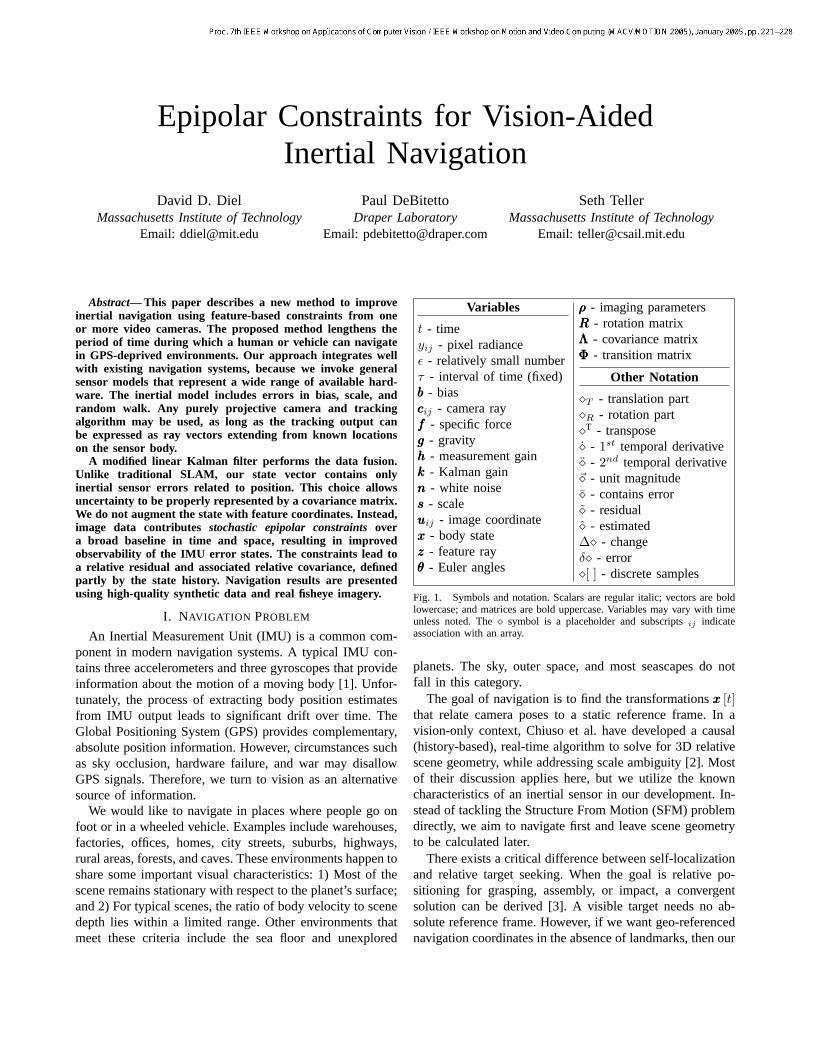
Fig. 2. Proposed block diagram showing sensor fusion in the EPC Filter.
Our approach toward data fusion focuses on the inter-pretation of visual measurements. As in other methods, wepropagate the IMU error state, apply visual updates, andremove translation error. Uncertainty is represented by acovariance matrix. However, our filter does not maintainstates for each feature, but instead treats visual measure-ments as independentstochastic constraintson the cameraposition. Specifically, out-of-plane violations of the epipolarconstraint (EPC) are fed into a linear Kalman filter asprojected residuals. By disregarding in-plane information,the measurement equation avoids explicit dependency onscene depth. In this framework, computation and memoryrequirements scale linearly with the number of visiblefeatures. For related work in vision-only navigation, see[10][11][12].
C. Gyroscope Reliance
Modern gyroscopes (gyros) can be trusted to provideaccurate orientation estimates for periods up to several min-utes [13]. For some hardware combinations, gyro accuracyexceeds imaging accuracy by orders of magnitude. Considera typical wide-field video camera with a pixel separation of0.25 degrees. A common flight control gyro can maintainsimilar angular precision for about10 minutes with novisual assistance. Thus, our method relies on the gyros tocompensate for camera rotation, but image data is not usedto improve the gyros.
III. IMU D EFINITION
We begin with a simplified strapdown1 inertial sensormodel in a static North-East-Down (NED) visual frame. Astrapdown IMU is designed to measure specific force andorientation changes in its own body frame. We assume idealgyros, and noisy accelerometers, as described in SectionII. The gyros output small changes∆θθθ [t], which can beintegrated to find an associated direction cosine matrixRRR (t).The visual frame moves with the planet, so the planetaryrotation rate should be subtracted from the gyro outputduring integration. The accelerometers measure a non-trivialcombination of acceleration and gravitation.
fff = RRR−1 (xxxT − gggapp
)(1)
Note the apparent gravitation term, which has an approx-imate value of9.8 m
s2 near the Earth’s surface. To gainmore significant digits, planetary rotation effects in the NEDframe must be taken into account. These effects dependstrongly on latitude and altitude, and weakly on velocity.We use the gradient of the second-order spherical harmonicdefined in WGS84 to model Earth’s gravitational field[14][15], and add higher-order terms when they are justifiedby the sensor accuracy.
Assuming the apparent gravity model accuracy exceedsthat of our accelerometers, the primary sources of measure-ment error are bias, scale and random walk.
fff = (III + diag(δsss))fff + δbbb+nnnw (2)
Rewriting as an acceleration measurement yields
¨xxxT = RfRfRf + gggapp
=(xxxT − gggapp
)+RRR (diag(δsss)fff + δbbb+nnnw) + gggapp
= xxxT +RRRdiag(fff) δsss+RRRδbbb+nnnw
(3)Therefore, omitting the second order effect of diag(δfff) δsss,the error process may be defined
δxxxT ≡ ¨xxxT − xxxT = RRRdiag(fff)δsss+RRRδbbb+nnnw (4)
which leads to a Linear-Time-Varying (LTV) state-spacemodel for the translation error. Note the nonlinearity with
1Similar equations can be derived for a gimballed IMU.
respect to external inputsRRR and fff , though no elements ofψψψ appear inΦΦΦ:
ψψψ = ΦΦΦψψψ +nnn (5)
ψψψ ≡
δxxxT
δxxxT
δbbbTurnOn
δbbbInRun
δsssTurnOn
δsssInRun
nnn =
000nnnw
000nnnb
000nnns
ΦΦΦ =
000 III 000 000 000 000000 000 RRR RRR RRRdiag
(fff)
RRRdiag(fff)
000 000 000 000 000 000000 000 000 − III
τb000 000
000 000 000 000 000 000000 000 000 000 000 − III
τs
To calculate the body position without image data,
one would twice integrate the first form of Equation 3.Given image data, one would also integrate the statespace and apply stochastic updates yet to be defined. Inour discrete-time implementation, we use the following:
ψψψ [t] = expm(τΦΦΦ [t− τ ])ψψψ [t− τ ]
ΛΛΛ [t] = expm(τΦΦΦ [t− τ ])ΛΛΛ [t− τ ] expm(τΦΦΦ [t− τ ])T + ΛΛΛn
(6)where τ is a small time step, typically in the range of10 to 400 Hz. Here, expm( ) represents the matrixexponential function. The driving noise is zero meanGaussian, uncorrelated with itself over time. Therefore, itsfirst order expectation is zero E[nnn] = 000, and its secondorder expectation is the diagonal matrixΛΛΛn = E
[nnnnnnT
].
IV. CAMERAS AND TRACKING
This section describes one way of sampling the space oflight rays surrounding a moving body. Any optical systemthat produces ray-based observations from known relativevantage points may be used. For example, the system mightconsist of multiple active cameras attached to the body bykinematic linkages. However, for clarity, the discussion willbe limited to one calibrated camera having a single focusconcentric with the IMU’s inertial axes2.
A. Camera Definition
A calibrated camera can be defined by its transformationfrom the space of light rays to the image space [16]. Tocalculate an image coordinate, a ray in the world frame isrotated into the camera frame~c~c~c = RRR−1~z~z~z and projected tothe image spaceuuucam = uuucam (~c~c~c), whereuuucam ∈ [−111 111]stretches-to-fill a square array. A forward-right-down frameis associated with the camera, such that~c~c~c = [1 0 0]T
corresponds to the optical axis.
2In an extended development, camera offset would appear in Equation10, and body-relative camera rotation would appear in Equation 7.
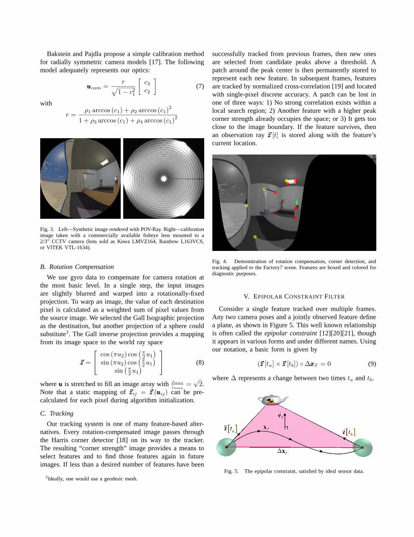
Bakstein and Pajdla propose a simple calibration methodfor radially symmetric camera models [17]. The followingmodel adequately represents our optics:
uuucam =r√
1− c21
[c3c2
](7)
with
r =ρ1 arccos (c1) + ρ2 arccos (c1)
2
1 + ρ3 arccos (c1) + ρ4 arccos (c1)2
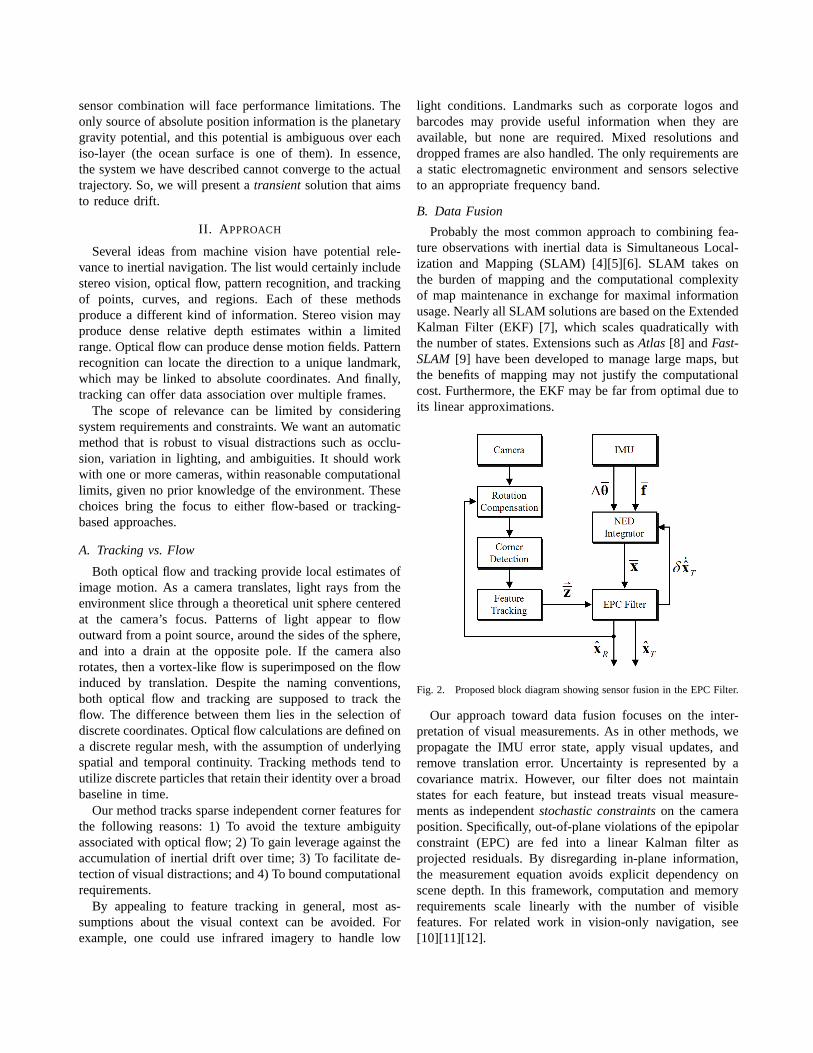
Fig. 3. Left—Synthetic image rendered with POV-Ray. Right—calibrationimage taken with a commercially available fisheye lens mounted to a2/3” CCTV camera (lens sold as Kowa LMVZ164, Rainbow L163VCS,or VITEK VTL-1634).
B. Rotation Compensation
We use gyro data to compensate for camera rotation atthe most basic level. In a single step, the input imagesare slightly blurred and warped into a rotationally-fixedprojection. To warp an image, the value of each destinationpixel is calculated as a weighted sum of pixel values fromthe source image. We selected the Gall Isographic projectionas the destination, but another projection of a sphere couldsubstitute3. The Gall inverse projection provides a mappingfrom its image space to the world ray space
~z~z~z =
cos (πu2) cos(
π2u1
)sin (πu2) cos
(π2u1
)sin
(π2u1
) (8)
whereuuu is stretched to fill an image array withjmax
imax=√
2.Note that a static mapping of~z~z~zij = ~z~z~z (uuuij) can be pre-calculated for each pixel during algorithm initialization.
C. Tracking
Our tracking system is one of many feature-based alter-natives. Every rotation-compensated image passes throughthe Harris corner detector [18] on its way to the tracker.The resulting “corner strength” image provides a means toselect features and to find those features again in futureimages. If less than a desired number of features have been
3Ideally, one would use a geodesic mesh.
successfully tracked from previous frames, then new onesare selected from candidate peaks above a threshold. Apatch around the peak center is then permanently stored torepresent each new feature. In subsequent frames, featuresare tracked by normalized cross-correlation [19] and locatedwith single-pixel discrete accuracy. A patch can be lost inone of three ways: 1) No strong correlation exists within alocal search region; 2) Another feature with a higher peakcorner strength already occupies the space; or 3) It gets tooclose to the image boundary. If the feature survives, thenan observation ray~z~z~z [t] is stored along with the feature’scurrent location.
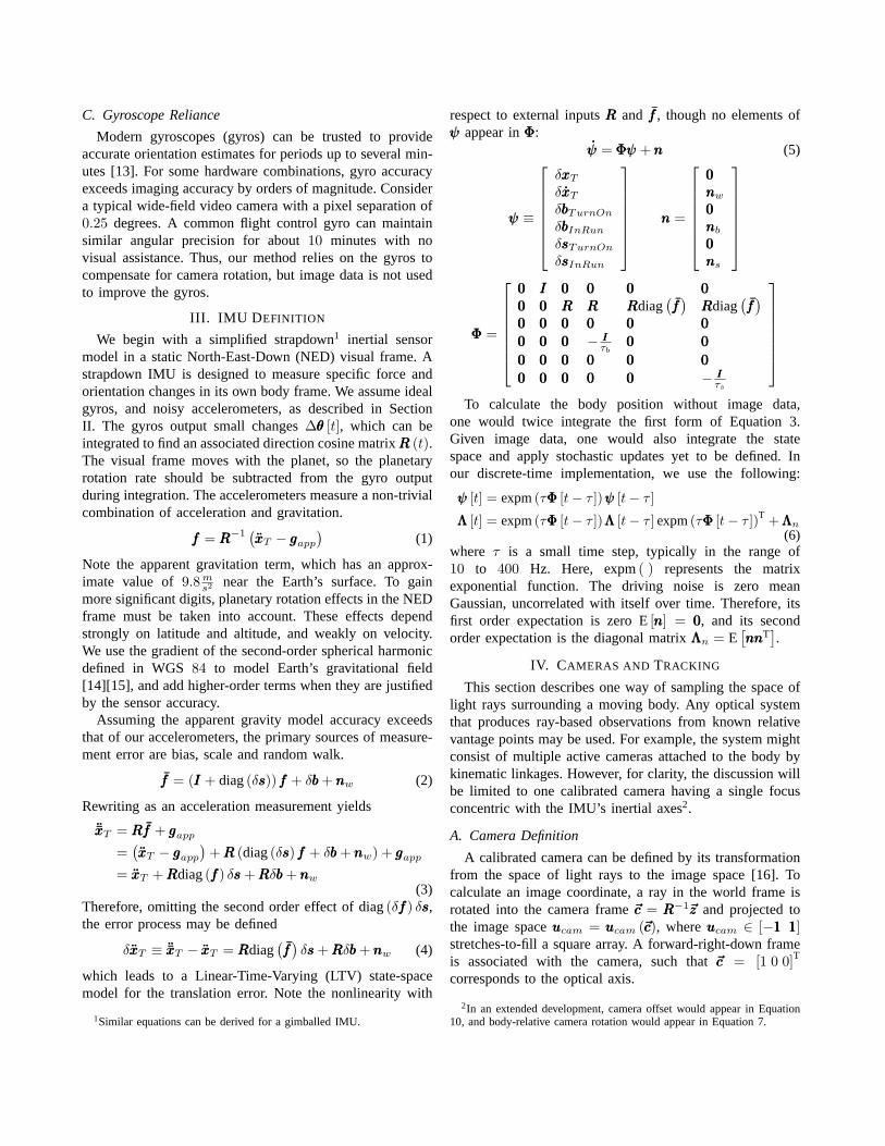
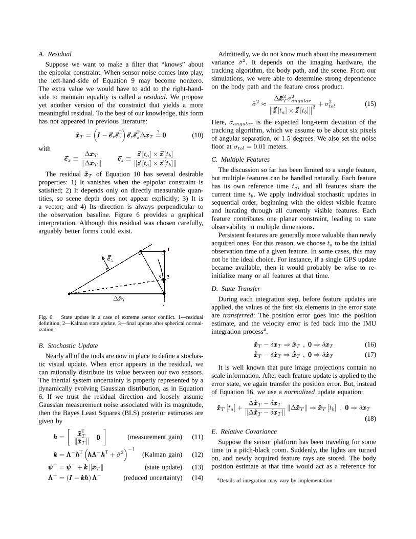
Fig. 4. Demonstration of rotation compensation, corner detection, andtracking applied to the Factory7 scene. Features are boxed and colored fordiagnostic purposes.
V. EPIPOLAR CONSTRAINT FILTER
Consider a single feature tracked over multiple frames.Any two camera poses and a jointly observed feature definea plane, as shown in Figure 5. This well known relationshipis often called theepipolar constraint[12][20][21], thoughit appears in various forms and under different names. Usingour notation, a basic form is given by
(~z~z~z [ta]× ~z~z~z [tb]) ◦∆xxxT = 0 (9)
where∆ represents a change between two timesta andtb.
Fig. 5. The epipolar constraint, satisfied by ideal sensor data.
A. Residual
Suppose we want to make a filter that “knows” aboutthe epipolar constraint. When sensor noise comes into play,the left-hand-side of Equation 9 may become nonzero.The extra value we would have to add to the right-hand-side to maintain equality is called aresidual. We proposeyet another version of the constraint that yields a moremeaningful residual. To the best of our knowledge, this formhas not appeared in previous literature:
xxxT =(III −~e~e~ex~e~e~e
Tx
)~e~e~ez~e~e~e
Tz∆xxxT
?= 000 (10)
with
~e~e~ex ≡∆xxxT
‖∆xxxT ‖~e~e~ez ≡
~z~z~z [ta]× ~z~z~z [tb]‖~z~z~z [ta]× ~z~z~z [tb]‖
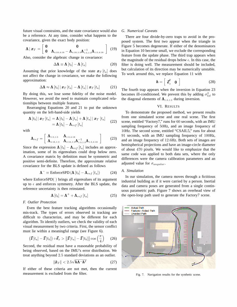
The residualxxxT of Equation 10 has several desirableproperties: 1) It vanishes when the epipolar constraint issatisfied; 2) It depends only on directly measurable quan-tities, so scene depth does not appear explicitly; 3) It isa vector; and 4) Its direction is always perpendicular tothe observation baseline. Figure 6 provides a graphicalinterpretation. Although this residual was chosen carefully,arguably better forms could exist.
Fig. 6. State update in a case of extreme sensor conflict. 1—residualdefinition, 2—Kalman state update, 3—final update after spherical normal-ization.
B. Stochastic Update
Nearly all of the tools are now in place to define a stochas-tic visual update. When error appears in the residual, wecan rationally distribute its value between our two sensors.The inertial system uncertainty is properly represented by adynamically evolving Gaussian distribution, as in Equation6. If we trust the residual direction and loosely assumeGaussian measurement noise associated with its magnitude,then the Bayes Least Squares (BLS) posterior estimates aregiven by
hhh =[
xxxTT
‖xxxT ‖000
](measurement gain) (11)
kkk = ΛΛΛ−hhhT(hΛhΛhΛ−hhhT + σ2
)−1
(Kalman gain) (12)
ψψψ+ = ψψψ− + kkk ‖xxxT ‖ (state update) (13)
ΛΛΛ+ = (III − khkhkh)ΛΛΛ− (reduced uncertainty) (14)
Admittedly, we do not know much about the measurementvariance σ2. It depends on the imaging hardware, thetracking algorithm, the body path, and the scene. From oursimulations, we were able to determine strong dependenceon the body path and the feature cross product.
σ2 ≈∆xxx2
Tσ2angular∥∥~z~z~z [ta]× ~z~z~z [tb]
∥∥2 + σ2tol (15)
Here, σangular is the expected long-term deviation of thetracking algorithm, which we assume to be about six pixelsof angular separation, or1.5 degrees. We also set the noisefloor at σtol = 0.01 meters.
C. Multiple Features
The discussion so far has been limited to a single feature,but multiple features can be handled naturally. Each featurehas its own reference timeta, and all features share thecurrent timetb. We apply individual stochastic updates insequential order, beginning with the oldest visible featureand iterating through all currently visible features. Eachfeature contributes one planar constraint, leading to stateobservability in multiple dimensions.
Persistent features are generally more valuable than newlyacquired ones. For this reason, we chooseta to be the initialobservation time of a given feature. In some cases, this maynot be the ideal choice. For instance, if a single GPS updatebecame available, then it would probably be wise to re-initialize many or all features at that time.
D. State Transfer
During each integration step, before feature updates areapplied, the values of the first six elements in the error stateare transferred: The position error goes into the positionestimate, and the velocity error is fed back into the IMUintegration process4.
xxxT − δxxxT ⇒ xxxT , 000 ⇒ δxxxT (16)˙xxxT − δxxxT ⇒ ˙xxxT , 000 ⇒ δxxxT (17)
It is well known that pure image projections contain noscale information. After each feature update is applied to theerror state, we again transfer the position error. But, insteadof Equation 16, we use anormalizedupdate equation:
xxxT [ta] +∆xxxT − δxxxT
‖∆xxxT − δxxxT ‖‖∆xxxT ‖ ⇒ xxxT [tb] , 000 ⇒ δxxxT
(18)
E. Relative Covariance
Suppose the sensor platform has been traveling for sometime in a pitch-black room. Suddenly, the lights are turnedon, and newly acquired feature rays are stored. The bodyposition estimate at that time would act as a reference for
4Details of integration may vary by implementation.
future visual constraints, and the state covariance would alsobe a reference. At any time, consider what happens to thecovariance, given the exact body position:
ΛΛΛ | xxxT =[
000 000000 ΛΛΛ4:18,4:18 −ΛΛΛ4:18,1:3ΛΛΛ
−11:3,1:3ΛΛΛ1:3,4:18
](19)
Also, consider the algebraic change in covariance:
∆ΛΛΛ ≡ ΛΛΛ [tb]−ΛΛΛ [ta] (20)
Assuming that prior knowledge of the statexxxT [ta] doesnot affect the change in covariance, we make the followingapproximation:
∆ΛΛΛ ≈ ΛΛΛ [tb] | xxxT [ta] −ΛΛΛ [ta] | xxxT [ta] (21)
By doing this, we lose some fidelity of the noise model.However, we avoid the need to maintain complicated rela-tionships between multiple features.
Rearranging Equations 20 and 21 to put the unknownquantity on the left-hand-side yields
ΛΛΛ [tb] | xxxT [ta] = ΛΛΛ [tb]−ΛΛΛ [ta] + ΛΛΛ [ta] | xxxT [ta]= ΛΛΛ [tb]−ΛΛΛref [ta]
(22)
with
ΛΛΛref =[
ΛΛΛ1:3,1:3 ΛΛΛ1:3,4:18
ΛΛΛ4:18,1:3 ΛΛΛ4:18,1:3ΛΛΛ−11:3,1:3ΛΛΛ1:3,4:18
](23)
Since the expressionΛΛΛ [tb] −ΛΛΛref [ta] includes an approx-imation, some of its eigenvalues could drop below zero.A covariance matrix by definition must be symmetric andpositive semi-definite. Therefore, the approximate relativecovariance for the BLS update is defined as follows
ΛΛΛ− ≡ EnforceSPD(ΛΛΛ [tb]−ΛΛΛref [ta]) (24)
where EnforceSPD( ) brings all eigenvalues of its argumentup to ε and enforces symmetry. After the BLS update, thereference uncertainty is then reinstated.
ΛΛΛ [tb] = ΛΛΛ+ + ΛΛΛref [ta] (25)
F. Outlier Protection
Even the best feature tracking algorithms occasionallymis-track. The types of errors observed in tracking aredifficult to characterize, and may be different for eachalgorithm. To identify outliers, we check the validity of eachvisual measurement by two criteria. First, the sensor conflictmust lie within a meaningful range (see Figure 6).(
~z~z~z [ta]− ~z~z~z [tb])◦ ~e~e~ex >
∥∥~z~z~z [ta]− ~z~z~z [tb]∥∥ cos
(π4
)(26)
Second, the residual must have a reasonable probability ofbeing observed, based on the IMU’s error distribution. Wetreat anything beyond2.5 standard deviations as an outlier.
‖xxxT ‖ < 2.5√hΛhΛhΛ−hhhT (27)
If either of these criteria are not met, then the currentmeasurement is excluded from the filter.
G. Numerical Caveats
There are four divide-by-zero traps to avoid in the pro-posed system. The first two appear when the triangle inFigure 5 becomes degenerate. If either of the denominatorsin Equation 10 become small, we exclude the correspondingfeature from the update phase. The third trap appears whenthe magnitude of the residual drops belowε. In this case, thefilter is doing well. The measurement should be included,but calculation of its direction may be numerically unstable.To work around this, we replace Equation 11 with
hhh =[~e~e~e
Tz 000
](28)
The fourth trap appears when the inversion in Equation 23becomes ill-conditioned. We prevent this by addingσ2
tol tothe diagonal elements ofΛΛΛ1:3,1:3 during inversion.
VI. RESULTS
To demonstrate the proposed method, we present resultsfrom one simulated scene and one real scene. The firstscene, entitled “Factory7,” runs for60 seconds, with an IMUsampling frequency of50Hz, and an image frequency of10Hz. The second scene, entitled “CSAIL5,” runs for about91 seconds, with an IMU sampling frequency of100Hz,and an image frequency of12.6Hz. Both sets of images arehemispherical projections and have an image-circle diameterof about470 pixels. We would like to emphasize that thesame code was applied to both data sets, where the onlydifferences were the camera calibration parameters and anadjusted value forσangular.
A. Simulation
In our simulation, the camera moves through a fictitiousindustrial building as if it were carried by a person. Inertialdata and camera poses are generated from a single contin-uous parametric path. Figure 7 shows an overhead view ofthe open-loop path used to generate the Factory7 scene.
Fig. 7. Navigation results for the synthetic scene.
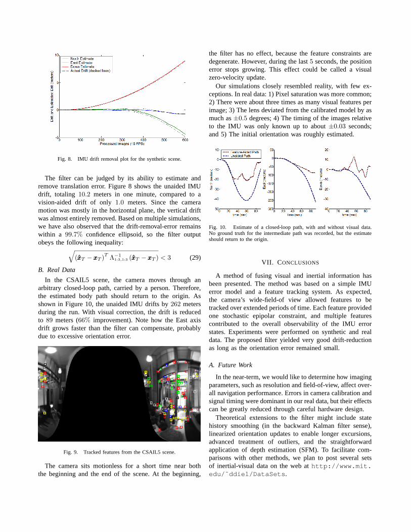
Fig. 8. IMU drift removal plot for the synthetic scene.
The filter can be judged by its ability to estimate andremove translation error. Figure 8 shows the unaided IMUdrift, totaling 10.2 meters in one minute, compared to avision-aided drift of only 1.0 meters. Since the cameramotion was mostly in the horizontal plane, the vertical driftwas almost entirely removed. Based on multiple simulations,we have also observed that the drift-removal-error remainswithin a 99.7% confidence ellipsoid, so the filter outputobeys the following inequality:√
(xxxT − xxxT )T Λ−11:3,1:3 (xxxT − xxxT ) < 3 (29)
B. Real Data
In the CSAIL5 scene, the camera moves through anarbitrary closed-loop path, carried by a person. Therefore,the estimated body path should return to the origin. Asshown in Figure 10, the unaided IMU drifts by262 metersduring the run. With visual correction, the drift is reducedto 89 meters (66% improvement). Note how the East axisdrift grows faster than the filter can compensate, probablydue to excessive orientation error.
Fig. 9. Tracked features from the CSAIL5 scene.
The camera sits motionless for a short time near boththe beginning and the end of the scene. At the beginning,
the filter has no effect, because the feature constraints aredegenerate. However, during the last5 seconds, the positionerror stops growing. This effect could be called a visualzero-velocity update.
Our simulations closely resembled reality, with few ex-ceptions. In real data: 1) Pixel saturation was more common;2) There were about three times as many visual features perimage; 3) The lens deviated from the calibrated model by asmuch as±0.5 degrees; 4) The timing of the images relativeto the IMU was only known up to about±0.03 seconds;and 5) The initial orientation was roughly estimated.
Fig. 10. Estimate of a closed-loop path, with and without visual data.No ground truth for the intermediate path was recorded, but the estimateshould return to the origin.
VII. C ONCLUSIONS
A method of fusing visual and inertial information hasbeen presented. The method was based on a simple IMUerror model and a feature tracking system. As expected,the camera’s wide-field-of view allowed features to betracked over extended periods of time. Each feature providedone stochastic epipolar constraint, and multiple featurescontributed to the overall observability of the IMU errorstates. Experiments were performed on synthetic and realdata. The proposed filter yielded very good drift-reductionas long as the orientation error remained small.
A. Future Work
In the near-term, we would like to determine how imagingparameters, such as resolution and field-of-view, affect over-all navigation performance. Errors in camera calibration andsignal timing were dominant in our real data, but their effectscan be greatly reduced through careful hardware design.
Theoretical extensions to the filter might include statehistory smoothing (in the backward Kalman filter sense),linearized orientation updates to enable longer excursions,advanced treatment of outliers, and the straightforwardapplication of depth estimation (SFM). To facilitate com-parisons with other methods, we plan to post several setsof inertial-visual data on the web athttp://www.mit.edu/˜ddiel/DataSets .
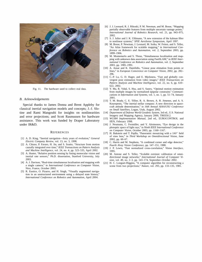
Fig. 11. The hardware used to collect real data.
B. Acknowledgements
Special thanks to James Donna and Brent Appleby forclassical inertial navigation models and concepts; J.-J. Slo-tine and Rami Mangoubi for insights on nonlinearitiesand error projections; and Scott Rasmussen for hardwareassistance. This work was funded by Draper Laboratoryunder IR&D.
REFERENCES
[1] A. D. King, “Inertial navigation—forty years of evolution,”GeneralElectric Company Review, vol. 13, no. 3, 1998.
[2] A. Chiuso, P. Favaro, H. Jin, and S. Soatto, “Structure from motioncausally integrated over time,”IEEE Transactions on Pattern Analysisand Machine Intelligence, vol. 24, no. 4, pp. 523–535, April 2002.
[3] A. Huster, “Relative position sensing by fusing monocular vision andinertial rate sensors,” Ph.D. dissertation, Stanford University, July2003.
[4] A. J. Davison, “Real-time simultaneous localisation and mapping witha single camera,” inInternational Conference on Computer Vision,Nice, France, October 2003.
[5] R. Eustice, O. Pizarro, and H. Singh, “Visually augmented naviga-tion in an unstructured environment using a delayed state history,”International Conference on Robotics and Automation, April 2004.
[6] J. J. Leonard, R. J. Rikoski, P. M. Newman, and M. Bosse, “Mappingpartially observable features from multiple uncertain vantage points,”International Journal of Robotics Research, vol. 21, pp. 943–975,2002.
[7] S. J. Julier and J. K. Uhlmann, “A new extension of the kalman filterto nonlinear systems,”SPIE AeroSense Symposium, April 1997.
[8] M. Bosse, P. Newman, J. Leonard, M. Soika, W. Feiten, and S. Teller,“An Atlas framework for scalable mapping,” inInternational Con-ference on Robotics and Automation, vol. 2, September 2003, pp.1899–1906.
[9] M. Montemerlo and S. Thrun, “Simultaneous localization and map-ping with unknown data association using FastSLAM,” inIEEE Inter-national Conference on Robotics and Automation, vol. 2, September2003, pp. 1985–1991.
[10] A. Ansar and K. Daniilidis, “Linear pose etimation from points orlines,” in European Converence on Computer Vision, 2002, pp. 282–296.
[11] C.-P. Lu, G. D. Hager, and E. Mjolsness, “Fast and globally con-vergent pose estimation from video images,”IEEE Transactions onPattern Analysis and Machine Intelligence, vol. 22, no. 6, pp. 610–622, 2002.
[12] Y. Ma, R. Vidal, S. Hsu, and S. Sastry, “Optimal motion estimationfrom multiple images by normalized epipolar constraint,”Communi-cations in Information and Systems, vol. 1, no. 1, pp. 51–74, January2001.
[13] T. M. Brady, C. E. Tillier, R. A. Brown, A. R. Jimenez, and A. S.Kourepenis, “The inertial stellar compass: A new direction in space-craft attitude determination,” in16th Annual AIAA/USU Conferenceon Small Satellites, Logan, Utah, August 2002.
[14] Department of Defense World Geodetic System, 3rd ed., U.S. NationalImagery and Mapping Agency, January 2000, TR8350.2.
[15] WGS84 Implementation Manual, 2nd ed., EUROCONTROL andIfEN, February 1998.
[16] J. Neumann, C. Fermuller, and Y. Aloimonos, “Eye design in theplenoptic space of light rays,” inNinth IEEE International Conferenceon Computer Vision, October 2003, pp. 1160–1167.
[17] H. Bakstein and T. Pajdla, “Panoramic mosaicing with a180◦ fieldof view lens,” in Third Workshop on Omnidirectional Vision, June2002, pp. 60–67.
[18] C. Harris and M. Stephens, “A combined corner and edge detector,”Fourth Alvey Vision Conference, pp. 147–151, 1988.
[19] J. P. Lewis, “Fast normalized cross-correlation,”Vision Interface,1995.
[20] M. Antone and S. Teller, “Scalable extrinsic calibration of omni-directional image networks,”International Journal of Computer Vi-sion, vol. 49, no. 2–3, pp. 143–174, September–October 2002.
[21] H. C. Longuet-Higgins, “A computer algorithm for reconstructing ascene from two projections,”Nature, vol. 293, pp. 133–135, 1981.