EPSII

59:006

Spring 2004

Topics Using TextPad If Statements Relational Operators Nested If Statements Else and Elseif Clauses Logical Functions For Loops While Loops User Functions

TextPad

TextPad is a Convenient Tool in the CSS Windows Environment for Writing Code

It Recognizes Syntax Error Automatically Can Save Files Corrected for the Unix

Environment for Importing Check it out! (I know, it’s a little late)

Back to Matlab

If Statements

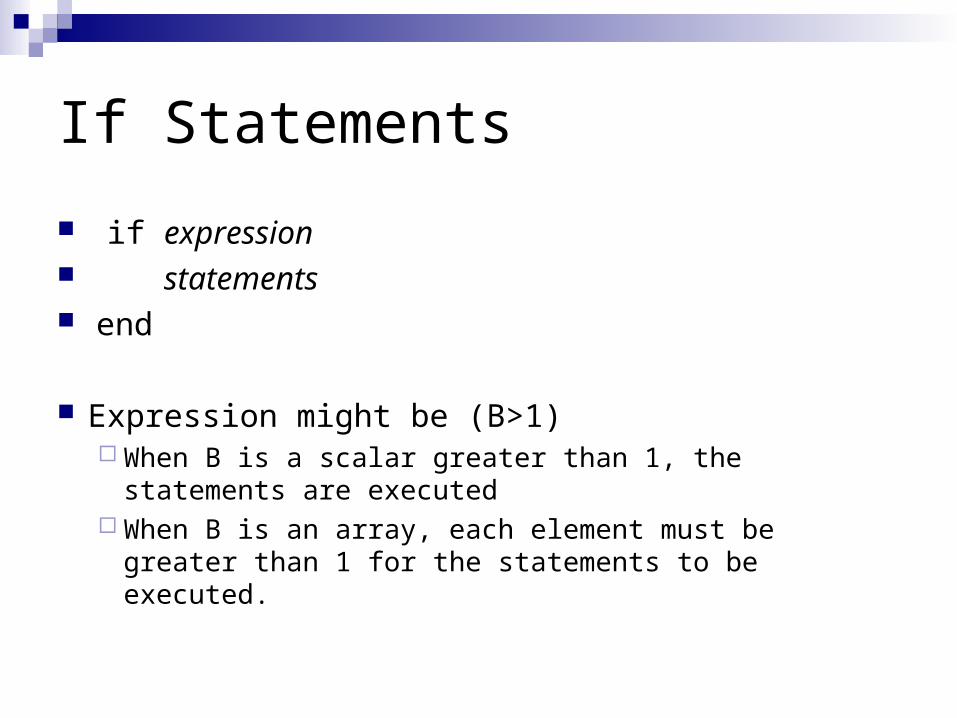
if expression statements end

Expression might be (B>1) When B is a scalar greater than 1, the statements are

executed When B is an array, each element must be greater than

1 for the statements to be executed.

Relational Operators

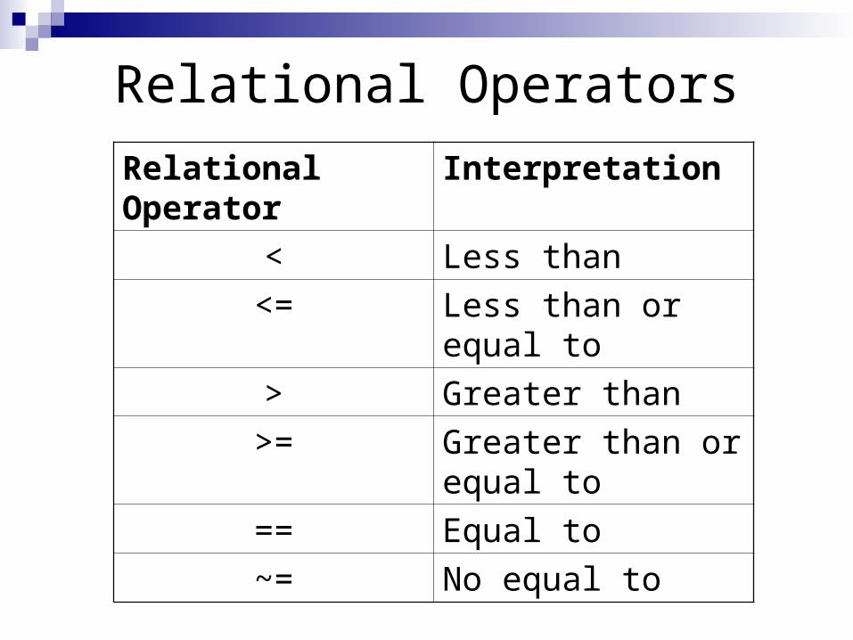
Relational Operator

Interpretation

< Less than

<= Less than or equal to

> Greater than

>= Greater than or equal to

== Equal to

~= No equal to

Using Relational Operators

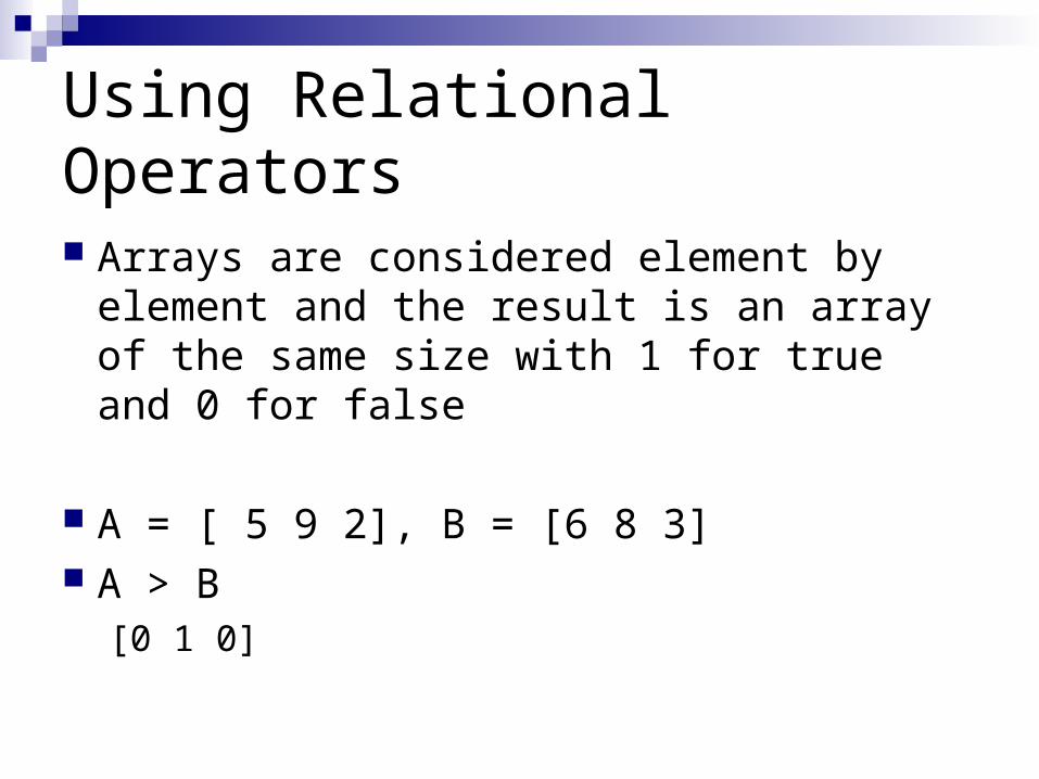
Arrays are considered element by element and the result is an array of the same size with 1 for true and 0 for false

A = [ 5 9 2], B = [6 8 3] A > B

[0 1 0]

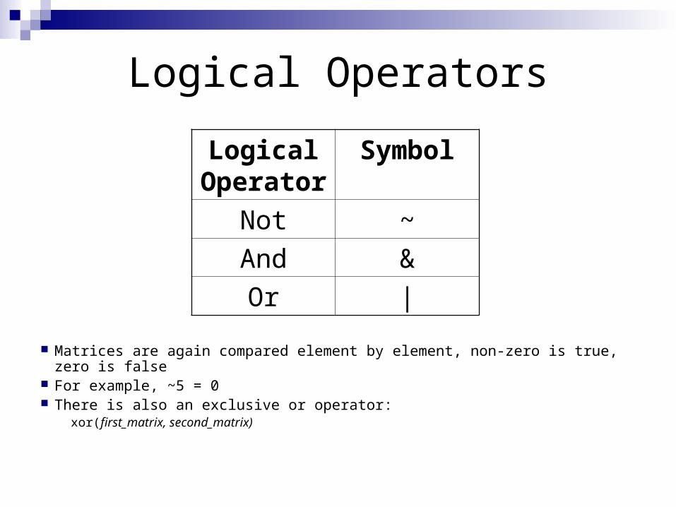
Logical Operators

Matrices are again compared element by element, non-zero is true, zero is false For example, ~5 = 0 There is also an exclusive or operator:

xor(first_matrix, second_matrix)

Logical Operator

Symbol

Not ~

And &

Or |

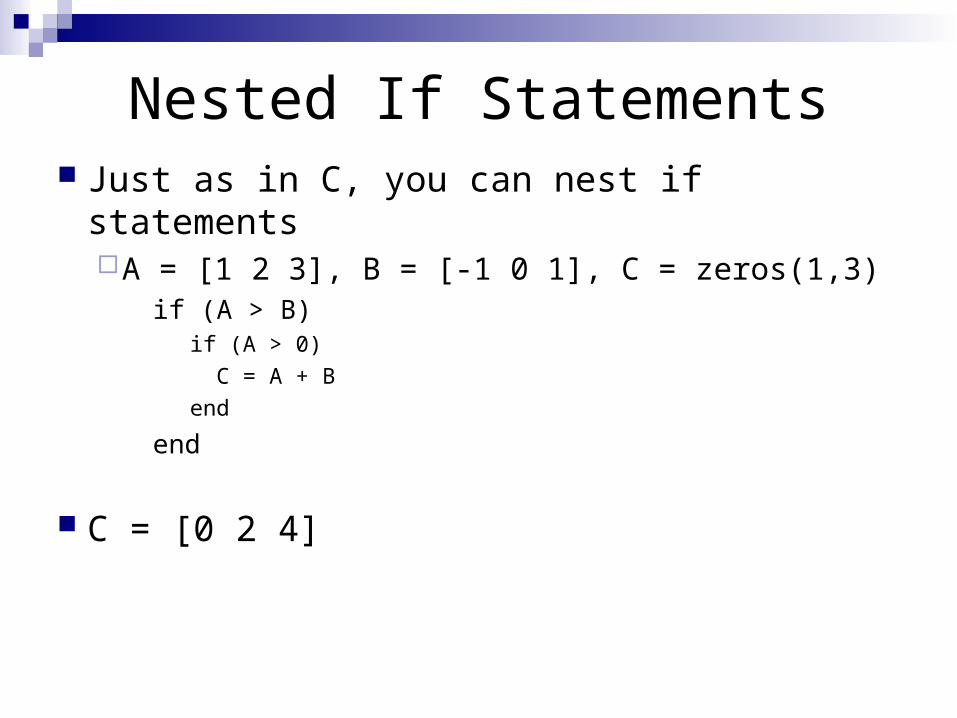
Nested If Statements Just as in C, you can nest if statements

A = [1 2 3], B = [-1 0 1], C = zeros(1,3) if (A > B)

if (A > 0)

C = A + B

end

end

C = [0 2 4]

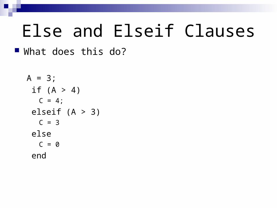
Else and Elseif Clauses What does this do?

A = 3;

if (A > 4)C = 4;

elseif (A > 3)C = 3

elseC = 0

end

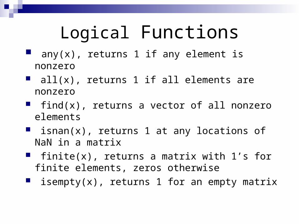
Logical Functions any(x), returns 1 if any element is nonzero all(x), returns 1 if all elements are nonzero find(x), returns a vector of all nonzero

elements isnan(x), returns 1 at any locations of NaN in a

matrix finite(x), returns a matrix with 1’s for finite

elements, zeros otherwise isempty(x), returns 1 for an empty matrix

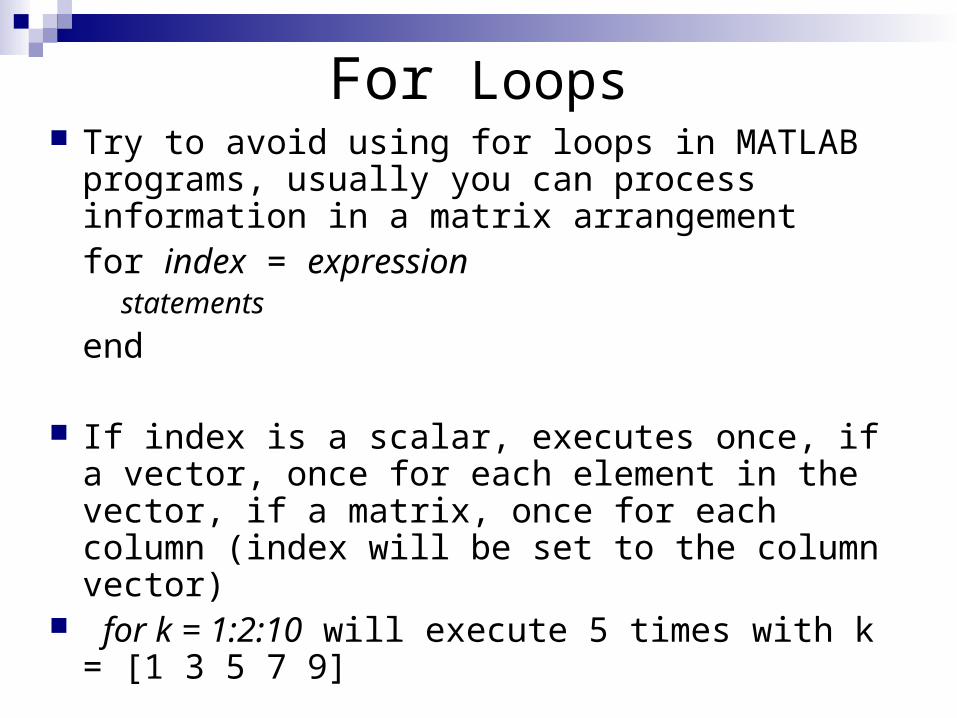
For Loops Try to avoid using for loops in MATLAB

programs, usually you can process information in a matrix arrangement

for index = expressionstatements

end

If index is a scalar, executes once, if a vector, once for each element in the vector, if a matrix, once for each column (index will be set to the column vector)

for k = 1:2:10 will execute 5 times with k = [1 3 5 7 9]

While loops

while expression statements

end

Executes as long as the expression is true

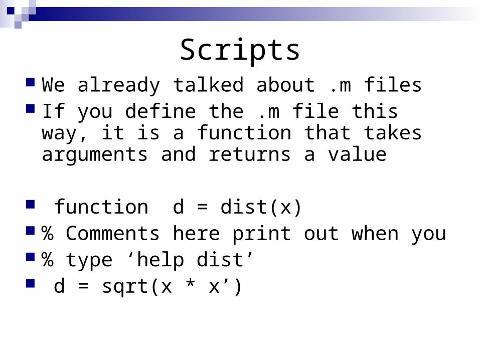
Scripts We already talked about .m files If you define the .m file this way, it is a

function that takes arguments and returns a value

function d = dist(x) % Comments here print out when you % type ‘help dist’ d = sqrt(x * x’)

Revisit our two tank example

Considering two tank example again. If the tanks are initially at steady state and a step change in from 0.05 to 0.06 at t=200 seconds is introduced, how do the tank levels change with time. Plot the tanks level vs. time for both systems. What is the new steady state value?

q1

h1

q2

h2

1(h1-h2)

2 h21/2

Example Problem

The liquid levels in tank1 and tank 2 are given by

Adh

dtq h h1

11 1 1 2 = ( )

Adh

dtq a h h a h2

22 1 1 2 2 2 = ( )

21

22

1

2

31 2

= cross section area of the tank 1, m

A = cross section area of tank 2, m

h = liquid level in tank 1, m

h = liquid level in tank 2, m

q ,q = flow rates, m /

A

s

T=200 q1 increases

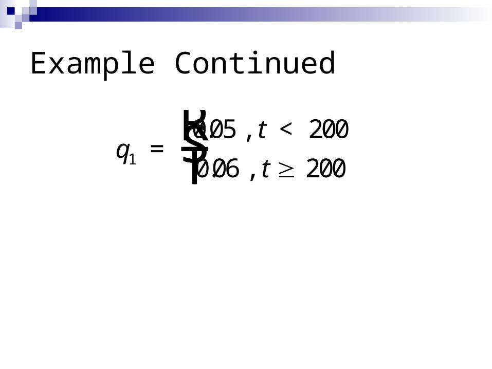
Example Continued

qt

t1

0 05 200

0 06 200 =

. , <

. , RST

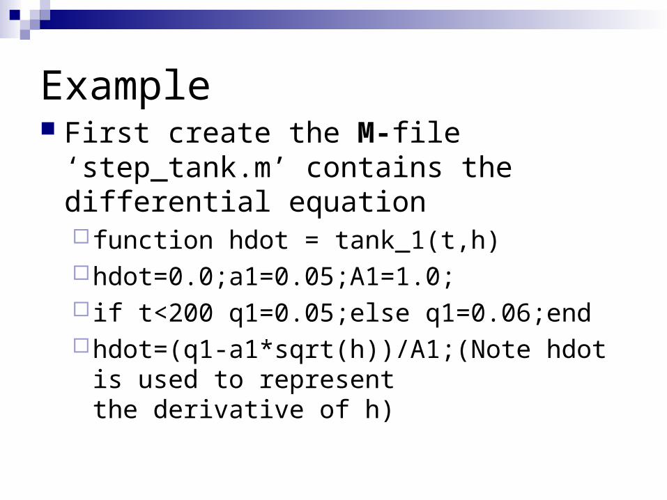
Example First create the M-file ‘step_tank.m’

contains the differential equation function hdot = tank_1(t,h)hdot=0.0;a1=0.05;A1=1.0; if t<200 q1=0.05;else q1=0.06;endhdot=(q1-a1*sqrt(h))/A1;(Note hdot is used to

represent the derivative of h)

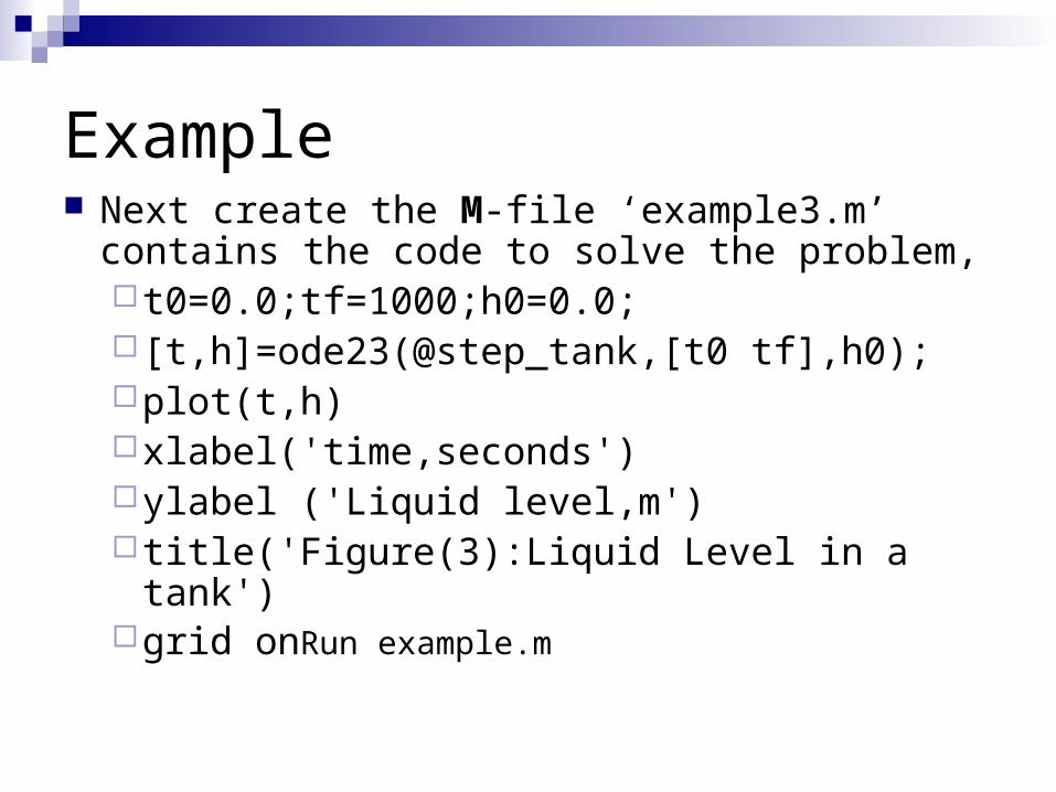
Example Next create the M-file ‘example3.m’ contains the

code to solve the problem, t0=0.0;tf=1000;h0=0.0; [t,h]=ode23(@step_tank,[t0 tf],h0);plot(t,h)xlabel('time,seconds')ylabel ('Liquid level,m') title('Figure(3):Liquid Level in a tank')grid onRun example.m

Introduction to Simulink

The other method MATLAB uses to numerical differentiate (integrate) is via SIMULINK. SIMULINK is a program for simulating dynamic systems. It has two phases of use: model definition and model analysis. Thus you need to first define your model and then use modeling analysis to understand the system’s dynamic behavior.

Introduction to Simulink

SIMULINK has a new class of windows called block diagram windows. After a model is defined, it can be analyzed either using the SIMULINK menus or using MATLAB's command window (workspace).

Introduction to Simulink

Defining the model is easiest if one visualizes the loop for calculating the output as an approximate integration solution for small time steps.

Use drag and drop to connect ‘blocks’ that represent, constants, integrals, operations, inputs and outputs. Easy to connect with lines.

Introduction to Simulink Starting SIMULINK At the MATLAB prompt type simulink or click the simulink button

on the tool bar to open the main block library. From the SIMULINK window select New from the File menu. This

will open an empty window where you can construct your model. Open one or more libraries, and drag the appropriate blocks

(model the above diagram) into the active window. Connect the blocks by drawing lines between then using the

mouse. Open the blocks (by double-clicking) and change their internal

parameters. Block parameters can be any legal MATLAB expression.

Save and re-name the system by choosing Save As from the File menu.

Introduction to Simulink Run a simulation by selecting Start from the Simulation

menu. While a simulation is running the Start item becomes Stop.

Adjust the simulation parameters by selecting Parameters from the Simulation menu.

You can monitor the behavior of the system with scope block or you can use to work place block to send data to the MATLAB workspace and perform MATLAB functions on the results.

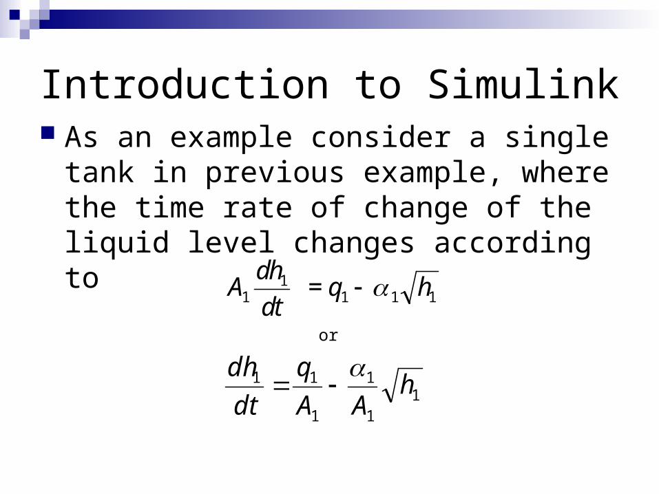
Introduction to Simulink As an example consider a single tank in

previous example, where the time rate of change of the liquid level changes according to

Adh

dtq h1

11 1 1 =

11

1

1

11 hAA

q

dt

dh

or

Introduction to Simulink

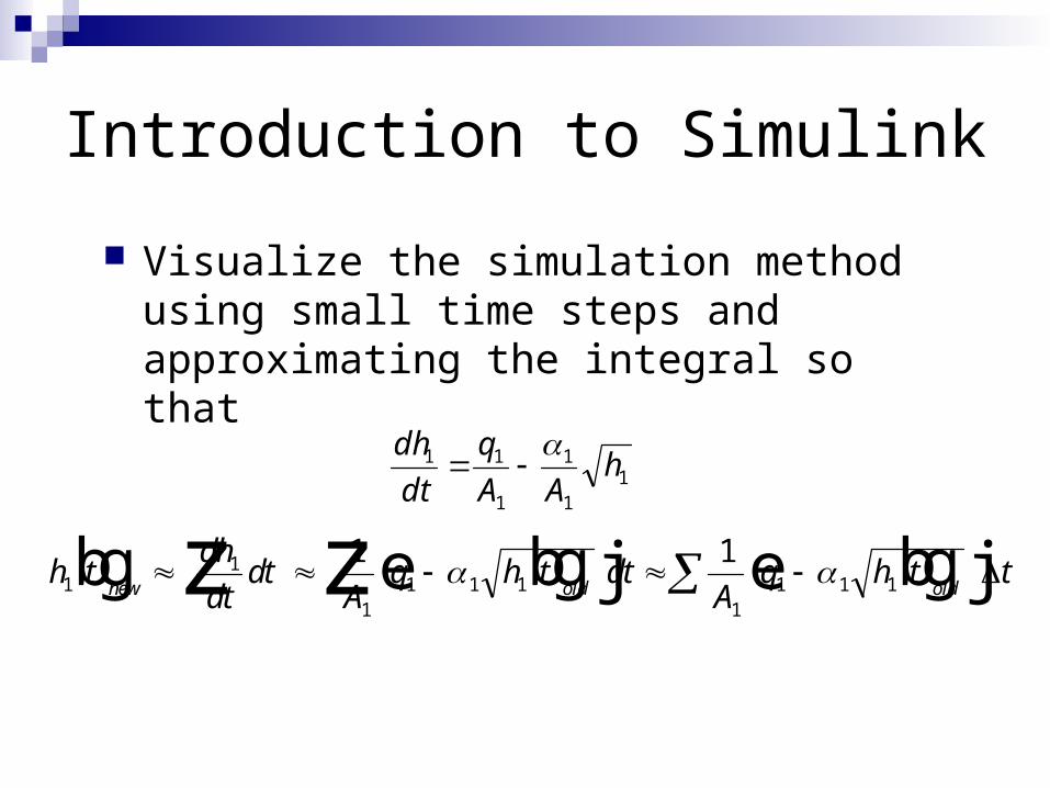
Visualize the simulation method using small time steps and approximating the integral so that

h tdh

dtdt

Aq h t dt

Aq h t t

new old old11

11 1 1

11 1 1

1 1bg bge j bge j z z

11

1

1

11 hAA

q

dt

dh

Introduction to Simulink

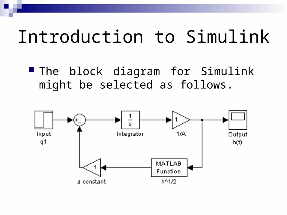
The block diagram for Simulink might be selected as follows.

Introduction to Simulink We obtained this by dragging over the integrator

block, constant blocks, function block, etc. and then connecting them so that they result in the approximate integral shown above. Note that although SIMULINK uses the Laplace transform symbol for integration (1/s), SIMULINK is actually only approximating the solution and, thus, the integrator can be used with non-linear problems (such as this one). (Maybe they think 1/s is more beautiful than the integral sign.)

Introduction to Simulink

The progress of simulation can be viewed while the simulation is running, and the final results can be made available in the MATLAB workspace when a simulation is completed.

Printing in Simulink The best way to obtain a hard copy of the

graph you have generated or to print the block diagram of your model is to use the print provided by MATLAB. It has the following synopsis:

print [-ddevice ] [-options ] [ filename ] Using print alone with no arguments send the

contents of the current figure window to the default printer. While print filename saves the current figure to the designated file.

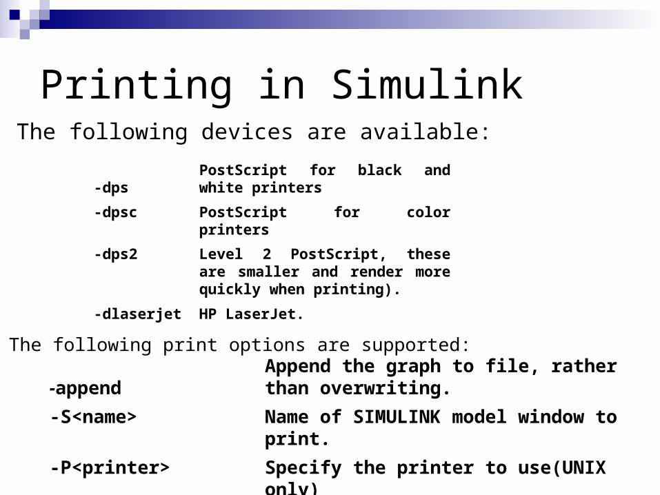
Printing in SimulinkThe following devices are available:

-dpsPostScript for black and white printers

-dpsc PostScript for color printers

-dps2 Level 2 PostScript, these are smaller and render more quickly when printing).

-dlaserjet HP LaserJet.

The following print options are supported:

-appendAppend the graph to file, rather than overwriting.

-S<name> Name of SIMULINK model window to print.

-P<printer> Specify the printer to use(UNIX only)