Embed Size (px)
Citation preview
Energy Systems Research Unit Dept. of Mechanical and Aerospace Engineering Tel: 0141 548 2041; Email: [email protected]
http://www.strath.ac.uk/esru
ESRU Report
EPSRC Research Project EP/G00028X/1
Environmental Assessment of Domestic Laundering
Final Modelling Report
Kelly N J K, Markopoulos A and Strachan P A
March 2012
Environmental Assessment of Domestic Laundering: Modelling Report
Contents
1. Overview of the modelling study and integration with other project modules
2. Modelling capabilities and enhancements
2.1 Integrated moisture flow modelling
2.2 Hygrothermal properties
2.3 Modelling enhancements
2.4 Moisture release modelling
2.5 Parametric test structure
3. Validation
3.1 IEA validation 41 tests
3.2 Cyclic tests
4. Modelling – general parametric study
5. Modelling – specific studies
6. Modelling – realistic case
7. Conclusions
8. References
Note There was a serious fire in early February 2012, towards the end of the project, in the James Weir building at the University of Strathclyde. This interrupted some of the final research and report writing with some computers used in the project not recovered until the end of March. This report has two missing sections: section 3.2, which will describe the comparison of predictions with additional cyclic tests undertaken near the end of the project, and section 6 which will report on a simulation with a detailed realistic user behaviour profile. These sections will be added in the near future with a report update.
Environmental Assessment of Domestic Laundering: Modelling Report
1. Overview of the modelling study and integration with other project modules
The main aim of this EPSRC project was to evaluate the energy consumption and associated
indoor environmental conditions which affect health and comfort as a result of the use of
wet appliances and associated clothes drying, and to suggest practical solutions to problems
identified.
The modelling study was undertaken to quantify the energy and environmental effects of a
range of scenarios associated with laundry, in particular the influence of ventilation,
insulation, moisture buffering and moisture loads. The study had two major inputs from the
other work packages within the project.
Firstly, the housing survey and associated analysis of representative dwellings
undertaken by the Glasgow School of Art enabled typical patterns of wet appliance
use, drying and ironing to be identified. These patterns led to the development of a
number of scenarios that were tested in the modelling work.
Secondly, a barrier to modelling the hygrothermal response of buildings is the
paucity of data on hygrothermal properties of materials. Therefore, an experimental
programme was conducted by Glasgow Caledonian University to obtain the
necessary fundamental material properties for common building internal finishes
and possible moisture control materials. Experiments on moisture release rates for
passive drying of washing loads were also undertaken.
The modelling of heat flow, air flow and moisture flow requires a detailed integrated
modelling approach. The following steps were undertaken to ensure the modelling work
could produce reliable results.
A review of the moisture flow modelling capability in the Open Source simulation
program ESP‐r (2012), which was used for the modelling work in this study, was
undertaken. The thermal and airflow integration capabilities were well established;
integrated moisture flow modelling was less well developed.
Additional capabilities were added to the functionality of the simulation program to
deal with the material hygrothermal properties (vapour permeability and moisture
absorption/desorption) which may have a variety of functions describing the
variation with temperature and humidity.
Moisture release models were added based on the experimental data.
A number of validation exercises were undertaken based on tests published in IEA
Annex 41 (IEA 2005) to ensure model predictions were acceptable.

Environmental Assessment of Domestic Laundering: Modelling Report
These steps are described in Sections 2 and 3 of this report.
The scenario modelling required a large number of parametric variations. This was
undertaken in a systematic way by developing a structured set of scripts. Details are
included in Section 2.
For the scenario modelling, a 3‐step procedure was followed.
The first step was to undertake an initial series of parametric simulations focusing on
lower and upper limits of the main parameters influencing indoor moisture
conditions. The aim of this step was to identify those parameters having the greatest
influence on moisture levels and to establish key areas for further investigation.
The second step involved more specific investigations e.g. comparing ventilation
strategies when moisture control materials are incorporated into the structure.
Lastly, a detailed occupancy and house usage patterns was modelled as an example
of a “realistic” case.
Environmental Assessment of Domestic Laundering: Modelling Report
2. Modelling capabilities and enhancements
2.1 Integrated moisture flow modelling
Heat, air and moisture simulation requires an integrated modelling approach involving the
simultaneous solution of equation‐sets representing the processes occurring in each
technical domain (building‐side heat flow, inter‐space air flow and constructional moisture
flow). Within ESP‐r this is achieved by invoking solvers that are tailored to individual domain
equation‐sets, and placing the solvers under global iteration control to ensure that
appropriate interface variables are exchanged at the required frequency (Clarke 2001).
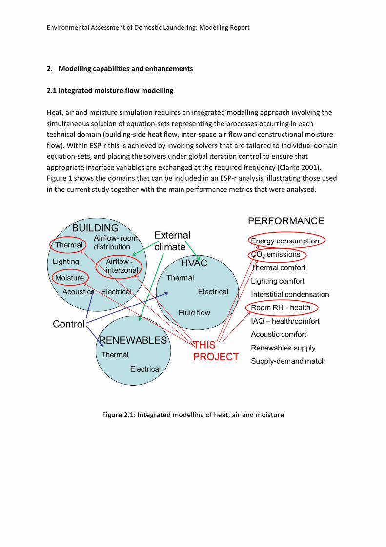
Figure 1 shows the domains that can be included in an ESP‐r analysis, illustrating those used
in the current study together with the main performance metrics that were analysed.
Figure 2.1: Integrated modelling of heat, air and moisture
Environmental Assessment of Domestic Laundering: Modelling Report
A finite volume approach is used for the building thermal analysis (Clarke and Tang 2004)
which includes the conductive, convective, advective and radiative exchanges within the
various thermal zones representing the buidling. The approach is based on a semi‐implicit
scheme, which is second‐order time accurate, unconditionally stable for all space and time
steps and allows time dependent and/or state variable dependent boundary conditions and
coefficients. An optimised numerical technique is employed to solve the system equations
simultaneously, while keeping the required computation to a minimum.
For the inter‐zone air flow, ESP‐r employs a ‘node‐arc’ representation of infiltration and
mechanical ventilation (Clarke and Hensen 1991). A set of non‐linear equations represents
the conservation of mass at nodes as a function of the pressure difference across flow
restrictions (arcs). The flow rates through the flow restrictions are calculated from empirical
relationships that express mass flow as a function of pressure difference. At each timestep
of the simulation, the network is solved based on the known boundary pressure conditions
at that timestep. An iterative solution is required because of the non‐linear flow‐pressure
relationships. The converged solution gives the air flow rates throughout the network
established to represent a building’s infiltration and ventilation, natural and/or mechanical.
The flow of moisture in the air is tracked knowing the moisture concentrations in the
various zones represented by the air flow nodes, together with any specified moisture
source.
Intra‐construction moisture flow was described by Nakhi (1995). Building constructions are
subjected to four wetting phenomena – absorption, vapour transport, capillary
condensation (vapour and liquid transport) and liquid transport – with the driving potentials
for moisture transfer being density gradient (molecular diffusion) and temperature/pressure
gradient (filtration motion).
ESP‐r’s modelling approach is based on mass and energy conservation considerations
applied to homogeneous, isotropic, constructional control volumes and is based on three
principal assumptions: 1) that vapour and liquid flows are slow enough to allow
thermodynamic equilibrium between phases, 2) the filtration flow due to total pressure
difference between inside and outside is negligible and 3) while liquid flow and capillary
condensation is considered in the moisture equations, the associated enthalpies are
combined and estimated from the vapour specific enthalpy alone, with the heat
absorption/dissipation due to phase change assumed to occur at saturation.
For moisture flow the governing mass conservation equation is
Environmental Assessment of Domestic Laundering: Modelling Report
where ρ is density (kg/m3), o and l denote porous media and liquid respectively, ξ is
moisture storage capacity (kg/kg), P is partial water vapour pressure (Pa), Ps is saturated
vapour pressure (Pa), δ is water vapour permeability (kg/Pa.m.s), D is thermal diffusion
coefficient (kg/m2.K.s) and s is a moisture source term (kg/m3.s). X and Y denote
temperature and pressure driving potentials respectively, with the principal potential given
as the subscript.
For energy, the governing equation is
(equation 2.1)
where c is specific heat (J/kg.K), u is moisture content (kg/kg), T is temperature (K), λ is heat
conductivity (W/m.K), Jv is vapour mass flux (kg/m2.s), g is a source of heat (W/m3) and hv, hl
and hs are enthalpies of vapour, liquid and moisture flux sources respectively (J/kg).
For condensation and evaporation processes, a control equation is implemented as a one‐
way liquid valve connected to the control volume. When the relative humidity reaches its
maximum value, the valve opens to deliver the condensate to an imaginary tank.
Conversely, when the relative humidity falls below its maximum value, liquid is returned to
the control volume where it re‐evaporates. At the present time this process is implemented
as a function of the saturation pressure only with no account of capillary condensation.
Application of these coupled equations allows for the solution of the three dependent
variables, P, T and ρl, for each control volume within a construction when evolving under the
influence of boundary heat and mass transfers being simultaneously resolved within the
connected domain models as described above. To achieve this solution, a finite difference
approximation is applied to the foregoing equations.
For moisture:
Environmental Assessment of Domestic Laundering: Modelling Report
∆
1 ∆
(equation 2.2)
where γ is the degree of implicitness, n and n+1 refer to the present and future time‐rows of
some arbitrary simulation time step, Δt (s), m the specific mass (kg/m3), and
→∆
∆ →
1 →∆
∆ →
→∆
∆ →
1 →∆
∆ →
(equation 2.3)
where A is area (m2), ΔX is flow‐path length (m) and V is volume (m3).
For energy:
Environmental Assessment of Domestic Laundering: Modelling Report
∆ ∆
1 ∆ 1 ∆
(equation 2.4)
where
→∆
∆ →
1 →∆
∆ →
.
The moisture storage capacity, ξ, in equation 2.3 is found from an expression by Hansen
(1986):
1.0 ; 0 1
(equation 2.5)
where φ is relative humidity and a mass‐weighted value of ξ is used where the control
volume material is heterogeneous. The calculation of the vapour permeability δ is described
in section 2.2.
The coupled moisture/energy equations for a given system are then given by
where E and M are the energy and moisture coefficient matrices respectively, T and P are
the temperature and vapour pressure vectors, and Be and Bm are the energy and moisture
boundary conditions.
Environmental Assessment of Domestic Laundering: Modelling Report
With temperature and partial vapour pressure used as the transport potentials for moisture,
the model gives rise to a coupled heat and moisture transport model.
2.2 Hygrothermal Properties
In order to model the behaviour of moisture in hygroscopic material, ESP‐r requires the implementation of specific hygrothermal property data. This data is provided in the form of moisture diffusion coefficients. These values relate to the vapour permeability and the sorption isotherm function of a particular material in the model construction, necessary for ESP‐r to calculate the rate of moisture transfer. The equations used by ESP‐r to calculate these two material properties are explained below in further detail. 2.2.1 Vapour Permeability:
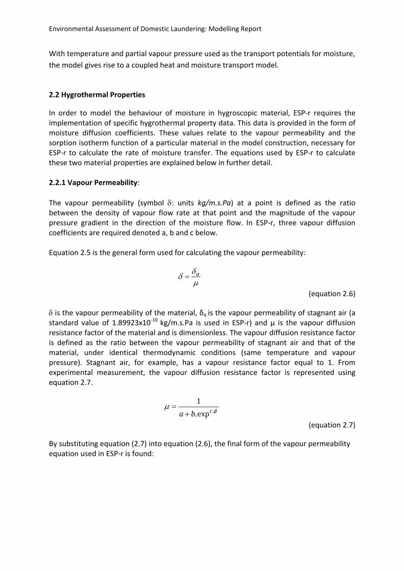
The vapour permeability (symbol : units kg/m.s.Pa) at a point is defined as the ratio between the density of vapour flow rate at that point and the magnitude of the vapour pressure gradient in the direction of the moisture flow. In ESP‐r, three vapour diffusion coefficients are required denoted a, b and c below. Equation 2.5 is the general form used for calculating the vapour permeability:
a
(equation 2.6) is the vapour permeability of the material, δa is the vapour permeability of stagnant air (a standard value of 1.89923x10‐10 kg/m.s.Pa is used in ESP‐r) and µ is the vapour diffusion resistance factor of the material and is dimensionless. The vapour diffusion resistance factor is defined as the ratio between the vapour permeability of stagnant air and that of the material, under identical thermodynamic conditions (same temperature and vapour pressure). Stagnant air, for example, has a vapour resistance factor equal to 1. From experimental measurement, the vapour diffusion resistance factor is represented using equation 2.7.
.exp.
1cba
(equation 2.7)
By substituting equation (2.7) into equation (2.6), the final form of the vapour permeability equation used in ESP‐r is found:
Environmental Assessment of Domestic Laundering: Modelling Report
ca ba exp.
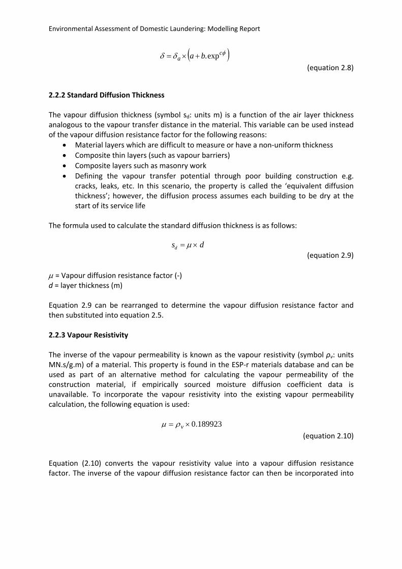
(equation 2.8) 2.2.2 Standard Diffusion Thickness The vapour diffusion thickness (symbol sd: units m) is a function of the air layer thickness analogous to the vapour transfer distance in the material. This variable can be used instead of the vapour diffusion resistance factor for the following reasons:
Material layers which are difficult to measure or have a non‐uniform thickness
Composite thin layers (such as vapour barriers)
Composite layers such as masonry work
Defining the vapour transfer potential through poor building construction e.g. cracks, leaks, etc. In this scenario, the property is called the ‘equivalent diffusion thickness’; however, the diffusion process assumes each building to be dry at the start of its service life
The formula used to calculate the standard diffusion thickness is as follows:
sd d
(equation 2.9)
= Vapour diffusion resistance factor (‐) d = layer thickness (m) Equation 2.9 can be rearranged to determine the vapour diffusion resistance factor and then substituted into equation 2.5. 2.2.3 Vapour Resistivity The inverse of the vapour permeability is known as the vapour resistivity (symbol ρv: units MN.s/g.m) of a material. This property is found in the ESP‐r materials database and can be used as part of an alternative method for calculating the vapour permeability of the construction material, if empirically sourced moisture diffusion coefficient data is unavailable. To incorporate the vapour resistivity into the existing vapour permeability calculation, the following equation is used:
189923.0 v (equation 2.10)
Equation (2.10) converts the vapour resistivity value into a vapour diffusion resistance factor. The inverse of the vapour diffusion resistance factor can then be incorporated into
Environmental Assessment of Domestic Laundering: Modelling Report
equation (2.8) to represent the coefficient labelled ‘a’, so that the vapour permeability can be calculated. 2.2.4 Vapour Permeance The vapour permeance (symboldl:units kg/Pa.m
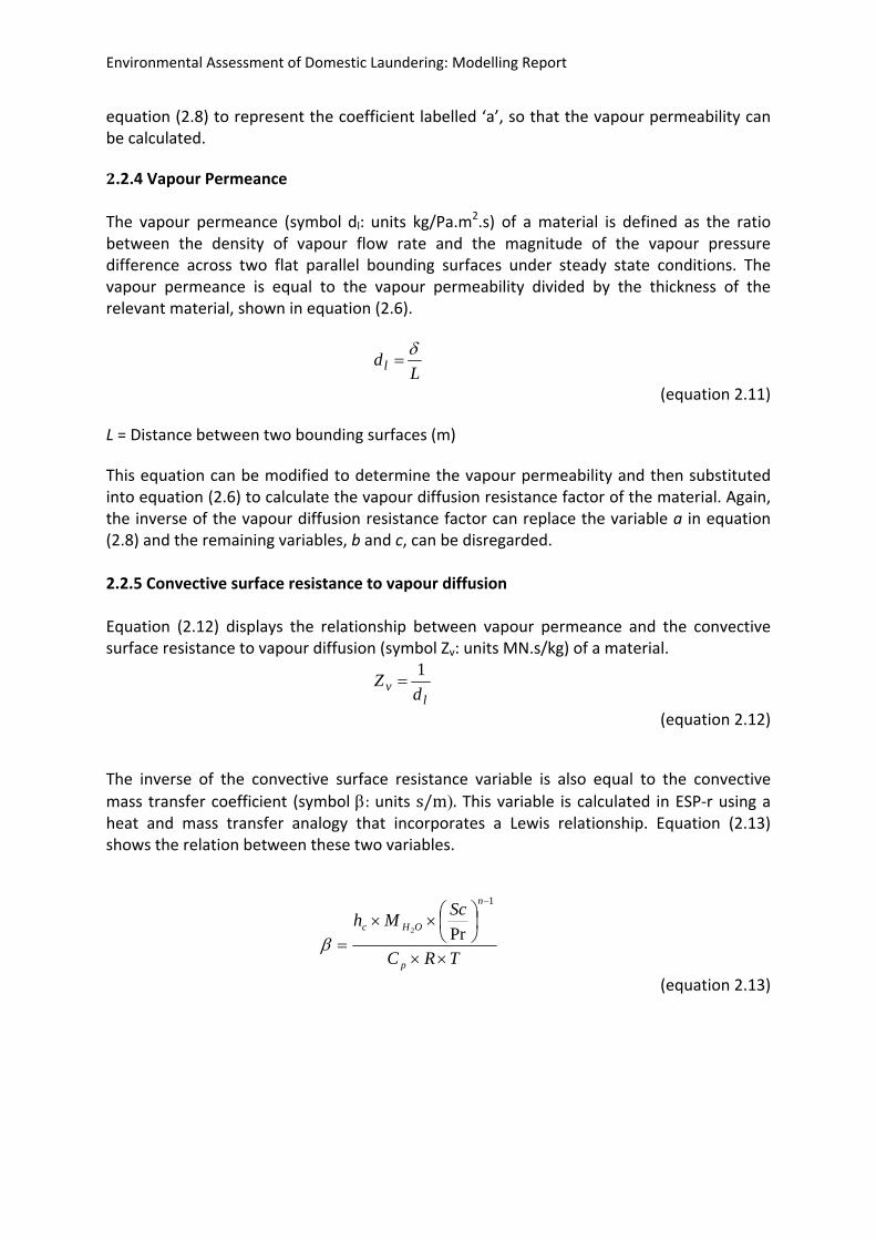
2.s) of a material is defined as the ratio between the density of vapour flow rate and the magnitude of the vapour pressure difference across two flat parallel bounding surfaces under steady state conditions. The vapour permeance is equal to the vapour permeability divided by the thickness of the relevant material, shown in equation (2.6).
Ldl
(equation 2.11)L = Distance between two bounding surfaces (m) This equation can be modified to determine the vapour permeability and then substituted into equation (2.6) to calculate the vapour diffusion resistance factor of the material. Again, the inverse of the vapour diffusion resistance factor can replace the variable a in equation (2.8) and the remaining variables, b and c, can be disregarded. 2.2.5 Convective surface resistance to vapour diffusion Equation (2.12) displays the relationship between vapour permeance and the convective surface resistance to vapour diffusion (symbol Zv: units MN.s/kg) of a material.
l
v dZ
1
(equation 2.12) The inverse of the convective surface resistance variable is also equal to the convective
mass transfer coefficient (symbol:units s/m.This variable is calculated in ESP‐r using a heat and mass transfer analogy that incorporates a Lewis relationship. Equation (2.13) shows the relation between these two variables.
TRC
ScMh
p
n
OHc
1
Pr2
(equation 2.13)
Environmental Assessment of Domestic Laundering: Modelling Report
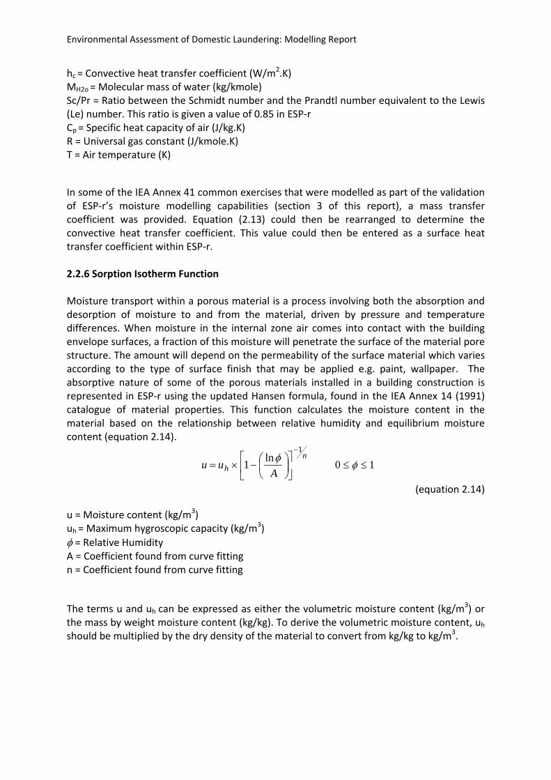
hc = Convective heat transfer coefficient (W/m2.K) MH2o = Molecular mass of water (kg/kmole) Sc/Pr = Ratio between the Schmidt number and the Prandtl number equivalent to the Lewis (Le) number. This ratio is given a value of 0.85 in ESP‐r Cp = Specific heat capacity of air (J/kg.K) R = Universal gas constant (J/kmole.K) T = Air temperature (K)In some of the IEA Annex 41 common exercises that were modelled as part of the validation of ESP‐r’s moisture modelling capabilities (section 3 of this report), a mass transfer coefficient was provided. Equation (2.13) could then be rearranged to determine the convective heat transfer coefficient. This value could then be entered as a surface heat transfer coefficient within ESP‐r. 2.2.6 Sorption Isotherm Function Moisture transport within a porous material is a process involving both the absorption and desorption of moisture to and from the material, driven by pressure and temperature differences. When moisture in the internal zone air comes into contact with the building envelope surfaces, a fraction of this moisture will penetrate the surface of the material pore structure. The amount will depend on the permeability of the surface material which varies according to the type of surface finish that may be applied e.g. paint, wallpaper. The absorptive nature of some of the porous materials installed in a building construction is represented in ESP‐r using the updated Hansen formula, found in the IEA Annex 14 (1991) catalogue of material properties. This function calculates the moisture content in the material based on the relationship between relative humidity and equilibrium moisture content (equation 2.14).
n
h Auu
1ln
1
10
(equation 2.14)u = Moisture content (kg/m3) uh = Maximum hygroscopic capacity (kg/m3)
= Relative Humidity A = Coefficient found from curve fitting n = Coefficient found from curve fitting The terms u and uh can be expressed as either the volumetric moisture content (kg/m3) or the mass by weight moisture content (kg/kg). To derive the volumetric moisture content, uh should be multiplied by the dry density of the material to convert from kg/kg to kg/m3.
Environmental Assessment of Domestic Laundering: Modelling Report
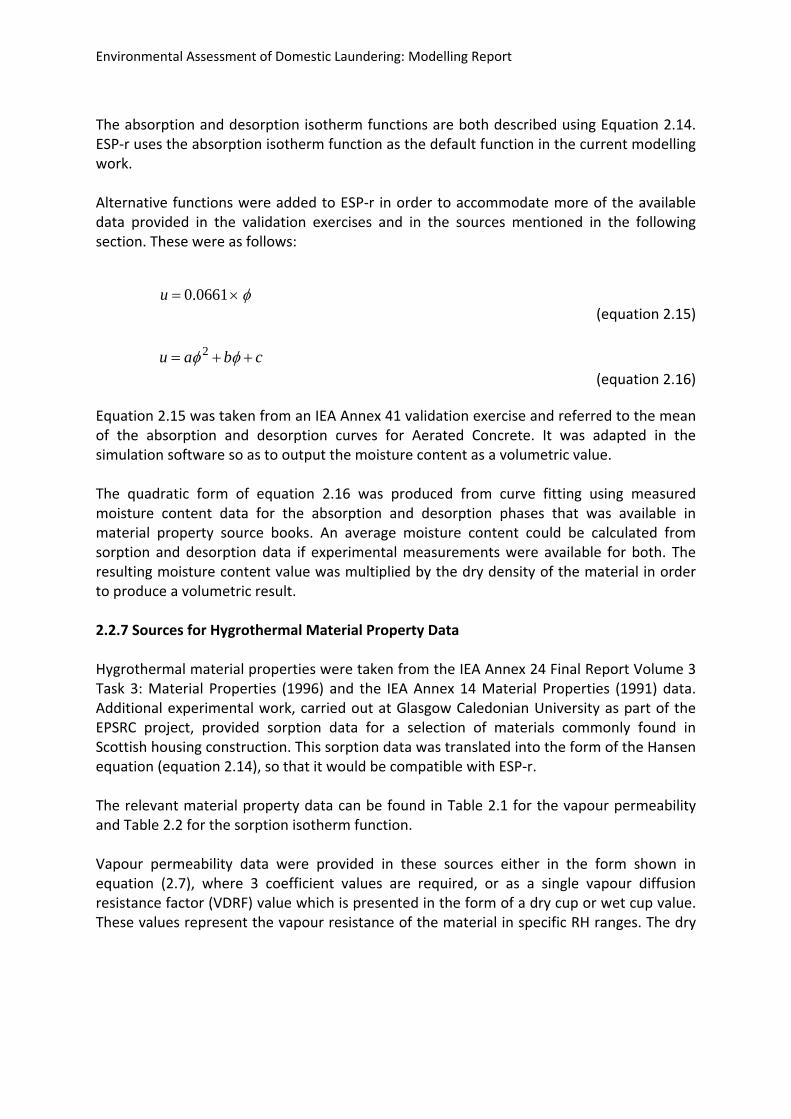
The absorption and desorption isotherm functions are both described using Equation 2.14. ESP‐r uses the absorption isotherm function as the default function in the current modelling work. Alternative functions were added to ESP‐r in order to accommodate more of the available data provided in the validation exercises and in the sources mentioned in the following section. These were as follows:
u 0.0661 (equation 2.15)
cbau 2 (equation 2.16)
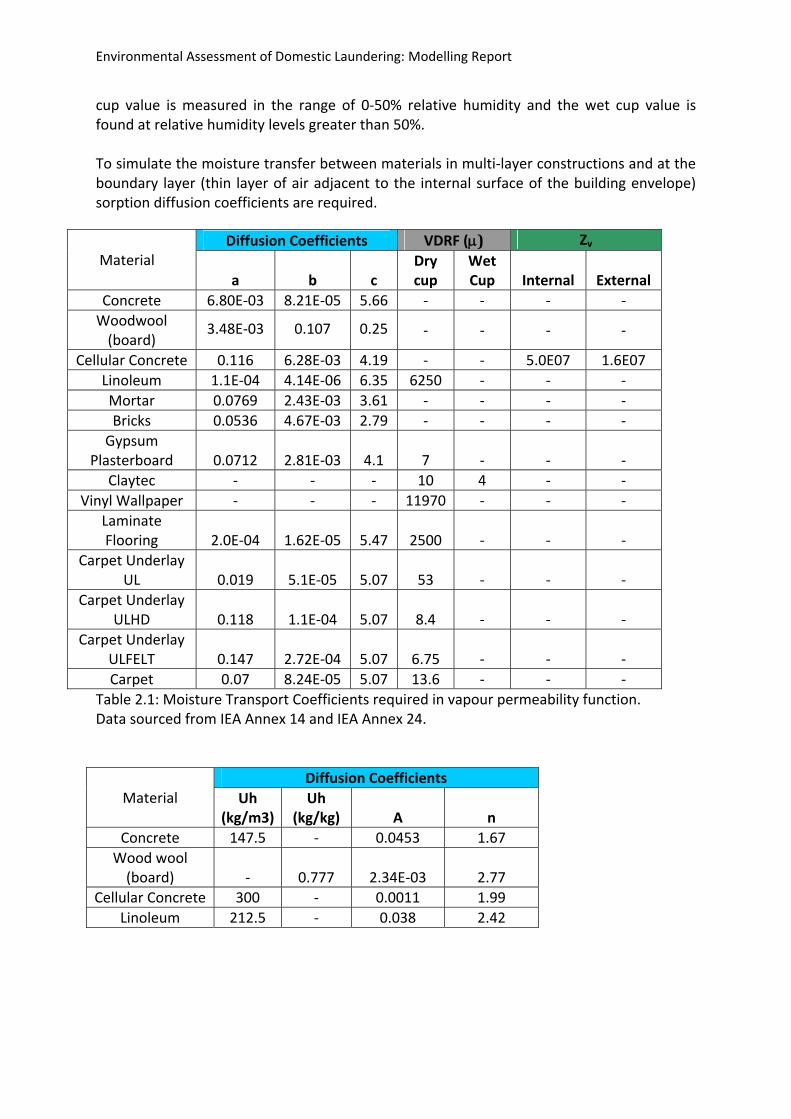
Equation 2.15 was taken from an IEA Annex 41 validation exercise and referred to the mean of the absorption and desorption curves for Aerated Concrete. It was adapted in the simulation software so as to output the moisture content as a volumetric value. The quadratic form of equation 2.16 was produced from curve fitting using measured moisture content data for the absorption and desorption phases that was available in material property source books. An average moisture content could be calculated from sorption and desorption data if experimental measurements were available for both. The resulting moisture content value was multiplied by the dry density of the material in order to produce a volumetric result. 2.2.7 Sources for Hygrothermal Material Property Data Hygrothermal material properties were taken from the IEA Annex 24 Final Report Volume 3 Task 3: Material Properties (1996) and the IEA Annex 14 Material Properties (1991) data. Additional experimental work, carried out at Glasgow Caledonian University as part of the EPSRC project, provided sorption data for a selection of materials commonly found in Scottish housing construction. This sorption data was translated into the form of the Hansen equation (equation 2.14), so that it would be compatible with ESP‐r. The relevant material property data can be found in Table 2.1 for the vapour permeability and Table 2.2 for the sorption isotherm function. Vapour permeability data were provided in these sources either in the form shown in equation (2.7), where 3 coefficient values are required, or as a single vapour diffusion resistance factor (VDRF) value which is presented in the form of a dry cup or wet cup value. These values represent the vapour resistance of the material in specific RH ranges. The dry
Environmental Assessment of Domestic Laundering: Modelling Report
cup value is measured in the range of 0‐50% relative humidity and the wet cup value is found at relative humidity levels greater than 50%. To simulate the moisture transfer between materials in multi‐layer constructions and at the boundary layer (thin layer of air adjacent to the internal surface of the building envelope) sorption diffusion coefficients are required.
Material Diffusion Coefficients VDRF () Zv
a b c Dry cup
Wet Cup Internal External
Concrete 6.80E‐03 8.21E‐05 5.66 ‐ ‐ ‐ ‐
Woodwool (board)
3.48E‐03 0.107 0.25 ‐ ‐ ‐ ‐
Cellular Concrete 0.116 6.28E‐03 4.19 ‐ ‐ 5.0E07 1.6E07
Linoleum 1.1E‐04 4.14E‐06 6.35 6250 ‐ ‐ ‐
Mortar 0.0769 2.43E‐03 3.61 ‐ ‐ ‐ ‐
Bricks 0.0536 4.67E‐03 2.79 ‐ ‐ ‐ ‐
Gypsum Plasterboard 0.0712 2.81E‐03
4.1 7 ‐ ‐ ‐
Claytec ‐ ‐ ‐ 10 4 ‐ ‐
Vinyl Wallpaper ‐ ‐ ‐ 11970 ‐ ‐ ‐
Laminate Flooring 2.0E‐04 1.62E‐05
5.47 2500 ‐ ‐ ‐
Carpet Underlay UL 0.019 5.1E‐05
5.07
53 ‐ ‐ ‐
Carpet Underlay ULHD 0.118 1.1E‐04
5.07
8.4 ‐ ‐ ‐
Carpet Underlay ULFELT 0.147 2.72E‐04
5.07
6.75 ‐ ‐ ‐
Carpet 0.07 8.24E‐05 5.07 13.6 ‐ ‐ ‐
Table 2.1: Moisture Transport Coefficients required in vapour permeability function. Data sourced from IEA Annex 14 and IEA Annex 24.
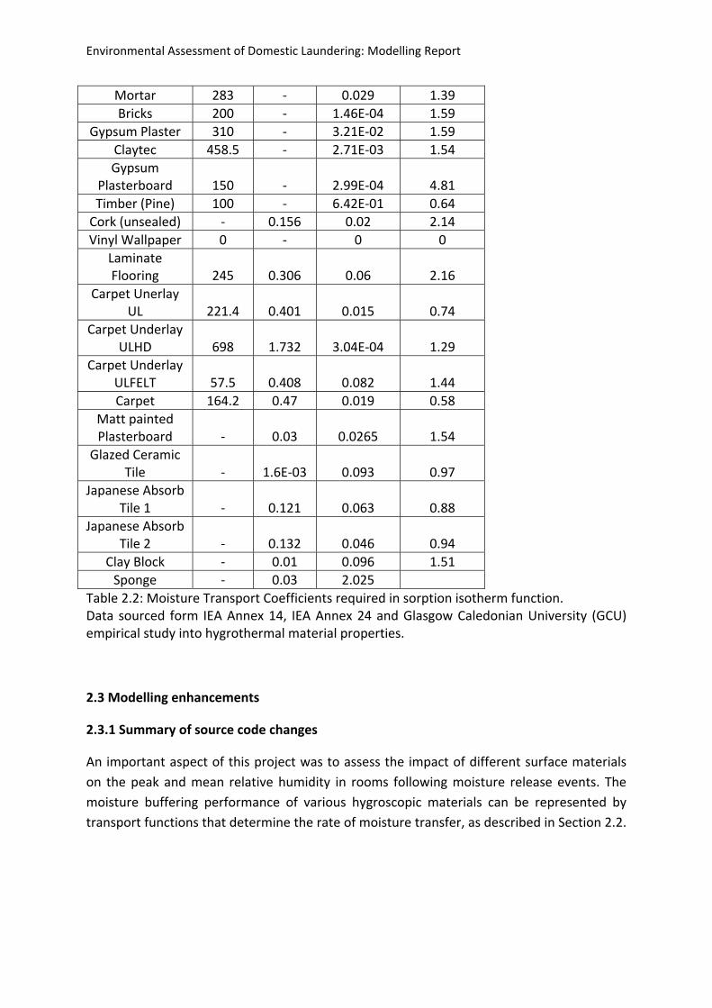
Material Diffusion Coefficients
Uh (kg/m3)
Uh (kg/kg) A n
Concrete 147.5 ‐ 0.0453 1.67
Wood wool (board) ‐
0.777 2.34E‐03 2.77
Cellular Concrete 300 ‐ 0.0011 1.99
Linoleum 212.5 ‐ 0.038 2.42
Environmental Assessment of Domestic Laundering: Modelling Report
Mortar 283 ‐ 0.029 1.39
Bricks 200 ‐ 1.46E‐04 1.59
Gypsum Plaster 310 ‐ 3.21E‐02 1.59
Claytec 458.5 ‐ 2.71E‐03 1.54
Gypsum Plasterboard 150
‐ 2.99E‐04 4.81
Timber (Pine) 100 ‐ 6.42E‐01 0.64
Cork (unsealed) ‐ 0.156 0.02 2.14
Vinyl Wallpaper 0 ‐ 0 0
Laminate Flooring 245
0.306 0.06 2.16
Carpet Unerlay UL 221.4
0.401 0.015 0.74
Carpet Underlay ULHD 698
1.732 3.04E‐04 1.29
Carpet Underlay ULFELT 57.5
0.408 0.082 1.44
Carpet 164.2 0.47 0.019 0.58
Matt painted Plasterboard ‐
0.03 0.0265 1.54
Glazed Ceramic Tile ‐
1.6E‐03 0.093 0.97
Japanese Absorb Tile 1 ‐
0.121 0.063 0.88
Japanese Absorb Tile 2 ‐
0.132 0.046 0.94
Clay Block ‐ 0.01 0.096 1.51
Sponge ‐ 0.03 2.025
Table 2.2: Moisture Transport Coefficients required in sorption isotherm function. Data sourced form IEA Annex 14, IEA Annex 24 and Glasgow Caledonian University (GCU) empirical study into hygrothermal material properties.
2.3 Modelling enhancements
2.3.1 Summary of source code changes
An important aspect of this project was to assess the impact of different surface materials
on the peak and mean relative humidity in rooms following moisture release events. The
moisture buffering performance of various hygroscopic materials can be represented by
transport functions that determine the rate of moisture transfer, as described in Section 2.2.
Environmental Assessment of Domestic Laundering: Modelling Report
The established transport functions included in the moisture modelling module of ESP‐r are
the sorption isotherm function and the vapour permeability. The source code was modified
to enhance the range of functions that can be used to model the behaviour of moisture in
existing housing construction materials.
In addition to the new moisture transport functions entered, experimental data was used to
develop a moisture source model. This model was used to represent wet clothing releasing
moisture into the indoor air, resulting in an increase in relative humidity. This is reported in
Section 2.4
2.3.2 Moisture Transport Functions
Moisture Content
For ESP‐r to calculate the moisture content of a material found in the building envelope
construction, three moisture transport coefficients are required. These coefficients are
determined from curve fitting, using empirical data obtained from the wet and dry cup
tests. Equation 2.13 is used in ESP‐r to calculate the moisture content.
Values for the three transport coefficients specified in the original moisture content
calculation in ESP‐r were taken from IEA Annex 14 and 24 and also supplied by Glasgow
Caledonian University (GCU). Experimental results collected by GCU for a range of materials
were manipulated to provide the data format required by ESP‐r.
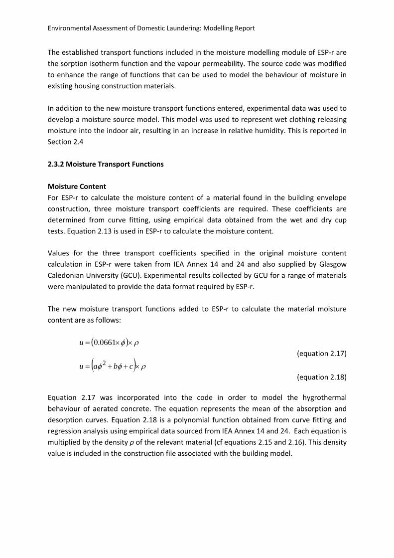
The new moisture transport functions added to ESP‐r to calculate the material moisture
content are as follows:
0661.0u (equation 2.17)
cbau 2 (equation 2.18)
Equation 2.17 was incorporated into the code in order to model the hygrothermal
behaviour of aerated concrete. The equation represents the mean of the absorption and
desorption curves. Equation 2.18 is a polynomial function obtained from curve fitting and
regression analysis using empirical data sourced from IEA Annex 14 and 24. Each equation is
multiplied by the density ρ of the relevant material (cf equations 2.15 and 2.16). This density
value is included in the construction file associated with the building model.
Environmental Assessment of Domestic Laundering: Modelling Report
An index variable was used to indicate which equation should be used with the data for the
particular material.
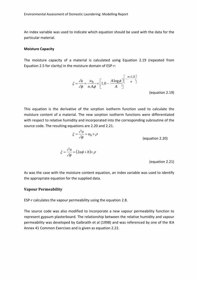
Moisture Capacity
The moisture capacity of a material is calculated using Equation 2.19 (repeated from
Equation 2.5 for clarity) in the moisture domain of ESP‐r:
n
n
h
A
A
An
uu0.1
log0.1
..
(equation 2.19)
This equation is the derivative of the sorption isotherm function used to calculate the
moisture content of a material. The new sorption isotherm functions were differentiated
with respect to relative humidity and incorporated into the corresponding subroutine of the
source code. The resulting equations are 2.20 and 2.21.
hu
u
(equation 2.20)
ba
u2
(equation 2.21)
As was the case with the moisture content equation, an index variable was used to identify
the appropriate equation for the supplied data.
VapourPermeabilityESP‐r calculates the vapour permeabilityusing the equation 2.8.The source code was also modified to incorporate a new vapour permeability function to
represent gypsum plasterboard. The relationship between the relative humidity and vapour
permeability was developed by Galbraith et al (1998) and was referenced by one of the IEA
Annex 41 Common Exercises and is given as equation 2.22.
Environmental Assessment of Domestic Laundering: Modelling Report
1110 ba
(equation 2.22)
Once again, an index was used to indicate the appropriate function for the data.
Air Node Moisture Balance
ESP‐r is able to perform an air node moisture balance, taking into account all sources of
moisture in the modelled zone and exfiltration. Mass flow into the zone is quantified in
terms of the amount of air infiltration and mechanical ventilation (if being modelled) taking
place in the selected zone. This moisture is then added to the moisture that is generated
inside the zone, such as surface evaporation and/or the latent gains injected into the space
(the latent gains being representative of occupant activity, for example). Improvements and
checks were made to the code to ensure that the moisture exchanges at surfaces and
moisture injections into the zones were both included correctly in the moisture balance.
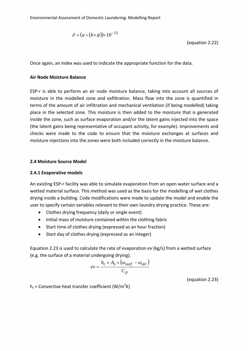
2.4 Moisture Source Model
2.4.1 Evaporative models
An existing ESP‐r facility was able to simulate evaporation from an open water surface and a
wetted material surface. This method was used as the basis for the modelling of wet clothes
drying inside a building. Code modifications were made to update the model and enable the
user to specify certain variables relevant to their own laundry drying practice. These are:
Clothes drying frequency (daily or single event)
Initial mass of moisture contained within the clothing fabric
Start time of clothes drying (expressed as an hour fraction)
Start day of clothes drying (expressed as an integer)
Equation 2.23 is used to calculate the rate of evaporation eν (kg/s) from a wetted surface
(e.g. the surface of a material undergoing drying).
p
airsurfsc
C
Ahev
(equation 2.23)hc = Convective heat transfer coefficient (W/m2K)
Environmental Assessment of Domestic Laundering: Modelling Report
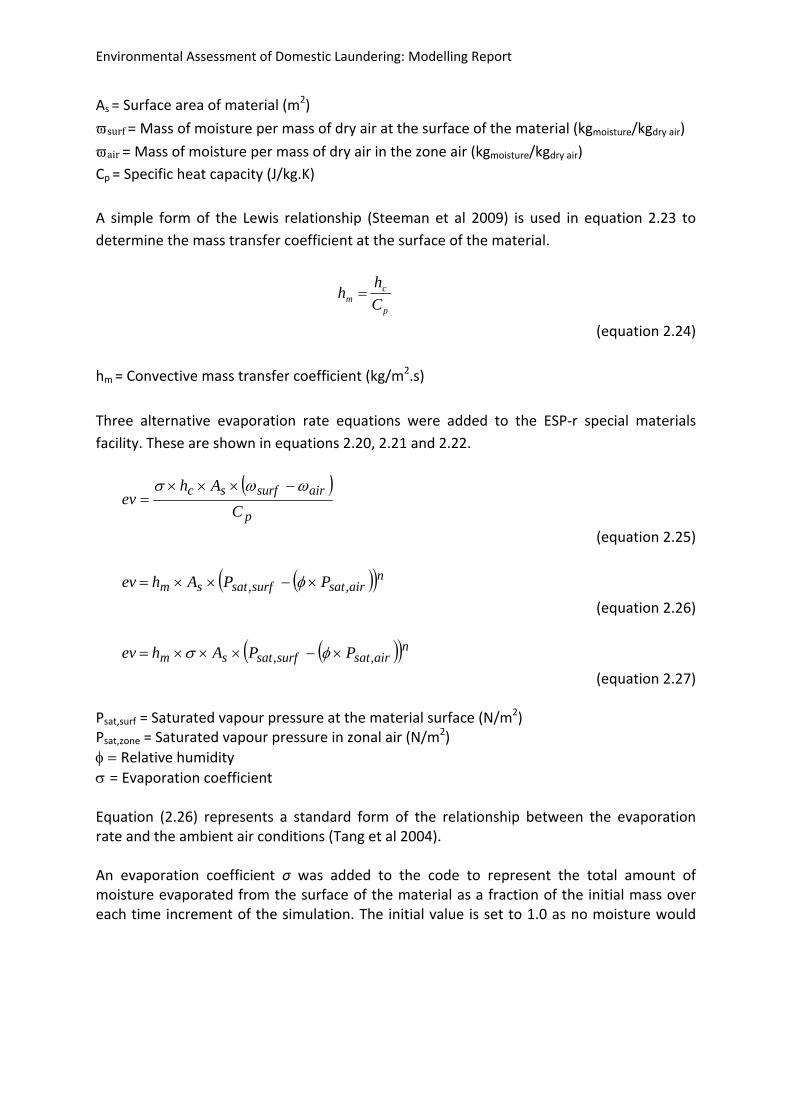
As = Surface area of material (m2)surf=Mass of moisture per mass of dry air at the surface of the material (kgmoisture/kgdry air)
air=Mass of moisture per mass of dry air in the zone air (kgmoisture/kgdry air)
Cp = Specific heat capacity (J/kg.K)
A simple form of the Lewis relationship (Steeman et al 2009) is used in equation 2.23 to
determine the mass transfer coefficient at the surface of the material.
hm hc
Cp
(equation 2.24)
hm = Convective mass transfer coefficient (kg/m2.s)
Three alternative evaporation rate equations were added to the ESP‐r special materials
facility. These are shown in equations 2.20, 2.21 and 2.22.
p
airsurfsc
C
Ahev
(equation 2.25)
nairsatsurfsatsm PPAhev ,,
(equation 2.26)
nairsatsurfsatsm PPAhev ,,
(equation 2.27) Psat,surf = Saturated vapour pressure at the material surface (N/m2) Psat,zone = Saturated vapour pressure in zonal air (N/m
2) Relative humidity
=Evaporation coefficient Equation (2.26) represents a standard form of the relationship between the evaporation rate and the ambient air conditions (Tang et al 2004). An evaporation coefficient σ was added to the code to represent the total amount of moisture evaporated from the surface of the material as a fraction of the initial mass over each time increment of the simulation. The initial value is set to 1.0 as no moisture would
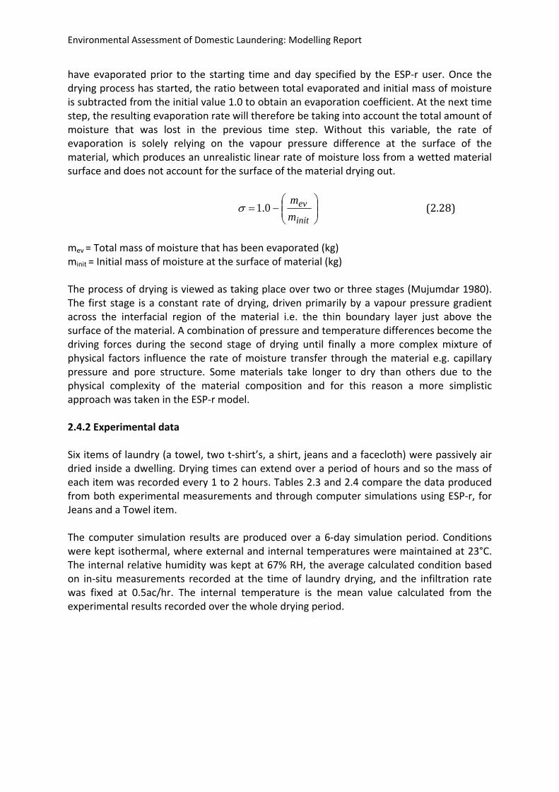
Environmental Assessment of Domestic Laundering: Modelling Report
have evaporated prior to the starting time and day specified by the ESP‐r user. Once the drying process has started, the ratio between total evaporated and initial mass of moisture is subtracted from the initial value 1.0 to obtain an evaporation coefficient. At the next time step, the resulting evaporation rate will therefore be taking into account the total amount of moisture that was lost in the previous time step. Without this variable, the rate of evaporation is solely relying on the vapour pressure difference at the surface of the material, which produces an unrealistic linear rate of moisture loss from a wetted material surface and does not account for the surface of the material drying out.
init
ev
m
m0.1 (2.28)
mev = Total mass of moisture that has been evaporated (kg) minit = Initial mass of moisture at the surface of material (kg) The process of drying is viewed as taking place over two or three stages (Mujumdar 1980). The first stage is a constant rate of drying, driven primarily by a vapour pressure gradient across the interfacial region of the material i.e. the thin boundary layer just above the surface of the material. A combination of pressure and temperature differences become the driving forces during the second stage of drying until finally a more complex mixture of physical factors influence the rate of moisture transfer through the material e.g. capillary pressure and pore structure. Some materials take longer to dry than others due to the physical complexity of the material composition and for this reason a more simplistic approach was taken in the ESP‐r model. 2.4.2 Experimental data Six items of laundry (a towel, two t‐shirt’s, a shirt, jeans and a facecloth) were passively air dried inside a dwelling. Drying times can extend over a period of hours and so the mass of each item was recorded every 1 to 2 hours. Tables 2.3 and 2.4 compare the data produced from both experimental measurements and through computer simulations using ESP‐r, for Jeans and a Towel item. The computer simulation results are produced over a 6‐day simulation period. Conditions were kept isothermal, where external and internal temperatures were maintained at 23°C. The internal relative humidity was kept at 67% RH, the average calculated condition based on in‐situ measurements recorded at the time of laundry drying, and the infiltration rate was fixed at 0.5ac/hr. The internal temperature is the mean value calculated from the experimental results recorded over the whole drying period.
Environmental Assessment of Domestic Laundering: Modelling Report
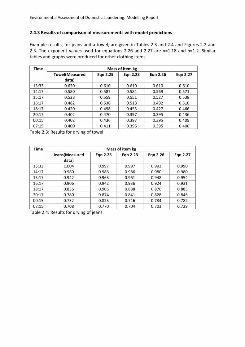
2.4.3 Results of comparison of measurements with model predictions Example results, for jeans and a towel, are given in Tables 2.3 and 2.4 and Figures 2.2 and 2.3. The exponent values used for equations 2.26 and 2.27 are n=1.18 and n=1.2. Similar tables and graphs were produced for other clothing items. Time Mass of item kg
Towel(Measured data)
Eqn 2.25 Eqn 2.23 Eqn 2.26 Eqn 2.27
13:33 0.620 0.610 0.610 0.610 0.610
14:17 0.580 0.587 0.584 0.569 0.571
15:17 0.528 0.559 0.551 0.527 0.538
16:17 0.482 0.536 0.518 0.492 0.510
18:17 0.420 0.498 0.453 0.427 0.466
20:17 0.402 0.470 0.397 0.395 0.436
00:15 0.402 0.436 0.397 0.395 0.409
07:15 0.400 0.411 0.396 0.395 0.400
Table 2.3: Results for drying of towel
Time Mass of item kg
Jeans(Measured data)
Eqn 2.25 Eqn 2.23 Eqn 2.26 Eqn 2.27
13:33 1.004 0.997 0.997 0.992 0.990
14:17 0.980 0.986 0.986 0.980 0.980
15:17 0.942 0.963 0.961 0.948 0.954
16:17 0.906 0.942 0.936 0.924 0.931
18:17 0.836 0.905 0.888 0.876 0.885
20:17 0.780 0.874 0.841 0.828 0.845
00:15 0.732 0.825 0.746 0.734 0.782
07:15 0.708 0.770 0.704 0.703 0.729
Table 2.4: Results for drying of jeans
Environmental Assessment of Domestic Laundering: Modelling Report
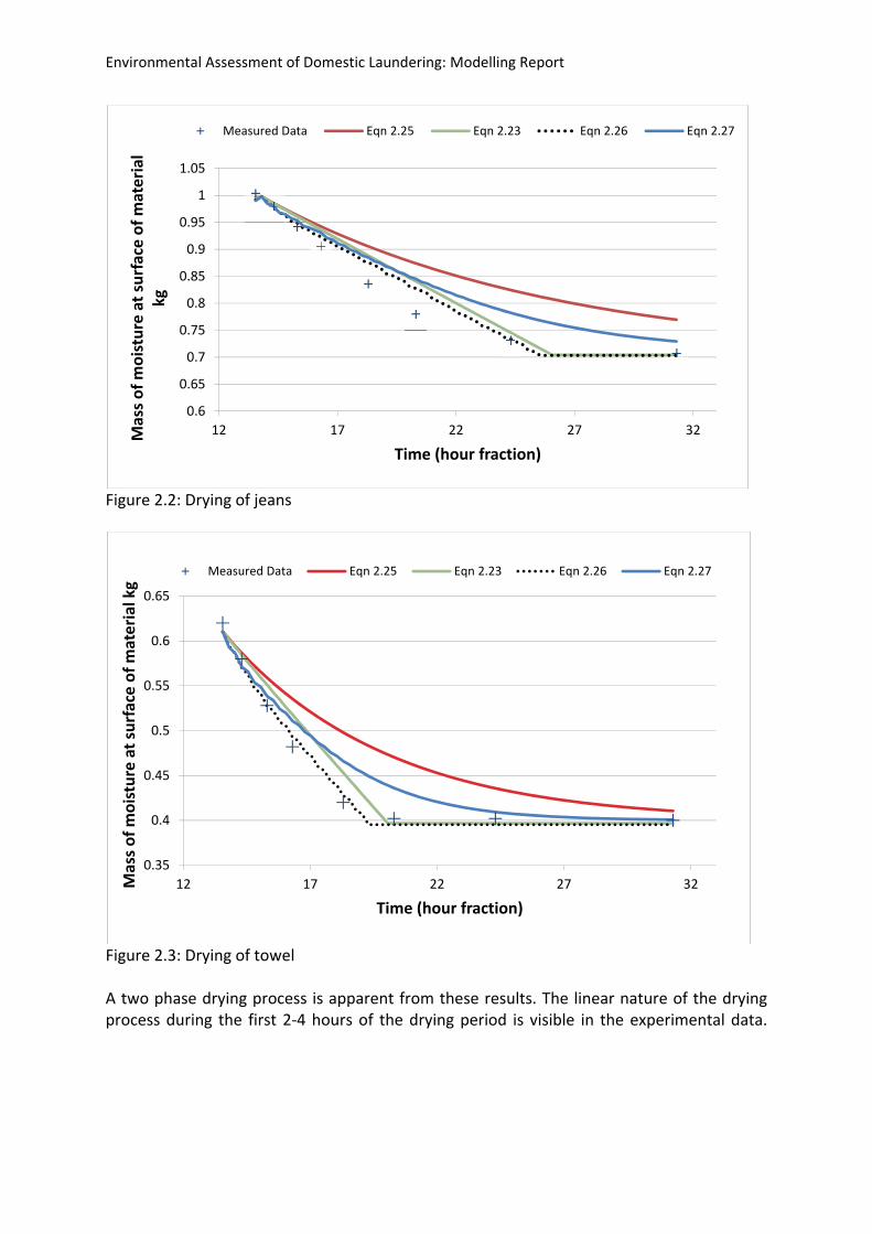
Figure 2.2: Drying of jeans
Figure 2.3: Drying of towel A two phase drying process is apparent from these results. The linear nature of the drying process during the first 2‐4 hours of the drying period is visible in the experimental data.
0.6
0.65
0.7
0.75
0.8
0.85
0.9
0.95
1
1.05
12 17 22 27 32Mass of moisture at surface of material
kg
Time (hour fraction)
Measured Data Eqn 2.25 Eqn 2.23 Eqn 2.26 Eqn 2.27
0.35
0.4
0.45
0.5
0.55
0.6
0.65
12 17 22 27 32Mass of moisture at surface of material kg
Time (hour fraction)
Measured Data Eqn 2.25 Eqn 2.23 Eqn 2.26 Eqn 2.27
Environmental Assessment of Domestic Laundering: Modelling Report
Predicted results from ESP‐r’s evaporation rate calculations show reasonable correlation with experimental data in most clothing items during this initial drying period. The non‐linear rate of decay is observed after this initial period until the clothing items have reached their dry weight. The agreement is poorer for equations 2.25 and 2.27. The predicted drying curves showed a much longer time needed for the items to reach their dry weight in comparison to the measured results ‐ this was the case for most items. The most prominent differences are seen when modelling the towel and jeans. This is possibly due to the more complex material structure of these items that creates greater resistance to mass transfer and the combined effect of vapour and liquid transfer processes occurring in this type of material. Although more experimental data is needed to improve the models for moisture release, it was considered that the models developed were adequate to represent the moisture release within this project.
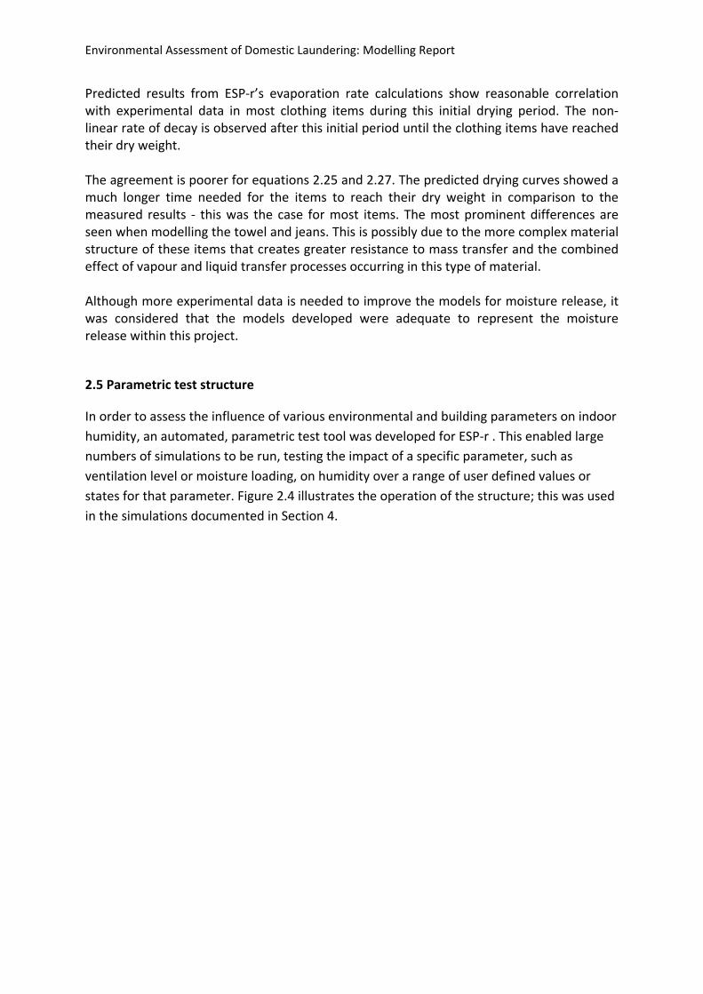
2.5 Parametric test structure
In order to assess the influence of various environmental and building parameters on indoor
humidity, an automated, parametric test tool was developed for ESP‐r . This enabled large
numbers of simulations to be run, testing the impact of a specific parameter, such as
ventilation level or moisture loading, on humidity over a range of user defined values or
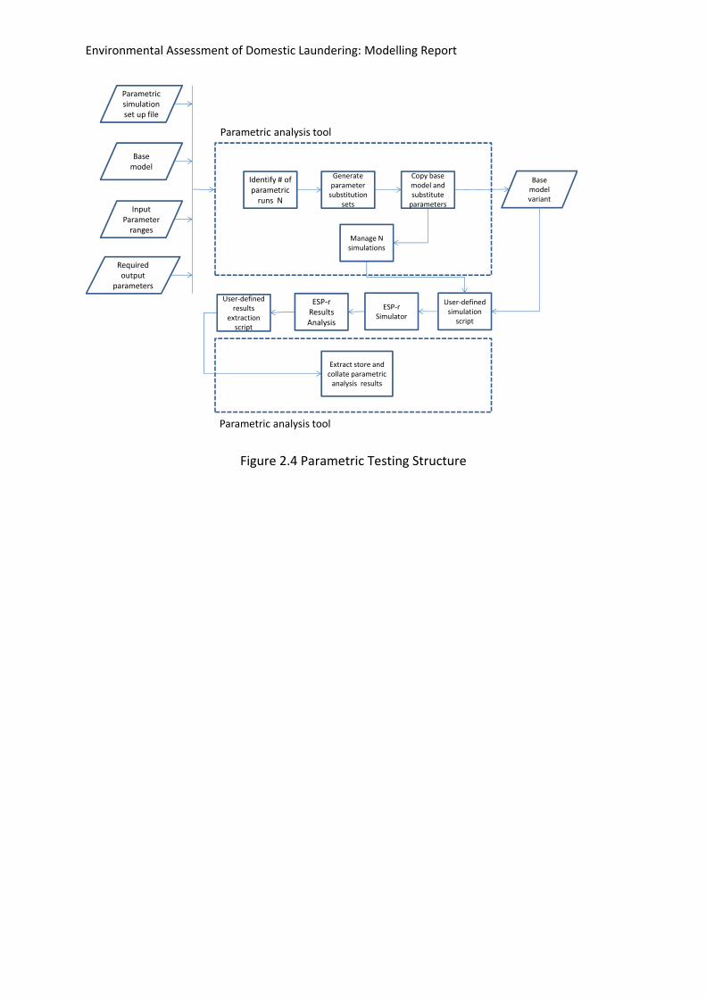
states for that parameter. Figure 2.4 illustrates the operation of the structure; this was used
in the simulations documented in Section 4.
Environmental Assessment of Domestic Laundering: Modelling Report
Figure 2.4 Parametric Testing Structure
ESP‐r Results Analysis
Identify # of parametric runs N
User‐defined simulation script
User‐defined results
extraction script
ESP‐r Simulator
Parametric simulation set up file
Generate parameter substitution
sets
Base model variant
Manage N simulations
Extract store and collate parametric analysis results
Copy base model and substitute parameters
Base model
Input Parameter ranges
Required output
parameters
Parametric analysis tool
Parametric analysis tool
Environmental Assessment of Domestic Laundering: Modelling Report
3. Validation
The ability of ESP‐r to model moisture transfer was tested using a number of validation tests
developed within IEA Annex 41 Subtask 1 (Woloszyn and Rode 2007). Also, a number of
cyclic tests were conducted by Glasgow Caledonian University within the scope of this
project.
3.1 IEA 41 validation tests
Over the last few decades, there has been continuing development and increased use of
heat, air and moisture (HAM) modelling software tools in the building services and design
industries. A vast majority of these tools are able to simulate the behaviour of heat, air and
moisture at the air point in a building. However, the need to develop reliable and accurate
modelling of the hygrothermal interactions at the surface of the material and within the
envelope construction is growing rapidly.
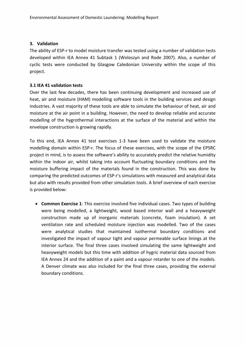
To this end, IEA Annex 41 test exercises 1‐3 have been used to validate the moisture
modelling domain within ESP‐r. The focus of these exercises, with the scope of the EPSRC
project in mind, is to assess the software’s ability to accurately predict the relative humidity
within the indoor air, whilst taking into account fluctuating boundary conditions and the
moisture buffering impact of the materials found in the construction. This was done by
comparing the predicted outcomes of ESP‐r’s simulations with measured and analytical data
but also with results provided from other simulation tools. A brief overview of each exercise
is provided below:
Common Exercise 1: This exercise involved five individual cases. Two types of building
were being modelled, a lightweight, wood based interior wall and a heavyweight
construction made up of inorganic materials (concrete, foam insulation). A set
ventilation rate and scheduled moisture injection was modelled. Two of the cases
were analytical studies that maintained isothermal boundary conditions and
investigated the impact of vapour tight and vapour permeable surface linings at the
interior surface. The final three cases involved simulating the same lightweight and
heavyweight models but this time with addition of hygric material data sourced from
IEA Annex 24 and the addition of a paint and a vapour retarder to one of the models.
A Denver climate was also included for the final three cases, providing the external
boundary conditions.
Environmental Assessment of Domestic Laundering: Modelling Report
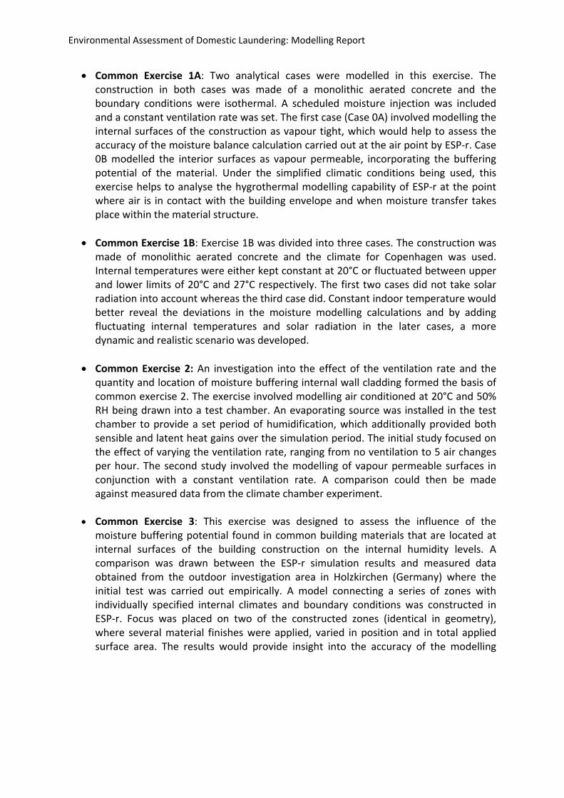
Common Exercise 1A: Two analytical cases were modelled in this exercise. The construction in both cases was made of a monolithic aerated concrete and the boundary conditions were isothermal. A scheduled moisture injection was included and a constant ventilation rate was set. The first case (Case 0A) involved modelling the internal surfaces of the construction as vapour tight, which would help to assess the accuracy of the moisture balance calculation carried out at the air point by ESP‐r. Case 0B modelled the interior surfaces as vapour permeable, incorporating the buffering potential of the material. Under the simplified climatic conditions being used, this exercise helps to analyse the hygrothermal modelling capability of ESP‐r at the point where air is in contact with the building envelope and when moisture transfer takes place within the material structure.
Common Exercise 1B: Exercise 1B was divided into three cases. The construction was made of monolithic aerated concrete and the climate for Copenhagen was used. Internal temperatures were either kept constant at 20°C or fluctuated between upper and lower limits of 20°C and 27°C respectively. The first two cases did not take solar radiation into account whereas the third case did. Constant indoor temperature would better reveal the deviations in the moisture modelling calculations and by adding fluctuating internal temperatures and solar radiation in the later cases, a more dynamic and realistic scenario was developed.
Common Exercise 2: An investigation into the effect of the ventilation rate and the quantity and location of moisture buffering internal wall cladding formed the basis of common exercise 2. The exercise involved modelling air conditioned at 20°C and 50% RH being drawn into a test chamber. An evaporating source was installed in the test chamber to provide a set period of humidification, which additionally provided both sensible and latent heat gains over the simulation period. The initial study focused on the effect of varying the ventilation rate, ranging from no ventilation to 5 air changes per hour. The second study involved the modelling of vapour permeable surfaces in conjunction with a constant ventilation rate. A comparison could then be made against measured data from the climate chamber experiment.
Common Exercise 3: This exercise was designed to assess the influence of the
moisture buffering potential found in common building materials that are located at internal surfaces of the building construction on the internal humidity levels. A comparison was drawn between the ESP‐r simulation results and measured data obtained from the outdoor investigation area in Holzkirchen (Germany) where the initial test was carried out empirically. A model connecting a series of zones with individually specified internal climates and boundary conditions was constructed in ESP‐r. Focus was placed on two of the constructed zones (identical in geometry), where several material finishes were applied, varied in position and in total applied surface area. The results would provide insight into the accuracy of the modelling
Environmental Assessment of Domestic Laundering: Modelling Report
process in determining internal relative humidity levels using dynamic external boundary conditions.
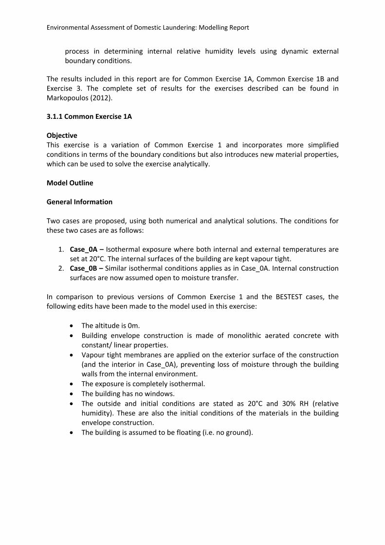
The results included in this report are for Common Exercise 1A, Common Exercise 1B and Exercise 3. The complete set of results for the exercises described can be found in Markopoulos (2012). 3.1.1 Common Exercise 1A Objective This exercise is a variation of Common Exercise 1 and incorporates more simplified conditions in terms of the boundary conditions but also introduces new material properties, which can be used to solve the exercise analytically. Model Outline General Information Two cases are proposed, using both numerical and analytical solutions. The conditions for these two cases are as follows:
1. Case_0A – Isothermal exposure where both internal and external temperatures are set at 20°C. The internal surfaces of the building are kept vapour tight.
2. Case_0B – Similar isothermal conditions applies as in Case_0A. Internal construction surfaces are now assumed open to moisture transfer.
In comparison to previous versions of Common Exercise 1 and the BESTEST cases, the following edits have been made to the model used in this exercise:
The altitude is 0m.
Building envelope construction is made of monolithic aerated concrete with constant/ linear properties.
Vapour tight membranes are applied on the exterior surface of the construction (and the interior in Case_0A), preventing loss of moisture through the building walls from the internal environment.
The exposure is completely isothermal.
The building has no windows.
The outside and initial conditions are stated as 20°C and 30% RH (relative humidity). These are also the initial conditions of the materials in the building envelope construction.
The building is assumed to be floating (i.e. no ground).
Environmental Assessment of Domestic Laundering: Modelling Report
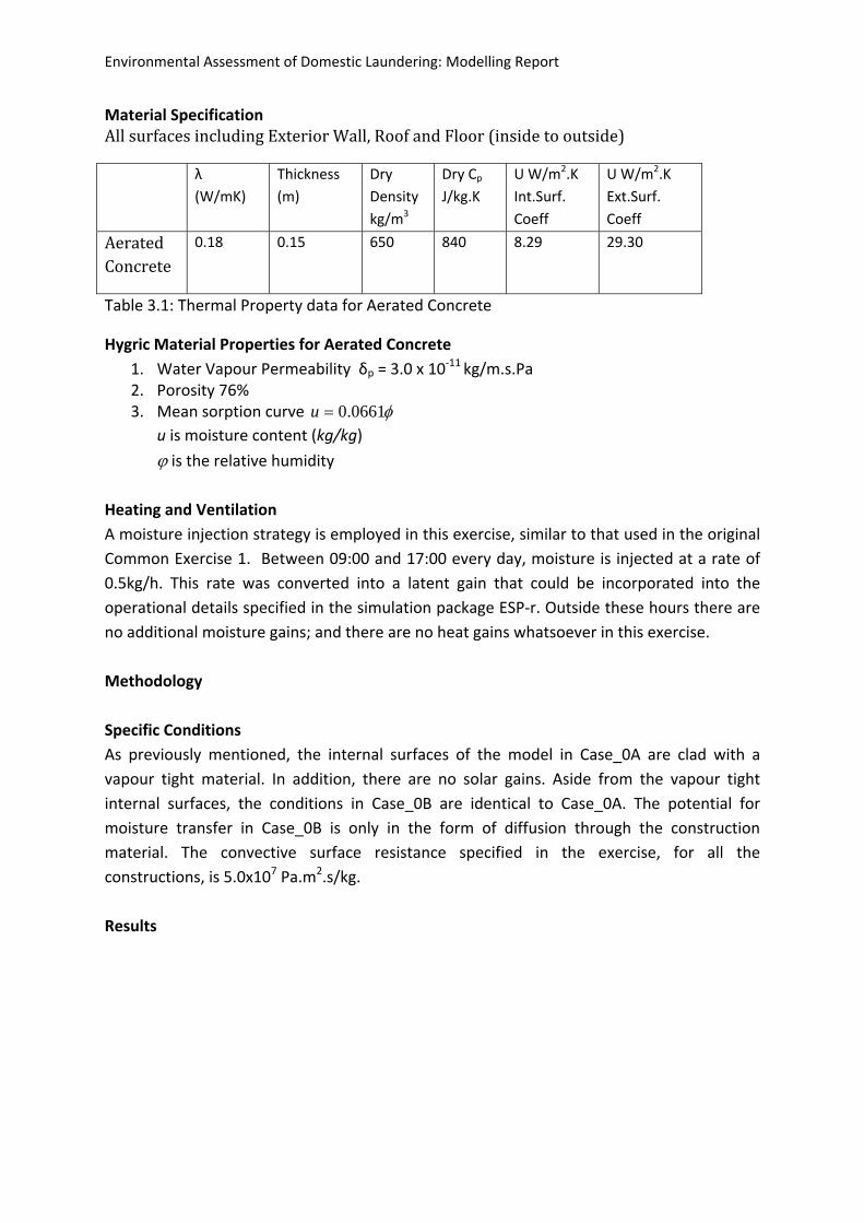
Material Specification AllsurfacesincludingExteriorWall,RoofandFloor(insidetooutside)
λ
(W/mK)
Thickness
(m)
Dry
Density
kg/m3
Dry Cp
J/kg.K
U W/m2.K
Int.Surf.
Coeff
U W/m2.K
Ext.Surf.
Coeff
AeratedConcrete
0.18 0.15 650 840 8.29 29.30
Table 3.1: Thermal Property data for Aerated Concrete
Hygric Material Properties for Aerated Concrete
1. Water Vapour Permeability δp = 3.0 x 10‐11 kg/m.s.Pa
2. Porosity 76% 3. Mean sorption curve 0661.0u
u is moisture content (kg/kg)
is the relative humidity
Heating and Ventilation
A moisture injection strategy is employed in this exercise, similar to that used in the original
Common Exercise 1. Between 09:00 and 17:00 every day, moisture is injected at a rate of
0.5kg/h. This rate was converted into a latent gain that could be incorporated into the
operational details specified in the simulation package ESP‐r. Outside these hours there are
no additional moisture gains; and there are no heat gains whatsoever in this exercise.
Methodology
Specific Conditions
As previously mentioned, the internal surfaces of the model in Case_0A are clad with a
vapour tight material. In addition, there are no solar gains. Aside from the vapour tight
internal surfaces, the conditions in Case_0B are identical to Case_0A. The potential for
moisture transfer in Case_0B is only in the form of diffusion through the construction
material. The convective surface resistance specified in the exercise, for all the
constructions, is 5.0x10⁷ Pa.m2.s/kg.
Results
Environmental Assessment of Domestic Laundering: Modelling Report
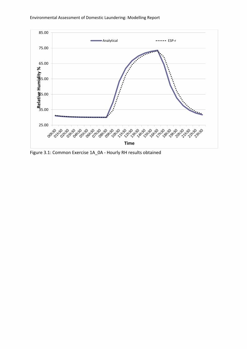
Figure 3.1: Common Exercise 1A_0A ‐ Hourly RH results obtained
25.00
35.00
45.00
55.00
65.00
75.00
85.00
Relative Humidity %
Time
Analytical ESP‐r
Environmental Assessment of Domestic Laundering: Modelling Report
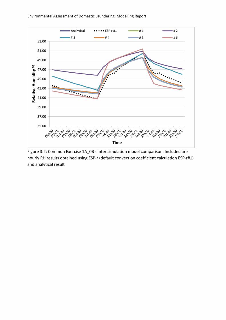
Figure 3.2: Common Exercise 1A_0B ‐ Inter simulation model comparison. Included are
hourly RH results obtained using ESP‐r (default convection coefficient calculation ESP‐r#1)
and analytical result
35.00
37.00
39.00
41.00
43.00
45.00
47.00
49.00
51.00
53.00
Relative Humidity %
Time
Analytical ESP‐r #1 # 1 # 2
# 3 # 4 # 5 # 6
Environmental Assessment of Domestic Laundering: Modelling Report
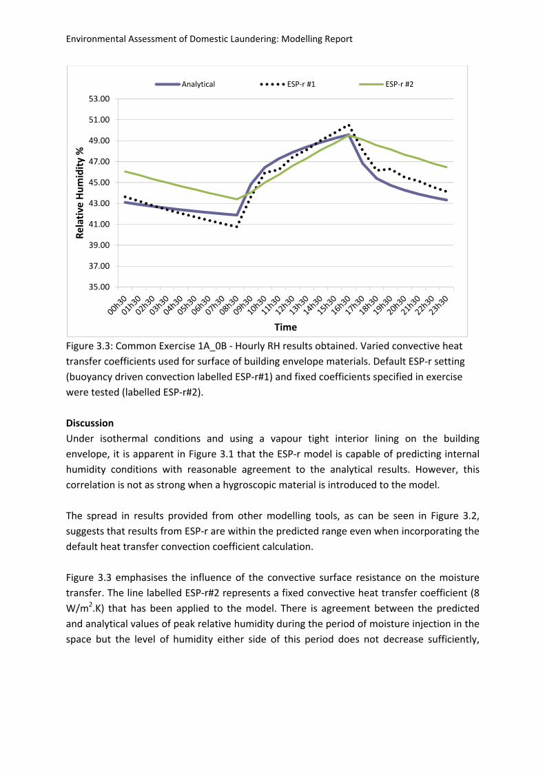
Figure 3.3: Common Exercise 1A_0B ‐ Hourly RH results obtained. Varied convective heat
transfer coefficients used for surface of building envelope materials. Default ESP‐r setting
(buoyancy driven convection labelled ESP‐r#1) and fixed coefficients specified in exercise
were tested (labelled ESP‐r#2).
Discussion
Under isothermal conditions and using a vapour tight interior lining on the building
envelope, it is apparent in Figure 3.1 that the ESP‐r model is capable of predicting internal
humidity conditions with reasonable agreement to the analytical results. However, this
correlation is not as strong when a hygroscopic material is introduced to the model.
The spread in results provided from other modelling tools, as can be seen in Figure 3.2,
suggests that results from ESP‐r are within the predicted range even when incorporating the
default heat transfer convection coefficient calculation.
Figure 3.3 emphasises the influence of the convective surface resistance on the moisture
transfer. The line labelled ESP‐r#2 represents a fixed convective heat transfer coefficient (8
W/m2.K) that has been applied to the model. There is agreement between the predicted
and analytical values of peak relative humidity during the period of moisture injection in the
space but the level of humidity either side of this period does not decrease sufficiently,
35.00
37.00
39.00
41.00
43.00
45.00
47.00
49.00
51.00
53.00
Relative Humidity %
Time
Analytical ESP‐r #1 ESP‐r #2
Environmental Assessment of Domestic Laundering: Modelling Report
possibly due to the release of moisture back into the space from the material during the
desorption phase, which will be driven by the vapour pressure gradient created at the
surface when the moisture in the air is removed by the ventilation.
The default setting for calculating the convective heat transfer coefficient in ESP‐r is
buoyancy controlled, which considers the variations in temperature at a point to calculate
this value. The line labelled ESP‐r#1 in Figure 3.3 displays the results produced when using
this assumption. Peak relative humidity during the moisture injection period is slightly over
estimated, indicating that a reduced value for the surface heat transfer coefficient has been
calculated resulting in a decrease in the potential moisture transfer occurring at the surface.
The reasonable correlation between the predicted and calculated analytical values is more
likely due to the effect of ventilation in the space.
Conclusion
This exercise introduced more simplified environmental conditions and new material
properties into ESP‐r. The initial part of the exercise did not consider the buffering impact of
the envelope material on the internal relative humidity. The focus was simply on modelling
the internal relative humidity correctly. Simulation results produced when using a vapour
tight internal surface material showed good agreement when compared to analytical
results, emphasising the accuracy of the internal air moisture balance being carried out by
ESP‐r under isothermal conditions. The second study looked at the impact of modelling the
moisture buffering effect of the concrete construction. Reasonable agreement was achieved
again between the ESP‐r output and analytical results.
3.1.2 Common Exercise 1B
Objective
This exercise further develops the original BESTEST model, which was initially revised in Common Exercise 0 and 1. Analysis of the indoor and building envelope moisture conditions
are carried out focusing on indoor relative humidity. The construction of the model was
simplified after initial uncertainties were observed in Common Exercise 1. The climate of
Copenhagen was used for these simulations. There are 3 cases designed for the purposes of
testing the transient moisture behaviour.
Methodology
Specific Cases looked at were as follows.
Environmental Assessment of Domestic Laundering: Modelling Report
1. Case ‘20°C, no external radiation’, where the influence of the solar radiation is
neglected and where constant indoor temperature better reveals the deviations in
moisture calculations.
2. Case ’20 to 27°C, no external radiation’, which is a more realistic case but still without
solar and long wave radiation.
3. Case ’20 to 27°C’, now with solar and long wave radiation through the windows and
on the external opaque surfaces.
Model Specification
The location is Copenhagen (altitude: 5m, latitude: 55°37’ north, longitude: 12°40’ east). The
building is constructed entirely out of monolithic aerated concrete and every surface is
subject to the same outdoor boundary conditions, including the floor. No coatings or
membranes are applied to any face.
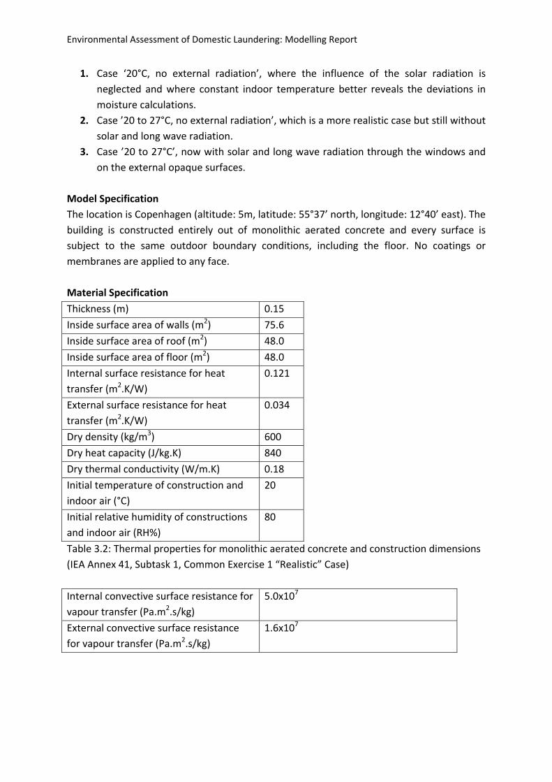
Material Specification
Thickness (m) 0.15
Inside surface area of walls (m2) 75.6
Inside surface area of roof (m2) 48.0
Inside surface area of floor (m2) 48.0
Internal surface resistance for heat
transfer (m2.K/W)
0.121
External surface resistance for heat
transfer (m2.K/W)
0.034
Dry density (kg/m3) 600
Dry heat capacity (J/kg.K) 840
Dry thermal conductivity (W/m.K) 0.18
Initial temperature of construction and
indoor air (°C)
20
Initial relative humidity of constructions
and indoor air (RH%)
80
Table 3.2: Thermal properties for monolithic aerated concrete and construction dimensions
(IEA Annex 41, Subtask 1, Common Exercise 1 “Realistic” Case)
Internal convective surface resistance for
vapour transfer (Pa.m2.s/kg)
5.0x10⁷
External convective surface resistance
for vapour transfer (Pa.m2.s/kg)
1.6x10⁷
Environmental Assessment of Domestic Laundering: Modelling Report
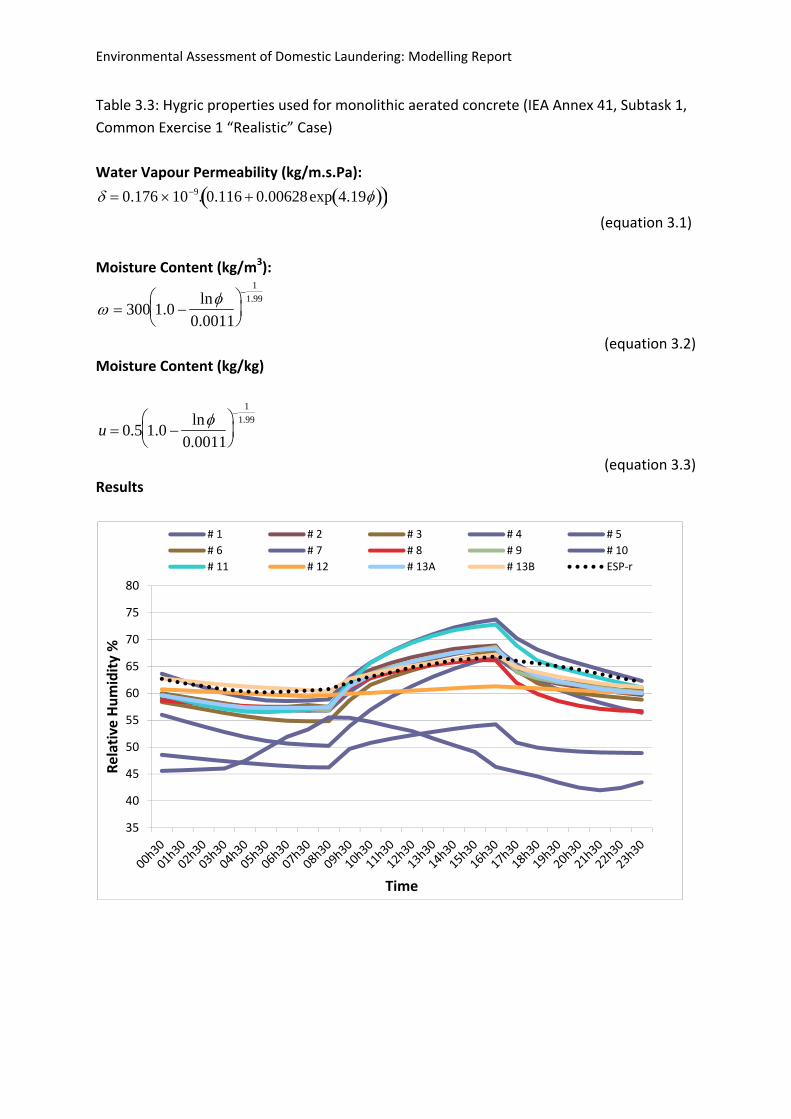
Table 3.3: Hygric properties used for monolithic aerated concrete (IEA Annex 41, Subtask 1,
Common Exercise 1 “Realistic” Case)
Water Vapour Permeability (kg/m.s.Pa):
0.176 109. 0.116 0.00628exp 4.19 (equation 3.1)
Moisture Content (kg/m3):
300 1.0 ln
0.0011
1
1.99
(equation 3.2)
Moisture Content (kg/kg)
u 0.5 1.0 ln
0.0011
1
1.99
(equation 3.3)
Results
35
40
45
50
55
60
65
70
75
80
Relative Humidity %
Time
# 1 # 2 # 3 # 4 # 5
# 6 # 7 # 8 # 9 # 10
# 11 # 12 # 13A # 13B ESP‐r
Environmental Assessment of Domestic Laundering: Modelling Report
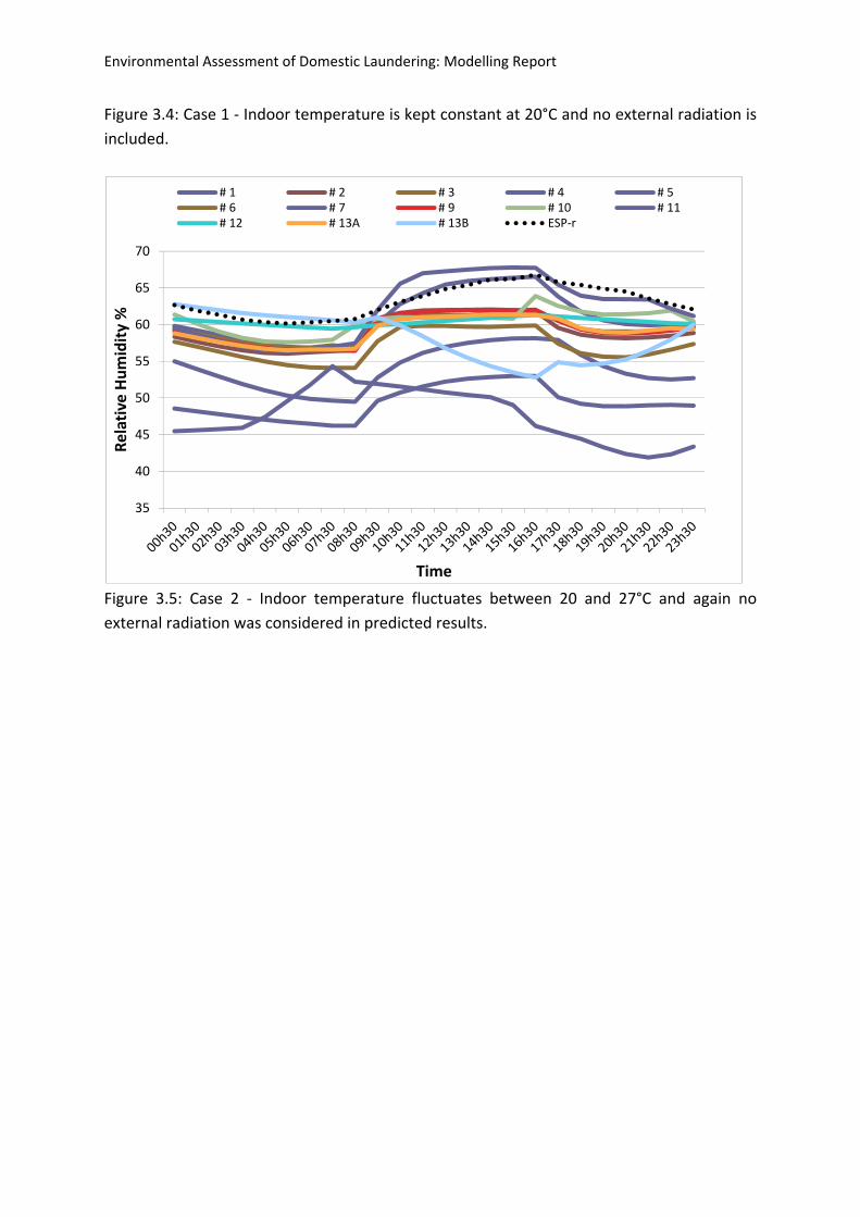
Figure 3.4: Case 1 ‐ Indoor temperature is kept constant at 20°C and no external radiation is
included.
Figure 3.5: Case 2 ‐ Indoor temperature fluctuates between 20 and 27°C and again no
external radiation was considered in predicted results.
35
40
45
50
55
60
65
70
Relative Humidity %
Time
# 1 # 2 # 3 # 4 # 5# 6 # 7 # 9 # 10 # 11# 12 # 13A # 13B ESP‐r
Environmental Assessment of Domestic Laundering: Modelling Report
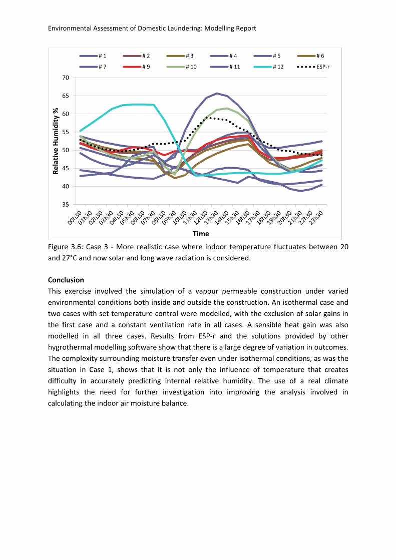
Figure 3.6: Case 3 ‐ More realistic case where indoor temperature fluctuates between 20
and 27°C and now solar and long wave radiation is considered.
Conclusion
This exercise involved the simulation of a vapour permeable construction under varied
environmental conditions both inside and outside the construction. An isothermal case and
two cases with set temperature control were modelled, with the exclusion of solar gains in
the first case and a constant ventilation rate in all cases. A sensible heat gain was also
modelled in all three cases. Results from ESP‐r and the solutions provided by other
hygrothermal modelling software show that there is a large degree of variation in outcomes.
The complexity surrounding moisture transfer even under isothermal conditions, as was the
situation in Case 1, shows that it is not only the influence of temperature that creates
difficulty in accurately predicting internal relative humidity. The use of a real climate
highlights the need for further investigation into improving the analysis involved in
calculating the indoor air moisture balance.
35
40
45
50
55
60
65
70
Relative Humidity %
Time
# 1 # 2 # 3 # 4 # 5 # 6
# 7 # 9 # 10 # 11 # 12 ESP‐r
Environmental Assessment of Domestic Laundering: Modelling Report
3.1.3 Common Exercise 3
ObjectiveThis exercise was designed to observe if the moisture buffering effect of common building
materials, positioned at the internal face of the building envelope, influence the internal
humidity levels and to what extent, using performance predictions produced by simulation
tools. A comparison is then drawn between the simulation results and measured data
obtained from the outdoor investigation area in Holzkirchen (Germany) where the same test
was carried out empirically. A model connecting a series of zones with individually specified
internal climates and boundary conditions was constructed using the building simulation
tool called ESP‐r. Focus was placed on two of the constructed zones (identical in geometry),
where several material finishes were applied, varied in position and the total applied surface
area. The results provide insight into the accuracy of the modelling process in determining
internal climate conditions and energy consumption under real conditions.
Methodology
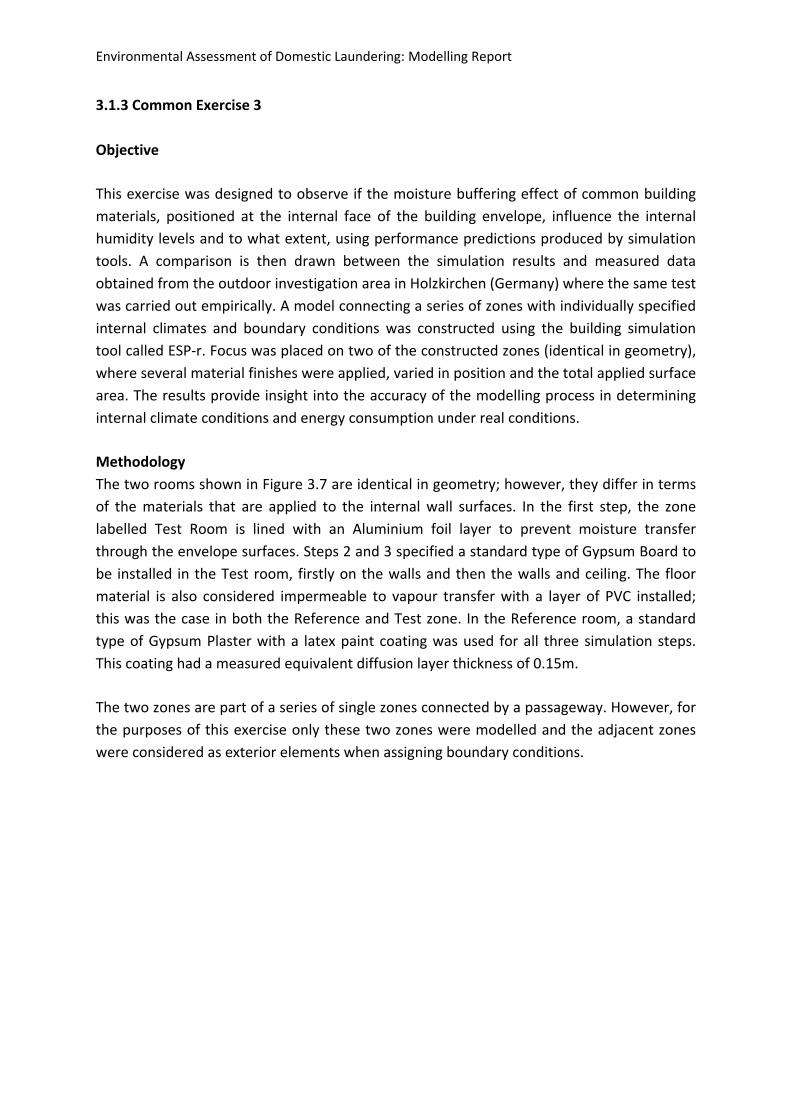
The two rooms shown in Figure 3.7 are identical in geometry; however, they differ in terms
of the materials that are applied to the internal wall surfaces. In the first step, the zone
labelled Test Room is lined with an Aluminium foil layer to prevent moisture transfer
through the envelope surfaces. Steps 2 and 3 specified a standard type of Gypsum Board to
be installed in the Test room, firstly on the walls and then the walls and ceiling. The floor
material is also considered impermeable to vapour transfer with a layer of PVC installed;
this was the case in both the Reference and Test zone. In the Reference room, a standard
type of Gypsum Plaster with a latex paint coating was used for all three simulation steps.
This coating had a measured equivalent diffusion layer thickness of 0.15m.
The two zones are part of a series of single zones connected by a passageway. However, for
the purposes of this exercise only these two zones were modelled and the adjacent zones
were considered as exterior elements when assigning boundary conditions.
Environmental Assessment of Domestic Laundering: Modelling Report
Figure 3.7: Overview of zone floor plan
The temperature in both Reference and Test zone was maintained at 200C using a basic
heating controller system existing in ESP‐r. The maximum power output from this heating
method was kept at 1kW as was specified in the exercise.
One modelling parameter differing between the two zones was the infiltration rate. Due to
surface defects and natural leakage through joints in the buildings construction, masking
tape was used to seal these sources of uncontrolled airflow. A ventilation system was
applied to the Reference and Test zones after tracer gas tests were carried out to calculate
the air change rate during operational hours. The results showed an air change rate of 0.63
for the Reference room and 0.66 ac/h for the Test room.
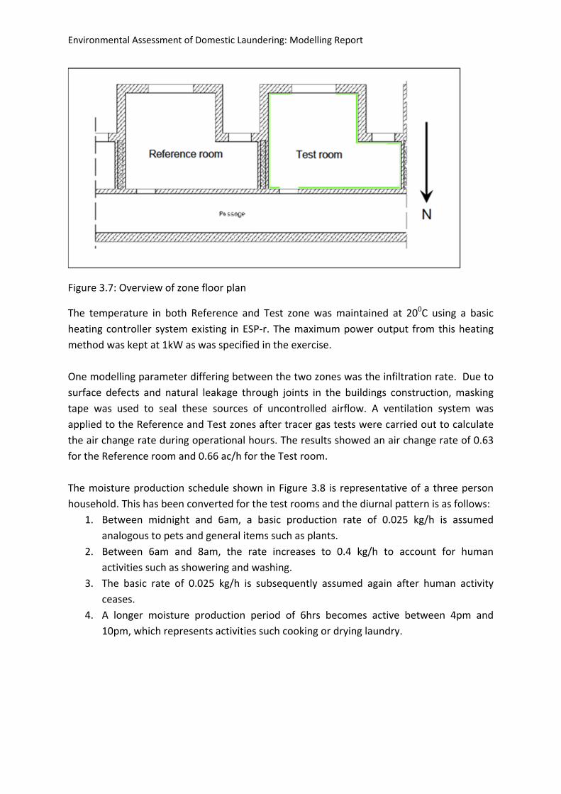
The moisture production schedule shown in Figure 3.8 is representative of a three person
household. This has been converted for the test rooms and the diurnal pattern is as follows:
1. Between midnight and 6am, a basic production rate of 0.025 kg/h is assumed
analogous to pets and general items such as plants.
2. Between 6am and 8am, the rate increases to 0.4 kg/h to account for human
activities such as showering and washing.
3. The basic rate of 0.025 kg/h is subsequently assumed again after human activity
ceases.
4. A longer moisture production period of 6hrs becomes active between 4pm and
10pm, which represents activities such cooking or drying laundry.
Environmental Assessment of Domestic Laundering: Modelling Report
Figure 3.8: Moisture Production schedule
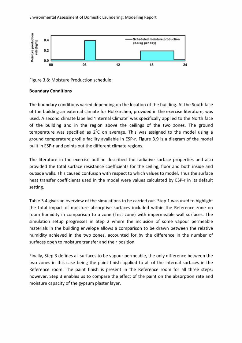
Boundary Conditions
The boundary conditions varied depending on the location of the building. At the South face
of the building an external climate for Holzkirchen, provided in the exercise literature, was
used. A second climate labelled ‘Internal Climate’ was specifically applied to the North face
of the building and in the region above the ceilings of the two zones. The ground
temperature was specified as 20C on average. This was assigned to the model using a
ground temperature profile facility available in ESP‐r. Figure 3.9 is a diagram of the model
built in ESP‐r and points out the different climate regions.
The literature in the exercise outline described the radiative surface properties and also
provided the total surface resistance coefficients for the ceiling, floor and both inside and
outside walls. This caused confusion with respect to which values to model. Thus the surface
heat transfer coefficients used in the model were values calculated by ESP‐r in its default
setting.
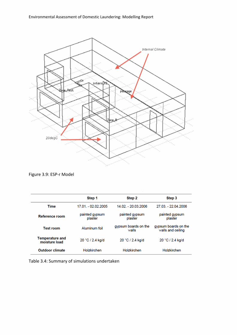
Table 3.4 gives an overview of the simulations to be carried out. Step 1 was used to highlight
the total impact of moisture absorptive surfaces included within the Reference zone on
room humidity in comparison to a zone (Test zone) with impermeable wall surfaces. The
simulation setup progresses in Step 2 where the inclusion of some vapour permeable
materials in the building envelope allows a comparison to be drawn between the relative
humidity achieved in the two zones, accounted for by the difference in the number of
surfaces open to moisture transfer and their position.
Finally, Step 3 defines all surfaces to be vapour permeable, the only difference between the
two zones in this case being the paint finish applied to all of the internal surfaces in the
Reference room. The paint finish is present in the Reference room for all three steps;
however, Step 3 enables us to compare the effect of the paint on the absorption rate and
moisture capacity of the gypsum plaster layer.
Environmental Assessment of Domestic Laundering: Modelling Report
Figure 3.9: ESP‐r Model
Table 3.4: Summary of simulations undertaken
Environmental Assessment of Domestic Laundering: Modelling Report
Results
Step 1
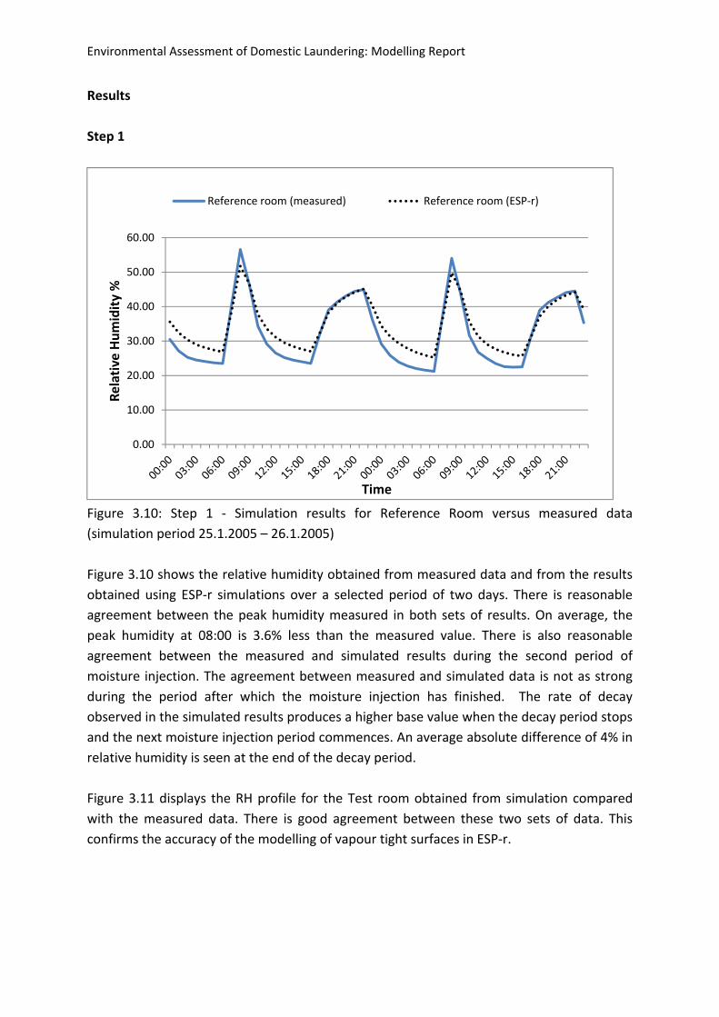
Figure 3.10: Step 1 ‐ Simulation results for Reference Room versus measured data
(simulation period 25.1.2005 – 26.1.2005)
Figure 3.10 shows the relative humidity obtained from measured data and from the results
obtained using ESP‐r simulations over a selected period of two days. There is reasonable
agreement between the peak humidity measured in both sets of results. On average, the
peak humidity at 08:00 is 3.6% less than the measured value. There is also reasonable
agreement between the measured and simulated results during the second period of
moisture injection. The agreement between measured and simulated data is not as strong
during the period after which the moisture injection has finished. The rate of decay
observed in the simulated results produces a higher base value when the decay period stops
and the next moisture injection period commences. An average absolute difference of 4% in
relative humidity is seen at the end of the decay period.
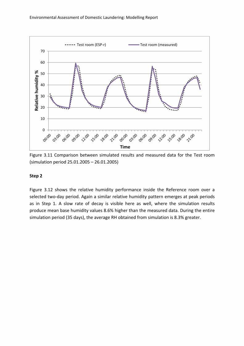
Figure 3.11 displays the RH profile for the Test room obtained from simulation compared
with the measured data. There is good agreement between these two sets of data. This
confirms the accuracy of the modelling of vapour tight surfaces in ESP‐r.
0.00
10.00
20.00
30.00
40.00
50.00
60.00
Relative Humidity %
Time
Reference room (measured) Reference room (ESP‐r)
Environmental Assessment of Domestic Laundering: Modelling Report
Figure 3.11 Comparison between simulated results and measured data for the Test room
(simulation period 25.01.2005 – 26.01.2005)
Step 2
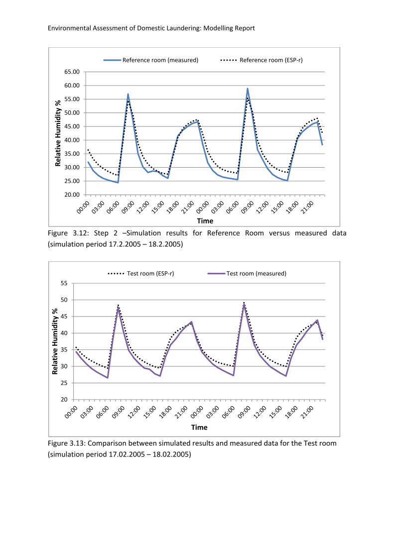
Figure 3.12 shows the relative humidity performance inside the Reference room over a
selected two‐day period. Again a similar relative humidity pattern emerges at peak periods
as in Step 1. A slow rate of decay is visible here as well, where the simulation results
produce mean base humidity values 8.6% higher than the measured data. During the entire
simulation period (35 days), the average RH obtained from simulation is 8.3% greater.
0
10
20
30
40
50
60
70
Relative humidity %
Time
Test room (ESP‐r) Test room (measured)
Environmental Assessment of Domestic Laundering: Modelling Report
Figure 3.12: Step 2 –Simulation results for Reference Room versus measured data
(simulation period 17.2.2005 – 18.2.2005)
Figure 3.13: Comparison between simulated results and measured data for the Test room
(simulation period 17.02.2005 – 18.02.2005)
20.00
25.00
30.00
35.00
40.00
45.00
50.00
55.00
60.00
65.00
Relative Humidity %
Time
Reference room (measured) Reference room (ESP‐r)
20
25
30
35
40
45
50
55
Relative Humidity %
Time
Test room (ESP‐r) Test room (measured)
Environmental Assessment of Domestic Laundering: Modelling Report
Figure 3.13 displays the RH performance in the Test room which changes significantly when
Gypsum Board is applied to the internal wall surfaces. The peak humidity is on average 10%
less than the peak conditions achieved in the Reference room. The buffering potential of the
uncoated Gypsum Board is clearly more effective than the coated plaster. The higher
infiltration rate in the Test room, however, does not remove the emitted moisture
sufficiently to match the base RH value that is achieved in the Reference room.
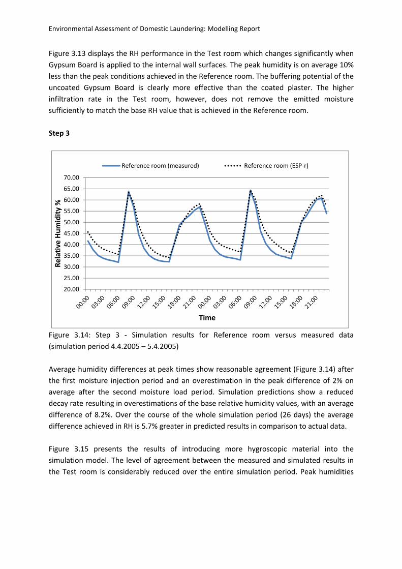
Step 3
Figure 3.14: Step 3 ‐ Simulation results for Reference room versus measured data
(simulation period 4.4.2005 – 5.4.2005)
Average humidity differences at peak times show reasonable agreement (Figure 3.14) after
the first moisture injection period and an overestimation in the peak difference of 2% on
average after the second moisture load period. Simulation predictions show a reduced
decay rate resulting in overestimations of the base relative humidity values, with an average
difference of 8.2%. Over the course of the whole simulation period (26 days) the average
difference achieved in RH is 5.7% greater in predicted results in comparison to actual data.
Figure 3.15 presents the results of introducing more hygroscopic material into the
simulation model. The level of agreement between the measured and simulated results in
the Test room is considerably reduced over the entire simulation period. Peak humidities
20.00
25.00
30.00
35.00
40.00
45.00
50.00
55.00
60.00
65.00
70.00
Relative Humidity %
Time
Reference room (measured) Reference room (ESP‐r)
Environmental Assessment of Domestic Laundering: Modelling Report
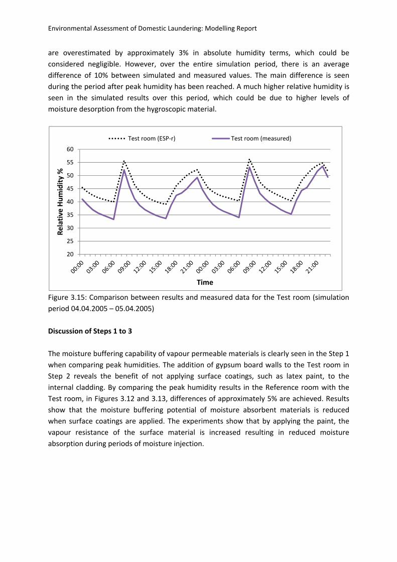
are overestimated by approximately 3% in absolute humidity terms, which could be
considered negligible. However, over the entire simulation period, there is an average
difference of 10% between simulated and measured values. The main difference is seen
during the period after peak humidity has been reached. A much higher relative humidity is
seen in the simulated results over this period, which could be due to higher levels of
moisture desorption from the hygroscopic material.
Figure 3.15: Comparison between results and measured data for the Test room (simulation
period 04.04.2005 – 05.04.2005)
Discussion of Steps 1 to 3
The moisture buffering capability of vapour permeable materials is clearly seen in the Step 1
when comparing peak humidities. The addition of gypsum board walls to the Test room in
Step 2 reveals the benefit of not applying surface coatings, such as latex paint, to the
internal cladding. By comparing the peak humidity results in the Reference room with the
Test room, in Figures 3.12 and 3.13, differences of approximately 5% are achieved. Results
show that the moisture buffering potential of moisture absorbent materials is reduced
when surface coatings are applied. The experiments show that by applying the paint, the
vapour resistance of the surface material is increased resulting in reduced moisture
absorption during periods of moisture injection.
20
25
30
35
40
45
50
55
60
Relative Humidity %
Time
Test room (ESP‐r) Test room (measured)

Environmental Assessment of Domestic Laundering: Modelling Report
From Step 3, it can be seen that the uncoated Gypsum Board at the internal surfaces is more
effective than Gypsum Plaster coated with latex paint at helping to reduce relative humidity
peaks. Reduced fluctuations in the relative humidity are also achieved by applying the
uncoated Gypsum Board. Smaller RH fluctuations in the air will ultimately be beneficial for
the long‐term integrity and durability of the construction material. By repeatedly exposing
the material to long periods of high moisture loads, 70% and above, the possibility of
surface degradation through biological corrosion increases and in addition the onset of
health related problems for occupants begins as a result of mould growth.
3.2 Cyclic tests
See note at the end of the report contents.
Environmental Assessment of Domestic Laundering: Modelling Report
4. Modelling ‐ General Parametric Study
An initial parametric study was undertaken to assess the impact of a range of parameters on
indoor relative humidity and energy consumption. These included moisture production
levels, ventilation rates, surface finishes, insulation levels, levels and climate. The
parametric values chosen were to cover the likely maximum realistic range for the
investigated parameters
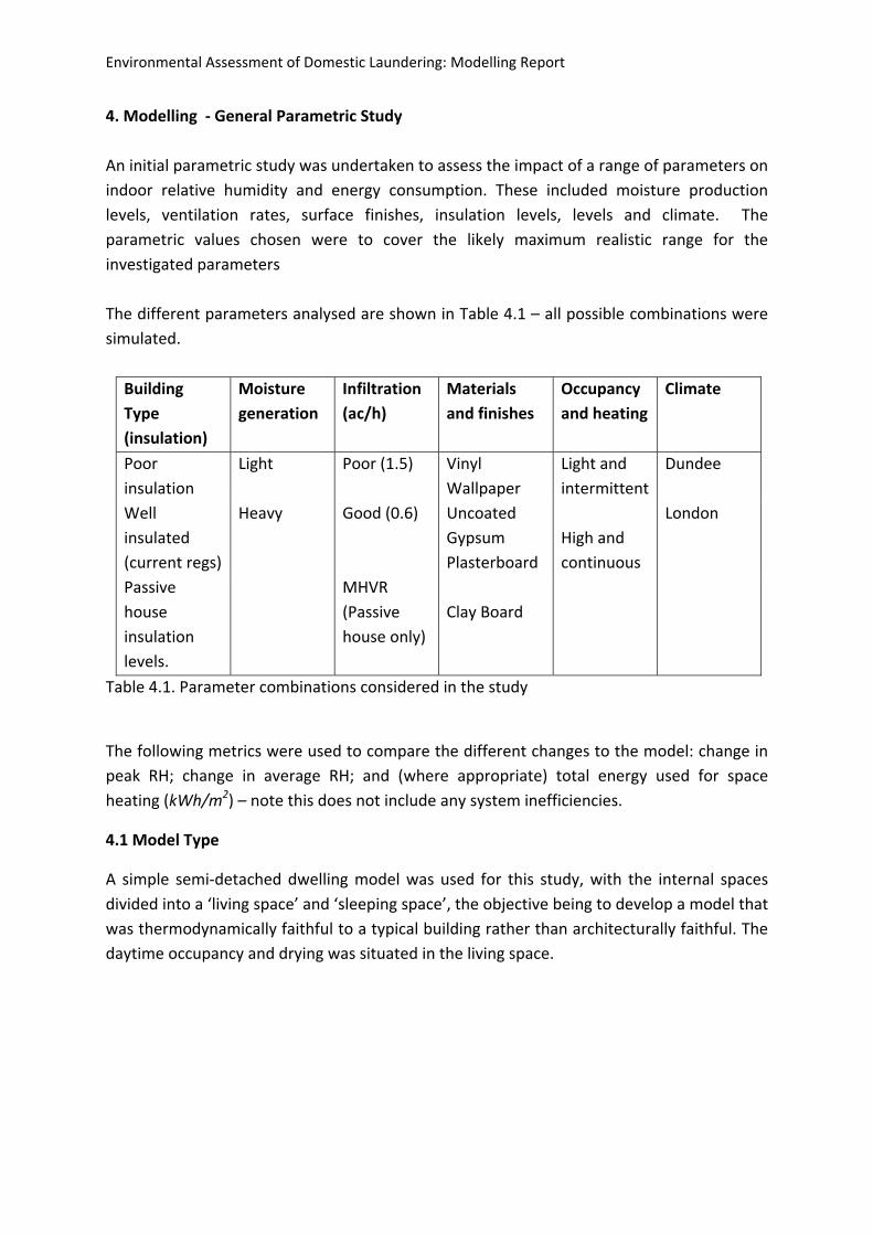
The different parameters analysed are shown in Table 4.1 – all possible combinations were
simulated.
Building
Type
(insulation)
Moisture
generation
Infiltration
(ac/h)
Materials
and finishes
Occupancy
and heating
Climate
Poor
insulation
Light Poor (1.5) Vinyl
Wallpaper
Light and
intermittent
Dundee
Well
insulated
(current regs)
Heavy Good (0.6) Uncoated
Gypsum
Plasterboard
High and
continuous
London
Passive
house
insulation
levels.
MHVR
(Passive
house only)
Clay Board
Table 4.1. Parameter combinations considered in the study
The following metrics were used to compare the different changes to the model: change in
peak RH; change in average RH; and (where appropriate) total energy used for space
heating (kWh/m2) – note this does not include any system inefficiencies.
4.1 Model Type
A simple semi‐detached dwelling model was used for this study, with the internal spaces
divided into a ‘living space’ and ‘sleeping space’, the objective being to develop a model that
was thermodynamically faithful to a typical building rather than architecturally faithful. The
daytime occupancy and drying was situated in the living space.
Environmental Assessment of Domestic Laundering: Modelling Report
ESP‐r models and Passive House Insulation Levels
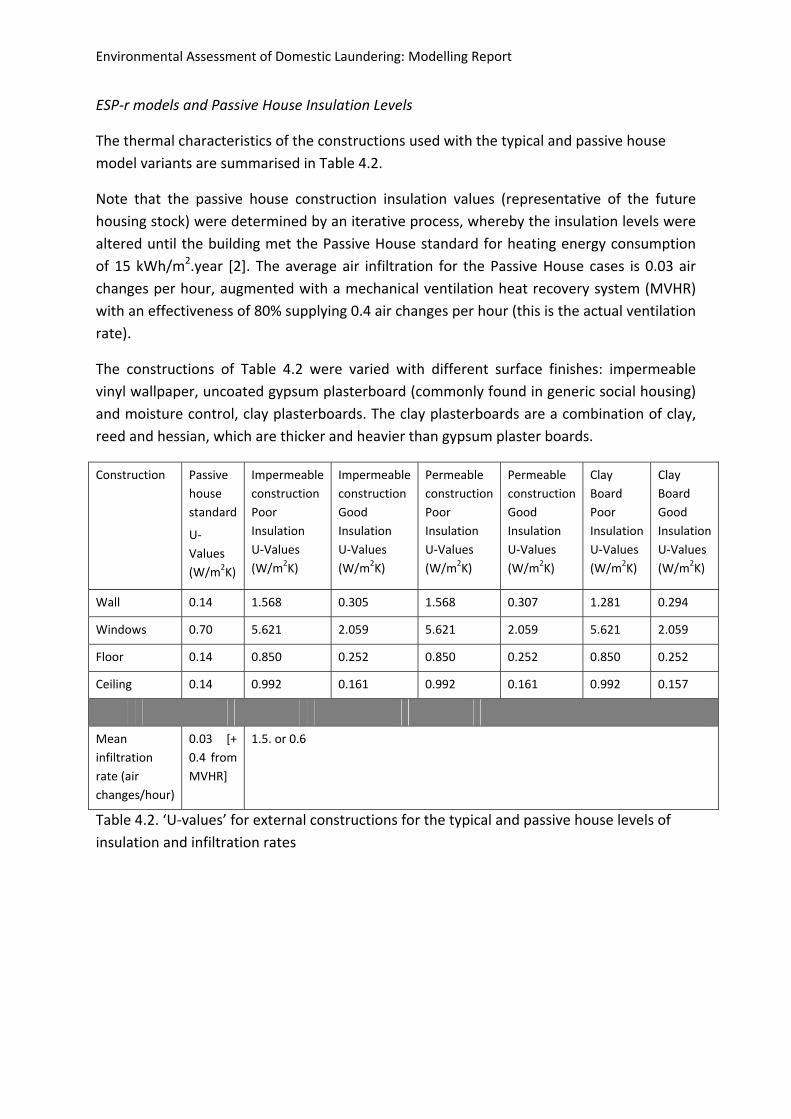
The thermal characteristics of the constructions used with the typical and passive house
model variants are summarised in Table 4.2.
Note that the passive house construction insulation values (representative of the future
housing stock) were determined by an iterative process, whereby the insulation levels were
altered until the building met the Passive House standard for heating energy consumption
of 15 kWh/m2.year [2]. The average air infiltration for the Passive House cases is 0.03 air
changes per hour, augmented with a mechanical ventilation heat recovery system (MVHR)
with an effectiveness of 80% supplying 0.4 air changes per hour (this is the actual ventilation
rate).
The constructions of Table 4.2 were varied with different surface finishes: impermeable
vinyl wallpaper, uncoated gypsum plasterboard (commonly found in generic social housing)
and moisture control, clay plasterboards. The clay plasterboards are a combination of clay,
reed and hessian, which are thicker and heavier than gypsum plaster boards.
Construction Passive
house
standard
U‐
Values
(W/m2K)
Impermeable
construction
Poor
Insulation
U‐Values
(W/m2K)
Impermeable
construction
Good
Insulation
U‐Values
(W/m2K)
Permeable
construction
Poor
Insulation
U‐Values
(W/m2K)
Permeable
construction
Good
Insulation
U‐Values
(W/m2K)
Clay
Board
Poor
Insulation
U‐Values
(W/m2K)
Clay
Board
Good
Insulation
U‐Values
(W/m2K)
Wall 0.14 1.568 0.305 1.568 0.307 1.281 0.294
Windows 0.70 5.621 2.059 5.621 2.059 5.621 2.059
Floor 0.14 0.850 0.252 0.850 0.252 0.850 0.252
Ceiling 0.14 0.992 0.161 0.992 0.161 0.992 0.157
Mean
infiltration
rate (air
changes/hour)
0.03 [+
0.4 from
MVHR]
1.5. or 0.6
Table 4.2. ‘U‐values’ for external constructions for the typical and passive house levels of
insulation and infiltration rates
Environmental Assessment of Domestic Laundering: Modelling Report
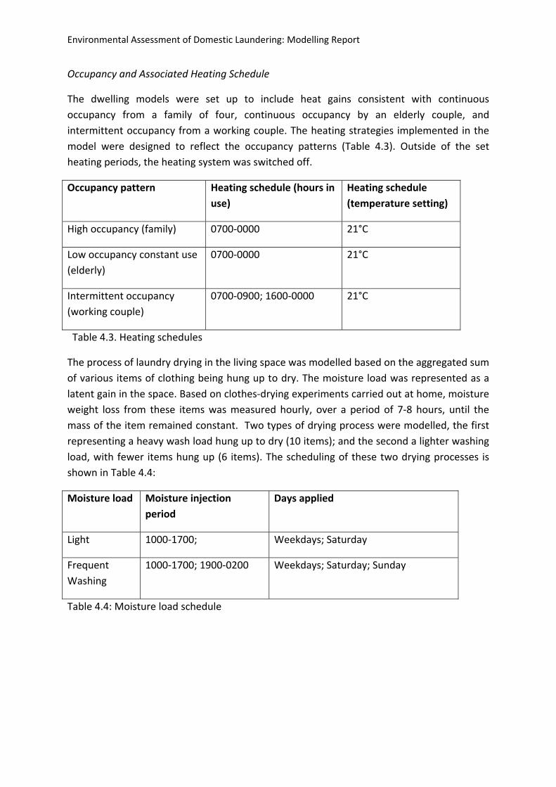
Occupancy and Associated Heating Schedule
The dwelling models were set up to include heat gains consistent with continuous
occupancy from a family of four, continuous occupancy by an elderly couple, and
intermittent occupancy from a working couple. The heating strategies implemented in the
model were designed to reflect the occupancy patterns (Table 4.3). Outside of the set
heating periods, the heating system was switched off.
Occupancy pattern Heating schedule (hours in
use)
Heating schedule
(temperature setting)
High occupancy (family) 0700‐0000 21°C
Low occupancy constant use
(elderly)
0700‐0000 21°C
Intermittent occupancy
(working couple)
0700‐0900; 1600‐0000 21°C
Table 4.3. Heating schedules
The process of laundry drying in the living space was modelled based on the aggregated sum
of various items of clothing being hung up to dry. The moisture load was represented as a
latent gain in the space. Based on clothes‐drying experiments carried out at home, moisture
weight loss from these items was measured hourly, over a period of 7‐8 hours, until the
mass of the item remained constant. Two types of drying process were modelled, the first
representing a heavy wash load hung up to dry (10 items); and the second a lighter washing
load, with fewer items hung up (6 items). The scheduling of these two drying processes is
shown in Table 4.4:
Moisture load Moisture injection
period
Days applied
Light 1000‐1700; Weekdays; Saturday
Frequent
Washing
1000‐1700; 1900‐0200 Weekdays; Saturday; Sunday
Table 4.4: Moisture load schedule
Environmental Assessment of Domestic Laundering: Modelling Report
Infiltration Rates
A range of air change rates were investigated. For these simulations, an air change rate of
0.6 was used for a ‘tight’ construction and a rate of 1.5 was used to represent a more leaky
construction characteristic of older dwellings.
4.2 Parametric Study Results
Figures 4.1 and 4.2 are indicative of the results emerging from the parametric study and
show the extreme ranges of mean RH, maximum RH and energy from the different
simulations for specific parametric changes to the models as outlined in Table 4.1. The
maximum values on these graphs show the maximum potential impact of the tested
parameters on the living room RH. For example, the greatest difference in mean RH (in
summer and winter) due to changing the surface materials was about 15% between all
parametric variations tested. The figures illustrate the relative importance of material
finishes on the RH, indicating that (particularly in summer) changing internal material
finishes can result in changes to RH of a comparable magnitude as changes caused by
variations in both moisture load and infiltration. However both moisture loading and
ventilation levels had a more significant effect on the mean RH.
Figure 4.1: absolute change in RH (%) for winter simulations
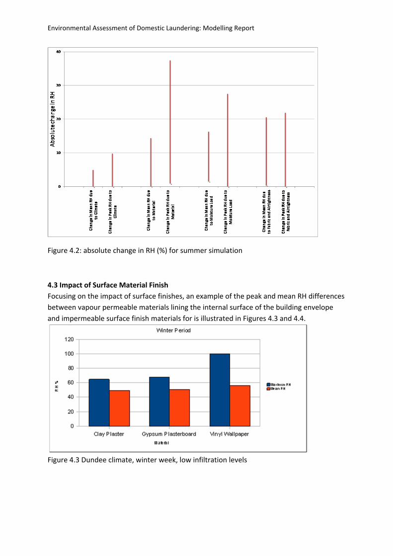
Environmental Assessment of Domestic Laundering: Modelling Report
Figure 4.2: absolute change in RH (%) for summer simulation
4.3 Impact of Surface Material Finish
Focusing on the impact of surface finishes, an example of the peak and mean RH differences
between vapour permeable materials lining the internal surface of the building envelope
and impermeable surface finish materials for is illustrated in Figures 4.3 and 4.4.
Figure 4.3 Dundee climate, winter week, low infiltration levels
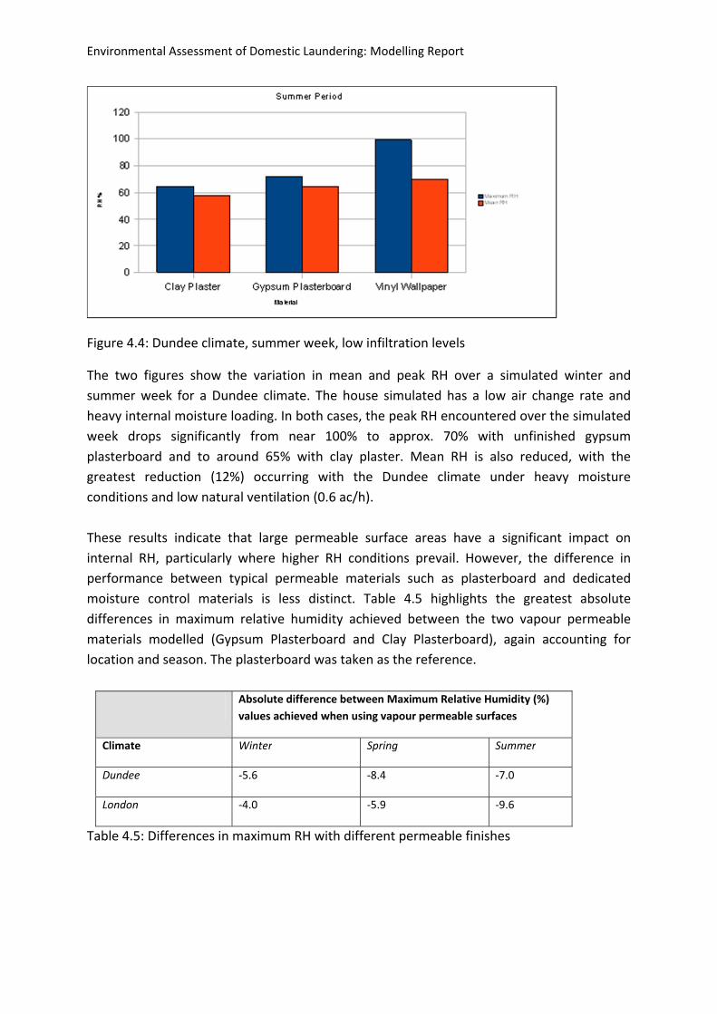
Environmental Assessment of Domestic Laundering: Modelling Report
Figure 4.4: Dundee climate, summer week, low infiltration levels
The two figures show the variation in mean and peak RH over a simulated winter and
summer week for a Dundee climate. The house simulated has a low air change rate and
heavy internal moisture loading. In both cases, the peak RH encountered over the simulated
week drops significantly from near 100% to approx. 70% with unfinished gypsum
plasterboard and to around 65% with clay plaster. Mean RH is also reduced, with the
greatest reduction (12%) occurring with the Dundee climate under heavy moisture
conditions and low natural ventilation (0.6 ac/h).
These results indicate that large permeable surface areas have a significant impact on
internal RH, particularly where higher RH conditions prevail. However, the difference in
performance between typical permeable materials such as plasterboard and dedicated
moisture control materials is less distinct. Table 4.5 highlights the greatest absolute
differences in maximum relative humidity achieved between the two vapour permeable
materials modelled (Gypsum Plasterboard and Clay Plasterboard), again accounting for
location and season. The plasterboard was taken as the reference.
Absolute difference between Maximum Relative Humidity (%)
values achieved when using vapour permeable surfaces
Climate Winter Spring Summer
Dundee ‐5.6 ‐8.4 ‐7.0
London ‐4.0 ‐5.9 ‐9.6
Table 4.5: Differences in maximum RH with different permeable finishes
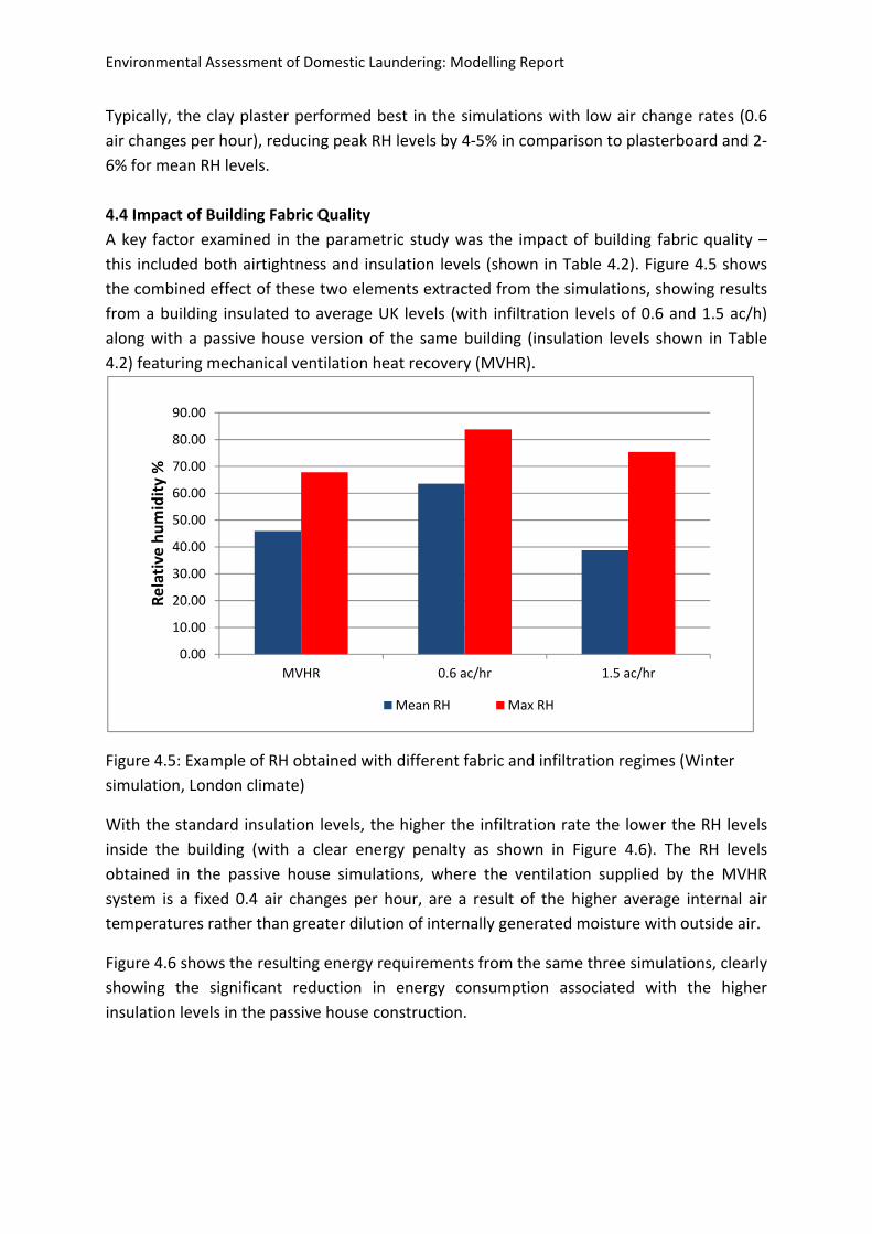
Environmental Assessment of Domestic Laundering: Modelling Report
Typically, the clay plaster performed best in the simulations with low air change rates (0.6
air changes per hour), reducing peak RH levels by 4‐5% in comparison to plasterboard and 2‐
6% for mean RH levels.
4.4 Impact of Building Fabric Quality
A key factor examined in the parametric study was the impact of building fabric quality –
this included both airtightness and insulation levels (shown in Table 4.2). Figure 4.5 shows
the combined effect of these two elements extracted from the simulations, showing results
from a building insulated to average UK levels (with infiltration levels of 0.6 and 1.5 ac/h)
along with a passive house version of the same building (insulation levels shown in Table
4.2) featuring mechanical ventilation heat recovery (MVHR).
Figure 4.5: Example of RH obtained with different fabric and infiltration regimes (Winter
simulation, London climate)
With the standard insulation levels, the higher the infiltration rate the lower the RH levels
inside the building (with a clear energy penalty as shown in Figure 4.6). The RH levels
obtained in the passive house simulations, where the ventilation supplied by the MVHR
system is a fixed 0.4 air changes per hour, are a result of the higher average internal air
temperatures rather than greater dilution of internally generated moisture with outside air.
Figure 4.6 shows the resulting energy requirements from the same three simulations, clearly
showing the significant reduction in energy consumption associated with the higher
insulation levels in the passive house construction.
0.00
10.00
20.00
30.00
40.00
50.00
60.00
70.00
80.00
90.00
MVHR 0.6 ac/hr 1.5 ac/hr
Relative humidity %
Mean RH Max RH
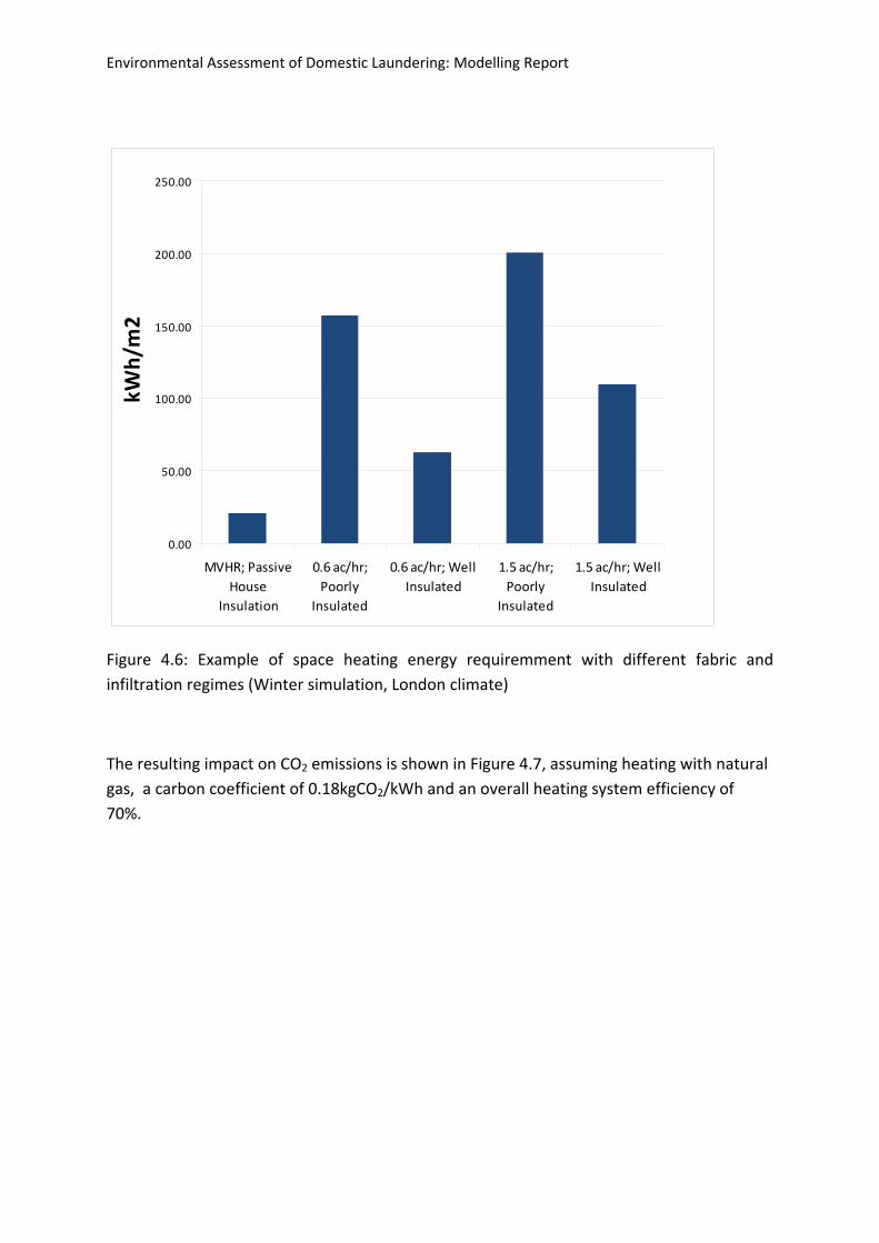
Environmental Assessment of Domestic Laundering: Modelling Report
Figure 4.6: Example of space heating energy requiremment with different fabric and
infiltration regimes (Winter simulation, London climate)
The resulting impact on CO2 emissions is shown in Figure 4.7, assuming heating with natural
gas, a carbon coefficient of 0.18kgCO2/kWh and an overall heating system efficiency of
70%.
kWh/m
2
0.00
50.00
100.00
150.00
200.00
250.00
MVHR; Passive
House
Insulation
0.6 ac/hr;
Poorly
Insulated
0.6 ac/hr; Well
Insulated
1.5 ac/hr;
Poorly
Insulated
1.5 ac/hr; Well
Insulated
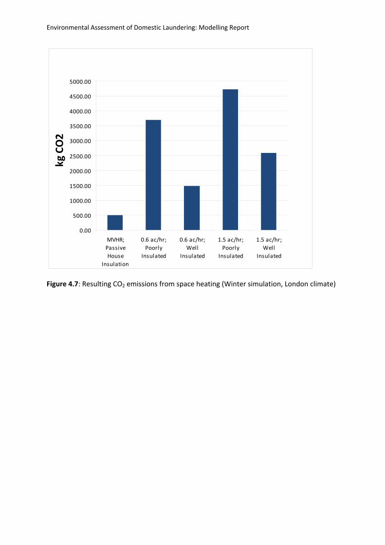
Environmental Assessment of Domestic Laundering: Modelling Report
Figure 4.7: Resulting CO2 emissions from space heating (Winter simulation, London climate)
kg CO2
0.00
500.00
1000.00
1500.00
2000.00
2500.00
3000.00
3500.00
4000.00
4500.00
5000.00
MVHR;
Passive
House
Insulation
0.6 ac/hr;
Poorly
Insulated
0.6 ac/hr;
Well
Insulated
1.5 ac/hr;
Poorly
Insulated
1.5 ac/hr;
Well
Insulated
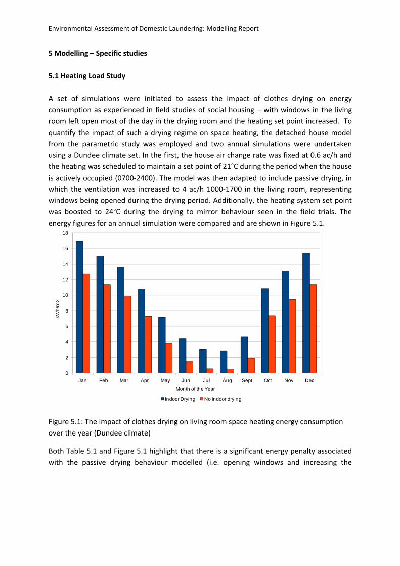
Environmental Assessment of Domestic Laundering: Modelling Report
5 Modelling – Specific studies
5.1 Heating Load Study
A set of simulations were initiated to assess the impact of clothes drying on energy
consumption as experienced in field studies of social housing – with windows in the living
room left open most of the day in the drying room and the heating set point increased. To
quantify the impact of such a drying regime on space heating, the detached house model
from the parametric study was employed and two annual simulations were undertaken
using a Dundee climate set. In the first, the house air change rate was fixed at 0.6 ac/h and
the heating was scheduled to maintain a set point of 21°C during the period when the house
is actively occupied (0700‐2400). The model was then adapted to include passive drying, in
which the ventilation was increased to 4 ac/h 1000‐1700 in the living room, representing
windows being opened during the drying period. Additionally, the heating system set point
was boosted to 24°C during the drying to mirror behaviour seen in the field trials. The
energy figures for an annual simulation were compared and are shown in Figure 5.1.
Figure 5.1: The impact of clothes drying on living room space heating energy consumption
over the year (Dundee climate)
Both Table 5.1 and Figure 5.1 highlight that there is a significant energy penalty associated
with the passive drying behaviour modelled (i.e. opening windows and increasing the
0
2
4
6
8
10
12
14
16
18
Jan Feb Mar Apr May Jun Jul Aug Sept Oct Nov Dec
kWh
/m2
Month of the Year
Indoor Drying No Indoor drying
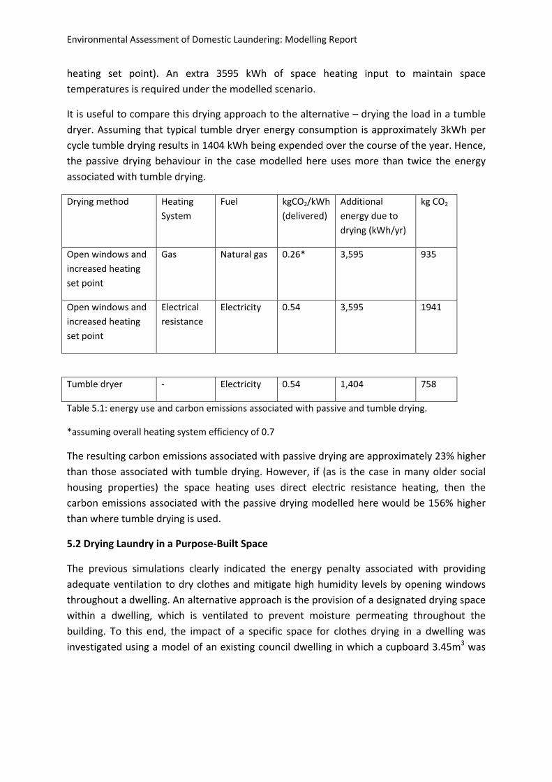
Environmental Assessment of Domestic Laundering: Modelling Report
heating set point). An extra 3595 kWh of space heating input to maintain space
temperatures is required under the modelled scenario.
It is useful to compare this drying approach to the alternative – drying the load in a tumble
dryer. Assuming that typical tumble dryer energy consumption is approximately 3kWh per
cycle tumble drying results in 1404 kWh being expended over the course of the year. Hence,
the passive drying behaviour in the case modelled here uses more than twice the energy
associated with tumble drying.
Drying method Heating
System
Fuel kgCO2/kWh
(delivered)
Additional
energy due to
drying (kWh/yr)
kg CO2
Open windows and
increased heating
set point
Gas Natural gas 0.26* 3,595 935
Open windows and
increased heating
set point
Electrical
resistance
Electricity 0.54 3,595 1941
Tumble dryer ‐ Electricity 0.54 1,404 758
Table 5.1: energy use and carbon emissions associated with passive and tumble drying.
*assuming overall heating system efficiency of 0.7
The resulting carbon emissions associated with passive drying are approximately 23% higher
than those associated with tumble drying. However, if (as is the case in many older social
housing properties) the space heating uses direct electric resistance heating, then the
carbon emissions associated with the passive drying modelled here would be 156% higher
than where tumble drying is used.
5.2 Drying Laundry in a Purpose‐Built Space
The previous simulations clearly indicated the energy penalty associated with providing
adequate ventilation to dry clothes and mitigate high humidity levels by opening windows
throughout a dwelling. An alternative approach is the provision of a designated drying space
within a dwelling, which is ventilated to prevent moisture permeating throughout the
building. To this end, the impact of a specific space for clothes drying in a dwelling was
investigated using a model of an existing council dwelling in which a cupboard 3.45m3 was
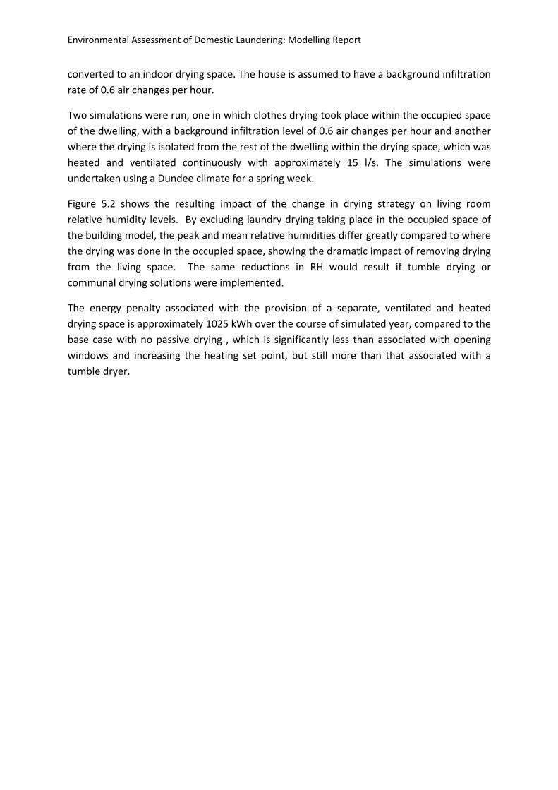
Environmental Assessment of Domestic Laundering: Modelling Report
converted to an indoor drying space. The house is assumed to have a background infiltration
rate of 0.6 air changes per hour.
Two simulations were run, one in which clothes drying took place within the occupied space
of the dwelling, with a background infiltration level of 0.6 air changes per hour and another
where the drying is isolated from the rest of the dwelling within the drying space, which was
heated and ventilated continuously with approximately 15 l/s. The simulations were
undertaken using a Dundee climate for a spring week.
Figure 5.2 shows the resulting impact of the change in drying strategy on living room
relative humidity levels. By excluding laundry drying taking place in the occupied space of
the building model, the peak and mean relative humidities differ greatly compared to where
the drying was done in the occupied space, showing the dramatic impact of removing drying
from the living space. The same reductions in RH would result if tumble drying or
communal drying solutions were implemented.
The energy penalty associated with the provision of a separate, ventilated and heated
drying space is approximately 1025 kWh over the course of simulated year, compared to the
base case with no passive drying , which is significantly less than associated with opening
windows and increasing the heating set point, but still more than that associated with a
tumble dryer.
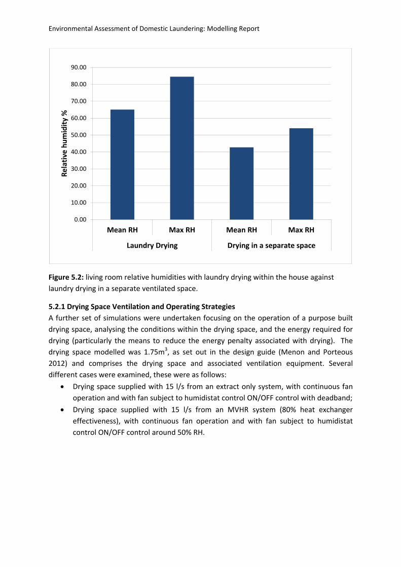
Environmental Assessment of Domestic Laundering: Modelling Report
Figure 5.2: living room relative humidities with laundry drying within the house against
laundry drying in a separate ventilated space.
5.2.1 Drying Space Ventilation and Operating Strategies
A further set of simulations were undertaken focusing on the operation of a purpose built
drying space, analysing the conditions within the drying space, and the energy required for
drying (particularly the means to reduce the energy penalty associated with drying). The
drying space modelled was 1.75m3, as set out in the design guide (Menon and Porteous
2012) and comprises the drying space and associated ventilation equipment. Several
different cases were examined, these were as follows:
Drying space supplied with 15 l/s from an extract only system, with continuous fan
operation and with fan subject to humidistat control ON/OFF control with deadband;
Drying space supplied with 15 l/s from an MVHR system (80% heat exchanger
effectiveness), with continuous fan operation and with fan subject to humidistat
control ON/OFF control around 50% RH.
0.00
10.00
20.00
30.00
40.00
50.00
60.00
70.00
80.00
90.00
Mean RH Max RH Mean RH Max RH
Laundry Drying Drying in a separate space
Relative humidity %
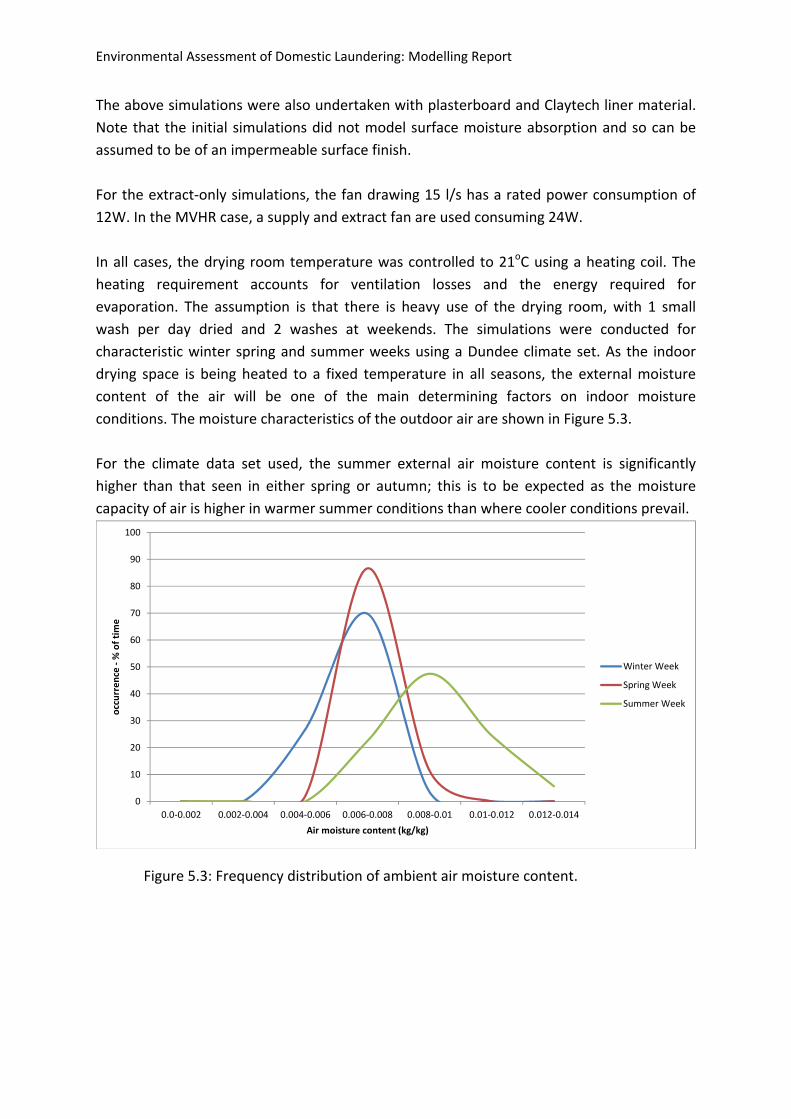
Environmental Assessment of Domestic Laundering: Modelling Report
The above simulations were also undertaken with plasterboard and Claytech liner material.
Note that the initial simulations did not model surface moisture absorption and so can be
assumed to be of an impermeable surface finish.
For the extract‐only simulations, the fan drawing 15 l/s has a rated power consumption of
12W. In the MVHR case, a supply and extract fan are used consuming 24W.
In all cases, the drying room temperature was controlled to 21oC using a heating coil. The
heating requirement accounts for ventilation losses and the energy required for
evaporation. The assumption is that there is heavy use of the drying room, with 1 small
wash per day dried and 2 washes at weekends. The simulations were conducted for
characteristic winter spring and summer weeks using a Dundee climate set. As the indoor
drying space is being heated to a fixed temperature in all seasons, the external moisture
content of the air will be one of the main determining factors on indoor moisture
conditions. The moisture characteristics of the outdoor air are shown in Figure 5.3.
For the climate data set used, the summer external air moisture content is significantly
higher than that seen in either spring or autumn; this is to be expected as the moisture
capacity of air is higher in warmer summer conditions than where cooler conditions prevail.
Figure 5.3: Frequency distribution of ambient air moisture content.
0
10
20
30
40
50
60
70
80
90
100
0.0‐0.002 0.002‐0.004 0.004‐0.006 0.006‐0.008 0.008‐0.01 0.01‐0.012 0.012‐0.014
occurrence ‐% of time
Air moisture content (kg/kg)
Winter Week
Spring Week
Summer Week
Environmental Assessment of Domestic Laundering: Modelling Report
CASE 1 – Impermeable Finish, Extract Only (no heat recovery)
Figure 5.4 shows the typical time‐series output from one of the spring simulations with the
fan supplying the drying space operating continuously at 15 l/s. Points to note are that the
drying activity raises the RH by approximately 25% and drops the space temperature by
around 3oC before they recover due to the action of space heating control, which tries to
maintain the temperature at 21oC. Also notice that whilst external RH is high, when this air
is brought into the drying space and heated, the internal RH is maintained around 30%
outwith the drying period.
Figure 5.4. Typical results a simulation – spring, continuous fan operation, extract only.
Figure 5.5 and Table 5.2 summarise the time‐series results from 6 simulations for the case
with the fan running continuously at 15 l/s and where the fan runs only to limit humidity
levels, using an on/off controller with a dead band of 50‐70% RH, for winter spring and
summer weeks. The results comprise the mean temperature, mean RH, peak RH and energy
use for the fan and heater (kWh).
0
5
10
15
20
25
0
10
20
30
40
50
60
70
80
90
100
0 2000 4000 6000 8000 10000
Temperature (degC)
RH %
Time (mins)
Drying room RH Spring RH Drying room temp
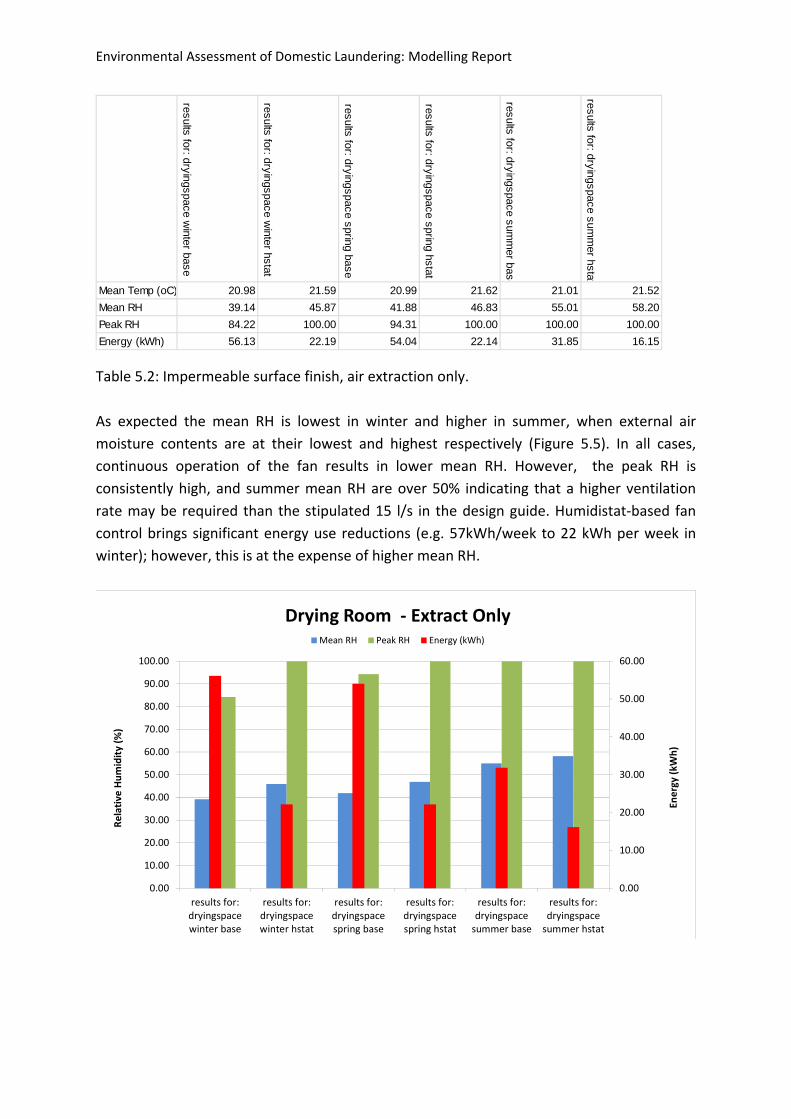
Environmental Assessment of Domestic Laundering: Modelling Report
Table 5.2: Impermeable surface finish, air extraction only.
As expected the mean RH is lowest in winter and higher in summer, when external air
moisture contents are at their lowest and highest respectively (Figure 5.5). In all cases,
continuous operation of the fan results in lower mean RH. However, the peak RH is
consistently high, and summer mean RH are over 50% indicating that a higher ventilation
rate may be required than the stipulated 15 l/s in the design guide. Humidistat‐based fan
control brings significant energy use reductions (e.g. 57kWh/week to 22 kWh per week in
winter); however, this is at the expense of higher mean RH.
results for: dryingspace winter base
results for: dryingspace winter hstat
results for: dryingspace spring base
results for: dryingspace spring hstat
results for: dryingspace summ
er base
results for: dryingspace summ
er hstat
Mean Temp (oC) 20.98 21.59 20.99 21.62 21.01 21.52
Mean RH 39.14 45.87 41.88 46.83 55.01 58.20
Peak RH 84.22 100.00 94.31 100.00 100.00 100.00
Energy (kWh) 56.13 22.19 54.04 22.14 31.85 16.15
0.00
10.00
20.00
30.00
40.00
50.00
60.00
0.00
10.00
20.00
30.00
40.00
50.00
60.00
70.00
80.00
90.00
100.00
results for:dryingspacewinter base
results for:dryingspacewinter hstat
results for:dryingspacespring base
results for:dryingspacespring hstat
results for:dryingspacesummer base
results for:dryingspacesummer hstat
Energy (kWh)
Relative
Humidity (%
)
Drying Room ‐ Extract OnlyMean RH Peak RH Energy (kWh)
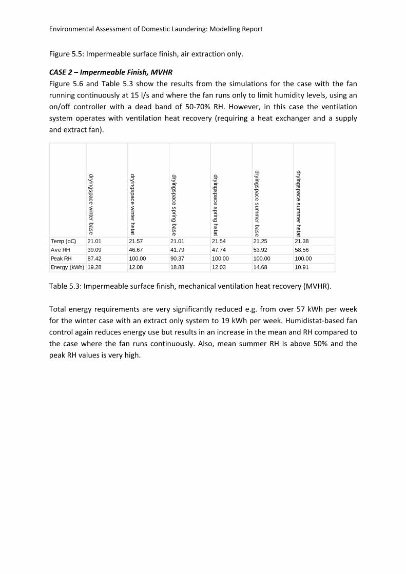
Environmental Assessment of Domestic Laundering: Modelling Report
Figure 5.5: Impermeable surface finish, air extraction only.
CASE 2 – Impermeable Finish, MVHR
Figure 5.6 and Table 5.3 show the results from the simulations for the case with the fan
running continuously at 15 l/s and where the fan runs only to limit humidity levels, using an
on/off controller with a dead band of 50‐70% RH. However, in this case the ventilation
system operates with ventilation heat recovery (requiring a heat exchanger and a supply
and extract fan).
Table 5.3: Impermeable surface finish, mechanical ventilation heat recovery (MVHR).
Total energy requirements are very significantly reduced e.g. from over 57 kWh per week
for the winter case with an extract only system to 19 kWh per week. Humidistat‐based fan
control again reduces energy use but results in an increase in the mean and RH compared to
the case where the fan runs continuously. Also, mean summer RH is above 50% and the
peak RH values is very high.
dryingspace winter base
dryingspace winter hstat
dryingspace spring base
dryingspace spring hstat
dryingspace summ
er base
dryingspace summ
er hstat
Temp (oC) 21.01 21.57 21.01 21.54 21.25 21.38
Ave RH 39.09 46.67 41.79 47.74 53.92 58.56
Peak RH 87.42 100.00 90.37 100.00 100.00 100.00
Energy (kWh) 19.28 12.08 18.88 12.03 14.68 10.91
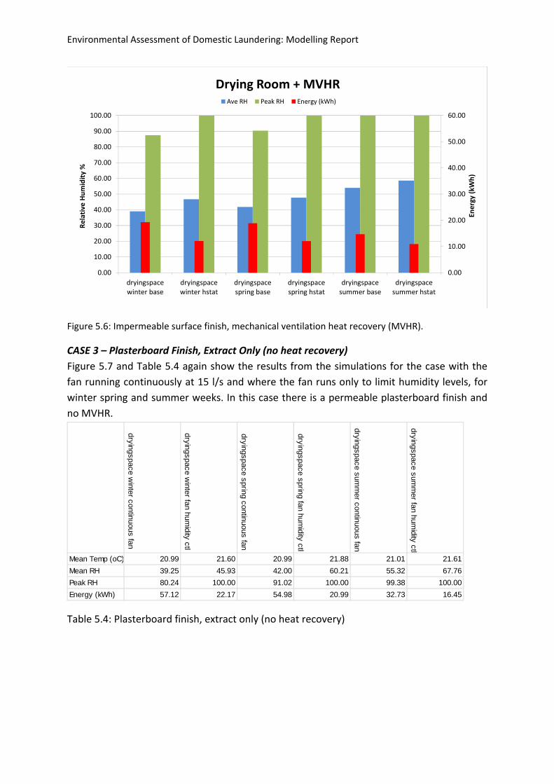
Environmental Assessment of Domestic Laundering: Modelling Report
Figure 5.6: Impermeable surface finish, mechanical ventilation heat recovery (MVHR).
CASE 3 – Plasterboard Finish, Extract Only (no heat recovery)
Figure 5.7 and Table 5.4 again show the results from the simulations for the case with the
fan running continuously at 15 l/s and where the fan runs only to limit humidity levels, for
winter spring and summer weeks. In this case there is a permeable plasterboard finish and
no MVHR.
Table 5.4: Plasterboard finish, extract only (no heat recovery)
0.00
10.00
20.00
30.00
40.00
50.00
60.00
0.00
10.00
20.00
30.00
40.00
50.00
60.00
70.00
80.00
90.00
100.00
dryingspacewinter base
dryingspacewinter hstat
dryingspacespring base
dryingspacespring hstat
dryingspacesummer base
dryingspacesummer hstat
Energy (kWh)
Relative
Humidity %
Drying Room + MVHRAve RH Peak RH Energy (kWh)
dryingspace winter continuous fan
dryingspace winter fan hum
idity ctl
dryingspace spring continuous fan
dryingspace spring fan humidity ctl
dryingspace summ
er continuous fan
dryingspace summ
er fan humidity ctl
Mean Temp (oC) 20.99 21.60 20.99 21.88 21.01 21.61
Mean RH 39.25 45.93 42.00 60.21 55.32 67.76
Peak RH 80.24 100.00 91.02 100.00 99.38 100.00
Energy (kWh) 57.12 22.17 54.98 20.99 32.73 16.45
Environmental Assessment of Domestic Laundering: Modelling Report
The results indicate that changing the surface finish has a marginal effect on energy
consumption. Mean RH increases in spring and summer when the fan is subject to humidity
control in comparison to the impermeable case there is a very slight reduction in some peak
RH. Humidistat‐based fan control has a significant beneficial effect on energy consumption,
at the expense of poorer control of RH.
Figure 5.7: Plasterboard finish, extract only (no heat recovery)
CASE 4 – Plasterboard Finish, MVHR
Figure 5.8 and Table 5.5 show the results from the simulations for the case with the fans
running continuously at 15 l/s and where the fan runs only to limit humidity levels, using an
on/off controller with a dead band of 50‐70% RH. In this case the ventilation system is
configured for MVHR with a heat exchanger and a supply and extract fan.
0.00
10.00
20.00
30.00
40.00
50.00
60.00
0.00
10.00
20.00
30.00
40.00
50.00
60.00
70.00
80.00
90.00
100.00
dryingspacewinter
continuous fan
dryingspacewinter fanhumidity ctl
dryingspacespring continuous
fan
dryingspacespring fanhumidity ctl
dryingspacesummer
continuous fan
dryingspacesummer fanhumidity ctl
Energy (kWh)
Relative Humidity (%
)
Drying Room ‐ Extract OnlyMean RH Peak RH Energy (kWh)
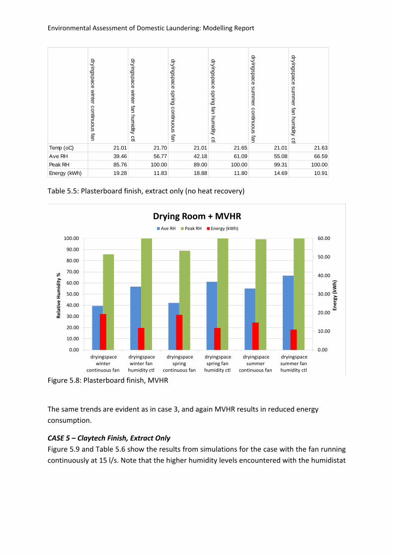
Environmental Assessment of Domestic Laundering: Modelling Report
Table 5.5: Plasterboard finish, extract only (no heat recovery)
Figure 5.8: Plasterboard finish, MVHR
The same trends are evident as in case 3, and again MVHR results in reduced energy
consumption.
CASE 5 – Claytech Finish, Extract Only
Figure 5.9 and Table 5.6 show the results from simulations for the case with the fan running
continuously at 15 l/s. Note that the higher humidity levels encountered with the humidistat
dryingspace winter continuous fan
dryingspace winter fan hum
idity ctl
dryingspace spring continuous fan
dryingspace spring fan humidity ctl
dryingspace summ
er continuous fan
dryingspace summ
er fan humidity ctl
Temp (oC) 21.01 21.70 21.01 21.65 21.01 21.63
Ave RH 39.46 56.77 42.18 61.09 55.08 66.59
Peak RH 85.76 100.00 89.00 100.00 99.31 100.00
Energy (kWh) 19.28 11.83 18.88 11.80 14.69 10.91
0.00
10.00
20.00
30.00
40.00
50.00
60.00
0.00
10.00
20.00
30.00
40.00
50.00
60.00
70.00
80.00
90.00
100.00
dryingspacewinter
continuous fan
dryingspacewinter fanhumidity ctl
dryingspacespring
continuous fan
dryingspacespring fanhumidity ctl
dryingspacesummer
continuous fan
dryingspacesummer fanhumidity ctl
Energy (kWh)
Relative Humidity %
Drying Room + MVHRAve RH Peak RH Energy (kWh)
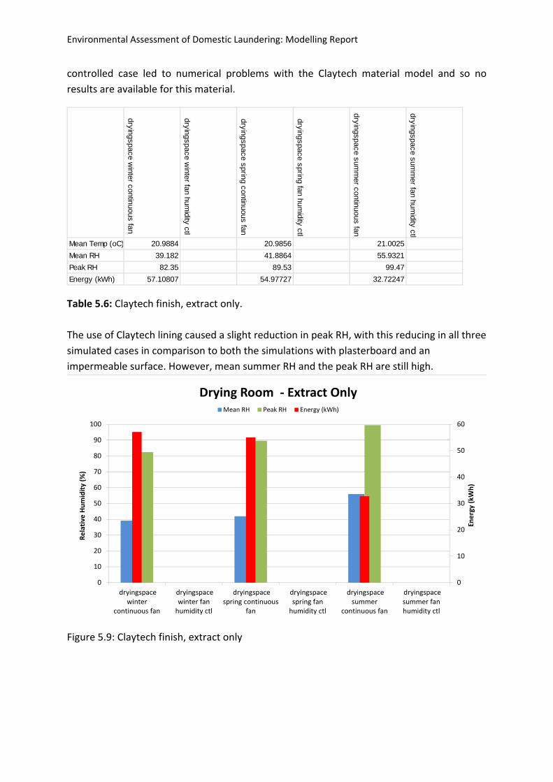
Environmental Assessment of Domestic Laundering: Modelling Report
controlled case led to numerical problems with the Claytech material model and so no
results are available for this material.
Table 5.6: Claytech finish, extract only.
The use of Claytech lining caused a slight reduction in peak RH, with this reducing in all three
simulated cases in comparison to both the simulations with plasterboard and an
impermeable surface. However, mean summer RH and the peak RH are still high.
Figure 5.9: Claytech finish, extract only
dryingspace winter continuous fan
dryingspace winter fan hum
idity ctl
dryingspace spring continuous fan
dryingspace spring fan humidity ctl
dryingspace summ
er continuous fan
dryingspace summ
er fan humidity ctl
Mean Temp (oC) 20.9884 20.9856 21.0025
Mean RH 39.182 41.8864 55.9321
Peak RH 82.35 89.53 99.47
Energy (kWh) 57.10807 54.97727 32.72247
0
10
20
30
40
50
60
0
10
20
30
40
50
60
70
80
90
100
dryingspacewinter
continuous fan
dryingspacewinter fanhumidity ctl
dryingspacespring continuous
fan
dryingspacespring fanhumidity ctl
dryingspacesummer
continuous fan
dryingspacesummer fanhumidity ctl
Energy (kWh)
Relative
Humidity (%
)
Drying Room ‐ Extract OnlyMean RH Peak RH Energy (kWh)
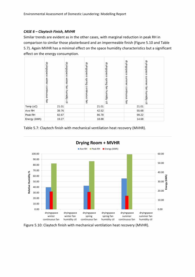
Environmental Assessment of Domestic Laundering: Modelling Report
CASE 6 – Claytech Finish, MVHR
Similar trends are evident as in the other cases, with marginal reduction in peak RH in
comparison to similar those plasterboard and an impermeable finish (Figure 5.10 and Table
5.7). Again MVHR has a minimal effect on the space humidity characteristics but a significant
effect on the energy consumption.
Table 5.7: Claytech finish with mechanical ventilation heat recovery (MVHR).
Figure 5.10: Claytech finish with mechanical ventilation heat recovery (MVHR).
dryingspace winter continuous fan
dryingspace winter fan hum
idity ctl
dryingspace spring continuous fan
dryingspace spring fan humidity ctl
dryingspace summ
er continuous fan
dryingspace summ
er fan humidity ctl
Temp (oC) 21.01 21.01 21.01
Ave RH 39.76 42.52 55.68
Peak RH 82.67 86.78 99.22
Energy (kWh) 19.27 18.88 14.68
0.00
10.00
20.00
30.00
40.00
50.00
60.00
0.00
10.00
20.00
30.00
40.00
50.00
60.00
70.00
80.00
90.00
100.00
dryingspacewinter
continuous fan
dryingspacewinter fanhumidity ctl
dryingspacespring
continuous fan
dryingspacespring fanhumidity ctl
dryingspacesummer
continuous fan
dryingspacesummer fanhumidity ctl
Energy (kWh)
Relative
Humidity %
Drying Room + MVHRAve RH Peak RH Energy (kWh)
Environmental Assessment of Domestic Laundering: Modelling Report
All of the simulations undertaken here indicate that there are potential problems with high
RH in the drying space during the drying period. Further, moisture control surface finishes
had a limited effect on RH; this is likely to be due to the fact that the available surface area
for absorption is small. In summer both mean and peak RH are high; this indicates that the
15 l/s recommended in the draft drying specifications (Menon and Porteous, 2012) may be
inadequate with regards to maintaining acceptable RH levels in the drying cupboard.
Additionally, whilst the humidistat‐based control is effective in reducing the fan energy
consumption, it has a detrimental effect on the RH. Consequently, a further set of
simulations were undertaken in order to 1) analyse the effect of increasing the fan flow rate
to 30 l/s and 2) change the dead band of the fan humidistat‐based controller to 40‐60% in
order to reduce the detrimental effect on RH.
5.2.2 Enhanced Drying Space Ventilation
The following cases were examined.
Drying space supplied with 15 l/s from an MVHR system (80% heat exchanger
effectiveness), with continuous fan operation and with fan subject to humidistatic
ON/OFF dead band control between 40‐60% RH;
Drying space supplied with 15 l/s from an extract only system, with continuous fan
operation and with fan subject to humidistatic ON/OFF dead band control between 40‐
60% RH;
Drying space supplied with 30 l/s from an MVHR system (80% heat exchanger
effectiveness), with continuous fan operation and with fan subject to humidistatic
ON/OFF dead band control between 40‐60% RH;
Drying space supplied with 30 l/s from an extract only system, with continuous fan
operation and with fan to humidistatic ON/OFF dead band control between 40‐60% RH.
For all cases above, moisture absorbing surfaces were not modelled due to their limited
effect on overall RH, as evidenced in Section 5.2.1. This is due to the limited surface area
available in the drying space for absorption of moisture.
The drying room temperature was controlled to 21oC using a heating coil with a 1kW
capacity. The heating requirement accounts for ventilation losses and the energy required
for evaporation. The assumption is that there is heavy use of the drying room, with 1 small
wash per day dried and 2 washes at weekends.
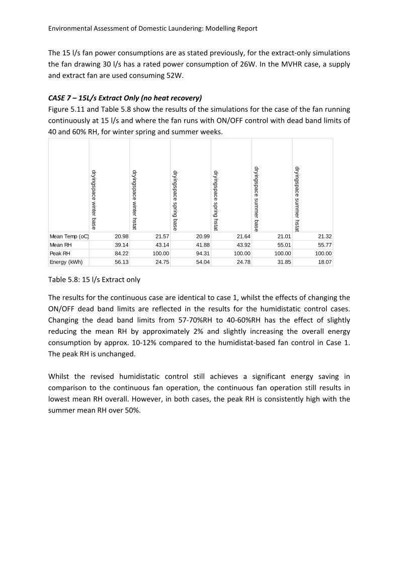
Environmental Assessment of Domestic Laundering: Modelling Report
The 15 l/s fan power consumptions are as stated previously, for the extract‐only simulations
the fan drawing 30 l/s has a rated power consumption of 26W. In the MVHR case, a supply
and extract fan are used consuming 52W.
CASE 7 – 15L/s Extract Only (no heat recovery)
Figure 5.11 and Table 5.8 show the results of the simulations for the case of the fan running
continuously at 15 l/s and where the fan runs with ON/OFF control with dead band limits of
40 and 60% RH, for winter spring and summer weeks.
Table 5.8: 15 l/s Extract only
The results for the continuous case are identical to case 1, whilst the effects of changing the
ON/OFF dead band limits are reflected in the results for the humidistatic control cases.
Changing the dead band limits from 57‐70%RH to 40‐60%RH has the effect of slightly
reducing the mean RH by approximately 2% and slightly increasing the overall energy
consumption by approx. 10‐12% compared to the humidistat‐based fan control in Case 1.
The peak RH is unchanged.
Whilst the revised humidistatic control still achieves a significant energy saving in
comparison to the continuous fan operation, the continuous fan operation still results in
lowest mean RH overall. However, in both cases, the peak RH is consistently high with the
summer mean RH over 50%.
dryingspace winter base
dryingspace winter hstat
dryingspace spring base
dryingspace spring hstat
dryingspace summ
er base
dryingspace summ
er hstat
Mean Temp (oC) 20.98 21.57 20.99 21.64 21.01 21.32
Mean RH 39.14 43.14 41.88 43.92 55.01 55.77
Peak RH 84.22 100.00 94.31 100.00 100.00 100.00
Energy (kWh) 56.13 24.75 54.04 24.78 31.85 18.07
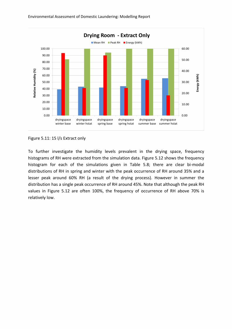
Environmental Assessment of Domestic Laundering: Modelling Report
Figure 5.11: 15 l/s Extract only
To further investigate the humidity levels prevalent in the drying space, frequency
histograms of RH were extracted from the simulation data. Figure 5.12 shows the frequency
histogram for each of the simulations given in Table 5.8; there are clear bi‐modal
distributions of RH in spring and winter with the peak occurrence of RH around 35% and a
lesser peak around 60% RH (a result of the drying process). However in summer the
distribution has a single peak occurrence of RH around 45%. Note that although the peak RH
values in Figure 5.12 are often 100%, the frequency of occurrence of RH above 70% is
relatively low.
0.00
10.00
20.00
30.00
40.00
50.00
60.00
0.00
10.00
20.00
30.00
40.00
50.00
60.00
70.00
80.00
90.00
100.00
dryingspacewinter base
dryingspacewinter hstat
dryingspacespring base
dryingspacespring hstat
dryingspacesummer base
dryingspacesummer hstat
Energy (kWh)
Relative Humidity (%
)Drying Room ‐ Extract Only
Mean RH Peak RH Energy (kWh)
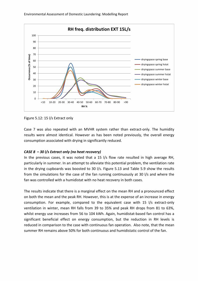
Environmental Assessment of Domestic Laundering: Modelling Report
Figure 5.12: 15 l/s Extract only
Case 7 was also repeated with an MVHR system rather than extract‐only. The humidity
results were almost identical. However as has been noted previously, the overall energy
consumption associated with drying in significantly reduced.
CASE 8 – 30 l/s Extract only (no heat recovery)
In the previous cases, it was noted that a 15 l/s flow rate resulted in high average RH,
particularly in summer. In an attempt to alleviate this potential problem, the ventilation rate
in the drying cupboards was boosted to 30 l/s. Figure 5.13 and Table 5.9 show the results
from the simulations for the case of the fan running continuously at 30 l/s and where the
fan was controlled with a humidistat with no heat recovery in both cases.
The results indicate that there is a marginal effect on the mean RH and a pronounced effect
on both the mean and the peak RH. However, this is at the expense of an increase in energy
consumption. For example, compared to the equivalent case with 15 l/s extract‐only
ventilation in winter, mean RH falls from 39 to 35% and peak RH drops from 81 to 63%,
whilst energy use increases from 56 to 104 kWh. Again, humidistat‐based fan control has a
significant beneficial effect on energy consumption, but the reduction in RH levels is
reduced in comparison to the case with continuous fan operation. Also note, that the mean
summer RH remains above 50% for both continuous and humidistatic control of the fan.
0
10
20
30
40
50
60
70
80
90
100
<10 10‐20 20‐30 30‐40 40‐50 50‐60 60‐70 70‐80 80‐90 >90
Occurrence (% of time)
RH %
RH freq. distribution EXT 15L/s
dryingspace spring base
dryingspace spring hstat
dryingspace summer base
dryingspace summer hstat
dryingspace winter base
dryingspace winter hstat
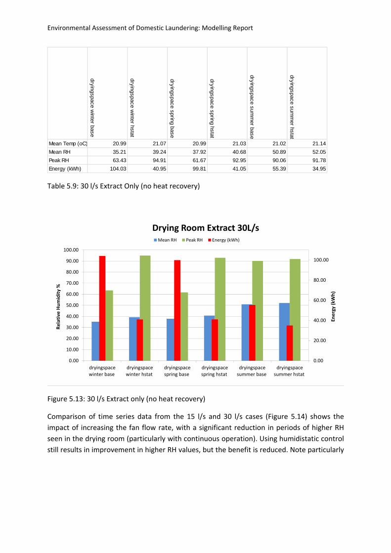
Environmental Assessment of Domestic Laundering: Modelling Report
Table 5.9: 30 l/s Extract Only (no heat recovery)
Figure 5.13: 30 l/s Extract only (no heat recovery)
Comparison of time series data from the 15 l/s and 30 l/s cases (Figure 5.14) shows the
impact of increasing the fan flow rate, with a significant reduction in periods of higher RH
seen in the drying room (particularly with continuous operation). Using humidistatic control
still results in improvement in higher RH values, but the benefit is reduced. Note particularly
dryingspace winter base
dryingspace winter hstat
dryingspace spring base
dryingspace spring hstat
dryingspace summ
er base
dryingspace summ
er hstat
Mean Temp (oC) 20.99 21.07 20.99 21.03 21.02 21.14
Mean RH 35.21 39.24 37.92 40.68 50.89 52.05
Peak RH 63.43 94.91 61.67 92.95 90.06 91.78
Energy (kWh) 104.03 40.95 99.81 41.05 55.39 34.95
0.00
20.00
40.00
60.00
80.00
100.00
0.00
10.00
20.00
30.00
40.00
50.00
60.00
70.00
80.00
90.00
100.00
dryingspacewinter base
dryingspacewinter hstat
dryingspacespring base
dryingspacespring hstat
dryingspacesummer base
dryingspacesummer hstat
Energy (kWh)
Relative Humidity %
Drying Room Extract 30L/sMean RH Peak RH Energy (kWh)
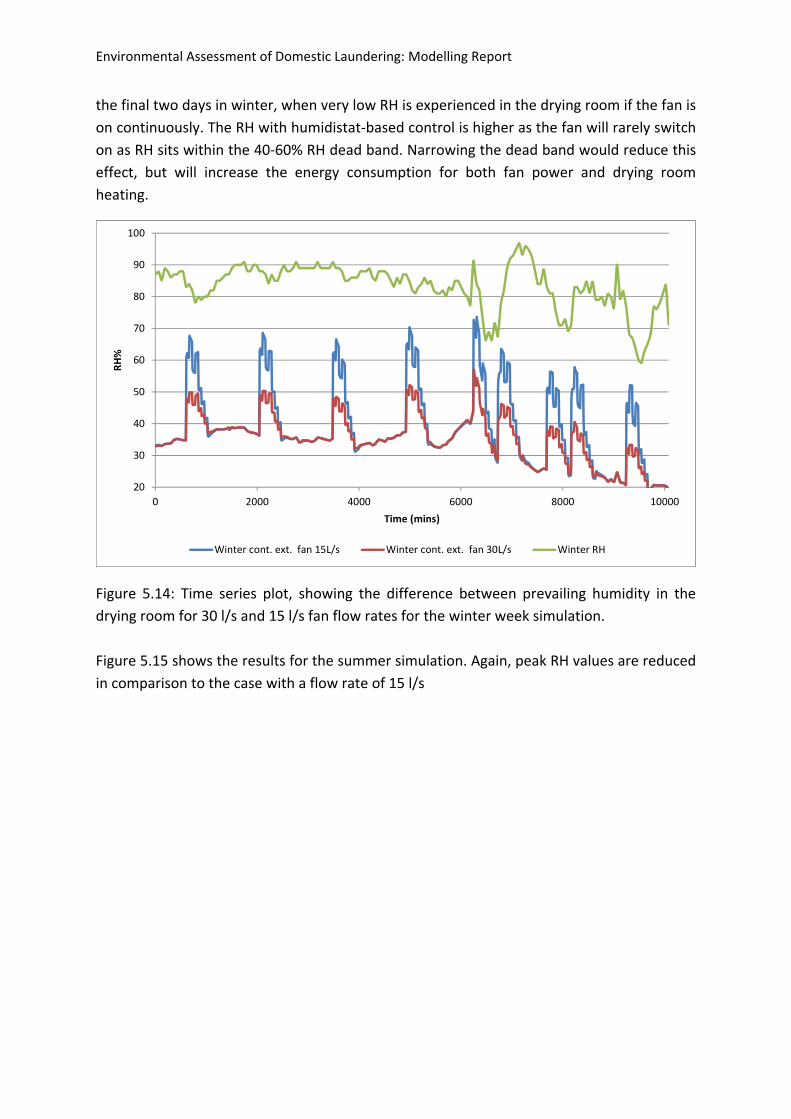
Environmental Assessment of Domestic Laundering: Modelling Report
the final two days in winter, when very low RH is experienced in the drying room if the fan is
on continuously. The RH with humidistat‐based control is higher as the fan will rarely switch
on as RH sits within the 40‐60% RH dead band. Narrowing the dead band would reduce this
effect, but will increase the energy consumption for both fan power and drying room
heating.
Figure 5.14: Time series plot, showing the difference between prevailing humidity in the
drying room for 30 l/s and 15 l/s fan flow rates for the winter week simulation.
Figure 5.15 shows the results for the summer simulation. Again, peak RH values are reduced
in comparison to the case with a flow rate of 15 l/s
20
30
40
50
60
70
80
90
100
0 2000 4000 6000 8000 10000
RH%
Time (mins)
Winter cont. ext. fan 15L/s Winter cont. ext. fan 30L/s Winter RH
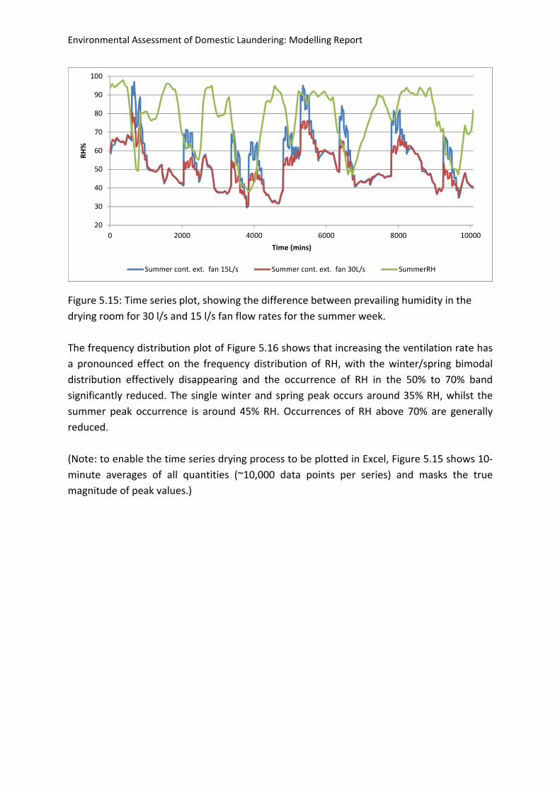
Environmental Assessment of Domestic Laundering: Modelling Report
Figure 5.15: Time series plot, showing the difference between prevailing humidity in the
drying room for 30 l/s and 15 l/s fan flow rates for the summer week.
The frequency distribution plot of Figure 5.16 shows that increasing the ventilation rate has
a pronounced effect on the frequency distribution of RH, with the winter/spring bimodal
distribution effectively disappearing and the occurrence of RH in the 50% to 70% band
significantly reduced. The single winter and spring peak occurs around 35% RH, whilst the
summer peak occurrence is around 45% RH. Occurrences of RH above 70% are generally
reduced.
(Note: to enable the time series drying process to be plotted in Excel, Figure 5.15 shows 10‐
minute averages of all quantities (~10,000 data points per series) and masks the true
magnitude of peak values.)
20
30
40
50
60
70
80
90
100
0 2000 4000 6000 8000 10000
RH%
Time (mins)
Summer cont. ext. fan 15L/s Summer cont. ext. fan 30L/s SummerRH
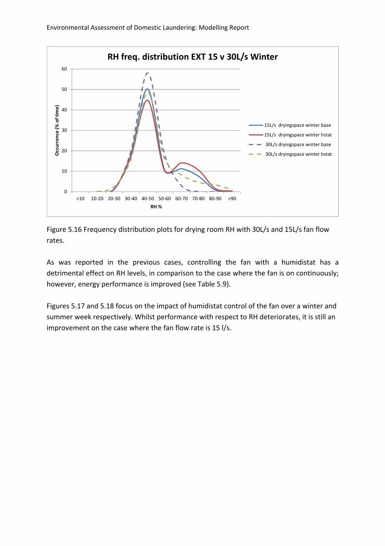
Environmental Assessment of Domestic Laundering: Modelling Report
Figure 5.16 Frequency distribution plots for drying room RH with 30L/s and 15L/s fan flow
rates.
As was reported in the previous cases, controlling the fan with a humidistat has a
detrimental effect on RH levels, in comparison to the case where the fan is on continuously;
however, energy performance is improved (see Table 5.9).
Figures 5.17 and 5.18 focus on the impact of humidistat control of the fan over a winter and
summer week respectively. Whilst performance with respect to RH deteriorates, it is still an
improvement on the case where the fan flow rate is 15 l/s.
0
10
20
30
40
50
60
<10 10‐20 20‐30 30‐40 40‐50 50‐60 60‐70 70‐80 80‐90 >90
Occurrence (% of time)
RH %
RH freq. distribution EXT 15 v 30L/s Winter
15L/s dryingspace winter base
15L/s dryingspace winter hstat
30L/s dryingspace winter base
30L/s dryingspace winter hstat
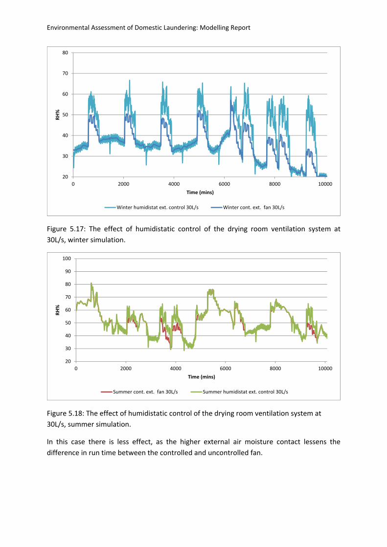
Environmental Assessment of Domestic Laundering: Modelling Report
Figure 5.17: The effect of humidistatic control of the drying room ventilation system at
30L/s, winter simulation.
Figure 5.18: The effect of humidistatic control of the drying room ventilation system at
30L/s, summer simulation.
In this case there is less effect, as the higher external air moisture contact lessens the
difference in run time between the controlled and uncontrolled fan.
20
30
40
50
60
70
80
0 2000 4000 6000 8000 10000
RH%
Time (mins)
Winter humidistat ext. control 30L/s Winter cont. ext. fan 30L/s
20
30
40
50
60
70
80
90
100
0 2000 4000 6000 8000 10000
RH%
Time (mins)
Summer cont. ext. fan 30L/s Summer humidistat ext. control 30L/s
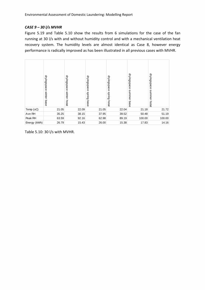
Environmental Assessment of Domestic Laundering: Modelling Report
CASE 9 – 30 l/s MVHR
Figure 5.19 and Table 5.10 show the results from 6 simulations for the case of the fan
running at 30 l/s with and without humidity control and with a mechanical ventilation heat
recovery system. The humidity levels are almost identical as Case 8, however energy
performance is radically improved as has been illustrated in all previous cases with MVHR.
Table 5.10: 30 l/s with MVHR.
dryingspace w
inter base
dryingspace winter hstat
dryingspace spring base
dryingspace spring hstat
dryingspace summ
er base
dryingspace summ
er hstat
Temp (oC) 21.05 22.09 21.05 22.04 21.18 21.72
Ave RH 35.25 38.15 37.95 39.52 50.48 51.19
Peak RH 63.59 92.16 62.98 89.19 100.00 100.00
Energy (kWh) 26.79 15.43 26.00 15.38 17.83 14.16
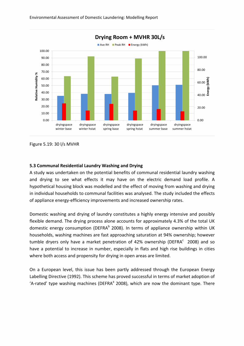
Environmental Assessment of Domestic Laundering: Modelling Report
Figure 5.19: 30 l/s MVHR
5.3 Communal Residential Laundry Washing and Drying
A study was undertaken on the potential benefits of communal residential laundry washing
and drying to see what effects it may have on the electric demand load profile. A
hypothetical housing block was modelled and the effect of moving from washing and drying
in individual households to communal facilities was analysed. The study included the effects
of appliance energy‐efficiency improvements and increased ownership rates.
Domestic washing and drying of laundry constitutes a highly energy intensive and possibly
flexible demand. The drying process alone accounts for approximately 4.3% of the total UK
domestic energy consumption (DEFRAb 2008). In terms of appliance ownership within UK
households, washing machines are fast approaching saturation at 94% ownership; however
tumble dryers only have a market penetration of 42% ownership (DEFRAc 2008) and so
have a potential to increase in number, especially in flats and high rise buildings in cities
where both access and propensity for drying in open areas are limited.
On a European level, this issue has been partly addressed through the European Energy
Labelling Directive (1992). This scheme has proved successful in terms of market adoption of
‘A‐rated’ type washing machines (DEFRAa 2008), which are now the dominant type. There
0.00
20.00
40.00
60.00
80.00
100.00
0.00
10.00
20.00
30.00
40.00
50.00
60.00
70.00
80.00
90.00
100.00
dryingspacewinter base
dryingspacewinter hstat
dryingspacespring base
dryingspacespring hstat
dryingspacesummer base
dryingspacesummer hstat
Energy (kWh)
Relative Humidity %
Drying Room + MVHR 30L/sAve RH Peak RH Energy (kWh)
Environmental Assessment of Domestic Laundering: Modelling Report
has been less success with tumble dryers (DEFRAb 2008), with the market being
predominantly made up of ‘C‐Rated’ machines.
Due to the potential health effects arising from reduced indoor air quality and high internal
humidity levels resulting from indoor drying of laundry, it could be beneficial to shift laundry
washing and drying from individual household owned units to communal washing and
drying appliances within dedicated areas in individual housing blocks. Communal washing
and drying was a common practice in the UK during the 19th century, and today could
possibly prove beneficial in terms of electrical energy demand reductions as well as
changing the temporal nature of electrical demands.
An analysis was undertaken of the effect on the electrical demand profile of a residential
block of flats in a scenario where domestic washing and drying is shifted from the traditional
individual household‐based appliances to a regulated staggered use of communal washing
and drying facilities. The analysis considers the potential of a communal laundry to improve
the electrical demand characteristics of the building through time‐shifting demand and
reducing peak electrical loading, both of which could provide more favourable operating
conditions for low carbon and localised energy supplies.
The methodology used 1‐minute resolution electrical demand profiles for the housing block
under different scenarios for three specific days; a characteristic winter day, a characteristic
summer day and one day representative of the transition months. The three days selected
helped to identify the main trends from shifting to communal laundry facilities at different
times of the year. The use of a 1‐minute resolution for the profiles ensured that certain key
characteristics such as the maximum peak demand and load duration could be clearly
identified. Apart from understanding the difference between the use of individual washing
and drying units and the use of communal facilities this research also aims to analyse other
related aspects, such as the effect of increased demands for drying and the use of more
energy‐efficient technologies. In order to compare the use of individual washing machines
and tumble dryer appliances versus the use of communal units, three scenarios were
considered, namely:
individual use of washing machines and tumble dryers at current ownership rates;
individual use of washing machines and tumble dryers at saturated ownership
rates;
regulated staggered use of communal washing machines and tumble dryers.
Figure 5.20 shows an example of the high frequency analysis.
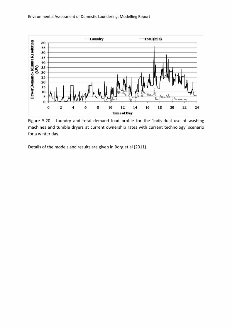
Environmental Assessment of Domestic Laundering: Modelling Report
Figure 5.20: Laundry and total demand load profile for the ‘individual use of washing
machines and tumble dryers at current ownership rates with current technology’ scenario
for a winter day
Details of the models and results are given in Borg et al (2011).

Environmental Assessment of Domestic Laundering: Modelling Report
6. Modelling – realistic case
See note at the end of the report contents.
Environmental Assessment of Domestic Laundering: Modelling Report
7. Conclusions
Software Modifications
Before commencing with the modelling of drying processes in dwellings, a series of
modifications to the ESP‐r simulation tool were undertaken with a view to enhancing its
existing moisture modelling capabilities.
ESP‐r’s database of material moisture transport data was improved, using data from
both IEA research and tests undertaken by projects partners Glasgow Caledonian
University.
Two new moisture transport functions (sorption isotherm functions) were added to
ESP‐r to enable the calculation of the material moisture content. One of these was
specifically developed to model the moisture absorption of aerated concrete.
The source code was modified to incorporate a new vapour permeability function for
gypsum plasterboard.
An existing ESP‐r wetted surface moisture source equation was improved to better
represent the characteristics of clothes drying. The equation predictions were
compared to empirical data.
Finally, parametric test software was developed to enable the ESP‐r tool to be used
in sensitivity analyses involving many hundreds of simulation runs.
Validation Study
To develop confidence in ESP‐r’s predictions of indoor moisture levels and also in its abilites
to model the effect of moisture control materials a series of validation tests were
undertaken. These indicated the following.
Simulation results produced when using a vapour tight internal surface material
showed good agreement when compared to analytical results, emphasising the
accuracy of the internal air moisture balance being carried out by ESP‐r under
isothermal conditions.
A second study looked at the impact of modelling the moisture buffering effect of
the concrete construction. Reasonable agreement was achieved again between the
ESP‐r output and analytical results.
Inter‐model comparison of a vapour permeable construction under dynamic
conditions proved inconclusive as the results from ESP‐r and the solutions provided
by other hygrothermal modelling software showed large degree of variation in
outcomes. However the ESP‐r results tended to be in the middle of the range of
results.
Environmental Assessment of Domestic Laundering: Modelling Report
Comparison of ESP‐r results to empirical test data and the output from other
modelling tools accounting for the effects of ventilation and moisture buffering
material showed reasonable agreement with the measured data and ESP‐r’s results
were consistent with the spread of simulated results from other simulation software.
Finally, modelling of moisture conditions in a realistic dwelling indicated that there
was satisfactory correlation between predicted and actual measured values of peak
humidity. However, differences between the rates of desorption predicted and
measured were apparent. ESP‐r uses an average sorption‐desorption isotherm,
whereas in practice the processes are not symmetrical. Although the required
hygrothermal material data is not always available, it is suggested that future model
developments should include the possibility to use explicit sorption‐desorption
isotherms.
Modelling Studies
Several distinct modelling studies were undertaken. These focused on two areas: the energy
impacts of laundry drying and mechanisms to alleviate poor environmental conditions due
to drying. The conclusions from these activies are as follows.
Communal Laundry Study
This study focused on the potential energy benefits of communal laundering in high
density housing in comparison to the use of separate household appliances. Both
washing and tumble drying are important loads within the total electric load profile
of a household unit or a housing block with an annual average energy intensity of
27% of the total electrical energy consumption of a housing block calculated at
current appliance ownership rates and technologies.
The use of a regulated, staggered system of communal washing/drying rather than
the current practice of using appliances based in each individual household should
lead to a flattening of the electrical load with lower peak demands. This could
improve the matching with local micro‐generation electricity supplies. However,
communal laundering is ineffective in reducing overall electricity consumption.
The increased use of tumble dryers (whether individual or communal) would lead to
a considerable increase in terms of total daily load, average load and load intensity.
To get maximum benefits, the communal use of laundry washing and drying
appliances should be accompanied by a changeover to more energy‐efficient
appliances. Such future reductions in energy intensity of commercial type washing
machines and dryers could add to the benefits of communal facilities.
Environmental Assessment of Domestic Laundering: Modelling Report
Parametric Analysis
A parametric study was undertaken to assess the effect of key parameters on indoor relative
humidity. These included climate, season, moisture load, occupancy, airtightness and
insulation levels. This indicated the following.
Introducing significant areas of moisture absorbing surfaces finish within the building
could have a pronounced effect on peak RH, with absolute peak values dropping by
up to 40%. However, the effect of a dedicated moisture absorbing surface finishes
(e.g. clayboard) did not differ greatly from standard hygroscopic materials such as
plasterboard.
Further, both moisture load and ventilation levels had a more profound effect on the
mean RH.
Significantly, improving the quality of the building fabric also had a beneficial effect
on RH, due to increased indoor temperatures.
Energy and Humkidity Impact of Indoor Clothes Drying
Using the same model, simulations were undertaken to assess the energy impact of indoor
clothes drying techniques identified in the project field trials, where clothing was dried by
opening the windows and the heating systems left on. The outcomes were as follows.
Drying under these circumstances used more than double the energy of a tumble
dryer and resulted in over 20% more carbon emissions (if the space heating is
provided by gas central heating).
Simulations also indicated that the drying of clothes in the living space of a dwelling
would result in high mean RH levels above 60% for significant periods of time.
Dedicated Drying Space
Drying clothing in a dedicated drying space was also investigated in two sets of simulations.
The first looked at the impact of drying clothes in a dedicated space on conditions within the
rest of a simulated house and showed that this dropped the mean RH level to approximately
40%.
Further simulations were undertaken to assess the performance of a dedicated drying space
(volume of 1.75m3) for clothing as set out in the design guide (Menon and Porteous, 2012).
Specifically, measures to reduce the energy penalty associated with drying were analysed
along with the conditions prevailing within the drying space. Consequently, the drying space
Environmental Assessment of Domestic Laundering: Modelling Report
model was modelled with extract only ventilation and mechanical ventilation heat recovery.
The effect of different surface finishes were also examined.
With a fan flow rate of 15 l/s, high mean and peak humidity levels were evident in
both spring and summer simulations, with mean humidities of over 50% evident.
Changing surface finishes from impermeable to permeable materials had a limited
effect on peak and mean RH, probably due to the very limited internal surface area
in the drying space.
The use of humidistat control of the fan (where the fan operated with on‐off control
between deadband limits of 50 and 70% RH) reduced the overall energy
consumption of the drying space significantly, but had a detrimental impact on
humidity control.
The use of mechanical ventilation heat recovery had a beneficial impact on energy
consumption and had little impact on the RH levels in the drying space, reducing
energy consumption by over 60% without MVHR.
Increasing ventilation levels to 30 l/s was successful in reducing occurrences of high
RH in the drying space, though summer RH levels were still high (due to high external
air moisture content) and energy consumption almost doubled in comparison to the
15 l/s case.
Again, humidistat control of the ventilation (this time where the fan operated with
on‐off control between deadband limits of 40 and 60% RH) improved energy
performance at the expense of reduced effectiveness in controlling RH.
A fan flow rate of 30 l/s MVHR reduced overall energy consumption by over 70%
compared to the no‐MVHR case, with no detrimental impact on RH conditions.
Environmental Assessment of Domestic Laundering: Modelling Report
8 References
Borg S, Kelly N, Markopoulos A, Strachan P, Porteous C and Sharpe T, Communal Residential
Laundry Washing And Drying – Can It Provide Demand‐Side Electrical Load Flexibility?, 2nd
International Conference on Microgeneration and Related technologies, Glasgow, April 2011
Clarke J A (2001) Energy Simulation in Building Design (2nd Edition), London: Butterworth‐
Heinemann, ISBN 0 7506 5082 6
Clarke J A and Hensen J L M (1991) ‘An Approach to the Simulation of Coupled Heat and
Mass Flow in Buildings’, Int. J. Indoor Air Quality and Climate, 1, pp283‐96.
Clarke J A and Tang D (2004) ‘A co‐operative solver approach to building simulation’, Proc.
ESIM’04, Natural Resources Canada, Ottawa.
DEFRAa (2008). BNW14: EC Energy Labelling of washing machines, Vol. in Series "Market
Transformation Programme”, DEFRA UK.
DEFRAb (2008). IBNW24: Innovation Briefing Note on domestic laundry drying products, Vol.
in Series "Market Transformation Programme”, DEFRA UK.
DEFRAc (2008). Policy Brief: Improving the energy performance of domestic wet products,
Vol. in Series “Market Transformation Programme”, DEFRA UK.
ESP‐r (2012), http://www.esru.strath.ac.uk/Programs/ESP‐r.htm
European Energy Labelling Directive (1992), Directive 92/75/EEC of 22 September 1992 on
the indication by labelling and standard product information of the consumption of energy
and other resources by household appliances.
Galbraith G H, McLean R C, Jiansong G (1998) ‘Moisture permeability data: Mathematical
presentation, Building Services Engineering Research and Technology, Volume 19, pp31‐36.
Hansen K K (1986) ‘Sorption Isotherms: A Catalogue’ Technical Report 162/86, Technical
University of Denmark.
Hong J, Kelly N J, Johnstone C (2010), Identifying characteristic building types for use in the
modelling of highly distributed power systems performance. HIDEF Briefing Report.
http://www.supergen‐hidef.org/Publications/Pages/Publications.aspx
IEA Annex 14 (1991) Condensation and Energy: Catalogue of Material Properties
http://www.ecbcs.org/annexes/annex14.htm
IEA Annex 24 (1996) Material Properties ‐ Final Report, Volume 3
http://www.ecbcs.org/annexes/annex24.htm
IEA Annex 41 (2005) http://www.ecbcs.org/annexes/annex41.htm
Environmental Assessment of Domestic Laundering: Modelling Report
Markopoulos A, (2102) ‘Integrated Modelling of Moisture Release, Transport and Buffering
in Housing’, PhD Thesis, to be submitted, University of Strathclyde.
Menon R and Porteous C (2012), Design Guide: Healthy Low Energy Home Laundering,
MEARU (Mackintosh Environmental Architecture Research Unit), The Glasgow School of Art
(output from this EPSRC project).
Mujumdar A S (1980), Advances in Drying (Volume 1), Hemisphere Publishing Corporation,
ISBN 0 89116 185 6
Nakhi A E (1995) 'Adaptive construction modelling within whole building dynamic
simulation', PhD Thesis, Glasgow: University of Strathclyde.
Steeman H J, Janssens A, De Paepe M (2009), ‘On the applicability of the heat and mass
transfer analogy in indoor air flows, International Journal of Heat and Mass Transfer,
Volume 52, pp1431‐1442.
Tang R, Etzion Y (2004), Comparative studies on the water evaporation rate from a wetted surface and that from a free water surface, Building and Environment, v39, pp77‐86.
Woloszyn M and Rode C (2007), IEA Annex 41 Subtask 1, Modelling Principles and Common
Exercises, IEA Annex 41 Final Report.