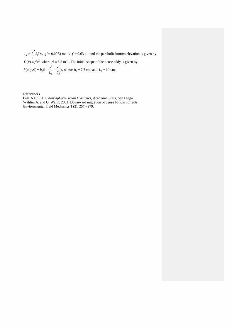
Equation Chapter 1 Section 1 6. QUASI-GEOSTROPHIC DYNAMICS OF DENSE WATER ON SLOPING TOPOGRAPHY The focus of this chapter is on the dynamics of a dense current flowing along a sloping topography, and of its adjustment under gravity, rotation, and bottom friction. Consider a so-called 1.5-layer system, i.e. a well mixed layer with density 0ρ ρ+ ∆ flowing along the bottom beneath a very deep, stagnant layer with density 0ρ (Fig. 1). Assuming that the layer has a small aspect ratio the flow is governed by the shallow water equations with reduced gravity (Gill, 1986; Wåhlin and Walin, 2001),

' ( )Xu u u Fu v fv g h D

t x y x h∂ ∂ ∂ ∂

+ + − = − + −∂ ∂ ∂ ∂

(1)

' ( )Yv v v Fu v fu g h D

t x y y h∂ ∂ ∂ ∂

+ + + = − + −∂ ∂ ∂ ∂

(2)

( )X Yh uh vh m m

t x y x y∂ ∂ ∂ ∂ ∂

+ + = − +∂ ∂ ∂ ∂ ∂

, (3)

where D is the bottom elevation and h is the thickness of the dense layer (Figure 1). Furthermore (u, v) are the horizontal velocity components in the (x, y) directions, f is the

Coriolis parameter and 0

'g g ρρ∆

= is the reduced gravity. Friction is represented either by the

stress ( , )X YF F=F or by the Ekman transport ( , )X Ym m=m created by the stress. Thus either ≡F 0 or ≡m 0 depending on which representation is chosen. In the first case ( ≡F 0 ) the flow consists of two parts; the boundary layer (or Ekman-) transport m and the ’inviscid’ part represented by ( , )u v=u . The total horizontal transport is then given by h +u m . In the latter case ( ≡m 0 ), u represents a vertical mean velocity and the transport vector is given by hu . Given a parameterisation for either F or m , eqs (1) - (3) can be solved as an initial value problem. In section 6.3 a more detailed description is provided of how the Ekman transport and Ekman layer thickness are expressed when a bulk friction description of the bottom stress is used. Most of the examples in this chapter will pertain to the simplified one-dimensional bathymetry

0( )D x D xα= + , (4) where α is a constant. The expression (4) is chosen to resemble a part of the continental slope where the slope is approximately constant and along the same direction. 6.1 The quasi-geostrophic approximation The advective and local acceleration terms in (1) and (2) become small when the plume width

W is large compared to the Rossby radius of deformation, 0'g HRo

f= (where 0H is the

scale thickness of the current). This can be seen by introducing non-dimensional variables according to

0 ˆ ˆ( , ) ( , )u v U u v= (5) ˆ ˆ( , ) ( , )x y W x y= (6)

0 ˆUt tW

= (7)

0ˆ ˆ( , ) ( , )h D H h D= . (8)

Using (5) - (8) in (1) - (2) and dividing by f (ignoring the frictional terms) give 2 1ˆ ˆ ˆ ˆ ˆˆ ˆ ˆ ( )ˆ ˆ ˆ ˆ

u u uu v v B h Dt x y x

ε ε ε ε −∂ ∂ ∂ ∂+ + − = − +

∂ ∂ ∂ ∂ (9)

2 1ˆ ˆ ˆ ˆ ˆˆ ˆ ˆ ( )ˆ ˆ ˆ ˆv v vu v u B h Dt x y y

ε ε ε ε −∂ ∂ ∂ ∂+ + + = − +

∂ ∂ ∂ ∂, (10)

where 0UfW

ε = is the Rossby number, and 2 02 2

'g HBf W

= is the Burger number. If the Rossby

number ε is small, then the inertial terms are negligible compared to the Coriolis terms. Physically meaningful solutions require that if 1ε , then the pressure gradient force must be of the same order of magnitude as the Coriolis terms, i.e. that 2 1B or

2 1 21B Bε ε− ≈ ⇔ ≈ . (11) If (11) is not true the momentum equations (9) - (10) degenerates to the trivial solution

ˆ ˆ( , ) 0u v = . Expression (11) tells us that if the current is wide compared to the Rossby radius (i.e. 2 1B ) then the Rossby number ε will be small and the velocity close to geostrophic. Using (5) - (8) in (3) (ignoring the frictional terms) and dividing by 0 0H U gives

ˆ ˆ ˆˆ ˆ0ˆ ˆ ˆ

h uh vht x y∂ ∂ ∂

+ + =∂ ∂ ∂

. (12)

Often the quasi-geostrophic approximation is accompanied with a linearization of h in the continuity equation. Sometimes the linearization is considered to be a part of the quasi-geostrophic approximation, and the flow regime where (12) is not linearized but the approximation 1ε still utilized is termed semi-geostrophic approximation. It is also known as large-amplitude geostrophic motion (Swaters 1991). An important aspect of the role of topography can be shown by utilizing the semi-geostrophic approximation, i.e. by assuming that frictional effects are negligible and that 1ε . Inserting (9) and (10) in (12), ignoring terms of order ε or smaller gives (after reverting back to dimensional parameters)

' ' 0h g D h g D ht f x y f y x

∂ ∂ ∂ ∂ ∂+ − =

∂ ∂ ∂ ∂ ∂. (13)

Equation (13) tells us that if the bathymetric variations are comparable to the thickness of the dense layer, and the flow is not parallel to the depth contours, then there is a first-order time development in the system. This time development is much faster than the quasi-geostrophic adjustment or the frictional adjustment.

On a flat bottom we have 0D Dx y

∂ ∂= =

∂ ∂ and (13) reduces to

0ht

∂=

∂. (14)

Hence there is no first-order time dependence if the bottom is flat, a consequence of what is sometimes called ‘geostrophic degeneracy’ (see e.g. Pedlosky 1987, chapter 2.10). The term refers to the fact that there is a stationary geostrophic velocity field corresponding to each distribution of h. Any time dependence observed in a geostrophic flow on a flat bottom is caused by higher-order dynamics, i.e. the ageostrophic effects induced either by friction or inertial acceleration. Accordingly a dense circular eddy spreads symmetrically under the

influence of bottom friction (Gill et al. 1979; see also Huppert 1982), while the inertial accelerations induce baroclinic instabilities at the edges of the eddy. The instabilities grow in dense eddies on a flat bottom (Saunders 1973) as well as buoyant eddies in a denser environment (Griffiths & Linden 1981), and are also observed when the eddy is created by a constant flux of water from a localized source (Griffiths & Linden 1981) or by cooling of water from above (e.g. Jacobs & Ivey 1998; Legg & Marshall 1993). 6.2 Forward motion induced by sloping topography Consider now the case when the bottom slopes, and the dense layer is not aligned parallel to

the bottom (if the flow is parallel to the bottom we have 0D h D hx y y x

∂ ∂ ∂ ∂− =

∂ ∂ ∂ ∂). Then equation

(13) is not degenerate, and it resembles the wave equation for long baroclinic Rossby waves. However, (13) is valid for large amplitude motions of h; and describes how the water mass itself propagates forward along the topography with the speed of a long Rossby wave. In

quasi-geostrophic theory it is assumed that ht

∂∂

is small compared to the geostrophic

velocities, in which case (13) reduces to the constraint that the flow must follow depth contours (see e.g. Pedlosky, 1987, p. 89). When large-amplitude variations are allowed this constraint is relaxed. In fact, a consequence of (13) is that the flow can be orthogonal to depth contours, as long as it translates along the slope. Given an initial distribution then h evolves in time. However, information can only propagate in the along-slope direction, with shallow water to the right (in the Northern Hemisphere). It is possible to prescribe a distribution of h at an upstream location (but not at a downstream location). Such a boundary condition represents a source for dense water and produces an advancing front, which moves into new ground, establishing a stationary current parallel to the depth contours behind it. The depletion of a current may also be simulated by prescribing that h = 0 at an upstream location. Using the simplified bathymetry (4), (13) can be rewritten to

0Nh hvt x

∂ ∂− =

∂ ∂, (15)

where '

Ngv

fα

= (16)

is the Nof velocity. Since α is constant, (15) has analytical solutions that can be written ( , , ) ( ) ( )h x y t F G xη= , (17)

where Nv t yη = − .

The functions F and G are determined from the initial condition, i.e. ( , ,0) ( ) ( )h x y F y G x= − .

Expression (17) represents a similarity solution to (13) that describes how the water mass translates along the topography, parallel to the depth contours, with the speed Nv . If Nv is not constant, e.g. if the slope increases or decreases with distance from the coast, the forward motion of the front will be faster in regions with steeper bathymetry. It is the shape of the bottom that determines the time development and not the shape of the water mass (and associated geostrophic velocities). This means that the water will move away along the topography in the regions where the bottom slopes, even though it is not forced or pumped in any way.

As an example, consider a circular eddy placed on the constantly sloping bottom described by (4). This problem was first considered by D. Nof (Nof, 1984), which is why the velocity Nv (16) is often referred to as the Nof velocity. The initial distribution of h is then given by

2 2

2 2

0 0( , )x yR Rh x y H e

− −= . (18)

The similarity variable η is then given by 'g t yfαη = − . (19)

From (18) we can find the functions F and G; 2

2

0

xRF H e

−= (20)

2

2yRG e

−= , (21)

which gives the solution 2

2

2 2

'( )

0( , , ) ( ) ( )

g t yx fR Rh x y t F G x H e

α

η

−− −

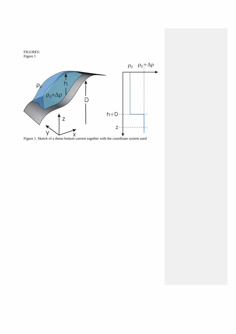
= = . (22) Expression (22) describes how circular eddies move forward along the topography with the Nof speed (16). A second example is shown in Figure 2 where the front of a large-amplitude geostrophic flow advances into a submarine canyon, and how it is depleted after the dense source has been shut off. As can be seen, the current flows along the edges of the canyon, stays at a constant depth and re-emerges on the other side unchanged. 6.3 Effects of bottom friction 6.3.1 Different representations of bottom friction. Bottom friction can be represented either as a bulk 'force' F, or as the boundary layer transport,

Em , which it induces. The two approaches will here be compared. In both cases, the frictional transport is confined to a thin layer next to the bottom, the Ekman boundary layer (δ ), and directed to the left of the flow velocity (in the Northern Hemisphere). In the case of a 'bulk' force representation this transport vanishes outside the plume, where h = 0 and no dense water is to be found. The boundaries, i.e. the regions where the isopycnals intersect the bottom, are part of the solution and develop in time as described by the governing equations. For classical Ekman theory (see e.g. Pedlosky, p. 200), it is assumed that the plume thickness is large compared to the Ekman layer depth. This approach gives an Ekman transport that is independent of the plume thickness, which is obviously wrong when 0h → . As a consequence of this inconsistency the edge regions develop symmetrically according to the frictional smoothing, and there is no difference in the adjustment of the upper and the lower lateral boundary. In order to compare the boundary layer and the bulk force descriptions, consider first the case when the bottom stress is represented by the boundary layer flux m and accordingly F ≡ 0. In

this case ( , )u v represent only the ‘interior’ part ( , )G Gu v of the flow given by 0Gu = (23)

' ( )Ggv h Df x∂

= +∂

(24)

From the Ekman boundary layer theory (Pedlosky [11], p. 200) we have ( , )G Gv vδ δ= − −m (25)

where

2 fνδ =

and ν is the kinematic viscosity. Accordingly

(1 )

G

G

u vh

v vh

δ

δ

= −

= − (26)

where ( , )u v represent vertical mean velocity components. Next consider the case when bottom stresses are represented as the internal force F acting on the bulk of the flow. In this case ( , )u v directly represent vertical mean values of the velocity components. From (30) and (31) the velocities are obtained as

21

2

21

2

(1 )

(1 )

G

G

u vh h

v vh

δ δ

δ

−

−

= − +

= + (27)

where Kf

δ = and K is defined by K=F u (28)

or

DCf

δ =u

and DC is defined by DC=F u u . (29)

Note that δ as described by (29) is not a constant value. It is a parameter that describes the

relative magnitudes of the frictional force and the Coriolis force, hδ . Figure 3 shows the

behaviour of the velocity components ( , )u v for varying δ/h as calculated from (27). The flow components become equally large and half the maximum velocity when δ = h. Furthermore the geostrophic velocity represents an upper bound for the speed in the entire range of bottom stress. Choosing 33 10DC −= ⋅ and 10.3 msGv −= a typical value for δ is calculated as

34

0.33 10 7 m10DC

fδ −

−= = ⋅ =u

. Given that the plume thickness is typically of order 150 m it

can be expected that 0

1Hδ , i.e., that the frictional transport is small compared with the flow

along the isobaths. Accordingly a first-order description of the flow in the interior is obtained by simply ignoring the influence of friction. Close to the lateral boundaries such a description will inevitably break down when h becomes small enough. The time development of a one-dimensional current (i.e. with d/dy = 0) will here be used to show the mechanisms of the downward motion that the Ekman transport induces. Through a change of variables the results can be extended to the case of a stationary current that adjusts along the slope (see eg. Wåhlin and Walin, 2001). For the one-dimensional case, ∂/∂y ≡ 0 and (again ignoring terms of order ε or smaller) (9) - (12) reduce to

1' ( ) Xfv g h D F hx

−∂− = − + −

∂ (30)

1Yfu F h−= − (31)

( ) xh hu mt x x

∂ ∂ ∂+ = −

∂ ∂ ∂. (32)

We will now study the time development of an initial distribution of h on an idealised topography (4). Three different ways of parameterizing bottom friction will be considered; An Ekman boundary layer description according to (23) - (25), and a bulk parameterisation according to (27) which may be either linear or quadratic. 6.3.2. Ekman boundary layer description With =F 0 expressions (30) - (32) give the following equation for the depth distribution,

2

2

h ht x

κ∂ ∂=

∂ ∂. (33)

This is an ordinary diffusion equation with κ given by 'gfδκ =

As described by (33), an initial distribution of h spreads in both directions to minimise the curvature of h (Figure 4). There is no difference between upslope and downslope and consequently no downward migration. Furthermore, there is no consistent loss of potential energy in the system. For certain depth distributions the energy may in fact increase with time. These unexpected results are caused by the fact that it is the lateral variation of the Ekman transport that gives the time development of the flow, and it does not matter which direction the Ekman transport has. According to (26) the Ekman transport is given by

' ( )Xgm h D

f xδ ∂

= +∂

,

which has the unphysical quality that the flow continues outside the plume where h = 0 and no dense water is present. Clearly this is unphysical and the boundary layer flux should tend to zero as the fluid layer vanishes. 6.3.3. Linear bulk stress Assume now that m = 0 and that the stress F in (30) and (31) can be described by the linear bulk parameterisation (28). Inserting (28) in (27) and (32) gives

2

2( ) ( ) '( ) ( ) ( )L Lh q h h D q h h D h Dt x x x x

κ κ ∂ ∂ ∂ ∂ ∂ = + = + + + ∂ ∂ ∂ ∂ ∂

, (34)

where 2

2 2Lhq

h δ=

+, (35)

2

2 2 2

2'( ) ( )( )L L

d hq h q hdh h

δδ

= =+

, (36)

'gfδκ = and K

fδ = . (37)

Figure 5 shows a plot of ( )Lq h and '( )Lq h as functions of h. As can be seen, ( )Lq h behaves like a smooth step function and approaches one for h δ , with the derivative '( )Lq h being non-zero only for h δ< . From (34) two processes that affect the time development of h can be identified:

(i) a diffusive smoothing of h away from the edges, i.e. in the regions where h δ (and hence ( ) 1Lq h ≈ and '( ) 0Lq h ≈ ). In this region the last term on the right of (34) dominates; (ii) a term which contributes close to the boundaries of the plume where h δ< , i.e., where (36) is nonzero. Results obtained from integrations of (34), with the topography (4), are shown in Figure 6 and demonstrate three distinct features: (i) At the upper (landward) edge, the dense interface becomes almost horizontal. Consequently the geostrophic velocities as well as the fricitonal transport there are small, and the downward motion is slow. The edge remains stagnant until the frictional smoothing process starts to affect it. (ii) At the lower (seaward) edge, a thin layer moves downhill with constant speed. The thickness of this layer is comparable to δ and its downward velocity is comparable to the along-slope velocity Nv . (iii) In the interior, friction acts as a diffusive process which minimizes the curvature of the dense layer surface. As a result the current spreads out and the upper boundary begins to move downward. From energy considerations the asymmetric behaviour of the boundaries is important. Ekman suction redistributes fluid from the interior to the lower boundary. Consequently the bulk part of the flow loses potential energy. Without lateral boundaries and the asymmetric behaviour outlined here the dense water spreads out symmetrically over the slope. It can be concluded that the edge regions contribute to a systematic decrease of the potential energy. The behaviour of the boundaries can be understood from the form of the '( )Lq h term in (34) which acts as a source term close to the edges of the plume where h δ< . At the upper boundary the concentrated source (or sink) is quickly wiped out. This is possible since the interface becomes nearly horizontal, with small geostrophic velocity as well as boundary

layer transport. At the lower edge this possibility is not available. The slope ( )h Dx∂

+∂

which

controls the geostrophic flow and thereby the boundary layer transport can not be smaller than the slope of the bottom itself. Accordingly the bottom boundary layer flux remains at full strength all the way down to the region where h becomes smaller than δ. The structure adjusts by widening the region where the outflow from the boundary layer takes place. This is accomplished by sending out a tail with slowly varying depth down the slope. Some precaution is required in the numerical solution of (34). Since '( ) 0Lq h → when 0h → ,

the front needs to be infinitely steep so that '( ) 0̀Lhq hx∂⋅ ≠∂

in order to move forward into new

ground. The problem is avoided if vertically integrated equations are considered. 6.3.4. Quadratic drag law The most widely used friction parameterisation of the three alternatives considered here is the quadratic drag law given by (29). A typical value assigned to the coefficient DC is

33 10DC −= ⋅ . For m = 0 and DC=F u u , (27) and (32) can be written

' ( ) DCfv g h D ux h∂

− = − + −∂

u (38)

DCfu vh

= − u (39)

( ) 0h uht x

∂ ∂+ =

∂ ∂. (40)

where 2 2u v= +u . A governing equation containing only h can be obtained through the

following procedure. Firstly, u is eliminated from (38) - (39) to give 2 2

Gu v vv+ = , (41) where Gv is the geostrophic velocity. Secondly the square of (39) yields

22 2 2 2 2

2 ( )DCf u u v vh

= + ,

which when used with (17) gives a second-order algebraic equation for v with the two roots 1,2v , where

1,2

2

2

( )

( ) 12 4

G

G G G

D GG

v v r h

h h hr h

C vf

δ δ δ

δ

=

= − ± +

=

(42)

Note that Gδ deviates from δ as defined in (37). The point is that Gδ is expressed in terms of

h (i.e., hx∂∂

) since a closed equation for the depth is aspired. From (41) it follows that v and

Gv must have the same sign and consequently the positive root in (42) should be chosen. Making use of (42), (41) and the fact that u has the opposite sign of Gv [cf. (39)], the downward transport is obtained as

( )

( ) ( )(1 ( ))

Q Q G

QQ

uh q h vhq h r h r h

δ

δ

= −

= − (43)

Inserting (43) and (42) in (40) gives the aspired equation for h, ' ( )( )Q

h g h Dq ht f x x

∂ ∂ ∂ +=

∂ ∂ ∂. (44)

The function ( )Qq h has been plotted in Figure 5. Despite the rough appearance, the function ( )Qq h is similar to ( )Lq h . They are both smooth stepfunctions that approach unity for h δ .

Accordingly, similar behaviour of the boundary regions is obtained for the quadratic drag law as for the linear, with the horizontal surface at the upper edge and the widening sheet of dense water leaking out from the lower edge. This is shown in Figure 7 where (44) has been integrated with DC chosen according to

DC v Kα = , (45) where

'N

gvfα

= (46)

is the Nof velocity. This implies similarity between the quadratic and linear parameterisations

when h δ and hx

α∂∂ . The result shown in Fig. 7 closely resemble what was obtained

with the linear description. A minor difference shows up in that the downward migrating layer on the downslope side is somewhat thinner for the quadratic parameterisation. 6.4. Effects of topographic corrugations, canyons and ridges The topography is often ‘wrinkled’ in the along-slope direction, and these small-scale topographic features can have a large effect on the plume dynamics. They channel the dense water and provide a mechanism other than Ekman drainage that makes it possible for the dense water to flow towards the deep sea. Depending on the size of the corrugations, the channelled transport can greatly exceed the Ekman transport. In a purely geostrophic flow the dense water will simply be advected along the topography out of the canyon (Fig. 2). A viscous current however has a frictional transport directed to the left of the velocity, i.e. in towards the centre of the canyon. The canyon in Fig. 2 consequently receives dense water from several directions. As a result, water accumulates and a stationary current going downhill inside the canyon forms. The plume thickness inside the canyon can be considerable, even compared to the frictional boundary layer depth. In order to examine the effect of topographic corrugations on the slope more closely, the straight slope (4) is replaced with a slope that has a topographic 'wrinkle, i.e.

( , ) ( )D x y x d yα= + (47)

where d(y) is a topographical feature, e.g. a ridge or canyon, intersecting an otherwise constantly sloping shelf. The parameter α is the shelf slope angle as before. Figure 8 shows a flow As described in 6.3, bottom friction can be represented either as a bulk drag force acting on

the main flow, or by resolving the Ekman spiral. Both approaches give dynamically similar

results if the magnitude of the drag coefficient is chosen such that the net frictional force is

equal in the different representations (Wåhlin and Walin, 2001). For the sake of simplicity,

we chose the linear drag law representation described in Section 6.3.3.

Assume now that

0hx∂

=∂

, (48)

i.e. that 'G

gvfα

= and transports and velocities do not vary along the ridge/canyon. With the

bathymetry (47) and under assumption (48), the momentum- and continuity equations (30) -

(32) now become 1'fv g Kuhα −− = − − (49)

1' ( ) Yfu g h d F hy

−∂= − + −

∂ (50)

( ) ( ) xh hu hv mt x y x

∂ ∂ ∂ ∂+ + = −

∂ ∂ ∂ ∂. (51)

Since the along-ridge transport does not vary with x, continuity hence requires that

0hv = (52)

or

( )( ) 0L G Gq h hv uδ+ = ,

i.e.

h d hy

α αδ

∂ +− = −

∂ (53)

The solution to (53) has previously been found for a number of different channel topographies

(e.g. Wåhlin, 2004; Davies et al, 2006; Borenäs et al, 2007; Umlauf and Arneborg, 2009) as

well as submarine canyons (Wåhlin, 2002; Muench et al, 2009) and ridges (Darelius and

Wåhlin, 2007). The solution for a vee-shaped channel (Davies et al, 2006) can be written as:

( ) ( )

( ) 01

012

≥

+=

<

−+=

xAexh

xeAxh

x

x

δφ

δφ

φδα

φδα

(8)

where h is the thickness of the outflowing dense layer, φ is the along-channel interface slope

and A is an integration constant determined from boundary conditions. Horizontal integration

of vh across the channel gives the along-channel transport flux Q according to

( )

( )

−−+−−=

′=+== ∫ ∫∫

AAAQ

appendixseeAQfgdxvhdxvhdxvhQ

F

aF

bb

a

21ln22

)1(0

2

22

0 φαδ

(9)

where integral limits x = a and x = b are the interface/side-slope intersections (as defined in

Section 5.1 and Fig. 2). In order for the transport to be real and positive, it is required that

1 0A− ≤ ≤ . The function ( )FQ A increases monotonically from zero at A = -1 to infinity at A

= 0.

Exercises: 1) Show that the time development of a large-amplitude geostrophic eddy which is placed in a

parabolic shaped channel is given by 2 2

0 2 2( , , ) (1 )B B

xh x y t hL Lη

= − − , where Ntu yη = − ,

Comment [A. K. W.1]: This is only a very rough draft text! Look at the figure 8 instead...

' 2Ngu xf

β= , 2' 0.0073 msg −= , 10.63 sf −= and the parabolic bottom elevation is given by

2( )D x xβ= where 15.5 mβ −= . The initial shape of the dense eddy is given by 2 2

0 2 2( , ,0) (1 )B B

y xh x y hL L

= − − , where 0 7.5 cmh = and 10 cmBL = .

References. Gill, A.E.: 1982, Atmosphere-Ocean Dynamics, Academic Press, San Diego. Wåhlin, A. and G. Walin, 2001: Downward migration of dense bottom currents. Environmental Fluid Mechanics 1 (2), 257 - 279.

FIGURES: Figure 1

Figure 1. Sketch of a dense bottom current together with the coordinate system used

Figure 2

Time development of an (a) advancing and (b) retreating dense current. From Wåhlin, 2002.

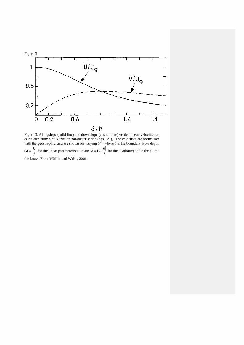
Figure 3

Figure 3. Alongslope (solid line) and downslope (dashed line) vertical mean velocities as calculated from a bulk friction parameterisation (eqs. (27)). The velocities are normalised with the geostrophic, and are shown for varying δ/h, where δ is the boundary layer depth

( Kf

δ = for the linear parameterisation and DCf

δ =u

for the quadratic) and h the plume

thickness. From Wåhlin and Walin, 2001.

Figure 4

Figure 4. Time development of the upper surface of the dense current using the standard Ekman layer description described in Section 6.3.2. The initial height distribution is indicated by the dashed line. The bottom slope is α = 0.01, the reduced gravity g' = 0.02 ms-2 and f = 10-

4 s-1. The boundary layer thickness (dotted line) is (a) δ = 10 m and (b) δ = 80 m. The height is displayed for t = 0, 7 and 14 h.

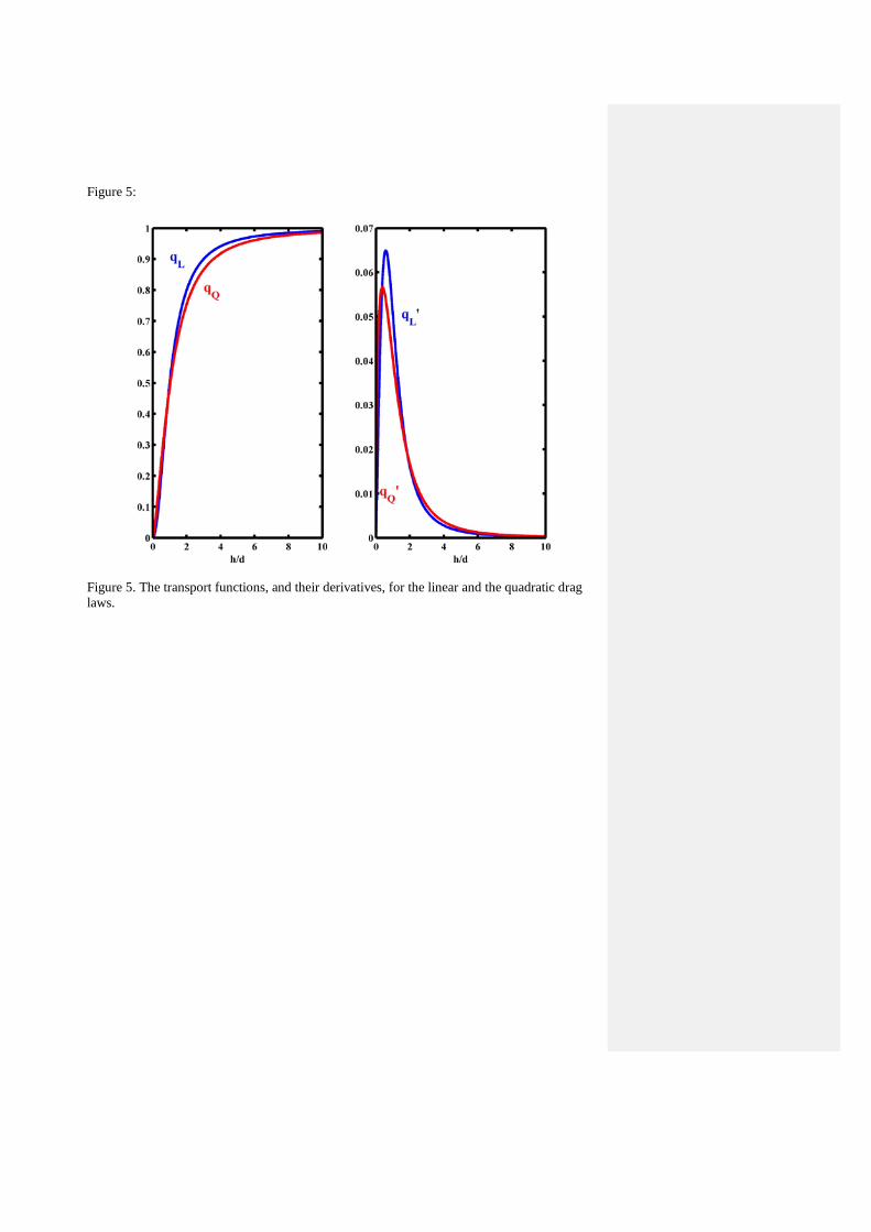
Figure 5:

Figure 5. The transport functions, and their derivatives, for the linear and the quadratic drag laws.

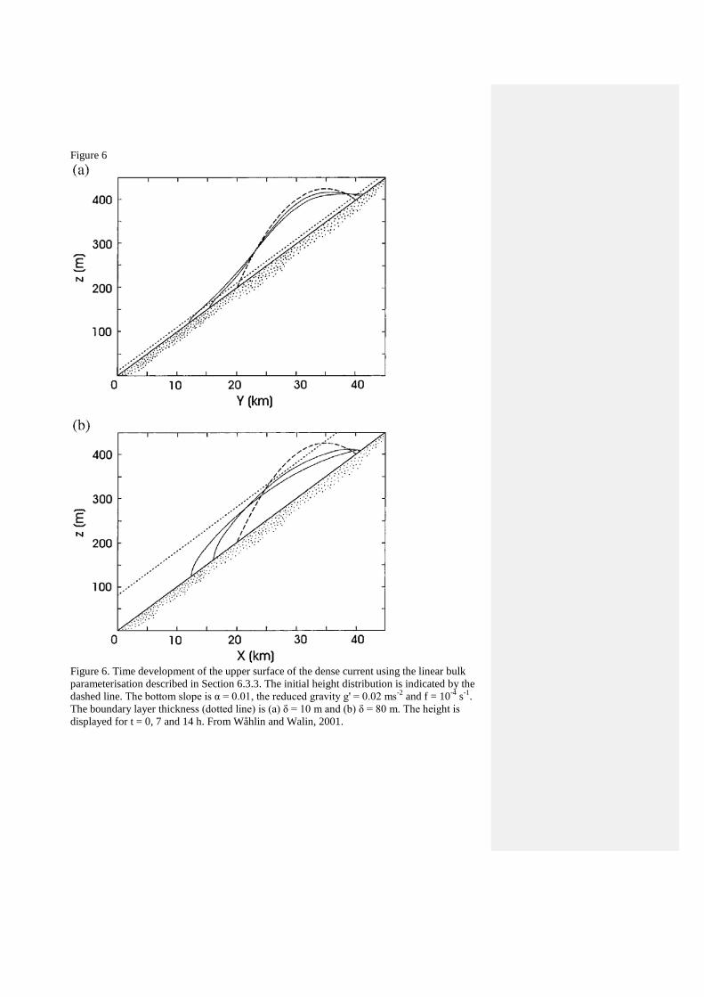
Figure 6

Figure 6. Time development of the upper surface of the dense current using the linear bulk parameterisation described in Section 6.3.3. The initial height distribution is indicated by the dashed line. The bottom slope is α = 0.01, the reduced gravity g' = 0.02 ms-2 and f = 10-4 s-1. The boundary layer thickness (dotted line) is (a) δ = 10 m and (b) δ = 80 m. The height is displayed for t = 0, 7 and 14 h. From Wåhlin and Walin, 2001.

Figure 7

Figure 7. Time development of the upper surface of the dense current using the quadratic bulk

parameterisation described in Section 6.3.4. The boundary layer thickness ( 'DG

C gf fα

αδ = ) is

(a) Gαδ = 10 m and (b) Gαδ = 80 m. The height is displayed for t = 0, 7 and 14 h.

Figure 8:

Something counteracts the geostrophic tendency…

Geostrophic flow is parallell to depth contours, i.e. out of canyon area:

But instead, dense water channeled downhill, trapped in corrugations

Figure 9:

Inside the canyon/corrugation:

From Davies et al, 2006

Flow downhill inside the canyon induces Ekman transport to the left, i.e. opposing the geostrophic flow out of the canyon

Inside the canyon/corrugation:

When downhill flow is sufficiently fast, the two cross-canyon flows (geostrophic and Ekman) cancel.