NASA Technical Memorandum 102246 .

Equations of Motion of Slung Load Systems with Results for Dual Lift Luigi S. Cicolani and Gerd Kanning

February 1990

National Aeronautics and Space Administration

( N A q A - T M - 1 0 7 i 4 6 ) Er3UATIUqS O f M O T I O N O f SLUNG L’IAf‘ S Y S T F M 5 W I T H K E S U L T S FOR O U A L L I F T ( N A C A ) 40 n C S C l . OlC

N90- 17641

Uncl a s G 3 / 0 $ 02b5000

https://ntrs.nasa.gov/search.jsp?R=19900008325 2018-06-16T03:58:44+00:00Z

NASA Technical Memorandum 102246

.

Equations of Motion of Slung Systems with Results for Load

Dual Lift Luigi S. Cicolani and Gerd Kanning, Ames Research Center, Moffett Field, California

February 1990

National Aeronautics and !$ace Administration

Ames Research Center Moffett Field, California 94035

TABLE OF CONTENTS

Page - SUMMARY ................................................................................. 1

SYMBOLS .................................................................................. 2 .r

1. INTRODUCTION. ....................................................................... 5 1.1 Problem Background.. ............................................................ 5

1.2 Equations of Motion for Slung Load Systems.. ..................................... 1.3 Equations of Motion for Multibody Systems.. ......................................

5

8

2. SYSTEM DESCRDPTION ................................................................ 9

3. EQUATIONS OF MOTION OF GENERAL SLUNG LOAD SYSTEMS .................... 10 3.1 Configuration Vectors.. ........................................................ 10 3.2 Kinematics .................................................................... 11 3.3 Equations of Motion from D’ Alembert’s Principle. .............................. 12 3.4 Equations of Motion for Inelastic Suspension: Method 1 . . ....................... 14 3.5 Equations of Motion for Inelastic Suspension: Method 2.. ........................ 17 3.6 Procedure for Generating Simulation Equations ................................. 19

4. DUAL LIFT SIMULATION EQUATIONS ................................................. 21

5. CONCLUSIONS .......................................................................... 30

APPENDIX: SKEW-SYMMETRIC MATRICES AND COORDINATE TRANSFORMATIONS .................................................................. 31

REFERENCES .............................................................................. 34

PRECEDING PAGE BLANK MOT FILMED iii

SUMMARY

This report on the formulation of simulation equations for slung load systems is motivated by an interest in trajectory control for slung loads carried by two or more helicopters. A realistic, analytically simple and computationally efficient set of equations for use in control designs based on inversion of the nonlinear model is of special interest, in addition to the usual requirements for simulation and linear system analysis.

Previous simulations and control analyses of single helicopter systems have used case-specific equa- tions derived from the Newton-Euler equations for rigid bodies or Langrange’s equations for general dy- namic systems. However, the dual lift and multilift systems are more complex, and a more efficient ap- proach tailored to slung load systems appeared essential to obtain tractable working equations, especially in the case that the suspension is assumed inelastic.

In this report, the slung load systems are viewed as systems of rigid bodies connected by straight line cables or links which can be assumed elastic or inelastic. Both assumptions are of interest. The formula- tion for elastic suspensions has been preferred in simulations, owing to its simplicity and computational efficiency. The inelastic cable assumption has been preferred in trajectory coiitrol analyses, in order to eliminate states representing the small, higher frequency motions due to cable stretching. The conventional formulation for inelastic cables eliminates cable forces and cable stretching coordinates at the expense of increased complexity and computational requirements. These negative factors have not impeded the linear control analysis for single helicopter slung load systems, but are a greater obstacle for multilift system analysis and for nonlinear control designs.

Equations are derived using D’ Alembert’s principle and introducing generalized velocity coordinates. Three formulations are derived for general slung load systems. The first two generalize the previous case- specific results for elastic and inelastic suspensions. The third is a new formulation for inelastic suspensions derived from the elastic suspension equations by choosing the generalized coordinates for the elastic system so as to separate motion due to cable stretching from that with fixed cable lengths. The new formulation is significantly more efficient than the conventional one; it is computationally efficient for multibody systems with only a few constraints such as the slung load systems, and a compact analytical form of the nonlinear dynamics is obtained by appropriate selection of the generalized velocity coordinates. Further, it is readily integrated with the elastic suspension formulation in a single simulation, and readily applied to the complex dual lift and multilift systems.

These results are applied to obtain simulation equations for the four-body dual lift system with spreader bar. Two other dual lift suspension arrangements of interest with three bodies are special cases and can be integrated with the four body system in a single simulation. The results are given as vector equations in a programmable form expressed entirely in terms of the natural vectors and matrices of rigid body dynamics. This provides a tractable set of equations for analysis and programming.

PRECEDING PAGE BLANK NOT FiLMED

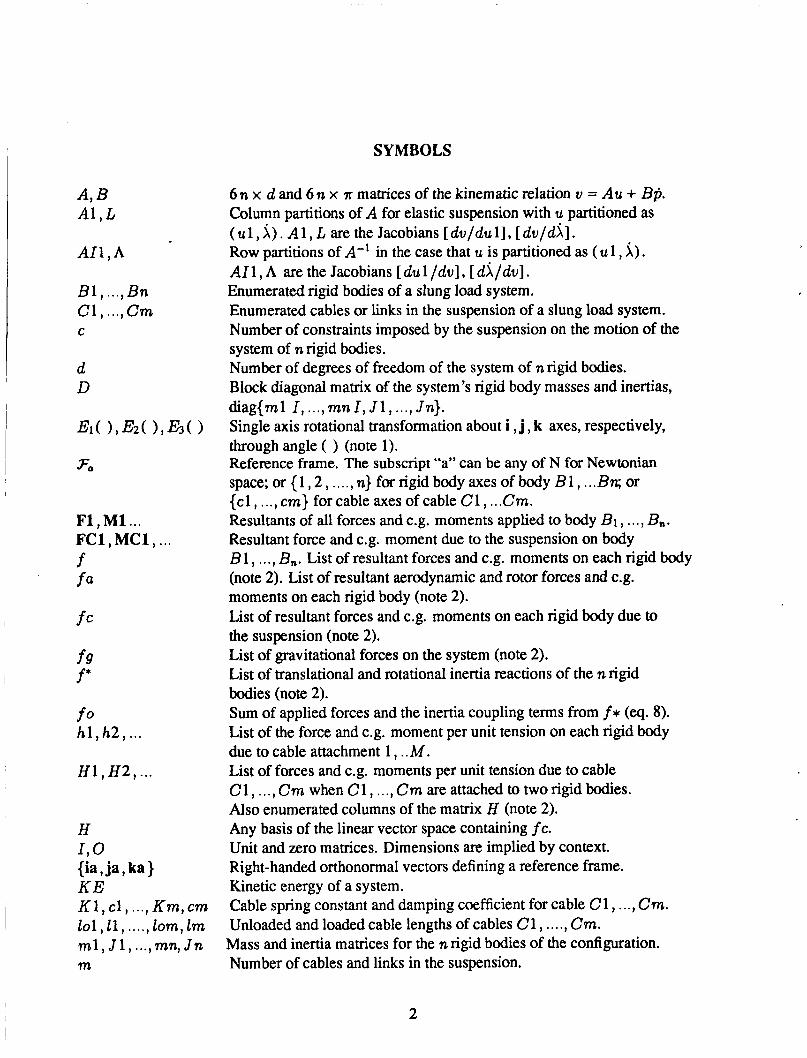
SYMBOLS

AI1,h

B1, ..., B n C1 , ..., Cm C

d D

F1, M1 .. . FC1 , MC1 , ... f fa

f c

f9 f*

fo h l , h2 , ...

H1 , H2 , ...

H L O {ia,ja, ka} K E K l , c l , ..., Km,cm l o l , l l , ...., lom,lm m l , J 1 , ..., mn, Jn m

6 n x d and 6 n x r matrices of the kinematic relation v = Au + Bp. Column partitions of A for elastic suspension with u partitioned as (u1,A). A l , L are the Jacobians [du/dul], [duldh]. Row partitions of A-’ in the case that u is partitioned as ( u l , i) . A I 1 , A are the Jacobians [ du 1 / d u ] , [ dh/du]. Enumerated rigid bodies of a slung load system. Enumerated cables or links in the suspension of a slung load system. Number of constraints imposed by the suspension on the motion of the system of n rigid bodies. Number of degrees of freedom of the system of n rigid bodies. Block diagonal matrix of the system’s rigid body masses and inertias, diag{ml I, ..., mn I, Jl , ..., Jn}. Single axis rotational transformation about i , j , k axes, respectively, through angle ( ) (note 1). Reference frame. The subscript “a” can be any of N for Newtonian space; or (1 , 2 , ...., n} for rigid body axes of body B1, ... Bn; or {cl , ..., cm} for cable axes of cable C1, ... Cm. Resultants of all forces and c.g. moments applied to body B1 , . . . , B,. Resultant force and c.g. moment due to the suspension on body B1, ..., B,. List of resultant forces and c.g. moments on each rigid body (note 2). List of resultant aerodynamic and rotor forces and c.g. moments on each rigid body (note 2). List of resultant forces and c.g. moments on each rigid body due to the suspension (note 2). List of gravitational forces on the system (note 2). List of translational and rotational inertia reactions of the n rigid bodies (note 2). Sum of applied forces and the inertia coupling terms from f * (eq. 8). List of the force and c.g. moment per unit tension on each rigid body due to cable attachment 1 , . .M. List of forces and c.g. moments per unit tension due to cable C1 , ..., Cm when C1, ..., Cm are attached to two rigid bodies. Also enumerated columns of the matrix H (note 2). Any basis of the linear vector space containing f c. Unit and zero matrices. Dimensions are implied by context. Right-handed orthonormal vectors defining a reference frame. Kinetic energy of a system. Cable spring constant and damping coefficient for cable C 1 , . . . Unloaded and loaded cable lengths of cables C 1 , . . . . , Cm.

Cm.

Mass and inertia matrices for the n rigid bodies of the configuration. Number of cables and links in the suspension.

2

M n P , 7r

Number of attachments of a cable to a rigid body of the system. Number of rigid bodies in the system. Suspension parameters which can be controlled, if any. p = ( pl , . . . , p w ) , where 7r is the number of such parameters. Generalized position coordinates of the system of n rigid bodies. q = (q1 , ..., q J T . Also any set of position coordinates of interest. Configuration position and velocity, given as a list of the inertial c.g. position and euler attitude angles, and the inertial c.g. velocities and angular velocities of the n rigid bodies. The physical vectors are given by their coordinates in standard axes (note 2). Position, velocity vectors relative to inertial space. Appended numbers indicate specific point or line segment. Skew-symmetric mamx representing cross product operation with V for vectors referred to Fa (note 1). Interaction force parameters for inelastic suspensions. s = ( s 1 , . .sc) Cable tensions for cable C 1 , . . , Cm. Transformation of physical vectors from frame & to frame .Fa.

All transformations are defined from Euler angles (note 1). Generalized velocity coordinates of the system of rigid bodies. Generalized velocity coordinates u for the system with elastic suspension composed of 6 n - c coordinates, u 1, of the system with inelastic suspension and c coordinates, i, which define the system motion due to suspension stretching. Configuration vector of inertia coupling terms in f* (note 2). Rigid body Euler angle triplet ( r ) , O , $) defining its attitude relative to inertial space, and angular velocity relative to inertial space. Appended numbers indicate specific body (note 1). Physical vector given by its coordinates in frame Fa (note 3). The subscipt “a” can be any of N for Newtonian space; or { 1 ,2 , . . . , n} for rigid body axes of bodies B 1 , . . . , Bn; or { cl , c2 , . . . , cm} for cable axes of cable C1, ..., Cm. Transpose of ( ) . Quantity associated with c.g. of a rigid body. Center of gravity. Degree of freedom. Equation of motion. Dot and cross product operators for physical vectors.

T

R,V

S( Va)

S

TC1, ... TCm Ta,b

U

( u l , i)

Notes: 1. Euler angles, single-axis rotation matrices, Euler angle transformations, and skew- symmetric matrices have the standard definitions found in aeronautical texts [ 13. Useful formulas are listed in the appendix to this report.

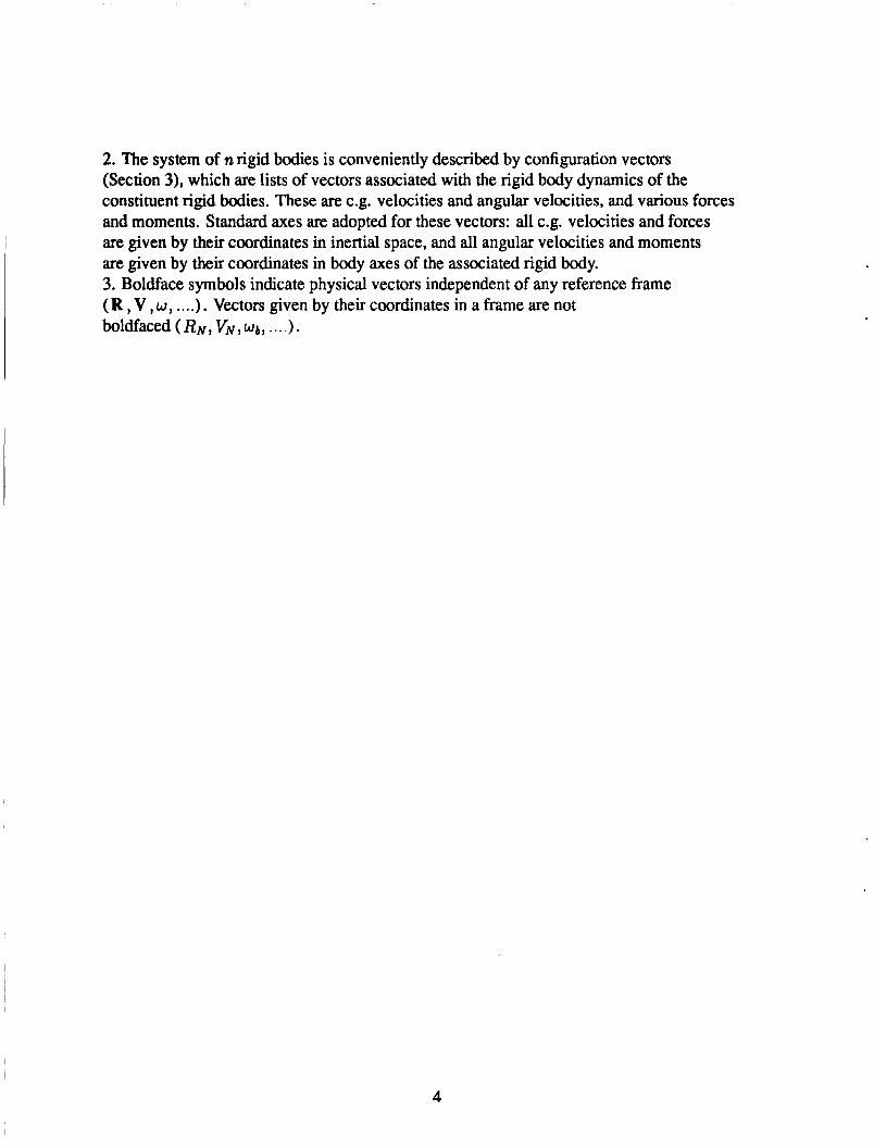
2. The system of nrigid bodies is conveniently described by configuration vectors (Section 3), which are lists of vectors associated with the rigid body dynamics of the constituent rigid bodies. These are c.g. velocities and angular velocities, and various forces and moments. Standard axes are adopted for these vectors: all c.g. velocities and forces are given by their coordinates in inertial space, and all angular velocities and moments are given by their coordinates in body axes of the associated rigid body. 3. Boldface symbols indicate physical vectors independent of any reference frame (R , V , w , . ...). Vectors given by their coordinates in a frame are not boldfaced (RN, VN, wb, .... ).

4

1. INTRODUCTION

1.1 Problem Background

Various actual and proposed slung load systems are illustrated in figure 1. Single helicopter slung load operations have been common since the 1950s. Such operations received extensive field use and development during the Vietnam war, and later research during the 1965-1975 period for the Heavy Lift Helicopter was focussed on the design of suspensions for stabilization of difficult loads, such as the standard 8x8x2O-ft cargo container (MILVAN).

The use of two or more helicopters has been periodically proposed since the early success of single helicopter operations, using suspensions consisting of cables and spreader bars as in figure 1 ([1],[2],[3]). Dual lift has received limited flight test, has been used to carry payloads in a few isolated commercial operations, and has been advocated as an alternative to developing larger helicopters with payloads ex- ceeding those of current helicopters [5] or to arranging for larger capacity helicopters than those available in a given situation. A significant obstacle to further operational development is the complexity of system motion and its coordination and stabilization along any typical maneuvering flight path [6], as well as for precision hover [7],[8]. Progress has been hampered by lack of realistic and comprehensive equations of motion for use in theoretical and simulation studies of these difficulties. Tractability of the equations for analysis and programming, and computational efficiency, are critical factors of interest, particularly for control designs using recent techniques based on inversion of the simulation model [9]. While the slung load systems can be viewed simply as a few rigid bodies connected by cables, considerable complexity arises in applying the classical methods used in the previous slung load literature to the multilift systems when the cables are modeled as inelastic. The approach taken in this papeir is to develop a systematic analytical formulation for general slung load systems, and to use the natural vectors and matrices of rigid body mechanics systematically in the applications work. The method is readily applied to the multilift systems and yields tractable, computationally efficient equations for the system dynamics. An alternate approach which avoids analysis is to consider use of one of the commercially available computer programs for the dynamics of general multibody systems. A third approach is to apply the previous derivation tech- niques to the multilift systems using symbolic digital computations to circumvent the excessive labor and inadequate error probabilities of extended hand analysis and programming. These alternate approaches, however, accommodate larger classes of dynamic systems and do not obtain the advances in tractability and computational efficiency achieved here by specializing to the smaller class of slung load systems.

1.2 Equations of Motion for Slung Load Systems

The slung load systems of figure 1 are viewed here as members of a class of systems consisting of rigid bodies connected by massless straight-line links which can be elastic or inelastic, and which support only forces along the link. These systems are characterized by the mass and inertia parameters of the rigid bodies and the suspension’s attachment point locations, unloaded link lengths, and link elastic parameters. Simulation equations are derived below for the entire class.

The limitations of these class properties in representing the slung load systems are as follows. First, the bodies are assumed to be rigid; this assumption excludes from consideration elastic helicopter and rotor

5

(3)

n = # RIGID BODIES

c = #CONSTRAINTS (INELASTIC SUSPENSION) d = 6n-c = # DEGREES OF FREEDOM

m = # OF CABLES

SYSTEM n c d m 1 2 1 1 1 1 2 2 2 1 0 2 3 2 3 9 4 4 2 3 9 3

5 3 2 1 6 2 6 4 4 2 0 4 7 3 2 1 6 2

8 5 6 2 4 6

Figure 1.- Examples of slung load systems.

6

modes, and non-rigid loads such as half-filled tanks of liquid and long, very flexible loads. Second, cable mass and aerodynamics are neglected, and cable stretching is neglected in the inelastic cable model case. These class properties are expected to suffice for realistic representation of the low bandwidth regime of interest in trajectory control studies.

Previous derivations of the equations of motion (EOMs) for single helicopter slung load analysis and simulation have assumed either inelastic cables ([lO],[ll],[12],[13]), or elastic cables ([14],[15],[16]), or accommodated both cable models, [ 171. Previous work on the EOMs for the multilift systems has yielded limited results. In [ 181 a general formulation for these systems is given, where: the bodies are assumed to be point masses and the cables inelastic, and [ 191 contains equations for the same approximation of the three-body dual lift system 7 of figure 1. In [7],[8] linearized equations for hover are given for the four- body dual lift system 6 of figure 1, assuming inelastic cables and a point mass load. Most of the previous work is specialized to particular suspension geometries. Exceptions are [14],[16] which account for the set of elastic suspensions in which all cables connect two bodies.

The equations have been derived in the above-cited works from Lagrange’s equation for general dy- namic systems or from the Newton-Euler equations for rigid body motion. For elastic cables, the Newton- Euler equations are readily applied to all suspensions in which all cables can be considered to connect two bodies; this includes the multilift systems. However, in practice, cables are relatively stiff so that the rigid body motion with inelastic cables differs very little from that with elastic cables, and a reduced order, inelastic cable model is of interest in trajectory control analysis. EOMs for inelastic cables have usually been derived from Lagrange’s equation since the nonworking constraint forces are systematically elimi- nated, equations are given for a minimal set of generalized position coordinates and usually contain lengthy quadratic dynamic terms. In view of these factors, nearly all control analyses utilize linearized EOMs for inelastic cables, while simulations have been implemented for both elastic cablles (e.g., [14],[15]) and in- elastic cables with linearized dynamics for the load-suspension motion [ 131.

The equations for inelastic cables differ considerably from those of elastic cables in form, and in an- alytical and computational requirements. This difference becomes acute for dual lift. The elimination of constraint forces in the inelastic cable derivation requires the inversion of a d x d system matrix for which an analytical inverse is unknown (d is the number of degrees of freedom; d = 20 for the dual lift system 6 of fig. 1). The inversion requires an analysis of the matrix conditioning over the flight envelope of interest and the identification of appropriate inversion algorithms. Together with the evaluation of the large num- ber of quadratic dynamic terms, much more computation is required than for the elastic cable model. In addition, physical insight is obstructed by this matrix in the inelastic cable model, whereas the elastic ca- ble representation can be fully expanded in terms of the familiar vectors and matrices of three-dimensional rigid body mechanics.

In the present work, simulation equations are derived by applying the Newton-Euler equations to each rigid body, defining configuration vectors, introducing generalized velocity coordinates, and apply- ing D’Alembert’s principle to the configuration of rigid bodies. This approach is similar to that taken in [20],[21],[22] for general multibody systems. General equations are obtained for the class of slung load systems, including elastic or inelastic cables, and any set of generalized coordinates. Three formulations are derived. The first two generalize the previous case-specific results in the slung load literature for elas- tic and inelastic cables. The third is a new formulation for inelastic cables obtained by appropriate choice of the generalized coordinates in the elastic cable formulation; that is, they are chosen to partition into d coordinates representing the configuration motion with inelastic cables, and c coordinates which define the

7

configuration motion due to cable stretching, where c is the number of constraints imposed by inelastic

coordinates. The result for inelastic cables is that the constraint forces are explicitly determined and ap- pear as an additive term in the equations of motion as in the elastic cable equations. This form requires the inversion of a much smaller c x c matrix (c = 4 for system 6 of fig. l), which occurs only in the additive constraint force term.

The third formulation has reduced computational penalty relative to the elastic cable equations, can be integrated with the elastic cable equations in one simulation, and can be expanded nearly completely in terms of natural vectors and matrices. It is readily applied to the multilift systems, and equations are given for the dual lift system 6 of figure 1. The three-body dual lift systems 5 and 7 of figure 1 are subsystems of the 4-body system 6, and these are readily given as specializations of the results for system 6 and integrated into the same simulation. The derivation and results are sufficiently brief for hand analysis and computer programming to be practical.

In these results, the equations are given in terms of natural vectors and matrices with reference frames indicated. The generalized coordinates are comprised of natural vectors and this can be done in most ap- plications owing to the method of selecting these coordinates to represent an unconstrained system (elastic cables) with a constrained subsystem (inelastic cables). The dynamic terms can be represented entirely as

This provides a programmable form of acceptable brevity and easy physical insight. It permits analysis and programming in terms of these three-dimensional vectors and matrices, and allows the devices of efficient coding to be applied to the vector-mechanical structure of the equations prior to treating the mass of scalar terms. Further expansion to scalars, if desired, is not obstructed.

I cables. This usually can be done by including appropriate cable velocity coordinates in the generalized

I coordinate transformations, and cross products arising from Coriolis and centripetal effects and moments.

1.3 Equations of Motion for Multibody Systems

A large body of literature on the dynamics of multibody systems has accumulated since the early 1960s in response to requirements in the design of machines, spacecraft, robotic arms, human motion models, etc., and the relevance of its formulations and results to multilift systems is of interest. The principal aim in this literature has been the development of general purpose computer programs to provide equations of motion from a minimal amount of user input data to define the multibody system. This is motivated by the impracticality or excessive labor of hand derivation in most working circumstances in these applications. Theory and analysis are given, for example, in [22],[23],[24], and surveys of computer programs which are equations of motion for a general system or which generate and compile symbolic case-specific code from user inputs are found in [25],[26]. Slung load systems differ from these applications. First, slung load systems with inelastic cables have only a few constraints compared to the number of degrees of freedom (DOFs) and can equally well be represented as unconstrained. The applications cited above are all highly constrained with only a few degrees of the freedom; e.g., spacecraft and robotic arms are commonly rep- resented as nrigid bodies with fixed orbit or base connected by n - 1 joints which permit one degree of freedom of relative motion, hence there are n + 2 DOFs. Consequently, a formulation in which a d x d matrix is formed and inverted is computationally more efficient for these applications compared to one con- taining a c x c matrix, while the converse is true for slung loads. Secondly, the interbody connections are modeled as joints in nearly all of this literature and often the generalized coordinates are predefined based

8

on the joint model. These features are advantageous for the applications cited above but their adaptation to cable-connected bodies is unclear.

One code-generating program, NEWEUL, and its underlying formulation given in [20],[21],[22] avoids these specializations and can be applied to slung loads. The equations from this program are in the conventional form requiring the inverse of a d x d matrix, and can be used where this formulation is satisfactory. An alternate computer-based approach is to utilize symbolic computations to carry out rou- tine analytical steps, such as the derivatives in Lagrange’s equation and routine code optimization. The general possibilities of applying MACSYMA [27] for this are discussed in [28] and the approach is used in [8] to derive linearized hover equations for the dual lift system 6 of figure 1 from Lagrange’s equation. In general, these computer-generated codes are fully expanded to scalar components and the resulting pages of expressions are unsuited to hand analysis or physical insight in larger problems, but substantial advantages are obtained where this is not a consideration.

For slung loads, the present paper provides a method which makes hand derivation, analysis, and pro- gramming feasible for the dual lift and multilift systems, and a new form of the equations which improves computational efficiency of the inelastic suspension case over previous forms. Results are given for the dual lift systems. A further technical paper is in progress which expands the present material to include EOMs for additional slung load systems in figure 1, EOMs for degenerate btdy (point mass, rigid rod) approximations, and linearized EOMs both for general slung load systems at general reference flight con- ditions and for the dual lift system with spreader bar.

2. SYSTEM DESCRIPTION

The systems of interest consist of one or more helicopters which support a load (more than one load in some instances) by means of a suspension. The load to be supported by the helicopters due to gravity, load acceleration, and aerodynamics is dominated by gravity for typical slung loads and nominal trajectories. The suspension can include spreader bars of non-negligible weight (e.g., the multilift systems) and other- wise consists of straight line links made up of cables, usually of nylon webbing, along with hooks, rings, bars, isolator springs, or other hardware [29]. Suspension designs with controllable geometry obtained by active cable winching and attachment point movement have been proposed for load attitude stabilization in [30],[31], and are included in the present formulation.

These systems contain n rigid bodies, B 1 , . .. . Bn (helicopters, load, spreader bars). The remainder of such a system (termed the suspension hereafter) consists of m straight-line links which support only force in the direction of the link (only tension in the case of cables), and has negligible mass and aerodynamic force compared to those of interest in trajectory control. Every link is connected at both ends to a rigid body or to another link. The links can be modeled as inelastic, in which case c 5 m holonomic (position) constraints are imposed on the motion of the rigid bodies, and the system has d = 6 n - c degrees of freedom. Values of c, d are listed in figure 1 for the systems shown there. For example, in system 3 of figure 1 the load and 4 inelastic cables form a single rigid body with a point held fixed to the helicopter, so that c = 3 . In classical mechanics, the motion of such a system is usually represented by d EOMs for d independent accelerations with the nonworking constraint forces systematically eliminated. Additionally, equations for a minimal (d) or nonminimal set of motion variables can be given with the constraint forces present, but expressed in terms of the applied forces and states. Alternatively, the links can be modeled as elastic due to cable or isolator spring stretching, in which case there are 6 n DOFs and the corresponding

9

6 n EOMs require calculation of the forces applied by the suspension to the bodies from the suspension stretching and cable elasticity parameters.

An examination of cable and suspension elasticity and its effect on rigid body motion is found in [32]. Cable stretching under tension is usually modeled as that of an undamped spring with damping supplied by the aerodynamic resistence of the attached bodies. Cables tend to be stiff, but the suspension design must avoid an upper bound given by resonance with the helicopter rotor frequency (around 4-5 hz), where a divergent pilot-induced oscillation vertical bounce mode has been observed near hover. The net result is natural frequencies of practical suspension links around 2.0 - 2.5 hz. This frequency is sufficiently high to be disjoint from the frequency range of interest in trajectory control (around 0.25 hz). The correspond- ing mode is one of rapid and significant cable tension variations, but with small stretching excursions so that the rigid body coordinates are almost unaffected [16]. Both elastic and inelastic suspension models are of interest in trajectory control. For practical suspensions, simulations can employ the simpler, more computationally efficient nonlinear equations of the elastic model. If suspension stiffness were signifi- cantly greater, then difficulties of numerical stability and ill-conditioning would arise in real-time digital simulation of the higher frequency, lower amplitude cable stretching motion. In control designs, practical suspensions are approximated as inelastic to eliminate feedback of states with negligible influence on the rigid body motion. If suspension stiffness were significantly lower, then the lower frequency, higher am- plitude motions due to cable stretching would be of interest in trajectory control. The present report studies simulation equations for both elastic and inelastic suspensions.

The simulation of cable collapse is an application detail outside the present scope. If a cable collapses, the resulting system is still a member of the class and can be simulated. However, practical suspensions are designed and operated such that cable collapse does not occur except during large unstable excursions from the nominal configuration, or a redundant cable can collapse under ordinary motions but leaves the constraints imposed by the suspension invariant.

3. EQUATIONS OF MOTION OF GENERAL SLUNG LOAD SYSTEMS

3.1 Configuration Vectors

Physical vectors are referred to inertial or body axes reference frames in the following. Translational motion and forces are given in inertial coordinates, and rotational motion and moments in body axes. The reference frame is indicated by a subscript, which is N for inertial space and i E { 1,2, ...., n} for body axes of the ith body. Body axes components of translational velocity and motion variables relative to a reference body are commonly used in slung load simulations, and are readily introduced later when selecting generalized coordinates for an application.

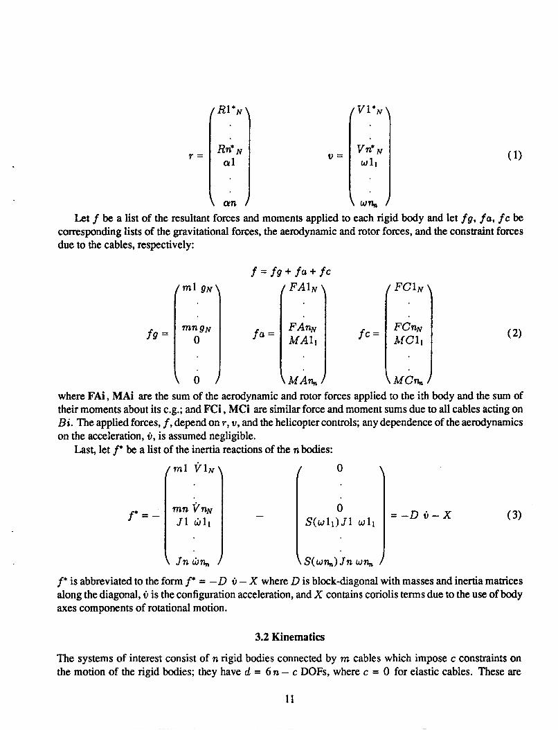
It is convenient to use configuration vectors which define the motion and forces of the nrigid bodies, whose masses, inertias, c.g. translational motion, Euler attitude angle triplets, and angular velocities rela- tive to inertial space are denoted by ( rn 1 , J 1 , R1*, V1* , a 1 , w 1 ) , . . . , ( mn, Jn, Rn *, Vn * , an, wn ) . The configuration vectors of position, r, and velocity, u, are defined as lists of the rigid body c.g. positions and Euler attitude angles, and the rigid body cog. translational and angular velocities:

10

?-= V =

Let f be a list of the resultant forces and moments applied to each rigid body and let f g , fa, f c be corresponding lists of the gravitational forces, the aerodynamic and rotor forces, and the constraint forces due to the cables, respectively:

f = f g + fa + f c

where FAi , MAi are the sum of the aerodynamic and rotor forces applied to the ith body and the sum of their moments about its c.g.; and FCi , MCi are similar force and moment sums due to all cables acting on Bi. The applied forces, f, depend on r , v , and the helicopter controls; any dependence of the aerodynamics on the acceleration, 8, is assumed negligible.

Last, let be a list of the inertia reactions of the n bodies:

mn J 1

f*=-

\ Jn

0

S ( w h ) Jn wn,, ,

f* is abbreviated to the form f’ = -D u - X where D is block-diagonal with masses and inertia matrices along the diagonal, ir is the configuration acceleration, and X contains Coriolis terms due to the use of body axes components of rotational motion.

3.2 Kinematics

The systems of interest consist of n rigid bodies connected by m cables which impose c constraints on the motion of the rigid bodies; they have d = 6 n - c DOFs, where c = 0 for elastic cables. These are

1 1

holonomic systems; that is, the constraints imposed by an inelastic suspension can be given as functions of position only. These constraints are usually time-invariant, but in the special case of active cable winching

controllable geometric parameters of such a suspension, p = ( pl , . . . , p W ) = , are included in the development below.

For holonomic systems with d DOFs there exist d generalized position coordinates, q = ( q1, ... , q d ) T , which suffice to locate all points in the system and also the configuration position:

l or attachment point movement these have explicit dependence on time. To accommodate this case, the

r = r ( q , p ) ( 4)

and d generalized velocity coordinates which suffice to define all inertial velocities of the system:

= U ( q , p ) Q ( 5 )

I The configuration velocity is related to u by a linear expression of the form:

I Here, U is a nonsingular d x d matrix; it can be unity, but velocity coordinates different than q are commonly useful in applications. Note that v is asserted in equation (6) to be linear in u, p . This follows from the usual linear relationship u( i ) from rigid body kinematics (appendix)

a = 1, ..., n vi; = Ai;

W i i = W ( a i ) &i

and equations (4) and (5). A is a 6 n x d matrix. For inelastic suspensions, A expresses the constraints by confining that part of the configuration velocity due to u to the d-dimensional linear vector subspace defined by the columns of A. If f i = 0 then this subspace is tangent to the configuration trajectory, r( t ) .

I 3.3 Equations of Motion from D'Alembert's Principle

D'Alembert's principle applied to a rigid body, Bi, of a holonomic system yields the following equations for the inertial motion (e.g., see [33]):

[ M i ; - J i Lji; - S ( ~ i i ) J i wi;lTdaii = 0

where Fi , Mi are the total applied forces and moments about the c.g. of body Bi, and dRi *, d ai are the c.g. position and rigid body attitude changes due to any perturbation of the generalized coordinates, dq, or equivalently, due to any small motion, udt:

12

The velocity Jacobians [ dVi*,/du] and [ dwii/du] are the appropriate rows ,of A in equation (6) and the result is valid for arbitrary u. The same result for all nrigid bodies of a slung load system can be combined to get the following d equations of motion:

A T ( f + f * ) = O ( 7)

This result can be obtained almost as easily from Kane's equations [33], since ATf and ATf* can be recognized as lists of the generalized active and inertia forces for each DOFI Lagrange's equations have been used in much of the previous literature on slung load systems with inelastic suspensions, and can be applied to the general slung load system where kinetic energy is the sum of the kinetic energies of the constituent bodies:

T T T T 1 1 2 K E = - u T D u = T ( Q ~ [ U ~ A ~ D A U ] ~ + ~ Q ~ [ U A D B ] @ + @ B DBP)

For holonomic systems, ATf and ATf* are equal to lists of the generalized applied and conservative forces, and the derivatives of the kinetic energy [33], respectively, in Lagrange's equations. D'Alembert's principle is used here for slung loads in order to maintain contact with the underlying rigid body dynamics. One consequence is the compact, well-structured formulation of the second-order velocity dynamics in terms of the rigid body velocities, u, seen in X (eq. 3) and in the remaining such terms in the dual lift example given later. Lagrange's equations lose contact with u in KE and generate the second-order velocity dynamics in terms of the generalized velocity coordinates, q, from derivatives of KE. The result is a large number of scalar terms with no apparent structure, and the number of such terms grows rapidly with the number of rigid bodies.

To obtain the simulation equations, differentiate equation (6) with respect to time, introduce this in f* (eq. 3) , and solve equation (7) for u:

( 8) u = [ATDA]-'AT[ f o + f c ]

where A

f o = f g + f a - D A u - X - D ( B p + B I j ) The configuration vector f o denotes the combined external forces, second-order velocity effects due to the choice of coordinates u, u, and the inertia reaction of the configuration to p( t ) .

If the cables are elastic, then A is a nonsingular 6 n x 6 n matrix and:

u = A-'D-'[ fo + f c ] ( 9)

In the case that p = 0 and we choose u = u, then A = I and the result is identical to the Newton-Euler equations applied to each body:

This result can be given by inspection of the system and has been the starting point in most work which as- sumes elastic cables. Equation (9) generalizes this to allow any choice of generalized velocity coordinates; for example the use of cable velocity coordinates in u provides a convenient and well-conditioned calcu- lation of cable lengths and directions for use in the calculation of the cable forces, fc. It is remarked here that the matrix A-I in equation (9) represents the kinematic relation u( u ) and can be given analyticaIIy

V = P [ f g + f u - X + f c ]

13

from the kinematics as readily as the matrix A representing the reverse relation v( u) . It is unnecessary to perform matrix inversion to obtain A-' .

The constraint force, fc , in equation (9) can be given as a sum of forces and moments applied by the suspension at each attachment point:

M f c = h j TCj

j = 1

where j enumerates every attachment of a cable to a rigid body, hj is a configuration vector defined in the next section, and TCj is the cable tension which is given by the spring model of the cable as

T C ~ = m a z { ~ , K j ( t j - t o j ) + c j ioj) j = 1 , 2 , .... , M

where { to j , Kj, c j ) are the unloaded cable length, and cable spring and damping constants. Cable damp- ing, c j # 0, is introduced in [16] but otherwise this has been neglected in simulations with elastic cable models. The spring constants K, care related to the natural mode parameters by w: = K/m, 25w, = c/m,

tension and stretch can be calculated in cases with nonredundant suspensions from the solution for the constraint forces, fc, for inelastic cables given below. Alternatively, the configuration can be allowed to settle from an approximate initial arrangement, possibly with the aid of cable damping as a settling device.

I where rn is the load mass supported by the cable. In simulations with elastic cables, initial values of cable

3.4 Equations of Motion for Inelastic Suspension: Method 1

If the cables are inelastic then the constraint forces, fc, drop out of equation (8). This result is shown as follows. First, enumerate the cable attachments 1,2, ..., M at attachment points R l , R2 , ..., R M on their corresponding bodies Bi( 1) , Bi( 2), . .. , Bi( M ) . One or more cables are attached at an attachment point and every such attachment of a cable to a body is numbered. The constraint force on the configuration is then (see fig. 2):

M f c = chj TCj

j = 1

where T C j is the cable tension. The j th cable attachment at point Rj on body i ( j ) applies a force and moment to Bi( j ) given by:

FCij = kcj TCj

MCij = (Ri*j x kcj) TCj

where kcj is the cable direction outward from the body and RC *j is the attachment point to c.g. moment arm ( Rj - ki *) . Thus, h j in equation (10) is a configuration vector whose nonzero elements are kcj and (Ri *j x kcj) , corresponding to the constraint force and moment on B i ( j ) due to thej th cable attachment, per unit tension.

Second, enumerate the cables and links which constitute the suspension, C1, C2, ..., Cm. Each end of a cable or link is attached to either a rigid body or to another link. In the special case that all cables are attached at both ends to rigid bodies then all terms in equation (10) can be combined in pairs, with each pair corresponding to a single cable:

14

\ Bi

i;"

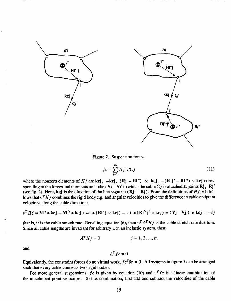
Figure 2.- Suspension forces.

m

f c = H j T C j j = 1

where the nonzero elements of H j are kcj , -kcj , (Rj - Ri *) x kcj , -( R j' - Ri '*) x kcj corre- sponding to the forces and moments on bodies Bi, Bi' to which the cable Cj is attached at points Rj , Rj' (see fig. 2). Here, kcj is the direction of the line segment (Rj' - Rj) . From the definitions of Hj, u it fol- lows that u T H j combines the rigid body c.g. and angular velocities to give the difference in cable endpoint velocities along the cable direction:

wTHj = Vi * kcj - Vi'* kcj + wi ( Ri *j x kcj ) - wi ' ( Ri '*j' x kcj ) = ( Vj - Vj') 0 kcj = -dj

that is, it is the cable stretch rate. Recalling equation (6), then u T A T H j is the cable stretch rate due to u. Since all cable lengths are invariant for arbitrary u in an inelastic system, then:

*.

A T H j = 0 j = 1 , 2 , ..., m

and A T f c = 0

Equivalently, the constraint forces do no virtual work, f?6r = 0. All systems in figure 1 can be arranged such that every cable connects two rigid bodies.

For more general suspensions, fc is given by equation (10) and wTfc is a linear combination of the attachment point velocities. To this combination, f i s t add and subtract the velocities of the cable

15

interconnection points in the cable directions, and then apply the force balance condition to the linear combinations of cable forces at these interconnections. The result is:

M m m

v T f c = z V j 0 kcj T C j = x ( V j - V j ’ ) 0 kcj T C j = - x & T C j ( 12) j = 1 j = l j = 1

where the second and third sums are taken over all cables and (t i} are cable lengths. Consequently, if the suspension is inelastic then all cable lengths are invariant for arbitrary u and:

ATfc = 0 (13)

Equation (8) for inelastic suspensions is now:

= [ATDA]-’ATfo

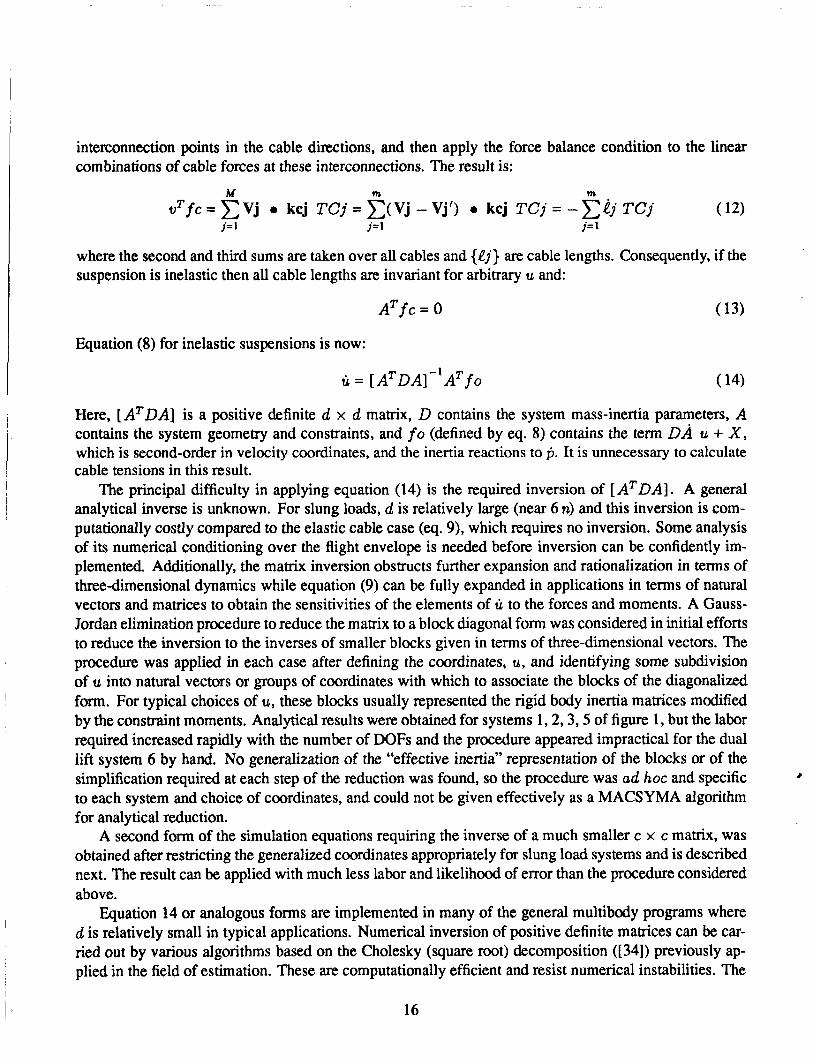
Here, [ATDA] is a positive definite d x d matrix, D contains the system mass-inertia parameters, A contains the system geometry and constraints, and fo (defined by eq. 8) contains the term D A u + X, which is second-order in velocity coordinates, and the inertia reactions to p . It is unnecessary to calculate cable tensions in this result.

The principal difficulty in applying equation (14) is the required inversion of [ ATDA]. A general analytical inverse is unknown. For slung loads, d is relatively large (near 6 n) and this inversion is com- putationally costly compared to the elastic cable case (eq. 9), which requires no inversion. Some analysis of its numerical conditioning over the flight envelope is needed before inversion can be confidently im- plemented. Additionally, the matrix inversion obstructs further expansion and rationalization in terms of three-dimensional dynamics while equation (9) can be fully expanded in applications in terms of natural vectors and matrices to obtain the sensitivities of the elements of u to the forces and moments. A Gauss- Jordan elimination procedure to reduce the matrix to a block diagonal form was considered in initial efforts to reduce the inversion to the inverses of smaller blocks given in terms of three-dimensional vectors. The procedure was applied in each case after defining the coordinates, u, and identifying some subdivision of u into natural vectors or groups of coordinates with which to associate the blocks of the diagonalized form. For typical choices of u, these blocks usually represented the rigid body inertia matrices modified by the constraint moments. Analytical results were obtained for systems 1 , 2 , 3 , 5 of figure 1, but the labor required increased rapidly with the number of DOFs and the procedure appeared impractical for the dual lift system 6 by hand. No generalization of the “effective inertia” representation of the blocks or of the

to each system and choice of coordinates, and could not be given effectively as a MACSYMA algorithm for analytical reduction.

A second form of the simulation equations requiring the inverse of a much smaller c x c matrix, was obtained after restricting the generalized coordinates appropriately for slung load systems and is described next. The result can be applied with much less labor and likelihood of error than the procedure considered above.

Equation 14 or analogous forms are implemented in many of the general multibody programs where d is relatively small in typical applications. Numerical inversion of positive definite matrices can be car- ried out by various algorithms based on the Cholesky (square root) decomposition ([34]) previously ap- plied in the field of estimation. These are computationally efficient and resist numerical instabilities. The

simplification required at each step of the reduction was found, so the procedure was ad hoc and specific &

16

*

conditioning of the coefficient matrix [ ATDA] depends on A in equation (14) or, equivalently, on the choice of coordinates, u. In the multibody programs these coordinates are often preselected based on the joint model of interbody connections, and these appropriate coordinates tend to result in well-conditioned coefficient matrices. In the present work, the interbody connections are suspensions comprised of cables; it is left to the applications phase to determine in each case what constraints are imposed and what choice of coordinates best represents the constrained system motion.

3.5 Equations of Motion for Inelastic Suspension: Method 2

The approach in this section is to select the generalized velocity coordinates for the elastic system in equation 9 so as to separate motion due to cable stretching from the remaining motion with invariant cable lengths, and then study the results when the stretching motion is nulled. A solution for the constraint force and new simulation equations for the inelastic system are obtained.

First, let the generalized velocity coordinates of the elastic system, u, be comprised of 6 n - c coor- dinates, u l , of the system with invariant cable lengths and c length rates, i, which suffice to define the motion due to cable stretching. In general, if the c independent position constraints imposed by an inelastic suspension are given by {A 1( r ) = 0 , ..., Xc( 7 ) = 0) then X can be taken as ( A 1, ..., A c ) ~ . For slung load systems, X can usually be taken as cable lengths and the complete set of coordinates ( u l , A) taken as the c.g. velocity of a reference body, the angular velocities of all rigid bodies, and. the cable angular velocities and stretching rates.

Next, substitute the partitioned u in equations (6) and (9):

v = A u + B p = A1 u l + L A + B p ( 15)

where fo is defined in equation (8); A1 , L are the 6 n- c and c columns of A which, respectively, define the contributions of u l , to v ; and AIIT, AT are the 6 n- c and c rows of A-' which respectively define the relations ul ( v ) and A( u ) . As noted earlier, A-' can be obtained without matrix inversion since it defines the relation u( v ) for the elastic system and can be given from the kinematics as readily as A, which defines the relation u( u) .

Equation (16) gives the simulation equation for systems with elastic suspensions in terms of the coordi- nates ( u 1 , A), where u 1 leaves the cable lengths invariant. The influence of cable stretching motion on u 1 can be viewed by entering the derivative of the partitioned generalized velocity coordinates equation (15) in f* and rederiving equation (8). The first 6 n - c equations can be arranged as

where fo is as defined with equation (8) except that A1 u l replaces A u. 14s in equation (14), fc drops out ( AIT fc = 0 in view of equation 13) and the result differs from the inelastic system equations (eq. 14) only in the presence of the configuration acceleration due to elastic stretching. The effect of the stretching motion on u l depends on the cable spring constants: for a fixed disturbance, the extremes of A decline with increasing spring stiffness, while the extremes of the term in 5 remain fixed in magnitude, but I( t) increases in frequency [16].

17

For inelastic suspensions, 1 = 0 and equation (16) gives c equations from which to calculate the constraint forces:

The constraint force can be given in terms of c independent parameters; that is, it can be given in the form: O=ATD- ' ( fo+ f c ) (17)

f c = [ H1, .."I [ ") = H s

sc

where s is arbitrary, ( H j ) are configuration vectors, and rank [ H I = c. From equation (13), AITH = 0, and from the construction of A-' , AITA = 0. Therefore, the columns of H and A are both bases of the same linear vector space, and A can be used to define the constraint force:

f c = A s (18)

where A is the Jacobian, [ d ) ; / d v ] , and s has units of force. Introduce equation (1 8) in equation (17) and solve for B:

8 = -[ATD-'A]-'ATD-I f o ( 19) Further, A can be replaced in equations (18, 19) by any other convenient basis, H, of the space containing f c. For example, in the special case that every cable connects two bodies and c = m, then s can be taken as the c cable tensions with the basis vectors, H 1 , . . . , Hc, as defined by equation (1 1) above.

The cable tensions are related to s, and can be uniquely determined from s if the suspension is not redundant. However, the constraint force applied to the configuration, f c, can always be calculated. A suspension can be separated into disjoint sets of interconnected links. Each such set imposes one holonomic constraint; if the number of sets is c then all cable tensions can be uniquely determined from s, but if it exceeds c then the constraints are redundantly imposed. In the special case that all cables connect two rigid bodies, then each cable is a disjoint set and all cable tensions can be found only if c = m.

Finally, the simulation equations are:

or, for the inelastic DOFs:

This result has several advantages over equation 14 for the slung load systems. First, the leading coefficient matrix, A l l , is known analytically. Second, equations (19), and (20) require the inversion of a c x c matrix, [ ATD- 'A] , where c = 1 for system 1 and c = 4 for the dual lift system 6, compared with the required inversion of an 11 x 11 and a 20 x 20 matrix, respectively, for these two systems when equation (14) is used. In many cases, the cable tensions can also be generated by equation (19).

Computational efficiency in calculating the dynamics can be compared by counting the number of multiplies required to generate ti, given A, A-' , D, D-' , f o . These are shown in table 1 for systems 1, and 6 of figure 1.

18

Table 1. Number of multiplies to calculate C

F I System 1 I System 6 I GeneralFormula I Eq. (9) Eq. (14) Eqs. (10-20)

60 264 6n(6n - i +2) 616 + g(112) 3430 + g(202) d((6n - i ) y + 12n +d) + g(d2) 119 868 + g(42) d(6n -i) + 3n(c2 + 9c + r) + c2 + g(c2)

Here, g() refers to the number of multiplies and divides required for the Cholesky inversion, which increases with the square of the matrix size ([34]). The general formulas (derivations omitted) include savings due to generic zeros, ones, and matrix symmetries. The number of coordinates u, v which is identical is represented by a in these formulas, and accounts for generic zeros and ones. In most cases, u can be selected such that a = 3n + 3. Additions are omitted from the operations count for brevity but this omission does not affect the conclusions. Equation (14) is representative of previous single-case formulations of the slung load dynamics with inelastic cables, as well as that in most of the multibody literature (e.g., [22]). As seen, equations (19) and (20) provide a significant reduction in the computational requirements to represent these dynamics, and the same conclusion applies to all systems of figure 1.

3.6 Procedure for Generating Simulation Equations

A procedure for applying and implementing the previous results is outlined in figure 3. Both equa- tion (16) for elastic suspensions and equations (19) and (20) for inelastic suspensions are included.

First, (figure 3a) analysis is required to determine c, define appropriate generalized velocity coordinates ( u 1 , A), and obtain expressions for A, A-' , A from the kinematics, and also expressions for B , B in the case that p f 0. Secondly, the simulation equations (16) or (19, 20) can be implemented as shown in figures 3b and 3c. For elastic cables, f c is obtained from ( h j , TCj ) which are defined with equations (10) and (1 1) above, and for inelastic cables, f c is obtained from equations (1 8) and (19). Subsequently, the rigid body kinematics v , r are obtained in the usual way or, more generally, this can be expanded to any set of velocity and position coordinates of interest, q , q after defining q( (I, 6) from the kinematics and geometry. For inelastic cables, the coordinates A and their equations can be eliminated, since A is theoretically zero. Alternately, all 6 nequations can be retained to permit simulation of both cable models; for inelastic cables, the computed 1 indicates numerical accuracy.

19

C

u l

i

U

number of holonomic constraints on configuration for inelastic suspension.

6n-c generalized velocity coordinates for system with inelastic suspension.

c generalized velocity coordinates defining suspension stretching motion.

6n generalized velocity coordinates for system with elastic suspension u=(ul*,P )*

A(r,p) the Jacobian [dv/du] obtained from the kinematics. A=[AlIL]

A-' (r,p) the Jacobian [du/dv] obtained from the kinematics.

B(r,p) the Jacobian [dv/dp] (Required only if p j 0).

(a) Quantities required a priori.

A-*=[AIlIA ]

fa = fa(r,v,6) (6 = helicopter controls)

fo = fg + fa- D A u - X - D(B p + Bp)

fc = { ci"fl h j rnaz(0, Kj ( t j - t o j ) }

sf

elastic cables -A[ATD-'A]-'ATD-' fo inelastic cables

= D-' (fo + fc)

u =A-' sf

u =Judt

v = A u + B p

i. = i.(v) or q = q(u,p)

r =J id torq=Jqdt

(b) Simulation equations.

,

Figure 3. Procedure for simulation of slung load systems

20

6

P-

P

. .e

~ ~

fo = f g + fa - X - D(& + & + BF)

~ ~~

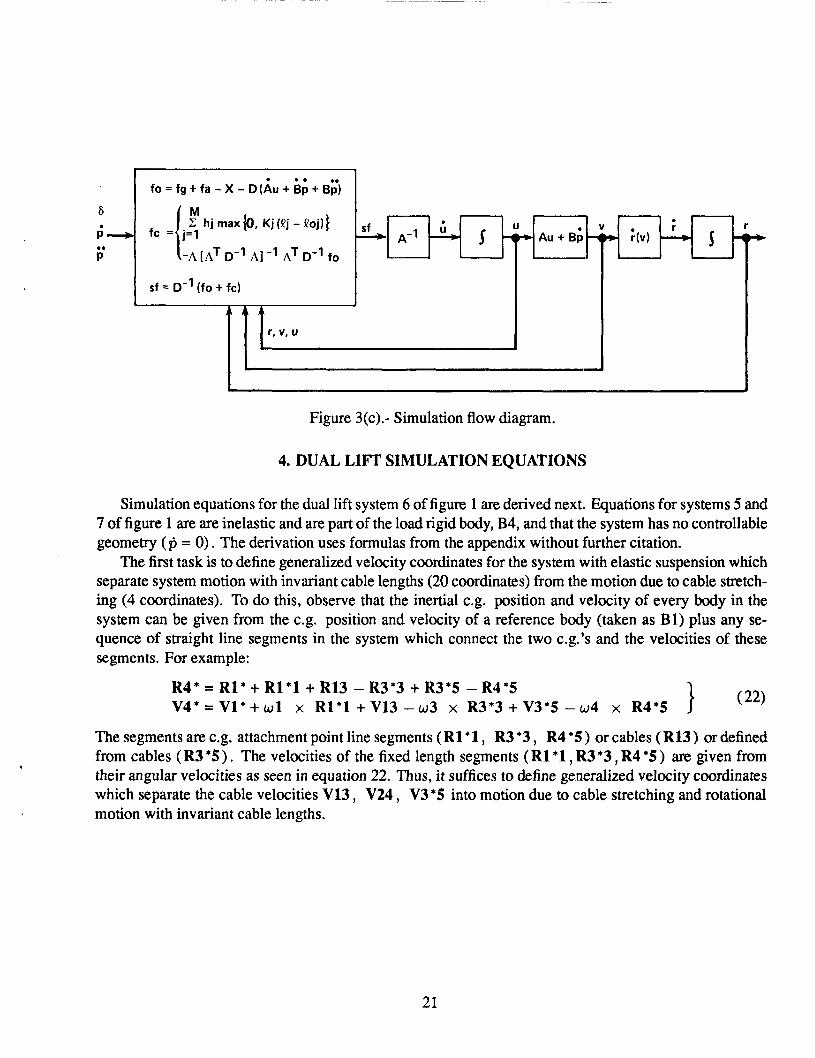
Figure 3(c).- Simulation flow diagram.

4. DUAL LIFT SIMULATION EQUATIONS

n

Simulation equations for the dual lift system 6 of figure 1 are derived next. Equations for systems 5 and 7 of figure 1 are are inelastic and are part of the load rigid body, B4, and that the system has no controllable geometry ( p = 0). The derivation uses formulas from the appendix without further citation.

The first task is to define generalized velocity coordinates for the system with elastic suspension which separate system motion with invariant cable lengths (20 coordinates) from the motion due to cable stretch- ing (4 coordinates). To do this, observe that the inertial c.g. position and velocity of every body in the system can be given from the c.g. position and velocity of a reference body (taken as Bl) plus any se- quence of straight line segments in the system which connect the two c.g.'s and the velocities of these segments. For example:

} (22) R4* = R1* + R l * l + R13 - R3*3 + R3*5 - R4*5 V4* = V1* + w l x R l * l + V13 - ~ 3 x R3*3 + V3*5 - w 4 x R4*5

The segments are c.g. attachment point line segments ( R l * l , R3 *3, R4 *S) or cables (R13) or defined from cables ( R3 5 ) . The velocities of the fixed length segments (R1*1 , R3 *3, R4 *5 ) are given from their angular velocities as seen in equation 22. Thus, it suffices to define generalized velocity coordinates which separate the cable velocities V13 , V24 , V3 *5 into motion due to cable stretching and rotational motion with invariant cable lengths.

21

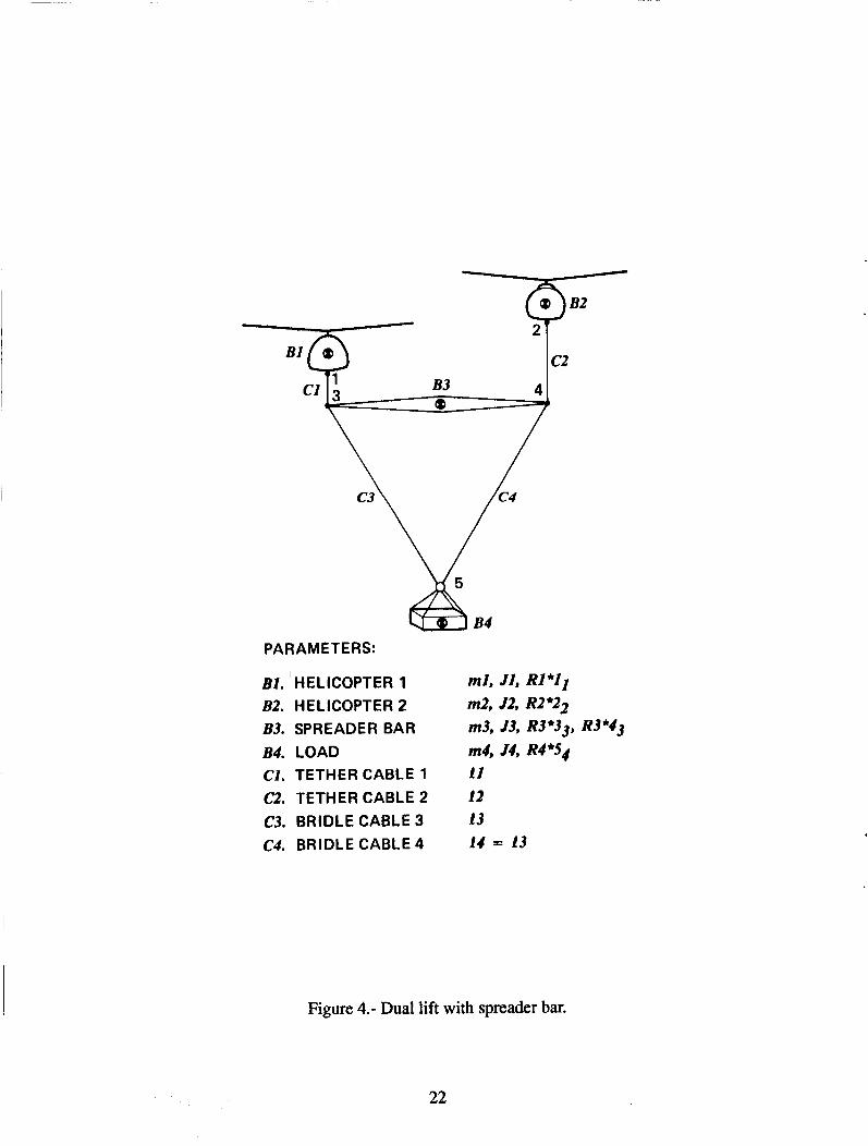
PARAMETERS:

BI . ' HELICOPTER 1 82. HELICOPTER 2 B3. SPREADER BAR B4. LOAD CI. TETHER CABLE 1 C2. TETHER CABLE 2 C3. BRIDLE CABLE 3 C4. BRIDLE CABLE 4

ml, J1, RI*l1 m2, J2, R2*22 m3, J3, R3*33, R3*43 m4, J4, R4*54 11 12 13 14 = 13

Figure 4.- Dual lift with spreader bar.

22

The tether cable velocities are treated as given in the equation table, table 2a. A cable axis, Fc, is defined for each cable with its IC-axis along the cable, and oriented inertially by pitch and roll angles from which the transformation to cable axes, Tc,N, is given. These angles are small when the cables are near the vertical. Expressions for the cable-axes components of the cable velocities V 13,1, V24,2 are given from derivatives of the appropriate position coordinates as shown, and are seen to be appropriate generalized velocity coordinates which separate rotational and stretching motion. Linear velocity components are used in preference to cable angle rates for simplicity in the relation v( u ) given later.

The velocity contributions of the bridle cables, C3, C4 are formulated in table 2b. These cables form a triangle with the spreader bar longitudinal axis, i3. Axes, Ft , are attached to the plane of the triangle. The triangle plane can have any roll angle, r j t , about i3, and R3'5 has components (423s, 4232) in this plane. To isolate the velocity coordinates ( &, d3 5, i!3 2) in an expression for V3 *5 define a reference frame, Fy, from the spreader bar Euler angles ( 63, $3) and then evaluate the inertial velocity of R3 *S as the sum of its velocity relative to F3!, denoted as VT , and the effect of the inertial rotation of 3 ' 3 1 , denoted as A VT . The three components of VTt are the desired generalized velocity coordinates. A, VT depends on the angular velocity of & I , which can be given from the spreader bar angular velocity as shown in table 2b.

Finally, the generalized coordinates, u, are assembled and related to the configuration velocity, v , by the matrix, A, given in table 2c. For simplicity of A, u contains as many of the rigid body velocities as possible, in addition to the required cable velocity coordinates. Here, u includes the c.g. velocity of a reference body, V l * N , and the angular velocities of all bodies. This can be done for most systems of figure 1 and the corresponding rows of A are from the unit matrix. The remaining rows generate v2*N, v3*N, V4 *N

from kinematic expressions analogous to equation (22) and contain only coordinate transformations and skew-symmetric matrices representing cross products with the c.g.-attachment point line segments in the coriolis velocity terms.

The rows of A-' which are not from the unit mamx generate the cable velocities, V 13 cl, V24 d, VTt , as differences of the attachment point velocities obtained from the rigid body velocities of the two bodies connected by the cable, and contain the same matrix objects found in the submatrices of A.

The configuration forces are assembled next. First, the applied forces and inertia coupling terms, fo, are assembled in table 2d as the sum of applied forces due to weight ( ml g , . . . , m4 g) , the forces and moments due to the aerodynamics and helicopter rotors ( FA1, . .. , MA4), and the inertia coupling term, X + D A u. The submatrices of A are defined in table 2c and their time derivatives are obtained principally from the derivatives of various coordinate transformations. A general formula for transformation rates is given in table 2d along with expressions for the cable axes angular velocities and the results for the terms from A u. These terms are seen to be principally coriolis and centrifugal accelerations and are compactlyexpressed in terms of the rigid body velocity coordinates. The time derivative of BT is obtained routinely, but it is omited from the equation summary for brevity. The vector elements off o are denoted F01, ..., M04 for brevity in the later equations.

23

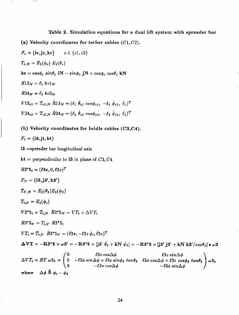
Table 2. Simulation equations for a dual lift system with spreader bar

(a) Velocity coordinates for tether cables (Cl, C2).

Fc = {ic, jc, kc} c E { c l , c 2 )

Tc,N = El(4c) E2(6c)

kc = COS^, sine, iN - sin+, jN + COS^, cosOC kN

R 1 3 ~ = e1 k r l N

R 2 4 ~ = 1, k C 2 ~

V13c1 = Tcl ,N A13N = (el dc1 cos$'cl, -11 d'cl, il)T V24c2 = Tc2,N R24N = (42 e c 2 cos4c2, -12 4 c 2 , i 2 ) T

(b) Velocity coordinates for bridle cables (C3,C4).

Ft = {i3,jt,kt}

i3 =spreader bar longitudinal ax is

kt = perpendicular to i3 in plane of C 3 , C 4

~ 3 ' 5 ~ = (e3a, 0, e3z)T

VTt = Tt,31 k3*531 = ( i 3 ~ , -e32 & , i 3 ~ ) ~

AVT = -R3*5 x w3' = -R3*5 x lj3' 4, + kN d 3 ] = -R3*5 x lj3'jS' + kN k3'/c0s6~] e w3

e32 c o s ~ 4 e32 s i n A 4 AVTt = BT w33 =

where

0

A4 !! dt - 4 3

-L3x s i n A 4 -+ l 3 2 sin43 tan63 L3x cosA4 + t 3 z C O S 4 3 tan93 (1 cos ~4 -132 s i n A 4

24

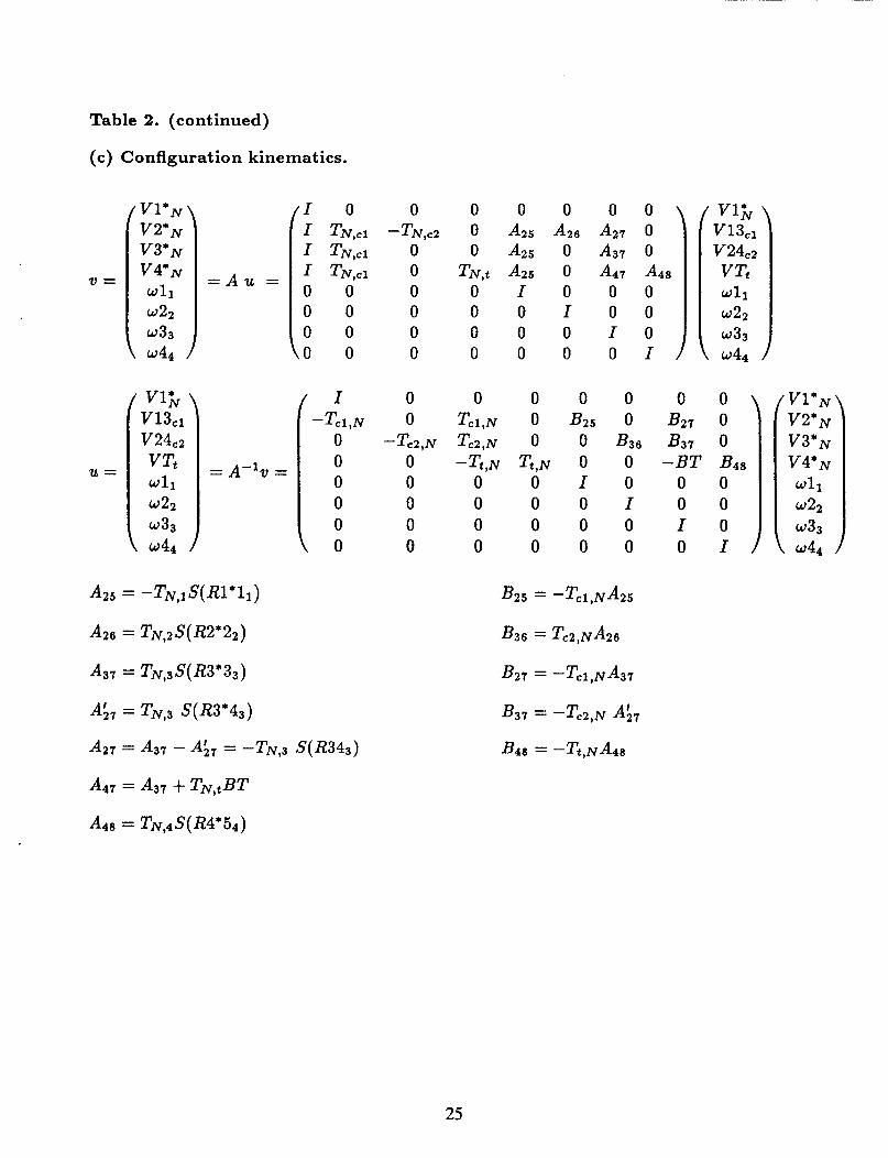
Table 2. (continued)

(c) Configuration kinematics.

V =

U =

/I 0 0 0 0 0 0 0 I TN,c l -TN,c2 0 A 2 5 A 2 6 A27 0 I TN,c l 0 0 A 2 5 0 A37 0 I TN,cl 0 T N , t A25 0 A47 A48 0 0 0 0 I O 0 0 0 0 0 0 0 I O 0 0 0 0 0 0 0 I O

t o 0 0 0 0 0 O I

I 0 0 0 0 -Tcl,N 0 T c l , N 0 B2

0 0 -Tt,N T t , N 0 0 0 0 0 I 0 0 0 0 0 0 0 0 0 0

, o 0 0 0 0

0 -Tc2,N Tc2,N 0 0

0 0 0

B36 B37 0 0 -BT B48

0 0 0 I 0 0 0 I O 0 O I

0 B27 0

25

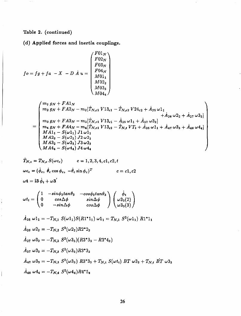
Table 2. (continued)

(d) Applied forces and inertia couplings,

M022

M 044

f o = f g + f a - X - D A ~ =

m3 m4

TN,c = TN,c s (wcc)

WC, = e, cos 4c, -8, sin+,)T c = cl,c2

w t = i3 it + w3'

c = 1,2,3,4, c l , c2, t . .

-sinqktun& -c0s43tun6~) ( dt ) cos A$ sin A+ w33(2)

0 -sinA4 cos A4 w33 (3)

26

Table 2. (continued)

f c =

(e) Interaction force.

= H T C = 1 0 0

k c 3 ~ - k c 3 ~

0 0

(333 4 4 3 4

TC1, ... TC4 = cable tensions for C1, ... C4

Ft = kc3 TC3 + kc4 TC4 = i3 FTx + kt FTz

(11 = R1*1 x kcl t33 = R3*3 x kc3

(31 = R3'3 x kcl (43 = R3*5 x kc3

t22 = R2*2 x kc2 (34 = R3*4 x kc4

t32 = R3*4 x kc2 t44 = R4*5 x kc4

0 0

k c 4 ~ - k c 4 ~

0 0

(343 4 4 4 4

(E) T C 4

t3x = e32 jt

(4x = R4*5 x i3

e32 = 4 3 ~ jt

(4z = R4*5 x kt

27

28

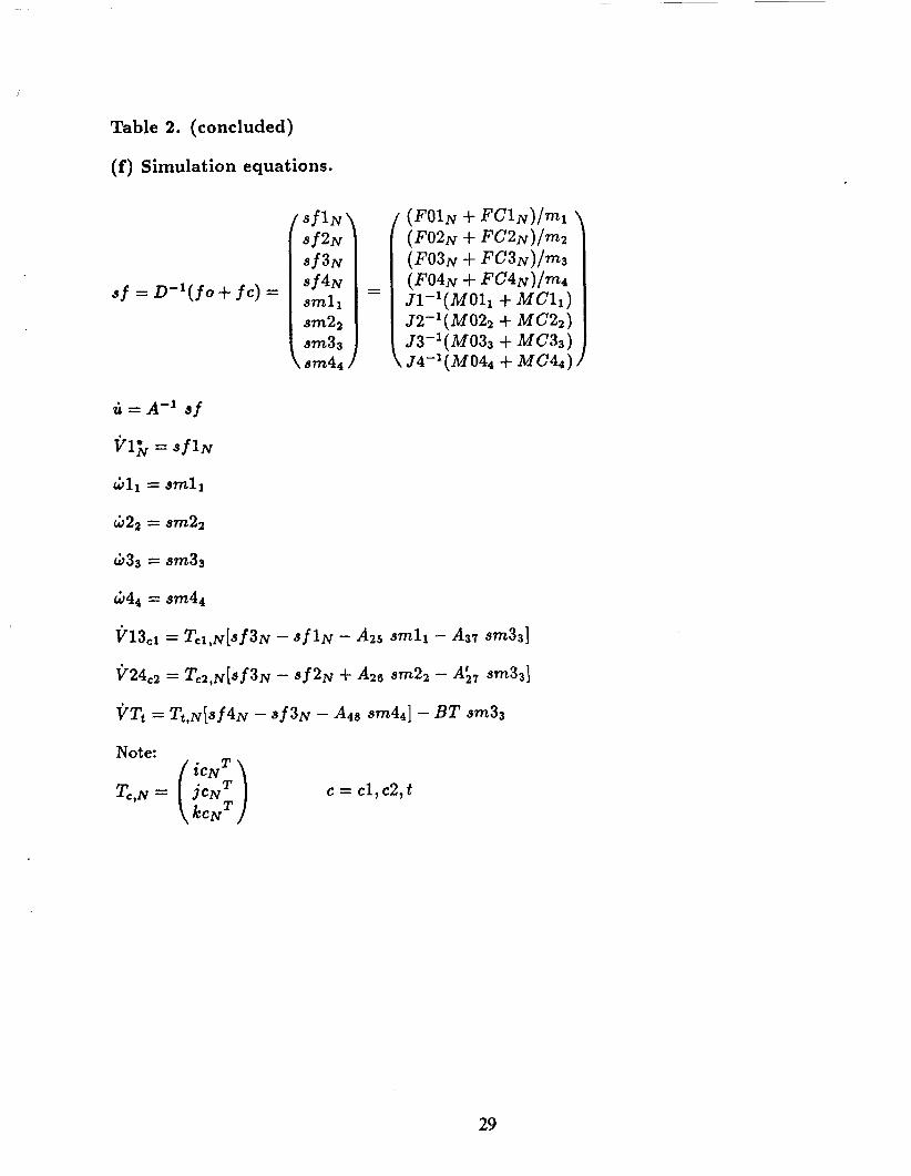
Table 2. (concluded)

(f) Simulation equations.

sf = D-'(fo + fc) =

Note:

Tc,N = (5) c = cl,c2,t

29

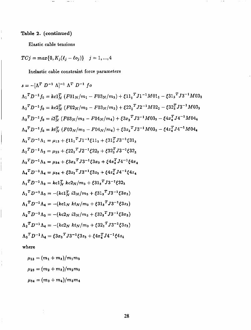
Secondly, the constraint force on the configuration, fc, is given in table 2e. In this example, qua- tion (11) or equations (18, 19) can be used for both elastic and inelastic cables, because c = m. Equa- tion (11) gives fc in terms of the four cable tensions and the coefficient matrix, H, given in table 3e. Here, H is also a basis of the constraint force space. A second basis is given formally by the rows of A-' corresponding to the cable stretch rates (rows 6, 9, 10, 12) and this is noted as A in the table 2e. The corresponding constraint force parameters can be identified (by equating the two expressions for fc) as the tether cable tensions, TC1 , TC2, and the Ft components of the constraint force, FT acting on the mangle at RS ; that is, the Ft components of the sum of bridle cable forces. Formulas for calculating cable line segments from u are included in the appendix, and these suffice to determine H and A , as well as {TCj, FT'}, for elastic cables. For inelastic cables, the constraint force parameters corresponding to A or H are given by equation (19). Expressions for the scalar elements of equation (19) corresponding to A are listed in the table. Similar expressions corresponding to H can be routinely generated, and the required inverse of the 4 x 4 matrix, [ A T D-' A], can be left to ordinary numerical methods without difficulty.

Finally, the simulation equations are assembled in table 2f. First the total specific force on the config- uration, sf, due to external forces, f o (which define the free body motion), and the interaction due to the suspensions, fc, are given. The vector elements of sf are denoted sfl , . . . , sm4. The simulation equations are given by expanding the relation u = A-' sf, representing equations (16) or (20). For inelastic cables, the cable stretching DOFs, i, (the components of V 13 along k c l , V 24 along kc2, and V T along i3 , kt ) are all theoretically zero.

Table 2 provides programmable simulation equations for a rigid body model of the dual lift system with spreader bar for elastic or inelastic cables. The expressions for fo, fc, ti can be rearranged further to reduce computational requirements. Repeated matrix-vector combinations are apparent in these expres- sions and are readily eliminated. Cross products occur frequently in the vector elements of Au, A , and an efficient generic routine for this is useful. Programming in terms of the mamx and vector objects of rigid body mechanics used in table 2 is possible with the language ADA ([35]), together with the matrix algebra package of [36].

The other dual lift systems, 5 and 7, of figure 1 are both three-body subsystems of system 6 obtained by deleting the load and bridle cables. System 5 can be represented by the same generalized velocity coordinates and equations as system 6 after deleting the six load-triangle coordinates and corresponding load forces and moments. System 7 is a specialization of system 5 with both cables attached at the same point on the load. Thus, all three dual lift systems are readily integrated in a singIe simulation.

5. CONCLUSIONS General simulation equations for slung load systems, derived from D' Alembert's principle, account for any suspension geometry including controllable geometry, cable elasticity, and choice of generalized co- ordinates. These equations generalize previous results for single helicopter systems and provide a new formulation for the case of inelastic suspensions, which is computationally more efficient than the conven- tional formulation, unifies the elastic and inelastic cable formulations, and is readily applied to the more complex dual lift and multilift systems.

Application of the general equations to the derivation of simulation equations for specific systems is demonstrated in the case of dual lift systems, and this previously difficult problem is seen to be tractable with these methods.

30

APPENDIX: SKEW-SYMMETRIC MATRICES AND

COORDINATE TRANSFORMATIONS The working equations of this report are given entirely in terms of vector functions from three-dimensional rigid body dynamics. These are expressed in a programmable form with the aid of skew-symmetric ma- trices and coordinate transformations. The general skew-symmetric matrix s'( z, y, z ) is defined from the scalar triplet ( 5, y, z ) as given in table Al . This allows scalar representation of the vector cross products ( V1 x V2 ) as shown in the table. The algebra of skew-symmetric matrices is consistent with correspond- ing relations from vector algebra, such as sums and reversals of cross products and triple product relations. Cross products pervade the dynamics in Coriolis velocities and accelerations and centrifugal accelerations. Corresponding scalar expressions are noted in the table. Cross products representing moments due to ca- bles occur in the equations of motion. A standardized formulation of this moment used in the present paper is given in the table. If cable C j applies tension TCj in the direction kcj at point Rj on body Bi, then its moment about the c.g. of Bi is given by

Mij = Ri'j x kcj TCj = [ij TCj

where the symbol cij is reserved for the moment action of cable C j on body Bi per unit tension. Euler angle transformations appear in all dynamic terms, and define the transformation of vectors given

by their coordinates in inertial space, to their coordinates in body or cable axes in terms of a sequence of single axis rotations. The primitive transformations for rotations about a single axis i , j , k of a right-handed orthogonal reference frame are denoted E1 ( a), E2 ( a), E3 ( a), and are given in table A2. Transformations to body axes Tb,N are given by the usual yaw, pitch, and roll rotation sequence of aeronautical usage, and are listed in table A2. For this report, cable axes are defined from inertial pitch and roll angles which locate the cable direction. This is a truncated Euler sequence and the corresponding transformation is given by nulling the yaw angle in Tb,N. In a simulation, Euler angles can be obtained from the kinematic angular rate relation tub( w bb) given in the table. Transformation rates occur througliout the inertia reaction term, Au, which represents Coriolis and centrifugal accelerations. The coordinates of an arbitrary vector, V , in frames &, FN are related by

The derivative

is the scalar counterpart of the usual vector Coriolis equation relating time derivatives relative to two dif- ferent coordinate frames. The second term can be identified as the effect of coordinate frame rotation, so that

To,* vb = (wb X v)b = To,b S ( W b b ) %

and this is valid for arbitrary vb.

VN = TN,b vb

VN = TN,b % i- TN,b vb

31

Table Al. Skew-symmetric matrices and cross products

0 --z

(-; : ") S ( Z , Y , 4 =

(V1 x V2), = S(Vl0)V2, = -(V2 x Vl), = -S(V2,)Vl,

Coriolis and centrifugal terms

( w x R ), = S( w,) Ro = -S( Ro) w,

( w x V), = S(w,)V, = -S(Vo)wo ( w x w ~ R ) , = S ~ ( w , ) R , = - S ( w , ) S ( R , ) w , = w ~ R w , - w 2 R,

Moment of cable Cj on body Bi about Ri *

Ti = body axes forBi Miji = (Ri *j x TCjkcj)i = S( Ri*j,) kcj,TCj = [ijiTCj

kCJ TCj * ----

32

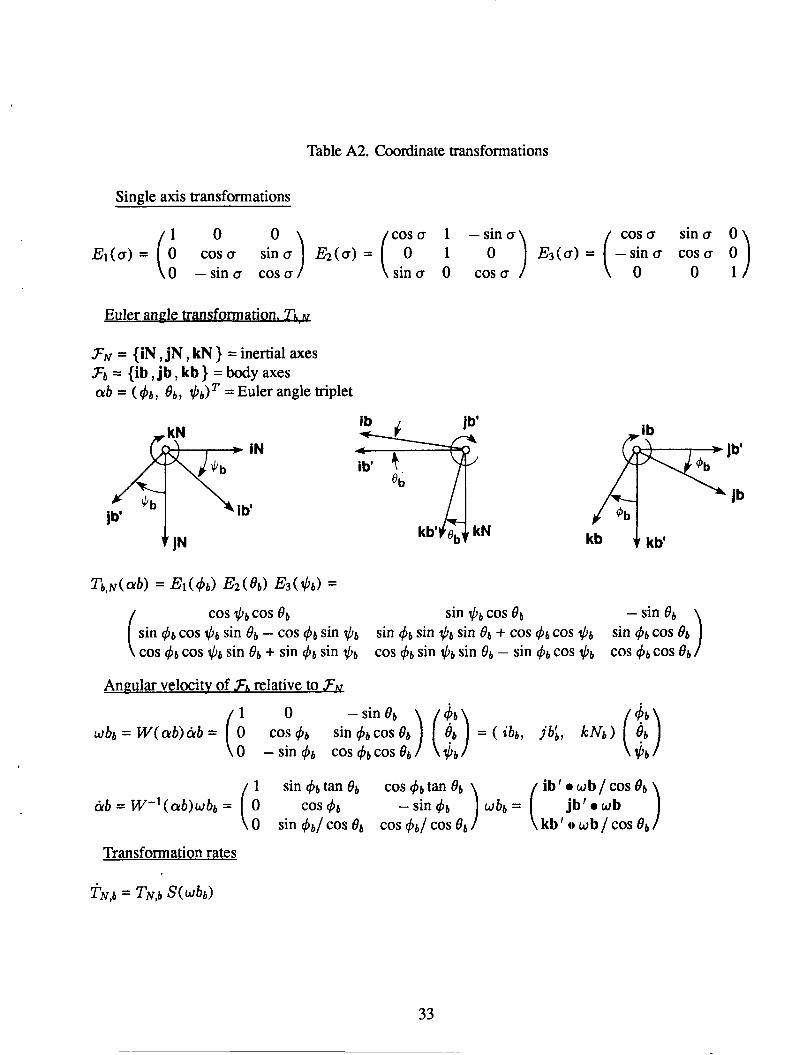
Table A2. Coordinate transformations

Single axis transformations

0 0 COSCY 1 -Yo) ( cos CY sin CY

cos0 sin.) a(0) = ( 0 1 &(CY) = - s i n 0 COSCY 0 sin CY 0 cos CY 0 0 1 0 -sin CY COSCY

Euler angle trm sformation. Th,u

FN = {iN, j N , kN 1 =inertial axes F6 = { ib , jb ,kb) =bodyaxes cub = ( 46, 66, $ 6 ) = Euler angle triplet

REFERENCES [ 1 ] Etkin, B.: Dynamics of Atmospheric Flight. Wiley and Sons, New York, 1972. [2] Sherman, P. F. et al.: Feasibility Study for Multiple Helicopter Heavy Lift Systems. Report R-136,

VERTOL Aircraft Corp. Philadelphia, PA, Oct. 1957.

[3] Maciolek, J. R. et al.: Preliminary Multilift Feasibility Study. Report SER 64460, Sikorsky Aircraft Company, Stratford, CT, Dec. 1969. (Proprietary).

[4] Meek, T.; and Chesley, G. B.: Twin Helicopter Lift System Study and Feasibility Demonstration. Report SER 64323, Sikorsky Aircraft Company, Stratford, CT, Dec. 1970 for U.S. Army Aviation Materiel Directorate, Fort Eustis, VA.

[SI Carter, E. S.: Implications of Heavy Lift Helicopter Size Effect Trends and Multilift Options for Filling the Need. Proceedings 8 t h European Rotorcraft Forum, Aix-en-Provence, France, Sept. 1982.

[6] Cicolani, L. S.; and Kanning G.: General Equilibrium Characteristics of a Dual Lift Helicopter Sys- tem. NASA TP-2615, July 1986.

[7] Curtiss, H. C.; and Warburton, E W.: Stability and Control of the Twin-Lift Helicopter System. Jour- nal of the American Helicopter Society, April 1985.

[8] Curtiss, H. C.: Studies of the Dynamics of the Twin-Lift System; 1983-1987. MAE TR-1840, De- partment of Mechanics and Aerospace Engineering, Princeton University, NJ, Oct. 1988.

[9] Meyer, G.; Hunt, R.; and Su, R.: Design of a Helicopter Autopilot by Means of Linearizing Transfor- mations. AGARD Conference Proceeding No. 23 1. “Advances in Guidance and Control Systems,” Oct. 1982.

[lo] Abzug, M. J.: Dynamics and Control of Helicopters With Two-Cable Sling Loads. AIAA Paper 70-929, July 1970.

[ 111 Nagabhushan, B. L.: Systematic Investigation of Models of Helicopter with a Slung Load. Ph.D. Thesis, Virginia Polytechnic inst. Blacksburg, VA, 1977.

[ 121 Prabhakar, A.: A Study of the Effects of an Underslung Load on the Dynamic Stability of a Helicopter. Ph.D. Thesis, Royal Military College of Science, Shrivenham, England, 1976.

[ 131 Weber, J. M.; Liu, T. Y.; and Chung, W.: A Math Simulation Model of a CH-47B Helicopter, vols. 1 and 2. NASA ‘I’M-84351, Ames Research Center, Moffett Field, CA, Aug. 1984.

[ 14) Briczinski, S. J.; and Karas, G. R.: Criteria for Externally Suspended Helicopter Loads. USAAMRDL TR-71-61, U.S. Army Mobility Research and Development Lab., Fort Eustis, VA, Nov. 1971.

[ 151 Shaughnessy, J. D.; Deaux, T. N.; and Yenni, K. R.: Development and Validation of a Piloted Simu- lation of an Helicopter and External Sling Load. NASA TP-1285, Jan. 1979.

College Park, Maryland, Spring 1980.

CA, Aug. 1985.

I [ 161 Sampath, P.: Dynamics of a Helicopter-Slung Load System. Ph.D. Thesis, University of Maryland,

[ 171 Ronen, T.: Dynamics of a Helicopter with a Sling Load. Ph.D. Thesis, Stanford University, Stanford, I

34

El81 Lewis, J.; and Martin, C.: Models and Analysis for Twin Lift Helicopter Systems. American Control Conference, San Francisco, CA, June 22-24, 1983. Proceedings of the Institue of Electrical and Electronics Engineers, vol. 3, pp. 1324-1325, New York, 1983.

[ 191 Menon, P. K. A.; Schrage, D. P.; and Prasad, J. V. R.: Nonlinear Control of a Twin-Lift Helicopter Configuration. Proceedings, AIAA Guidance and Control Conference, Minneapolis, MN, Aug. 1988.

[20] Schiehlen, W. 0.; and Kreuzer, E. J.: Symbolic Computerized Derivation of Equations of Motion. Dynamics of Multibody Systems, K. Magnus, ed., Springer-Verlag, NY, 1978.

[21] Kreuzer, E. J.; and Schiehlen, W. 0.: Generation of Symbolic Equations of Motion for Complex Spacecraft Using Formalism NEWEUL. Advances in Astronautical Sciences, vol. 54, 1983.

[22] Schiehlen, W. 0.: Computer Generation of Equations of Motion. NATO Institute on Computer Aided Analysis and Optimization of Mechanical System Dynamics. Iowa City, 1983. E. J. Haug, ed., Springer-Verlag, NY, 1984.

[23] Jerkovsky, W.: The Structure of Multibody Dynamics Equations. Journal of Guidance and Control, May 1978.

[24] Wittenburg, J.: The Structure of Multibody Dynamics Equations. Teubner, Stuttgart, Germany, 1977. [25] Haug, E. J.; Elements and Methods of Computational Dynamics. NATO Institute on Computer Aided

Analysis and Optimization of Mechanical System Dynamics (Iowa City, 1983), E. J. Haug, ed., Springer-Verlag, NY, 1984.

[26] Schwertassek, R.; and Roberson, R. E.: A Perspective on Computer-Oriented Multibody Dynamical Formalisms and their Implementations. IUTAM/IFToMM Symposium on the Dynamics of Multi- body Systems (Udine, 1985). G. Bianchi, W. Schiehlen, ed., Springer-Verlag, NY, 1986.

[27] MACSYMA Reference Manual. Mathlab Group, Laboratory for Computer Science, MIT, Cam- bridge, MA, Version Ten, vols. 1 and 2, Jan. 1983.

[28] Hussain, M. A.; and Noble, B.: Application of Symbolic Computation to the Analysis of Mechanical Systems, Including Robot Arms. NATO Institute on Computer Aided Analysis and Optimization of Mechanical System Dynamics. (Iowa City, 1983). E. J. Haug, ed., Springer-Verlag, NY, 1984.

[29] Lancashire, T. et al.: Investigation of the Mechanics of Cargo Handling by Aerial Crane-Type Aircraft. USAAVLABS TR-66-63, U.S. Army Aviation Material Lab., Fort Eustis, VA, Aug. 1966.

E301 Garnett, T. S.; Smith, J. M.; and Lane R.: Design and Flight Test of the Active Arm External Load Stabilization System. Proceeding 32 nd Annual AHS Forum, May 1976.

[31] Asseo, S. J.; and Whitbeck, R. F.: Control Requirements for Sling-Loa(d Stabilization in Heavy Lift Helicopters. AHS Journal, July 1973.

[32] Gabel, R.; and Wilson, G. J.: Test Approaches to External Sling Load Instabilities. AHS Journal, Oct. 1975.

[33] Kane, T. R.: Dynamics. 3rd Edition Stanford University, CA, Jan. 1978. [34] Bierman, G. J.: Factorization Methods for Discrete Sequential Estimation. Academic Press, New York,

1977.

35

[35] Cohen, N. H.: ADA as a Second Language. McGraw-Hill, New York, 1986. [36] Klumpp, A. R.: An Ada Linear Algebra Package Modeled After HAWS. JPL Report D-3729, Nov.

1986.

36

NASA N a 6 d Aamu6cs and Report Documentation Page Sppw ArhWsbaarn

1. Report No. NASA TM-102246

2. Government Accession No.

7. Author(s)

Luigi S . Cicolani and Gerd Kanning

19. Security Classif. (of this report)

Unclassified

9. Performing Organization Name and Address

20. Security Classif. (of this page)

Unclassified

Ames Research Center Moffett Field, CA 94035- lo00

12. Sponsoring Agency Name and Address

National Aeronautics and Space Administration Washington, DC 20546-0001

15. Supplementary Notes

3. Recipient’s Catalog No.

5. Report Date

February 1990 6. Performing Organization Code

8. Performing Organization Report No.

A-89270

10. Work Unit No.

505-66-01

1 1. Contract or Grant No.

13. Type of Report and Period Covered

Technical Memorandum

14. Sponsoring Agency Code

Point of Contact: Luigi S . Cicolani, Ames Research Center, MS 210-3 Moffett Field, CA 94035- lo00 (415) 604-5446 or FTS 464-5446

16. Abstract

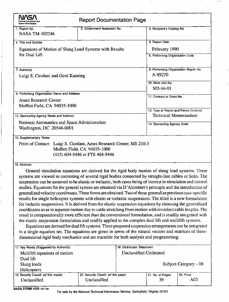
General simulation equations are derived for the rigid body motion of slung load systems. These systems are viewed as consisting of several rigid bodies connected by straight-line cables or links. The suspension can be assumed to be elastic or inelastic, both cases being of interest in simulation and control studies. Equations for the general system are obtained via D’Alembert’s principle and the introduction of generalized velocity coordinates. Three forms are obtained. Two of these generalize previous case-specific results for single helicopter systems with elastic or inelastic suspensions. The third is a new formulation for inelastic suspensions. It is derived from the elastic suspension equations by choosing the generalized coordinates so as to separate motion due to cable stretching from motion with invariant cable lengths. The result is computationally more efficient than the conventional formulation, and is readily integrated with the elastic suspension formulation and readily applied to the complex dual lift and multilift systems.

Equations are derived for dual lift systems. Three proposed suspension arrangements can be integrated in a single equation set. The equations are given in terms of the natural vectors and matrices of three- dimensional rigid body mechanics and are tractable for both analysis and programming.

17. Key Words (Suggested by Author(s)) I 18. Distribution Statement

Multilift equations of motion Dual lift Slung loads

Unclassified-Unlimited

Subject Category - 08

21. No. of Pages 22. Price

39 1 A03 I I I

IASA FORM 1626 OCT86 For sale by the National Technical Information Service, Springfield, Virginia 22161