Equilibrium Counterfactuals:

Joint Estimation and Control in Structural Models∗

Gilles Chemla

Imperial College, DRM/CNRS, and CEPR.

Christopher A.Hennessy

LBS, CEPR, and ECGI

October 2018

Abstract

The objective of applied structural microeconometrics is to identify policy-invariant parame-

ters so alternative policies can be assessed. As we show, the practice of treating policy changes

as zero probability "counterfactuals" violates rational expectations: Agents inside the model

understand policy changes are positive probability events which the structural estimation is

intended to inform. We analytically characterize the implications for moment-based parameter

inference. As shown, if a policy change is optimal, inference is biased. Further, the standard

identifying assumption, constant partial derivative sign, is neither necessary nor suffi cient with

policy control. We offer an alternative identifying assumption: constant total differential sign

with inference-policy feedback. It is shown that under this assumption, rational expectations can

be imposed computationally (algorithmically) to generate unbiased inference and optimal policy.

The quantitative importance of these effects in applied settings is illustrated by calibrating the

Leland (1994) model to the Tax Cuts and Jobs Act of 2017.

∗We thank seminar participants at the CEPR ESSET Meetings, Imperial, Oxford, and Dauphine.

1

1. Introduction

In recent years, there have been intense debates regarding alternative microconometric method-

ologies, particularly between advocates of reduced-form quasi-experimental methods and those

advocating structural models. The natural experiment camp contends that the Achilles heel of

structural work is an inability to deal with key issues concerning selection and heterogeneity. Con-

versely, the structural camp has argued that an important weakness of reduced form work is that

it faces severe limitations on external validity. For examples, see Keane (2010) and Rust (2010).

Of course, limits on external validity give rise to challenges associated with using reduced-

form methods to assess alternative “counterfactual” policies. In light of these challenges, the

reduced-form school often focuses on so-called causal questions (“Is a particular causal mechanism

operative?”) and avoids any formal treatment of normative questions. Or rather, reduced-form

evidence is often left as “suggestive”of directions for future policy.

In contrast to reduced-form econometricians, the structural econometrician first writes down

an explicit model that, ideally, mimics the real-world data generating process confronting agents,

including an accounting for technologies, tastes, constraints, information sets, and shocks. The

structural econometrician then selects empirical moments that are informative about unknown

parameters and minimizes the distance between model-implied moments and the selected empirical

moments. The notion of informativeness is formalized and analyzed by Gallant and Tauchen

(1996), for example. Kahn and Whited (2017) provide the following heuristic description of moment

selection: “From an intuitive perspective, this identification condition means that the relations

between the moments and parameters need to be steep and monotonic...”

Advocates often argue that a key relative advantage of structural inference over reduced-form

inference is that structural models allow for a rigorous assessment of alternative policy options

that a government may adopt in the future. After all, the objective of structural inference is

to estimate the magnitudes of policy-invariant (“deep”) parameters. With unbiased estimates of

policy-invariant parameters in-hand, alternative policies can be fed into the model and welfare

implications can be evaluated. This procedure is nicely summarized by Sargent (1984):

Once estimates of the free parameters of agent’s objectives and constraints have

been obtained, the aim is to use them to analyze how the economy would behave under

1

hypothetical strategies for setting government policy variables that are different from

the one evident in the sample period.

In this paper, we explore a logical contradiction that exists at the core of structural microecono-

metric methods when these methods are used in a manner consistent with their alleged advantage

over reduced-form methods, as tools for assessing policy alternatives and for giving policy advice.

To see the contradiction, consider that in specifying the decision problem of agents inside her

model, the structural econometrician must specify government policy. Critically, it is customary to

parameterize the structural model according to the status-quo government policy. But if the status

quo government policy will remain in place, the econometric analysis is moot and the alleged ad-

vantage of structural methods in guiding policy is of no real value. Conversely, if “counterfactual”

policy changes are positive probability events, agents with rational expectations will understand

this, resulting in a change in their optimal actions.

This argument is in the spirit of Sargent (1987) who states, “There is a logical diffi culty in using

a rational expectations model to give advice, stemming from the self-referential aspect of the model

that threatens to absorb the economic adviser into the model... That simultaneity is the source

of the logical diffi culties in using rational expectations models to give advice about government

policy.”Striking a pessimistic note, Sargent (1984) stated, “I am unaware of an alternative approach

to Sims or to rational expectations econometrics that avoids these contradictions and tensions.”

These philosophical and logical diffi culties apparently led Sargent to shy away from the use of

macroeconometric models for the purpose of informing monetary and fiscal policy decisions. For

example, Sargent (1994) states, “That’s a hard problem. I don’t make policy recommendations.”1

The pessimistic conclusion reached by Sargent (1994) was apparently not shared by all in the

profession at the time. For example, Cooley, LeRoy and Raymon (1984) argued that, “Contrary to

Lucas, there is no reason in principle why economists should decline to analyze specific historical

episodes—that is, should be unwilling to rank different policy sequences evolving out of a common

past (of course, this is not to minimize the practical diffi culties attending such an exercise).”

Apparently, this set of philosophical debates has largely escaped the attention of structural

microeconometricians. This state of affairs is not entirely surprising given that the debates between

1Quoted in Sent (1998).

2

Sargent and Sims, amongst others, centered on the correct interpretation and utilization of vector

autoregressions in the setting of monetary and fiscal policy.

With the preceding discussion in mind, the objectives of this paper are multi-fold. First,

we develop a tractable general framework for incorporating agents’ rational expectations into a

structural microeconometric model that will be used for the purpose of policy advice. Second, and

more importantly, we move well beyond highlighting philosophical contradictions by characterizing

analytically the precise nature of bias that will arise if the structural econometrician engages in

the customary practice of treating agents as being unaware of the potential for an endogenous

policy change. Third, we discuss how, within the context of moment-based microeconometrics,

the philosophical challenges can be circumvented, while achieving unbiased parameter inference

and optimal policy. Finally, we show that the standard moment monotonicity condition is neither

necessary nor suffi cient for parameter identification in the context of joint estimation and policy

control, and we offer an alternative moment selection criterion.

In the model, there is a continuum of atomistic firms that will be observed by an econometrician.

The firms are privately endowed with a single deep structural parameter, with knowledge of this

parameter being suffi cient for the government to set policy optimally. The econometrician will

observe an empirical moment which will serve as the basis for her parameter inference. Importantly,

under technical assumptions, the empirical moment is suffi cient for the government to achieve

unbiased parameter inference and the first-best policy.

When the model opens, the policy variable is initially equal to the pre-determined status quo

value. Next, nature draws the unknown parameter u from the real line. The firms then privately

observe this parameter and choose their preferred actions non-cooperatively. The econometrician

then observes a moment m arising from the endogenous decisions of the firms. Importantly, the

moment is assumed to satisfy the standard monotonicity condition (constant sign of ∂m/∂u). The

econometrician then matches her model moment with the observed empirical moment in order

to draw an inference u of the unknown parameter u. Finally, with some positive probability the

government will subsequently enjoy an opportunity to re-set its policy variable based upon the

econometric inference.

We begin the analysis by characterizing the bias that arises if the structural microeconometrician

treats policy changes as counterfactual events and thus fails to impose the assumption that agents

3

have rational expectations regarding future policy. Indeed, within the model, firms know the

true value of the parameter u. Based upon this information, firms can correctly anticipate the

econometrician’s inference u(u). More generally, firms can rationally anticipate the function u(·)

which determines the econometrician’s inference for each possible realized value u. Armed with

this knowledge, the firms then correctly anticipate what policy the government will implement if it

enjoys policy discretion.

As shown, the failure to impose rational expectations results in u(u) 6= u at all points except the

one possible realization of the unknown parameter, we call it u0, that would justify the government

maintaining the status quo. Intuitively, in this exceptional (measure zero) case, the econometrician

will not violate rational expectations since parameterizing the model as if the status quo will remain

in place in the future is actually correct here. At all other points u ∈ R, inference is biased.

We next address head-on the “practical diffi culties”alluded to by Cooley, LeRoy and Raymon

(1984), doing so in the context of applied structural microeconometrics. This allows us to offer

a simple catalog of the nature of bias as a function of the properties of the moment function m

and the government policy function g. The central insight is as follows. In a rational expectations

equilibrium, the empirical moment first varies directly with changes in the parameter u. This direct

effect, mu, is accounted for by the structural econometrician. However, the empirical moment also

varies indirectly through feedback from the inference (u) to discretionary government policy (g(u))

to the empirical moment. Thus we write the empirical moment as m[u, g(u(u))]. It is this indirect

effect arising from policy control, mgg′u′, that is generally ignored.

The nature of bias depends on the nature of the indirect effect. There are three cases to consider.

In the first case, the sign of the indirect effect is opposite to that of the direct effect. Here, the

estimated parameter overshoots for u < u0 and then undershoots for u > u0 (and recall, u0 justifies

the status quo). Intuitively, the modeler incorrectly treats small changes in the empirical moment

to small changes in u because she here fails to account for the countervailing indirect effect. In the

second case, the indirect effect is small in absolute value and has the same sign as the direct effect.

Here, the estimated parameter undershoots for u < u0 and overshoots for u > u0. Intuitively, the

modeler incorrectly treats large changes in the empirical moment to large changes in u because she

here fails to account for the amplifying indirect effect. In the third case, the indirect effect is large

in absolute value and has the same sign as the direct effect. Here, the estimated parameter actually

4

decreases with the true parameter, and it is actually possible for an equilibrium to arise where the

estimated parameter always has the wrong sign. The subtle intuition for this case is provided in

the body of the paper.

We illustrate the quantitative significance of these effects by considering an econometrician

whose objective is to infer bankruptcy costs using the canonical structural model of Leland (1994).

In particular, we consider the recent cut in the corporate income tax rate implemented under the Tax

Cuts and Jobs Act of 2017. Here the structural microeconometrician backs out implied bankruptcy

costs from observed values of corporate interest coverage ratios. By assumption, the econometrician

knows the underlying real technology but fails to impose the assumption of rational expectations on

the part of firms. In our calibrated example, this leads to an eight-fold overstatement of bankruptcy

costs. Intuitively, firms rationally anticipate a tax cut and thus choose low leverage in light of the

low value of future debt tax shields. Neglecting this fact, the econometrician mistakenly infers that

the low leverage stems from extremely high bankruptcy costs.

Importantly, we show that, at least in terms of structural microeconometrics, the paradoxes

discussed by Sargent (1984, 1987) are not insurmountable. In particular, we describe how unbiased

parameter inference and optimal government policy can be achieved. Essentially, the econome-

trician must insist that the beliefs of the agents inside her model are consistent with the policy

advice she will give. This involves recognizing that the observed moment will vary directly with the

unknown parameter u and also with agents’rational expectation of government policy changes in

light of (correct) inference of the structural parameter. Related to this point, the standard moment

monotonicity condition, which focuses on partial derivatives of moments, is neither necessary nor

suffi cient for parameter identification, and we propose total derivatives, cum policy feedback, as

the correct moment selection criterion in the context of joint estimation and control exercises.

It is worth emphasizing at the outset that our focus below on structural parameter inference

for the purpose of government policy setting towards firms is simply to fix ideas. In broad details,

the model applies to any entity attempting to infer some parameter for a group of agents, provided

that the agents are forward-looking rational maximizers, and provided that the entity will act based

upon its parameter inference with positive probability. For example, firms might be interested in

estimating policy-invariant consumer parameters with the goal of evaluating alternative pricing

5

strategies, product characteristics, or marketing expenditures.2 Alternatively, governments might

be interested in estimating deep parameters determining labor supply, human capital investments,

or the number of offspring.3

It is also worth emphasizing at the outset that our model is intended to be forward-looking in

terms of its application. That is, it might be plausibly argued that in many settings the link between

econometric evidence and decision-making is weak at the present time. However, most economists

strongly advocate a move toward systematic evidence-based decision-making by governments and

firms. Moreover, it is clear that governments notwithstanding, modern firms are increasingly moving

toward data-driven decision-making, or fail to do so at their own peril. Our framework can be seen

as capturing the types of problems of econometric inference that will intensify as systematic data-

driven decision-making becomes commonplace, and as the measured agents understand this to be

taking place. The specific focus of this paper is on potential bias in structural parameter inference.4

The rest of the paper is as follows. Section 2 describes the economic setting. Section 3 char-

acterizes the nature of bias if the econometrician fails to impose rational expectations. Section

4 shows how, under technical conditions, unbiased parameter inference and first-best government

policy can be achieved through a fully-consistent application of rational expectations. In addi-

tion, Section 4 shows how traditional moment selection criteria are altered when one moves away

from a pure estimation setting to a setting with joint estimation and control. Section 5 presents a

quantitative example.

2. The Economic Setting

We consider a univariate parameter inference problem where the econometric model is exactly

identified. The first subsection describes timing and technology assumptions. The second subsection

illustrates how the general framework maps to a specific applied microeconometric problem.

2.1. Timing, Technology, and Beliefs

There is a representative sample consisting of a continuum of atomistic firms privately endowed

with a policy-invariant (“deep”) structural parameter. Knowledge of this parameter is suffi cient

for the government to set policy optimally.

2See Chintagunta, Erdem, Rossi and Wedel (2006) for a survey of structural methods in marketing.3See Wolpin (2013).4Chemla and Hennessy (2018) analyze natural experiments.

6

An econometrician will observe an empirical moment derived from the measured actions of the

sample firms. To fix ideas, one can think of the moment as being the sample mean of investment,

new employees, R&D, or leverage. In practice, moments such as variance, skewness, or kurtosis

may also be informative about deep parameters. In the context of indirect inference, the moment

can be the coeffi cient obtained when firm decision variables are regressed on observable covariates,

such as the coeffi cient on market-to-book (Q) in an investment regression. Below, specific examples

are provided.

The econometrician has developed a structural model and will match her model-implied mo-

ment with the observed empirical moment. Importantly, under conditions derived below, if the

econometrician were to impose rational expectations in a fully internally consistent manner, this

moment matching procedure would allow her to infer the true value of the deep parameter and the

government would then be able to correctly determine the optimal policy.

The atomistic firms are rational, forward-looking, and act non-cooperatively. Each atomistic

firm correctly understands it cannot change the moment observed by the econometrician by uni-

laterally changing its own action.

The deep parameter, denoted u, is common to all sample firms. However, this assumption does

not preclude firm heterogeneity. For example, firms may be identical ex ante but face idiosyncratic

shocks ex post. Alternatively, firms may face idiosyncratic shocks that alter their measured actions.

Finally, firm-level parameters might be, say, multiples of a common “aggregate”parameter u, e.g.

ui = εiu where εi is a firm-specific scalar known by firm i. An alternative technological assumption,

not adopted here, is that each firm receives a noisy signal of the common parameter u. In such

a setting, as in the present setting, parameter inference would need to account for feedback from

inference to the policy variable.

The parameter u represents the realization of a random variable u with cumulative distribution

function Ψ with a strictly positive density ψ on R with no atoms. The realized parameter u is

privately observed by each of the sample firms, but unobservable to the econometrician and the

government. Below, u(u) denotes an equilibrium parameter inference by the econometrician in the

event that u = u, with u(·) denoting an equilibrium inference function.

Timing is as follows. When the model opens at time t = 0, the government policy variable

is initially equal to the pre-determined status-quo γ0 ∈ Γ where the set of feasible government

7

policies Γ ≡ (γ, γ). Next, nature draws u according to the distribution function Ψ. Each sample

firm i then chooses an optimal pre-inference action φi. This action can be multi-dimensional. The

econometrician then observes the empirical moment m, which is derived from the pre-inference

actions of the sample firms. Next, the econometrician will attempt to match her model-implied

moment with the empirical moment, resulting in parameter inference u. The econometrician then

reports u to the government. All of these events take place at the initial time t = 0.

Time is either discrete or continuous and the horizon can be finite or infinite. There is an

independent stochastic process d such that for all t ≥ 0, dt ∈ {0, 1}. Let

t∗ ≡ inft≥0

dt = 1.

At time t∗, the government enjoys a one-time opportunity to permanently re-set the policy variable,

having already received the econometrician’s report. At all prior dates, policy is fixed at the status

quo γ0.

The government’s equilibrium choice of discretionary policy is denoted γ∗. Under the stated

assumptions, government policy post-inference is an independent stochastic process γt with

t < t∗ ⇒ γt = γ0 (1)

t ≥ t∗ ⇒ γt = γ∗.

No sample firm receives any signal that is informative about γ∗ aside from u. Thus, firm policy

expectations are homogeneous. With this in mind, let γ denote the value of γ∗ anticipated by the

sample firms conditional upon their knowledge of u.

The optimal pre-inference action of firm i can be expressed as

φi(u, γ; γ0) (2)

where the subscript i captures idiosyncratic shocks and the semi-colon separates variables from the

constant γ0.

It is assumed that observation of a continuum of sample firms is suffi cient to ensure that

any idiosyncratic shocks have no effect on the observed moment, so that m can be expressed as

m(u, γ; γ0). For brevity, the constant γ0 will be suppressed and the empirical moment will be

8

represented by the following mapping:

m : R× Γ→ R. (3)

The first argument in the moment function m is the unknown parameter u ∈ R. The second

argument in the moment function is anticipated discretionary government policy γ ∈ Γ.

The following assumption ensures the setting considered is seemingly-ideal.

Assumption 1. The model-implied moment function is identical to the empirical moment function

m : R × Γ → R. Moreover, for each γ ∈ Γ, the function m(·, γ) is continuously differentiable and

strictly monotonic.

The first part of Assumption 1 states that the structural model is correct. In particular, from

Assumption 1 it follows that if the model were to be parameterized with a correct stipulation

of u and γ, the model-implied moment would match the empirical moment. The second part of

Assumption 1 is the traditional structural identifying assumption that m(·, γ) is strictly monotonic.

We next characterize how the moment varies with anticipated discretionary government policy.

Assumption 2. For each u ∈ R, m(u, ·) is a continuously differentiable strictly monotonic func-

tion.

Notice, the setting considered is quite general. For example, as in Blume, Easley and O’Hara

(1982), one can think of the sample firms as solving canonical finite or infinite horizon dynamic

programming problems with differentiable policy functions where monotone comparative statics

apply and carry over to m. Nevertheless, it is worth emphasizing that in order for Assumption 2

to hold, it must be the case that the sample firms are solving forward-looking problems in which

anticipated discretionary government policy γ enters as a relevant parameter in their program,

either through periodic payoff functions, constraint functions, and/or transition functions.

The function g : R→ Γ represents optimal discretionary government policy. If the government

had the ability to directly observe u, its optimal discretionary policy would be g(u). Of course, the

sample firms will have already chosen their pre-inference actions φi. However, the government cor-

rectly understands that should it enjoy discretion, its policy choice γ∗, in addition to the parameter

u, will determine the post-inference actions of the sample firms and/or other agents in the econ-

omy, e.g. future generations of firms. The function g represents the socially optimal u-contingent

government policy in light of the relevant tradeoffs. The following assumption is imposed.

9

Assumption 3. The optimal government policy g is a continuously differentiable strictly monotonic

function mapping R onto Γ.

The government is presumed to believe that the standard moment matching exercise will allow

the econometrician to deliver a correct estimate of the unknown parameter. Critically, Assumption

1 would seem to imply that this confidence is justified. After all, the model moment function is

equal to the empirical moment function, and the moment is monotone in the unknown parameter.5

We have the following assumption.

Assumption 4. The government chooses discretionary policy optimally given its belief that for all

u ∈ R, u(u) = u.

From Assumption 4 it follows that for all u ∈ R, the endogenous discretionary policy of the

government is

γ∗(u) = g[u(u)]. (4)

An alternative interpretation of condition (4) is that the function g represents equilibrium policy

outcomes from an extensive form game in which the econometrician’s parameter estimate is fed into

the political decision-making process. This alternative interpretation would not alter the charac-

terization of bias below, but would necessarily rule out characterization of the welfare consequences

of biased parameter inference.

We posit that real-world firms form rational expectations. In particular, real-world firms know

that the government may enjoy policy discretion at some future date. They also know the govern-

ment will place full faith in the econometrician’s structural parameter estimate u, and will then

input this estimate into the policy function g. The following assumption formalizes this specification

of firm beliefs.

Assumption 5 [Firm Rational Expectations]. For all u ∈ R, real-world firms correctly

anticipate discretionary government policy, with

γ(u) = γ∗(u) = g[u(u)]. (5)

5See Gallant and Tauchen (1996) and Kahn and Whited (2017) for moment monotonicity as an identifying as-

sumption.

10

The first equality in the preceding equation ensures that γ(·) satisfies rational expectations. The

second equality reflects how discretionary government policy γ∗ will actually be formed in equilib-

rium, with u(u) being fed into g. Effectively, under rational expectations, the real-world firms infer

the econometrician’s parameter estimate which allows them to correctly anticipate discretionary

government policy.

From the preceding equation it follows that the empirical moment observed by the econometri-

cian is:

m[u, γ(u)] = m[u, γ∗(u)] = m[u, g(u(u))]. (6)

In reality, the post-inference government policy follows the stochastic process described in equa-

tion (1). The real-world sample firms have rational expectations and understand this. However,

we assume the econometrician departs from rational expectations by parameterizing her structural

model according to the status-quo. Below we formally state this important assumption.

Assumption 6 [Status Quo Parameterization]. Firms inside the structural model anticipate

that the status quo will be maintained even if the government enjoys policy discretion, believing

γ = γ0.

Notice, by parameterizing her model according to the status quo, the econometrician implicitly

treats the firms as being unaware of her own activities and the policy function they are intended to

serve, informing the government’s discretionary decisions. Below we analyze the implications for

parameter inference and government policy.

From the preceding discussion it follows that for all u ∈ R, the structural econometrician’s

parameter estimate will be derived from the following inference equation

m[u, γ∗(u)] = m[u(u), γ0] (7)

or

m[u, g(u(u))] = m[u(u), γ0]. (8)

The left side of the preceding equation is the observed empirical moment. The empirical moment

reflects the fact that the sample firms will choose their pre-inference actions optimally given the true

parameter value u and their correct anticipation of discretionary government policy (Assumption

5). The right side of the preceding equation is the model-implied moment under the status quo

11

parameterization (Assumption 6). The estimated parameter u(u) is chosen so that the model

implied moment is equal to the observed empirical moment.

2.2. Example: Inferring Labor Adjustment Costs

Consider an econometrician who wants to estimate a labor adjustment cost parameter u based

upon some empirical moment, say, the average gross increase in firm or plant-level employment.6

In particular, the econometrician would like to infer the marginal cost to firms of complying with

government employment regulations. For simplicity, assume that just after receiving the econome-

trician’s report, the government will enjoy policy discretion with probability p > 0.

This exercise is in the spirit of Hammermesh (1989), Blanchard and Portugal (2001), and

Ejarque and Portugal (2007) who estimate parameters of labor adjustment cost functions and then

use the estimates as the basis for making policy recommendations regarding labor market reforms.

Of course, although the focus of the example is on labor adjustment costs, similar arguments

would apply to moment-based inference of capital stock adjustment cost parameters. See Adda

and Cooper (2003) for an overview.

Let φi denote the number of workers hired by firm i. Prior to inference by the econometri-

cian, each sample firm i is assumed to solve the following program featuring a standard quadratic

technology:

maxφi

φiq −1

2[pγ + (1− p)γ0]N(u)(φ− εi)2. (9)

In the preceding equation, q > 0 represents the shadow value of a hired worker—the expected present

value of worker marginal product less wages. For simplicity, assume q is known to the econome-

trician.7 Marginal costs of complying with labor market regulations is captured by the product of

expected units of regulation and the function N measuring the marginal cost of complying with

each unit of regulation, again expressed in present value terms. The function N is, say, the normal

cumulative distribution function. Finally, εi captures a mean-zero firm-specific shock to labor costs.

In this way, the structural estimation allows for firm heterogeneity.

The sample firms will solve the preceding program, and the econometrician will observe the

6We focus here on hiring costs since firing costs may well differ.7Or the econometrician is willing to rely upon existing estimates of this parameter.

12

following empirical moment:∫i

φidi = m[u, γ∗(u)] = [pg(u(u)) + (1− p)γ0]−1[N(u)]−1q. (10)

Evaluated at parameterization u′, the model implied moment is:

m(u′, γ0) = [γ0]−1[N(u′)]−1q. (11)

The econometrician chooses her parameter estimate so that empirical moment is just equal to the

model-implied moment. It follows that in the present context the inference equation (8) is:

[pg(u(u)) + (1− p)γ0]−1[N(u)]−1q = [γ0]−1[N(u(u))]−1q. (12)

Rearranging terms in the preceding equation we find

u(u) = N−1[pg(u(u)) + (1− p)γ0

γ0×N(u)

]. (13)

From which it follows that

u(u) = u⇔ g(u) = γ0. (14)

That is, parameter inference is unbiased at point u if and only if the status quo is truly optimal at

that point. Of course, such u occurs with probability zero, a distressing finding.

The next subjection offers a more general and precise characterization of the bias.

3. Bias Characterization

This section characterizes the nature of parameter inference and associated policy outcomes if

the structural model fails to impose the assumption that firms have rational expectations.

Before proceeding, it will be convenient to express the differential form of the inference equation.

In particular, under technical conditions derived below, there will exist a continuously differentiable

function u(·) satisfying the inference equation (8). Assuming such a function exists, we have the

following differential form:

mu[u, g(u(u))] +mγ [u, g(u(u))]g′[u(u)]u′(u) = mu[u(u), γ0]u′(u). (15)

The differential form of the inference equation makes clear the potential for bias. The right side

captures the econometrician’s faulty inference procedure which is predicated upon the incorrect

13

assumption that firms expect the status quo to be maintained with probability 1. Thus, she

incorrectly imputes any change in the observed moment to the direct effect as captured by the

partial derivative, mu. The left side of the preceding equation captures the true total differential

of the empirical moment with respect to u. If u is perturbed, there will be direct effect on the

moment as captured by the first term, mu. In addition, the empirical moment will vary further

due to the rational anticipation of firms that government policy will change based upon changes in

the econometrician’s parameter inference. This inference-policy feedback effect is captured by the

second term on the left side of the equation (mγg′u′).

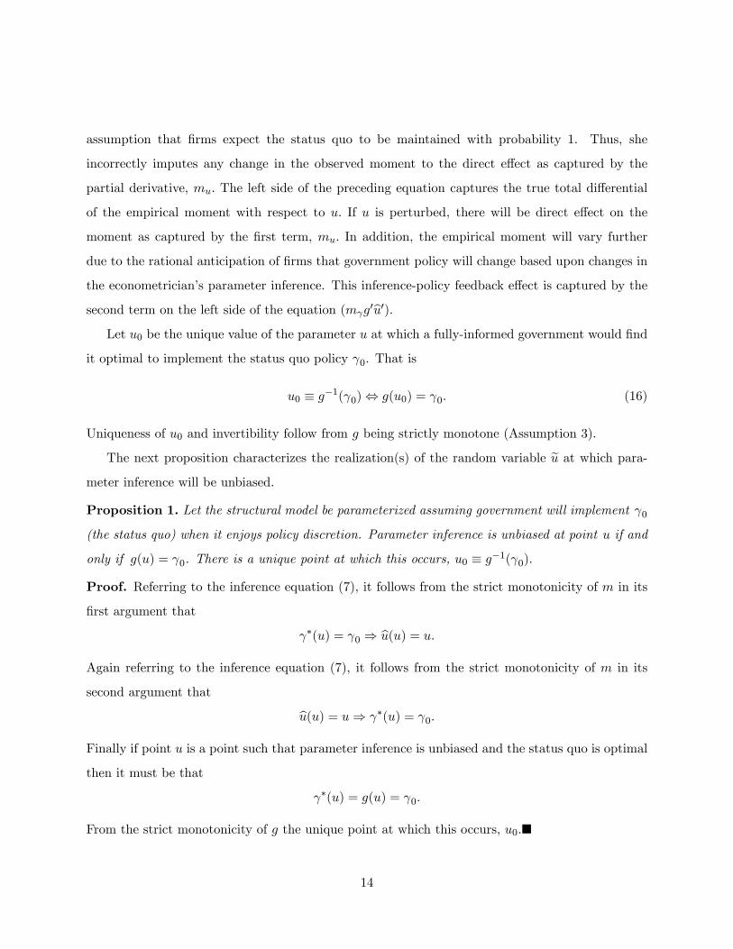
Let u0 be the unique value of the parameter u at which a fully-informed government would find

it optimal to implement the status quo policy γ0. That is

u0 ≡ g−1(γ0)⇔ g(u0) = γ0. (16)

Uniqueness of u0 and invertibility follow from g being strictly monotone (Assumption 3).

The next proposition characterizes the realization(s) of the random variable u at which para-

meter inference will be unbiased.

Proposition 1. Let the structural model be parameterized assuming government will implement γ0

(the status quo) when it enjoys policy discretion. Parameter inference is unbiased at point u if and

only if g(u) = γ0. There is a unique point at which this occurs, u0 ≡ g−1(γ0).

Proof. Referring to the inference equation (7), it follows from the strict monotonicity of m in its

first argument that

γ∗(u) = γ0 ⇒ u(u) = u.

Again referring to the inference equation (7), it follows from the strict monotonicity of m in its

second argument that

u(u) = u⇒ γ∗(u) = γ0.

Finally if point u is a point such that parameter inference is unbiased and the status quo is optimal

then it must be that

γ∗(u) = g(u) = γ0.

From the strict monotonicity of g the unique point at which this occurs, u0.�

14

The intuition for the preceding result is as follows. At any realization of u other than u0, real-

world firms anticipate the government will implement a policy different from the status quo should

it enjoy policy discretion. The real-world firms then change their optimal behavior accordingly,

leading to changes in the observed moment. However, under Assumption 6, the econometrician

fails to take the inference-policy feedback effect into account, leading to bias.

Having established parameter inference will only be unbiased at point u0, the next proposition

provides insight into the nature of bias at all other u ∈ R.

Proposition 2. Let the inference equation (7) be satisfied at point u by u(u). If mumγ > 0, then

γ∗(u) < γ0 ⇒ u(u) < u

γ∗(u) > γ0 ⇒ u(u) > u.

If mumγ < 0, then

γ∗(u) < γ0 ⇒ u(u) > u

γ∗(u) > γ0 ⇒ u(u) < u.

Proof. There are four cases to consider. Suppose first m is increasing in both arguments. Then

from the inference equation (7) it follows

γ∗(u) < γ0 ⇒ m[u, γ0] > m[u, γ∗(u)] ≡ m[u(u), γ0]⇒ u(u) < u

γ∗(u) > γ0 ⇒ m[u, γ0] < m[u, γ∗(u)] ≡ m[u(u), γ0]⇒ u(u) > u.

Suppose next m is decreasing in both arguments. Then

γ∗(u) < γ0 ⇒ m[u, γ0] < m[u, γ∗(u)] ≡ m[u(u), γ0]⇒ u(u) < u

γ∗(u) > γ0 ⇒ m[u, γ0] > m[u, γ∗(u)] ≡ m[u(u), γ0]⇒ u(u) > u.

Suppose next m is decreasing in its first argument and increasing in its second argument. Then

γ∗(u) < γ0 ⇒ m[u, γ0] > m[u, γ∗(u)] ≡ m[u(u), γ0]⇒ u(u) > u

γ∗(u) > γ0 ⇒ m[u, γ0] < m[u, γ∗(u)] ≡ m[u(u), γ0]⇒ u(u) < u.

15

Suppose finally m is increasing in its first argument and decreasing in its second argument. Then

γ∗(u) < γ0 ⇒ m[u, γ0] < m[u, γ∗(u)] ≡ m[u(u), γ0]⇒ u(u) > u

γ∗(u) > γ0 ⇒ m[u, γ0] > m[u, γ∗(u)] ≡ m[u(u), γ0]⇒ u(u) < u.�

The intuition behind the preceding result is as follows. Per Assumption 6, the econometrician’s

structural model incorrectly stipulates firm beliefs at any u at which the discretionary government

policy will differ from the status quo. This incorrect stipulation of beliefs leads to incorrect inference.

For example, taking the first part of the proposition, suppose the empirical moment function m is

increasing (decreasing) in both arguments. Then if, say, γ∗(u) > γ0, the moment will be higher

(lower) than would be inferred based upon the direct effect mu, causing u to overshoot u. Taking

the second part of the proposition, suppose that mu > 0 and mγ < 0. Then if, say, γ∗(u) > γ0,

the moment will be lower than would be inferred based upon the direct effect mu, causing u to

undershoot u.

The preceding proposition characterizes u at a particular point u where the inference equation

(7) has a solution. However, as shown below, the inference equation need not have a solution. With

this in mind, the following lemma offers a suffi cient condition such that there exists a (continuously

differentiable) function u(·) that satisfies the inference equation pointwise for all u ∈ R.

Lemma 1. Let mumγ < 0 and g′ > 0 or let mumγ > 0 and g′ < 0. Then there exists a continuously

differentiable strictly monotonic increasing function u(·) satisfying the inference equation (7) for

all u ∈ R. The function u(·) has slope in (0, 1) at u0.

Proof. Consider the following function which is continuously differentiable in its two arguments

F (u, z) ≡ m[u, g(z)]−m(z, γ0).

Any root z of the preceding equation represents a solution to the inference equation (7). We

know (Proposition 1) the root at u0 is u0. Consider next arbitrary u 6= u0. Under the stated

conditions it is readily verified that

F (u, u) ≡ m[u, g(u)]−m(u, γ0)

F (u, u0) ≡ m(u, γ0)−m(u0, γ0)

16

have opposite signs. From the Location of Roots Theorem, there exists a point u solving the

inference equation

F (u, u) = 0.

Moreover, under the stated conditions

∂

∂uF (u, u) = mγ [u, g(u)]g′(u)−mu(u, γ0) 6= 0.

It thus follows from the Implicit Function Theorem that there exists a continuously differentiable

function u(·) defined on an interval I about the (arbitrary) point u such that

F [u, u(u)] = 0 ∀ u ∈ I (17)

and

u′(u) =mu[u, g(u(u))]

mu[u(u), γ0]−mγ [u, g(u(u))]g′[u(u)](18)

=

[mu[u(u), γ0]

mu[u, g(u(u))]− mγ [u, g(u(u))]g′[u(u)]

mu[u, g(u(u))]

]−1.

Notice, under the stated conditions, the term in square brackets in the preceding equation is strictly

positive, implying the derivative of the function u is positive. Finally, the last statement in the

lemma follows from

u′(u0) =mu[u0, g(u(u0))]

mu[u(u0), γ0]−mγ [u0, g(u(u0))]g′[u(u0)](19)

=mu[u0, g(u0)]

mu(u0, γ0)−mγ [u0, g(u0)]g′(u0)

=

[1− mγ [u0, g(u0)]g

′(u0)

mu(u0, γ0)

]−1.�

To illustrate the preceding lemma, and many that follow, it will be useful to define a linear

technology:

m(u, γ) ≡ αu+ βγ (20)

g(u) ≡ κu

where α, β and κ are arbitrary nonzero constants. Under the linear technology, the inference

equation (8) can be written as

u+ κu(u) = u(u) + γ0.

17

From equation (16) it follows that here γ0 = κu0. Using this fact, and rearranging terms in the

preceding equation, the inference equation can be expressed as

αu− βκu0 = (α− βκ)u(u). (21)

If α = βκ, the preceding equation does not have a solution at any point other than u0. Under the

conditions in Lemma 1, α 6= βκ. In fact, under the conditions specified in the lemma, α and βκ

have different signs. With α 6= βκ, the solution to the linear technology inference equation is

u(u) =αu− βκu0α− βκ ⇒ u′(u) =

α

α− βκ. (22)

Under the conditions in Lemma 1, u′ is some constant in (0, 1).

Lemma 1 leads directly to the following proposition.

Proposition 3. Let mumγ < 0 and g′ > 0 or let mumγ > 0 and g′ < 0. Then there exists

a continuously differentiable strictly monotonic increasing function u(·) satisfying the inference

equation. For all u < u0, u(u) ∈ (u, u0) and for all u > u0, u(u) ∈ (u0, u). If g is increasing, then

u < u0 implies γ∗(u) ∈ (g(u), γ0) and u > u0 implies γ∗(u) ∈ (γ0, g(u)). If g is decreasing, then

u < u0 implies γ∗(u) ∈ (γ0, g(u)) and u > u0 implies γ∗(u) ∈ (g(u), γ0).

Proof. The first statement in the Proposition is from Lemma 1. Next note that u′(u0) ∈ (0, 1). It

follows that for u on the left neighborhood of u0, u(u) ∈ (u, u0) and for u on the right neighborhood

of u0, u(u) ∈ (u0, u). From the continuity of u(·) and Proposition 1 it follows that for all u < u0,

u(u) > u and for all u > u0, u(u) < u. From the strict monotonicity of u(·) it follows that for all

u < u0, u(u) < u0 and for all u > u0, u(u) > u0. The final two clauses follow from the fact that

γ∗ = g(u).�

Inspection of equation (15) reveals the intuition for the preceding proposition. Under the stated

assumptions, the second term on the left side of the differential form of the inference equation (15)

dampens the sensitivity of the moment to changes in u—an effect ignored by the econometrician.

She will then incorrectly impute the small changes in the moment to small changes in u. That is,

u will tend to have a slope less than unity, with u overshooting for u < u0 and undershooting for

u > u0.

These effects are illustrated in Figures 1, 2 and 3 which consider the linear technology with

m = u − γ and g = u/2, with u0 = 0. Equation (22) pins down the inference function here,

18

with u′(u) = 2/3. Figure 1 contrasts the true empirical moment function m[u, g(u(u))] and the

econometrician’s model-implied moment functionm(u, γ0). The former accounts for policy feedback

and the latter fails to do so. Here the econometrician incorrectly imputes the dampened sensitivity

of the observed moment to changes in u to small changes in u. Figure 2 shows the resulting

single crossing of u with the 45 degree line from above, consistent with the notion of dampened

sensitivity. Finally, since g has here been assumed to be increasing, Figure 3 shows the resulting

policy overshooting relative to the optimal policy for low values of u and undershooting relative to

the optimal policy for high values of u.

Notice, under the conditions stated in Proposition 3, discretionary government policy moves in

the right direction relative to the status quo. For example, if γ(u) > γ0, γ[u(u)] > γ0. However,

the size of change will be smaller than optimal. In the present example, γ[u(u)] < γ(u).

We next consider the nature of inference and policy bias under alternative technologies. How-

ever, before doing so, we must establish a suffi cient condition for the existence of a well-behaved

solution to the inference equation. After all, if we consider departures from the technologies assumed

in the preceding proposition, it is possible that there is no solution to the inference equation. To

see this, consider the linear technology and suppose that, departing from the preceding two propo-

sitions, α and β have the same sign and κ > 0 or α and β have different signs and κ > 0. In

either case, it is possible that α = βκ so that there is no solution to the inference equation. With

such a possibility in mind, the next lemma provides a suffi cient condition for the existence of a

continuously-differentiable solution to the inference equation.

Lemma 2. If

m1(x, γ0) 6= m2[u, g(x)]g′(x) ∀ (x, u) ∈ R× R, (23)

then there exists a continuously differentiable strictly monotone function u(·) satisfying the inference

equation (7) for all u ∈ R.

Proof. Define the following candidate solution to the inference equation

u(u) ≡ u0 +

∫ u

u0

mu[υ, g(u(υ))]

mu[u(υ), γ0]−mγ [υ, g(u(υ))]g′[u(υ)]dυ.

Since here u(u0) = u0, the candidate solution satisfies the inference equation at u0 (Proposition

1). Further, under the stated assumptions, the candidate solution has a well-defined derivative

19

at all points, given in equation (18). Rearranging terms in equation (18), it follows that the

candidate solution satisfies the differential form of the inference equation (15) point-wise. Thus, u

is a continuous and differentiable solution to the inference equation. Moreover, u is continuously

differentiable since m and g are continuously differentiable. Finally, the sign of the numerator in

equation (18) is constant. And the sign of the denominator of this same equation cannot change

since, by the Location of Roots Theorem, this would imply the existence of an intermediate point

such that the inequality in equation (23) is violated. Thus, u must be strictly monotonic.�

To take a specific example, if the conditions of Lemma 2 were to be satisfied in the context of

the linear technology (equation (20)), then it follows α 6= βκ and the linear technology inference

function (22) along with its derivative would be well-defined.

We have the following proposition.

Proposition 4. Let mumγ > 0 and g′ > 0 or let mumγ < 0 and g′ < 0, with condition (23) being

satisfied. Ifmγ(u0, γ0)g

′(u0)

mu(u0, γ0)< 1,

there exists a continuously differentiable strictly monotonic increasing function u(·) satisfying the

inference equation. For all u < u0, u(u) < u and for all u > u0, u(u) > u. If g is increasing then

u < u0 implies γ∗(u) < g(u) and u > u0 implies γ∗(u) > g(u). If g is decreasing then u < u0

implies γ∗(u) > g(u) and u > u0 implies γ∗(u) < g(u).

Ifmγ(u0, γ0)g

′(u0)

mu(u0, γ0)> 1,

then there exists a continuously differentiable strictly monotonic decreasing function u(·) satisfying

the inference equation. For all u < u0, u(u) > u0 > u and for all u > u0, u(u) < u0 < u. If g is

increasing then u < u0 implies γ∗(u) > γ0 > g(u) and u > u0 implies γ∗(u) < γ0 < g(u). If g is

decreasing then u < u0 implies γ∗(u) < γ0 < g(u) and u > u0 implies γ∗(u) > γ0 > g(u).

Proof. From Lemma 2 there exists a continuously differentiable strictly monotonic solution to the

inference equation. From the final line in equation (19) it follows

mγ(u0, γ0)g′(u0)

mu(u0, γ0)< 1⇒ u′(u0) > 1.

20

Considering this case, u must be strictly monotone increasing. Moreover, on the left neighborhood

of u0, u(u) < u and on the right neighborhood of u0, u(u) > 0. From the continuity of u and

Proposition 1 it follows that for all u < u0, u(u) < u and for all u > u0, u(u) > u.

For the second part of the proposition, note that

mγ(u0, γ0)g′(u0)

mu(u0, γ0)> 1⇒ u′(u0) < 0.

Considering this case, u must be strictly monotone decreasing. It follows that for all u < u0,

u(u) > u0 > u and for all u > u0, u(u) < u0 < u. The clauses pertaining to discretionary

government policy follow from the fact that γ∗ = g(u).�

Inspection of equation (15) reveals the intuition for the first part of the preceding proposition.

Under the posited technologies, the policy feedback effect causes the observed moment to be more

sensitive to changes in u than is understood by the econometrician. She will then incorrectly impute

large changes in the moment to large changes in u. That is, u will tend to have a slope in excess

of unity, so that u undershoots for u < u0 and overshoots for u > u0. In other words, the function

u(u) will cross the function u at the point u0 from below.

These effects are illustrated in Figures 4, 5 and 6 which consider the linear technology with

m = u + γ and g = u/2, with u0 = 0. Equation (22) pins down the inference function here,

with u′(u) = 2. Figure 4 shows how the econometrician will incorrectly impute large changes in

the moment to large changes in u. Figure 5 shows the resulting single crossing of u with u from

below. Finally, since g has here been assumed to be increasing, Figure 6 shows the resulting policy

undershooting for low values of u and overshooting for high values of u.

The second part of the preceding proposition is illustrated most vividly by considering a par-

ticular example. To this end, consider the same linear moment m = u+ γ but now assume g = 2u,

with u0 = 0. That is, in the case being considered, discretionary government policy is relatively

sensitive to the inferred value of the structural parameter. Equation (22) pins down the inference

function here, with u′(u) = −1. That is, u(u) = −u for all u. Rather than the parameter estimate

simply overshooting and then overshooting, here we have a situation where the inferred value of

the parameter has the wrong sign with probability 1. Of course, this implies that discretionary

government policy will move in exactly the opposite direction relative to what is optimal.

Figures 7, 8, and 9 depict the nature of inference under this technology. For example, suppose

21

the realized value is u = 5. Firms conjecture the econometrician will infer u(5) = −5 with the

discretionary governmental policy then set to γ = 2u = −10. The observed moment will be m =

u + γ = 5 − 10 = −5. The econometrician incorrectly believes she is observing m = u + 2u0 = u

and so indeed draws the inference conjectured by the firms, with u = −5.

4. Joint Estimation and Control under Rational Expectations

This section considers whether and how the econometrician can achieve unbiased parameter

inference.

4.1. Avoiding Bias and Achieving Optimality

A natural to ask is whether it is possible to achieve unbiased parameter inference in the setting

considered. Introspection suggests a ready solution. The underlying source of biased parameter

inference in the preceding section was the failure of the econometrician to parameterize her model

in a manner consistent with the rational expectations held by the firms (Assumption 6). Therefore,

achieving unbiased inference would seem to necessitate “parameterizing” expectations correctly—

with the issue being that the policy expectation is correctly understood as a function, rather than

a parameter. Indeed, we have the following lemma.

Lemma 3. If firms anticipate discretionary policy outcomes γ∗∗(·), then parameter inference will

be unbiased for all u ∈ R only if the structural model specifies discretionary policy outcomes as

γ∗∗(·), with resulting rational expectations inference equation

m[u, γ∗∗(u)] = m[u(u), γ∗∗(u)]. (24)

Proof. Suppose the structural model specifies firm beliefs according to some function γ(·). Then

the inference equation will be

m[u, γ∗∗(u)] = m[u(u), γ(u(u))]. (25)

Thus

u(u) = u⇒ m[u, γ∗∗(u)] = m[u, γ(u)]⇒ γ = γ∗∗. (26)

The second implication follows from the strict monotonicity of m in its second argument.�

22

Of course, the government’s ultimate objective is not to achieve unbiased parameter inference

but rather to implement the optimal policy. Therefore, the government would like to construct a

rational expectations equilibrium predicated upon correct inference and firms anticipating a specific

endogenous outcome

γ∗∗(·) = g(·).

But a necessary condition for correct parameter inference to be feasible for all u is that the empirical

moment be invertible. To this end, let

µ(u) ≡ m[u, g(u)]. (27)

We then have the following proposition.

Proposition 5. Let the empirical moment µ(·) (equation (27))be strictly monotone. Then parame-

ter inference will be unbiased for all u ∈ R if and only if the structural model specifies discretionary

policy outcomes as g(·).

Proof. The “only if”part of the proposition follows from Lemma 3. For suffi ciency, suppose the

structural model specifies firm beliefs according to some function γ(·). Then the inference equation

will be

m[u, g(u)] = m[u(u), γ(u(u))]. (28)

For suffi ciency, note

γ = g ⇒ m[u, g(u)] = m[u(u), g(u(u))]⇒ u(u) = u.�

It follows that in order for the econometrician to avoid bias and achieve first best, she must

replace the faulty inference equation (7) with the rational expectations inference equation

m[u, g(u)] = m[u(u), g(u)]. (29)

Formally, this inference procedure can be summarized as follows

u∗∗(·) = m−1g [m(·, g(·))]. (30)

mg(·) ≡ m[·, g(·)].

Of course, the measured agents must understand the econometrician’s procedure. Formally, in

a rational expectations equilibrium there is no need for any agent to make a speech. Nevertheless,

23

heuristically, in support of the postulated equilibrium, the econometrician could be understood as

making the following speech to the firms.

I the structural econometrician will correctly infer the true value of the parameter

u from the observation of the moment m that your actions generate in the aggregate.

Further, armed with my correct inference, the government will implement the optimal

policy g(u) should it enjoy policy discretion. And now that I have made this speech

to you, I know that you know I will do this, and so you should anticipate g(u) as the

discretionary government policy and, thus, act accordingly.

To further aid intuition, it is useful to express the rational expectations inference equation (29)

in differential form:

mu[u, g(u)] +mγ [u, g(u)]g′(u) = mu[u(u), g(u)]u′(u) +mγ [u, g(u)]g′(u). (31)

The left side of the preceding equation reflects how the moment actually changes with u, and the

right side reflects how the structural model treats the moment as changing with u. The econometri-

cian’s structural model of firm behavior now takes into account firm expectations regarding policy

recommendations, while the “counterfactuals”approach failed to do so.

4.2. Gallant and Tauchen Revisited

In the title to their important paper, Gallant and Tauchen (1996) pose a question often asked

by structural modellers: “Which Moment to Match?”An overarching message of our paper is that

the nature of econometric inference changes fundamentally if one is attempting joint estimation and

control, rather than simply attempting estimation. This message carries over to moment selection.

To illustrate this, consider an econometrician operating in a world with linear technologies,

with two moments being considered candidates for matching. In particular, suppose the optimal

government policy is κu, where moments 1 and 2 have the following forms, respectively:

m1 ≡ β1γ

m2 ≡ α2u+ β2γ

α2 ≡ −β2κ.

24

According to the traditional moment selection criteria, moment 1 would be discarded since it

violates the standard moment monotonicity condition (Assumption 1). In particular, according to

the traditional moment selection criteria, moment 1 would be viewed as completely uninformative

about the unknown parameter. In contrast, moment 2 would be viewed as informative about the

unknown parameter.

But recall, the econometrician is engaged in an exercise of joint estimation and control. With the

government attempting to achieve first-best. In this context, moment 1 is highly informative and

moment 2 is uninformative. In particular, consider a conjectured rational expectations equilibrium

with correct inference and first-best policy implementation. In such an equilibrium the two moments

can be expressed as univariate functions of the unknown parameter. We have

µ1 = β1γ∗∗(u) = β1g(u) = β1κu (32)

µ2 = α2u+ β2γ∗∗(u) = α2u+ β2g(u) = [α2 + β2κ]u = 0.

Notice, we have here a situation where without policy feedback, moment 2 is informative and

moment 1 is uninformative. Conversely, with policy feedback, moment 2 is uninformative and

moment 1 is informative. Strikingly, moment 2 can be highly informative about the true value of

the unknown parameter solely due to its sensitivity to the governmental policy variable. Intuitively,

as u changes, so too does governmental policy in equilibrium, and this causes firm behavior to change

in a manner informative about u.

We thus have the following proposition.

Proposition 6. Monotonicity of the moment function m(u, γ) in its first argument (Assumption

1) is neither necessary nor suffi cient for m to be informative about the unknown parameter with

joint estimation of u and control of γ.

4.3. An Algorithmic Approach to Structural Inference

This section considers a small departure from rational expectations’communism of models. In

particular, consider the same information structure as above, but assume that, unlike the other

agents, the econometrician does not know the government policy function g. Rather, the econo-

metrician will report her inference u to the government. The government will then “tentatively

adopt”a policy g(u). Based on this, the econometrician can reconsider her inference.

25

Intuitively, the econometrician may not have full knowledge of the government’s objectives.

However, she should be able to recognize the inconsistency that is the source of biased inference

(Section 3): The structural model is predicated upon the assumption that the status quo will be

implemented even when the government enjoys policy discretion, and yet the government prefers

the policy g(u) 6= γ0 based on the inferred value of the parameter.

The question we now address is whether, despite not knowing g, the econometrician can iterate

to (approximately) correct inference of u, so that the firms will be justified in conjecturing a rational

expectations equilibrium in which policy converges to first-best, with γ∗(u) arbitrarily close to g(u).

To this end, we propose the following Algorithmic Inference Approach:

• Start iteration n ∈ {1, 2, 3, ...} with parameterized discretionary policy γn;

• Draw inference un solving

mobserved = m(un, γn); (33)

• Observe the tentative government policy g(un) and define this to be γn+1;

• Iterate until (approximate) internal consistency,∣∣γn+1 − γn∣∣ < ε for ε arbitrarily small.

We have the following proposition showing that if µ (equation (27)) is strictly monotonic,

elimination of internal inconsistency is suffi cient to ensure correct inference and optimal government

policy.

Proposition 7. Let µ (equation (27)) be strictly monotonic. At the n-th iteration, let the structural

model be parameterized assuming government will implement γn should it enjoy policy discretion.

The resulting inference un will be equal to the true parameter u if and only if un rationalizes γn

so that policy convergence obtains with γn = g(un) ≡ γn+1.

Proof. To establish suffi ciency suppose γn = g(un). Under the stated conditions, the inference

equation (7) can be rewritten as

mobserved = m[un, g(un)]⇒ mobserved = µ(un).

From monotonicity of µ, the unique value at which the observed moment matches the model-implied

moment is the true u. To establish necessity, suppose γn 6= g(un). It then follows from the moment

26

matching equation and monotonicity of m in its second argument that

mobserved = m(un, γn) 6= m[un, g(un)] ≡ µ(un).

Since mobserved 6= µ(un) it follows un 6= u.�

Of course, in practice, iteration will generally continue until approximate convergence. There-

fore, it is interesting to evaluate the convergence properties of the preceding algorithm. Rather

than do so numerically with arbitrary examples, we first consider below iterating on the preceding

algorithm in the case of the linear technology. To begin, note that iterating on γn values is equiv-

alent to iterating on the u values that would justify them, e.g. κun+1 ≡ γn+1. Thus, from the

statement of the algorithm:

κun+1 ≡ γn+1 = κun ⇒ un+1 = un.

In the posited rational expectations equilibrium, with first-best policy conjectured by the firms,

the inference equation at iteration n+ 1 is

m[u, g(u)] = m[un+1, γn+1]. (34)

With the linear technology, the preceding equation can be expressed as follows

αu+ βκu = αun+1 + βκun. (35)

Iterating on the preceding equation we have the following lemma which shows that the proposed

algorithm will converge to the truth provided the policy feedback effect is suffi ciently weak relative

to the direct effect.

Lemma 4. Under the linear technology (equation (20)), the Algorithmic Inference Approach yields

inference at the n-th iteration equal to

un = u+

(−βκα

)n(u1 − u). (36)

The algorithm converges to the true parameter u for all u ∈ R for all starting points u1 ∈ R if and

only if ∣∣∣∣βκα∣∣∣∣ < 1.

27

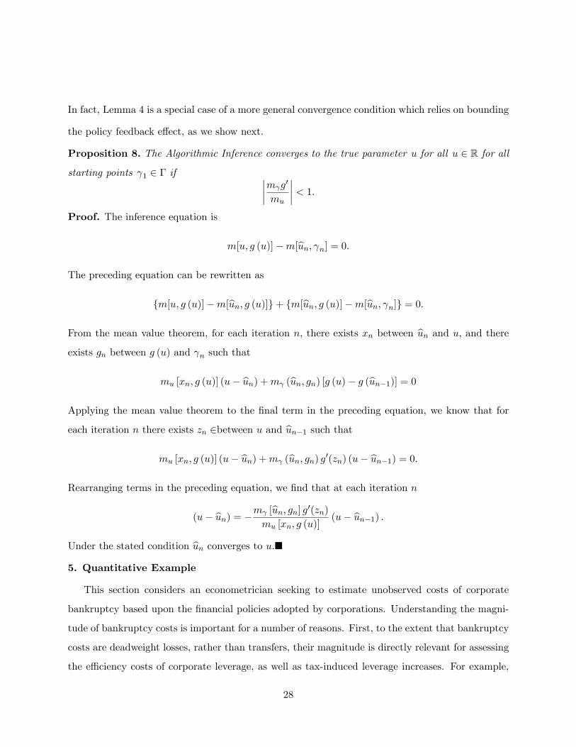
In fact, Lemma 4 is a special case of a more general convergence condition which relies on bounding

the policy feedback effect, as we show next.

Proposition 8. The Algorithmic Inference converges to the true parameter u for all u ∈ R for all

starting points γ1 ∈ Γ if ∣∣∣∣mγg′

mu

∣∣∣∣ < 1.

Proof. The inference equation is

m[u, g (u)]−m[un, γn] = 0.

The preceding equation can be rewritten as

{m[u, g (u)]−m[un, g (u)]}+ {m[un, g (u)]−m[un, γn]} = 0.

From the mean value theorem, for each iteration n, there exists xn between un and u, and there

exists gn between g (u) and γn such that

mu [xn, g (u)] (u− un) +mγ (un, gn) [g (u)− g (un−1)] = 0

Applying the mean value theorem to the final term in the preceding equation, we know that for

each iteration n there exists zn ∈between u and un−1 such that

mu [xn, g (u)] (u− un) +mγ (un, gn) g′(zn) (u− un−1) = 0.

Rearranging terms in the preceding equation, we find that at each iteration n

(u− un) = −mγ [un, gn] g′(zn)

mu [xn, g (u)](u− un−1) .

Under the stated condition un converges to u.�

5. Quantitative Example

This section considers an econometrician seeking to estimate unobserved costs of corporate

bankruptcy based upon the financial policies adopted by corporations. Understanding the magni-

tude of bankruptcy costs is important for a number of reasons. First, to the extent that bankruptcy

costs are deadweight losses, rather than transfers, their magnitude is directly relevant for assessing

the effi ciency costs of corporate leverage, as well as tax-induced leverage increases. For example,

28

in making the case for the Bush Administration Treasury for integration of the individual and

corporate tax systems, Hubbard (1993) contended, “tax-induced distortions in corporations’com-

parisons of nontax advantages and disadvantages of debt entail significant effi ciency costs.”Second,

the magnitude of bankruptcy costs is indirectly relevant to the tax authority estimating revenues.

After all, higher bankruptcy costs serve as a counterweight to tax benefits of debt, discouraging

firms from taking on extremely high leverage. For example, Gruber and Rauh (2007) estimate the

tax elasticity of corporate income is only -0.2, evidence that would appear to contradict Hubbard’s

notion that corporations aggressively change capital structures in response to tax incentives.

Early models, such as that of Stiglitz (1973), failed to deliver interior optimal leverage ratios.

Lacking interior optimal leverage ratios, computational general equilibrium (CGE) models, e.g.

Ballard, et. al (1985), posited exogenous financing rules. In the absence of closed models, public

finance economists such as Gordon and MacKie-Mason (1990) and Nadeau (1993) were forced into

positing ad hoc costs of financial distress. In an important contribution, Leland (1994) showed how

to develop a tractable logically closed model of capital structure for firms facing taxation and costs

of distress using contingent-claims pricing methods.

In this section, we use Leland’s canonical framework to understand the nature of bias that can

arise in careful structural work in a real-world applied policy setting. Consider a government that

is interested in setting the corporate income tax in a way that is optimal according to its objective

function. The magnitude of financial distress costs is clearly relevant here since, as argued above,

the magnitude of these costs determines effi ciency costs of corporate leverage, as well as having a

direct bearing on tax collections.

With this economic setting in mind, consider a structural econometrician who will observe the

financing policies adopted by a set of homogeneous firms funding new investments during the pre-

inference stage.8 Specifically, the econometrician will measure the mean interest coverage ratio,

as measured by the ratio of EBIT to interest expense. As shown below, this moment is directly

informative about bankruptcy costs.

Consider first the decision problem of the firms. Each firm will choose a promised instantaneous

coupon on a consol bond, denoted φ. The firm will use the debt proceeds plus equity injections to

8Firms can have differing EBIT levels. The optimal coupon is linear in EBIT so coverage ratios will be equal

nevertheless.

29

fund a new investment, as is standard in project finance settings. We assume parameters are such

that the investment has positive net present value. Formally, the new investment has positive net

present value if the value of the levered enterprise exceeds the cost of the investment.

Debt enjoys a tax advantage, with interest being a deductible expense on the corporate income

tax return. Consequently, each instant it is alive, the project firm will capture a gross tax shield

equal to φγ, with the random variable γ now representing the corporate income tax rate that

will be implemented just after the econometrician completes her parameter inference. However,

debt service has a negative impact on the firm’s value. In particular, in the event of EBIT being

insuffi cient to service the coupon, the firm’s debt will be cancelled and bondholders will capture

a fraction N(u) of unlevered firm value. The function N here is the standard normal cumulative

distribution function.

Finally, suppose EBIT follows a geometric Brownian motion with drift µ, volatility σ, and initial

value normalized at 1. The risk-free rate is denoted r. The objective is to maximize levered project

value. Or equivalently, firms maximize expected tax shield value minus expected default costs.

Thus, firms solve the following program

maxφ

γφ

(1

r

)(1− φ−λ)−N(u)

φ(1− γ)

r − µ φ−λ. (37)

where λ is the negative root of the following quadratic equation

1

2σ2λ2 +

(µ− 1

2σ2)λ− r = 0. (38)

Note, the first term in the objective function captures tax shield value and the second term captures

bankruptcy costs. Effectively, the tax shield represents an annuity that expires at the first passage

of EBIT to the coupon from above. At this same point in time, bankruptcy costs incurred. This

explains the presence of the term φ−λ in the objective function, which measures the price at date

zero of a so-called primitive claim paying 1 the first passage of EBIT to the coupon from above.

The first-order condition for the optimal coupon entails equating marginal tax benefits with

marginal bankruptcy costs. In particular, the optimal coupon satisfies(γr

)[1− (1− λ)φ−λ] = (1− λ)N(u)

(1− γ)

r − µ φ−λ. (39)

Rearranging terms in the preceding equation, it follows the optimal coupon is

φ∗ = (1− λ)1/λ[1 +N(u)

(1− γ)

r − µr

γ

]1/λ. (40)

30

The moment observed by the econometrician, the mean interest coverage ratio, is 1/φ∗. Thus, in

the present setting

m(u, γ) ≡ E[φ−1] = (1− λ)−1/λ[1 +N(u)

(1− γ)

r − µr

γ

]−1/λ. (41)

Notice, in this particular case,mu(u, γ) > 0 andmγ(u, γ) < 0. That is, the optimal interest coverage

ratio is increasing in bankruptcy costs and decreasing in the tax rate.

Suppose now that the structural econometrician, who recommended the Trump tax cut, failed

to impose the assumption that firms have rational expectations regarding the tax rate. Specifically,

suppose the econometrician treated the tax change as a counterfactual event and parameterized

her model using the status quo tax rate. In the present context, the inference equation (7) takes

the form

m[u, γ∗(u)] = (1− λ)−1/λ[1 +N(u)

[1− γ∗(u)]

r − µr

γ∗(u)

]−1/λ(42)

= (1− λ)−1/λ[1 +N(u)

(1− γ0)r − µ

r

γ0

]−1/λ= m(u, γ0).

Cancelling terms in the preceding equation and solving one obtains

N(u) =[1− γ∗(u)]/γ∗(u)

(1− γ0)/γ0×N(u). (43)

How important quantitatively is the bias implied by the preceding equation? To assess this, we

must stipulate parameter values. Following Goldstein, Ju and Leland (2001) we approximate the

effect of personal taxes by setting γ equal to the Miller (1977) debt tax shield value. In particular, let

γc denote the corporate tax rate, γe denote the equityholder tax rate, and γd denote the debtholder

tax rate. The Miller debt tax shield value is

γ = 1− (1− γc)(1− γe)(1− γd)

. (44)

Goldstein, Ju and Leland (2001) assume γc = 35%, γe = 20% and γd = 35%. These parameter

values are reflective of the status quo before the Trump corporate tax cut, which implies the status

quo policy value is γ0 = 20%. The Trump tax reform cut the corporate income tax rate to γc = 21%.

This tax rate reduction substantially lowered the effective debt tax shield to γ = 2.8%. Substituting

these values into the bias formula in equation (43) we find

N(u) = 8.68×N(u).

31

That is, estimated bankruptcy costs here are 8.68 times actual bankruptcy costs. Intuitively, here

the firms choose low leverage in rational anticipation of the upcoming tax cut. The econometrician

treats the firms as ignorant of the prospective tax cut and treats the low leverage as indicative of

very high bankruptcy costs.

Figure 10 illustrates the cause of the biased inference. The two schedules plot the interest

coverage ratio adopted by firms for alternative values of bankruptcy costs. The schedules differ

according to the assumption adopted in the structural model regarding the tax rate. In one case,

the structural model is predicated upon the assumption that agents expect the status quo to be

maintained. In the other case, agents have a rational expectation of the actual policy change, a

large corporate tax cut, leading them to adopt low leverage. The failure to account for rational ex-

pectations would cause the econometrician to impute the observed low leverage to high bankruptcy

costs.

Such biased parameter estimates will lead to faulty predictions regarding the behavior of firms

after the policy change and a faulty assessment of policy tradeoffs. Continuing to follow the

parameterization of Goldstein, Ju and Leland, assume r = 4.5%, σ = 0.25, µ = 0, and N(u) = 5%.

Evaluated at this parameterization, with the equilibrium γ∗ = 2.8%, equation (40) implies firms

observed during the inference stage will choose coupons equal to 13.63% times initial EBIT(=1).

And note, future generations of firms will adopt this same coupon rate. After all, under rational

expectations, the inference stage firms here will posit the same tax shield value as that which

will actually be operative post-inference. In other words, no reaction will be apparent when one

contrasts the behavior of the inference-stage firms with the behavior of firms post-inference.

The structural econometrician will here mistakenly predict that future generations of firms will

respond to the tax rate change by adopting a much lower coupon rate, failing to understand that

the inference-stage firms already responded rationally to the upcoming change. In particular, based

upon an estimated bankruptcy cost equal to 43.4%(= 8.68×5%), equation (40) leads to a predicted

coupon rate, call it φ, equal to only 1.49% times initial EBIT. However, as shown above, the actual

coupon rate after the tax rate change will be 13.63% times EBIT.

The faulty parameter inference leads to faulty predictions regarding firm behavior after the

policy change which in turn leads to a faulty assessment of policy tradeoffs. To illustrate, note that

the present value of tax collections per firm in this economy is equal to the value of the perpetual

32

stream of taxes on an unlevered entity minus the tax shield value. It follows that the actual and

predicted present value of tax collections are, respectively

T =1− γr − µ − γφ

∗(

1

r

)[1− (φ∗)−λ] = .5546

T =1− γr − µ − γφ

(1

r

)[1− φ−λ] = .6133

That is, the actual present value of tax collections here will be 10.6% lower than predicted tax

collections. Intuitively, the upward bias in estimated bankruptcy costs leads to a faulty prediction

of low leverage leading to a faulty prediction of high corporate income tax collections.

Conclusion

An asserted advantage of moment-based structural microeconometrics over reduced-form meth-

ods is that one can correctly identify policy-invariant parameters so that alternative policy options

can be assessed. As we have shown, this approach, which generally treats policy changes as coun-

terfactual zero probability events, violates rational expectations: agents inside the structural model

should understand that policy changes are positive probability events which the econometric exer-

cise in intended to inform. We examined the implications of this violation of rational expectations

in moment-based microeconometric parameter inference which serves a policy function. As shown,

bias emerges unless the true value of the parameter justifies the status quo. If instead a policy

change is justified, biased inference occurs. Finally, it was shown how rational expectations can be

imposed in an internally consistent manner, yielding unbiased inference and optimal policy.

33

References

[1] Ballard, C.L., Shoven, J.B. and Whalley, J., 1985. General equilibrium computations of the

marginal welfare costs of taxes in the United States. The American Economic Review, 75(1),

pp.128-138.

[2] Blanchard, O. and Portugal, P., 2001. What hides behind an unemployment rate: comparing

Portuguese and US labor markets. American Economic Review, 91(1), pp.187-207.

[3] Blume, L., Easley, D. and O’Hara, M., 1982. Characterization of optimal plans in stochastic

dynamic programs, Journal of Economic Theory 28, 221-234.

[4] Chintagunta, P., Erdem, T., Rossi, P. and Wedel, M., 2006, Structural models in marketing.

Marketing Science 25 (6), 551-600.

[5] Ejarque, J. and Portugal, P., 2007. Labor adjustment costs in a panel of establishments: a

structural approach.

[6] Gallant, A.R. and Tauchen, G., 1996. Which moments to match?. Econometric Theory, 12(4),

pp.657-681.

[7] Goldstein, R., Ju, N. and Leland, H., 2001. An EBIT-based model of dynamic capital structure.

The Journal of Business, 74(4), pp.483-512.

[8] Gomes, J.F., 2001. Financing investment. American Economic Review, 91(5), pp.1263-1285.

[9] Gordon, R.H. and MacKie-Mason, J.K., 1994. Tax distortions to the choice of organizational

form. Journal of Public Economics, 55(2), pp.279-306.

[10] Gruber, J. and Rauh, J., 2007. How elastic is the corporate income tax base?. Taxing corporate

income in the 21st century, pp.140-163.

[11] Hamermesh, D.S., 1989. What do we know about worker displacement in the US?. Industrial

Relations: A Journal of Economy and Society, 28(1), pp.51-59.

[12] Heckman, J.J., 2000. Causal parameters and policy analysis in economics: A twentieth century

retrospective. The Quarterly Journal of Economics, 115(1), pp.45-97.

34

[13] Hubbard, R.G., 1993, Corporate tax integration: A view from the Treasury Department.

Journal of Economic Perspectives 7, 115-132.

[14] Kahn, R. and Whited, T.M., 2017. Identification is not causality, and vice versa. The Review

of Corporate Finance Studies.

[15] Keane, Michael P., 2010, Structural versus atheoretic approaches to econometrics, Journal of

Econometrics 156, 1-21.

[16] Leland H., 1994, Corporate debt value, bond covenants, and optimal capital structure, Journal

of Finance.

[17] Miller, M.H., 1977. Debt and taxes. the Journal of Finance, 32(2), pp.261-275.

[18] Nadeau, S., 1988, A model to measure the effect of taxes on the real and financial decisions of

the firm. National Tax Journal 41, 467-481.

[19] Rust, John, 2010, Comment on structural versus atheoretic approaches to econometrics, Jour-

nal of Econometrics 156, 21-30.

[20] Sargent, T.J., 1984. Autoregressions, expectations, and advice. The American Economic Re-

view, 74(2), pp.408-415.

[21] Sargent, T.J., 1987. Rational Expectations. The New Pelgrave, Eatwell, Murray and Newman

Editors, London.

[22] Sent, E.M., 2006. The evolving rationality of rational expectations: An assessment of Thomas

Sargent’s achievements. Cambridge University Press.

[23] Sims, Christopher A., 1982, Policy analysis with econometric models, Brookings Papers on

Economic Activity 1, 107-164.

[24] Stiglitz, J.E., 1973. Taxation, corporate financial policy, and the cost of capital. Journal of

Public Economics, 2(1), pp.1-34.

[25] Wolpin, K., 2013, The limits of inference without theory, MIT Press.

35