Equilibrium Federal Impotence

Equilibrium Federal Impotence: Why the States and Not the American NationalGovernment Financed Economic Development in the Antebellum Era

John Joseph Wallis and Barry R. Weingast

March 2005

Professor, Department of Economics, University of Maryland and Research Associate, NationalBureau if Economic Research; and Senior Fellow, Hoover Institution, and Ward C. KrebsFamily Professor, Department of Political Science, Stanford University. This research wasundertaken while Wallis was a National Fellow at the Hoover Institution whose generoussupport is acknowledged. The authors gratefully acknowledge Daniel Carpenter, Brad DeLong,Martha Derthick, Morris Fiorina, Douglas Grob, Michael Holt, Gary Libecap, Douglass North,Wally Oates, Christina Romer, Kenneth Shepsle, Richard Steckel, Steve Usselman, RichardWhite, and seminars at the NBER Development of the American Economy program meeting andthe 2004 EHA meetings for helpful conversations.

1Federal Impotence

1. Introduction

American governments devoted substantial resources to promoting economic development

before the Civil War. The United States was an agrarian economy with millions of acres of

virgin land. Economic growth required investment in transportation (roads, canals, and

railroads) to open frontier land to markets and in banks to finance shipment of goods to markets.

Governments financed both financial institutions and large-scale internal improvements

(Callender 1903, Goodrich 1960, North 1966, Taylor 1968, Larson 2001).

The puzzle is that state, not the national, governments played the central role as promoters of

development. Indeed, state financial efforts were nearly an order of magnitude larger than the

federal government’s. Between 1790 and 1860, the federal government spent $60 million on

transportation improvements, while state and local governments spent over $450 million. Every

American is a citizen of both a state and the United States. Given the demand for public goods to

promote development, why did the states and not the national government supply these public

goods?

Several other aspects of early America make the contrast more puzzling. First, the national

government should be more efficient provider of infrastructure. The nation whole is better able

to spread the risks of such an investment than an individual state, an explanation often used to

justify the modern leadership of the national government in economic policy. Second, the

national government typically ran a budget surplus in peacetime before 1860, so fiscal

2Wallis and Weingast

1Federal government finances were tight during the 1790s and during the War of 1812. In1815 the national debt was $137 million; by 1835 it was paid off completely. In the 1820s,annual federal revenues averaged $22 million and expenditures only $16; in the 1830s, $30million and $24 million. Historical Statistics of the United States.

constraints played a limited role in the national government’s failure to provide these market-

enhancing public goods.1

Our specific puzzle is related to a third issue. The national Constitution created a

government of limited powers, including a strong system of federalism, a system that pitted

“ambition against ambition.” Did the incentives facing public officials limit their ability to

exercise political power?

To address these questions, we model the political economy of a legislature facing the choice

of funding a large infrastructure investment. The model has three related results. First, the

political constraints inherent in majority rule prevented the federal government from financing

large infrastructure projects. Large projects provided geographically highly concentrated benefits

with diffuse costs. Because such projects made most areas of the country worse off, they could

not command a majority of votes. Although logrolling was possible, in practice the scale of

infrastructure investments like the Erie Canal limited logrolling because only a few could be

built at once.

Second, two separate political forces pushed Congress toward financing large collections of

smaller projects – such as lighthouses, roads, or dredging harbors – distributed across the entire

country. We term these large collections “universalism,” or “something for everyone.”

Coalitional politics push toward universalism (Weingast 1979). When members of Congress are

uncertain about what winning coalition that will form, a universal coalition provides higher

3Federal Impotence

expected returns to each district and its representative than narrower majority coalitions. The

second force, the exit constraint -- the idea that states would leave the Union if federal policies

left them significantly worse off -- also pushed toward universalism. As we note below, exit was

a serious threat in early America: southern states seceded in 1861. The exit constraint implies

that narrow majority coalitions, especially regional ones, risk secession by the areas locked out

of power. Universalism emerged as the natural solution to both the majority constraint and the

exit constraint.

Third, we show that benefit, or Lindahl, taxation provided another solution to these political

constraints. If the government can tax each locality or state in proportion to the benefits it

receives from the project, then regions outside the area benefitting from the project pay no taxes

and so will not oppose it. The Constitution prohibits the federal government – but not the states –

from using benefit taxation to finance projects: it requires that federal direct taxes be assessed

among the states on the basis of population.

These results explain the puzzles noted above. The state and national governments

persistently financed development projects in different ways. The Constitutional prohibition on

benefit taxation combines with the logic of congressional politics to imply that the federal

government could not finance large projects. To the extent that the national government financed

transportation investment, it did so through something for everyone programs. In contrast, states

financed large projects using benefit taxes, assessing property owners in proportion to their

expected economic gains from the new project. This mechanism allowed them to solve the same

political problems that plagued the national government.


Finally, these results bear on our larger question about the incentives for how the national

government observed limits on its power in early America. The Constitution created a series of

political constraints that made it politically impossible for the federal government to finance

large infrastructure projects. Federal efforts came either in form of financing large collections of

small projects or formal allocation formulas to distribute funds to every state. In short, the

national government was politically impotent with respect to the provision of the highest valued

infrastructure projects.

Section 2 of the paper develops the theory of legislative choice and derives our results about

state and federal policy decisions. Sections 3 and 4 apply these results to the antebellum era’s

national and state programs to finance economic development. Sections 5 and 6 consider federal

policy in more detail.

2. A Theory of Legislative Choice and Infrastructure Investment

We turn to the theory of legislative choice to understand the three phenomena to be explained:

the federal government’s inability to promote economic development through financing large

infrastructure projects; its ability to finance many small projects; and why the states were not

plagued by the same problems.

Today we think of the president as the national leader, the source of most major legislative

initiatives. Yet this is a product of the twentieth century. In the nineteenth century, Congress

was at the center stage of national legislation. All the famous compromises that revised aspects

5Federal Impotence

2This discuss draws on modern theories of congressional decisionmaking, particularly ina historical context. See, e.g., Aldrich (1995), Cox and McCubbins (1993,2005), Krehbiel(1994), Polsby (2004), Rohde (1991), Schickler (2001), Stewart (2001), Shepsle (1989),Weingast and Marshall (1988).

3In what follows, we adapt the models in Inman (1988), Shepsle and Weingast (1984) andWeingast, Shepsle, and Johnsen (1981).

of the American national framework and helped sustain the United States were negotiated and

written in Congress, including those of 1820, 1833, 1850, and 1877.

We consider those nineteenth century policies which sought to spend revenue to build

transportation links: roads, canals and, later, railroads, as wells as rivers and harbors projects and

lighthouses. The model applies to both the American federal and state governments, so we talk

about generic legislatures and districts, rather than states, districts, or counties. Both Congress

and state legislatures are geographically oriented.2 Because legislators are elected from specific

geographic constituencies their electoral incentives force them to concern themselves about the

incidence of policies on their district. Although national or statewide interests matter, it is

primarily the effects of policies on their district that determine whether a given member favors a

policy (Stewart 2002).

Consider an expenditure policy to provide a public good, π(x) = (P1(x), P2(x), ... , Pn(x))

where n is the number of districts, π(x) is a public policy, and the Pi(x) represent the incidence of

the policy on district i.3 The various functions are written as a function of x, a scale factor that

reflects the size of the policy.

Pi(x) can be broken into the benefits, bi(x), and costs, ci(x), where Pi(x) = bi(x) - ci(x). We

assume that the benefits are concave and the costs are convex as a function of x; that is, biN> 0,

biO<0, and ciN>0 and ciO > 0 œi.


4For simplicity, we treat all costs as tax costs, but clearly the costs and benefits toconstituents and legislators can come in many forms.

5Each legislator i has an ideal policy of xi* which solves the problem max Pi(x) andwhich occurs when the marginal benefits to district i equals the districts costs, i.e., biN(x) =tiCN(x).

6All voting models require an assumption about what happens when a legislator isindifferent between two alternatives.

The total net social benefits for the state is represented as:

Z(x) = 3i Pi(x) = 3i (bi(x) - ci(x)).

The economically efficient policy, x*, is such that at x*, ZN = 0 and ZO < 0 so that at x* the

marginal net social benefits are zero; i.e., 3i (biN(x) - ciN(x)) = 0. Legislative outcomes are

unlikely to meet this criteria, however.

Let C = 3i ci(x) be the total costs of the project, and let T be the total taxes needed to finance

the project. We assume a balanced budget constraints, so that T = C. Further, district i’s tax

share is ti, so that its tax cost for a particular project is tiC.4

District i’s legislator’s objective function is Pi(x) = bi(x) - tiC(x).5 Legislators consult only

their own objective function, ignoring the effects of the project on other districts, and hence the

project’s social implications. When choosing between two projects, or between building a

particular project and not, each legislator supports the alternative that provides higher net

benefits. Moreover, we assume a convention about indifference: if a legislator’s district bears no

costs for a project, she votes in favor even if her district receives no benefits.6 It is clearly

costless for such a legislator to do so.

7Federal Impotence

7Given a single dimensional policy choice, such as the choice over the scale of a singleproject, the majority rule equilibrium is the ideal policy of the median district. Standard resultsshow that, except in very special circumstances, no majority rule equilibrium exists when thelegislature chooses the scale of many projects simultaneously. These concepts are defined inHinich and Munger (1997), Shepsle and Bonchek (1997), and Stewart (2002).

8Schlesinger (1922) shows that every state had some secessionist movement prior to theCivil War. See Hendrickson (2003) for a recent treatment of forces leading to disunion in theearly nation.

Legislatures are constrained in two ways. First, passage of individual legislation is only

possible if a majority of legislators benefit from the proposed legislation.7 This majority rule

constraint applies to individual pieces of legislation. Logrolling makes it possible to fund

individual projects (as opposed to legislation) that benefit a minority of legislators, as long as the

project is paired with enough other projects that a majority of legislators receive positive net

benefits from the entire package. For simplicity, the majority rule constraint requires that all of

the necessary logrolls be bundled into one bill.

Second, the exit constraint applies to the aggregate of all legislation passed by the

legislature. At the national level, every state must receive positive net benefits from the sum of

all legislation passed, or it “exits.” The exit constraint requires that no district is hurt, on balance,

by the aggregate actions of the government. Threats of exit were common in the early United

States. Threats to secede or dramatically weaken the union occurred with the Virginia and

Kentucky Resolutions (1798), the Hartford Convention (1815), the Nullification Crisis (1832-

33), and the sectional crises of 1819-20 (over Missouri), 1846-50 (over the Mexican Cession),

and 1854-61 (following the Kansas-Nebraska Act), which resulted in the Civil War.8

The exit constraint requires that:

'IPij(x) > 0 (summed over j policies, œi ).


We will return to consider the historical relevance of both the majority and the exit constraint

later. With respect to states, mobile factors of capital and labor will leave the state if some

region is a permanent minority that receives too little benefits in comparisons with its taxes.

The legislature must make simultaneous decisions about the size of the project, the

allocation of benefits across districts, and the allocation of tax burdens across districts. We

characterize legislative outcomes under four different mechanisms of public finance: normal

taxation, benefit taxation, universalism or something for everyone, and taxless finance. These

categories are not mutually exclusive, nor are they exhaustive, but they give us a framework to

discuss the choice set facing Congress and the state legislatures in the early 19th century. We

continue to consider one big project, like the Erie canal.

A. One large project: Normal taxation. Normal taxes are the general revenue

instruments already in use by the government. In the case of the federal government in the early

19th century, financing expenditures by normal taxation involved revenue from import duties, the

national government’s principal tax.

Large projects have several relevant characteristics. First, they require very large

expenditure relative to the budget, implying that at most only one or two such projects can be

built at once. Second, these projects concentrate the benefits in a small geographic area while

spreading the tax costs across the entire polity. This implies that some districts receive large

benefits relative to their tax cost: bi(x*) > tiC(x*); but many districts receive no benefits while

bearing their tax cost: Pi(x) < 0 œx>0, since bi(x) = 0 while tiC(x) > 0.

The concentration of benefits in a few districts implies that most districts pay taxes while

receiving no benefits. These districts both naturally oppose the project and comprise a majority,

9Federal Impotence

9To see that bi > tiC under benefit taxation, substitute on the right hand side: tiC = (bi/B)C= (C/B)bi. Since C/B < 1, the first inequality holds.

so the majority rule constraint implies that no project is built. The size of the project makes it

impossible to find enough logrolling options to compensate districts that do not gain from the

large project. Even if it is possible to find a project that benefits a majority of districts, a simple

majority fails to meet the exit constraint. In short, it is difficult for government to build a large,

expensive, geographically concentrated project through normal taxation.

B. One large project: Benefit taxation. The first result assumed that the financial costs of

the project were spread across the state through general taxation. Suppose instead that the project

could be financed by a tax scheme, benefit taxes, also known as Lindahl taxes. In this scheme,

district i’s tax share is a function of the benefits it receives from the project.

Let the B(x) = 3i bi(x) be the project’s total benefits. Define a benefit taxation scheme so that

ti = bi/B. Under this tax scheme, districts that receive no benefits from the project also pay no

taxes regardless of the project’s total cost: bi = 0 implies that ti = 0/B = 0. Districts pay their

share in taxes in proportion to the benefits they receive.

As long as the project’s total benefits exceed the total costs (B > C), each district with

positive benefits also has positive net benefits after paying their tax share.9 Thus, assuming that

representatives who are indifferent to the project – including legislators whose districts receive

no benefits but also incur no costs – vote in favor of the project, every legislator (weakly) favors

the project, so it will pass. In contrast to the case where projects are financed out of general

revenue, benefit taxation implies that, even in the case of a large project like the Erie canal, most

districts receive no benefits and incur no costs, and so they can costlessly support the project.


10The federal government levied a property tax in 1799, 1814, and 1862, but the tax hadto be allocated between states on the basis of population, it could not be allocated on the basis ofbenefits as measured in increased wealth or property values.

11Taxless finance is considered in greater detail in Wallis, 2005, “Constitutions,Corporations, and Corruption.”

12Canals required eminent domain and banks required limited liability and, often, theprivilege of note issue.

The widespread use of the property tax provided states with a potential mechanism for

creating a benefit tax. When the value of transportation improvements is capitalized in land

values and property taxes are used to fund construction, it is possible for every district to, at

worst, be indifferent to the large project. The use of benefit taxation to finance a single large

project simultaneously satisfies the majority and exit constraints.

The central problem with a single large project is the inability to balance off the losses to

districts that do not benefit from the project because the state is unable to afford multiple large

projects. Benefit taxation solves that problem. The Constitution explicitly prohibited the federal

government from using benefit taxation: “Representation and direct taxes shall be apportioned

among the several States which may be included in this Union, according to their respective

Numbers...” (Article 1, Section 2).10

C. One large project: Taxless finance. There are several alternatives to financing a project

through taxes. These financing schemes share a common element: building the project does not

entail raising current taxes, thus taxless finance.11 Suppose the canal is expected to generate a

stream of toll revenues, but its construction requires government assistance in the form of

eminent domain, limited liability, and financial assistance.12 The government could charter a

company, creating the special privileges, and then use the good faith and credit of the

11Federal Impotence

13The second taxless finance variant was commonly used to finance state investments inbanks.

government to secure operating capital by issuing bonds. The government then invests the

borrowed funds in the private corporation by purchasing stock. Dividends from the

government’s investment are expected cover the government’s interests costs. Taxpayer’s

liability in this case were contingent on the success of the project. If the project succeeded, the

government received a steady flow of dividends, net of interest costs, allowing it to lower taxes.

If the project failed, the government and its taxpayers would assume the debt service.13 The First

and Second Banks of the United States were financed in this manner.

A second method of taxless finance was used extensively by the federal government: land

grants. In these schemes, the federal government would give project promoters grants of federal

land, in alternating strips along the right of way. Project promoters could sell their land to raise

funds. Federal lands were an important source of federal revenue, and the idea was that

taxpayers would gain from the grant by raising land values on the land the federal government

did not give away. The rise in land values would offset the loss of land revenue from the grant.

Federal land values had to more than double for this to happen. Grants were made to Ohio,

Indiana, and Illinois in the 1820s, and the Union and Central Pacific Railroads in the 1860s.

Taxless finance works politically because of the implicit benefit received by all districts.

Current taxes may not rise, but taxpayers do assume an expected, contingent liability:

CLi = tiC(x)(1-s)


14By 1830, states were able to draw on 40 years of experience with investment in banks,with the expectation that “M” was positive and large, and that the probability of a successfulinvestment, “s,” was close to one. Canal investments in New York and Ohio had also provenprofitable. Governor Ford of Illinois, spoke directly to the ex ante expectations of the Illinoispoliticians when he explained how the state got itself into difficulties in his message to thelegislature of December 8, 1842 “No scheme was so extravagant as not to appear plausible tosome. The most wild expectations were made of the advantages of a system of internalimprovements, of the resources of the State to meet all expenditures, and of our final ability topay all indebtedness without taxation. Mere possibilities appeared to be highly probable, andprobabilities wore the livery of certainty itself.” Quoted in House Document, p. 1051.

where s is the ex ante probability of project success. If the project fails ex post, CLi will be

positive for all districts. Note that Pi(x) is negative for any districts who receive no immediate

benefits, i.e. for whom bi(x) = 0.

A taxless finance scheme that does not provide benefits to all districts, ex ante, will have a

negative expected value to a majority of districts and will not be supported:

Pi(x) = bi(x) - tiC(x)(1-s) < 0 (œi where bi(x) = 0).

Taxless finance does not work that way, however. The assumption is that the project will

return money to the treasury, either in the form of dividends on the government’s stock or higher

revenues from land sales. If M represents the potential profit of the enterprise to the

government, then the calculation of net benefits for each district becomes:

Pi(x) = bi(x) + tiM(s) - tiC(x)(1-s).

That is, each district expects its taxes to go down by tiM if the project is successful. The critical

issue for districts who do not benefit directly from the canal, districts where bi(x) = 0, is whether

tiM(s) >< tiC(x)(1-s). Taxless finance works politically because it promises every district that its

taxes will be lower if the project succeeds.14 Of course, a major element in whether these

13Federal Impotence

15This subsection draws on the large literature on universalism, including Collie (1988),Inman and Fitts (1990), Niou and Ordeshook (1985), Shepsle and Weingast (1981), Stein andBickers (1995), and Weingast (1979).

16 Both of these restrictions are easily generalized, for example, to projects that benefit asmall number of (perhaps contiguous) districts simultaneously.

17All of these assumptions can easily be generalized, so that the benefits, bi, costs, ci, andtax share, ti, differ across districts.

schemes are perceived by citizens to have positive expected value depends on s, the probability

of success.

As with benefit taxation, taxless finance can simultaneously satisfy the majority constraint

and the exit constraint.

D. Many projects: Universalism or Something for Everyone. We emphasize the financing

of a single large project because of its relevance for state transportation investments in the

antebellum era. But the provision of small transportation projects was also relevant for federal

investment. Many antebellum expenditure policies fell into this category, rivers and harbors

projects, lighthouses, post offices, and roads.

Two separate political forces push the legislature toward universal or something for

everyone solutions. Consider a legislature facing decisions over a range of projects, each with

concentrated local benefits and paid for through general taxation.15 For simplicity, we assume

that each legislator has one proposed project; and that each project benefits her district and her

district alone.16 Moreover, assume that each project is small relative to the budget, so that there is

no problem financing many or all at the same time. Let the benefits to each district from its

project be b; that these are identical across districts, as are all the costs, c; and that each district

pays an equal tax share of 1/n of the total costs.17


18Buchanan and Tulloch (1962) and Riker (1962) initiated the application of MWC’s tolegislatures.

Legislators now consider bundles of projects. Given each legislator’s preferences, the ideal

bundle of projects is simple to characterize. Each legislator receives positive benefits only if the

project for her district is built. Building any or all other projects merely raises the district’s taxes.

So each legislator’s ideal policy is to build her project alone. Unfortunately any legislation of

that type will be defeated by a vote of n-1 to 1, with only the legislator benefitting voting in

favor. Legislators therefore have an incentive to create bundles of projects though logrolling.

The literature has studied two natural types of bundles or logrolls. The first is a minimum

winning coalition (MWC) whereby (n+1)/2 legislators build their projects alone.18 For those

legislators whose projects are built, this maximizes their net benefits. Enlarging the coalition

gains votes beyond the minimum needed. Yet, because it raises each coalition-members taxes

without increase their benefits, each is worse off. Of course, those legislators not included in the

MWC are worse off since their projects are not built, but they pay their share of the taxes to

finance the MWC’s projects. This implies that, once a given MWC forms, it is hard to overturn:

all members of the coalition benefit from this bundle; no bundle makes them better off; and they

are better off than if no projects are built.

The problem is that there are too many such coalitions, and ex ante no legislator is assured of

being in the MWC so that their projects will be built. Thus, MWC politics involves risk.

As an alternative, the legislature might institute and enforce a policy of universalism, the

notion that rather than play MWC politics, the legislature will simply build a project for each

district. Various “universalism theorems” show that, in comparison to the uncertainty of MWC

15Federal Impotence

19One potential qualification of universalism that we ignore here is that universalism mayapply within majority party only, so that projects are not built in districts represented by theminority party.

politics that build fewer projects than one for each district (but at least a majority), every

legislator is better off under universalism (Niou and Ordeshook 1985, Shepsle and Weingast

1981, Weingast 1979).19

Although the proofs of these results are a bit technical, the intuition is straightforward. For

simplicity, suppose that the benefits to each district, b, are identical, as are all the costs, c; and

that each district pays an equal tax share of 1/n of the total costs. Under the MWC politics,

legislators whose projects are built receive the benefits from their project, b, minus their share of

the tax costs of c(n+1)/2. As n becomes large, the size of the minimum winning coalition

approaches ½ of the legislature, so we will approximate the MWC tax share as one half; that is,

c/2. Further, since no one knows which MWC will form, we consider each equally likely. This

implies that a given legislator’s chances of being in the MWC that forms is on the order of one

half.

Thus, ex ante, each legislator’s expected value of the uncertain MWC politics is 1/2[b - c/2]

(when district i’s project is built)+ ½(-c/2) (when district i’s project is not built). Rearranging

terms, the expected value of MWC politics is 1/2[b - c/2] + ½(-c/2) = (b-c)/2. In contrast, under

universalism, each district is assured its project, so the expected benefits are b-c. Because b-c

exceeds (b-c)/2 (as long as b-c > 0), all legislators prefer to institute and maintain a set of

institutions providing for universalism.

The universalism result shows that national expenditure programs can pass that provide large

numbers of small projects, located across the country.


A second result concerns parties. if the coalitional structure is known in advance – e.g., a

majority party or a region – then restricting universalism to that coalition provides its members

with greater individual benefits to the party’s members. Whether this happens depends on the

geographic distribution of the majority party. If it is geographically concentrated, so that the

minority is also geographically concentrated, financing the projects solely of majority party

members is likely to violate the exit constraint.

The main point is that, when the legislature seeks to build large numbers of small projects,

the tendency is toward universalism. We discussed two variants: with and without a majority

party. Without a majority party, universalism is likely to hold. With a majority party, the oucome

depends on geographic concentration. Without concentration, then majority party is likely to

build projects solely for its members; but with concentration, doing so violates the exit

constraint. If the exit constraint binds, majority parties are constrained from excluding the

minority party.

Another variant on this solution is, in contrast to building projects, the legislature might

choose to simply provide funds to lower jurisdictions (e.g., grants by the Congress to the states;

grants by state legislatures to counties or towns). Suppose that spending is allocated among

districts by some formula or rule of thumb (such as equal grants per capita). Grant shares to

individual districts are given by gi

Pi(x) = bi(gix) - tiC(x).

Further suppose that at an arbitrarily small amount of spending, ε, produces net benefits for all

districts:

Pi(ε) = bi(giε) - tiC(ε) > 0 œi.

17Federal Impotence

Now the only problem facing the legislature is how much to spend. If the exit constraint is

binding, expenditures will increase until the first district receives no net benefits. If the exit

constraint can be eased by logrolling, then expenditures can increase further.

A simple virtue of something for everyone policies is that the same formula can often be

used to allocate taxation and expenditures. For example, the constitution constrains the federal

government to allocate direct taxes according to population. Direct taxes could be raised to

finance expenditures and funds could be divided between states according to population. It is

important to note, however, that the ti and gi need not be the same. They only need to be known.

E. Predictions about Legislative Choices. Governments could finance investments in

transportation in four ways. Building a canal with limited geographic benefits was politically

infeasible using normal taxation. Too many geographic interests obtained nothing except the

prospect of higher taxes. Building transportation infrastructure with something for everyone

policies was politically feasible, but fiscally impossible if the projects were large. New York

could not afford to build an Erie Canal to every county. Universalist or something for everyone

policies required equal, or close to equal, allocation of funds to every district. Small projects

were politically feasible, but in the end did not develop an interregional transportation system.

A large canal investment could be made with benefit taxation or taxless finance. Benefit

taxation worked very differently from taxless finance, however. Benefit taxation required that

taxes be raised simultaneously with the onset of construction and borrowing. Taxless finance

allowed taxpayers to assume a contingent tax liability, one that would only be assumed in the

event the project failed. Both benefit taxation and taxless finance held out the promise of


20Benefit taxation and taxless finance were not mutually exclusive policies, a state coulduse a little of each. Both benefit taxation and taxless finance legislation were easier to pass whenthere were large expected returns from the project.

significant benefits.20 The constitutional restrictions placed on federal direct taxation made it

difficult, if not impossible, for the federal government to use benefit taxation.

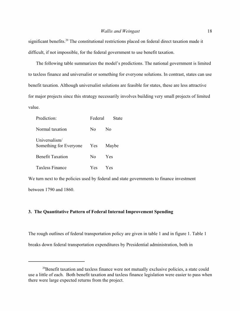
The following table summarizes the model’s predictions. The national government is limited

to taxless finance and universalist or something for everyone solutions. In contrast, states can use

benefit taxation. Although universalist solutions are feasible for states, these are less attractive

for major projects since this strategy necessarily involves building very small projects of limited

value.

Prediction: Federal State

Normal taxation No No

Universalism/ Something for Everyone Yes Maybe

Benefit Taxation No Yes

Taxless Finance Yes Yes

We turn next to the policies used by federal and state governments to finance investment

between 1790 and 1860.

3. The Quantitative Pattern of Federal Internal Improvement Spending

The rough outlines of federal transportation policy are given in table 1 and in figure 1. Table 1

breaks down federal transportation expenditures by Presidential administration, both in

19Federal Impotence

aggregate and per capita terms. Figure 1 provides nominal federal transportation expenditures

per capita, per year from 1790 to 1860 as well as transportation expenditures as a share of total

federal expenditures.

The federal government spent money on transportation in every year in the early 19th century

and every Congress considered transportation legislation. As Figure 1 shows, nominal

expenditures rose slowly from 1790 through the 1810s, stalled during the early 1820s, rose

rapidly to a peak in 1837, dropped back sharply to their 1810s levels, then rose again in the

1850s. The picture is one of very small expenditures with only one significant expansion during

the administration of Andrew Jackson. Nominal per capita income in 1840 was roughly $100, so

federal transportation expenditures in their highest year were only .1 percent of national income,

and were typically on the order of .01 percent of national income. The federal government

steadily spent a small amount of money on lighthouses, navigation improvements, and rural

roads. Beyond that the federal government did very little.

Assessing the model’s predictions

Our theoretical framework identifies four ways the federal government could have used to

finance internal improvements. Table 2 compares the model’s predictions about each method of

finance with the amounts actually spent by the federal government. The main prediction is that

the federal government will not finance transportation projects with normal taxation or benefit

taxation, but will use taxless finance and universalism or something for everyone. The

prediction is borne out. In total, 97 percent of all federal transportation expenditures were

financed in using these two methods.


21The largest single federal project, aside from the Cumberland Road, was the Delawarebreakwater, which received $2.1 million in total. The breakwater funding was appropriatedpiecemeal, however, through rivers and harbors legislation.

The federal government used universalistic something for everyone schemes to finance 68

percent of its infrastructure expenditures. Rivers and Harbors bills were the main legislative

vehicle for funding these improvements. All the projects were small, and as was usually the case,

individual bills embodied logrolling within one piece of legislation.21 The national government

financed another 28 percent of expenditures with taxless finance. Most of the taxless finance

schemes used public land and are discussed in detail below.

We now consider the different federal policies related to financing internal improvements

and related programs.

Something for Everyone. Expenditures for lighthouses, roads, navigation, and general

rivers and harbors accounts for the lion’s share of expenditures made by the federal government

between 1790 and 1860: $41,435,000 out of $60,152,000.

Normal taxation. Financing transportation expenditures through normal taxation was

possible. In the Monroe and Adams administration, Congress appropriated funds to purchase

stock in the Chesapeake and Delaware and Chesapeake and Ohio canals, as well as other smaller

canals. Table 2 credits the $1,917,000 for these canals entirely to normal taxation; about three

percent of federal spending during the antebellum era. Normal taxation was possible, it just did

not amount to much.

Benefit Taxation. Benefit taxation was prohibited by the Constitution and was not used.

Taxless Finance. Taxless finance includes land grants and other projects. Land grants

came in two forms. One was land funds, in which a percentage of all revenue from federal land

21Federal Impotence

22Gates, 1968 and JEH article, 19??.

sales in public land states to those states was dedicated to building transportation projects to and

within those state. The Cumberland Road stretched from Washington D.C. to Illinois and was

the largest single federal project. The Road was initiated by the Enabling Act for Ohio in 1802,

which set aside 2 percent of land sales revenues in Ohio to build roads to Ohio. Similar funds

were established for other public land states (discussed in detail later). The second form of

taxless finance using public lands were the direct grants of land to states like Indiana and Illinois

for support of their canals.

In the table, land grants included the land given to states (valued at $1.25 an acre), the

revenues from the land funds created in state enabling acts transferred to the states, and the

expenditures on the Cumberland Road. The motivation behind land funds and outright grants to

new states was explicitly fiscal. Land grant schemes were predicated on the expectation that the

value of public land near the improvement would rise if transportation to an in the west

improved. Land grant schemes illustrate the theoretical point that such ventures include a

contingent form of liability. Land grants turned out, ex post, to cost federal taxpayers lost land

revenues. Transportation improvements did raise land values, but higher land values did not

translate into higher sale prices at federal land auctions after 1820.22

Congress also used taxless finance in other ventures. In 1791 and 1816, the federal

government chartered national banks. The First Bank was chartered with a capital of $10 million

of which the government subscribed $2 million. The Second Bank was chartered with a capital

of $35 million of which the government subscribed $7 million. In both cases, the government

paid for its stock by issuing federal bonds to the banks (private subscribers could pay in specie or


23The land was given in alternating one-square mile sections, in a strip ten miles to eitherside of the road. Land was transferred to the company after it completed each 40 mile longsection of track. Section 3, An Act to Aid the Construction of a Railroad, 37th Congress, 2ndSession, Chapter 120.

24 Section 5, An Act to Aid the Construction of a Railroad, 37th Congress, 2nds Session,Chapter 120.

federal bonds). The banks paid dividends semi-annually, and the dividends paid to the federal

government for its stock always exceeded the interest payments on the bonds the federal

government used to purchase stock. This illustrates the principle of taxless finance: no taxpayer

paid higher taxes because of the federal government investment in either Bank of the United

States.

In 1862, the Union Pacific Railroad combined two forms of taxless finance, land grants and

bond issues. The company’s charter promised to give the railroad ten square miles of public

land for every mile of railroad the company completed.23 In addition, the federal government

would give the company $16,000 in federal bonds for every mile of track completed. The bonds

were an “ipso factor ... first mortgage on the whole line of the railroad and telegraph.” The

company was responsible for servicing the bonds and repaying the principle.24 Tax payers were

not supposed to pay to service the bonds, and the value of federal lands were supposed to

increase enough to outweigh the substantial acreage given to the railroad. The twists and turns

of the Union Pacific are too complicated for us to follow. Suffice it to say in the end the federal

government regretted that it had used taxless finance in this particular scheme.

23Federal Impotence

25As noted earlier, we derive our $60 million estimate from Senate Executive Document190, 42nd Congress, 1st Session. The $450 million figure for state and local expenditure is aestimate made by Goodrich, Government Promotion. There is no breakdown on the total $450million that we can analyze by financing type.

4. State Investment in Internal Improvements

As noted, state investment in transportation outstripped federal investment by an order of

magnitude. Goodrich estimates that state and local expenditures for transportation were a

combined $450 million before the Civil War, while federal government expenditures were $60

million (Table 1).25

State budgetary data for the antebellum era are problematic and full accounting of state

expenditures by function is not possible [Wallis, 2000]. One way to characterize state financial

activity is to classify state debt outstanding in 1841 by type of financial method. The $198

million outstanding in 1841 came just at the end of the dramatic expansion of state investment in

canals, railroads, and banks in the 1830s. Since states faced the same political constraints as the

federal government -- a democratic legislature attempting to build geographically concentrated

projects to satisfy geographically diverse constituencies – we expect to see the same pattern of

outcomes with two differences. One, states are not prevented from using benefit taxation. Two,

states are so small, with many numerous subdivisions (counties), that something for everyone is

unlikely to be used to finance large projects, and small projects would be very small indeed.

Table 3 duplicates the structure of Table 2 for state government debt issued of outstanding

up to 1841. We are able to classify state expenditures for $183 million of the $211 million in


26This section of the paper is based on Wallis, “Constitutions, Corporations, andCorruption.” Debt outstanding in 1841 was $198 million, and we have included $13 million incanal bonds issued by New York and Ohio that had been repaid by the early 1830s.

27States did, however, use formulas extensively to finance education expenditures and todistribute road funds, but because these expenditures were not financed by debt issue they arenot included in the table.

28See Wallis, 2003, for detailed consideration of the role that ad valorem propertytaxation played in Indiana, and an over view of actions in the other states.

Property taxes were the major source of income for most state and local governments inthe early 19th century, Wallis (2000 and 2001). As Heckelman and Wallis (1997) show, late 19th

century state and local investment in railroads made sense from a benefit tax point of view, eventhough many railroads defaulted on their obligations. State and local governments receivedmore in property tax revenues than they paid in debt service. Much of the state and localprovision of transportation was generically, if not explicitly as in Indiana, benefit taxation.

29For state involvement in banking see Wallis, Sylla, and Legler, 1994. In the 1810s,Massachusetts began taxing bank capital, well as investing in banks. When the state realized thecapital tax was more remunerative than dividends, it sold its bank stock. By the 1830s, more

debt issued up to 1841.26 Almost all of the state borrowing was for large projects; no states

borrowed to finance something for everyone schemes.27 Per the model’s predictions, no large

state projects were financed by normal taxation.

States financed $53 million in canal investment through benefit taxation. New York

included a provision allowing for a special “canal tax” in counties bordering the canal should

canal tolls and other fiscal resources of the canal fund prove insufficient to service canal bonds.

Ohio, Indiana, and Illinois moved explicitly to ad valorem property when they adopted their

canal systems.28

States financed another $53 million in bank investments using taxless finance. Southern

states used several variants of the method used to finance the Second Bank of the United States.

The states purchased stock in banks by issuing bonds that the banks were responsible for

servicing. States had been successfully investing in banks in the United States since the 1780s.29

25Federal Impotence

than half of all Massachusetts state revenue came from the tax on bank stock. Pennsylvaniareceive roughly a quarter of its state revenues from bank dividends and bonus fees for bankcharters.

The final $80 million were financed by taxless finance as well, only this borrowing was

primarily for transportation. After the success of the Erie Canal, states like Pennsylvania and

Maryland began borrowing to build canals, but did not raise tax rates. Instead, they paid current

interest on their bonds out of bond premiums or out of current borrowing. Pennsylvania was the

worst state in this regard, and by 1841 it had the largest debt of any state, $33 million. New

York began borrowing in the late 1830s to expand the Erie network, and did not raise taxes when

it did so. When New York, 1817, and Ohio, 1826, began borrowing to build canals they used

benefit taxation. When Pennsylvania and Maryland began borrowing in 1828 they utilized

taxless finance, partly because it was clear by 1828 that the Erie Canal was returning profits to

New York. When Indiana and Illinois began borrowing in 1837 they too used benefit taxation.

But when New York and Massachusetts started borrowing in the late 1830s they used taxless

finance. The use of taxless finance for transportation investments only arose after it appeared

that those investments would be profitable.

State investments were remarkable. In 1836 and 1837, Indiana, Illinois, and Michigan, with

a combined population of slightly more than 1,000,000 people, authorized the issue of over $25

million in state bonds. This debt exceeded the entire federal expenditures for transportation in

the Jackson and Van Buren administrations combined. All of the state internal improvement

spending in the 1830s was financed by benefit taxation or taxless finance, just as the model

predicts.


30Curtis Nettels (1924) analyzed the votes on 117 pieces of internal improvementlegislation considered by Congress between 1815 and 1829 alone.

5. Presidential Vetoes of Federal Legislation

Column 2 of Table 2 reflects actual federal expenditures, which requires approval of both the

Congress and the president (subject to the veto override qualification). The table and our

discussion has left out legislation passed by Congress but vetoed by the president. As these

proposed significant expenditures, we examine them to see how they conform to the model’s

predictions. First, we study the substance of the failed legislation, including analysis of the first

proposal for a systematic federal internal improvements policy, which failed. Second, we

estimate the impact of this legislation on federal expenditures. Because some of the legislation

includes multi-year schemes for distributing funds from future revenues, we construct a

counterfactual pattern of federal expenditures assuming that the vetoed legislation had in fact

become law.

Congress considered proposals for a variety of transportation projects every year, but acted

on them only episodically.30 As documented, most of the money the federal government spent

was appropriated through small rivers and harbors bills. On occasion, however, national debates

occurred resulting in legislation that, had it not been vetoed, would have given the federal

government a larger, permanent transportation policy. These major episodes are listed in Table

4. The episodes underscore the historical inability of the federal government to implement a

larger program, and show that the logic of our approach helps understand the federal

government’s impotence.

27Federal Impotence

31The history of internal improvements is impressive. Goodrich (1960), Harrison (1954),and Larson (2002) provide comprehensive accounts of federal policy. The citations to thesethree sources are given in this and the next section can be used to track the larger literature. Forthe Gallatin plan see Goodrich (1960), 26-28 and Larson (2002), 58-63.

32Distribution bills typically divided money between the states on the basis of populationor on the basis of representation in Congress. Since every state had at least 3 members ofCongress, allocation of funds on the basis of Congressional representation had a small state bias.

33For Madison’s veto see Goodrich (1960), 37-38; Larson (2002), 63-69.

The federal government passed on four opportunities to create a major transportation policy.

The first began with Jefferson’s second inaugural speech in 1805 when the President encouraged

Congress to consider spending the budget surplus on transportation projects. This led Congress

to commission the Gallatin plan, which in 1808 laid out a $20,000,000 program of eight major

national improvements. The Gallatin plan was derailed in part by Congress’s inability to pass

any of the pieces of the plan as individual projects and in part by financial costs of Embargo of

1808 and the War of 1812. As our model predicts, Congress could not appropriate money for

large projects a one or two at a time.31

The second episode occurred when Congress decided in 1817 to allocate the $1,500,000

bonus paid by the Bank of the United States to a fund for internal improvement by proposing

first to divide these funds among the states on the basis of population, and second to contribute

future dividends from the Bank to the fund. In one of his last acts as President, Madison vetoed

the Bonus Bill.32 Madison supported a constitutional amendment to allow the federal

government to support transportation, but would not approve grants for transportation without an

amendment.33


34For the Maysville veto see Goodrich (1960), 41-45 and Larson (2002), 182-186.

The third episode encompassed Andrew Jackson’s first term and his decision to “oppose” to

internal improvements. Jackson vetoed the Maysville Road bill in 1830.34 The Maysville road

lay entirely in Kentucky (and was the route that Jackson’s arch rival, Henry Clay, took home

from Washington) and was one of several small transportation bills passed by Congress that

year. Jackson vetoed these bills on the grounds that the road did not serve a national purpose.

Nonetheless, Jackson spent more on transportation than any President up to the Civil War, much

of it on projects similar to the Maysville road. We examine his well publicized opposition to

internal improvements later.

Then, in 1833, Clay negotiated an end the Nullification crisis, which included three bills: the

Force Bill, allowing Jackson the power to enforce national legislation, a tariff bill that lowered

rates, and a distribution bill allocating federal land sales revenues among the states on the basis

of Congressional representation. Jackson signed the Force Bill and the tariff bill, but pocket

vetoed the distribution bill, the last act of his first term [Larson (2002), 187-191.]

The final negative episode occurred when Henry Clay managed to include another

distribution provision in the Land Bill of 1841, automatically distributing public land sales

revenues to the states by Congressional representation. The distribution scheme, however, was

tied to the tariff. If tariff rates increased, distribution would be canceled. President Tyler signed

the Land Bill and shortly thereafter raised the tariff and suspended distribution.

Of the four major setbacks to a larger federal transportation program, only the failure to

enact the proposals of the Gallatin plan involved what we have termed normal taxation. As

predicted, Congress could not pass such a plan. The other three setbacks involved Presidential

29Federal Impotence

vetoes, or adverse action, of something for everyone plans. What the president’s vetoed would

not have created a large integrated national transportation system, since all of the money in the

vetoed bills would have been spent by the states without any federal supervision.

How important were the vetoes? The last column of Table 2 presents a simple

counterfactual allocation of the spending that would have occurred had legislation not been

vetoed. All of the vetoed legislation would have resulted in something for

everyone/universalistic grants to states, and significantly, the main conclusion that we draw from

Table 2, that the federal government could not use normal taxation or benefit taxation to finance

transportation expenditures, remains unchanged by the counterfactual.

The table assumes that the entire $1,500,000 bonus paid by the Second Bank of the United

States as well as dividends of $700,000 a year (a 10 percent return on the government’s

$7,000,000 investment) for twenty years totaling $14,000,000 would have been distributed to the

states. Had interest on the federal bonds used to purchase the stock been netted out, this figure

would have been reduced to roughly $7,000,000.

The impact of the distribution bills of 1833 and 1841 are estimated by taking half of actual

gross land sales revenues between 1834 and 1841 (for the 1833 bill) and half of actual gross land

sales revenues from 1842 and 1860 (for the 1841 bill). Both bills would have netted out the

costs of the land office before grants were made to the states. By coincidence, nominal land sales

revenues between 1833 and 1841 are the same as nominal revenues between 1841 and 1860 (a

testament to the unusual sales in 1835 and 1836). One needs to be careful with this

counterfactual, however. If the distribution bill of 1833 had not been vetoed, then the land sales

revenues that accumulated in the federal treasury and were distributed in 1837 would never have


35In 1836, Congress passed and Jackson signed a bill distributing the federal surplusrevenue to the states. It was to be done in four quarterly installments, totaling $36 million overthe course of 1837. The Panic of 1837 disordered federal finances, and the fourth installmentwas never made. See Bourne (1885).

accumulated.35 Since $27,000,000 was actually distributed to the states, the $42,000,000 figure

for the 1833 act requires adjusting to $15,000,000 if we take into account the surplus distribution

that did occur.

The impact of the vetoed legislation is large in absolute terms: federal expenditures on

transportation would have been two and-a-half to three times higher (by $97,500,000 or

$70,500,00 depending on how the surplus revenue is treated.) Of course, none of this money

would have been spent by the federal government, it all would have been spent by the states.

There still would not have been a federal system of internal improvements. Our prediction that

the federal government will use something for everyone/universalistic expenditure programs still

stands as verified. Even with the addition of $70,000,000 in federal grants to the state, federal

expenditures would have been less than a third of state and local governments between 1790 and

1860.

6. Antebellum Federal Internal Improvement Spending

The federal government did have accomplishments. The first was funding lighthouse

construction, beginning with the first Congress in 1790. Funding small, geographically diverse

projects continued on an annual basis, with the addition of roads in 1802, rivers in 1824, harbors

31Federal Impotence

36Goodrich, (1960), p. 40. See Malone, Opening the West, and Senate ExecutiveDocument 196, 47th Congress, 1st Session, “Statement of the Appropriations and Expendituresfor Public Buildings, Rivers and Harbors, Forts, Arsenals, Armories and Other Public Worksfrom March 4, 1789 to June 30, 1882.” Malone’s book analyzes the information in the Report. He comes up with a total of $54 million on transportation expenditures. Our calculations total$60 million. We have chosen to go with our total and have been unable to determine whereMalone derived his $54 million total from.

37The arrangement was an explicit deal in which Congress agreed to build roads to andwithin Ohio in return for Ohio’s promise not to tax federal lands for five years after they weresold to private individuals. Larson (2002), 54-55.

38Goodrich, 1960, pp. 24-26.

39Terms of the other enabling acts varied slightly, but contained the same principles. SeeGates (1968).

in 1824, and the first “rivers and harbors” bill in 1826.36 Small omnibus lighthouse, roads, and

rivers and harbor legislation account for $41 million of the $60 million in federal transportation

expenditures (Table 2). Funding for universal collections of transportation projects was

continuous and, with the exception of Jackson’s 1830s vetoes, never frustrated by the president.

The second important federal initiative, and the second most important in fiscal terms, began

in 1802 with the enabling act admitting Ohio to statehood. This act set aside five percent of

land sales revenues, after deducting expenses, for the “building of public roads” to and within

the state of Ohio.37 The Ohio legislature asked that three percent of the funds be expended inside

Ohio and Congress agreed. The “two percent” fund for roads leading to Ohio began to

accumulate, and in 1805 Congress authorized a survey of the route for the National, or

Cumberland, Road. Construction began in 1808, and continued into the 1850s, in the end

accounting for $7,000,000 in expenditures.38

The Ohio enabling act is remarkable for several reasons. First, similar provisions were

included in the enabling acts of every state that entered the Union after Ohio.39 Second, the act


40 For Monroe’s veto message see Richardson, Papers and Addresses of the Presidents,“Veto Message,” May 4, 1822, pp. 711-12. For his message suggesting that truly nationalprojects should be supported see Richardson, Papers and Addresses of the Presidents, “SeventhAnnual Message,” December 2, 1823, p. 785. For the Monroe and Adams administrations seeGoodrich (1960), 38-40 and Larson (2002), 135-173.

clearly authorized the federal government to redistribute funds from one revenue source, sale of

public lands, to another expenditure purpose, public roads (that were not post roads which were

explicitly authorized in the Constitution). Third, the act authorized the construction of public

roads within one state, with the consent of the state. In other words, the Ohio enabling act put

policies into place that were repeated in the enabling act of every subsequent state by Congress

and signed into law by Presidents. Yet Madison, who signed state enabling acts with these

provisions, and Jackson vetoed bills containing exactly the same procedures and policies on the

grounds that the bills were unconstitutional. Madison and Jackson did not use the term

“unconstitutional” in a consistent way.

The third positive accomplishment developed in the administrations of Monroe and John

Quincy Adams. Although a supporter of internal improvements, Monroe vetoed a bill

authorizing the construction and maintenance of toll booths on the Cumberland Road in 1822.

On the same day that he issued his veto, he seemed to slam the door on federal internal

improvements in a long message to Congress arguing that federal improvements required a

Constitutional amendment. But then, reversing his position, Monroe indicated in his seventh

annual message to Congress (December 1823) that he would support projects of “a national

object.”40 In 1824, Congress passed and Monroe signed a General Survey bill authorizing the

Army Corp of Engineers to begin surveying possible transportation routes to build an integrated

national system. On his last day in office in 1825, Monroe authorized federal subscription of

33Federal Impotence

$300,000 in the stock of the Chesapeake and Delaware Canal. His successor, John Quincy

Adams, laid out an ambitious agenda of federal expansion in his first message to Congress.

Adams vigorously supported transportation projects, and by the end of his administration the

federal government had subscribed $1,921,000 to the stock of the Chesapeake and Delaware

canal, the Louisville and Portland Canal, the Dismal Swamp Canal, and the Chesapeake and

Ohio (C&O) canal.

Federal stock subscription was a form of normal taxation. Regular federal revenues, mainly

from tariffs, were used to purchase stock (in the 1820s it was surplus revenues, no new taxes

were levied or raised). Adams was demonstrably willing to sign bills authorizing normal

taxation, but despite active presidential support, Congress could not come up with an integrated

plan for a national transportation system. All four of the stock subscriptions were in projects

originally identified in the Gallatin report in 1808.

Congress instead pressed ahead with universal spending and a version of taxless finance.

The first rivers and harbors bill passed in 1826. In the same year, Congress approved a series of

land grants to individual states for the support of specific projects in Ohio, Indiana, Illinois, and

Alabama. These land grants conferred to states the opportunity to sell public lands and use the

revenues to support projects. Congress explicitly considered this a form of taxless finance.

Even though the federal treasury gave up land revenues on the granted lands, Congress fully

expected that transportation improvements would raise the value of adjacent lands. Grants were

made in alternating strips on either side of the transit line, federal lands alternating with state

lands (this was the origin of the land grant system used to finance the intercontinental railroads).

The striking outcome of the Monroe and Adams presidencies is the small amount of funding


forthcoming from Congress, less than $2 million of funds from normal tax revenues. Something

for everyone and taxless finance were still the order of the day.

Jackson is credited with ending federal support for transportation. As Goodrich put it, “the

Era of National Projects may be thought of as ending in his administration.” [Goodrich (1960), p.

42.] But as Table 1 makes clear, Jackson was not against federal support for transportation in

general, and his administration spent more money on transportation than any other before the

Civil War. Although Jackson’s expenditures were matched in nominal terms by administrations

of Pierce and Buchanan, he spent a far larger percentage of federal expenditures on

transportation than any other president. What Jackson killed when he vetoed the Maysville road

was the idea of an integrated national system of internal improvements. This goal is what

Monroe started towards in the General Survey Bill in 1824 and what Adams hoped to

accomplish.

Jackson had the luck to be in office during the largest public land boom in the nation’s

history, 40 million acres of land were sold in 1835 and 1836, generating $50 million in revenue

alone when expenditures in 1830 were only $15 million. While he opposed a integrated

nationally financed system of internal improvements, Jackson had no problem with approving

expenditures for light house, road, and rivers and harbors legislation that Congressmen loved and

had been passing since the 1790s. Political historians have long appreciated Jackson’s creation

of a political party mechanism that enforced party loyalty in the Congress. The dramatic

expansion in internal improvement funding surely helped Jackson and his party leaders to

assemble and maintain this coalition. Jackson’s handpicked successor, Van Buren, had the

35Federal Impotence

unfortunate luck to come into office just as the economy headed into six years of economic

upheaval and depression.

7. Conclusions

The central puzzle of this paper concerns why the states and not the federal government were the

primary locus of the promotion of economic development during the antebellum era. States

spent an order of magnitude more than the national government in providing various forms of

economic infrastructure, notably, roads, canals, railroads, lighthouses, harbors, and banks. We

demonstrate that while these programs were popular with the voters, states and not the federal

government provided these public goods. Moreover, we show that the federal government

regularly sought to promote them. While states financed huge transportation projects, the federal

government’s aggregate spending was not only much smaller, but typically focused on small

projects, such as building lighthouses and dredging harbors, rather than on large and arguably

more valuable projects.

To solve this puzzle, we provide a model of political choice based on the theory of

legislative choice. The model yields several conclusions concerning the financing of large

projects – where large projects are defined as those whose financial commitments are so large

that only a one or two can be built at once. First, legislatures have difficulty voting to fund large

projects because the benefits are typically concentrated, while the expenses are spread over all

through general taxation. This means that a majority of districts receive no direct benefits from


the project and yet pay their share of the costs. Because their net benefits are negative, these

districts oppose building the project.

Second, benefit taxation affords a potential way out of this problem. Benefit taxation sets a

district’s taxes in proportion to the benefits it receives, so that districts with the most benefits pay

the most taxes while districts receiving no benefits pay no taxes. Projects with perceived positive

expected values can be financed in this way because there is no natural opposition.

Third, majority rule legislatures easily finance large packages of small projects; that is,

simultaneously building many small projects in most or nearly all districts. This includes the

standard rivers and harbors projects, lighthouses, post offices and postal roads. In contrast to a

single large project, large packages of small projects gain majority support by including projects

for most or nearly all districts,.

The final piece of the puzzle is institutional: The United States Constitution created an

asymmetry between the national and the state governments with respect to taxation. Although

states were free to use benefit taxation, the Constitution prohibited the national government from

using it: the Constitution requires that all direct taxes be in proportion to the federal ratio.

These results help explain the pattern of governmental expenditure in antebellum America.

First, the huge demand for market-enhancing public goods promoting economic development

through infrastructure was quite popular with national and state voters. Yet the Constitutional

asymmetry on benefit taxation implied that states were able to use this financial mechanism to

create majorities in favor of large projects, whereas the federal government was not. Although

proposals for promoting systematic, interregional infrastructure development regularly came to

the Congress, few passed. The national government did, however, spend a considerable amount

37Federal Impotence

funding large collections of small projects, such as lighthouses, postal roads, and dredging

harbors.

An additional benefit of our approach concerns the issue of federalism. A major concern in

the literature on federalism concerns the question of what provides for federalism’s stability. As

Riker (1964) observed, most federal states fail, either by disintegrating or by becoming

centralized ones. In order for federalism to be stable, it must be self-enforcing in the sense that

government both national and subnational government officials have the incentive to abide by

the restraints of federalism (de Figueiredo and Weingast, 2005).

A major issue in the economic and political history of the early nineteenth century is why the

national government was relatively small in comparison to the states. Our approach shows that

the Constitution provided a structure that allowed states to finance infrastructure projects but not

the national government. This effect helped keep the national government smaller and the states

larger. Were the national government able to use benefit taxation, it would have undoubtedly

been far larger and the state governments far smaller.


References

Aldrich, John H. 1995. Why Parties? The Origin and Transformation of Party Politics inAmerica. Chicago: University of Chicago Press.

Bourne, Edward G. The History of the Surplus Revenue Act of 1837. Original published in 1885. Reprinted by Burt Franklin: New York, 1968.

Buchanan, James, and Gordon Tullock. 1962. Calculus of Consent. Ann Arbor: University ofMichigan Press.

Callender, Guy Stevens. “The Early Transportation and Banking Enterprises of the States.”Quarterly Journal of Economics , vol. XVII, no. 1, 1902.

Collie, Melissa. 1988. “The Legislature and Distributive Policymaking in Formal Perspective.”Legislative Studies Quarterly. 12: 427-58.

Cox, Gary W., and Mathew D. McCubbins. 1993. Legislative Leviathan. Berkeley: University ofCalifornia Press.

Cox, Gary W., and Mathew D. McCubbins. 2005. Setting the Agenda. Cambridge: CambridgeUniversity Press (forthcoming).

de Figueiredo, Rui, and Barry R. Weingast. 2005. “Self-Enforcing Federalism,” J. of Law,Economics and Organization (forthcoming).

Gates, Paul Wallace. History of Public Land Law Development. Washington, D.C.: GPO, 1968.

Gates, Paul Wallace. JEH ____.

Goodrich, Carter. Government Promotion of American Canals and Railroads. New York:Columbia University Press, 1960.

Harrison, Joseph Hobson. 1954. The Internal Improvement Issue in the Politics of the Union,1783-1825. Unpublished PhD Dissertation, University of Virginia.

Heckelman, Jac and John Joseph Wallis, 1997, “Railroads and Property Taxes” Explorations inEconomic History, 34, pp. 77-99, January 1997.

Hendrickson, David C., 2003. Peace Pact: The Lost World of the American Founding.Lawrence: University Press of Kansas.

Hinich, Melvin J., and Micahel C. Munger. 1997. Analytical Politics. New York: CambridgeUniversity Press.

39Federal Impotence

Inman, Robert P. 1988. “Federal Assistance and Local Services in the United States: TheEvolution of a New Federalist Fiscal Order,” in Harvey S. Rosen, ed., Fiscal Federalism:Quantitative Studies. Chicago: University of Chicago Press.

Inman, Robert P., and Michael Fitts. 1990. “Political Institutions and Fiscal Policy: Evidencefrom the U.S. Historical Record.” J. of Law, Economics, and Organizations 6: 79-132.

Krehbiel, Keith. 1994. “Where’s the Party?” British J. of Political Science

Larson, John Lauritz. 2001. Internal Improvement: National Public Works and the Promise ofPopular Government in the Early United States. Chapel Hill: University of North CarolinaPress.

Legler, John B., Richard E. Sylla, and John Joseph Wallis, 1988. "U.S. City Finances and theGrowth of Government, 1850-1902," Journal of Economic History, 48, pp. 347-356, June1988.

Malone, Laurence J. 1998. Opening the West: Federal Internal Improvements Before 1860. Westport, CT: Greenwood Press.

Nettels, Curtis, 1924. “The Mississippi Valley and the Constitution, 1815-1829.” The MississippiValley Historical Review, 11, 3, December, pp. 332-357.

Niou, Emerson, and Peter Ordeshook. 1985. “Universalism in Congress.” American J. ofPolitical Science 298: 246-90.

North, Douglass C. 1966. The Economic Growth of the United States, 1790-1860. New York:Norton.

Polsby, Nelson W. 2004. How Congress Evolves: Social Bases of Institutional Change. NewYork: Oxford University Press.

Richardson, James D. Messages and Papers of the Presidents, Washington: Bureau of NationalLiterature, 1897.

Rohde, David. 1991. Parties and Leaders in the Postreform House. Chicago: University ofChicago Press.

Riker, William H. 1962. The Theory of Political Coalitions. New Haven: Yale University Press.

Riker, William H. 1964. Federalism: Origins, Operations, and Significance. Boston: Little,Brown, 1964.

Wallis and Weingast

40

Schickler, Eric. 2001. Disjointed Pluralism: Institutional Innovation and the Development of theU.S. Congress. Princeton: Princeton University Press.

Schlesinger, Arthur Meier. 1922. "The State Rights Fetish," in his, New Viewpoints in AmericanHistory. New York: Macmillan.

Shepsle, Kenneth A. 1989. “The Textbook Congress.”

Shepsle, Kenneth A., and Mark S. Bonchek. 1997. Analyzing Politics. New York: W.W. Norton.

Shepsle, Kenneth A., and Barry R. Weingast. 1984. "Political Solutions to Market Problems,"American Political Science Review (June) 78: 417-34.

Stein, Robert M., and Kenneth N. Bickers. 1995. Perpetuating the Pork Barrel: PolicySubsystems and American Democracy. New York: Cambridge University Press.

Stewart, Charles III. 2001. Analyzing Congress. New York: W.W. Norton.

Sylla, Richard, John B. Legler, and John Joseph Wallis. "Banks and State Public Finance in theNew Republic." Journal of Economic History, 47 1987.

Taylor, George Rogers. 1968. The Transportation Revolution, 1815-1860. New York: Harper.

Wallis, John Joseph, Richard Sylla and John Legler. 1994, “The Interaction of Taxation andRegulation in Nineteenth Century Banking.” In Goldin and Libecap, eds. The RegulatedEconomy: A Historical Approach to Political Economy, Chicago: University of ChicagoPress, pp. 121-144.

Wallis, John Joseph, “The Property Tax as a Coordination Device: Financing Indiana’sMammoth System of Internal Improvements.” Explorations in Economic History. July 2003.

Wallis, John Joseph, 2000, “American Government Finance in the Long Run: 1790 to 1990,”Journal of Economic Perspectives, January, 2000.

Wallis, John Joseph, 2001, “History of the Property Tax,” in Property Tax, Wallace E. Oates,ed., Lincoln Institute.

Wallis, John Joseph, 2005, “Constitutions, Corporations, and Corruption: Constitutional Changein American States, 1842-1852.” Journal of Economic History.

Weingast, Barry R. 1979. "A Rational Choice Perspective on Congressional Norms," AmericanJournal of Political Science 24: 245-262.

Federal Impotence

41

Weingast, Barry R., and William H. Marshall. 1988. “The Industrial Organization of Congress:Or Why Legislatures, Like Firms, Are Not Organized as Markets” Journal of PoliticalEconomy. 96(1): 132-63.

Weingast, Barry R., Kenneth A. Shepsle, and Christopher Johnsen. 1981. "The PoliticalEconomy of Benefits and Costs: A Neoclassical Approach to Distributive Politics," Journalof Political Economy (August) 89: 642-664.

Wood, Gordon S. 1969. Creation of the American Republic. Chapel Hill: University of NorthCarolina Press.

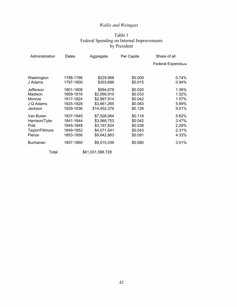
Wallis and Weingast

42

Table 1Federal Spending on Internal Improvements

by President

Administration Dates Aggregate Per Capita Share of all

Federal Expenditure

Washington 1788-1796 $229,968 $0.009 0.74%J Adams 1797-1800 $303,896 $0.015 0.94%

Jefferson 1801-1808 $994,678 $0.020 1.36%Madison 1809-1816 $2,066,910 $0.033 1.52%Monroe 1817-1824 $2,997,914 $0.042 1.57%J Q Adams 1825-1828 $3,861,265 $0.083 5.89%Jackson 1829-1836 $14,452,376 $0.129 9.51%

Van Buren 1837-1840 $7,528,064 $0.118 5.62%Harrison/Tyler 1841-1844 $3,068,753 $0.042 3.47%Polk 1845-1848 $3,197,824 $0.038 2.29%Taylor/Fillmore 1849-1852 $4,071,541 $0.043 2.31%Pierce 1853-1856 $9,642,863 $0.091 4.33%

Buchanan 1857-1860 $9,515,536 $0.080 3.51%

Total $61,931,588.728

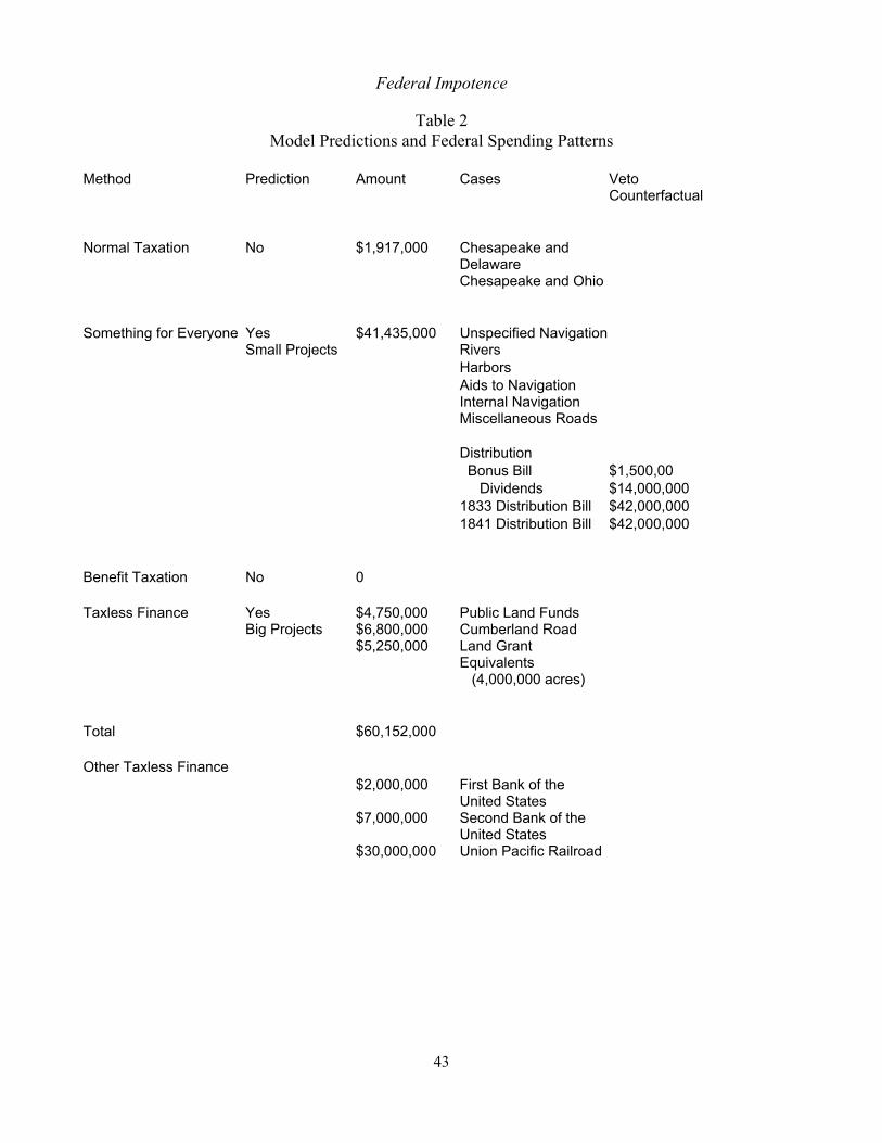
Federal Impotence

43

Table 2Model Predictions and Federal Spending Patterns

Method Prediction Amount Cases VetoCounterfactual

Normal Taxation No $1,917,000 Chesapeake andDelawareChesapeake and Ohio

Something for Everyone Yes $41,435,000 Unspecified NavigationSmall Projects Rivers

HarborsAids to NavigationInternal NavigationMiscellaneous Roads

Distribution Bonus Bill $1,500,00 Dividends $14,000,0001833 Distribution Bill $42,000,0001841 Distribution Bill $42,000,000

Benefit Taxation No 0

Taxless Finance Yes $4,750,000 Public Land FundsBig Projects $6,800,000 Cumberland Road

$5,250,000 Land GrantEquivalents (4,000,000 acres)

Total $60,152,000

Other Taxless Finance$2,000,000 First Bank of the

United States$7,000,000 Second Bank of the

United States$30,000,000 Union Pacific Railroad

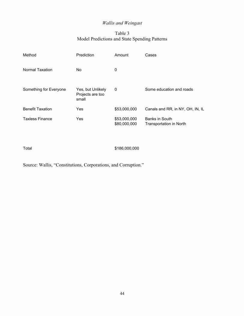
Wallis and Weingast

44

Table 3Model Predictions and State Spending Patterns

Method Prediction Amount Cases

Normal Taxation No 0

Something for Everyone Yes, but Unlikely 0 Some education and roadsProjects are too small

Benefit Taxation Yes $53,000,000 Canals and RR, in NY, OH, IN, IL

Taxless Finance Yes $53,000,000 Banks in South$80,000,000 Transportation in North

Total $186,000,000

Source: Wallis, “Constitutions, Corporations, and Corruption.”

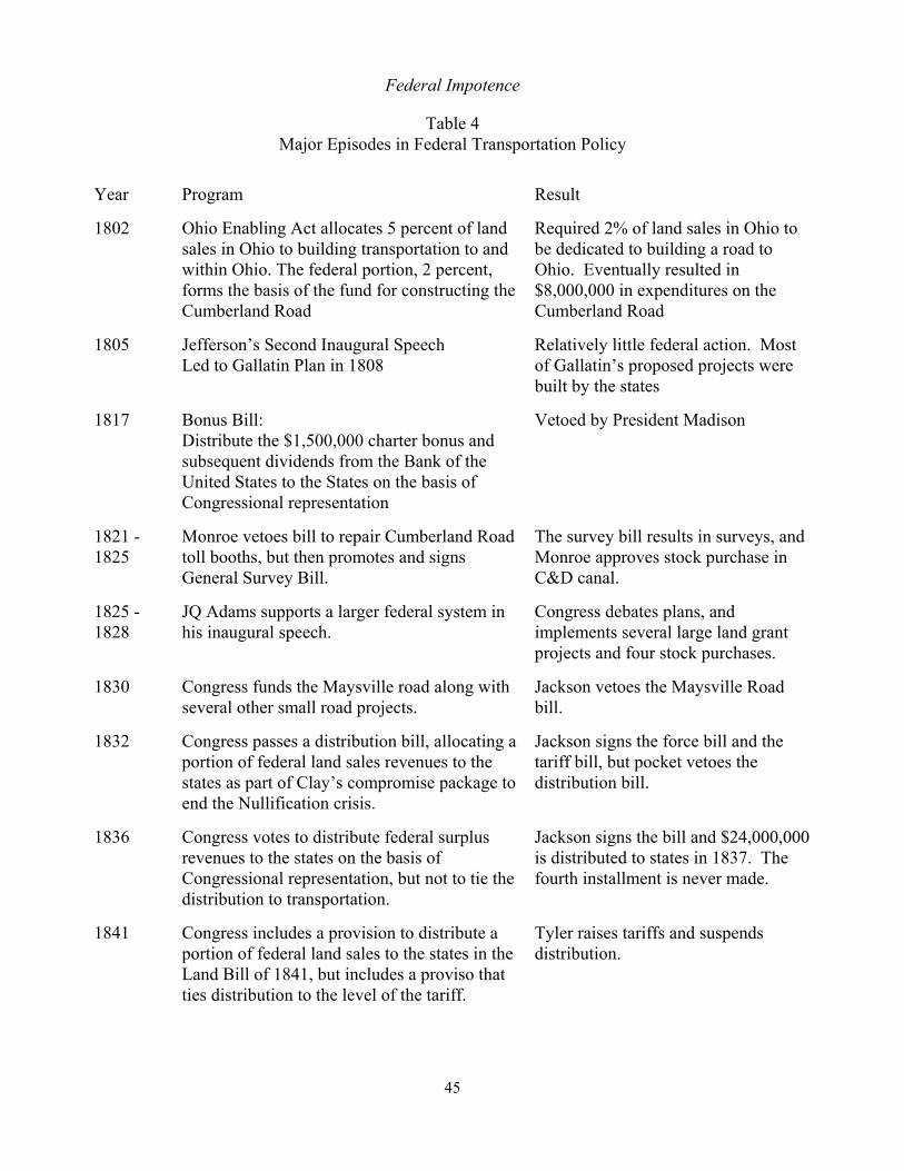
Federal Impotence

45

Table 4Major Episodes in Federal Transportation Policy

Year Program Result

1802 Ohio Enabling Act allocates 5 percent of landsales in Ohio to building transportation to andwithin Ohio. The federal portion, 2 percent,forms the basis of the fund for constructing theCumberland Road

Required 2% of land sales in Ohio tobe dedicated to building a road toOhio. Eventually resulted in$8,000,000 in expenditures on theCumberland Road

1805 Jefferson’s Second Inaugural SpeechLed to Gallatin Plan in 1808

Relatively little federal action. Mostof Gallatin’s proposed projects werebuilt by the states

1817 Bonus Bill:Distribute the $1,500,000 charter bonus andsubsequent dividends from the Bank of theUnited States to the States on the basis ofCongressional representation

Vetoed by President Madison

1821 - 1825

Monroe vetoes bill to repair Cumberland Roadtoll booths, but then promotes and signsGeneral Survey Bill.

The survey bill results in surveys, andMonroe approves stock purchase inC&D canal.

1825 -1828

JQ Adams supports a larger federal system inhis inaugural speech.

Congress debates plans, andimplements several large land grantprojects and four stock purchases.

1830 Congress funds the Maysville road along withseveral other small road projects.

Jackson vetoes the Maysville Roadbill.

1832 Congress passes a distribution bill, allocating aportion of federal land sales revenues to thestates as part of Clay’s compromise package toend the Nullification crisis.

Jackson signs the force bill and thetariff bill, but pocket vetoes thedistribution bill.

1836 Congress votes to distribute federal surplusrevenues to the states on the basis ofCongressional representation, but not to tie thedistribution to transportation.

Jackson signs the bill and $24,000,000is distributed to states in 1837. Thefourth installment is never made.

1841 Congress includes a provision to distribute aportion of federal land sales to the states in theLand Bill of 1841, but includes a proviso thatties distribution to the level of the tariff.

Tyler raises tariffs and suspendsdistribution.

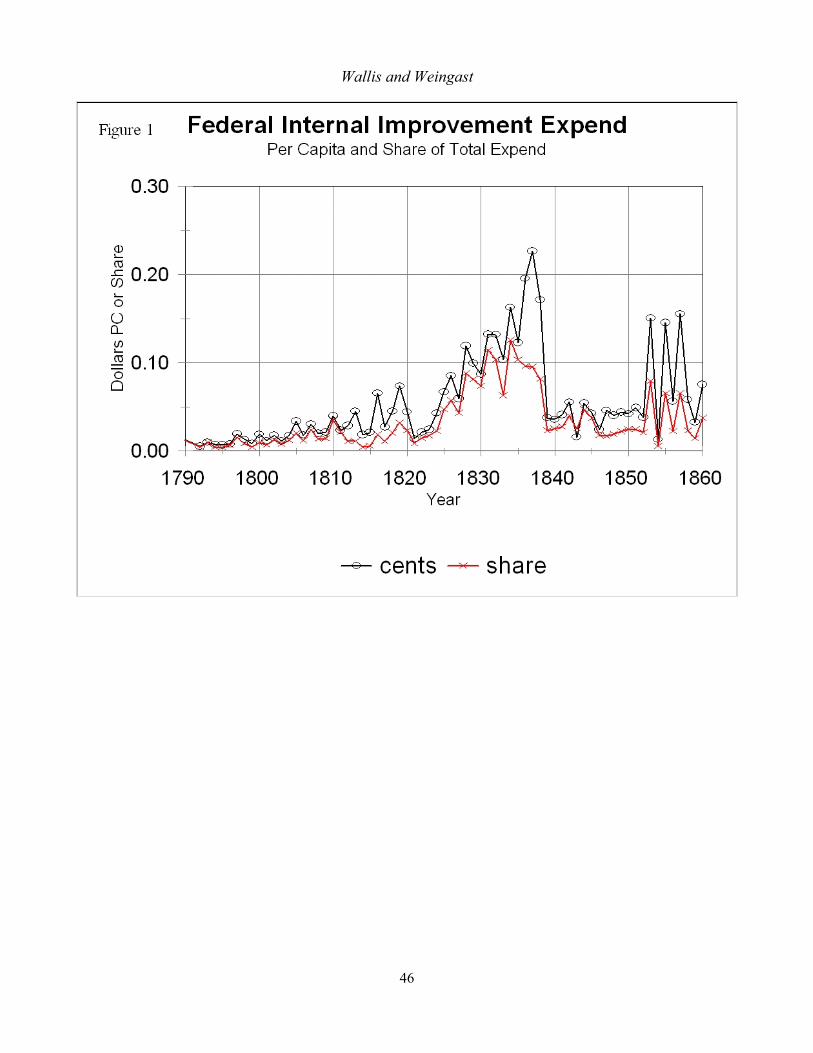
Wallis and Weingast

46

Documents

Equilibrium Federal Impotence