Embed Size (px)
Citation preview

Equilibrium

Market Equilibrium
A market is in equilibrium when total quantity demanded by buyers equals total quantity supplied by sellers.
An equilibrium situation is one where agents are choosing the best possible actions and the behaviors of all agents are mutually consistent.

Market Equilibrium It turns out that the equilibrium outcome
of a competitive market is Pareto efficient. At any amount of output less than the equilibrium level there is at least one producer willing to supply extra quantity of the good at a price that is less than the price at least one consumer is willing to pay. Therefore, we can improve the situation of at least two people without hurting anybody else.

Market EquilibriumThe equilibrium outcome of a
competitive market is the only Pareto efficient outcome.

Market Equilibrium
p
D(p)
q=D(p)
Marketdemand
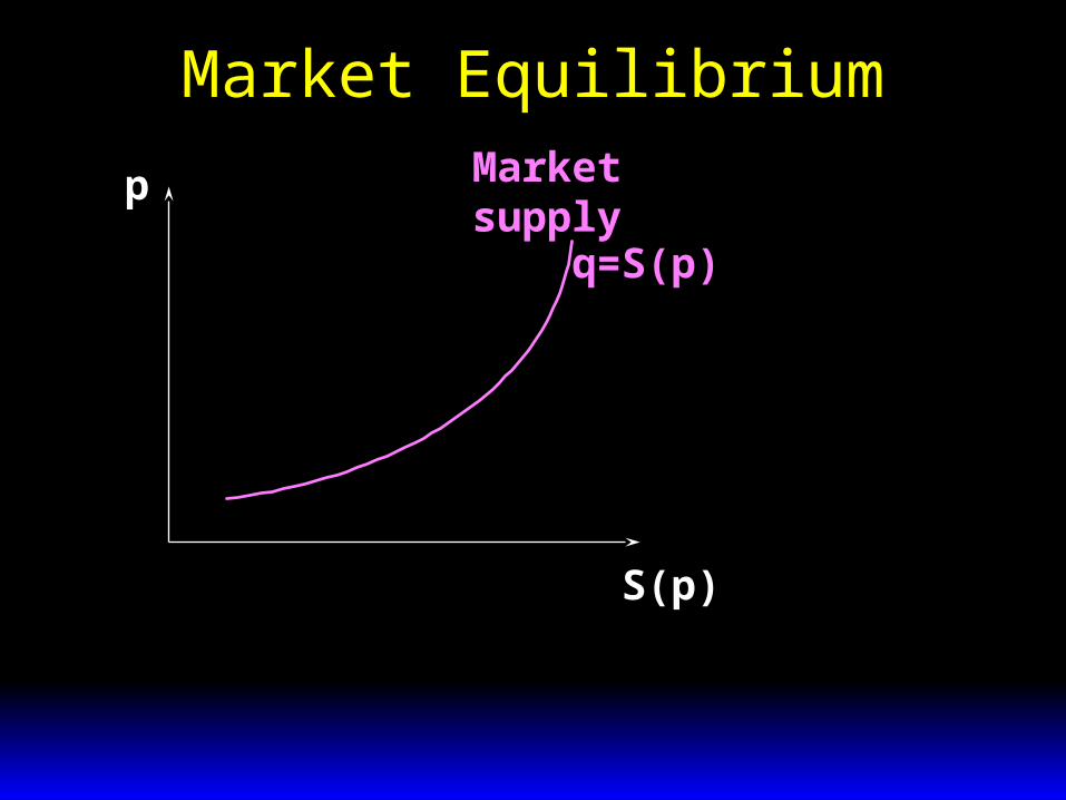
Market Equilibrium
p
S(p)
Marketsupply
q=S(p)

Market Equilibrium
p
D(p), S(p)
q=D(p)
Marketdemand
Marketsupply
q=S(p)

Market Equilibrium
p
D(p), S(p)
q=D(p)
Marketdemand
Marketsupply
q=S(p)
p*
q*
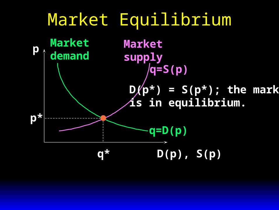
Market Equilibrium
p
D(p), S(p)
q=D(p)
Marketdemand
Marketsupply
q=S(p)
p*
q*
D(p*) = S(p*); the marketis in equilibrium.

Market Equilibrium
p
D(p), S(p)
q=D(p)
Marketdemand
Marketsupply
q=S(p)
p*
S(p’)
D(p’) < S(p’); an excessof quantity supplied overquantity demanded.
p’
D(p’)

Market Equilibrium
p
D(p), S(p)
q=D(p)
Marketdemand
Marketsupply
q=S(p)
p*
S(p’)
D(p’) < S(p’); an excessof quantity supplied overquantity demanded.
p’
D(p’)
Market price must fall towards p*.

Market Equilibrium
p
D(p), S(p)
q=D(p)
Marketdemand
Marketsupply
q=S(p)
p*
D(p”)
D(p”) > S(p”); an excessof quantity demandedover quantity supplied.
p”
S(p”)
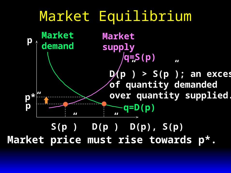
Market Equilibrium
p
D(p), S(p)
q=D(p)
Marketdemand
Marketsupply
q=S(p)
p*
D(p”)
D(p”) > S(p”); an excessof quantity demandedover quantity supplied.
p”
S(p”)
Market price must rise towards p*.

Market Equilibrium
The effects of setting a maximum price
The effects of setting a minimum price

Market EquilibriumDemand shifts and motives:
- income,- preferences,- prices of substitutes or complements
have changed,- expectations of future changes in
income or prices,- population,- taxes on consumption

Market EquilibriumSupply shifts and motives:
- production technology,- changes in the prices of
production factors (wages, prices of raw materials, interest rate, …),
- number of producers,- expectations of future price
changes,- taxes on production

Market Equilibrium The effects of elasticities on price and
quantity variations: when one curve is very inelastic, price accommodates; when one curve is very elastic, quantity accommodates
(“One of DeBeers’ main roles is to maintain the notion that diamonds are a scarce commodity. This they do by means of advertising and by purchasing excess supplies when that is needed to avoid price decreases: as a matter of principle, prices are never lowered by DeBeers.”)

Market Equilibrium
An example of calculating a market equilibrium when the market demand and supply curves are linear.
D p a bp( ) S p c dp( )

Market Equilibrium
p
D(p), S(p)
D(p) = a-bp
Marketdemand
Marketsupply
S(p) = c+dp
p*
q*
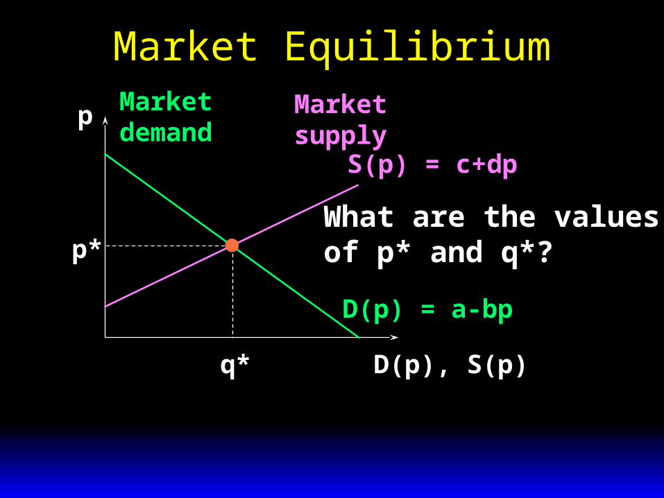
Market Equilibrium
p
D(p), S(p)
D(p) = a-bp
Marketdemand
Marketsupply
S(p) = c+dp
p*
q*
What are the valuesof p* and q*?

Market EquilibriumD p a bp( ) S p c dp( )
At the equilibrium price p*, D(p*) = S(p*).
Market EquilibriumD p a bp( ) S p c dp( )
At the equilibrium price p*, D(p*) = S(p*).That is, a bp c dp * *

Market EquilibriumD p a bp( ) S p c dp( )
At the equilibrium price p*, D(p*) = S(p*).That is, a bp c dp * *
which gives pa cb d
*
Market EquilibriumD p a bp( ) S p c dp( )
At the equilibrium price p*, D(p*) = S(p*).That is, a bp c dp * *
which gives pa cb d
*
and q D p S pad bcb d
* * *( ) ( ) .

Market Equilibrium
p
D(p), S(p)
D(p) = a-bp
Marketdemand
Marketsupply
S(p) = c+dpp
a cb d
*
dbbcad
q*

Market Equilibrium
Can we calculate the market equilibrium using the inverse market demand and supply curves?
Yes, it is the same calculation.

Market Equilibrium
Two special cases:quantity supplied is fixed,
independent of the market price, and
quantity supplied is extremely sensitive to the market price.

Market Equilibrium
p
q
D-1(q) = (a-q)/b
Marketdemand
q* = c
p* = D-1(q*); that is,p* = (a-c)/b.
p* =(a-c)/b
Market quantity supplied isfixed, independent of price.

Market EquilibriumMarket quantity supplied isextremely sensitive to price.
S-1(q) = p*.
p
q
p*
D-1(q) = (a-q)/b
Marketdemand
q* =a-bp*
p* = D-1(q*) = (a-q*)/b soq* = a-bp*
Quantity Taxes
A quantity tax levied at a rate of €t is a tax of €t paid on each unit traded.
If the tax is levied on sellers then it is an excise tax.
If the tax is levied on buyers then it is a sales tax.

Quantity Taxes
What is the effect of a quantity tax on a market’s equilibrium?
How are prices affected?How is the quantity traded affected?Who pays the tax?How are gains-to-trade altered?

Quantity Taxes
A tax rate t makes the price paid by buyers, pb, higher by t from the price received by sellers, ps.
p p tb s

Quantity Taxes
Even with a tax the market must clear.
I.e. quantity demanded by buyers at price pb must equal quantity supplied by sellers at price ps.
D p S pb s( ) ( )

Quantity Taxes
p p tb s D p S pb s( ) ( )and
describe the market’s equilibrium.Notice that these conditions apply nomatter if the tax is levied on sellers or onbuyers.

Quantity Taxes
p p tb s D p S pb s( ) ( )and
describe the market’s equilibrium.Notice that these two conditions apply nomatter if the tax is levied on sellers or onbuyers.
Hence, a tax rate €t has thesame effect no matter the side of themarket on which it is levied.

Quantity Taxes & Market Equilibrium
p
D(p), S(p)
Marketdemand
Marketsupply
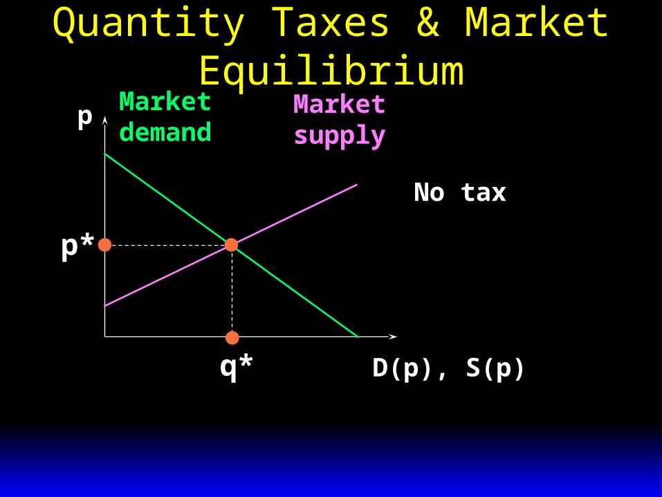
p*
q*
No tax

Quantity Taxes & Market Equilibrium
p
D(p), S(p)
Marketdemand
Marketsupply
p*
q*
€t
An excise taxraises the marketsupply curve by €t

Quantity Taxes & Market Equilibrium
p
D(p), S(p)
Marketdemand
Marketsupply
p*
q*
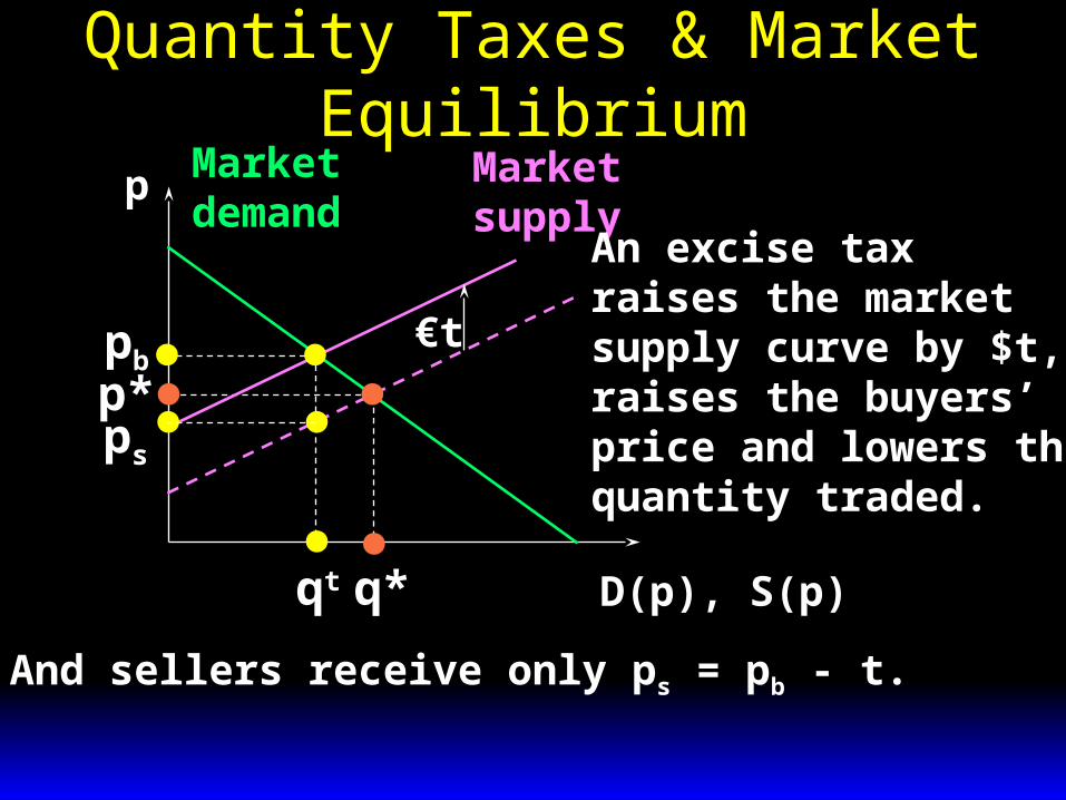
An excise taxraises the marketsupply curve by €t,raises the buyers’price and lowers thequantity traded.
€tpb
qt
Quantity Taxes & Market Equilibrium
p
D(p), S(p)
Marketdemand
Marketsupply
p*
q*
An excise taxraises the marketsupply curve by $t,raises the buyers’price and lowers thequantity traded.
€tpb
qt
And sellers receive only ps = pb - t.
ps
Quantity Taxes & Market Equilibrium
p
D(p), S(p)
Marketdemand
Marketsupply
p*
q*
No tax

Quantity Taxes & Market Equilibrium
p
D(p), S(p)
Marketdemand
Marketsupply
p*
q*
A sales tax lowersthe market demandcurve by €t
€t

Quantity Taxes & Market Equilibrium
p
D(p), S(p)
Marketdemand
Marketsupply
p*
q*
An sales tax lowersthe market demandcurve by €t, lowersthe sellers’ price andreduces the quantitytraded.€t
qt
ps

Quantity Taxes & Market Equilibrium
p
D(p), S(p)
Marketdemand
Marketsupply
p*
q*
An sales tax lowersthe market demandcurve by €t, lowersthe sellers’ price andreduces the quantitytraded.€t
pbpb
qt
pb
And buyers pay pb = ps + t.
ps
Quantity Taxes & Market Equilibrium
p
D(p), S(p)
Marketdemand
Marketsupply
p*
q*
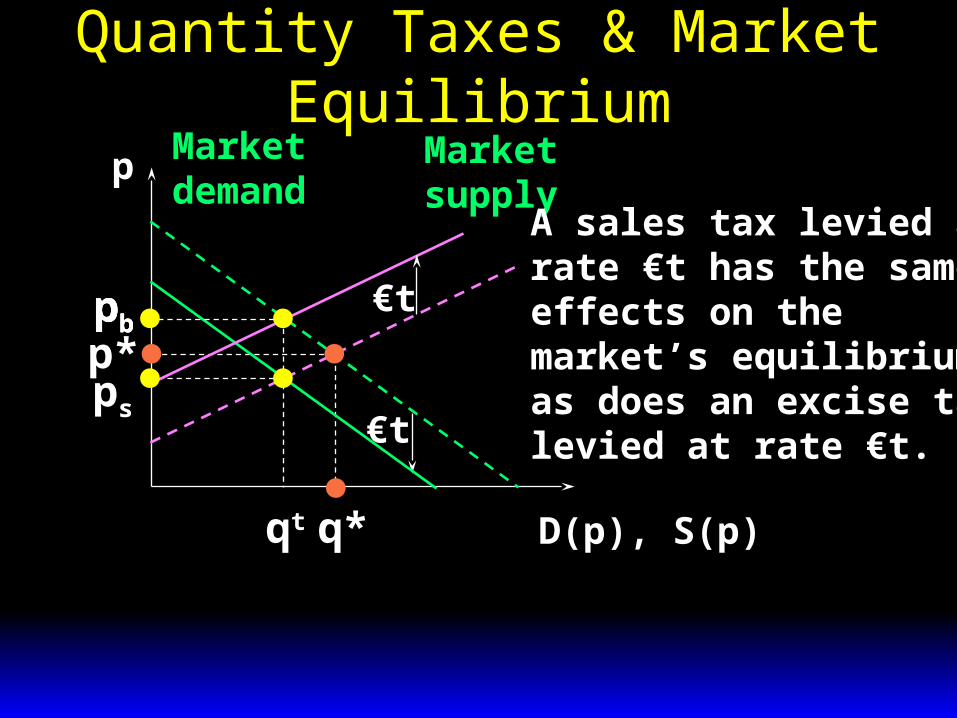
A sales tax levied atrate €t has the sameeffects on themarket’s equilibriumas does an excise taxlevied at rate €t.€t
pbpb
qt
pb
ps
€t

Quantity Taxes & Market Equilibrium
Who pays the tax of €t per unit traded?
The division of the €t between buyers and sellers is the economic incidence of the tax.

Quantity Taxes & Market Equilibrium
p
D(p), S(p)
Marketdemand
Marketsupply
p*
q*
pbpb
qt
pb
ps
Quantity Taxes & Market Equilibrium
p
D(p), S(p)
Marketdemand
Marketsupply
p*
q*
pbpb
qt
pb
ps
Tax paid by buyers
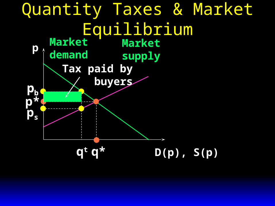
Quantity Taxes & Market Equilibrium
p
D(p), S(p)
Marketdemand
Marketsupply
p*
q*
pbpb
qt
pb
psTax paid by sellers

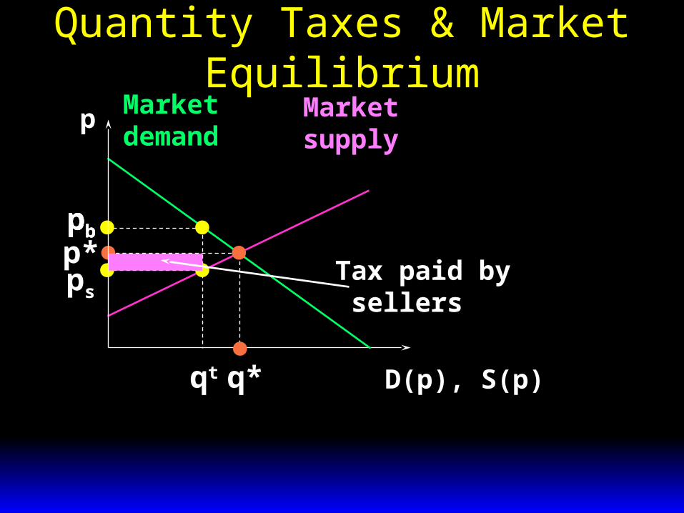
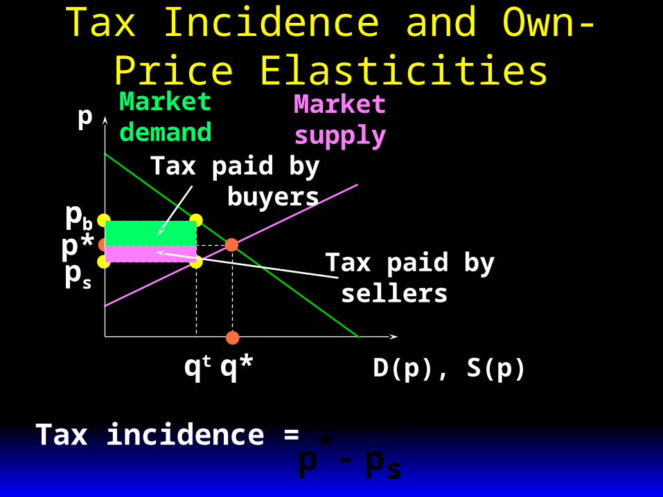
Quantity Taxes & Market Equilibrium
p
D(p), S(p)
Marketdemand
Marketsupply
p*
q*
pbpb
qt
pb
ps
Tax paid by buyers
Tax paid by sellers
Quantity Taxes & Market Equilibrium
E.g. suppose the market demand and supply curves are linear.
D p a bpb b( ) S p c dps s( )

Quantity Taxes & Market Equilibrium
andD p a bpb b( ) S p c dps s( ) .
Quantity Taxes & Market Equilibrium
and
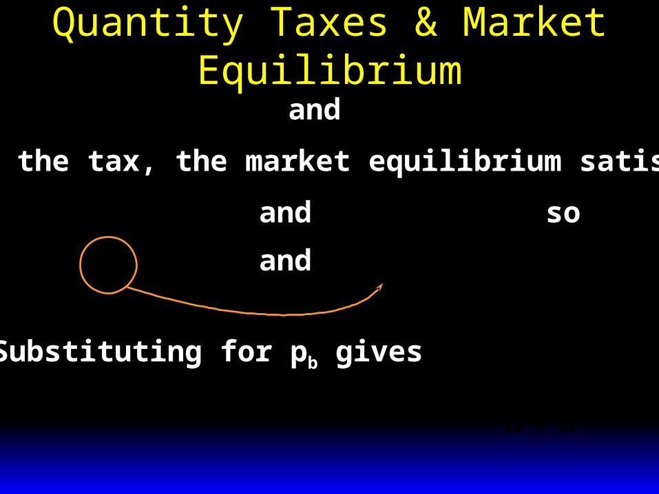
With the tax, the market equilibrium satisfies
and so
and
D p a bpb b( ) S p c dps s( ) .
p p tb s D p S pb s( ) ( )
p p tb s a bp c dpb s .
Quantity Taxes & Market Equilibrium
D p a bpb b( ) S p c dps s( ) . and
With the tax, the market equilibrium satisfies
p p tb s D p S pb s( ) ( )and so
p p tb s a bp c dpb s .and
Substituting for pb gives
a b p t c dp pa c bt
b ds s s
( ) .

Quantity Taxes & Market Equilibrium
pa c bt
b ds and p p tb s give
The quantity traded at equilibrium is
q D p S p
a bpad bc bdt
b d
tb s
b
( ) ( )
.
pa c dt
b db

Quantity Taxes & Market Equilibrium
pa c bt
b ds
pa c dt
b db
qad bc bdt
b dt
As t 0, ps and pb theequilibrium price ifthere is no tax (t = 0) and qt the quantity traded at equilibriumwhen there is no tax.
ad bcb d
,
*,pdbca

Quantity Taxes & Market Equilibrium
pa c bt
b ds
pa c dt
b db
qad bc bdt
b dt
As t increases, ps falls,
pb rises,
and qt falls.

Quantity Taxes & Market Equilibrium
pa c bt
b ds
pa c dt
b db
qad bc bdt
b dt
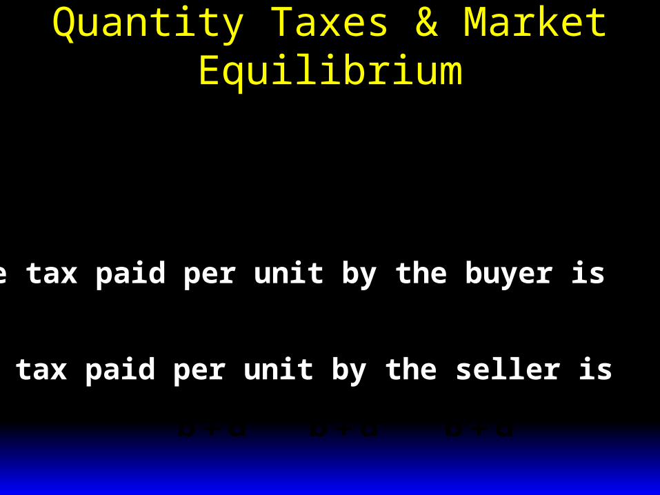
The tax paid per unit by the buyer isp p
a c dtb d
a cb d
dtb db
* .
Quantity Taxes & Market Equilibrium
pa c bt
b ds
pa c dt
b db
qad bc bdt
b dt
The tax paid per unit by the buyer isp p
a c dtb d
a cb d
dtb db
* .
The tax paid per unit by the seller isp p
a cb d
a c btb d
btb ds
* .

Quantity Taxes & Market Equilibrium
pa c bt
b ds
pa c dt
b db
qad bc bdt
b dt
The total tax paid (by buyers and sellerscombined) is
T tq tad bc bdt
b dt
.
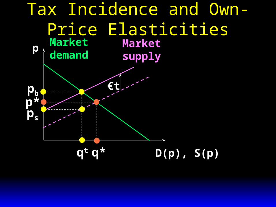
Tax Incidence and Own-Price Elasticities
The incidence of a quantity tax depends upon the own-price elasticities of demand and supply.
Tax Incidence and Own-Price Elasticities
p
D(p), S(p)
Marketdemand
Marketsupply
p*
q*
€tpb
qt
ps
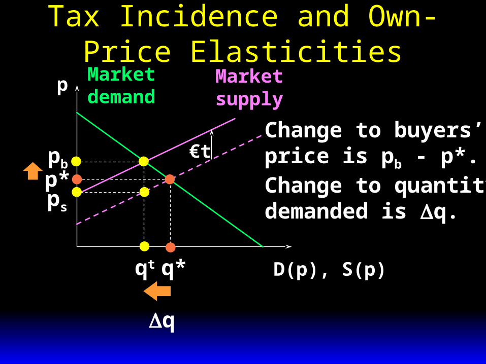
Tax Incidence and Own-Price Elasticities
p
D(p), S(p)
Marketdemand
Marketsupply
p*
q*
€tpb
qt
ps
Change to buyers’price is pb - p*.Change to quantitydemanded is q.
q
Tax Incidence and Own-Price Elasticities
Around p = p* the own-price elasticityof demand is approximately
*
*
*
ppp
bD

Tax Incidence and Own-Price Elasticities
Around p = p* the own-price elasticityof demand is approximately
*
**
*
*
*
q
pqpp
ppp
Db
bD

Tax Incidence and Own-Price Elasticities
p
D(p), S(p)
Marketdemand
Marketsupply
p*
q*
€tpb
qt
ps
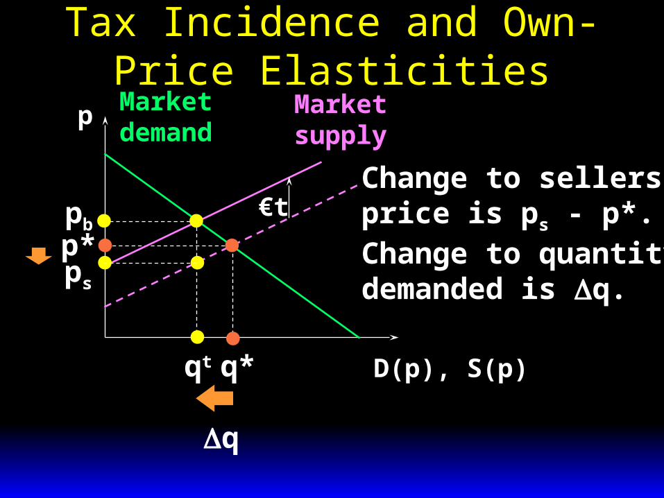
Tax Incidence and Own-Price Elasticities
p
D(p), S(p)
Marketdemand
Marketsupply
p*
q*
€tpb
qt
ps
Change to sellers’price is ps - p*.Change to quantitydemanded is q.
q
Tax Incidence and Own-Price Elasticities
Around p = p* the own-price elasticityof supply is approximately
Ss
q
q
p p
p
*
*
*

Tax Incidence and Own-Price Elasticities
Around p = p* the own-price elasticityof supply is approximately
Ss
sS
q
q
p p
p
p pq p
q
*
*
*
**
*.

Tax Incidence and Own-Price Elasticities
p
D(p), S(p)
Marketdemand
Marketsupply
p*
q*
pbpb
qt
pb
ps
Tax paid by buyers
Tax paid by sellers
Tax Incidence and Own-Price Elasticities
p
D(p), S(p)
Marketdemand
Marketsupply
p*
q*
pbpb
qt
pb
ps
Tax paid by buyers
Tax paid by sellers
Tax incidence = p p
p pb
s
*
*.

Tax Incidence and Own-Price Elasticities
Tax incidence = p p
p pb
s
*
*.
.*
**
q
pqpp
Db
p p
q p
qs
S
*
*
*.

Tax Incidence and Own-Price Elasticities
Tax incidence = p p
p pb
s
*
*.
.*
*
*
q
pqpp
Db
p p
q p
qs
S
*
*
*.
So
D
S
s
b
pp
pp
*
*
Tax Incidence and Own-Price Elasticities
Tax incidence is
The fraction of a €t quantity tax paidby buyers rises as supply becomes moreown-price elastic or as demand becomesless own-price elastic.
D
S
s
b
pp
pp
*
*
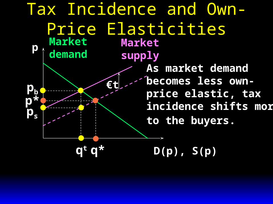
Tax Incidence and Own-Price Elasticities
p
D(p), S(p)
Marketdemand
Marketsupply
p*
q*
€tpb
qt
ps
As market demandbecomes less own-price elastic, taxincidence shifts moreto the buyers.

Tax Incidence and Own-Price Elasticities
p
D(p), S(p)
Marketdemand
Marketsupply
p*
q*
€tpb
qt
ps
As market demandbecomes less own-price elastic, taxincidence shifts moreto the buyers.

Tax Incidence and Own-Price Elasticities
p
D(p), S(p)
Marketdemand
Marketsupply
ps= p*
€tpb
qt = q*
As market demandbecomes less own-price elastic, taxincidence shifts moreto the buyers.
When D = 0, buyers pay the entire tax, even though it is levied on the sellers.

Tax Incidence and Own-Price Elasticities
Similarly, the fraction of a €t quantitytax paid by sellers rises as supplybecomes less own-price elastic or asdemand becomes more own-price elastic.

Deadweight Loss and Own-Price Elasticities
A quantity tax imposed on a competitive market reduces the quantity traded and so reduces gains-to-trade (i.e. the sum of Consumers’ and Producers’ Surpluses).
The lost total surplus is the tax’s deadweight loss, or excess burden.

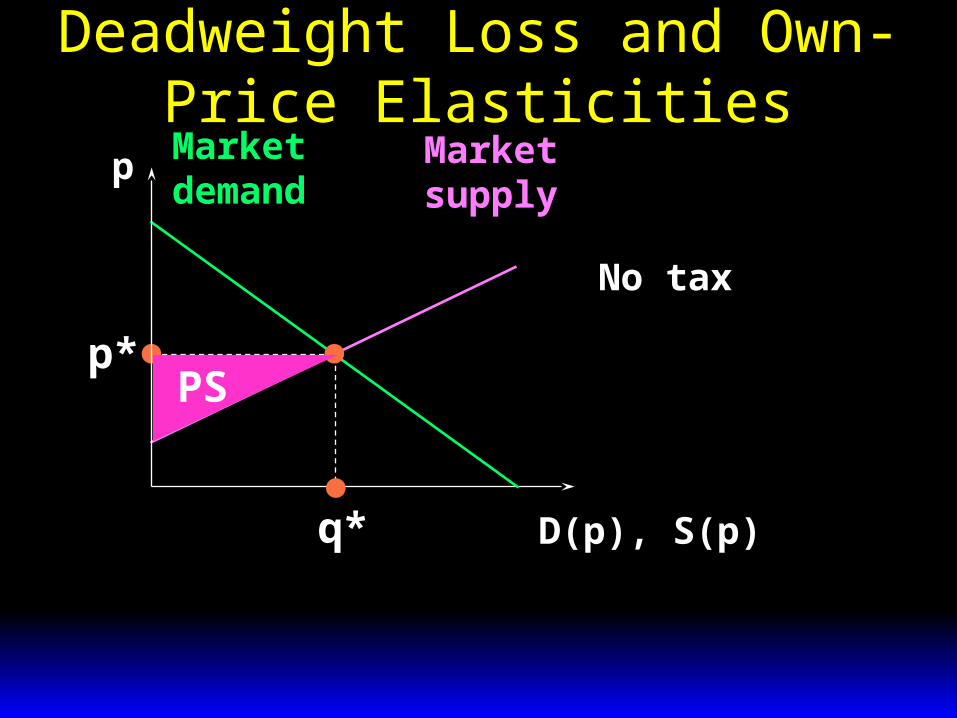
Deadweight Loss and Own-Price Elasticities
p
D(p), S(p)
Marketdemand
Marketsupply
p*
q*
No tax
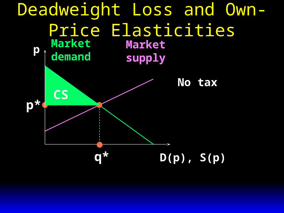
Deadweight Loss and Own-Price Elasticities
p
D(p), S(p)
Marketdemand
Marketsupply
p*
q*
No taxCS
Deadweight Loss and Own-Price Elasticities
p
D(p), S(p)
Marketdemand
Marketsupply
p*
q*
No tax
PS

Deadweight Loss and Own-Price Elasticities
p
D(p), S(p)
Marketdemand
Marketsupply
p*
q*
No taxCS
PS

Deadweight Loss and Own-Price Elasticities
p
D(p), S(p)
Marketdemand
Marketsupply
p*
q*
No taxCS
PS

Deadweight Loss and Own-Price Elasticities
p
D(p), S(p)
Marketdemand
Marketsupply
p*
q*
€tpb
qt
ps
CS
PS
The tax reducesboth CS and PS

Deadweight Loss and Own-Price Elasticities
p
D(p), S(p)
Marketdemand
Marketsupply
p*
q*
€tpb
qt
ps
CS
PS
The tax reducesboth CS and PS,transfers surplusto government
Tax

Deadweight Loss and Own-Price Elasticities
p
D(p), S(p)
Marketdemand
Marketsupply
p*
q*
€tpb
qt
ps
CS
PS
The tax reducesboth CS and PS,transfers surplusto government
Tax

Deadweight Loss and Own-Price Elasticities
p
D(p), S(p)
Marketdemand
Marketsupply
p*
q*
€tpb
qt
ps
CS
PS
The tax reducesboth CS and PS,transfers surplusto government,and lowers total surplus.
Tax
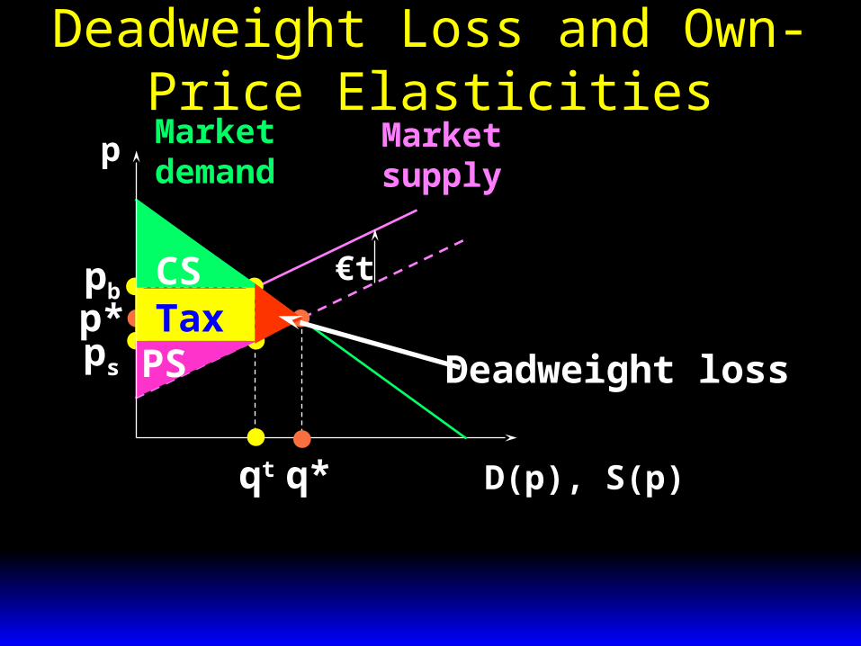
Deadweight Loss and Own-Price Elasticities
p
D(p), S(p)
Marketdemand
Marketsupply
p*
q*
€tpb
qt
ps
CS
PSTax
Deadweight loss

Deadweight Loss and Own-Price Elasticities
p
D(p), S(p)
Marketdemand
Marketsupply
p*
q*
€tpb
qt
ps Deadweight loss

Deadweight Loss and Own-Price Elasticities
p
D(p), S(p)
Marketdemand
Marketsupply
p*
q*
€tpb
qt
ps
Deadweight loss fallsas market demandbecomes less own-price elastic.

Deadweight Loss and Own-Price Elasticities
p
D(p), S(p)
Marketdemand
Marketsupply
p*
q*
€tpb
qt
ps
Deadweight loss fallsas market demandbecomes less own-price elastic.

Deadweight Loss and Own-Price Elasticities
p
D(p), S(p)
Marketdemand
Marketsupply
ps= p*
€tpb
qt = q*
Deadweight loss fallsas market demandbecomes less own-price elastic.
When D = 0, the tax causes no deadweight loss.

Deadweight Loss and Own-Price Elasticities
Deadweight loss due to a quantity tax rises as either market demand or market supply becomes more own-price elastic.
If either D = 0 or S = 0 then the deadweight loss is zero.

Fiscal Revenue
Fiscal revenue decreases for t sufficiently large, because market transactions are highly reduced: the Laffer curve.
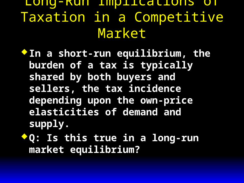
Long-Run Implications of Taxation in a Competitive Market
In a short-run equilibrium, the burden of a tax is typically shared by both buyers and sellers, the tax incidence depending upon the own-price elasticities of demand and supply.
Q: Is this true in a long-run market equilibrium?

Long-Run Implications of Taxation in a Competitive Market
LR supply (no tax)
p
X,Y
Market demand
Qe
pe

Long-Run Implications of Taxation in a Competitive Market
LR supply (no tax)
p
X,Y
Market demand
Qe
ps=pe
LR supply (with tax)
Qt
pb = pe+t
t

Long-Run Implications of Taxation in a Competitive Market
LR supply (no tax)
p
X,Y
Market demand
Qe
ps=pe
LR supply (with tax)
Qt
pb = pe+t
t
In the long-run thebuyers pay all of asales or an excise tax.