Equilibrium Prices in the Presence of

Delegated Portfolio Management∗

Domenico CuocoThe Wharton School

University of PennsylvaniaPhiladelphia, PA 19104

Tel: (215) 898-8290cuoco@wharton.upenn.edu

Ron Kaniel†

Fuqua School of BusinessDuke University

Durham, NC 27708Tel: (919) 660-7656ron.kaniel@duke.edu

This revision: November 2007

Abstract

This paper analyzes the asset pricing implications of commonly-used portfolio manage-ment contracts linking the compensation of fund managers to the excess return of themanaged portfolio over a benchmark portfolio. The contract parameters, the extent ofdelegation and equilibrium prices are all determined endogenously within the model weconsider. Symmetric (“fulcrum”) performance fees distort the allocation of managedportfolios in a way that induces a significant and unambiguous positive effect on theprices of the assets included in the benchmark and a negative effect on the Sharperatios. Asymmetric performance fees have more complex effects on equilibrium pricesand Sharpe ratios, with the signs of these effects fluctuating stochastically over time inresponse to variations in the funds’ excess performance.

∗An earlier version of this paper was circulated with the title “General Equilibrium Implications ofFund Managers’ Compensation Fees”. We would like to thank Phil Dybvig and Pete Kyle for very helpfulcomments. The paper has also benefited from discussions with Andy Abel, Simon Gervais, Bruce Grundy,Rich Kihlstrom, Jose Marin and seminar participants at the University of Brescia, University of BritishColumbia, Carnegie Mellon, University of Chicago, Cornell, Duke, HEC, INSEAD, London Business School,University of North Carolina, Northwestern, Rochester, University of Salerno, University of Texas at Austin,University of Utah, Washington University, Wharton, the 1999 “Accounting and Finance in Tel-Aviv”conference and the 2001 AFA meeting.†Corresponding author.

1 Introduction

In modern economies, a significant share of financial wealth is delegated to professionalportfolio managers rather than managed directly by the owners, creating an agency rela-tionship. In the U.S., as of 2004, mutual funds managed assets in excess of $8 trillion, hedgefunds managed about $1 trillion and pension funds more than $12 trillion. In other indus-trialized countries, the percentage of financial assets managed through portfolio managersis even larger than in the U.S. (see, e.g., Bank for International Settlements (2003)).

While the theoretical literature on optimal compensation of portfolio managers in dy-namic settings points to contracts that are likely to have very complicated path depen-dencies,1 the industry practice seems to favor relatively simple compensation schemes thattypically include a component that depends linearly on the value of the managed assetsplus a component that is linearly or non-linearly related to the excess performance of themanaged portfolio over a benchmark.

In 1970, the U.S. Congress amended the Investment Advisers Act of 1940 so as to allowcontracts with registered investment companies to include performance-based compensa-tion, provided that this compensation is of the “fulcrum” type, that is, provided that itincludes penalties for underperforming the chosen benchmark that are symmetric to thebonuses for exceeding it. In 1985, the SEC approved the use of performance-based fees incontracts in which the client has either at least $500,000 under management or a net worthof at least $1 million. Performance-based fees were also approved by the Department ofLabor in August 1986 for ERISA-governed pension funds. As of 2004, 50% of U.S. cor-porate pension funds with assets above $5 billion, 35% of all U.S. pension funds and 9%of all U.S. mutual funds used performance-based fees.2 Furthermore, Brown, Harlow andStarks (1996), Chevalier and Ellison (1997) and Sirri and Tufano (1998) have documentedthat, even when mutual fund managers do not receive explicit incentive fees, an implicitnonlinear performance-based compensation still arises with periodic proportional fees as aresult of the fact that the net investment flow into mutual funds varies in a convex fashionas a function of recent performance.3

Given the size of the portfolio management industry, studying the implications of thisdelegation and of the fee structures commonly used in the industry on equilibrium assetprices appears to be a critical task. The importance of models addressing the implicationsof agency for asset pricing was emphasized by Allen (2001): “In the standard asset-pricing

1A distinctive feature of the agency problem arising from portfolio management is that the agent’sactions (the investment strategy and possibly the effort spent acquiring information about securities’ returns)affect both the drift and the volatility of the relevant state variable (the value of the managed portfolio),although realistically the drift and the volatility cannot be chosen independently. This makes the problemsignificantly more complex than the one considered in the classic paper by Holstrom and Milgrom (1987) andits extensions. With a couple of exceptions, as noted by Stracca (2006) in his recent survey of the literatureon delegated portfolio managent, “the literature has reached more negative rather than constructive results,and the search for an optimal contract has proved to be inconclusive even in the most simple settings.”

2The use is concentrated in larger funds: the percentages of assets under management controlled bymutual funds charging performance fees out of funds managing assets of $0.25-1 billion, $1-5 billion, $5-10billion, and above $10 billion were 2.8%, 4.4%, 9.2%, and 14.2% respectively (data obtained from GreenwichAssociates and the Investment Company Institute).

3Lynch and Musto (2003) and Berk and Green (2004) provide models in which this convex relationshipbetween flows and performance arises endogenously.

1

paradigm it is assumed investors directly invest their wealth in markets. While this was anappropriate assumption for the U.S. in the 1950 when individuals directly held over 90% ofcorporate equities, or even in 1970 when the figure was 68%, it has become increasingly lessappropriate as time has progressed [. . .] For actively managed funds, the people that makethe ultimate investment decisions are not the owners. If the people making the investmentdecisions obtain a high reward when things go well and a limited penalty if they go badlythey will be willing to pay more than the discounted cash flow for an asset. This is the typeof incentive scheme that many financial institutions give to investment managers.”

Existing theoretical research on delegated portfolio management has been primarilyrestricted to partial equilibrium settings and has focused on two main areas. The first ex-amines the agency problem that arises between investors and portfolio managers, studyinghow compensation contracts should be structured: it includes Bhattacharya and Pflei-derer (1985), Starks (1987), Kihlstrom (1988), Stoughton (1993), Heinkel and Stoughton(1994), Admati and Pfleiderer (1997), Das and Sundaram (2002), Palomino and Prat (2003),Ou-Yang (2003), Larsen (2005), Liu (2005), Dybvig, Farnsworth and Carpenter (2006),Cadenillas, Cvitanic and Zapatero (2007) and Cvitanic, Wan and Zhang (2007). The sec-ond examines how commonly-observed incentive contracts impact managers’ decisions: itincludes Grinblatt and Titman (1989), Roll (1992), Carpenter (2000), Chen and Pennac-chi (2005), Hugonnier and Kaniel (2006) and Basak, Pavlova and Shapiro (2007).

We complement this literature by considering a different problem. As in the literatureon optimal behavior of portfolio managers, we take the parametric class of contracts asexogenously given, motivated by commonly observed fee structures. However, we carry theanalysis beyond partial equilibrium by studying how the behavior of portfolio managersaffects equilibrium prices when the extent of portfolio delegation and the parameters of themanagement contract are all determined endogenously.

A first step in studying the implications of delegated portfolio management on assetreturns was made by Brennan (1993), who considered a static mean-variance economy withtwo types of investors: individual investors (assumed to be standard mean-variance opti-mizers) and “agency investors” (assumed to be concerned with the mean and the varianceof the difference between the return on their portfolio and the return on a benchmarkportfolio). Equilibrium expected returns were shown to be characterized by a two-factormodel, with the two factors being the market and the benchmark portfolio. Closely-relatedmean-variance models have appeared in Gomez and Zapatero (2003) and Cornell and Roll(2005).4

To our knowledge, the only general equilibrium analyses of portfolio delegation in dy-namic settings are in two recent papers by Kapur and Timmermann (2005) and Arora, Juand Ou-Yang (2006). Kapur and Timmermann consider a restricted version of our modelwith mean-variance preferences, normal returns and fulcrum performance fees, while Arora,Ju and Ou-Yang assume CARA utilities and normal dividends and do not endogenize theextent of portfolio delegation: as a result of these assumptions, fulcrum performance feesare optimal in their model.5 More importantly, both papers consider settings with a single

4Brennan (1993) found mixed empirical support for the two-factor model over the period 1931–1991,while Gomez and Zapatero (2003) found stronger support over the period 1983–1997.

5In the model of Kapur and Timmerann, performance fees do not dominate fees depending only on theterminal value of the assets under managent.

2

risky asset. A key shortcoming of models with a single risky asset (or of static models) isthat they are unable to capture the shifting risk incentives of portfolio managers receivingimplicit or explicit performance fees (and hence the impact of these incentives on port-folio choices and equilibrium prices), as extensively described in both the theoretical andempirical literature.6

In contrast to the papers mentioned above, we study the asset pricing implications ofdelegated portfolio management in the context of a dynamic (continuous-time) model withmultiple risky assets and endogenous portfolio delegation. Specifically, we consider an econ-omy with a continuum of three types of agents: “active investors”, “fund investors” and“fund managers”. Active investors, who trade on their own account, choose a dynamic trad-ing strategy so as to maximize the expected utility of the terminal value of their portfolio.Fund investors, who implicitly face higher trading or information costs, invest in equitiesonly through mutual funds: therefore, their investment choices are limited to how much todelegate to fund managers, with the rest of their portfolio being invested in riskless assets.Fund managers, who are assumed not to have any private wealth, select a dynamic tradingstrategy so as to maximize the expected utility of their compensation.

The compensation contracts we consider are restricted to a parametric structure thatreplicates the contracts typically observed in practice, consisting of a combination of thefollowing components: a flat fee, a proportional fee depending on the total value of theassets under management, and a performance fee depending in a piecewise-linear manneron the differential between the return of the managed portfolio and that of a benchmarkportfolio.7

Departing from the traditional formulation of principal-agent problems, we assume thatindividual fund investors are unable to make “take it or leave it” contract offers to fundmanagers and thus to extract the entire surplus from the agency relation: instead, we assumethat the market for fund investors is competitive, so that individual investors take the feestructure as given when deciding what fraction of their wealth to delegate.8 Similarly, weassume competition on the market for portfolio managers. The contract parameters areselected in our model so that they are constrained Pareto efficient, i.e., so that there isno other contract within our parametric class that provides both fund investors and fundmanagers with higher welfares.

As shown in Section 5, even when fund investors and fund managers have identical pref-erences, the principle of preference similarity (Ross (1973)) does not apply in our settingand asymmetric performance contracts Pareto-dominate purely proportional contracts (aswell as fulcrum performance contracts): intuitively, convex performance fees are a way toincentivise fund managers to select portfolio strategies having higher overall stock alloca-tions, benefiting fund investors who have direct access to riskless investment opportunities.

6Clearly, in the presence of performance fees, tracking error volatility directly affects the reward ofportfolio managers and this volatility can be dynamically controlled by varying the composition of themanaged portfolio.

7While our framework allows for both “fulcrum” and “asymmetric” performance fees, it does not allowfor “high water mark” fees (occasionally used by hedge funds and discussed by Goetzmann, Ingersoll andRoss (2003)) in which the benchmark equals the lagged maximum value of the managed portfolio.

8As noted by Das and Sundaram (2002), the existence of regulation, such as the Investment Advisors Actof 1940, meant to protect fund investors through restrictions on the allowable compensation contracts canbe viewed as tacit recognition that these investors do not dictate the form of the compensation contracts.

3

Because of this incentive role of performance fees, the optimal benchmark typically differsfrom the market portfolio.9

Portfolio delegation can have a substantial impact on equilibrium prices. With fulcrumfees, the presence of a penalty for underperforming the benchmark portfolio leads risk-aversefund managers to be overinvested in the stocks included in the benchmark portfolio andunderinvested in the stocks excluded from this portfolio. The bias of managed portfolios infavor of the stocks included in the benchmark portfolio results in the equilibrium expectedreturns and Sharpe ratios of these stocks being lower than those of comparable stocks not inthe benchmark and in their price/dividend ratios being higher. At the same time, stocks inthe benchmark portfolio tend to have lower equilibrium volatilities than those of comparablestocks not in the benchmark: this is due to the fact that, as the price of benchmarkstocks starts to rise, the tilt of managed portfolios toward these stocks increases, loweringtheir equilibrium price/dividend ratios and hence moderating the price increase. Therefore,consistent with empirical evidence, our model implies that, if fund managers are mostlycompensated with fulcrum fees, a change in the composition of widely-used benchmarkportfolios (such as the S&P 500 portfolio) should be accompanied by a permanent increasein the prices and volatilities of the stocks being added to the index and a correspondingpermanent decrease in the prices and volatilities of the stocks being dropped from theindex. With asymmetric performance fees, the signs of these changes become ambiguous,depending on the current average excess performance of managed portfolios relative to thebenchmark.

The remainder of the paper is organized as follows. The economic setup is describedin Section 2. Section 3 provides a characterization of the optimal investment strategies.Section 4 focuses on the characterization of equilibria. Section 5 discusses the optimalityof performance contracts in our model. Sections 6 provides a detailed numerical analysisof equilibrium under asymmetric and fulcrum performance fees. Section 7 concludes. TheAppendix contains all the proofs.

2 The Economy

We consider a continuous-time economy on the finite time span [0, T ], modeled as follows.Securities. The investment opportunities are represented by a riskless bond and two

risky stocks (or stock portfolios). The bond is a claim to a riskless payoff B > 0. Theinterest rate is normalized to zero (i.e., the bond price is normalized to B).

Stock j (j = 1, 2) is a claim to an exogenous liquidation dividend DjT at time T , where

Djt = Dj

0 +∫ t

0µjD(Dj

s, s) ds+∫ t

0σjD(Dj

s, s) dwjs, (1)

for some functions µjD, σjD satisfying appropriate Lipschitz and growth conditions and twoBrownian motions wj with instantaneous correlation coefficient ρ ∈ (−1, 1). Since dividendsare paid only at the terminal date T , without loss off generality we take µjD ≡ 0, so that Dj

t

can be interpreted as the conditional expectation at time t of stock j’s liquidation dividend.

9This is in contrast to the existing mean-variance equilibrium models of portfolio delegation, in whichthe optimal benchmark is the market portfolio and performance fees are dominated by linear contracts.

4

We let DT = (B,D1T , D

2T ) denote the vector of terminal asset payoffs and denote by

St = (B,S1t , S

2t ) the vector of asset prices at time t. The aggregate supply of each asset is

normalized to one share and we denote by θ = (1, 1, 1) the aggregate supply vector.Security trading takes place continuously. A dynamic trading strategy is a three-

dimensional process θ, specifying the number of shares held of each of the traded secu-rities, such that the corresponding wealth process W = θ · S satisfies the dynamic budgetconstraint

Wt = W0 +∫ t

0θs · dSs (2)

and Wt ≥ 0 for all t ∈ [0, T ]. We denote by Θ the set of dynamic trading strategies.10

Agents. The economy is populated by three types of agents: active investors, fundinvestors and fund managers. We assume that there is a continuum of agents of each typeand denote by λ ∈ (0, 1) the mass of fund investors in the economy and by 1− λ the massof active investors. Without loss of generality, we assume that the mass of fund managersalso equals λ: this is merely a normalization, since the aggregate wealth managed by fundmanagers is determined endogenously by the portfolio choices of fund investors, as describedlater in this section.

Active investors receive an endowment of one share of each traded asset at time 0, sothat their initial wealth equals W a

0 = θ ·S0. They choose a dynamic trading strategy θa ∈ Θso as to maximize the expected utility

E[ua(W aT )]

of the terminal value of their portfolio W aT = θaT · ST , taking equilibrium prices as given.

Fund investors also receive an endowment of one share of each asset, so that their initialwealth is W f

0 = W a0 = θ · S0. However, because of higher trading or information costs

(which we do not model explicitly), they do not hold stocks directly and instead delegatethe choice of a dynamic trading strategy to fund managers: at time 0 they simply chooseto invest an amount θf0B ≤ W f

0 in the riskless asset and invest the rest of their wealth inmutual funds.11

Fund managers receive an initial endowmentWm0 = W f

0 −θf0B from fund investors, which

they then manage on the fund investors’ behalf by selecting a dynamic trading strategyθm ∈ Θ. For this, they are compensated at time T with a management fee FT which is afunction of the terminal value of the fund portfolio, Wm

T = θmT · ST , and of the terminalvalue of a given benchmark portfolio W b

T = θbT ·ST , where θb ∈ Θ.12 Specifically, we assume

10Implicit in the definition of Θ is the requirement that the stochastic integral in equation (2) is welldefined.

11Because fund investors in our model do not trade dynamically and are not assumed to know the returndistribution of the individual assets (only knowledge of the the return distribution of the fund they invest inbeing assumed), their behavior could be rationalized with a combination of trading and information costs.Of course, in reality there is a wide range of investors with different trading and information costs: theassumption that investors are either “active”, with full information and costless access to stock trading,or “passive”, requiring the intermediation of mutual funds to obtain exposure to risky assets, is clearly asimplifying one and is made for tractability.

12Letting the benchmark to be the terminal value of a dynamic (not necessarily buy-and-hold) tradingstrategy allows for the possibility of changes in the composition of the benchmark portfolio.

5

that

FT = F (WmT ,W

bT )

= α+ βWmT − γ1W

m0

(WmT

Wm0

− W bT

W b0

)−+ γ2W

m0

(WmT

Wm0

− W bT

W b0

)+

(3)

= α+ βWmT − γ1(Wm

T − δW bT )− + γ2(Wm

T − δW bT )+,

where α, β, γ1 and γ2 are given parameters, δ = Wm0 /W b

0 and x+ = max(0, x) (respectively,x− = max(0,−x)) denotes the positive part (respectively, the negative part) of the realnumber x.

Thus, the fund managers’ compensation at time T can consist of four components: aload fee α which is independent of the managers’ performance, a proportional fee βWm

T

which depends on the terminal value of the fund portfolio, a performance bonus γ2(WmT −

δW bT )+ which depends on the performance of the managed portfolio relative to that of the

benchmark portfolio, and an underperformance penalty γ1(WmT − δW b

T )−. We assume thatα ≥ 0, β ≥ 0, γ2 ≥ γ1 ≥ 0 and β+γ2 > 0, so that the fund managers’ compensation F is anincreasing and convex function of the terminal value of the fund portfolio and a decreasingfunction of the terminal value of the benchmark portfolio.13 In addition, we assume thatα+ β > 0, so that the fund managers always have at least one feasible investment strategy(buying the benchmark portfolio) that yields a strictly positive fee.

When γ1 = γ2, the performance-related component of the managers’ compensation islinear in the excess return of the fund over the benchmark. This type of fees are knownas fulcrum performance fees. As noted in the Introduction, the 1970 Amendment of theInvestment Advisers Act of 1940 restricts mutual funds’ performance fees to be of thefulcrum type. Hedge funds’ performance fees are not subject to the same restriction, andfor these funds asymmetric performance fees with γ1 = 0 and γ2 > 0 are the norm.

Fund managers are assumed not to have any private wealth. They therefore act so asto maximize the expected utility

E[um(F (WmT ,W

bT ))]

of their management fees, while taking equilibrium prices and the investment choices offund investors as given. Similarly, fund investors select the amount of portfolio delegationW f

0 − θf0B so as to maximize the expected utility of their terminal wealth, while taking the

equilibrium net-of-fees rate of return on mutual funds

RT =WmT − F (Wm

T ,WbT )

Wm0

, (4)

as given, subject to the constraint W f0 − θ

f0B ≥ 0.

We assume throughout that

ua(W ) = um(W ) = uf (W ) = u(W ) =W 1−c

1− c13We do not necessarily require that β+γ2 < 1, i.e., that ∂

∂W mF (Wm,W b) < 1. In order to guarantee theexistence of an equilibrium, we will however later impose a condition that implies that the optimal terminalwealth of fund investors is increasing in aggregate wealth (see equation (23)).

6

for some c > 0, c 6= 1.14

Equilibrium. An equilibrium for the above economy is a price process S for the tradedassets and a set {θa, θm, θf0} ∈ Θ×Θ× IR of trading strategies such that:

1. the strategy θa is optimal for the active investors given the equilibrium stock prices;

2. the strategy θm is optimal for the fund managers given the equilibrium stock prices andthe fund investors’ choice of θf0 ;

3. the choice θf0 is optimal for the fund investors given the equilibrium stock prices and theequilibrium net-of-fees funds’ return;

4. the security markets clear:

(1− λ)θat + λθmt + λ(θf0 , 0, 0) = θ for all t ∈ [0, T ]. (5)

3 Optimal Investment Strategies

Since active investors and fund managers face a dynamically complete market, we use themartingale approach of Cox and Huang (1989) to characterize their optimal investmentstrategies.

3.1 Active Investors

Given the equilibrium state-price density πT at time T , the optimal investment problem forthe active investors amounts to the choice of a non-negative random variable W a

T (repre-senting the terminal value of their portfolios) solving the static problem

maxWT≥0

E[u(WT )

]s.t. E

[πTWT

]≤W a

0 .

This implies

W aT = ga(ψaπT ), (6)

where ga(y) = y−1c denotes the inverse marginal utility function and ψa is a Lagrangian

multiplier solving

E[πT g

a(ψaπT )]

= W a0 = θ · S0. (7)

14If γ1 > 0, the fee specified in equation (3) can be negative for sufficiently low values of W . However,given our assumption of infinite marginal utility at zero wealth, the fund managers will always optimally actso as to ensure the collection of a strictly positive fee. Thus, exactly the same equilibrium would be obtainedif the fee schedule specified above were replaced with the nonnegative fee schedule F ′(W,S) = F (W,S)+.

7

3.2 Fund Managers

Given the equilibrium state-price density πT and the allocation to mutual funds by fundinvestors Wm

0 = θ·S0−θf0B, the optimal investment problem for the fund managers amountsto the choice of a non-negative random variable Wm

T (representing the terminal value of thefunds’ portfolios) solving the static problem

maxWT≥0

E[u(F (WT ,W

bT ))]

s.t. E[πTWT

]≤Wm

0 .(8)

The added complexity in this case arises from the fact that, unless γ1 = γ2, the fund man-agers’ indirect utility function over the terminal portfolio value, u(F (W,W b)) is neitherconcave nor differentiable in its first argument at the point W = δW b (the critical valueat which the performance of the fund’s portfolio equals that of the benchmark): see Fig-ure 1. This is a consequence of the convexity and lack of differentiability of the fee functionF (W,W b). Therefore, the optimal choice Wm

T is not necessarily unique and it does notnecessarily satisfy the usual first-order condition. Moreover, the non-negativity constraintcan be binding in this case (if α > 0).

On the other hand, the fact that managers have infinite marginal utility at zero wealthimplies that the optimal investment strategy must guarantee that a strictly positive fee iscollected at time T , i.e., that Wm

T > W (W bT ), where

W (W b) = inf{W ≥ 0 : F (W,W b) ≥ 0

}=

{(γ1δW b−αβ+γ1

)+if β + γ1 6= 0,

0 otherwise.(9)

Since for any W b > 0 the function u(F (·,W b)) is piecewise concave and piecewise continu-ously differentiable on the interval [W (W b),∞), we can follow Shapley and Shubik (1965),Aumann and Perles (1965) and Carpenter (2000) in constructing the concavification v(·,W b)of u(F (·,W b)) (that is, the smallest concave function v satisfying v(W,W b) ≥ u(F (W,W b))for all W ≥ W (W b)) and then verifying that the solutions of the non-concave problem (8)can be derived from those of the concave problem

maxWT≥0

E[v(WT ,W

bT )]

s.t. E[πTWT

]≤Wm

0 .(10)

Lemmas 1 and 2 below provide a characterization of the concavifying function v whileProposition 1 and Theorem 1 identify the fund managers’ optimal investment policies.

Lemma 1 Suppose that γ1 6= γ2 and W b > 0. Then there exist unique numbers W1(W b)and W2(W b) with

W (W b) ≤W1(W b) < δW b < W2(W b)

such thatu(F (W1(W b),W b)) = u(F (W2(W b),W b))

+ u′(F (W2(W b),W b))(β + γ2)(W1(W b)−W2(W b))(11)

8

Man

ager

’sU

tilit

yM

anag

er’s

Utilit

yM

anag

er’s

Utilit

y

Fund’s Portfolio Value (W )W2W1 δW b

Fund’s Portfolio Value (W )W2W1 δW b

Fund’s Portfolio Value (W )W2W1 δW b

(a)

(b)

(c)

Figure 1: The graph plots three different possible cases for the fund manager’s utility functionu(F (W,W b)) (lighter solid lines) and the corresponding concavified utility function v(W,W b) (heav-ier solid lines). In panel (a) β+γ1 = 0. In panel (b) β+γ1 > 0 and W1 = 0. In panel (c) β+γ1 > 0and W1 > 0.

9

andu′(F (W1(W b),W b))(β + γ1) ≤ u′(F (W2(W b),W b))(β + γ2), (12)

with equality if W1(W b) > 0. In particular, letting η =(β+γ2β+γ1

)1− 1c ,

W1(W b) =

(1− ηc

) α−γ1δW b

β+γ1− η

(1− 1

c

)α−γ2δW b

β+γ2

η − 1

+

(13)

if β + γ1 6= 0 and W1(W b) = 0 otherwise. Moreover,

W2(W b) = W1(W b) +1c

(α− γ1δW

b

β + γ1− α− γ2δW

b

β + γ2

)

if W1(W b) > 0.

Lemma 2 Let W1(W b) and W2(W b) be as in Lemma 1 if γ1 6= γ2 and let W1(W b) =W2(W b) = δW b otherwise. Also, let

A(W b) = [W (W b),W1(W b)] ∪ [W2(W b),∞),

Then the function

v(W,W b) =

u(F (W,W b)) if Wm ∈ A(W b),

u(F (W1(W b),W b))+ u′(F (W2(W b),W b))(β + γ2)(W −W1(W b))

otherwise

is the smallest concave function on [W (W b),∞) satisfying

v(W,W b) ≥ u(F (W,W b)) ∀W ∈ [W,∞).

Moreover, v(W,W b) is continuously differentiable in W .

The construction of the concavification v(W,W b) of u(F (W,W b)) is illustrated in Fig-ure 1. Since u(F (W,W b)) is not concave at W = δW b when γ1 6= γ2, the idea is to replaceu(F (W,W b)) with a linear function over an interval (W1(W b),W2(W b)) bracketing δW b

(a linear function is the smallest concave function between two points). The two pointsW1(W b) and W2(W b) are uniquely determined by the requirement that the resulting con-cavified function v(W,W b) be continuously differentiable and coincide with u(F (W,W b))at the endpoints of the interval. When β + γ1 = 0, this requirement necessarily impliesW1(W b) = 0 (as shown in panel (a) of Figure 1): this is the case studied by Carpenter(2000). On the other hand, when β + γ1 > 0, both the case W1(W b) = 0 and the caseW1(W b) > 0 are possible (as illustrated in panels (b) and (c) of Figure 1), depending onthe sign of the expression in equation (13).

Lettingv−1W (y,W b) =

{W ∈ [W (W b),∞) : vW (W,W b) = y

}be the inverse marginal utility correspondence of the concavified utility v, we then obtainthe following characterization of the fund managers’ optimal investment policies.

10

Proposition 1 A policy WmT is optimal for the fund managers if and only if: (i) it satis-

fies the budget constraint in equation (8) as an equality and (ii) there exists a Lagrangianmultiplier ψm > 0 such that

WmT ∈ v−1

W (ψmπT ,W bT ) ∩A(W b

T ) if WmT > 0, (14)

andvW (Wm

T ,WbT ) ≤ ψmπT if Wm

T = 0.

To understand the characterization of optimal policies in Proposition 1, consider firstthe concavified problem in equation (10). The standard Kuhn-Tucker conditions for thisproblem are the same as the conditions of Proposition 1, but with equation (14) replacedby

WmT ∈ v−1

W (ψmπT ,W bT ) if Wm

T > 0. (15)

It follows immediately from Lemma 2 that vW (W,W b) is strictly decreasing for W ∈ A(W b)and constant and equal to

vW (W2(W b),W b) = u′(F (W2(W b),W b))(β + γ2)

for W ∈ (W1(W b),W2(W b)). Thus, the sets v−1W (y,W b) are singletons unless

y = vW (W2(W b),W b),

in which case v−1W (y,W b) = [W1(W b),W2(W b)]. Equation (15) then implies that opti-

mal policies for the concavified problem (10) are uniquely defined for values of the nor-malized state-price density ψmπT different from vW (W2(W b

T ),W bT ), but not for ψmπT =

vW (W2(W bT ),W b

T ): at this critical value of the normalized state-price density, any wealthlevel between W1(W b

T ) and W2(W bT ) can be chosen as part of an optimal policy (subject of

course to an appropriate adjustment of the Lagrangian multiplier ψm), reflecting the factthat v(·,W b

T ) is linear over this range.Consider now policies satisfying the stronger condition in equation (14). It can be easily

verified from the definitions that

v−1W (y,W b) ∩A = v−1

W (y,W b) for y 6= vW (W2(W b),W b)

andv−1W (y,W b) ∩A =

{W1(W b),W2(W b)

}for y = vW (W2(W b),W b).

Thus, the policies satisfying the conditions of Proposition 1 are a subset of the policies thatare optimal for the concavified problem in equation (10): when the normalized state-pricedensity ψmπT equals vW (W2(W b

T ),W bT ), they are restricted to take either the value W1(W b

T )or the value W2(W b

T ), rather than any value in the interval [W1(W bT ),W2(W b

T )]. It is easy tosee why any such policy Wm

T must be optimal in the original problem in equation (8): sinceWmT is optimal for the concavified problem in equation (10) and takes values in A(W b

T ), itfollows that

E[u(F (WT ,WbT ))] ≤ E[v(WT ,W

bT )] ≤ E[v(Wm

T ,WbT )] = E[u(F (Wm

T ,WbT ))]

11

for any feasible policy WT , where the first inequality follows from the fact that

u(F (WT ,WbT )) ≤ v(WT ,W

bT ),

the second inequality follows from the fact that WmT is optimal for the problem in equa-

tion (10), and the last equality follows from the fact that u(F (W,W bT )) = v(W,W b

T ) forW ∈ A(W b

T ).Since managers are indifferent between selecting W1(W b

T ) or W2(W bT ) as the terminal

value of the fund’s portfolio when the scaled state-price density equals vW (W2(W bT ),W b

T ),we allow them to independently randomize between W1(W b

T ) and W2(W bT ) in this case: in

other words, we allow, for this particular value of the scaled state-price density, the optimalpolicy to be a lottery that selects W1(W b

T ) with some probability p ∈ [0, 1] and W2(W bT )

with probability (1− p), and denote such a lottery by

p ◦W1(W bT ) + (1− p) ◦W2(W b

T ).

Of course, p can depend on the information available to the agents at time T , i.e., be arandom variable. Using the expression for v in Lemma 2 and Proposition 1, we then obtainthe following result.

Theorem 1 Let PT be a random variable taking values in [0, 1] and let

gm(y,W b, p) =

y−1c

(β+γ2)1−1c− α−γ2δW b

β+γ2> W2(W b) if y < vW (W2(W b),W b),

p ◦W1(W b) + (1− p) ◦W2(W b) if y = vW (W2(W b),W b),(y−

1c

(β+γ1)1−1c− α−γ1δW b

β+γ1

)+

< W1(W b) if y > vW (W2(W b),W b)and β + γ1 6= 0,

0 otherwise.

(16)

Then the policyWmT = gm(ψmπT ,W b

T , PT ), (17)

where ψm is a Lagrangian multiplier solving

E[πT g

m(ψmπT ,W bT , PT )

]= Wm

0 = θ · S0 − θf0B,

is optimal for the fund managers.

Given the existence of a continuum of mutual funds,15 the aggregate terminal value ofthe funds’ portfolios equals

λgm(ψmπT ,W bT , PT ),

15Since the fund managers’ indirect utility functions are non-convex, our assumption of a continuum ofmutual funds is critical to ensure the convexity of the aggregate preferred sets and hence the existence ofan equilibrium. Aumann (1966) was the first to prove that, with a continuum of agents, the existence of anequilibrium could be assured even without the usual assumption of convex preferences.

12

where

gm(ψmπT ,W bT , PT ) =

{gm(ψmπT ,W b

T , PT ) if y 6= vW (W2(W bT ),W b

T )

PT W1(W bT ) + (1− PT )W2(W b

T ) otherwise.

As it will become clear in the next section, this in turn implies that the randomizingprobabilities P are uniquely determined in equilibrium by market clearing.

3.3 Fund Investors

Fund investors select the allocation θf0 to bonds so as to maximize the expected utilityof their terminal wealth, while taking the equilibrium net-of-fees rate of return on mutualfunds RT (defined in equation (4)) as given. That is, they solve

maxθ0∈IR

E[uf(θ0B + (W f

0 − θ0B)RT)]

s.t. θ0B ≤W f0 .

Since this is a strictly concave static maximization problem, the optimal choice θf0 satisfiesthe standard Kuhn-Tucker conditions

E[(θf0B + (W f

0 − θf0B)RT )−c(1−RT )

]− ψf = 0

ψf (W f0 − θ

f0B) = 0

(18)

for some Lagrangian multiplier ψf ≥ 0.

4 Equilibrium: Characterization

In equilibrium the terminal stock prices equal the liquidation dividends, i.e., ST = DT .Multiplying the market-clearing condition (5) at time T by DT and using equations (6) and(17), it then follows that the equilibrium state-price density πT must solve

(1− λ)ga(ψaπT ) + λgm(ψmπT ,W bT , PT ) + λθf0B = θ ·DT . (19)

This shows that the equilibrium the state-price density πT and the randomizing probabilitiesPT must be deterministic functions of DT and W b

T . Letting

Π(DT ,WbT ) = ψmπT

andϕ = (ψa/ψm)−

1c ,

substituting in (19), recalling the definitions of ga and gm and rearranging gives

θ ·DT − λθf0B − (1− λ)ϕΠ(DT ,WbT )−

1c

13

=

λ

(Π(DT ,W

bT )−

1c

(β+γ2)1−1c− α−γ2δW b

Tβ+γ2

)if Π(DT ,W

bT ) < vW (W2(W b

T ),W bT ),

λ(PT W1(W b

T ) + (1− PT )W2(W bT ))

if Π(DT ,WbT ) = vW (W2(W b

T ),W bT ),

λ

(Π(DT ,W

bT )−

1c

(β+γ1)1−1c− α−γ1δW b

Tβ+γ1

)+ if Π(DT ,WbT ) > vW (W2(W b

T ),W bT )

and β + γ1 6= 0,

0 otherwise.

(20)

Solving the above equation shows that the scaled state-price density Π(DT ,WbT ) can take

one of four different functional forms (corresponding to the four different cases on the right-hand side of equation (20)),

Π1(DT ,WbT ) =

((β + γ2)(θ ·DT − λθf0B) + λ(α− γ2δW

bT )

λ(β + γ2)1c + (1− λ)ϕ(β + γ2)

)−c,

Π2(DT ,WbT ) = vW (W2(W b

T ),W bT ) = F (W2(W b

T ),W bT )−c(β + γ2),

Π3(DT ,WbT ) =

((β + γ1)(θ ·DT − λθf0B) + λ(α− γ1δW

bT )

λ(β + γ1)1c + (1− λ)ϕ(β + γ1)

)−c,

Π4(DT ,WbT ) =

(θ ·DT − λθf0B

(1− λ)ϕ

)−c.

It then follows from the inequality conditions in equation (20) and the fact that equation(16) implies

gm(Π1(DT ,WbT ),W b

T , PT ) > W2(W bT ),

W1(W bT ) ≤ gm(Π2(DT ,W

bT ),W b

T , PT ) ≤W2(W bT ),

0 < gm(Π3(DT ,WbT ),W b

T , PT ) < W1(W bT )

that the scaled equilibrium state-price density is given by:

Π(DT ,WbT ) =

Π1(DT ,WbT ) if Π1(DT ,W

bT ) < Π2(DT ,W

bT ),

max[Π2(DT ,WbT ),

Π3(DT ,WbT ),Π4(DT ,W

bT )]

if Π1(DT ,WbT ) ≥ Π2(DT ,W

bT ),

W1(W b) > 0 and β + γ1 6= 0,

max[Π2(DT ,WbT ),Π4(DT ,W

bT )] otherwise.

(21)

In addition, the equality in equation (20) corresponding to the case

Π(DT ,WbT ) = vW (W2(W b

T ),W bT ) = Π2(DT ,W

bT )

can be solved for the market-clearing randomizing probabilities PT , yielding

PT = P (DT ,WbT ) =

λW2(W bT )− θ ·DT + λθf0B + (1− λ)ϕΠ2(DT ,W

bT )−

1c

λ(W2(W bT )−W1(W b

T )). (22)

14

Equation (21) provides an explicit expression for the scaled state-price density Π(DT ,WbT )

in terms of three yet-undetermined constants, δ, θf0 and ϕ. In turn, δ = Wm0 /W b

0 is a knownfunction of θf0 and the initial stock prices S1

0 and S20 .

It follows from the shape of the state-price density that the optimal consumption poli-cies are piecewise linear functions of the liquidation dividends. In order to guarantee theexistence of an equilibrium, we require that the coefficients of these functions be positive,i.e., that increases in aggregate consumption be shared among the agents. Assuming thatθb ≥ 0 (i.e., that the benchmark portfolio does not include short positions), this amountsto the following parameter restriction:

(β + γ2)θj − λγ2δθbj > 0 for j = 1, 2, (23)

where θj (respectively, θbj) denotes the number of shares of stock j in the market (respec-tively, in the benchmark) portfolio.

The following theorem completes the characterization of equilibria by providing neces-sary and sufficient conditions for existence, together with an explicit procedure to determinethe unknown constants θf0 , ϕ, S1

0 and S20 .

Theorem 2 Assume that the condition (23) is satisfied. Then an equilibrium exists if andonly if there exist constants (θf0 , ψ

f , ϕ, S10 , S

20) with θf0 ≤ (B + S1

0 + S20)/B and ψf ≥ 0

solving the system of equations

E[(θf0B + (B + S1

0 + S20 − θ

f0B)RT )−c(1−RT )

]− ψf = 0

ψf (B + S10 + S2

0 − θf0B) = 0

E[Π(DT ,W

bT )(ϕΠ(DT ,W

bT )−

1c − θ ·DT )

]= 0

E[Π(DT ,W

bT )(D1

T − S10)]

= 0

E[Π(DT ,W

bT )(D2

T − S20)]

= 0

(24)

where

RT = R(DT ,WbT )

=gm(Π(DT ,W

bT ),W b

T , P (DT ,WbT ))− F (gmP (Π(DT ,W

bT ),W b

T , P (DT ,WbT )),W b

T )

B + S10 + S2

0 − θf0B

is the equilibrium net return on mutual funds defined in (4) and gmP , Π and P are thefunctions defined in (16), (21) and (22), respectively.

Given a solution (θf0 , ψf , ϕ, S1

0 , S20), the equilibrium state-price density is given by

πt = Et[Π(DT ,WbT )]/ψm,

the equilibrium stock price processes are given by

Sjt = Et[πTDjT ]/πt (j = 1, 2), (25)

15

the optimal investment policy for the fund investors is given by θf0 and the optimal wealthprocesses for the active investors and fund managers are given by

W at = Et[πT ga(ψaπT )]/πt (26)

andWmt = Et[πT gm(Π(DT ,W

bT ),W b

T , P (DT ,WbT ))]/πt (27)

respectively, where ψa = ψmϕ−c and ψm = E[Π(DT ,WbT )].

The five equations in (24) can be easily identified, respectively, with the first-orderconditions for the fund investors in equation (18), the budget constraint for the activeinvestors in equation (7) and the two Euler equations that define the initial stock prices.

The next corollary provides an explicit solution for the equilibrium trading strategies inthe case in which the performance fees are of the fulcrum type (γ2 = γ1) and there are noload fees.

Corollary 1 If γ1 = γ2 and F (0,W b) ≤ 0 for all W b ≥ 0, then in equilibrium the fundmanagers’ portfolio consists of a combination of a long buy-and-hold position in the marketportfolio, a long buy-and-hold position in the benchmark portfolio and a short buy-and-holdposition in the riskless asset:

θmt =(β + γ2)

1c θ + ϕ(1− λ)γ2δθ

bt −

(λ(β + γ2)

1c θf0 + ϕ(1− λ) αB

)θ1

λ(β + γ2)1c + ϕ(1− λ)(β + γ2)

(28)

for all t ∈ [0, T ], where θ1 = (1, 0, 0). Similarly, the active investors’ portfolio consists ofa long buy-and-hold position in the market portfolio, a short buy-and-hold position in thebenchmark portfolio and a buy-and-hold position in the riskless asset (which can be eitherlong or short):

θat = ϕ(β + γ2)θ − λγ2δθ

bt − λ

((β + γ2)θf0 − α

B

)θ1

λ(β + γ2)1c + ϕ(1− λ)(β + γ2)

. (29)

In addition, if γ1 6= 0 and D1T and D2

T are identically distributed conditional on the informa-tion at time t, then S1

t > S2t (respectively, S1

t < S2t ) if and only if the benchmark portfolio

is certain to hold more (respectively, less) shares of stock 1 than of stock 2 at time T .

The above corollary shows that, if performance fees are of the fulcrum type and thereare no load fees (or, more generally, if α ≤ γ1δW

bT ), then in equilibrium the fund managers

hold more (respectively, fewer) shares of stock 1 than of stock 2 at time t if and only if theyare benchmarked to a portfolio holding more (respectively, fewer) shares of stock 1 than ofstock 2 at time t. This tilt in the fund portfolios toward the stock more heavily weighted inthe benchmark portfolio results in the equilibrium price of this stock being higher, ceterisparibus, than the equilibrium price of the other stock. Moreover, if the benchmark portfoliois buy-and-hold, then the equilibrium trading strategies are also buy-and-hold. Thus, in ourmodel, performance fees of the fulcrum type do not increase the fund portfolios’ turnover.16

16Clearly, this buy-and-hold result is due to the fact that fund managers and active investors are assumedto have the same utility function.

16

It can be easily verified that for this case the parameter restrictions in equation (23) areequivalent to the requirement that the fixed shares holdings in equations (28) and (29) arestrictly positive.

5 Optimality of Performance Contracts

While our objective in this paper is to understand the impact of commonly observed per-formance contracts on equilibrium returns, we briefly address in this section the rationalefor performance contracts within our model.

Given that in our model investors and managers have utilities with linear risk toleranceand identical cautiousness, the principle of preference similarity of Ross (1973) would seemto imply that a linear fee should be optimal. Specifically, Ross showed that, under the statedassumption on preferences, a linear fee achieves first best. However, two distinctive featuresof our model are that fund investors have direct access to riskless investment opportunitiesand that they take the fee structure as given when formulating their investment decisions:this is in contrast to standard models of delegated portfolio management, in which theprincipal is assumed to delegate the management of his entire portfolio and to be able todictate the fee structure (subject only to the managers’ participation constraint).

To see why these features negate the optimality of a linear fee, recall from Ross (1973)or Cadenillas, Cvitanic and Zapatero (2007) that the first-order condition for a linear feeF (W ) = α+ βW to achieve first best is

u′(θf0B +WmT − F (Wm

T )) = ω−c u′(F (WmT ), (30)

where ω is a positive constant that depends on the managers’ reservation utility: equa-tion (30) states that the fee should make the marginal utility for the principal proportionalto that of the manager, ensuring Pareto-optimal risk sharing. This condition is satisfied ifand only if α = θf0B/(1 + ω) ≥ 0 and β = 1/(1 + ω) > 0. Thus, in order for a linear fee toachieve first best, the load component α must depend on the portfolio allocation chosen byfund investors (in particular, α = 0 if the fund investors delegate their entire portfolios). Iffund investors were able to choose the managers’ compensation contract while committingto delegating the amount W f

0 − θf0B, this fee would indeed be optimal. However, sincein our model the fund investors choose their portfolio allocation taking the fee as given,equation (30) being satisfied becomes equivalent to the investors choosing θf0B = α/β expost when confronted with a fee F (W ) = α + βW with α ≥ 0 and β > 0. It is immediateto see that this would not be the case when α = 0, as having θf0 = 0 (that is, delegatingthe entire portfolio) is clearly suboptimal if β > 0. More generally, whenever there is someportfolio delegation (i.e., θf0B < W f

0 ), θf0 satisfies the first-order condition in equation (18),which can in this case be written as

E[u′(θf0B +Wm

T − F (WmT ))(Wm

T − F (WmT )−Wm

0 )]

= 0. (31)

Equations (30) and (31) imply that the fund investors choosing ex-post the level of delega-tion that ensures that a linear fee achieves first best is equivalent to having

E[u′(F (Wm

T ))(WmT − F (Wm

T )−Wm0 )]

= 0. (32)

17

However, since v(W,W b) = u(F (W )) and A(W b) = [0,∞) with linear fees, it follows fromequation (14) that βu′(F (Wm

T )) = ψmπT . Substituting in equation (32) and using the factthat πtWm

t and πt are martingales gives:

E[u′(F (Wm

T ))(WmT − F (Wm

T )−Wm0 )]

= −ψm

β(α+ βWm

0 ) < 0.

Hence, given a linear fee, individual fund investors would not choose ex post the level ofdelegation that ensures that a linear fee achieves first best: since individual investors donot internalize the fact that fees will have to increase if they “underinvest” in mutual fundsin order to continue to guarantee a given certainty equivalent to fund managers, they willalways invest less than the amount needed to achieve efficient risk sharing.17

What types of compensation contracts could dominate linear fees? Since investors donot pay management fees on bonds they hold directly, but do pay fees on bonds they holdindirectly through mutual funds, it is in their best interest to select compensation contractsthat induce portfolio managers to hold portfolios with high equity exposures. Contractswith convex payoffs provide a possible way to incentivise managers to increase the overallequity exposure, although, as noted by Ross (2004), this incentive does not necessarily holdover the entire state space.18

Figure 2 plots the Pareto frontiers for purely proportional contracts and for contractsincluding asymmetric or load fees.19 For low managers’ reservation utilities neither asym-metric performance fees nor load fees generate significant Pareto improvements over purelyproportional contracts: this is consistent with the above discussion, as when fees are lowfund investors optimally choose to delegate almost their entire portfolio and the “under-investment” relative to the amount ensuring efficient risk sharing with proportional fees isminimal. However, for high managers’ reservation utilities both load fees and asymmetricperformance fees Pareto-dominate purely proportional contracts, with performance fees inturn dominating load fees.20,21 This is again what could be expected from the above dis-cussion: when fund investors hold a significant amount of bonds in their private accounts,linear contracts with positive load fees dominate purely proportional contracts. On theother hand, any positive load fee α is, given the ex post allocation chosen by fund in-vestors, always higher that what would be needed to ensure optimal risk sharing, resulting

17For simplicity, in the sequel we will refer to the utility (or certainty equivalent) provided to managersby their compensation as the managers’ reservation utility (or certainty equivalent), although as noted thisutility is not necessarily that required by a binding participation constraint, but possibly the equilibriumoutcome of some more complicated bargaining game.

18Simply restricting fund managers to trade only equity is suboptimal if the allocation to mutual fundscannot be continuously rebalanced, as it leads to significant variations over time in fund investors’ effectiveportfolio mix of bonds and equity.

19The managers’ certainty equivalent (CEm) is defined by um(CEm) = E[um(F (Wm

T ,W bT ))]

. Similarly,

the fund investors’ certainty equivalent (CEf ) is defined by uf (CEf ) = E[uf(θf0B + (W f

0 − θf0B)RT

)],

where RT is the net return on mutual funds defined in equation (4).20When the managers’ reservation certainty equivalent is 0.15 (respectively, 0.275), the percentage increase

in the fund investors’ certainty equivalent when asymmetric performance contracts are used instead of purelyproportional contracts is two basis points (respectively, 140 basis points).

21Some empirical support for the existence of welfare gains associated with the use of performance fees isprovided by Coles, Suay and Woodbury (2000), who find that closed-end funds that use performance feestend to command a premium that is about 8% larger than similar funds that do not use these fees.

18

0.00 0.05 0.10 0.15 0.20 0.25

1.5

1.6

1.7

1.8

1.9

(a)0.265 0.270 0.275

1.42

1.44

1.46

1.48

1.50

1.52

(b)

Figure 2: The graph plots the Pareto frontier at time t = 0 with asymmetric performance fees (solidline). The managers’ certainty equivalent is on the horizontal axis and the fund investors’ certaintyequivalent is on the vertical axis. Panel (a) also plots the active investors’ certainty equivalent(dotted line). Panel (b) also plots the Pareto frontiers with load fees (dashed line) and proportionalfees (dotted line): the plot range is reduced so that the difference between the different frontiers isclearly visible.

in significant utility losses for fund investors in states in which their terminal wealth is low.This creates the potential for performance fees to dominate load fees, although, as it willbecome clear in Section 6.3, performance fees have a negative impact in terms of portfoliodiversification. It is worthwhile to point out that in Figure 2 the benchmark portfolio isexogenously fixed to coincide with the first stock: thus, selecting the benchmark optimallywould lead to an even stronger dominance of performance fees over load fees. We will returnto this point in Section 6.4.

Adding asymmetric performance fees to a purely proportional contract (that is, letting γ2

increase from zero while keeping β fixed) intially increases the welfares of both fund investors(due to the higher allocation to equity by mutual funds) and fund managers (due to higheroverall fees). After a given level, however, the welfare of fund managers becomes decreasingin γ2, due to the increasing risk of their compensation and the decreasing extent of delegationby fund investors. The contracts along the efficient frontier are characterized by levels ofthe performance sensitivity parameter γ2 that are beyond the point at which the utility offund managers starts being decreasing in γ2. Thus, moving along the efficient frontier withasymmetric performance contracts, increases in the fund managers’ certainty equivalent areassociated with simultaneous increases in both the proportional fee component and the inasymmetric performance fee component: the optimal proportional fee parameter β increasesfrom 0% to 37.26%, while the optimal performance sensitivity parameter γ2 increases from0% to 27.07%. In particular, the model implies a positive correlation between managers’overall compensation and contract performance sensitivity, which appears to be consistentwith anecdotal empirical evidence.

As shown in panel (b) of Figure 2, within our model, fulcrum fees never generate aPareto improvement over purely proportional fees.22 Adding a fulcrum fee to a proportional

22Das and Sundaram (2002) find that asymmetric performance fees also dominate fulcrum fees in a sig-naling model with fund managers of different skills, although this dominance arises in their model for a

19

contract increases the welfare of fund investors (since fulcrum fees also induce an increasein the equity allocation chosen by fund managers) but strongly decreases the welfare offund managers, due to the utility losses in states in which the excess return of the managedportfolio over the benchmark is negative.

6 Analysis of Equilibrium

This section contains a numerical analysis of the asset pricing implications of delegatedportfolio management. The dividend processes in equation (1) are taken to be geomet-ric Brownian motions with D1

0 = D20 = 1. Through most of the section, we assume that

σ1D(D, t) = σ2

D(D, t) = 0.2D, implying that the two liquidation dividends are uncondi-tionally identically distributed. Since the only ex ante difference between the two stocks(portfolios) arises from their weighting in the benchmark portfolio, this assumption enablesus to clearly isolate the price effects arising from benchmarking when comparing the equilib-rium price processes of the two stocks. We assume that stock (portfolio) 1 is the benchmarkportfolio, i.e., that θb = (0, 1, 0): we address in Subsection 6.4 the robustness to our re-sults to alternative choices of the benchmark (including optimal choice). The correlationbetween the two Brownian motions is set to ρ = 0.9: clearly, a lower correlation would allowfor larger pricing differences across the two stocks to emerge in equilibrium as a result ofbenchmarking.

We set the fraction λ of fund investors in the economy to 0.5 and the investors’ relativerisk aversion coefficient c to 10. Based on evidence reported by Del Guercio and Tkac (1998)that 42.6% of the pension fund sponsors who use performance-based fees to compensatemanagers rely on a 3-5 years investment horizon to measure performance and that themedian holding period among the mutual fund investors who totally redeem their shares is5 years, we set T = 5.23 Finally, the aggregate supply of the bond is set to B = 0.72: thisvalue implies an equilibrium stocks-to-bonds ratio at time t = 0 of about 1.

Our goal is to understand the asset pricing implications of commonly observed perfor-mance contracts. We consider two performance fee structures: fulcrum fees (γ1 = γ2 > 0)and asymmetric performance fees (γ1 = 0, γ2 > 0). In both cases the performance compen-sation is added on top of a proportional fee (β > 0), as is typically done in practice.

6.1 Benchmark Economy and Proportional Fees

Before moving to economies in which fund managers receive performance fees, it is usefulto review equilibrium prices in the version of our economy in which all agents have directcostless access to the equity market (i.e., λ = 0 or equivalently α = β = γ1 = γ2 = 0)and in the version in which purely proportional management contracts are used (i.e., α =γ1 = γ2 = 0). Figure 3 plots key equilibrium quantities at the midpoint of our time horizon(t = T/2 = 2.5) as a function of the second stock’s dividend share, D2

t /(D1t +D2

t ), for a value

completely different reason: the ability of fund managers to more easily signal their skill, and thus to extracta higher surplus, in the presence of fulcrum fees. Ou-Yang (2003) provides a model in which investors areassumed to delegate the management of their entire portfolio and fulcrum fees are optimal.

23The section of the working paper comparing investment horizons in the pension fund and mutual fundindustry does not appear in the published article (Del Guercio and Tkac (2002)).

20

0.0 0.2 0.4 0.6 0.8 1.0

0.0

0.1

0.2

0.3

0.4

0.5

0.6

0.7

(a)0.0 0.2 0.4 0.6 0.8 1.0

0.0

0.1

0.2

0.3

0.4

0.5

0.6

0.7

(b)

0.0 0.2 0.4 0.6 0.8 1.0

0.18

0.19

0.20

0.21

0.22

0.23

(c)0.0 0.2 0.4 0.6 0.8 1.0

0.162

0.164

0.166

0.168

0.170

0.172

(d)

0.0 0.2 0.4 0.6 0.8 1.0

1.05

1.10

1.15

1.20

1.25

1.30

1.35

(e)0.0 0.2 0.4 0.6 0.8 1.0

0.50

0.52

0.54

0.56

0.58

(f)

Figure 3: The graph plots key equilibrium quantities at time t = T/2 with proportional fees as afunction of the second stock’s dividend share. The proportional fee parameter β is set at 19.02%.For comparison, the corresponding values in the benchmark economy (β = 0) are also plotted.The quantities plotted are: the funds’ portfolio weights (panel (a)), the active investors’ portfolioweights (panel (b)), the stock instantaneous expected returns (panel (c)), the stock volatilities (panel(d)), the stock Sharpe ratios (panel (e)) and the stock price/dividend ratios (panel (f)). The solid(respectively, dotted) line refers to first stock (respectively, the second stock) with proportional fees,while the dashed (respectively, dot-dashed) line refers to the first stock (respectively, the secondstock) in the benchmark economy.

21

of the proportional fee component β equal to 19.02%.24 Variations in the dividend share areobtained by simultaneously varying the two state variables D1

t and D2t by equal amounts

in opposite directions so as to keep the sum D1t + D2

t constant at its expected level. Forcomparison, the figure also plots the corresponding equilibrium values with costless accessto the equity market, an economy we will refer to in the sequel as the benchmark economy.25

Starting from the benchmark economy with costless portfolio delegation, since fundmanagers and active investors have identical preferences and wealths in this case (as fundinvestors optimally delegate the management of their entire endowment), they must eachhold a constant number of shares in equilibrium. Hence, when a stock’s dividend shareincreases, resulting in an increase in the price of that stock relative to the price of the otherstock, investors must be induced to allocate a higher fraction of their portfolios to that stockin order for the market to clear, as shown in panels (a) and (b) of Figure 3. This equilibriumincentive takes the form of a higher instantaneous expected return (which compensatesinvestors for the higher correlation between the stock’s dividend and aggregate consumption)and a higher Sharpe ratio (panels (c) and (e)). Stock volatility also falls in response to anincreased dividend share, although this effect is small (panel (d)). Finally, reflecting theincreasing expected returns, price/dividend ratios are monotonically decreasing functionsof the dividend shares (panel (f)).

Moving from the benchmark economy to an economy with costly portfolio delegationand proportional fees, the allocation to mutual funds by fund investors decreases to less that100% and the allocation to bonds becomes strictly positive. As a result, a lower fraction ofaggregate wealth is available for investment in the equity market and, in order to restoremarket clearing, fund managers and active investors must be induced to increase their equityholdings relative to the benchmark economy, as shown in panels (a) and (b) of Figure 3. Toensure this, expected returns and Sharpe ratios increase relative to the benchmark economy,while price/dividend ratios decrease (Figure 3, panels (c), (e) and (f)). Stock volatilitiesslightly rise relative to the benchmark economy reflecting a small increase in the varianceof the price/dividend ratios (panel (d)). Clearly, in the absence of benchmarking, delegatedportfolio management has a symmetric price impact on the two stocks.

Although not shown, the deviations between stock expected returns, volatilities, Sharperatios and price/dividend ratios in the presence of proportional fees and the correspondingvalues in the the benchmark economy are monotonic in the proportional fee parameter β.The qualitative pricing effects are identical in the presence of load fees.

6.2 Fulcrum Fees

As discussed in Section 5, within our model fulcrum fees are suboptimal. However, forcompleteness and given that the 1970 Amendment of the Investment Advisers Act of 1940restricts mutual fund performance fees to be of the fulcrum type, we examine next theirimpact on equilibrium. Figure 4 plots the key equilibrium quantities at time t = T/2

24The value β = 19.02% is chosen so as to match that used in Figures 6 and 8. A proportional managementfee of 19.02% over 5 years is equivalent to an annual fee of 4.13%.

25Our benchmark economy is similar to the two-trees Lucas economy studied in Cochrane, Longstaff andSanta-Clara (2007), the differences being that Cochrane, Longstaff and Santa-Clara assume logarithmicutility, infinite horizon, intertemporal consumption and bonds in zero net supply, while we assume generalCRRA utilities, finite horizon, consumption at the terminal date only and bonds in positive net supply.

22

0.0 0.2 0.4 0.6 0.8 1.00.0

0.2

0.4

0.6

0.8

(a)0.0 0.2 0.4 0.6 0.8 1.0

0.0

0.1

0.2

0.3

0.4

0.5

0.6

0.7

(b)

0.0 0.2 0.4 0.6 0.8 1.0

0.200

0.205

0.210

0.215

0.220

0.225

0.230

0.235

(c)0.0 0.2 0.4 0.6 0.8 1.0

0.166

0.168

0.170

0.172

(d)

0.0 0.2 0.4 0.6 0.8 1.0

1.15

1.20

1.25

1.30

1.35

1.40

(e)0.0 0.2 0.4 0.6 0.8 1.0

0.49

0.50

0.51

0.52

0.53

0.54

(f)

Figure 4: The graph plots key equilibrium quantities at time t = T/2 with fulcrum performancefees as a function of the second stock’s dividend share. The contract parameters (β = 21.00%,γ1 = γ2 = 3.91%) are chosen so that the resulting contract provides the fund managers a certaintyequivalent of 0.22. For comparison, the corresponding values with proportional fees (γ1 = γ2 = 0)are also plotted. The quantities plotted are: the fund managers’ portfolio weights (panel (a)), theactive investors’ portfolio weights (panel (b)), the stock instantaneous expected returns (panel (c)),the stock volatilities (panel (d)), the stock Sharpe ratios (panel (e)) and the stock price/dividendratios (panel (f)). The solid (respectively, dotted) line refers to first stock (respectively, the secondstock) with asymmetric fees, while the dashed (respectively, dot-dashed) line refers to the first stock(respectively, the second stock) with proportional fees.

23

as a function of the dividend share of the second (non-benchmark) stock, assuming γ1 =γ2 = 3.91% and β = 21.00%.26 For comparison, the Figure 4 also plots the correspondingequilibrium values in an economy with purely proportional fees.27

As shown in Corollary 1, the presence of a penalty for underperforming the benchmarkportfolio implicit in fulcrum fees leads fund managers to tilt their portfolios toward thebenchmark stock, while holding a constant number of shares of each stock.28 In addition,the overall equity allocation by fund managers is higher than with purely proportional fees.Thus, in order to ensure market clearing, the active investors must be induced to holdportfolios that have lower equity allocations and are tilted toward the non-benchmark stockover the entire state space. Given constant share holdings, the proportional tilt towardthe non-benchmark stock must be larger when the price of the benchmark stock is largerelative to that of the non-benchmark stock, i.e., when the second stock’s dividend share islow, as shown in panel (b) of Figure 4. As a result, the equilibrium price distortions relativeto an economy with purely proportional fees are larger when the second stock’s dividendshare is low, having otherwise the expected signs. Specifically, as shown in panels (c)and (e) of Figure 4, expected returns and Sharpe ratios are lower than in an economywith purely proportional fees (in order to induce a lower overall equity allocation by activeinvestors), with the difference being more pronounced for the benchmark stock (in orderto induce active investors to tilt their portfolios toward the other stock). Correspondingly,price/dividend ratios are higher than with purely proportional fees, with the difference beingonce again more pronounced for the benchmark stock (Figure 4, panel (f)). As a result ofthe lower variability in price/dividend ratios, stock volatilities slightly decline, with thechange being once again more pronounced for the benchmark stock (Figure 4, panel (d)).

Harris (1989) has documented a small positive average difference in daily return standarddeviations between stocks in the S&P 500 index (the most commonly used benchmark) anda matched set of stocks not in the S&P 500 over the period 1983–1987. Since this differencewas insignificant over the pre-1983 period, Harris attributed it to the growth in indexderivatives trading, noticing that the contemporaneous growth in index funds was unlikelyto be a possible alternative explanation, as “it seems unlikely that volatility should increasewhen stock is placed under passive management”. Yet, our model delivers this implicationconcerning volatilities: integrating the volatilities plotted in panels (d) of Figure 4 overthe distribution of the dividend share, gives an unconditional expected volatility at timet = T/2 of 16.90% for the benchmark stock and 16.83% for the other stock.29

To further relate the implications of our model to the available empirical evidence con-

26While in the case of asymmetric fees discussed in the next subsection the fee parameters are chosen so asto guarantee that the resulting contract is efficient and provides the managers a given certainty equivalent, thesuboptimality of fulcrum fees in our setting implies that there is no natural way to endogenously determinethe contract specification. Therefore, we fix the performance sensitivity parameter γ2 to the same level thatis efficient in the case of asymmetric fees (as described in the next subsection) and adjust the proportionalcomponent β so as to provide fund managers the same equilibrium certainty equivalent. The qualitativeresults are insensitive to the specific choice of the fee parameters.

27These values are slightly different from those plotted in Figure 3 since the proportional fee coefficient βis slightly different (21.00% versus 19.02%).

28With a sufficiently large fulcrum fee component, the fund essentially behaves as an index fund, with a100% allocation to the benchmark stock.

29Increasing the performance sensitivity parameter γ1 = γ2 (which, as already noted, would make thefunds in our model behave more like index funds) would increase this volatility differential.

24

0.2 0.4 0.6 0.8 1.0

0.0

0.1

0.2

0.3

0.4

0.5

0.6

0.7

(a)0.2 0.4 0.6 0.8 1.0

0.0

0.1

0.2

0.3

0.4

0.5

0.6

0.7

(b)

0.2 0.4 0.6 0.8 1.0

0.200

0.205

0.210

0.215

0.220

0.225

0.230

0.235

(c)0.2 0.4 0.6 0.8 1.0

0.166

0.168

0.170

0.172

(d)

0.2 0.4 0.6 0.8 1.0

1.20

1.25

1.30

1.35

1.40

(e)0.2 0.4 0.6 0.8 1.0

0.49

0.50

0.51

0.52

0.53

0.54

(f)

Figure 5: The graph plots key equilibrium quantities at time t = T/2 with fulcrum performance feesas a function of the second stock’s dividend share, immediately following an unanticipated change ofthe benchmark from stock 1 to stock 2. The contract parameters (β = 21.00%, γ1 = γ2 = 3.91%) arechosen so that the resulting contract provides the fund managers a certainty equivalent of 0.22. Forcomparison, the corresponding values prior to the benchmark recomposition are also plotted. Thequantities plotted are: the fund managers’ portfolio weights (panel (a)), the active investors’ portfolioweights (panel (b)), the stock instantaneous expected returns (panel (c)), the stock volatilities (panel(d)), the stock Sharpe ratios (panel (e)) and the stock price/dividend ratios (panel (f)). The solid(respectively, dotted) line refers to first stock (respectively, the second stock) after the benchmarkrecomposition, while the dashed (respectively, dot-dashed) line refers to the first stock (respectively,the second stock) before the benchmark recomposition.

25

cerning the equilibrium pricing effects of benchmarking, we examine next how equilibriumquantities change in our model in response to changes in the composition of the benchmarkportfolio. In particular, we consider an unanticipated change in the composition of thebenchmark at time t = T/2 from 100% stock 1 to 100% stock 2. Figure 5 plots the keyequilibrium quantities immediately prior to and immediately following the announcementof the benchmark recomposition.

As shown in panel (a), the weight in the funds’ portfolio of the stock that is added to(respectively, deleted from) the benchmark increases (decreases). This is consistent with theevidence reported in Pruitt and Wei (1989) that changes in the portfolios of institutionalinvestors are positively correlated with changes in the composition of the S&P 500 index. Asa result, the price of the stock that is added to the benchmark portfolio increases followingthe announcement, while its Sharpe ratio decreases (panels (e) and (f)). The changes in theprice and Sharpe ratio of the stock that is deleted from the benchmark have the oppositesign, although the effects are asymmetric, with the expected absolute percentage changes inboth prices and Sharpe ratios being larger for the stock that is added to the benchmark thanfor the stock that is dropped. Shleifer (1986), Harris and Gurel (1986), Beneish and Whaley(1996), Lynch and Mendenhall (1997) and Wurgler and Zhuravskaya (2002), among others,have documented a positive permanent price effect of about 3%–5% associated with theinclusion of a stock in the S&P 500 index. Chen, Noronha and Singal (2004) have reportedthat the price effect is asymmetric for additions and deletions, with the permanent priceimpact of deletions being smaller in absolute value.30

6.3 Asymmetric Performance Fees

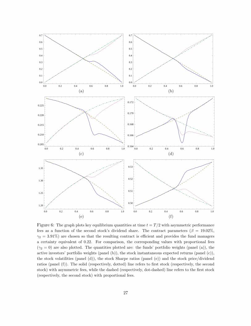
Moving now to equilibria in the presence of asymmetric performance fees, Figure 6 plotskey equilibrium quantities at time t = T/2 as a function of the second stock’s dividendshare. For the analysis in Figure 6, we select the contract parameters (β = 19.02% andγ2 = 3.91%) to correspond to those of the contract on the Pareto frontier in Figure 2giving the managers a certainty equivalent of 0.22. For comparison, Figure 6 also plots thecorresponding equilibrium values in an economy with purely proportional fees. It is is usefulto keep in mind for the following discussion that an increase in the dividend share of thesecond (non-benchmark) stock is associated with an increase in the difference between theprice of the non-benchmark stock and the price of the benchmark stock: thus, the funds’excess return over the benchmark portfolio, (Wm

t −δS1t )/Wm

0 , is a monotonically increasingfunction of the second stock’s dividend share, with the excess return being zero in Figure 6at a dividend share of about 58%.

While fulcrum fees unambiguously induce fund managers to tilt their portfolios towardthe benchmark stock, asymmetric performance fees can induce risk-averse fund managerseither to select portfolios having high correlation with the benchmark in an attempt to hedgetheir compensation, or to select portfolios having low correlation with the benchmark in anattempt to maximize the variance of the excess return of the managed portfolio over the

30Chen, Noronha and Singal interpret the asymmetry of the price effect as evidence against the hypoth-esis that the effect is due to downward-sloping demand curves and in favor of the alternative hypothesisthat the effect is due to increased investors’ awareness. Our analysis implies that portfolio delegation andbenchmarking is an alternative possible explanation for the asymmetry of the effect.

26

0.0 0.2 0.4 0.6 0.8 1.0

0.0

0.1

0.2

0.3

0.4

0.5

0.6

0.7

(a)0.0 0.2 0.4 0.6 0.8 1.0

0.0

0.1

0.2

0.3

0.4

0.5

0.6

0.7

(b)

0.0 0.2 0.4 0.6 0.8 1.0

0.205

0.210

0.215

0.220

0.225

(c)0.0 0.2 0.4 0.6 0.8 1.0

0.164

0.166

0.168

0.170

0.172

(d)

0.0 0.2 0.4 0.6 0.8 1.0

1.20

1.25

1.30

1.35

(e)0.0 0.2 0.4 0.6 0.8 1.0

0.50

0.51

0.52

0.53

(f)

Figure 6: The graph plots key equilibrium quantities at time t = T/2 with asymmetric performancefees as a function of the second stock’s dividend share. The contract parameters (β = 19.02%,γ2 = 3.91%) are chosen so that the resulting contract is efficient and provides the fund managersa certainty equivalent of 0.22. For comparison, the corresponding values with proportional fees(γ2 = 0) are also plotted. The quantities plotted are: the funds’ portfolio weights (panel (a)), theactive investors’ portfolio weights (panel (b)), the stock instantaneous expected returns (panel (c)),the stock volatilities (panel (d)), the stock Sharpe ratios (panel (e)) and the stock price/dividendratios (panel (f)). The solid (respectively, dotted) line refers to first stock (respectively, the secondstock) with asymmetric fees, while the dashed (respectively, dot-dashed) line refers to the first stock(respectively, the second stock) with proportional fees.

27

0.0 0.2 0.4 0.6 0.8 1.0

0.705

0.710

0.715

0.720

0.725

0.730

0.735

(a)

0.0 0.2 0.4 0.6 0.8 1.0

0.70

0.75

0.80

0.85

0.90

0.95

(b)

0.0 0.2 0.4 0.6 0.8 1.0

0.05

0.06

0.07

0.08

0.09

0.10

0.11

0.12

(c)

Figure 7: The graph plots the funds’ overall equity portfolio weight (panel (a), solid line), thefunds’ shares holdings (panel (b), solid and dotted lines) and the funds’ return and tracking errorvolatilities (panel (c), solid and dotted lines) with asymmetric performance fees as a function of thesecond stock’s dividend share. The contract parameters (β = 19.02%, γ2 = 3.91%) are chosen sothat the resulting contract is efficient and provides the fund managers a certainty equivalent of 0.22.For comparison, in panels (a) and (b) the corresponding values with proportional fees (γ2 = 0) arealso plotted.

28

benchmark (and hence the expected value of their performance fees, which are a convexfunction of this excess return). These shifting risk incentives are evident in panel (a) ofFigure 6, which plots the funds’ portfolio weights, or, even more clearly, in panel (a) ofFigure 7, which plots the funds’ share holdings. As shown in the figures, the first incentivedominates (inducing fund managers to tilt the fund portfolios toward the benchmark stock)when the fund’s excess return is positive or moderately negative (in Figures 6 and 7, whenthe second stock’s dividend share is larger than 56%, corresponding to an excess returnabove -6.2%), while the second incentive dominates (inducing fund managers to tilt thefund portfolios toward the non-benchmark stock) when the fund’s excess return is sufficientlynegative (below -6.2%).31 When the fund’s excess return is strongly negative, so that theprobability of earning positive performance fees is negligible, the fund managers essentiallybehave as if they were receiving a purely proportional fee and the difference between theholdings of the two stocks is close to zero. As shown in panel (b) of Figure 7, the overallequity allocation by mutual funds exceeds the overall allocation that would have been chosenwith purely proportional fees when the excess return is positive, has a small dip below thatlevel when the excess return is moderately negative, and converges to that level as the excessreturn become more and more negative.

As a result of the described portfolio strategy, the funds’ return volatility and trackingerror volatility are non-linear functions of the funds’ excess return, as shown in panel (c)of Figure 7. In particular, while tracking error volatility is decreasing in the fund’s excessreturn in the region where the funds’ excess return is between -22% and +6%, tracking errorvolatility is increasing in excess return outside of this region. This non-linear behavior isconsistent with the evidence on the risk-taking by mutual funds reported by Chevalier andEllison (1997) and Basak, Pavlova and Shapiro (2007). It is also interesting to note thatthe fund’s total return volatility is increasing in excess return in the region where the funds’excess return is between -60% and +32%, although the range is small (between 11.43%and 11.92%). This is consistent with the finding of a positive (although not statisticallysignificant) relationship by Busse (2001) and Basak, Pavlova and Shapiro (2007).32

The behavior of expected returns and Sharpe ratios in panels (c) and (e) of Figure 6reflects the behavior that could be expected to ensure market clearing given the fund man-agers’ portfolio strategy described above. In particular, the non-benchmark stock’s expectedreturn and Sharpe ratio are above (respectively, below) those of the benchmark stock in theregion in which the fund managers’ portfolios are tilted toward the benchmark (respectively,the non-benchmark) stock. Moreover, both stock’s expected returns and Sharpe ratios arebelow (respectively, above) the corresponding quantities in an economy with purely propor-

31Clearly, which incentive dominates at a given excess return critically depends on both the managers’risk aversion and the time horizon T . A less risk averse manager has stronger incentives to pick portfolioswith low correlation with the benchmark, in an attempt to maximize the variance of excess return over thebenchmark. A shorter time horizon has a similar effect.

32With fulcrum fees, the tracking error volatility is monotonically increasing in the excess return, whilethe return volatility is monotonically decreasing. Thus, a convex performance-based compensation is neededin order to generate the non-linearities described in the text. However, Brown, Harlow and Starks (1996),Chevalier and Ellison (1997) and Sirri and Tufano (1998) have documented that, even when mutual fundmanagers do not receive explicit incentive fees, an implicit nonlinear performance-based compensation stillarises with periodic proportional fees as a result of the fact that the net investment flow into mutual fundsvaries in a convex fashion as a function of recent performance.

29

0.2 0.4 0.6 0.8 1.0

0.0

0.1

0.2

0.3

0.4

0.5

0.6

0.7

(a)0.2 0.4 0.6 0.8 1.0

0.0

0.1

0.2

0.3

0.4

0.5

0.6

0.7

(b)

0.2 0.4 0.6 0.8 1.0

0.205

0.210

0.215

0.220

0.225

(c)0.2 0.4 0.6 0.8 1.0

0.164

0.166

0.168

0.170

0.172

(d)

0.2 0.4 0.6 0.8 1.0

1.20

1.25

1.30

1.35

(e)0.2 0.4 0.6 0.8 1.0

0.50

0.51

0.52

0.53

(f)

Figure 8: The graph plots key equilibrium quantities at time t = T/2 with asymmetric performancefees as a function of the second stock’s dividend share, immediately following an unanticipated changein the benchmark from stock 1 to stock 2. The contract parameters (β = 19.02%, γ2 = 3.91%) arechosen so that the resulting contract provides the fund managers a certainty equivalent of 0.22. Forcomparison, the corresponding values prior to the benchmark recomposition are also plotted. Thequantities plotted are: the fund managers’ portfolio weights (panel (a)), the active investors’ portfolioweights (panel (b)), the stock instantaneous expected returns (panel (c)), the stock volatilities (panel(d)), the stock Sharpe ratios (panel (e)) and the stock price/dividend ratios (panel (f)). The solid(respectively, dotted) line refers to first stock (respectively, the second stock) after the benchmarkrecomposition, while the dashed (respectively, dot-dashed) line refers to the first stock (respectively,the second stock) before the benchmark recomposition.

30

tional fees in the region in which the overall equity allocation by fund managers is above(respectively, below) that with purely proportional fees. Price/dividend ratios also havetheir expected behavior given their inverse relation to expected returns (panel (f)).

Perhaps surprisingly, equilibrium stock volatilities in the presence of asymmetric perfor-mance fees tend to be generally smaller than those in an economy with purely proportionalfees, in spite of the higher portfolio turnover.33 The reduction in volatilities is particu-larly strong in the region in which the funds’ performance is moderately positive (Figure 6,panel (d)): in fact, in this region the volatility of the first stock is not only lower than thecorresponding volatility in an economy with purely proportional fees, but also lower thanthan in the benchmark economy. The source of this volatility reduction can be understoodby noticing that, in the presence of asymmetric performance fees, the turnover by mutualfunds is concentrated in the region in which their excess return is moderately positive andis associated with a portfolio reallocation away from the stock whose dividend share (and,hence, whose price) is rising (Figure 7, panel (a)): to ensure market clearing (that is, toinduce active investors to hold even more of the stock whose dividend share is rising), theprice of stock must rise less than what it would have otherwise, lowering its volatility. Thesmall increase in volatilities over their values in an economy with purely proportional feescan be explained by a symmetric argument.

Turning now to the effect of changes in the composition of the benchmark portfolio,Figure 8 plots the key equilibrium quantities immediately before and after an unanticipatedchange at time t = T/2 in the benchmark from 100% stock 1 to 100% stock 2.

With asymmetric performance fees the effect of a benchmark change depends on funds’excess return, reflecting the fund managers’ portfolio allocation decisions described above.While it is difficult to distinguish this in panel (f) of Figure 8, in the region where funds’excess return is negative (respectively, below -12.4%), the price of the stock added to (re-spectively, deleted from) the index slightly decreases (respectively, increases), while theopposite behavior prevails for larger excess returns. These price effects are however muchsmaller than with fulcrum fees, the absolute percentage price change not exceeding 55 basispoints in the calibration in Figure 8. Sharpe ratios exhibit a similar pattern, with typicallyan opposite sign of the differential between pre- and post-recomposition values than the onefor prices.

Figures 6–8 were plotted for a single contract on the Pareto frontier in Figure 2. Bycontrast, Figure 9 shows how the key equilibrium quantities at time 0 vary as we con-sider different contracts on the Pareto frontier. As noted in Section 5, along this frontierhigher performance sensitivities γ2 are associated with higher managers’ certainty equiva-lents. Apart for the expected monotonic widening of the differentials across the two stocksassociated with larger performance sensitivities, the relationship between equilibrium quan-tities at time 0 plotted in Figure 9 and the performance sensitivity depends critically onthe endogenously-chosen allocation to mutual funds by fund investors in response to thevarying cost of portfolio management (as measured by the fund managers’ certainty equiv-alent). As the optimal performance sensitivity increases from 0% to 27%, reflecting anincrease in the fund managers’ equilibrium certainty equivalent from 0 to 0.28, the fundinvestors’ allocation to mutual funds decreases from 100% to 37% of their endowment. As

33Equilibrium strategies are buy-and-hold in the presence of purely proportional fees, while, as shown inpanel (a) of Figure 7, there is positive turnover in the presence of asymmetric performance fees.

31

0.00 0.05 0.10 0.15 0.20 0.25

0.26

0.28

0.30

0.32

0.34

0.36

0.38

0.40

(a)0.00 0.05 0.10 0.15 0.20 0.25

0.26

0.28

0.30

0.32

0.34

(b)

0.00 0.05 0.10 0.15 0.20 0.25

0.13

0.14

0.15

0.16

0.17

(c)0.00 0.05 0.10 0.15 0.20 0.25

0.134

0.136

0.138

0.140

0.142

(d)

0.00 0.05 0.10 0.15 0.20 0.25

0.95

1.00

1.05

1.10

1.15

(e)0.00 0.05 0.10 0.15 0.20 0.25

0.30

0.32

0.34

0.36

0.38

(f)

Figure 9: The graph plots key equilibrium quantities at time t = 0 with asymmetric performance feesas a function of the performance fee parameter γ2. The proportional fee parameter β is adjusted sothat the resulting contracts are efficient. For comparison, the corresponding values with proportionalfees (γ2 = 0) are also plotted. The quantities plotted are: the fund managers’ portfolio weights(panel (a)), the active investors’ portfolio weights (panel (b)), the stock instantaneous expectedreturns (panel (c)), the stock volatilities (panel (d)), the stock Sharpe ratios (panel (e)) and thestock price/dividend ratios (panel (f)). The solid (respectively, dotted) line refers to first stock(respectively, the second stock) with asymmetric fees, while the dashed (respectively, dot-dashed)line refers to the first stock (respectively, the second stock) with proportional fees.

32

a result of this quickly decreasing allocation to mutual funds, the number of shares of bothstocks held by mutual funds is a monotonically decreasing function of γ2 in spite of theincreasing proportional allocation to stocks by mutual funds. Hence, the active investors’proportional allocation to both stocks must be an increasing function of γ2, as shown inpanel (b) of Figure 9, leading to increasing expected returns and Sharpe ratios (panels (c)and (e)).

As shown in panel (a) of Figure 9, at time 0, when excess return is null, fund managers arein the region in which they find it optimal to tilt their portfolios toward the benchmark stock.This tilt is monotonic in the performance sensitivity parameter γ2. Therefore, equilibriumprices must adjust so that active investors are induced to tilt their portfolios toward the non-benchmark stock. As shown in panels (c)–(e), while the equilibrium expected return for thenon-benchmark stock exceeds that of the benchmark stock, this higher expected return isoffset by a higher volatility, resulting in the Sharpe ratio of the non-benchmark stock beingbelow that of the other stock. Therefore, at time 0, the equilibrium incentive for activeinvestors to tilt their portfolios toward the non-benchmark stock does not arise from thebenchmark stock having a higher Sharpe ratio or a lower volatility than the non-benchmarkstock, but from hedging considerations. To understand the source of this hedging demand,it is useful to refer back to Figures 6 and 7. Around the point corresponding to zero excessperformance for mutual funds (a dividend share around 58%), the total equity allocation bymutual funds is an increasing function of the dividend share and, to ensure market clearing,the Sharpe ratios of both stocks are decreasing functions of the dividend share. Thus, inthis region, active investors have positive hedging demand for the non-benchmark stock,whose price (being increasing in the stock’s dividend share) is negatively correlated withthe stocks’ Sharpe ratios and hence with the quality of the invest opportunity set.

6.4 Optimal Benchmarking

In order to clearly isolate the impact of delegated portfolio management on equilibriumprices, our numerical analysis has focused on the case in which the two liquidation dividendsare identically distributed and the benchmark portfolio is exogenously specified to be oneof the two stocks. However, in equilibrium the composition of the benchmark portfolioshould be determined endogenously and so we briefly address the robustness of our resultsto optimal benchmarking in the context of asymmetric performance fees.34

When optimally determining the composition of the benchmark, fund investors seek tomaximize the overall equity allocation by fund managers while at the same time minimizingthe investment distortions induced by benchmarking. In general, the portfolio held by fundmanagers is a (dynamically-rebalanced) combination of the market portfolio, the benchmarkportfolio and the riskless asset. Therefore, when the benchmark portfolio coincides with themarket portfolio of risky assets, the fund managers’ equilibrium trading strategy consistsof a combination of this portfolio and the riskless asset, eliminating the distortions in theallocation to risky assets induced by benchmarking and benefiting fund investors. On theother hand, because it is suboptimal in this case for fund managers to increase the trackingerror volatility of their portfolio (and hence the expected value of their performance fees) by

34Asymmetric performance fees dominate other fee structures within our piecewise linear class for allbenchmark choices.

33

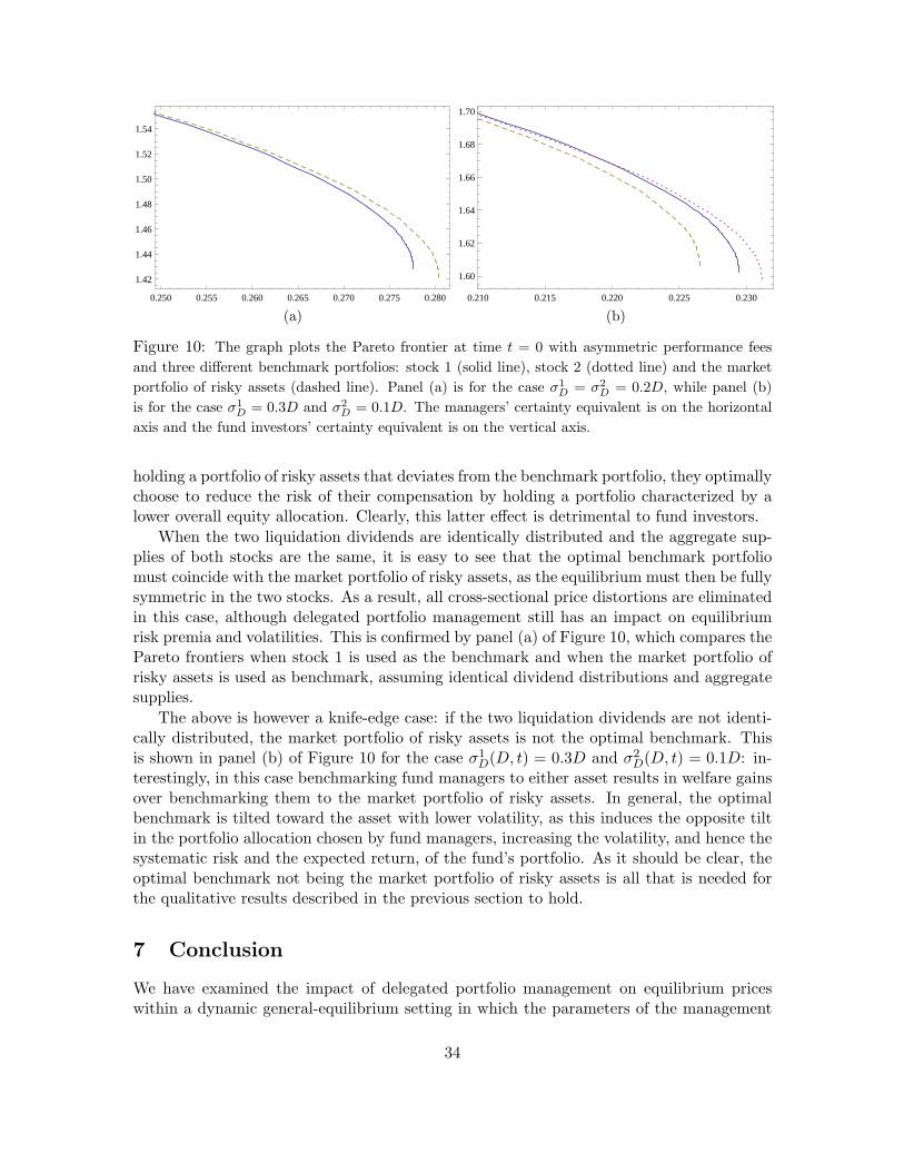
0.250 0.255 0.260 0.265 0.270 0.275 0.280

1.42

1.44

1.46

1.48

1.50

1.52

1.54

(a)0.210 0.215 0.220 0.225 0.230

1.60

1.62

1.64

1.66

1.68

1.70

(b)

Figure 10: The graph plots the Pareto frontier at time t = 0 with asymmetric performance feesand three different benchmark portfolios: stock 1 (solid line), stock 2 (dotted line) and the marketportfolio of risky assets (dashed line). Panel (a) is for the case σ1

D = σ2D = 0.2D, while panel (b)

is for the case σ1D = 0.3D and σ2

D = 0.1D. The managers’ certainty equivalent is on the horizontalaxis and the fund investors’ certainty equivalent is on the vertical axis.

holding a portfolio of risky assets that deviates from the benchmark portfolio, they optimallychoose to reduce the risk of their compensation by holding a portfolio characterized by alower overall equity allocation. Clearly, this latter effect is detrimental to fund investors.

When the two liquidation dividends are identically distributed and the aggregate sup-plies of both stocks are the same, it is easy to see that the optimal benchmark portfoliomust coincide with the market portfolio of risky assets, as the equilibrium must then be fullysymmetric in the two stocks. As a result, all cross-sectional price distortions are eliminatedin this case, although delegated portfolio management still has an impact on equilibriumrisk premia and volatilities. This is confirmed by panel (a) of Figure 10, which compares thePareto frontiers when stock 1 is used as the benchmark and when the market portfolio ofrisky assets is used as benchmark, assuming identical dividend distributions and aggregatesupplies.

The above is however a knife-edge case: if the two liquidation dividends are not identi-cally distributed, the market portfolio of risky assets is not the optimal benchmark. Thisis shown in panel (b) of Figure 10 for the case σ1

D(D, t) = 0.3D and σ2D(D, t) = 0.1D: in-

terestingly, in this case benchmarking fund managers to either asset results in welfare gainsover benchmarking them to the market portfolio of risky assets. In general, the optimalbenchmark is tilted toward the asset with lower volatility, as this induces the opposite tiltin the portfolio allocation chosen by fund managers, increasing the volatility, and hence thesystematic risk and the expected return, of the fund’s portfolio. As it should be clear, theoptimal benchmark not being the market portfolio of risky assets is all that is needed forthe qualitative results described in the previous section to hold.

7 Conclusion

We have examined the impact of delegated portfolio management on equilibrium priceswithin a dynamic general-equilibrium setting in which the parameters of the management

34

contract, the extent of delegated portfolio management and the returns of both benchmarkand non-benchmark securities are all determined endogenously.

When fund managers receive performance fees of the fulcrum type, they optimally chooseto tilt their portfolios towards stocks that are part of the benchmark: in equilibrium, thisresults in a significant positive price effect associated with the addition of a stock to thebenchmark and a smaller negative price effect associated a deletion. These implications areconsistent with empirical evidence regarding changes in the composition of the S&P 500index (the most widely used benchmark portfolio). Everything else being the same, we alsofind that benchmark stocks have lower expected returns, lower Sharpe ratios and highervolatilities than similar non-benchmark stocks.

With asymmetric performance fees, the composition of the portfolios selected by fundmanagers depends critically on the funds’ excess return. As a result, cross-sectional differ-ences between benchmark and non-benchmark stocks can have either sign, depending onthe funds’ performance relative to the benchmark. Interestingly, the presence of portfoliomanagers receiving asymmetric performance fees can stabilize prices by decreasing the equi-librium stock volatilities of both benchmark and non-benchmark stocks, although portfolioturnovers are higher with asymmetric fees.

Previous literature has typically taken asset returns and the level of delegated portfoliomanagement as given, analyzing managers’ portfolio choice decisions and deriving optimalcontracts. We have complemented this literature by analyzing the asset pricing implicationsof a prevalent parametric class of existing contracts, when the level of delegated portfoliomanagement is determined endogenously. We have also demonstrated that when full dele-gation is not exogenously imposed, performance contracts may be welfare-improving, evenwhen there is no asymmetric information and investors and fund managers have CRRApreferences with the same risk aversion coefficient.

35

Appendix

To simplify the notation, throughout this Appendix we frequently suppress the explicitdependence of quantities such as W , W1 and W2 on W b.

Proof of Lemma 1. Suppose first that β + γ1 6= 0 and consider the system of equations

u′(α+ βW ∗1 + γ1(W ∗1 − δW b))(β + γ1)= u′(α+ βW ∗2 + γ2(W ∗2 − δW b))(β + γ2)

u(α+ βW ∗1 + γ1(W ∗1 − δW b))= u(α+ βW ∗2 + γ2(W ∗2 − δW b))

+ u′(α+ βW ∗2 + γ2(W ∗2 − δW b))(β + γ2)(W ∗1 −W ∗2 )

(33)

in the unknowns (W ∗1 ,W∗2 ). Direct computation shows that the system has the unique

solution W ∗1 =

(1− η

c

) α−γ1δW b

β+γ1− η

(1− 1

c

)α−γ2δW b

β+γ2

η − 1

W ∗2 = W ∗1 +1c

(α− γ1δW

b

β + γ1− α− γ2δW

b

β + γ2

),

(34)

where η =(β+γ2β+γ1

)1− 1c . Moreover,

γ1δWb − α

β + γ1< W ∗1 < δW b < W ∗2 . (35)

Letting W (W b) =(γ1δW b−αβ+γ1

)+(as in equation (9)) and W1(W b) = (W ∗1 )+ (as in equa-

tion (13)), it follows from the above inequality that W ≤W1 < δW b.If W1(W b) > 0, it then immediately follows from the system (33) that equations (11)

and (12) are satisfied, with equality in equation (12)) and W2(W b) = W ∗2 , establishing thelemma for this case.

If, on the other hand, W1(W b) = 0, then W ∗1 ≤ 0 and it follows from equation (35) thatα− γ1δW

b > 0. Therefore, the function

f(W ) = u(α− γ1δWb)− u(α+ βW + γ2(W − δW b)) (36)

+ u′(α+ βW + γ2(W − δW b))(β + γ2)W

is well defined for W ≥W b and the existence of a solution W2(W b) > δW b to equation (11)is equivalent to the existence of a zero of f in (δW b,∞). Clearly, f is continuous and strictlydecreasing on [δW b,∞). Moreover,

f(δW b) = u(α− γ1δWb)− u(α+ βδW b) + u′(α+ βδW b)(β + γ2)δW b

> u(α− γ1δWb)− u(α+ βδW b)

+ u′(α+ βW ∗2 + γ2(W ∗2 − δW b))(β + γ2)δW b

36

= u(α− γ1δWb)− u(α+ βδW b)

+ u′(α+ βW ∗1 + γ1(W ∗1 − δW b))(β + γ1)δW b

≥ u(α− γ1δWb)− u(α+ βδW b) + u′(α− γ1δW

b)(β + γ1)δW b

> 0,

where the second (in)equality follows from the fact that u′ is decreasing and W ∗2 > δW b, thethird from the first equation in the system (33), the fourth from the fact that u′ is decreasingand W ∗1 < 0 and the last from the fact that the function u(α + βW + γ1(W − δW b)) isconcave in W . Similarly,

f(W ∗2 ) = u(α− γ1δWb)− u(α+ βW ∗2 + γ2(W ∗2 − δW b))

+ u′(α+ βW ∗2 + γ2(W ∗2 − δW b))(β + γ2)W ∗2= u(α− γ1δW

b)− u(α+ βW ∗1 + γ1(W ∗1 − δW b))+ u′(α+ βW ∗1 + γ1(W ∗1 − δW b))(β + γ1)W ∗1

≤ 0,

where the second equality follows from the second equation in the system (33), while theinequality follows from the concavity of the function u(α+βW +γ1(W −δW b)). Therefore,there exists a unique W2(W b) ∈ (δW b,W ∗2 ) such that f(W2(W b)) = 0, thus establishingthe existence of a unique solution to equation (11). The inequality in equation (12) followsfrom the fact that in this case we have

u′(F (W1(W b),W b))(β + γ1) ≤ u′(F (W ∗1 ,Wb))(β + γ1)

= u′(F (W ∗2 ,Wb))(β + γ2)

< u′(F (W2(W b),W b))(β + γ2),

where the first (in)equality follows from the fact that u′ is decreasing and W1(W b) ≥ W ∗1 ,the second from the first equation in the system (33), and the last from the fact that u′ isdecreasing and W2(W b) < W ∗2 .

Finally, suppose that β+γ1 = 0 and let W (W b) = 0 (as in equation (9)) and W1(W b) =0. With f(W ) defined as in equation (36), we then have

f(δW b) = u′(α)γ2δWb > 0.

Since2(α+ γ2(W − δW b))δW b

γ2(W − δW b)2→ 0 as W → +∞

and −Wu′′(W )/u′(W ) = c for all W , there exists a W ∗3 > δW b such that

2(α+ γ2(W ∗3 − δW b))δW b

γ2(W ∗3 − δW b)2< c

= − (α+ γ2(W ∗3 − δW b))u′′(α+ γ2(W ∗3 − δW b))u′(α+ γ2(W ∗3 − δW b))

,

or

u′(α+ γ2(W ∗3 − δW b))δW b +12u′′(α+ γ2(W ∗3 − δW b))γ2(W ∗3 − δW b)2 < 0. (37)

37

Moreover, since u′′′ > 0, it follows from a second-order Taylor expansion of the functionu(α+ γ2(W − δW b)) around the point W ∗3 that

u(α) < u(α+ γ2(W ∗3 − δW b))− u′(α+ γ2(W ∗3 − δW b))γ2(W ∗3 − δW b) (38)

+12u′′(α+ γ2(W ∗3 − δW b))γ2

2(W ∗3 − δW b)2.

Hence,

f(W ∗3 ) = u(α)− u(α+ γ2(W ∗3 − δW b)) + u′(α+ γ2(W ∗3 − δW b))γ2W∗3

< u′(α+ γ2(W ∗3 − δW b))γ2δWb +

12u′′(α+ γ2(W ∗3 − δW b))γ2

2(W ∗3 − δW b)2

< 0,

where the first inequality follows from equation (38), while the second follows from equa-tion (37). Therefore, f has a zero on (δW b,W ∗3 ), thus establishing the existence of a solutionto equation (11) in this case. The inequality in equation (12) is trivially satisfied, since theleft-hand side equals zero in this case.

Proof of Lemma 2. Equation (11) shows that v(·,W b) is continuous at W2(W b), whileequation (12) shows that v(·,W b) is continuously differentiable at W1(W b) if W1(W b) > 0(that is, if W1(W b) > W (W b)). It then immediately follows from the definition of vthat v(·,W b) is continuously differentiable and concave on [W (W b),∞). Moreover, sincev(W1(W b),W b) = u(F (W1(W b),W b)) and u(F (·,W b)) is strictly concave on the interval(W1(W b), δW b] while v(·,W b) is linear, it follows that v(·,W b) > u(F (·,W b)) on that inter-val. A similar argument implies that v(·,W b) > u(F (·,W b)) on the interval [δW b,W2(W b)).Since v(·,W b) = u(F (·,W b)) on A(W b), it follows that v(W,W b) ≥ u(F (W,W b)) on theinterval [W (W b),∞).

Finally, if v(·,W b) is any other concave function with v(·,W b) ≥ u(F (·,W b)) on the in-terval [W (W b),∞), then v(·,W b) ≥ u(F (·,W b)) = v(·,W b) onA(W b). Moreover, v(·,W b) ≥v(·,W b) on (W1(W b),W2(W b)) since v(W1(W b),W b) ≥ v(W1(W b),W b), v(·,W b) is concaveand v(·,W b) is linear on that interval. Therefore, v is the smallest concave function v(·,W b)with v(·,W b) ≥ u(F (·,W b))

Proof of Proposition 1. Standard optimization theory implies that a policy WT is opti-mal in the concavified problem (10) if and only if WT satisfies the conditions of Proposition 1with equation (14) replaced by the weaker condition

WmT ∈ v−1

W (ψmπT ,W bT ) if Wm

T > 0.

Thus, a policy WmT satisfying the conditions of Proposition 1 is optimal in the concavi-

fied problem (14). The fact that WmT takes values in A(W b

T ) implies u(F (WmT ,W

bT )) =

v(WmT ,W

bT ). Since u(F (·,W b

T )) ≤ v(·,W bT ), optimality of Wm

T in the concavified problem(10) then implies optimality in the original problem (8). This proves that the conditions inProposition 1 are sufficient for optimality.

38

Necessity follows immediately by noticing that if WT is any other feasible policy, then

E[u(F (WT ,W

bT ))]≤ E

[v(WT ,W

bT

)]≤ E

[v(WmT ,W

bT

)]= E

[u(F (Wm

T ,WbT ))],

with the first inequality being strict if WT 6∈ A(W bT ), and the second inequality being strict

otherwise.

Proof of Theorem 1. It can be easily verified that gm(y,W b, p) =(v−1W (y,W b)

)+for

y 6= vW (W2,Wb). The claim then immediately follows from Proposition 1.

Proof of Theorem 2. The proof of Theorem 2 is straightforward and is thus omitted.

Proof of Corollary 1. Under the stated assumptions, γ1 = γ2 and

α− γ1δWbT ≤ 0,

so thatΠ1(DT ,W

bT ) = Π3(DT ,W

bT ) ≥ Π4(DT ,W

bT ).

It then follows from equation (21), using the fact that β + γ1 = β + γ2 > 0, that

ψmπT = Π(DT ,WbT ) = Π1(DT ,W

bT ).

In addition, since by Lemma 2 W1 = W2 when γ1 = γ2, it follows from (16) and (17) that

WmT = gm(ψmπT ,W b

T , PT ) =Π1(DT ,W

bT )−

1c

(β + γ2)1− 1c

− α− γ2δWbT

β + γ2= θmT ·DT ,

where

θmT =ϕ(1− λ)γ2δθ

bT + (β + γ2)

1c θ −

(λ(β + γ2)

1c θf0 + ϕ(1− λ) αB

)θ1

λ(β + γ2)1c + ϕ(1− λ)(β + γ2)

It then immediately follows that the optimal trading strategy for the fund managers is asgiven in equation (28) for all t ∈ [0, T ]. The optimal trading strategy for the active investorsfollows from the market-clearing conditions.

Next, equation (25) implies that S1t − S2

t ≥ 0 if and only if

Et[Π1(DT ,W

bT )(D1

T −D2T )]≥ 0.

Let DT be two-dimensional random variable obtained from DT by exchanging the values ofD1T and D2

T . Since D1T and D2

T are identically distributed conditional on the informationat time t, we have

Et[Π1(DT ,W

bT )(D1

T −D2T )]

= Et[Π1(DT ,W

bT )(D1

T −D2T )1{D1

T>D2T }

]+ Et

[Π1(DT ,W

bT )(D1

T −D2T )1{D2

T>D1T }

]= Et

[Π1(DT ,W

bT )(D1

T −D2T )1{D1

T>D2T }

]+ Et

[Π1(DT ,W

bT )(D2

T −D1T )1{D1

T>D2T }

]= Et

[(Π1(DT ,W

bT )−Π1(DT ,W

bT ))

(D1T −D2

T )1{D1T>D

2T }

].

39

The claim regarding the equilibrium stock prices then easily follows from the fact that, whenγ2 6= 0 and D1

T > D2T , Π1(DT , θ

bT ) > Π1(DT , θ

bT ) (respectively, Π1(DT , θ

bT ) < Π1(DT , θ

bT ))

if and only if the benchmark portfolio θbT holds more (respectively, less) of stock 1 than ofstock 2.

40

References

Admati, A.R., and P. Pfleiderer, 1997 , “Does It All Add Up? Benchmarks and theCompensation of Active Portfolio Managers”, Journal of Business, 70, 323–350.

Allen, F., 2001, “Presidential Address: Do Financial Institutions Matter?”, Journal ofFinance, 56, 1165–1176.

Arora, N., N. Ju and H. Ou-Yang, 2006, “A Model of Asset Pricing under PortfolioDelegation and Differential Information”, working paper, University of North Carolina.

Aumann, R.J., 1966, “Existence of Competitive Equilibria in Markets with a Continuumof Traders”, Econometrica, 34, 1–17.

Aumann, R.J., and M. Perles, 1965, “A Variational Problem Arising in Economics”,Journal of Mathematical Analysis and Applications, 11, 488–503.

Bank for International Settlements, 2003, “Incentive Structures in InstitutionalAsset Management and their Implications for Financial Markets”, Report by the Committeeon the Global Financial System.

Basak, S., A. Pavlova, and A. Shapiro, 2007, “Optimal Asset Allocation and RiskShifting in Money Management”, Review of Financial Studies, forthcoming.

Beneish, M.D., and R.E. Whaley, 1996, “An Anatomy of the ‘S&P 500 Game’: TheEffect of Changing the Rules”, Journal of Finance, 51, 1909–1930.

Bhattacharya, S., and P. Pfleiderer, 1985, “Delegated Portfolio Management”, Jour-nal of Economic Theory, 36, 1–25.

Berk J.B., and R.C. Green, 2004, Mutual Fund Flows and Performance in RationalMarkets, Journal of Political Economy, 112, 1269–1295.

Brennan, M.J., 1993, “Agency and Asset Pricing”, working paper, UCLA.

Brown, K.C., W.V. Harlow, and L.T. Starks, 1996, “Of Tournaments and Temp-tations: An Analysis of Managerial Incentives in the Mutual Fund Industry”, Journal ofFinance, 51, 85–110.

Busse, J.A., 2001, “Another Look at Mutual Fund Tournaments”, Journal of Financialand Quantitative Analysis, 36, 53–73.

Cadenillas, A., J. Cvitanic and F. Zapatero, 2007, ”Optimal Risk Sharing withEffort and Project Choice”, Journal of Economic Theory, 133, 403–440.

Carpenter, J., 2000, “The Optimal Dynamic Investment Policy for a Fund ManagerCompensated with an Incentive Fee”, Journal of Finance, 55, 2311–2331.

Chen, H., G. Noronha, and V. Singal, 2004, “The Price Response to S&P 500 IndexAdditions and Deletions: Evidence of Asymmetry and a New Explanation”, Journal ofFinance, 59, 1901–1929.

Chen, H.-L., and G. Pennacchi, 2005, “Does Prior Performance Affect a Mutual Fund’sChoice of Risk? Theory and Further Empirical Evidence”, working paper, University ofIllinois at Chicago.

41

Chevalier, J., and G. Ellison, 1997, “Risk Taking by Mutual Funds as a Response toIncentives”, Journal of Political Economy, 105, 1167–1200.

Cochrane, J.H., F.A. Longstaff, and P. Santa-Clara, 2007 , “Two Trees”, Journalof Business, 80, 323–350.

Coles, J.L., J. Suay, and D. Woodbury, 2000 , “Fund Advisor Compensation inClosed-End Funds”, Journal of Finance, 55, 1385–1414.

Cornell, B., and R. Roll, 2005, “A Delegated-Agent Asset-Pricing Model”, FinancialAnalysts Journal, 61, 57–69.

Cox, J.C., and C.-F. Huang, 1989, “Optimal Consumption and Portfolio Policies whenAsset Prices Follow a Diffusion Process”, Journal of Economic Theory, 49, 33–83.

Cvitanic, J., X. Wan and J. Zhang, 2007, “Continuous-Time Principal-Agent Problemswith Hidden Action and Lump-Sum Payment”, working paper, Caltech.

Das, S., and R. Sundaram, 2001, “On the Regulation of Fee Structures in MutualFunds”, in M. Avellaneda (ed.), Quantitative Analysis in Financial Markets (v.3), CourantInstitute of Mathematical Sciences, New York.

Das, S., and R. Sundaram, 2002, “Fee Speech: Signaling, Risk-sharing and the Impactof Fee Structures on Investor Welfare,” Review of Financial Studies, 15, 1465–1497.

Del Guercio, D., and P.A. Tkac, 1998, “The Determinants of the Flow of Funds ofManaged Portfolios: Mutual Funds versus Pension Funds”, working paper, University ofOregon.

Del Guercio, D., and P.A. Tkac, 2002, “The Determinants of the Flow of Fundsof Managed Portfolios: Mutual Funds versus Pension Funds”, Journal of Financial andQuantitative Analysis, 37, 523–557.

Dybvig, P., H. Farnsworth, and J. Carpenter, 2006, “Portfolio Performance andAgency”, working paper, Washington University.

“Incentive Fees and Mutual Funds”, Journal of Finance, 58, 779–804.

Goetzmann, W., J. Jr. Ingersoll, and S.A. Ross, 2003, “High Water Marks andHedge Fund Management Contracts”, Journal of Finance, 58, 1685–1717.

Gomez, J.-P., and F. Zapatero, 2003, “Asset Pricing Implications of Benchmarking: ATwo-Factor CAPM”, The European Journal of Finance, 9 (4), 343–357.

Grinblatt, M., and S. Titman, 1989, “Adverse Risk Incentives and the Design of Per-formance Based Contracts”, Management Science, 35, 807–822.

Harris, L., 1989, “S&P 500 Cash Stock Price Volatilities”, Journal of Finance, 44, 1155–1175.

Harris, L., and E. Gurel, 1986, “Price and Volume Effects Associated with Changes inthe S&P 500 List: New Evidence for the Existence of Price Pressures”, Journal of Finance,41, 815–829.

Heinkel, R., and N.M. Stoughton, 1994, “The Dynamics of Portfolio ManagementContracts”, Review of Financial Studies, 7, 351–387.

42

Holstrom, B., and P. Milgrom, 1987, “Aggregation and Linearity in the Provision ofIntertemporal Incentives”, Econometrica, 55, 303–328.

Hugonnier, J., and R. Kaniel, 2006, “Mutual Fund Portfolio Choice in the Presence ofDynamic Flows”, working paper, Duke University.

Kapur, S., and A. Timmermann, 2005, “Relative Performance Evaluation Contracts andAsset Market Equilibrium”, Economic Journal, 115, 1077–1102.

Kihlstrom, R., 1988, “Optimal Contracts for Security Analysts and Portfolio Managers”,Studies in Banking and Finance, 5, 291–325.

Larsen, K., 2005, “Optimal Portfolio Delegation when Parties Have Different Coefficientsof Risk Aversion”, Quantitative Finance, 5, 503–512.

Liu, W.-L., 2005, “Motivating and Compensating Investment Advisors”, Journal of Busi-ness, 78, 2317–2349.

Lynch, A., and R. Mendenhall, 1997, “New Evidence on Stock Price Effects Associatedwith Changes in the S&P 500 Index”, Journal of Business, 70, 351–384.

Lynch, A., and D. Musto, 2003, How Investors Interpret Past Fund Returns, Journal ofFinance, 58, 2033–2058.

Ou-Yang, H., 2003, “Optimal Contracts in Continuous-Time Delegated Portfolio Manage-ment Problem”, Review of Financial Studies, 16, 173–208.

Palomino, F., and A. Prat, 2003, “Risk Taking and Optimal Contracts for MoneyManagers”, RAND Journal of Economics, 34, 113–137.

Pruitt, S.W., and K.C.J., Wei, 1989, “Institutional Ownership and Changes in theS&P 500”, Journal of Finance, 44, 509–513.

Roll, R., 1992, “A Mean/Variance Analysis of Tracking Error”, Journal of Portfolio Man-agement, 18, 13–22.

Ross, S.A., 1973, “The Economic Theory of Agency: The Principal’s Problem”, AmericanEconomic Review, 63, 134–139.

Ross, S.A., 2004, “Compensation, Incentives, and the Duality of Risk Aversion and Risk-iness”, Journal of Finance, 59, 207–225.

Shapley, L.S., and M. Shubik, 1965, “Quasi-Cores in a Monetary Economy with Non-Convex Preferences”, The Rand Corporation, RM-3518-1-PR.

Shleifer, A., 1986, “Do Demand Curves for Stocks Slope Down?”, Journal of Finance,41, 579–590.

Sirri, E., and P. Tufano, 1998, “Costly Search and Mutual Fund Flows”, Journal ofFinance, 53, 1589–1622.

Starks, L.T., 1987, “Performance Incentive Fees: An Agency Theoretic Approach”, Jour-nal of Financial and Quantitative Analysis, 22, 17–32.

Stoughton N.M., 1993, “Moral Hazard and the Portfolio Management Problem”, Journalof Finance, 48, 2009–2028.

43

Stracca, L., 2006, “Delegated Portfolio Management: A Survey of the Theoretical Liter-ature”, Journal of Economic Perspectives, 20, 823–848.

Wurgler, J., and E. Zhuravskaya, 2002, Does Arbitrage Flatten Demand Curves forStocks?, Journal of Business, 75, 583–608.

44