Embed Size (px)
Citation preview

Can preferential concentration of finite-size particles in planeCouette turbulence be reproduced with the aid of
equilibrium solutions?T. Pestana∗
Aerodynamics Group, Faculty of Aerospace EngineeringTechnische Universiteit Delft
Kluyverweg 2, 2629 HS Delft, The Netherlands
Markus Uhlmann†Insititute for Hydromechanics,
Karlsruhe Insititute of Technology,Karlsruhe, 76131, Germany
Genta Kawahara‡Graduate School of Engineering Science,
Osaka University, 1-3 Machikaneyama, Toyonaka,Osaka 560-8531, Japan
Friday 14th February, 2020(accepted for publication in Phys. Rev. Fluids (2020))
AbstractThis work employs for the first time invariant solutions of the Navier-Stokes equations to
study the interaction between finite-size particles and near-wall coherent structures. We con-sider horizontal plane Couette flow and focus on Nagata’s upper-branch equilibrium solution(Nagata, 1990) at low Reynolds numbers where this solution is linearly stable. When addinga single heavy particle with a diameter equivalent to 2.5 wall units (one twelfth of the gapwidth), we observe that the solution remains stable and is essentially unchanged away fromthe particle. This result demonstrates that it is technically feasible to utilize exact coherentstructures in conjunction with particle-resolved DNS. While translating in the streamwisedirection, the particle migrates laterally under the action of the quasi-streamwise vorticesuntil it reaches the region occupied by the low-speed streak, where it attains a periodic stateof motion – independent of its initial position. As a result of the ensuing preferential par-ticle location, the time-average streamwise particle velocity differs from the plane-averagefluid-phase velocity at the same wall-distance as the particle center, as previously observedin experiments and in numerical data for fully turbulent wall-bounded flows. Additional con-strained simulations where the particle is maintained at a fixed spanwise position while freelytranslating in the other two directions reveal the existence of two equilibria located in thelow-speed and in the high-speed streak, respectively, the former being an unstable point. Aparametric study with different particle to fluid density ratios is conducted which shows howinertia affects the spanwise fluctuations of the periodic particle motion. Finally, we discuss anumber of potential future investigations of solid particle dynamics which can be conductedwith the aid of invariant solutions (exact coherent structures) of the Navier-Stokes equations.
∗[email protected]†[email protected]‡[email protected]
1
arX
iv:2
002.
0436
1v2
[ph
ysic
s.fl
u-dy
n] 1
2 Fe
b 20
20

1 IntroductionIn many natural and technical systems the interaction between fluid flow and solid particles playsan important role. Examples are the most diverse: in nature it ranges from blood flow to volcaniceruptions, whereas in industrial applications a classical example is the combustion of pulverizedcoal. In such systems, one aspect that is of primordial importance is the spatial distributionof the dispersed phase. It can significantly affect various quantities of practical interest, suchas particle dispersion, inter-particle collision statistics, mean relative velocities and turbulenceenhancement/attenuation. Nevertheless, to the present day, our understanding of the fundamentalprocess behind structure formation in the particulate phase or about turbulence modulation dueto particles is still incomplete.
A typical approach to understand fluid-particle interaction consists of analyzing data fromdirect numerical simulations (DNS). These analyses are often performed a posteriori and consistin operations like spatial filtering or conditional averaging in an attempt to extract the key mecha-nisms that govern fluid-particle interaction. Approaches of this kind have led to new observationsand have advanced the knowledge on this topic quite considerably in the past decades. For ex-ample, in wall-bounded flows, heavy particles moving near a solid wall tend to concentrate in thelow-speed regions and form streamwise aligned streaks. This particle preferential concentrationhas been observed in numerous experimental and numerical investigations, (e.g., Refs. (Garcıa-Villalba et al., 2012, Hetsroni & Rozenblit, 1994, Kaftori et al., 1995, Nino & Garcia, 1996, Pan& Banerjee, 1997, Rashidi et al., 1990, Uhlmann, 2008, Yung et al., 1989)), and it is knownto depend on particle size and density. Kidanemariam et al. (2013) performed particle-resolvedDNS of horizontal turbulent channel flow with a very dilute set of particles having a diameterequivalent to 7 wall units and a submerged weight which essentially restricted them to a posi-tion in contact with the lower bounding wall. Through conditional averaging they found thatthere is a significant statistical correlation between spanwise particle velocity and the presence ofa nearby quasi-streamwise vortex with the corresponding sign of rotation. This statistical argu-ment explains the migration to low-speed streaks which are typically flanked by counter-rotatingstreamwise vortices; as a consequence, the average streamwise particle velocity is lower than themean fluid velocity at the same wall-distance due to the preferential particle concentration in low-speed regions. Despite the success of such statistical approaches it is not always straightforwardto extract the salient features of a fully turbulent flow field from massive DNS data-sets, and tolink the relevant flow structures to the observed particle dynamics.
An alternative to the above methods is to consider surrogate flow-fields instead of fully-developed turbulence. This has the obvious advantage of making the analysis of particle motionconceptually easier, although at the risk of being less relevant to the fully turbulent state of inter-est. Along this line, Maxey (2002) used a cellular flow to investigate the clustering properties ofsmall spherical particles, and Reeks et al. (2006) considered randomized Taylor-Green vortex flowto elucidate the random uncorrelated particle motion. Of equal interest is the work of Bergoug-noux et al. (2014), who set up experimentally a cellular flow to investigate the influence of vorticalstructures upon the settling of small particles.
Another way to simplify the problem, which has to the best of our knowledge not yet beenexplored, is to investigate particle motion in flow fields that are invariant solutions to the Navier-Stokes equations. These solutions are widely believed to be of relevance to full turbulence, as someof them are able to reproduce statistical features of turbulent flows; cf. Kawahara et al. (2012)for a review about the significance of invariant solutions to turbulence, and van Veen (2019) for areview on the history of invariant solutions in turbulence. Invariant solutions range from simplefixed points (equilibrium states), which are time invariant in some suitable frame of reference, tomore complex and dynamic flow fields that recur at a fixed time period (periodic orbits). Solutionsof this type have been found in various flow configurations, such as plane Couette flow (Nagata,1990), plane Poiseuille flow (Waleffe, 2001), Hagen-Poiseuille flow (Faisst & Eckhardt, 2003), orsquare-duct flow (Okino et al., 2010, Uhlmann et al., 2010). In the present contribution we focuson plane Couette flow, which on one hand is a wall-bounded flow with far-reaching applications,and for which, on the other hand, well-known solutions exist.
2

Equilibrium states for plane Couette flow have traditionally been found through homotopytechniques, i.e. by embedding the problem of interest into a generalized configuration: Nagata(1990) used spanwise rotation, Clever & Busse (1992) resorted to wall heating, and Waleffe (1998)imposed an artificial body force. Nagata’s solution originates from a saddle-node bifurcation ata finite Reynolds number, and it can be continued along a lower and an upper solution branch,both of which extend to high-Reynolds numbers. The upper branch of the solution is believed tobe of relevance for the turbulent state: the coherent structures embedded therein, i.e. a pair ofcounter-rotating streamwise vortices flanking a wavy low-speed streak, emulate well the coherentstructures typically found in the turbulent buffer layer, and the velocity profiles of these solutionsalso resemble those typically found in turbulent wall-bounded flows (Jimenez et al., 2005). Let usmention in passing that periodic orbits containing a full regeneration cycle of vortices and velocitystreaks have been detected in plane Couette flow by Kawahara & Kida (2001) and others.
Thus, some of the known invariant solutions, more specifically equilibrium solutions, provideexact coherent structures that are of relevance to turbulence, like an apparatus in a laboratorythat would contain some of the main ingredients of turbulence (Kerswell, 2005), albeit typicallyat low Reynolds number. This unique trait is appealing for the study of the effects of coherentvortices on particle dynamics, as it makes the problem more amenable by untangling turbulenceand isolating its building blocks. However, this approach is technically not trivial as the presenceof a solid phase can disturb the equilibrium state and lead to re-laminarization or transition toturbulence. In a first step towards introducing the concepts of invariant solutions into the studyof finite-size particle motion, the present work considers the question whether simple invariantsolutions seeded with finite-size particles can be used to study the interaction between finite-sizeparticles and true turbulence. To this end, we address the following specific questions in thecontext of plane Couette flow:
(i) How long can equilibrium solutions be observed once finite-size particles have been added?
(ii) Do equilibrium solutions seeded with finite-size particles exhibit preferential particle concen-tration?
In Section 2 we describe the flow configuration, present the numerical methodology, and define thephysical and numerical parameters of this study. In the sequence (Section 3), we compute a setof equilibrium solutions and study their stability. Finally, in Section 4, we add finite-size particlesto these plane Couette flow equilibria and study the ensuing temporal evolution of the system.
2 Numerical Set-up2.1 Flow configuration and parametersWe consider plane Couette flow with two parallel walls, which are separated by a distance 2h,and extend in the x and z directions by Lx and Lz, such that the physical domain is definedas Ω = [0,Lx] × [−h, h] × [0,Lz] (cf. Fig. 1). The walls move in the x-direction with speed U ,and their counter movement induces shear and drives the flow. A gravitational field g acts in thenegative wall normal direction with intensity g.
The fluid motion is governed by the incompressible Navier-Stokes equations, viz.
∇ · uf = 0, (1)
∂uf∂t
+ (uf · ∇) uf = − 1ρf∇p+ ν∇2uf , (2)
where, uf = (uf , vf , wf ) is the fluid velocity, p is the hydrodynamic pressure, ν is the kinematicviscosity of the fluid and t denotes time. The flow field uf satisfies a no-slip boundary conditionat the two solid walls and at the fluid/particle interface. The flow field is assumed periodic in thex and z directions with streamwise and spanwise wavelengths λx = Lx and λz = Lz, respectively.
3

The motion of the solid-phase, which is formed of finite-size spherical particles of diameter Dp
and density ρp, is governed by the Newton-Euler equations for the motion of rigid bodies:
ρpVpdupdt = ρf
∮
∂S
τ · n dσ + (ρp − ρf )Vpg, (3)
Ipdωpdt = ρf
∮
∂S
r× (τ · n)dσ. (4)
Here up = (up, vp, wp) is the linear particle velocity, ωp is the angular particle velocity, τ =−p I+2ν(uf +uTf ) is the hydrodynamic stress with I the identity tensor and r the position vectorwith respect to the particle’s centroid. The vector normal to the fluid-solid interface ∂S is denotedby n, and the volume and the moment of inertia of the particles are Vp and Ip, respectively. Atthe fluid/particle interface ∂S, a no-slip boundary condition is imposed through an immersedboundary method as further explained in Section 2.2.3 and in Appendix A. Particle-wall contactis assumed to be frictionless, as in the DNS of Kidanemariam et al. (2013). Particles can, therefore,slide without additional tangential stress along the horizontal walls.
In its most general form, our numerical experiments involve a total of 9 control parametersthat need to be prescribed: ρp, ρf , ν,Lx,Lz, h,Dp, U, g. This specific set may be combinedinto a group of 6 independent non-dimensional numbers. These are taken as the dimensionlessgeometrical dimensions Lx/h and Lz/h, the Reynolds number based on the absolute wall speedand on half of the wall separation Re = Uh/ν, the density ratio ρp/ρf , the non-dimensionalparticle diameter Dp/h and the Galileo number Ga = ugDp/ν, where ug =
√(ρp/ρf − 1)gDp is
the gravitational velocity.The box-averaged energy dissipation rate ED, is defined as
ED = h2
U2 〈ωf · ωf 〉xyz, (5)
where ωf denotes the fluid vorticity, and 〈 · 〉xyz is the spatial average over the three spatialdirections. Note that the dissipation defined in (Eq. (5)) is normalized such that the laminar flowsolution yields ED = 1. The instantaneous wall shear stress, averaged over each of the two wallplanes, is defined as:
τw,l = ρfν∂〈uf 〉xz∂y
∣∣∣y=−h
and τw,u = ρfν∂〈uf 〉xz∂y
∣∣∣y=+h
(6)
where 〈 · 〉xz denotes the two-dimensional spatial averaging operator. By defining the mean frictionvelocity as uτ =
√(τw,l + τw,u)/(2ρf ), the viscous lengthscale is given by δν = ν/uτ , and the
friction-velocity-based Reynolds number is Reτ = uτh/ν. Henceforth the standard notation witha “+” superscript refers to quantities normalized with these viscous wall units. The bulk velocityis defined as
ub = 1h
∫ h
0〈uf 〉xz(y) dy , (7)
which lets us define a bulk flow time scale τb = h/ub.The responsiveness of particles to fluid forcing is typically measured through the Stokes number,
i.e. the ratio between particle and fluid time scales. Taking the particle response time based onthe Stokes drag τp = D2
pρp/(18νρf ), we define a first Stokes number based on bulk time unitsStb = τp/τb and a second Stokes number St+ = τp/τν based on the viscous time-scale τν = δν/uτ .
Spatial fluctuations of flow quantities around the wall-parallel plane average are defined asfollows, e.g. for the fluid velocity: u′f = uf − 〈uf 〉xz. From these we define second moments suchas the box-averaged kinetic energy of the fluctuations K = 〈u′f ·u′f 〉xyz/2, and the plane-averagedvelocity variances, e.g. in the streamwise direction 〈u′fu′f 〉xz. We will also employ time-averagingwhich is indicated through the use of the operator 〈 · 〉t with the averaging interval being mademore precise below.
4

2.2 Numerical methodsThe numerical approach employed in this study involves three different methodologies based onseparate code frameworks. First, we use a Newton-Raphson solver to find equilibrium solutionsof the Navier-Stokes equations in plane Couette flow. Second, the stability of the equilibriumstates are tested with the aid of a pseudo-spectral DNS solver. Third, a DNS finite-difference codecoupled with the Newton/Euler equations of rigid particle motion is employed for time marchingequilibrium solutions seeded with finite-size particles. In the following we briefly describe thedifferent numerical methods.
2.2.1 Equilibrium solutions
Equilibrium solutions are solenoidal velocity fields ueqf that satisfy the condition ∂ueqf /∂t = 0 inEq. (2) for a given Re, λx and λz. The present methodology is essentially equivalent to the one ofEhrenstein & Koch (1991) which uses the Laplacian of the wall-normal velocity perturbation andthe wall-normal vorticity perturbation as unknowns, and which employs Fourier series expansionsand Chebyshev polynomials for the spatial discretization. The resulting non-linear set of equationsis solved iteratively through a Newton-Raphson method. In order to track solutions in the Re,λx and λz parameter space, an arc-length continuation method is employed (Keller, 1977). Thenumerical code used in this part of the study is the same as used in Jimenez et al. (2005), and werefer the reader to the latter reference for more details.
2.2.2 Stability analysis
In order to investigate the stability of equilibrium solutions (in the absence of solid particles)we perform a time-stepping-based stability analysis where white noise is added to ueqf , and thedisturbed velocity field is advanced in time by a pseudo-spectral DNS code. If the disturbancesare amplified in time, the parameter point is regarded as unstable. On the other hand, if thedisturbances are damped in time, the parameter point is considered stable. The white noise thatis added to each degree of freedom is of the form A exp(Iθ), where I is the unit imaginary number,θ ∈ [0, 2π] is a random phase and A is the amplitude of the disturbance. The employed numericalalgorithm is as described by Kim et al. (1987). It solves the governing equations using againa pressure-free formulation, where the dependent variables are the Laplacian of the wall-normalvelocity and the wall-normal vorticity. The unknowns are expanded with Fourier/Chebyshevseries, and a three-step low-storage Runge-Kutta scheme is used for time integration. The code isessentially the same as the one used in Jimenez & Pinelli (1999) with slight modifications for theCouette flow boundary conditions.
2.2.3 Interface-resolved particulate flow solver
In order to solve the set of equations (Eq. (1)-Eq. (4)) for the coupled motion of fluid and parti-cles we resort to an immersed boundary technique. A body force term f ibm is introduced on theright-hand-side of the momentum equation (Eq. (2)) which is formulated such that the no-slip con-dition is enforced at the particle surface. The specific formulation is the one proposed by Uhlmann(2005) which is reproduced in appendix Appendix A for convenience. A standard fractional stepmethod is employed, and the spatial gradients are discretized through central, second-order finite-differences on a staggered mesh. The temporal discretization is performed with a Crank-Nicolsonscheme for the viscous terms and a three-step Runge-Kutta scheme for advection. The parti-cle motion (Eq. (3)-Eq. (4)) is explicitly coupled to the solution of the Navier-Stokes equations(Eq. (1)-Eq. (2)). The Poisson equation for the pseudo-pressure is solved with the aid of a multi-grid technique; the Helmholtz problems for the velocity prediction are solved with an approximatefactorization technique. The numerical code uses three-dimensional Cartesian domain decomposi-tion for parallelism on distributed memory systems. The particle-wall interaction is treated witha simple repulsive force method (Glowinski et al., 1999), as in the DNS study of Kidanemariam
5

et al. (2013); no tangential (frictional) contact force is imposed. For the two-phase flow simula-tions the computational grid is uniform and isotropic due to requirements for consistency of theimmersed boundary method. This condition is however relaxed for the single-phase simulations.The numerical algorithm is described in detail in Uhlmann (2005) and has been used in a numberof previous studies, e.g. (Chouippe & Uhlmann, 2015, Kidanemariam et al., 2013, Uhlmann, 2008,Uhlmann & Doychev, 2014).
3 Tracking Equilibrium SolutionsBefore considering particulate flows, we need to establish the relevant single-phase equilibriumsolutions as well as their stability properties.
3.1 Nagata’s solutionsWe restrict our search to Nagata-like solutions as these have been extensively studied in theliterature. We consider solutions with different values of the Reynolds number Re, and withdifferent fundamental wavenumbers λx and λz. For this purpose we use two different computationaldomains Ω1 and Ω2, the latter one being twice as large in both the streamwise and the spanwisedirection (cf. Tab. 1).
First we have continued one of Nagata’s solutions previously used in Jimenez et al. (2005) withrespect to the fundamental wavelengths λx and λz until it matched the size of the target domainsΩ1 and Ω2. Then continuation in terms of Re was performed with 16×32×16 Fourier-Chebyshev-Fourier coefficients, and equilibrium states of interest were recomputed with 48×49×48 coefficients(112 896 degrees of freedom). We have verified that this numerical resolution is sufficient to resolvethe highest coefficients of the Fourier-Chebyshev-Fourier representation up to machine precisionfor all Re numbers that are considered here.
The average dissipation rate of the single-phase flow solutions is shown in Fig. 2 for both setsof fundamental wavenumbers. It can be observed that for these parameters, the branches originateat the critical Reynolds number 171.45 (128.61) in domain Ω1 (Ω2). The upper branches featuresubstantially larger values of the dissipation rate which indicates the presence of finer scales, i.e.steeper spatial velocity gradients. Note that many previous authors have computed Nagata-typesolutions for plane Couette flow (e.g. Gibson et al., 2009, Waleffe, 2003); however, we re-computedthem here for convenience and for having precise control over the cell size. In the following wefocus upon equilibrium solutions on the upper-branch, as they are directly related to the turbulentstate (Jimenez et al., 2005), as further discussed in Section 3.3.
3.2 Stability analysisIn order to determine the stability of the equilibrium solutions, we added white noise with anamplitude A = 10−5 U (cf. Section 2.2.2). Each of these perturbed solutions were integrated intime using the pseudo-spectral time-stepper, and, in total, we analyzed 10 (6) parameter pointson the upper-branch of domain Ω1 (Ω2). The stability of each parameter point was judged basedon the box-averaged kinetic energy of the fluctuations. Note that the superscript “ps” indicatesa quantity computed with the aid of the pseudo-spectral time-stepper, whereas the unperturbedkinetic energy is denoted as Kps
ref . The cases in which the perturbation caused the system tomove away from its equilibrium value were regarded as unstable, and otherwise as stable. As anexample, Fig. 3(a) shows an unstable parameter point leading to the laminar state, and Fig. 3(b)shows a stable one. Our analysis reveals that all the investigated parameter points of domainΩ1 are unstable, whereas the upper-branch of domain Ω2 is stable within a narrow Re region inthe proximity of the turning point. The results of this stability analysis are summarized by theshaded areas in Fig. 2, and the specific results are documented in Appendix B. Although, we didnot perform a sensitivity study by varying the amplitude of the initial perturbation, we have alsoapplied the same procedure to successfully reproduce the results of Clever & Busse (1997). In that
6

study, the authors show that the upper-branch of Nagata’s solutions with (λx, λz) = (4πh, 2πh)is indeed stable for Re in the vicinity of Remin.
Note that the above analysis does not take into account possible instability with respect tosub-harmonic perturbations, since we perform the DNS in a domain which is commensurate withthe fundamental harmonic of Nagata’s solution (i.e. with Lx = λx and Lz = λz).
3.3 Characteristics of the selected equilibrium solutionFor the remainder of this work we select as our principle parameter point the solution at Re =132.25 on the upper branch of domain Ω2 (cf. Tab. 2 for precise values of the physical parameters).
In order to provide insight into the structure of the chosen single-phase flow field, we showin Fig. 4(a) iso-surfaces of the Q-criterion of Hunt et al. (1988) colored according to the sign ofstreamwise vorticity, plotted alongside iso-surfaces of the streamwise velocity. It can be seen thata wavy low-speed streak is flanked by counter-rotating vortices resembling the coherent structurestypically found in near-wall turbulence. These features are present despite the low value of thefriction Reynolds number Reτ = 15.87.
The corresponding wall-normal profiles of the mean streamwise velocity and of the standarddeviations of velocity (all with respect to the wall-parallel plane average) for this solution areshown in Fig. 4(b,c). It can be seen that these low-order moments of the velocity field exhibit thequalitative features of their statistical counterparts found in turbulent flows (Bech et al., 1995),e.g. a representative anisotropy and a distinct peak of the streamwise fluctuation intensity.
4 Exact Coherent Structures and Finite-Size ParticlesLet us now turn to the main part of this work by adding finite-size particles to the previouslyselected single-phase solutions. Particles are inserted into the fluid domain with their initialvelocity set equal to that of the unperturbed fluid at the initial position of the particle’s centroid.In total, we have conducted 15 independent simulations with physical parameters as listed inTab. 3. While the particle diameter is set to Dp/h = 0.156 (D+
p = 2.48) throughout this work, weconsider a range of density ratios ρp/ρf in order to explore the effect of particle inertia.
The chosen number of grid nodes is 768 × 128 × 384 except where stated otherwise. Theuniform isotropic grid spacing is therefore equivalent to ∆x+ = ∆y+ = ∆z+ = 0.25 which in turncorresponds to a particle resolution of Dp/∆x = 10. Note that we have checked that the resultsdo not change significantly when refining the grid by a factor of 2/3, i.e. with a grid comprising1152× 193× 576 nodes and a particle resolution of Dp/∆x = 15. Details on this refinement studyare presented in Appendix D.
4.1 Single particleLet us first consider case S10 which features a single particle with density ratio ρp/ρf = 10,corresponding to a wall-unit-based Stokes number of St+ = 3.41.
The particle is released at an arbitrary position in the vicinity of the bottom wall, after whichthe simulation is run for a total duration of Tobs = 1500 τb. Based on the resulting data we cannow address the main questions laid out in the introduction of this study: does the presence ofa single-particle disturb the equilibrium solution significantly? Does the particle motion exhibitpreferential concentration with respect to the coherent flow structures?
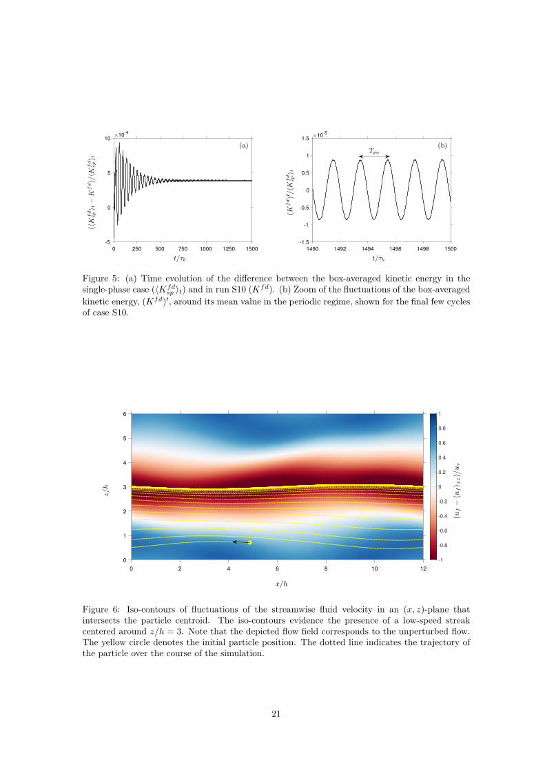
Remarkably, it turns out that the presence of the finite-size solid particle does not disfigure theequilibrium state, and Nagata’s solution is surprisingly well preserved even after 1500 τb. First, inFig. 5a we compare the time evolution of kinetic energy in case S10 with the corresponding resultsfrom the single-phase simulation (Fig. 13). Here the reference single-phase solution is representedby its time averaged value in the interval 300 < t/τb < 350, 〈Kfd
sp 〉t (where the subscript “sp” wasadded to denote single-phase). It is observed that the signal exhibits a damped oscillation whichdecays on the order of O(103) bulk time units, finally yielding a sinusoidal periodic signal (cf.
7

Fig. 5b). The period of the signal in the asymptotic state is Tpo = 2.04 τb, and the amplitude of itsfluctuations only measures approximately 10−5 times the mean kinetic energy of the unperturbedflow field, 〈Kfd
sp 〉t. The discrepancy in the mean value of kinetic energy induced by the presenceof the single particle is marginal and on the order of 10−4〈Kfd
sp 〉t, thus indicating that Nagata’ssolution is essentially preserved at this parameter point. This observation is also confirmed byflow visualization, which yields largely consistent structures as in the single-phase case (cf. Fig. 4),and which has therefore been omitted here. A refined analysis shows that the introduction ofthe particle triggers a very slight unsteadiness of the macroscopic flow field, which correspondsto Nagata’s solution moving in the negative x-direction with a tiny propagation velocity equal to−2.33 · 10−4ub. This result has been verified under the above mentioned grid refinement.
Let us now turn to the particle dynamics. We observe that the particle moves in the (negative)streamwise direction at roughly the speed of the surrounding fluid. Due to the action of thespanwise velocity induced by the quasi-streamwise vortices, it slowly drifts towards the spanwisecenter of the domain, approaching the low-speed fluid region (cf. Fig. 6). Meanwhile, the wall-normal motion of the particle is insignificant, and it remains near its initial wall-normal positionduring the course of the simulation, as expected from its large Galileo number value. By followingthe particle’s spanwise position (Fig. 7), we observe that it takes about 50 τb for the particle toreach the region occupied by the low-speed streak (around zp/h = 3). Subsequently, the spanwiseparticle position attains a state with a purely sinusoidal oscillation with amplitude 0.09h andperiod Tp = 3.93 τb, as can be seen from the inset in Fig. 7. The average streamwise particle velocitymeasures 〈up〉ft = −0.94U , and the time for one particle flow-through (Lx/〈up〉ft) matches withthe period of the spanwise oscillatory motion Tp.
As a consequence of the preferential location of the particle in the low-speed streak, it turnsout that the time-average particle velocity in the asymptotic state significantly differs from thecorresponding average fluid velocity. Let us define an apparent velocity lag as follows
ulag = 〈uf 〉xz(y = −h+D/2)− 〈up〉ft . (8)
Here we obtain a value of ulag = 1.1uτ which is comparable to what has been observed in DNSof turbulent horizontal channel flow by Kidanemariam et al. (2013): these authors’ particles withdiameter D+ = 7 in a flow with Reτ = 185 exhibited an apparent velocity lag of approximately2uτ when located in the immediate vicinity of the wall. Let us underline that the apparent lag doesnot reflect the relative velocity seen by the particle, but that it is a consequence of the separateaveraging of each phase in equation (Eq. (8)), and, therefore, that it reflects the statistical biasdue to preferential particle concentration.
It is also noteworthy that the mechanism of particle migration is caused by the spanwise flowvelocity induced by the quasi-streamwise vortices. Consequently the spanwise particle motion isessentially due to the hydrodynamic drag force which can be modeled by standard quasi-steadydrag formulae (Clift et al., 1978). It should then in principle be possible to obtain a fair repro-duction of the present results in the context of a point-particle approach, i.e. without resolvingthe flow around the suspended rigid particle (Balachandar & Eaton, 2010), and to use the presentset-up as a testbed for such models. It appears worthwile to further explore this avenue in futurestudies.
4.2 Multiple particlesIn order to check the dependency of our results upon the particle position at its time of release,we have simulated the temporal evolution starting from various initial values. For reasons ofefficiency, we have done these tests in a multi-particle simulation (case M10 in Tab. 3), where 10particles are simultaneously released at random positions in the wall-parallel plane in the vicinityof the lower wall (cf. Fig. 8). The evolution of the spanwise position, which is shown in Fig. 9,reveals that the spanwise motion in the asymptotic state is harmonic with the same period andamplitude for all particles. The latter matches well with the values found in the single-particlecase S10, demonstrating two points: first, that particles migrate towards the low-speed streak
8

irrespective of their initial position, and, second, that collective effects are not felt at this lowparticle concentration. Therefore, this multi-particle simulation confirms the observation that thepersistent low-speed streak acts as a stable attractor to near-wall particle motion.
4.3 Constrained particlesWhile dynamical simulations (as the ones which we have presented above) can be used for thedetection of stable equilibria of the system, it is not easy to find possible unstable equilibria withthis method. Furthermore, it is of general interest to determine the stability properties of particlelocations with respect to the coherent structures of the background flow in more detail. In order toobtain such additional information, it is useful to resort to the method of constrained simulations,where some otherwise dynamical quantity is held fixed, while the applied constraining force (ortorque) is measured. This approach has been successfully used e.g. by Patankar et al. (2001) andby Joseph & Ocando (2002) for the investigation of the wall-normal migration of neutrally-buoyantparticles in wall-bounded shear flows.
In the present context we proceed as follows. We seed the equilibrium solution with parti-cles whose motion in the spanwise direction is suppressed, while they are free to move in thestreamwise/wall-normal plane. We then let the simulation evolve until an asymptotic state isreached, which now features the particle translating on an essentially straight path (in the x-direction) in a time-periodic regime of motion, during which the hydrodynamic force acting uponthe particles oscillates with the same period. The force component in the constraining directionat a given spanwise position, Fz(z, t), is our primary quantity of interest. In case of a steady statesystem, the equilibria are then readily obtained as the positions ze where the force Fz(ze) van-ishes; stability (instability) can be detected by checking for negative (positive) gradients ∂Fz/∂zat the equilibrium positions. In the present case, where the constraining force is time-dependent,we perform the same analysis for the time-average of the spanwise component of the particleforce, 〈Fz(z, t)〉t. It should be noted that this is clearly a simplification, as the effect of temporalfluctuations upon the stability of the spanwise particle position are thereby effectively ignored.Therefore, this point might merit further investigation in future studies.
In case C10 (with otherwise same parameters as cases S10 and M10, cf. Tab. 3) we perform aconstrained simulation with 10 particles simultaneously (again for reasons of efficiency). In orderto minimize their mutual influence, we initially place the particles uniformly on a diagonal in the(x, z)-plane. This numerical set-up was integrated in time for 116 τb, which corresponds to morethan 20 passages through the domain. However, we have verified that the forces acting on theparticles already attain their asymptotic time evolution after only two of these passages, afterwhich the values fluctuate by less than 5% from passage to passage. The time-average spanwiseforce 〈Fz〉t acting on the particles (in the asymptotic regime) is shown in Fig. 10 as a function of therespective spanwise position. As expected, the force exhibits two zero-crossings at ze/h = 3, 6.One equilibrium position coincides with a positive gradient of the spanwise force (ze/h = 6), andit can therefore be classified as unstable; the other one (ze/h = 3), which coincides with the meanlocation of the low-speed streak, is stable, since the gradient of 〈Fz〉t is negative at that position.
Therefore, this simplified analysis confirms that the low-speed region is the only stable equi-librium for the particles’ spanwise location. Please note that this constrained simulation is signif-icantly more efficient than the unconstrained one, since the transient time interval to be coveredis much shorter. The present results consequently underline that the constrained simulation ap-proach is a very useful tool in the context of computationally demanding resolved-particle DNS.
4.4 Density ratioIn order to elucidate the scaling of the particle mobility as a function of its inertia, we havevaried the solid-to-fluid density ratio by a factor of twenty from case S04 to S80 (cf. Tab. 3),while maintaining all remaining physical and numerical parameters fixed (the Stokes and Galileonumbers vary accordingly). Please note that here we strictly separate the inertia effect from the
9

geometrical size effect by keeping the particle diameter fixed. This is fundamentally different fromvarying the Stokes number in the context of a point-particle approach.
In all runs, the initial position of the particle is the same as in case S10, and the simulationsare carried out for 110 τb. After their initial release, all cases display similar dynamics as case S10(as already shown in Fig. 7), and the time for the particles to reach the low-speed streak does notappear to depend significantly on the density ratio ρp/ρf (figure omitted). Note that in all casesthe particle remains in contact with the lower wall at all times, except for a short initial transientat the lowest Galileo number case S04. At later times, all runs exhibit a sinusoidal periodic motionin the (x, z)-plane, analogous to case S10, as can be seen from Fig. 11. In the asymptotic state,the particles oscillate around the same time-average position 〈zp〉t/h = 3, irrespective of theirdensity ratio. The amplitude and the phase of the particle motion, however, vary monotonouslywith ρp/ρf . More specifically, these amplitudes (Az for the spanwise particle excursions, and Awfor the spanwise particle velocity fluctuations) are defined as one half of the difference betweenmaximum and minimum values of the data shown in Figs. 11a and 11b, respectively. Fig. 12 thenshows that over the investigated parameter range both amplitudes (spanwise particle position andvelocity) first decrease roughly linearly with the density ratio, and then exhibit an increasinglynon-linear evolution with ρp/ρf . This behavior can be qualitatively explained with the aid ofvery simple point-particle arguments, invoking Stokes drag to be the only particle force actingin the spanwise direction and assuming that the velocity seen by the particle is the unperturbedflow velocity of the equilibrium solution. Under these assumptions the amplitude of the spanwiseparticle excursions and of its spanwise velocity fluctuations decays as (ρp/ρf )−1 for large densityratios. However, in order to allow for a quantitative match with the data for finite-size particles,a more elaborate model would be required, taking into account unsteady force terms, finite-sizeand finite-Reynolds number corrections as well as wall effects. Again, the formulation of a realisticforce model in the context of a point-particle approach would be a rewarding subject for futureresearch, for which the present configuration can serve as a useful validation case.
5 Conclusions and perspectives for further studiesIn this work we have attacked the problem of fluid-particle interaction with the aid of particle-resolved DNS based on an immersed-boundary method. Instead of considering turbulent flowand performing statistical analysis we have used a non-trivial equilibrium solution which featuresexact coherent structures (streaks and vortices) representative of the principal ingredients of wall-bounded shear flows. The present strategy has the advantage of a much reduced complexity, inparticular in terms of ease of data-analysis.
More specifically, we have focused here on the upper branch of Nagata’s solution for planeCouette flow, which has previously been shown to reproduce some of the low-order statisticsof the turbulent flow state. For the present work we have restricted our attention to a lowReynolds number, for which the single-phase flow solution is stable to finite-amplitude white noiseperturbations. We have found that adding either a single or a small number of heavy sphericalparticles with a diameter equivalent to one twelfth of the gap width (2.5 wall units) does notsignificantly alter the flow structure, such that the background flow is essentially maintained. Atthe same time, a solid particle, which due to gravity remains in a plane adjacent to the lowerhorizontal wall, migrates towards the region occupied by a low-speed streak, and then attainsa regime of periodic motion which is independent of the initial position. As a consequence ofthe particle’s preferential location, it does not sample the flow field uniformly, and, therefore, itstime-average velocity differs from the (unperturbed) mean flow velocity at the wall-distance of itscentroid.
This apparent velocity lag has previously been reported in experiments and in DNS studies ofhorizontal channel flow in the turbulent regime. Although past studies have already laid out theabove mechanism leading to preferential particle concentration and its consequences, the data-analysis (involving coherent structure eduction and particle-conditioned statistical averaging) hasrequired much effort. When using exact coherent structures as the background flow, this effort
10

is significantly reduced. Furthermore, the technique of simulating constrained particles in orderto determine the stability properties of particle motion can be applied to flow fields which areinvariant solutions to the Navier-Stokes equations, as has been demonstrated in the present work.
Several new physical results have been obtained here by performing a sweep of the solid-to-fluiddensity ratio (ρp/ρf = 4 . . . 80 corresponding to St+ = 1.4 . . . 27). It turns out that the time ittakes for the particle to migrate to the equilibrium position (inside the low-speed streak) does notsignificantly depend on the particle density in the range under investigation. In the asymptoticregime, on the other hand, the effect of particle inertia leads to the amplitude of the oscillationsof the spanwise particle motion to decrease non-linearly with particle density.
To sum up, the present work demonstrates that it is technically feasible and beneficial to studyinvariant solutions (and in particular equilibrium solutions) with suspended finite-size particles.This set-up provides a numerical laboratory with minimal complexity, yet still relevant to the fullproblem of sustained turbulence. We expect the proposed approach to be fruitful in future studieson various aspects of particulate flow, and some perspectives for future work are briefly discussedin the following.
The most immediate avenue to pursue is to expand the study in parameter space. First, we notethat in the present contribution we have not varied the particle diameter. It is obviously of interestto determine the limit for the occurrence of the preferential location mechanism as the particlesize increases with respect to the scale of the coherent structures. Varying particle diameter anddensity independently will help to distinguish between relative size effects and inertial effects,as an alternative to the amalgamation of both in form of the Stokes number. Other importantparameters which are straightforward to investigate in this framework include the role of gravity(sweep of Galileo number, orientation of the vector of gravitational acceleration), as well as aninvestigation of collective effects.
One important aspect which merits further analysis is the consideration of parameter pointsat which the equilibrium solution as such is already unstable (e.g. Nagata’s upper branch solutionat larger Reynolds number). Preliminary computations indicate that the present approach stillmakes sense, as long as the solution remains suitably close to the equilibrium point over an intervalwhich is long compared to the particle’s characteristic time scale. For some parameter points itis expected that the presence of particles adds to the de-stabilization of the flow. The studyof the precise mechanisms by which particles contribute to the enhancement (or attenuation) ofinstability can be a rewarding subject by itself. Along these lines, we expect that the study ofinvariant solutions and finite-size particles can make a valuable contribution to the elucidationof open questions in the area of transition to turbulence in particulate flows (Loisel et al., 2013,Matas et al., 2003).
Since steady equilibrium solutions, such as the one considered herein, as well as other traveling-wave type solutions do not involve a notion of characteristic life-time of the coherent structures(i.e. the streaks and vortices are always present), possible effects of disparity of proper timescales in the fluid/particle interaction problem are not represented in this system. Therefore, itwould be of great value to consider time-periodic invariant solutions (i.e. periodic orbits) in futurestudies involving solid particles. Prime candidates in this direction are the periodic solutions forplane Couette flow discovered by Kawahara & Kida (2001), which feature a self-sustaining cycleinvolving velocity-streak break-up and regeneration of quasi-streamwise vortices. At the presenttime, however, it is not clear whether it will be feasible to conduct numerical experiments involvingfinite-size particles suspended in such periodic orbit solutions.
Finally, let us mention that the present approach can obviously be extended to the study ofsmall particles whose near-field does not need to be resolved (i.e. idealized as point particles).If the disperse phase is sufficiently dilute, the point-particle study can be conducted in one-waycoupled fashion (i.e. the perturbation of the fluid phase can be neglected), which then renders thenumerical simulations extremely efficient. Preliminary simulations of this type indicate that theywill yield interesting information on preferential concentration and clustering. In addition, we seean opportunity to validate and eventually improve force models in the context of the point-particleapproach with the aid of the present set-up. Such a study would have the clear advantage of fullreproducibility. Further elaboration of this topic will be left for future work.
11
AcknowledgmentsThe simulations were partially performed at SCC Karlsruhe. The computer resources, technicalexpertise and assistance provided by this center are thankfully acknowledged.
ReferencesBalachandar, S. & Eaton, J. 2010 Turbulent dispersed multiphase flow. Ann. Rev. Fluid
Mech. 42, 111–133.
Bech, K. H., Tillmark, N., Alfredsson, P. H. & Andersson, H. I. 1995 An investigationof turbulent plane couette flow at low Reynolds numbers. J. Fluid Mech. 286, 291âĂŞ325.
Bergougnoux, L., Bouchet, G., Lopez, D. & Guazzelli, E. 2014 The motion of solidspherical particles falling in a cellular flow field at low Stokes number. Physics of Fluids 26 (9),093302.
Chouippe, A. & Uhlmann, M. 2015 Forcing homogeneous turbulence in direct numerical sim-ulation of particulate flow with interface resolution and gravity. Physics of Fluids 27 (12),123301.
Clever, R. M. & Busse, F. H. 1992 Three-dimensional convection in a horizontal fluid layersubjected to a constant shear. Journal of Fluid Mechanics 234, 511.
Clever, R. M. & Busse, F. H. 1997 Tertiary and quaternary solutions for plane Couette flow.Journal of Fluid Mechanics 344, 137.
Clift, R., Grace, J. & Weber, M. 1978 Bubbles, drops and particles. Academic Press.
Ehrenstein, U. & Koch, W. 1991 Three-dimensional wavelike equilibrium states in planePoiseuille flow. Journal of Fluid Mechanics 228, 111.
Faisst, H. & Eckhardt, B. 2003 Traveling Waves in Pipe Flow. Physical Review Letters 91 (22),224502.
Garcıa-Villalba, M., Kidanemariam, A. G. & Uhlmann, M. 2012 DNS of vertical planechannel flow with finite-size particles: Voronoi analysis, acceleration statistics and particle-conditioned averaging. International Journal of Multiphase Flow 46, 54–74.
Gibson, J., Halcrow, J. & Cvitanovic, P. 2009 Equilibrium and travelling-wave solutions ofplane couette flow. J. Fluid Mech. 638, 243âĂŞ266.
Glowinski, R., Pan, T.-W., Hesla, T. & Joseph, D. 1999 A distributed Lagrange multi-plier/fictitious domain method for particulate flows. International Journal of Multiphase Flow25 (5), 755–794.
Hetsroni, G. & Rozenblit, R. 1994 Heat transfer to a liquid-solid mixture in a flume. Inter-national Journal of Multiphase Flow 20 (4), 671–689.
Hunt, J., Wray, A. & Moin, P. 1988 Eddies, streams, and convergence zones in turbulentflows. In Proceedings of the Summer Programm, pp. 193–208. (Center for Turbulence Research,Stanford).
Jimenez, J., Kawahara, G., Simens, M. P., Nagata, M. & Shiba, M. 2005 Characterizationof near-wall turbulence in terms of equilibrium and ”bursting” solutions. Physics of Fluids 17 (1),015105.
Jimenez, J. & Pinelli, A. 1999 The autonomous cycle of near-wall turbulence. Journal of FluidMechanics 389, 335–359.
12

Joseph, D. & Ocando, D. 2002 Slip velocity and lift. J. Fluid Mech. 454, 263–286.
Kaftori, D., Hetsroni, G. & Banerjee, S. 1995 Particle behavior in the turbulent boundarylayer. II. Velocity and distribution profiles. Physics of Fluids 7 (5), 1107–1121.
Kawahara, G. & Kida, S. 2001 Periodic motion embedded in plane Couette turbulence: Re-generation cycle and burst. Journal of Fluid Mechanics 449, 291–300.
Kawahara, G., Uhlmann, M. & van Veen, L. 2012 The Significance of Simple InvariantSolutions in Turbulent Flows. Annual Review of Fluid Mechanics 44 (1), 203–225.
Keller, H. B. 1977 Numerical Solution of bifurcation and nonlinear eigenvalue problems. InApplications of Bifurcation Theory, pp. 359–384. Academic Press.
Kerswell, R. 2005 Recent progress in understanding the transition to turbulence in a pipe.Nonlinearity 18, R17–R44.
Kidanemariam, A. G., Chan-Braun, C., Doychev, T. & Uhlmann, M. 2013 Direct nu-merical simulation of horizontal open channel flow with finite-size, heavy particles at low solidvolume fraction. New Journal of Physics 15 (2), 025031.
Kim, J., Moin, P. & Moser, R. 1987 Turbulence statistics in fully developed channel flow atlow Reynolds number. J. Fluid Mech. 177, 133–166.
Loisel, V., Abbas, M., Masbernat, O. & Climent, E. 2013 The effect of neutrally buoyantfinite-size particles on channel flows in the laminar-turbulent transition regime. Phys. Fluids25 (12), 123304.
Matas, J.-P., Morris, J. & Guazzelli, E. 2003 Transition to turbulence in particulate pipeflow. Phys. Rev. Lett. 90 (1), 014501.
Maxey, M. R. 2002 The motion of small spherical particles in a cellular flow field. Physics ofFluids 30 (7), 1915.
Nagata, M. 1990 Three-dimensional finite-amplitude solutions in plane Couette flow: bifurcationfrom infinity. Journal of Fluid Mechanics 217, 519.
Nino, Y. & Garcia, M. H. 1996 Experiments on particleâĂŤturbulence interactions in thenearâĂŞwall region of an open channel flow: implications for sediment transport. Journal ofFluid Mechanics 326, 285.
Okino, S., Nagata, M., Wedin, H. & Bottaro, A. 2010 A new nonlinear vortex state insquare-duct flow. J. Fluid Mech. 657, 413–429.
Pan, Y. & Banerjee, S. 1997 Numerical investigation of the effects of large particles on wall-turbulence. Physics of Fluids 9 (12), 3786–3807.
Patankar, N., Huang, P., Ko, T. & Joseph, D. 2001 Lift-off of a single particle in Newtonianand viscoelastic fluids by direct numerical simulation. J. Fluid Mech. 438, 67–100.
Rai, M. & Moin, P. 1991 Direct simulation of turbulent flow using finite-difference schemes. J.Comput. Phys. 96, 15–53.
Rashidi, M., Hetsroni, G. & Banerjee, S. 1990 Particle-turbulence interaction in a boundarylayer. International Journal of Multiphase Flow 16 (6), 935–949.
Reeks, M. W., Fabbro, L. & Soldati, A. 2006 In Search of Random Uncorrelated ParticleMotion (RUM) in a Simple Random Flow Field. In Volume 1: Symposia, Parts A and B, , vol.2006, pp. 1755–1762. ASME.
13
Roma, A., Peskin, C. & Berger, M. 1999 An adaptive version of the immersed boundarymethod. J. Comput. Phys. 153, 509–534.
Uhlmann, M. 2005 An immersed boundary method with direct forcing for the simulation ofparticulate flows. Journal of Computational Physics 209 (2), 448–476.
Uhlmann, M. 2008 Interface-resolved direct numerical simulation of vertical particulate channelflow in the turbulent regime. Physics of Fluids 20, 053305.
Uhlmann, M. & Doychev, T. 2014 Sedimentation of a dilute suspension of rigid spheres atintermediate Galileo numbers: the effect of clustering upon the particle motion. Journal of FluidMechanics 752, 310–348.
Uhlmann, M., Kawahara, G. & Pinelli, A. 2010 Travelling-waves consistent with turbulence-driven secondary flow in a square duct. Phys. Fluids 22 (8), 084102.
van Veen, L. 2019 A Brief History of Simple Invariant Solutions in Turbulence. In ComputationalModelling of Bifurcations and Instabilities in Fluid Dynamics, , vol. 50, pp. 217–231.
Waleffe, F. 1998 Three-Dimensional Coherent States in Plane Shear Flows. Physical ReviewLetters 81, 4140–4143.
Waleffe, F. 2001 Exact coherent structures in channel flow. Journal of Fluid Mechanics 435,93–102.
Waleffe, F. 2003 Homotopy of exact coherent structures in plane shear flows. Phys. Fluids15 (6), 1517–1534.
Yung, B. P., Merry, H. & Bott, T. R. 1989 The role of turbulent bursts in particle re-entrainment in aqueous systems. Chemical Engineering Science 44 (4), 873–882.
14

A Algorithm of the immersed boundary methodFor each time step which advances the solution from tn to tn+1 we perform three Runge-Kuttasub-steps with indices κ = 1, 2, 3. The fractional step method first computes a pre-predictedvelocity field u which does not include any explicit effect of the suspended particles. Next a forcefield f (ibm) is computed which serves to impose the desired no-slip velocity at the particle surfaces.The momentum equations are then solved with the added force field to yield a predicted velocityfield u∗. Subsequently a Poisson equation is solved for the pseudo-pressure φ which then servesto project the velocity field upon the divergence-free space, yielding the final field u. The particleequations of motion are finally updated to yield the new positions and particle velocities.
The overall algorithm for a single Runge-Kutta sub-step with index κ can be written as follows:
u = uκ−1 + ∆t2ακν∇2uκ−1 − 2ακ∇pκ−1 − γκ ((u · ∇)u)κ−1 − ζκ ((u · ∇)u)κ−2,(9a)
Uβ(X(m)l ) =
∑
ijk
uβ(x(β)ijk) δh(x(β)
ijk −X(m)l (tκ−1)) ∆x3 , ∀ l; m; β (9b)
F(X(m)l ) =
U(d)(X(m)l , tκ−1)− U(X(m)
l , tκ−1)∆t , ∀ l; m (9c)
f(ibm),κβ (x(β)
ijk) =Np∑
m=1
NL∑
l=1Fβ(X(m)
l ) δh(x(β)ijk −X(m)
l (tκ−1)) ∆V (m)l , ∀β; i; j; k (9d)
∇2u∗ − u∗
ακν∆t = − 1νακ
(u∆t + f (ibm),κ
)+∇2uκ−1 , (9e)
∇2φ = ∇ · u∗
2ακ∆t , (9f)
uκ = u∗ − 2ακ∆t∇φ , (9g)pκ = pκ−1 + φ− ακ∆t ν∇2φ , (9h)
uκ, (m)p − uκ−1, (m)
p
∆t = ρfVp(ρp − ρf )
−Fκ, (m) +
∑
l 6=mFκ−1, (l,m)rep + Fκ−1, (m)
wall
+ 2ακg , ∀m (9i)
xκ, (m)p − xκ−1, (m)
p
∆t = ακ
(uκ, (m)p + uκ−1, (m)
p
), ∀m (9j)
ωκ, (m)p − ωκ−1, (m)
p
∆t = − ρfρp − ρf
1(Ip/ρp)
T κ, (m) , ∀m (9k)
where m is the index of a given particle (1 ≤ m ≤ Np), β denotes a spatial direction (1 ≤ β ≤ 3),X(m)l is the position of a Lagrangian force point with index l (where 1 ≤ l ≤ Nl) attached to the
mth particle, δh is the discrete delta function of Roma et al. (1999), x(β)ijk is the position vector of a
node of the staggered Cartesian fluid grid of the velocity component in the xβ direction with indextriplet “ijk”, Uβ is the velocity in the xβ-direction interpolated to a Lagrangian position, U(d)(Xl)is the solid body velocity of the Lagrangian force point, F(X(m)
l ) is the immersed boundary forceat a Lagrangian force point, ∆V (m)
l is the forcing volume associated to the lth Lagrangian forcingpoint of the mth particle (equal to ∆x3 here), xκ, (m)
p is the centroid position of the mth particle,Fκ, (m) is the hydrodynamic force computed from the sum of the immersed boundary contributionsof the mth particle, T κ, (m) is the analogous hydrodynamic torque contribution, Fκ−1, (l,m)
rep andFκ−1, (m)wall are the force contributions from particle-particle and particle-wall contact, respectively.
The set of coefficients αk, γk, ξk for a low-storage scheme leading to second-order temporal accuracyhas been given in Rai & Moin (1991). Please refer to the original publication Uhlmann (2005) formore details on the algorithm.
15

B Stability analysisThe stable/unstable parameter points of the upper-branch of Nagata’s solutions for domains Ω1and Ω2 were previously summarized in form of shaded areas in the (Re, ED) state-space dia-gram (Fig. 2). Here, we list the discrete Re and ED values for which the stability analysis wasperformed — see Tab. 4.
In Tab. 4, the reader also finds the stable/unstable parameters points for a third domain,namely Ω3 = [0, 4πh] × [−h, h] × [0, 2πh]. Domain Ω3 is identical to the one used in Clever &Busse (1997), where the authors conducted a linear stability analysis. The reproduction of theirresults served to validate our stability analysis approach, which is instead based on a time-stepperapplied to an initial field which is perturbed by white noise, as detailed in Section 2.2.2. Inall cases, we restrict our analysis to parameter points located on the upper-branch of Nagata’ssolutions, as these are physically more interesting for the purpose of the current work.
C Computing single-phase equilibrium solutions with a finite-difference method
Here we wish to verify how closely the finite-difference solution on a given grid resembles thereference spectral results in the absence of particles. The equilibrium solution obtained withthe Newton-Raphson approach and spectral-discretization is first spectrally interpolated uponthe finite-difference grid, before starting time-stepping. Fig. 13 depicts the temporal evolutionof kinetic energy for the stable parameter point (cf. Tab. 2) when using 384 × 128 × 192 gridpoints, which implies a grid resolution of (∆x+,∆y+,∆z+) = (0.50, 0.25, 0.50). The figure showsthat the initial difference between Kfd and Kps (i.e. the error due to spatial interpolation witha second-order method) is less than 0.01Kps. In Fig. 13 a mild temporal evolution in the formof a low-amplitude damped oscillation is subsequently observed for the finite-difference solution,which converges to within 0.7% discrepancy of the spectral reference data.
D Grid convergence study for case S10Here we compare the main findings of case S10 with results from case S10-F which features arefined grid. For this additional run, the number of grid points was increased by a factor of3/2 yielding 1152×193 × 576 nodes, i.e. ∆x+ = ∆y+ = ∆z+ = 0.167, and a particle resolutionof Dp/∆x = 15. The remaining numerical and physical parameters were held constant and arereadily found in Tab. 3.
The initial condition for case S10-F was taken from the state of the system in case S10 att = 820.50 τb. The respective velocity field was first interpolated on the finer grid and the sim-ulation was subsequently continued until t = 1500 τb. The interpolation introduced disturbancesin the former steady flow-field and gave rise to a new transient, as evidenced by the discontinuityin the time evolution of box-averaged kinetic energy in case S10-F shown in Fig. 14. The tran-sient behavior is, as before, marked by a damped oscillation, which decays in time and slowlyapproaches a periodic state. The time-average of (Kfd) differs by 0.3% of Kps(t = 0) betweenthe computations on the two grids. Despite the lengthy time integration, we observe that thewell-defined periodic motion previously seen in Fig. 5b is not yet fully established in case S10-F(see the inset in Fig. 14), whereas the signature of the periodic motion is already clearly developed.Note that the remaining slow modulation at the end of the simulation S10-F has an amplitudeof approximately 1.5 times the amplitude of the oscillations related to the flow-through of theparticle. The period of the latter oscillations in case S10-F measures Tpo ≈ 1.94 τb which is inclose agreement with case S10 (cf. Fig. 5b); for the amplitude of the fluctuations we observe adiscrepancy of approximately 7% between the two grids.
Concerning the spanwise particle motion in the asymptotic regime, we find a good agreementbetween the results obtained with the two grids (S10 and S10-F) for the particle position (Fig. 15a)
16
and velocity (Fig. 15b). For both signals, case S10-F exhibits amplitudes that are lower by 11%than in case S10. The shapes of the curves, however, remain unaltered, and re-scaling the spanwisevelocity of the finer case recovers the signal of the coarser run. This confirms the negligible phase-lag between the two curves in Fig. 15.
17

Table 1: Geometrical dimensions of the plane Couette numerical set-up used to compute Na-gata’s equilibrium solutions. The half wall separation is given by h and an illustration of thecomputational domain is shown in Fig. 1.
Domain ID Lx/h Lz/h λx/h λz/hΩ1 6 3 6 3Ω2 12 6 12 6
Table 2: Physical parameters of the stable equilibrium solution selected to study the interactionbetween finite-size particles and exact coherent structures.
Domain ID Re Reτ ED λx/h λz/h Lx/δν Lz/δνΩ2 132.25 15.87 1.90 12 6 190.38 95.19
Table 3: Physical parameters of the runs with Nagata’s solution at Re = 132.25 on the upperbranch of Ω2 seeded with single or multiple finite-size particles. The diameter of the particles isDp/h = 0.156 (D+
p = 2.48). The fluid phase is discretized with 768 × 128 × 384 grid points andthe particle resolution measures Dp/∆x = 10 in all cases.
Run ID # Particles ρp/ρf St St+ Ga Tobs/τb ColormapS04 1 4 0.22 1.37 3.16 110S06 1 6 0.33 2.05 4.08 110S08 1 8 0.44 2.73 4.83 110S10 1 10 0.56 3.41 5.48 1500S12 1 12 0.67 4.10 6.06 110S16 1 16 0.89 5.46 7.07 110S20 1 20 1.11 6.83 7.96 110S25 1 25 1.39 8.53 8.95 110S30 1 30 1.67 10.24 9.84 110S35 1 35 1.94 11.95 10.65 110S40 1 40 2.22 13.66 11.41 110S60 1 60 3.33 20.48 14.03 110S80 1 80 4.44 27.31 16.23 110M10 10 10 0.56 3.41 5.48 120 N/AC101 10 10 0.56 3.41 5.48 116 N/A
Table 4: Parameter points on the upper-branch of Nagata’s solution for which a stability analysiswas performed.
Ω1: (λx, λz) = (6h, 3h) Ω2: (λx, λz) = (12h, 6h) Ω3: (λx, λz) = (4πh, 2πh)ED Re Stable? ED Re Stable? ED Re Stable?1.85 171.46 No 1.86 130.00 Yes 1.83 130.05 Yes1.90 172.28 No 1.89 131.40 Yes 1.86 131.04 Yes1.94 173.58 No 1.90 132.25 Yes 1.88 132.25 Yes1.97 174.72 No 1.92 133.19 Yes 1.90 133.38 Yes2.01 176.84 No 1.93 134.22 No 1.93 135.43 No2.04 178.49 No 1.95 135.33 No 1.94 136.59 No2.06 180.31 No 1.96 136.52 No 1.96 137.83 No2.19 190.62 No 1.98 137.78 No 1.97 139.15 No2.27 199.32 No 1.99 140.54 No2.35 209.56 No
18

xy -z g
Lx
Lz
U
U
h
Dp; ρp
Figure 1: Plane Couette flow geometry illustrating the numerical set-up. The physical domainis assumed periodic in the streamwise (x) and spanwise directions (z), whereas the y-direction isbounded by two walls that move in opposite directions, each with speed U . When a solid-phaseis present, it consists of finite-size spherical particles with diameter Dp and density ρp. Gravity gacts in the negative y-direction.
120 140 160 180 200 220 240 260
1.4
1.6
1.8
2
2.2
2.4
2.6
Re
E D
Ω1
Ω2
Figure 2: State-space diagram for Nagata’s solution in terms of the energy dissipation rate ED andthe Reynolds number. (a) Domain Ω1 with (λx, λz) = (6h, 3h); (b) domain Ω2 with (λx, λz) =(12h, 6h), where λx and λz are the fundamental wavelengths in the streamwise and spanwisedirections. The blue (red) shading indicates stability (instability) of the solution, as determinedin Section 3.2. The blue dot on the upper branch of the solution in box Ω2 marks the selectedparameter point for the present study.
19

0 100 200 300 400 500 600
0
0.2
0.4
0.6
0.8
1
t/τb
∣ ∣ Kp
s−K
ps
re
f
∣ ∣ /K
ps
re
f
(a)
0 500 1000 1500
0
1
2
3
4
5
610
-5
t/τb
∣ ∣ Kp
s−K
ps
re
f
∣ ∣ /K
ps
re
f
(b)
Figure 3: Example of the stability analysis showing an unstable and a stable equilibrium solution.In (a) we see that for domain Ω1 and Re = 190.62 the initial disturbances get amplified withtime and that after approximately 200 τb the laminar base flow is recovered. In (b) the initialdisturbance in domain Ω2 with Re = 132.25 is continuously damped and the unperturbed case isrecovered for t > 1000 τb.
(a)
x
y
z
-1 -0.5 0 0.5 1
-1
-0.5
0
0.5
1
〈uf〉 x
z/U
(b)
-1 -0.5 0 0.5 1
0
0.5
1
1.5
2
2.5
3
y/h
r.m.s.
velo
citie
s
(c)
Figure 4: Upper branch of Nagata’s solutions at Re = 132.25 and (λx, λz) = (12h, 6h). (a) Iso-surfaces: u = minu(x, y = 0, z) (green); Q-criterion of Hunt et al. (1988) with Q = 0.7 max(Q),colored according to the sign of the streamwise vorticity, i.e. ωx < 0 (blue) and ωx > 0 (red). (b)Mean streamwise velocity normalized by the wall speed. (c) Root mean square velocities in wallunits: 〈u′fu′f 〉
1/2xz /uτ ( ); 〈v′fv′f 〉
1/2xz /uτ ( ); 〈w′fw′f 〉
1/2xz /uτ ( ).
20
0 250 500 750 1000 1250 1500
-5
0
5
1010
-4
t/τb
(〈K
fd
sp〉 t−K
fd)/〈K
fd
sp〉 t
(a)
1490 1492 1494 1496 1498 1500
-1.5
-1
-0.5
0
0.5
1
1.510
-5
t/τb
(Kf
d)′ /〈K
fd
sp〉 t
(b)Tpo
Figure 5: (a) Time evolution of the difference between the box-averaged kinetic energy in thesingle-phase case (〈Kfd
sp 〉t) and in run S10 (Kfd). (b) Zoom of the fluctuations of the box-averagedkinetic energy, (Kfd)′, around its mean value in the periodic regime, shown for the final few cyclesof case S10.
0 2 4 6 8 10 12
0
1
2
3
4
5
6
-1
-0.8
-0.6
-0.4
-0.2
0
0.2
0.4
0.6
0.8
1
x/h
z/h
(uf
≠Èu
fÍ x
z)/u
·
Figure 6: Iso-contours of fluctuations of the streamwise fluid velocity in an (x, z)-plane thatintersects the particle centroid. The iso-contours evidence the presence of a low-speed streakcentered around z/h = 3. Note that the depicted flow field corresponds to the unperturbed flow.The yellow circle denotes the initial particle position. The dotted line indicates the trajectory ofthe particle over the course of the simulation.
21

0 10 20 30 40 50 60 70 80 90 100
0
0.5
1
1.5
2
2.5
3
3.5
1000 1002 1004 1006 1008 1010
2.8
2.9
3
3.1
3.2
t/τb
z p/h Tp
z p/h
t/τb
Figure 7: Spanwise particle position over time in bulk units for run S10. The inset shows a zoomof the data in the asymptotic regime, when the motion is periodic with period Tp = 3.93 τb andan amplitude of 0.09h.
0 2 4 6 8 10 12
0
1
2
3
4
5
6
-1
-0.8
-0.6
-0.4
-0.2
0
0.2
0.4
0.6
0.8
1
x/h
z/h
(uf−〈uf〉 xz)/
uτ
Figure 8: Same graph as in Fig. 6, but showing the initial positions (black circles) of the suspendedparticles in the multi-particle case M10, as well as the particle positions after an elapsed time of120 τb (yellow circles).
22

0 20 40 60 80 100 120
0
1
2
3
4
5
6
t/τb
z p/h
Figure 9: Spanwise particle position zp over time in bulk units for the multi-particle case M10.Each line corresponds to a different particle.
0 1 2 3 4 5 6
-2
-1.5
-1
-0.5
0
0.5
1
1.5
2
zp/h
〈Fz〉 t/
(ρfu
2 τD
2 p)
Figure 10: Time-average spanwise force for the last particle cycle in the constrained particle caseC10, plotted as a function of the imposed spanwise position (i.e. one datum per particle).
23

0 2 4 6 8 10 12
2.9
2.94
2.98
3.02
3.06
3.1
xp/h
z p/h
ρp/ρf
(a)
0 2 4 6 8 10 12
-0.06
-0.04
-0.02
0
0.02
0.04
0.06
xp/h
wp/U ρp/ρf
(b)
Figure 11: Single particle simulations at various solid/fluid density ratios. The data is for theasymptotic regime with fully-developed periodic particle motion. (a) Spanwise particle position asa function of the streamwise position. (b) Spanwise particle velocity as a function of the streamwiseposition. The color-code in both graphs refers to each run S04-S80 in Tab. 3, where the arrowindicates the direction of increase of ρp/ρf . The dashed curve in (b) shows the spanwise fluidvelocity of the unperturbed flow field at the mean low-speed streak location and at a wall-distanceequivalent to the particle’s centroid.
0 20 40 60 80
0
0.02
0.04
0.06
0.08
0.1
ρp/ρf
Az/h
(a)
0 20 40 60 80
0
0.09
0.18
0.27
0.36
0.45
ρp/ρf
Aw/uτ
(b)
Figure 12: Amplitude of the spanwise particle motion (a) and the spanwise particle velocity (b)as a function of density ratio for cases S04-S80.
24

0 50 100 150 200 250 300 350
0.99
0.995
1
1.005
1.01
t/τb
Kf
d/K
ps(t
=0)
;K
ps/K
ps(t
=0)
Figure 13: Time evolution of the box-averaged kinetic energy of the fluctuations for Nagata’ssolution with (λx, λz) = (12h, 6h) and Re = 132.25 when integrated using a pseudo-spectraltime-stepper as described in Section 2.2.2 ( ) and with the second-order finite-differencesolver as described in Section 2.2.3 with a uniform grid featuring widths of (∆x+,∆y+,∆z+) =(0.50, 0.25, 0.50), starting from a spectrally interpolated solution at time t = 0 ( ).
0 150 300 450 600 750 900 1050 1200 1350 1500
0.99
0.991
0.992
0.993
0.994
0.995
1470 1480 1490 1500
0.99444
0.99445
0.99446
t/τb
Kf
d/(K
ps(t
=0)
)
Figure 14: Time evolution of the box-averaged kinetic energy of the fluctuations (Kfd) in thebaseline case S10 ( ) and after grid refinement, S10-F ( ). The inset shows a zoom over thelast few cycles of the latter run.
25

0 2 4 6 8 10 12
2.9
2.94
2.98
3.02
3.06
3.1
xp/h
z p/h
(a)
0 2 4 6 8 10 12
-0.06
-0.04
-0.02
0
0.02
0.04
0.06
xp/h
wp/U
(b)
Figure 15: Data over one cycle in the asymptotic regime in case S10 ( ) and using the refinedgrid of S10-F ( ) showing: (a) the spanwise particle position; (b) the spanwise particle velocitycomponent. In (b), the blue open circles ( ) represent the data from case S10-F scaled by theratio of the two amplitudes.
26