Embed Size (px)
Citation preview
EQUITY-LINKED LIFE INSURANCE IN GERMANY: QUANTIFYING THE RISK OF ADDITIONAL POLICY RESERVES
Dirk Jens F. Nonnenmacher Abteilung Mathematik V
University of Ulm 89069 Ulm, Germany
Telephone +49 731 502-3606 1-3561 Facsimile +49 731 502 3619
e-mail: [email protected]
Jochen RUB Abteilung Unternehmensplanung
University of Ulm 89069 Ulrn, Germany
Telephone +49 731 502-3611 1-3556 Facsimile +49 731 502 3585
email: [email protected]
Abstract
Equity-linked policies under asset value guarantee are discussed quite vividly in Germany. According to recent statements of the German supervisory authority, policy reserves have to be calculated as the maximum of the market value of the policy and the discounted guaranteed sum. This might require additional policy reserves.
This paper discusses two products linked to the DAX3O (German equity index) and pro- viding a guaranteed payment of interest. Because of tax legislation we consider policies with a term of 12 years and 5 annual premiums. Pricing formulas are developed from which the fair rate of index participation can be derived. The risk emerging from addi- tional policy reserves is then investigated by quantifying the corresponding distribution using Monte Carlo simulation methods. The influence of changes in the term structure of interest rate and index volatility is examined and upper analytic bounds for the reserves are derived if meaningful.
Keywords
Equity-linked life insurance, asset value guarantee, rate of index participation, pricing formulas, additional policy reserves, lower partial moments, Monte Carlo simulation,
1 Introduction
The first equity-linked life insurance policy in Germany was sold only recently by Stan- dard Life, a Scottish insurance company. Up to now, there is only one German provider for such equity-linked products, but many will offer similar products soon. All of the products being discussed at the moment have a common feature: The insurance com- pany guarantees to pay back a prefixed (deterministic) amount at maturity. In addition, the policy is linked - via the so called rate of index participation - to a German equity index (here the DAXSO, a performance index). Hence, if the index performs well over the term of the policy, a considerably higher amount may be payed back. Of course, there is a great variety of what the payoff at maturity may look like.
Because of tax legislation, policies with a minimum term of 12 years and (at least) 5 annual premiums are preferable. This considerably complicates the whole analysis of the product in contrast to single premium products (which, e.g., dominate the British market).
According to a statement of a member of the German supervisory authority in December 1996, policy reserves for equity-linked products with an asset value guarantee have to be calculated as the maximum of the market value of the policy and the discounted guaranteed sum. For the latter, the discount rate is constant and at most 4% p a . Hence, whenever the market value drops below the discounted sum, so called additional policy reserves (APR) are required. Since these APR are stochastic and cause (potentially substantial) additional costs for the insurance company, it is important to quantify the distribution of the APR accurately before the policy is sold. Of course these costs are taken from the annual premiums and therefore lower the rate of index participation. Since the APR only apply to companies subject to the German supervisory authority, they obviously discriminate those providers compared to others in the European Community.
In [No/Sc 961 a detailed discussion of equity-linked life-insurance products for the German market is given. In particular, for the first time, the expected additional policy reserves as well as a certain risk measure are calculated for a specified product. In this paper we discuss - within a BlacklScholes environment - two further interesting products, a collar-type product and a geometric averaging product. We deduce explicit pricing formulas and show how to evaluate the fair rate of index participation. Then, using Monte Carlo techniques, we quantify the distribution of the additional policy reserves under different market scenarios.
Our paper is organized as follows: In Section 2.1 we explain the product design. In particular, we only deal with the financial aspects of the products. We do not discuss how to calculate the risk premium associated with the - in general random - sum payable at death. This topic will be addressed in a different paper. In Section 2.2 we derive within our model framework explicit pricing formulas for both products under consideration and in Section 2.3 we show how to determine the fair rate of index participation. Here we also give empirical results. In Section 3.1, we properly define the term additional policy
reserves and in Section 3.2 we quantify the corresponding distribution. In particular, we calculate the 95%- and 99%-quantiles. The paper closes with a summary and an outlook for further research in Section 4.
2 Product Design and Pricing Formulas
2.1 Product Design
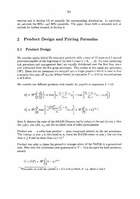
We consider equity-linked life insurance products with a term of 12 years and 5 annual premiums payable at the beginning of the first 5 years ( t = 0,. . . ,4). All costs (including risk premiums and management fees) are equally distributed over the first four years and subtracted from the five gross premiums. This results in five equal net premiums ( M ) . These five net premiums are swapped into a single premium which is used to buy a security that pays off A12 (as defined below) at expiration T = 12 if the insured person is still alive.
We consider two different products with benefit AT payable at expiration T = 12:
A+ = w & 6 (1 + max xl - ih,o 1=1 j=i I )
Here S j denotes the value of the DAX3O (German equity index) at the end of year J after the policy was sold, xlI2 are the secalled rates of index participation.
Product one - a collar-type product - pays compound interest on the net premiums. The interest in year j is calculated as XI times the DAX3O-return in year j but not less than i( 2 0 and no more than ih(> a,).'
Product two adds x2 times the geometric average-return of the DAX30 to a guaranteed sum. Note that this (minimum) sum guaranteed at T = 12 is the same for both products, namely
4
G = G(T) = f V x ( 1 $ i1)"-' i=O
'Principally, we could also consider ir < 0 in both products, cf., e.g., figures 1 and 2
Let At denote the value of the security at time t and let SWt denote the value of the above defined swap-contract at time t . Obviously mit has always a negative value to the insurance company and hence At + .SWt < 0 might occur (depending on the index volatility and the term structure of interest rate). Since the value of the policy has to be non negative, we define this value as & = max[At + SWt, 01. This is achieved by buying suitable options. These additional costs of course reduce the rate of index participation2.
To keep our notations as simple as possible, we assume throughout the paper that the policy is sold immediately after the date of the last balance sheet. In Germany, insurance companies have to provide such statements on a yearly basis, and we therefore only consider integer values for t in our further analysis.
2.2 Pricing Formulas
We will now state pricing formulas for the A!, t = 0, . . . ,11, k = 1 , 2 under the following assumptions:
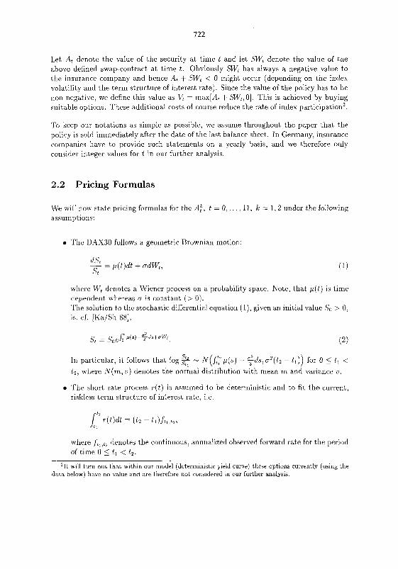
The DAX30 follows a, geometric Brownian motion:
where Wt denotes a Wiener process on a probability space. Note, that ~ ( t ) is time dependent whereas o is constant (> 0) 'l'be solution to the stochastic differential equation (1), given an initial value So > 0, is, ci. [Ka/Sh 881,
In particular, it follows that log 2 - N(J: p(s ) - $ d ~ , o2(tz - t l ) ) for 0 5 tl < t 2 , where N ( m , v) denotes the normal distribution with mean m and variance u.
The short rate process r ( t ) is assumed to be deterministic and to fit t he current, riskless term structure of interest rate, i.e.
where f t , denotes the continuous, annualized observed forward rate for the period of time 0 < t , < t2 .
21t will turn out that within our model (deterin~nistic yield curve) these options currently (using the da ta below) have no value and are therefore not considered in our further analysis.
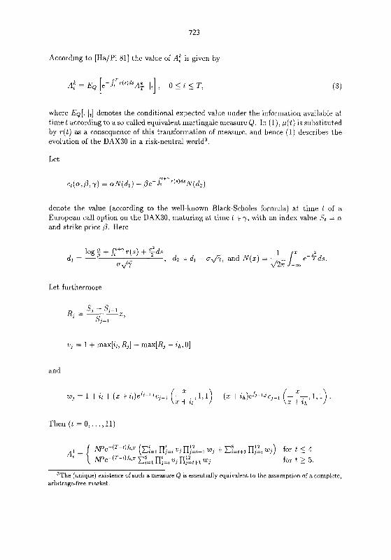
According to [Ha/Pl 811 the value of A,k is given by
where EQ( I t ] denotes the conditional expected value under the information available at t imet according to aso-called equivalent martingale measure Q. In (l), p( t ) is substituted by r ( t ) as a consequence of this transformation of measure, and hence ( I ) describes the evolution of the DAX30 in a risk-neutral world3.
Let
denote the value (according to the well-known Black-Scholes formula) at time t of a European call option on the DAXSO, maturing at time t + y, with an index value St = cu and strike price p. Here
log + htfr r (s ) + $ds l x 2 dl = , d2 = dl - u f i , and N ( r ) = --/ r - f ds .
0 8 Jz;; -m
Let furthermore
v, = 1 + max[il, R,] - max[R, - i h , 0 ]
and
Then (t = 0 , . . . ,11)
1 2 1 2 w e - ( T - t ) f t , ~ ( x i = , n : = , u, n,=,,, W , + E L + , n,,, w,) for t 5 4 = { w e - ( T - t ) f t , ~ ~5 t 1 2
I = ~ l-I,=! VJ rI,=t+l w, for t 2 5.
3The (unique) existence of such a measure Q is essentially equivalent to the assumption of a complete, arbitrage-free market
In particular,
A proof follows from Appendix 1 in [No 961.
For ~ r o d u c t 2 we get ( t = 0 , . . . ,11)
4
Af = C At,, + Gt, ,=o
where Gt = e-(T- t ) f t ,~G and At,, is given by
f o r t 5 i with
F o r t > i:
x A t , , - - e - ( ~ - ~ ) f t , ~ p { - e m + k ~ ( d l ) - x N ( d 2 ) } , St
with
In particular,
A proof for these formulas is given in Appendix A
2.3 The rate of index participation
Given the yield curve, the index volatility and ir , ih, the fair rate of index participation can now be calculated as a solution x > 0 of the implicit equation
a h - = ? W e - ~ b ' ( ~ ) " = prexnt value of net premiums, k = 1.2, 0 - r=O
if such a solution exists4.
For all of our empirical results we work with the term structure
and an index volatility of u = 12.98% as of January 22, 1997.
Varying il and ih , we get the following rates of index participation. In particular, both rates of index participation are quite sensitive with respect to the guaranteed interest rate i r .
Product 1:
-
41n case of product 1, there exists no solution if il 2 i; for some i; > 0. If, however, il < i;, there is an z;,(il) such that a unique solution exists if and only if ih > ii(il). Furthermore, zl -t co for ih \ i' h ( i I). For product 2 it is true, that there exists a unlque solution if and only if il < i; for some i; > 0.
Product 2:
il 11 0% '0 2% 1 4% xz 11 230.9% / 176.2% 1 110.8%
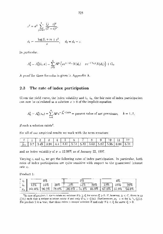
Figure 1 shows the rate of index participation for product 1 as a function of i l and ih, figure 2 shows the rate of index participation for product 2 as a function of ir.
Figure 1: xl = xl(i1, ih)
Figure 2: x 2 = xz ( i l )
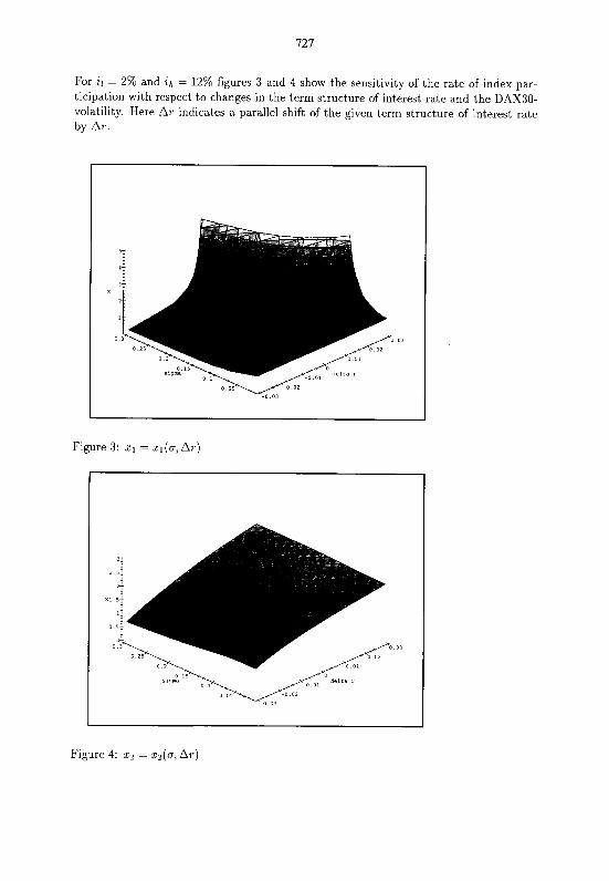
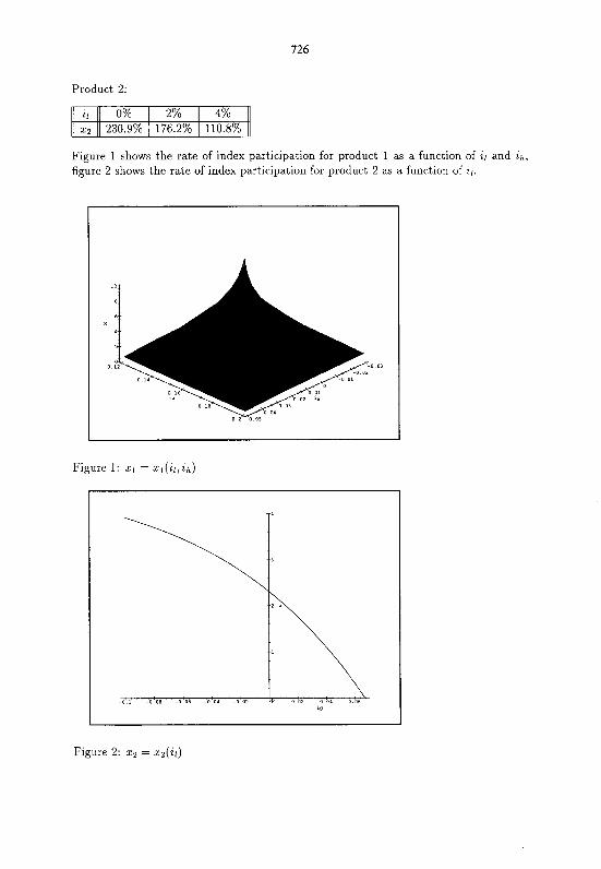
For ir = 2% and i h = 12% figures 3 and 4 show the sensitivity of the rate of index par- ticipation with respect to changes in the term structure of interest rate and the DAX3O- volatility. Here Ar indicates a parallel shift of the given term structure of interest rate by Ar.
r
I
Figure 3: X I = xl(u, Ar)
Figure 4: 22 = xz(o, Ar)
3 Additional Policy Reserves
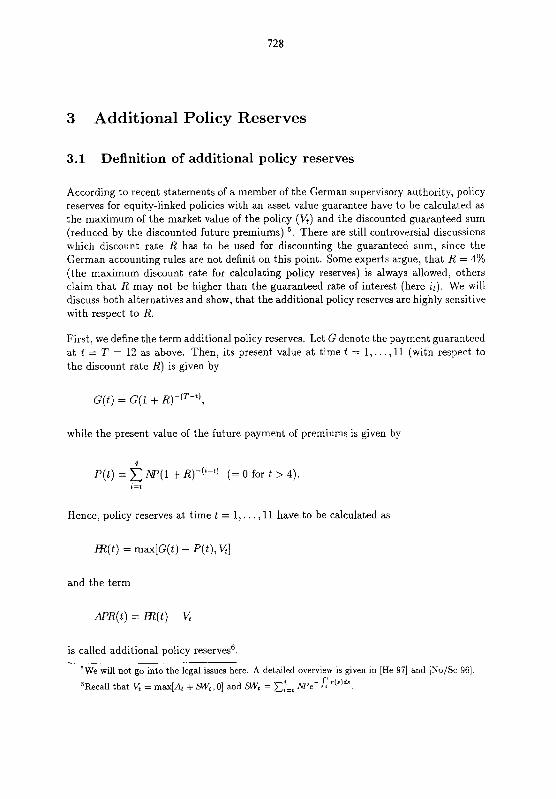
3.1 Definition of additional policy reserves
According to recent statements of a member of the German supervisory authority, policy reserves for equity-linked policies with an asset value guarantee have to be calculated as the maximum of the market value of the policy (V,) and the discounted guaranteed sum (reduced by the discounted future premiums) '. There are still controversial discussions which discount rate R has to be used for discounting the guaranteed sum, since the German accounting rules are not definit on this point. Some experts argue, that R = 4% (the maximum discount rate for calculating policy reserves) is always allowed, others claim that R may not be higher than the guaranteed rate of interest (here 2,). We will discuss both alternatives and show, that the additional policy reserves are highly sensitive with respect to R.
First, we define the term additional policy reserves. Let G denote the payment guaranteed at t = T = 12 as above. Then, its present value at time t = 1,. . . ,11 (with respect to the discount rate R) is given by
while the present value of the future payment of premiums is given by
4
P( t ) = W ( 1 + R)-("~) (= 0 for t > 4). r=t
Hence, policy reserves at time t = 1 , . . . ,11 have to be calculated as
and the term
is called additional policy reserves6.
'We will not go into the legal issues here. A detailed overview is given in [He 971 and [No/% 96)
'Recall that l/t = rnax[At + m,O] and SWt = Cf=, NPe-Lsr("d3.
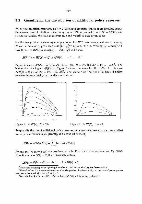
3.2 Quantifying the distribution of additional policy reserves
For further empirical results we fix ir = 2% for both products (which approximately equals the current rate of inflation in Germany), ih = 12% in product 1 and M> = 20000DEM (Deutsche Mark). We use the interest rate and volatility data given above.
For the first product, a meaningful upper bound for RPR(t) can easily be derived, defining A; as the value of At given that max [if, S'i:,-:-L z,] = il Vj 5 t . Writing V,* = max[A; + m,O] we set FR'(t) = max[G(t) - P(t ) , V,'] and hence
Figure 5 shows APR'(t) for if = 2%, it, = 12%, R = 2% and A r = 0%, . . . ,5%'. The higher Ar, the higher APR*(t). Figure 6 shows the same for R = 4%. In this case APR(t) = 0 Vt for AT = 076, 1%, 2%'. This shows that the risk of additional policy reserves depends highly on the discount rate R.
Figure 5: APR'(t), R = 2% Figure 6: APR'(t), R = 4%
To quantify the risk of additional policy reserves more precisely, we calculate the so called lower partial moments, cf. [Ha 911, and define (if existent)
for any real number a and any random variable X with distribution function Fx. With X = & and a = G(t) - P ( t ) we obviously obtain
'Note that according to our pricing formulas A: and hence APRg(t) are deterministic. 'Here the shift Ar is assumed to occur after the product has been sold, i.e. the rate of participation
has been calculated with Ar = 0 at t = 0. 'We note that for AT = -I%, -2% we have APR*(t) = 0 V t in figures 5 and 6
LPMl = E (APR(t)) = expected value of additional policy reserves at time t
which is the so called semi target variance. It is a more adeauate risk measure than "
the usual variance as it quantifies only the downside risk of missing the target. We furthermore define q,(t) to be the a-quantile of the distribution of APR(t).
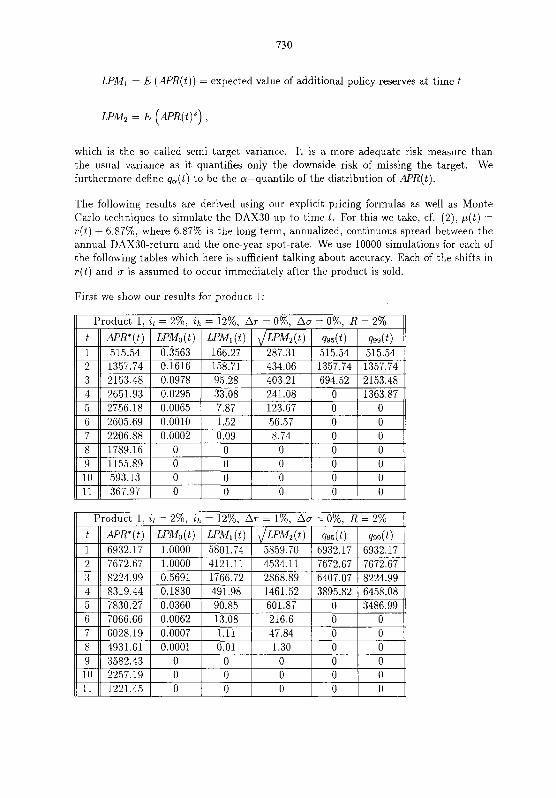
The following results are derived using our explicit pricing formulas as well as Monte Carlo techniques to simulate the DAX30 up to time t . For this we take, cf. (2), p(t) = ~ ( t ) + 6.87%, where 6.87% is the long-term, annualized, continuous spread between the annual DAX3O-return and the one-year spot-rate. We use 10000 simulations for each of the following tables which here is sufficient talking about accuracy. Each of the shifts in ~ ( t ) and a is assumed to occur immediately after the product is sold.
First we show our results for product 1:
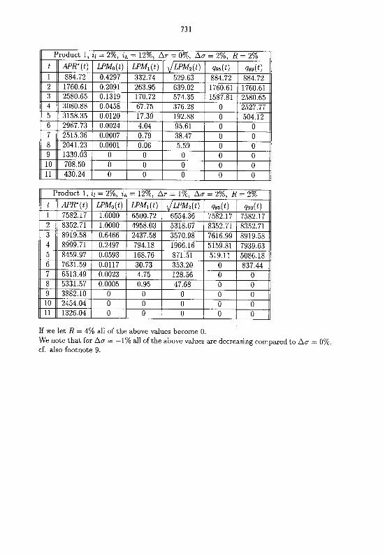
If we let R = 4% all of the above values become 0. We note that for Aa = -1% all of the above values are decreasing compared to Au = O%, cf. also footnote 9.
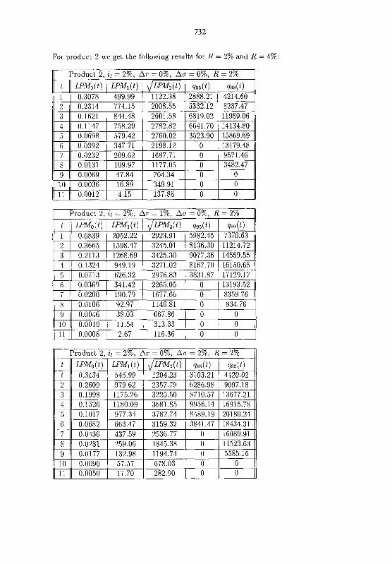
For product 2 we get the following results for R = 2% and R = 4%:

I Product 2, i l = 2%. Ar = 1%. Au = 2%. R = 2% 11
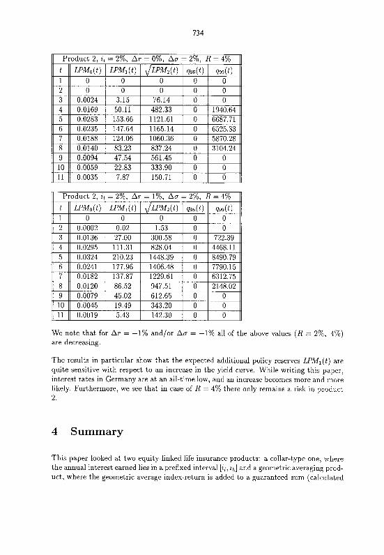
Product 2. ir = 2%. Ar = 0%. Aa = 2%. R = 4% I/
We note that for Ar = -1% and/or A o = -1% all of the above values (R = 2%, 4%) are decreasing.
Product 2 , ir = 2%, Ar = 1%, Aa = 2%, R = 4%
The results in particular show that the expected additional policy reserves LPMl(t) are quite sensitive with respect to an increase in the yield curve. While writing this paper, interest rates in Germany are at an all-time low, and an increase becomes more and more likely. Furthermore, we see that in case of R = 4% there only remains a risk in product 2.
t 1 2
4 Summary
This paper looked at two equity-linked life insurance products: a collar-type one, where the annual interest earned lies in a prefixed interval [il, ih] and a geometric averaging prod- uct, where the geometric average index-return is added to a guaranteed sum (calculated
LPMo(t) 0
0.0002
LPMI(~) 0
0.02
J L P M ~ ( ~ ) 0
1.53
~95( t ) 0 0
~ ( t ) 0 0
with il).
In the first part of the paper, we derived explicit pricing formulas for both products and showed, how to calculate the fair rate of index participation x, if the exogenous variables (yield curve, index volatility, i l , ih) are given. In both cases x depends heavily on ii, the minimum guaranteed interest rate.
Of course, the reader might ask, why we look at the geometric average instead of the arithmetic average. For the latter, no explicit pricing forrnulas are available, hence all calculations have to be done using extensive, time consuming Monte Carlo simulations. This is, in particular, unfavourable when calculating additional policy reserves at time t , as we do in Section 3. On the other hand it turns out, that using the data given in the paper, the rate of index participation in case of using an arithmetic average is almost identical to the one calculated for the geometric average product. Hence, it appears that the geometric average product can profitably be used in a control variate algorithm in order to speed up the Monte Carlo simulations considerably. So far, our discussion only focused on the product from an investment point of view.
In the second part of the paper, we calculated the additional policy reserves which are required, whenever the market value of the policy drops below the discounted sum guar- anteed at expiration on a date of the balance sheet. It turns out that the distribution of the additional policy reserves is quite sensitive with respect to changes in the interest rate level. Hence, it might be worthwhile using a stochastic interest-rate model - like the one-factor no-arbitrage model by Hull and White, cf. e.g. [Hu/Wh 941 - instead of a deterministic one.
A Proof of the Pricing Formula for the Geometric Average Product
We consider a security with the following payoff at maturity T = 12.
Let A,, denote the value of AT, at time t = 0 , . . . , 11, i . e A,,, = EQ [ r - f tTr( s )ds~ i , , I*]. In calculating this expected value, we follow an idea in [Tu/Wa 911.
Case 1: t = i
Given the information available at time t , we get
T - j + l SJ S, = log Si + C - log --- - N (m, s2),
~=;+l - SJ-l
with
m = log S, + C -
according to (2) (with p( t ) = r(t) , cf. our remark following (3))
Hence (with E - N(0, I)) ,
with
This is the distribution at time T of the value of a stock with current stock price (at time t ) S,e'J and volatility & in a risk-neutral world. Applying the formula of Black and Scholes, we get
with
Case 2: t < i
In this case we obviously get from (3) and (4)
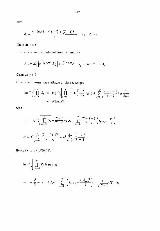
Case 3: t > i
Given the information available at time t , we get
T T - . l + l S, log -
3=t+l T - 2 S3-1
with
m = log T-2 \ l x + ~ l o g S t + -- T - j + l
j=i+l ,=t+1 T - i ( f w - ;)
Hence (with t - N ( 0 , I)),
This is the distribution at time T of the value of a stock with current stock price (at
time t ) ~ " + ~ - ( T - ' ) ~ ~ J and volatility + in a risk-neutral world. Applying thr formula of Black and Scholes, we get
with
Letting p, = 0 Vi we get the results of Section 2. Furthermore, if r ( t ) E const, our formulas for t 2 i coincide with a result in [Tu/Wa 911.
References
[Ha 911
[Ha/Pl 811
[He 971
[Hu/Wh 941
[Ka/Sh 881
[No 961
[No/Sc 961
Harlow, W.V. 1991: Asset-Allocation in a Downside-Rzsk Framework. Fi- nancial Analysts Journal, September/Oktober, 28-41.
Harrison, J.M. and Pliska, S.R. 1981: Martingales and stochastic integrals in the theory of continuous trading. Stochastic Processes and their Appli- cations 11, 215-260.
Herde, Armin 1997: Die Deckungsr~ckstellun~ bei der Aktienindexgebunde- nen Lebensversicherung. Versicherungswirtschaft 24, 1714.
Hull, John and White, Alan 1994: Numerical procedures for implementzng term structure models I: Single-Factor models. The Journal of Derivatives, Fall 1994, 7-16.
Karatzas, I. and Shreve, S.E. 1988: Brownian Motion and Stochastic Cal- culus. Springer, New York.
Nonnenmacher, Dirk Jens F. 1996: Indexgebundene Garantieprodukte. Working paper, University of Ulm.
Nonnenmacher, Dirk Jens F. and Schittenhelm, Frank Andreas 1996: Zusatzliche Deckungsruckstellungen: Das Aus fur die Aktienindexgebun- dene Lebensversicherung in Deutschland? To appear in Zeitschrift fiir die gesamte Versicherungswirtschaft.
Turnbull, Stuart M. and Wakeman, Lee Macdonald 1991: A Quick Al- gorithm for Pricing European Average Options. Journal of Financial and Quantitative Analysis, 26, 377-389.