Embed Size (px)
Citation preview
Equity Risk Premia and the VIX Term Structure
Travis L. Johnson∗
Stanford University
Graduate School of Business
Job Market Paper
November, 2011
Abstract
In many asset pricing models, the equity market’s expected return is a time-invariant
linear function of its conditional variance, which can be estimated from options markets.
However, I show that when the relation between conditional means and variances is
state-dependent, an observer requires the combined information in multiple variance
horizons to distinguish among the states and thereby reveal the equity risk premium.
Empirically, I show that while the VIX by itself has little predictive power for future
S&P 500 returns, the VIX term structure predicts next-quarter S&P 500 returns with
a 5.2% adjusted R2.
∗[email protected]. Thanks to Anat Admati, Mary Barth, Sebastian Infante, Arthur Korteweg,Kristoffer Laursen, Ian Martin, Stefan Nagel, Paul Pfleiderer, Monika Piazzesi, Ken Singleton, Eric So,and seminar participants at Stanford University.
1
Travis L. Johnson Equity Risk Premia and the VIX Term Structure November 2011
1. Introduction
There is mounting theoretical and empirical evidence of time variation in equity market
risk premia. These time variations are important both for economists studying asset pricing
and for market participants making portfolio allocation decisions. However, their use is
limited without an ex-ante observable measure of expected returns.
In many popular asset pricing models, risk premia can be inferred ex-ante as long as
the variance of future returns conditional on all available information is observable, for
example from options prices. In Campbell and Cochrane (1999) and Bansal and Yaron
(2004), conditional expected returns are an approximately linear, time-invariant, function
of conditional variance. These models therefore predict that the time-series of equity risk
premia and conditional equity variance are almost perfectly correlated, meaning that no
other variable predicts future equity returns incremental to conditional variance. Similarly,
recent models of variance risk premia and their connection with equity returns, in Bollerslev,
Tauchen, and Zhou (2009) and Drechsler and Yaron (2011), predict that expected returns are
a time-invariant linear function of return variance and the variance risk premia. Therefore,
these models also predict excess equity returns should be strongly predictable by measures
of conditional variance.
However, the data do not support these hypothesis. To quote Bollerslev, Tauchen, and
Zhou (2009), “a significant time-invariant expected return-volatility tradeoff type relationship
has largely proven elusive.” Conditional variance measures, whether constructed from option-
implied volatilities or time-series models, have economically and statistically weak predictive
power for future index returns.
In this paper, I argue that the expected return-conditional variance relation predicted by
theory is weak in the data because its nature changes every period. I show in a very general
model that expected returns are indeed related to conditional variance linearly, but that the
coefficients in this relation may change over time. In particular, the period-by-period shape
2
Travis L. Johnson Equity Risk Premia and the VIX Term Structure November 2011
of the variance-mean relation is determined by two economically meaningful quantities: the
regression coefficient of that period’s equity return on the stochastic discount factor (SDF
beta), and the variance of the part of returns orthogonal to the SDF (unpriced risk). The
aforementioned asset pricing models assume these two quantities are essentially constant.
However, when the market’s SDF beta and unpriced risk change over time, expected excess-
returns are no longer a time-invariant linear function of conditional variance.
Furthermore, I provide evidence that when risk premia are not easily inferred from con-
ditional variance, an observer who is unaware of the marginal investor’s preferences can
estimate equity risk premia using conditional variances at multiple horizons. In a stochastic
volatility model where the SDF beta and unpriced risk are mean-reverting state variables, I
show that the shape of the variance term structure allows an observer to decompose volatility
into its constituent factors by relying on differences in their persistence. As a result, risk
premia in the model are an affine function of the variance term structure.
I apply this technique to the S&P 500 index, which has liquid options markets for many
different strikes and times to expiration. Following the methodology used to calculate the
CBOE’s volatility index (VIX), I compute model-free implied volatility estimates at many
horizons, and show that the variance term structure can indeed dramatically improve index
return predictability. I find that the VIX term structure predicts future S&P 500 returns,
incrementally to any single VIX horizon, for holding periods from one month to one year. For
example, the combined term structure predicts next-quarter excess log returns on the S&P
500 with a 5.2% adjusted R2 and joint significance at the 1% level. The return predictability
is incremental to the “volatility risk premia” factor (Bollerslev, Tauchen, and Zhou (2009) and
Drechsler and Yaron (2011)), the aggregate dividend yield (e.g. Cochrane (2008) or Campbell
and Shiller (1988)), the net payout yield (Boudoukh et al. (2007)), and the Cochrane Piazzessi
factor from bond pricing (Cochrane and Piazzesi (2005)).
The majority of the incremental return predictability comes from the fourth principal
component of the VIX term structure, and not the first three (“level,” “slope,” and “curva-
3
Travis L. Johnson Equity Risk Premia and the VIX Term Structure November 2011
ture”) principal components. The factor has a “lightning bolt” shape, with loadings that slope
downwards over the first three VIX horizons, jump up sharply, and then slope down again
across the final three VIX horizons. It exhibits much less persistence than the VIX level,
mitigating concerns over the small-sample predictive bias discussed in Stambaugh (1999).
Finally, both the fourth principal component and risk premia fitted from the VIX term struc-
ture spike upwards around times of financial turmoil: the Asian financial crises (1997), the
LTCM collapse (1998), and in the later portion of the recent financial crises (2008-2009).
The exact linear combination of conditional variance horizons that reveals risk premia
in my model depends on the model’s parametrization. Therefore, the principal compo-
nent of the variance term structure that predicts future index returns also depends on the
parametrization. I show that a reasonable calibration of my model matches the regression
coefficients, as well as other relevant moments, observed in the data. Moreover, I show that
as long as the different state variables have different persistences, the combined information
in the VIX term structure provides an ex-ante measure of equity risk premia.
I discuss the paper’s relation to prior research in Section 2, detail the model of priced and
unpriced risks in the variance term structure in Section 3, show empirical results pertaining
to the S&P 500 in Section 4, and conclude in Section 5.
2. Relation to Prior Research
Two recent papers, Bollerslev, Tauchen, and Zhou (2009) and Drechsler and Yaron (2011),
study the relation between variance risk premia and equity risk premia. Empirically, both
show that the difference between end-of-month VIX2 and an estimate of statistical-measure
variance positively predicts future index returns. Bollerslev, Tauchen, and Zhou (2009) uses
past realized variance as a proxy for future statistical-measure variance, and Drechsler and
Yaron (2011) uses predicted future variance from a time-series model. In both papers, the
evidence for return predictability is statistically and economically strong from 1990-2007. I
show that the return predictability continues in the additional 2008-2010 years in my sample.
4
Travis L. Johnson Equity Risk Premia and the VIX Term Structure November 2011
Both papers postulate that this return predictability arises because the time-series of
the variance risk premia (VarQt (R) - VarPt (R)) and the equity risk premia are positively
correlated. Bollerslev, Tauchen, and Zhou (2009) derives this correlation in a discrete-time
model with time variation in both consumption volatility and the volatility of consumption
volatility. They show that the variance risk premium captures time variation in the volatility
of consumption volatility, which is also correlated with the time variation in risk premia.
Drechsler and Yaron (2011) derives the positive correlation between equity and variance
risk premia in broader setting that incorporates the long-run risk dynamics in Bansal and
Yaron (2004) and so can simultaneously match the magnitudes of the equity risk premia
and volatility risk premia we observe in the data, all while assuming a reasonable level of
risk aversion. In their model, the variance risk premia comes from a drift difference in the
consumption volatility process between Q and P, and from priced jump risk.
Both the Bollerslev, Tauchen, and Zhou (2009) and the Drechsler and Yaron (2011)
models predict no incremental role for the VIX term structure in capturing risk premia.
The reason is that both models have two priced factors: the variance risk premia and the
traditional risk-return relation (when conditional return volatility is high, expected returns
are high). The first can be captured empirically by using the variance differences described
above. The second is much simpler to implement empirically: a single VIX horizon should
reveal the current conditional variance. For this reason, both Bollerslev, Tauchen, and Zhou
(2009) and Drechsler and Yaron (2011) predict a much stronger VIX-return relation than the
one observed in the data, and no role for multiple VIX horizons. In my multifactor volatility
model, the nature of the variance-return relation varies across states, meaning there is a role
for multiple VIX horizons in extracting risk premia.
Mixon (2007) shows that the expectations hypothesis fails for the term structure of Black-
Scholes implied volatility, namely that the “forward” implied volatilities embedded in the
term structure are not one-for-one predictors of future realized “spot” implied volatilities. In
untabulated results, I replicate the failure of the expectations hypothesis for the new model-
5
Travis L. Johnson Equity Risk Premia and the VIX Term Structure November 2011
free VIX (as opposed to the old Black-Scholes based VXO used in Mixon (2007)) term
structure. Prior research also shows theoretically and empirically that VIX term structure
can be used to price VIX futures and options (e.g. Sepp (2008), and Zhu and Zhang (2007)).
Duan and Yeh (2011) fits a fairly general single-factor stochastic volatility model to the
observed S&P 500 index return and VIX term structure processes using a particle-filter based
estimation. By contrast, I use a multifactor volatility model to study the relation between
the VIX term structure and equity risk premium (rather than contemporaneous returns) and
calibrate the model to match empirical moments rather than structurally estimating it.
To my knowledge, the only multifactor model of index volatility is in Christoffersen,
Heston, and Jacobs (2009), which extends the Heston (1993) model by allowing the volatility
process be the sum of two square-root processes. The two-factor volatility model is able to
capture the relative independence of the level and slope of the “smirk” observed in implied
volatilities and therefore dramatically improve the upon the option pricing compared to
Heston (1993). I augment their analysis by adding a time-varying SDF beta, looking at
different times-to-expiration rather than different strike prices, and examining the economic
relation between variance and expected returns.
My central argument, that the VIX term structure allows an observer to distinguish
among components of the VIX that have different prices and persistences, has an analogue
in the bond return predictability literature. If the short-rate process is composed of multiple
factors with different pricing and persistences, like the volatility process in my model, the
shape of the yield curve could be used to distinguish between different short-rate factors
and thereby better estimate bond risk premia. The bond risk premia literature (Dai and
Singleton (2002), Cochrane and Piazzesi (2005), Cochrane and Piazzesi (2008), and the
references therein) provides theoretical and empirical evidence that the shape yield of the
curve reveals bond risk premia when there are multiple factors.
There is a fundamental distinction, however, between the VIX term structure predicting
equity index returns and the bond term structure predicting excess bond returns. In bond
6
Travis L. Johnson Equity Risk Premia and the VIX Term Structure November 2011
markets, the predicted returns are for the same asset whose yields determine the term struc-
ture. In this paper, I use the term structure of option-implied variance to predict the returns
of the underlying asset, relying on the economic connection between conditional variance and
equity risk premia. The equivalent analysis for the treasury yield curve would examine the
relation between bond risk premia and the term structure of bond return variance implied
by bond options.
3. Model
The driving intuition in my model is that if the relation between conditional variance
and risk premia is state-dependent, examining market expectations of volatility at multiple
horizons allows an otherwise uninformed observer to distinguish between states and better
estimate risk premia.
I begin by illustrating the relation between variance and returns with two minimal as-
sumptions: no arbitrage, and the existence of a conditionally riskless asset. Together these
assumptions imply that there exists a stochastic discount factor (SDF) M̃t+1 that prices any
traded asset i with gross return R̃i,t+1 as follows:
Et(R̃i,t+1)−Rf,t = −covt(R̃i,t+1, M̃t+1)Rf,t (1)
where Rf,t is the gross risk-free rate at time t. I drop the subscript i hereafter for brevity.
Now define αt, βt, and ε̃t+1 so that:
R̃t+1 = αt − βtM̃t+1 + ε̃t+1 (2)
βt =−covt(R̃t+1, M̃t+1)
vart(M̃t+1)(3)
covt(M̃t+1, ε̃t+1) = 0 (4)
With this sign convention, assets with a positive βt have a negative correlation with the SDF
7
Travis L. Johnson Equity Risk Premia and the VIX Term Structure November 2011
and are therefore subject to systematic risk. Note that αt−βtM̃t+1 is the projection of R̃t+1
onto M̃t+1, and that equation (2) is not a time-series regression because the coefficients αt
and βt may be different in each period.
Combining equations (1) and (3), and computing the variance of R̃t+1 from equation (2)
gives:
Et(R̃i,t+1)−Rf,t = βtvart(M̃t+1)Rf,t (5)
vart(R̃t+1) = β2t vart(M̃t+1) + vart(ε̃t+1) (6)
The reason for manipulating the basic pricing equation into equations (5) and (6) is that
these equations express both the conditional mean and variance of future returns as simple
functions of three economically meaningful variables. The first, SDF variance vart(m̃t+1),
is an economy-wide variable, while the second, SDF beta βt, is asset-specific. Both are
reflected in risk premia (equation (5)) as well as return variance (equation (6)). The final
variable is the residual variance vart(ε̃t+1), which is also asset-specific and only impacts the
return variance but not the mean of returns, and so I call it unpriced risk.
To help interpret the SDF variance, SDF beta, and unpriced risk in what follows, I
discuss the meaning of each in the context the asset pricing literature. The conditional SDF
variance vart(M̃t+1) is the variance of investor’s marginal utility of consumption in the next
period. Changes in the volatility of marginal utility could be due to changes in the volatility
of consumption growth (as in Bansal and Yaron (2004)), or to changes in the risk aversion of
the marginal investor (as in Campbell and Cochrane (1999)). In this framework, both effects
are absorbed into the SDF variance and impact expected returns and conditional variances
for all traded assets.
The best analogies for the SDF beta βt and the unpriced variance vart(ε̃t+1) come from
the CAPM. The asset-specific SDF beta βt serves the same role as the asset-specific “market
beta” in the a period-by-period CAPM: it measures the exposure to priced risk for a specific
8
Travis L. Johnson Equity Risk Premia and the VIX Term Structure November 2011
asset. Similarly, what I call unpriced risk is analogous to “idiosyncratic volatility” in the
CAPM. Both are orthogonal to what investor’s care about: market returns in the CAPM
and the more general SDF M̃t in this framework. If the CAPM holds period-by-period,
the market portfolio is perfectly correlated with the SDF, implying that it has no unpriced
risk. Other traded assets and portfolios, however, could have time variation in both βt and
vart(ε̃t+1).
Theorem 1 illustrates the general relation between conditional variance and the condi-
tional risk premium.
Theorem 1. Assuming no arbitrage, for any risky asset with returns R̃t+1 and any SDF
M̃t+1 that prices R̃t+1, we have:
Et(R̃t+1)−Rf,t = A0,t + A1,tvart(R̃t+1) (7)
where A0,t = − vart(ε̃t+1))Rf,tβt
, A1,t =Rf,tβt
, and the other variables are defined above.
Proof. Manipulating equations (5) and (6) yields:
Et(R̃t+1)−Rf,t = (vart(R̃t+1)− vart(ε̃t+1))1
βtRf,t (8)
Equation (7) abbreviates this using the A0,t and A1,t notation.
Note that Theorem 1 holds regardless of the time horizon, investor preferences, and for
all types of assets. The only necessary assumptions are that there is a riskless asset, and that
there is no arbitrage. In fact, equation (7) simplifies to the original pricing equation (1) with
enough substitution. However, equation (7) is a useful representation because theoretical
models often provide some structure for A0,t and A1,t, from which we can use equation
(7) to find ex-ante observable expected return estimates using ex-ante conditional variance
estimates. The remainder of this section discusses different specifications for A0,t and A1,t.
Theorem 1 examines a special case where both the SDF beta and unpriced risk are
9
Travis L. Johnson Equity Risk Premia and the VIX Term Structure November 2011
constant across time. This occurs when, while risk premia may be changing each period
through changes in the SDF variance, the relation between M̃t+1 and R̃t+1 has the same
slope and residual variance in each period. I show that this implies all time variation in risk
premia can be captured by a time-invariant linear function of conditional variance. Moreover,
I show the converse: if risk premia for any asset are a linear function of conditional variance,
it implies that the asset has constant SDF beta and constant unpriced risk.
Corollary 1. Assuming the risk-free rate is fixed at Rf,t = Rf , and there is no arbitrage,
the following two statements are equivalent:
1. Unpriced risk is fixed at vart(ε̃t+1)) = σ2ε and the SDF beta is fixed at βt = β.
2. There exist constants A0 and A1 such that Et(R̃t+1)−Rf = A0+A1vart(R̃t+1) in every
period t.
Proof. Suppose vart(ε̃t+1)) = σ2ε and βt = β. Plugging these values into A0,t and At,1 yields
constant coefficients, meaning Theorem 1 implies Et(R̃t+1) − Rf,t = A0 + A1vart(R̃t+1) in
each period where A0 = −σ2εRfβ
A1 =Rfβ.
Now suppose we have constants A0 and A1 such that Et(R̃t+1)−Rf,t = A0+A1vart(R̃t+1)
in every period. This implies that unpriced risk and SDF beta are constant over time, because
if they were not, equation (7) would imply time-varying coefficients in the relation between
risk premia and variance, a contradiction.
The statements in Theorem (1) may seem quite restrictive, but they are met or nearly
met in many modern asset pricing models. Both Campbell and Cochrane (1999) and Bansal
and Yaron (2004), for example, predict that nearly all of the time-variation in equity risk
premia is captured by a linear function of conditional return variance (see Appendix A
for details). The reason is that both assume equity markets provide a claim to dividends
whose growth has constant correlation with consumption growth. This means that both the
unpriced risk vart(ε̃t+1), and the SDF beta βt, are nearly constant across different states of
the model. As a result, both models imply that a time invariant linear function conditional
10
Travis L. Johnson Equity Risk Premia and the VIX Term Structure November 2011
variance captures nearly all the variation in risk premia, meaning that conditional variance
should predict future market returns and that nothing else should have significant predictive
power incremental to conditional variance. A similar result applies in the models of variance
risk premia in Bollerslev, Tauchen, and Zhou (2009) and Drechsler and Yaron (2011); both
models predict a strong linear relation between conditional variance and future returns in
addition to the relation between variance risk premia and future returns.
Empirically, as detailed in Section 4, the relation between realized returns and conditional
variance is weak. Moreover, there appears to be several other other variables that capture
risk premia better than conditional variances, namely the variance risk premia, the price-
dividend ratio, and the variance term structure. These results suggest that the market’s
SDF beta and unpriced variance change over time. In the next subsection, I impose some
structure of the state variables that govern the variance-return relation, and show how the
variance term structure can be combined to provide an observable measure of ex-ante risk
premia when conditional variance alone is not enough.
3.1. A three-factor model of variance and risk premia
I present a dynamic, discrete time, discrete state model of the relation between risk
premia and the variance term structure. I focus here on the simplest possible framework
that conveys my results. A more realistic continuous time, continuous state, version of the
model in the Appendix C produces qualitatively identical conclusions.
In each period, the stochastic discount factor M̃t+1 and the simple equity return R̃t+1
each take one of two values:
M̃t+1 =
1Rf
+ σM,t w.p. 12
1Rf− σM,t w.p. 1
2
R̃t+1 =
µt + σR,t w.p. 12
µt − σR,t w.p. 12
where Rf is the risk-free rate, constant over time to focus my results on the term structure
of variance and not interest rates, σM,t is the standard deviation of M̃t+1, µt is the expected
equity return, and σR,t is the standard deviation of returns. The SDF and return innovations
11
Travis L. Johnson Equity Risk Premia and the VIX Term Structure November 2011
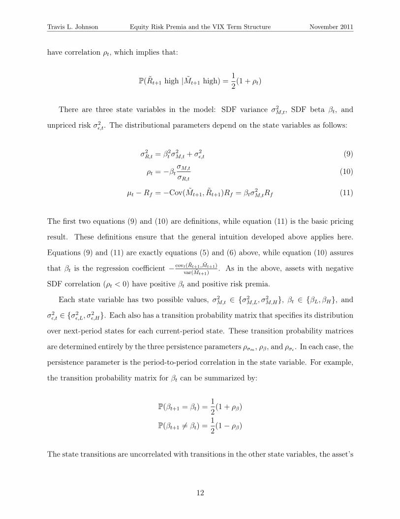
have correlation ρt, which implies that:
P(R̃t+1 high |M̃t+1 high) =1
2(1 + ρt)
There are three state variables in the model: SDF variance σ2M,t, SDF beta βt, and
unpriced risk σ2ε,t. The distributional parameters depend on the state variables as follows:
σ2R,t = β2
t σ2M,t + σ2
ε,t (9)
ρt = −βtσM,t
σR,t(10)
µt −Rf = −Cov(M̃t+1, R̃t+1)Rf = βtσ2M,tRf (11)
The first two equations (9) and (10) are definitions, while equation (11) is the basic pricing
result. These definitions ensure that the general intuition developed above applies here.
Equations (9) and (11) are exactly equations (5) and (6) above, while equation (10) assures
that βt is the regression coefficient − covt(R̃t+1,M̃t+1)
var(M̃t+1). As in the above, assets with negative
SDF correlation (ρt < 0) have positive βt and positive risk premia.
Each state variable has two possible values, σ2M,t ∈ {σ2
M,L, σ2M,H}, βt ∈ {βL, βH}, and
σ2ε,t ∈ {σ2
ε,L, σ2ε,H}. Each also has a transition probability matrix that specifies its distribution
over next-period states for each current-period state. These transition probability matrices
are determined entirely by the three persistence parameters ρσm , ρβ, and ρσε . In each case, the
persistence parameter is the period-to-period correlation in the state variable. For example,
the transition probability matrix for βt can be summarized by:
P(βt+1 = βt) =1
2(1 + ρβ)
P(βt+1 6= βt) =1
2(1− ρβ)
The state transitions are uncorrelated with transitions in the other state variables, the asset’s
12
Travis L. Johnson Equity Risk Premia and the VIX Term Structure November 2011
return, and the SDF. Such correlations exist in the data, as evidenced by the fact that return
variance tends to go up when markets go down (the so-called “leverage effect”). A version
of this model with state innovations correlated with the SDF generates the leverage effect,
but adds complexity without changing the relation between variance term structure and risk
premia.
3.1.1 Observing risk premia in the model
While the marginal investor knows their preferences and the distribution of asset values,
and can therefore compute the three volatility states σ2M,t, βt, and σ2
ε,t, I study the problem of
an outside observer hoping to infer the state using traded asset prices. For such an observer,
the equity price reveals nothing about the volatility state. Observing past returns could
reveal the past volatility of returns σ2R,t−1 but neither the state variables that compose σ2
R,t−1
nor the current volatility of returns σ2R,t.
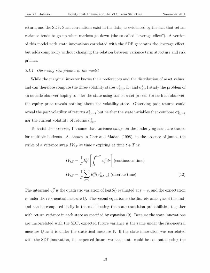
To assist the observer, I assume that variance swaps on the underlying asset are traded
for multiple horizons. As shown in Carr and Madan (1998), in the absence of jumps the
strike of a variance swap IVt,T at time t expiring at time t+ T is:
IVt,T =1
TEQt
[∫ t+T
t
vRs ds
](continuous time)
IVt,T =1
T
T−1∑s=0
EQt (σ
2R,t+s) (discrete time) (12)
The integrand vRs is the quadratic variation of log(St) evaluated at t = s, and the expectation
is under the risk-neutral measure Q. The second equation is the discrete analogue of the first,
and can be computed easily in the model using the state transition probabilities, together
with return variance in each state as specified by equation (9). Because the state innovations
are uncorrelated with the SDF, expected future variance is the same under the risk-neutral
measure Q as it is under the statistical measure P. If the state innovation was correlated
with the SDF innovation, the expected future variance state could be computed using the
13
Travis L. Johnson Equity Risk Premia and the VIX Term Structure November 2011
state transition probabilities under Q.
As discussed in more detail in Section 4, without data on variance swap pricing an
observer can still compute IVt,T from the time t price of call and put options expiring at
time t+T at enough different strike prices. The square of the CBOE’s VIX index is exactly
such a computation, as are the model-free implied variance estimates discussed in Britten-
Jones and Neuberger (2000), Jiang and Tian (2005), and elsewhere.
I show that the combined information in IVt,T at many different horizons T can completely
reveal the volatility state (σ2M,t, βt, σ2
ε,t), and therefore reveal any time variation in the equity
risk premia. Intuitively, the reason is that when the different components of volatility have
different persistences, many different volatility states could produce the same IVt,T for a
single T , but each volatility state produces a unique shape of the IVt,T term structure. This
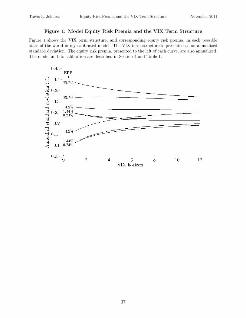
intuition can be seen clearly in Figure 1, which shows the VIX term structure in each of
the eight different states of the world1, as well as the annualized equity premia. Due to
the array of possible SDF betas and unpriced risk, the equity risk premia is a non-linear,
non-monotonic, function of conditional variance for any single horizon. However, each state
of the world is easily identifiable from the shape of the term structure.
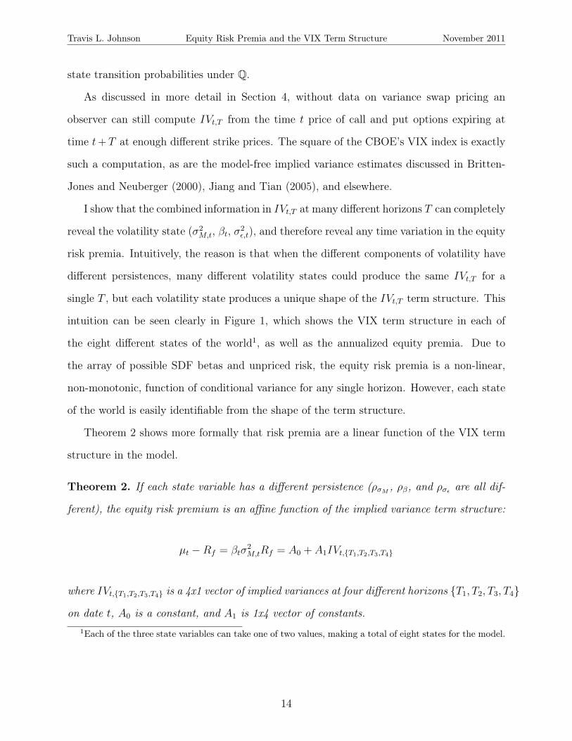
Theorem 2 shows more formally that risk premia are a linear function of the VIX term
structure in the model.
Theorem 2. If each state variable has a different persistence (ρσM , ρβ, and ρσε are all dif-
ferent), the equity risk premium is an affine function of the implied variance term structure:
µt −Rf = βtσ2M,tRf = A0 + A1IVt,{T1,T2,T3,T4}
where IVt,{T1,T2,T3,T4} is a 4x1 vector of implied variances at four different horizons {T1, T2, T3, T4}
on date t, A0 is a constant, and A1 is 1x4 vector of constants.1Each of the three state variables can take one of two values, making a total of eight states for the model.
14
Travis L. Johnson Equity Risk Premia and the VIX Term Structure November 2011
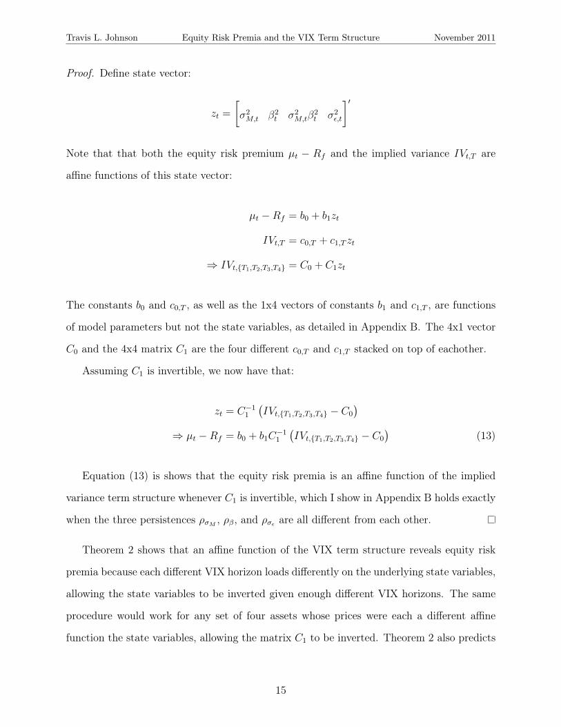
Proof. Define state vector:
zt =
[σ2M,t β2
t σ2M,tβ
2t σ2
ε,t
]′
Note that that both the equity risk premium µt − Rf and the implied variance IVt,T are
affine functions of this state vector:
µt −Rf = b0 + b1zt
IVt,T = c0,T + c1,T zt
⇒ IVt,{T1,T2,T3,T4} = C0 + C1zt
The constants b0 and c0,T , as well as the 1x4 vectors of constants b1 and c1,T , are functions
of model parameters but not the state variables, as detailed in Appendix B. The 4x1 vector
C0 and the 4x4 matrix C1 are the four different c0,T and c1,T stacked on top of eachother.
Assuming C1 is invertible, we now have that:
zt = C−11
(IVt,{T1,T2,T3,T4} − C0
)⇒ µt −Rf = b0 + b1C
−11
(IVt,{T1,T2,T3,T4} − C0
)(13)
Equation (13) is shows that the equity risk premia is an affine function of the implied
variance term structure whenever C1 is invertible, which I show in Appendix B holds exactly
when the three persistences ρσM , ρβ, and ρσε are all different from each other.
Theorem 2 shows that an affine function of the VIX term structure reveals equity risk
premia because each different VIX horizon loads differently on the underlying state variables,
allowing the state variables to be inverted given enough different VIX horizons. The same
procedure would work for any set of four assets whose prices were each a different affine
function the state variables, allowing the matrix C1 to be inverted. Theorem 2 also predicts
15
Travis L. Johnson Equity Risk Premia and the VIX Term Structure November 2011
that all variation in expected returns are captured by an affine function of the VIX term
structure, meaning that the VIX term structure (and nothing else) should predict future
equity returns in a linear regression.
3.1.2 Calibrated Model
I present sample moments for a specific calibration of my model in order to illustrate
that the regression coefficients relating the VIX term structure to future index returns, as
described in Section 4, can arise in my relatively simple model. I calibrate the model to
data on the S&P 500 by matching the moments listed in Table 1. The unit of time is one
month, and I use the VIX term structure as described in Section 4 as a measure of the risk-
neutral expected return variation. I show that the calibrated model is capable of generating
weak return predictability for a single variance horizon and strong return predictability for
multiple variance horizons, with coefficients closely matching those in the data.
The first four moments in Table 1 are the unconditional mean of the one-month VIX and
the standard deviations of the VIX at three different horizons. I calculate the unconditional
mean VIX level under the statistical measure to match the data, but the model VIX itself is a
risk-neutral expectation of future diffusion, as described above. The longer-horizon VIX are
less volatile in both the model and the data because volatility mean reverts, meaning that the
short-horizon VIX is normally farther from the long-run mean than the long-horizon VIX.
The calibrated model matches these four moments fairly well, although the longer horizon
VIX are more volatile in the data than the model.
The next two moments are the mean and variance of monthly excess returns. In the
model, expected returns and statistical variance are given by equations (11) and (9), respec-
tively. The calibrated model matches the unconditional risk premium quite closely. However,
returns in the calibrated model are too volatile under the statistical measure. In the model,
there is no difference between statistical and risk-neutral volatility, and so it cannot repli-
cate the dramatic difference between average VIX21 and realized return variance (variance
risk premia) observed in the data. If the model were extended to allow correlation between
16
Travis L. Johnson Equity Risk Premia and the VIX Term Structure November 2011
the SDF and innovations in the volatility states, there would be a positive variance risk
premia.
The next moment is the correlation between the one-month VIX and the one-month VIX
one month ago, which is is determined in the model by the combined persistence of the three
different volatility measures. The calibrated model produces a 0.758 correlation, while the
correlation in the data is 0.805.
Moments labelled (8)-(12) in Table 1 are regression coefficients from a single regression
of the simple excess return Rt+1−Rf,t on a constant and VIX1,t; and a multiple regression of
Rt+1−Rf,t on a constant, VIX21,t, VIX2
3,t, VIX26,t, and VIX2
12,t. The calibrated model matches
the weakly positive single regression slope coefficient, as well as the “lightning bolt” shape
of the multiple regression coefficients2. I match coefficients with only four of the six VIX
horizons because, as shown in Theorem 2, any four VIX horizons completely reveals the risk
premia in the model, meaning a regression with more than four horizons is not identified.
Table 1 also presents the model parameters used in calibration. In order to match the
remarkable volatility in the VIX index observed in my 1996-2010 sample, the spread between
high and low parameter values is quite large. For example, the SDF variance is 0.06 in its
high state and 0.01 in its low state. The persistence parameters are primarily responsible
for the regression coefficients in the multi-VIX regression. A calibration with persistences
0.95 for SDF beta, 0.85 for SDF variance, and 0.55 for unpriced risk produces approximately
the regression coefficients observed in the data. A different persistence combination would
produce different regression coefficients, but as long as the state variables each have different
persistences, the VIX term structure provides incremental return predictability beyond a
single VIX horizon.2The coefficients used in this calibration do not exactly match those in Table 3 because they pertain to
regressions with simple returns, rather than log returns, on the left-hand side.
17
Travis L. Johnson Equity Risk Premia and the VIX Term Structure November 2011
4. Empirical Results
In order to study the relation between conditional variances and risk premia, I need an
empirical measure of conditional variance. I use an option-based measure, rather than a
forecast from a time-series volatility model, because options markets are able to incorporate
all public information about future variances. Time-series volatility models, on the other
hand, can only incorporate conditioning variables that are both observable and incorporated
into the model, making them inherently backward-looking. The drawback of the option-
implied variance measure is that it produces risk-neutral rather than statistical variances,
an issue I return to later.
I compute the VIX term structure by replicating the CBOE’s VIX calculation3, but with
longer horizons than 30 days. The VIX calculation is based on the model-free implied volatil-
ity measure originating from Breeden and Litzenberger (1978). Assuming the availability of
options at every strike price, the VIX is defined by:
VIX2 ≡ 2erT
T
{∫ Ft
0
1
K2putT (K)dK +
∫ ∞Ft
1
K2callT (K)dK
}(14)
where putT (K) and callT (K) are the prices at time 0 of puts and calls expiring at time T
with strike price K. As shown in Neuberger (1994) and Carr and Madan (1998), if the S&P
500 follows a diffusion process dSt = rStdt + σtStdZt under the risk-neutral measure, VIX2
equals the risk-neutral expectation of average future instantaneous variance EQ[∫ T
0σ2t dt].
An alternate option-implied variance measure is the SVIX from Martin (2011), which is
defined by:
SVIX2 ≡ 2erT
T
{∫ Ft
0
1
S20
putT (K)dK +
∫ ∞Ft
1
S20
callT (K)dK
}(15)
Equation (15) uses the same notation at equation (14) with the addition of S0, the price3See www.cboe.com/micro/vix/vixwhite.pdf for more details.
18
Travis L. Johnson Equity Risk Premia and the VIX Term Structure November 2011
of the underlying at time 0. Martin (2011) shows that the SVIX measures the risk-neutral
variance of simple returns from time 0 to time T, and unlike the VIX its interpretation is
robust to the presence of jumps. The SVIX2 and VIX2 turn out to be very highly correlated
in the data, with the VIX2 exceeding the SVIX2 significantly only during periods of crisis like
the fall of 2008. My empirical results employ the widely-followed VIX but are qualitatively
identical when using SVIX.
The standard approach to estimating the VIX equation (14) empirically, used by the
CBOE to compute the VIX, discretizes the integral at the available strike prices and truncates
it at the smallest and largest available strike prices. Jiang and Tian (2005) discusses each as
a potential source for estimation error and, using simulated data, conclude that the number
of strikes available for S&P 500 index options is sufficient to compute the one-month VIX.
However, at longer horizons, options are less liquid and the range of plausible index values is
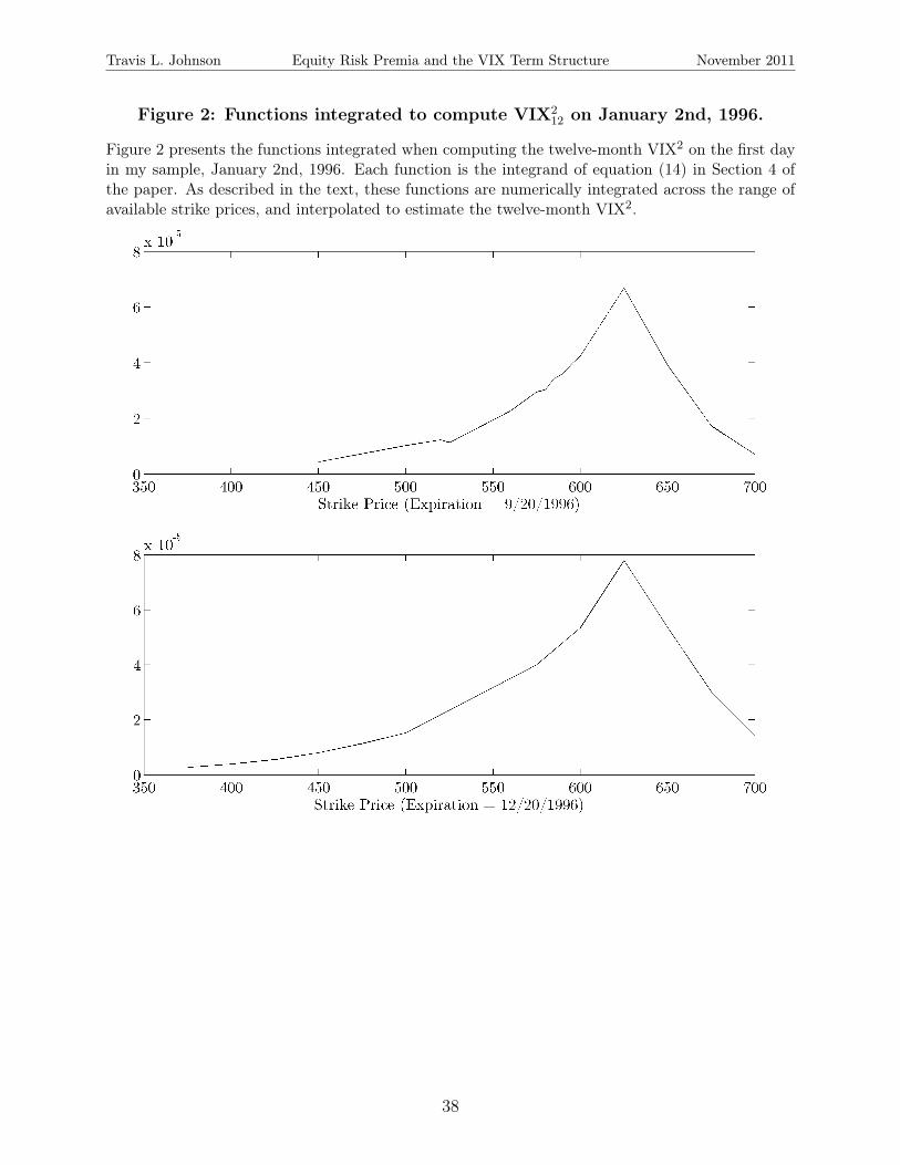
larger. For that reason, Figure 2 presents the numeric integrals used to compute the twelve-
month VIX on the first day of my sample, likely to be the worst day/horizon pair in my
analysis. The twelve-month VIX is the linear interpolation of the VIX estimates on the two
nearest expiration dates in the data, computed as the area under the two curves in Figure
2. While there is clearly some truncation error, especially for the range of strikes above
700, it looks to be only a small percentage of the total area under each curve. Critically,
since equation (14) relies heavily on out-of-the-money put options with low K and high 1K2 ,
liquidity in options markets tilts heavily towards exactly these options.
The results in Bollerslev, Tauchen, and Zhou (2009) and Drechsler and Yaron (2011)
indicate that past realized volatility, controlling for the forward-looking VIX, negatively
predicts future index returns. To examine the incremental predictive power of the VIX term
structure, I therefore need to control for realized volatility in my regressions. For a measure
of realized volatility, I follow Drechsler and Yaron (2011) and use intraday S&P 500 futures
data provided by tickdata.com. More specifically, I compute a time series of five-minute
19
Travis L. Johnson Equity Risk Premia and the VIX Term Structure November 2011
returns for S&P 500 futures and estimate the variation of log returns from t− 1 to t using:
R̂V =n∑j=1
[log(Rt−1+ j
n
)]2
Intraday data at five-minute intervals has the advantage of more accurately estimating return
variation than coarser daily data, but has the disadvantage that it requires accurate intraday
prices. As discussed in Drechsler and Yaron (2011), the S&P 500 index level can often have
stale prices in intraday data because it is the aggregation of 500 different prices, and not
traded directly. S&P 500 futures, by contrast, are a single actively-traded asset, making
stale prices much less likely.
Using closing option quotes for S&P 500 index options and risk-free rates available from
1996 through 2010 via OptionMetrics, I compute the VIX term structure and a rolling
estimate of past one-month return variation at the close of markets each day. Occasionally
in my sample period, there were option expiries on the last trading day of the quarter in
addition to the normal third Saturday of every month. I remove these observations because
they generally did not have nearly the volume or range of strike prices offered by the normal
expiration dates. I also remove a handful day/expiration date pairs which appear to have
missing data in OptionMetrics, as well as a few individual option prices that are clearly data
errors.
Table 2 presents some descriptive statistics for the VIX term structure, including VIX2T
for T = 1, 2, 3, 6, 9, and 12months. These horizons were chosen to represent the approximate
times-to-expiration available at any given time for index options. The first thing to note is
that, on the median day, the term structure is upwards sloping from T = 1 to T = 6 and
then about flat out until T = 12. There is, however, some variability in the shape of the
term structure, for example the interquartile range of VIX26
VIX21is 0.95 to 1.31. Finally, the entire
VIX term structure tends to be much higher than past realized volatility, though in some
rare cases this relation can reverse.
20
Travis L. Johnson Equity Risk Premia and the VIX Term Structure November 2011
Figure 3 plots the evolution of the term structure over my 1996-2010 sample. The primary
thing to notice is that the term structure is downward sloping when VIX21 is particularly high,
and upward sloping when VIX21 is particularly low. This suggests that investors assume some
mean reversion in volatility will bring it “towards normal” over the next year. Another salient
feature of the VIX term structure visible in Figure 3 is that while the different VIX horizons
are strongly correlated with one another, there are changes in the exact shape of the term
structure beyond its level and slope.
Table 3 illustrates the predictive power of the VIX term structure for future returns.
The dependent variable is future S&P 500 index returns, inclusive of dividends, starting at
the close of markets one day after the observation of the VIX term structure. The one day
gap is important because options markets close 15 minutes later than equity markets. The
independent variables are the option-implied variances at different horizons, as measured by
V IX2T . These are scaled to be monthly variances in order to match the time period used for
the model in Section 3.
Panel A shows that, by itself, the one-month VIX has no predictive power for future one-
and three-month returns, statistically insignificant power for future six-month returns, and
some predictive power for one-year returns. Adding the full VIX term structure (VIX22 ...
VIX212) dramatically increases the return predictability, adding 1.99%, 5.16%, 6.60%, and
3.73% in incremental R2 for the one-, three-, six-, and twelve-month horizons, respectively.
I reject the null hypothesis that the five longer horizon VIX all have coefficients equal to
zero with p values 0.1%, 0.1%, and 0.4% for the three-, six-, and twelve-month horizons. I
cannot reject the null for next-month returns. The intermediate rows, which only include
VIX21, VIX2
6, and VIX212, demonstrate that the addition of two longer-horizon VIX provides
much, but not all, of the incremental predictive power gained by the VIX term structure.
Panel B repeats the analysis in Panel A but with past realized variance RV (defined
above) as an additional regressor. As demonstrated in Bollerslev, Tauchen, and Zhou (2009)
and Drechsler and Yaron (2011), the difference between VIX21 and RV predicts future index
21
Travis L. Johnson Equity Risk Premia and the VIX Term Structure November 2011
returns quite well. However, at all horizons the predictive power of the VIX term structure
is incremental to the predictability afforded by VIX21 and RV. I can reject the null hypothesis
that the coefficients on VIX2T are all zero for T ≥ 2 after controlling for VIX2
1 and RV with
p-values of 0.3%, 0.1%, and 0.3% for the three-, six-, and twelve-month horizons. As in Panel
A, I cannot reject the null for one-month returns. At all horizons there is also a substantial
increase in R2 upon the addition of the VIX term structure.
Finally, Panel C shows that the VIX term structure predicts returns incrementally to
three predictors established in prior research. The first is the dividend yield, measured as
the log of the prior year’s total market-wide dividends scaled by the current total market
capitalization, as in Cochrane (2008). The second is the net payout yield, which is log(0.1+dividends+net repurchases
market cap ), where net repurchases are the total value of share repurchases less
share issuances in the prior year, as in Boudoukh et al. (2007). The third and final is the
bond risk premia factor from Cochrane and Piazzesi (2005), which predicts equity market
returns as well as excess bond returns. The first two measures are available monthly on
Michael Roberts’ website, and the I generate the third from the code available on John
Cochrane’s website. The results in Panel C indicate that the VIX term structure predicts
returns incrementally to these three extant predictors, with p values of 0.1%, 0.0%, and 0.6%
for the three-, six-, and twelve-month horizons and a similar pattern of coefficients to Panel
B. Each of the R2 are much higher in Panel C than Panels A and B, as expected given the
high R2 associated with the net payout yield in Boudoukh et al. (2007).
A natural question is whether results in Table 3 are driven by the use of a risk-neutral,
rather than statistical, conditional variance measure. Section 3 argues that risk premia
can be inferred from the term structure of statistical (not risk-neutral) variance. The VIX
captures both the statistical variance, as desired in the model, and the variance risk premia.
I cannot rule out the possibility that the term structure of the variance risk premia (and
not the statistical variance) is what predicts returns. However, the variance risk premia
models in Bollerslev, Tauchen, and Zhou (2009) and Drechsler and Yaron (2011) predict an
22
Travis L. Johnson Equity Risk Premia and the VIX Term Structure November 2011
incremental role for return predictability from a single horizon, not the full term structure,
of the variance risk premia.
The regressions in Table 3 indicate that something in the VIX term structure reflects time
variation in risk premia, however interpreting the regression coefficients is difficult because
of the colinearity of the right hand side variables. For this reason, I perform principal
components analysis and assess the role of each orthogonal factor in predicting future index
returns. Table 4 presents the results. As observed in bond markets, the first three principal
components have patterns that can be described as the level, slope, and curvature of the
term structure. Also similar to bond markets (see Cochrane and Piazzesi (2005)), I find that
a significant portion of return predictability comes from principal components other than
the level, slope, and curvature.
The fourth principal component (PC4) provides return predictability consistently across
return horizons from one month to twelve months. PC4 has a “lightning bolt” shape, sloping
from positive down to negative over the first three expirations, then back to positive at the
six-month expiration and sloping down again through the twelve-month expiration. Table
5 shows that the return predictability associated with PC4 is statistically significant even
if I remove the financial crisis of 2008-2009 from the sample4. Because the level factor was
extremely high in late 2008, the relation between the first principal component (“level”)
and future returns substantially changes with the removal of the financial crises. The level
factor predicts returns more strongly for shorter horizons but less strongly for longer horizons
without the financial crisis in the sample.
Figure 4 plots PC4 alongside the fitted next-quarter expected return from the regression
in Panel A of Table 3 that includes all six VIX horizons. Each plot is a rolling average
over the prior month to facilitate visual interpretation. The figure shows that PC4 is highly
correlated with the fitted expected return, indicating that most of the incremental predictive
for future returns demonstrated in Table 3 comes from PC4. Moreover, both fitted expected4I remove days in my sample between October 1st, 2008 and July 1st, 2009, approximately the period in
which the one-month VIX was extraordinarily high.
23
Travis L. Johnson Equity Risk Premia and the VIX Term Structure November 2011
returns and the PC4 are quickly mean reverting5, suggesting that the VIX term structure
captures shorter-run risk premia, for example premia arising from liquidity risk or short-term
order imbalances.
Figure 4 also highlights the periods in my sample with abnormally high uncertainty, as
defined in Bloom (2009)6. Both PC4 and the fitted expected return spiked up at times in my
sample intuitively associated with financial market turmoil. For example, the Asian crisis
(November 1997), LTCM’s collapse (September-October 1998), and the later stages of the
recent financial crisis (October 2008-June 2009) were all accompanied by upward moves in
the PC4 and fitted expected returns. However, the uncertainty events not pertaining directly
to the health of financial markets, the 9/11 terrorist attacks and the defaults of Worldcom
and Enron, were not accompanied by spikes in PC4 of fitted expected returns.
Panel B of Tables 4 and 5 show the principal components analysis repeated with past
realized volatility as one of the time series. I find that RV fits right into the level factor,
loading positively along with all the VIX2T horizons in the first principal component. The
second PC reflects the difference between the VIX and RV, loading negatively on RV and
positively on the VIX2T for T ≥ 2, with increasing weight on the longer horizons. This PC is
strongly correlated with VIX21-RV (correlation 76%, result untabulated), and improves upon
its return predictability. However, the old fourth principal component remains essentially
unchanged in the new fifth principal component, meaning it is orthogonal to the improved
VIX2T -RV factor and predicts returns incrementally to it.
As discussed in the Section 3, the incremental predictive power of small differences in the
VIX term structure arises from the different factors that compose volatility having different
persistences. When the VIX is high it could be that the SDF is particularly volatile, the
index has an abnormally high SDF beta, unpriced risk is high, or some combination thereof.
By looking at the exact timing of the mean reversion implied by the VIX term structure, an5PC4 has a monthly AR(1) coefficient of 0.39.6I include each period from the list in Bloom (2009) occurring in my sample with the exception of the
second Gulf War in 2003, which did not appear to have a big effect on index option markets.
24
Travis L. Johnson Equity Risk Premia and the VIX Term Structure November 2011
observer can distinguish among these possibilities, and therefore more accurately estimate
the equity risk premium.
5. Conclusion
The tradeoff between risk and return is a fundamental concept in finance. However,
quoting Bollerslev, Tauchen, and Zhou (2009): “a significant time-invariant expected return-
volatility tradeoff type relationship has largely proven elusive.” I argue that even for broad
market indices, the expected return-volatility tradeoff is complicated by time variation in
the relation between returns and the stochastic discount factor. I show under minimal
assumptions that assets with constant SDF beta and constant unpriced risk have a time-
invariant linear relation between variance and returns. In a reduced-form model with a
state-dependent variance-return relation, I show that the combined information in multiple
VIX horizons can distinguish between priced and unpriced risk and, therefore, provide much
better estimates of expected returns.
Empirically, I show that the VIX term structure dramatically improves the predictive
power of the VIX and the variance risk premium for future S&P 500 returns. Adding
the remainder of the VIX term structure to a regression of next-quarter S&P 500 returns
on VIX21 and past realized variance increases the adjusted R2 from 4.8% to 8.9%. In the
same regression, I reject the null hypothesis of zero coefficients on the entire VIX term
structure with p-value 0.3%. Most of the return predictability comes from the fourth principal
component of the term structure, which significantly predicts returns at horizons from one
month to one year throughout the 1996-2010 sample period. Collectively, the evidence in
this paper indicates that multiple factors, with different prices and persistences, combine
to form the volatility of equity returns, and that an observer can distinguish between these
factors using the VIX term structure.
25
Travis L. Johnson Equity Risk Premia and the VIX Term Structure November 2011
Appendix A: Conditional means and variances in prior models
In this appendix, I show that risk premia are an approximately linear function of condi-tional variance in two popular asset pricing models, Bansal and Yaron (2004) and Campbelland Cochrane (1999).
1.1. Bansal and Yaron (2004)In the Appendix of Bansal and Yaron (2004), they provide the following expressions for
the conditional means and variance of future log returns in their model in (equations (A13)and (A14) in Bansal and Yaron (2004)):
vart(rm,t+1) = (β2m,e + ϕ2
d)σ2t + β2
m,wσ2w (16)
Et(rm,t+1 − rf,t) = (βm,eλm,e)σ2t + βm,wλm,wσ
2w − 0.5vart(rm,t+1) (17)
Bansal and Yaron (2004) contains exact definitions and interpretation for each of theseparameters, but the important point here is that there is only one variable on the right-handsides that moves over time: the consumption growth volatility σt. Solving (16) for σt andthen substituting into (17) yields:
Et(rm,t+1 − rf,t) = a0 + a1vart(rm,t+1) (18)
a0 ≡ βm,wσ2w
(λm,w −
βm,eλm,eβm,wβ2m,e + ϕ2
d
)
a1 ≡
(βm,eλm,eβ2m,e + ϕ2
d
− 1
2
)
1.2. Campbell and Cochrane (1999)The only state variable in Campbell and Cochrane (1999) is the surplus consumption ratio
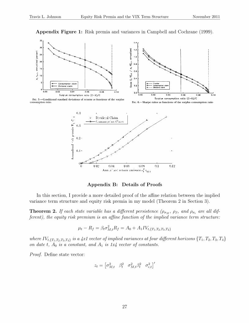
(C − X)/C. Figures 5 and 6 in Campbell and Cochrane (1999), reproduced in AppendixFigure 1, show that the shape of the Sharpe Ratio as a function of surplus consumption isnearly identical to the shape of the conditional standard deviation. Dividing the conditionalSharpe Ratio by the conditional standard deviation yields the ratio of equity risk premia toconditional variance, so the similarity of the plots in Figures 5 and 6 suggest that this ratiois close to constant across states in the Campbell and Cochrane (1999) model.
Appendix Figure 1 shows the relation between conditional variance and risk premia inCampbell and Cochrane (1999) for both the consumption claim and the dividend claim.For both assets, the relation is nearly linear, indicating that equity risk premia are almostperfectly correlated with conditional variance in the model. Note that the dividend claimis to the right of the consumption claim in this plot because of the additional variance individend growth that is independent of the SDF, and therefore has no bearing on expectedreturns.
26
Travis L. Johnson Equity Risk Premia and the VIX Term Structure November 2011
Appendix Figure 1: Risk premia and variances in Campbell and Cochrane (1999).
Appendix B: Details of Proofs
In this section, I provide a more detailed proof of the affine relation between the impliedvariance term structure and equity risk premia in my model (Theorem 2 in Section 3).
Theorem 2. If each state variable has a different persistence (ρσM , ρβ, and ρσε are all dif-ferent), the equity risk premium is an affine function of the implied variance term structure:
µt −Rf = βtσ2M,tRf = A0 + A1IVt,{T1,T2,T3,T4}
where IVt,{T1,T2,T3,T4} is a 4x1 vector of implied variances at four different horizons {T1, T2, T3, T4}on date t, A0 is a constant, and A1 is 1x4 vector of constants.
Proof. Define state vector:
zt =[σ2M,t β2
t σ2M,tβ
2t σ2
ε,t
]′
27
Travis L. Johnson Equity Risk Premia and the VIX Term Structure November 2011
The equity risk premium µt −Rf is an affine function of the state vector zt since:
µt −Rf = βtσ2M,tRf
=
(β2t + βHβLβH + βL
)σ2M,tRf
=[RfβhβLβH+βL
0Rf
βH+βL0]
︸ ︷︷ ︸b1
zt
The second line relies on the discreteness of βt, which implies that βt =β2t+βHβLβH+βL
. Thisequation does not hold for continuous βt. However, Theorem 2 is not an artifact of thediscreteness. As discussed in Appendix C, the same result holds in the continuous case butrequires 6 horizons of the VIX term structure rather than 4.
The implied variance measure IVt,T is also an affine function of the state vector zt.Starting from the definition in Equation (12):
IVt,T =1
T
T−1∑s=0
EQt (σ
2R,t+s)
Since the variance states are independent of the SDF and eachother, we have that:
EQt (σ
2R,t+s) = Et(β
2t+s)Et(σ
2M,t+s) + Et(σ
2ε,t+s)
Since each state variable is an AR(1), we have:
Et(σ2M,t+s) = σ2
M + ρsσM (σ2M,t − σ2
M)
Et(β2t+s) = β2 + ρsβ(β
2t − β2)
Et(σ2ε,t+s) = σ2
ε + ρsσε(σ2ε,t − σ2
ε )
where σ2M , β2, and σ2
ε are unconditional means. Putting these together yields:
EQt (σ
2R,t+s) = d0(s) + d1(s)zt
d0(s) = β2(1− ρsβ)σ2M(1− ρsσM ) + σ2
ε (1− ρ2σε)
d1(s) =[β2ρsσM (1− ρ
sβ) σ2
Mρsβ(1− ρsσM ) ρsσMρ
sβ ρsσε
]⇒ IVt,T =
1
T
T−1∑s=0
d0(s) +
(1
T
T−1∑s=0
d1(s)
)zt = c0(T ) + c1(T )zt
28
Travis L. Johnson Equity Risk Premia and the VIX Term Structure November 2011
These coefficients can be summed using the geometric series summation∑T−1
s=0 aρs = a1−ρT
1−ρ :
c0(T ) =1
T
(β2σ2
M
(1−
1− ρTσM1− ρσM
−1− ρTβ1− ρβ
+1− ρTσMρ
Tβ
1− ρσMρβ
)+ σ2
ε
(1−
1− ρTσε1− ρσε
))
c1(T ) =1
T
[β2
(1−ρTβ1−ρβ
− 1−ρTσM ρTβ1−ρσM ρβ
)σ2M
(1−ρTβ1−ρβ
− 1−ρTσM ρTβ1−ρσM ρβ
)1−ρTσM ρTβ1−ρσM ρβ
1−ρTσε1−ρσε
]The implied variance term structure IVt,{T1,T2,T3,T4} is also an affine function of zt:
IVt,{T1,T2,T3,T4} =
c0(T1)c0(T2)c0(T3)c0(T4)
︸ ︷︷ ︸
C0
+
c1(T1)c1(T2)c1(T3)c1(T4)
︸ ︷︷ ︸
C1
zt
As long as the VIX term structure is composed of four different horizons, and the threepersistences ρσM , ρβ, and ρσε are all different, C1 is invertible since each column of C1 changesat a different rate with respect to T , the only thing changing across rows of C1. Therefore,the risk premia can be computed from the implied variance term structure as follows:
zt = C−11
(IVt,{T1,T2,T3,T4} − C0
)⇒ µt −Rf = b1C
−11
(IVt,{T1,T2,T3,T4} − C0
)(19)
Appendix C: Continuous version of the model
This appendix contains a continuous-time, continuous-state, analogue to the model inSection 3. The intuition and main results are identical, indicating that the stark discretenessin the main model is not driving any of the results.
The following differential equation governs the stochastic discount factor (SDF) mt:
dmt
mt
= −rtdt+√vmt dB
mt (20)
where rt is the risk-free rate process, which I fix at r to keep the focus away from theterm structure of interest rates, and
√vmt is the SDF’s diffusion process, which follows the
square-root process used in Heston (1993) and Cox, Ingersoll, and Ross (1985):
dvmt = κvm(θvm − vmt )dt+ σvm√vmt dB
vmt (21)
The parameter κvm represents the extent of mean reversion in vmt , with higher values resultingin more mean reversion and therefore less persistence. The parameters θvm and σvm allowthe unconditional mean and variance of vmt to be any non-negative number. The Brownian
29
Travis L. Johnson Equity Risk Premia and the VIX Term Structure November 2011
motion Bvmt has correlation ρvm,m with the SDF.7 In the data, we observe that innovations
in the VIX and the equity market have a strong negative correlation (the so-called leverageeffect), which suggests a positive correlation ρvm,m > 0 between innovations in m and vm.
There is also a traded asset with value St, which is also correlated with innovations inmt, as dictated by the process:
dStSt
= µtdt+√vRt
(ρS,tdB
mt +
√1− ρ2S,tdB
εt
)(22)
= µtdt− βt√vmt dB
mt +
√vεtdB
εt (23)
Where vRt is the diffusion of log(St), βt = −ρs,t√
vRtvmt
, and vεt = vRt − β2t v
mt . I proceed with
(23) because it isolates the SDF diffusion√vmt , which is already specified by Equation (21).
Since the returns of procyclical risky assets are negatively correlated with the SDF, ρt isnegative for these assets and βt is positive.
Since mt is a stochastic discount factor, no arbitrage implies that:
µt = r + βtvmt . (24)
The three state variables have the following interpretations: vmt is the variance of the SDF,βt is the SDF beta, and vεt the variance of the part of returns orthogonal to the SDF, orunpriced risk. These three quantities are discussed in more detail throughout the paper.
Both βt and vεt also follow square-root processes:
dβt = κβ(θβ − βt)dt+ σβ√βtdB
βt (25)
dvεt = κvε(θvε − vεt)dt+ σvε√vεtdB
vεt (26)
These parallel vmt with the exception that they are uncorrelated with the SDF. In reality,innovations in both the SDF beta and unpriced risk could be correlated with the SDF, butby ignoring these correlations I can use the pairwise independence of (vmt , βt, vεt) to computemany cross-moments like Et(β2
TvT ) that would otherwise be intractable. Additionally, whilethe correlation between the SDF and volatility generates the leverage effect and volatilityrisk premium in the model, it has little effect on the incremental value of the volatility termstructure in identifying risk premia.
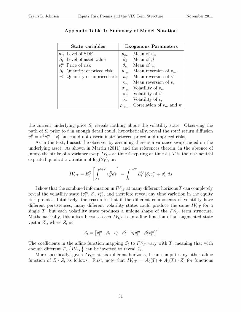
Appendix Table 1 summarizes the ten exogenous parameters and five state variables ofthe model. Two of the state variables, the SDF level mt and asset price level St, have noimpact on the distribution of future log returns. The other three state variables are allstationary and Markov, allowing the computation of both conditional and unconditionalmoments.
3.1. Risk and Return in the ModelWhile the marginal investor knows their preferences and the distribution of asset values,
and can therefore compute the three volatility states vmt , βt, and vεt , I study the problem of anoutsider observer that tries to infer the state using traded asset prices. For such an observer,
7Formally, dBvmt = ρvm,mdBmt +
√1− ρ2vm,mdB
ε,vmt where Bε,vmt is an independent Brownian motion.
30
Travis L. Johnson Equity Risk Premia and the VIX Term Structure November 2011
Appendix Table 1: Summary of Model Notation
State variables Exogenous Parameters
mt Level of SDF θvm Mean of vmSt Level of asset value θβ Mean of βvmt Price of risk θvε Mean of vεβt Quantity of priced risk κvm Mean reversion of vmvεt Quantity of unpriced risk κβ Mean reversion of β
κvε Mean reversion of vεσvm Volatility of vmσβ Volatility of βσvε Volatility of vερvm,m Correlation of vm and m
the current underlying price St reveals nothing about the volatility state. Observing thepath of St prior to t in enough detail could, hypothetically, reveal the total return diffusionvRt = β2
t vmt + vεt but could not discriminate between priced and unpriced risks.
As in the text, I assist the observer by assuming there is a variance swap traded on theunderlying asset. As shown in Martin (2011) and the references therein, in the absence ofjumps the strike of a variance swap IVt,T at time t expiring at time t+ T is the risk-neutralexpected quadratic variation of log(ST ), or:
IVt,T = EQt
[∫ t+T
t
vRs ds
]=
∫ t+T
t
EQt [βsv
ms + vεs] ds
I show that the combined information in IVt,T at many different horizons T can completelyreveal the volatility state (vmt , βt, vεt), and therefore reveal any time variation in the equityrisk premia. Intuitively, the reason is that if the different components of volatility havedifferent persistences, many different volatility states could produce the same IVt,T for asingle T , but each volatility state produces a unique shape of the IVt,T term structure.Mathematically, this arises because each IVt,T is an affine function of an augmented statevector Zt, where Zt is:
Zt =[vmt βt vεt β2
t βtvmt β2
t vmt
]′The coefficients in the affine function mapping Zt to IVt,T vary with T , meaning that withenough different T ,
{IVt,T
}can be inverted to reveal Zt.
More specifically, given IVt,T at six different horizons, I can compute any other affinefunction of B · Zt as follows. First, note that IVt,T = A0(T ) + A1(T ) · Zt for functions
31
Travis L. Johnson Equity Risk Premia and the VIX Term Structure November 2011
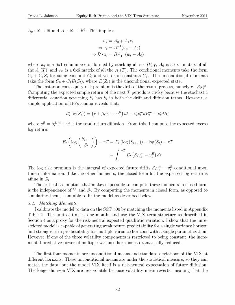
A0 : R→ R and A1 : R→ R6. This implies:
wt = A0 + A1zt
⇒ zt = A−11 (wt − A0)
⇒ B · zt = BA−11 (wt − A0)
where wt is a 6x1 column vector formed by stacking all six IVt,T , A0 is a 6x1 matrix of allthe A0(T ), and A1 is a 6x6 matrix of all the A1(T ). The conditional moments take the formC0 + C1Zt for some constant C0 and vector of constants C1. The unconditional momentstake the form C0 + C1E(Zt), where E(Zt) is the unconditional expected state.
The instantaneous equity risk premium is the drift of the return process, namely r+βtvmt .Computing the expected simple return of the next T periods is tricky because the stochasticdifferential equation governing St has St in both the drift and diffusion terms. However, asimple application of Ito’s lemma reveals that:
d(log(St)) =(r + βtv
mt − vRt
)dt− βtvmt dBm
t + vεtdBεt
where vRt = β2t v
mt +vεt is the total return diffusion. From this, I compute the expected excess
log return:
Et
(log
(St+TSt
))− rT = Et (log (St+T ))− log(St)− rT
=
∫ t+T
t
Et(βsv
ms − vRs
)ds
The log risk premium is the integral of expected future drifts βsvms − vRs conditional upontime t information. Like the other moments, the closed form for the expected log return isaffine in Zt.
The critical assumption that makes it possible to compute these moments in closed formis the independence of Vt and βt. By computing the moments in closed form, as opposed tosimulating them, I am able to fit the model as described below.
3.2. Matching MomentsI calibrate the model to data on the S&P 500 by matching the moments listed in Appendix
Table 2. The unit of time is one month, and use the VIX term structure as described inSection 4 as a proxy for the risk-neutral expected quadratic variation. I show that the unre-stricted model is capable of generating weak return predictability for a single variance horizonand strong return predictability for multiple variance horizons with a single parametrization.However, if one of the three volatility components is restricted to being constant, the incre-mental predictive power of multiple variance horizons is dramatically reduced.
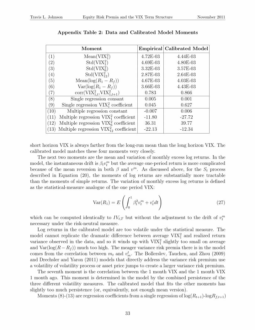
The first four moments are unconditional means and standard deviations of the VIX atdifferent horizons. These unconditional means are under the statistical measure, so they canmatch the data, but the model VIX itself is a risk-neutral expectation of future diffusion.The longer-horizon VIX are less volatile because volatility mean reverts, meaning that the
32
Travis L. Johnson Equity Risk Premia and the VIX Term Structure November 2011
Appendix Table 2: Data and Calibrated Model Moments
Moment Empirical Calibrated Model
(1) Mean(VIX21) 4.72E-03 4.44E-03
(2) Std(VIX21) 4.69E-03 4.80E-03
(3) Std(VIX26) 3.32E-03 3.57E-03
(4) Std(VIX212) 2.87E-03 2.64E-03
(5) Mean(log(R1 −Rf )) 4.67E-03 4.03E-03(6) Var(log(R1 −Rf )) 3.66E-03 4.43E-03(7) corr(VIX2
1,t,VIX21,t+1) 0.783 0.866
(8) Single regression consant 0.005 0.001(9) Single regression VIX2
1 coefficient 0.045 0.627(10) Multiple regression constant -0.007 0.006(11) Multiple regression VIX2
1 coefficient -11.80 -27.72(12) Multiple regression VIX2
6 coefficient 36.31 39.77(13) Multiple regression VIX2
12 coefficient -22.13 -12.34
short horizon VIX is always farther from the long-run mean than the long horizon VIX. Thecalibrated model matches these four moments very closely.
The next two moments are the mean and variation of monthly excess log returns. In themodel, the instantaneous drift is βtvmt but the average one-period return is more complicatedbecause of the mean reversion in both β and vm. As discussed above, for the St processdescribed in Equation (20), the moments of log returns are substantially more tractablethan the moments of simple returns. The variation of monthly excess log returns is definedas the statistical-measure analogue of the one period VIX:
Var(R1) = E
(∫ 1
0
β2t v
mt + vεtdt
)(27)
which can be computed identically to IVt,T but without the adjustment to the drift of vmtnecessary under the risk-neutral measure.
Log returns in the calibrated model are too volatile under the statistical measure. Themodel cannot replicate the dramatic difference between average VIX2
1 and realized returnvariance observed in the data, and so it winds up with VIX2
1 slightly too small on averageand Var(log(R−Rf )) much too high. The meager variance risk premia there is in the modelcomes from the correlation between mt and vtm. The Bollerslev, Tauchen, and Zhou (2009)and Drechsler and Yaron (2011) models that directly address the variance risk premium usea volatility of volatility process or asset price jumps to create a larger variance risk premium.
The seventh moment is the correlation between the 1 month VIX and the 1 month VIX1 month ago. This moment is determined in the model by the combined persistence of thethree different volatility measures. The calibrated model that fits the other moments hasslightly too much persistence (or, equivalently, not enough mean version).
Moments (8)-(13) are regression coefficients from a single regression of log(Rt+1)-logRf,t+1)
33
Travis L. Johnson Equity Risk Premia and the VIX Term Structure November 2011
on a constant and VIX1,t; and a multiple regression of log(Rt+1)-log(Rf,t+1) on a constant,VIX1,t, VIX6,t, and VIX12,t. The calibrated model matches the nearly 0 intercepts, weaklypositive single regression slope coefficient, as well as the tent shape of the multiple regressioncoefficients. However, the single regression slope coefficient is considerably higher in thecalibrated model than the data.
34
Travis L. Johnson Equity Risk Premia and the VIX Term Structure November 2011
References
Bansal, Ravi and Amir Yaron, 2004, Risks for the long run: A potential resolution of assetpricing puzzles, The Journal of Finance 59, 1481–1509.
Bloom, Nicholas, 2009, The impact of uncertainty shocks, Econometrica 77, 623–685.
Bollerslev, Tim, George Tauchen, and Hau Zhou, 2009, Expected stock returns and variancerisk premia, Review of Financial Studies 22, 4463.
Boudoukh, Jacob, Roni Michaely, Matthew Richardson, and Michael R. Roberts, 2007, Onthe importance of measuring payout yield: Implications for empirical asset pricing, TheJournal of Finance 62, 877–915.
Breeden, Douglas T. and Robert H. Litzenberger, 1978, Prices of state-contingent claimsimplicit in option prices, Journal of Business 621–651.
Britten-Jones, Mark and Anthony Neuberger, 2000, Option prices, implied price processes,and stochastic volatility, The Journal of Finance 55, 839–866.
Campbell, John Y. and John H. Cochrane, 1999, By force of habit: A consumption-basedexplanation of aggregate stock market behavior, The Journal of Political Economy 107,205–251.
Campbell, John Y. and Robert J. Shiller, 1988, The dividend-price ratio and expectationsof future dividends and discount factors, Review of Financial Studies 1, 195–228.
Carr, Peter and D. Madan, 1998, Towards a theory of volatility trading, Option Pricing,Interest Rates, and Risk Management 417–427.
Christoffersen, Peter., Steven Heston, and Kris Jacobs, 2009, The shape and term structureof the index option smirk: Why multifactor stochastic volatility models work so well,Management Science 55, 1914–1932.
Cochrane, John H., 2008, The dog that did not bark: A defense of return predictability,Review of Financial Studies 21, 1533–1575.
Cochrane, John H. and Monika Piazzesi, 2005, Bond Risk Premia, The American EconomicReview 95, 138–160.
Cochrane, John H. and Monika Piazzesi, 2008, Decomposing the yield curve, University ofChicago Working Paper .
Cox, John C., Jonathan E. Ingersoll, and Stephen A. Ross, 1985, A theory of the termstructure of interest rates, Econometrica 53, 385–407.
Dai, Qiang and Kenneth J. Singleton, 2002, Expectation puzzles, time-varying risk premia,and affine models of the term structure, Journal of Financial Economics 63, 415–441.
35
Travis L. Johnson Equity Risk Premia and the VIX Term Structure November 2011
Drechsler, Itamar and Amir Yaron, 2011, What’s vol got to do with it, Review of FinancialStudies 24, 1.
Duan, Jin-Chuan and Chung-Ying Yeh, 2011, Price and volatility dynamics implied by thevix term structure, National University of Singapore Working Paper .
Heston, Steven L., 1993, A closed-form solution for options with stochastic volatility withapplications to bond and currency options, Review of Financial Studies 6, 327.
Jiang, George J. and Yisong S. Tian, 2005, The model-free implied volatility and its infor-mation content, Review of Financial Studies 18, 1305.
Martin, Ian, 2011, Simple variance swaps, Stanford University Working Paper .
Mixon, Scott, 2007, The implied volatility term structure of stock index options, Journal ofEmpirical Finance 14, 333–354.
Neuberger, Anthony, 1994, The log contract, The Journal of Portfolio Management 20,74–80.
Sepp, Artur, 2008, Vix option pricing in a jump-diffusion model, Risk Magazine 84–89.
Stambaugh, Robert F., 1999, Predictive regressions, Journal of Financial Economics 54,421.
Zhu, Yingzi and Jin E. Zhang, 2007, Variance term structure and vix futures pricing, Inter-national Journal of Theoretical and Applied Finance 10, 111.
36
Travis L. Johnson Equity Risk Premia and the VIX Term Structure November 2011
Figure 1: Model Equity Risk Premia and the VIX Term Structure
Figure 1 shows the VIX term structure, and corresponding equity risk premia, in each possiblestate of the world in my calibrated model. The VIX term structure is presented as an annualizedstandard deviation. The equity risk premia, presented to the left of each curve, are also annualized.The model and its calibration are described in Section 4 and Table 1.
37
Travis L. Johnson Equity Risk Premia and the VIX Term Structure November 2011
Figure 2: Functions integrated to compute VIX212 on January 2nd, 1996.
Figure 2 presents the functions integrated when computing the twelve-month VIX2 on the first dayin my sample, January 2nd, 1996. Each function is the integrand of equation (14) in Section 4 ofthe paper. As described in the text, these functions are numerically integrated across the range ofavailable strike prices, and interpolated to estimate the twelve-month VIX2.
38
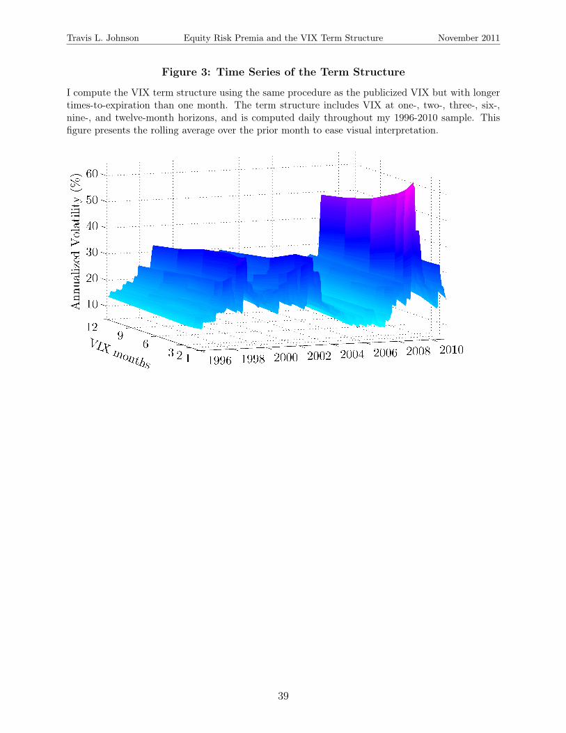
Travis L. Johnson Equity Risk Premia and the VIX Term Structure November 2011
Figure 3: Time Series of the Term Structure
I compute the VIX term structure using the same procedure as the publicized VIX but with longertimes-to-expiration than one month. The term structure includes VIX at one-, two-, three-, six-,nine-, and twelve-month horizons, and is computed daily throughout my 1996-2010 sample. Thisfigure presents the rolling average over the prior month to ease visual interpretation.
39
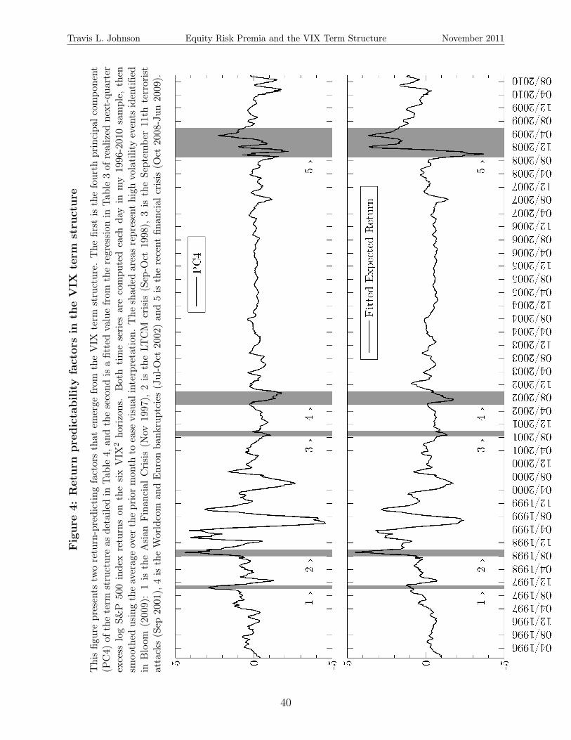
Travis L. Johnson Equity Risk Premia and the VIX Term Structure November 2011
Fig
ure
4:R
eturn
pre
dic
tability
fact
ors
inth
eV
IXte
rmst
ruct
ure
Thisfig
urepresents
tworeturn-predictingfactorsthat
emerge
from
theVIX
term
structure.
The
first
isthefourth
principa
lcom
pone
nt(P
C4)
oftheterm
structureas
detaile
din
Tab
le4,
andthesecond
isafittedvaluefrom
theregression
inTab
le3of
realized
next-qua
rter
excess
logS&
P50
0inde
xreturnson
thesixVIX
2ho
rizons.
Bothtimeseries
arecompu
tedeach
dayin
my1996-2010sample,
then
smoo
thed
usingtheaverag
eover
thepriormon
thto
ease
visual
interpretation
.The
shad
edareasrepresenthigh
volatilityevents
identifie
din
Bloom
(200
9):1is
theAsian
Finan
cial
Crisis(N
ov19
97),
2is
theLT
CM
crisis
(Sep
-Oct
1998
),3is
theSe
ptem
ber11th
terrorist
attacks(Sep
2001
),4is
theWorldcom
andEnron
bank
ruptcies
(Jul-O
ct20
02)an
d5is
therecent
finan
cial
crisis
(Oct
2008-Jun
2009).
40
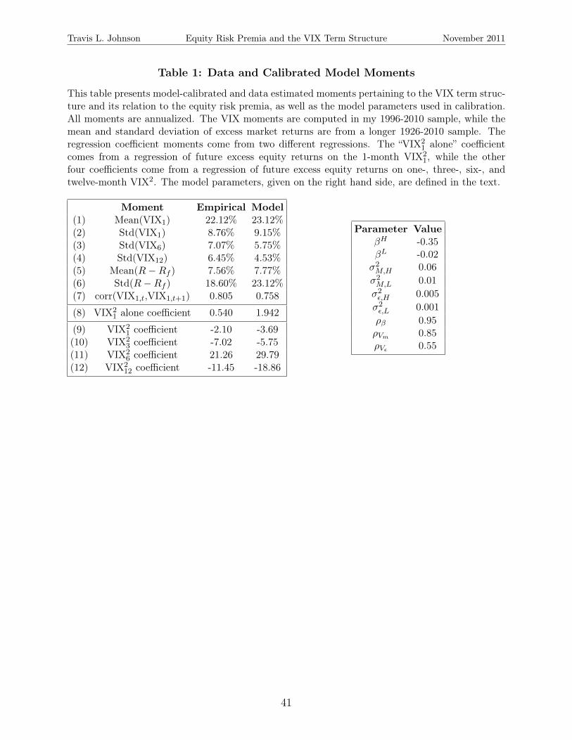
Travis L. Johnson Equity Risk Premia and the VIX Term Structure November 2011
Table 1: Data and Calibrated Model Moments
This table presents model-calibrated and data estimated moments pertaining to the VIX term struc-ture and its relation to the equity risk premia, as well as the model parameters used in calibration.All moments are annualized. The VIX moments are computed in my 1996-2010 sample, while themean and standard deviation of excess market returns are from a longer 1926-2010 sample. Theregression coefficient moments come from two different regressions. The “VIX2
1 alone” coefficientcomes from a regression of future excess equity returns on the 1-month VIX2
1, while the otherfour coefficients come from a regression of future excess equity returns on one-, three-, six-, andtwelve-month VIX2. The model parameters, given on the right hand side, are defined in the text.
Moment Empirical Model(1) Mean(VIX1) 22.12% 23.12%(2) Std(VIX1) 8.76% 9.15%(3) Std(VIX6) 7.07% 5.75%(4) Std(VIX12) 6.45% 4.53%(5) Mean(R−Rf ) 7.56% 7.77%(6) Std(R−Rf ) 18.60% 23.12%(7) corr(VIX1,t,VIX1,t+1) 0.805 0.758
(8) VIX21 alone coefficient 0.540 1.942
(9) VIX21 coefficient -2.10 -3.69
(10) VIX23 coefficient -7.02 -5.75
(11) VIX26 coefficient 21.26 29.79
(12) VIX212 coefficient -11.45 -18.86
Parameter ValueβH -0.35βL -0.02σ2M,H 0.06σ2M,L 0.01σ2ε,H 0.005σ2ε,L 0.001ρβ 0.95ρVm 0.85ρVε 0.55
41
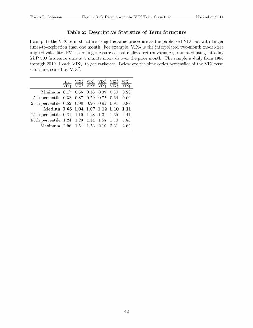
Travis L. Johnson Equity Risk Premia and the VIX Term Structure November 2011
Table 2: Descriptive Statistics of Term Structure
I compute the VIX term structure using the same procedure as the publicized VIX but with longertimes-to-expiration than one month. For example, VIX2 is the interpolated two-month model-freeimplied volatility. RV is a rolling measure of past realized return variance, estimated using intradayS&P 500 futures returns at 5-minute intervals over the prior month. The sample is daily from 1996through 2010. I each VIXT to get variances. Below are the time-series percentiles of the VIX termstructure, scaled by VIX2
1.
RVVIX2
1
VIX22
VIX21
VIX23
VIX21
VIX26
VIX21
VIX29
VIX21
VIX212
VIX21
Minimum 0.17 0.66 0.36 0.39 0.30 0.235th percentile 0.38 0.87 0.79 0.72 0.64 0.6025th percentile 0.52 0.98 0.96 0.95 0.91 0.88
Median 0.65 1.04 1.07 1.12 1.10 1.1175th percentile 0.81 1.10 1.18 1.31 1.35 1.4195th percentile 1.24 1.20 1.34 1.58 1.70 1.80
Maximum 2.96 1.54 1.73 2.10 2.31 2.69
42
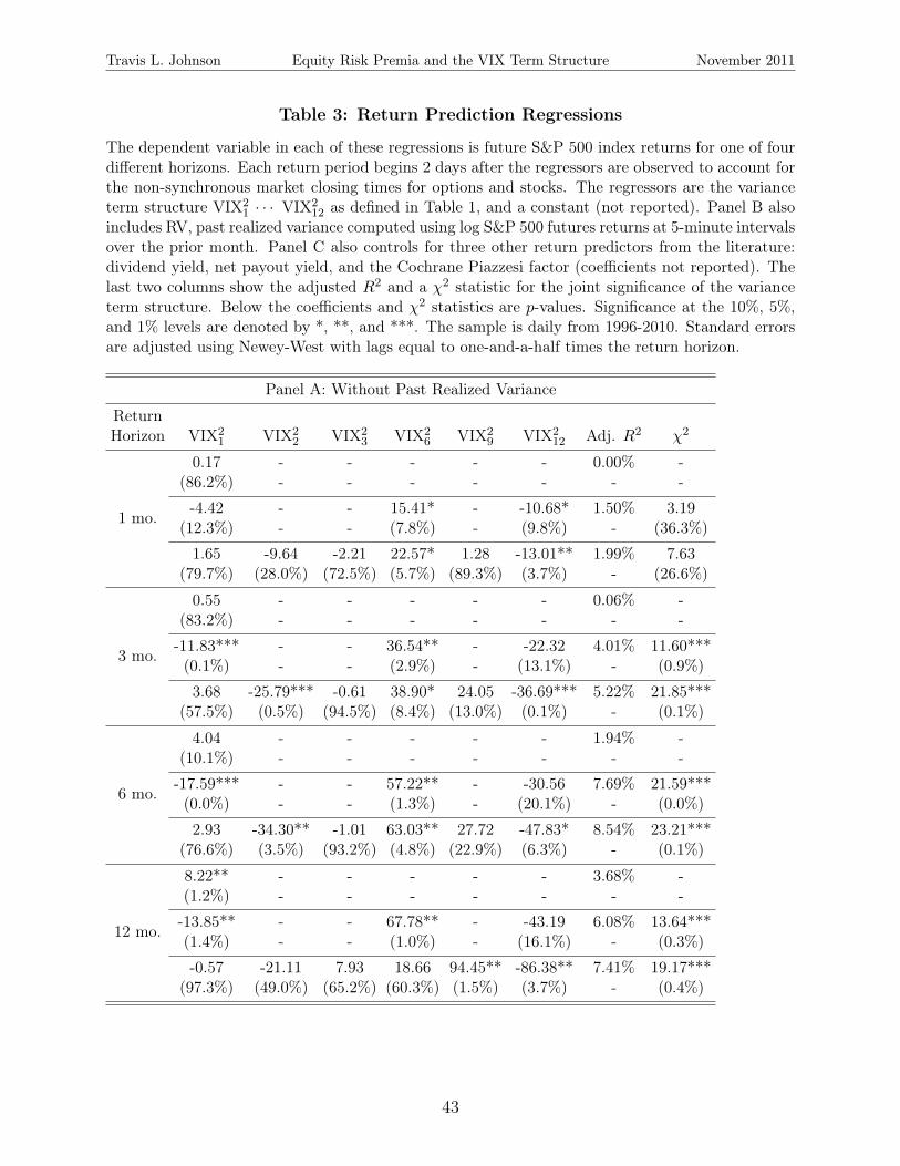
Travis L. Johnson Equity Risk Premia and the VIX Term Structure November 2011
Table 3: Return Prediction Regressions
The dependent variable in each of these regressions is future S&P 500 index returns for one of fourdifferent horizons. Each return period begins 2 days after the regressors are observed to account forthe non-synchronous market closing times for options and stocks. The regressors are the varianceterm structure VIX2
1 · · · VIX212 as defined in Table 1, and a constant (not reported). Panel B also
includes RV, past realized variance computed using log S&P 500 futures returns at 5-minute intervalsover the prior month. Panel C also controls for three other return predictors from the literature:dividend yield, net payout yield, and the Cochrane Piazzesi factor (coefficients not reported). Thelast two columns show the adjusted R2 and a χ2 statistic for the joint significance of the varianceterm structure. Below the coefficients and χ2 statistics are p-values. Significance at the 10%, 5%,and 1% levels are denoted by *, **, and ***. The sample is daily from 1996-2010. Standard errorsare adjusted using Newey-West with lags equal to one-and-a-half times the return horizon.
Panel A: Without Past Realized Variance
ReturnHorizon VIX2
1 VIX22 VIX2
3 VIX26 VIX2
9 VIX212 Adj. R2 χ2
1 mo.
0.17 - - - - - 0.00% -(86.2%) - - - - - - -
-4.42 - - 15.41* - -10.68* 1.50% 3.19(12.3%) - - (7.8%) - (9.8%) - (36.3%)
1.65 -9.64 -2.21 22.57* 1.28 -13.01** 1.99% 7.63(79.7%) (28.0%) (72.5%) (5.7%) (89.3%) (3.7%) - (26.6%)
3 mo.
0.55 - - - - - 0.06% -(83.2%) - - - - - - -
-11.83*** - - 36.54** - -22.32 4.01% 11.60***(0.1%) - - (2.9%) - (13.1%) - (0.9%)
3.68 -25.79*** -0.61 38.90* 24.05 -36.69*** 5.22% 21.85***(57.5%) (0.5%) (94.5%) (8.4%) (13.0%) (0.1%) - (0.1%)
6 mo.
4.04 - - - - - 1.94% -(10.1%) - - - - - - -
-17.59*** - - 57.22** - -30.56 7.69% 21.59***(0.0%) - - (1.3%) - (20.1%) - (0.0%)
2.93 -34.30** -1.01 63.03** 27.72 -47.83* 8.54% 23.21***(76.6%) (3.5%) (93.2%) (4.8%) (22.9%) (6.3%) - (0.1%)
12 mo.
8.22** - - - - - 3.68% -(1.2%) - - - - - - -
-13.85** - - 67.78** - -43.19 6.08% 13.64***(1.4%) - - (1.0%) - (16.1%) - (0.3%)
-0.57 -21.11 7.93 18.66 94.45** -86.38** 7.41% 19.17***(97.3%) (49.0%) (65.2%) (60.3%) (1.5%) (3.7%) - (0.4%)
43
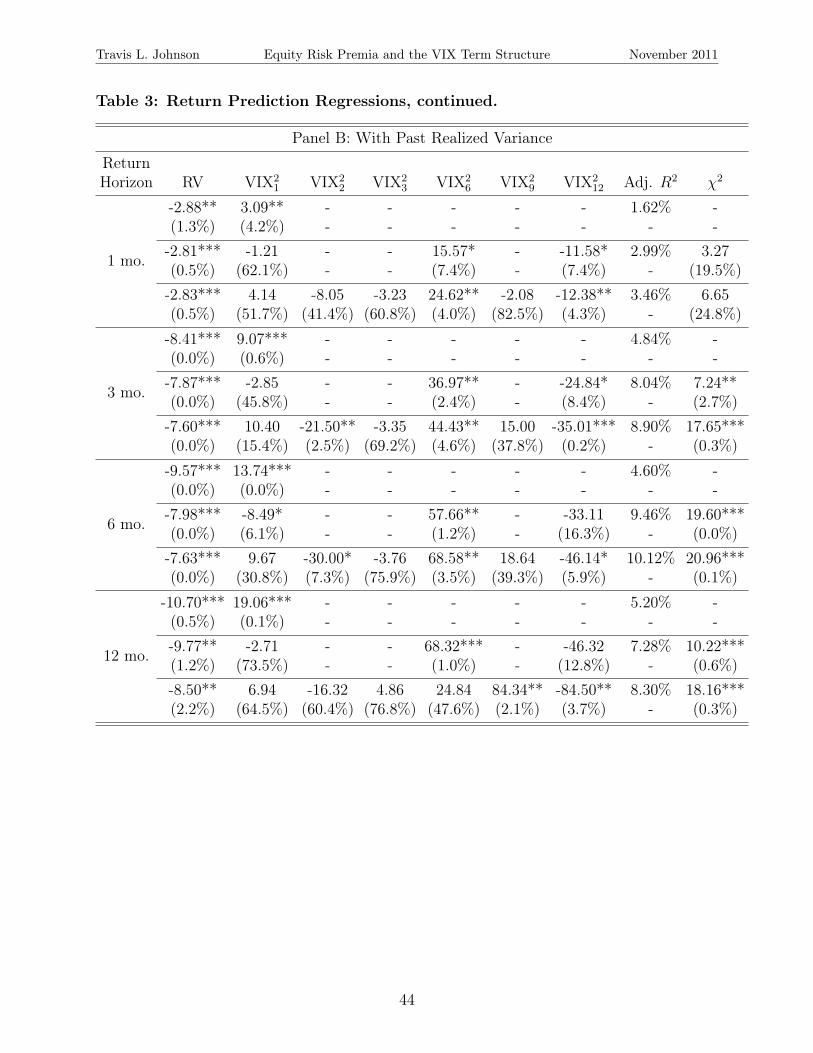
Travis L. Johnson Equity Risk Premia and the VIX Term Structure November 2011
Table 3: Return Prediction Regressions, continued.
Panel B: With Past Realized VarianceReturnHorizon RV VIX2
1 VIX22 VIX2
3 VIX26 VIX2
9 VIX212 Adj. R2 χ2
1 mo.
-2.88** 3.09** - - - - - 1.62% -(1.3%) (4.2%) - - - - - - --2.81*** -1.21 - - 15.57* - -11.58* 2.99% 3.27(0.5%) (62.1%) - - (7.4%) - (7.4%) - (19.5%)-2.83*** 4.14 -8.05 -3.23 24.62** -2.08 -12.38** 3.46% 6.65(0.5%) (51.7%) (41.4%) (60.8%) (4.0%) (82.5%) (4.3%) - (24.8%)
3 mo.
-8.41*** 9.07*** - - - - - 4.84% -(0.0%) (0.6%) - - - - - - --7.87*** -2.85 - - 36.97** - -24.84* 8.04% 7.24**(0.0%) (45.8%) - - (2.4%) - (8.4%) - (2.7%)-7.60*** 10.40 -21.50** -3.35 44.43** 15.00 -35.01*** 8.90% 17.65***(0.0%) (15.4%) (2.5%) (69.2%) (4.6%) (37.8%) (0.2%) - (0.3%)
6 mo.
-9.57*** 13.74*** - - - - - 4.60% -(0.0%) (0.0%) - - - - - - --7.98*** -8.49* - - 57.66** - -33.11 9.46% 19.60***(0.0%) (6.1%) - - (1.2%) - (16.3%) - (0.0%)-7.63*** 9.67 -30.00* -3.76 68.58** 18.64 -46.14* 10.12% 20.96***(0.0%) (30.8%) (7.3%) (75.9%) (3.5%) (39.3%) (5.9%) - (0.1%)
12 mo.
-10.70*** 19.06*** - - - - - 5.20% -(0.5%) (0.1%) - - - - - - --9.77** -2.71 - - 68.32*** - -46.32 7.28% 10.22***(1.2%) (73.5%) - - (1.0%) - (12.8%) - (0.6%)-8.50** 6.94 -16.32 4.86 24.84 84.34** -84.50** 8.30% 18.16***(2.2%) (64.5%) (60.4%) (76.8%) (47.6%) (2.1%) (3.7%) - (0.3%)
44
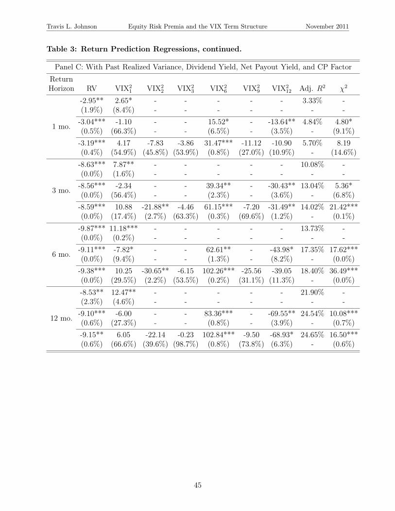
Travis L. Johnson Equity Risk Premia and the VIX Term Structure November 2011
Table 3: Return Prediction Regressions, continued.
Panel C: With Past Realized Variance, Dividend Yield, Net Payout Yield, and CP FactorReturnHorizon RV VIX2
1 VIX22 VIX2
3 VIX26 VIX2
9 VIX212 Adj. R2 χ2
1 mo.
-2.95** 2.65* - - - - - 3.33% -(1.9%) (8.4%) - - - - - - --3.04*** -1.10 - - 15.52* - -13.64** 4.84% 4.80*(0.5%) (66.3%) - - (6.5%) - (3.5%) - (9.1%)-3.19*** 4.17 -7.83 -3.86 31.47*** -11.12 -10.90 5.70% 8.19(0.4%) (54.9%) (45.8%) (53.9%) (0.8%) (27.0%) (10.9%) - (14.6%)
3 mo.
-8.63*** 7.87** - - - - - 10.08% -(0.0%) (1.6%) - - - - - - --8.56*** -2.34 - - 39.34** - -30.43** 13.04% 5.36*(0.0%) (56.4%) - - (2.3%) - (3.6%) - (6.8%)-8.59*** 10.88 -21.88** -4.46 61.15*** -7.20 -31.49** 14.02% 21.42***(0.0%) (17.4%) (2.7%) (63.3%) (0.3%) (69.6%) (1.2%) - (0.1%)
6 mo.
-9.87*** 11.18*** - - - - - 13.73% -(0.0%) (0.2%) - - - - - - --9.11*** -7.82* - - 62.61** - -43.98* 17.35% 17.62***(0.0%) (9.4%) - - (1.3%) - (8.2%) - (0.0%)-9.38*** 10.25 -30.65** -6.15 102.26*** -25.56 -39.05 18.40% 36.49***(0.0%) (29.5%) (2.2%) (53.5%) (0.2%) (31.1%) (11.3%) - (0.0%)
12 mo.
-8.53** 12.47** - - - - - 21.90% -(2.3%) (4.6%) - - - - - - --9.10*** -6.00 - - 83.36*** - -69.55** 24.54% 10.08***(0.6%) (27.3%) - - (0.8%) - (3.9%) - (0.7%)-9.15** 6.05 -22.14 -0.23 102.84*** -9.50 -68.93* 24.65% 16.50***(0.6%) (66.6%) (39.6%) (98.7%) (0.8%) (73.8%) (6.3%) - (0.6%)
45
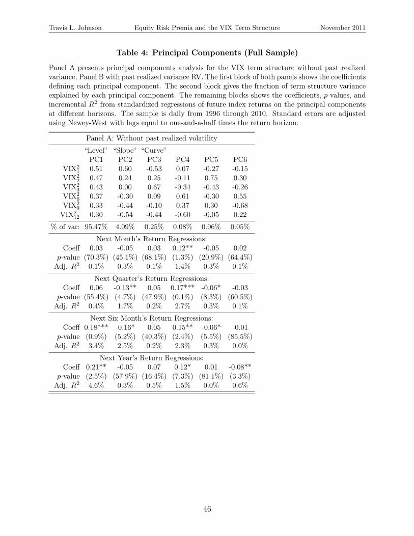
Travis L. Johnson Equity Risk Premia and the VIX Term Structure November 2011
Table 4: Principal Components (Full Sample)
Panel A presents principal components analysis for the VIX term structure without past realizedvariance, Panel B with past realized variance RV. The first block of both panels shows the coefficientsdefining each principal component. The second block gives the fraction of term structure varianceexplained by each principal component. The remaining blocks shows the coefficients, p-values, andincremental R2 from standardized regressions of future index returns on the principal componentsat different horizons. The sample is daily from 1996 through 2010. Standard errors are adjustedusing Newey-West with lags equal to one-and-a-half times the return horizon.
Panel A: Without past realized volatility
“Level” “Slope” “Curve”PC1 PC2 PC3 PC4 PC5 PC6
VIX21 0.51 0.60 -0.53 0.07 -0.27 -0.15
VIX22 0.47 0.24 0.25 -0.11 0.75 0.30
VIX23 0.43 0.00 0.67 -0.34 -0.43 -0.26
VIX26 0.37 -0.30 0.09 0.61 -0.30 0.55
VIX29 0.33 -0.44 -0.10 0.37 0.30 -0.68
VIX212 0.30 -0.54 -0.44 -0.60 -0.05 0.22
% of var: 95.47% 4.09% 0.25% 0.08% 0.06% 0.05%
Next Month’s Return Regressions:Coeff 0.03 -0.05 0.03 0.12** -0.05 0.02
p-value (70.3%) (45.1%) (68.1%) (1.3%) (20.9%) (64.4%)Adj. R2 0.1% 0.3% 0.1% 1.4% 0.3% 0.1%
Next Quarter’s Return Regressions:Coeff 0.06 -0.13** 0.05 0.17*** -0.06* -0.03
p-value (55.4%) (4.7%) (47.9%) (0.1%) (8.3%) (60.5%)Adj. R2 0.4% 1.7% 0.2% 2.7% 0.3% 0.1%
Next Six Month’s Return Regressions:Coeff 0.18*** -0.16* 0.05 0.15** -0.06* -0.01
p-value (0.9%) (5.2%) (40.3%) (2.4%) (5.5%) (85.5%)Adj. R2 3.4% 2.5% 0.2% 2.3% 0.3% 0.0%
Next Year’s Return Regressions:Coeff 0.21** -0.05 0.07 0.12* 0.01 -0.08**
p-value (2.5%) (57.9%) (16.4%) (7.3%) (81.1%) (3.3%)Adj. R2 4.6% 0.3% 0.5% 1.5% 0.0% 0.6%
46
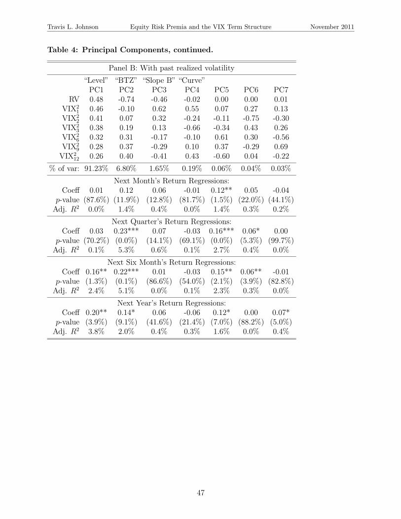
Travis L. Johnson Equity Risk Premia and the VIX Term Structure November 2011
Table 4: Principal Components, continued.
Panel B: With past realized volatility“Level” “BTZ” “Slope B” “Curve”PC1 PC2 PC3 PC4 PC5 PC6 PC7
RV 0.48 -0.74 -0.46 -0.02 0.00 0.00 0.01VIX2
1 0.46 -0.10 0.62 0.55 0.07 0.27 0.13VIX2
2 0.41 0.07 0.32 -0.24 -0.11 -0.75 -0.30VIX2
3 0.38 0.19 0.13 -0.66 -0.34 0.43 0.26VIX2
6 0.32 0.31 -0.17 -0.10 0.61 0.30 -0.56VIX2
9 0.28 0.37 -0.29 0.10 0.37 -0.29 0.69VIX2
12 0.26 0.40 -0.41 0.43 -0.60 0.04 -0.22% of var: 91.23% 6.80% 1.65% 0.19% 0.06% 0.04% 0.03%
Next Month’s Return Regressions:Coeff 0.01 0.12 0.06 -0.01 0.12** 0.05 -0.04
p-value (87.6%) (11.9%) (12.8%) (81.7%) (1.5%) (22.0%) (44.1%)Adj. R2 0.0% 1.4% 0.4% 0.0% 1.4% 0.3% 0.2%
Next Quarter’s Return Regressions:Coeff 0.03 0.23*** 0.07 -0.03 0.16*** 0.06* 0.00
p-value (70.2%) (0.0%) (14.1%) (69.1%) (0.0%) (5.3%) (99.7%)Adj. R2 0.1% 5.3% 0.6% 0.1% 2.7% 0.4% 0.0%
Next Six Month’s Return Regressions:Coeff 0.16** 0.22*** 0.01 -0.03 0.15** 0.06** -0.01
p-value (1.3%) (0.1%) (86.6%) (54.0%) (2.1%) (3.9%) (82.8%)Adj. R2 2.4% 5.1% 0.0% 0.1% 2.3% 0.3% 0.0%
Next Year’s Return Regressions:Coeff 0.20** 0.14* 0.06 -0.06 0.12* 0.00 0.07*
p-value (3.9%) (9.1%) (41.6%) (21.4%) (7.0%) (88.2%) (5.0%)Adj. R2 3.8% 2.0% 0.4% 0.3% 1.6% 0.0% 0.4%
47
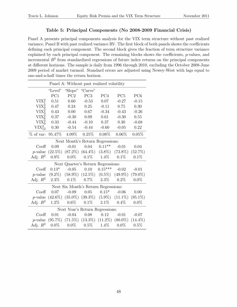
Travis L. Johnson Equity Risk Premia and the VIX Term Structure November 2011
Table 5: Principal Components (No 2008-2009 Financial Crisis)
Panel A presents principal components analysis for the VIX term structure without past realizedvariance, Panel B with past realized variance RV. The first block of both panels shows the coefficientsdefining each principal component. The second block gives the fraction of term structure varianceexplained by each principal component. The remaining blocks shows the coefficients, p-values, andincremental R2 from standardized regressions of future index returns on the principal componentsat different horizons. The sample is daily from 1996 through 2010, excluding the October 2008-June2009 period of market turmoil. Standard errors are adjusted using Newey-West with lags equal toone-and-a-half times the return horizon.
Panel A: Without past realized volatility
“Level” “Slope” “Curve”PC1 PC2 PC3 PC4 PC5 PC6
VIX21 0.51 0.60 -0.53 0.07 -0.27 -0.15
VIX22 0.47 0.24 0.25 -0.11 0.75 0.30
VIX23 0.43 0.00 0.67 -0.34 -0.43 -0.26
VIX26 0.37 -0.30 0.09 0.61 -0.30 0.55
VIX29 0.33 -0.44 -0.10 0.37 0.30 -0.68
VIX212 0.30 -0.54 -0.44 -0.60 -0.05 0.22
% of var: 95.47% 4.09% 0.25% 0.08% 0.06% 0.05%
Next Month’s Return Regressions:Coeff 0.09 -0.01 0.04 0.11** -0.01 0.04
p-value (22.5%) (87.2%) (64.4%) (3.8%) (73.8%) (52.7%)Adj. R2 0.9% 0.0% 0.1% 1.4% 0.1% 0.1%
Next Quarter’s Return Regressions:Coeff 0.13* -0.05 0.10 0.15*** -0.02 -0.01
p-value (9.2%) (58.9%) (12.5%) (0.5%) (49.9%) (79.0%)Adj. R2 2.3% 0.1% 0.7% 2.3% 0.2% 0.0%
Next Six Month’s Return Regressions:Coeff 0.07 -0.09 0.05 0.15* -0.06 0.00
p-value (42.6%) (35.0%) (39.3%) (5.9%) (11.1%) (95.1%)Adj. R2 1.2% 0.6% 0.1% 2.1% 0.4% 0.0%
Next Year’s Return Regressions:Coeff 0.01 -0.04 0.08 0.12 -0.01 -0.07
p-value (95.7%) (71.5%) (13.3%) (11.2%) (80.0%) (14.4%)Adj. R2 0.0% 0.0% 0.5% 1.4% 0.0% 0.5%
48
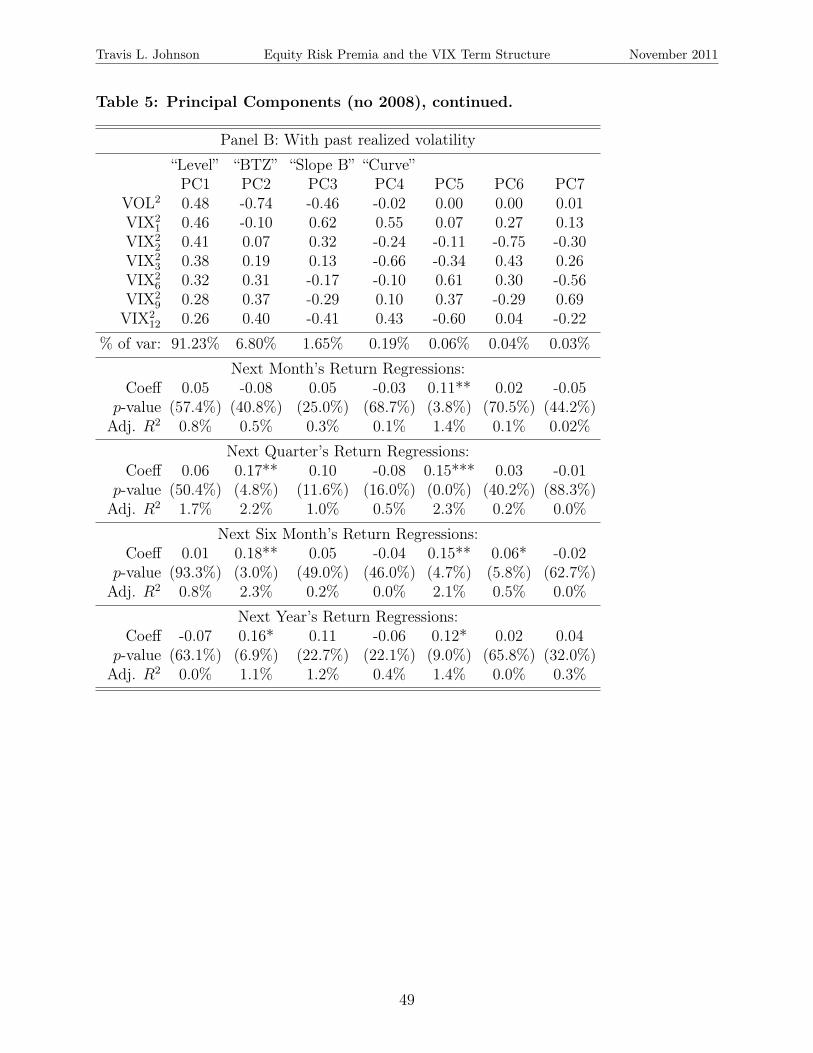
Travis L. Johnson Equity Risk Premia and the VIX Term Structure November 2011
Table 5: Principal Components (no 2008), continued.
Panel B: With past realized volatility“Level” “BTZ” “Slope B” “Curve”PC1 PC2 PC3 PC4 PC5 PC6 PC7
VOL2 0.48 -0.74 -0.46 -0.02 0.00 0.00 0.01VIX2
1 0.46 -0.10 0.62 0.55 0.07 0.27 0.13VIX2
2 0.41 0.07 0.32 -0.24 -0.11 -0.75 -0.30VIX2
3 0.38 0.19 0.13 -0.66 -0.34 0.43 0.26VIX2
6 0.32 0.31 -0.17 -0.10 0.61 0.30 -0.56VIX2
9 0.28 0.37 -0.29 0.10 0.37 -0.29 0.69VIX2
12 0.26 0.40 -0.41 0.43 -0.60 0.04 -0.22% of var: 91.23% 6.80% 1.65% 0.19% 0.06% 0.04% 0.03%
Next Month’s Return Regressions:Coeff 0.05 -0.08 0.05 -0.03 0.11** 0.02 -0.05
p-value (57.4%) (40.8%) (25.0%) (68.7%) (3.8%) (70.5%) (44.2%)Adj. R2 0.8% 0.5% 0.3% 0.1% 1.4% 0.1% 0.02%
Next Quarter’s Return Regressions:Coeff 0.06 0.17** 0.10 -0.08 0.15*** 0.03 -0.01
p-value (50.4%) (4.8%) (11.6%) (16.0%) (0.0%) (40.2%) (88.3%)Adj. R2 1.7% 2.2% 1.0% 0.5% 2.3% 0.2% 0.0%
Next Six Month’s Return Regressions:Coeff 0.01 0.18** 0.05 -0.04 0.15** 0.06* -0.02
p-value (93.3%) (3.0%) (49.0%) (46.0%) (4.7%) (5.8%) (62.7%)Adj. R2 0.8% 2.3% 0.2% 0.0% 2.1% 0.5% 0.0%
Next Year’s Return Regressions:Coeff -0.07 0.16* 0.11 -0.06 0.12* 0.02 0.04
p-value (63.1%) (6.9%) (22.7%) (22.1%) (9.0%) (65.8%) (32.0%)Adj. R2 0.0% 1.1% 1.2% 0.4% 1.4% 0.0% 0.3%
49