ER

DC

/GS

L T

R-0

9-9

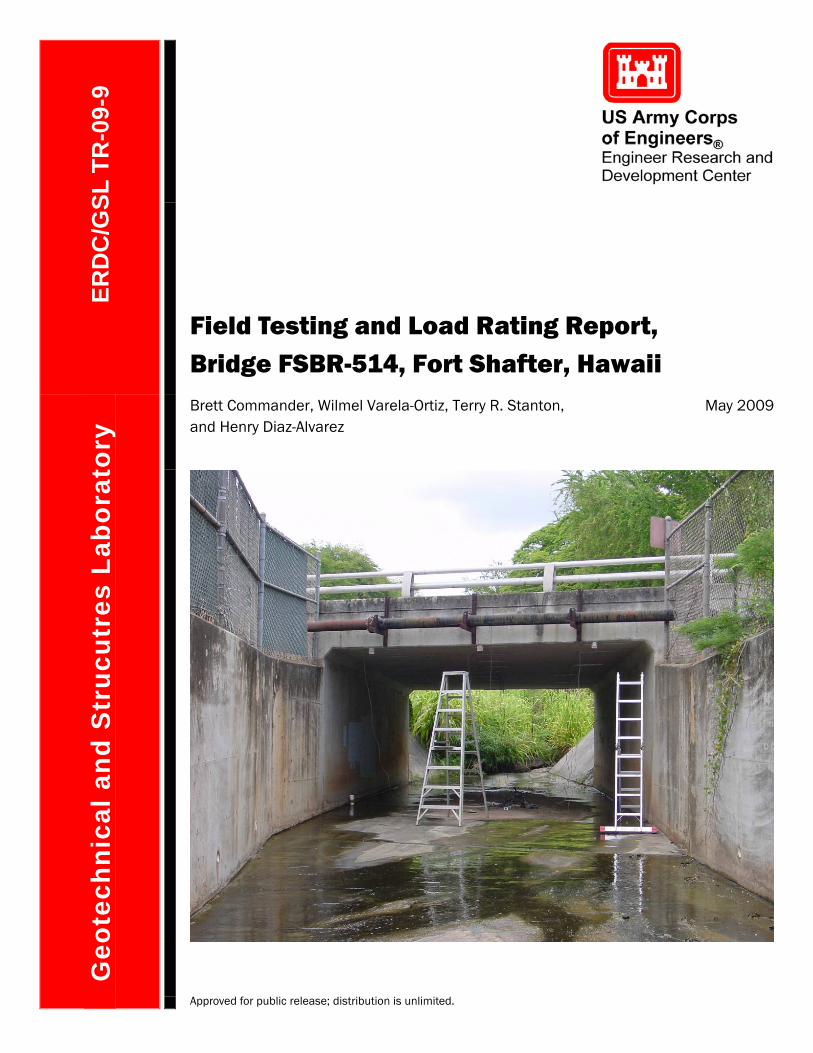
Field Testing and Load Rating Report,

Bridge FSBR-514, Fort Shafter, Hawaii

Brett Commander, Wilmel Varela-Ortiz, Terry R. Stanton, and Henry Diaz-Alvarez

May 2009

Ge

ote

ch

nic

al

an

d S

tru

cu

tre

s L

ab

ora

tory

Approved for public release; distribution is unlimited.

ERDC/GSL TR-09-9 May 2009

Field Testing and Load Rating Report,

Bridge FSBR-514, Fort Shafter, Hawaii

Brett Commander

Bridge Diagnostics, Inc. 1965 57th Court North, Suite 106 Boulder, CO 80301

Wilmel Varela-Ortiz, Terry R. Stanton, and Henry Diaz-Alvarez

Geotechnical and Structures Laboratory U.S. Army Engineer Research and Development Center 3909 Halls Ferry Road Vicksburg, MS 39180-6199

Final report

Approved for public release; distribution is unlimited.

Prepared for Headquarters, Installation Management Command (IMCOM) Arlington, VA 22202

ERDC/GSL TR-09-9 ii

Abstract: Bridge Diagnostics was contracted by the U.S. Army Corps of Engineers to perform live-load testing and load rating on Bridge FSBR-514 on Walker Road over Kahauiki Stream, Fort Shafter, Hawaii, in conjunc-tion with three other structures—Bridge FSBR-201, FSBR-1608, and ERBR-9. A primary goal of the live-load testing was to determine the rela-tive effects of different military load configurations. A second goal was to use the measured load responses to verify and calibrate a finite element model of the structure.

The load test results indicated that the culvert was relatively stiff and did a good job of distributing load. Load ratings resulting from the field-verified model indicated that all examined load configurations could cross the bridge within inventory (design) limits.

Load ratings were computed in accordance with the American Association of State Highway and Transportation Officials’ AASHTO LRFD bridge design specifications (2004) and Manual for the condition evaluation and load and resistance factor rating of highway bridges (2003).

DESTROY THIS REPORT WHEN NO LONGER NEEDED. DO NOT RETURN IT TO THE ORIGINATOR.

DISCLAIMER: The contents of this report are not to be used for advertising, publication, or promotional purposes. Citation of trade names does not constitute an official endorsement or approval of the use of such commercial products. All product names and trademarks cited are the property of their respective owners. The findings of this report are not to be construed as an official Department of the Army position unless so designated by other authorized documents.

ERDC/GSL TR-09-9 iii

Contents

Figures and Tables..................................................................................................................................v

Preface....................................................................................................................................................vi

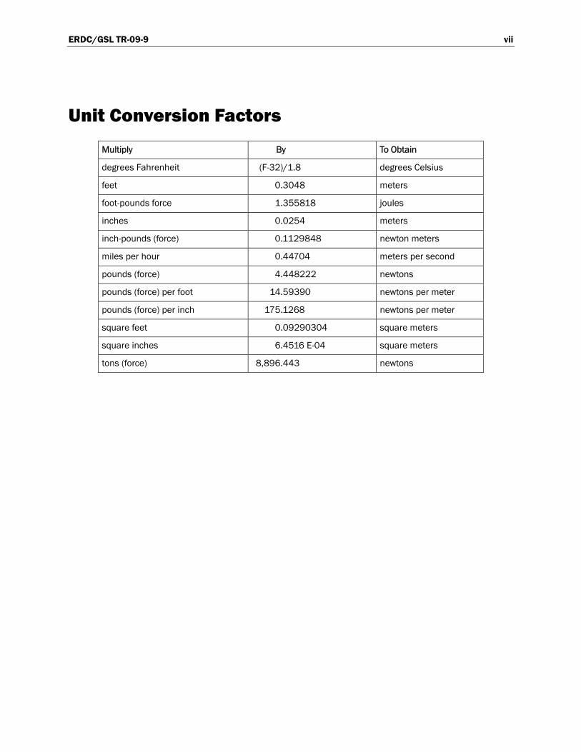
Unit Conversion Factors.......................................................................................................................vii

1 Introduction..................................................................................................................................... 1 Background .............................................................................................................................. 1 Results summary...................................................................................................................... 1 Additional information.............................................................................................................. 2

2 Structural Testing Information...................................................................................................... 3 Load test instrumentation ....................................................................................................... 3 GPR assessments .................................................................................................................... 6

3 Preliminary Investigation of Test Results.................................................................................... 9 General ..................................................................................................................................... 9 Preliminary data review observations ..................................................................................... 9

Reproducibility and linearity ........................................................................................................ 9 Distribution ................................................................................................................................... 9 End restraint...............................................................................................................................10 Response symmetry...................................................................................................................10 Unusual response ......................................................................................................................10

4 Modeling, Analysis, and Data Correlation.................................................................................14 Discussion ..............................................................................................................................14 Model calibration results .......................................................................................................15

Slab elastic modulus..................................................................................................................16 Support conditions.....................................................................................................................17

5 Load Rating Procedures and Results.........................................................................................18

6 Conclusions and Recommendations .........................................................................................22

References............................................................................................................................................23

Appendix A: Measured and Computed Strain Comparisons...........................................................24

Appendix B: Field Notes (scanned)....................................................................................................35

Appendix C: Field Testing Procedures...............................................................................................37

Appendix D: Specifications – BDI Strain Transducers.....................................................................44

Appendix E: Specifications – BDI Structural Testing System.........................................................45

ERDC/GSL TR-09-9 iv

Appendix F: Specifications – BDI AutoClicker .................................................................................47

Appendix G: Modeling and Analysis—The Integrated Approach.....................................................48

Appendix H: Load Rating Procedures................................................................................................56

Report Documentation Page

ERDC/GSL TR-09-9 v

Figures and Tables

Figures

Figure 1. Instrumentation plan. ................................................................................................................ 3 Figure 2. Cross-sectional views................................................................................................................. 5 Figure 3. Tandem rear axle dump truck footprint. .................................................................................. 5 Figure 4. Migration processing procedure to achieve final results for FSBR-514................................ 7 Figure 5. Three-dimensional representation of internal reinforcement................................................ 8 Figure 6. Three-dimensional representation of internal reinforcement, gathered from GPR evaluations................................................................................................................ 8 Figure 7. Reproducibility and linearity of test results. ...........................................................................11 Figure 8. Lateral distribution along midspan of slab. ...........................................................................11 Figure 9. Midspan strain history from east parapet. ............................................................................12 Figure 10. Negative strains 30 in. from abutment wall—indicating end restraint..............................12 Figure 11. Response symmetry. .............................................................................................................13 Figure 12. Crack running parallel to gage 8267. ..................................................................................13 Figure 13. Finite element model of superstructure. ............................................................................. 14

Tables

Table 1. Critical load rating factors (RF) and weights.............................................................................. 1 Table 2. Structure description and testing notes. ................................................................................... 4 Table 3. Testing vehicle information (tandem rear axle dump truck).1 ................................................. 5 Table 4. Analysis and model details. ...................................................................................................... 14 Table 5. Model accuracy and parameter values. .................................................................................. 16 Table 6. Load and resistance factors. ....................................................................................................19 Table 7. Material properties.....................................................................................................................19 Table 8. Section moment capacities. .....................................................................................................19 Table 9. Rating factor calculation for HS-20..........................................................................................20 Table 10. Rating factor calculation for MLC70 (wheeled). ...................................................................20 Table 11. Load rating factors and critical moment and shear values................................................. 21

ERDC/GSL TR-09-9 vi

Preface

This report describes the load testing process and analytical results con-ducted for Bridge FSBR-514 at Fort Shafter, Hawaii. The load test was one of four that were performed in July 2006 to obtain more accurate bridge load ratings with respect to civilian and military load configurations. This project was arranged and supervised by Wilmel Varela-Ortiz of the U.S. Army Engineer Research and Development Center (ERDC).

The work was performed by Bridge Diagnostics, Inc. (BDI), under U.S. Army Corps of Engineers contract number W912HZ-07-C-0045. This report was prepared by Brett Commander of BDI, along with Varela-Ortiz, Terry R. Stanton, and Henry Diaz-Alvarez of the ERDC Geotechnical and Structures Laboratory (GSL), Structural Engineering Branch (StEB). Technical review of the document was performed by Carmen Y. Lugo and Sharon Garner, StEB. Special recognition is given to the Directorate of Public Works at Fort Shafter.

The Army Bridge Inspection Program is sponsored by the Army Transportation Infrastructure Program (ATIP) of the Headquarters, Installation Management Command (IMCOM), Arlington, VA. The IMCOM provided funding for this investigation. Questions should be directed to Ali A. Achmar, IMCOM ATIP Program Manager, telephone: (210) 295-2038.

This publication was prepared under the overall project supervision of James S. Shore, Chief, StEB; Dr. Robert L. Hall, Chief, Geosciences and Structures Division; Dr. William P. Grogan, Deputy Director, GSL; and Dr. David W. Pittman, Director, GSL.

COL Gary E. Johnston was Commander and Executive Director of ERDC. Dr. James R. Houston was Director.

ERDC/GSL TR-09-9 vii

Unit Conversion Factors

Multiply By To Obtain

degrees Fahrenheit (F-32)/1.8 degrees Celsius

feet 0.3048 meters

foot-pounds force 1.355818 joules

inches 0.0254 meters

inch-pounds (force) 0.1129848 newton meters

miles per hour 0.44704 meters per second

pounds (force) 4.448222 newtons

pounds (force) per foot 14.59390 newtons per meter

pounds (force) per inch 175.1268 newtons per meter

square feet 0.09290304 square meters

square inches 6.4516 E-04 square meters

tons (force) 8,896.443 newtons

ERDC/GSL TR-09-9 1

1 Introduction

Background

The Bridge Diagnostics, Inc. (BDI), Structural Testing System (STS) was used for measuring strains at 24 locations on the superstructure of Bridge FSBR-514, Fort Shafter, Hawaii, while it was subjected to a moving truck load. The response data were then used to “calibrate” a finite element model of the structure, which was in turn used to develop load ratings for specified American Association of State Highway and Transportation Offi-cials (AASHTO) vehicles and selected military vehicles using the Load and Resistance Factor Rating (LRFR) approach.

No design or as-built plans were available for this structure. Therefore, U.S. Army Engineer Research and Development Center (ERDC) personnel used ground penetrating radar (GPR) to locate and size reinforcement steel in the slab. Steel information was provided only for the midspan loca-tion on the slab; therefore, load ratings will be limited to positive moment capacities at midspan.

Results summary

Based on the calibrated model and information provided by ERDC, the critical components of the structure were determined to be the interior midspan deck elements measuring 15.5 in. deep. Table 1 summarizes the critical load rating factors and load limits for the standard AASHTO rating vehicles and selected military vehicles.

Table 1. Critical load rating factors (RF) and weights.

LRFR - Inventory LRFR - Operating Truck 1

Rating Factor Tons Rating Factor Tons

HS-20 2.19 79 2.84 102

Type 3 2.88 72 3.73 93

Type 3S2 3.17 114 4.11 148

Type 3-3 3.52 141 4.56 183

LAVIII-Stryker2 2.11 43 2.74 56

PLS 2.70 185 3.50 240

ERDC/GSL TR-09-9 2

LRFR - Inventory LRFR - Operating Truck 1

Rating Factor Tons Rating Factor Tons

HETS2 2.49 286 3.23 371

MLC60 (tracked) 2 2.00 120 2.59 156

MLC60 (wheeled) 2 2.12 148 2.75 192

MLC70 (tracked) 2 1.84 129 2.39 167

MLC70 (wheeled) 2 1.83 147 2.37 191

1 Location = midspan of deck slab. 2 Single-lane loading.

The results obtained from the load ratings established that the real capac-ity of the bridge is considerably higher than the one from the previous load rating analysis, which was based on a slab strip methodology. The primary sources of increased stiffness and capacity came from the relatively thick deck compared to the span length and the relatively large quantity of longitudinal steel. Therefore, it is likely this bridge was originally designed for military moving loads. Since no top steel information was available to compute negative moment capacities at the abutments, it was conserva-tively assumed that the culvert top would fail due to negative moment at the supports prior to the development of the maximum midspan moment. The rating model was adjusted to accommodate the formation of a hinge at the end of the slab. This was done by removing the high degree of slab end-restraint provided by the abutment walls. In this case, the load rating was still controlled by the midspan positive moment, but the assumption was that the negative moment hinges would fail first. This level of conservatism was necessary due to the lack of steel information. Even so, the bridge has an exceptionally high load rating.

Additional information

Descriptions of the test procedures and equipment specifications are pre-sented in the appendixes to this report: A, Measured and computed strain comparisons; B, Field notes; C, Field testing procedures; D, Specifica-tions–BDI strain transducers; E, Specifications–BDI Structural Testing System; F, Specifications–BDI Autoclicker; G, Modeling and analysis–integrated approach; and H, load rating procedures.

ERDC/GSL TR-09-9 3

2 Structural Testing Information

Load test instrumentation

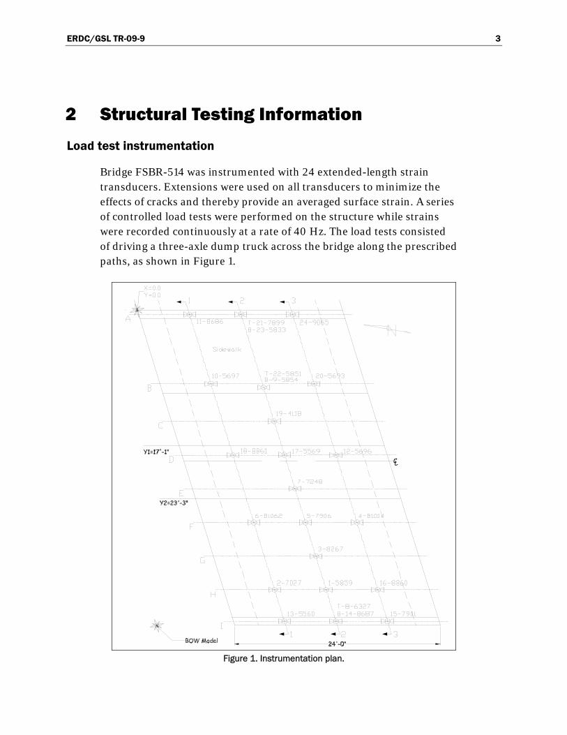
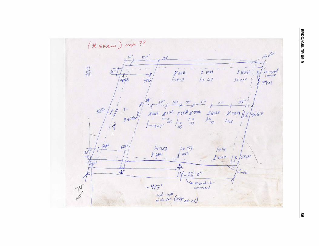
Bridge FSBR-514 was instrumented with 24 extended-length strain transducers. Extensions were used on all transducers to minimize the effects of cracks and thereby provide an averaged surface strain. A series of controlled load tests were performed on the structure while strains were recorded continuously at a rate of 40 Hz. The load tests consisted of driving a three-axle dump truck across the bridge along the prescribed paths, as shown in Figure 1.

Figure 1. Instrumentation plan.

ERDC/GSL TR-09-9 4

Paths shown in Figure 1 represent the position of the driver’s side front wheel. The longitudinal position of the truck was monitored remotely and recorded along with the strain data. Information specific to this load test is provided in Table 2 and Table 3, and in the field notes presented as Appendix B. Cross-sectional views of the test path (Figure 2) and the testing vehicle’s footprint (Figure 3) are also illustrated.

Table 2. Structure description and testing notes.

Item Description

Structure name FSBR514

Date of construction 1978

BDI project number 070603

Testing date August 3, 2006

Client’s structure ID# FSBR514

Location/route Walker Drive over Kahauiki Stream, Hawaii

Structure type Reinforced concrete (RC) box culvert

Total number of spans 1

Span length(s) 24 ft

Skew 17

Structure/roadway width 38 ft, 6 in. /26 ft, 6 in.

Deck type RC

Other structure info N/A

Spans tested 1

Test reference location (X = 0,Y = 0) Northeast corner, on top of parapet

Test vehicle direction Southbound

Test beginning point -10 ft - ½ wheel revolution = -15.11 ft

Lateral load position(s) 17 ft, 1 in. /23 ft, 3 in.

Number/type of sensors 24 strain transducers

STS sample rate 40 Hz

Number of test vehicles 1

Structure access type Ladder

Structure access provided by U.S. Army Corps of Engineers

Traffic control provided by U.S. Army Corps of Engineers

Total field testing time 8 hr

Field notes See Appendix B

Additional nondestructive testing info GPR used to locate and identify reinforcement slab. Longitudinal steel and transverse steel provided by ERDC.

Visual condition Fair condition; significant cracking

ERDC/GSL TR-09-9 5

Table 3. Testing vehicle information (tandem rear axle dump truck).1

Parameter Value

Gross vehicle weight (GVW) 39,100 lb

Wheel rollout, five revs 51.1 ft

No. crawl-speed passes 5 passes – 2 paths

No. high-speed passes/speed 0

1 See Figure 3.

Figure 2. Cross-sectional views.

Figure 3. Tandem rear axle dump truck footprint.

ERDC/GSL TR-09-9 6

GPR assessments

For these investigations, since no plans were available for the tested struc-tures, GPR was employed to determine the size, location, and amount of reinforcing steel. The 1600-MHz (GSSI Model 5100) antenna was used since it possesses the best combination of depth and resolution for the inspection of structural concrete. Once the reinforcing steel was located, small holes were drilled into the concrete to verify the size of the reinforc-ing bars. All holes were then filled with a two-part concrete-epoxy to pre-vent any deterioration of the reinforcing steel. The structural members were then carefully measured so that, when combined with the GPR infor-mation, “as-built” plans could be developed. Note that no attempt was made to evaluate negative moment reinforcement at the abutments during this study.

Figure 4 shows the migration processing procedures used to achieve the final results for the evaluated bridge. This procedure reduces or eliminates hyperbolic diffraction patterns in the data. It basically takes out the tails of the hyperbolas to more accurately represent the location of the target. This process also offers a simple and accurate way of calculating, from the shape of the hyperbolas, the dielectric of the material in which the target located. Note that in Figure 4b each hyperbola has been collapsed into dots, which means that the dielectric of the material is appropriate. After the migration process has been completed, the final data show the corre-spondent location and spacing of the reinforcing steel in the slab (Figure 4c).

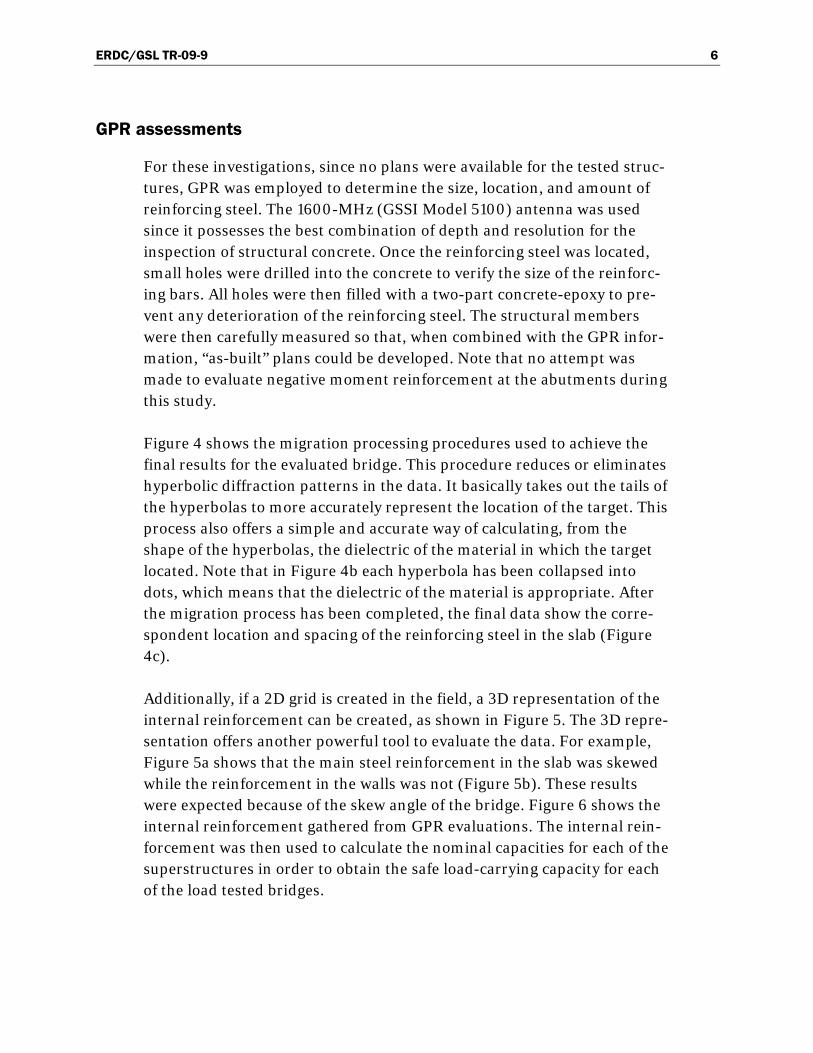
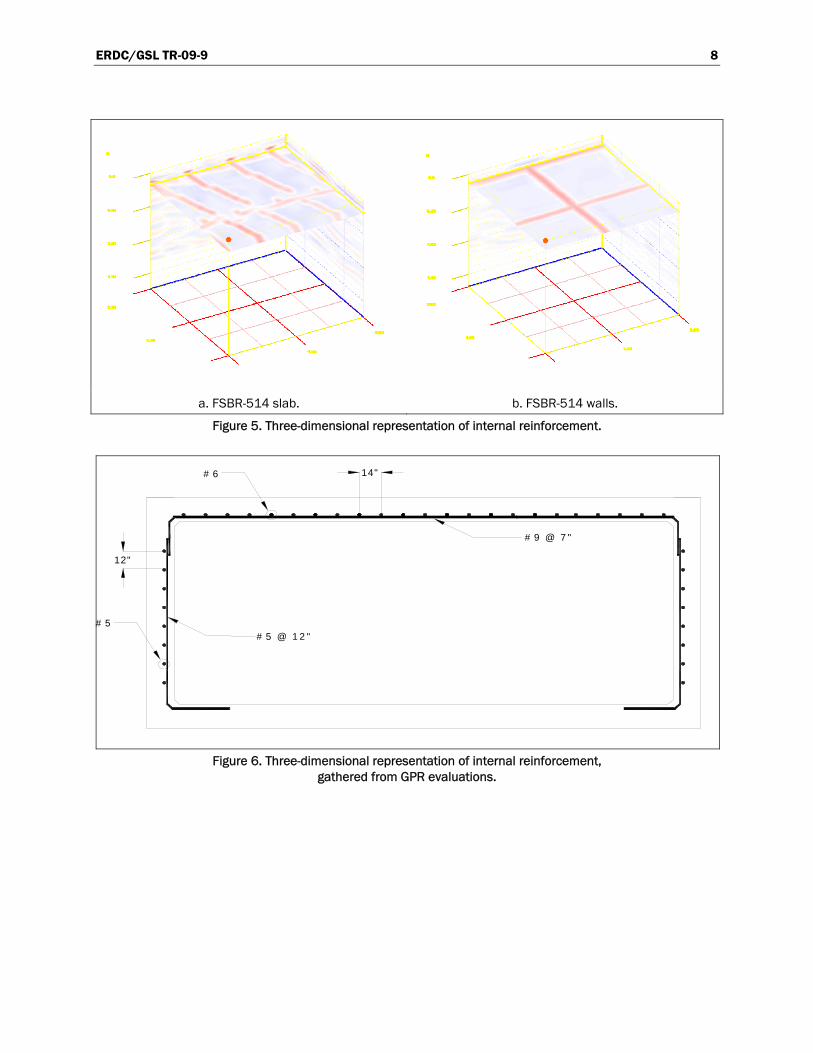
Additionally, if a 2D grid is created in the field, a 3D representation of the internal reinforcement can be created, as shown in Figure 5. The 3D repre-sentation offers another powerful tool to evaluate the data. For example, Figure 5a shows that the main steel reinforcement in the slab was skewed while the reinforcement in the walls was not (Figure 5b). These results were expected because of the skew angle of the bridge. Figure 6 shows the internal reinforcement gathered from GPR evaluations. The internal rein-forcement was then used to calculate the nominal capacities for each of the superstructures in order to obtain the safe load-carrying capacity for each of the load tested bridges.

ERDC/GSL TR-09-9 7

a. Raw data.

b. Migrated data.

c. Final results.

Concrete Surface

Reinforcing Steel

Collapsed Hyperbolas

Concrete Surface

Reinforcing Steel

Figure 4. Migration processing procedure to achieve final results for FSBR-514.

ERDC/GSL TR-09-9 8

a. FSBR-514 slab. b. FSBR-514 walls.

Figure 5. Three-dimensional representation of internal reinforcement.

#9 @ 7"

14"#6

#5 @ 12"

12"

#5

Figure 6. Three-dimensional representation of internal reinforcement,

gathered from GPR evaluations.

ERDC/GSL TR-09-9 9

3 Preliminary Investigation of Test Results

General

All of the field data were first examined graphically to determine the qual-ity and to provide a qualitative assessment of the structure’s live-load response. Some of the indicators of data quality included reproducibility between identical truck crossings, elastic behavior (strains returning to zero after truck crossing), and any unusual-shaped responses that might indicate nonlinear behavior or possible gage malfunctions.

In addition to providing a data “quality check,” the information obtained during the preliminary investigation was used to determine appropriate modeling procedures and helped to establish the direction the analysis should take. Several representative response histories are provided in Appendix A.

Preliminary data review observations

Reproducibility and linearity

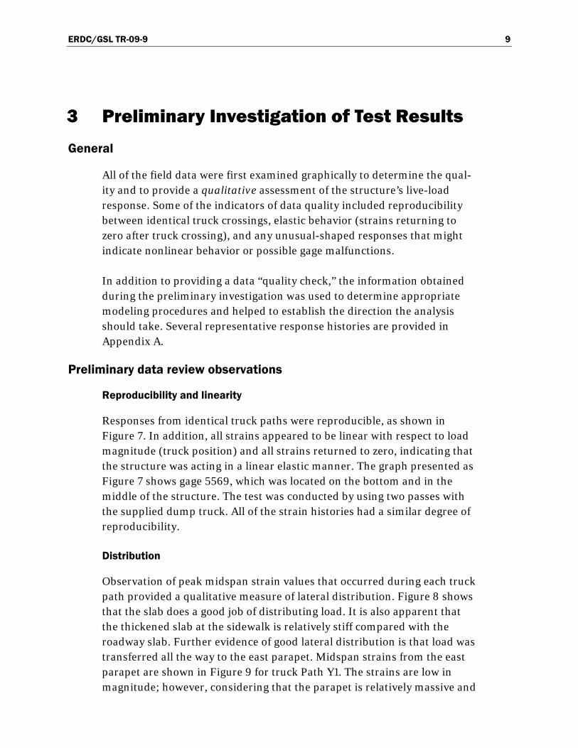
Responses from identical truck paths were reproducible, as shown in Figure 7. In addition, all strains appeared to be linear with respect to load magnitude (truck position) and all strains returned to zero, indicating that the structure was acting in a linear elastic manner. The graph presented as Figure 7 shows gage 5569, which was located on the bottom and in the middle of the structure. The test was conducted by using two passes with the supplied dump truck. All of the strain histories had a similar degree of reproducibility.

Distribution

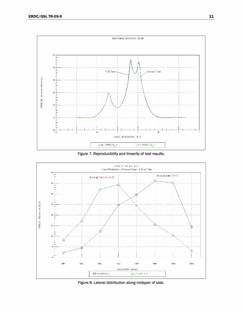
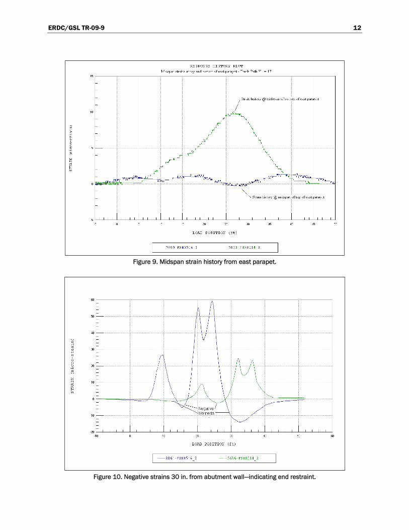
Observation of peak midspan strain values that occurred during each truck path provided a qualitative measure of lateral distribution. Figure 8 shows that the slab does a good job of distributing load. It is also apparent that the thickened slab at the sidewalk is relatively stiff compared with the roadway slab. Further evidence of good lateral distribution is that load was transferred all the way to the east parapet. Midspan strains from the east parapet are shown in Figure 9 for truck Path Y1. The strains are low in magnitude; however, considering that the parapet is relatively massive and

ERDC/GSL TR-09-9 10

stiff, it carries a significant amount of load. This was significant because the parapet was approximately 12 ft from the nearest truck wheel line.

End restraint

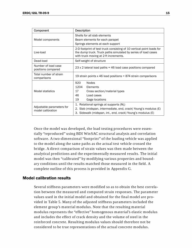
Negative strain values occurred near the ends of the culvert top. Figure 10 represents the strain value in line D. This type of response was found to be typical, which suggests a high degree of fixed end-restraint in the struc-ture. This was confirmed by field operations that found the culvert walls to be 2 ft, 10 in. thick.

Response symmetry

Comparison of strain magnitudes from the ends of the culvert top indi-cated a lack of symmetry. This observation is not unexpected, because of the skew, asymmetric loading, and thickened slab along the east side of the bridge. Figure 11 shows the relative magnitudes of the midspan beam strains due to the east and west truck paths.

Unusual response

Gage 8267 showed an exceptionally small strain response for all load posi-tions. When compared with adjacent gage locations, the strain values were approximately one-fourth the typical strain magnitudes. The most likely reason for the low responses was that the strains were heavily influenced by local cracks. Extensions were used to average the strain over a distance of 12 in. and thereby minimize the effects of cracks. In this case, a signifi-cant longitudinal crack ran parallel to the gage. The exact mechanism for the low strains on Gage 8267 is not known, but it was determined the responses were strictly local and not due to any primary structural response. Figure 12 shows Gage 8267 and its relative location next to the longitudinal crack. As a result of unusually low response, this gage and the gages at the sidewalk parapet were not used in the finite element model calibration or load ratings.

ERDC/GSL TR-09-9 11

Figure 7. Reproducibility and linearity of test results.

Figure 8. Lateral distribution along midspan of slab.

ERDC/GSL TR-09-9 12

Figure 9. Midspan strain history from east parapet.

Figure 10. Negative strains 30 in. from abutment wall—indicating end restraint.

ERDC/GSL TR-09-9 13

Figure 11. Response symmetry.

Figure 12. Crack running parallel to gage 8267.

ERDC/GSL TR-09-9 14

4 Modeling, Analysis, and Data Correlation

Discussion

Note that all of the information presented in Chapter 3 was determined by simply viewing the field data and was used to generate a representative finite element model, as shown in Figure 13. Details regarding the struc-ture model and analysis procedures are provided in Table 4.

Figure 13. Finite element model of superstructure.

Table 4. Analysis and model details.

Component Description

Analysis type Linear-elastic finite element – stiffness method

Model geometry Planar-grid composed of shell elements, beam lines and springs

Nodal locations Nodes placed at all bearing locations Nodes at all four corners of each plate element

ERDC/GSL TR-09-9 15

Component Description

Model components Shells for all slab elements Beam elements for each parapet Springs elements at each support

Live-load 2-D footprint of test truck consisting of 10 vertical point loads for the dump truck. Truck paths simulated by series of load cases with truck moving at 2-ft increments.

Dead-load Self-weight of structure

Number of load case positions compared

23 x 2 lateral load paths = 46 load case positions compared

Total number of strain comparisons

19 strain points x 46 load positions = 874 strain comparisons

Model statistics

920 Nodes 1204 Elements 17 Cross section/material types 46 Load cases 19 Gage locations

Adjustable parameters for model calibration

1. Rotational springs at supports (My) 2. Slab (midspan, intermediate, end, crack) Young’s modulus (E) 3. Sidewalk (midspan, int., end, crack) Young’s modulus (E)

Once the model was developed, the load testing procedures were essen-tially “reproduced” using BDI WinSAC structural analysis and correlation software. A two-dimensional “footprint” of the loading vehicle was applied to the model along the same paths as the actual test vehicle crossed the bridge. A direct comparison of strain values was then made between the analytical predictions and the experimentally measured results. The initial model was then “calibrated” by modifying various properties and bound-ary conditions until the results matched those measured in the field. A complete outline of this process is provided in Appendix G.

Model calibration results

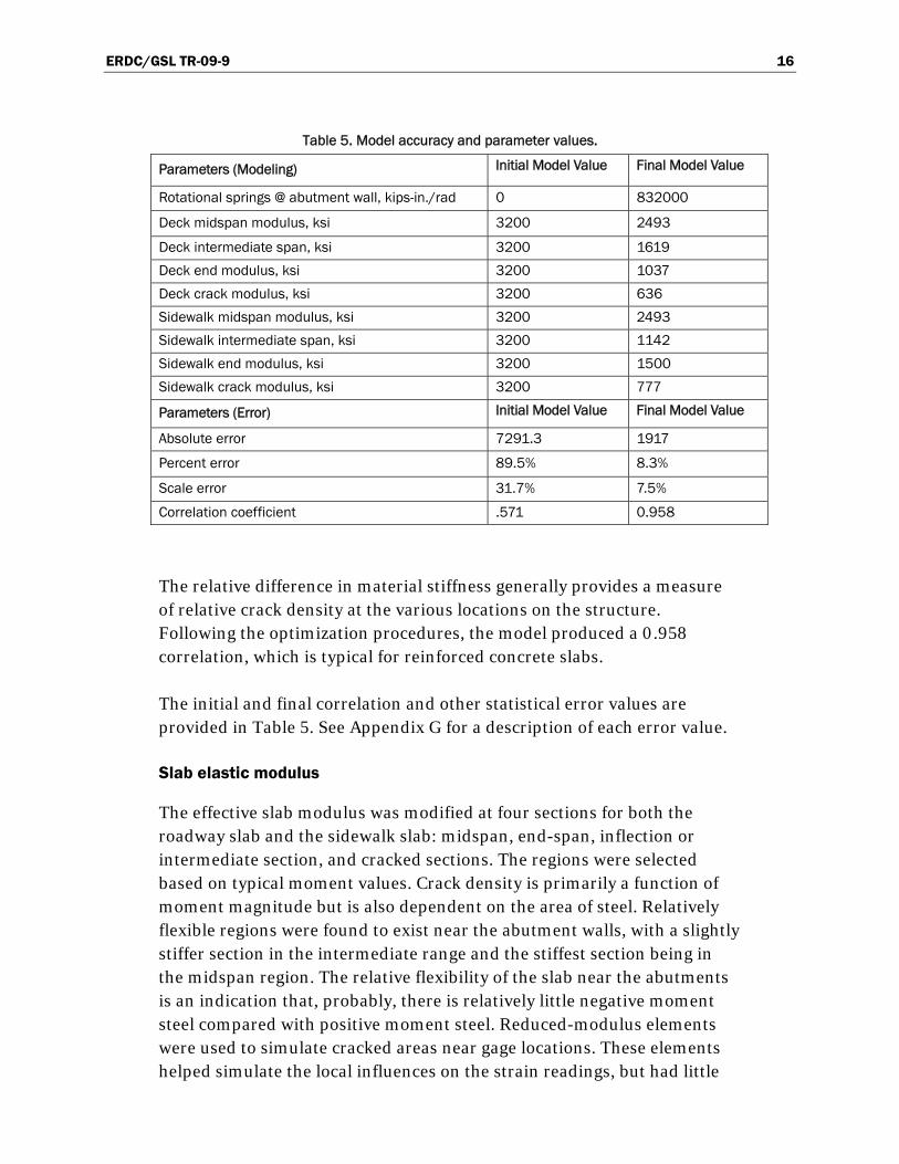
Several stiffness parameters were modified so as to obtain the best correla-tion between the measured and computed strain responses. The parameter values used in the initial model and obtained for the final model are pro-vided in Table 5. Many of the adjusted stiffness parameters included the element group’s material modulus. Note that the resulting material modulus represents the “effective” homogenous material’s elastic modulus and includes the effect of crack density and the volume of steel in the reinforced concrete. Resulting modulus values should therefore not be considered to be true representations of the actual concrete modulus.

ERDC/GSL TR-09-9 16

Table 5. Model accuracy and parameter values.

Parameters (Modeling) Initial Model Value Final Model Value

Rotational springs @ abutment wall, kips-in./rad 0 832000

Deck midspan modulus, ksi 3200 2493

Deck intermediate span, ksi 3200 1619

Deck end modulus, ksi 3200 1037

Deck crack modulus, ksi 3200 636

Sidewalk midspan modulus, ksi 3200 2493

Sidewalk intermediate span, ksi 3200 1142

Sidewalk end modulus, ksi 3200 1500

Sidewalk crack modulus, ksi 3200 777

Parameters (Error) Initial Model Value Final Model Value

Absolute error 7291.3 1917

Percent error 89.5% 8.3%

Scale error 31.7% 7.5%

Correlation coefficient .571 0.958

The relative difference in material stiffness generally provides a measure of relative crack density at the various locations on the structure. Following the optimization procedures, the model produced a 0.958 correlation, which is typical for reinforced concrete slabs.

The initial and final correlation and other statistical error values are provided in Table 5. See Appendix G for a description of each error value.

Slab elastic modulus

The effective slab modulus was modified at four sections for both the roadway slab and the sidewalk slab: midspan, end-span, inflection or intermediate section, and cracked sections. The regions were selected based on typical moment values. Crack density is primarily a function of moment magnitude but is also dependent on the area of steel. Relatively flexible regions were found to exist near the abutment walls, with a slightly stiffer section in the intermediate range and the stiffest section being in the midspan region. The relative flexibility of the slab near the abutments is an indication that, probably, there is relatively little negative moment steel compared with positive moment steel. Reduced-modulus elements were used to simulate cracked areas near gage locations. These elements helped simulate the local influences on the strain readings, but had little

ERDC/GSL TR-09-9 17

effect on the global load transfer. Cracked regions were approximately one quarter the stiffness of the midspan region.

Support conditions

Rotational-restraint springs were used to simulate the connection of the slab to the culvert walls. The resulting rotational stiffness indicated a high degree of restraint approaching fixed-end conditions. This result corre-sponded with the apparent 30-in.-wide culvert walls. The end-restraint had the effect of reducing midspan moment to approximately 85 percent of the midspan moment for a simply supported slab and generating significant negative moment at the culvert walls.

ERDC/GSL TR-09-9 18

5 Load Rating Procedures and Results

The goal of producing an accurate model was to predict the structure’s actual live load behavior when subjected to design or rating loads. This approach is essentially identical to standard load rating procedures, except that a “field verified” model was used to determine midspan moment instead of the AASHTO strip method typically used to analyze slabs. (Refer to Appendix H for a detailed outline of the load rating procedures.)

Once the finite element model was calibrated to field conditions, engineer-ing judgment was used to address any optimized parameters that could change with time, loading, or damage, or that could not be verified. How-ever, the amount of negative moment steel at the abutments was not defined; thus, the moment capacity of the slab ends could not be obtained. To ensure a conservative rating, it was assumed that the slab would fail in negative moment at the abutments prior to failing at midspan. This condi-tion was simulated by removing the end-restraints provided by the spring elements. The resulting load capacity was then controlled by the midspan moment after a hinge condition was induced at the culvert walls.

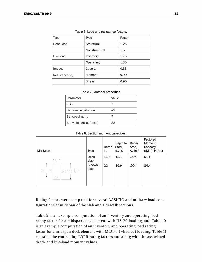
Capacities were calculated using the “AASHTO Manual for Condition Evaluation and Load and Resistance Factor Rating (LRFR) of Highway Bridges October 2003 Edition” and Equation 5.7.3.2.2-1 in “AASHTO LRFD Bridge Design Specifications, Third Edition, 2004.” Load rating fac-tors for the standard AASHTO vehicles were computed according to the LRFR rating method. Load and resistance factors used in the rating are listed in Table 6.

Table 7 contains the basic material properties and dimensions that were used for the member capacity calculations. Based on the available steel information, moment capacities were computed for the slab midspan and the sidewalk midspan. The size and spacing of all reinforcement steel was provided by the ERDC, based on GPR tests performed on the bridge. Table 8 outlines the calculated midspan moments for the slab sections.

Maximum live and dead-load shear and moment responses for each load configuration were obtained from the field-verified finite element model.

ERDC/GSL TR-09-9 19

Table 6. Load and resistance factors.

Type Type Factor

Dead load Structural 1.25

Nonstructural 1.5

Live load Inventory 1.75

Operating 1.35

Impact Case 1 0.33

Resistance (φ) Moment 0.90

Shear 0.90

Table 7. Material properties.

Parameter Value

b, in. 7

Bar size, longitudinal #9

Bar spacing, in. 7

Bar yield stress, fs (ksi) 33

Table 8. Section moment capacities.

Mid Span Type Depth in.

Depth to Steel, ds, in.

Rebar Area, As, in.2

Factored Moment Capacity, φMn (k-in./in.)

Deck slab Sidewalk slab

15.5 22

13.4 19.9

.994 .994

51.1 84.4

Rating factors were computed for several AASHTO and military load con-figurations at midspan of the slab and sidewalk sections.

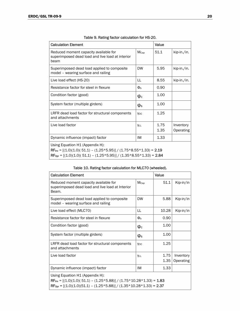
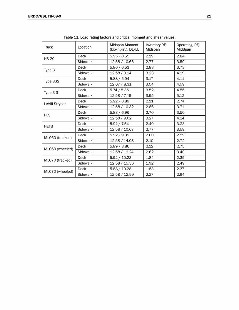
Table 9 is an example computation of an inventory and operating load rating factor for a midspan deck element with HS-20 loading, and Table 10 is an example computation of an inventory and operating load rating factor for a midspan deck element with MLC70 (wheeled) loading. Table 11 contains the controlling LRFR rating factors and along with the associated dead- and live-load moment values.

ERDC/GSL TR-09-9 20

Table 9. Rating factor calculation for HS-20.

Calculation Element Value

Reduced moment capacity available for superimposed dead load and live load at interior beam

MCap 51.1 kip-in./in.

Superimposed dead load applied to composite model – wearing surface and railing

DW 5.95 kip-in./in.

Live load effect (HS-20) LL 8.55 kip-in./in.

Resistance factor for steel in flexure Φb 0.90

Condition factor (good) φc 1.00

System factor (multiple girders) φs 1.00

LRFR dead load factor for structural components and attachments

γDC 1.25

Live load factor γLL 1.75 1.35

Inventory Operating

Dynamic influence (impact) factor IM 1.33

Using Equation H1 (Appendix H): RFInv = [(1.0)(1.0)( 51.1) – (1.25*5.95)] / (1.75*8.55*1.33) = 2.19 RFOpr = [(1.0)(1.0)( 51.1) – (1.25*5.95)] / (1.35*8.55*1.33) = 2.84

Table 10. Rating factor calculation for MLC70 (wheeled).

Calculation Element Value

Reduced moment capacity available for superimposed dead load and live load at Interior Beam.

MCap 51.1 Kip-in/in

Superimposed dead load applied to composite model – wearing surface and railing

DW 5.88 Kip-in/in

Live load effect (MLC70) LL 10.28 Kip-in/in

Resistance factor for steel in flexure Φb 0.90

Condition factor (good) φc 1.00

System factor (multiple girders) φs 1.00

LRFR dead load factor for structural components and attachments

γDC 1.25

Live load factor γLL 1.75 1.35

Inventory Operating

Dynamic influence (impact) factor IM 1.33

Using Equation H1 (Appendix H): RFInv = [(1.0)(1.0)( 51.1) – (1.25*5.88)] / (1.75*10.28*1.33) = 1.83 RFOpr = [(1.0)(1.0)(51.1) – (1.25*5.88)] / (1.35*10.28*1.33) = 2.37

ERDC/GSL TR-09-9 21

Table 11. Load rating factors and critical moment and shear values.

Truck Location Midspan Moment (kip-in./in.), DL/LL

Inventory RF, Midspan

Operating RF, MidSpan

Deck 5.95 / 8.55 2.19 2.84 HS-20

Sidewalk 12.58 / 10.66 2.77 3.59

Deck 5.86 / 6.53 2.88 3.73 Type 3

Sidewalk 12.58 / 9.14 3.23 4.19

Deck 5.88 / 5.94 3.17 4.11 Type 3S2

Sidewalk 12.67 / 8.31 3.54 4.59

Deck 5.74 / 5.35 3.52 4.56 Type 3-3

Sidewalk 12.58 / 7.46 3.95 5.12

Deck 5.92 / 8.89 2.11 2.74 LAVIII-Stryker

Sidewalk 12.58 / 10.32 2.86 3.71

Deck 5.88 / 6.96 2.70 3.50 PLS

Sidewalk 12.58 / 9.02 3.27 4.24

Deck 5.92 / 7.54 2.49 3.23 HETS

Sidewalk 12.58 / 10.67 2.77 3.59

Deck 5.92 / 9.39 2.00 2.59 MLC60 (tracked)

Sidewalk 12.58 / 14.03 2.10 2.72

Deck 5.89 / 8.86 2.12 2.75 MLC60 (wheeled)

Sidewalk 12.58 / 11.24 2.62 3.40

Deck 5.92 / 10.23 1.84 2.39 MLC70 (tracked)

Sidewalk 12.58 / 15.36 1.92 2.49

Deck 5.88 / 10.28 1.83 2.37 MLC70 (wheeled)

Sidewalk 12.58 / 12.99 2.27 2.94

ERDC/GSL TR-09-9 22

6 Conclusions and Recommendations

Conclusions made directly from the load test data were qualitative in nature and indicated that the structure was behaving normally for a rein-forced concrete box culvert. The structure appeared to be in fair condition with cracks in the longitudinal and transverse direction. All strain measurements indicated that the structure was behaving linearly with respect to load magnitude (truck position) and all responses were elastic. The measurements also indicated that there was significant lateral load transfer through the slab.

Results from the model calibration procedures showed that the slab was rigidly connected to the abutment walls. Relative slab stiffness throughout the structure indicated that the end regions of the slabs near the abutment wall are more flexible than the midspan regions. The increased flexibility is a measure of the crack density and was an indication that significant negative moment was developed along the slab-wall interface.

Prior to performing load rating, the model was adjusted to accommodate the formation of a hinge at each end of the slab. This was done because the negative moment capacity at the abutment was unknown. Therefore, a conservative assumption that the initial failure would occur at the negative moment region along the abutment walls was made. Hinges were simu-lated by eliminating the rotational restraint at slab ends, resulting in a simply supported slab. The structure’s load capacity was then based on the midspan moment capacity.

For the vehicles that were load rated, it can be concluded that the bridge will sustain the applied loads with a high degree of safety. All vehicles, including the tracked MLC60 and MLC70, can cross this structure within inventory limits.

The load rating factors and conclusions presented in this report are pro-vided as recommendations based on the structure’s response behavior and condition at the time of load testing. Any structural degradation must be considered in future load ratings. Note that no effort was made to assess the condition or capacity of the abutments.

ERDC/GSL TR-09-9 23

References

American Association of State Highway and Transportation Officials. 2004. AASHTO LRFD bridge design specifications. 3d ed. (includes 2005 and 2006 interims). Washington, DC.

_____. 2003. Manual for the condition evaluation and load and resistance factor Rating (LRFR) of highway bridges. Washington, DC.

Commander, B. 1989. An improved method of bridge evaluation: comparison of field test results with computer analysis. MS thesis, Univ. of Colorado, Boulder.

Gerstle, K. H., and M. H. Ackroyd. 1990. Behavior and design of flexibly connected building frames. Engineering Journal, AISC 27(1), 22–29.

Goble, G., J. Schulz, and B. Commander. 1992. Load prediction and structural response. Report FHWA DTFH61-88-C-00053. Boulder, CO: Univ. of Colorado.

Lichtenstein, A. G. 1993. Bridge rating through nondestructive load testing. Technical Report, National Cooperative Highway Research Program, Project 12-28(13)A. Washington, DC: Transportation Research Board.

Schulz, J. L. 1989. Development of a digital strain measurement system for highway bridge testing. MS thesis, Univ. of Colorado, Boulder.

_____. 1993. In search of better load ratings. Civil Engineering, ASCE 63(9):62–65.

ERDC/GSL TR-09-9 24

Appendix A: Measured and Computed Strain Comparisons

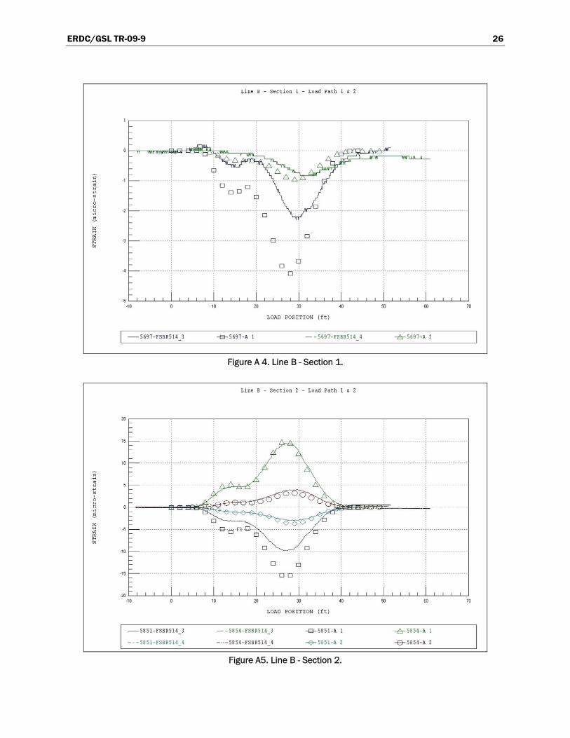
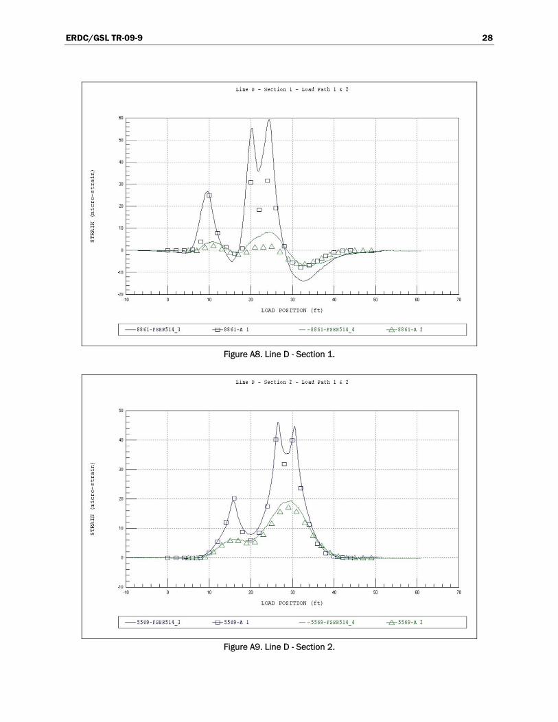
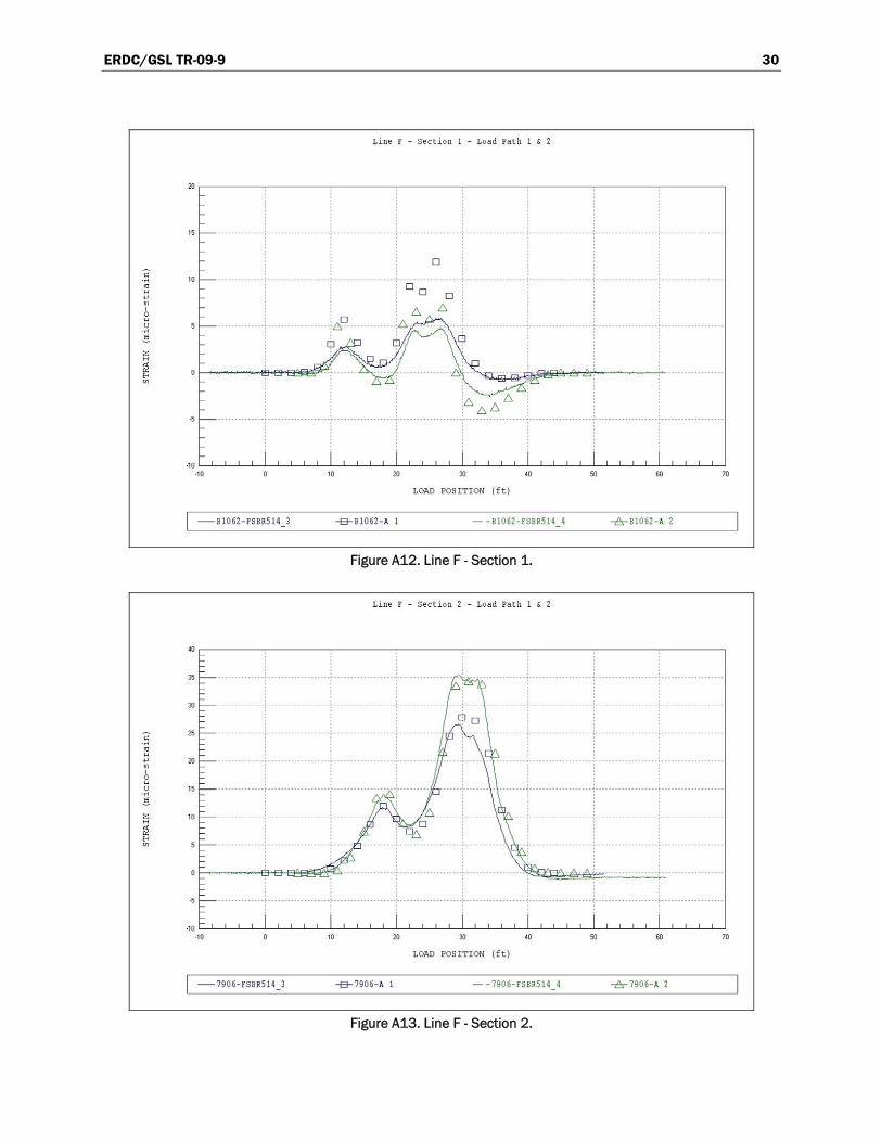
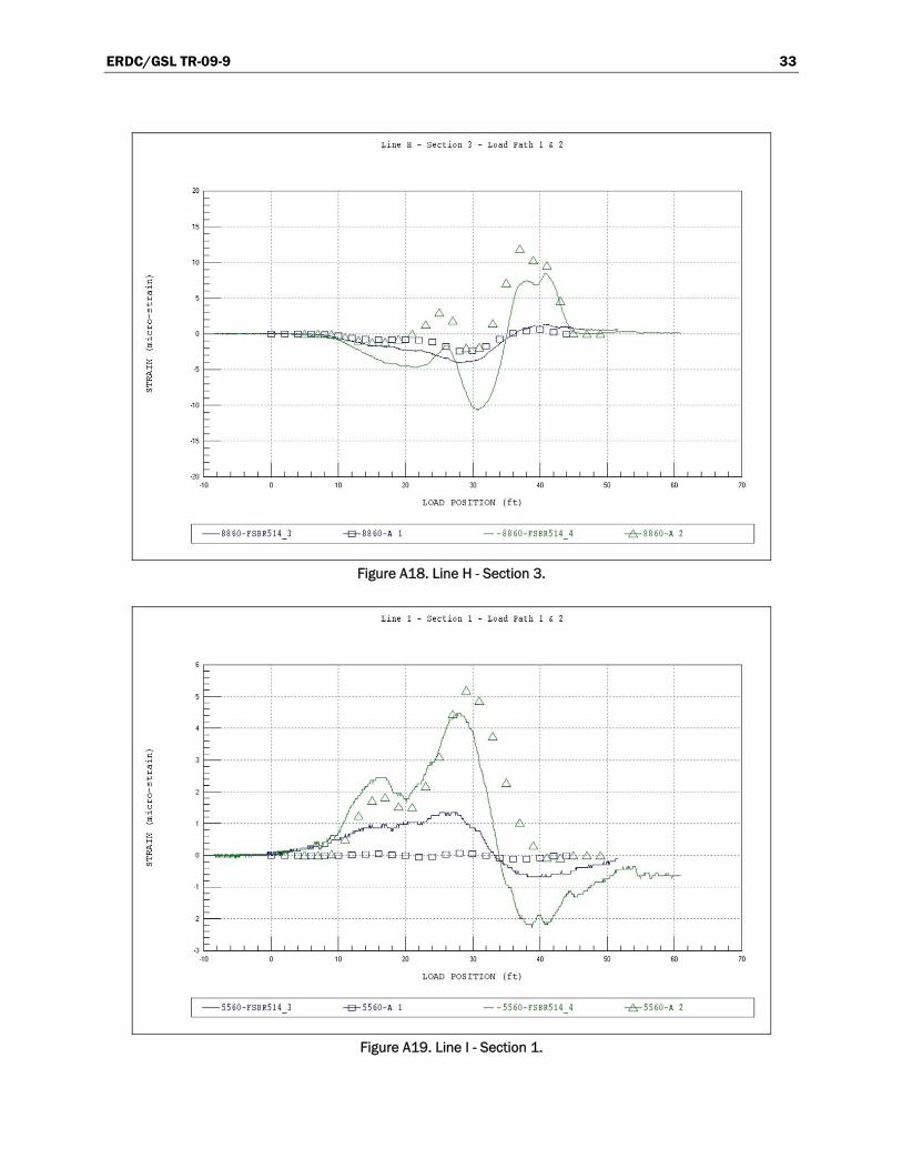
While statistical terms provide a means of evaluating the relative accuracy of various modeling procedures or help determine the improvement of a model during a calibration process, the best conceptual measure of a model’s accuracy is visual examination of the response histories. The graphs included as Figures A1–A21 present measured and computed strain histories from each truck path. In each graph, the continuous lines repre-sent the measured strain at the specified gage location as a function of truck position as it traveled across the bridge. Computed strains are shown as markers at discrete truck intervals.

Figure A1. Line A - Section 1 – gages not used.

ERDC/GSL TR-09-9 25

Figure A2. Line A - Section 2 – gages not used.

Figure A3. Line A - Section 3 – gages not used.

ERDC/GSL TR-09-9 26

Figure A 4. Line B - Section 1.

Figure A5. Line B - Section 2.

ERDC/GSL TR-09-9 27

Figure A6. Line B - Section 3.

Figure A7. Line C - Section 2.

ERDC/GSL TR-09-9 28

Figure A8. Line D - Section 1.

Figure A9. Line D - Section 2.

ERDC/GSL TR-09-9 29

Figure A10. Line D - Section 3.

Figure A11. Line E - Section 2.

ERDC/GSL TR-09-9 30

Figure A12. Line F - Section 1.

Figure A13. Line F - Section 2.

ERDC/GSL TR-09-9 31

Figure A14. Line F - Section 3.

Figure A15. Line G - Section 2 – Gages not used.

ERDC/GSL TR-09-9 32

Figure A16. Line H - Section 1.

Figure A17. Line H - Section 2.

ERDC/GSL TR-09-9 33

Figure A18. Line H - Section 3.

Figure A19. Line I - Section 1.

ERDC/GSL TR-09-9 34

Figure A20. Line I - Section 2.

Figure A21. Line I - Section 3.

ERDC/GSL TR-09-9 35

Appendix B: Field Notes (scanned)

ER

DC

/GS

L TR-0

9-9

3

6

ERDC/GSL TR-09-9 37

Appendix C: Field Testing Procedures

Background

The motivation for developing a relatively easy-to-implement field-testing system was to allow short- and medium-span bridges to be tested on a routine basis. Original development of the hardware was started in 1988 at the University of Colorado under a contract with the Pennsylvania Depart-ment of Transportation (PennDOT). Subsequent to that project, the Inte-grated Technique was refined on another study funded by the Federal Highway Administration (FHWA) in which 35 bridges located on the Interstate system throughout the country were tested and evaluated. Fur-ther refinement has been implemented over the years through testing and evaluating hundreds of bridges, lock gates, and other structures.

Structural testing hardware

The key to being able to complete the field-testing quickly is the use of strain transducers (rather than standard foil strain gages) that can be attached to the structural members in just a few minutes. These sensors were originally developed for monitoring dynamic strains on foundation piles during the driving process. They have been adapted for use in struc-tural testing through special modifications, have very high accuracy, and are periodically recalibrated to National Institute of Standards and Technology (NIST) standards. Please refer to Appendix D for specifica-tions on the BDI Strain Transducers.

In addition to the strain sensors, the data acquisition hardware has been designed specifically for structural live load testing, which means it is extremely easy to use in the field. (See Appendix E for specifications on the BDI Structural Testing System.) Briefly, some of the features include mili-tary-style connections for quick assembly and self-identifying sensors that dramatically reduce bookkeeping efforts. The WinSTS testing software has been written to allow easy hardware configuration and data recording operation. Other enhancements include the BDI AutoClicker, which is an automatic load position indicator that is mounted directly on the vehicle. As the test truck crosses the structure along the preset path, a communica-tion radio sends a signal to the STS that receives it and puts a mark in the

ERDC/GSL TR-09-9 38

data. This allows the field strains to be compared to analytical strains as a function of vehicle position, not only as a function of time. (Refer to Appendix F for the AutoClicker specifications.) The end result of using all of the above-described components is a system that can be used by people other than computer experts or electrical engineers. Typical testing time with the STS ranges from 20 to 60 channel tests being completed in 1 day, depending on access and other field conditions.

The following general directions outline how to run a typical diagnostic load test on a short- to medium-span highway bridge up to about 200 ft (60 m) in length. With only minor modifications, these directions can be applied to railroad bridges (use a locomotive rather than a truck for the load vehicle), lock gates (monitor the water level in the lock chamber), amusement park rides (track the position of the ride vehicle), and other structures in which the live load can be applied easily. The basic scenario is to first instrument the structure with the required number of sensors, run a series of tests, and then remove all the sensors. These procedures can often be completed within 1 workday, depending on field conditions such as access and traffic.

Instrumentation of structure

This outline is intended to describe the general procedures used for com-pleting a successful field test on a highway bridge using the BDI-STS. For a detailed explanation of the instrumentation and testing procedures, please contact BDI and request a copy of the Structural Testing System (STS) Operation Manual.

Attaching strain transducers

Once a tentative instrumentation plan has been developed for the struc-ture in question, the strain transducers must be attached and the STS pre-pared for running the test. There are several methods for attaching the strain transducers to the structural members depending on whether they are steel, concrete, timber, fiber-reinforced polymer (FRP), or other. For steel structures, quite often the transducers can be clamped directly to the steel flanges of rolled sections or plate girders. If significant lateral bend-ing is assumed to be present, then one transducer may be clamped to each edge of the flange. In general, the transducers can be clamped directly to painted surfaces. The alternative to clamping is the tab attachment method, which involves cleaning the mounting area and then using a fast-

ERDC/GSL TR-09-9 39

setting cyanoacrylate adhesive to temporarily install the transducers. Small steel “tabs” are used with this technique, and they are removed when testing is completed. Touch-up paint can be applied to the exposed steel surfaces.

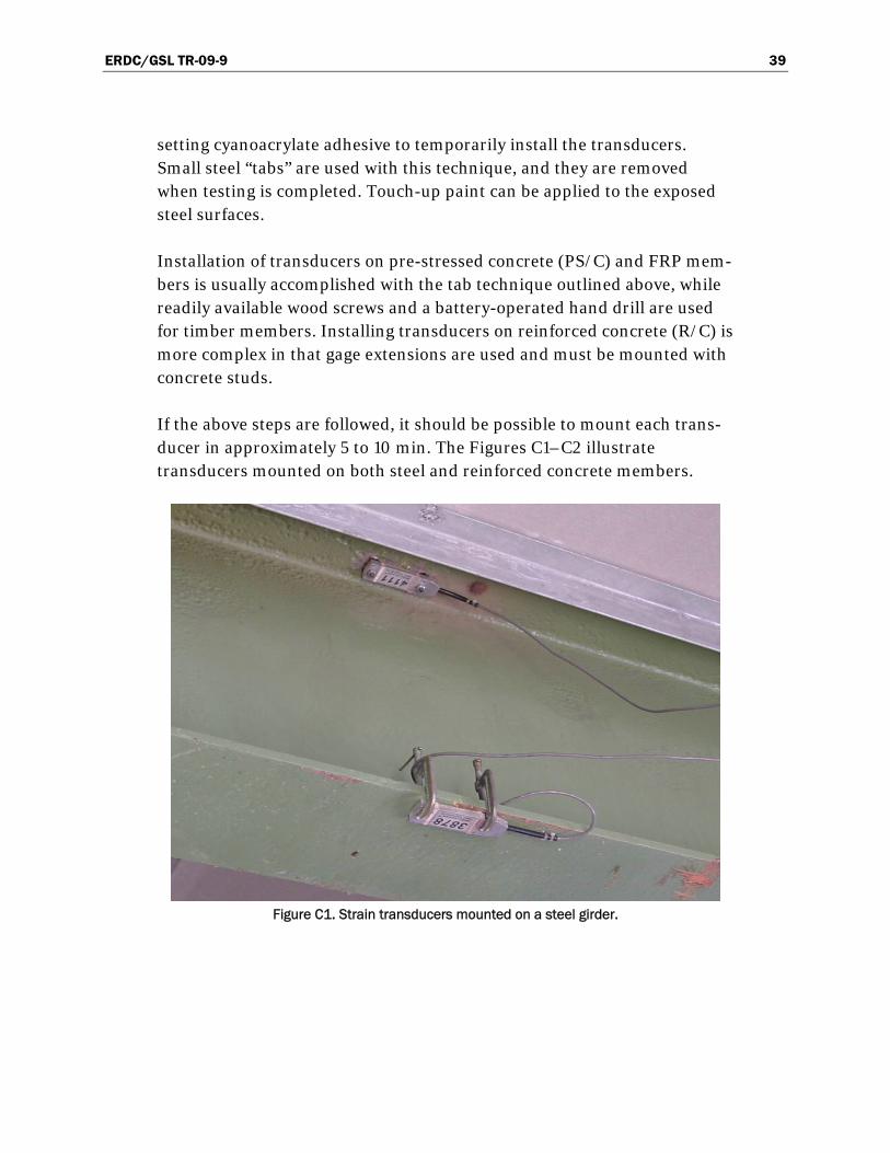
Installation of transducers on pre-stressed concrete (PS/C) and FRP mem-bers is usually accomplished with the tab technique outlined above, while readily available wood screws and a battery-operated hand drill are used for timber members. Installing transducers on reinforced concrete (R/C) is more complex in that gage extensions are used and must be mounted with concrete studs.

If the above steps are followed, it should be possible to mount each trans-ducer in approximately 5 to 10 min. The Figures C1–C2 illustrate transducers mounted on both steel and reinforced concrete members.

Figure C1. Strain transducers mounted on a steel girder.

ERDC/GSL TR-09-9 40

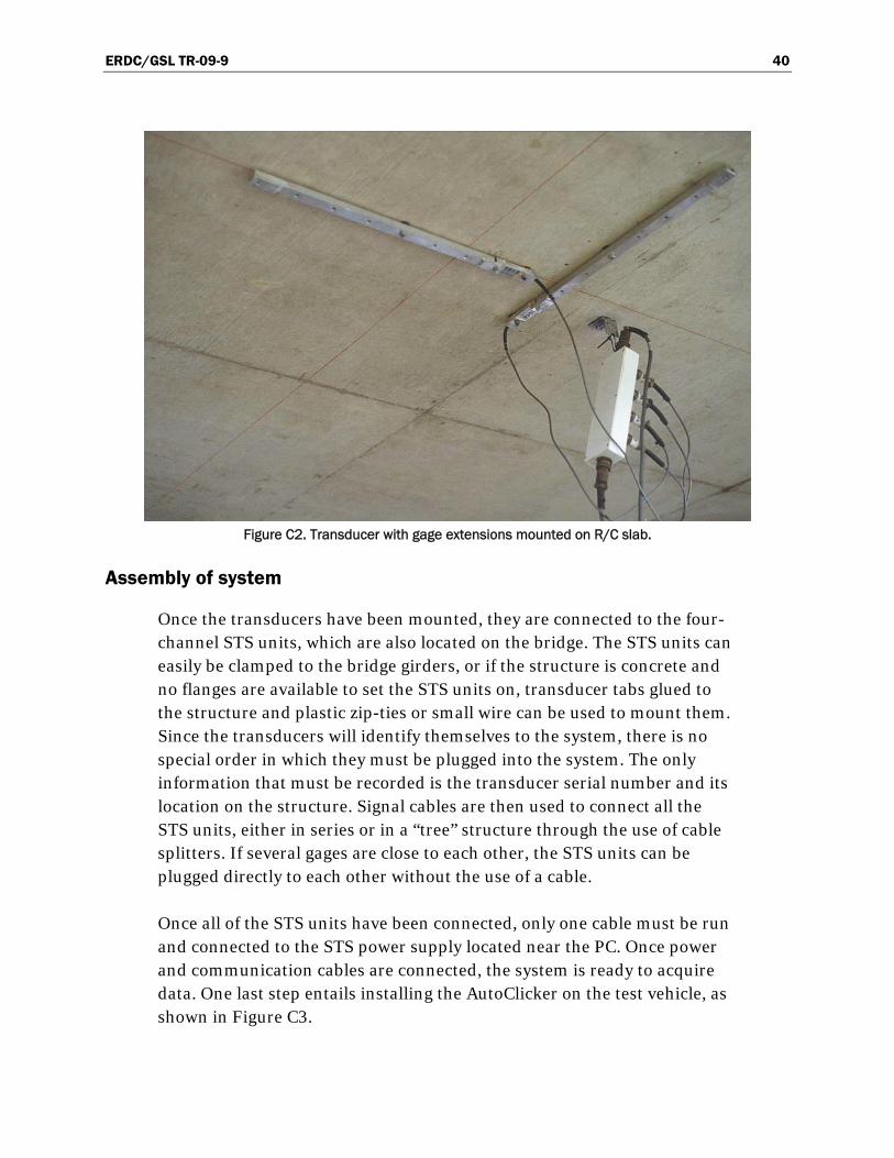
Figure C2. Transducer with gage extensions mounted on R/C slab.

Assembly of system

Once the transducers have been mounted, they are connected to the four-channel STS units, which are also located on the bridge. The STS units can easily be clamped to the bridge girders, or if the structure is concrete and no flanges are available to set the STS units on, transducer tabs glued to the structure and plastic zip-ties or small wire can be used to mount them. Since the transducers will identify themselves to the system, there is no special order in which they must be plugged into the system. The only information that must be recorded is the transducer serial number and its location on the structure. Signal cables are then used to connect all the STS units, either in series or in a “tree” structure through the use of cable splitters. If several gages are close to each other, the STS units can be plugged directly to each other without the use of a cable.

Once all of the STS units have been connected, only one cable must be run and connected to the STS power supply located near the PC. Once power and communication cables are connected, the system is ready to acquire data. One last step entails installing the AutoClicker on the test vehicle, as shown in Figure C3.

ERDC/GSL TR-09-9 41

Figure C3. AutoClicker mounted on test vehicle.

Establishing load vehicle positions

Once the structure is instrumented and the loading vehicle prepared, some reference points must be established on the deck in order to determine where the vehicle will cross. This process is important so that future analy-sis comparisons can be made with the loading vehicle in the same loca-tions as it was in the field. Therefore, a “zero” or initial reference point is selected and usually corresponds to the point on the deck directly above the abutment bearing and the centerline of one of the fascia beams. All other measurements on the deck will then be related to this zero reference point. For concrete T-beams, box beams, and slabs, this can correspond to where the edge of the slab or the beam web meets the face of the abut-ment. If the bridge is skewed, the first point encountered from the direc-tion of travel is used. In any case, it should be a point that is easily located on the drawings of the structure.

ERDC/GSL TR-09-9 42

Once the zero reference location is known, the lateral load paths for the vehicle are determined. Often, the painted roadway lines are used for the driver to follow if they are in convenient locations. For example, for a two-lane bridge, a northbound shoulder line will correspond to Y1 (passenger-side wheel), the center dashed line to Y2 (center of truck), and the southbound shoulder line to Y3 (driver’s side wheel). Often, the structure will be symmetrical with respect to its longitudinal centerline. If so, it is good practice is to take advantage of this symmetry by selecting three “Y” locations that are also symmetric. This will allow for a data quality check since the response should be very similar, say, on the middle beam if the truck is on the left side of the bridge or the right side of the bridge. In general, it is best to have the truck travel in each lane (at least on the lane line) and also as close to each shoulder or sidewalk as possible. When the deck layout is completed, the loading vehicle’s axle weights and dimen-sions are recorded.

Running the load tests

After the structure has been instrumented and the reference system laid out on the bridge deck, the actual testing procedures are completed. The WinSTS software is initialized and configured. When all personnel are ready to commence the test, traffic control is initiated and the Run Test option is selected, which places the system in an activated state. When the truck passes over the first deck mark, the AutoClicker is tripped and data are being collected at the specified sample rate. An effort is made to get the truck across with no other traffic on the bridge. When the rear axle of the vehicle completely crosses over the structure, the data collection is stopped and several strain histories evaluated for data quality. Usually, at least two passes are made at each Y position to ensure data reproducibility, and then if conditions permit, high-speed or dynamic tests are completed.

The use of a moving load as opposed to placing the truck at discrete locations has two major benefits. First, the testing can be completed much quicker, meaning there is less impact on traffic. Second, and more importantly, much more information can be obtained (both quantitative and qualitative). Discontinuities or unusual responses in the strain histories, which are often signs of distress, can be easily detected. Since the load position is monitored as well, it is easy to determine what loading conditions cause the observed effects. If readings are recorded only at discrete truck locations, the risk of losing information between the points

ERDC/GSL TR-09-9 43

is great. The advantages of continuous readings have been proven over and over again.

When the testing procedures are complete, the instrumentation is removed and any touch-up work completed.

ERDC/GSL TR-09-9 44

Appendix D: Specifications – BDI Strain Transducers

Figure D1. BDI strain transducer.

Table D1. Strain transducer specifications.

Effective gage length: 3.0 in (76.2 mm). Extensions available for use on R/C structures. Overall Size: 4.4 in x 1.2 in x 0.5 in (110 mm x 33 mm x 12 mm).Cable Length: 10 ft (3 m) standard, any length available.Material: Aluminum Circuit: Full wheatstone bridge with four active 350Ω foil gages, 4-wire hookup.Accuracy: ± 2%, individually calibrated to NIST standards.Strain Range: Approximately ±4000 με.Force req’d for 1000 με: Approximately 9 lbs. (40 N).Sensitivity: Approximately 500 με/mV/V,Weight: Approximately 3 oz. (88 g),Environmental: Built-in protective cover, also water resistant.Temperature Range: -60°F to 250°F (-50°C to 120°C ) operation range.Cable: BDI RC-187: 22 gage, two individually shielded pairs w/drain. Options: Fully waterproofed, Heavy-duty cable, Special quick-lock connector. Attachment Methods: C-clamps or threaded mounting tabs & quick-setting adhesive.

ERDC/GSL TR-09-9 45

Appendix E: Specifications – BDI Structural Testing System

Figure E1. BDI structural testing system.

Table E1. Structural testing system specifications.

Channels 4 to 128, expandable in multiples of four

Hardware Accuracy

± 0.2% (2% for strain transducers)

Sample Rates 0.01 to 1,000 Hz sample rate. Internal over-sampling rate is 15 KHz.

Max Test Lengths

20 minutes at 100 Hz. 128K samples per channel maximum test length.

Gain Levels 1, 250, 500, 1000

Digital Filter Fixed by selected sample rate

Analog Filter 200 Hz, -3db, 3rd order Bessel

Max. Input Voltage

±10V

Power 85 - 264 VAC, 47-440 Hz -25 to 55 °C

12VDC Power External inverter included

Excitation Voltages: Standard: LVDT:

5VDC @ 200mA ±15VDC @ 200mA

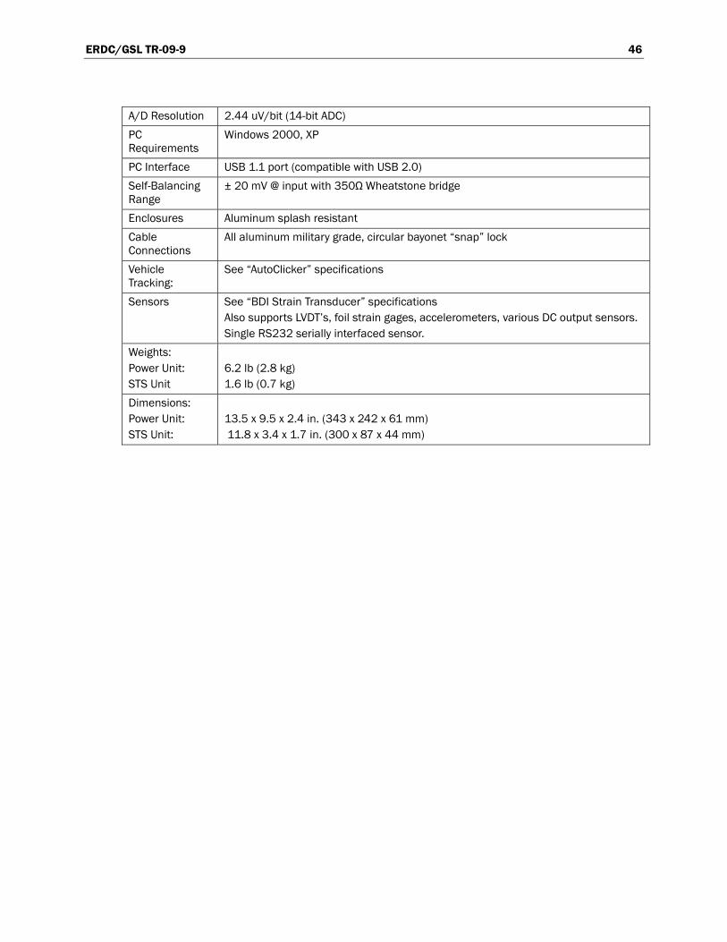
ERDC/GSL TR-09-9 46

A/D Resolution 2.44 uV/bit (14-bit ADC)

PC Requirements

Windows 2000, XP

PC Interface USB 1.1 port (compatible with USB 2.0)

Self-Balancing Range

± 20 mV @ input with 350Ω Wheatstone bridge

Enclosures Aluminum splash resistant

Cable Connections

All aluminum military grade, circular bayonet “snap” lock

Vehicle Tracking:

See “AutoClicker” specifications

Sensors See “BDI Strain Transducer” specifications Also supports LVDT’s, foil strain gages, accelerometers, various DC output sensors. Single RS232 serially interfaced sensor.

Weights: Power Unit: STS Unit

6.2 lb (2.8 kg) 1.6 lb (0.7 kg)

Dimensions: Power Unit: STS Unit:

13.5 x 9.5 x 2.4 in. (343 x 242 x 61 mm) 11.8 x 3.4 x 1.7 in. (300 x 87 x 44 mm)

ERDC/GSL TR-09-9 47

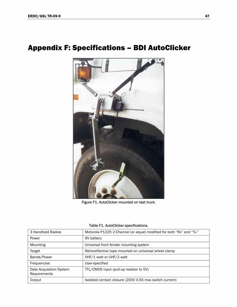
Appendix F: Specifications – BDI AutoClicker

Figure F1. AutoClicker mounted on test truck.

Table F1. AutoClicker specifications.

3 Handheld Radios Motorola P1225 2-Channel (or equal) modified for both “Rx” and “Tx.”

Power 9V battery

Mounting Universal front fender mounting system

Target Retroreflective tape mounted on universal wheel clamp

Bands/Power VHF/1 watt or UHF/2 watt

Frequencies User-specified

Data Acquisition System Requirements

TTL/CMOS input (pull-up resistor to 5V)

Output Isolated contact closure (200V 0.5A max switch current)

ERDC/GSL TR-09-9 48

Appendix G: Modeling and Analysis—The Integrated Approach

Introduction

In order for load testing to be a practical means of evaluating short- to medium-span bridges, it is apparent that testing procedures must be eco-nomic to implement in the field and the test results translatable into a load rating. A well-defined set of procedures must exist for the field applica-tions as well as for the interpretation of results. An evaluation approach based on these requirements was first developed at the University of Colo-rado during a research project sponsored by the Pennsylvania Department of Transportation (PennDOT). Over several years, the techniques originat-ing from this project have been refined and expanded into a complete bridge rating system.

The ultimate goal of the Integrated Approach is to obtain realistic rating values for highway bridges in a cost-effective manner. This is accom-plished by measuring the response behavior of the bridge due to a known load and determining the structural parameters that produce the meas-ured responses. With the availability of field measurements, many struc-tural parameters in the analytical model can be evaluated that are otherwise conservatively estimated or ignored entirely. Items that can be quantified through this procedure include the effects of structural geome-try, effective beam stiffness, realistic support conditions, effects of para-pets and other non-structural components, lateral load transfer capabilities of the deck and transverse members, and the effects of damage or deterioration. Often, bridges are rated poorly because of inaccurate representations of the structural geometry or because the material and/or cross-sectional properties of main structural elements are not well defined. A realistic rating can be obtained, however, when all of the relevant struc-tural parameters are defined and implemented in the analysis process.

One of the most important phases of this approach is a qualitative evalua-tion of the raw field data. Much is learned during this step to aid in the rapid development of a representative model.

ERDC/GSL TR-09-9 49

Initial data evaluation

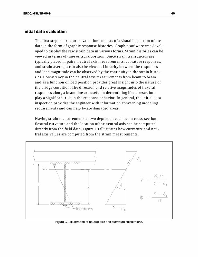
The first step in structural evaluation consists of a visual inspection of the data in the form of graphic response histories. Graphic software was devel-oped to display the raw strain data in various forms. Strain histories can be viewed in terms of time or truck position. Since strain transducers are typically placed in pairs, neutral axis measurements, curvature responses, and strain averages can also be viewed. Linearity between the responses and load magnitude can be observed by the continuity in the strain histo-ries. Consistency in the neutral axis measurements from beam to beam and as a function of load position provides great insight into the nature of the bridge condition. The direction and relative magnitudes of flexural responses along a beam line are useful in determining if end restraints play a significant role in the response behavior. In general, the initial data inspection provides the engineer with information concerning modeling requirements and can help locate damaged areas.

Having strain measurements at two depths on each beam cross-section, flexural curvature and the location of the neutral axis can be computed directly from the field data. Figure G1 illustrates how curvature and neu-tral axis values are computed from the strain measurements.

Figure G1. Illustration of neutral axis and curvature calculations.

ERDC/GSL TR-09-9 50

The consistency in the N.A. values between beams indicates the degree of consistency in beam stiffness. Also, the consistency of the N.A. measure-ment on a single beam as a function of truck position provides a good quality check for that beam. If for some reason a beam’s stiffness changes with respect to the applied moment (i.e. loss of composite action or loss of effective flange width due to a deteriorated deck), it will be observed by a shift in the N.A. history.

Since strain values are translated from a function of time into a function of vehicle position on the structure and the data acquisition channel and the truck position tracked, a considerable amount of book keeping is required to perform the strain comparisons. In the past, this required manipulation of result files and spreadsheets which was tedious and a major source of error. This process in now performed automatically by the software and all of the information can be verified visually.

Finite element modeling and analysis

The primary function of the load test data is to aid in the development of an accurate finite element model of the bridge. Finite element analysis is used because it provides the most general tool for evaluating various types of structures. Since a comparison of measured and computed responses is performed, it is necessary that the analysis be able to represent the actual response behavior. This requires that actual geometry and boundary conditions be realistically represented. In maintaining reasonable model-ing efforts and computer run times, a certain amount of simplicity is also required, so a planar grid model is generated for most structures and lin-ear-elastic responses are assumed. A grid of frame elements is assembled in the same geometry as the actual structure. Frame elements represent the longitudinal and transverse members of the bridge. The load transfer characteristics of the deck are provided by attaching plate elements to the grid. When end restraints are determined to be present, elastic spring ele-ments having both translational and rotational stiffness terms are inserted at the support locations.

Loads are applied in a manner similar to the actual load test. A model of the test truck, defined by a two-dimensional group of point loads, is placed on the structure model at discrete locations along the same path that the test truck followed during the load test. Gage locations identical to those in the field are also defined on the structure model so that strains can be computed at the same locations under the same loading conditions.

ERDC/GSL TR-09-9 51

Evaluation of rotational end restraint

A common requirement in structural identification is the need to deter-mine effective spring stiffnesses that best represent in-situ support condi-tions. Where as it is generally simple to evaluate a spring constant in terms of moment per rotation, the value generally has little meaning to the engi-neer. A more conceptual approach is to evaluate the spring stiffness as a percentage of a fully restrained condition. For example: 0% being a pinned condition and 100% being fixed. This is best accomplished by examining the ratio of the beam or slab stiffness to the rotational stiffness of the sup-port.

As an illustration, a point load is applied to a simple beam with elastic sup-ports, see Figure G2. By examining the moment diagram, it is apparent that the ratio of the end moment to the midspan moment (Me/Mm) equals 0.0 if the rotational stiffness (Kr) of the springs is equal to 0.0. Conversely, if the value of Kr is set to infinity (rigid) the moment ratio will equal 1.0. If a fixity term is defined as the ratio (Me/Mm), which ranges from 0 to 100 percent, a more conceptual measure of end restraint can be obtained.

The next step is to relate the fixity term to the actual spring stiffness (Kr). The degree to which the Kr effects the fixity term depends on the beam or slab stiffness to which the spring is attached. Therefore the fixity term must be related to the ratio of the beam/spring stiffness. Figure G3 con-tains a graphical representation of the end restraint effect on a simple beam. Using the graph, a conceptual measure of end-restraint can be defined after the beam and spring constants are evaluated through struc-tural identification techniques.

ERDC/GSL TR-09-9 52

P

L/2 L/2

M e

Mm

K r EI

Figure G2. Moment diagram of beam with rotational end restraint.

End Restraint Fixity Terms

0

0.1

0.2

0.3

0.4

0.5

0.6

0.7

0.8

0.9

1

0 1 2 3 4 5 6 7 8 9 10

(EI)/(KL) - Radians

En

d -

Mid

span

Mo

men

t R

atio

(M

end

/ M

mid

)

Figure G3. Relationship between spring stiffness and fixity ratio.

ERDC/GSL TR-09-9 53

Model correlation and parameter modification

The accuracy of the model is determined numerically by the analysis using several statistical relationships and through visual comparison of the strain histories. The numeric accuracy values are useful in evaluating the effect of any changes to the model, where as the graphical representations provide the engineer with the best perception for why the model is responding differently than the measurements indicate. Member proper-ties that cannot be accurately defined by conventional methods or directly from the field data are evaluated by comparing the computed strains with the measured strains. These properties are defined as variable and are evaluated such that the best correlation between the two sets of data is obtained. It is the engineer’s responsibility to determine which parameters need to be refined and to assign realistic upper and lower limits to each parameter. The evaluation of the member property is accomplished with the aid of a parameter identification process (optimizer) built into the analysis. In short, the process consists of an iterative procedure of analy-sis, data comparison, and parameter modification. It is important to note that the optimization process is merely a tool to help evaluate various modeling parameters. The process works best when the number of parameters is minimized and reasonable initial values are used.

During the optimization process, various error values are computed by the analysis program that provides a quantitative measure of the model accu-racy and improvement. The error is quantified in four different ways, each providing a different perspective of the model’s ability to represent the actual structure; an absolute error, a percent error, a scale error and a correlation coefficient.

The absolute error is computed from the absolute sum of the strain differences. Algebraic differences between the measured and theoretical strains are computed at each gage location for each truck position used in the analysis; therefore, several hundred strain comparisons are generally used in this calculation. This quantity is typically used to determine the relative accuracy from one model to the next and to evaluate the effect of various structural parameters. It is used by the optimization algorithm as the objective function to minimize. Because the absolute error is in terms of micro-strain (mε) the value can vary significantly depending on the magnitude of the strains, the number of gages and number of different loading scenarios. For this reason, it has little conceptual value except for determining the relative improvement of a particular model.

ERDC/GSL TR-09-9 54

A percent error is calculated to provide a better qualitative measure of accuracy. It is computed as the sum of the strain differences squared divided by the sum of the measured strains squared. The terms are squared so that error values of different sign will not cancel each other out, and to put more emphasis on the areas with higher strain magnitudes. A model with acceptable accuracy will usually have a percent error of less than 10%.

The scale error is similar to the percent error except that it is based on the maximum error from each gage divided by the maximum strain value from each gage. This number is useful because it is based only on strain measurements recorded when the loading vehicle is in the vicinity of each gage. Depending on the geometry of the structure, the number of truck positions, and various other factors, many of the strain readings are essen-tially negligible. This error function uses only the most relevant measurement from each gage.

Another useful quantity is the correlation coefficient, which is a meas-ure of the linearity between the measured and computed data. This value determines how well the shapes of the computed response histories match the measured responses. The correlation coefficient can have a value between 1.0 (indicating a perfect linear relationship) and -1.0 (exact oppo-site linear relationship). A good model will generally have a correlation coefficient greater than 0.90. A poor correlation coefficient is usually an indication that a major error in the modeling process has occurred. This is generally caused by poor representations of the boundary conditions or the loads were applied incorrectly (i.e. truck traveling in wrong direction).

The following table contains the equations used to compute each of the statistical error values:

ERDC/GSL TR-09-9 55

Table G1. Error functions.

Error Function Equation

Absolute error |c - m| εε

Percent error ( ) )2m( / c - m2 εεε

Scale error

|gagem|

|gagec - m|

ε

εεmax

max

Correlation coefficient

)2c - c()2m - m(

)c - c)(m - m(

εεεε

εεεε

In addition to the numerical comparisons made by the program, periodic visual comparisons of the response histories are made to obtain a concep-tual measure of accuracy. Again, engineering judgment is essential in determining which parameters should be adjusted so as to obtain the most accurate model. The selection of adjustable parameters is performed by determining what properties have a significant effect on the strain comparison and determining which values cannot be accurately estimated through conventional engineering procedures. Experience in examining the data comparisons is helpful; however, two general rules apply concern-ing model refinement. When the shapes of the computed response histo-ries are similar to the measured strain records but the magnitudes are incorrect this implies that member stiffness must be adjusted. When the shapes of the computed and measured response histories are not very similar then the boundary conditions or the structural geometry are not well represented and must be refined.

In some cases, an accurate model cannot be obtained, particularly when the responses are observed to be non-linear with load position. Even then, a great deal can be learned about the structure and intelligent evaluation decisions can be made.

ERDC/GSL TR-09-9 56

Appendix H: Load Rating Procedures

A load-rating factor is a numeric value indicating a structure’s ability to carry a specific load. Load rating factors were computed by applying stan-dard design loads along with the structure’s self-weight and asphalt over-lay. Rating factors are computed for various structural components and are equal to the ratio of the component’s live load capacity and the live load applied to that component; including all appropriate load factors. A load-rating factor greater than 1.0 indicates a member’s capacity exceeds the applied loads with the desired factors of safety. A rating factor less than 1.0 indicates a member is deficient such that a specific vehicle cannot cross the bridge with the desired factor of safety. A number near 0.0 indi-cates the structure cannot carry its own dead weight and maintain the desired safety factor. The lowest component rating-factor generally controls the load rating of the entire structure. Additional factors are applied to account for variability in material, load application, and dynamic effects. Two levels of load rating are performed for the bridge. An Inventory Level rating corresponds to the design stress levels and/or fac-tors of safety and represents the loads that can be applied on a daily basis. The Operating Rating levels correspond to the maximum load limits above which the structure may experience damage or failure.

For borderline bridges (those that calculations indicate a posting is required), the primary drawback to conventional bridge rating is an over-simplified procedure for estimating the load applied to a given beam (i.e. wheel load distribution factors) and a poor representation of the beam itself. Due to lack of information and the need for conservatism, material and cross-section properties are generally over-estimated and beam end supports are assumed to be simple when in fact even relatively simple beam bearings have a substantial effect on the midspan moments. Inaccuracies associated with conservative assumptions are compounded with complex framing geometries. From an analysis standpoint, the goal here is to generate a model of the structure that is capable of reproducing the measured strains. Decisions concerning load rating are then based on the performance of the model once it is proven to be accurate.

The main purpose for obtaining an accurate model is to evaluate how the bridge will respond when standard design loads, rating vehicles or permit

ERDC/GSL TR-09-9 57

loads are applied to the structure. Since load testing is generally not per-formed with all of the vehicles of interest, an analysis must be performed to determine load-rating factors for each truck type. Load rating is accom-plished by applying the desired rating loads to the model and computing the stresses on the primary members. Rating factors are computed using the equation specified in the AASHTO Manual for Condition Evaluation of Bridges - see Equation (H1).

It is important to understand that diagnostic load testing and the inte-grated approach are most applicable to obtaining Inventory (service load) rating values. This is because it is assumed that all of the measured and computed responses are linear with respect to load. The integrated approach is an excellent method for estimating service load stress values but it generally provides little additional information regarding the ulti-mate strength of particular structural members. Therefore, operating rat-ing values must be computed using conventional assumptions regarding member capacity. This limitation of the integrated approach is not viewed as a serious concern, however, because load responses should never be permitted to reach the inelastic range.

Operating and/or Load Factor rating values must also be computed to ensure a factor of safety between the ultimate strength and the maximum allowed service loads. The safety to the public is of vital importance but as long as load limits are imposed such that the structure is not damaged then safety is no longer an issue.

Following is an outline describing how field data is used to help in developing a load rating for the superstructure. These procedures will only complement the rating process, and must be used with due consideration to the substructure and inspection reports.

Preliminary investigation: Verification of linear and elastic behavior through continuity of strain histories, locate neutral axis of flexural mem-bers, detect moment resistance at beam supports, and qualitatively evalu-ate behavior.

Develop representative model: Use graphic pre-processors to repre-sent the actual geometry of the structure, including span lengths, girder spacing, skew, transverse members, and deck. Identify gage locations on model identical to those applied in the field.

ERDC/GSL TR-09-9 58

Simulate load test on computer model: Generate 2-dimensional model of test vehicle and apply to structure model at discrete positions along same paths defined during field tests. Perform analysis and compute strains at gage location for each truck position.

Compare measured and initial computed strain values: Various global and local error values at each gage location are computed and visual comparisons made with post-processor.

Evaluate modeling parameters: Improve model based on data comparisons. Engineering judgment and experience is required to deter-mine which variables are to be modified. A combination of direct evaluation techniques and parameter optimization are used to obtain a realistic model. General rules have been defined to simplify this operation.

Model evaluation: In some cases it is not desirable to rely on secondary stiffening effects if it is likely they will not be effective at higher load levels. It is beneficial, though, to quantify their effects on the structural response so that a representative computer model can be obtained. The stiffening effects that are deemed unreliable can be eliminated from the model prior to the computation of rating factors. For instance, if a non-composite bridge is exhibiting composite behavior, then it can conservatively be ignored for rating purposes. However, if it has been in service for 50 years and it is still behaving compositely, chances are that very heavy loads have crossed over it and any bond-breaking would have already occurred. Therefore, probably some level of composite behavior can be relied upon. When unintended composite action is allowed in the rating, additional load limits should be computed based on an allowable shear stress between the steel and concrete and an ultimate load of the non-composite structure.

Perform load rating: Apply HS-20 and/or other standard design, rating and permit loads to the calibrated model. Rating and posting load configuration recommended by AASHTO are shown in Figure H1.

The same rating equation specified by the AASHTO - Manual for the Condition Evaluation of Bridges is applied:

ERDC/GSL TR-09-9 59

)( ) ( ) (( )IMLL

PDW DC- C = RF

L

PDWDC

+±−

γγγγ

(H1)

where:

RF = rating factor for individual member C = member capacity γDC = LRFD load factor for structural components and

attachments D = dead-load effect due to structural components γDW = LRFD load factor for wearing surfaces and utilities DW = dead-load effect due to wearing surface and utilities γP = LRFD load factor for permanent loads other than

dead loads = 1.0 P = permanent loads other than dead loads LL = live-load effect IM = impact effect, either AASHTO or measured.

The only difference between this rating technique and standard beam rating programs is that a more realistic model is used to determine the dead-load and live-load effects. Two-dimensional loading techniques are applied because wheel load distribution factors are not applicable to a planar model. Stress envelopes are generated for several truck paths, envelopes for paths separated by normal lane widths are combined to determine multiple lane loading effects.

Consider other factors: Other factors such as the condition of the deck and/or substructure, traffic volume, and other information in the inspec-tion report should be taken into consideration and the rating factors adjusted accordingly.

ERDC/GSL TR-09-9 60

Figure H1. AASHTO rating and posting load configurations.

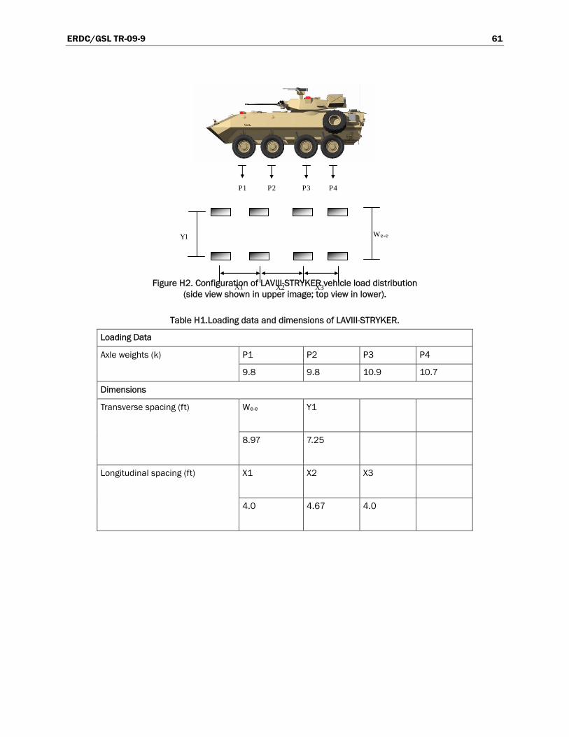
ERDC/GSL TR-09-9 61

P1 P2 P3 P4

Figure H2. Configuration of LAVIII-STRYKER vehicle load distribution (side view shown in upper image; top view in lower).

X1 X2 X3

We-eY1

Table H1.Loading data and dimensions of LAVIII-STRYKER.

Loading Data

P1 P2 P3 P4 Axle weights (k)

9.8 9.8 10.9 10.7

Dimensions

We-e Y1 Transverse spacing (ft)

8.97 7.25

X1 X2 X3 Longitudinal spacing (ft)

4.0 4.67 4.0

ERDC/GSL TR-09-9 62

Figure H3. Configuration of HETS vehicle load distribution (side view shown in upper image; top view in lower).

Table H2. Loading data and dimensions of HETS.

Loading Data

P1 P2 P3 P4 P5 P6 P7 P8 P9 Axle loads (k)

21.7 22.3 21.7 19.9 27.0 29.7 28.0 28.0 31.4

Dimensions

We-e Y1 Y2 Y3 Y4 Y5 Transverse spacing (ft)

12.0 1.67 1.12 4.85 1.12 1.67

X1 X2 X3 X4 X5 X6 X7 X8 Longitudinal spacing (ft)

12.92 5.0 5.0 15.94 5.94 5.94 5.94 5.94

X1 X2 X3 X4 X5 X6 X7 X8

Y1 Y2

Y3

Y4 Y5

We-e

P1 P2 P3 P4 P5 P6 P7 P8 P9

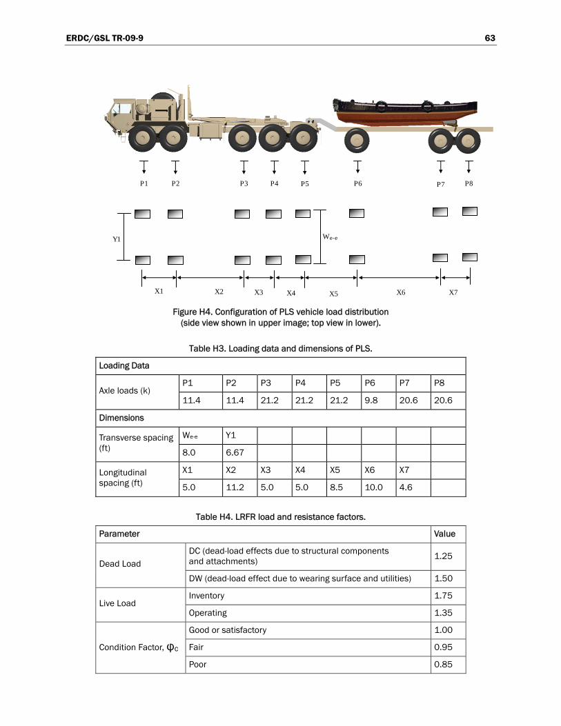
ERDC/GSL TR-09-9 63

Figure H4. Configuration of PLS vehicle load distribution (side view shown in upper image; top view in lower).

Table H3. Loading data and dimensions of PLS.

Loading Data

P1 P2 P3 P4 P5 P6 P7 P8 Axle loads (k)

11.4 11.4 21.2 21.2 21.2 9.8 20.6 20.6

Dimensions

We-e Y1 Transverse spacing (ft) 8.0 6.67

X1 X2 X3 X4 X5 X6 X7 Longitudinal spacing (ft) 5.0 11.2 5.0 5.0 8.5 10.0 4.6

Table H4. LRFR load and resistance factors.

Parameter Value

DC (dead-load effects due to structural components and attachments)

1.25 Dead Load

DW (dead-load effect due to wearing surface and utilities) 1.50

Inventory 1.75 Live Load

Operating 1.35

Good or satisfactory 1.00

Fair 0.95 Condition Factor, φc

Poor 0.85

X1 X2

Y1 We-e

X3 X4 X6 X7 X5

P1 P2 P3 P4 P6 P8 P5 P7

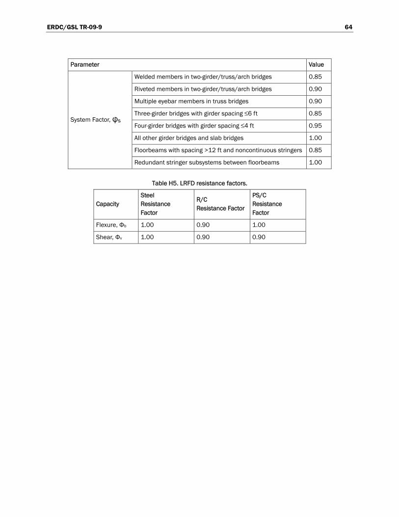
ERDC/GSL TR-09-9 64

Parameter Value

Welded members in two-girder/truss/arch bridges 0.85

Riveted members in two-girder/truss/arch bridges 0.90

Multiple eyebar members in truss bridges 0.90

Three-girder bridges with girder spacing ≤6 ft 0.85

Four-girder bridges with girder spacing ≤4 ft 0.95

All other girder bridges and slab bridges 1.00

Floorbeams with spacing >12 ft and noncontinuous stringers 0.85

System Factor, φs

Redundant stringer subsystems between floorbeams 1.00

Table H5. LRFD resistance factors.

Capacity Steel Resistance Factor

R/C Resistance Factor

PS/C Resistance Factor

Flexure, Φb 1.00 0.90 1.00

Shear, Φv 1.00 0.90 0.90

REPORT DOCUMENTATION PAGE Form Approved

OMB No. 0704-0188 Public reporting burden for this collection of information is estimated to average 1 hour per response, including the time for reviewing instructions, searching existing data sources, gathering and maintaining the data needed, and completing and reviewing this collection of information. Send comments regarding this burden estimate or any other aspect of this collection of information, including suggestions for reducing this burden to Department of Defense, Washington Headquarters Services, Directorate for Information Operations and Reports (0704-0188), 1215 Jefferson Davis Highway, Suite 1204, Arlington, VA 22202-4302. Respondents should be aware that notwithstanding any other provision of law, no person shall be subject to any penalty for failing to comply with a collection of information if it does not display a currently valid OMB control number. PLEASE DO NOT RETURN YOUR FORM TO THE ABOVE ADDRESS.

1. REPORT DATE (DD-MM-YYYY) May 2009

2. REPORT TYPE Final report

3. DATES COVERED (From – To)

5a. CONTRACT NUMBER

5b. GRANT NUMBER

4. TITLE AND SUBTITLE

Field Testing and Load Rating Report, Bridge FSBR-514, Fort Shafter, Hawaii

5c. PROGRAM ELEMENT NUMBER

5d. PROJECT NUMBER

5e. TASK NUMBER

6. AUTHOR(S)

Brett Commander, Wilmel Varela-Ortiz, Terry R. Stanton, and Henry Diaz-Alvarez

5f. WORK UNIT NUMBER

7. PERFORMING ORGANIZATION NAME(S) AND ADDRESS(ES) Bridge Diagnostics, Inc. 1965 57th Court North, Suite 106 Boulder, CO 80301-2826;

8. PERFORMING ORGANIZATION REPORT NUMBER

U.S. Army Engineer Research and Development Center Geotechnical and Structures Laboratory 3909 Halls Ferry Road, Vicksburg, MS 39180-6199

ERDC/GSL TR-09-9

9. SPONSORING / MONITORING AGENCY NAME(S) AND ADDRESS(ES) 10. SPONSOR/MONITOR’S ACRONYM(S)

11. SPONSOR/MONITOR’S REPORT NUMBER(S)

Headquarters, Installation Management Command (IMCOM) Arlington, VA 22202

12. DISTRIBUTION / AVAILABILITY STATEMENT Approved for public release; distribution is unlimited.

13. SUPPLEMENTARY NOTES

14. ABSTRACT

Bridge Diagnostics, Inc., was contracted by the U.S. Army Corps of Engineers to perform live-load testing and load rating on Bridge FSBR-514 on Walker Road over Kahauiki Stream, Fort Shafter, Hawaii, in conjunction with three other structures—Bridge FSBR-201, FSBR-1608, and ERBR-9. A primary goal of the live-load testing was to determine the relative effects of different military load configurations. A second goal was to use the measured load responses to verify and calibrate a finite element model of the structure.

The load test results indicated that the culvert was relatively stiff and did a good job of distributing load. Load ratings resulting from the field-verified model indicated that all examined load configurations could cross the bridge within inventory (design) limits.

Load ratings were computed in accordance the American Association of State Highway and Transportation Officials’ AASHTO LRFD bridge design specifications (2004) and Manual for the condition evaluation and load and resistance factor rating of highway bridges (2003).

15. SUBJECT TERMS Concrete box culvert Distribution factor

Finite element analyses Load rating

Load test Military vehicles

16. SECURITY CLASSIFICATION OF: 17. LIMITATION OF ABSTRACT

18. NUMBER OF PAGES

19a. NAME OF RESPONSIBLE PERSON

a. REPORT

UNCLASSIFIED

b. ABSTRACT

UNCLASSIFIED

c. THIS PAGE

UNCLASSIFIED 72 19b. TELEPHONE NUMBER (include area code)

Standard Form 298 (Re . 8-98) vPrescribed by ANSI Std. 239.18