Embed Size (px)
Citation preview
1
Draft Revision Date: 2/24/2016
Abstract— This report describes the use of a support vector
machines with a novel kernel, to determine the breathing rate and
inhalation duration of a fire fighter wearing a Self-Contained
Breathing Apparatus. With this information, an incident
commander can monitor the firemen in his command for
exhaustion and ensure timely rotation of personnel to ensure
overall fire fighter safety.
Index Terms - ???
I. INTRODUCTION
he Enhanced Situational Awareness in Firefighting
Emergencies project seeks to expand the knowledge
available about the incident in an integrated manner and make
this data available to firefighting incident commanders and
other firefighters working the incident.
A. Firefighting Data Collection Systems
The intention is to use the existing communication systems
with minimal changes to the certified and approved systems
currently in use. Currently, the primary tools available for
communication and data collection are analog or digital radios.
Ultrahigh frequency (UHF) radios are used in a network where
the radio frequency is the shared resource. The prevalence of
these systems is a reliance on low cost and low complexity that
guarantees the systems robustness and availability. Another
advantage is that firefighters can join or dropout as needed
resulting in a very flexible network that allows for a high degree
of autonomy for the individual firefighters. Thus any system
designed to operate in this environment must rely on local
processing of data related to each firefighter and communicate
only pertinent information without interfering with voice
communications.
The disadvantages to using a system like this are that the
voice communications reflect only what the firefighter wishes
to communicate about his perceptions of the situations he is in.
The data may be incomplete, since the firefighter’s focus is
localized to the immediate tasks at hand. Further, because of the
focus, he may forget information since it is not part of the
immediate task. Additionally, there is information being
recorded by the microphones that is normally suppressed to
make the communications clearer.
This paper presents the beginnings of the process of
extracting additional data using the radio microphones in
Eric. Hamke, Department of Electrical and Computer Engineering,
University of New Mexico, Albuquerque, NM 87110 USA (e-mail:
conjunction with a small signal processing unit. From the
additional audio data, it is the hope that we will be able to detect
background noises, related to explosions, various alarms that
the fireman wears to warn of situations such as carbon
monoxide and hydrogen cyanide released by burning plastics,
Self-Contained Breathing Apparatus’ low air alarm and the
firefighter stationary or inactive sensors intended to alert other
firefighters when a firefighter is injured or overcome.
In addition, we can also monitor the regulator sounds of the
Self-Contained Breathing Apparatus (SCBA) to detect the
starting and ending time of the inhalation events. These times
can then be processed to compute the breathing rate and
inhalation duration. Further processing could compute the
accumulated inhalation durations to estimate the amount of air
remaining in the fire fighter’s air tank. This information and the
breathing rate combined with other physiological data could be
relayed back to the incident commander at regular intervals
using burst communication and can be encoded into the voice
codex used by the radios.
B. Previous Works
Others have studied the process of monitoring breathing
sounds with the intent to identify them as noise that needs to be
eliminated from a recording or speech processing system. The
breath sound can be mistaken by speech processing systems as
a fricative sound and result in a false positive detection of
certain phonemes. Several medical applications have focused in
determining breathing rates of patients on respirators [16]. The
work using intrusive devices such as a respiratory inductive
plethysmography net. The data from the strain gauges is then
processed using an Artificial Neural Network. Another medical
study involved segmenting simulated breathing cycles. The
process proposed by Li et.al, [17] involves using a gradient to
determine the start of breathing cycles in a tidal breathing
pattern. The second stage of the process is to examine the time
between starting cycles and their duration. Since a breath is a
long duration compared to phonemes and can last for 1 second
or more.
Another area of research involves speech related
applications. The intention in these applications is to identify
breathing artifacts and remove them from the speech. The
primary features used are based on cepstral or meI frequency
cepstral coefficients (MFCC). Price et al. automatic breath
detection methods of speech signals were based on cepstral
coefficients and used Gaussian Mixture Model (GMM) as the
classifier, and achieved a detection rate of 93% [18], Wightman
and Ostendorf algorithm uses Bayesian classifier and achieved
Eric E. Hamke, Ramiro Jordan, Manel Ramon-Martinez
Breath Activity Detection Algorithm
T
2
Draft Revision Date: 2/24/2016
a detection rate of 91.3% [19]. Ruinskiy and Lavner applied
algorithm of automatic breath detection in speech and songs
based on MFCC parameters, short-time energy, ZCR (zero-
crossing rate), spectral slope, and duration [1], They introduced
also a method of edge detection, They achieved precision/recall
rate 97,6%/95.7%. Nakano et al. described detailed acoustic
analysis of breath sounds using MFCC parameters and Hidden
Markov Models [20]. The result was 97.5%/77.7% rates for
unaccompanied singing voice.
There are also many works performing breath detection as
one of many audio events in audio retrieval systems. Most of
them use MFCC or LPC (Linear Predictive Coding) parameters
[21]. In Classification the extracted feature vectors are assigned
to one of a set of classes. In MARSYAS, the Gaussian (MAP),
Gaussian Mixture Model (GMM) and K−NN families of
statistical Pattern Recognition classifiers are supported. Two
case studies of classification have been implemented and
evaluated in our system: a music/speech classifier and a genre
classifier. The music/speech classifier achieves a 90.1%
classification accuracy.
M. Igras, B. Ziolko [23]propose a method involving both
temporal and spectral features. The time domain analysis of the
extracted breaths determines the length and energy (normalized
in reference to the entire speech signal) is computed. These
features are combined with a discrete wavelet analysis. Finally
the wavelet features and the time features are classified using a
dynamic time warping algorithm, where the time-axis
fluctuation is approximately modeled with a nonlinear warping
function .Igra et. al., reported a 94.7% success at detecting
breaths with this approach.
S. Borys and M. Hasegawa-Johnson investigated several
techniques including Hidden Markov Models and Support
Vector Machines (SVM). They trained groups of SVM
classifiers that could detect different landmarks. The first group
of trained classifiers were designed to distinguish between
transitions for the features speech, sonorant, continuant and
syllabic. The second group of SVM classifiers was trained to
recognize positive and negative gradients where feature could
be speech, consonantal, sonorant, +consonantal/continuant. It is
not clear which types of kernels tey used. The kernels alluded
to include linear, radial basis function, polynomials and
sigmoid functions. Optimization for each different kernel
follows the same general procedure as the optimization for the
linear kernel. They concluded in their study that the SVMs they
developed had approximately 85% for Syllabic features and
97% for speech. The remaining features are in 95% for sonorant
and 90% for continuant.
The organization of the presentation starts by briefly
discussing the aspects of the SCBA for those who are not
familiar with the device. The next section is a survey of the two
methodologies reviewed, a pattern matching and the use of a
Linear Predictive Coefficients based filter. Additionally, the
third section will deal with the process of making the exemplars
used in the process. The feature extraction/enhancement
process is presented in the next section. In the detection section
we propose the use of machine learning (support vector
machines with a novel kernel). The final sections will deal with
the detection process.
II. ACOUSTIC PROPERTIES AND EFFECTS OF SELF-
CONTAINED BREATHING APPARATUS
The investigations focus on monitoring the breathing rate of
the firefighter using a Self-Contained Breathing Apparatus
(SCBA). The SCBA system is a pressure-demand air delivery
system. When a user inhales negative pressure within the mask
causes the regulator valve to open. Pressurized air enters the
mask producing a loud broadband hissing noise. The noise is
comparable in amplitude to the speech signal (fricative sound).
This signal is broadband and incoherent.
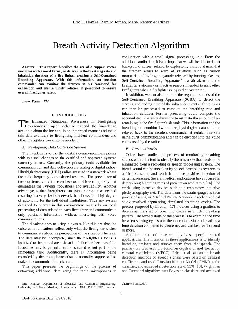
The mask (Fig. 1) is a rigid structure with a clear plastic face
plate and a flexible rubber seal that contacts the forehead
temples cheeks and chin of the wearer. The SCBA systemnoises
includes low air alarms and air regulator noises as well. [13]
Fig. 1. External and internal views of a commonly used SCBA mask showing
the voicemitter port. The breathing cycle is divided into four different phases:
[13]
III. THE METHODOLOGIES
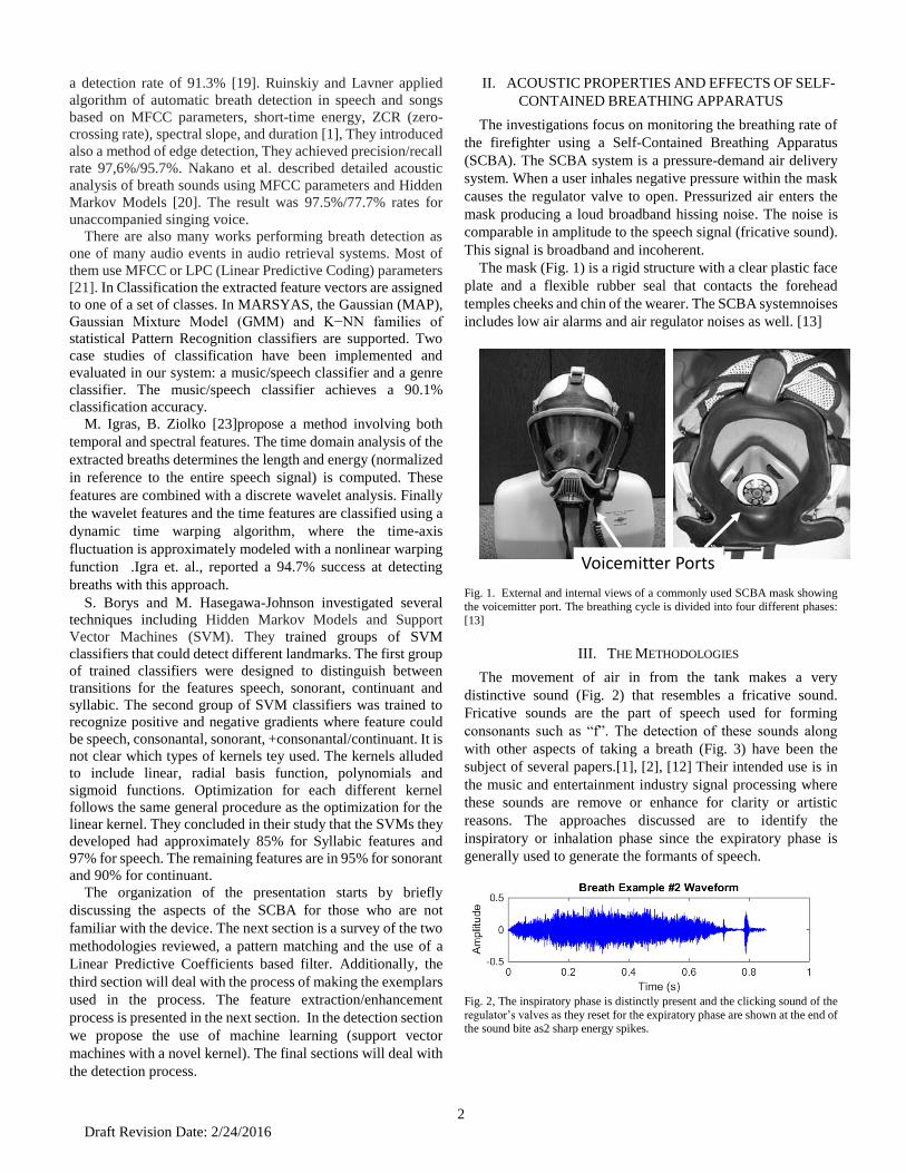
The movement of air in from the tank makes a very
distinctive sound (Fig. 2) that resembles a fricative sound.
Fricative sounds are the part of speech used for forming
consonants such as “f”. The detection of these sounds along
with other aspects of taking a breath (Fig. 3) have been the
subject of several papers.[1], [2], [12] Their intended use is in
the music and entertainment industry signal processing where
these sounds are remove or enhance for clarity or artistic
reasons. The approaches discussed are to identify the
inspiratory or inhalation phase since the expiratory phase is
generally used to generate the formants of speech.
Fig. 2, The inspiratory phase is distinctly present and the clicking sound of the
regulator’s valves as they reset for the expiratory phase are shown at the end of the sound bite as2 sharp energy spikes.
Voicemitter Ports
3
Draft Revision Date: 2/24/2016
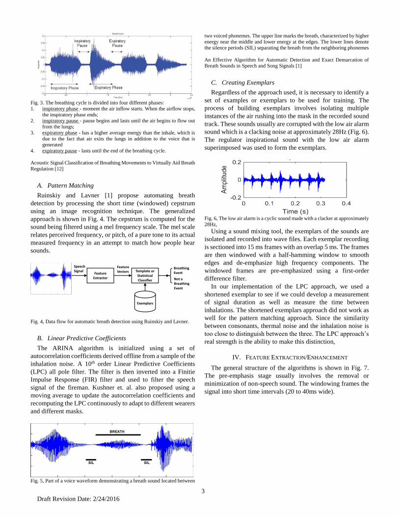
Fig. 3. The breathing cycle is divided into four different phases: 1. inspiratory phase - moment the air inflow starts. When the airflow stops,
the inspiratory phase ends;
2. inspiratory pause - pause begins and lasts until the air begins to flow out from the lungs;
3. expiratory phase - has a higher average energy than the inhale, which is
due to the fact that air exits the lungs in addition to the voice that is generated
4. expiratory pause - lasts until the end of the breathing cycle.
Acoustic Signal Classification of Breathing Movements to Virtually Aid Breath
Regulation [12]
A. Pattern Matching
Ruinskiy and Lavner [1] propose automating breath
detection by processing the short time (windowed) cepstrum
using an image recognition technique. The generalized
approach is shown in Fig. 4. The cepstrum is computed for the
sound being filtered using a mel frequency scale. The mel scale
relates perceived frequency, or pitch, of a pure tone to its actual
measured frequency in an attempt to match how people hear
sounds.
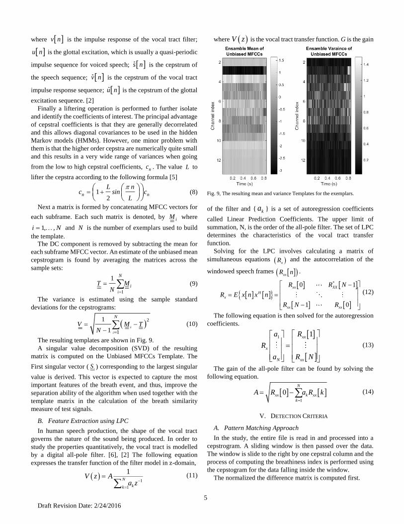
Fig. 4, Data flow for automatic breath detection using Ruinskiy and Lavner.
B. Linear Predictive Coefficients
The ARINA algorithm is initialized using a set of
autocorrelation coefficients derived offline from a sample of the
inhalation noise. A 10th order Linear Predictive Coefficients
(LPC) all pole filter. The filter is then inverted into a Finitie
Impulse Response (FIR) filter and used to filter the speech
signal of the fireman. Kushner et. al. also proposed using a
moving average to update the autocorrelation coefficients and
recomputing the LPC continuously to adapt to different wearers
and different masks.
Fig. 5, Part of a voice waveform demonstrating a breath sound located between
two voiced phonemes. The upper line marks the breath, characterized by higher
energy near the middle and lower energy at the edges. The lower lines denote the silence periods (SIL) separating the breath from the neighboring phonemes
An Effective Algorithm for Automatic Detection and Exact Demarcation of Breath Sounds in Speech and Song Signals [1]
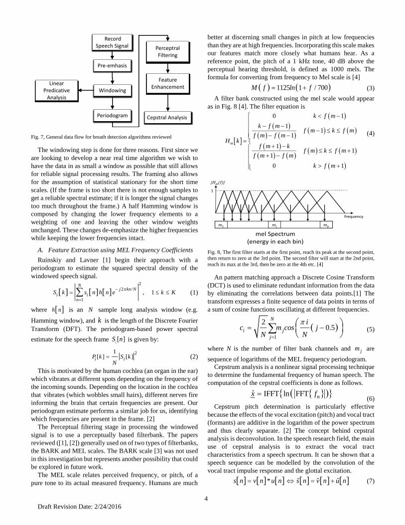
C. Creating Exemplars
Regardless of the approach used, it is necessary to identify a
set of examples or exemplars to be used for training. The
process of building exemplars involves isolating multiple
instances of the air rushing into the mask in the recorded sound
track. These sounds usually are corrupted with the low air alarm
sound which is a clacking noise at approximately 28Hz (Fig. 6).
The regulator inspirational sound with the low air alarm
superimposed was used to form the exemplars.
Fig. 6, The low air alarm is a cyclic sound made with a clacker at approximately
28Hz,
Using a sound mixing tool, the exemplars of the sounds are
isolated and recorded into wave files. Each exemplar recording
is sectioned into 15 ms frames with an overlap 5 ms. The frames
are then windowed with a half-hamming window to smooth
edges and de-emphasize high frequency components. The
windowed frames are pre-emphasized using a first-order
difference filter.
In our implementation of the LPC approach, we used a
shortened exemplar to see if we could develop a measurement
of signal duration as well as measure the time between
inhalations. The shortened exemplars approach did not work as
well for the pattern matching approach. Since the similarity
between consonants, thermal noise and the inhalation noise is
too close to distinguish between the three. The LPC approach’s
real strength is the ability to make this distinction,
IV. FEATURE EXTRACTION/ENHANCEMENT
The general structure of the algorithms is shown in Fig. 7.
The pre-emphasis stage usually involves the removal or
minimization of non-speech sound. The windowing frames the
signal into short time intervals (20 to 40ms wide).
FeatureExtractor
Template or StatisticalClassifier
FeatureVectors
SpeechSignal
Breathing Event
Exemplars
Not a Breathing Event
4
Draft Revision Date: 2/24/2016
Fig. 7, General data flow for breath detection algorithms reviewed
The windowing step is done for three reasons. First since we
are looking to develop a near real time algorithm we wish to
have the data in as small a window as possible that still allows
for reliable signal processing results. The framing also allows
for the assumption of statistical stationary for the short time
scales. (If the frame is too short there is not enough samples to
get a reliable spectral estimate; if it is longer the signal changes
too much throughout the frame.) A half Hamming window is
composed by changing the lower frequency elements to a
weighting of one and leaving the other window weights
unchanged. These changes de-emphasize the higher frequencies
while keeping the lower frequencies intact.
A. Feature Extraction using MEL Frequency Coefficients
Ruinskiy and Lavner [1] begin their approach with a
periodogram to estimate the squared spectral density of the
windowed speech signal.
2
2 /
1
, 1
Nj kn N
i in
S k s n h n e k K
(1)
where h n is an N sample long analysis window (e.g.
Hamming window), and k is the length of the Discrete Fourier
Transform (DFT). The periodogram-based power spectral
estimate for the speech frame [ ]i
S n is given by:
21
[ ] [ ]i iP k S kN
(2)
This is motivated by the human cochlea (an organ in the ear)
which vibrates at different spots depending on the frequency of
the incoming sounds. Depending on the location in the cochlea
that vibrates (which wobbles small hairs), different nerves fire
informing the brain that certain frequencies are present. Our
periodogram estimate performs a similar job for us, identifying
which frequencies are present in the frame. [2]
The Perceptual filtering stage in processing the windowed
signal is to use a perceptually based filterbank. The papers
reviewed ([1], [2]) generally used on of two types of filterbanks,
the BARK and MEL scales. The BARK scale [3] was not used
in this investigation but represents another possibility that could
be explored in future work.
The MEL scale relates perceived frequency, or pitch, of a
pure tone to its actual measured frequency. Humans are much
better at discerning small changes in pitch at low frequencies
than they are at high frequencies. Incorporating this scale makes
our features match more closely what humans hear. As a
reference point, the pitch of a 1 kHz tone, 40 dB above the
perceptual hearing threshold, is defined as 1000 mels. The
formula for converting from frequency to Mel scale is [4]
1125 1 / 700M f ln f (3)
A filter bank constructed using the mel scale would appear
as in Fig. 8 [4]. The filter equation is
0 1
11
1
11
1
0 1
m
k f m
k f mf m k f m
f m f mH k
f m kf m k f m
f m f m
k f m
(4)
Fig. 8, The first filter starts at the first point, reach its peak at the second point, then return to zero at the 3rd point. The second filter will start at the 2nd point,
reach its max at the 3rd, then be zero at the 4th etc. [4]
An pattern matching approach a Discrete Cosine Transform
(DCT) is used to eliminate redundant information from the data
by eliminating the correlations between data points.[1] The
transform expresses a finite sequence of data points in terms of
a sum of cosine functions oscillating at different frequencies.
1
2 0.5
N
i j
j
ic m cos j
N N
(5)
where N is the number of filter bank channels and jm are
sequence of logarithms of the MEL frequency periodogram.
Cepstrum analysis is a nonlinear signal processing technique
to determine the fundamental frequency of human speech. The
computation of the cepstral coefficients is done as follows.
IFFT lˆ F Tn F nx f
(6)
Cepstrum pitch determination is particularly effective
because the effects of the vocal excitation (pitch) and vocal tract
(formants) are additive in the logarithm of the power spectrum
and thus clearly separate. [2] The concept behind cepstral
analysis is deconvolution. In the speech research field, the main
use of cepstral analysis is to extract the vocal tract
characteristics from a speech spectrum. It can be shown that a
speech sequence can be modelled by the convolution of the
vocal tract impulse response and the glottal excitation.
* s n v n u n s n v n u n (7)
Pre-emhasis
Windowing
Record Speech Signal
Periodogram
PerceptralFiltering
Cepstral Analysis
Linear Predicative
Analysis
Feature Enhancement
mjm1 mp
1
frequency
|Hm(f)|
mel Spectrum (energy in each bin)
5
Draft Revision Date: 2/24/2016
where v n is the impulse response of the vocal tract filter;
u n is the glottal excitation, which is usually a quasi-periodic
impulse sequence for voiced speech; s n is the cepstrum of
the speech sequence; v n is the cepstrum of the vocal tract
impulse response sequence; u n is the cepstrum of the glottal
excitation sequence. [2]
Finally a liftering operation is performed to further isolate
and identify the coefficients of interest. The principal advantage
of cepstral coefficients is that they are generally decorrelated
and this allows diagonal covariances to be used in the hidden
Markov models (HMMs). However, one minor problem with
them is that the higher order cepstra are numerically quite small
and this results in a very wide range of variances when going
from the low to high cepstral coefficients, nc . The value L to
lifter the cepstra according to the following formula [5]
12
n n
L nc sin c
L
(8)
Next a matrix is formed by concatenating MFCC vectors for
each subframe. Each such matrix is denoted, by iM where
1, ,i N and N is the number of exemplars used to build
the template.
The DC component is removed by subtracting the mean for
each subframe MFCC vector. An estimate of the unbiased mean
cepstrogram is found by averaging the matrices across the
sample sets:
1
1
i
i
N
T MN
(9)
The variance is estimated using the sample standard
deviations for the cepstrograms:
2
1
1
1ii
i
N
V M TN
(10)
The resulting templates are shown in Fig. 9.
A singular value decomposition (SVD) of the resulting
matrix is computed on the Unbiased MFCCs Template. The
First singular vector (1
S ) corresponding to the largest singular
value is derived. This vector is expected to capture the most
important features of the breath event, and thus, improve the
separation ability of the algorithm when used together with the
template matrix in the calculation of the breath similarity
measure of test signals.
B. Feature Extraction using LPC
In human speech production, the shape of the vocal tract
governs the nature of the sound being produced. In order to
study the properties quantitatively, the vocal tract is modelled
by a digital all-pole filter. [6], [2] The following equation
expresses the transfer function of the filter model in z-domain,
1
1
1N
kk
V z Aa z
(11)
where V z is the vocal tract transfer function. G is the gain
Fig. 9, The resulting mean and variance Templates for the exemplars.
of the filter and { ka } is a set of autoregression coefficients
called Linear Prediction Coefficients. The upper limit of
summation, N, is the order of the all-pole filter. The set of LPC
determines the characteristics of the vocal tract transfer
function. Solving for the LPC involves calculating a matrix of
simultaneous equations xR and the autocorrelation of the
windowed speech frames xxR n .
*0 1
1 0
xx XX
H
x
xx xx
R R N
R E x n x n
R N R
(12)
The following equation is then solved for the autoregression
coefficients.
1 1xx
x
N xx
a R
R
a R N
(13)
The gain of the all-pole filter can be found by solving the
following equation.
1
0N
xx k xx
k
A R a R k
(14)
V. DETECTION CRITERIA
A. Pattern Matching Approach
In the study, the entire file is read in and processed into a
cepstrogram. A sliding window is then passed over the data.
The window is slide to the right by one cepstral column and the
process of computing the breathiness index is performed using
the cepstogram for the data falling inside the window.
The normalized the difference matrix is computed first.
6
Draft Revision Date: 2/24/2016
/i
D M X T V (15)
The normalization by the variance matrix (V ) is performed
element-by-element. Normalizing compensates for differences
in the distributions of the various cepstral columns.
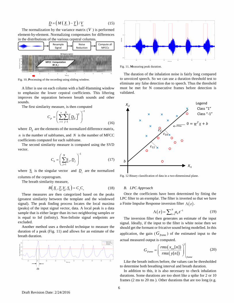
Fig. 10, Processing of the recording using sliding window.
A lifter is use on each column with a half-Hamming window
to emphasize the lower cepstral coefficients. This liftering
improves the separation between breath sounds and other
sounds.
The first similarity measure, is then computed
1
1
2
1
n
i
N
p ij
j
C D
(16)
where ijD are the elements of the normalized difference matrix,
n is the number of subframes, and N is the number of MFCC
coefficients computed for each subframe.
The second similarity measure is computed using the SVD
vector.
1
1
,
N
n i j
j
C S D
(17)
where 1
S is the singular vector and j
D are the normalized
columns of the cepstrogram.
The breath similarity measure,
1, , ,
i p nB X T V S C C (18)
These measures are then categorized based on the peaks
(greatest similarity between the template and the windowed
signal). The peak finding process locates the local maxima
(peaks) of the input signal vector, data. A local peak is a data
sample that is either larger than its two neighboring samples or
is equal to Inf (infinity). Non-Infinite signal endpoints are
excluded.
Another method uses a threshold technique to measure the
duration of a peak (Fig. 11) and allows for an estimate of the
breath duration.
Fig. 11, Measuring peak duration.
The duration of the inhalation noise is fairly long compared
to unvoiced speech. So we can use a duration threshold test to
eliminate any false detection due to speech. Thus the threshold
must be met for N consecutive frames before detection is
validated.
B. LPC Approach
Once the coefficients have been determined by fitting the
LPC filter to an exemplar. The filter is inverted so that we have
a Finite Impulse Response inversion filter z .
1
1
N
kkz a z
(19)
The inversion filter then generates an estimate of the input
signal. Ideally, if the input to the filter is white noise then we
should get the formant or fricative sound being modelled. In this
application, the gain ( frameG ) of the estimated input to the
actual measured output is computed.
2
[ ]
[ ]
est
frame
frame
rms x nG
rms y n
(20)
Like the breath indices before, the values can be thresholded
to determine both breathing interval and breath duration.
In addition to this, it is also necessary to check inhalation
durations. Some durations are too short like a spike for 2 or 10
frames (2 ms to 20 ms ). Other durations that are too long (e.g.
Resample Signal
Noise Reduction
Compute all MFCCs
MFCC Computation
Dt
Fig. 12 Binary classification of data in a two-dimensional plane.
Xi2
Xi1
Class “1”
Class “-1”
Legend
b
7
Draft Revision Date: 2/24/2016
1 minute or more). The method also may classify durations with
minimal power compared to the power level usually present on
the in the regulator inflow.
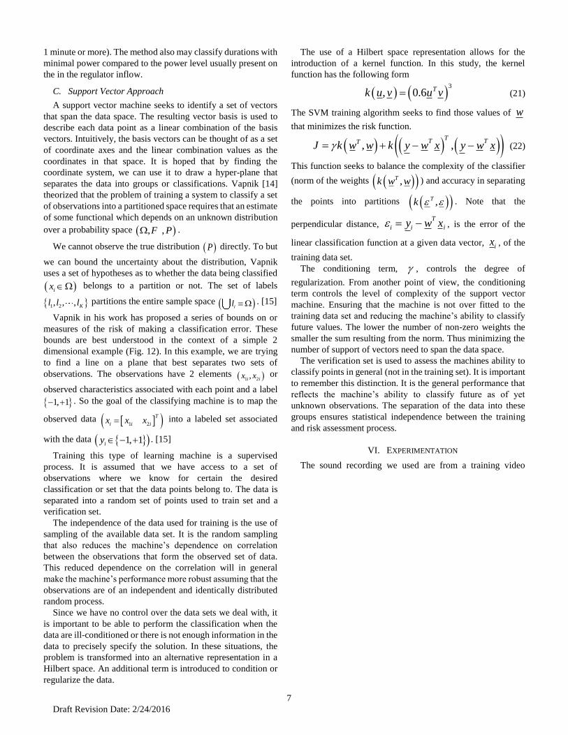
C. Support Vector Approach
A support vector machine seeks to identify a set of vectors
that span the data space. The resulting vector basis is used to
describe each data point as a linear combination of the basis
vectors. Intuitively, the basis vectors can be thought of as a set
of coordinate axes and the linear combination values as the
coordinates in that space. It is hoped that by finding the
coordinate system, we can use it to draw a hyper-plane that
separates the data into groups or classifications. Vapnik [14]
theorized that the problem of training a system to classify a set
of observations into a partitioned space requires that an estimate
of some functional which depends on an unknown distribution
over a probability space , , P F .
We cannot observe the true distribution P directly. To but
we can bound the uncertainty about the distribution, Vapnik
uses a set of hypotheses as to whether the data being classified
ix belongs to a partition or not. The set of labels
1 2, , , Kl l l partitions the entire sample space il . [15]
Vapnik in his work has proposed a series of bounds on or
measures of the risk of making a classification error. These
bounds are best understood in the context of a simple 2
dimensional example (Fig. 12). In this example, we are trying
to find a line on a plane that best separates two sets of
observations. The observations have 2 elements 1 2,i ix x or
observed characteristics associated with each point and a label
1, 1 . So the goal of the classifying machine is to map the
observed data 1 2
T
i i ix x x into a labeled set associated
with the data 1, 1iy . [15]
Training this type of learning machine is a supervised
process. It is assumed that we have access to a set of
observations where we know for certain the desired
classification or set that the data points belong to. The data is
separated into a random set of points used to train set and a
verification set.
The independence of the data used for training is the use of
sampling of the available data set. It is the random sampling
that also reduces the machine’s dependence on correlation
between the observations that form the observed set of data.
This reduced dependence on the correlation will in general
make the machine’s performance more robust assuming that the
observations are of an independent and identically distributed
random process.
Since we have no control over the data sets we deal with, it
is important to be able to perform the classification when the
data are ill-conditioned or there is not enough information in the
data to precisely specify the solution. In these situations, the
problem is transformed into an alternative representation in a
Hilbert space. An additional term is introduced to condition or
regularize the data.
The use of a Hilbert space representation allows for the
introduction of a kernel function. In this study, the kernel
function has the following form
3
, 0.6 Tk u v u v (21)
The SVM training algorithm seeks to find those values of w
that minimizes the risk function.
, ,T
T TTJ k w w k y w wx y x (22)
This function seeks to balance the complexity of the classifier
(norm of the weights ,Tk w w ) and accuracy in separating
the points into partitions ,Tk . Note that the
perpendicular distance, i ii
Txy w , is the error of the
linear classification function at a given data vector, ix , of the
training data set.
The conditioning term, , controls the degree of
regularization. From another point of view, the conditioning
term controls the level of complexity of the support vector
machine. Ensuring that the machine is not over fitted to the
training data set and reducing the machine’s ability to classify
future values. The lower the number of non-zero weights the
smaller the sum resulting from the norm. Thus minimizing the
number of support of vectors need to span the data space.
The verification set is used to assess the machines ability to
classify points in general (not in the training set). It is important
to remember this distinction. It is the general performance that
reflects the machine’s ability to classify future as of yet
unknown observations. The separation of the data into these
groups ensures statistical independence between the training
and risk assessment process.
VI. EXPERIMENTATION
The sound recording we used are from a training video
8
Draft Revision Date: 2/24/2016
(“FIREGROUND Fire Entrapment - Conserving SCBA Air”)
[9] intended to educate firefighters on what to do when their
low air alarm goes off. The tape begins with some music
followed by the training breathing using the SCBA equipment.
He then takes the mask off and lectures. After the lecture he
puts the mask back on and then proceeds to use a stair climber
to simulate doing the labor a fireman does. The low alarm goes
off and the trainer proceeds to review air conservation
procedures with the mask on.
In a near real time application data would be processed as
each frame is completed. However, in this study, the entire file
is read in and processed into a cepstrogram. Then using a sliding
window of the same width as the templates. The window is
advanced or slide to the right by one cepstral column. The
breathiness index computation is then repeated for the data
falling inside the window
.
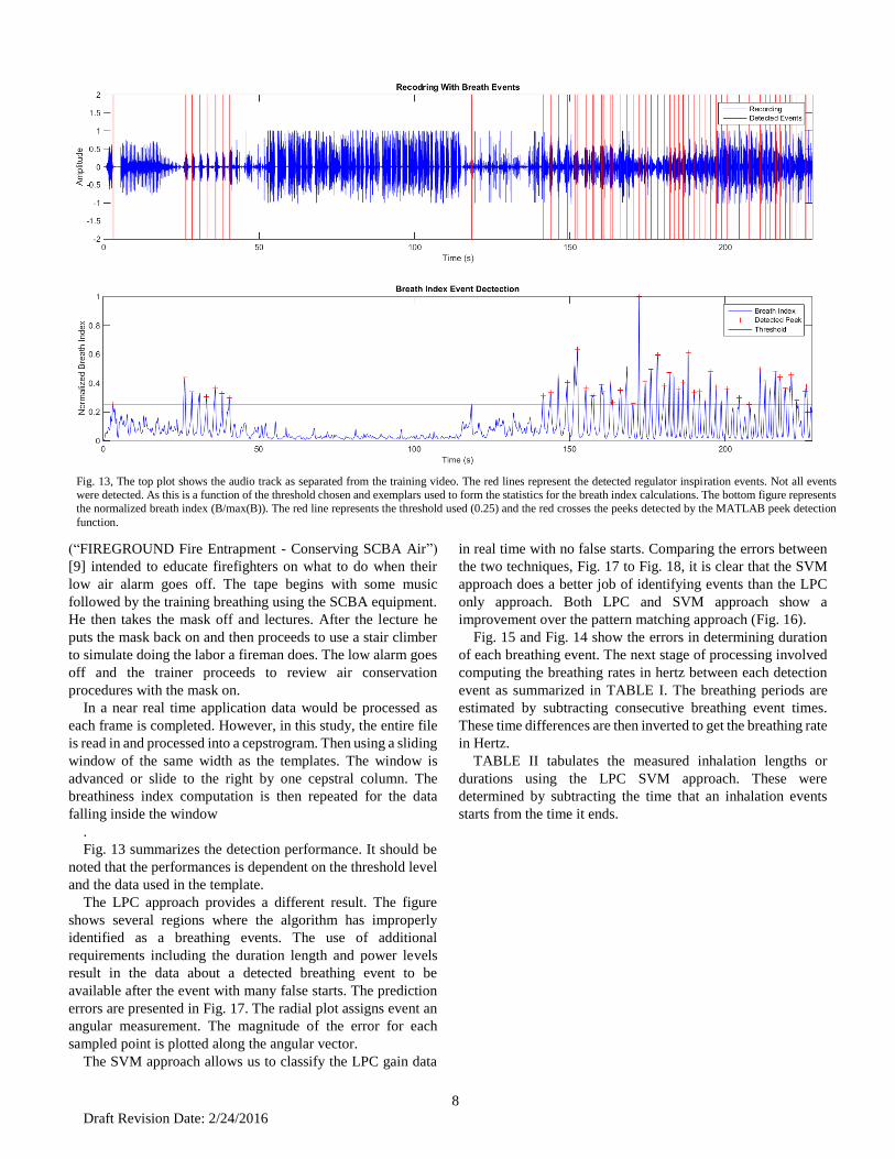
Fig. 13 summarizes the detection performance. It should be
noted that the performances is dependent on the threshold level
and the data used in the template.
The LPC approach provides a different result. The figure
shows several regions where the algorithm has improperly
identified as a breathing events. The use of additional
requirements including the duration length and power levels
result in the data about a detected breathing event to be
available after the event with many false starts. The prediction
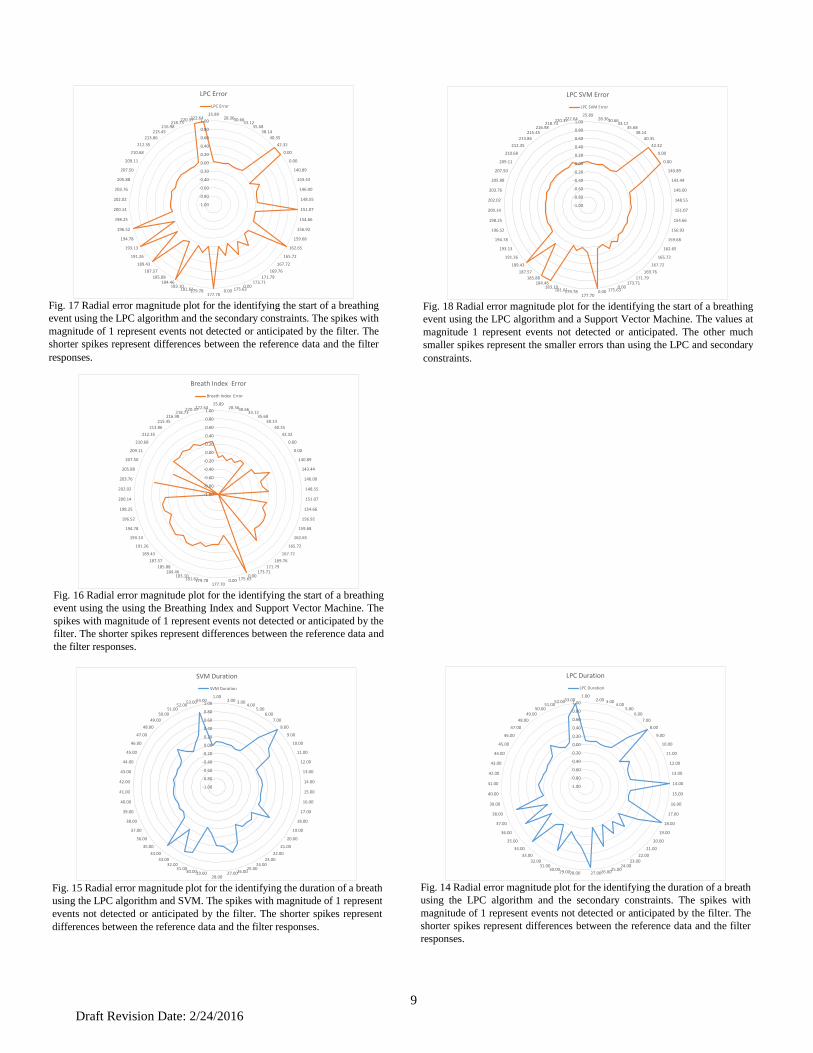
errors are presented in Fig. 17. The radial plot assigns event an
angular measurement. The magnitude of the error for each
sampled point is plotted along the angular vector.
The SVM approach allows us to classify the LPC gain data
in real time with no false starts. Comparing the errors between
the two techniques, Fig. 17 to Fig. 18, it is clear that the SVM
approach does a better job of identifying events than the LPC
only approach. Both LPC and SVM approach show a
improvement over the pattern matching approach (Fig. 16).
Fig. 15 and Fig. 14 show the errors in determining duration
of each breathing event. The next stage of processing involved
computing the breathing rates in hertz between each detection
event as summarized in TABLE I. The breathing periods are
estimated by subtracting consecutive breathing event times.
These time differences are then inverted to get the breathing rate
in Hertz.
TABLE II tabulates the measured inhalation lengths or
durations using the LPC SVM approach. These were
determined by subtracting the time that an inhalation events
starts from the time it ends.
Fig. 13, The top plot shows the audio track as separated from the training video. The red lines represent the detected regulator inspiration events. Not all events
were detected. As this is a function of the threshold chosen and exemplars used to form the statistics for the breath index calculations. The bottom figure represents
the normalized breath index (B/max(B)). The red line represents the threshold used (0.25) and the red crosses the peeks detected by the MATLAB peek detection
function.
9
Draft Revision Date: 2/24/2016
Fig. 17 Radial error magnitude plot for the identifying the start of a breathing
event using the LPC algorithm and the secondary constraints. The spikes with
magnitude of 1 represent events not detected or anticipated by the filter. The
shorter spikes represent differences between the reference data and the filter
responses.
-1.00
-0.80
-0.60
-0.40
-0.20
0.00
0.20
0.40
0.60
0.80
1.00
25.8928.3630.66
33.1235.68
38.14
40.35
42.32
0.00
0.00
140.89
143.44
146.00
148.55
151.07
154.66
156.92
159.68
162.65
165.72
167.72
169.76
171.79173.71
0.00175.630.00
177.70179.78181.61
183.10184.46
185.88
187.57
189.43
191.26
193.13
194.78
196.52
198.25
200.14
202.02
203.76
205.88
207.50
209.11
210.68
212.35
213.86
215.45216.98
218.73220.37222.64
LPC Error
LPC Error
Fig. 18 Radial error magnitude plot for the identifying the start of a breathing
event using the LPC algorithm and a Support Vector Machine. The values at
magnitude 1 represent events not detected or anticipated. The other much
smaller spikes represent the smaller errors than using the LPC and secondary
constraints.
-1.00
-0.80
-0.60
-0.40
-0.20
0.00
0.20
0.40
0.60
0.80
1.00
25.8928.3630.66
33.1235.68
38.14
40.35
42.32
0.00
0.00
140.89
143.44
146.00
148.55
151.07
154.66
156.92
159.68
162.65
165.72
167.72
169.76
171.79173.71
0.00175.630.00
177.70179.78181.61
183.10184.46
185.88
187.57
189.43
191.26
193.13
194.78
196.52
198.25
200.14
202.02
203.76
205.88
207.50
209.11
210.68
212.35
213.86
215.45216.98
218.73220.37222.64
LPC SVM Error
LPC SVM Error
Fig. 16 Radial error magnitude plot for the identifying the start of a breathing
event using the using the Breathing Index and Support Vector Machine. The
spikes with magnitude of 1 represent events not detected or anticipated by the
filter. The shorter spikes represent differences between the reference data and
the filter responses.
-1.00
-0.80
-0.60
-0.40
-0.20
0.00
0.20
0.40
0.60
0.80
1.00
25.8928.3630.66
33.1235.68
38.14
40.35
42.32
0.00
0.00
140.89
143.44
146.00
148.55
151.07
154.66
156.92
159.68
162.65
165.72
167.72
169.76
171.79173.71
0.00175.630.00
177.70179.78181.61
183.10184.46
185.88
187.57
189.43
191.26
193.13
194.78
196.52
198.25
200.14
202.02
203.76
205.88
207.50
209.11
210.68
212.35
213.86
215.45216.98
218.73220.37222.64
Breath Index Error
Breath Index Error
Fig. 15 Radial error magnitude plot for the identifying the duration of a breath
using the LPC algorithm and SVM. The spikes with magnitude of 1 represent
events not detected or anticipated by the filter. The shorter spikes represent
differences between the reference data and the filter responses.
-1.00
-0.80
-0.60
-0.40
-0.20
0.00
0.20
0.40
0.60
0.80
1.00
1.002.00 3.00
4.005.00
6.00
7.00
8.00
9.00
10.00
11.00
12.00
13.00
14.00
15.00
16.00
17.00
18.00
19.00
20.00
21.00
22.00
23.0024.00
25.0026.0027.00
28.0029.0030.00
31.0032.00
33.00
34.00
35.00
36.00
37.00
38.00
39.00
40.00
41.00
42.00
43.00
44.00
45.00
46.00
47.00
48.00
49.00
50.0051.00
52.0053.0054.00
SVM Duration
SVM Duration
Fig. 14 Radial error magnitude plot for the identifying the duration of a breath
using the LPC algorithm and the secondary constraints. The spikes with
magnitude of 1 represent events not detected or anticipated by the filter. The
shorter spikes represent differences between the reference data and the filter
responses.
-1.00
-0.80
-0.60
-0.40
-0.20
0.00
0.20
0.40
0.60
0.80
1.00
1.002.00 3.00
4.005.00
6.00
7.00
8.00
9.00
10.00
11.00
12.00
13.00
14.00
15.00
16.00
17.00
18.00
19.00
20.00
21.00
22.0023.00
24.0025.00
26.0027.0028.0029.0030.00
31.0032.00
33.00
34.00
35.00
36.00
37.00
38.00
39.00
40.00
41.00
42.00
43.00
44.00
45.00
46.00
47.00
48.00
49.0050.00
51.0052.0053.00
LPC Duration
LPC Duration
10
Draft Revision Date: 2/24/2016
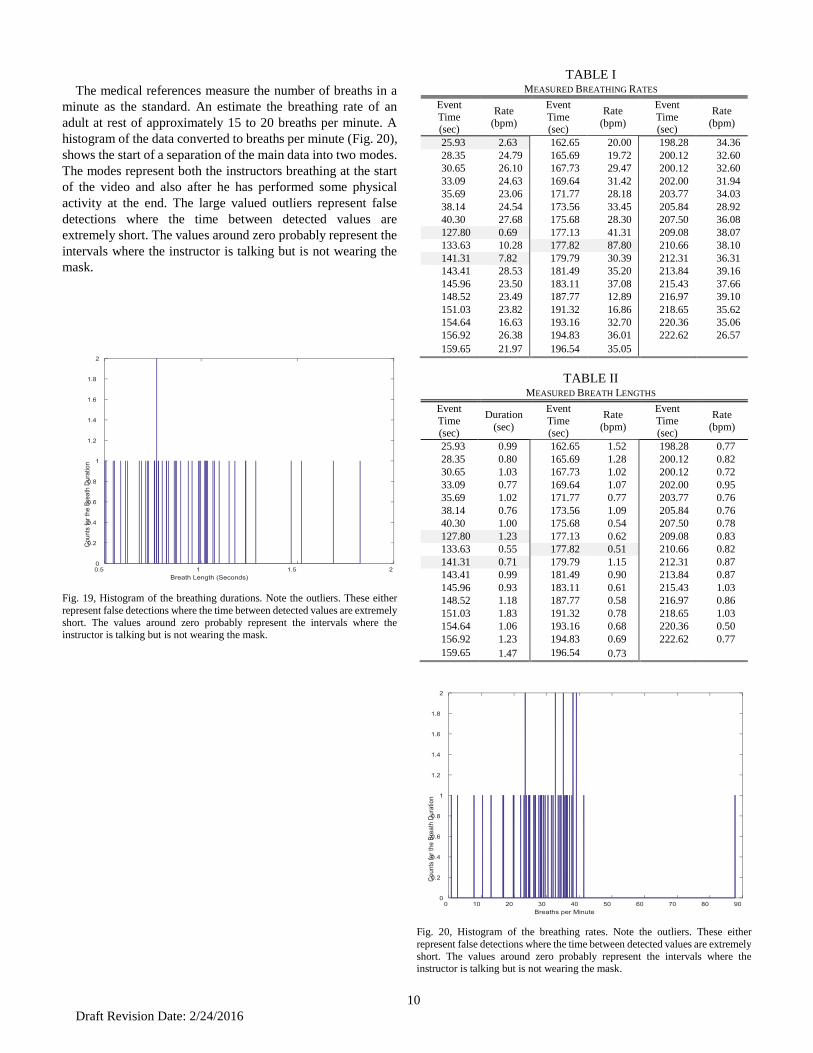
The medical references measure the number of breaths in a
minute as the standard. An estimate the breathing rate of an
adult at rest of approximately 15 to 20 breaths per minute. A
histogram of the data converted to breaths per minute (Fig. 20),
shows the start of a separation of the main data into two modes.
The modes represent both the instructors breathing at the start
of the video and also after he has performed some physical
activity at the end. The large valued outliers represent false
detections where the time between detected values are
extremely short. The values around zero probably represent the
intervals where the instructor is talking but is not wearing the
mask.
Fig. 19, Histogram of the breathing durations. Note the outliers. These either
represent false detections where the time between detected values are extremely
short. The values around zero probably represent the intervals where the instructor is talking but is not wearing the mask.
TABLE I MEASURED BREATHING RATES
Event
Time (sec)
Rate
(bpm)
Event
Time (sec)
Rate
(bpm)
Event
Time (sec)
Rate
(bpm)
25.93 2.63 162.65 20.00 198.28 34.36
28.35 24.79 165.69 19.72 200.12 32.60
30.65 26.10 167.73 29.47 200.12 32.60
33.09 24.63 169.64 31.42 202.00 31.94
35.69 23.06 171.77 28.18 203.77 34.03
38.14 24.54 173.56 33.45 205.84 28.92
40.30 27.68 175.68 28.30 207.50 36.08
127.80 0.69 177.13 41.31 209.08 38.07
133.63 10.28 177.82 87.80 210.66 38.10
141.31 7.82 179.79 30.39 212.31 36.31
143.41 28.53 181.49 35.20 213.84 39.16
145.96 23.50 183.11 37.08 215.43 37.66
148.52 23.49 187.77 12.89 216.97 39.10
151.03 23.82 191.32 16.86 218.65 35.62
154.64 16.63 193.16 32.70 220.36 35.06
156.92 26.38 194.83 36.01 222.62 26.57
159.65 21.97 196.54 35.05
TABLE II MEASURED BREATH LENGTHS
Event
Time (sec)
Duration
(sec)
Event
Time (sec)
Rate
(bpm)
Event
Time (sec)
Rate
(bpm)
25.93 0.99 162.65 1.52 198.28 0.77
28.35 0.80 165.69 1.28 200.12 0.82
30.65 1.03 167.73 1.02 200.12 0.72
33.09 0.77 169.64 1.07 202.00 0.95
35.69 1.02 171.77 0.77 203.77 0.76
38.14 0.76 173.56 1.09 205.84 0.76
40.30 1.00 175.68 0.54 207.50 0.78
127.80 1.23 177.13 0.62 209.08 0.83
133.63 0.55 177.82 0.51 210.66 0.82
141.31 0.71 179.79 1.15 212.31 0.87
143.41 0.99 181.49 0.90 213.84 0.87
145.96 0.93 183.11 0.61 215.43 1.03
148.52 1.18 187.77 0.58 216.97 0.86
151.03 1.83 191.32 0.78 218.65 1.03
154.64 1.06 193.16 0.68 220.36 0.50
156.92 1.23 194.83 0.69 222.62 0.77
159.65 1.47 196.54 0.73
Fig. 20, Histogram of the breathing rates. Note the outliers. These either
represent false detections where the time between detected values are extremely
short. The values around zero probably represent the intervals where the instructor is talking but is not wearing the mask.

11
Draft Revision Date: 2/24/2016
VII. CONCLUSION
The methods studied indicate that an approach like this is
promising but is heavily dependent on having a high energy
signature event being monitored. It is also sensitive to the
threshold values being used. An alternative approach using
wavelets might be able to yield a simpler algorithm for detect
breathing events.
We will continue to refine the process by developing a
machine learning technique/algorithm that will focus on
classifying the breathing rate as normal or an outlier and also to
be able to determine at rest and under stress levels of breathing.
References [1] D. Ruinskiy and Y. Lavner, "An effective algorithm for automatic
detection and exact demarcation of breath sounds in speech and song
signals, " IEEE Transactions on Audio, Speech and Language Processing,
vol. 15, no. 3, pp. 838-850, 2007..
[2] Octavian Cheng, Waleed Abdulla, Zoran Salcic, “Performance
Evaluation of Front-end Processing for Speech Recognition Systems”,
School of Engineering Report No. 621, Electrical and Computer
Engineering Department, School of Engineering, The University of
Auckland
[3] Zwicker, E., Terhardt, E.: “Analytical expressions for critical-band rate
and critical bandwidth as a function of frequency.” J. Acoust. Soc. Am.
68, 1523–1525 (1980)
[4] Rabiner, L., Juang, B.H., Fundamental of Speech Recognition. Prentice-
Hall, Upper Saddle River (1993)
[5] S. Young, J. Odell, D. Ollamson, V. Valtchev, P. Woodland, “5.3 Linear
Prediction Analysis” from The HTK Handbook,
http://www.ee.columbia.edu/ln/rosa/doc/HTKBook21/node54.html
[6] Thomas Quatieri, Discrete-time Speech Signal Processing: Principles
And Practice, Prentice Hall Press, Upper Saddle River, NJ, USA ©2001
[7] A. Michael Noll (1967), “Cepstrum Pitch Determination,” Journal of the
Acoustical Society of America, Vol. 41, No. 2, pp. 293-309
[8] Oppenheim, A.V., and R.W. Schafer. Discrete-Time Signal Processing.
Englewood Cliffs, NJ: Prentice Hall, 1975, Section 10.5.3.
[9] “Fire Entrapment - Conserving SCBA Air” from
http://www.firerescue1.com/videos/originals/fireground/1479446-
FIREGROUND-Fire-Entrapment-Conserving-SCBA-Air/
[10] Kamil Wojcicki, HTK MFCC MATLAB,
http://www.mathworks.com/matlabcentral/fileexchange/32849-htk-
mfcc-matlab/content/mfcc/mfcc.m, September 2011
[11] Mike Brookes, “VOICEBOX, a MATLAB toolbox for speech
processing”,
http://www.ee.ic.ac.uk/hp/staff/dmb/voicebox/voicebox.html
[12] Ahmad Abushakra and Miad Faezipour, “Acoustic Signal Classification
of Breathing Movements to Virtually Aid Breath Regulation” IEEE
Journal Of Biomedical And Health Informatics, VOL. 17, NO. 2,
MARCH 2013
[13] William M. Kushner S. Michelle Harton and Robert J. Novorita, The
Distorting Effects Of SCBA Equipment On Speech And Algorithms For
Mitigation, 13th European Signal Processing Conference (EUSIPCO
2005) Proceedings, pp. 576-580
[14] V. Vapnik. Estimation of Dependences Based on Empirical Data [in
Russian]. Nauka, Moscow, 1979. (English translation: Springer Verlag,
New York, 1982).
[15] Christopher J.C. Burges, A Tutorial on Support Vector Machines for Pattern Recognition, Data Mining and Knowledge Discovery 2, 121-167,
1998 Basic format for periodicals:
[16] Rui Carlos Sá, Yves Verbandt, “Automated Breath Detection on Long-Duration Signals Using Feedforward Backpropagation Artificial Neural
Networks”, IEEE Transactions on Biomedical Engineering, 2002,
49(10), p 1130-1141. [17] Cheng Li; Parham, D.F.; Yanwu Ding “Cycle Detection In Speech
Breathing Signals” Biomedical Sciences and Engineering Conference (BSEC), 2011 Year: 2011 Pages: 1 - 3, DOI: 10.1109/
BSEC.2011.5872314
[18] P. J. Price, M. Ostendorf, and C. W. Wightman, "Prosody And Parsing"
Proceedings of the workshop on Speech and Natural Language, pp. 5-11, 1989.
[19] W. Wightman and M. Ostendorf, "Automatic Recognition Of Prosodic
Phrases", Proceedings of the International Conference on Acoustics, Speech and Signal Processing, ICASSP, pp. 321-324, 1991.
[20] T. Nakano, J. Ogata, M. Goto, and Y. Hiraga, "Analysis And Automatic
Detection Of Breath Sounds In Unaccompanied Singing Voice," Proceedings of the 1Oth international Conference on Music Perception
and Cognition, pp. 387-390, 2008.
[21] G. Tzanetakis and P. Cook, "Audio information retrieval (air) tools," Proc. Int. Symposium on Music Information Retrieval (ISMIR), 2000.
[22] S. Borys and M.Hasegawa-Johnson ”Recognition Of Prosodic Factors
And Detection Of Landmarks For Improvements To Continuous Speech Recognition Systems” Undergraduate Thesis, Bachelor of Science in
Electrical Engineering in the College of the University of Illinois at
Urbana-Champaign, 2004 [23] M. Igras, B. Ziolko, “Wavelet Method For Breath Detection In Audio
Signals”, Multimedia and Expo (ICME), 2013 IEEE International
Conference on Year: 2013 Pages: 1 - 6, DOI: 10.1109/ ICME.2013.6607428
[24] H. Sakoe and S. Chiba, "Dynamic programming algorithm
optimization for spoken word recognition," IEEE Transactions of
Acoustics, Speech and Signal Processing, vol. ASSP-26, no. 1, 1978