Erosion risk 1napping; a Dlethodological case study in the

Colo111bian Llanos

Anton Vrieling Version 8131/99

Colombia Wageningen Agricultura! University (WAU)

The Netherlands

lntroduction. ............................................................................................................................................................ 3 Setting ....................................................................................................................................................................... 5

Study area ............................................................................................................................................................. 5 Cümatic properties ............................................................................................................................................. 5 Geology ................................................................................................................................................................. 5 Soils ....................................................................................................................................................................... 5 Vegetation and land use .................................................................................................................................... 5

Materials and methods ......................................................................................................................................... 6 Satelüte images ................................................................................................................................................... 6 Grounddata ......................................................................................................................................................... 6 Digital Elevation Model .................................................................................................................................... 6 Soil data ........................................................................................... .. ................................................................... 6 Software ................................................................................................................................................................ 6

Processing of the Landsat images ...................................................................................................................... 8 Classijication ....................................................................................................................................................... 8 Estimating the vegetative ground cover ........... .. ............................................................................................ 9

Tbe Universal Soil Loss Equation (USLE) ............................................................. ....................................... 11 Rainfall and runoff factor .................................. .. .......................................................................................... 11 The soil erodibiüty factor ................................................................................................................................ 11 The slope fllctors ............................................................................................................................................... 12 The cover and managemenl factor ............................................................................................................... 12 The conserva/ion practice factor ............................................................... .................................................... 12

Tricart Ecodynamic Approach ........................................................................................................................ l3 Results ..................................................................................................................................................................... 15

Classijiclltlon ..................................................................................................................................................... 15 Estimation ofthe vegetative ground cover .................................................................................................. 18 USLE ................................................................................................................................................................... 19

Conclusions/Discussion .............................................................. ........................................................................ 23 References .............................................................................................................................................................. 25 Aone.x 1: [maps-image453.doc] .......................................................................................................................... 28 Aone.x 2: Soil nomograpb for USLE K-factor .............................................................................................. 29 Aone.x 3: Qualifications for Tricart' s Ecodynamic Approacb ................................................................ 30 Aone.x 4~ Determination of tbe Tricart sub factors for tbe present element combinations ............. 31 Aone.x 5: [maps-Landsat products.doc) ............................................................................................................ 32 Anne.x6: [maps-USLE_KLS.doc] ...................................................................................................................... 33 Anne.x 7: [maps-USLE_C.doc] ........................................................................................................................... 34 Aone.x 8: [maps-Tricart Soil and Geology.doc ). ................................. ............................................................. 35 Anne.x9: [maps-Tricart Relief and Vegetation.doc]. ...................................................................................... 36

Introduction

Accelerated soil erosion caused by water is an increasing global problem. Erosion can be defined as the detachment or entrainment of soil particles (Mutchler et al., 1988). Soil erosion by water can be divided into: splash erosion, which occurs when soil particles are detached and transported as a result of the impact falling raindrops, sheet erosion, that removes soil in layers and is caused by the combined effects of splash erosion and surface runoff, ril/ eros ion , which is the disappearance of soil particles caused by concentrations of tlowing water, and gully erosion, that occurs when the concentrations are larger (Stroosnijder and Eppink, 1993). These processes reduce the soil resource, thereby negatively affecting the agricultura} production and sustainability.

Factors wbich control erosion are (Morgan, 1986): l. Climatic characteristics: rainfall volume and intensity 2. Soil properties: soil texture, organic matter content, infiltration capacity, etc. 3. Land management: type ofland use, vegetation cover, etc. 4. Topographical factors: slope steepness and slope length

These factors can be highly variable over space and time. This makes soil water erosion a very dynamic and spatial phenomenon (Hofierka and ~úri, 1996) and thus quantitative erosion mapping a complicated task. However, for land use and conservation planning an analysis of the erosion risk is important.

Such an analysis demands geographically bound data. The data requirement depends on the methodology that is being used for the erosion mapping. Different methodologies exist to infer erosion risks from the available data.

One of the most applied erosion models throughout the world is the Universal Soil Loss Equation, USLE (Wischmeier and Smith, 1978). The USLE is a statistically calibrated model based on data of the erosion controlling factors as collected in the United S tates. A point of criticism made by Tricart and KiewietdeJonge ( 1992) is that the USLE is a simple addition of parameters and thus excludes all interaction and feedback effects in the erosion process, which invalidates its universal use. They pledge for a more qualitative approach in mapping erosion risks. While a quantitative approach is necessary for the design of hydraulic infrastructure such as reservoirs, a qualitative approach is usually suitable for land use and conservation planning purposes.

This study will examine a more qualitative approach. This is the Tricart' s Ecodynamic Approach. This approach is concemed with the various processes and mechanisms that cause changes in the ecological environment, as well as their interactions (Tricart and KiewietdeJonge, 1992). It is applied in a raster environment, where erosion-controlling factors are defined on a raster basis.

Remote sensing can serve as a useful tool in both methods. lt offers fast and cost effective measurements over large areas (Pilesjo, 1992). Especially when other data is not available or hard and costly to acquire, satellite images in the optical and microwave domains can provide helpful data on 1and use, land cover and landforms, which belp to infer erosion risks.

Erosion risks can be divided into potential and actual soil erosion risk. Potential soil erosion risk is defined as the inherent risk of erosion irrespective of current land use or vegetation cover. This potential risk represents the worst situation that might be reached. Actual erosion risk relates to the current risk of erosion under present vegetation and management conditions.

The following study forms part of a land evaluation and land use planning program, that is

executed by CIA T for the Meta department in the Llanos Orientales of Colombia. Last year the emphasis has been on the farm level, this year on the municipality level and next year on the department level. The resulting erosion risk map of this study will be used as input in the land use planning process. The evaluated methodologies will be transferred to the municipalities as the final aim of the CIA T program consists in making the municipalities capable of executing their own land use planning program. Puerto López serves as a pilot municipality.

The first aim of this study is to establish which methodology is most suitable to qualitatively map soil eros ion risk areas in CIA T' s savanna ecoregional test si te, the Puerto López municipality. To attain that purpose, the two methodologies will be studied and applied to the test site. Limitations and advantages of each one will be established. Secondly, this study aims at evaluating which method allows to best take advantage of the information available from the Landsat TM images available for the area.

To reach these purposes, the study can benefit from a digital elevation model, a soil map, a classified 1996 Landsat TM image anda 1998 Landsat TM image.

Setting

Studyarea Puerto López is a municipality in the department of Meta in Colombia. Its geographical position is between 3°40' and 4°27' northem latitude and 72°04' and 73° 15' westem longitude. The municipality has a surface of 6907 km2 and about 24.000 inhabitants of which ll.OOO live in rural areas (CORPOICA, 1995). The height varies between 180 to 300 meters above sea level. The hydrologic system belongs to the Orinoco-watershed and to tbe sub­watershed ofthe Meta-river.

C/imatic properties The region has an average temperature of 27 oc and an annual precipitation of 2.800 mm. The rain mainly falls between April and November, with the highest rainfall in June. This season is called winter. The rainwater increases the discharge ofthe river, which results in the rainy months in inundations (IGAC, 1991 ). The relative humidity varíes between 65% in summer and 90% in winter (Correa et al., 1988). The rainfall regirne creates a high erosion hazard (Restrepo and Navas, 1981 ).

Geology Puerto López is situated in the region that is called the Uanos Orientales, which extends from the Amazons in the south, the Eastem Cordillera of the Andes in the west, and Venezuela in the north and the east The geology of the Uanos Orientales is closely related with the geology of the Bastero Cordillera: the sediments in the Uanos originate from the erosive processes that the mountain range has experienced. Later these sediments were affected by tectonic movements that greatly modified the original sedirnentation pattems (IGAC, 1978). At present, the municipality consists of a low part where the main rivers run that are called alluvial terraces and a higher part that is called the 'altillanura' (high plains). This 'altillanura' can be divided in a not dissected anda dissected part.

Soils The most com.mon soils in the municipality, according to the F AO-classification. are acrisols, ferralsols, cambisols, tluvisols and gleysols. The organic matter content is generally low (Hoyos et al ., 1992), as well as the infiltration capacity. Rainfall ofmore than 20 mm causes runoff and erosion (Amézquita and Londoño, 1997). This low capacity results from a poor structure or a laminar structure, where hardly any macro-pores are present.

V egemtion and Úllfd use The greatest part of the municipality consists of natural and introduced pastures. Cattle breeding forms the prime economic activity in the municipality. The introduced pastures consist of various forms of the species brachiaria; brachiaria decumbens, brachiaria humidicola and brachiaria dictionebra are tbe most present Natural pastures are often subject to bwni.ng, which is done to renovate the pastures and in this way improving the quality of the cattle food. These natural pastures can contain bushes or trees, especially at the transition to forest. Forest occupies another great part of the municipality and the bulk of it is situated around the drainage network, containing a variety of species. Crops and plantation form a relative small part of the area. In the western part of the municipality, rice is an important cash crop, which is grown on large areas and fwnigated by little airplanes. The otber trees and crops cultivated are fruit trees, rubber, plantain, maize, cassava and a few others. Apart from sorne minor cultivations, these can be found around the farm houses.

Social The biggest part of the farm owners doesn ' t live in the municipality, but in cities like Bogotá. They attract people to put in charge of their farms. Usually these encharged people don't stay for a long time at the farm and often lack a good knowledge about the specific qualities of its belonging fields.

Materials and methods

Satellite images

Lanclsat Thematic Mapper (TM) images were used in this study. The Landsat TM is a satellite sensor that records data in 7 different bands. Bands are wavelength filters through which the sensor collects its data. Each band has its own set of data that is stored in 8-bit format This means that the brightness values for each pixel range from O to 255, where O is the darkest value. The spatial resolution ofthe bands is 30 meters, with the exception ofband 6, which has a resolution of 120 meters. The spectral bands are given in table l.

Band Spectral Range l 0.45 - 0.52 J.lm (blue) 2 0.52 - 0.60 J.lm (green) 3 0.63 - 0.69 J.lm (red) 4 0.76 - 0.90 J.lm (near IR) 5 1.55 - 1.75 J.lm (mid IR) 6 10.4 - 12.5 J.liD (thermal) 7 2.08 - 2.35 J.lm (mid IR)

Table 1: Spectral bands for Landsat TM

In this study a Landsat TM image of the · ¡ orh of August 1998 was used. It covers almost the entire municipality, except for a small fringe in the eastem part. Several clouds were present, which made the processing of the image more difficult. A composite of the image can be seen in annex l. Apart from this image, a classified image ofthe fjh ofJanuary 1996 was available

Grounddata

Ground data was collected in June 1999 using a Global Position System (GPS). With the GPS coordinates of the borders of parcels or other bomogeneous areas were measured, wbicb resulted in a collection ofpolygons. For each polygon the land use was determined as well as the average vegetative ground cover. Apart from these data, ground data of March 1998, collected by N. Beaulieu and P. Hill was available.

Soil data

The Colombian geograpbical institute 'Agustín Codazzi' (IGAC) has done a soil study in 1978 for the northeast and central part of the department of Meta, in which the Puerto López municipality is situated (IGAC, 1978). For this soil study, aerial photographs have been used as a base to separate the general landscape forros. Field cbecking and the integration of elements like relief, drainage pattems and land use resulted in the cartographic units for the soils. In these units, pilot zones have been established where a thorough soil study was executed. The results were extrapolated to the whole area. The resultíng map is on a scale l : 100.000. The study is well documented and for each cartographic unit the constitutíng profiles are described in terms of their pbysica1 and cbemical properties. In the Puerto López municipality 19 different cartographic units were defined, of wbicb sorne are subdivided for varying slope classes. Most units have an intemal variability as they consist of 2 or more soil types with different characteristics. The soil map was digitized and the vectors were rasterized to make the map compatible witb the other information.

Digital E/evation Model

The term Digital Elevation Model (DEM) is used to refer to a digital representation of a topographic surface (Felicísimo, 1994). lt contains surface elevation values for regular grid

points. The DEM used in this study was interpolated from elevation contour lines and point elevation data. It has a 25-meter grid. lt can be used to derive topographic parameters, such as slope, slope length and drainage pattem.

Software

The Canadian software package PCI version 6.3 was used on a Windows NT 4.0 workstation to treat the data in this study. PCI is a GIS (Geographical Information System) software package, which is mainly designed to treat raster (satellite or DEM) data, but can also handle vector data. ACE (Advanced Cartographic Environment) version 3.0 by PCI Carto was used to mak:e the maps.

Processing of the Landsat images

Classifteation

In the study area different land cover types are present It is important to define the location of the severa! types as they vary in their effect on the erosion process. Landsat TM irnages forro an important source to derive information on the present land coverage.

Different cover types retlect varying amounts of energy in a single spectral band and a single cover type retlects varying amounts of energy as a function of wavelengtb (Hoffer, 1984). The relation between the energy reflected of an object and the wavelengtb is called the spectral signature of the object For each object class, the reflection can show deviational behavior in each band. The mean reflection of a class and its standard deviation for each band can be used to distinguish it from other classes. This allows multispectral scanners like Landsat TM to be a useful too! in mapping cover classes. Each class has to meet two conditions:

l . The class must be spectrally separable from al1 other classes 2. The class must be of interest to the user or have informational value (Hoffer,

1976)

Two broad classes of classifícation procedures exist for classif)ring remote sensing data. One is referred to as unsupervised classifícation and the other supervised classifícation. Unsupervised classifícation is a method, which examines a large number of unknown pixels and divides them into a number of classes based on their spectral separability. Afterwards these classes can be identified by associating a sample of pixels in each class with available reference data (Richards, 1993). However, a priori analyst information cannot be implemented, which causes that the classes do not always meet the second condition (see above).

Therefor, the supervised classification procedure was considered more appropriate in this study. This method first determines the spectral signatures ofthe training data. Training data are collections of prototype pixels identified in an image, that define the class signatures. The analyst collects this data for al1 desired classes, labels it and trains the classifícation algorithm to recognize the spectral characteristics of each class. This data can be collected in the field, from maps, from aerial photographs or interpreted from the image itself. When trained, the algorithm assigns labels to al1 of the image pixels by using the class estimates.

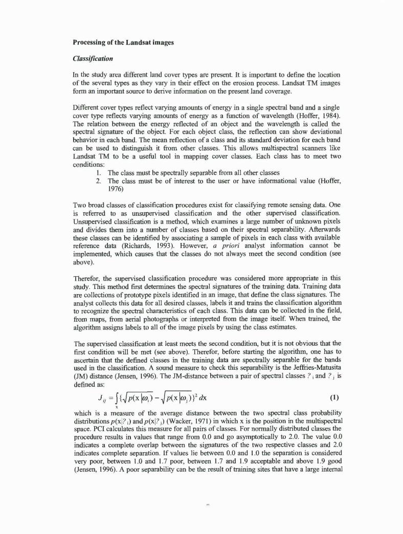
The supervised classifícation at least meets the second condition, but it is not obvious that the fírst condition will be met (see above). Therefor, before starting the algorithm, one has to ascertain that the defined classes in the training data are spectrally separable for the bands used in the classification. A sound measure to check this separability is the Jeffries-Matusita (JM) distance (Jensen, 1996). The JM-distance between a pair of spectral classes ? ; and ? i is defined as:

(1) X

which is a measure of the average distance between the two spectral class probability distributions p(xj? ;) andp(xj? i) (Wacker, 1971) in whicb x is tbe position in the multispectral space. PCI calculates this measure for all pairs of classes. For normally distributed classes the procedure results in values tbat range from 0.0 and go asymptotically to 2.0. The va1ue 0.0 indicates a complete overlap between the signatures of the two respective classes and 2.0 indicates complete separation. If values lie between 0.0 and LO the separation is considered very poor, between 1.0 and 1.7 poor, between 1.7 and 1.9 acceptable and above 1.9 good (Jensen, 1996). A poor separability can be tbe result oftraining sites that have a large interna!

variability within each class. In this case a possibility is to edit the training sites or merge poorly separable classes.

When the separability between the classes is considered acceptable, the supervised classification procedure can begin. The most common supervised classification algorithm is the one of the maximwn likelihood classification. The basis of this method is that a point x in the multispectral space with co-ordinates defined by the brightness values, obtains a probability p(? ;~) that gives the likelihood that the correct class is ? ; for a point at position x , where i takes the value of 1 to the total nwnber of classes. Classification is performed according to:

if for a1J j ~i (2)

This means that the pixel at x belongs to class ? 1 if p(? ~~) is the largest. The probabilities can be calculated from the training data. This is approach is called Bayes' classification (Ricbards, 1993). It is possible to apply thresholds to this approach as a maximum allowable deviation from the mean spectral signatwe. If the probability of a pixel is below the threshold for a certain class, it will not be classified as belonging to that class. The maximwn likelihood classifier is considered to give accurate results when assumed that classes in the input data have a Gaussian distribution.

After the classifi.cation has been performed, its accuracy has to be determined in order to attach a degree of confidence to the results obtained. Preferably this is done with other data than the sites used for training, as these training sites are biased in the classification (Jensen, 1996). This new ground data will be evaluated against the classification map in a confusion matrix (see table 3, page16). This is a square array of nwnbers laid out in rows and columns that expresses the number of sample pixels assigned to a particular class relative to the actual class as verified in the field. The columns represent the ground truth data, while the rows indicate the classification result for the respective pixels. The probability of a reference pixel being correctly classified can be determined by dividing the number of correct pixels in the class by the total nwnber of pixels in the class as derived from the ground truth data (the colwnn total). This measure is called the producer's accuracy. Overall accuracy could be determined by dividing the total correct by the total nwnber of pixels. However, in this study it was assumed that if a large part of the ground truth data fall within one or a few classes, the overall accuracy would be biased. Therefor an adapted overall accuracy was used, that weigbs the respective producer' s accuracy according to percentage occupied by each class in the municipality, which was determined from the classification.

Est/mating the vegetative ground cover

Although the classification gives an indication of which land cover type can be expected on which location, it is also important to know to what extent the soil is covered by the vegetation This influences the susceptibility to soil detachment, mainly through raindrop interception.

Spectral vegetation indices can be related to vegetation cbaracteristics like ground cover percentage. The rationale for these indices is to exploit the unique spectral signature of green vegetation as compared to spectral signatures of other materials. Most vegetation indices are based on the relation between the red and near-infrared retlectance (for Landsat TM bands 3 and 4). The red reflectance is low for vegetation, whereas its near-infrared reflectance is high (figure l).

0.5

8 0.4 e: • ~ 0.3 r:: f 0.2

0.1

1

-dry soil 1 ____ ~r----~-----------1 - green crop

o~~~~~l_~--~~ 0.4 0.5 0.6 0.7 0.8 0.9

wavelengtb (10"'-6 m)

A common used vegetation index is the Normalized Difference Vegetation Index (NDVI). The NDVI is calculated as follows (Rouse et al., 1974):

NDVI = nir -red

where mr red

nir +red = reflectance in the near-infrared band (band 4 for Landsat TM) = reflectance in the red band (band 3 for Landsat TM)

(3)

Its values range from - l to l , but for vegetation and soil these values lie between O and l. The NDVI values can be scaled between the minimum (bare soíl) and maximum ground cover. Scaled NDVI (NI) is defined as:

No= NDVI-NDVI0 ( 4) NDVIs - NDV/0

where NDVIo corresponds to the NDVI values for bare soil and ND\'4 relates to a surface with a vegetation cover of lOO%. An important advantage ofthis scaling is that atmospheric correction of the scaled NDVI is unnecessary for determíning vegetative ground cover, for both clear and hazy conditions (Carlson and Ripley, 1997). However, clouds cause problems in calculating the NDVI, which are not solved by scaling.

Vegetative ground cover (VGC) can be assessed by relating field estimations to the calculated scaled NDVI for the same area. Choudbury et al. ( 1994) and Gillies and Carlson ( 1995) obtained a square root relation between N' and VGC, which can be formulated:

VGC<== N°2

(S) However, a theoretical basis for this relationship does not exist.

The Universal Soil Loss Equation (USLE)

The most widely used prediction equation for average annual sheet and rill erosion is the USLE (Wischmeier and Srnith, 1978). lt is the statistical swnmary of more than 1 O 000 plot­years of data collected on natural runoff plots in the eastern USA. The equation reads:

A = R*K*L * S*C*P in whicb:

A R K L S e p

= the average annual soil loss = the rainfall and runoff factor = the soil erodibility factor = the slope length factor = the slope gradient factor = the cover and management factor = the conservation practice factor

The rainfaU and runofffactor

(t ba-1 y"l ) (MJ ba-1 mm h-1 y"l) (t MJ1 h rmn"1

)

(-) (-) (-) (-)

(6)

The erosive force of the local rainfall regime (the erosivity) is represented by the rainfall factor. The product of kinetic energy and rainfall intensity gives a good representation of this erosivity. The R factor can be calculated as (F oster et al. 1981 ):

where em 130

p j

em=O.ll9+0.0873log(/30 *2) (7) n

R = I)em(/30 *2)p )¡ (8) j"'l

= kinetic energy (MJ ha-1 mm"1) = maximum intensity in 30 min. (mm b"1) = precipitation per shower occurrence (mm) = number of shower occurrences from 1 to n, n being the total yearly number of shower occurrences

However, to apply this equation detailed clirnatic data is needed. This data could not be obtained within the Puerto López municipality. In a neighboring municipality an erosivity study has been done using climatic data for two sequential years 1979 and 1980 (Restrepo and Navas, 1982). They obtained a val u e of 1600 to 1700 MJ ha -l mm li 1 y" 1. Furthermore an isoerodent map, showing lines of equal rainfall erosivity, was available for the whole of Colombia ata scale 1: 3.400.000 (IGAC, 1988). This map shows that the municipality lies in a zone with erosivity between 1500 and 3000 MJ ha-1 mm li1 y"1. Taking into account the location of the neighbouring municipality and the transition to other zones in the map, a value of2000 MJ ha-1 mm h-1 y"1 was considered an acceptable estímate for the municipality. Given the available data the same value was applied for the total area.

The soü erodibility factor This factor quantifies the cohesive, or bonding character of a soil type and its resistance to dislodging and transport dueto raindrop impact and overland flow. It can be linked to the soil properties through the soil erodibility nomograph (Wischmeier et al., 1971 ), sbown in annex 2. This nomograph uses the following inputs:

l. Percentage silt and very fine sand ( 2 - 100 ¡..un) 2. Percentage sand ( > 100 ~) 3. Percentage organic matter 4. Class for soil structure 5. Permeability class

The output is the soil erodibility in English units. This value can be converted to the metric system through multiplication with 1.292.

Classes of soil structure Permeability classes 1 Very fine granular 1 Rapid 2 Fine granular 2 Moderate to rapid 3 Medium or coarse granular 3 Modera te 4 Blockv. platy, or massive 4 Slow to moderate

5 Slow 6 Verv slow

Table 1: Classes for soll structure and permeablllty In the soil erodlblllty nomograpb

In the soil study available, the very fine sand fraction was not determined. Therefor an asswn:ption had to be made. According toE. Amézquita (personal communication, 7/99), it is realistic to assume that 20 percent of the sand fraction of the soils in tbe area consists of very fine sand. The structure class ofthe present soils is either 3 or 4. Structure class 3 was related with a slow permeability, structure class 4 was related witb a very slow permeability.

The slope factors The effects of topography and hydrology on soil loss are characterized by the combined LS factor. According to Wischmeier and Smitb ( 1978), the LS factor is calculated as follows:

LS = (Lj72.6) m * ( 65.41 sin 2 S+ 4.56sin S+ 0.065) (9) where Lis the slope length (feet), S is the degree ofslope and

m= 0.5 if S= 5.0 % m= 0.4 if 3.5 % = S < 5.0 % m= 0.3 if 1.0 % = S < 3.5 % m = 0.2 if S < 1.0 %

Are Macro Language (AML) programs provided by Hickey et al (1994) have been used to calculate the LS-factor within Arc/INFO Grid. Basically, the LS AML takes a DEM, establishes the high points, then, following tbe flow direction, calculates a cumulative LS value down tbe slope. The user inputs a value for the minimum slope change required to cause deposition. This value was set at 0.5 %. The program is iterative and nms a number of times on the entire grid. To test the program a standard plot was constructed with a slope length of 22.1 m and a slope of9% anda grid spacing ofO.lO m. At the bottom ofthe slope the LS-factor should result in a value of 1.0. As this was the case, it was concluded that the program functioned well.

The cover and management factor The cover and management factor is defined as the ratio of soil loss from an area with a specified cover and management to that from an identical area of tilled continuous fallow. lt is an important factor, because it represents conditions that can most easily be managed to reduce erosion (Renard et al., 1994). The standard C-value is a weighted average of seasonal cover-management factor values. Remote sensing offers the possibility to assess the C-factor for extended areas. Pi1esj6 (1992) estimated the C-factor for Ethiopia and Sudan using a relation between Landsat bands 4 and 7. De Jong (1994) related the C-factor to the NDVI for the Mediterranean area. However, most spatial USLE studies using satellite data, perform a classification before determining C-values (Folly et al., 1996; Jürgens and Fander, 1993). This seems more justified as the effects of canopy on soil splash vary among crops, depending on foliage characteristics, canopy beight and ground cover percentage (La1, 1990). C-values for different land cover types can be found in literature.

The conservatwn practice factor A specific support practice, like contouring or contour strip cropping, can reduce the soilloss. This is accounted for in the conservation practice factor. As in the municipality hardly any support practices were encountered, this factor was fixed to 1.0. It remains to be said though that a few farmers practice contouring, although only on sorne of the small cultivated plots. This was considered too insignificant to take into account in this study.

Tricart Ecodynamic Approach

Ecodynamics is the dynamics of the ecological environment (Tricart and KiewietdeJonge, 1992). It is concemed with the various processes and mechanisms that cause changes in the ecological environment. For erosion studies, these processes can be divided into morphogenic processes and pedogenic processes. Morphogenic processes are the processes that form the landscape due to gravitational force or other tangential working forces. Pedogenic processes refer to the development of soil horizons paral1e1 to the soil surface. Morphogenesis generally proceeds down a topographic surface, whereas pedogenesis proceeds vertically.

The morphogenic-pedogenic balance studies the relation of morphogenic to pedogenic mechanisms. The principie of this balance is based on the fact that the soil develops downward, while morphogenesis affects the surface by ablation, rework:ing or by accumulation. This balance helps to investigate the various factors of soil water erosion. The erosion risk is greater where morphogenic processes prevail than at sites where pedogenic processes have the overhand.

The morphogenic-pedogenic balance varíes in space: there is no accumulation on a level surface, wbereas on a s1ope subject to export of material there is removal of the upper part of the soil and frequently mixing. On a site of accumulation at the foot of a slope, colluvium is deposited.

Different ways exist to study spatia1 varying phenomena. One way is through zonification. Zonification is the process of dividing a fixed area in individual zones that have the same cbaracteristics and a higb degree of intemal unifonnity in all or certain essential attributes for a specific goal (Etter, 1994). This approach was used for studying erosion by the Brasilian national institute for spatial investigation INPE (Crepani et al., 1996; Hemandez F., 1995). Anotber way is using a raster approach in whicb the essential attributes are determined for every pixel. Because of the high variability within the area and because of the nature of the available data, a raster approacb was used in this study in which erosion-controlling factors are qualified on a pixel basis.

Tricart and KiewietdeJonge ( 1992) consider the factors geology, soil, reliet: vegetation and climate. Each of these factors has its influence on the morpbogenic-pedogenic balance. The factors consist ofvarious sub-factors (important attributes for erosion), that help to define tbe final value, using decision trees. Decision trees are hierarchical mu1tidirectiona1 keys, whicb can be used to extract a final qualitative rating for a specific purpose from the composing sub-factors.

The geologic factor is solely determined by the alteration degree. Alteration can be defined as the physical and chemical change that occurs in rocks, at the ground surface or close to it, through atmospberic agents (SSSA. 1987). The code handbook of the Colombian geographical institute 'Agustín Codazzi' (IGAC, 1996) defines three levels of alteration, that are determined in their soil study ofPuerto López (IGAC, 1978) (see annex 3).

The same handbook defines three elements that are used for the soil factor: the texture of the topsoil, the effective depth and the grade of the structure development. Organic matter classes are defined according to the division made by IGAC (1995). The selection of these soil attributes was made after talks with experts on soils in the area. For the present combinations of the elements, a soil factor is determined by evaluating the sub-factors, using the decision tree shown in annex 4a.

The relief factor comprises two sub-factors. The first is the slope steepness, which is calculated from the DEM. Each pixel is assigned to a slope c1ass (annex 3). The second sub­factor is tbe dissection grade, whicb defines the dissectedness of the terrain, and is classified

according to lGAC (1996). The ctissection grade is interpreted visually from the DEM, whereby also looking at the drainage pattem distracted from it The drainage intensity is a measure for dissectedness of the terrain. Annex 4b shows how the sub-factors are combined for the resulting relief factor.

The vegetation factor can be determined using a land use map, obtained with the 1998 Landsat image, and the estimates of the vegetative cover.

For the municipality it was assumed that significant climatic differences were not present. Therefor a climate factor was not tal<en into account

All factors receive value ranging from 1.0 to 3.0, where 3.0 is the value assigned when the factor is most favorable to erosion. The erosion risk map results from averaging the geology, soil, relief and vegetation factor (Hernandez F., 1995).

Results

Classijication

The Landsat TM image of the lO'h of August 1998 was used in the classification procedtrre. For the classification all the 7 spectral bands were used. Moreover the vegetation index NDVI was also taken into account to distinguish more clearly between various cover types. In this way all the available spectral data was utilized, which maximizes the separability between the different classes given the training data.

Ground data of June 1999 was used in combination with a part of the ground data of March 1998. The other part of 1998 was used for the accuracy assessment. A part of the 1999 data was excluded, because of two reasons. First, land covers like recently bumed or recently plowed land (bare soil), were clearly different on the image. Second, clouds covered sorne polygons. Besides the used ground data, clear features like clouds, cloud shadows, forest and water were digitized from tbe image composite.

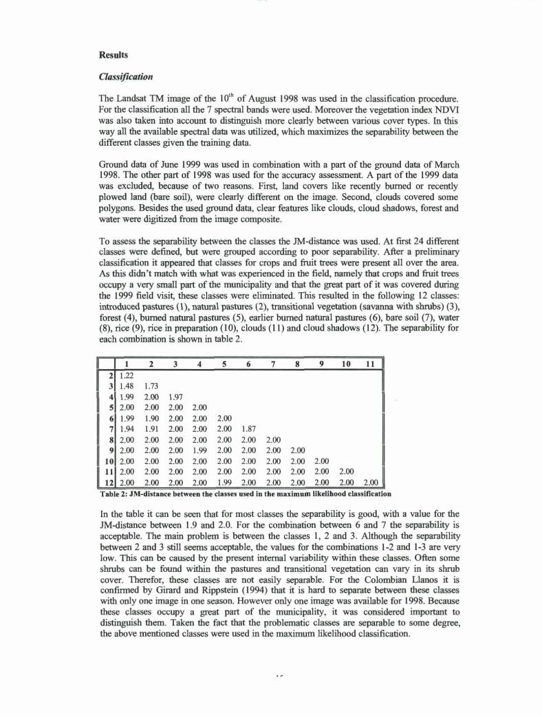
To assess the separability between the classes the JM-distance was used. At tirst 24 different classes were detined, but were grouped according to poor separability. After a preliminary classification it appeared that classes for crops and fruit trees were present all over the area. As this didn't match witb what was experienced in the tield, namely that crops and fruit trees occupy a very small part of the municipality and that the great part of it was covered during the 1999 tield visit, these classes were eliminated. This resulted in the following 12 classes: introduced pastures (l), natural pastures (2), transitional vegetation (savanna with shrubs) (3), forest (4), bumed natural pastures (5), earlier bumed natural pastures (6), bare soil (7), water (8), rice (9), rice in preparation (10), clouds (11) and cloud shadows (12). The separability for each combination is shown in table 2.

1

1 2 3 4 5 6 7 8 9 10 11 2 1.22

3 1.48 1.73 4 1.99 2 .00 l.97 ~ 5 2.00 2.00 2.00 2.00

6 1.99 1.90 2.00 2.00 2.00

7 l.94 1.91 2.00 2.00 2.00 1.87 8 2.00 2.00 2.00 2.00 2.00 2.00 2.00

9 2.00 2.00 2.00 1.99 2.00 2.00 2.00 2.00

10 2.00 2.00 2.00 2.00 2.00 2.00 2.00 2.00 2.00

11 2.00 2.00 2.00 2.00 2.00 2.00 2.00 2.00 2.00 2.00

12 2.00 2.00 2.00 2.00 1.99 2.00 2.00 2.00 2.00 2.00 2.00

Table 2: JM-dlstance between tbe classes used in tbe maxlmum likelihood classlficatlon

In the table it can be seen that for most classes the separability is good, with a value for tbe JM-distance between 1.9 and 2.0. For the combination between 6 and 7 the separability is acceptable. The main problem is between the classes 1, 2 and 3. Althougb the separability between 2 and 3 still seems acceptable, the values for the combinations 1-2 and 1-3 are very 1ow. This can be caused by the present intemal variability within tbese classes. Often sorne shrubs can be found within the pastures and transitional vegetation can vary in its shrub cover. Therefor, these classes are not easily separable. For tbe Colombian Uanos it is contirmed by Girard and Rippstein (1994) tbat it is hard to separate between these c1asses with only one image in one season. However only one image was available for 1998. Because tbese classes occupy a great part of the municipality, it was considered important to distinguish them. Taken the fact that the prob1ematic classes are separable to sorne degree, the above mentioned classes were used in the maximum likelihood classitication.

The maximum likelihood classification used the 12 classes with a threshold of 3.00 standard deviations. The result of this classification can be seen in annex 5. The accuracy of this classification has been assessed using available ground data collected in March 1998 and sorne additional digitized data. This resulted in the following confusion matrix.

3 6 1 7 8 9 10 12 o o

2 53 o o o o 3 o ~1 ~1 ~1 ~ ~1 ~1 4 o S 113~ ~1 ~1 ~1 ~ ~1 ~1 6 7 ~1 26~1 216~1 ~1 ~ ~1 ~1 8

1 9

1 ~ o o

~ o o o o 1891 122~ o i 10 o o o o o o o o

11 o o o o o o o 2075

1

12 o o 4 o o o o o o (] o 161 1 Total 25200 4808 4632 5606 527 1193 268 2169 1900 123S 2086 162

producer's accuracy (%) 83.9 67.2 83.0 96.6 992 95.5 100.0 100.0 100.0 IOO.C 100.0 99.~

Table 3: Confusloo matrb: for the mulmum likellbood classlficatlon

For most classes the producer's accuracy was very good. However, this does not always mean that a classified pixel in the image will coincide with its proper land cover, because it could be classified wrongly in another class. As could be expected from the separability, the smallest accuracy appears in the classes 1 to 3, that occupy 65 % of the municipality within the classificati.on. The overall accuracy was calculated weighing the producer's accuracy to their respective percentages in the classification within the municipality. This was done because almost 50% ofthe March 1998 ground data was taken in introduced pastures, which would bias the normal procedure to calculate overall accuracy. The calculati.on resulted in an overall accuracy of 84 %.

Before arriving at the final land use map, more processing had to be done. Clouds are not desirable in a satellite image. They were taken into account in the c1assification to ensure that these areas would not be classified erroneous. The 1996 classification was used to fill these areas. After this operation a filter was applied to eliminate small areas, that most probably have been classified incorrectly. This filter merges image value polygons smaller than 9 pixels with a connectedness of 4 (adjacent if pixels are in contact horizontally or verti.cally) with the largest neighboring polygon.

By examining the classification with a composite of the image, it was concluded that sorne parts ofthe image were clearly classified wrongly, because ofthe presence of opaque clouds. The composite could show rather well the proper land use in these areas. Therefor, 1.3% of the image was digitized according to the apparent land use and overlaid on the classification. Furthermore sorne tree plantations (fruit trees and rubber) were considered significant in the area and their coordinates had been taken in the field. These data were also overlaid on the classification. These adaptations resulted in the following land use map.