Errata for

A Guide to Microsoft Excel 2013 for Scientists and Engineers

by Bernard Liengme

Page 28 in part (b) the formula for F6 is =B5*B6^(1-F5)^0.2857, replacing B9 in the book with F5. This

yields 46.85185; the correct value is obtained in parts (d) and (e). In part (d) replace the two references

to (1 – B9) with (1 – F5).

Page 46 in the first sidebar CTRL+ALT should read CTRL+A.

Page 54, part (a): the first sentence needs an additional phrase: On Sheet2 of Chap4.xlsx, type in the text

shown in A1:C1 and in column E; note that the entry in E10 is in preparation for Exercise 3.

Page 76 part (a): should read “enter the values in A1:B5”.

Page 78 part (b): to be grammatically correct this should begin “Name C2 and C3 as…”. Page 78 part (d): the formula given for E6 has the incorrect comparison operator comparing B6 and qmax; it read =--AND(A6>=pmin, B6<=qmax). Note that an alternative formula for E6 would be =C6*D6. Page 78 part (e): should end with “…between the two words, and C16:E16 have been formatted to display percentage values.”.

Page 78 second paragraph under THE IF FUNCTION: in the formula at the end of the paragraph there is a misplaced comma; it should read =IF(A1, “Not Zero”, “Zero”) Page 79 second paragraph in NESTED IFS: in the formula the second comma in the formula is misplaced, it should read =IF(A1>10, “A1>10”,“A1 not >10”). Page 79 item (i) at bottom of page: the formula has an unnecessary comma after “Big”; it should read =IF(A1>50, “Big”,“Medium”).

Page 80, part (ii) under diagram: the formula has an unnecessary comma after “Big” and after “Negative”; it should read =IF(A1>10, IF(A1>50, “Big”,“Medium”), IF(A1<0, “Negative”,“Small”)).

Page 85 last line: the syntax for HLOOKUP is HLOOKUP(lookup_value, table_array, row_index_num,

range_lookup). Note the incorrect column_index_num is replaced by row_index_num.

NOTE: in all syntax listings bold tells the user that the argument is required while non-bold shows it is

optional.

Page 87 part (b): the reference to C4 should be to C3.

Page 87 part (c): should read “we could omit the fourth argument…”.

Page 87 part (d): should refer to C6’s fill handle.

Page 87 part (e): it is C8 that displays #N/A.

Page 88 part (a): the correct name for the workbook is Chap5.xlsx.

Page 92 in part (b) the second equation should read i i

iN 15 with the digit 1 in the second

summation rather than the letter i.

Page 94 the second equation in the introduction to Exercise 10 should read

i

i

i

ii

n

nxx

std1

)( 2

2 with

the term std shown as squared. Since this computes the square of the standard deviation, in the

worksheet we use SQRT to get just std.

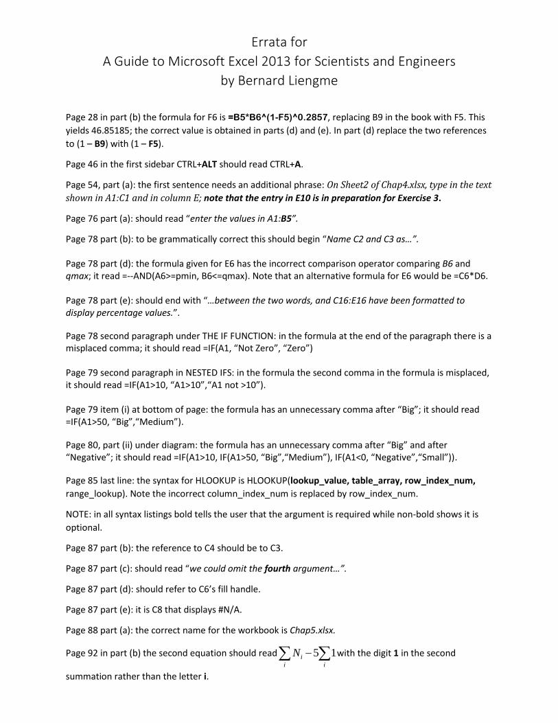
Page 105 Exercise 2: rows 1 through 9 are missing in Figure 6.2. The correct diagram for this Exercise is

shown below.

Figure 6.2

Page 105 Exercise 2 part (a) should read: enter the text shown in cells E1:I23 of Figure 6.2.

Page 169, the last sentence in the first paragraph needs a typo correction and perhaps a better

explanation: Note the primary vertical axis has been formatted with ‘display units’ set to 10,000 for

the N values.

Page 169 gives incorrect information for the formulas used in A13:B13, the actual formulas in the

worksheet are =LOGEST(B4:F4,B3:F3) with no LN function.

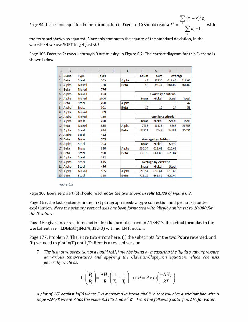
Page 177, Problem 7. There are two errors here: (i) the subscripts for the two Ps are reversed, and

(ii) we need to plot ln(P) not 1/P. Here is a revised version

7. The heat of vaporization of a liquid (ΔHv) may be found by measuring the liquid’s vapor pressure at various temperatures and applying the Clausius-Clapeyron equation, which chemists generally write as:

1

2 2 1

1 1ln or expv vH HP

P AP R T T RT

A plot of 1/T against ln(P) where T is measured in kelvin and P in torr will give a straight line with a slope –ΔHv/R where R has the value 8.3145 J mole-1 K-1. From the following data find ΔHv for water.

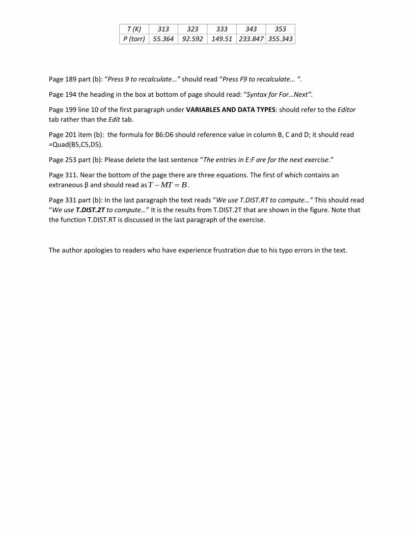
T (K) 313 323 333 343 353

P (torr) 55.364 92.592 149.51 233.847 355.343

Page 189 part (b): “Press 9 to recalculate…” should read “Press F9 to recalculate… “.

Page 194 the heading in the box at bottom of page should read: “Syntax for For…Next”.

Page 199 line 10 of the first paragraph under VARIABLES AND DATA TYPES: should refer to the Editor

tab rather than the Edit tab.

Page 201 item (b): the formula for B6:D6 should reference value in column B, C and D; it should read

=Quad(B5,C5,D5).

Page 253 part (b): Please delete the last sentence “The entries in E:F are for the next exercise.”

Page 311. Near the bottom of the page there are three equations. The first of which contains an

extraneous β and should read asT MT B .

Page 331 part (b): In the last paragraph the text reads “We use T.DIST.RT to compute…” This should read

“We use T.DIST.2T to compute…” It is the results from T.DIST.2T that are shown in the figure. Note that

the function T.DIST.RT is discussed in the last paragraph of the exercise.

The author apologies to readers who have experience frustration due to his typo errors in the text.