Error Analysis, Statistics, Graphing and Excel

Necessary skills for Chem V01BL

Error Analysis

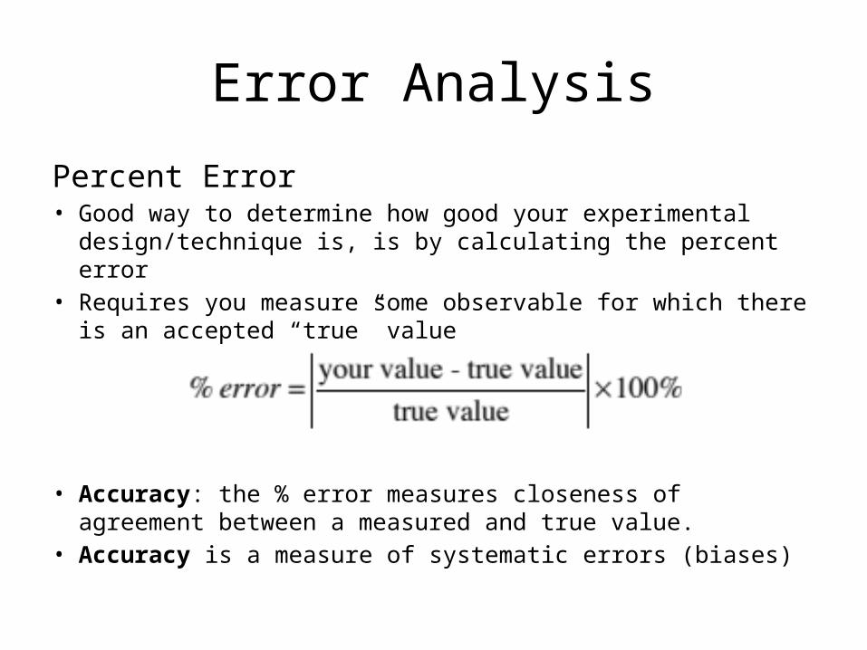
Percent Error• Good way to determine how good your experimental

design/technique is, is by calculating the percent error• Requires you measure some observable for which there is an

accepted “true” value

• Accuracy: the % error measures closeness of agreement between a measured and true value.

• Accuracy is a measure of systematic errors (biases)

Error Analysis

Mean Value• In experiments random errors exist. When measuring some

observable to assess these random errors we repeat measurements in independent trials

• We report the mean value

• We generally then report the % error for the mean value

Error AnalysisStandard Deviation• It is important to measure how large the random errors are in

an experiment• We measure this using the standard deviation σ• This normally requires at least 6 independent trials

• Can be evaluated for a column of data in Excel with the =STDEV(A1:A10) type syntax

• σ is a measure of precision. The smaller σ is, the more precise the measurement was.

Error Analysis

Standard Deviation Continued

• In particle physics they use the standard of 5σ for the declaration of a discovery

• At this level there is only a chance of 1 in 2,000,000 that the value was arrived at was a random fluctuation about the true value

Error Analysis

Standard Deviation Continued

Error Analysis

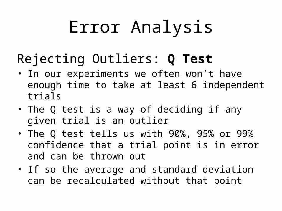
Rejecting Outliers: Q Test• In our experiments we often won’t have enough time to take

at least 6 independent trials• The Q test is a way of deciding if any given trial is an outlier• The Q test tells us with 90%, 95% or 99% confidence that a

trial point is in error and can be thrown out• If so the average and standard deviation can be recalculated

without that point

Error Analysis

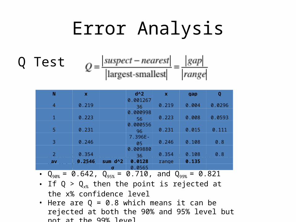
Q Test

If Q > Qx% then the point is rejected at the x% confidence level

N: 3 4 5 67 8 9 10

Q90%: 0.941 0.765 0.642 0.560 0.507 0.468 0.437 0.412Q95%: 0.970 0.829 0.710 0.625 0.568 0.526 0.493 0.466Q99%: 0.994 0.926 0.821 0.740 0.680 0.634 0.598 0.568

Error Analysis

Q Test

• With the data as it stands the average is 0.255±0.057• Q90% = 0.642, Q95% = 0.710, and Q99% = 0.821• If Q > Qx% then the point is rejected at the x% confidence level• Here are Q = 0.8 which means it can be rejected at both the

90% and 95% level but not at the 99% level• If we reject it the average becomes 0.230±0.031

N x d^2 x gap Q4 0.219 0.00126736 0.219 0.004 0.02961 0.223 0.00099856 0.223 0.008 0.05935 0.231 0.00055696 0.231 0.015 0.1113 0.246 7.396E-05 0.246 0.108 0.82 0.354 0.00988036 0.354 0.108 0.8av 0.2546 sum d^2 0.0128 range 0.135

σ 0.0565

Graphing and Excel• Graphing is a widely used technique for determining mathematical relationships

(correlations) between a dependent and independent variable• To determine if two variables are correlated can be measured by calculating the

coefficient of determination R2

• Here y(xi) is the value of the independent value for the dependent value and f(x i) is the function attempting model y=f(xi)

• As we shall see if R2>0.99 data fits the model

• We will routinely use Excel to plot two variables which are linearly correlated and use Excel to determine the equation for the line

• The slope of that line, and the intercept will both correspond to scientific observables that are of considerable value to us

Graphing and ExcelCorrelated data: ideal gas law• Find the relationship between the volume of 1 mole of O2 and its

temperature at 1 atmosphere

• The equation for the straight line where y = V and x = T gives

• The R2=1 means there is a perfect linear correlation between T and V

V(L) T(oC)

25 31.49

30 92.38

35 153.28

40 214.18

45 275.08

50 335.97 0 50 100 150 200 250 300 350 4000

10

20

30

40

50

60

f(x) = 0.0821056581804974 x + 22.4147274224972R² = 0.999999999119499

V vs T for 1 mole of O2 at 1 atm

T(Celcius)

V(L)

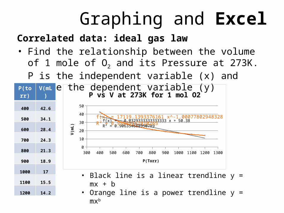
Graphing and ExcelCorrelated data: ideal gas law• Find the relationship between the volume of 1 mole of O2 and

its Pressure at 273K. P is the independent variable (x) and Volume the dependent variable (y)

P(torr) V(mL)

400 42.6

500 34.1

600 28.4

700 24.3

800 21.3

900 18.9

1000 17

1100 15.5

1200 14.2

300 400 500 600 700 800 900 1000 1100 1200 130005

1015202530354045

f(x) = − 0.0329333333333333 x + 50.38R² = 0.906354688950789

f(x) = 17119.1393376161 x^-1.00077802948328R² = 0.99999157010265

P vs V at 273K for 1 mol O2

P(Torr)

V(m

L)

• Black line is a linear trendline y = mx + b• Orange line is a power trendline y = mxb

Graphing and ExcelCorrelated data: ideal gas law• Find the relationship between the volume of 1 mole of O2 and its Pressure

at 273K. P is the independent variable (x) and Volume the dependent variable (y)

• When we plot P vs 1/V R2 = 0.99999, when we plot P vs V R2 = 0.90635. So

P(torr) 1/V(mL)

400 0.023474178

500 0.029325513

600 0.035211268

700 0.041152263

800 0.046948357

900 0.052910053

1000 0.058823529

1100 0.064516129

1200 0.070422535

300400

500600

700800

9001000

11001200

13000

0.010.020.030.040.050.060.070.08

f(x) = 0.0151830740641521 exp( 0.00133958121104467 x )R² = 0.975999062186756f(x) = 5.87245979808679E-05 x − 3.69772322639239E-06R² = 0.999986982411845

P vs 1/V for 1 mole of O2 at 273K

Series1Exponential (Series1)Linear (Series1)

P(Torr)

1/V

(mL-

1)

Graphing and ExcelUncorrelated dataHouse value versus Street Address

Graphing and Excel• Often data from a trendline fit is used to obtain certain observables.• With any experimentally measured quantity we need to estimate the

random error• In kinetics

0.0028 0.003 0.0032 0.0034 0.0036 0.00380

1

2

3

4

5

6

7

8

f(x) = − 5627.81307133434 x + 22.7299763301246R² = 0.921121461489257

ln(k) vs 1/T for the reaction of BrO3- with I- in the presence of an acid

Series1Linear (Series1)

1/T (K-1)

ln(k

)

• σEa and σln(A) are needed!

• can be calculated with LINEST function in Excel

Summary using LINEST

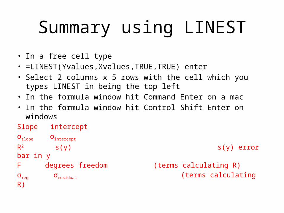
• In a free cell type• =LINEST(Yvalues,Xvalues,TRUE,TRUE) enter• Select 2 columns x 5 rows with the cell which you types

LINEST in being the top left• In the formula window hit Command Enter on a mac• In the formula window hit Control Shift Enter on windowsSlope interceptσslope σintercept

R2 s(y) s(y) error bar in yF degrees freedom (terms calculating R)σreg σresidual (terms calculating R)

Tonight

• Answer the problem set on pages 10-13• Each student must individually make a graphs of V vs T , V vs P,

1/V vs P. Each graph curve should be fitted using a linear trendline where the equation and R2 value is shown.

• Use the graphing procedure given on page 9• For question 4 calculate the standard deviations for the slope

and the intercept and attempt to put error bars using dy