Support for this research was provided in part by National Science Foundation grant numberSES91-22355. The second author acknowledges research grant support from the University ofSaskatchewan.

Error Bands for Impulse ResponsesChristopher A. Sims

Yale University

and

Tao Zha

Federal Reserve Bank of Atlanta

July 1995

We examine the theory and behavior in practice ofBayesian and bootstrap methods for generating errorbands on impulse responses in dynamic linear models. TheBayesian intervals have a firmer theoretical foundation insmall samples, are easier to compute, and are about asgood in small samples by classical criteria as are the bestbootstrap intervals. Bootstrap intervals based directly onthe simulated small-sample distribution of an estimator,without bias correction, perform very badly. We showthat a method that has been used to extend to theoveridentified case standard algorithms for Bayesianintervals in reduced form models is incorrect, and we showhow to obtain correct Bayesian intervals for this case.

1

1. Introduction

In interpreting dynamic multivariate linear models, impulse response functions are of centralinterest. Presenting measures of the statistical reliability of estimated impulse responses is there-fore important. On the other hand, such models have three features that raise difficulties forconstruction of classical confidence intervals:

i) Estimates of the underlying autoregressive reduced form parameters of such models havesampling distributions that depend strongly in shape as well as location on the true value of theparameters, especially in the neighborhood of parameters that imply non-stationarity;

ii) Impulse responses are highly nonlinear functions of the underlying autoregressive reducedform parameters; and

iii) The distribution of the estimate of a particular response at a particular horizon dependsstrongly on the true values of other impulse responses at other time horizons, with no apparentgood pivotal quantity available to dampen such dependence on nuisance parameters.

Most applied researchers are familiar with forming and interpreting confidence intervals insituations without these features, particularly in standard cases of estimators with asymptoticnormal distributions and an asymptotic “pivot”. More precisely, these standard cases are those inwhich we have an estimator $ ( )θ X based on data X for a parameter θ and an estimator $ ( )σ X for

the variability of $ ( )θ X such that $ ( ) $ ( )θ θ σX X−e j (the pivot) is asymptotically N(0,1). Confi-

dence intervals based on such an asymptotic approximation are convenient because they aresymmetric and can be formed using standard tables of the normal or t distribution. More impor-tantly, under mild regularity conditions their Bayesian posterior probability is asymptotically wellapproximated by their confidence level, regardless of the Bayesian prior. Because these cases areso common, applied work seldom carefully articulates the difference between confidence levelsand posterior probabilities. Decision makers without statistical training probably usually regard aneconometrician’s statement that “with confidence level 90%, θ is between a and b” as meaningthat, having observed the data, the econometrician regards .90 as a reasonable value to give, fordecision-making purposes, to the probability that θ lies in (a,b). But this is the Bayesian interpre-tation of the interval, not the classical one.

An exact 90% confidence interval does “contain the true parameter value with probability.90”, but this probability statement is only appropriate before data is observed. That is, before wesee X, it is reasonable to say that the probability that the confidence interval contains θ is .90.This does not mean in general that it is still reasonable after we see X to say that the probabilitythat the confidence interval contains θ is .90. The fundamental difference between a Bayesianapproach to inference and a classical approach is that the latter restricts itself to probabilitystatements based on pre-observation probability distributions, while the former aims at aiding theformation of reasonable probability statements about the parameter conditional on the observeddata.

2

Example 1

To remind oneself of why confidence levels are not decision-making probabilities given thedata, consider a case where we know that µ lies in (0,1) and observe two i.i.d. N(µ, σ) randomvariables X1 and X2 . It would be natural (though arguably not optimal) to form confidenceintervals from the pivot $ $µ µ σ−b g , where the “hats” refer to the standard sample mean and

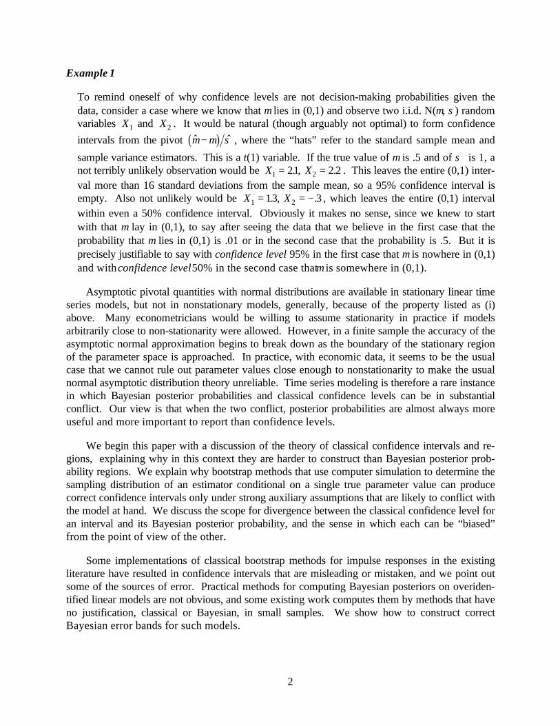
sample variance estimators. This is a t(1) variable. If the true value of µ is .5 and of σ is 1, anot terribly unlikely observation would be X X1 221 2 2= =. ., . This leaves the entire (0,1) inter-val more than 16 standard deviations from the sample mean, so a 95% confidence interval isempty. Also not unlikely would be X X1 213 3= = −. ., , which leaves the entire (0,1) intervalwithin even a 50% confidence interval. Obviously it makes no sense, since we knew to startwith that µ lay in (0,1), to say after seeing the data that we believe in the first case that theprobability that µ lies in (0,1) is .01 or in the second case that the probability is .5. But it isprecisely justifiable to say with confidence level 95% in the first case that µ is nowhere in (0,1)and with confidence level 50% in the second case that µ is somewhere in (0,1).

Asymptotic pivotal quantities with normal distributions are available in stationary linear timeseries models, but not in nonstationary models, generally, because of the property listed as (i)above. Many econometricians would be willing to assume stationarity in practice if modelsarbitrarily close to non-stationarity were allowed. However, in a finite sample the accuracy of theasymptotic normal approximation begins to break down as the boundary of the stationary regionof the parameter space is approached. In practice, with economic data, it seems to be the usualcase that we cannot rule out parameter values close enough to nonstationarity to make the usualnormal asymptotic distribution theory unreliable. Time series modeling is therefore a rare instancein which Bayesian posterior probabilities and classical confidence levels can be in substantialconflict. Our view is that when the two conflict, posterior probabilities are almost always moreuseful and more important to report than confidence levels.

We begin this paper with a discussion of the theory of classical confidence intervals and re-gions, explaining why in this context they are harder to construct than Bayesian posterior prob-ability regions. We explain why bootstrap methods that use computer simulation to determine thesampling distribution of an estimator conditional on a single true parameter value can producecorrect confidence intervals only under strong auxiliary assumptions that are likely to conflict withthe model at hand. We discuss the scope for divergence between the classical confidence level foran interval and its Bayesian posterior probability, and the sense in which each can be “biased”from the point of view of the other.

Some implementations of classical bootstrap methods for impulse responses in the existingliterature have resulted in confidence intervals that are misleading or mistaken, and we point outsome of the sources of error. Practical methods for computing Bayesian posteriors on overiden-tified linear models are not obvious, and some existing work computes them by methods that haveno justification, classical or Bayesian, in small samples. We show how to construct correctBayesian error bands for such models.

3

We undertake a number of computational exercises. We show that bias-corrections tobootstrap methods that have been suggested, but not yet widely used, in the literature are capableof producing classical confidence intervals whose coverage probability is in most, but not all, ofthe models we consider less divergent from their nominal coverage probabilities. Similar resultshave been obtained recently by Killian [1995], though that paper differs from our work in rulingout nonstationary parameter values. We show that Bayesian intervals, which are less difficult tocompute than the bootstrap ones, are competitive with the corrected classical ones even onclassical criteria. And we document the bias and imprecision in “corrected” classical bootstrapintervals as summaries of the implications of the data for the unknown true impulse responses (i.e.as summaries of the likelihood shape).

The paper’s objective is not mainly to advance the state of the art of constructing error bandswith good classical coverage probabilities.1 We regard classical coverage probabilities as ofsecondary interest and leave to others the daunting task of finding random intervals with bettercoverage probabilities in dynamic models. We document the fairly good performance of Bayesianintervals by classical criteria partly as a way to reassure classically trained econometricians thatBayesian intervals do not misbehave badly by the criteria they usually study. We examine theperformance by Bayesian criteria of “bias-corrected bootstrap intervals” motivated by classicalreasoning because these methods may be used in practice, and econometricians who share with usthe view that the Bayesian performance criteria are primary will want to know how deficient suchbootstrap methods are. Conscientious classical econometricians will be interested in these resultsalso, because they will recognize that confidence levels are not decision-making probabilities andwill want to warn readers or clients of cases where the discrepancy is likely to be large. Our mainobjective is to show that Bayesian intervals are relatively straightforward to compute and well-behaved and to show how to construct them for overidentified models, where there are some non-trivial computational difficulties.

2. Confidence Interval Fundamentals

Suppose we have a parameter space Θ whose elements θ index probability distributions forobservable data X that lies in the sample space Ω. Classical confidence levels and Bayesianposterior probabilities are both ways of associating probabilities with subsets of Θ. Bayesianspostulate a joint probability distribution over Θ Ω× and associate with S ⊂ Θ , after observingdata X, its posterior probability P S X . Classical inference avoids putting probability

distributions on Θ. It insists that S be regarded as varying randomly with X. IfP S Xθ θ α∈ = −( ) ( )1 for all θ, S ⋅b g is said to be a (1-α)% confidence region for θ. Sometimes

the definition is weakened to requiring only that P S Xθ θ α∈ ≥ −( ) ( )1 . With the inequality, we

1 We try to follow recent suggestions in the literature for improving performance ofbootstrapped error bands in dynamic models, and our computations include consideration of somemodels larger than those previously analyzed in Monte Carlo studies of such bands.

4

will refer to the interval as a conservative (1-α)% confidence interval, while with the equality wewill refer to it as an exact (1-α)% confidence interval.

A (1-α)% confidence region is equivalent to a collection of hypothesis tests with significancelevel α:2 Given S X( ) , form a test of H0 0:θ θ= for each θ 0 ∈Θ by rejecting when θ 0 ∉S X( ) .Given a set of tests with significance level α for H0 0:θ θ= , one for each θ 0 ∈Θ , and with rejec-tion regions R( )θ 0 , form S X( ) as θ θX R∉ ( )m r .

Confidence levels and posterior probabilities are related. Suppose S ⋅b g is a ( )%1− α confi-

dence region and consider the subset of Θ Ω× defined as V X S X= ∈θ θ, ( )m r . Denoting the

Bayesian marginal distribution on Θ (usually called the prior) by π, we can write

P V P V d P S X d= = ∈z zθ π θ θ θ π θ( ) ( ) ( )Θ Θ

. (1)

From (1) it is clear that P V = −1 α if S ⋅b g is exact and P V ≥ −1 α if S ⋅b g is conservative.But we can also write

P V P V X dX P S X X dX= = ∈z zµ θ µ( ) ( )Ω Ω

b g , (2)

where µ is the marginal distribution over Ω. Equations (1) and (2) together imply that an exactconfidence level is the mean over X of Bayesian posterior probabilities. Thus Bayesian posteriorprobabilities for S(X) cannot differ from the classical confidence level in the same direction for allX. Any tendency for posterior probabilities to be smaller than the confidence level for some Xmust be balanced by their being larger for other X. Also, if a conservative confidence level isclose to one, Bayesian posterior probabilities for S(X) must be as high as the confidence level withhigh probability. (These results depend on the assumption of a proper prior probability on Θ andmay not carry over to Bayesian posterior probabilities generated from improper prior p.d.f.’s thatdo not have a finite integral.)

Bayesian posterior probabilities depend in general on the prior distribution π over Θ. Since πmust come from a source other than the data at hand, econometricians and statisticians rightlyresist making their analysis dependent on such an arbitrary and possibly subjective element.Bayesians reporting data analyses for wide audiences, though, do not make their analysis depend-ent on a subjectively chosen π (see Hildreth [1963] for an explicit discussion). Instead they try tosummarize the form of the likelihood in a way that may be useful to a wide class of readers whomay have differing priors and loss functions. This may involve treating the normalized likelihooditself as a p.d.f. on Θ (i.e., using a “flat prior”), or it may involve using some transparent andstandard “reference prior” that will allow readers to adjust conclusions to reflect their own prior

2 A significance level can be conservative or exact, just as with a confidence level.

5

beliefs. In this paper we concentrate on Bayesian analysis with flat priors.3 Besides their useful-ness as a transparent reporting device, flat priors can also be justified by the fact that in largesamples posterior distributions under flat priors will generally approximately match those underany prior that has non-zero, continuous density in the neighborhood of the true parameter value.

To verify that S(X) has a confidence level ( )%1− α we need to know how it is distributed foreach θ in Θ. The idea of the bootstrap is to approximate the distribution of X at the true value ofθ by the distribution of X at some estimated point $θ in Θ. It may seem that, because thebootstrap generates an accurate estimates of the shape of the finite-sample distribution of $θ atone point in the parameter space, that it is generating exact small-sample confidence intervals. Infact, though, this method produces exact small-sample confidence intervals only under strongassumptions, rarely met in practice, about the nature of the dependence of the distribution of X onθ, as the following two examples illustrate.

Example 2

Suppose the p.d.f. of a scalar X is

f XX

X( ; )

exp logµ

µ

µ π=

− − +

− +

12

2 1

1 2

b gd ib g

on the half-line where X > −µ 1. That is, X − +µ 1 is lognormal with log X − +µ 1b gdistributed as N(0,1). The p.d.f. is plotted in Figure 1 for two different values of µ. If weobserve X=1, the likelihood has the same shape as the p.d.f. for X, but with the reverseorientation, as shown in Figure 2. A Bayesian posterior under a flat prior would produce a“highest posterior density” region with probability .95 as −197 19925. , . . This interval leavesmuch more probability in the left than in the right tail. An equal-tailed interval is −2 72 186. , . .Because this problem is one with the parameter affecting the distribution of X purely through alocation shift, Bayesian posterior probabilities and confidence levels coincide exactly. The factthat the intervals spread out over the area below X+1 while the distribution of X spreads outover the area above µ-1 makes perfect sense. After all, X cannot be below µ-1, so having seenX we know that µ cannot be above X+1.

In constructing the intervals discussed in example 2, we used knowledge of the entire struc-ture of the dependence of the distribution of X on µ. What if instead we had used computersimulation to find the distribution of X with µ set equal to 1, the observed value of X? This iswhat the “parametric bootstrap” would do. What Hall [1992] (and we, henceforth) call the equal-tail “percentile interval” is then constructed as follows. Let F X( ; )µ denote the c.d.f. of X when

3 In simple linear models posterior probabilities and confidence levels coincide under certainforms of flat prior. This is not true in general, however, and is very far from true in dynamicmodels near the boundary of the stationary region.

6

µ is the true value of the parameter. We suppose that simulation gives a perfectly accurateestimate of F X( ; )1 . We form our interval for µ by finding a and b such that F a( ; ) .1 1 025− = ,F b( ; ) .1 1 975+ = . Then the interval is [1-b, 1+a]. But this bootstrap interval coincides with theflat-prior Bayesian equal-tailed .95 probability interval. We seem to have arrived at an intervalthat should satisfy everyone, Bayesian or classical, on the basis of calculating only F( , )⋅ 1 , withouthaving to know the distribution of X for any other value of µ.

The bootstrap percentile interval of example 2 can be contrasted with the other-percentileinterval, which would be [1-a, 1+b] in example 2. It is obviously a terrible choice in example 2, asit includes µ ' s greater than 2, while it is in fact impossible for µ to be above 2. But as we nowsee in example 3, it is possible that F( , )⋅ 1 is exactly what was computed in example 2, and for theother-percentile interval to have correct coverage probability and to coincide with a Bayesianinterval with posterior probability matching the confidence level.

Example 3

Suppose that log( )X is distributed N(log(µ),1). When µ = 1, this gives X the same distribu-tion as for Example 2 when µ = 1 there. However, as can be seen by comparing Figures 1 and3, the distribution of X changes as µ deviates from 1 in quite different ways in the twoexamples. Here Z X N= log( ) ~ ( , )ν 1 , where ν µ= log( ) . It seems natural to use the normallydistributed Z −ν as a pivot, then convert our confidence interval on ν into a confidenceinterval on µ. This produces as a 95% confidence interval on µ, [.141,7.10]. The equal-tailedflat prior Bayesian posterior 95% probability interval is not the same, but it is similarly skewed,at [.37,17.4]. The likelihood, as can be seen in Figure 4, is similar in shape to the p.d.f., butdamps more slowly as its argument increases. The flat-prior posterior probability of theclassical interval is about .83. If the prior is flat on log( )µ rather than on µ itself, though, sothat the prior density is 1 µ , the posterior equal-tailed 95% interval is identical to the classical95% equal-tail confidence interval.4

As these examples illustrate, the fact that the bootstrap gives us accurate information aboutthe small-sample distribution of an estimator or statistic at a particular point in the sample spacedoes not in itself suggest that it is giving us small-sample accuracy in confidence intervals.Asymptotic distribution theory does tell us that under broad regularity conditions many estimators$θ have distributions in large samples that are close to normal and depend on the true parameter θapproximately via a pure location shift. This situation gives asymptotic justification to bootstrapconfidence intervals, but not in general to any asymmetries they may show. With strongerregularity conditions, it is possible to show that bootstrap intervals of certain types, or with

4 The flat prior on log( )µ is the Jeffreys prior for this example. A prime motivation for theJeffreys prior is to achieve invariance of a standardized “flat” prior to parameter transformations,so it is natural that it should lead us to the same conclusion as would transforming the probleminto Z,ν space. In Example 2 the Jeffreys prior is an ordinary flat prior.

7

certain corrections5, are asymptotically second-order accurate in a certain sense. Howeversecond-order accurate intervals often misbehave in finite samples, and in any case the regularityconditions they invoke appear to be violated in the neighborhood of unit roots for dynamicmodels.

3. Dimensionality

In this paper we are concerned primarily with confidence intervals on dynamic models’impulse response functions. The point that an exact 1− αb g% confidence set S Xb g is equivalentto a collection of tests of point null hypotheses, all with exact significance level α, suggests ageneral approach to finding confidence regions in a multi-dimensional parameter space, but it doesnot provide help in finding confidence intervals for individual elements of the parameter vector. Ifthe parameter space is Rk and we want a confidence interval on θ1 , the first element of the

parameter vector, then we are looking for a confidence region in Θ of the form S X Rk1

1b g× − .Confidence regions assembled from a collection of point hypothesis tests will not take this formunless the hypothesis tests are all based on statistics whose distributions do not depend on θexcept through θ1 . Though in the leading special case of the Gaussian linear regression modelsuch statistics (the usual t-statistics on individual coefficients) exist, they are not in general easy tofind. Of course it is possible to find a conservative confidence level for an arbitrary random setS Xb g (since it is just max

θθP S Xb g ), but if P S Xb gθ varies a great deal with θ, conservative

confidence levels may be misleading.

A Bayesian approach has no more difficulty with evaluating the posterior probability of aregion with the form S X Rk

11b g× − than with a region of any other form.

More generally we may be interested in a subvector of θ, with the remainder of θ regardedas nuisance parameters. For a Bayesian approach, this simply requires integrating over thenuisance parameters in forming probability statements, a straightforward, if possibly difficult, task.For a classical approach, the difficulties are more fundamental, because all probability statementsmust condition on the full parameter vector, whether they are “nuisances” or not.

When an analytic expression for the likelihood function is available, a Bayesian approach togenerating a posterior probability interval or region is much easier than bootstrap approaches togenerating confidence intervals or regions. With a given data set, the Bayesian problem is tocharacterize the shape of the posterior, which is a single distribution whose form is given by thelikelihood, or by the likelihood multiplied by the prior p.d.f. Sampling from this distribution maybe a non-trivial problem if the likelihood has a non-standard form, but there are well-understoodcomputational techniques for attacking it. But the existence of an analytic form for the p.d.f. doesnot save a classical approach from the need to analyze the form of many distributions -- the

5 What Hall [1992] calls the percentile-t interval and the BCA interval of Efron and Tibshirani[1993] are examples.

8

distributions of the data for each possible value of the parameter. Of course some parametervalues may be so far from fitting well that we can ignore them, and continuity may allow us toapproximate the behavior of P X θ over a continuum of possible values for θ from knowledge

of its behavior for a finite number of values of θ, but in multivariate models the required numberof values of θ is likely to be large.

4. Error Bands for Multivariate Dynamic Models

Consider a model of the form

y t g t y t y t k( ) ( ), ( ),..., ( )= − −ε β1c h (3)

with ε ( )t independent of y t s( )− , all s>0, and having p.d.f. h ⋅ Ωc h . If ε ( )t is of the same

dimension as y(t), and if we have an analytic expression for the jacobian dy t d t( ) ( )ε ,6 then (3)allows us to write a p.d.f. for y(1), ..., y(T) conditional on y(0), y(-1), ..., y(-k+1), β, and Ω ,which we will label

p y y T y y k( ),..., ( ) ( ),..., ( ), ,1 0 1− + β Ωc h . (4)

It is common but not universal practice to treat (4) as the likelihood function. It is actuallythe likelihood function only if the distribution of y y k( ),..., ( )0 1− + does not depend on unknownparameters, or depends only on unknown parameters unrelated to β and Ω. If (3) is consistentwith y being ergodic, then it is natural to take the ergodic marginal distribution ofy t y t k( ),..., ( )− , which of course in general depends on β and Ω, as the distribution fory y k( ),..., ( )0 1− + . This is then combined with (4) to produce a p.d.f. for the full vector ofobservations y k y k y T( ), ( ),... ( )− + − +1 2 . There are three reasons this is not often done: it oftenmakes computations much more difficult; it requires that we rule out, or treat as a separate specialcase, non-stationary (and thus non-ergodic) versions of the model; and it may not be plausible thatthe dynamic mechanism described in (3) has been in operation long enough, in unchanged form, togive y y k( ),..., ( )0 1− + the ergodic distribution. The last two points are related. A non-stationary model has no ergodic distribution. A near-non-stationary model may have an ergodicdistribution, yet it may imply that the time required to arrive at the ergodic distribution fromarbitrary initial conditions is so long that imposing the ergodic distribution on y y k( ),..., ( )0 1− +may be unreasonable.

6 If ε is of higher dimension than y, we in effect have a latent variable, and integration overpart of the ε vector is required to form the likelihood. If ε is of lower dimension than y, theimplied distribution for y is singular, which ordinarily makes the model conflict too sharply withthe data to be usable for inference.

9

Bayesian inference would ideally use the ergodic distribution for the initial conditions atparameter values well within the stationary region of the parameter space, then shift smoothlyover to a distribution less connected to β and Ω as the non-stationary region is approached. Sucha model is likely to be application-dependent, however, and in the remainder of this paper we treat(4) as the likelihood. We also hold initial conditions fixed in generating Monte Carlo samples ofy(1), ..., y(T) when we evaluate classical coverage probabilities.7

Models in the class we consider here, then, have an analytic likelihood function and thereforemake exact Bayesian posterior probability calculations much easier than exact classical confidencelevel calculations. In fact much of our analysis will focus on the case where g is linear in β and his Gaussian, which makes the log likelihood quadratic in β, i.e. Gaussian in shape, in small andlarge samples, for stationary and non-stationary models.

For a general model of the form (3), there is ambiguity about how “impulse responses” oughtto be defined. Here, though, we consider only models such that g is linear in ε ( )t , so that theresponse a sij ( ) of y t si ( )+ to ε j t( ) is easily and unambiguously defined. By applying (3)recursively, we can solve for y t s( )+ as a function of ε ε ε( ), ( ),..., ( )t s t s t+ + −1 andy t y t k( ),..., ( )− −1 . Then

a sy t s

tiji

j( )

( )( )

=+∂

∂ε(5)

depends only on β, not y or ε, and can be found by elementary matrix operations.8

We focus our attention entirely on confidence or probability intervals for individual responsesat particular horizons, i.e. for single a sij ( ) values. Usually our interest is actually in the shape ofthe function aij ( )⋅ , i.e. of the whole pattern of the response over time, or even in an interrelated

7 On this latter point we differ from Killian [1995]. Conditioning on initial data values informing the likelihood or in constructing estimators (on which point Killian’s practice matchesours) amounts to ignoring potential information in the initial observations. Conditioning on themin doing Monte Carlo simulations of the data-generation process amounts to recognizing thedistinction between initial conditions that generate more and less informative samples. If theinitial y’s show unusually large deviations from their steady-state values, the sample is likely togenerate unusually sharp information about the parameters. It does not make sense to calculatecoverage probabilities that average across informative and uninformative samples when it is easyto take account of the fact that we have been lucky (or unlucky) in the initial conditions of theparticular sample at hand.

8 Note that, though the impulse responses as defined here coincide with the coefficients of themoving average representation (MAR) for stationary, linearly regular models, they are alsodefined for nonstationary models where no MAR exists.

10

set of such patterns of response. Confidence intervals or probability bands are often displayed ingraphs showing an estimated aij ( )⋅ plotted as a function of time horizon s along with the upperand lower limits of confidence intervals or probability bands on the individual a sij ( ) values. Butposterior distributions on a sij ( ) values or sampling distributions of estimates of a sij ( ) values arelikely to be dependent across s, i, and j, and the nature of the dependence will differ acrossapplications or samples. This raises problems in reporting results similar to those arising inregression models, where the collection of confidence intervals on individual coefficients may notgive an accurate picture of the nature of uncertainty about the whole coefficient vector. We leaveto future research the problem of how to provide more thorough characterizations of uncertaintyabout the a’s.9

5. Bias-Correcting the Bootstrap

The usual parametric bootstrap procedure begins with an estimate $ ( )θ X based on the

observed sample X. It then generates the distribution function F X⋅ $ ( )θe j for $ ( )θ X ∗ , where X ∗

is a Monte Carlo random variable generated from the distribution X would have if $ ( )θ X were the

true value of θ. If it turns out that the distribution of $ ( )θ X ∗ is not centered at $ ( )θ X , this

suggests that the original estimate $ ( )θ X was biased as an estimate of θ. Does this mean we

should adjust $θ for bias before proceeding?

As should be clear from our examples 2 and 3 above, there is no prima facie case for bias-adjusting if the percentile interval is used in generating the bootstrap confidence interval. Thisinterval, because it is based on reflecting the bootstrap sampling distribution of $θ about thepseudo-true-value $ ( )θ X , automatically accounts for bias. Bias-adjustment does not in generalmake an estimator more accurate in the sense of lowered root mean squared error (RMSE), andindeed when applied as here to a maximum likelihood estimate it is more likely than not to worsenRMSE over some range of parameter values. But most applied work has used the other-percentile interval, which, as is clear from example 2 above, is badly affected by bias. The mainintuitive appeal of the other-percentile interval is its transformation invariance, and Efron and

9 Though we have some ideas. If the a’s were jointly Gaussian, one could treat thecoefficients in aij ( )⋅ as a jointly normal vector and display the largest few and smallest fewprinciple axes of their p.d.f. contour ellipsoids. When plotted, these would show which kinds ofvariation in aij ( )⋅ are ill-determined by the likelihood function and which kinds are more sharplydetermined. This idea might be helpful despite the fact that the posterior on the aij ( )⋅ ’s is notGaussian. We do not think it very helpful to construct bands such that the posterior probabilitythat responses are contained entirely within the band is 1-α, any more than it is useful to inflateconfidence intervals in a regression model until the rectangular region defined by their intersectionhas posterior probability 1-α.

11

Tibshirani [1993] discuss ways to adjust it for bias in such a way that it retains this property.Their adjustment works directly with the confidence interval and in effect adjusts for median bias,not expectational bias.

Many applied studies have used the RATS Monte Carlo procedure for constructing Bayesianerror bands for VAR impulse responses, usually with little or no discussion of underlyingmethodological issues. Blanchard and Quah [1989], Lastrapes and Selgin [1994], and Runkle[1987] use bootstrap methods, relying basically on other-percentile methods without bias-correction. Runkle uses it without modification; Blanchard and Quah modify it to avoid suchstrong bias that the interval fails to include the point estimate; and Lastrapes and Selgin followBlanchard and Quah in this latter respect. Koop [1992] computes Bayesian intervals for theBlanchard-Quah impulse responses, noting how different they are,10 and also provides analgorithm to handle models with differing lists of right-hand-side variables across equations. It ispossible simply to derive analytical expressions for asymptotic standard errors of impulse responseestimates and to use them, together with the normal asymptotic approximation, to arrive atconfidence intervals, as shown by Lutkepohl. [1990] and Mittnik and Zadrozny [1993], and thisapproach has been used in practice, e.g. by Poterba, Rotemberg and Summers [1986] and Runkle[1987]. Bands constructed this way are always symmetric about the estimates and shrink to zerowith the time horizon in stationary models. Bootstrap methods are motivated by a desire to avoidthese unrealistic properties of the asymptotic intervals. Killian [1995] finds in a Monte Carlostudy that the symmetric intervals arrived at this way have poor small-sample properties comparedto other alternatives.

Killian proposes to adjust the estimator $ ( )θ ⋅ itself for expectational bias. This is not at all thesame thing as what Efron and Tibshirani [1993] call bias adjustment,11 and we see no basis inexisting asymptotic distribution theory for thinking that this will work generally to produce betterconfidence intervals. It casts aside the transformation invariance of the other-percentile interval.Nonetheless, this form of bias adjustment seems to help. Killian reports trying other methods withfirmer foundations in asymptotic theory without good result, and we have ourselves found thatsome other approaches to generating bootstrap intervals do not perform systematically better, interms of coverage probability, than Killian’s intervals.12 Because our aim is to compare the

10 Though, as we will see below, most of the stark asymmetry found by Blanchard and Quaharose from an error in their calculations.

11 See Hall [1992], p.129 for some elaboration of the point that what is called “biascorrection” in the literature of bootstrapped confidence intervals is not correction of thebootstrapped estimator for bias.

12 In some cases we examined, the percentile method produced small deviations from itsnominal coverage probability more often than did the other-percentile method with Killian’scorrection, while it deviated by more than .20 much less often. In others (our version of) Killian’smethod produced strictly better results than the percentile method. We also tried applyingKillian’s type of bias-correction directly to the confidence intervals on impulse responses rather

12

Bayesian intervals we prefer with bootstrap alternatives actually in use, not to advance furtherinto the dense and (in our view) fruitless thickets of classical bootstrap theory, we use a variant ofKillian’s approach as representative of bootstrap methods.

Killian suggests bias correction by what he calls “bootstrap after bootstrap.” Its motivation isas follows. We begin by forming a point estimate $ ( )θ X and using it as a pseudo-true value in

generating an artificial sample of draws X ∗ from the distribution of X. Denoting the mean of theMonte Carlo sample of $ ( )θ X ∗ values by θ ∗ , we estimate the bias in $ ( )θ X as $ ( )θ θX − ∗ andarrive at a bias-corrected estimate

$$ ( ) $ ( ) $ ( ) $ ( )θ θ θ θ θ θX X X X= + − = −∗ ∗e j 2 . (6)

Killian’s basic idea is that $$ ( )θ X should be a better estimate than $ ( )θ X , so we will get better

confidence intervals if we bootstrap it rather than $ ( )θ X .

But to bootstrap $$ ( )θ X requires what Killian calls “bootstrap within bootstrap” calculations.

For each Monte Carlo draw X ∗ we have to draw a new Monte Carlo sample to find the biascorrection. The number of Monte Carlo draws is thus squared, which is likely to be infeasible.Killian points out that there is asymptotic justification for simply using the original biasadjustment, $ ( )θ θX − ∗ , for all the Monte Carlo draws rather than calculating a new adjustmentfor each draw. This means that the confidence interval is constructed in two steps -- an initialbootstrap calculation to find the bias correction, then an additional bootstrap calculation to findthe bias-corrected confidence interval. He calls this “bootstrap after bootstrap,” and it doublesthe number of Monte Carlo draws instead of squaring it.

Our procedures for computing coverage probabilities and bias corrections do differ fromKillian’s in certain respects. He follows Runkle [1987] in computing coverage probabilities basedon the unconditional distribution of the time series sample implied by the model’s stationaryergodic distribution. As we explained above, our view is that there is seldom good a priori reasonto exclude nonstationary models, and that in any case coverage probabilities using the distributionof the data conditional on the initial observations are more useful than unconditional coverageprobabilities.13 We therefore use the conditional distribution, given initial conditions, when wecompute coverage probabilities. Because Killian must restrict attention to stationary versions of

than to the autoregressive parameter estimates, confirming Killian’s experience that this did notwork as well.

13 Killian apparently follows Runkle [1987] in drawing initial conditions as randomsubsequences of the observed sample values. Whenever the model contains roots on the order of(T-2)/T (where T is sample size) or larger in absolute value, though, this procedure will give aseriously distorted picture of the true unconditional distribution of initial conditions.

13

models to make his procedures internally consistent, he uses ad hoc procedures to map parametervalues implying nonstationary models back into the stationary region of the parameter space whenhe is generating Monte Carlo draws. We include nonstationary draws of the parameter vectorwithout alteration. We believe this better reflects actual practice, since reports of estimates thatseem to imply slightly explosive behavior are not uncommon in the literature.

We follow Killian in using the semi-parametric bootstrap. That is, we draw with replacementfrom the sample distribution of residual vectors in generating artificial bootstrap samples. Thealternative would be to use the fully parametric bootstrap, drawing from the joint normaldistribution with covariance matrix equal to the sample estimate. When we evaluate coverageprobabilities, we of course draw from the hypothesized true model’s distribution, which involvesdrawing from the normal distribution for the residuals.

6. Some Simple Bivariate Cases

Bayesian and classical error bands for impulse responses may be similar or different. Whenthey differ, the classical interval may be misleading by Bayesian criteria or not so misleading, andvice versa. And classical intervals generated by bootstrap computations, which are rigorouslyjustified only asymptotically, may perform well or badly in finite samples by classical criteria. Allthese cases actually occur, and we begin by displaying some simple models that may give someinsight into the range of behaviors of error band calculations as the parameter values of the modelchange.

We will examine a model of the form

y t c Ay t t

t N

( ) ( ) ( )

( ) ~ ,

= + − +1

0

ε

ε Ωb g (7)

with ε ( )t independent of past y’s. First suppose

A =LNM

OQP

LNMOQP =

LNM

OQP

. .. .

.9 11 9

11

116 11 1

, c = , Ω . (8)

This model gives y a single unit root and a co-integrating vector [1 -1]. The stable root in thesystem is .8, and the constant term feeds in to the nonstationary part of the system to generate alinear trend component. Such a model is known to have asymptotic Gaussian distribution theoryfor the OLS estimates of A,14 so we might expect it to be easy to construct intervals with goodclassical coverage properties and expect classical coverage probabilities to be close to flat-priorBayesian posteriors. To a considerable extent, this is what we find.

14 Sims, Stock and Watson [1989], for example, show that since in this model each variable isa linear combination of a nonstationary variable dominated by linear trend and a stationaryvariable, the coefficients estimated will be jointly normal, asymptotically.

14

In all the results reported below for reduced-form models, the responses are triangularlyorthogonalized, with the first variable’s innovation producing an immediate response in thesecond variable, but not vice versa. This means that the first-period response of variable 1 tovariable 2 is always identically zero so that coverage probabilities are not meaningful. We reportzeros in these positions in tables as placeholders. All the calculations for these models involvedata sample sizes of 100, 1000 Monte Carlo draws in the construction of the Bayesian orbootstrap interval for each data set, and 600 Monte Carlo draws of data sets.

We deviate from the procedure suggested in the RATS manual (and from early drafts of thispaper) in using bands based on quantiles of simulated distributions rather than on second momentsof the simulated distributions. For some cases (the Y-M model below, for example) one-standarderror bands about means of Monte Carlo distributions are practically identical by eye to 68%quantile intervals. But for other cases, particularly at long horizons, the differences aresubstantial. Quantile-based intervals make more demands on computer storage, because theyrequire storing at least some fraction of draws for sorting, while moment-based intervals cansimply cumulate sums of products of simulated values, but our experience is that the quantile-based intervals are sometimes different and more informative.

The right-hand panel of Table 1 shows that Bayesian flat-prior .68 posterior probability15

regions for this model have essentially exactly .68 classical coverage probabilities, to withinMonte Carlo sampling error. Just one response, the t=2 response of y2 to y2 , is slightly outsidea band of two Monte-Carlo standard errors about .68. The left panel shows that the bootstrapintervals have modest, but definite, coverage errors, all at the short time horizons and all in thedirection of undercoverage. Table 2 shows that, for a random sample of four time series drawnfor this process, the bootstrap interval often, but not always, showed substantial error as ameasure of posterior probability. Between intervals with equal posterior probability or coverageprobability, the one that tends to be shorter is best, because it better concentrates attention onhigh-probability density regions. As we can see from Table 3, the Bayesian intervals for thismodel tend to be shorter on average, especially at longer horizons.

Having thus begun with a case where by every criterion, Bayesian or classical, Bayesianintervals are better, we now turn to a case in which the Bayesian intervals are bad by classicalcriteria. Here we use the parameter setting

15 Through most of this paper we concentrate on intervals with coverage or posteriorprobability .68 (one standard error in the Gaussian case). In much applied work .90, .95 or .99probability intervals are used. We think that as econometricians move away from the practice ofpretesting and data-mining to arrive at small models with inflated t-statistics, it would be a goodidea to make one-standard-error intervals the norm, as they are likely to be closer to the relevantrange of uncertainty. In examining “error” in intervals, use of high-probability intervalscamouflages the occurrence of large errors of over-coverage. A ridiculously large .95 intervalmay have coverage probability of only .995, wrong by “only” .045. Finally, accurate Monte-Carlocalculation of the end points of high-probability intervals generally requires considerably largernumbers of Monte Carlo draws.

15

A =LNM

OQP

LNMOQP =

LNM

OQP

1 00 1

11

1 00 1

, c = , Ω . (9)

This parameter setting produces two unit roots, thus no cointegration, and makes the twocomponents of y two independent random walks with the same drift. As can be seen from Table4, both Bayesian and bootstrap intervals deviate substantially from the nominal .68 coverageprobability at most time horizons, with the deviations uniformly in the direction of undercoverage.Furthermore, with the exception of a few low values of t, the undercoverage is worse for theBayesian intervals.

Of course this extreme undercoverage for the Bayesian intervals reflects the fact thatstationary models are likely to be estimated with larger sampling error than non-stationarymodels.16 Bayesian inference produces intervals that are biased according to pre-sampleprobabilities because such inference takes appropriate account of the asymmetries in samplingdistribution dispersion between stationary and non-stationary models.17 We might expect then,that classical intervals would do badly in this situation in the sense that their posterior probabilitieswould deviate substantially from their nominal confidence levels. Table 5 shows that this isindeed the case, with the bootstrap intervals tending to have probability exceeding .68 at longtime horizons and probability below .68 at some short horizons. We show only one representativerandom draw of a coefficient estimate for this case, because there is not much qualitative variationacross samples in the results. Though the deviation from .68 is sometimes a little less, sometimesquite a bit worse, the pattern of excessive probability at long time horizons and deficientprobability at some short horizons is pervasive. As can be seen from Table 6, the tendency ofBayesian intervals to have both lower coverage probability and lower posterior probability thanthe bootstrap intervals corresponds to a pronounced tendency for the Bayesian intervals to benarrower, particularly at long time horizons. Note the contrast with the cointegrated model,where the shorter length for the Bayesian intervals did not correspond to any general tendency forthem to have less probability, either pre- or post-sample.

Next we consider two examples of bivariate models based on economic time series. For boththese models we use 1000 Monte Carlo draws in generating Bayesian or bootstrap intervals for agiven data set, and 600 draws of data sets in constructing coverage probabilities.

16 See Sims and Uhlig [1991] for a more extended discussion of this point.

17 The performance of the Bayesian interval by classical criteria for this particular parametervalue could of course be improved by use of a prior favoring this parameter value. In fact wehave verified that, for example, a standard Litterman prior, with standard error .045 on own lagcoefficients and .022 on cross lag coefficients produces .68 posterior probability intervals whosecoverage probability is uniformly better than that of the bootstrap model for this parametersetting. Of course this improved classical performance at this point in the parameter space isprobably offset by poorer performance for strongly stationary models.

16

First we consider a triangularly orthogonalized reduced-form VAR with four lags fitted toquarterly data on real GNP and M1 over 1948:1-1989:3. Figure 5 shows 68% other-percentileintervals. In all of Figures 5-10 the dotted lines are 95% bands, and the heavy lines are 68%bands. Note that for the responses of GNP and M1 to their own innovations, the responses arequite asymmetric, shifted down toward 0. This reflects bias in the estimator, and it does not makesense to treat these intervals, which accurately reflect the shape of the distribution of the estimatesabout the truth, as confidence intervals for the true parameters. Figure 6 shows that the Bayesianposterior probability intervals correct for the bias, with the .68 probability bands skewed slightlyabove the point estimates for the own responses, as accords with common sense given the biasapparent in Figure 5. Compared to the Bayesian intervals, bias-adjusted bootstrap intervals,displayed in Figure 7, are more skewed upward, somewhat wider, and with a tendency to splayout at the longer time horizons.

Treating the point estimates of this model as true parameter values, we can examine coverageprobabilities. As can be seen in Table 7, Bayesian .68 intervals have classical coverage probabilitysystematically lower than .68, though never lower than .50. The bootstrap intervals havecoverage probabilities less than .68 for short horizons, above .68 for long horizons, but thediscrepancies are smaller than for the Bayesian intervals at most horizons. Table 8, computed forthe posterior implied by the actual data, shows that the bootstrap intervals have posteriorprobability that exceeds .68, generally by about the same amounts by which Bayesian intervals’coverage probabilities fall below .68.

We turn now to the bivariate VAR with 8 lags fitted by Blanchard and Quah [1989] toquarterly data on real GNP growth and the unemployment rate for males 20 and over, for 1948:1-1987:4. We construct error bands for the structural impulse responses under the Blanchard-Quahidentification, which relies on long-run restrictions. The original article presented what weremeant to be other-percentile intervals, with an ad hoc correction to prevent their lying entirely toone side of the estimated responses. We were able to duplicate those results, but realized in theprocess that there were some errors in the paper’s implementation of the bootstrap. The verystrong asymmetry in the intervals displayed in the article resulted mostly from the errors.18 Wefirst show, in Figure 8, uncorrected other-percentile bootstrap intervals. They are modestlyasymmetric, and Killian-style bias correction, whose results appear in Figure 10, hascorrespondingly modest effect on them. The corrected bands are somewhat wider and shiftedaway from the axis, especially at longer horizons. It is interesting to note that the bias correctionfor the estimated parameters has not much affected the strong skewness toward zero of theintervals on responses to demand at short horizons. The Bayesian intervals in Figure 9 areremarkably similar to the bias-corrected bootstrap intervals, tending to be slightly narrower inmost cases, and largely reproducing the skewness toward zero at short horizons of the intervalson responses to demand.

18 See the more detailed discussion in an earlier draft of this paper, Cowles FoundationDiscussion Paper Number 1085.

17

If we take the estimated coefficients of the Blanchard-Quah model as the truth, we can checkcoverage probabilities for bootstrap and Bayesian intervals. Table 10 shows similar behavior forBayesian and bootstrap intervals by classical criteria. Both intervals tend to undercover for theGNP-to-demand response at short horizons, though the undercoverage is considerably worse forthe bootstrap interval. Both tend to overcover at long time horizons, with the tendency slightlyworse for the Bayesian intervals. Table 11, computed using the posterior implied by the actualdata, shows deficiency of the bootstrap interval by Bayesian criteria: intervals for responses todemand shocks at short time horizons have probability well under the nominal .68. This is notsurprising, given Figure 12, which shows that for these short horizons the bootstrap 68% intervallies entirely or almost entirely to one side of the point estimate of the response. Though theBayesian intervals are also skewed at these horizons, their somewhat more modest skewnessresults in a substantially different posterior probability. Table 12 shows that the mean intervallengths are very close for the two types, with the Bayesian intervals being slightly shorter at longhorizons, but by amounts that could be due to Monte Carlo sampling error.

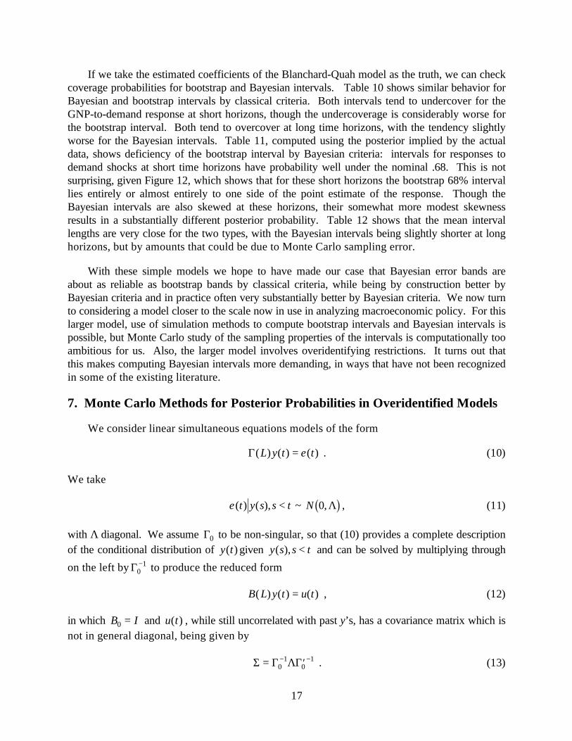
With these simple models we hope to have made our case that Bayesian error bands areabout as reliable as bootstrap bands by classical criteria, while being by construction better byBayesian criteria and in practice often very substantially better by Bayesian criteria. We now turnto considering a model closer to the scale now in use in analyzing macroeconomic policy. For thislarger model, use of simulation methods to compute bootstrap intervals and Bayesian intervals ispossible, but Monte Carlo study of the sampling properties of the intervals is computationally tooambitious for us. Also, the larger model involves overidentifying restrictions. It turns out thatthis makes computing Bayesian intervals more demanding, in ways that have not been recognizedin some of the existing literature.

7. Monte Carlo Methods for Posterior Probabilities in Overidentified Models

We consider linear simultaneous equations models of the form

Γ( ) ( ) ( )L y t t= ε . (10)

We take

ε ( ) ( ), ~ ,t y s s t N< 0 Λb g , (11)

with Λ diagonal. We assume Γ0 to be non-singular, so that (10) provides a complete descriptionof the conditional distribution of y t( ) given y s s t( ), < and can be solved by multiplying through

on the left by Γ01− to produce the reduced form

B L y t u t( ) ( ) ( )= , (12)

in which B I0 = and u t( ) , while still uncorrelated with past y’s, has a covariance matrix which isnot in general diagonal, being given by

Σ Γ ΛΓ= ′− −0

10

1 . (13)

18

We assume the system is a finite-order autoregression, meaning that there is a k < ∞ such thatΓ j jB= = 0 for all j k> .

The p.d.f. for the data y y T( ),..., ( )1 , conditional on the initial observationsy k y( ),..., ( )− +1 0 , is proportional to q as defined by

q B S BT

, expΣ Σ Σb g b gd i= − 2 - trace12

-1 (14)

$ ; ( ) ( )u t B B L y tb g = (15)

S B u t B u t Bt

T

( ) $( , ) $( , )= ′=∑

1

. (16)

For a given sample, (14) treated as a function of the parameters B and Σ is the likelihood function.Its form is exactly that of the likelihood for a regression with Gaussian disturbances and strictlyexogenous regressors, a classic model for which Bayesian calculations are well-discussed in theliterature.19 The RATS program includes routines to implement Monte Carlo drawing from thejoint distribution of B and Σ and use of those draws to generate a Monte Carlo sample from theposterior distribution of impulse responses.20

The impulse responses for the model , defined by (5) above, are in this case the coefficients of

B L− −10

1 12b gΓ Λ , (17)

where the Λ12 factor scales the structural disturbances to have unit variance, or equivalently

converts the responses so they have the scale of a response to a disturbance of “typical” (one-standard-deviation) size. Equation (13) gives us a relation among Σ, Γ, and Λ. Because Σ issymmetric, Γ0 and Λ have more unrestricted coefficients than Σ. An exactly identified VAR

19 See, e.g., Box and Tiao [1973], Chapter 8 for the theory.

20 Box and Tiao [1973] recommend using a Jeffreys prior on Σ, which turns out to be

proportional to Σ −+m 12 . The packaged RATS procedure uses instead Σ −

+ +m ν 12 , where ν is the

number of estimated coefficients per equation. Phillips [1992] suggests using the joint Jeffreysprior on B and Σ, which in time series models (unlike models with exogenous regressors) is notflat in B. The Phillips suggestion has the drawback that the joint Jeffreys prior is computationallyinconvenient and changes drastically with sample size, making it difficult for readers to compareresults across data sets. We therefore prefer the Box and Tiao suggestion in principle, thoughthey point out (p. 44) that even in models with exogenous regressors mechanical use of Jeffreyspriors can lead to anomalies. In this paper, to keep our results as comparable as possible to theexisting applied literature, we have followed the RATS procedure’s choice of prior.

19

model is one in which we have just enough restrictions available to make (13) a one-one mappingfrom Σ to Γ0 and Λ. In this case, sampling from the impulse responses defined by (17) isstraightforward: sample from the joint distribution of B and Σ by standard methods, then use themapping defined by (13) and the restrictions to convert these draws to draws from the distributionof impulse responses. The most common use of this procedure restricts Γ0 to be triangular,

solving for Γ Λ01 1

2− by taking a Choleski decomposition of Σ.

When the model is not exactly identified, however, reliance on the standard methods andprograms that generate draws from the joint distribution of the reduced form parameters is nolonger possible. A procedure with no small-sample rationale that does use the standard methodshas occurred independently to a number of researchers (including ourselves) and been used in atleast one published paper (Gordon and Leeper [1994]). We will call it the naive procedure.Because the method has a misleading intuitive appeal and may sometimes be easier to implementthan the correct method we describe below, we begin by describing it and explaining why itproduces neither a Bayesian posterior nor a classical sampling distribution.

In an overidentified model, (13) restricts the behavior of the true reduced-form innovationvariance matrix Σ. It remains true, though, that the OLS estimates $B and $Σ are sufficientstatistics, meaning that the likelihood depends on the data only through them. Thus maximumlikelihood estimation of B, Γ0 , and Λ implies an algorithm for mapping reduced form $ , $B Σd iestimates into structural estimates B∗ ∗ ∗, ,Γ Λ0d i that satisfy the restrictions Often there are no

restrictions that affect B, so that $B B= ∗ . The naive method proceeds by drawing from theunrestricted reduced form’s posterior p.d.f. for (B, Σ), then mapping these draws into values of

B, ,Γ Λ0b g via the maximum likelihood procedure, as if the parameter values drawn from theunrestricted posterior on (B, Σ) were instead reduced form parameter estimates. The resultingdistribution is of course concentrated on the part of the parameter space satisfying the restrictions,but is not a parametric bootstrap classical distribution for the parameter estimates, because theposterior distribution for (B, Σ) is not a sampling distribution for $ , $B Σd i . It is not a true posterior

distribution because the unrestricted posterior distribution for (B, Σ) is not the restricted posteriordistribution, and mapping it into the restricted parameter space via the estimation procedure doesnot convert it into a restricted posterior distribution.

The procedure does have the same sort of asymptotic justification that makes nearly allbootstrap and Bayesian methods of generating error bands asymptotically equivalent from aclassical point of view for stationary models, and it is probably asymptotically justified from aBayesian viewpoint as a normal approximation even for non-stationary models. To see this,consider a simple normal linear estimation problem, where we have a true parameter β, anunrestricted estimate distributed as N β ,Ωb g , and a restriction Rβ γ= with R k×m. Therestricted maximum likelihood estimate is then the projection on the Rβ γ= manifold of the

unrestricted ML estimate $β , under the metric defined by Ω, i.e.

20

$ $β β γ∗ − − − − −= ′ ′ + ′Φ Φ Ω Φ Φ Ω Ω1 1 1 1 1d i d iM M M , (18)

where M R= ′Ω and Φ is chosen to be of full column rank m-k and to satisfy RΦ = 0 . Thesampling distribution of $β∗ is then in turn normal, since it is a linear transformation of the normal$β . In this symmetrically distributed, pure location-shift problem, the unrestricted posterior on β

has the same normal p.d.f., centered at $β , as the sampling p.d.f. of $β about β. We could make

Monte Carlo draws from the sampling distribution of $β∗ by drawing from the sampling

distribution of $β , the unrestricted estimate, and projecting these unrestricted estimates on therestricted parameter space using the formula (18). But since in this case the posterior distributionof $β and its sampling distribution are the same, drawing from the posterior distribution in the firststep would give the same correct result. And since in this case the restricted posterior has thesame normal shape about $β∗ that the sampling distribution of $β∗ has about β, the simulateddistribution matches the posterior as well as the sampling distribution of the restricted estimate.

The naive method for sampling from the distribution of impulse responses rests on confusingsampling distributions with posterior distributions, but in the case of the preceding paragraph thiswould cause no harm, because the two kinds of distribution have the same shape. For stationarymodels, distribution theory for $Σ and $B is asymptotically normal, and differentiable restrictionswill behave asymptotically as if they were linear. So the case considered in the previousparagraph becomes a good approximation in large samples. For stationary or non-stationarymodels, the posterior on Σ is asymptotically normal, so the naive method is asymptoticallyjustified from a Bayesian point of view.

But in this paper we are focusing on methods that produce error bands whose possibleasymmetries are justifiably interpreted as informative about asymmetry in the posteriordistribution of the impulse responses or in the sampling distribution of their estimates. Anyasymmetries that appear in bands generated by the naive method are interpretable only as evidencethat the asymptotic approximations that might justify the method are not holding in the sample athand.

To describe a correct procedure for generating Monte Carlo draws from the Bayesianposterior for the parameters in (10), we begin by introducing a reparameterization. In place of(10) we use

A L y t t( ) ( ) ( )= η , (19)

where A = −Λ Γ12 and η ε( ) ( )t t= −Λ

12 so that var ( )η t Ib g = . There is no real reduction in the

number of free parameters, because the diagonal of Γ0 is always normalized to a vector of ones.so that an unrestricted A0 has the same number of parameters as a diagonal Λ together with anormalized Γ0 . There are a number of reasons to prefer this parameterization. It simplifies themapping (17) between reduced form and structural parameters. The usual parameterization can

21

give a misleading impression of imprecision in the estimate of a row of Γ0 if the normalizationhappens to set to 1 a particularly ill-determined coefficient in the corresponding row of A0 . Butthe main reason for introducing this parameterization here is that the likelihood is not in generalintegrable when written as a function of B, ,Γ Λ0b g , requiring some adjustment of the flat prior toallow formation of a posterior distribution, whereas it is integrable as a function of (B, A0 ).21

We can rewrite the likelihood (14) as

A A A S B B B X X B B A AT0 0 0 0 0

12

12

exp ( $ ( $) ( $)− ′ − − ′ ′ − ′RSTUVWtrace traced i d i . (20)

Taking the prior as flat in B and A0 , we can integrate over B to obtain the marginal posterior onA0 ,

p A A A S B AT( ) exp ( $)0 0 0 012

∝ − ′LNM

OQP

−ν traced i . (21)

Here as with the reduced-form model we have followed the widely used RATS code in droppingthe “degrees of freedom correction” -ν in (21), in effect using A0

ν as an improper prior. As canbe seen by comparing (20) with (21), this has the effect of making the marginal posterior on A0

proportional to the concentrated likelihood and thereby eliminating possible discrepanciesbetween posterior modes and maximum likelihood estimates.

Expression (21) is not in the form of any standard p.d.f. To generate Monte Carlo samplesfrom it, we first take a second-order Taylor expansion of it about its peak, which produces theusual Gaussian approximation to the asymptotic distribution of the elements of A0 . We draw asample from this distribution, but weight the draws by the ratio of (21) to the Gaussian p.d.f. from

21 In general, the likelihood, with B and Λ integrated out, is 0(1) in individual elements ofΓ0 at all sample sizes. This does not mean that it fails to be asymptotically normal -- thelikelihood does become small outside a region around the true parameter values. There are alsospecial cases where the likelihood is integrable, e.g. where Γ0 is normalized with ones down thediagonal and restricted to be triangular. For details, see the earlier draft of this paper, CowlesFoundation Discussion Paper No. 1085. Of course, we could use the standard parameterizationand retain integrability if we made the prior flat in A0 , then transformed back to the (Γ0 ,Λ)

parameter space, including the appropriate Jacobian term Λ −+m 12 . But the easiest way to explain

the appearance of this term would be to derive it from the A0 parameterization, which is in anycase more well-behaved.

22

which we draw. The weighted sample c.d.f. then approximates the c.d.f. corresponding to (21).22

The weights often vary rather widely, so that a given degree of Monte Carlo sampling error inimpulse response bands computed this way generally requires several times as many Monte Carlodraws as for a reduced form model where weighting is not required. Note that it also possible tocompute the error bands without any weighting. This is yet another example of a method forcomputing error bands that is asymptotically justified, but admits no rationale for interpreting itsasymmetries as providing information about small-sample deviations from normality.

Note that, though in switching to the A0 parameterization we have eliminated the need tochoose a normalization in the usual sense, there is still a discrete redundancy in theparameterization: the sign of a row of A0 can be reversed without changing the likelihoodfunction. We eliminate the redundancy by considering only A0 ’s with non-negative diagonalelements. Since the asymptotic approximation to the posterior on A0 is Gaussian, when we drawfrom it we generate some A0 ’s with negative diagonal elements. We simply discard such draws.23

8. Results for a Six-Variable Model

An earlier paper by one of us (Sims [1986]) contains an example of an overidentified VARmodel with an interesting interpretation. (It identifies a money supply shock that produces both aliquidity effect -- an initial decline in interest rate -- and a correct-signed price effect -- inflationfollowing a monetary expansion.) The paper contains two sets of identifying restrictions, and wehave computed error bands for both. One set is not displayed here, because it gave theuninteresting outcome that all non-bootstrap methods of computing error bands gave about thesame, symmetric, results, whether by correct Bayesian calculations, unweighted Bayesian MonteCarlo, or the naive method.24 It is worth noting that this can happen; one should not be satisfiedgenerally with the simpler methods of calculating error bands on the basis of a few test caseswhere more sophisticated calculations appear not to make a difference. The other version of themodel, called identification 2 in the original paper, produced substantial differences acrossmethods.

22 This idea, importance sampling, has seen wide use since its introduction into econometricsby Kloek and Van Dijk [1978].

23 If we retained such draws, flipping the sign on deviant rows of A0 , we would have torecognize that even when we have drawn an A0 with positive diagonal, the density of thedistribution from which we are drawing is not simply the Gaussian density at that point, but thesum of densities over all A0 ’s that map into that point via sign-reversals of diagonal elements.This seemed likely to slow down calculations by as much as does discarding the deviant draws.

24 Other-percentile method bootstrap intervals gave different results. We did not computebands by Killian’s method for this model.

23

Figure 11 shows impulse responses for this model, with .68 and .95 probability bandscomputed by the importance-sampling Bayesian Monte Carlo method. In all of Figures 11-13,longer-dashed lines are 95% bands and dotted lines are 68% bands. The .68 bands are tight inFigure 11, which makes the .95 bands useful.. The bands do not show much asymmetry, thoughthere is some, particularly for longer horizons and the .95 bands. For the model’s interpretation,the second column of the figure, which is identified as the responses to a money demand shock,are particularly interesting. Though most of them look like what would be expected of a moneydemand shock, the fourth, showing the response of the price level, may not be. It showsimmediate and strong inflation following the money demand increase.

This is not the place to discuss whether this discredits the model. (We are not sure it does.Equilibrium models can generate responses something like this to money demand shocks.) But itis clear that the price response is estimated as sharply positive, with very small probability of beingzero or negative. As we shall see, only this correct method of computing the posterior gives thissharp result.

Figure 12 shows responses to money supply and demand shocks with bands computed byseveral methods. The uncorrected other-percentile bootstrap shows strong bias, with the 68%band on the response of prices to money demand being very wide, not including the pointestimate, and nearly including the axis. The naive method produces even wider bands on thiscrucial response, again with the lower bound very close to the axis. The unweighted methodproduces somewhat narrower bands, but the 68% band still is skewed toward zero, close enoughthat it might suggest that the price response has at least a 2-3% chance of being zero in fact.Thus all three estimates fail to show the high precision with which this debatable response isactually estimated.

The bias-corrected bootstrap here produces bad results, as can be seen in Figure 13.Probably because of the severe bias apparent in the uncorrected bootstrap estimates in Figure 12,bias-correction as we have implemented it pushes the bootstrap distribution unreasonably far intothe nonstationary region and produces strongly asymmetric, rapidly explosive intervals that at afew points even fail to include point estimates. Like those in Figure 12, though, they are skeweddownward for the price-to-money-demand response and have a lower 68% limit that runs alongthe axis.

9. Computing Times

Forming 1000 draws from the posterior distribution for the impulse responses for our four-lag Y-M model, for example, takes less than 30 seconds using RATS code on a Pentium-90. Thesame is true for a bootstrap sample with a similar number of draws. For the six-variable model,the same calculation takes 2.13 minutes for the Bayesian interval and 3 minutes for the bootstrapinterval. To calculate equal-tailed intervals requires storing the draws and sorting the draws foreach a sij ( ) . This makes demands on sorting efficiency and on management of memory and diskstorage which we have not optimized very well. Replicating these calculations 600 times to getcoverage probabilities for the Y-M, for example, would take 5 hours for the other-percentilebootstrap, but our actual calculations took closer to 14 hours because of the need to sort andshuffle data on the disk. We think these times could be much reduced. Figure 11 is based on

24

20000 draws from the posterior, with 4936 of these discarded for negative diagonals. Figure 12is based on 1000 bootstrap draws. The bootstrap-after-bootstrap calculations for Figure 13 used1000 bootstrap draws in each layer of the bootstrap.

10. Conclusion

We have discussed the logical foundations of Bayesian and bootstrap inference for thesemodels and displayed the behavior of such intervals with actual and simulated data. We hope thishas led the reader to agree with us that posterior probability intervals are in principle more usefulthan confidence intervals and ought therefore to be the standard reporting device for these models(as in any other case where they differ from confidence intervals). Even readers who remainattached to the idea that only data, not parameters, can be given probability distributions ought tofind our results useful. They confirm that unadjusted other-percentile bootstrap intervals are farworse on classical criteria than Bayesian intervals. They also show that Bayesian intervals deserveattention even on purely classical criteria. Compared to carefully constructed bootstrap intervalsthey are computationally more efficient, similarly asymptotically justified, and similar on the wholein the accuracy of their small-sample coverage probabilities.

References

Blanchard, O.J. and D. Quah: “The Dynamic Effects of Aggregate Demand and SupplyDisturbances,” American Economic Review, 79(1989), 655-73

Box, G.E.P. and George Tiao: Bayesian Inference in Statistical Analysis. Addison-Wesley,1973.

Efron, Bradley and Robert J. Tibshirani: An Introduction to the Bootstrap, New York andLondon: Chapman and Hall, 1993.

Gordon, D.B. and E.M. Leeper: “The Dynamic Impacts of Monetary Policy: An Exercise inTentative Identification,” Journal of Political Economy , 102(1994), 1228-1247.

Hall, Peter: The Bootstrap and Edgeworth Expansion, Springer-Verlag, 1992.

Hildreth, Clifford: “Bayesian Statisticians and Remote Clients,” Econometrica, 31(1963),422-439.

Killian, Lutz: “Small-Sample Confidence Intervals for Impulse Response Functions,”processed, Department of Economics, University of Pennsylvania, 1995.

Kloek, T. and H.K. van Dijk: “Bayesian Estimates of Equation System Parameters: AnApplication of Integration by Monte Carlo,” Econometrica, 46(1978), 1-19.

Koop, G.: “Aggregate Shocks and Macroeconomic Fluctuations: A Bayesian Approach,”Journal of Appllied Econometrics, 7(1992), 395-411.

25

Lastrapes, W.D. and G. Selgin: “Buffer-Stock Money: Interpreting Short-Run DynamicsUsing Long-Run Restrictions,” Journal of Money, Credit and Banking, 26(1994), 34-54.

Lutkepohl, H.: “Asymptotic Distributions of Impulse Response Functions and Forecast ErrorVariance Decompositions of Vector Autoregressive Models,” The Review of Economics andStatistics, 72(1990), 53-78.

Mittnik, S. and P.A. Zadrozny: “Asymptotic Distributions of Impulse Responses, StepResponses, and Variance Decompositions of Estimated Linear Dynamic Models,” Econometrica,20(1993), 832-854.

Phillips, P.C.B.: “To Criticize the Critics: An Objective Bayesian Analysis of StochasticTrends,” Journal of Applied Econometrics, 7(1992).

Poterba, J.M., J.J. Rotemberg and L.H. Summers: “A Tax-Based Test for NominalRigidities,” American Economic Review, 76(1986), 659-675.

RATS, computer program available from Estima, 1800 Sherman Ave., Suite 612, EvanstonIL 60201.

Runkle, D.E.: “Vector Autoregressions and Reality,” Journal of Business and EconomicStatistics, 5(1987), 437-442.

Sims, C.A.: “Are Forecasting Models Usable for Policy Analysis?” Federal Reserve Bank ofMinneapolis Quarterly Review 10(1986), 2-15.

Sims, C., J. Stock and M. Watson: “Inference in Linear Time Series Models with Some UnitRoots,” Econometrica, 58(1989), 113-144.

Sims, C.A. and H. Uhlig: “Understanding Unit Rooters: A Helicopter Tour,” Econometrica,59(1991), 1591-1599.

26

Table 1

Classical Performance Criteria, Cointegrated ModelCoverage Probabilities for Bootstrap Intervals Coverage Probabilities for Bayesian Intervals

t 1 to 1 2 to 1 1 to 2 2 to 2 t 1 to 1 2 to 1 1 to 2 2 to 21 .582 .605 .000 .553 1 .663 .658 .000 .6582 .588 .617 .665 .653 2 .658 .660 .665 .6473 .603 .628 .660 .667 3 .670 .670 .668 .6574 .615 .623 .657 .662 4 .673 .678 .673 .6606 .623 .632 .652 .657 6 .677 .678 .670 .6658 .650 .635 .655 .653 8 .682 .683 .673 .677

12 .650 .645 .655 .652 12 .678 .680 .682 .67516 .662 .657 .653 .650 16 .677 .675 .682 .67724 .673 .668 .655 .652 24 .672 .680 .677 .67532 .692 .690 .657 .652 32 .675 .677 .680 .677

Note: Monte Carlo standard error of a .68 frequency with 600 draws is .019. Bootstrap intervalshave nominal coverage probability of .68. Bayesian intervals are flat-prior, equal-tail, .68posterior probability intervals.

27

Table 2

Bayesian Performance Criteria, Cointegrated Model

Sample 1 Sample 2t 1 to 1 2 to 1 1 to 2 2 to 2 t 1 to 1 2 to 1 1 to 2 2 to 21 .634 .624 .000 .594 1 .613 .604 .000 .6322 .629 .614 .621 .657 2 .622 .598 .692 .6713 .648 .634 .629 .657 3 .639 .616 .704 .6834 .673 .651 .640 .667 4 .670 .645 .707 .7126 .686 .694 .645 .683 6 .710 .685 .717 .7328 .694 .701 .652 .683 8 .723 .716 .726 .736

12 .715 .712 .667 .672 12 .750 .746 .744 .74816 .725 .726 .677 .675 16 .757 .752 .765 .75824 .717 .719 .680 .680 24 .787 .782 .768 .76432 .700 .707 .677 .677 32 .781 .776 .774 .771

Sample 3 Sample 4t 1 to 1 2 to 1 1 to 2 2 to 2 t 1 to 1 2 to 1 1 to 2 2 to 21 .602 .648 .000 .720 1 .576 .608 .000 .7002 .622 .645 .658 .650 2 .636 .637 .623 .6633 .659 .655 .660 .658 3 .649 .663 .609 .6734 .676 .689 .666 .675 4 .665 .673 .614 .6786 .702 .708 .677 .696 6 .676 .693 .606 .6348 .701 .724 .682 .699 8 .663 .678 .606 .626

12 .729 .733 .693 .698 12 .660 .669 .612 .61516 .749 .737 .703 .702 16 .669 .667 .618 .61724 .764 .762 .703 .708 24 .684 .682 .614 .61832 .780 .773 .696 .708 32 .698 .694 .614 .615

Note: Monte Carlo standard error of a .68 frequency with 1000 draws is .015. Bootstrapintervals have nominal coverage probability of .68. The samples are random draws with initial

y’s both 1, Ω =LNM

OQP

116 11 1.

, sample size 100. The four randomly drawn estimated coefficient

matrices were

Truth 1 2 3 4A' 0.9 0.1 1.060 .329 1.180 .355 1.174 .364 1.268 .536

0.1 0.9 -.058 .674 -.172 .654 -.165 .646 -.263 .473

c' 1 1 1.056 .987 .737 .769 .700 .718 1.006 .888

28

Table 3

Cointegrated ModelRatios of Interval LengthsBayesian over Bootstrap

t 1 to 1 2 to 1 1 to 2 2 to 21 1.044 1.040 1.000 1.0292 1.027 1.034 1.024 1.0283 1.014 1.023 .996 1.0094 .999 1.010 .973 .9866 .968 .980 .933 .9468 .941 .954 .901 .914

12 .900 .914 .853 .86416 .874 .885 .819 .82924 .847 .855 .776 .78432 .836 .843 .750 .755

Note: Monte Carlo standard errors of these ratios vary, but all are below .03.

Table 4

Classical Performance Criteria, Random Walks with DriftBootstrap Interval Coverage Probabilities Bayesian Interval Coverage Probabilities

t 1 to 1 2 to 1 1 to 2 2 to 2 t 1 to 1 2 to 1 1 to 2 2 to 21 .542 .688 .000 .510 1 .652 .640 .000 .6302 .460 .617 .535 .447 2 .530 .528 .295 .4803 .437 .575 .535 .427 3 .442 .433 .295 .3874 .453 .530 .535 .435 4 .377 .373 .295 .3306 .462 .503 .535 .442 6 .320 .320 .295 .2958 .470 .507 .535 .467 8 .287 .305 .295 .280

12 .482 .517 .535 .485 12 .282 .285 .295 .28216 .485 .517 .535 .497 16 .288 .288 .295 .28024 .500 .517 .535 .510 24 .278 .285 .295 .28332 .505 .527 .535 .520 32 .292 .283 .295 .295

Note: Monte Carlo standard error of a .68 frequency with 600 draws is .019. Bootstrap intervalshave nominal coverage probability of .68. Bayesian intervals are flat-prior, equal-tail, .68posterior probability intervals.

29

Table 5

Bayesian Performance Criteria, Random Walks with DriftPosterior Probability of Bootstrap Interval

t 1 to 1 2 to 1 1 to 2 2 to 21 .616 .618 .000 .5692 .677 .645 .568 .7073 .706 .640 .563 .7374 .713 .626 .567 .7226 .679 .628 .574 .7218 .660 .643 .581 .718

12 .672 .686 .632 .71516 .688 .715 .664 .76824 .741 .804 .696 .82332 .769 .851 .734 .860

A' .965 .061.036 .942

c' 1.170 .751

Note: Monte Carlo standard error of a .68 frequency with 1000 draws is .015. Bootstrapintervals have nominal coverage probability of .68. The samples are random draws with initial y’sboth 1.

Table 6

Random Walks with Drift

Ratios of Interval LengthsBayesian over Bootstrap

t 1 to 1 2 to 1 1 to 2 2 to 21 1.039 1.026 1.000 1.0272 .968 .963 .934 .9513 .916 .912 .905 .8984 .878 .873 .878 .8596 .819 .811 .830 .8038 .771 .762 .787 .758

12 .688 .680 .707 .67916 .611 .603 .632 .60624 .461 .450 .484 .46132 .313 .304 .336 .319

Note: Monte Carlo standard errors of these ratios vary, but all are below .06.

30

Table 7

Classical Performance Criteria, GNP-M1 ModelBootstrap Interval Coverage Probabilities Bayesian Interval Coverage Probabilities

Y to Y M to Y Y to M M to M t Y to Y M to Y Y to M M to M.432 .687 .000 .360 1 .595 .668 .000 .595.540 .678 .717 .502 2 .618 .672 .685 .543.603 .692 .685 .592 3 .577 .687 .643 .557.625 .670 .688 .622 4 .593 .690 .613 .518.657 .702 .687 .653 6 .585 .677 .618 .523.650 .713 .685 .655 8 .560 .670 .610 .510.682 .717 .697 .675 12 .555 .642 .627 .518.703 .732 .707 .687 16 .557 .623 .608 .513.712 .730 .742 .712 24 .570 .642 .617 .517.725 .742 .748 .750 32 .602 .632 .610 .520

Note: Monte Carlo standard error of a .68 frequency with 600 draws is .019. Bootstrap intervalshave nominal coverage probability of .68. Bayesian intervals are flat-prior, equal-tail, .68posterior probability intervals.

Table 8

Bayesian Performance Criteria, GNP-M1 ModelPosterior Probability of Bootstrap Interval

t Y to Y M to Y Y to M M to M1 .613 .685 .000 .8092 .723 .722 .680 .7993 .716 .697 .683 .7804 .742 .713 .678 .7606 .729 .751 .732 .7258 .726 .769 .765 .702

12 .778 .790 .818 .67116 .788 .822 .841 .67524 .801 .831 .868 .71632 .809 .832 .883 .776

Note: Monte Carlo standard error of a .68 frequency with 1000 draws is .015. Bootstrapintervals have nominal coverage probability of .68. The samples are random draws with initial y’sboth 1.

31

Table 9

GNP-M1 ModelRatios of Mean Lengths: Bayesian/Bootstrap

t Y to Y M to Y Y to M M to M1 1.022 1.016 1.000 1.0202 .995 .988 1.015 .9833 .967 .961 .982 .9494 .938 .929 .945 .9186 .895 .880 .892 .8728 .841 .829 .836 .828

12 .759 .762 .750 .75616 .716 .730 .708 .72124 .652 .691 .644 .67732 .603 .661 .599 .647

Table 10

Classical Performance Criteria, Blanchard-Quah ModelBootstrap Interval Coverage Probabilities Bayesian Interval Coverage Probabilities

t Y to S U to S Y to D U to D t Y to S U to S Y to D U to D1 .657 .650 .050 .632 1 .653 .662 .273 .6722 .648 .653 .108 .425 2 .658 .655 .270 .6183 .647 .642 .225 .295 3 .650 .668 .372 .4624 .657 .642 .337 .297 4 .658 .660 .445 .4486 .678 .647 .550 .452 6 .642 .637 .615 .5058 .670 .672 .593 .525 8 .647 .623 .652 .600

12 .687 .705 .630 .635 12 .690 .705 .658 .63216 .728 .775 .645 .707 16 .752 .792 .693 .72524 .747 .845 .783 .780 24 .768 .860 .845 .85332 .737 .910 .928 .865 32 .760 .923 .952 .920

Note: Monte Carlo standard error of a .68 frequency with 600 draws is .019. Bootstrap intervalshave nominal coverage probability of .68. Bayesian intervals are flat-prior, equal-tail, .68posterior probability intervals.

32

Table 11

Bayesian Performance Criteria, Blanchard-Quah ModelPosterior Probabilities of Bootstrap Intervals

t Y to S U to S Y to D U to D1 .710 .696 .452 .6442 .706 .715 .583 .6163 .701 .717 .655 .6114 .688 .712 .700 .6616 .693 .696 .712 .6738 .703 .698 .705 .731

12 .687 .718 .700 .69216 .693 .713 .689 .68424 .668 .714 .670 .67632 .655 .721 .707 .718

Note: Monte Carlo standard error of a .68 frequency with 1000 draws is .015. Bootstrapintervals have nominal coverage probability of .68. The samples are random draws with initial y’sboth 1.

Table 12

Blanchard-Quah ModelRatios of Mean Lengths: Bayesian/Bootstrap

t Y to S U to S Y to D U to D1 1.009 1.004 .996 1.0082 1.005 1.001 .985 1.0063 .997 .999 .979 .9934 .990 .992 .979 .9846 .972 .981 .997 .9848 .962 .975 .991 .994

12 .972 .985 .995 .99916 .979 .983 1.005 1.01624 .976 .942 .984 1.00132 .963 .886 .958 .969

Note: Monte Carlo standard errors of these figures vary, but none are over .06.

33

Figure 1

Example 2 p.d.f. for µµ = 0 and µµ = 1

Figure 2Example 2 Likelihood, X = 1

µ

µ=1

µ=0

X→

34

Figure 3Example 3 p.d.f. for µµ=1 and µµ=1/e

µ=1/e

µ=1

X→

Figure 4Example 3 Likelihood for X=1

µ→

35

Figure 5

68% and 98% Other-Percentile Bootstrap Bands, Y-M Model

Responses to Y Responses to M

Y

M

36

Figure 6

.68 and .95 Posterior Probability Bands, Y-M Model

Responses to Y Responses to M

2 8 14 20 260.0050

0.0075

0.0100

0.0125

0.0150

0.0175

0.0200

0.0225

2 8 14 20 26-0.0050

-0.0025

0.0000

0.0025

0.0050

0.0075

0.0100

0.0125

0.0150

0.0175

2 8 14 20 26-0.002

0.000

0.002

0.004

0.006

0.008

0.010

0.012

0.014

2 8 14 20 260.005

0.010

0.015

0.020

0.025

0.030

Y

M

37

Figure 7

68% and 95% Bias-Corrected Bootstrap Bands, Y-M Model

Responses to Y Responses to M

2 8 14 20 260.000

0.005

0.010

0.015

0.020

0.025

0.030

2 8 14 20 26-0.015

-0.010

-0.005

0.000

0.005

0.010

0.015

0.020

2 8 14 20 26-0.0075

-0.0050

-0.0025

0.0000

0.0025

0.0050

0.0075

0.0100

0.0125

0.0150

2 8 14 20 260.005

0.010

0.015

0.020

0.025

0.030

0.035

0.040

Y

M

38

Figure 8

68% and 95% Other-Percentile Bootstrap Bands, B-Q Model

Responses to Supply Responses to Demand

2 9 16 23 30 37-1.0

-0.5

0.0

0.5

1.0

1.5

2 9 16 23 30 37-0.4

-0.2

0.0

0.2

0.4

0.6

2 9 16 23 30 37-0.25

0.00

0.25

0.50

0.75

1.00

1.25

1.50

2 9 16 23 30 37-0.7

-0.6

-0.5

-0.4

-0.3

-0.2

-0.1

-0.0

0.1

0.2

Y

U

39

Figure 9

.68 and .95 Posterior Probability Bands, B-Q Model

Responses to Supply Responses to Demand

2 9 16 23 30 37-1.0

-0.5

0.0

0.5

1.0

1.5

2.0

2 9 16 23 30 37-0.50

-0.25

0.00

0.25

0.50

0.75

2 9 16 23 30 37-0.50

-0.25

0.00

0.25

0.50

0.75

1.00

1.25

1.50

1.75

2 9 16 23 30 37-0.75

-0.50

-0.25

0.00

0.25

U

Y

40

Figure 10

68% and 95% Bias-Corrected Bootstrap Bands, B-Q Model

Responses to Supply Responses to Demand

2 9 16 23 30 37-1.0

-0.5

0.0

0.5

1.0

1.5

2 9 16 23 30 37-0.4

-0.2

0.0

0.2

0.4

0.6

2 9 16 23 30 37-0.25

0.00

0.25

0.50

0.75

1.00

1.25

1.50

2 9 16 23 30 37-0.7

-0.6

-0.5

-0.4

-0.3

-0.2

-0.1

-0.0

0.1

Y

U

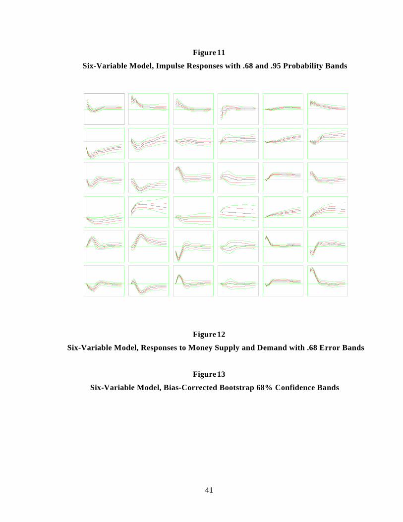
41

Figure 11

Six-Variable Model, Impulse Responses with .68 and .95 Probability Bands

Figure 12

Six-Variable Model, Responses to Money Supply and Demand with .68 Error Bands

Figure 13

Six-Variable Model, Bias-Corrected Bootstrap 68% Confidence Bands