Embed Size (px)
Citation preview
Error-correcting codes and cryptology
Ruud Pellikaan 1,Xin-Wen Wu 2,
Stanislav Bulygin 3 andRelinde Jurrius 4
PRELIMINARY VERSION23 January 2012
All rights reserved.To be published by Cambridge University Press.No part of this manuscript is to be reproduced
without written consent of the authors and the publisher.
[email protected], Department of Mathematics and Computing Science, Eind-hoven University of Technology, P.O. Box 513, NL-5600 MB Eindhoven, The Nether-lands
[email protected], School of Information and Communication Technology, Grif-fith University, Gold Coast, QLD 4222, Australia
[email protected], Department of Mathematics, Technische UniversitatDarmstadt, Mornewegstrasse 32, 64293 Darmstadt, Germany
[email protected], Department of Mathematics and Computing Science, Eind-hoven University of Technology, P.O. Box 513, NL-5600 MB Eindhoven, The Nether-lands

2
Contents
1 Introduction 111.1 Notes . . . . . . . . . . . . . . . . . . . . . . . . . . . . . . . . . 11
2 Error-correcting codes 132.1 Block codes . . . . . . . . . . . . . . . . . . . . . . . . . . . . . . 14
2.1.1 Repetition, product and Hamming codes . . . . . . . . . . 152.1.2 Codes and Hamming distance . . . . . . . . . . . . . . . . 182.1.3 Exercises . . . . . . . . . . . . . . . . . . . . . . . . . . . 21
2.2 Linear Codes . . . . . . . . . . . . . . . . . . . . . . . . . . . . . 212.2.1 Linear codes . . . . . . . . . . . . . . . . . . . . . . . . . 212.2.2 Generator matrix and systematic encoding . . . . . . . . 222.2.3 Exercises . . . . . . . . . . . . . . . . . . . . . . . . . . . 25
2.3 Parity checks and dual code . . . . . . . . . . . . . . . . . . . . . 262.3.1 Parity check matrix . . . . . . . . . . . . . . . . . . . . . 262.3.2 Hamming and simplex codes . . . . . . . . . . . . . . . . 282.3.3 Inner product and dual codes . . . . . . . . . . . . . . . . 302.3.4 Exercises . . . . . . . . . . . . . . . . . . . . . . . . . . . 32
2.4 Decoding and the error probability . . . . . . . . . . . . . . . . . 332.4.1 Decoding problem . . . . . . . . . . . . . . . . . . . . . . 342.4.2 Symmetric channel . . . . . . . . . . . . . . . . . . . . . . 352.4.3 Exercises . . . . . . . . . . . . . . . . . . . . . . . . . . . 38
2.5 Equivalent codes . . . . . . . . . . . . . . . . . . . . . . . . . . . 382.5.1 Number of generator matrices and codes . . . . . . . . . . 382.5.2 Isometries and equivalent codes . . . . . . . . . . . . . . . 402.5.3 Exercises . . . . . . . . . . . . . . . . . . . . . . . . . . . 44
2.6 Notes . . . . . . . . . . . . . . . . . . . . . . . . . . . . . . . . . 45
3 Code constructions and bounds 473.1 Code constructions . . . . . . . . . . . . . . . . . . . . . . . . . . 47
3.1.1 Constructing shorter and longer codes . . . . . . . . . . . 473.1.2 Product codes . . . . . . . . . . . . . . . . . . . . . . . . 523.1.3 Several sum constructions . . . . . . . . . . . . . . . . . . 553.1.4 Concatenated codes . . . . . . . . . . . . . . . . . . . . . 603.1.5 Exercises . . . . . . . . . . . . . . . . . . . . . . . . . . . 62
3.2 Bounds on codes . . . . . . . . . . . . . . . . . . . . . . . . . . . 633.2.1 Singleton bound and MDS codes . . . . . . . . . . . . . . 633.2.2 Griesmer bound . . . . . . . . . . . . . . . . . . . . . . . 683.2.3 Hamming bound . . . . . . . . . . . . . . . . . . . . . . . 69
3
4 CONTENTS
3.2.4 Plotkin bound . . . . . . . . . . . . . . . . . . . . . . . . 713.2.5 Gilbert and Varshamov bounds . . . . . . . . . . . . . . . 723.2.6 Exercises . . . . . . . . . . . . . . . . . . . . . . . . . . . 73
3.3 Asymptotically good codes . . . . . . . . . . . . . . . . . . . . . 743.3.1 Asymptotic Gibert-Varshamov bound . . . . . . . . . . . 743.3.2 Some results for the generic case . . . . . . . . . . . . . . 773.3.3 Exercises . . . . . . . . . . . . . . . . . . . . . . . . . . . 78
3.4 Notes . . . . . . . . . . . . . . . . . . . . . . . . . . . . . . . . . 78
4 Weight enumerator 794.1 Weight enumerator . . . . . . . . . . . . . . . . . . . . . . . . . . 79
4.1.1 Weight spectrum . . . . . . . . . . . . . . . . . . . . . . . 794.1.2 Average weight enumerator . . . . . . . . . . . . . . . . . 834.1.3 MacWilliams identity . . . . . . . . . . . . . . . . . . . . 854.1.4 Exercises . . . . . . . . . . . . . . . . . . . . . . . . . . . 88
4.2 Error probability . . . . . . . . . . . . . . . . . . . . . . . . . . . 884.2.1 Error probability of undetected error . . . . . . . . . . . . 894.2.2 Probability of decoding error . . . . . . . . . . . . . . . . 894.2.3 Random coding . . . . . . . . . . . . . . . . . . . . . . . . 904.2.4 Exercises . . . . . . . . . . . . . . . . . . . . . . . . . . . 90
4.3 Finite geometry and codes . . . . . . . . . . . . . . . . . . . . . . 904.3.1 Projective space and projective systems . . . . . . . . . . 904.3.2 MDS codes and points in general position . . . . . . . . . 954.3.3 Exercises . . . . . . . . . . . . . . . . . . . . . . . . . . . 97
4.4 Extended weight enumerator . . . . . . . . . . . . . . . . . . . . 974.4.1 Arrangements of hyperplanes . . . . . . . . . . . . . . . . 974.4.2 Weight distribution of MDS codes . . . . . . . . . . . . . 1024.4.3 Extended weight enumerator . . . . . . . . . . . . . . . . 1044.4.4 Puncturing and shortening . . . . . . . . . . . . . . . . . 1074.4.5 Exercises . . . . . . . . . . . . . . . . . . . . . . . . . . . 110
4.5 Generalized weight enumerator . . . . . . . . . . . . . . . . . . . 1114.5.1 Generalized Hamming weights . . . . . . . . . . . . . . . 1114.5.2 Generalized weight enumerators . . . . . . . . . . . . . . . 1134.5.3 Generalized weight enumerators of MDS-codes . . . . . . 1154.5.4 Connections . . . . . . . . . . . . . . . . . . . . . . . . . . 1184.5.5 Exercises . . . . . . . . . . . . . . . . . . . . . . . . . . . 120
4.6 Notes . . . . . . . . . . . . . . . . . . . . . . . . . . . . . . . . . 120
5 Codes and related structures 1235.1 Graphs and codes . . . . . . . . . . . . . . . . . . . . . . . . . . . 123
5.1.1 Colorings of a graph . . . . . . . . . . . . . . . . . . . . . 1235.1.2 Codes on graphs . . . . . . . . . . . . . . . . . . . . . . . 1265.1.3 Exercises . . . . . . . . . . . . . . . . . . . . . . . . . . . 127
5.2 Matroids and codes . . . . . . . . . . . . . . . . . . . . . . . . . . 1285.2.1 Matroids . . . . . . . . . . . . . . . . . . . . . . . . . . . 1285.2.2 Realizable matroids . . . . . . . . . . . . . . . . . . . . . 1295.2.3 Graphs and matroids . . . . . . . . . . . . . . . . . . . . . 1305.2.4 Tutte and Whitney polynomial of a matroid . . . . . . . . 1315.2.5 Weight enumerator and Tutte polynomial . . . . . . . . . 1325.2.6 Deletion and contraction of matroids . . . . . . . . . . . . 133
CONTENTS 5
5.2.7 McWilliams type property for duality . . . . . . . . . . . 1345.2.8 Exercises . . . . . . . . . . . . . . . . . . . . . . . . . . . 136
5.3 Geometric lattices and codes . . . . . . . . . . . . . . . . . . . . 1365.3.1 Posets, the Mobius function and lattices . . . . . . . . . . 1365.3.2 Geometric lattices . . . . . . . . . . . . . . . . . . . . . . 1415.3.3 Geometric lattices and matroids . . . . . . . . . . . . . . 1445.3.4 Exercises . . . . . . . . . . . . . . . . . . . . . . . . . . . 145
5.4 Characteristic polynomial . . . . . . . . . . . . . . . . . . . . . . 1465.4.1 Characteristic and Mobius polynomial . . . . . . . . . . . 1465.4.2 Characteristic polynomial of an arrangement . . . . . . . 1485.4.3 Characteristic polynomial of a code . . . . . . . . . . . . 1505.4.4 Minimal codewords and subcodes . . . . . . . . . . . . . . 1565.4.5 Two variable zeta function . . . . . . . . . . . . . . . . . 1575.4.6 Overview . . . . . . . . . . . . . . . . . . . . . . . . . . . 1575.4.7 Exercises . . . . . . . . . . . . . . . . . . . . . . . . . . . 158
5.5 Combinatorics and codes . . . . . . . . . . . . . . . . . . . . . . . 1585.5.1 Orthogonal arrays and codes . . . . . . . . . . . . . . . . 1585.5.2 Designs and codes . . . . . . . . . . . . . . . . . . . . . . 1615.5.3 Exercises . . . . . . . . . . . . . . . . . . . . . . . . . . . 161
5.6 Notes . . . . . . . . . . . . . . . . . . . . . . . . . . . . . . . . . 162
6 Complexity and decoding 1656.1 Complexity . . . . . . . . . . . . . . . . . . . . . . . . . . . . . . 165
6.1.1 Big-Oh notation . . . . . . . . . . . . . . . . . . . . . . . 1656.1.2 Boolean functions . . . . . . . . . . . . . . . . . . . . . . 1666.1.3 Hard problems . . . . . . . . . . . . . . . . . . . . . . . . 1716.1.4 Exercises . . . . . . . . . . . . . . . . . . . . . . . . . . . 172
6.2 Decoding . . . . . . . . . . . . . . . . . . . . . . . . . . . . . . . 1736.2.1 Decoding complexity . . . . . . . . . . . . . . . . . . . . . 1736.2.2 Decoding erasures . . . . . . . . . . . . . . . . . . . . . . 1746.2.3 Information and covering set decoding . . . . . . . . . . . 1776.2.4 Nearest neighbor decoding . . . . . . . . . . . . . . . . . . 1846.2.5 Exercises . . . . . . . . . . . . . . . . . . . . . . . . . . . 184
6.3 Difficult problems in coding theory . . . . . . . . . . . . . . . . . 1846.3.1 General decoding and computing minimum distance . . . 1846.3.2 Is decoding up to half the minimum distance hard? . . . . 1876.3.3 Other hard problems . . . . . . . . . . . . . . . . . . . . . 188
6.4 Notes . . . . . . . . . . . . . . . . . . . . . . . . . . . . . . . . . 188
7 Cyclic codes 1897.1 Cyclic codes . . . . . . . . . . . . . . . . . . . . . . . . . . . . . . 189
7.1.1 Definition of cyclic codes . . . . . . . . . . . . . . . . . . 1897.1.2 Cyclic codes as ideals . . . . . . . . . . . . . . . . . . . . 1917.1.3 Generator polynomial . . . . . . . . . . . . . . . . . . . . 1927.1.4 Encoding cyclic codes . . . . . . . . . . . . . . . . . . . . 1957.1.5 Reversible codes . . . . . . . . . . . . . . . . . . . . . . . 1967.1.6 Parity check polynomial . . . . . . . . . . . . . . . . . . . 1977.1.7 Exercises . . . . . . . . . . . . . . . . . . . . . . . . . . . 200
7.2 Defining zeros . . . . . . . . . . . . . . . . . . . . . . . . . . . . . 2017.2.1 Structure of finite fields . . . . . . . . . . . . . . . . . . . 201
6 CONTENTS
7.2.2 Minimal polynomials . . . . . . . . . . . . . . . . . . . . . 205
7.2.3 Cyclotomic polynomials and cosets . . . . . . . . . . . . . 206
7.2.4 Zeros of the generator polynomial . . . . . . . . . . . . . 211
7.2.5 Exercises . . . . . . . . . . . . . . . . . . . . . . . . . . . 213
7.3 Bounds on the minimum distance . . . . . . . . . . . . . . . . . . 214
7.3.1 BCH bound . . . . . . . . . . . . . . . . . . . . . . . . . . 214
7.3.2 Quadratic residue codes . . . . . . . . . . . . . . . . . . . 217
7.3.3 Hamming, simplex and Golay codes as cyclic codes . . . . 217
7.3.4 Exercises . . . . . . . . . . . . . . . . . . . . . . . . . . . 218
7.4 Improvements of the BCH bound . . . . . . . . . . . . . . . . . . 219
7.4.1 Hartmann-Tzeng bound . . . . . . . . . . . . . . . . . . . 219
7.4.2 Roos bound . . . . . . . . . . . . . . . . . . . . . . . . . . 220
7.4.3 AB bound . . . . . . . . . . . . . . . . . . . . . . . . . . . 223
7.4.4 Shift bound . . . . . . . . . . . . . . . . . . . . . . . . . . 224
7.4.5 Exercises . . . . . . . . . . . . . . . . . . . . . . . . . . . 228
7.5 Locator polynomials and decoding cyclic codes . . . . . . . . . . 229
7.5.1 Mattson-Solomon polynomial . . . . . . . . . . . . . . . . 229
7.5.2 Newton identities . . . . . . . . . . . . . . . . . . . . . . . 230
7.5.3 APGZ algorithm . . . . . . . . . . . . . . . . . . . . . . . 232
7.5.4 Closed formulas . . . . . . . . . . . . . . . . . . . . . . . . 234
7.5.5 Key equation and Forney’s formula . . . . . . . . . . . . . 235
7.5.6 Exercises . . . . . . . . . . . . . . . . . . . . . . . . . . . 238
7.6 Notes . . . . . . . . . . . . . . . . . . . . . . . . . . . . . . . . . 239
8 Polynomial codes 241
8.1 RS codes and their generalizations . . . . . . . . . . . . . . . . . 241
8.1.1 Reed-Solomon codes . . . . . . . . . . . . . . . . . . . . . 241
8.1.2 Extended and generalized RS codes . . . . . . . . . . . . 243
8.1.3 GRS codes under transformations . . . . . . . . . . . . . 247
8.1.4 Exercises . . . . . . . . . . . . . . . . . . . . . . . . . . . 250
8.2 Subfield and trace codes . . . . . . . . . . . . . . . . . . . . . . . 251
8.2.1 Restriction and extension by scalars . . . . . . . . . . . . 251
8.2.2 Parity check matrix of a restricted code . . . . . . . . . . 252
8.2.3 Invariant subspaces . . . . . . . . . . . . . . . . . . . . . . 254
8.2.4 Cyclic codes as subfield subcodes . . . . . . . . . . . . . . 257
8.2.5 Trace codes . . . . . . . . . . . . . . . . . . . . . . . . . . 258
8.2.6 Exercises . . . . . . . . . . . . . . . . . . . . . . . . . . . 258
8.3 Some families of polynomial codes . . . . . . . . . . . . . . . . . 259
8.3.1 Alternant codes . . . . . . . . . . . . . . . . . . . . . . . . 259
8.3.2 Goppa codes . . . . . . . . . . . . . . . . . . . . . . . . . 260
8.3.3 Counting polynomials . . . . . . . . . . . . . . . . . . . . 263
8.3.4 Exercises . . . . . . . . . . . . . . . . . . . . . . . . . . . 265
8.4 Reed-Muller codes . . . . . . . . . . . . . . . . . . . . . . . . . . 266
8.4.1 Punctured Reed-Muller codes as cyclic codes . . . . . . . 266
8.4.2 Reed-Muller codes as subfield subcodes and trace codes . 267
8.4.3 Exercises . . . . . . . . . . . . . . . . . . . . . . . . . . . 270
8.5 Notes . . . . . . . . . . . . . . . . . . . . . . . . . . . . . . . . . 270
CONTENTS 7
9 Algebraic decoding 2719.1 Error-correcting pairs . . . . . . . . . . . . . . . . . . . . . . . . 271
9.1.1 Decoding by error-correcting pairs . . . . . . . . . . . . . 2719.1.2 Existence of error-correcting pairs . . . . . . . . . . . . . 2759.1.3 Exercises . . . . . . . . . . . . . . . . . . . . . . . . . . . 276
9.2 Decoding by key equation . . . . . . . . . . . . . . . . . . . . . . 2779.2.1 Algorithm of Euclid-Sugiyama . . . . . . . . . . . . . . . 2779.2.2 Algorithm of Berlekamp-Massey . . . . . . . . . . . . . . 2789.2.3 Exercises . . . . . . . . . . . . . . . . . . . . . . . . . . . 281
9.3 List decoding by Sudan’s algorithm . . . . . . . . . . . . . . . . . 2819.3.1 Error-correcting capacity . . . . . . . . . . . . . . . . . . 2829.3.2 Sudan’s algorithm . . . . . . . . . . . . . . . . . . . . . . 2859.3.3 List decoding of Reed-Solomon codes . . . . . . . . . . . . 2879.3.4 List Decoding of Reed-Muller codes . . . . . . . . . . . . 2919.3.5 Exercises . . . . . . . . . . . . . . . . . . . . . . . . . . . 292
9.4 Notes . . . . . . . . . . . . . . . . . . . . . . . . . . . . . . . . . 292
10 Cryptography 29510.1 Symmetric cryptography and block ciphers . . . . . . . . . . . . 295
10.1.1 Symmetric cryptography . . . . . . . . . . . . . . . . . . . 29510.1.2 Block ciphers. Simple examples . . . . . . . . . . . . . . . 29610.1.3 Security issues . . . . . . . . . . . . . . . . . . . . . . . . 30010.1.4 Modern ciphers. DES and AES . . . . . . . . . . . . . . . 30210.1.5 Exercises . . . . . . . . . . . . . . . . . . . . . . . . . . . 308
10.2 Asymmetric cryptosystems . . . . . . . . . . . . . . . . . . . . . 30810.2.1 RSA . . . . . . . . . . . . . . . . . . . . . . . . . . . . . . 31110.2.2 Discrete logarithm problem and public-key cryptography 31410.2.3 Some other asymmetric cryptosystems . . . . . . . . . . . 31610.2.4 Exercises . . . . . . . . . . . . . . . . . . . . . . . . . . . 317
10.3 Authentication, orthogonal arrays, and codes . . . . . . . . . . . 31710.3.1 Authentication codes . . . . . . . . . . . . . . . . . . . . . 31710.3.2 Authentication codes and other combinatorial objects . . 32110.3.3 Exercises . . . . . . . . . . . . . . . . . . . . . . . . . . . 324
10.4 Secret sharing . . . . . . . . . . . . . . . . . . . . . . . . . . . . . 32410.4.1 Exercises . . . . . . . . . . . . . . . . . . . . . . . . . . . 328
10.5 Basics of stream ciphers. Linear feedback shift registers . . . . . 32910.5.1 Exercises . . . . . . . . . . . . . . . . . . . . . . . . . . . 334
10.6 PKC systems using error-correcting codes . . . . . . . . . . . . . 33510.6.1 McEliece encryption scheme . . . . . . . . . . . . . . . . . 33610.6.2 Niederreiter’s encryption scheme . . . . . . . . . . . . . . 33810.6.3 Attacks . . . . . . . . . . . . . . . . . . . . . . . . . . . . 34010.6.4 The attack of Sidelnikov and Shestakov . . . . . . . . . . 34310.6.5 Exercises . . . . . . . . . . . . . . . . . . . . . . . . . . . 344
10.7 Notes . . . . . . . . . . . . . . . . . . . . . . . . . . . . . . . . . 34510.7.1 Section 10.1 . . . . . . . . . . . . . . . . . . . . . . . . . . 34510.7.2 Section 10.2 . . . . . . . . . . . . . . . . . . . . . . . . . . 34710.7.3 Section 10.3 . . . . . . . . . . . . . . . . . . . . . . . . . . 34810.7.4 Section 10.4 . . . . . . . . . . . . . . . . . . . . . . . . . . 34810.7.5 Section 10.5 . . . . . . . . . . . . . . . . . . . . . . . . . . 34910.7.6 Section 10.6 . . . . . . . . . . . . . . . . . . . . . . . . . . 349
8 CONTENTS
11 The theory of Grobner bases and its applications 35111.1 Polynomial system solving . . . . . . . . . . . . . . . . . . . . . . 352
11.1.1 Linearization techniques . . . . . . . . . . . . . . . . . . . 35211.1.2 Grobner bases . . . . . . . . . . . . . . . . . . . . . . . . 35511.1.3 Exercises . . . . . . . . . . . . . . . . . . . . . . . . . . . 362
11.2 Decoding codes with Grobner bases . . . . . . . . . . . . . . . . . 36311.2.1 Cooper’s philosophy . . . . . . . . . . . . . . . . . . . . . 36311.2.2 Newton identities based method . . . . . . . . . . . . . . 36811.2.3 Decoding arbitrary linear codes . . . . . . . . . . . . . . . 37111.2.4 Exercises . . . . . . . . . . . . . . . . . . . . . . . . . . . 373
11.3 Algebraic cryptanalysis . . . . . . . . . . . . . . . . . . . . . . . 37411.3.1 Toy example . . . . . . . . . . . . . . . . . . . . . . . . . 37411.3.2 Writing down equations . . . . . . . . . . . . . . . . . . . 37511.3.3 General S-Boxes . . . . . . . . . . . . . . . . . . . . . . . 37811.3.4 Exercises . . . . . . . . . . . . . . . . . . . . . . . . . . . 379
11.4 Notes . . . . . . . . . . . . . . . . . . . . . . . . . . . . . . . . . 380
12 Coding theory with computer algebra packages 38112.1 Singular . . . . . . . . . . . . . . . . . . . . . . . . . . . . . . . . 38112.2 Magma . . . . . . . . . . . . . . . . . . . . . . . . . . . . . . . . 383
12.2.1 Linear codes . . . . . . . . . . . . . . . . . . . . . . . . . 38412.2.2 AG-codes . . . . . . . . . . . . . . . . . . . . . . . . . . . 38512.2.3 Algebraic curves . . . . . . . . . . . . . . . . . . . . . . . 385
12.3 GAP . . . . . . . . . . . . . . . . . . . . . . . . . . . . . . . . . . 38612.4 Sage . . . . . . . . . . . . . . . . . . . . . . . . . . . . . . . . . . 387
12.4.1 Coding Theory . . . . . . . . . . . . . . . . . . . . . . . . 38712.4.2 Cryptography . . . . . . . . . . . . . . . . . . . . . . . . . 38812.4.3 Algebraic curves . . . . . . . . . . . . . . . . . . . . . . . 388
12.5 Coding with computer algebra . . . . . . . . . . . . . . . . . . . 38812.5.1 Introduction . . . . . . . . . . . . . . . . . . . . . . . . . 38812.5.2 Error-correcting codes . . . . . . . . . . . . . . . . . . . . 38812.5.3 Code constructions and bounds . . . . . . . . . . . . . . . 39212.5.4 Weight enumerator . . . . . . . . . . . . . . . . . . . . . . 39512.5.5 Codes and related structures . . . . . . . . . . . . . . . . 39712.5.6 Complexity and decoding . . . . . . . . . . . . . . . . . . 39712.5.7 Cyclic codes . . . . . . . . . . . . . . . . . . . . . . . . . . 39712.5.8 Polynomial codes . . . . . . . . . . . . . . . . . . . . . . . 39912.5.9 Algebraic decoding . . . . . . . . . . . . . . . . . . . . . . 401
13 Bezout’s theorem and codes on plane curves 40313.1 Affine and projective space . . . . . . . . . . . . . . . . . . . . . 40313.2 Plane curves . . . . . . . . . . . . . . . . . . . . . . . . . . . . . . 40313.3 Bezout’s theorem . . . . . . . . . . . . . . . . . . . . . . . . . . . 406
13.3.1 Another proof of Bezout’s theorem by the footprint . . . 41313.4 Codes on plane curves . . . . . . . . . . . . . . . . . . . . . . . . 41313.5 Conics, arcs and Segre . . . . . . . . . . . . . . . . . . . . . . . . 41413.6 Qubic plane curves . . . . . . . . . . . . . . . . . . . . . . . . . . 414
13.6.1 Elliptic cuves . . . . . . . . . . . . . . . . . . . . . . . . . 41413.6.2 The addition law on elliptic curves . . . . . . . . . . . . . 41413.6.3 Number of rational points on an elliptic curve . . . . . . . 414
CONTENTS 9
13.6.4 The discrete logarithm on elliptic curves . . . . . . . . . . 41413.7 Quartic plane curves . . . . . . . . . . . . . . . . . . . . . . . . . 414
13.7.1 Flexes and bitangents . . . . . . . . . . . . . . . . . . . . 41413.7.2 The Klein quartic . . . . . . . . . . . . . . . . . . . . . . 414
13.8 Divisors . . . . . . . . . . . . . . . . . . . . . . . . . . . . . . . . 41413.9 Differentials on a curve . . . . . . . . . . . . . . . . . . . . . . . . 41713.10The Riemann-Roch theorem . . . . . . . . . . . . . . . . . . . . . 41913.11Codes from algebraic curves . . . . . . . . . . . . . . . . . . . . . 42113.12Rational functions and divisors on plane curves . . . . . . . . . . 42413.13Resolution or normalization of curves . . . . . . . . . . . . . . . . 42413.14Newton polygon of plane curves . . . . . . . . . . . . . . . . . . . 42413.15Notes . . . . . . . . . . . . . . . . . . . . . . . . . . . . . . . . . 425
14 Curves 42714.1 Algebraic varieties . . . . . . . . . . . . . . . . . . . . . . . . . . 42814.2 Curves . . . . . . . . . . . . . . . . . . . . . . . . . . . . . . . . . 42814.3 Curves and function fields . . . . . . . . . . . . . . . . . . . . . . 42814.4 Normal rational curves and Segre’s problems . . . . . . . . . . . 42814.5 The number of rational points . . . . . . . . . . . . . . . . . . . . 428
14.5.1 Zeta function . . . . . . . . . . . . . . . . . . . . . . . . . 42814.5.2 Hasse-Weil bound . . . . . . . . . . . . . . . . . . . . . . 42814.5.3 Serre’s bound . . . . . . . . . . . . . . . . . . . . . . . . . 42814.5.4 Ihara’s bound . . . . . . . . . . . . . . . . . . . . . . . . . 42814.5.5 Drinfeld-Vladut bound . . . . . . . . . . . . . . . . . . . . 42814.5.6 Explicit formulas . . . . . . . . . . . . . . . . . . . . . . . 42814.5.7 Oesterle’s bound . . . . . . . . . . . . . . . . . . . . . . . 428
14.6 Trace codes and curves . . . . . . . . . . . . . . . . . . . . . . . . 42814.7 Good curves . . . . . . . . . . . . . . . . . . . . . . . . . . . . . . 428
14.7.1 Maximal curves . . . . . . . . . . . . . . . . . . . . . . . . 42814.7.2 Shimura modular curves . . . . . . . . . . . . . . . . . . . 42814.7.3 Drinfeld modular curves . . . . . . . . . . . . . . . . . . . 42814.7.4 Tsfasman-Vladut-Zink bound . . . . . . . . . . . . . . . . 42814.7.5 Towers of Garcia-Stichtenoth . . . . . . . . . . . . . . . . 428
14.8 Applications of AG codes . . . . . . . . . . . . . . . . . . . . . . 42914.8.1 McEliece crypto system with AG codes . . . . . . . . . . 42914.8.2 Authentication codes . . . . . . . . . . . . . . . . . . . . . 42914.8.3 Fast multiplication in finite fields . . . . . . . . . . . . . . 43114.8.4 Correlation sequences and pseudo random sequences . . . 43114.8.5 Quantum codes . . . . . . . . . . . . . . . . . . . . . . . . 43114.8.6 Exercises . . . . . . . . . . . . . . . . . . . . . . . . . . . 431
14.9 Notes . . . . . . . . . . . . . . . . . . . . . . . . . . . . . . . . . 431

10 CONTENTS
Chapter 1
Introduction
Acknowledgement:
1.1 Notes
11

12 CHAPTER 1. INTRODUCTION
Chapter 2
Error-correcting codes
Ruud Pellikaan and Xin-Wen Wu
The idea of redundant information is a well known phenomenon in reading anewspaper. Misspellings go usually unnoticed for a casual reader, while themeaning is still grasped. In Semitic languages such as Hebrew, and even olderin the hieroglyphics in the tombs of the pharaohs of Egypt, only the consonantsare written while the vowels are left out, so that we do not know for sure how topronounce these words nowadays. The letter “e” is the most frequent occurringsymbol in the English language, and leaving out all these letters would still givein almost all cases an understandable text to the expense of greater attentionof the reader.
The art and science of deleting redundant information in a clever way such thatit can be stored in less memory or space and still can be expanded to the originalmessage, is called data compression or source coding. It is not the topic of thisbook. So we can compress data but an error made in a compressed text wouldgive a different message that is most of the time completely meaningless.
The idea in error-correcting codes is the converse. One adds redundant informa-tion in such a way that it is possible to detect or even correct errors after trans-mission. In radio contacts between pilots and radarcontroles the letters in thealphabet are spoken phonetically as ”Alpha, Bravo, Charlie, ...” but ”Adams,Boston, Chicago, ...” is more commonly used for spelling in a telephone conver-sation. The addition of a parity check symbol enables one to detect an error,such as on the former punch cards that were fed to a computer, in the ISBN codefor books, the European Article Numbering (EAN) and the Universal ProductCode (UPC) for articles. Error-correcting codes are common in numerous sit-uations such as in audio-visual media, fault-tolerant computers and deep spacetelecommunication.
more examples: QR quick response 2D code.
deep space, compact disc and DVD, .....
more pictures
13
14 CHAPTER 2. ERROR-CORRECTING CODES
sourceencoding
sender
noise
receiver
decodingtarget-
message-001...
-011...
-message
6
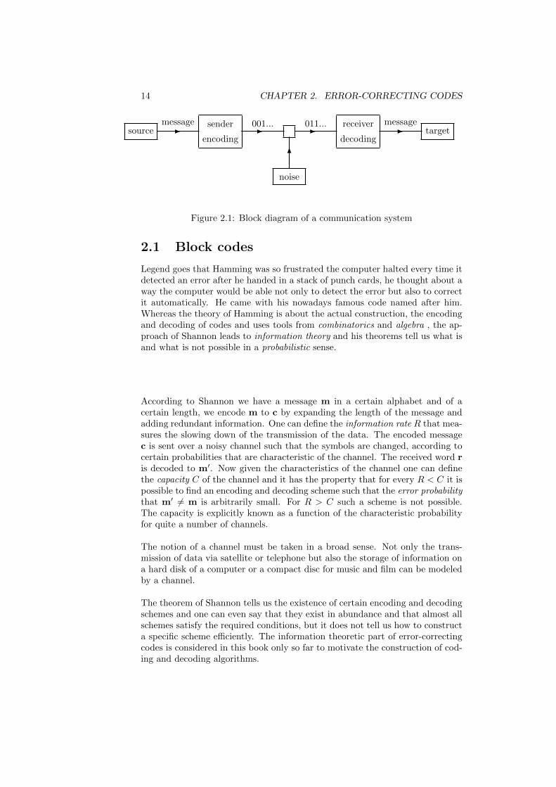
Figure 2.1: Block diagram of a communication system
2.1 Block codes
Legend goes that Hamming was so frustrated the computer halted every time itdetected an error after he handed in a stack of punch cards, he thought about away the computer would be able not only to detect the error but also to correctit automatically. He came with his nowadays famous code named after him.Whereas the theory of Hamming is about the actual construction, the encodingand decoding of codes and uses tools from combinatorics and algebra , the ap-proach of Shannon leads to information theory and his theorems tell us what isand what is not possible in a probabilistic sense.
According to Shannon we have a message m in a certain alphabet and of acertain length, we encode m to c by expanding the length of the message andadding redundant information. One can define the information rate R that mea-sures the slowing down of the transmission of the data. The encoded messagec is sent over a noisy channel such that the symbols are changed, according tocertain probabilities that are characteristic of the channel. The received word ris decoded to m′. Now given the characteristics of the channel one can definethe capacity C of the channel and it has the property that for every R < C it ispossible to find an encoding and decoding scheme such that the error probabilitythat m′ 6= m is arbitrarily small. For R > C such a scheme is not possible.The capacity is explicitly known as a function of the characteristic probabilityfor quite a number of channels.
The notion of a channel must be taken in a broad sense. Not only the trans-mission of data via satellite or telephone but also the storage of information ona hard disk of a computer or a compact disc for music and film can be modeledby a channel.
The theorem of Shannon tells us the existence of certain encoding and decodingschemes and one can even say that they exist in abundance and that almost allschemes satisfy the required conditions, but it does not tell us how to constructa specific scheme efficiently. The information theoretic part of error-correctingcodes is considered in this book only so far to motivate the construction of cod-ing and decoding algorithms.
2.1. BLOCK CODES 15
The situation for the best codes in terms of the maximal number of errors thatone can correct for a given information rate and code length is not so clear.Several existence and nonexistence theorems are known, but the exact bound isin fact still an open problem.
2.1.1 Repetition, product and Hamming codes
Adding a parity check such that the number of ones is even, is a well-knownway to detect one error. But this does not correct the error.
Example 2.1.1 Replacing every symbol by a threefold repetition gives the pos-sibility of correcting one error in every 3-tuple of symbols in a received wordby a majority vote. The price one has to pay is that the transmission is threetimes slower. We see here the two conflicting demands of error-correction: tocorrect as many errors as possible and to transmit as fast a possible. Noticefurthermore that in case two errors are introduced by transmission the majoritydecoding rule will introduce an decoding error.
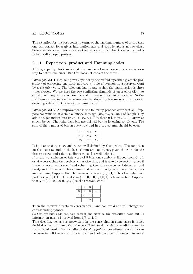
Example 2.1.2 An improvement is the following product construction. Sup-pose we want to transmit a binary message (m1,m2,m3,m4) of length 4 byadding 5 redundant bits (r1, r2, r3, r4, r5). Put these 9 bits in a 3 × 3 array asshown below. The redundant bits are defined by the following conditions. Thesum of the number of bits in every row and in every column should be even.
m1 m2 r1
m3 m4 r2
r3 r4 r5
It is clear that r1, r2, r3 and r4 are well defined by these rules. The conditionon the last row and on the last column are equivalent, given the rules for thefirst two rows and columns. Hence r5 is also well defined.If in the transmission of this word of 9 bits, one symbol is flipped from 0 to 1or vice versa, then the receiver will notice this, and is able to correct it. Since ifthe error occurred in row i and column j, then the receiver will detect an oddparity in this row and this column and an even parity in the remaining rowsand columns. Suppose that the message is m = (1, 1, 0, 1). Then the redundantpart is r = (0, 1, 1, 0, 1) and c = (1, 1, 0, 1, 0, 1, 1, 0, 1) is transmitted. Supposethat y = (1, 1, 0, 1, 0, 0, 1, 0, 1) is the received word.
1 1 00 1 0 ←1 0 1
↑
Then the receiver detects an error in row 2 and column 3 and will change thecorresponding symbol.So this product code can also correct one error as the repetition code but itsinformation rate is improved from 1/3 to 4/9.This decoding scheme is incomplete in the sense that in some cases it is notdecided what to do and the scheme will fail to determine a candidate for thetransmitted word. That is called a decoding failure. Sometimes two errors canbe corrected. If the first error is in row i and column j, and the second in row i′
16 CHAPTER 2. ERROR-CORRECTING CODES
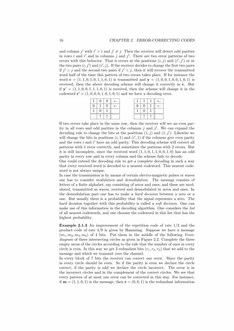
and column j′ with i′ > i and j′ 6= j. Then the receiver will detect odd paritiesin rows i and i′ and in columns j and j′. There are two error patterns of twoerrors with this behavior. That is errors at the positions (i, j) and (i′, j′) or atthe two pairs (i, j′) and (i′, j). If the receiver decides to change the first two pairsif j′ > j and the second two pairs if j′ < j, then it will recover the transmittedword half of the time this pattern of two errors takes place. If for instance theword c = (1, 1, 0, 1, 0, 1, 1, 0, 1) is transmitted and y = (1, 0, 0, 1, 0, 0, 1, 0, 1) isreceived, then the above decoding scheme will change it correctly in c. Butif y′ = (1, 1, 0, 0, 1, 1, 1, 0, 1) is received, then the scheme will change it in thecodeword c′ = (1, 0, 0, 0, 1, 0, 1, 0, 1) and we have a decoding error.
1 0 0 ←0 1 0 ←1 0 1
↑ ↑
1 1 1 ←0 0 1 ←1 0 1
↑ ↑
If two errors take place in the same row, then the receiver will see an even par-ity in all rows and odd parities in the columns j and j′. We can expand thedecoding rule to change the bits at the positions (1, j) and (1, j′). Likewise wewill change the bits in positions (i, 1) and (i′, 1) if the columns give even parityand the rows i and i′ have an odd parity. This decoding scheme will correct allpatterns with 1 error correctly, and sometimes the patterns with 2 errors. Butit is still incomplete, since the received word (1, 1, 0, 1, 1, 0, 0, 1, 0) has an oddparity in every row and in every column and the scheme fails to decode.One could extend the decoding rule to get a complete decoding in such a waythat every received word is decoded to a nearest codeword. This nearest code-word is not always unique.In case the transmission is by means of certain electro-magnetic pulses or wavesone has to consider modulation and demodulation. The message consists ofletters of a finite alphabet, say consisting of zeros and ones, and these are mod-ulated, transmitted as waves, received and demodulated in zeros and ones. Inthe demodulation part one has to make a hard decision between a zero or aone. But usually there is a probability that the signal represents a zero. Thehard decision together with this probability is called a soft decision. One canmake use of this information in the decoding algorithm. One considers the listof all nearest codewords, and one chooses the codeword in this list that has thehighest probability.
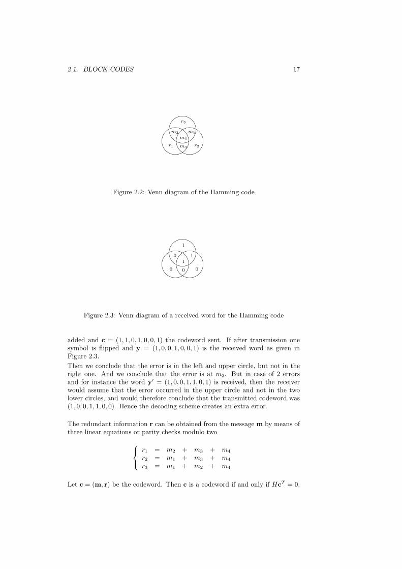
Example 2.1.3 An improvement of the repetition code of rate 1/3 and theproduct code of rate 4/9 is given by Hamming. Suppose we have a message(m1,m2,m3,m4) of 4 bits. Put them in the middle of the following Venn-diagram of three intersecting circles as given in Figure 2.2. Complete the threeempty areas of the circles according to the rule that the number of ones in everycircle is even. In this way we get 3 redundant bits (r1, r2, r3) that we add to themessage and which we transmit over the channel.In every block of 7 bits the receiver can correct one error. Since the parityin every circle should be even. So if the parity is even we declare the circlecorrect, if the parity is odd we declare the circle incorrect. The error is inthe incorrect circles and in the complement of the correct circles. We see thatevery pattern of at most one error can be corrected in this way. For instance,if m = (1, 1, 0, 1) is the message, then r = (0, 0, 1) is the redundant information
2.1. BLOCK CODES 17
&%'$&%'$&%'$r1 r2
r3
m4
m3
m2 m1
Figure 2.2: Venn diagram of the Hamming code
&%'$&%'$&%'$0 0
1
1
0
0 1
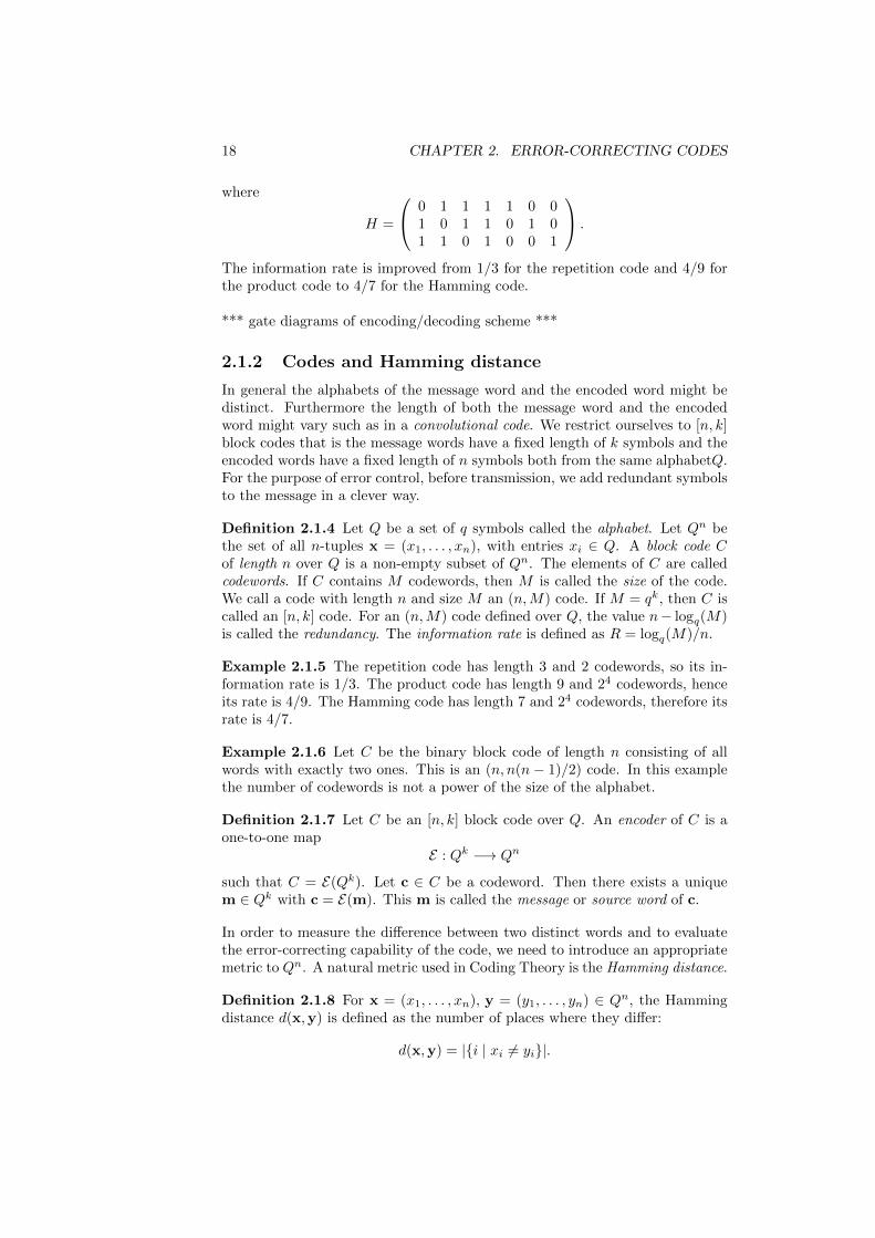
Figure 2.3: Venn diagram of a received word for the Hamming code
added and c = (1, 1, 0, 1, 0, 0, 1) the codeword sent. If after transmission onesymbol is flipped and y = (1, 0, 0, 1, 0, 0, 1) is the received word as given inFigure 2.3.
Then we conclude that the error is in the left and upper circle, but not in theright one. And we conclude that the error is at m2. But in case of 2 errorsand for instance the word y′ = (1, 0, 0, 1, 1, 0, 1) is received, then the receiverwould assume that the error occurred in the upper circle and not in the twolower circles, and would therefore conclude that the transmitted codeword was(1, 0, 0, 1, 1, 0, 0). Hence the decoding scheme creates an extra error.
The redundant information r can be obtained from the message m by means ofthree linear equations or parity checks modulo two r1 = m2 + m3 + m4
r2 = m1 + m3 + m4
r3 = m1 + m2 + m4
Let c = (m, r) be the codeword. Then c is a codeword if and only if HcT = 0,
18 CHAPTER 2. ERROR-CORRECTING CODES
where
H =
0 1 1 1 1 0 01 0 1 1 0 1 01 1 0 1 0 0 1
.
The information rate is improved from 1/3 for the repetition code and 4/9 forthe product code to 4/7 for the Hamming code.
*** gate diagrams of encoding/decoding scheme ***
2.1.2 Codes and Hamming distance
In general the alphabets of the message word and the encoded word might bedistinct. Furthermore the length of both the message word and the encodedword might vary such as in a convolutional code. We restrict ourselves to [n, k]block codes that is the message words have a fixed length of k symbols and theencoded words have a fixed length of n symbols both from the same alphabetQ.For the purpose of error control, before transmission, we add redundant symbolsto the message in a clever way.
Definition 2.1.4 Let Q be a set of q symbols called the alphabet. Let Qn bethe set of all n-tuples x = (x1, . . . , xn), with entries xi ∈ Q. A block code Cof length n over Q is a non-empty subset of Qn. The elements of C are calledcodewords. If C contains M codewords, then M is called the size of the code.We call a code with length n and size M an (n,M) code. If M = qk, then C iscalled an [n, k] code. For an (n,M) code defined over Q, the value n− logq(M)is called the redundancy. The information rate is defined as R = logq(M)/n.
Example 2.1.5 The repetition code has length 3 and 2 codewords, so its in-formation rate is 1/3. The product code has length 9 and 24 codewords, henceits rate is 4/9. The Hamming code has length 7 and 24 codewords, therefore itsrate is 4/7.
Example 2.1.6 Let C be the binary block code of length n consisting of allwords with exactly two ones. This is an (n, n(n − 1)/2) code. In this examplethe number of codewords is not a power of the size of the alphabet.
Definition 2.1.7 Let C be an [n, k] block code over Q. An encoder of C is aone-to-one map
E : Qk −→ Qn
such that C = E(Qk). Let c ∈ C be a codeword. Then there exists a uniquem ∈ Qk with c = E(m). This m is called the message or source word of c.
In order to measure the difference between two distinct words and to evaluatethe error-correcting capability of the code, we need to introduce an appropriatemetric to Qn. A natural metric used in Coding Theory is the Hamming distance.
Definition 2.1.8 For x = (x1, . . . , xn), y = (y1, . . . , yn) ∈ Qn, the Hammingdistance d(x,y) is defined as the number of places where they differ:
d(x,y) = |i | xi 6= yi|.
2.1. BLOCK CODES 19
x
d(x,y)
HHHHHHj
y
HHHH
HHY d(y,z)
: z9
d(x,z)
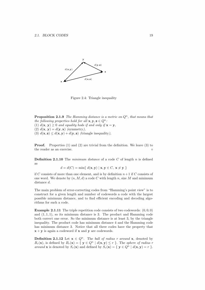
Figure 2.4: Triangle inequality
Proposition 2.1.9 The Hamming distance is a metric on Qn, that means thatthe following properties hold for all x,y, z ∈ Qn:(1) d(x, y) ≥ 0 and equality hods if and only if x = y,(2) d(x, y) = d(y,x) (symmetry),(3) d(x, z) ≤ d(x,y) + d(y, z) (triangle inequality),
Proof. Properties (1) and (2) are trivial from the definition. We leave (3) tothe reader as an exercise.
Definition 2.1.10 The minimum distance of a code C of length n is definedas
d = d(C) = min d(x,y) | x,y ∈ C, x 6= y
if C consists of more than one element, and is by definition n+1 if C consists ofone word. We denote by (n,M, d) a code C with length n, size M and minimumdistance d.
The main problem of error-correcting codes from “Hamming’s point view” is toconstruct for a given length and number of codewords a code with the largestpossible minimum distance, and to find efficient encoding and decoding algo-rithms for such a code.
Example 2.1.11 The triple repetition code consists of two codewords: (0, 0, 0)and (1, 1, 1), so its minimum distance is 3. The product and Hamming codeboth correct one error. So the minimum distance is at least 3, by the triangleinequality. The product code has minimum distance 4 and the Hamming codehas minimum distance 3. Notice that all three codes have the property thatx + y is again a codeword if x and y are codewords.
Definition 2.1.12 Let x ∈ Qn. The ball of radius r around x, denoted byBr(x), is defined by Br(x) = y ∈ Qn | d(x,y) ≤ r . The sphere of radius raround x is denoted by Sr(x) and defined by Sr(x) = y ∈ Qn | d(x,y) = r .
20 CHAPTER 2. ERROR-CORRECTING CODES
&%'$
*
q q q q q q qq q q q q q qq q q q q q qq q q q q q qq q q q q q qq q q q q q qq q q q q q q
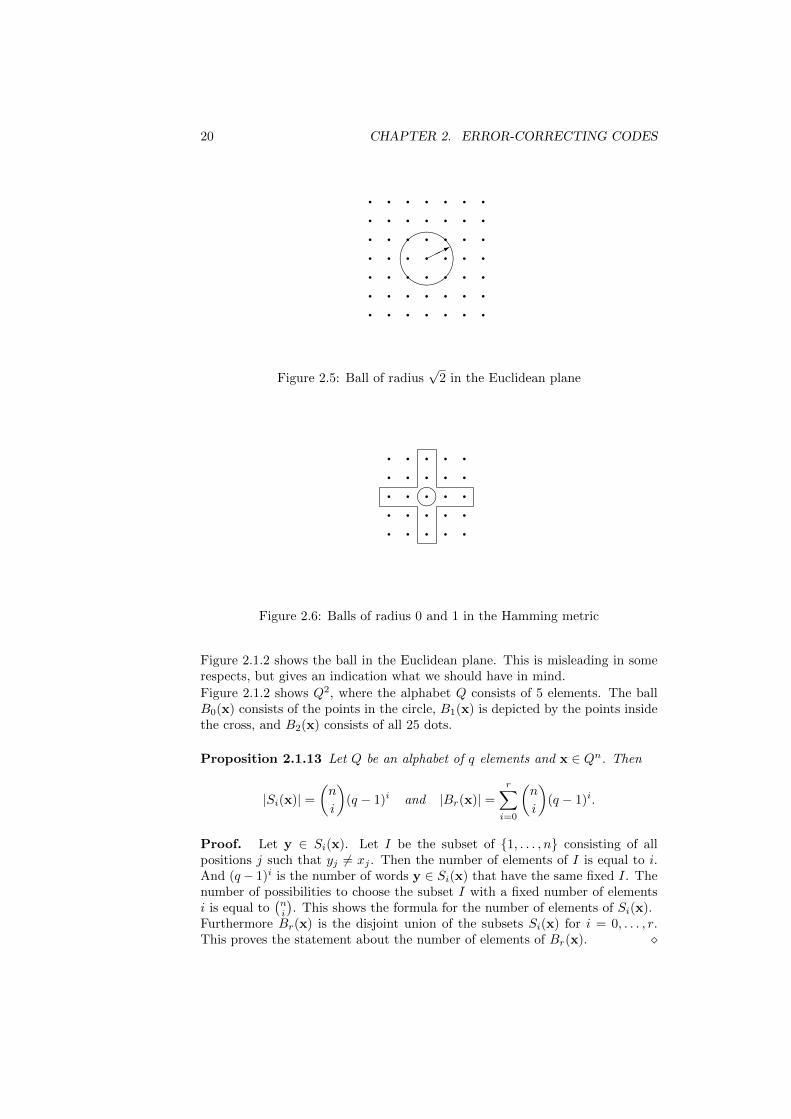
Figure 2.5: Ball of radius√
2 in the Euclidean plane
mq q q q qq q q q qq q q q qq q q q qq q q q q
Figure 2.6: Balls of radius 0 and 1 in the Hamming metric
Figure 2.1.2 shows the ball in the Euclidean plane. This is misleading in somerespects, but gives an indication what we should have in mind.
Figure 2.1.2 shows Q2, where the alphabet Q consists of 5 elements. The ballB0(x) consists of the points in the circle, B1(x) is depicted by the points insidethe cross, and B2(x) consists of all 25 dots.
Proposition 2.1.13 Let Q be an alphabet of q elements and x ∈ Qn. Then
|Si(x)| =(n
i
)(q − 1)i and |Br(x)| =
r∑i=0
(n
i
)(q − 1)i.
Proof. Let y ∈ Si(x). Let I be the subset of 1, . . . , n consisting of allpositions j such that yj 6= xj . Then the number of elements of I is equal to i.And (q− 1)i is the number of words y ∈ Si(x) that have the same fixed I. Thenumber of possibilities to choose the subset I with a fixed number of elementsi is equal to
(ni
). This shows the formula for the number of elements of Si(x).
Furthermore Br(x) is the disjoint union of the subsets Si(x) for i = 0, . . . , r.This proves the statement about the number of elements of Br(x).
2.2. LINEAR CODES 21
2.1.3 Exercises
2.1.1 Consider the code of length 8 that is obtained by deleting the last entryr5 from the product code of Example 2.1.2. Show that this code corrects oneerror.
2.1.2 Give a gate diagram of the decoding algorithm for the product code ofExample 2.1.2 that corrects always 1 error and sometimes 2 errors.
2.1.3 Give a proof of Proposition 2.1.9 (3), that is the triangle inequality ofthe Hamming distance.
2.1.4 Let Q be an alphabet of q elements. Let x,y ∈ Qn have distance d.Show that the number of elements in the intersection Br(x)∩Bs(y) is equal to∑
i,j,k
(d
i
)(d− ij
)(n− dk
)(q − 2)j(q − 1)k,
where i, j and k are non-negative integers such that i + j ≤ d, k ≤ n − d,i+ j + k ≤ r and d− i+ k ≤ s.
2.1.5 Write a procedure in GAP that takes n as an input and constructs thecode as in Example 2.1.6.
2.2 Linear Codes
Linear codes are introduced in case the alphabet is a finite field. These codeshave more structure and are therefore more tangible than arbitrary codes.
2.2.1 Linear codes
If the alphabet Q is a finite field, then Qn is a vector space. This is for instancethe case if Q = 0, 1 = F2. Therefore it is natural to look at codes in Qn thathave more structure, in particular that are linear subspaces.
Definition 2.2.1 A linear code C is a linear subspace of Fnq , where Fq stands forthe finite field with q elements. The dimension of a linear code is its dimensionas a linear space over Fq. We denote a linear code C over Fq of length n anddimension k by [n, k]q, or simply by [n, k]. If furthermore the minimum distanceof the code is d, then we call by [n, k, d]q or [n, k, d] the parameters of the code.
It is clear that for a linear [n, k] code over Fq, its size M = qk. The informationrate is R = k/n and the redundancy is n− k.
Definition 2.2.2 For a word x ∈ Fnq , its support, denoted by supp(x), is definedas the set of nonzero coordinate positions, so supp(x) = i | xi 6= 0. The weightof x is defined as the number of elements of its support, which is denoted bywt(x). The minimum weight of a code C, denoted by mwt(C), is defined as theminimal value of the weights of the nonzero codewords:
mwt(C) = min wt(c) | c ∈ C, c 6= 0 ,
in case there is a c ∈ C not equal to 0, and n+ 1 otherwise.
22 CHAPTER 2. ERROR-CORRECTING CODES
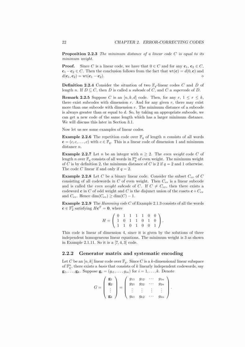
Proposition 2.2.3 The minimum distance of a linear code C is equal to itsminimum weight.
Proof. Since C is a linear code, we have that 0 ∈ C and for any c1, c2 ∈ C,c1−c2 ∈ C. Then the conclusion follows from the fact that wt(c) = d(0, c) andd(c1, c2) = wt(c1 − c2).
Definition 2.2.4 Consider the situation of two Fq-linear codes C and D oflength n. If D ⊆ C, then D is called a subcode of C, and C a supercode of D.
Remark 2.2.5 Suppose C is an [n, k, d] code. Then, for any r, 1 ≤ r ≤ k,there exist subcodes with dimension r. And for any given r, there may existmore than one subcode with dimension r. The minimum distance of a subcodeis always greater than or equal to d. So, by taking an appropriate subcode, wecan get a new code of the same length which has a larger minimum distance.We will discuss this later in Section 3.1.
Now let us see some examples of linear codes.
Example 2.2.6 The repetition code over Fq of length n consists of all wordsc = (c, c, . . . , c) with c ∈ Fq. This is a linear code of dimension 1 and minimumdistance n.
Example 2.2.7 Let n be an integer with n ≥ 2. The even weight code C oflength n over Fq consists of all words in Fnq of even weight. The minimum weightof C is by definition 2, the minimum distance of C is 2 if q = 2 and 1 otherwise.The code C linear if and only if q = 2.
Example 2.2.8 Let C be a binary linear code. Consider the subset Cev of Cconsisting of all codewords in C of even weight. Then Cev is a linear subcodeand is called the even weight subcode of C. If C 6= Cev, then there exists acodeword c in C of odd weight and C is the disjunct union of the cosets c+Cevand Cev. Hence dim(Cev) ≥ dim(C)− 1.
Example 2.2.9 The Hamming code C of Example 2.1.3 consists of all the wordsc ∈ F7
2 satisfying HcT = 0, where
H =
0 1 1 1 1 0 01 0 1 1 0 1 01 1 0 1 0 0 1
.
This code is linear of dimension 4, since it is given by the solutions of threeindependent homogeneous linear equations. The minimum weight is 3 as shownin Example 2.1.11. So it is a [7, 4, 3] code.
2.2.2 Generator matrix and systematic encoding
Let C be an [n, k] linear code over Fq. Since C is a k-dimensional linear subspaceof Fnq , there exists a basis that consists of k linearly independent codewords, sayg1, . . . ,gk. Suppose gi = (gi1, . . . , gin) for i = 1, . . . , k. Denote
G =
g1
g2
...gk
=
g11 g12 · · · g1n
g21 g22 · · · g2n
......
......
gk1 gk2 · · · gkn
.
2.2. LINEAR CODES 23
Every codeword c can be written uniquely as a linear combination of thebasis elements, so c = m1g1 + · · · + mkgk where m1, . . . ,mk ∈ Fq. Letm = (m1, . . . ,mk) ∈ Fkq . Then c = mG. The encoding
E : Fkq −→ Fnq ,
from the message word m ∈ Fkq to the codeword c ∈ Fnq can be done efficientlyby a matrix multiplication.
c = E(m) := mG.
Definition 2.2.10 A k × n matrix G with entries in Fq is called a generatormatrix of an Fq-linear code C if the rows of G are a basis of C.
A given [n, k] code C can have more than one generator matrix, however everygenerator matrix of C is a k×n matrix of rank k. Conversely every k×n matrixof rank k is the generator matrix of an Fq-linear [n, k] code.
Example 2.2.11 The linear codes with parameters [n, 0, n+1] and [n, n, 1] arethe trivial codes 0 and Fnq , and they have the empty matrix and the n × nidentity matrix In as generator matrix, respectively.
Example 2.2.12 The repetition code of length n has generator matrix
G = ( 1 1 · · · 1 ).
Example 2.2.13 The binary even-weight code of length n has for instance thefollowing two generator matrices
1 1 0 . . . 0 0 00 1 1 . . . 0 0 0...
......
. . ....
......
0 0 0 . . . 1 1 00 0 0 . . . 0 1 1
and
1 0 . . . 0 0 10 1 . . . 0 0 1...
.... . .
......
...0 0 . . . 1 0 10 0 . . . 0 1 1
.
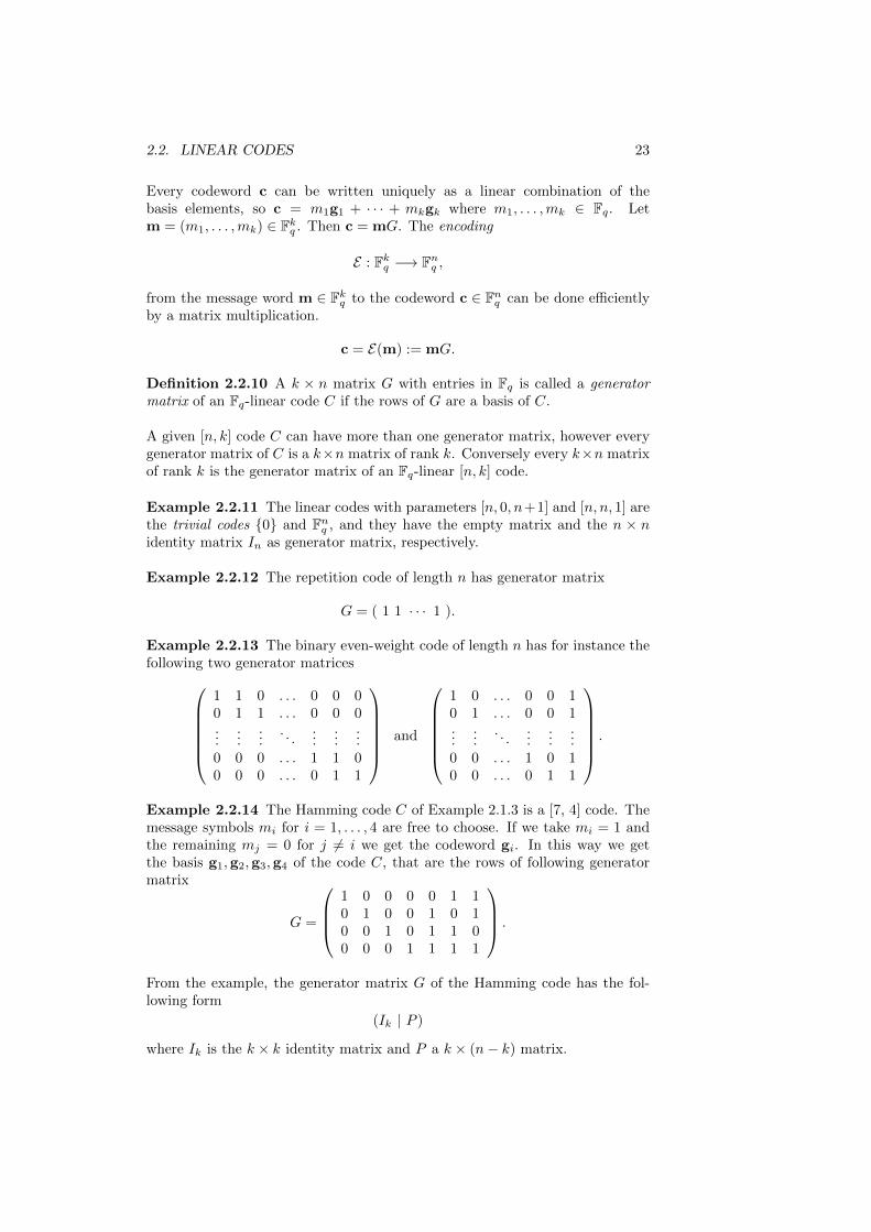
Example 2.2.14 The Hamming code C of Example 2.1.3 is a [7, 4] code. Themessage symbols mi for i = 1, . . . , 4 are free to choose. If we take mi = 1 andthe remaining mj = 0 for j 6= i we get the codeword gi. In this way we getthe basis g1,g2,g3,g4 of the code C, that are the rows of following generatormatrix
G =
1 0 0 0 0 1 10 1 0 0 1 0 10 0 1 0 1 1 00 0 0 1 1 1 1
.
From the example, the generator matrix G of the Hamming code has the fol-lowing form
(Ik | P )
where Ik is the k × k identity matrix and P a k × (n− k) matrix.
24 CHAPTER 2. ERROR-CORRECTING CODES
Remark 2.2.15 Let G be a generator matrix of C. From Linear Algebra, seeSection ??, we know that we can transform G by Gaussian elimination in arow equivalent matrix in row reduced echelon form by a sequence of the threeelementary row operations:1) interchanging two rows,2) multiplying a row with a nonzero constant,3) adding one row to another row.Moreover for a given matrix G, there is exactly one row equivalent matrix thatis in row reduced echelon form, denoted by rref(G). In the following propositionit is stated that rref(G) is also a generator matrix of C.
Proposition 2.2.16 Let G be a generator matrix of C. Then rref(G) is alsoa generator matrix of C and rref(G) = MG, where M is an invertible k × kmatrix with entries in Fq.
Proof. The row reduced echelon form rref(G) of G is obtained from G by asequence of elementary operations. The code C is equal to the row space of G,and the row space does not change under elementary row operations. So rref(G)generates the same code C.Furthermore rref(G) = E1 · · ·ElG, where E1, . . . , El are the elementary matricesthat correspond to the elementary row operations. Let M = E1 · · ·El. Then Mis an invertible matrix, since the Ei are invertible, and rref(G) = MG.
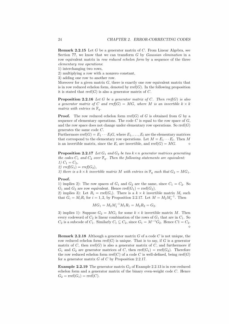
Proposition 2.2.17 Let G1 and G2 be two k×n generator matrices generatingthe codes C1 and C2 over Fq. Then the following statements are equivalent:1) C1 = C2,2) rref(G1) = rref(G2),3) there is a k× k invertible matrix M with entries in Fq such that G2 = MG1.
Proof.1) implies 2): The row spaces of G1 and G2 are the same, since C1 = C2. SoG1 and G2 are row equivalent. Hence rref(G1) = rref(G2).2) implies 3): Let Ri = rref(Gi). There is a k × k invertible matrix Mi suchthat Gi = MiRi for i = 1, 2, by Proposition 2.2.17. Let M = M2M
−11 . Then
MG1 = M2M−11 M1R1 = M2R2 = G2.
3) implies 1): Suppose G2 = MG1 for some k × k invertible matrix M . Thenevery codeword of C2 is linear combination of the rows of G1 that are in C1. SoC2 is a subcode of C1. Similarly C1 ⊆ C2, since G1 = M−1G2. Hence C1 = C2.
Remark 2.2.18 Although a generator matrix G of a code C is not unique, therow reduced echelon form rref(G) is unique. That is to say, if G is a generatormatrix of C, then rref(G) is also a generator matrix of C, and furthermore ifG1 and G2 are generator matrices of C, then rref(G1) = rref(G2). Thereforethe row reduced echelon form rref(C) of a code C is well-defined, being rref(G)for a generator matrix G of C by Proposition 2.2.17.
Example 2.2.19 The generator matrix G2 of Example 2.2.13 is in row-reducedechelon form and a generator matrix of the binary even-weight code C. HenceG2 = rref(G1) = rref(C).
2.2. LINEAR CODES 25
Definition 2.2.20 Let C be an [n, k] code. The code is called systematic atthe positions (j1, . . . , jk) if for all m ∈ Fkq there exists a unique codeword c suchthat cji = mi for all i = 1, . . . , k. In that case, the set j1, . . . , jk is called aninformation set. A generator matrix G of C is called systematic at the positions(j1, . . . , jk) if the k × k submatrix G′ consisting of the k columns of G at thepositions (j1, . . . , jk) is the identity matrix. For such a matrix G the mappingm 7→mG is called systematic encoding.
Remark 2.2.21 If a generator matrix G of C is systematic at the positions(j1, . . . , jk) and c is a codeword, then c = mG for a unique m ∈ Fkq andcji = mi for all i = 1, . . . , k. Hence C is systematic at the positions (j1, . . . , jk).Now suppose that the ji with 1 ≤ j1 < · · · < jk ≤ n indicate the positions ofthe pivots of rref(G). Then the code C and the generator matrix rref(G) aresystematic at the positions (j1, . . . , jk).
Proposition 2.2.22 Let C be a code with generator matrix G. Then C issystematic at the positions j1, . . . , jk if and only if the k columns of G at thepositions j1, . . . , jk are linearly independent.
Proof. Let G be a generator matrix of C. Let G′ be the k × k submatrixof G consisting of the k columns at the positions (j1, . . . , jk). Suppose C issystematic at the positions (j1, . . . , jk). Then the map given by x 7→ xG′ isinjective. Hence the columns of G′ are linearly independent.Conversely, if the columns of G′ are linearly independent, then there exists ak × k invertible matrix M such that MG′ is the identity matrix. Hence MG isa generator matrix of C and C is systematic at (j1, . . . , jk).
Example 2.2.23 Consider a code C with generator matrix
G =
1 0 1 0 1 0 1 01 1 0 0 1 1 0 01 1 0 1 0 0 1 01 1 0 1 0 0 1 1
.
Then
rref(C) = rref(G) =
1 0 1 0 1 0 1 00 1 1 0 0 1 1 00 0 0 1 1 1 1 00 0 0 0 0 0 0 1
and the code is systematic at the positions 1, 2, 4 and 8. By the way we noticethat the minimum distance of the code is 1.
2.2.3 Exercises
2.2.1 Determine for the product code of Example 2.1.2 the number of code-words, the number of codewords of a given weight, the minimum weight andthe minimum distance. Express the redundant bits rj for j = 1, . . . , 5 as linearequations over F2 in the message bits mi for i = 1, . . . , 4. Give a 5×9 matrix Hsuch that c = (m, r) is a codeword of the product code if and only if HcT = 0,where m is the message of 4 bits mi and r is the vector with the 5 redundantbits rj .
26 CHAPTER 2. ERROR-CORRECTING CODES
2.2.2 Let x and y be binary words of the same length. Show that
wt(x + y) = wt(x) + wt(y)− 2|supp(x) ∩ supp(y)|.
2.2.3 Let C be an Fq-linear code with generator matrix G. Let q = 2. Showthat every codeword of C has even weight if and only if every row of a G haseven weight. Show by means of a counter example that the above statement isnot true if q 6= 2.
2.2.4 Consider the following matrix with entries in F5
G =
1 1 1 1 1 00 1 2 3 4 00 1 4 4 1 1
.
Show that G is a generator matrix of a [5, 3, 3] code. Give the row reducedechelon form of this code.
2.2.5 Compute the complexity of the encoding of a linear [n, k] code by anarbitrary generator matrix G and in case G is systematic, respectively, in termsof the number of additions and multiplications.
2.3 Parity checks and dual code
Linear codes are implicitly defined by parity check equations and the dual of acode is introduced.
2.3.1 Parity check matrix
There are two standard ways to describe a subspace, explicitly by giving a basis,or implicitly by the solution space of a set of homogeneous linear equations.Therefore there are two ways to describe a linear code. That is explicitly as wehave seen by a generator matrix, or implicitly by a set of homogeneous linearequations that is by the null space of a matrix.
Let C be an Fq-linear [n, k] code. Suppose that H is an m × n matrix withentries in Fq. Let C be the null space of H. So C is the set of all c ∈ Fnq such
that HcT = 0. These m homogeneous linear equations are called parity checkequations, or simply parity checks. The dimension k of C is at least n −m. Ifthere are dependent rows in the matrix H, that is if k > n −m, then we candelete a few rows until we obtain an (n − k) × n matrix H ′ with independentrows and with the same null space as H. So H ′ has rank n− k.
Definition 2.3.1 An (n− k)× n matrix of rank n− k is called a parity checkmatrix of an [n, k] code C if C is the null space of this matrix.
Remark 2.3.2 The parity check matrix of a code can be used for error detec-tion. This is useful in a communication channel where one asks for retransmis-sion in case more than a certain number of errors occurred. Suppose that Cis a linear code of minimum distance d and H is a parity check matrix of C.Suppose that the codeword c is transmitted and r = c + e is received. Then e
2.3. PARITY CHECKS AND DUAL CODE 27
is called the error vector and wt(e) the number of errors. Now HrT = 0 if thereis no error and HrT 6= 0 for all e such that 0 < wt(e) < d. Therefore we candetect any pattern of t errors with t < d. But not more, since if the error vectoris equal to a nonzero codeword of minimal weight d, then the receiver wouldassume that no errors have been made. The vector HrT is called the syndromeof the received word.
We show that every linear code has a parity check matrix and we give a methodto obtain such a matrix in case we have a generator matrix G of the code.
Proposition 2.3.3 Suppose C is an [n, k] code. Let Ik be the k × k identitymatrix. Let P be a k × (n − k) matrix. Then, (Ik|P ) is a generator matrix ofC if and only if (−PT |In−k) is a parity check matrix of C.
Proof. Every codeword c is of the form mG with m ∈ Fkq . Suppose that thegenerator matrix G is systematic at the first k positions. So c = (m, r) withr ∈ Fn−kq and r = mP . Hence for a word of the form c = (m, r) with m ∈ Fkqand r ∈ Fn−kq the following statements are equivalent:
c is a codeword ,
−mP + r = 0,
−PTmT + rT = 0,(−PT |In−k
)(m, r)T = 0,(
−PT |In−k)cT = 0.
Hence(−PT |In−k
)is a parity check matrix of C. The converse is proved simi-
larly.
Example 2.3.4 The trivial codes 0 and Fnq have In and the empty matrixas parity check matrix, respectively.
Example 2.3.5 As a consequence of Proposition 2.3.3 we see that a paritycheck matrix of the binary even weight code is equal to the generator matrix( 1 1 · · · 1 ) of the repetition code, and the generator matrix G2 of the binaryeven weight code of Example 2.2.13 is a parity check matrix of the repetitioncode.
Example 2.3.6 The ISBN code of a book consists of a word (b1, . . . , b10) of 10symbols of the alphabet with the 11 elements: 0, 1, 2, . . . , 9 and X of the finitefield F11, where X is the symbol representing 10, that satisfies the parity checkequation:
b1 + 2b2 + 3b3 + · · ·+ 10b10 = 0.
Clearly his code detects one error. This code corrects many patterns of onetransposition of two consecutive symbols. Suppose that the symbols bi and bi+1
are interchanged and there are no other errors, then the parity check gives asoutcome
ibi+1 + (i+ 1)bi +∑
j 6=i,i+1
jbj = s.
28 CHAPTER 2. ERROR-CORRECTING CODES
We know that∑j jbj = 0, since (b1, . . . , b10) is an ISBN codeword. Hence
s = bi − bi+1. But this position i is in general not unique.Consider for instance the following code: 0444815933. Then the checksum gives4, so it is not a valid ISBN code. Now assume that the code is the resultof transposition of two consecutive symbols. Then 4044815933, 0448415933,0444185933, 0444851933 and 0444819533 are the possible ISBN codes. Thefirst and third code do not match with existing books. The second, fourthand fifth code correspond to books with the titles: “The revenge of the dragonlady,” “The theory of error-correcting codes” and “Nagasaki’s symposium onChernobyl,” respectively.
Example 2.3.7 The generator matrix G of the Hamming code C in Example2.2.14 is of the form (I4|P ) and in Example 2.2.9 we see that the parity checkmatrix is equal to (PT |I3).
Remark 2.3.8 Let G be a generator matrix of an [n, k] code C. Then the rowreduced echelon form G1 = rref(G) is not systematic at the first k positions butat the positions (j1, . . . , jk) with 1 ≤ j1 < · · · < jk ≤ n. After a permutation πof the n positions with corresponding n×n permutation matrix, denoted by Π,we may assume that G2 = G1Π is of the form (Ik|P ). Now G2 is a generatormatrix of the code C2 which is not necessarily equal to C. A parity check matrixH2 for C2 is given by (−PT |In−k) according to Proposition 2.3.3. A parity checkmatrix H for C is now of the form (−PT |In−k)ΠT , since Π−1 = ΠT .
This remark motivates the following definition.
Definition 2.3.9 Let I = i1, . . . , ik be an information set of the code C.Then its complement 1, . . . , n \ I is called a check set.
Example 2.3.10 Consider the code C of Example 2.2.23 with generator matrixG. The row reduced echelon form G1 = rref(G) is systematic at the positions 1,2, 4 and 8. Let π be the permutation (348765) with corresponding permutationmatrix Π. Then G2 = G1Π = (I4|P ) and H2 = (PT |I4) with
G2 =
1 0 0 0 1 1 0 10 1 0 0 1 0 1 10 0 1 0 0 1 1 10 0 0 1 0 0 0 0
, H2 =
1 1 0 0 1 0 0 01 0 1 0 0 1 0 00 1 1 0 0 0 1 01 1 1 0 0 0 0 1
Now π−1 = (356784) and
H = H2ΠT =
1 1 1 0 0 0 0 01 0 0 1 1 0 0 00 1 0 1 0 1 0 01 1 0 1 0 0 1 0
is a parity check matrix of C.
2.3.2 Hamming and simplex codes
The following proposition gives a method to determine the minimum distance ofa code in terms of the number of dependent columns of the parity check matrix.
2.3. PARITY CHECKS AND DUAL CODE 29
Proposition 2.3.11 Let H be a parity check matrix of a code C. Then theminimum distance d of C is the smallest integer d such that d columns of H arelinearly dependent.
Proof. Let h1, . . . ,hn be the columns of H. Let c be a nonzero codewordof weight w. Let supp(c) = j1, . . . , jw with 1 ≤ j1 < · · · < jw ≤ n. ThenHcT = 0, so cj1hj1 + · · · + cjwhjw = 0 with cji 6= 0 for all i = 1, . . . , w.Therefore the columns hj1 , . . . ,hjw are dependent. Conversely if hj1 , . . . ,hjware dependent, then there exist constants a1, . . . , aw, not all zero, such thata1hj1 + · · ·+ awhjw = 0. Let c be the word defined by cj = 0 if j 6= ji for all i,and cj = ai if j = ji for some i. Then HcT = 0. Hence c is a nonzero codewordof weight at most w.
Remark 2.3.12 Let H be a parity check matrix of a code C. As a consequenceof Proposition 2.3.11 we have the following special cases. The minimum distanceof code is 1 if and only if H has a zero column. An example of this is seen inExample 2.3.10. Now suppose that H has no zero column, then the minimumdistance of C is at least 2. The minimum distance is equal to 2 if and only if Hhas two columns say hj1 ,hj2 that are dependent. In the binary case that meanshj1 = hj2 . In other words the minimum distance of a binary code is at least 3 ifand only if H has no zero columns and all columns are mutually distinct. Thisis the case for the Hamming code of Example 2.2.9. For a given redundancy rthe length of a binary linear code C of minimum distance 3 is at most 2r − 1,the number of all nonzero binary columns of length r. For arbitrary Fq, thenumber of nonzero columns with entries in Fq is qr − 1. Two such columnsare dependent if and only if one is a nonzero multiple of the other. Hence thelength of an Fq-linear code code C with d(C) ≥ 3 and redundancy r is at most(qr − 1)/(q − 1).
Definition 2.3.13 Let n = (qr − 1)/(q − 1). Let Hr(q) be a r × n matrixover Fq with nonzero columns, such that no two columns are dependent. Thecode Hr(q) with Hr(q) as parity check matrix is called a q-ary Hamming code.The code with Hr(q) as generator matrix is called a q-ary simplex code and isdenoted by Sr(q).
Proposition 2.3.14 Let r ≥ 2. Then the q-ary Hamming code Hr(q) hasparameters [(qr − 1)/(q − 1), (qr − 1)/(q − 1)− r, 3].
Proof. The rank of the matrix Hr(q) is r, since the r standard basis vectorsof weight 1 are among the columns of the matrix. So indeed Hr(q) is a paritycheck matrix of a code with redundancy r. Any 2 columns are independent byconstruction. And a column of weight 2 is a linear combination of two columnsof weight 1, and such a triple of columns exists, since r ≥ 2. Hence the minimumdistance is 3 by Proposition 2.3.11.
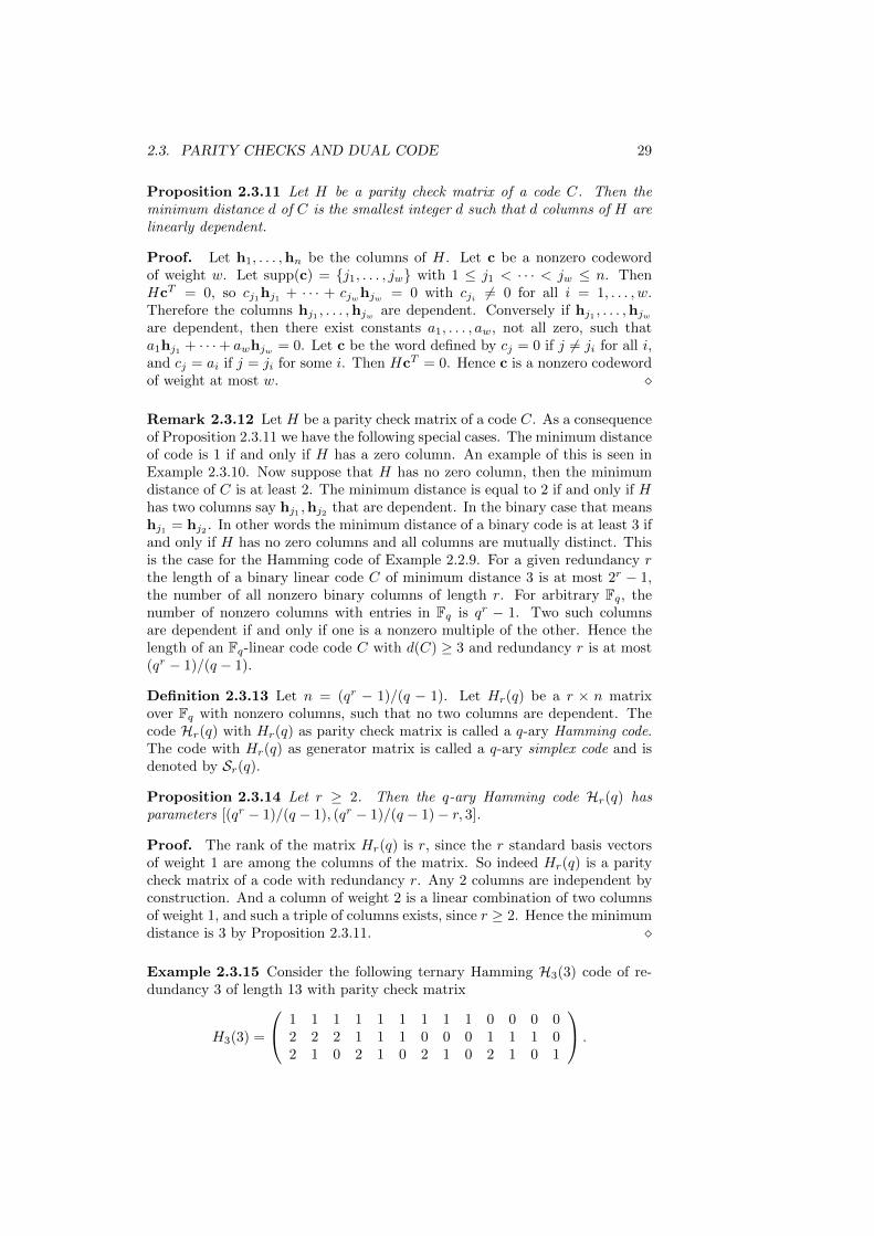
Example 2.3.15 Consider the following ternary Hamming H3(3) code of re-dundancy 3 of length 13 with parity check matrix
H3(3) =
1 1 1 1 1 1 1 1 1 0 0 0 02 2 2 1 1 1 0 0 0 1 1 1 02 1 0 2 1 0 2 1 0 2 1 0 1
.
30 CHAPTER 2. ERROR-CORRECTING CODES
By Proposition 2.3.14 the code H3(3) has parameters [13, 10, 3]. Notice thatall rows of H3(3) have weight 9. In fact every linear combination xH3(3) withx ∈ F3
3 and x 6= 0 has weight 9. So all nonzero codewords of the ternary simplexcode of dimension 3 have weight 9. Hence S3(3) is a constant weight code. Thisis a general fact of simplex codes as is stated in the following proposition.
Proposition 2.3.16 The ary simplex code Sr(q) is a constant weight code withparameters [(qr − 1)/(q − 1), r, qr−1].
Proof. We have seen already in Proposition 2.3.14 that Hr(q) has rank r, soit is indeed a generator matrix of a code of dimension r. Let c be a nonzerocodeword of the simplex code. Then c = mHr(q) for some nonzero m ∈ Frq.Let hTj be the j-th column of Hr(q). Then cj = 0 if and only if m ·hj = 0. Now
m · x = 0 is a nontrivial homogeneous linear equation. This equation has qr−1
solutions x ∈ Frq, it has qr−1 − 1 nonzero solutions. It has (qr−1 − 1)/(q − 1)
solutions x such that xT is a column of Hr(q), since for every nonzero x ∈ Frqthere is exactly one column in Hr(q) that is a nonzero multiple of xT . So thenumber of zeros of c is (qr−1 − 1)/(q− 1). Hence the weight of c is the numberof nonzeros which is qr−1.
2.3.3 Inner product and dual codes
Definition 2.3.17 The inner product on Fnq is defined by
x · y = x1y1 + · · ·+ xnyn
for x,y ∈ Fnq .
This inner product is bilinear, symmetric and nondegenerate, but the notionof “positive definite” makes no sense over a finite field as it does over the realnumbers. For instance for a binary word x ∈ Fn2 we have that x · x = 0 if andonly if the weight of x is even.
Definition 2.3.18 For an [n, k] code C we define the dualdual or orthogonalcode C⊥ as
C⊥ = x ∈ Fnq | c · x = 0 for all c ∈ C.
Proposition 2.3.19 Let C be an [n, k] code with generator matrix G. ThenC⊥ is an [n, n− k] code with parity check matrix G.
Proof. From the definition of dual codes, the following statements are equiv-alent:
x ∈ C⊥,c · x = 0 for all c ∈ C,
mGxT = 0 for all m ∈ Fkq ,
GxT = 0.
This means that C⊥ is the null space of G. Because G is a k×n matrix of rankk, the linear space C⊥ has dimension n − k and G is a parity check matrix ofC⊥.
2.3. PARITY CHECKS AND DUAL CODE 31
Example 2.3.20 The trivial codes 0 and Fnq are dual codes.
Example 2.3.21 The binary even weight code and the repetition code of thesame length are dual codes.
Example 2.3.22 The simplex code Sr(q) and the Hamming code Hr(q) aredual codes, since Hr(q) is a parity check matrix of Hr(q) and a generator matrixof Sr(q)
A subspace C of a real vector space Rn has the property that C ∩ C⊥ = 0,since the standard inner product is positive definite. Over finite fields this isnot always the case.
Definition 2.3.23 Two codes C1 and C2 in Fnq are called orthogonal if x ·y = 0
for all x ∈ C1 and y ∈ C2, and they are called dual if C2 = C⊥1 .If C ⊆ C⊥, we call C weakly self-dual or self-orthogonal. If C = C⊥, we call Cself-dual. The hull of a code C is defined by H(C) = C ∩ C⊥. A code is calledcomplementary dual if H(C) = 0.
Example 2.3.24 The binary repetition code of length n is self-orthogonal ifand only if n is even. This code is self-dual if and only if n = 2.
Proposition 2.3.25 Let C be an [n, k] code. Then:(1) (C⊥)⊥ = C.(2) C is self-dual if and only C is self-orthogonal and n = 2k.
Proof.(1) Let c ∈ C. Then c · x = 0 for all x ∈ C⊥. So C ⊆ (C⊥)⊥. Moreover,applying Proposition 2.3.19 twice, we see that C and (C⊥)⊥ have the samefinite dimension. Therefore equality holds.(2) Suppose C is self-orthogonal, then C ⊆ C⊥. Now C = C⊥ if and only ifk = n− k, by Proposition 2.3.19. So C is self-dual if and only if n = 2k.
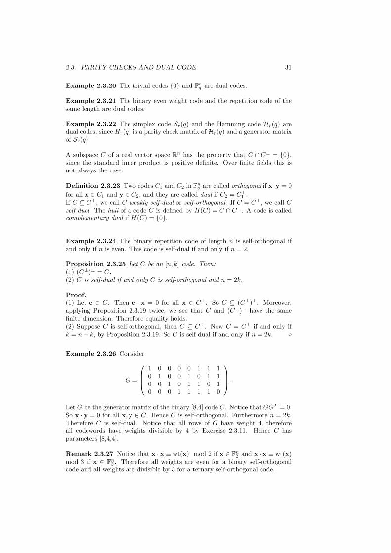
Example 2.3.26 Consider
G =
1 0 0 0 0 1 1 10 1 0 0 1 0 1 10 0 1 0 1 1 0 10 0 0 1 1 1 1 0
.
Let G be the generator matrix of the binary [8,4] code C. Notice that GGT = 0.So x · y = 0 for all x,y ∈ C. Hence C is self-orthogonal. Furthermore n = 2k.Therefore C is self-dual. Notice that all rows of G have weight 4, thereforeall codewords have weights divisible by 4 by Exercise 2.3.11. Hence C hasparameters [8,4,4].
Remark 2.3.27 Notice that x · x ≡ wt(x) mod 2 if x ∈ Fn2 and x · x ≡ wt(x)mod 3 if x ∈ Fn3 . Therefore all weights are even for a binary self-orthogonalcode and all weights are divisible by 3 for a ternary self-orthogonal code.
32 CHAPTER 2. ERROR-CORRECTING CODES
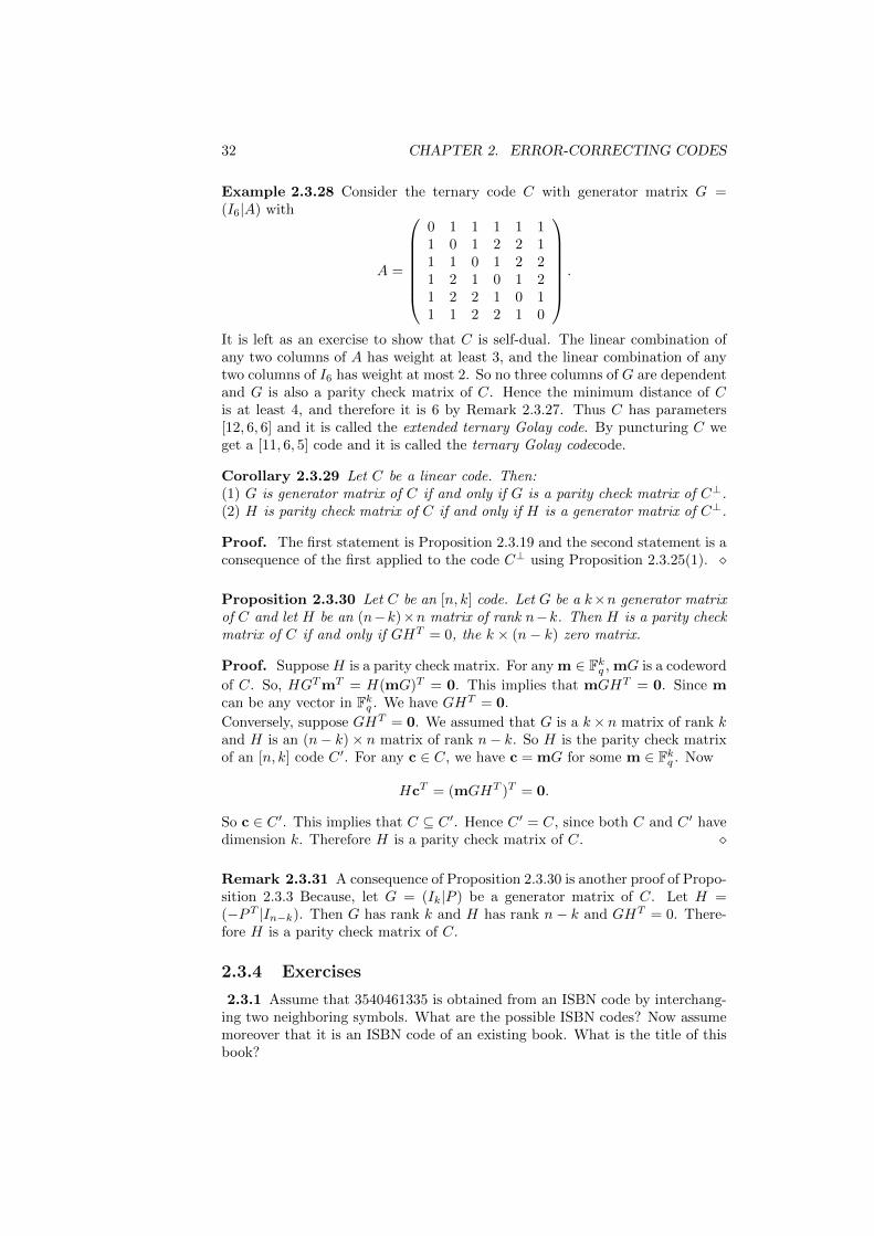
Example 2.3.28 Consider the ternary code C with generator matrix G =(I6|A) with
A =
0 1 1 1 1 11 0 1 2 2 11 1 0 1 2 21 2 1 0 1 21 2 2 1 0 11 1 2 2 1 0
.
It is left as an exercise to show that C is self-dual. The linear combination ofany two columns of A has weight at least 3, and the linear combination of anytwo columns of I6 has weight at most 2. So no three columns of G are dependentand G is also a parity check matrix of C. Hence the minimum distance of Cis at least 4, and therefore it is 6 by Remark 2.3.27. Thus C has parameters[12, 6, 6] and it is called the extended ternary Golay code. By puncturing C weget a [11, 6, 5] code and it is called the ternary Golay codecode.
Corollary 2.3.29 Let C be a linear code. Then:(1) G is generator matrix of C if and only if G is a parity check matrix of C⊥.(2) H is parity check matrix of C if and only if H is a generator matrix of C⊥.
Proof. The first statement is Proposition 2.3.19 and the second statement is aconsequence of the first applied to the code C⊥ using Proposition 2.3.25(1).
Proposition 2.3.30 Let C be an [n, k] code. Let G be a k×n generator matrixof C and let H be an (n−k)×n matrix of rank n−k. Then H is a parity checkmatrix of C if and only if GHT = 0, the k × (n− k) zero matrix.
Proof. Suppose H is a parity check matrix. For any m ∈ Fkq , mG is a codeword
of C. So, HGTmT = H(mG)T = 0. This implies that mGHT = 0. Since mcan be any vector in Fkq . We have GHT = 0.
Conversely, suppose GHT = 0. We assumed that G is a k× n matrix of rank kand H is an (n− k)× n matrix of rank n− k. So H is the parity check matrixof an [n, k] code C ′. For any c ∈ C, we have c = mG for some m ∈ Fkq . Now
HcT = (mGHT )T = 0.
So c ∈ C ′. This implies that C ⊆ C ′. Hence C ′ = C, since both C and C ′ havedimension k. Therefore H is a parity check matrix of C.
Remark 2.3.31 A consequence of Proposition 2.3.30 is another proof of Propo-sition 2.3.3 Because, let G = (Ik|P ) be a generator matrix of C. Let H =(−PT |In−k). Then G has rank k and H has rank n− k and GHT = 0. There-fore H is a parity check matrix of C.
2.3.4 Exercises
2.3.1 Assume that 3540461335 is obtained from an ISBN code by interchang-ing two neighboring symbols. What are the possible ISBN codes? Now assumemoreover that it is an ISBN code of an existing book. What is the title of thisbook?
2.4. DECODING AND THE ERROR PROBABILITY 33
2.3.2 Consider the binary product code C of Example 2.1.2. Give a paritycheck matrix and a generator matrix of this code. Determine the parameters ofthe dual of C.
2.3.3 Give a parity check matrix of the C of Exercise 2.2.4. Show that C isself-dual.
2.3.4 Consider the binary simplex code S3(2) with generator matrix H asgiven in Example 2.2.9. Show that there are exactly seven triples (i1, i2, i3) withincreasing coordinate positions such that S3(2) is not systematic at (i1, i2, i3).Give the seven four-tuples of positions that are not systematic with respect tothe Hamming code H3(2) with parity check matrix H.
2.3.5 Let C1 and C2 be linear codes of the same length. Show the followingstatements:(1) If C1 ⊆ C2, then C⊥2 ⊆ C⊥1 .(2) C1 and C2 are orthogonal if and only if C1 ⊆ C⊥2 if and only if C2 ⊆ C⊥1 .(3) (C1 ∩ C2)⊥ = C⊥1 + C⊥2 .(4) (C1 + C2)⊥ = C⊥1 ∩ C⊥2 .
2.3.6 Show that a linear code C with generator matrix G has a complementarydual if and only if det(GGT ) 6= 0.
2.3.7 Show that there exists a [2k, k] self-dual code over Fq if and only if thereis a k × k matrix P with entries in Fq such that PPT = −Ik.
2.3.8 Give an example of a ternary [4,2] self-dual code and show that there isno ternary self-dual code of length 6.
2.3.9 Show that the extended ternary Golay code in Example 2.3.28 is self-dual.
2.3.10 Show that a binary code is self-orthogonal if the weights of all code-words are divisible by 4. Hint: use Exercise 2.2.2.
2.3.11 Let C be a binary self-orthogonal code which has a generator matrixsuch that all its rows have a weight divisible by 4. Then the weights of allcodewords are divisible by 4.
2.3.12 Write a procedure either in GAP or Magma that determines whetherthe given code is self-dual or not. Test correctness of your procedure withcommands IsSelfDualCode and IsSelfDual in GAP and Magma respectively.
2.4 Decoding and the error probability
Intro
34 CHAPTER 2. ERROR-CORRECTING CODES
2.4.1 Decoding problem
Definition 2.4.1 Let C be a linear code in Fnq of minimum distance d. If cis a transmitted codeword and r is the received word, then i|ri 6= ci is theset of error positions and the number of error positions is called the number oferrors of the received word. Let e = r−c. Then e is called the error vector andr = c + e. Hence supp(e) is the set of error positions and wt(e) the number oferrors. The ei’s are called the error values.
Remark 2.4.2 If r is the received word and t′ = d(C, r) is the distance of rto the code C, then there exists a nearest codeword c′ such that t′ = d(c′, r).So there exists an error vector e′ such that r = c′ + e′ and wt(e′) = t′. If thenumber of errors t is at most (d−1)/2, then we are sure that c = c′ and e = e′.In other words, the nearest codeword to r is unique when r has distance at most(d− 1)/2 to C.
***Picture***
Definition 2.4.3 e(C) = b(d(C)− 1)/2c is called the error-correcting capacitydecoding radius of the code C.
Definition 2.4.4 A decoder D for the code C is a map
D : Fnq −→ Fnq ∪ ∗
such that D(c) = c for all c ∈ C.If E : Fkq → Fnq is an encoder of C and D : Fnq → Fkq ∪ ∗ is a map such that
D(E(m)) = m for all m ∈ Fkq , then D is called a decoder with respect to theencoder E .
Remark 2.4.5 If E is an encoder of C and D is a decoder with respect to E ,then the composition E D is a decoder of C. It is allowed that the decodergives as outcome the symbol ∗ in case it fails to find a codeword. This is calleda decoding failure. If c is the codeword sent and r is the received word andD(r) = c′ 6= c, then this is called a decoding error. If D(r) = c, then r isdecoded correctly. Notice that a decoding failure is noted on the receiving end,whereas there is no way that the decoder can detect a decoding error.
Definition 2.4.6 A complete decoder is a decoder that always gives a codewordin C as outcome. A nearest neighbor decoder, also called a minimum distancedecoder, is a complete decoder with the property thatD(r) is a nearest codeword.A decoder D for a code C is called a t-bounded distance decoder or a decoderthat corrects t errors if D(r) is a nearest codeword for all received words rwith d(C, r) ≤ t errors. A decoder for a code C with error-correcting capacitye(C) decodes up to half the minimum distance if it is an e(C)-bounded distancedecoder, where e(C) = b(d(C)− 1)/2c is the error-correcting capacity of C.
Remark 2.4.7 If D is a t-bounded distance decoder, then it is not requiredthat D gives a decoding failure as outcome for a received word r if the distanceof r to the code is strictly larger than t. In other words: D is also a t′-boundeddistance decoder for all t′ ≤ t.A nearest neighbor decoder is a t-bounded distance decoder for all t ≤ ρ(C),where ρ(C) is the covering radius of the code. A ρ(C)-bounded distance decoderis a nearest neighbor decoder, since d(C, r) ≤ ρ(C) for all received words r.
2.4. DECODING AND THE ERROR PROBABILITY 35
Definition 2.4.8 Let r be a received word with respect to a code C. A cosetleader of r + C is a choice of an element of minimal weight in the coset r + C.The weight of a coset is the minimal weight of an element in the coset. Let αibe the number of cosets of C that are of weight i. Then αC(X,Y ), the cosetleader weight enumerator of C is the polynomial defined by
αC(X,Y ) =
n∑i=0
αiXn−iY i.
Remark 2.4.9 The choice of a coset leader of the coset r + C is unique ifd(C, r) ≤ (d − 1)/2, and αi =
(ni
)(q − 1)i for all i ≤ (d − 1)/2, where d is the
minimum distance of C. Let ρ(C) be the covering radius of the code, then thereis at least one codeword c such that d(c, r) ≤ ρ(C). Hence the weight of a cosetleader is at most ρ(C) and αi = 0 for i > ρ(C). Therefore the coset leaderweight enumerator of a perfect code C of minimum distance d = 2t+ 1 is givenby
αC(X,Y ) =
t∑i=0
(n
i
)(q − 1)iXn−iY i.
The computation of the coset leader weight enumerator of a code is in generala very hard problem.
Definition 2.4.10 Let r be a received word. Let e be the chosen coset leaderof the coset r + C. The coset leader decoder gives r− e as output.
Remark 2.4.11 The coset leader decoder is a nearest neighbor decoder.
Definition 2.4.12 Let r be a received word with respect to a code C of di-mension k. Choose an (n− k)× n parity check matrix H of the code C. Thens = rHT ∈ Fn−kq is called the syndrome of r with respect to H.
Remark 2.4.13 Let C be a code of dimension k. Let r be a received word.Then r + C is called the coset of r. Now the cosets of the received words r1
and r2 are the same if and only if r1HT = r2H
T . Therefore there is a one toone correspondence between cosets of C and values of syndromes. Furthermoreevery element of Fn−kq is the syndrome of some received word r, since H has
rank n− k. Hence the number of cosets is qn−k.
A list decoder gives as output the collection of all nearest codewords.
Knowing the existence of a decoder is nice to know from a theoretical point ofview, in practice the problem is to find an efficient algorithm that computes theoutcome of the decoder. To compute of a given vector in Euclidean n-space theclosest vector to a given linear subspace can be done efficiently by an orthogonalprojection to the subspace. The corresponding problem for linear codes is ingeneral not such an easy task. This is treated in Section 6.2.1.
2.4.2 Symmetric channel
....
36 CHAPTER 2. ERROR-CORRECTING CODES
Definition 2.4.14 The q-ary symmetric channel (qSC) is a channel where q-ary words are sent with independent errors with the same cross-over probabilityp at each coordinate, with 0 ≤ p ≤ 1
2 , such that all the q − 1 wrong symbolsoccur with the same probability p/(q− 1). So a symbol is transmitted correctlywith probability 1 − p. The special case q = 2 is called the binary symmetricchannel (BSC).
picture
Remark 2.4.15 Let P (x) be the probability that the codeword x is sent. Thenthis probability is assumed to be the same for all codewords. Hence P (c) = 1
|C|for all c ∈ C. Let P (r|c) be the probability that r is received given that c issent. Then
P (r|c) =
(p
q − 1
)d(c,r)
(1− p)n−d(c,r)
for a q-ary symmetric channel.
Definition 2.4.16 For every decoding scheme and channel one defines threeprobabilities Pcd(p), Pde(p) and Pdf (p), that is the probability of correct decoding,decoding error and decoding failure, respectively. Then
Pcd(p) + Pde(p) + Pdf (p) = 1 for all 0 ≤ p ≤ 1
2.
So it suffices to find formulas for two of these three probabilities. The errorprobability, also called the error rate is defined by Perr(p) = 1− Pcd(p). Hence
Perr(p) = Pde(p) + Pdf (p).
Proposition 2.4.17 The probability of correct decoding of a decoder that cor-rects up to t errors with 2t + 1 ≤ d of a code C of minimum distance d on aq-ary symmetric channel with cross-over probability p is given by
Pcd(p) =
t∑w=0
(n
w
)pw(1− p)n−w.
Proof. Every codeword has the same probability of transmission. So
Pcd(p) =∑c∈C
P (c)∑
d(c,r)≤t
P (y|r) =1
|C|∑c∈C
∑d(c,r)≤t
P (r|c),
Now P (r|c) depends only on the distance between r and c by Remark 2.4.15.So without loss of generality we may assume that 0 is the codeword sent. Hence
Pcd(p) =∑
d(0,r)≤t
P (r|0) =
t∑w=0
(n
w
)(q − 1)w
(p
q − 1
)w(1− p)n−w
by Proposition 2.1.13. Clearing the factor (q − 1)w in the numerator and thedenominator gives the desired result. In Proposition 4.2.6 a formula will be derived for the probability of decodingerror for a decoding algorithm that corrects errors up to half the minimumdistance.
2.4. DECODING AND THE ERROR PROBABILITY 37
Example 2.4.18 Consider the binary triple repetition code. Assume that(0, 0, 0) is transmitted. In case the received word has weight 0 or 1, then itis correctly decoded to (0, 0, 0). If the received word has weight 2 or 3, then itis decoded to (1, 1, 1) which is a decoding error. Hence there are no decodingfailures and
Pcd(p) = (1−p)3 +3p(1−p)2 = 1−3p2 +2p3 and Perr(p) = Pde(p) = 3p2−2p3.
If the Hamming code is used, then there are no decoding failures and
Pcd(p) = (1− p)7 + 7p(1− p)6 and
Perr(p) = Pde(p) = 21p2 − 70p3 + 105p4 − 84p5 + 35p6 − 6p7.
This shows that the error probabilities of the repetition code is smaller thanthe one for the Hamming code. This comparison is not fair, since only one bitof information is transmitted with the repetition code and four bits with theHamming code. One could transmit 4 bits of information by using the repetitioncode four times. This would give the error probability
1− (1− 3p2 + 2p3)4 = 12p2 − 8p3 − 54p4 + 72p5 + 84p6 − 216p7 + · · ·
plot of these functions
Suppose that four bits of information are transmitted uncoded, by the Hammingcode and the triple repetition code, respectively. Then the error probabilities are0.04, 0.002 and 0.001, respectively if the cross-over probability is 0.01. The errorprobability for the repetition code is in fact smaller than that of the Hammingcode for all p ≤ 1
2 , but the transmission by the Hamming code is almost twiceas fast as the repetition code.
Example 2.4.19 Consider the binary n-fold repetition code. Let t = (n−1)/2.Use the decoding algorithm correcting all patterns of t errors. Then
Perr(p) =
n∑i=t+1
(n
i
)pi(1− p)n−i.
Hence the error probability becomes arbitrarily small for increasing n. The priceone has to pay is that the information rate R = 1/n tends to 0. The remarkableresult of Shannon states that for a fixed rate R < C(p), where
C(p) = 1 + p log2(p) + (1− p) log2(1− p)
is the capacity of the binary symmetric channel, one can devise encoding anddecoding schemes such that Perr(p) becomes arbitrarily small. This will betreated in Theorem 4.2.9.
The main problem of error-correcting codes from “Shannon’s point view” is toconstruct efficient encoding and decoding algorithms of codes with the smallesterror probability for a given information rate and cross-over probability.
Proposition 2.4.20 The probability of correct decoding of the coset leader de-coder on a q-ary symmetric channel with cross-over probability p is given by
Pcd(p) = αC
(1− p, p
q − 1
).
38 CHAPTER 2. ERROR-CORRECTING CODES
Proof. This is left as an exercise.
Example 2.4.21 ...........
2.4.3 Exercises
2.4.1 Consider the binary repetition code of length n. Compute the probabili-ties of correct decoding, decoding error and decoding failure in case of incompletedecoding t = b(n− 1)/2c errors and complete decoding by choosing one nearestneighbor.
2.4.2 Consider the product code of Example 2.1.2. Compute the probabilitiesof correct decoding, decoding error and decoding failure in case the decodingalgorithm corrects all error patterns of at most t errors for t = 1, t = 2 andt = 3, respectively.
2.4.3 Give a proof of Proposition 2.4.20.
2.4.4 ***Give the probability of correct decoding for the code .... for a cosetleader decoder. ***
2.4.5 ***Product code has error probability at most P1(P2(p)).***
2.5 Equivalent codes
Notice that a Hamming code over Fq of a given redundancy r is defined up to theorder of the columns of the parity check matrix and up to multiplying a columnwith a nonzero constant. A permutation of the columns and multiplying thecolumns with nonzero constants gives another code with the same parametersand is in a certain sense equivalent.
2.5.1 Number of generator matrices and codes
The set of all invertible n × n matrices over the finite field Fq is denoted byGl(n, q). Now Gl(n, q) is a finite group with respect to matrix multiplicationand it is called the general linear group.
Proposition 2.5.1 The number of elements of Gl(n, q) is
(qn − 1)(qn − q) · · · (qn − qn−1).
Proof. Let M be an n×n matrix with rows m1, . . . ,mn. Then M is invertibleif and only if m1, . . . ,mn are independent and that is if and only if m1 6= 0 andmi is not in the linear subspace generated by m1, . . . ,mi−1 for all i = 2, . . . , n.Hence for an invertible matrix M we are free to choose a nonzero vector forthe first row. There are qn − 1 possibilities for the first row. The second rowshould not be a multiple of the first row, so we have qn − q possibilities for thesecond row for every nonzero choice of the first row. The subspace generated bym1, . . . ,mi−1 has dimension i−1 and qi−1 elements. The i-th row is not in thissubspace if M is invertible. So we have qn − qi−1 possible choices for the i-throw for every legitimate choice of the first i− 1 rows. This proves the claim.
2.5. EQUIVALENT CODES 39
Proposition 2.5.21) The number of k × n generator matrices over Fq is
(qn − 1)(qn − q) · · · (qn − qk−1).
2) The number of [n, k] codes over Fq is equal to the Gaussian binomial[nk
]q
:=(qn − 1)(qn − q) · · · (qn − qk−1)
(qk − 1)(qk − q) · · · (qk − qk−1)
Proof.1) A k×n generator matrix consists of k independent rows of length n over Fq.The counting of the number of these matrices is done similarly as in the proofof Proposition 2.5.1.2) The second statement is a consequence of Propositions 2.5.1 and 2.2.17, andthe fact the MG = G if and only if M = Ik for every M ∈ Gl(k, q) and k × ngenerator matrix G, since G has rank k.
It is a consequence of Proposition 2.5.2 that the Gaussian binomials are integersfor every choice of n, k and q. In fact more is true.
Proposition 2.5.3 The number of [n, k] codes over Fq is a polynomial in q ofdegree k(n− k) with non-negative integers as coefficients.
Proof. There is another way to count the number of [n, k] codes over Fq, sincethe row reduced echelon form rref(C) of a generator matrix of C is unique byProposition 2.2.17. Now suppose that rref(C) has pivots at j = (j1, . . . , jk) with1 ≤ j1 < · · · < jk ≤ n, then the remaining entries are free to choose as long asthe row reduced echelon form at the given pivots (j1, . . . , jk) is respected. Letthe number of these free entries be e(j). Then the number of [n, k] codes overFq is equal to ∑
1≤j1<···<jk≤n
qe(j).
Furthermore e(j) is maximal and equal to k(n − k) for j = (1, 2, . . . , k) This isleft as Exercise 2.5.2 to the reader.
Example 2.5.4 Let us compute the number of [3, 2] codes over Fq. Accordingto Proposition 2.5.2 it is equal to[
32
]q
=(q3 − 1)(q3 − q)(q2 − 1)(q2 − q)
= q2 + q + 1.
which is a polynomial of degree 2 · (3 − 2) = 2 with non-negative integers ascoefficients. This is in agreement with Proposition 2.5.3. If we follow the proofof this proposition then the possible row echelon forms are(
1 0 ∗0 1 ∗
),
(1 ∗ 00 0 1
)and
(0 1 00 0 1
),
where the ∗’s denote the entries that are free to choose. So e(1, 2) = 2, e(1, 3) = 1and e(2, 3) = 0. Hence the number of [3, 2] codes is equal to q2 + q + 1, as wehave seen before .
40 CHAPTER 2. ERROR-CORRECTING CODES
2.5.2 Isometries and equivalent codes
Definition 2.5.5 Let M ∈ Gl(n, q). Then the map
M : Fnq −→ Fnq ,
defined by M(x) = xM is a one-to-one linear map. Notice that the map andthe matrix are both denoted by M . Let S be a subset of Fnq . The operationxM , where x ∈ S and M ∈ Gl(n, q), is called an action of the group Gl(n, q)on S. For a given M ∈ Gl(n, q), the set SM = xM | x ∈ S, also denoted byM(S), is called the image of S under M .
Definition 2.5.6 The group of permutations of 1, . . . , n is called the sym-metric group on n letters and is denoted by Sn. Let π ∈ Sn. Define thecorresponding permutation matrix Π with entries pij by pij = 1 if i = π(j) andpij = 0 otherwise.
Remark 2.5.7 Sn is indeed a group and has n! elements. Let Π be the permu-tation matrix of a permutation π in Sn. Then Π is invertible and orthogonal,that means ΠT = Π−1. The corresponding map Π : Fnq → Fnq is given byΠ(x) = y with yi = xπ(i) for all i. Now Π is an invertible linear map. Letei be the i-th standard basis row vector. Then Π−1(ei) = eπ(i) by the aboveconventions. The set of n × n permutation matrices is a subgroup of Gl(n, q)with n! elements.
Definition 2.5.8 Let v ∈ Fnq . Then diag(v) is the n× n diagonal matrix withv on its diagonal and zeros outside the diagonal. An n× n matrix with entriesin Fq is called monomial if every row has exactly one non-zero entry and everycolumn has exactly one non-zero entry. Let Mono(n, q) be the set of all n × nmonomial matrices with entries in Fq.
Remark 2.5.9 The matrix diag(v) is invertible if and only if every entry of vis not zero. Hence the set of n× n invertible diagonal matrices is a subgroup ofGl(n, q) with (q − 1)n elements.Let M be an element of Mono(n, q). Define the vector v ∈ Fnq with nonzeroentries and the map π from 1, . . . , n to itself by π(j) = i if vi is the uniquenonzero entry of M in the i-th row and the j-th column. Now π is a permutationby the definition of a monomial matrix. So M has entries mij with mij = vi ifi = π(j) and mij = 0 otherwise. Hence M = diag(v)Π. Therefore a matrix ismonomial if and only if it is the product of a diagonal and a permutation matrix.The corresponding monomial map M : Fnq → Fnq of the monomial matrix M isgiven by M(x) = y with yi = vixπ(i). The set of Mono(n, q) is a subgroup ofGl(n, q) with (q − 1)nn! elements.
Definition 2.5.10 A map ϕ : Fnq → Fnq is called an isometry if it leaves theHamming metric invariant, that means that
d(ϕ(x), ϕ(y)) = d(x,y)
for all x,y ∈ Fnq . Let Isom(n, q) be the set of all isometries of Fnq .
Proposition 2.5.11 Isom(n, q) is a group under the composition of maps.
2.5. EQUIVALENT CODES 41
Proof. The identity map is an isometry.Let ϕ and ψ be isometries of Fnq . Let x,y ∈ Fnq . Then
d((ϕ ψ)(x), (ϕ ψ)(y)) = d(ϕ(ψ(x)), ϕ(ψ(y))) = d(ψ(x), ψ(y)) = d(x,y).
Hence ϕ ψ is an isometry.Let ϕ be an isometry of Fnq . Suppose that x,y ∈ Fnq and ϕ(x) = ϕ(y). Then0 = d(ϕ(x), ϕ(y)) = d(x,y). So x = y. Hence ϕ is bijective. Therefore it hasan inverse map ϕ−1.Let x,y ∈ Fnq . Then
d(x,y) = d(ϕ(ϕ−1(x)), ϕ(ϕ−1(y)) = d(ϕ−1(x), ϕ−1(y)),
since ϕ is an isometry. Therefore ϕ−1 is an isometry.So Isom(n, q) is not-empty and closed under taking the composition of mapsand taking the inverse. Therefore Isom(n, q) is a group.
Remark 2.5.12 Permutation matrices define isometries. Translations and in-vertible diagonal matrices and more generally the coordinatewise permutationof the elements of Fq define also isometries. Conversely, every isometry is thecomposition of the before mentioned isometries. This fact we leave as Exercise2.5.4. The following proposition characterizes linear isometries.
Proposition 2.5.13 Let M ∈ Gl(n, q). Then the following statements areequivalent:(1) M is an isometry,(2) wt(M(x))) = wt(x) for all x ∈ Fnq , so M leaves the weight invariant,(3) M is a monomial matrix.
Proof.Statements (1) and (2) are equivalent, since M(x − y) = M(x) −M(y) andd(x,y) = wt(x− y).Statement (3) implies (1), since permutation matrices and invertible diagonalmatrices leave the weight of a vector invariant, and a monomial matrix is aproduct of such matrices by Remark 2.5.9.Statement (2) implies (3): Let ei be the i-th standard basis vector of Fnq . Thenei has weight 1. So M(ei) has also weight 1. Hence M(ei) = vieπ(i), where viis a nonzero element of Fq, and π is a map from 1, . . . , n to itself. Now π isa bijection, since M is invertible. So π is a permutation and M = diag(v)Π−1.Therefore M is a monomial matrix.
Corollary 2.5.14 An isometry is linear if and only if it is a map coming froma monomial matrix, that is
Gl(n, q) ∩ Isom(n, q) = Mono(n, q).
Proof. This follows directly from the definitions and Proposition 2.5.13.
Definition 2.5.15 Let C and D be codes in Fnq that are not necessarily linear.Then C is called equivalent to D if there exists an isometry ϕ of Fnq such thatϕ(C) = D. If moreover C = D, then ϕ is called an automorphism of C. The
42 CHAPTER 2. ERROR-CORRECTING CODES
automorphism group of C is the set of all isometries ϕ such that ϕ(C) = C andis denoted by Aut(C).C is called permutation equivalent to D, and is denoted by D ≡ C if there existsa permutation matrix Π such that Π(C) = D. If moreover C = D, then Πis called an permutation automorphism of C. The permutation automorphismgroup of C is the set of all permutation automorphism of C and is denoted byPAut(C).C is called generalized equivalent or monomial equivalent to D, denoted byD ∼= C if there exists a monomial matrix M such that M(C) = D. If moreoverC = D, then M is called a monomial automorphism of C. The monomialautomorphism group of C is the set of all monomial automorphism of C and isdenoted by MAut(C).
Proposition 2.5.16 Let C and D be two Fq-linear codes of the same length.Then:(1) If C ≡ D, then C⊥ ≡ D⊥.(2) If C ∼= D, then C⊥ ∼= D⊥.(3) If C ≡ D, then C ∼= D.(4) If C ∼= D, then C and D have the same parameters.
Proof. We leave the proof to the reader as an exercise.
Remark 2.5.17 Every [n, k] code is equivalent to a code which is systematic atthe first k positions, that is with a generator matrix of the form (Ik|P ) accordingto Remark 2.3.8.Notice that in the binary case C ≡ D if and only if C ∼= D.
Example 2.5.18 Let C be a binary [7,4,3] code with parity check matrix H.ThenH is a 3×7 matrix such that all columns arre nonzero and mutually distinctby Proposition 2.3.11, since C has minimum distance 3. There are exactly 7binary nonzero column vectors with 3 entries. Hence H is a permutation of thecolumns of a parity check matrix of the [7,4,3] Hamming code. Therefore: everybinary [7,4,3] code is permutation equivalent with the Hamming code.
Proposition 2.5.19(1) Every Fq-linear code with parameters [(qr−1)/(q−1), (qr−1)/(q−1)−r, 3]is generalized equivalent with the Hamming code Hr(q).(2) Every Fq-linear code with parameters [(qr−1)/(q−1), r, qr−1] is generalizedequivalent with the simplex code Sr(q).
Proof. (1) Let n = (qr − 1)/(q − 1). Then n is the number of lines in Frqthrough the origin. Let H be a parity check matrix of an Fq-linear code withparameters [n, n − r, 3]. Then there are no zero columns in H and every twocolumns are independent by Proposition 2.3.11. Every column of H generatesa unique line in Frq through the origin, and every such line is obtained in thisway. Let H ′ be the parity check matrix of a code C ′ with the same parameters[n, n− r, 3]. Then for every column h′j of H ′ there is a unique column hi of Hsuch that h′j is nonzero multiple of hi. Hence H ′ = HM for some monomialmatrix M . Hence C and C ′ are generalized equivalent.(2) The second statement follows form the first one, since the simplex code isthe dual of the Hamming code.
2.5. EQUIVALENT CODES 43
Remark 2.5.20 A code of length n is called cyclic if the cyclic permutationof coordinates σ(i) = i − 1 modulo n leaves the code invariant. A cyclic codeof length n has an element of order n in its automorphism group. Cyclic codesare extensively treated in Chapter 7.1.
Remark 2.5.21 Let C be an Fq-linear code of length n. Then PAut(C) is asubgroup of Sn and MAut(C) is a subgroup of Mono(n, q). If C is a trivialcode, then PAut(C) = Sn and MAut(C) = Mono(n, q). The matrices λIn ∈MAut(C) for all nonzero λ ∈ Fq. So MAut(C) always contains F∗q as a subgroup.Furthermore Mono(n, q) = Sn and MAut(C) = PAut(C) if q = 2.
Example 2.5.22 Let C be the n-fold repetition code. Then PAut(C) = Snand MAut(C) isomorphic with F∗q × Sn.
Proposition 2.5.23 Let G be a generator matrix of an Fq-linear code C oflength n. Let Π be an n× n permutation matrix. Let M ∈ Mono(n, q). Then:(1) Π ∈ PAut(C) if and only if rref(G) = rref(GΠ),(2) M ∈ MAut(C) if and only if rref(G) = rref(GM).
Proof. (1) Let Π be a n × n permutation matrix. Then GΠ is a generatormatrix of Π(C). Moreover Π(C) = C if and only if rref(G) = rref(GΠ) byProposition 2.2.17.(2) The second statement is proved similarly.
Example 2.5.24 Let C be the code with generator matrix G and let M be themonomial matrix given by
G =
(1 0 a1
0 1 a2
)and M =
0 x2 0x1 0 00 0 x3
,
where the ai and xj are nonzero elements of Fq. Now G is already in reducedrow echelon form. One verifies that
rref(GM) =
(1 0 a2x3/x1
0 1 a1x3/x2
).
Hence M is monomial automorphism of C if and only if a1x1 = a2x3 anda2x2 = a1x3.
Definition 2.5.25 A map f from the set of all (linear) codes to another setis called an invariant of a (linear) code if f(C) = f(ϕ(C)) for every code C inFnq and every isometry ϕ of Fnq . The map f is called a permutation invariant iff(C) = f(Π(C)) for every code C in Fnq and every n×n permutation matrix Π.The map f is called a monomial invariant if f(C) = f(M(C)) for every code Cin Fnq and every M ∈ Mono(n, q) .
Remark 2.5.26 The length, the number of elements and the minimum dis-tance are clearly invariants of a code. The dimension is a permutation anda monomial invariant of a linear code. The isomorphy class of the group ofautmorphisms of a code is an invariant of a code. The isomorphy classes ofPAut(C) and MAut(C) are permutation and monomial invariants, respectivelyof a linear code.
44 CHAPTER 2. ERROR-CORRECTING CODES
2.5.3 Exercises
2.5.1 Determine the number of [5, 3] codes over Fq by Proposition 2.5.2 andshow by division that it is a polynomial in q. Determine the exponent e(j) andthe number of codes such that rref(C) is systematic at a given 3-tuple (j1, j2, j3)for all 3-tuples with 1 ≤ j1 < j2 < j3 ≤ 5, as in Proposition 2.5.3, and verifythat they sum up to the total number of [5, 3] codes.
2.5.2 Show that e(j) =∑kt=1 t(jt+1− jt−1) for every k-tuple (j1, . . . , jk) with
1 ≤ j1 < . . . < jk ≤ n and jk+1 = n + 1 in the proof of Proposition 2.5.3.Show that the maximum of e(j) is equal to k(n− k) and that this maximum isattained by exactly one k-tuple that is by (1, 2, . . . , k).
2.5.3 Let p be a prime. Let q = pm. Consider the map ϕ : Fnq → Fnq definedby ϕ(x1, . . . , xn) = (xp1, . . . , x
pn). Show that ϕ is an isometry that permutates
the elements of the alphabet Fq coordinatewise. Prove that ϕ is a linear mapif and only if m = 1. So ϕ is not linear if m > 1 . Show that ϕ(C) is a linearcode if C is a linear code.
2.5.4 Show that permutation matrices and the coordinatewise permutation ofthe elements of Fq define isometries. Show that every element of Isom(n, q) isthe composition of a permutation matrix and the coordinatewise permutationof the elements of Fq. Moreover such a composition is unique. Show that thenumber of elements of Isom(n, q) is equal to n!(q!)n.
2.5.5 Give a proof of Proposition 2.5.16.
2.5.6 Show that every binary (7,16,3) code is isometric with the Hammingcode.
2.5.7 Let C be a linear code of length n. Assume that n is a power of a prime.Show that if there exists an element in PAut(C) of order n, then C is equivalentwith a cyclic code. Show that the assumption on n being a prime power isnecessary by means of a counterexample.
2.5.8 A code C is called quasi self-dual if it is monomial equivalent with itsdual. Consider the [2k, k] code over Fq with generator matrix (Ik|Ik). Showthat this code quasi self-dual for all q and self-dual if q is even.
2.5.9 Let C be an Fq-linear code of length n with hull H(C) = C ∩C⊥. Let Πbe an n×n permutation matrix. Let D be an invertible n×n diagonal matrix.Let M ∈ Mono(n, q).(1) Show that (Π(C))⊥ = Π(C⊥).(2) Show that H(Π(C)) = Π(H(C)).(3) Show that (D(C))⊥ = D−1(C⊥).(4) Show that H(M(C)) = M(H(C)) if q = 2 or q = 3.(5) Show by means of a counter example that the dimension of the hull of alinear code over Fq is not a monomial invariant for q > 3.
2.5.10 Show that every linear code over Fq is monomial equivalent to a codewith a complementary dual if q > 3.
2.6. NOTES 45
2.5.11 Let C be the code of Example 2.5.24. Show that this code has 6(q− 1)monomial automorphisms. Compute Aut(C) for all possible choices of the ai.
2.5.12 Show that PAut(C⊥) and and MAut(C⊥) are isomorphic as a groupswith PAut(C) and MAut(C), respectively.
2.5.13 Determine the automorphism group of the ternary code with generatormatrix (
1 0 1 10 1 1 2
).
2.5.14 Show that in Example 12.5.5 the permutation automorphism groupsobtained for Hamming codes in GAP- and Magma- programs are different. Thisimplies that these codes are not the same. Find out what is the permutationequivalence between these codes.
2.6 Notes
One considers the seminal papers of Shannon [107] and Hamming [61] as thestarting point of information theory and coding theory. Many papers that ap-peared in the early days of coding theory and information theory are publishedin Bell System Technical Journal, IEEE Transaction on Information Theoryand Problemy Peredachi Informatsii. They were collected as key papers in[21, 10, 111].We mention the following classical textbooks in coding theory [3, 11, 19, 62,75, 76, 78, 84, 93] and several more recent ones [20, 67, 77]. The Handbook oncoding theory [95] gives a wealth on information.
Audio-visual media, compact disc and DVD [76, 105]fault-tolerant computers ...[]deep space telecommunication [86, 134]
***Elias, sequence of codes with with R > 0 and error probability going tozero.***
***Forney, concatenated codes, sequence of codes with with R near capacityand error probability going to zero and efficient decoding algorithm.***
***Elias Wozencraft, list decoding***.

46 CHAPTER 2. ERROR-CORRECTING CODES
Chapter 3
Code constructions andbounds
Ruud Pellikaan and Xin-Wen Wu
This chapter treats the existence and nonexistence of codes. Several construc-tions show that the existence of one particular code gives rise to a cascade ofderived codes. Upper bounds in terms of the parameters exclude codes andlower bounds show the existence of codes.
3.1 Code constructions
In this section, we discuss some classical methods of constructing new codesusing known codes.
3.1.1 Constructing shorter and longer codes
The most obvious way to make a shorter code out of a given code is to deleteseveral coordinates. This is called puncturing.
Definition 3.1.1 Let C be an [n, k, d] code. For any codeword, the processof deleting one or more fixed coordinates is called puncturing. Let P be asubset of 1, . . . , n consisting of p integers such that its complement is theset i1, . . . , in−p with 1 ≤ i1 < · · · < in−p ≤ n. Let x ∈ Fnq . Define xP =(xi1 , . . . , xin−p
) ∈ Fn−pq . Let CP be the set of all punctured codewords of C,where the puncturing takes place at all the positions of P :
CP = cP | c ∈ C .
We will also use the notation w.r.t non-punctured positions.
Definition 3.1.2 LetR be a subset of 1, . . . , n consisting of r integers i1, . . . , irwith 1 ≤ i1 < · · · < ir ≤ n. Let x ∈ Fnq . Define x(R)(xi1 , . . . , xir ) ∈ Frq. LetC(R) be the set of all codewords of C restricted to the positions of R:
C(R) = c(R) | c ∈ C .
47
48 CHAPTER 3. CODE CONSTRUCTIONS AND BOUNDS
Remark 3.1.3 So, CP is a linear code of length n− p, where p is the numberor elements of P . Furthermore CP is linear, since C is linear. In fact, supposeG is a generator matrix of C. Then CP is a linear code generated by the rowsof GP , where GP is the k × (n − p) matrix consisting of the n − p columns atthe positions i1, . . . , in−p of G. If we consider the restricted code C(R), then itsgenerator matrix G(R) is the k × r submatrix of G composed of the columnsindexed by j1, . . . , jr, where R = j1, . . . , jr.
Proposition 3.1.4 Let C be an [n, k, d] code. Suppose P consists of p elements.Then the punctured code CP is an [n− p, kP , dP ] code with
d− p ≤ dP ≤ d and k − p ≤ kP ≤ k.
If moreover p < d, then kP = k.
Proof. The given upper bounds are clear. Let c ∈ C. Then at most p nonzeropositions are deleted from c to obtain cP . Hence wt(cP ) ≥ wt(c) − p. HencedP ≥ d− p.The column rank of G, which is equal to the row rank, is k. The column rankof GP must be greater than or equal to k− p, since p columns are deleted. Thisimplies that the row rank of GP is at least k − p. So kP ≥ k − p.Suppose p < d. If c and c′ are two distinct codewords in C, then d(cP , c
′P ) ≥
d−p > 0 so cP and c′P are distinct. Therefore C and CP have the same numberof codewords. Hence k = kP .
Example 3.1.5 It is worth pointing out that the dimension of CP can besmaller than k. From the definition of puncturing, CP seemingly has the samenumber of codewords as C. However, it is possible that C contains some dis-tinct codewords that have the same coordinates outside the positions of P . Inthis case, after deleting the coordinates in the complement of P , the number ofcodewords of CP is less than that of C. Look at the following simple example.Let C be the binary code with generator matrix
G =
1 1 0 01 1 1 00 0 1 1
.
This is a [4, 3, 1] code. Let P = 4. Then, the rows of GP are (1, 1, 0), (1, 1, 1)and (0, 0, 1). It is clear that the second row is the sum of the first and secondones. So, GP has row rank 2, and CP has dimension 2.In this example we have d = 1 = p.
We now introduce an inverse process to puncturing the code C, which is calledextending the code.
Definition 3.1.6 Let C be a linear code of length n. Let v ∈ Fnq . The extendedcode Ce(v) of length n + 1 is defined as follows. For every codeword c =(c1, . . . , cn) ∈ C, construct the word ce(v) by adding the symbol cn+1(v) ∈ Fqat the end of c such that the following parity check holds
v1c1 + v2c2 + · · ·+ vncn + cn+1 = 0.
Now Ce(v) consists of all the codewords ce(v), where c is a codeword of C. Incase v is the all-ones vector, then Ce(v) is denoted by Ce.
3.1. CODE CONSTRUCTIONS 49
Remark 3.1.7 Let C be an [n, k] code. Then it is clear that Ce(v) is a linearsubspace of Fn+1
q , and has dimension k. So, Ce(v) is an [n+1, k] code. SupposeG and H are generator and parity check matrices of C, respectively. Then,Ce(v) has a generator matrix Ge(v) and a parity check matrix He(v), whichare given by
Ge(v) =
G
g1n+1
g2n+1
...gkn+1
and He(v) =
v1 v2 · · · vn 1
H
0...0
,
where the last column of Ge(v) has entries gin+1 = −∑nj=1 gijvj .
Example 3.1.8 The extension of the [7,4,3] binary Hamming code with thegenerator matrix given in Example 2.2.14 is equal to the [8,4,4] code with thegenerator matrix given in Example 2.3.26. The increase of the minimum dis-tance by one in the extension of a code of odd minimum distance is a generalphenomenon for binary codes.
Proposition 3.1.9 Let C be a binary [n, k, d] code. Then Ce has parameters[n+ 1, k, de] with de = d if d is even and de = d+ 1 if d is odd.
Proof. Let C be a binary [n, k, d] code. Then Ce is an [n+1, k] code by Remark3.1.7. The minimum distance de of the extended code satisfies d ≤ de ≤ d+ 1,since wt(c) ≤ wt(ce) ≤ wt(c) + 1 for all c ∈ C. Suppose moreover that C is abinary code. Assume that d is even. Then there is a codeword c of weight dand ce is obtained form c by extending with a zero. So ce has also weight d. Ifd is odd, then the claim follows, since all the codewords of the extended codeCe have even weight by the parity check c1 + · · ·+ cn+1 = 0.
Example 3.1.10 The binary [2r−1, 2r−r−1, 3] Hamming code Hr(2) has theextension Hr(2)e with parameters [2r, 2r − r− 1, 4]. The binary [2r − 1, r, 2r−1]Simplex code Sr(2) has the extension Sr(2)e with parameters [2r, r, 2r−1]. Theseclaims are a direct consequence of Propositions 2.3.14 and 2.3.16, Remark 3.1.7and Proposition 3.1.9.
The operations extending and puncturing at the last position are inverse to eachother.
Proposition 3.1.11 Let C be a linear code of length n. Let v in Fnq . LetP = n + 1 and Q = n. Then (Ce(v))P = C. If the all-ones vector is aparity check of C, then (CQ)e = C.
Proof. The first statement is a consequence of the fact that (ce(v))P = c forall words. The last statement is left as an exercise.
Example 3.1.12 The puncturing of the extended binary Hamming codeHr(2)e
gives the original Hamming code back.
By taking subcodes appropriately, we can get some new codes. The followingtechnique of constructing a new code involves a process of taking a subcode andpuncturing.
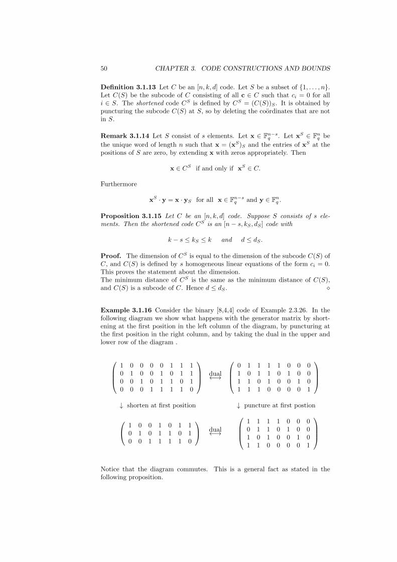
50 CHAPTER 3. CODE CONSTRUCTIONS AND BOUNDS
Definition 3.1.13 Let C be an [n, k, d] code. Let S be a subset of 1, . . . , n.Let C(S) be the subcode of C consisting of all c ∈ C such that ci = 0 for alli ∈ S. The shortened code CS is defined by CS = (C(S))S . It is obtained bypuncturing the subcode C(S) at S, so by deleting the coordinates that are notin S.
Remark 3.1.14 Let S consist of s elements. Let x ∈ Fn−sq . Let xS ∈ Fnq be
the unique word of length n such that x = (xS)S and the entries of xS at thepositions of S are zero, by extending x with zeros appropriately. Then
x ∈ CS if and only if xS ∈ C.
Furthermore
xS · y = x · yS for all x ∈ Fn−sq and y ∈ Fnq .
Proposition 3.1.15 Let C be an [n, k, d] code. Suppose S consists of s ele-ments. Then the shortened code CS is an [n− s, kS , dS ] code with
k − s ≤ kS ≤ k and d ≤ dS .
Proof. The dimension of CS is equal to the dimension of the subcode C(S) ofC, and C(S) is defined by s homogeneous linear equations of the form ci = 0.This proves the statement about the dimension.The minimum distance of CS is the same as the minimum distance of C(S),and C(S) is a subcode of C. Hence d ≤ dS .
Example 3.1.16 Consider the binary [8,4,4] code of Example 2.3.26. In thefollowing diagram we show what happens with the generator matrix by short-ening at the first position in the left column of the diagram, by puncturing atthe first position in the right column, and by taking the dual in the upper andlower row of the diagram .
1 0 0 0 0 1 1 10 1 0 0 1 0 1 10 0 1 0 1 1 0 10 0 0 1 1 1 1 0
dual←→
0 1 1 1 1 0 0 01 0 1 1 0 1 0 01 1 0 1 0 0 1 01 1 1 0 0 0 0 1
↓ shorten at first position ↓ puncture at first postion
1 0 0 1 0 1 10 1 0 1 1 0 10 0 1 1 1 1 0
dual←→
1 1 1 1 0 0 00 1 1 0 1 0 01 0 1 0 0 1 01 1 0 0 0 0 1
Notice that the diagram commutes. This is a general fact as stated in thefollowing proposition.
3.1. CODE CONSTRUCTIONS 51
Proposition 3.1.17 Let C be an [n, k, d] code. Let P and S be subsets of1, . . . , n. Then
(CP )⊥ = (C⊥)P and (CS)⊥ = (C⊥)S ,
dimCP + dim(C⊥)P = |P | and dimCS + dim(C⊥)S = |S|.
Proof. Let x ∈ (CP )⊥. Let z ∈ C. Then zP ∈ CP . So xP · z = x · zP = 0, byRemark 3.1.14. Hence xP ∈ C⊥ and x ∈ (C⊥)P . Therefore (CP )⊥ ⊆ (C⊥)P .Conversely, let x ∈ (C⊥)P . Then xP ∈ C⊥. Let y ∈ CP . Then y = zP forsome z ∈ C. So x · y = x · zP = xP · z = 0. Hence x ∈ (CP )⊥. Therefore(C⊥)P ⊆ (CP )⊥, and if fact equality holds, since the converse inclusion wasalready shown.The statement on the dimensions is a direct consequence of the correspondingequality of the codes.The claim about the shortening of C with S is a consequence on the equalityon the puncturing with S = P applied to the dual C.
If we want to increase the size of the code without changing the code length.We can augment the code by adding a word which is not in the code.
Definition 3.1.18 Let C be an Fq-linear code of length n. Let v in Fnq . Theaugmented code, denoted by Ca(v), is defined by
Ca(v) = αv + c | α ∈ Fq, c ∈ C .
If v is the all-ones vector, then we denote Ca(v) by Ca.
Remark 3.1.19 The augmented code Ca(v) is a linear code. Suppose that Gis a generator matrix of C. Then the (k+1)×n matrix Ga(v), which is obtainedby adding the row v to G, is a generator matrix of Ca(v) if v is not an elementof C.
Proposition 3.1.20 Let C be a code of minimum distance d. Suppose that thevector v is not in C and has weight w. Then
mind− w,w ≤ d(Ca(v)) ≤ mind,w.
In particular d(Ca(v)) = w if w ≤ d/2.
Proof. C is a subcode and v is an element of the augmented code. Thisimplies the upper bound.The lower bound is trivially satisfied if d ≤ w. Suppose w < d. Let x be anonzero element of Ca(v). Then x = αv + c for some α ∈ Fq and c ∈ C. Ifα = 0, then wt(x) = wt(c) ≥ d > w. If c = 0, then wt(x) = wt(v) = w.If α 6= 0 and c 6= 0, then c = αv − x. So d ≤ wt(c) ≤ w + wt(x). Henced− w ≤ wt(x).If w ≤ d/2, then the upper and lower bound are both equal to w.
Suppose C is a binary [n, k, d] code. We get a new code by deleting the code-words of odd weight. In other words, the new code Cev consists of all thecodewords in C which have even weight. It is called the even weight subcode inExample 2.2.8. This process is also called expurgating the code C.
52 CHAPTER 3. CODE CONSTRUCTIONS AND BOUNDS
Definition 3.1.21 Let C be an Fq-linear code of length n. Let v ∈ Fnq . Theexpurgated code of C is denoted by Ce(v) and is defined by
Ce(v) = c | c ∈ C and c · v = 0 .
If v = 1, then Ce(1) is denoted by Ce.
Proposition 3.1.22 Let C be an [n, k, d] code. Then
(Ca(v))⊥ = (C⊥)e(v).
Proof. If v ∈ C, then Ca(v) = C and v is a parity check of C, so (C⊥)e(v) =C⊥. Suppose v is not an element of C. Let G be a generator matrix of C.Then G is a parity check matrix of C⊥, by Proposition 2.3.29. Now Ga(v) is agenerator matrix of Ca(v) by definition. Hence Ga(v) is a parity check matrixof (Ca(v))⊥ Furthermore Ga(v) is also a parity check matrix of (C⊥)e(v) bydefinition. Hence (Ca(v))⊥ = (C⊥)e(v).
Lengthening a code is a technique which combines augmenting and extending.
Definition 3.1.23 Let C be an [n, k] code. Let v in Fnq . The lengthened
code Cl(v) is obtained by first augmenting C by v, and then extending it:Cl(v) = (Ca(v))e. If v = 1, then Cl(v) is denoted by Cl.
Remark 3.1.24 The lengthening of an [n,k] code is linear code. If v is notelement of C, then Cl(v) is an [n+ 1, k + 1] code.
3.1.2 Product codes
We describe a method for combining two codes to get a new code. In Example2.1.2 the [9,4,4] product code is introduced. This construction will be general-ized in this section.
Consider the identification of the space of all n1 × n2 matrices with entries inFq and the space Fnq , where the matrix X = (xij)1≤i≤n1,1≤j≤n2
is mapped tothe vector x with entries x(i−1)n2+j = xij . In other words, the rows of X areput in linear order behind each other:
x = (x11, x12, . . . , x1n2 , x21, . . . , x2n2 , x31, . . . , xn1n2).
For α ∈ Fq and n1 × n2 matrices (xij) and (yij) with entries in Fq, the scalarmultiplication and addition are defined by:
α(xij) = (αxij), and (xij) + (yij) = (xij + yij).
These operations on matrices give the corresponding operations of the vectorsunder the identification. Hence the identification of the space of n1×n2 matricesand the space Fnq is an isomorphism of vector spaces. In the following these twospaces are identified.
Definition 3.1.25 Let C1 and C2 be respectively [n1, k1, d1] and [n2, k2, d2]codes. Let n = n1n2. The product code, denoted by C1 ⊗ C2 is defined by
C1 ⊗ C2 =
(cij)1≤i≤n1,1≤j≤n2
∣∣∣∣ (cij)1≤i≤n1∈ C1, for all j
(cij)1≤j≤n2∈ C2, for all i
.
3.1. CODE CONSTRUCTIONS 53
From the definition, the product code C1 ⊗ C2 is exactly the set of all n1 × n2
arrays whose columns belong to C1 and rows to C2. In the literature, theproduct code is called direct product, or Kronecker product, or tensor productcode.
Example 3.1.26 Let C1 = C2 be the [3, 2, 2] binary even weight code. So itconsists of the following codewords:
(0, 0, 0), (1, 1, 0), (1, 0, 1), (0, 1, 1).
This is the set of all words (m1,m2,m1 + m2) where m1 and m2 are arbitrarybits. By the definition, the following 16 arrays are the codewords of the productcode C1 ⊗ C2: m1 m2 m1 +m2
m3 m4 m3 +m4
m1 +m3 m2 +m4 m1 +m2 +m3 +m4
,
where the mi are free to choose. So indeed this is the product code of Example2.1.2. The sum of two arrays (cij) and (c′ij) is the array (cij + c′ij). Therefore,C1 ⊗ C2 is a linear codes of length 9 = 3× 3 and dimension 4 = 2× 2. And itis clear that the minimum distance of C1 ⊗ C2 is 4 = 2× 2.
This is a general fact, but before we state this result we need some preparations.
Definition 3.1.27 For two vectors x = (x1, . . . , xn1) and y = (y1, . . . , yn2
), wedefine the tensor product of them, denoted by x⊗y, as the n1×n2 array whose(i, j)-entry is xiyj .
Remark 3.1.28 It is clear that C1 ⊗C2 is a linear code if C1 and C2 are bothlinear.Remark that x ⊗ y ∈ C1 ⊗ C2 if x ∈ C1 and y ∈ C2, since the i-th row ofx ⊗ y is xiy ∈ C2 and the j-th column is yjx
T and yjx ∈ C1. But the set ofall x ⊗ y ∈ C1 ⊗ C2 with x ∈ C1 and y ∈ C2 is not equal to C1 ⊗ C2. In theprevious example 0 1 1
1 0 11 1 0
is in the product code, but it is not of the form x⊗ y ∈ C1 ⊗ C2 with x ∈ C1,since otherwise it would have at least one zero row and at least one zero column.In general, the number of elements of the form x ⊗ y ∈ C1 ⊗ C2 with x ∈ C1
and y ∈ C2 is equal to qk1+k2 , but x ⊗ y = 0 if x = 0 or y = 0. Moreoverλ(x ⊗ y) = (λx) ⊗ y = x ⊗ (λy) for all λ ∈ Fq. Hence the we get at most(qk1 − 1)(qk2 − 1)/(q− 1) + 1 of such elements. If k1 > 1 and k2 > 1 then this issmaller than qk1k2 , the number of elements of C1⊗C2 according to the followingproposition.
Proposition 3.1.29 Let x1, . . . ,xk ∈ Fn1q and y1, . . . ,yk ∈ Fn2
q . If y1, . . . ,ykare independent and x1 ⊗ y1 + · · ·+ xk ⊗ yk = 0, then xi = 0 for all i.
Proof. Suppose that y1, . . . ,yk are independent and x1⊗y1+· · ·+xk⊗yk = 0.Let xis be the s-the entry of xi. Then the s-th row of
∑j xj ⊗ yj is equal to∑
j xjsyj , which is equal to 0 by assumption. Hence xjs = 0 for all j and s.Hence xj = 0 for all j.
54 CHAPTER 3. CODE CONSTRUCTIONS AND BOUNDS
Corollary 3.1.30 Let x1, . . . ,xk1∈ Fn1
q and y1, . . . ,yk2∈ Fn2
q . If x1, . . . ,xk1
and y1, . . . ,yk2are both independent, then xi ⊗ yj | 1 ≤ i ≤ k1, 1 ≤ j ≤ k2
is an independent set of matrices.
Proof. Suppose that∑i,j λijxi ⊗ yj = 0 for certain scalars λij ∈ Fq. Then∑
j(∑i λijxi)⊗yj = 0 and y1, . . . ,yk2
∈ Fn2q are independent. So
∑i λijxi = 0
for all j by Proposition 3.1.29. Hence λij = 0 for all i, j, since x1, . . . ,xk1are
independent.
Proposition 3.1.31 Let x1, . . . ,xk1in Fn1
q be a basis of C1 and y1, . . . ,yk2in
Fn2q a basis of C2. Then
xi ⊗ yj | 1 ≤ i ≤ k1, 1 ≤ j ≤ k2
is a basis of C1 ⊗ C2.
Proof. The given set is an independent set by Corollary 3.1.30. This set isa subset of C1 ⊗ C2. So the dimension of C1 ⊗ C2 is at least k1k2. Now wewill show that they form in fact a basis for C1 ⊗C2. Without loss of generalitywe may assume that C1 is systematic at the first k1 coordinates with generatormatrix (Ik1 |A) and C2 is systematic at the first k2 coordinates with generatormatrix (Ik2
|B). Then U is an l × n2 matrix, with rows in C2 if and only ifU = (M |MB), where M is an l× k2 matrix. And V is an n1 ×m matrix, withcolumns in C1 if and only if V T = (N |NA), where N is an m× k1 matrix. Nowlet M be an k1 × k2 matrix. Then (M |MB) is a k1 × n2 matrix with rows inC2, and (
MATM
)is an n1 × k2 matrix with columns in C1. Therefore(
M MBATM ATMB
)is an n1 × n2 matrix with columns in C1 and rows in C2 for every k1 × k2
matrix M . And conversely every codeword of C1⊗C2 is of this form. Hence thedimension of C1 ⊗C2 is equal to k1k2 and the given set is a basis of C1 ⊗C2.
Theorem 3.1.32 Let C1 and C2 be respectively [n1, k1, d1] and [n2, k2, d2].Then the product code C1 ⊗ C2 is an [n1n2, k1k2, d1d2] code.
Proof. By definition n = n1n2 is the length of the product code. It wasalready mentioned that C1 ⊗ C2 is a linear subspace of Fn1n2
q . The dimensionof the product code is k1k2 by Proposition 3.1.31.Next, we prove that the minimum distance of C1⊗C2 is d1d2. For any codewordof C1 ⊗ C2, which is a n1 × n2 array, every nonzero column has weight ≥ d1,and every nonzero row has weight ≥ d2. So, the weight of a nonzero codewordof the product code is at least d1d2. This implies that the minimum distance ofC1 ⊗ C2 is at least d1d2. Now suppose x ∈ C1 has weight d1, and y ∈ C2 hasweight d2. Then, x⊗ y is a codeword of C1 ⊗ C2 and has weight d1d2.
3.1. CODE CONSTRUCTIONS 55
Definition 3.1.33 Let A = (aij) be a k1 × n1 matrix and B = (bij) a k2 × n2
matrix. The Kronecker product or tensor product A ⊗ B of A and B is thek1k2 × n1n2 matrix obtained from A by replacing every entry aij by aijB.
Remark 3.1.34 The tensor product x ⊗ y of the two row vectors x and y oflength n1 and n2, respectively, as defined in Definition 3.1.27 is the same as theKronecker product of xT and y, now considered as n1 × 1 and 1× n2 matrices,respectively, as in Definition 3.1.33.
Proposition 3.1.35 Let G1 be a generator matrix of C1, and G2 a generatormatrix of C2. Then G1 ⊗G2 is a generator matrix of C1 ⊗ C2.
Proof. In this proposition the codewords are considered as elements of Fnq andno longer as matrices. Let xi the i-th row of G1, and denote by yj the j-th rowof G2. So x1, . . . ,xk1 ∈ Fn1
q is a basis of C1 and y1, . . . ,yk2 ∈ Fn2q is a basis of
C2. Hence the set xi ⊗ yj | 1 ≤ i ≤ k1, 1 ≤ j ≤ k2 is a basis of C1 ⊗ C2 byProposition 3.1.31. Furthermore, if l = (i − 1)k2 + j, then xi ⊗ yj is the l-throw of G1 ⊗G2. Hence the matrix G1 ⊗G2 is a generator matrix of C1 ⊗C2.
Example 3.1.36 Consider the ternary codes C1 and C2 with generator matri-ces
G1 =
(1 1 10 1 2
)and G2 =
1 1 1 00 1 2 00 1 1 1
,
respectively. Then
G1 ⊗G2 =
1 1 1 0 1 1 1 0 1 1 1 00 1 2 0 0 1 2 0 0 1 2 00 1 1 1 0 1 1 1 0 1 1 10 0 0 0 1 1 1 0 2 2 2 00 0 0 0 0 1 2 0 0 2 1 00 0 0 0 0 1 1 1 0 2 2 2
.
The second row of G1 is x2 = (0, 1, 2) and y2 = (0, 1, 2, 0) is the second row ofG2. Then x2 ⊗ y2 is equal to 0 0 0 0
0 1 2 00 2 1 0
,
considered as a matrix, and equal to (0, 0, 0, 0, 0, 1, 2, 0, 0, 2, 1, 0) written as avector, which is indeed equal to the (2− 1)3 + 2 = 5-th row of G1 ⊗G2.
3.1.3 Several sum constructions
We have seen that given an [n1, k1] code C1 and an [n2, k2] code C2, by theproduct construction, we get an [n1n2, k1k2] code. The product code has infor-mation rate (k1k2)/(n1n2) = R1R2, where R1 and R2 are the rates of C1 andC2, respectively. In this subsection, we introduce some simple constructions bywhich we can get new codes with greater rate from two given codes.
56 CHAPTER 3. CODE CONSTRUCTIONS AND BOUNDS
Definition 3.1.37 Given an [n1, k1] code C1 and an [n2, k2] code. Their directsum C1 ⊕ C2, also called (u|v) construction is defined by
C1 ⊕ C2 = (u|v) | u ∈ C1,v ∈ C2 ,
where (u|v) denotes the word (u1, . . . , un1, v1, . . . , vn2
) if u = (u1, . . . , un1) and
v = (v1, . . . , vn2).
Proposition 3.1.38 Let Ci be an [ni, ki, di] code with generator matrix Gi fori = 1, 2. Let d = mind1, d2. Then C1⊕C2 is an [n1 +n2, k1 + k2, d] code withgenerator matrix
G =
(G1 00 G2
).
Proof. Let x1, . . . ,xk1and y1, . . . ,yk2
be bases of C1 and C2, respectively.Then (x1|0), . . . , (xk1 |0), (0|y1), . . . , (0|yk2) is a basis of the direct sum code.Therefore, the direct sum is an [n1 +n2, k1 +k2] with the given generator matrixG. The minimum distance of the direct sum is mind1, d2.
The direct sum or (u|v) construction is defined by the juxtaposition of arbitrarycodewords u ∈ C1 and v ∈ C2. In the following definition only a restricted setpairs of codewords are put behind each other. This definition depends on thechoice of the generator matrices of the codes C1 and C2.
Definition 3.1.39 Let C1 be an [n1, k, d1] code and C2 an [n2, k, d2] code withgenerator matrices G1 and G2, respectively. The juxtaposition of the codes C1
and C2 is the code with generator matrix (G1|G2).
Proposition 3.1.40 Let Ci be an [ni, k, di] code for i = 1, 2. Then the juxta-position of the codes C1 and C2 is an [n1 + n2, k, d] with d ≥ d1 + d2.
Proof. The length and the dimension are clear from the definition. A nonzerocodeword c is of the form mG = (mG1,mG2) for a nonzero element m in Fkq .So mGi is a nonzero codeword of Ci. Hence the weight of c is at least d1 + d2.
The rate of the direct sum is (k1+k2)/(n1+n2), which is greater than (k1k2)/(n1n2),the rate of the product code. Now a more intelligent construction is studied.
Definition 3.1.41 Let C1 be an [n, k1, d1] code and C2 an [n, k2, d2] code,respectively. The (u|u + v) construction is the following code
( u|u + v) | u ∈ C1,v ∈ C2 .
Theorem 3.1.42 Let Ci be an [n, ki, di] code with generator matrix Gi fori = 1, 2. Then the (u|u + v) construction of C1 and C2 is an [2n, k1 + k2, d]code with minimum distance d = min2d1, d2 and generator matrix
G =
(G1 G1
0 G2
).
3.1. CODE CONSTRUCTIONS 57
Proof. It is straightforward to check the linearity of the (u|u+v) construction.Suppose x1, . . . ,xk1
and y1, . . . ,yk2are bases of C1 and C2, respectively. Then,
it is easy to see that (x1|x1), . . . , (xk1|xk1
), (0|y1), . . . , (0|yk2) is a basis of the
(u|u+v) construction. So, it is an [2n, k1+k2] with generator matrix G as given.
Consider the minimum distance d of the (u|u + v) construction. For any code-word (x|x + y), we have wt(x|x + y) = wt(x) + wt(x + y). If y = 0, thenwt(x|x + y) = 2wt(x) ≥ 2d1. If y 6= 0, then
wt(x|x + y) = wt(x) + wt(x + y) ≥ wt(x) + wt(y)− wt(x) = wt(y) ≥ d2.
Hence, d ≥ min2d1, d2. Let x0 be a codeword of C1 with weight d1, and y0
be a codeword of C2 with weight d2. Then, either (x0|x0) or (0|y0) has weightmin2d1, d2.
Example 3.1.43 The (u|u + v) construction of the binary even weight [4,3,2]code and the 4-tuple repetition [4,1,4] code gives a [8,4,4] code with generatormatrix
1 0 0 1 1 0 0 10 1 0 1 0 1 0 10 0 1 1 0 0 1 10 0 0 0 1 1 1 1
,
which is equivalent with the extended Hamming code of Example 2.3.26.
Remark 3.1.44 For two vectors u of length n1 and v of length n2, we can stilldefine the sum u + v as a vector of length maxn1, n2, by adding enough zerosat the end of the shorter vector. From this definition of sum, the (u|u + v)construction still works for codes C1 and C2 of different lengths.
Proposition 3.1.45 If C1 is an [n1, k1, d1] code, and C2 is an [n2, k2, d2] code,then the (u|u + v) construction is an [n1 + maxn1, n2, k1 + k2,min2d1, d2]linear code.
Proof. The proof is similar to the proof of Theorem 3.1.42.
Definition 3.1.46 The (u + v|u − v) construction is a slightly modified con-struction, which is defined as the following code
(u + v|u− v) | u ∈ C1,v ∈ C2 .
When we consider this construction, we restrict ourselves to the case q odd.Since u + v = u− v if q is even.
Proposition 3.1.47 Let Ci be an [n, ki, di] code with generator matrix Gi fori = 1, 2. Assume that q is odd. Then, the (u + v|u− v) construction of C1 andC2 is an [2n, k1 +k2, d] code with d ≥ min2d1, 2d2,maxd1, d2 and generatormatrix
G =
(G1 G1
G2 −G2
).
58 CHAPTER 3. CODE CONSTRUCTIONS AND BOUNDS
Proof. The proof of the proposition is similar to that of Theorem 3.1.42. Infact, suppose x1, . . . ,xk1
and y1, . . . ,yk2are bases of C1 and C2, respectively,
then every codeword is of the form (u + v|u − v) = (u|u) + (v| − v). Withu ∈ C1 and v ∈ C2. So (u|u) is a linear combination of (x1|x1), . . . , (xk1 |xk1),and (v| − v) is a linear combination of (y1| − y1), . . . , (yk2 | − yk2).Using the assumption that q is odd, we can prove that this set of vectors (xi|xi),(yj | − yj) is linearly independent. Suppose that∑
i
λi(xi|xi) +∑j
µj(yj | − yj) = 0,
Then ∑i λixi +
∑j µjyj = 0,∑
i λixi −∑j µjyj = 0.
Adding the two equations and dividing by 2 gives∑i λixi = 0. So λi = 0 for
all i, since the xi are independent. Similarly, the substraction of the equationsgives that µj = 0 for all j.So the (xi|xi), (yj | − yj) are independent and generate the code. Hence theyform a basis and this shows that the given G is a generator matrix of thisconstruction.Let (u + v|u − v) be a nonzero codeword. The weight of this word is at least2d1 if v = 0, and at least 2d2 if u = 0. Now suppose u 6= 0 and v 6= 0. Thenthe weight of u− v is at least wt(u)− w, where w is the number of positions isuch that ui = vi 6= 0. If ui = vi 6= 0, then ui + vi 6= 0, since q is odd. Hencewt(u + v) ≥ w, and (u + v|u − v) ≥ w + (wt(u) − w) = wt(u) ≥ d1. In thesame way wt(u + v|u − v) ≥ d2. Hence wt(u + v|u − v) ≥ maxd1, d2. Thisproofs the estimate on the minimum distance.
Example 3.1.48 Consider the following ternary codes
C1 = 000, 110, 220, C2 = 000, 011, 022.
They are [3, 1, 2] codes. The (u + v|u − v) construction of these codes is a[6, 2, d] code with d ≥ 2 by Proposition 3.1.47. It consists of the following ninecodewords:
(0, 0, 0, 0, 0, 0), (0, 1, 1, 0, 2, 2), (0, 2, 2, 0, 1, 1),(1, 1, 0, 1, 1, 0), (1, 2, 1, 1, 0, 2), (1, 0, 2, 1, 2, 1),(2, 2, 0, 2, 2, 0), (2, 0, 1, 2, 1, 2), (2, 1, 2, 2, 0, 1).
Hence d = 4. On the other hand, by the (u|u+v) construction, we get a [6, 2, 2]code, which has a smaller minimum distance than the (u+v|u−v) construction.
Now a more complicated construction is given.
Definition 3.1.49 Let C1 and C2 be [n, k1] and [n, k2] codes, respectively. The(a + x|b + x|a + b− x) construction of C1 and C2 is the following code
(a + x|b + x|a + b− x) | a,b ∈ C1,x ∈ C2
3.1. CODE CONSTRUCTIONS 59
Proposition 3.1.50 Let C1 and C2 be [n, k1] and [n, k2] codes over Fq, re-spectively. Suppose q is not a power of 3. Then, the (a + x|b + x|a + b − x)construction of C1 and C2 is an [3n, 2k1 + k2] code with generator matrix
G =
G1 0 G1
0 G1 G1
G2 G2 −G2
.
Proof. Let x1, . . . ,xk1and y1, . . . ,yk2
be bases of C1 and C2, respectively.Consider the following 2k1 + k2 vectors
(x1|0|x1), . . . , (xk1|0|xk1
),
(0|x1|x1), . . . , (0|xk1 |xk1),
(y1|y1| − y1), . . . , (yk2|yk2| − yk2
).
It is left as an exercise to check that they form a basis of this construction incase q is not a power of 3. This shows that the given G is a generator matrix ofthe code and that it dimension is 2k1 + k2.
For binary codes, some simple inequalities, for example, Exercise 3.1.9, can beused to estimate the minimum distance of the last construction. In general wehave the following estimate for the minimum distance.
Proposition 3.1.51 Let C1 and C2 be [n, k1, d1] and [n, k2, d2] codes over Fq,respectively. Suppose q is not a power of 3. Let d0 and d3 be the minimumdistance of C1∩C2 and C1 +C2, respectively. Then, the minimum distance d ofthe (a+x|b+x|a+b−x) construction of C1 and C2 is at least mind0, 2d1, 3d3.
Proof. This is left as an exercise.
The choice of the minus sign in the (a + x|b + x|a + b − x) construction be-comes apparent in the construction of self-dual codes over Fq for arbitrary q notdivisible by 3.
Proposition 3.1.52 Let C1 and C2 be self-dual [2k,k] codes. The the codesobtained from C1 and C2 by the direct sum, the (u|u + v) if C1 = C2, and the(u+v|u−v) constructions and the (a+x|b+x|a+b−x) construction in caseq is not divisible by 3 are also self-dual.
Proof. The generator matrix Gi of Ci has size k × 2k and satisfies GiGTi = 0
for i = 1, 2. In all the constructions the generator matrix G has size 2k × 4k or3k × 6k as given in Theorem 3.1.42 and Propositions 3.1.38, 3.1.48 and 3.1.50satisfies also GGT = 0. For instance in the case of the (a + x|b + x|a + b− x)construction we have
GGT =
G1 0 G1
0 G1 G1
G2 G2 −G2
GT1 0 GT20 GT1 GT2GT1 GT1 −GT2
.
All the entries in this product are the sum of terms of the form GiGTi or G1G
T2 −
G1GT2 which are all zero. Hence GGT = 0.
60 CHAPTER 3. CODE CONSTRUCTIONS AND BOUNDS
Example 3.1.53 Let C1 be the binary [8, 4, 4] self-dual code with the generatormatrix G1 of the form (I4|A1) as given in Example 2.3.26. Let C2 be the codewith generator matrix G2 = (I4|A2) where A2 is obtained from A1 by a cyclicshift of the columns.
A1 =
0 1 1 11 0 1 11 1 0 11 1 1 0
, A2 =
1 0 1 11 1 0 11 1 1 00 1 1 1
.
The codes C1 and C2 are both [8, 4, 4] self-dual codes and C1 ∩C2 = 0,1 andC1+C2 is the even weight code. Let C be the (a+x|b+x|a+b+x) constructionapplied to C1 and C2. Then C is a binary self-dual [24, 12, 8] code. The claim onthe minimum distance is the only remaining statement to verify, by Proposition3.1.52. Let G be the generator matrix of C as given in Proposition 3.1.50. Theweights of the rows of G are all divisible by 4. Hence the weights of all codewordsare divisible by 4 by Exercise ??. Let c = (a + x|b + x|a + b + x) be a nonzerocodeword with a,b ∈ C1 and x ∈ C2. If a + x = 0, then a = x ∈ C1 ∩ C2. Soa = x = 0 and c = (0|b|b) or a = x = 1
¯and c = (0|b + 1|b), and in both cases
the weight of c is at least 8, since the weight of b is at least 4 and the weightof 1 is 8. Similarly it is argued that the weight of c is at least 8 if b + x = 0 ora + b + x = 0. So we may assume that neither of a + x, b + x, nor a + b + xis zero. Hence all three are nonzero even weight codewords and wt(c) ≥ 6. Butthe weight is divisible by 4. Hence the minimum distance is at least 8. Let abe a codeword of C1 of weight 4, then c = (a, 0,a) is a codeword of weight 8.In this way we have constructed a binary self-dual [24, 12, 8] code. It is calledthe extended binary Golay code. The binary Golay code is the [23, 12, 7] codeobtained by puncturing one coordinate.
3.1.4 Concatenated codes
For this section we need some theory of finite fields. See Section 7.2.1. Let qbe a prime power and k a positive integer. The finite field Fqk with qk elementscontains Fq as a subfield. Now Fqk is a k-dimensional vector over Fq. Letξ1, . . . , ξk be a basis of Fqk over Fq.Consider the map
ϕ : Fkq −→ Fqk .defined by ϕ(a) = a1ξ1 + · · ·+ akξk. Then ϕ is an isomorphism of vector spaceswith inverse map ϕ−1.The vector space FK×kq of K×k matrices over Fq form a vector space of dimen-
sion Kk over Fq and it is linear isometric with FKkq by taking some ordering ofthe Kk entries of such matrices. Let M be a K × k matrix over Fq with i-throw mi. The map
ϕK : FK×kq −→ FKqkis defined by ϕK(M) = (ϕ(m1), . . . , ϕ(mK)). The inverse map
ϕ−1N : FNqk −→ FN×kq
is given by ϕ−1N (a1, . . . ,an) = P , where P is the N × k matrix with i-th row
pi = ϕ−1(ai).
3.1. CODE CONSTRUCTIONS 61
Let A be an [N,K] code over Fqk , and B an [n, k] code over Fq. Let GA andGB be generator matrices of A and B, respectively. The N -fold direct sum
G(N)B = GB ⊕ · · · ⊕GB : FNkq → FNnq is defined by G
(N)B (P ) which is the N × n
matrix Q with i-th row qi = piGB for a given N × k matrix P with i-th rowpi in Fkq .
By the following concatenation procedure a message of length Kk over Fq isencoded to a codeword of length Nn over Fq.
Step 1: The K × k matrix M is mapped to m = ϕK(M).
Step 2: m in FKqk is mapped to a = mGA in FNqk .
Step 3: a in FNqk is mapped to P = ϕ−1N (a).
Step 4: The N × k matrix P with i-th row pi is mapped to the N × n matrixQ with i-th row qi = piGB .
The encoding mapE : FK×kq −→ FN×nq
is the composition of the four maps explained above:
E = G(N)B ϕ−1
N GA ϕK .
LetC = E(M) | M ∈ FK×kq .
We call C the concatenated code with outer code A and inner code B.
Theorem 3.1.54 Let A be an [N,K,D] code over Fqk , and B an [n, k, d] codeover Fq. Let C be the concatenated code with outer code A and inner code B.Then C is an Fq-linear [Nn,Kk] code and its minimum distance is at least Dd.
Proof. The encoding map E is an Fq-linear map, since it is a composition offour Fq-linear maps. The first and third map are isomorphisms, and the secondand last map are injective, since they are given by generator matrices of fullrank. Hence E is injective. Hence the concatenated code C is an Fq-linear codeof length Nn and dimension Kk.Next, consider the minimum distance of C. Since A is an [N,K,D] code, everynonzero codeword a obtained in Step 2 has weight at least D. As a result,the N × k matrix P obtained from Step 3 has at least D nonzero rows pi.Now, because B is a [n, k, d] code, every piGB has weight d, if pi is not zero.Therefore, the minimum distance of C is at least Dd.
Example 3.1.55 The definition of the concatenated code depends on the choiceof the map ϕ that is on the choice of the basis ξ1, . . . , ξn. In fact the minimumdistance of the concatenated code can be strictly larger than Dd as the followingexample shows.The field F9 contains the ternary field F3 as a subfield and an element ξ suchthat ξ2 = 1 + ξ, since the polynomial X2 −X − 1 is irreducible in F3[X]. Nowtake ξ1 = 1 and ξ2 = ξ as a basis of F9 over F3. Let A be the [2, 1, 2] outer code
62 CHAPTER 3. CODE CONSTRUCTIONS AND BOUNDS
over F9 with generator matrix GA = [1, ξ2]. Let B be the trivial [2, 2, 1] codeover F3 with generator matrix GB = I2. Let M = (m1,m2) ∈ F1×2
3 . Then m =ϕ1(M) = m1 +m2ξ ∈ F9. So a = mGA = (m1 +m2ξ, (m1 +m2)+(m1−m2)ξ),since ξ3 = 1− ξ. Hence
Q = P = ϕ−12 (a) =
(m1 m2
m1 +m2 m1 −m2
).
Therefore the concatenated code has minimum distance 3 > Dd.Suppose we would have taken ξ′1 = 1 and ξ′2 = ξ2 as a basis instead. TakeM = (1, 0). Then m = ϕ1(M) = 1 ∈ F9. So a = mGA = (1, ξ2). HenceQ = P = ϕ−1
2 (a) = I2 is a codeword in the concatenated code that has weight2 = Dd.Thus, the definition and the parameters of a concatenated code dependent onthe specific choice of the map ϕ.
3.1.5 Exercises
3.1.1 Prove Proposition 3.1.11.
3.1.2 Let C be the binary [9,4,4] product code of Example 2.1.2. Show thatpuncturing C at the position i gives a [8,4,3] code for every choice of i = 1, . . . , 9.Is it possible to obtain the binary [7,4,3] Hamming code by puncturing C? Showthat shortening C at the position i gives a [8,3,4] code for every choice of i.Is it possible to obtain the binary [7,3,4] Simplex code by a combination ofpuncturing and shortening the product code?
3.1.3 Suppose that there exists an [n′, k′, d′]q code and an [n, k, d]q code witha [n, k− k′, d+ d′]q subcode. Use a generalization of the construction for Ce(v)to show that there exists an [n+ n′, k, d+ d′]q code.
3.1.4 Let C be a binary code with minimum distance d. Let d′ be the largestweight of any codeword of C. Suppose that the all-ones vector is not in C.Then, the augmented code Ca has minimum distance mind, n− d′.
3.1.5 Let C be an Fq-linear code of length n. Let v ∈ Fnq and S = n + 1.Suppose that the all-ones vector is a parity check of C but not of v. Show that(Cl(c))S = C.
3.1.6 Show that the shortened binary [7,3,4] code is a product code of codesof length 2 and 3.
3.1.7 Let C be a nontrivial linear code of length n. Then C is the direct sumof two codes of lengths strictly smaller than n if and only if C = v ∗C for somev ∈ Fnq with nonzero entries that are not all the same.
3.1.8 Show that the punctured binary [7,3,4] is equal to the (u|u + v) con-struction of a [3, 2, 2] code and a [3, 1, 3] code.
3.1.9 For binary vectors a, b and x,
wt(a + x|b + x|a + b + x) ≥ 2wt(a + b + a ∗ b)− wt(x),
with equality if and only if ai = 1 or bi = 1 or xi = 0 for all i, where a ∗ b =(a1b1, . . . , anbn).
3.2. BOUNDS ON CODES 63
3.1.10 Give a parity check matrix for the direct sum, the (u|u + v), the (u +v|u − v) and the (a + x|b + x|a + b − x) construction in terms of the paritycheck matrices H1 and H2 of the codes C1 and C2, respectively.
3.1.11 Give proofs of Propositions 3.1.50 and 3.1.51.
3.1.12 Let Ci be an [n, ki, di] code over Fq for i = 1, 2, where q is a power of3. Let k0 be the dimension of C1∩C2 and d3 the minimum distance of C1 +C2.Show that the (a + x|b + x|a + b − x) construction with C1 and C2 gives a[3n, 2k1 + k2 − k0, d] code with d ≥ min2d1, 3d3.
3.1.13 Show that C1 ∩ C2 = 0,1 and C1 + C2 is the even weight code, forthe codes C1 and C2 of Example 3.1.53.
3.1.14 Show the existence of a binary [45,15,16] code.
3.1.15 Show the existence of a binary self-dual [72,36,12] code.
3.1.16 [CAS] Construct a binary random [100, 50] code and make sure thatidentities from Proposition 3.1.17 take place for different position sets: the lastposition, the last five, the random five.
3.1.17 [CAS] Write procedures that take generator matrices G1 and G2 of thecodes C1 and C2 and return a matrix G that is the generator matrix of the codeC, which is the result of the
• (u + v|u− v)-construction of Proposition 3.1.47;
• (a + x|b + x|a + b− x)-construction of Proposition 3.1.50.
3.1.18 [CAS] Using the previous exercise construct the extended Golay code asin Example 3.1.53. Compare this code with the one returned by ExtendedBinary
GolayCode() (in GAP) and GolayCode(GF(2),true) (in Magma).
3.1.19 Show by means of an example that the concatenation of an [3, 2, 2]outer and [, 2, 2, 1] inner code gives a [6, 4] code of minimum distance 2 or 3depending on the choice of the basis of the extended field.
3.2 Bounds on codes
We have introduced some parameters of a linear code in the previous sections.In coding theory one of the most basic problems is to find the best value of aparameter when other parameters have been given. In this section, we discusssome bounds on the code parameters.
3.2.1 Singleton bound and MDS codes
The following bound gives us the maximal minimum distance of a code with agiven length and dimension. This bound is called the Singleton bound.
Theorem 3.2.1 (The Singleton Bound) If C is an [n, k, d] code, then
d ≤ n− k + 1.
64 CHAPTER 3. CODE CONSTRUCTIONS AND BOUNDS
Proof. Let H be a parity check matrix of C. This is an (n− k)×n matrix ofrow rank n− k. The minimum distance of C is the smallest integer d such thatH has d linearly dependent columns, by Proposition 2.3.11. This means thatevery d− 1 columns of H are linearly independent. Hence, the column rank ofH is at least d− 1. By the fact that the column rank of a matrix is equal to therow rank, we have n− k ≥ d− 1. This implies the Singleton bound.
Definition 3.2.2 Let C be an [n, k, d] code. If d = n− k + 1, then C is calleda maximum distance separable code or an MDS code, for short.
Remark 3.2.3 From the Singleton bound, a maximum distance separable codeachieves the maximum possible value for the minimum distance given the codelength and dimension.
Example 3.2.4 The minimum distance of the the zero code of length n is n+1,by definition. Hence the zero code has parameters [n, 0, n+ 1] and is MDS. Itsdual is the whole space Fnq with parameters [n, n, 1] and is also MDS. The n-foldrepetition code has parameters [n, 1, n] and its dual is an [n, n− 1, 2] code andboth are MDS.
Proposition 3.2.5 Let C be an [n, k, d] code over Fq. Let G be a generatormatrix and H a parity check matrix of C. Then the following statements areequivalent:(1) C is an MDS code,(2) every (n− k)-tuple of columns of a parity check matrix H are linearly inde-pendent,(3) every k-tuple of columns of a generator matrix G are linearly independent.
Proof. As the minimum distance of C is d any d−1 columns of H are linearlyindependent, by Proposition 2.3.11. Now d ≤ n−k+ 1 by the Singleton bound.So d = n−k+1 if and only if every n−k columns of H are independent. Hence(1) and (2) are equivalent.Now let us assume (3). Let c be an element of C which is zero at k givencoordinates. Let c = xG for some x ∈ Fkq . Let G′ be the square matrixconsisting of the k columns of G corresponding to the k given zero coordinatesof c. Then xG′ = 0. Hence x = 0, since the k columns of G′ are independentby assumption. So c = 0. This implies that the minimum distance of C is atleast n− (k − 1) = n− k + 1. Therefore C is an [n, k, n− k + 1] MDS code, bythe Singleton bound.Assume that C is MDS. Let G be a generator matrix of C. Let G′ be the squarematrix consisting of k chosen columns of G. Let x ∈ Fkq such that xG′ = 0.Then c = xG is codeword and its weight is at most n− k. So c = 0, since theminimum distance is n−k+1. Hence x = 0, since the rank of G is k. Thereforethe k columns are independent.
Example 3.2.6 Consider the code C over F5 of length 5 and dimension 2 withgenerator matrix
G =
(1 1 1 1 10 1 2 3 4
).
3.2. BOUNDS ON CODES 65
Note that while the first row of the generator matrix is the all 1’s vector, theentries of the second row are distinct. Since every codeword of C is a linearcombination of the first and second row, the minimum distance of C is at least5. On the other hand, the second row is a word of weight 4. Hence C is a [5, 2, 4]MDS code. The matrix G is a parity check matrix for the dual code C⊥. Allcolumns of G are nonzero, and every two columns are independent since
det
(1 1i j
)= j − i 6= 0
for all 0 ≤ i < j ≤ 4. Therefore, C⊥ is also an MDS code.
In fact, we have the following general result.
Corollary 3.2.7 The dual of an [n, k, n−k+1] MDS code is an [n, n−k, k+1]MDS code.
Proof. The trivial codes are MDS and are dual of each other by Example3.2.4. Assume 0 < k < n. Let H be a parity check matrix of an [n, k, n− k+ 1]MDS code C. Then any n − k columns of H are linearly independent, by (2)of Proposition 3.2.5. Now H is a generator matrix of the dual code. ThereforeC⊥ is an [n, n− k, k + 1] MDS code, since (3) of Proposition 3.2.5 holds.
Definition 3.2.8 Let a be a vector of Fkq . Then V (a) is the Vandermonde
matrix with entries ai−1j .
Lemma 3.2.9 Let a be a vector of Fkq . Then
detV (a) =∏
1≤r<s≤k
(ais − air ).
Proof. This is left as an exercise.
Proposition 3.2.10 Let n ≤ q. Let a = (a1, . . . , an) be an n-tuple of mutuallydistinct elements of Fq. Let k be an integer such that 0 ≤ k ≤ n. Define thematrices Gk(a) and G′k(a) by
Gk(a) =
1 · · · 1a1 · · · an...
. . ....
ak−11 · · · ak−1
n
and G′k(a) =
1 · · · 1 0a1 · · · an 0...
. . ....
...
ak−11 · · · ak−1
n 1
.
The codes with generator matrix Gk(a) and G′k(a) are MDS codes.
Proof. Consider a k × k submatrix of G(a). Then this is a Vandermondematrix and its determinant is not zero by Lemma 3.2.9, since the ai are mutuallydistinct. So any system of k columns of Gk(a) is independent. Hence Gk(a) isthe generator matrix of an MDS code by Proposition 3.2.5.The proof for G′k(a) is similar and is left as an exercise.
66 CHAPTER 3. CODE CONSTRUCTIONS AND BOUNDS
Remark 3.2.11 The codes defined in Proposition 3.2.10 are called generalizedReed-Solomon codes and are the prime examples of MDS codes. These codes willbe treated in Section 8.1. The notion of an MDS code has a nice interpretationof n points in general position in projective space as we will see in Section4.3.1. The following proposition shows the existence of MDS codes over Fqwith parameters [n, k, n − k + 1] for all possible values of k and n such that0 ≤ k ≤ n ≤ q + 1.
Example 3.2.12 Let q be a power of 2. Let n = q+ 2 and a1, a2, . . . , aq be anenumeration of the elements of Fq. Consider the code C with generator matrix
1 1 . . . 1 0 0a1 a2 . . . aq 0 1
a21 a2
2 . . . a2q 1 0
Then any 3 columns of this matrix are independent, since by the Proposition3.2.10, the only remaining nontrivial case to check is∣∣∣∣∣∣
1 1 0ai aj 1a2i a2
j 0
∣∣∣∣∣∣ = −(a2j − a2
i ) = (ai − aj)2 6= 0, in characteristic 2
for all 1 ≤ i < j ≤ q − 1. Hence C is a [q + 2, 3, q] code.
Remark 3.2.13 From (3) of Proposition 3.2.5 and Proposition 2.2.22 we seethat any k symbols of the codewords of an MDS code of dimension k may betaken as message symbols. This is another reason for the name of maximumdistance separable codes.
Corollary 3.2.14 Let C be an [n, k, d] code. Then C is MDS if and only iffor any given d coordinate positions i1, i2, . . . , id, there is a minimum weightcodeword with the set of these positions as support. Furthermore two codewordsof an MDS code of minimum weight with the same support are a nonzero multipleof each other.
Proof. Let G be a generator matrix of C. Suppose d < n − k + 1. Thereexist k positions j1, j2, . . . , jk such that the columns of G at these positions areindependent. The complement of these k positions consists of n − k elementsand d ≤ n−k. Choose a subset i1, i2, . . . , id of d elements in this complement.Let c be a codeword with support that is contained in i1, i2, . . . , id. Then c iszero at the positions j1, j2, . . . , jk. Hence c = 0 and the support of c is empty.If C is MDS, then d = n−k+1. Let i1, i2, . . . , id be a set of d coordinate posi-tions. Then the complement of this set consists of k−1 elements j1, j2, . . . , jk−1.Let jk = i1. Then j1, j2, . . . , jk are k elements that can be used for systematicencoding by Remark 3.2.13. So there is a unique codeword c such that cj = 0for all j = j1, j2, . . . , jk−1 and cjk = 1. Hence c is a nonzero codeword of weightat most d and support contained in i1, i2, . . . , id. Therefore c is a codewordof weight d and support equal to i1, i2, . . . , id, since d is the minimum weightof the code.Furthermore, let c′ be another codeword of weight d and support equal to
3.2. BOUNDS ON CODES 67
i1, i2, . . . , id. Then c′j = 0 for all j = j1, j2, . . . , jk−1 and c′jk 6= 0. Then c′ andc′jkc are two codewords that coincide at j1, j2, . . . , jk. Hence c′ = c′jkc.
Remark 3.2.15 It follows from Corollary 3.2.14 that the number of nonzerocodewords of an [n, k] MDS code of minimum weight n− k + 1 is equal to
(q − 1)
(n
n− k + 1
).
In Section 4.1, we will introduce the weight distribution of a linear code. Usingthe above result the weight distribution of an MDS code can be completelydetermined. This will be determined in Proposition 4.4.22.
Remark 3.2.16 Let C be an [n, k, n− k+ 1 code. Then it is systematic at thefirst k positions. Hence C has a generator matrix of the form (Ik|A). It is leftas an exercise to show that every square submatrix of A is nonsingular. Theconverse is also true.
Definition 3.2.17 Let n ≤ q. Let a, b, r and s be vectors of Fkq such thatai 6= bj for all i, j. Then C(a,b) is the k × k Cauchy matrix with entries1/(ai− bj), and C(a,b; r, s) is the k× k generalized Cauchy matrix with entriesrisj/(ai − bj). Let k be an integer such that 0 ≤ k ≤ n. Let A(a) be thek× (n−k) matrix with entries 1/(aj+k−ai) for 1 ≤ i ≤ k, 1 ≤ j ≤ n−k. Thenthe Cauchy code Ck(a) is the code with generator matrix (Ik|A(a)). If ri is notzero for all i, then A(a, r) is the k × (n− k) matrix with entries
rj+kr−1i
aj+k − aifor 1 ≤ i ≤ k, 1 ≤ j ≤ n− k.
The generalized Cauchy code Ck(a, r) is the code with generator matrix (Ik|A(a, r)).
Lemma 3.2.18 Let a, b, r and s be vectors of Fkq such that ai 6= bj for all i, j.Then
detC(a,b; r, s) =
n∏i=1
ri
n∏j=1
sj
∏i<j(ai − aj)(bj − bi)∏n
i,j=1(ai − bj).
Proof. This is left as an exercise.
Proposition 3.2.19 Let n ≤ q. Let a be an n-tuple of mutually distinct ele-ments of Fq, and r an n-tuple of nonzero elements of Fq. Let k be an integer suchthat 0 ≤ k ≤ n. Then the generalized Cauchy code Ck(a, r) is an [n, k, n−k+1]code.
Proof. Every square t × t submatrix of A is Cauchy matrix of the formC((ai1 , . . . , ait), (ak+j1 , . . . , ak+jt); (b−1
i1, . . . , b−1
it), (bk+j1 , . . . , bk+jt)). The deter-
minant of this matrix is not zero by Lemma 3.2.18, since the entries of a aremutually distinct and the entries of r are not zero. Hence (Ik|A(a, r)) is thegenerator matrix of an MDS code by Remark 3.2.16.
In Section 8.1 it will be shown that generalized Reed-Solomon codes and Cauchycodes are the same.
68 CHAPTER 3. CODE CONSTRUCTIONS AND BOUNDS
3.2.2 Griesmer bound
Clearly, the Singleton bound can be viewed as a lower bound on the code lengthn with given dimension k and minimum distance d, that is n ≥ d + k − 1. Inthis subsection, we will give another lower bound on the length.
Theorem 3.2.20 (The Griesmer Bound) If C is an [n, k, d] code with k >0, then
n ≥k−1∑i=0
⌈d
qi
⌉.
Note that the Griesmer bound implies the Singleton bound. In fact, we havedd/q0e = d and dd/qie ≥ 1 for i = 1, . . . , k − 1, which follow the Singletonbound. In the previous Section 3.1 we introduced some methods to constructnew codes from a given code. In the following, we give another construction ofa new code, which will be used to prove Theorem 3.2.20.
Let C be an [n, k, d] code, and c be a codeword with w = wt(c). Let I = supp(c)(see the definition in Subsection 2.1.2). The residual code of C with respect to c,denoted by Res(C, c), is the code of length n−w punctured on all the coordinatesof I.
Proposition 3.2.21 Suppose C is an [n, k, d] code over Fq and c is a codewordof weight w < (qd)/(q − 1). Then Res(C, c) is an [n− w, k − 1, d′] code with
d′ ≥ d− w +
⌈w
q
⌉.
Proof. By replacing C by an equivalent code we may assume without loss ofthe generality that c = (1, 1, . . . , 1, 0, . . . , 0) where the first w components areequal to 1 and other components are 0. Clearly, the dimension of Res(C, c) isless than or equal to k − 1. If the dimension is strictly less than k − 1, thenthere must be a nonzero codeword in C of the form x = (x1, . . . , xw, 0, . . . , 0),where not all the xi are the same. There exists α ∈ Fq such that at least w/qcoordinates of (x1, . . . , xw) equal to α. Thus,
d ≤ wt(x− αc) ≤ w − w/q = w(q − 1)/q,
which contradicts the assumption on w. Hence dim Res(C, c) = k − 1.
Next, consider the minimum distance. Let (xw+1, . . . , xn) be any nonzero code-word in Res(C, c), and x = (x1, . . . , xw, xw+1, . . . , xn) be a corresponding code-word in C. There exists α ∈ Fq such that at least w/q coordinates of (x1, . . . , xw)equal α. Therefore,
d ≤ wt(x− αc) ≤ w − w/q + wt((xw+1, . . . , xn)).
Thus every nonzero codeword of Res(C, c) has weight at least d−w+ dw/qe.
Proof of Theorem 3.2.20. We will prove the theorem by mathematical in-duction on k. If k = 1, the inequality that we want to prove is n ≥ d, which
3.2. BOUNDS ON CODES 69
is obviously true. Now suppose k > 1. Let c be a codeword of weight d. Us-ing Proposition 3.2.21, Res(C, c) is an [n − d, k − 1, d′] code with d′ ≥ dd/qe.Applying the inductive assumption to Res(C, c), we have
n− d ≥k−2∑i=0
⌈d′
qi
⌉≥k−2∑i=0
⌈d
qi+1
⌉.
The Griesmer bound follows.
3.2.3 Hamming bound
In practical applications, given the length and the minimum distance, the codeswhich have more codewords (in other words, codes of larger size) are oftenpreferred. A natural question is, what is the maximal possible size of a code.given the length and minimum distance. Denote by Aq(n, d) the maximumnumber of codewords in any code over Fq (which can be linear or nonlinear)of length n and minimum distance d. The maximum when restricted to linearcodes is denoted by Bq(n, d). Clearly Bq(n, d) ≤ Aq(n, d). The following is awell-known upper bound for Aq(n, d).
Remark 3.2.22 Denote the number of vectors in Bt(x) the ball of radius taround a given vector x ∈ Fnq as defined in 2.1.12 by Vq(n, t). Then
Vq(n, t) =
t∑i=0
(n
i
)(q − 1)i
by Proposition 2.1.13.
Theorem 3.2.23 (Hamming or sphere-packing bound)
Bq(n, d) ≤ Aq(n, d) ≤ qn
Vq(n, t),
where t = b(d− 1)/2c.
Proof. Let C be any code over Fq (which can be linear or nonlinear) oflength n and minimum distance d. Denote by M the number of codewords ofC. Since the distance between any two codewords is greater than or equal tod ≥ 2t + 1, the balls of radius t around the codewords must be disjoint. FromProposition 2.1.13, each of these M balls contain
∑ti=0(q− 1)i
(ni
)vectors. The
total number of vectors in the space Fnq is qn. Thus, we have
M · Vq(n, t) ≤ qn.
As C is any code with length n and minimum distance d, we have establishedthe theorem.
Definition 3.2.24 The covering radius ρ(C) of a code C of length n over Fqis defined to be the smallest integer s such that⋃
c∈CBt(c) = Fnq ,
70 CHAPTER 3. CODE CONSTRUCTIONS AND BOUNDS
that is every vector Fnq is in the union of the balls of radius t around the code-words. A code is of covering radius ρ is called perfect if the balls Bρ(c), c ∈ Care mutually disjoint.
Theorem 3.2.25 (Sphere-covering bound) Let C be a code of length n withM codewords and covering radius ρ. Then
M · Vq(n, ρ) ≥ qn.
Proof. By definition ⋃c∈C
Bρ(c) = Fnq ,
Now |Bρ(c)| = Vq(n, ρ) for all c in C by Proposition 2.1.13. So M ·Vq(n, ρ) ≥ qn.
Example 3.2.26 If C = Fnq , then the balls B0(c) = c, c ∈ C cover Fnq andare mutually disjoint. So Fnq is perfect and has covering radius 0.If C = 0, then the ball Bn(0) covers Fnq and there is only one codeword.Hence C is perfect and has covering radius n.Therefore the trivial codes are perfect.
Remark 3.2.27 It is easy to see that
ρ(C) = maxx∈Fn
q
minc∈C
d(x, c).
Let e(C) = b(d(C) − 1)/2c. Then obviously e(C) ≤ ρ(C). Let C be code oflength n and minimum distance d with more than one codeword. Then C is aperfect code if and only if ρ(C) = e(C).
Proposition 3.2.28 The following codes are perfect:(1) the trivial codes,(2) (2e+ 1)-fold binary repetition code,(3) the Hamming code,(4) the binary and ternary Golay code.
Proof. (1) The trivial codes are perfect as shown in Example 3.2.26.(2) The (2e + 1)-fold binary repetition code consists of two codewords, hasminimum distance d = 2e+ 1 and error-correcting capacity e. Now
22e+1 =
2e+1∑i=0
(2e+ 1
i
)=
e∑i=0
(2e+ 1
i
)+
e∑i=0
(2e+ 1
e+ 1 + i
)
and(
2e+1e+1+i
)=(
2e+1i
). So 2
∑ei=0
(2e+1i
)= 22e+1. Therefore the covering radius
is e and the code is perfect.(3) From Definition 2.3.13 and Proposition 2.3.14, the q-ary Hamming codeHr(q) is an [n, k, d] code with
n =qr − 1
q − 1, k = n− r, and d = 3.
3.2. BOUNDS ON CODES 71
For this code, t = 1, n = k+ r, and the number of codewords is M = qk. Thus,
M
(1 + (q − 1)
(n
1
))= M(1 + (q − 1)n) = Mqr = qk+r = qn.
Therefore, Hr(q) is a perfect code.(4) It is left to the reader to show that the binary and ternary Golay codes areperfect.
3.2.4 Plotkin bound
The Plotkin bound is an upper bound on Aq(n, d) which is valid when d is largeenough comparing with n.
Theorem 3.2.29 (Plotkin bound) Let C be an (n,M, d) code over Fq suchthat qd > (q − 1)n. Then
M ≤⌊
qd
qd− (q − 1)n
⌋.
Proof. We calculate the following sum
S =∑x∈C
∑y∈C
d(x,y)
in two ways. First, since for any x,y ∈ C and x 6= y, the distance d(x,y) ≥ d,we have
S ≥M(M − 1)d.
On the other hand, let M be the M × n matrix consisting of the codewords ofC. For i = 1, . . . , n, let ni,α be the number of times α ∈ Fq occurs in column iof M. Clearly,
∑α∈Fq
ni,α = M for any i. Now, we have
S =
n∑i=1
∑α∈Fq
ni,α(M − ni,α) = nM2 −n∑i=1
∑α∈Fq
n2i,α.
Using the Cauchy-Schwartz inequality,
∑α∈Fq
n2i,α ≥
1
q
∑α∈Fq
ni,α
2
.
Thus,
S ≤ nM2 −n∑i=1
1
q
∑α∈Fq
ni,α
2
= n(1− 1/q)M2.
Combining the above two inequalities on S, we prove the theorem.
72 CHAPTER 3. CODE CONSTRUCTIONS AND BOUNDS
Example 3.2.30 Consider the simplex code S3(3), that is the dual code ofthe Hamming code H3(3) over F3 of Example 2.3.15. This is an [13, 3, 9] codewhich has M = 33 = 27 codewords. Every nonzero codeword in this code hasHamming weight 9, and d(x,y) = 9 for any distinct codewords x and y. Thus,qd = 27 > 26 = (q − 1)n. Since⌊
qd
qd− (q − 1)n
⌋= 27 = M,
this code achieves the Plotkin bound.
Remark 3.2.31 For a code, if all the nonzero codewords have the same weight,we call it a constant weight code; if the distances between any two distinct code-words are same, we call it an equidistant code. For a linear code, it is a constantweight code if and only if it is an equidistant code. From the proof of Theo-rem 3.2.29, only constant weight and equidistant codes can achieve the Plotkinbound. So the simplex code Sr(q) achieves the Plotkin bound by Proposition2.3.16.
Remark 3.2.32 ***Improved Plotkin Bound in the binary case.***
3.2.5 Gilbert and Varshamov bounds
The Hamming and Plotkin bounds give upper bounds for Aq(n, d) and Bq(n, d).In this subsection, we discuss lower bounds for these numbers. Since Bq(n, d) ≤Aq(n, d), each lower bound for Bq(n, d) is also a lower bound for Aq(n, d).
Theorem 3.2.33 (Gilbert bound)
logq (Aq(n, d)) ≥ n− logq (Vq(n, d− 1)) .
Proof. Let C be a code over Fq, not necessarily linear of length n andminimum distance d, which has M = Aq(n, d) codewords. If
M · Vq(n, d− 1) < qn,
then the union of the balls of radius d− 1 of all codewords in C is not equal toFnq by Proposition 2.1.13. Take x ∈ Fnq outside this union. Then d(x, c) ≥ d forall c ∈ C. So C ∪x is a code of length n with M +1 codewords and minimumdistance d. This contradicts the maximality of Aq(n, d). hence
Aq(n, d) · Vq(n, d− 1) ≥ qn.
In the following the greedy algorithm one can construct a linear code of length n,minimum distance ≥ d, and dimension k and therefore the number of codewordsas large as possible.
Theorem 3.2.34 Let n and d be integers satisfying 2 ≤ d ≤ n. If
k ≤ n− logq (1 + Vq(n− 1, d− 2)) , (3.1)
then there exists an [n, k] code over Fq with minimum distance at least d.
3.2. BOUNDS ON CODES 73
Proof. Suppose k is an integer satisfying the inequality (3.1), which isequivalent to
Vq(n− 1, d− 2) < qn−k. (3.2)
We construct by induction the columns h1, . . . ,hn ∈ F(n−k)q of an (n − k) × n
matrix H over Fq such that every d− 1 columns of H are linearly independent.Choose for h1 any nonzero vector. Suppose that j < n and h1, . . . ,hj are chosensuch that any d − 1 of them are linearly independent. Choose hj+1 such thathj+1 is not a linear combination of any d− 2 or fewer of the vectors h1, . . . ,hj .
The above procedure is a greedy algorithm. We now prove the correctness ofthe algorithm, by induction on j. When j = 1, it is trivial that there exists anonzero vector h1. Suppose that j < n and any d− 1 of h1, . . . ,hj are linearlyindependent. The number of different linear combinations of d − 2 or fewer ofthe h1, . . . ,hj is
d−2∑i=0
(j
i
)(q − 1)i ≤
d−2∑i=0
(n− 1
i
)(q − 1)i = Vq(n− 1, d− 2).
Hence under the condition (3.2), there always exists a vector hj+1 which is nota linear combination of d− 2 or fewer of h1, . . . ,hj .By induction, we find h1, . . . ,hn such that hj is not a linear combination of anyd− 2 or fewer of the vectors h1, . . . ,hj−1. Hence, every d− 1 of h1, . . . ,hn arelinearly independent.
The null space of H is a code C of dimension at least k and minimum distanceat least d by Proposition 2.3.11. Let C ′ be be a subcode of C of dimension k.Then the minimum distance of C ′ is at least d.
Corollary 3.2.35 (Varshamov bound)
logq Bq(n, d) ≥ n− dlogq(1 + Vq(n− 1, d− 2))e.
Proof. The largest integer k satisfying (3.1) of Theorem 3.2.34 is given by theright hand side of the inequality.
In the next subsection, we will see that the Gilbert bound and the Varshamovbound are the same asymptotically. In the literature, sometimes any of them iscalled the Gilbert-Varshamov bound. The resulting asymptotic bound is calledthe asymptotic Gilbert-Varshamov bound.
3.2.6 Exercises
3.2.1 Show that for an arbitrary code, possibly nonlinear, of length n over analphabet with q elements with M codewords and minim distance d the followingform of the Singleton bounds holds: M ≤ qn+1−d.
3.2.2 Let C be an [n, k] code. Let d⊥ be the minimum distance of C⊥. Showthat d⊥ ≤ k + 1, and that equality holds if and only if C is MDS.
74 CHAPTER 3. CODE CONSTRUCTIONS AND BOUNDS
3.2.3 Give a proof of the formula in Lemma 3.2.9 of the determinant of aVandermonde matrix
3.2.4 Prove that the code G′(a) in Proposition 3.2.10 is MDS.
3.2.5 Let C be an [n, k, d] code over Fq. Prove that the number of codewordsof minimum weight d is divisible by q − 1 and is at most equal to (q − 1)
(nd
).
Show that C is MDS in case equality holds.
3.2.6 Give a proof of Remark 3.2.16.
3.2.7 Give a proof of the formula in Lemma 3.2.18 of the determinant of aCauchy matrix
3.2.8 Let C be a binary MDS code. If C is not trivial, then it is a repetitioncode or an even weight code.
3.2.9 [20] ***Show that the code C1 in Proposition 3.2.10 is self-orthogonal ifn = q and k ≤ n/2. Self-dual ***
3.2.10 [CAS] Take q = 256 in Proposition 3.2.10 and construct the matricesG10(a) and G10(a′). Construct the corresponding codes with these matricesas generator matrices. Show that these codes are MDS by using commandsIsMDSCode in GAP and IsMDS in Magma.
3.2.11 Five a proof of the statements made in Remark 3.2.27.
3.2.12 Show that the binary and ternary Golay codes are perfect.
3.2.13 Let C be the binary [7, 4, 3] Hamming code. Let D be the F4 linearcode with the same generator matrix as C. Show that ρ(C) = 2 and ρ(D) = 3.
3.2.14 Let C be an [n, k] code. let H be a parity check matrix of C. Showthat ρ(C) is the minimal number ρ such that xT is a linear combination of atmost ρ columns of H for every x ∈ Fn−kq . Show that the redundancy bound:ρ(C) ≤ n− k.
3.2.15 Give an estimate of the complexity of finding a code satisfying (3.1) ofTheorem 3.2.34 by the greedy algorithm.
3.3 Asymptotically good codes
***
3.3.1 Asymptotic Gibert-Varshamov bound
In practical applications, sometimes long codes are preferred. For an infinitefamily of codes, a measure of the goodness of the family of codes is whether thefamily contains so-called asymptotically good codes.
3.3. ASYMPTOTICALLY GOOD CODES 75
Definition 3.3.1 An infinite sequence C = Ci∞i=1 of codes Ci with parame-ters [ni, ki, di] is called asymptotically good, if lim
i→∞ni =∞, and
R(C) = lim infi→∞
kini
> 0 and δ(C) = lim infi→∞
dini
> 0.
Using the bounds that we introduced in the previous subsection, we will provethe existence of asymptotically good codes.
Definition 3.3.2 Define the q-ary entropy function Hq on [0, (q − 1)/q] by
Hq(x) =
x logq(q − 1)− x logq x− (1− x) logq(1− x), if 0 < x ≤ q−1
q ,
0, if x = 0.
The function Hq(x) is increasing on [0, (q − 1)/q]. The function H2(x) is theentropy function.
Lemma 3.3.3 Let q ≥ 2 and 0 ≤ θ ≤ (q − 1)/q. Then
limn→∞
1n logq Vq(n, bθnc) = Hq(θ).
Proof. Since θn− 1 < bθnc ≤ θn, we have
limn→∞
1nbθnc = θ and lim
n→∞1n logq(1 + bθnc) = 0. (3.3)
Now we are going to prove the following equality
limn→∞
1n logq(
(nbθnc
)) = −θ logq θ − (1− θ) logq(1− θ). (3.4)
To this end we introduce the little-o notation and use the Stirling Fomula.
log n! =(n+ 1
2
)log n− n+ 1
2 log(2n) + o(1), (n→∞).
For two functions f(n) and g(n), f(n) = o(g(n)) means for all c > 0 there existssome k > 0 such that 0 ≤ f(n) < cg(n) for all n ≥ k. The value of k must notdepend on n, but may depend on c. Thus, o(1) is a function of n, which tendsto 0 when n→∞. By the Stirling Fomula, we have
1n logq(
(nbθnc
)) = 1
n (logq n!− logqbθnc!− logq(n− bθnc)!) =
= logq n− θ logqbθnc − (1− θ) logq(n− bθnc) + o(1) =
= −θ logq θ − (1− θ) logq(1− θ) + o(1).
Thus (3.4) follows.
From the definition we have(nbθnc
)(q − 1)bθnc ≤ Vq(n, bθnc) ≤ (1 + bθnc)
(nbθnc
)(q − 1)bθnc. (3.5)
From the right-hand part of (3.5) we have
logq Vq(n, bθnc) ≤ logq(1 + bθnc) + logq((nbθnc
)) + bθnc logq(q − 1).
76 CHAPTER 3. CODE CONSTRUCTIONS AND BOUNDS
By (3.3) and (3.4), we have
limn→∞
1n logq Vq(n, bθnc) ≤ θ logq(q − 1)− θ logq θ − (1− θ) logq(1− θ). (3.6)
The right hand side is equal to Hq(θ) by definition. Similarly, using the left-handpart of (3.5) we prove
limn→∞
1n logq Vq(n, bθnc) ≥ Hq(θ). (3.7)
Combining (3.6) and (3.7), we obtain the result.
Now we are ready to prove the existence of asymptotically good codes. Specifi-cally, we have the following stronger result.
Theorem 3.3.4 Let 0 < θ < (q − 1)/q. Then there exists an asymptoticallygood sequence C of codes such that δ(C) = θ and R(C) = 1−Hq(θ).
Proof. Let 0 < θ < (q − 1)/q. Let ni∞i=1 be a sequence of positive integerswith lim
i→∞ni =∞, for example, we can take ni = i. Let di = bθnic and
ki = ni −⌈logq (1 + Vq(ni − 1, di − 2))
⌉.
By Theorem 3.2.34 and the Varshamov bound, there exists a sequence C =Ci∞i=1 of [ni, ki, di] codes Ci over Fq.
Clearly δ(C) = θ > 0 for this sequence of q-ary codes. We now prove R(C) =1−Hq(θ). To this end, we first use Lemma 3.3.3 to prove the following equation:
limi→∞
1ni
logq (1 + Vq(ni − 1, di − 2)) = Hq(θ). (3.8)
First, we have
1 + Vq(ni − 1, di − 2) ≤ Vq(ni, di).
By Lemma 3.3.3, we have
lim supi→∞
1ni
logq (1 + Vq(ni − 1, di − 2)) ≤ limi→∞
1ni
logq Vq(ni, di) = Hq(θ). (3.9)
Let δ = max1, d3/θe, mi = ni − δ and ei = bθmic. Then,
di − 2 = bθnic − 2> θni − 3≥ θ(ni − δ)= θmi
≥ ei
and ni − 1 ≥ ni − δ = mi. Therefore
1ni
logq (1 + Vq(ni − 1, di − 2)) ≥
1mi+δ
logq Vq(ei,mi) = 1mi
logq Vq(ei,mi) · mi
mi+δ
3.3. ASYMPTOTICALLY GOOD CODES 77
Since δ is a constant and mi → ∞, we have limi→∞
mi/(mi + δ) = 1. Again by
Lemma 3.3.3, we have that the right hand side of the above inequality tends toHq(θ). It follows that
lim infi→∞
1ni
logq (1 + Vq(ni − 1, di − 2)) ≥ Hq(θ). (3.10)
By inequalities (3.9) and (3.10), we obtain (3.8).
Now by (3.8), we have
R(C) = limi→∞
kini
= 1− limi→∞
1ni
⌈logq (1 + Vq(ni − 1, di − 2))
⌉= 1−Hq(θ),
and 1−Hq(θ) > 0, since θ < (q − 1)/q. So the sequence C of codes satisfying Theorem 3.3.4 is asymptotically good.However, asymptotically good codes are not necessarily codes satisfying theconditions in Theorem 3.3.4.
The number of codewords increases exponentially with the code length. So forlarge n, instead of Aq(n, d) the following parameter is used
α(θ) = lim supn→∞
logq Aq(n, θn)
n.
Since Aq(n, θn) ≥ Bq(n, θn) and for a linear code C the dimension k = logq |C|,a straightforward consequence of Theorem 3.3.4 is the following asymptoticbound.
Corollary 3.3.5 (Asymptotically Gilbert-Varshamov bound) Let 0 ≤ θ ≤(q − 1)/q. Then
α(θ) ≥ 1−Hq(θ).
Not that both the Gilbert and Varshamov bound that we introduced in theprevious subsection imply the asymptotically Gilbert-Varshamov bound.
***Manin αq(δ) is a decreasing continuous function. picture ***
3.3.2 Some results for the generic case
In this section we investigate the parameters of ”generic” codes. It turnes outthat almost all codes have the same minimum distance and covering radiuswith the length n and dimension k = nR, 0 < R < 1 fixed. By ”almost all” wemean that as n tends to infinity, the fraction of [n, nR] codes that do not have”generic” minimum distance and covering radius tends to 0.
Theorem 3.3.6 Let 0 < R < 1, then almost all [n, nR] codes over Fq have
• minimum distance d0 := nH−1q (1−R) + o(n)
• covering radius d0(1 + o(1))
Here Hq is a q-ary entropy function.
Theorem 3.3.7 *** it gives a number of codewords that project on a givenk-set. Handbook of Coding theory, p.691. ***
78 CHAPTER 3. CODE CONSTRUCTIONS AND BOUNDS
3.3.3 Exercises
***???***
3.4 Notes
Puncturing and shortening at arbitrary sets of positions and the duality theo-rem is from Simonis [?].
Golay code, Turyn [?] construction, Pless handbook [?] .
MacWillimas
In 1973 by J. H. van Lint and A. Tietavainen theorem in regards to perfect codes:
***–puncturing gives the binary [23,12,7] Golay code, which is cyclic.–automorphism group of (extended) Golay code.– (ext4ended) ternary Golay code.– designs and Golay codes.– lattices and Golay codes.***
***repeated decoding of product code (Hoeholdt-Justesen).
***Singleton defect s(C) = n+ 1− k − ds(C) ≥ 0 and equality holds if and only if C is MDS.s(C) = 0 if and only if s(C⊥) = 0.Example where s(C) = 1 and s(C⊥) > 1.Almost MDS and near MDS.Genus g = maxs(C), s(C⊥) in 4.1. If k ≥ 2, then d ≤ q(s+ 1). If k ≥ 3 andd = q(s+ 1), then s+ 1 ≤ q.Faldum-Willems, de Boer, Dodunekov-Langev,relation with Griesmer bound***
Chapter 4
Weight enumerator
Relinde Jurrius, Ruud Pellikaan and Xin-Wen Wu
***The weight enumerator of a code is introduced and a random coding argumentgives a proof of Shannon’s theorem.
4.1 Weight enumerator
Apart from the minimum Hamming weight, a code has other important invari-ants. In this section, we will introduce the weight spectrum and the generalizedweight spectrum of a code.***applications***
4.1.1 Weight spectrum
The weight spectrum of a code is an important invariant, which provides usefulinformation for both the code structure and practical applications of the code.
Definition 4.1.1 Let C be a code of length n. The weight spectrum, also calledthe weight distribution is the following set
(w,Aw) | w = 0, 1, . . . , n
where Aw denotes the number of codewords in C of weight w.
The so-called weight enumerator is a convenient representation of the weightspectrum.
Definition 4.1.2 The weight enumerator of C is defined as the following poly-nomial
WC(Z) =
n∑w=0
AwZw.
The homogeneous weight enumerator of C is defined as
WC(X,Y ) =
n∑w=0
AwXn−wY w.
79
80 CHAPTER 4. WEIGHT ENUMERATOR
Remark 4.1.3 Note that WC(Z) and WC(X,Y ) are equivalent in representingthe weight spectrum. They determine each other uniquely by the followingequations
WC(Z) = WC(1, Z)
and
WC(X,Y ) = XnWC(X−1Y ).
Given the weight enumerator or the homogeneous weight enumerator, the weightspectrum is determined completely by the coefficients.
Clearly, the weight enumerator and homogeneous weight enumerator can bewritten in another form, that is
WC(Z) =∑c∈C
Zwt(c) (4.1)
and
WC(X,Y ) =∑c∈C
Xn−wt(c)Y wt(c). (4.2)
Example 4.1.4 The zero code has one codeword, and its weight is zero. Hencethe homogeneous weight enumerator of this code is W0(X,Y ) = Xn. The
number of words of weight w in the trivial code Fnq is Aw =(nw
)(q − 1)w. So
WFnq(X,Y ) =
n∑w=0
(n
w
)(q − 1)wXn−wY w = (X + (q − 1)Y )n.
Example 4.1.5 The n-fold repetition code C has homogeneous weight enu-merator
WC(X,Y ) = Xn + (q − 1)Y n.
In the binary case its dual is the even weight code. Hence it has homogeneousweight enumerator
WC⊥(X,Y ) =
bn/2c∑t=0
(n
2t
)Xn−2tY 2t =
1
2((X + Y )n + (X − Y )n) .
Example 4.1.6 The nonzero entries of the weight distribution of the [7,4,3]binary Hamming code are given by A0 = 1, A3 = 7, A4 = 7, A7 = 1, as is seenby inspecting the weights of all 16 codewords. Hence its homogeneous weightenumerator is
X7 + 7X4Y 3 + 7X3Y 4 + Y 7.
Example 4.1.7 The simplex code Sr(q) is a constant weight code by Proposi-tion 2.3.16 with parameters [(qr − 1)/(q − 1), r, qr−1]. Hence its homogeneousweight enumerator is
WSr(q)(X,Y ) = Xn + (qr − 1)Xn−qr−1
Y qr−1
.
4.1. WEIGHT ENUMERATOR 81
Remark 4.1.8 Let C be a linear code. Then A0 = 1 and the minimum dis-tance d(C) which is equal to the minimum weight, is determined by the weightenumerator as follows:
d(C) = min i | Ai 6= 0, i > 0 .
It also determines the dimension k(C), since
WC(1, 1) =
n∑w=0
Aw = qk(C).
Example 4.1.9 The Hamming code over Fq of length n = (qr − 1)/(q − 1)has parameters [n, n − r, 3] and is perfect with covering radius 1 by Proposi-tion 3.2.28. The following recurrence relation holds for the weight distribution(A0, A1, . . . , An) of these codes:(
n
w
)(q − 1)w = Aw−1(n− w + 1)(q − 1) +Aw(1 + w(q − 2)) +Aw+1(w + 1)
for all w. This is seen as follows. Every word y of weight w is at distance atmost 1 to a unique codeword c, and such a codeword has possible weights w−1,w or w + 1.Let c be a codeword of weight w−1, then there are n−w+ 1 possible positionsj in the complement of the support of c where cj = 0 could be changed into anonzero element in order to get the word y of weight w.Similarly, let c be a codeword of weight w, then either y = c or there are wpossible positions j in the support of c where cj could be changed into anothernonzero element to get y.Finally, let c be a codeword of weight w + 1, then there are w + 1 possiblepositions j in the support of c where cj could be changed into zero to get y.Multiply the recurrence relation with Zw and sum over w. Let W (Z) =∑w AwZ
w. Then
(1+(q−1)Z)n = (q−1)nZW (Z)−(q−1)Z2W ′(Z)+W (Z)+(q−2)ZW ′(Z)+W ′(Z),
since ∑w
(nw
)(q − 1)wZw = (1 + (q − 1)Z)n,∑
w(w + 1)Aw+1Zw = W ′(Z),∑
w wAwZw = ZW ′(Z),∑
w(w − 1)Aw−1Zw = Z2W ′(Z).
Therefore W (Z) satisfies the following ordinary first order differential equation:
((q− 1)Z2− (q− 2)Z − 1)W ′(Z)− (1 + (q− 1)nZ)W (Z) + (1 + (q− 1)Z)n = 0.
The corresponding homogeneous differential equation is separable:
W ′(Z)
W (Z)=
1 + (q − 1)nZ
(q − 1)Z2 − (q − 2)Z − 1
and has general solution:
Wh(Z) = C(Z − 1)qr−1
((q − 1)Z + 1)n−qr−1
,
82 CHAPTER 4. WEIGHT ENUMERATOR
where C is some constant. A particular solution is given by:
P (Z) =1
qr(1 + (q − 1)Z)n.
Therefore the solution that satisfies W (0) = 1 is equal to
W (Z) =1
qr(1 + (q − 1)Z)n +
qr − 1
qr(Z − 1)q
r−1
((q − 1)Z + 1)n−qr−1
.
To prove that the weight enumerator of a perfect code is completely determinedby its parameters we need the following lemma.
Lemma 4.1.10 The number Nq(n, v, w, s) of words in Fnq of weight w that areat distance s from a given word of weight v does not depend on the chosen wordand is equal to
Nq(n, v, w, s) =∑
i+j+k=s,v+k−j=w
(n− vk
)(v
i
)(v − ij
)((q − 2)iq − 1)k.
Proof. Consider a given word x of weight v. Let y be a word of weight w anddistance s to x. Suppose that y has k nonzero coordinates in the complementof the support of x, j zero coordinates in the support of x, and i nonzerocoordinates in the support of x that are distinct form the coordinates of x.Then s = d(x,y) = i+ j + k and wt(y) = w = v + k − j.There are
(n−vk
)possible subsets of k elements in the complement of the support
of x and there are (q − 1)k possible choices for the nonzero symbols at thecorresponding k coordinates.There are
(vi
)possible subsets of i elements in the support of x and there are
(q − 2)i possible choices of the symbols at those i positions that are distinctfrom the coordinates of x.There are
(v−ij
)possible subsets of j elements in the support of x that are zero
at those positions. Therefore
Nq(n, v, w, s) =∑
i+j+k=s,v+k−j=w
[(n− vk
)(q − 1)k
] [(v
i
)(q − 2)i
](v − ij
).
Remark 4.1.11 Let us consider special values of Nq(n, v, w, s). If s = 0, thenNq(n, v, w, 0) = 1 if v = w and Nq(n, v, w, 0) = 1 otherwise. If s = 1, then
Nq(v, w, 1) =
(n− w + 1)(q − 1) if v = w − 1,w(q − 2) if v = w,w + 1 if v = w + 1,0 otherwise.
Proposition 4.1.12 Let C be a perfect code of length n and covering radius ρand weight distribution (A0, A1, . . . , An). Then(
n
w
)(q − 1)w =
w+ρ∑v=w−ρ
Av
ρ∑s=|v−w|
Nq(n, v, w, s) for all w.
4.1. WEIGHT ENUMERATOR 83
Proof. Define the set
N (w, ρ) = (y, c) | y ∈ Fnq , wt(y) = w, c ∈ C, d(y, c) ≤ ρ .
(1) For every y in Fnq of weight w there is a unique codeword c in C that hasdistance at most ρ to y, since C is perfect with covering radius ρ. Hence
|N (w, ρ)| =(n
w
)(q − 1)w.
(2) On the other hand consider the fibre of the projection on the second factor:
N (c, w, ρ) = y ∈ Fnq | wt(y) = w, d(y, c) ≤ ρ .
for a given codeword c in C. If c has weight v, then
|N (c, w, ρ)| =ρ∑s=0
Nq(n, v, w, s).
Hence
|N (w, ρ)| =n∑v=0
Av
ρ∑s=0
Nq(n, v, w, s)
Notice that |wt(x) − wt(y)| ≤ d(x,y). Hence Nq(n, v, w, s) = 0 if |v − w| > s.Combining (1) and (2) gives the desired result.
Example 4.1.13 The ternary Golay code has parameters [11, 6, 5] and is per-fect with covering radius 2 by Proposition 3.2.28. We leave it as an exercise toshow by means of the recursive relations of Proposition 4.1.12 that the weightenumerator of this code is given by
1 + 132Z5 + 132Z6 + 330Z8 + 110Z9 + 24Z11.
Example 4.1.14 The binary Golay code has parameters [23, 12, 7] and is per-fect with covering radius 3 by Proposition 3.2.28. We leave it as an exercise toshow by means of the recursive relations of Proposition 4.1.12 that the weightenumerator of this code is given by
1 + 253Z7 + 506Z8 + 1288Z11 + 1288Z12 + 506Z15 + 203Z16 + Z23.
4.1.2 Average weight enumerator
Remark 4.1.15 The computation of the weight enumerator of a given code ismost of the time hard. For the perfect codes such as the Hamming codes and thebinary and ternary Golay codes this is left as exercises to the reader and can bedone by using Proposition 4.1.12. In Proposition 4.4.22 the weight distributionof MDS codes is treated. The weight enumerator of only a few infinite familiesof codes is known. On the other hand the average weight enumerator of a classof codes is very often easy to determine.
84 CHAPTER 4. WEIGHT ENUMERATOR
Definition 4.1.16 Let C be a nonempty class of codes over Fq of the samelength. The average weight enumerator of C is defined as the average of all WC
with C ∈ C:WC(Z) =
1
|C|∑C∈C
WC(Z),
and similarly for the homogeneous average weight enumerator WC(X,Y ) of thisclass.
Definition 4.1.17 A class C of [n, k] codes over Fq is called balanced if there isa number N(C) such that
N(C) = | C ∈ C | y ∈ C |
for every nonzero word y in FnqExample 4.1.18 The prime example of a class of balanced codes is the setC[n, k]q of all [n, k] codes over Fq. ***Other examples are:***
Lemma 4.1.19 Let C be a balanced class of [n, k] codes over Fq. Then
N(C) = |C| qk − 1
qn − 1.
Proof. Compute the number of elements of the set of pairs
(y, C) | y 6= 0, y ∈ C ∈ C
in two ways. In the first place by keeping a nonzero y in Fnq fixed, and lettingC vary in C such that y ∈ C. This gives the number (qn − 1)N(C), since Cis balanced. Secondly by keeping C in C fixed, and letting the nonzero y in Cvary. This gives the number |C|(qk−1). This gives the desired result, since bothnumbers are the same.
Proposition 4.1.20 Let f be a function on Fnq with values in a complex vectorspace. Let C be a balanced class of [n, k] codes over Fq. Then
1
|C|∑C∈C
∑c∈C∗
f(c) =qk − 1
qn − 1
∑v∈(Fn
q )∗
f(v),
where C∗ denotes the set of all nonzero elements of C.
Proof. By interchanging the order of summation we get∑C∈C
∑v∈C∗
f(v) =∑
v∈(Fnq )∗
f(v)∑
v∈C∈C1.
The last summand is constant and equals N(C), by assumption. Now the resultfollows by the computation of N(C) in Lemma 4.1.20.
Corollary 4.1.21 Let C be a balanced class of [n, k] codes over Fq. Then
WC(Z) = 1 +qk − 1
qn − 1
n∑w=1
(n
w
)(q − 1)wZw.
Proof. Apply Proposition 4.1.20 to the function f(v) = Zwt(v), and use (4.1)of Remark 4.1.3. ***GV bound for a collection of balanced codes, Loeliger***
4.1. WEIGHT ENUMERATOR 85
4.1.3 MacWilliams identity
Although there is no apparent relation between the minimum distances of acode and its dual, the weight enumerators satisfy the MacWilliams identityMacWilliams identity.
Theorem 4.1.22 Let C be an [n, k] code over Fq. Then
WC⊥(X,Y ) = q−kWC(X + (q − 1)Y,X − Y ).
The following simple result is useful to the proof of the MacWilliams identity.
Lemma 4.1.23 Let C be an [n, k] linear code over Fq. Let v be an element ofFnq , but not in C⊥. Then, for every α ∈ Fq, there exist exactly qk−1 codewordsc such that c · v = α.
Proof. Consider the map ϕ : C → Fq defined by ϕ(c) = c · v. This is a linearmap. The map is not constant zero, since v is not in C⊥. Hence every fibreϕ−1(α) consists of the same number of elements qk−1 for all α ∈ Fq.
To prove Theorem 4.1.22, we introduce the characters of Abelian groups andprove some lemmas.
Definition 4.1.24 Let (G,+) be an abelian group with respect to the addition+. Let (S, ·) be the multiplicative group of the complex numbers of modulusone. A character χ of G is a homomorphism from G to S. So, χ is a mappingsatisfying
χ(g1 + g2) = χ(g1) · χ(g2), for all g1, g2 ∈ G.
If χ(g) = 1 for all elements g ∈ G, we call χ the principal character.
Remark 4.1.25 For any character χ we have χ(0) = 1, since χ(0) is not zeroand χ(0) = χ(0 + 0) = χ(0)2.If G is a finite group of order N and χ is a character of G, then χ(g) is an N -throot of unity for all g ∈ G, since
1 = χ(0) = χ(Ng) = χ(g)N .
Lemma 4.1.26 Let χ be a character of a finite group G. Then∑g∈G
χ(g) =
|G| when χ is a principal character,0 otherwise.
Proof. The result is trivial when χ is principal. Now suppose χ is notprincipal. Let h ∈ G such that χ(h) 6= 1. We have
χ(h)∑g∈G
χ(g) =∑g∈G
χ(h+ g) =∑g∈G
χ(g),
since the map g 7→ h+ g is a permutation of G. Hence, (χ(h)− 1)∑g∈G
χ(g) = 0,
which implies∑g∈G
χ(g) = 0.
86 CHAPTER 4. WEIGHT ENUMERATOR
Definition 4.1.27 Let V be a complex vector space. Let f : Fnq → V be amapping on Fnq with values in V . Let χ be a character of Fq. The Hadamard
transform f of f is defined as
f(u) =∑v∈Fn
q
χ(u · v)f(v).
Lemma 4.1.28 Let f : Fnq → V be a mapping on Fnq with values in the complexvector space V . Let χ be a non-principal character of Fq. Then,∑
c∈Cf(c) = |C|
∑v∈C⊥
f(v).
Proof. By definition, we have ∑c∈C
f(c) =
∑c∈C
∑v∈Fn
q
χ(c · v)f(v) =
∑v∈Fn
q
f(v)∑c∈C
χ(c · v) =
∑v∈C⊥
f(v)∑c∈C
χ(c · v) +∑
v∈Fnq \C⊥
f(v)∑c∈C
χ(c · v) =
|C|∑
v∈C⊥f(v) +
∑v∈Fn
q \C⊥f(v)
∑c∈C
χ(c · v).
The results follows, since∑c∈C
χ(c · v) = qk−1∑α∈Fq
χ(α) = 0
for any v ∈ Fnq \ C⊥ and χ not principal, by Lemmas 4.1.23 and 4.1.26.
Proof of Theorem 4.1.22. Let χ be a non-principal character of Fq. Con-sider the following mapping
f(v) = Xn−wt(v)Y wt(v)
from Fnq to the vector space of polynomials in the variables X and Y withcomplex coefficients. Then∑
v∈C⊥f(v) =
∑v∈C⊥
Xn−wt(v)Y wt(v) = WC⊥(X,Y ),
by applying (4.2) of Remark 4.1.3 to C⊥. Let c = (c1, . . . , cn) and v =(v1, . . . , vn). Define wt(0) = 0 and wt(α) = 1 for all nonzero α ∈ Fq. Thenwt(v) = wt(v1) + · · ·+ wt(vn).
The Hadamard transform f(c) is equal to∑v∈Fn
q
χ(c · v)Xn−wt(v)Y wt(v) =
4.1. WEIGHT ENUMERATOR 87
∑v∈Fn
q
Xn−wt(v1)−···−wt(vn)Y wt(v1)+···+wt(vn)χ(c1v1 + · · ·+ cnvn) =
Xn∑v∈Fn
q
n∏i=1
(Y
X
)wt(v)
χ(civi) =
Xnn∏i=1
∑v∈Fq
(Y
X
)wt(v)
χ(civ).
If ci 6= 0, then
∑v∈Fq
(Y
X
)wt(v)
χ(civ) = 1 +Y
X
∑α∈F∗q
χ(α) = 1− Y
X,
by Lemma 4.1.26. Hence
∑v∈Fq
(Y
X
)wt(v)
χ(civ) =
1 + (q − 1) YX if ci = 0,1− Y
X if ci 6= 0.
Therefore f(c) is equal to
Xn
(1− Y
X
)wt(c)(1 + (q − 1)
Y
X
)n−wt(c)
=
(X − Y )wt(c)(X + (q − 1)Y )n−wt(c).
Hence ∑c∈C
f(c) =∑c∈C
Un−wt(c)V wt(c) = WC(U, V ),
by (4.2) of Remark 4.1.3 with the substitution U = X+(q−1)Y and V = X−Y .It is shown that on the one hand∑
v∈C⊥f(v) = WC⊥(X,Y ),
and on the other hand∑c∈C
f(c) = WC(X + (q − 1)Y,X − Y ),
The results follows by Lemma 4.1.28 on the Hadmard transform.
Example 4.1.29 The zero code C has homogeneous weight enumerator Xn
and its dual Fnq has homogeneous weight enumerator (X + (q − 1)Y )n, by Ex-ample 4.1.4, which is indeed equal to q0WC(X + (q− 1)Y,X − Y ) and confirmsMacWilliams identity.
Example 4.1.30 The n-fold repetition code C has homogeneous weight enu-merator Xn + (q − 1)Y n and the homogeneous weight enumerator of its dualcode in the binary case is 1
2 ((X + Y )n + (X − Y )n), by Example 4.1.5, which is
88 CHAPTER 4. WEIGHT ENUMERATOR
equal to 2−1WC(X+Y,X−Y ), confirming the MacWilliams identity for q = 2.For arbitrary q we have
WC⊥(X,Y ) = q−1WC(X + (q − 1)Y,X − Y ) =
q−1((X + (q − 1)Y )n + (q − 1)(X − Y )n) =
n∑w=0
(n
w
)(q − 1)w + (q − 1)(−1)w
qXn−wY w.
Example 4.1.31 ***dual of a balanced class of codes, C⊥ balanced?***
Definition 4.1.32 An [n, k] code C over Fq is called formally self-dual if C andC⊥ have the same weight enumerator.
Remark 4.1.33 ***A quasi self-dual code is formally self-dual, existence of anasymp. good family of codes***
4.1.4 Exercises
4.1.1 Compute the weight spectrum of the dual of the q-ary n-fold repetitioncode directly, that is without using MacWilliams identity. Compare this resultwith Example 4.1.30.
4.1.2 Check MacWilliams identity for the binary [7, 4, 3] Hamming code andits dual the [7, 3, 4] simplex code.
4.1.3 Compute the weight enumerator of the Hamming code Hr(q) by solvingthe given differential equation as given in Example 4.1.9.
4.1.4 Compute the weight enumerator of the ternary Golay code as given inExample 4.1.13.
4.1.5 Compute the weight enumerator of the binary Golay code as given inExample 4.1.14.
4.1.6 Consider the quasi self-dual code with generator matrix (Ik|Ik) of Exer-cise 2.5.8. Show that its weight enumerator is equal (X2 + (q − 1)Y 2)k. Verifythat this code is formally self-dual.
4.1.7 Let C be the code over Fq, with q even, with generator matrix H ofExample 2.2.9. For which q does this code contain a word of weight 7 ?
4.2 Error probability
*** Some introductory results on the error probability of correct decoding upto half the minimum distance were given in Section ??. ***
4.2. ERROR PROBABILITY 89
4.2.1 Error probability of undetected error
***
Definition 4.2.1 Consider the q-ary symmetric channel where the receiverchecks whether the received word r is a codeword or not, for instance by com-puting wether HrT is zero or not for a chosen parity check matrix H, and asksfor retransmission in case r is not a codeword. See Remark 2.3.2. Now it mayoccur that r is again a codeword but not equal to the codeword that was sent.This is called an undetected error .
Proposition 4.2.2 Let WC(X,Y ) be the weigh enumerator of the code C.Then the probability of undetected error on a q-ary symmetric channel withcross-over probability p is given by
Pue(p) = WC
(1− p, p
q − 1
)− (1− p)n.
Proof. Every codeword has the same probability of transmission and the codeis linear. So without loss of generality we may assume that the zero word issent. Hence
Pue(p) =1
|C|∑x∈C
∑x6=y∈C
P (y|x) =∑
06=y∈C
P (y|0).
If the received codeword y has weight w, then w symbols are changed and the
remaining n− w symbols remained the same. So P (y|0) = (1− p)n−w(
pq−1
)wby Remark 2.4.15. Hence
Pue(p) =
n∑w=1
Aw(1− p)n−w(
p
q − 1
)w.
Substituting X = 1−p and Y = p/(q−1) in WC(X,Y ) gives the desired result,since A0 = 1.
Remark 4.2.3 Now Pretr(p) = 1− Pue(p) is the probability of retransmission.
Example 4.2.4 Let C be the binary triple repetition code. Then Pue(p) = p3,since WC(X,Y ) = X3 + Y 3 by Example 4.1.5.
Example 4.2.5 Let C be the [7, 4, 3] Hamming code. Then
Pue(p) = 7p3 − 21p4 + 21p5 − 7p6 + p7
by Example 4.1.6.
4.2.2 Probability of decoding error
Remember that in Lemma 4.1.10 a formula was derived for Nq(n, v, w, s), thenumber of words in Fnq of weight w that are at distance s from a given word ofweight v.
90 CHAPTER 4. WEIGHT ENUMERATOR
Proposition 4.2.6 The probability of decoding error of a decoder that correctsup to t errors with 2t + 1 ≤ d of a code C of minimum distance d on a q-arysymmetric channel with cross-over probability p is given by
Pde(p) =
n∑w=0
(p
q − 1
)w(1− p)n−w
t∑s=0
n∑v=1
AvNq(n, v, w, s).
Proof. This is left as an exercise.
Example 4.2.7 ...........
4.2.3 Random coding
***ML (maximum likelyhood) decoding = MD (minimum distance or nearestneighbor) decoding for the BSC.***
Proposition 4.2.8 ***...***
Perr(p) = WC(γ)− 1, where γ = 2√p(1− p).
Proof. ....
Theorem 4.2.9 ***Shannon’s theorem for random codes***
Proof. ***...***
4.2.4 Exercises
4.2.1 ***Give the probability of undetected error for the code ....***
4.2.2 Give a proof of Proposition 4.2.6.
4.2.3 ***Give the probability of decoding error and decoding failure for thecode .... for a decoder correcting up to ... errors.***
4.3 Finite geometry and codes
***Intro***
4.3.1 Projective space and projective systems
The notion of a linear code has a geometric equivalent in the concept of aprojective system which is a set of points in projective space.
Remark 4.3.1 The affine line A over a field F is nothing else than the field F.The projective line P is an extension of the affine line by one point at infinity.
· · · − − −−−−−−−−−−−−−−−−− · · · ∪ ∞
4.3. FINITE GEOMETRY AND CODES 91
The elements are fractions (x0 : x1) with x0, x1 elements of a field F notboth zero, and the fraction (x0 : x1) is equal to (y0 : y1) if and only if(x0, x1) = λ(y0 : y1) for some λ ∈ F∗. The point (x0 : x1) with x0 6= 0is equal to (1 : x1/x0) and corresponds to the point x1/x0 ∈ A. The point(x0 : x1) with x0 = 0 is equal to (0 : 1) and is the unique point at infinity. Thenotation P(F) and A(F) is used to emphasis that the elements are in the field F.The affine plane A2 over a field F consists of points and lines. The points arein F2 and the lines are the subsets of the vorm a + λv | λ ∈ F with v 6= 0,in a parametric explicit description. A line is alternatively given by an implicitdescription by means of an equation aX + bY + c = 0, with a, b, c ∈ F not allzero. Every two distinct points are contained in exactly one line. Two linesare either parallel, that is they coincide or do not intersect, or they intersect inexactly one point. If F is equal to the finite field Fq, then there are q2 pointsand q2 + q lines, and every line consists of q points, and the number of linesthough a given point is q + 1.Being parallel defines an equivalence relation on the set of lines in the affineplane, and every equivalence or parallel class of a line l defines a unique pointat infinity Pl. So Pl = Pm if and only if l and m are parallel. In this waythe affine plane is extended to the projective plane P2 by adding the points atinfinity Pl. A line in the projective plane is a line l in the affine plane extendedwith its point at infinity Pl or the line at infinity, consisting of all the points atinfinity. Every two distinct points in P2 are contained in exactly one line, andtwo distinct lines intersect in exactly one point. If F is equal to the finite fieldFq, then there are q2 + q + 1 points and the same number of lines, and everyline consists of q+1 points, and the number of lines though a given point is q+1.
***picture***
Another model of the projective plane can be obtained as follows. Consider thepoints of the affine plane as the plane in three space F3 with coordinates (x, y, z)given by the equation Z = 1. Every point (x, y, 1) in the affine plane correspondswith a unique line in F3 through the origin parameterized by λ(x, y, 1), λ ∈ F.Conversely, a line in F3 through the origin parameterized by λ(x, y, z), λ ∈ F,intersects the affine plane in the unique point (x/z, y/z, 1) if z 6= 0, and cor-responds to the unique parallel class Pl of the line l in the affine plane withequation xY = yX if z = 0. Furthermore every line in the affine plane corre-sponds with a unique plane through the origin in F3, and conversely every planethrough the origin in F3 with equation aX + bY + cZ = 0 intersects the affineplane in the unique line with equation aX + bY + c = 0 if not both a = 0 andb = 0, or corresponds to the line at infinity if a = b = 0.
***picture***
An F-rational point of the projective plane is a line through the origin in F3.Such a point is determined by a three-tuple (x, y, z) ∈ F3, not all of them beingzero. A scalar multiple determines the same point in the projective plane. Thisdefines an equivalence relation ≡ by (x, y, z) ≡ (x′, y′, z′) if and only if thereexists a nonzero λ ∈ F such that (x, y, z) = λ(x′, y′, z′). The equivalence classwith representative (x, y, z) is denoted by (x : y : z), and x, y and z are calledhomogeneous coordinates of the point. The set of all projective points (x : y : z),
92 CHAPTER 4. WEIGHT ENUMERATOR
with x, y, z ∈ F not all zero, is called the projective plane over F. The set ofF-rational projective points is denoted by P2(F). A line in the projective planethat is defined over F is a plane through the origin in F3. Such a line has ahomogeneous equation aX + bY + cZ = 0 with a, b, c ∈ F not all zero.The affine plane is embedded in the projective plane by the map (x, y) 7→ (x : y :1). The image is the subset of all projective points (x : y : z) such that z 6= 0.The line at infinity is the line with equation Z = 0. A point at infinity of theaffine plane is a point on the line at infinity in the projective plane. Every line inthe affine plane intersects the line at infinity in a unique point and all lines in theaffine plane which are parallel, that is to say which do not intersect in the affineplane, intersect in the same point at infinity. The above embedding of the affineplane in the projective plane is standard, but the mappings (x, z) 7→ (x : 1 : z)and (y, z) 7→ (1 : y : z) give two alternative embeddings of the affine plane. Theimages are the complement of the line Y = 0 and X = 0, respectively. Thus theprojective plane is covered with three copies of the affine plane.
Definition 4.3.2 An affine subspace of Fr of dimension s is a subset of theform
a + λ1v1 + · · ·+ λsvs | λi ∈ F, i = 1, . . . , s ,where a ∈ Fr, and v1, . . . ,vs is a linearly independent set of vectors in Fr, andr − s is called the codimension of the subspace. The affine space of dimensionr over a field F, denoted by Ar(F) consists of all affine subsets of Fr. Theelements of Fr are called points of the affine space. Lines and planes are thelinear subspaces of dimension one and two, respectively. A hyperplane is anaffine subspace of codimension 1.
Definition 4.3.3 A point of the projective space over a field F of dimensionr is a line through the origin in Fr+1. A line in Pr(F) is a plane through theorigin in Fr+1. More generally a projective subspace of dimension s in Pr(F) isa linear subspace of dimension s+ 1 of the vector space Fr+1, and r− s is calledthe codimension of the subspace. The projective space of dimension r over afield F, denoted by Pr(F), consists of all its projective subspaces. A point of aprojective space is incident with or an element of a projective subspace if the linecorresponding to the point is contained in the linear subspace that correspondswith the projective subspace. A hyperplane in Pr(F) is a projective subspace ofcodimension 1.
Definition 4.3.4 A point in Pr(F) is denoted by its homogeneous coordinates(x0 : x1 : · · · : xr) with x0, x1, . . . , xr ∈ F and not all zero, where λ(x0, x1, . . . , xr),λ ∈ F, is a parametrization of the corresponding line in Fr+1. Let (x0, x1, . . . , xr)and (y0, y1, . . . , yr) be two nonzero vectors in Fr+1. Then (x0 : x1 : · · · : xr)and (y0 : y1 : · · · : yr) represent the same point in Pr(F) if and only if(x0, x1, . . . , xr) = λ(y0, y1, . . . , yr) for some λ ∈ F∗. The standard homoge-neous coordinates of a point in Pr(F) are given by (x0 : x1 : · · · : xr) such thatthere exists a j with xj = 1 and xi = 0 for all i < j.The standard embedding of Ar(F) in Pr(F) is given by
(x1, . . . , xr) 7→ (1 : x1 : · · · : xr).
Remark 4.3.5 Every hyperplane in Pr(F) is defined by an equation
a0X0 + a1X1 + · · ·+ arXr = 0,
4.3. FINITE GEOMETRY AND CODES 93
where a0, a1, . . . , ar are r elements of F, not all zero. Furthermore
a′0X0 + a′1X1 + · · ·+ a′rXr = 0,
defines the same hyperplane if and only if there exists a nonzero λ in F suchthat a′i = λai for all i = 0, 1, . . . , r. Hence there is a duality between points andhyperplanes in Pr(F), where a (a0 : a1 : . . . : ar) is send to the hyperplane withequation a0X0 + a1X1 + · · ·+ arXr = 0.
Example 4.3.6 The columns of a generator matrix of a simplex code Sr(q)represent all the points of Pr−1(Fq).
Proposition 4.3.7 Let r and s be non-negative integers such that s ≤ r. Thenumber of s dimensional projective subspaces of Pr(Fq) is equal to the Gaussianbinomial [
r + 1s+ 1
]q
=(qr+1 − 1)(qr+1 − q) · · · (qr+1 − qs)(qs+1 − 1)(qs+1 − q) · · · (qs+1 − qs)
In particular, the number of points of Pr(Fq) is equal to[r + 1
1
]q
=qr+1 − 1
q − 1= qr + qr−1 + · · ·+ q + 1.
Proof. An s dimensional projective subspace of Pr(Fq) is an s+ 1 dimensionalsubspace of Fr+1
q , which is an [r + 1, s + 1] code over Fq. The number of thelatter objects is equal to the stated Gaussian binomial, by Proposition 2.5.2.
Definition 4.3.8 Let P = (P1, . . . , Pn) be an n-tuple of points in Pr(Fq). ThenP is called a projective system in Pr(Fq) if not all these points lie in a hyperplane.This system is called simple if the n points are mutually distinct.
Definition 4.3.9 A code C is called degenerate if there is a coordinate i suchthat ci = 0 for all c ∈ C.
Remark 4.3.10 A code C is nondegenerate if and only if there is no zerocolumn in a generator matrix of the code if and only if d(C⊥) ≥ 2.
Example 4.3.11 Let G be a generator matrix of a nondegenerate code C ofdimension k. So G has no zero columns. Take the columns of G as homogeneouscoordinates of points in Pk−1(Fq). This gives the projective system PG of G.Conversely, let (P1, . . . , Pn) be an enumeration of the points of a projectivesystem P in Pr(Fq). Let (p0j : p1j : · · · : prj) be homogeneous coordinates of Pj .Let GP be the (r+ 1)×n matrix with (p0j , p1j , . . . , prj)
T as j-th column. ThenGP is the generator matrix of a nondegenerate code of length n and dimensionr + 1, since not all points lie in a hyperplane.
Proposition 4.3.12 Let C be a nondegenerate code of length n with generatormatrix G. Let PG be the projective system of G. The code has generalizedHamming weight dr if and only if n−dr is the maximal number of points of PGin a linear subspace of codimension r.
94 CHAPTER 4. WEIGHT ENUMERATOR
Proof. Let G = (gij) and Pj = (g1j : . . . : gkj). Then P = (P1, . . . , Pn). Let Dbe a subspace of C of dimension r of minimal weight dr. Let c1, . . . , cr be a basisof D. Then ci = (ci1, . . . , cin) = hiG for a nonzero hi = (hi1, . . . , hik) ∈ Fkq .
Let Hi be the hyperplane in Pk−1(Fq) with equation hi1X1 + . . .+ hikXk = 0.Then cij = 0 if and only if Pj ∈ Hi for all 1 ≤ i ≤ r and 1 ≤ j ≤ n. Let H bethe intersection of H1, . . . ,Hr. Then H is a linear subspace of codimension r,since the c1, . . . , cr are linearly independent. Furthermore Pj ∈ H if and onlyif cij = 0 for all 1 ≤ i ≤ r if and only if j 6∈ supp(D). Hence n− dr points lie ina linear subspace of codimension r.The proof of the converse is left to the reader.
Definition 4.3.13 A code C is called projective if d(C⊥) ≥ 3.
Remark 4.3.14 A code of length n is projective if and only if G has no zerocolumn and a column is not a scalar multiple of another column of G if andonly if the projective system PG is simple for every generator matrix G of thecode.
Definition 4.3.15 A map ϕ : Pr(F) → Pr(F) is called a projective transfor-mation if ϕ is given by ϕ(x0 : x1 : · · · : xr) = (y0 : y1 : · · · : yr), whereyi =
∑rj=0 aijxj for all i = 0, . . . , r, for a given invertible matrix (aij) of size
r + 1 with entries in Fq.
Remark 4.3.16 The map ϕ is well defined by ϕ(x) = y with yi =∑rj=0 aijxj .
Since the equations for the yi are homogeneous in the xj .The diagonal matrices λIr+1 induce the identity map on Pr(F) for all λ ∈ F∗q .
Definition 4.3.17 Let P = (P1, . . . , Pn) and Q = (Q1, . . . , Qn) be two pro-jective systems in Pr(F). They are called equivalent if there exists a projec-tive transformation ϕ of Pr(F) and a permutation σ of 1, . . . , n such thatQ = (ϕ(Pσ(1), . . . , ϕ(Pσ(n)).
Proposition 4.3.18 There is a one-to-one correspondence between generalizedequivalence classes of non-degenerate [n, k, d] codes over Fq and equivalenceclasses of projective systems of n points in Pk−1(Fq).
Proof. The correspondence between codes and projective systems is given inExample 4.3.11.Let C be a nondegenerate code over Fq with parameters [n, k, d]. Let G be agenerator matrix of C. Take the columns of G as homogeneous coordinates ofpoints in Pk−1(Fq). This gives the projective system PG of G. If G′ is anothergenerator matrix of C, then G′ = AG for some invertible k × k matrix A withentries in Fq. Furthermore A induces a projective transformation ϕ of Pk−1(Fq)such that PG′ = ϕ(PG). So PG′ and PG are equivalent.Conversely, let P = (P1, . . . , Pn) be a projective system in Pk−1(Fq). This givesthe k × n generator matrix GP of a nondegenerate code. Another enumerationof the points of P and another choice of the homogeneous coordinates of the Pjgives a permutation of the columns of GP and a nonzero scalar multiple of thecolumns and therefore a generalized equivalent code.
Proposition 4.3.19 Every r-tuple of points in Pr(Fq) lie in a hyperplane.
4.3. FINITE GEOMETRY AND CODES 95
Proof. Let P1, . . . , Pr be r points in Pr(Fq). Let (p0j : p1j : · · · : prj) be thestandard homogeneous coordnates of Pj . The r homogeneous equations
Y0p0j + Y1p1j + · · ·+ Yrprj = 0, j = 1, . . . , r,
in the r+ 1 variables Y0, . . . , Yr have a nonzero solution (h0, . . . , hr). Let H bethe hyperplane with equation h0X0 + · · ·+hrXr = 0. Then P1, . . . , Pr lie in H.
4.3.2 MDS codes and points in general position
***points in general position***
A second geometric proof of the Singleton bound is given by means of projectivesystems.
Corollary 4.3.20 (Singleton bound)The minimum distance d of a code of length n and dimension k is at mostn− k + 1.
Proof. The zero code has parameters [n, 0, n + 1] by definition, and indeedthis code satisfies the Singleton bound. If C is not the zero code, we mayassume without loss of generality that the code is not degenerate, by deletingthe coordinates where all the codewords are zero. Let P be the projective systemin Pk−1(Fq) of a generator matrix of the code. Then k− 1 points of the systemlie in a hyperplane by Proposition 4.3.19. Hence n− d ≥ k − 1, by Proposition4.3.12.
The notion for projective systems that corresponds to MDS codes is the conceptof general position.
Definition 4.3.21 A projective system of n points in Pr(Fq) is called in generalposition or an n-arc if no r + 1 points lie in a hyperplane.
Example 4.3.22 Let n = q + 1 and a1, a2, . . . , aq−1 be an enumeration of thenonzero elements of Fq. Consider the code C with generator matrix
G =
a1 a2 . . . aq−1 0 0a2
1 a22 . . . a2
q−1 0 11 1 . . . 1 1 0
Then C is a [q + 1, 3, q − 1] code by Proposition 3.2.10. Let Pj = (xj : x2
j : 1)for 1 < j ≤ q − 1 and Pq = (0 : 0 : 1), Pq+1 = (0 : 1 : 0). Let P = (P1, . . . , Pn).Then P = PG and P is a projective system in the projective plane in generalposition. Remark that P is the set all points in the projective plane withcoordinates (x : y : z) in Fq that lie on the conic with equation X2 = Y Z.
Remark 4.3.23 If q is large enough with respect to n, then almost every pro-jective system of n points in Pr(Fq) is in general position, or equivalently arandom code over Fq of length n is MDS. The following proposition and corol-lary show that every Fq-linear code with parameters [n, k, d] is contained in anFqm -linear MDS code with parameters [n, n− d+ 1, d] if m is large enough.
96 CHAPTER 4. WEIGHT ENUMERATOR
Proposition 4.3.24 Let B be a q-ary code. If qm > max(ni
)|0 ≤ i ≤ t and
d(B⊥) > t, then there exists a sequence Br | 0 ≤ r ≤ t of qm-ary codes suchthat Br−1 ⊆ Br and Br is an [n, r, n−r+1] code and contained in the Fqm-linearcode generated by B for all 0 ≤ r ≤ t.
Proof. The minimum distances of B⊥ and (B⊗Fqm)⊥ are the same. Inductionon t is used. In case t = 0, there is nothing to prove, we can take B0 = 0.Suppose the statement is proved for t. Let B be a code such that d(B⊥) > t+ 1and suppose qm > max
(ni
)|0 ≤ i ≤ t + 1. By induction we may assume
that there is a sequence Br | 0 ≤ r ≤ t of qm-ary codes such that Br−1 ⊆Br ⊆ B ⊗ Fqm and Br is an [n, r, n − r + 1] code for all r, 0 ≤ r ≤ t. SoB⊗Fqm has a generator matrix G with entries gij for 1 ≤ i ≤ k and 1 ≤ j ≤ n,such that the first r rows of G give a generator matrix Gr of Br. In particularthe determinants of all (t × t)-sub matrices of Gt are nonzero, by Proposition3.2.5. Let ∆(j1, . . . , jt) be the determinant of Gt(j1, . . . , jt), which is the matrixobtained from Gt by taking the columns numbered by j1, . . . , jt, where 1 ≤j1 < . . . < jt ≤ n. For t < i ≤ n and 1 ≤ j1 < . . . < jt+1 ≤ n we define∆(i; j1, . . . , jt+1) to be the determinant of the (t+ 1)× (t+ 1) sub matrix of Gformed by taking the columns numbered by j1, . . . , jt+1 and the rows numberedby 1, . . . , t, i. Now consider for every (t + 1)-tuple j = (j1, . . . , jt+1) such that1 ≤ j1 < . . . < jt+1 ≤ n, the linear equation in the variables Xt+1, . . . , Xn givenby:
t+1∑s=1
(−1)s∆(j1, . . . , js, . . . , jt+1)
(∑i>t
gijsXi
)= 0 ,
where (j1, . . . , js, . . . , jt+1) is the t-tuple obtained from j by deleting the s-thelement. Rewrite this equation by interchanging the order of summation asfollows: ∑
i>t
∆(i; j)Xi = 0 .
If for a given j the coefficients ∆(i; j) are zero for all i > t, then all the rows of thematrix G(j), which is the sub matrix of G consisting of the columns numberedby j1, . . . , jt+1, are dependent on the first t rows of G(j). Thus rank(G(j)) ≤ t,so G has t+ 1 columns which are dependent. But G is a parity check matrix for(B⊗Fqm)⊥, therefore d((B⊗Fqm)⊥) ≤ t+ 1, which contradicts the assumptionin the induction hypothesis. We have therefore proved that for a given (t+ 1)-tuple, at least one of the coefficients ∆(i, j) is nonzero. Therefore the aboveequation defines a hyperplane H(j) in a vector space over Fqm of dimensionn− t. We assumed qm >
(nt+1
), so
(qm)n−t >
(n
t+ 1
)(qm)n−t−1 .
Therefore (Fqm)n−t has more elements than the union of all(nt+1
)hyperplanes
of the form H(j). Thus there exists an element (xt+1, . . . , xn) ∈ (Fqm)n−t whichdoes not lie in this union. Now consider the code Bt+1, defined by the generatormatrix Gt+1 with entries (g′lj | 1 ≤ l ≤ t+ 1, 1 ≤ j ≤ n), where
g′lj =
glj if 1 ≤ l ≤ t
∑i>t gijxi if l = t+ 1
4.4. EXTENDED WEIGHT ENUMERATOR 97
Then Bt+1 is a subcode of B⊗Fqm , and for every (t+1)- tuple j, the determinantof the corresponding (t+1)×(t+1) sub matrix of Gt+1 is equal to
∑i>t ∆(i; j)xi,
which is not zero, since x is not an element ofH(j). Thus Bt+1 is an [n, t+1, n−t]code.
Corollary 4.3.25 Suppose qm > max(ni
)| 1 ≤ i ≤ d − 1. Let C be a q-ary
code of minimum distance d, then C is contained in a qm-ary MDS code of thesame minimum distance as C.
Proof. The Corollary follows from Proposition 4.3.24 by taking B = C⊥ andt = d−1. Indeed, we have B0 ⊆ B1 ⊆ · · · ⊆ Bd−1 ⊆ C⊗F⊥qm for some Fqm -linearcodes Br, r = 0, . . . , d − 1 with parameters [n, r, n − r + 1]. Applying Exercise2.3.5 (1) we obtain C ⊗ Fqm ⊆ B⊥d−1, so also C ⊆ B⊥d−1 holds. Now Bd−1 is an
Fqm -linear MDS code, thus B⊥d−1 also is and has parameters [n, n− d+ 1, d] byCorollary 3.2.14.
4.3.3 Exercises
4.3.1 Give a proof of Remarks 4.3.10 and 4.3.14.
4.3.2 Let C be the binary [7,3,4] Simplex code. Give a parity check matrix ofan [7, 4, 4] MDS code over D over F4 that contains C as a subfield subcode.
4.3.3 ....
4.4 Extended weight enumerator
***Intro***
4.4.1 Arrangements of hyperplanes
***affine/projective arrangements***
The weight spectrum can be computed by counting points in certain configura-tions of a set of hyperplanes.
Definition 4.4.1 Let F be a field. A hyperplane in Fk is the set of solutions inFk of a given a linear equation
a1X1 + · · ·+ akXk = b,
where a1, . . . , ak and b are elements of F such that not all the ai are zero. Thehyperplane is called homogeneous if the equation is homogeneous, that is b = 0.
Remark 4.4.2 The equations a1X1+· · ·+akXk = b and a′1X1+· · ·+a′kXk = b′
define the same hyperplane if and and only if (a′1, . . . , a′k, b′) = λ(a1, . . . , ak, b)
for some nonzero λ ∈ F.
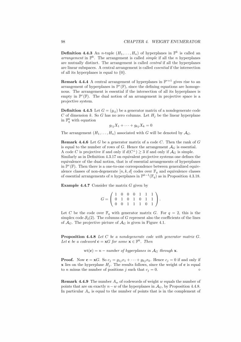
98 CHAPTER 4. WEIGHT ENUMERATOR
Definition 4.4.3 An n-tuple (H1, . . . ,Hn) of hyperplanes in Fk is called anarrangement in Fk. The arrangement is called simple if all the n hyperplanesare mutually distinct. The arrangement is called central if all the hyperplanesare linear subspaces. A central arrangement is called essential if the intersectionof all its hyperplanes is equal to 0.
Remark 4.4.4 A central arrangement of hyperplanes in Fr+1 gives rise to anarrangement of hyperplanes in Pr(F), since the defining equations are homoge-nous. The arrangement is essential if the intersection of all its hyperplanes isempty in Pr(F). The dual notion of an arrangement in projective space is aprojective system.
Definition 4.4.5 Let G = (gij) be a generator matrix of a nondegenerate codeC of dimension k. So G has no zero columns. Let Hj be the linear hyperplanein Fkq with equation
g1jX1 + · · ·+ gkjXk = 0
The arrangement (H1, . . . ,Hn) associated with G will be denoted by AG.
Remark 4.4.6 Let G be a generator matrix of a code C. Then the rank of Gis equal to the number of rows of G. Hence the arrangement AG is essential.A code C is projective if and only if d(C⊥) ≥ 3 if and only if AG is simple.Similarly as in Definition 4.3.17 on equivalent projective systems one defines theequivalence of the dual notion, that is of essential arrangements of hyperplanesin Pr(F). Then there is a one-to-one correspondence between generalized equiv-alence classes of non-degenerate [n, k, d] codes over Fq and equivalence classesof essential arrangements of n hyperplanes in Pk−1(Fq) as in Proposition 4.3.18.
Example 4.4.7 Consider the matrix G given by
G =
1 0 0 0 1 1 10 1 0 1 0 1 10 0 1 1 1 0 1
.
Let C be the code over Fq with generator matrix G. For q = 2, this is thesimplex code S2(2). The columns of G represent also the coefficients of the linesof AG. The projective picture of AG is given in Figure 4.1.
Proposition 4.4.8 Let C be a nondegenerate code with generator matrix G.Let c be a codeword c = xG for some x ∈ Fk. Then
wt(c) = n− number of hyperplanes in AG through x.
Proof. Now c = xG. So cj = g1jx1 + · · ·+ gkjxk. Hence cj = 0 if and only ifx lies on the hyperplane Hj . The results follows, since the weight of c is equalto n minus the number of positions j such that cj = 0.
Remark 4.4.9 The number Aw of codewords of weight w equals the number ofpoints that are on exactly n−w of the hyperplanes in AG, by Proposition 4.4.8.In particular An is equal to the number of points that is in the complement of
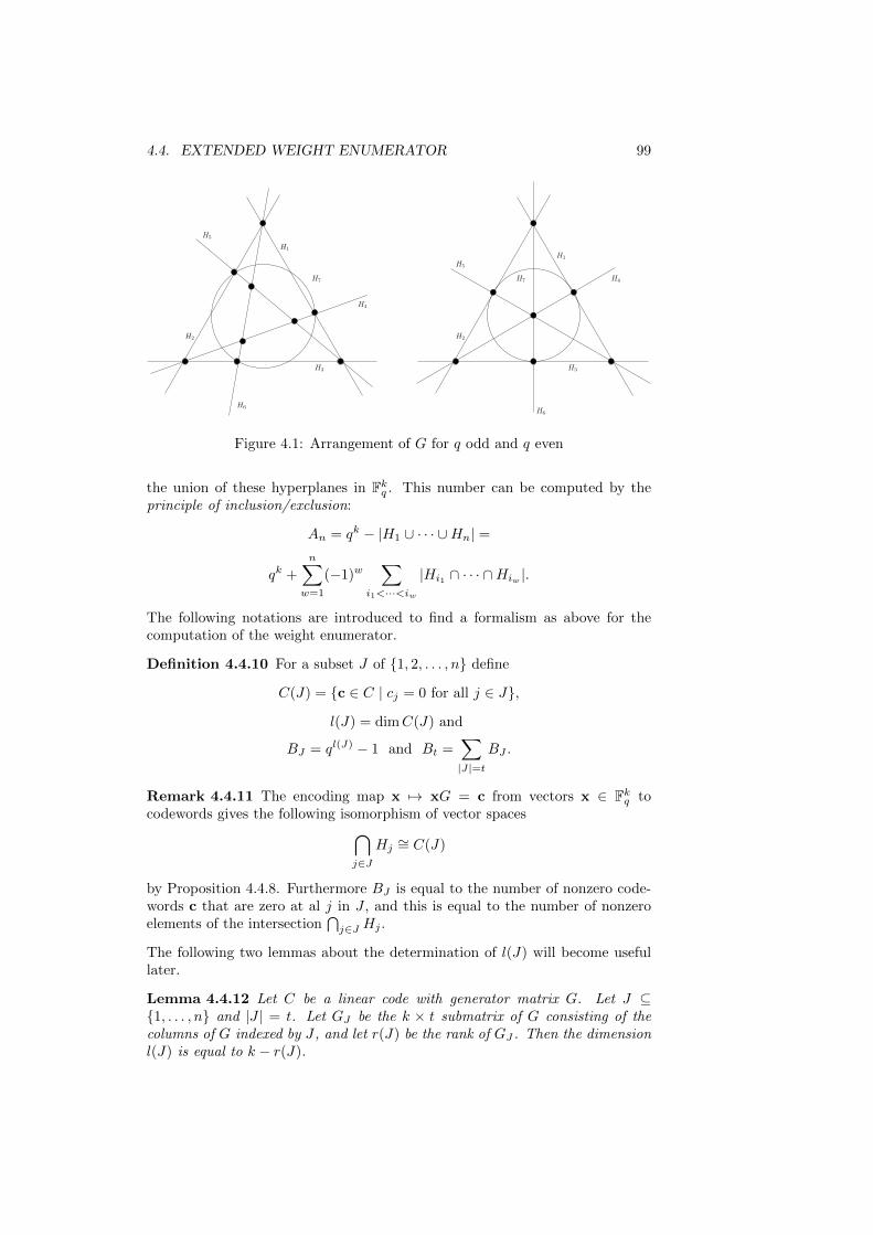
4.4. EXTENDED WEIGHT ENUMERATOR 99
H2
H4
H5
H6
H1
H4
H3
H6
H5
H7 H7
H1
H3
H2
Figure 4.1: Arrangement of G for q odd and q even
the union of these hyperplanes in Fkq . This number can be computed by theprinciple of inclusion/exclusion:
An = qk − |H1 ∪ · · · ∪Hn| =
qk +
n∑w=1
(−1)w∑
i1<···<iw
|Hi1 ∩ · · · ∩Hiw |.
The following notations are introduced to find a formalism as above for thecomputation of the weight enumerator.
Definition 4.4.10 For a subset J of 1, 2, . . . , n define
C(J) = c ∈ C | cj = 0 for all j ∈ J,
l(J) = dimC(J) and
BJ = ql(J) − 1 and Bt =∑|J|=t
BJ .
Remark 4.4.11 The encoding map x 7→ xG = c from vectors x ∈ Fkq tocodewords gives the following isomorphism of vector spaces⋂
j∈JHj∼= C(J)
by Proposition 4.4.8. Furthermore BJ is equal to the number of nonzero code-words c that are zero at al j in J , and this is equal to the number of nonzeroelements of the intersection
⋂j∈J Hj .
The following two lemmas about the determination of l(J) will become usefullater.
Lemma 4.4.12 Let C be a linear code with generator matrix G. Let J ⊆1, . . . , n and |J | = t. Let GJ be the k × t submatrix of G consisting of thecolumns of G indexed by J , and let r(J) be the rank of GJ . Then the dimensionl(J) is equal to k − r(J).
100 CHAPTER 4. WEIGHT ENUMERATOR
Proof. The code CJ is defined in 3.1.2 by restricting the codewords of C toJ . Then GJ is a generator matrix of CJ by Remark 3.1.3. Consider the theprojection map πJ : C → Fkq given by πJ(c) = cJ . Then πJ is a linear map.The image of C under πJ is CJ and the kernel of πJ is C(J) by definition. Itfollows that dimCJ + dimC(J) = dimC. So l(J) = k − r(J).
Lemma 4.4.13 Let k be the dimension of C. Let d and d⊥ be the minimumdistance the code C and its dual code, respectively. Then
l(J) =
k − t for all t < d⊥,
0 for all t > n− d.
Furthermore
k − t ≤ l(J) ≤
k − d⊥ + 1 for all t ≥ d⊥,n− d− t+ 1 for all t ≤ n− d.
Proof. (1) Let t > n − d and let J be a subset of 1, . . . , n of size t andc a codeword such that c ∈ C(J). Then J is contained in the complement ofthe support of c. Hence t ≤ n − wt(c). Hence wt(c) ≤ n − t < d. So c = 0.Therefore C(J) = 0 and l(J) = 0.(2) Let J be t-subset of 1, . . . , n. Then C(J) is defined by t homogenous linearequations on the vector space C of dimension t. So l(J) ≥ k − t.(3) The matrix G is a parity check matrix for the dual code, by (2) of Corollary2.3.29. Now suppose that t < d⊥. Then any t columns of G are independent, byProposition 2.3.11. So l(J) = k − t for all t-subsets J of 1, . . . , n by Lemma4.4.12.(4) Assume that t ≤ n − d. Let J be a t-subset. Let t′ = n − d + 1. Choose at′-subset J ′ such that J ⊆ J ′. Then
C(J ′) = c ∈ C(J) | cj = 0 for all j ∈ J ′ \ J .
Now l(J ′) = 0 by (1). Hence C(J ′) = 0 and C(J ′) is obtained from C(J)by imposing |J ′ \ J | = n − d − t + 1 linear homogeneous equations. Hencel(J) = dimC(J) ≤ n− d− t+ 1.(5) Assume that d⊥ ≤ t. Let J be a t-subset. Let t′ = d⊥ − 1. Choose at′-subset J ′ such that J ′ ⊆ J . Then l(J ′) = k− d⊥ + 1 by (3) and l(J) ≤ l(J ′),since J ′ ⊆ J . Hence l(J) ≤ k − d⊥ + 1.
Remark 4.4.14 Notice that d⊥ ≤ n − (n − k) + 1 and n − d ≤ k − 1 by theSingleton bound. So for t = k both cases of Lemma 4.4.13 apply and both givel(J) = 0.
Proposition 4.4.15 Let k be the dimension of C. Let d and d⊥ be the mini-mum distance the code C and its dual code, respectively. Then
Bt =
(nt
)(qk−t − 1) for all t < d⊥,
0 for all t > n− d.
Furthermore(n
t
)(qk−t − 1) ≤ Bt ≤
(n
t
)(qminn−d−t+1,k−d⊥+1 − 1)
for all d⊥ ≤ t ≤ n− d.
4.4. EXTENDED WEIGHT ENUMERATOR 101
Proof. This is a direct consequence of Lemma 4.4.13 and the definition of Bt.
Proposition 4.4.16 The following formula holds
Bt =
n−t∑w=d
(n− wt
)Aw.
Proof. This is shown by computing the number of elements of the set of pairs
Bt = (J, c) | J ⊆ 1, 2, . . . , n, |J | = t, c ∈ C(J), c 6= 0
in two different ways, as in Lemma 4.1.19.For fixed J , the number of these pairs is equal to BJ , by definition.If we fix the weight w of a nonzero codeword c in C, then the number of zeroentries of c is n−w and if c ∈ C(J), then J is contained in the complement ofthe support of c, and there are
(n−wt
)possible choices for such a J . In this way
we get the right hand side of the formula.
Theorem 4.4.17 The homogeneous weight enumerator of C can be expressedin terms of the Bt as follows.
WC(X,Y ) = Xn +
n∑t=0
Bt(X − Y )tY n−t.
Proof. Now
Xn +
n∑t=0
Bt(X − Y )tY n−t = Xn +
n−d∑t=0
Bt(X − Y )tY n−t,
since Bt = 0 for all t > n−d by Proposition 4.4.15. Substituting the formula forBt of Proposition 4.4.16, interchanging the order of summation in the doublesum and applying the binomial expansion of ((X − Y ) + Y )n−w gives that theabove formula is equal to
Xn +
n−d∑t=0
n−t∑w=d
(n− wt
)Aw(X − Y )tY n−t =
Xn +
n∑w=d
Aw
(n−w∑t=0
(n− wt
)(X − Y )tY n−w−t)
)Y w =
Xn +
n∑w=d
AwXn−wY w = WC(X,Y )
Proposition 4.4.18 Let A0, . . . , An be the weight spectrum of a code of mini-mum distance d. Then A0 = 1, Aw = 0 if 0 < w < d and
Aw =
n−d∑t=n−w
(−1)n+w+t
(t
n− w
)Bt if d ≤ w ≤ n.
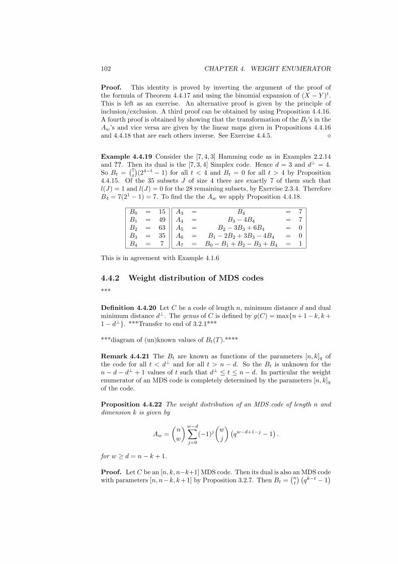
102 CHAPTER 4. WEIGHT ENUMERATOR
Proof. This identity is proved by inverting the argument of the proof ofthe formula of Theorem 4.4.17 and using the binomial expansion of (X − Y )t.This is left as an exercise. An alternative proof is given by the principle ofinclusion/exclusion. A third proof can be obtained by using Proposition 4.4.16.A fourth proof is obtained by showing that the transformation of the Bt’s in theAw’s and vice versa are given by the linear maps given in Propositions 4.4.16and 4.4.18 that are each others inverse. See Exercise 4.4.5.
Example 4.4.19 Consider the [7, 4, 3] Hamming code as in Examples 2.2.14and ??. Then its dual is the [7, 3, 4] Simplex code. Hence d = 3 and d⊥ = 4.So Bt =
(7t
)(24−t − 1) for all t < 4 and Bt = 0 for all t > 4 by Proposition
4.4.15. Of the 35 subsets J of size 4 there are exactly 7 of them such thatl(J) = 1 and l(J) = 0 for the 28 remaining subsets, by Exercise 2.3.4. ThereforeB4 = 7(21 − 1) = 7. To find the the Aw we apply Proposition 4.4.18.
B0 = 15B1 = 49B2 = 63B3 = 35B4 = 7
A3 = B4 = 7A4 = B3 − 4B4 = 7A5 = B2 − 3B3 + 6B4 = 0A6 = B1 − 2B2 + 3B3 − 4B4 = 0A7 = B0 −B1 +B2 −B3 +B4 = 1
This is in agreement with Example 4.1.6
4.4.2 Weight distribution of MDS codes
***
Definition 4.4.20 Let C be a code of length n, minimum distance d and dualminimum distance d⊥. The genus of C is defined by g(C) = maxn+ 1− k, k+1− d⊥. ***Transfer to end of 3.2.1***
***diagram of (un)known values of Bt(T ).****
Remark 4.4.21 The Bt are known as functions of the parameters [n, k]q ofthe code for all t < d⊥ and for all t > n − d. So the Bt is unknown for then − d − d⊥ + 1 values of t such that d⊥ ≤ t ≤ n − d. In particular the weightenumerator of an MDS code is completely determined by the parameters [n, k]qof the code.
Proposition 4.4.22 The weight distribution of an MDS code of length n anddimension k is given by
Aw =
(n
w
)w−d∑j=0
(−1)j(w
j
)(qw−d+1−j − 1
).
for w ≥ d = n− k + 1.
Proof. Let C be an [n, k, n−k+1] MDS code. Then its dual is also an MDS codewith parameters [n, n−k, k+1] by Proposition 3.2.7. Then Bt =
(nt
) (qk−t − 1
)
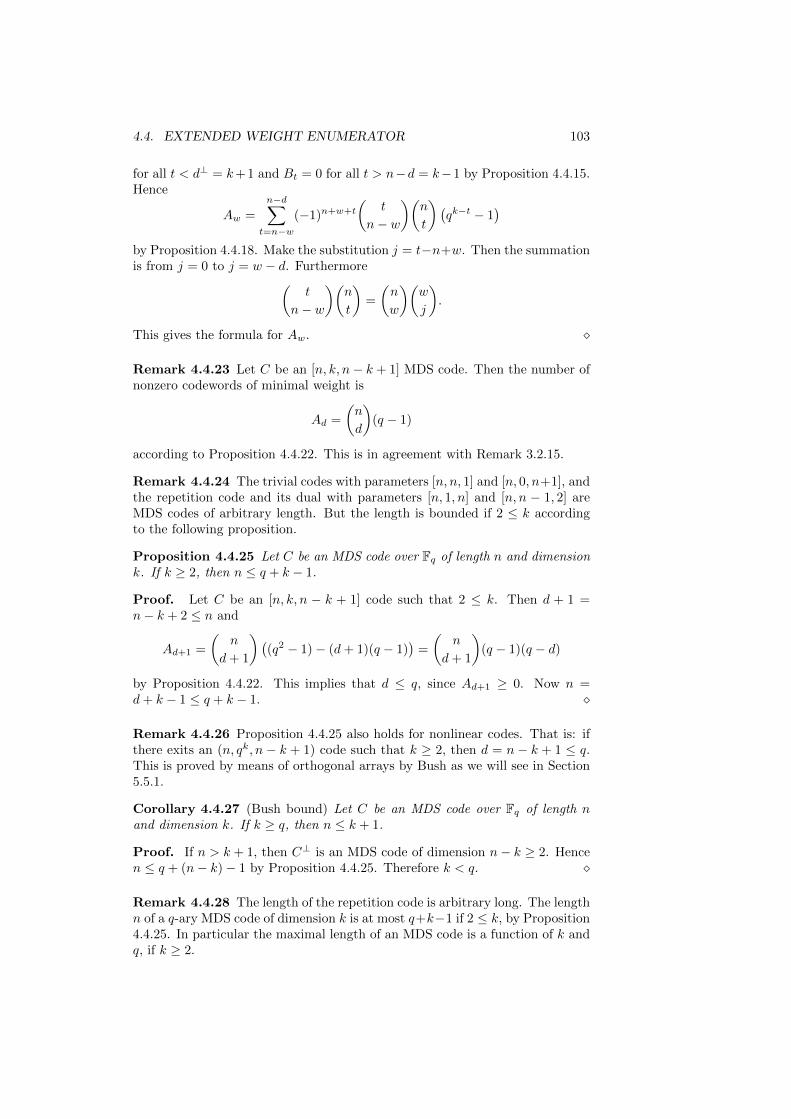
4.4. EXTENDED WEIGHT ENUMERATOR 103
for all t < d⊥ = k+1 and Bt = 0 for all t > n−d = k−1 by Proposition 4.4.15.Hence
Aw =
n−d∑t=n−w
(−1)n+w+t
(t
n− w
)(n
t
)(qk−t − 1
)by Proposition 4.4.18. Make the substitution j = t−n+w. Then the summationis from j = 0 to j = w − d. Furthermore(
t
n− w
)(n
t
)=
(n
w
)(w
j
).
This gives the formula for Aw.
Remark 4.4.23 Let C be an [n, k, n− k + 1] MDS code. Then the number ofnonzero codewords of minimal weight is
Ad =
(n
d
)(q − 1)
according to Proposition 4.4.22. This is in agreement with Remark 3.2.15.
Remark 4.4.24 The trivial codes with parameters [n, n, 1] and [n, 0, n+1], andthe repetition code and its dual with parameters [n, 1, n] and [n, n − 1, 2] areMDS codes of arbitrary length. But the length is bounded if 2 ≤ k accordingto the following proposition.
Proposition 4.4.25 Let C be an MDS code over Fq of length n and dimensionk. If k ≥ 2, then n ≤ q + k − 1.
Proof. Let C be an [n, k, n − k + 1] code such that 2 ≤ k. Then d + 1 =n− k + 2 ≤ n and
Ad+1 =
(n
d+ 1
)((q2 − 1)− (d+ 1)(q − 1)
)=
(n
d+ 1
)(q − 1)(q − d)
by Proposition 4.4.22. This implies that d ≤ q, since Ad+1 ≥ 0. Now n =d+ k − 1 ≤ q + k − 1.
Remark 4.4.26 Proposition 4.4.25 also holds for nonlinear codes. That is: ifthere exits an (n, qk, n − k + 1) code such that k ≥ 2, then d = n − k + 1 ≤ q.This is proved by means of orthogonal arrays by Bush as we will see in Section5.5.1.
Corollary 4.4.27 (Bush bound) Let C be an MDS code over Fq of length nand dimension k. If k ≥ q, then n ≤ k + 1.
Proof. If n > k + 1, then C⊥ is an MDS code of dimension n− k ≥ 2. Hencen ≤ q + (n− k)− 1 by Proposition 4.4.25. Therefore k < q.
Remark 4.4.28 The length of the repetition code is arbitrary long. The lengthn of a q-ary MDS code of dimension k is at most q+k−1 if 2 ≤ k, by Proposition4.4.25. In particular the maximal length of an MDS code is a function of k andq, if k ≥ 2.
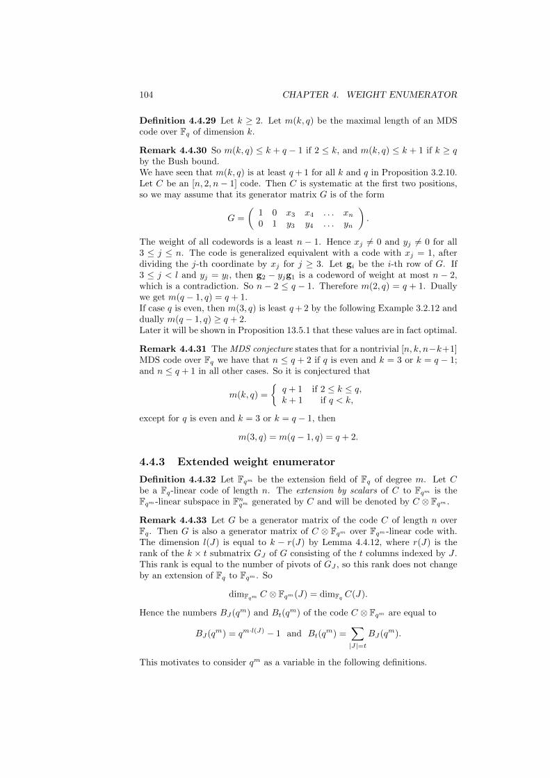
104 CHAPTER 4. WEIGHT ENUMERATOR
Definition 4.4.29 Let k ≥ 2. Let m(k, q) be the maximal length of an MDScode over Fq of dimension k.
Remark 4.4.30 So m(k, q) ≤ k + q − 1 if 2 ≤ k, and m(k, q) ≤ k + 1 if k ≥ qby the Bush bound.We have seen that m(k, q) is at least q+ 1 for all k and q in Proposition 3.2.10.Let C be an [n, 2, n− 1] code. Then C is systematic at the first two positions,so we may assume that its generator matrix G is of the form
G =
(1 0 x3 x4 . . . xn0 1 y3 y4 . . . yn
).
The weight of all codewords is a least n − 1. Hence xj 6= 0 and yj 6= 0 for all3 ≤ j ≤ n. The code is generalized equivalent with a code with xj = 1, afterdividing the j-th coordinate by xj for j ≥ 3. Let gi be the i-th row of G. If3 ≤ j < l and yj = yl, then g2 − yjg1 is a codeword of weight at most n − 2,which is a contradiction. So n − 2 ≤ q − 1. Therefore m(2, q) = q + 1. Duallywe get m(q − 1, q) = q + 1.If case q is even, then m(3, q) is least q+ 2 by the following Example 3.2.12 anddually m(q − 1, q) ≥ q + 2.Later it will be shown in Proposition 13.5.1 that these values are in fact optimal.
Remark 4.4.31 The MDS conjecture states that for a nontrivial [n, k, n−k+1]MDS code over Fq we have that n ≤ q + 2 if q is even and k = 3 or k = q − 1;and n ≤ q + 1 in all other cases. So it is conjectured that
m(k, q) =
q + 1 if 2 ≤ k ≤ q,k + 1 if q < k,
except for q is even and k = 3 or k = q − 1, then
m(3, q) = m(q − 1, q) = q + 2.
4.4.3 Extended weight enumerator
Definition 4.4.32 Let Fqm be the extension field of Fq of degree m. Let Cbe a Fq-linear code of length n. The extension by scalars of C to Fqm is theFqm-linear subspace in Fnqm generated by C and will be denoted by C ⊗ Fqm .
Remark 4.4.33 Let G be a generator matrix of the code C of length n overFq. Then G is also a generator matrix of C ⊗ Fqm over Fqm-linear code with.The dimension l(J) is equal to k − r(J) by Lemma 4.4.12, where r(J) is therank of the k × t submatrix GJ of G consisting of the t columns indexed by J .This rank is equal to the number of pivots of GJ , so this rank does not changeby an extension of Fq to Fqm . So
dimFqmC ⊗ Fqm(J) = dimFq
C(J).
Hence the numbers BJ(qm) and Bt(qm) of the code C ⊗ Fqm are equal to
BJ(qm) = qm·l(J) − 1 and Bt(qm) =
∑|J|=t
BJ(qm).
This motivates to consider qm as a variable in the following definitions.
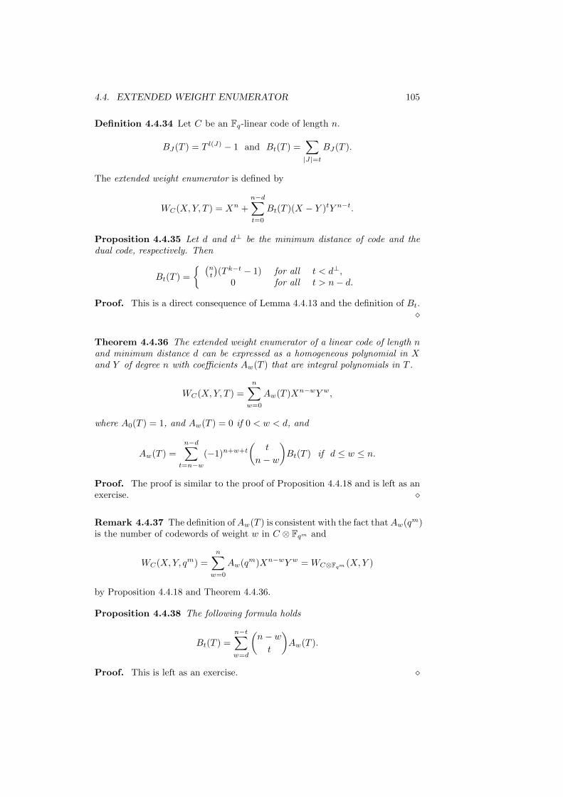
4.4. EXTENDED WEIGHT ENUMERATOR 105
Definition 4.4.34 Let C be an Fq-linear code of length n.
BJ(T ) = T l(J) − 1 and Bt(T ) =∑|J|=t
BJ(T ).
The extended weight enumerator is defined by
WC(X,Y, T ) = Xn +
n−d∑t=0
Bt(T )(X − Y )tY n−t.
Proposition 4.4.35 Let d and d⊥ be the minimum distance of code and thedual code, respectively. Then
Bt(T ) =
(nt
)(T k−t − 1) for all t < d⊥,
0 for all t > n− d.
Proof. This is a direct consequence of Lemma 4.4.13 and the definition of Bt.
Theorem 4.4.36 The extended weight enumerator of a linear code of length nand minimum distance d can be expressed as a homogeneous polynomial in Xand Y of degree n with coefficients Aw(T ) that are integral polynomials in T .
WC(X,Y, T ) =
n∑w=0
Aw(T )Xn−wY w,
where A0(T ) = 1, and Aw(T ) = 0 if 0 < w < d, and
Aw(T ) =
n−d∑t=n−w
(−1)n+w+t
(t
n− w
)Bt(T ) if d ≤ w ≤ n.
Proof. The proof is similar to the proof of Proposition 4.4.18 and is left as anexercise.
Remark 4.4.37 The definition ofAw(T ) is consistent with the fact thatAw(qm)is the number of codewords of weight w in C ⊗ Fqm and
WC(X,Y, qm) =
n∑w=0
Aw(qm)Xn−wY w = WC⊗Fqm(X,Y )
by Proposition 4.4.18 and Theorem 4.4.36.
Proposition 4.4.38 The following formula holds
Bt(T ) =
n−t∑w=d
(n− wt
)Aw(T ).
Proof. This is left as an exercise.
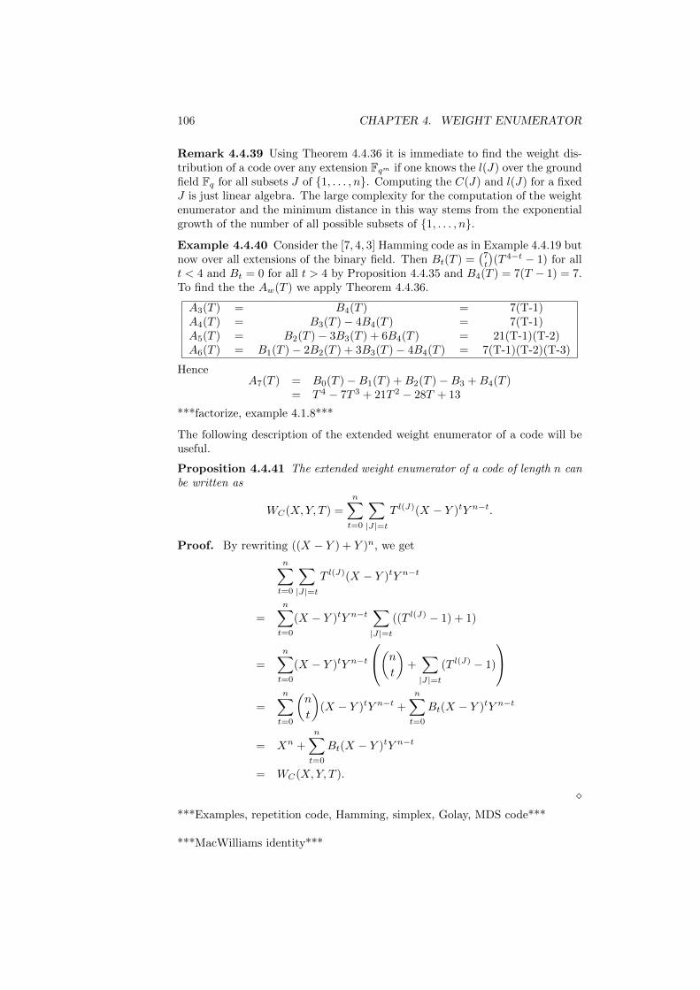
106 CHAPTER 4. WEIGHT ENUMERATOR
Remark 4.4.39 Using Theorem 4.4.36 it is immediate to find the weight dis-tribution of a code over any extension Fqm if one knows the l(J) over the groundfield Fq for all subsets J of 1, . . . , n. Computing the C(J) and l(J) for a fixedJ is just linear algebra. The large complexity for the computation of the weightenumerator and the minimum distance in this way stems from the exponentialgrowth of the number of all possible subsets of 1, . . . , n.
Example 4.4.40 Consider the [7, 4, 3] Hamming code as in Example 4.4.19 butnow over all extensions of the binary field. Then Bt(T ) =
(7t
)(T 4−t − 1) for all
t < 4 and Bt = 0 for all t > 4 by Proposition 4.4.35 and B4(T ) = 7(T − 1) = 7.To find the the Aw(T ) we apply Theorem 4.4.36.
A3(T ) = B4(T ) = 7(T-1)A4(T ) = B3(T )− 4B4(T ) = 7(T-1)A5(T ) = B2(T )− 3B3(T ) + 6B4(T ) = 21(T-1)(T-2)A6(T ) = B1(T )− 2B2(T ) + 3B3(T )− 4B4(T ) = 7(T-1)(T-2)(T-3)
HenceA7(T ) = B0(T )−B1(T ) +B2(T )−B3 +B4(T )
= T 4 − 7T 3 + 21T 2 − 28T + 13
***factorize, example 4.1.8***
The following description of the extended weight enumerator of a code will beuseful.
Proposition 4.4.41 The extended weight enumerator of a code of length n canbe written as
WC(X,Y, T ) =
n∑t=0
∑|J|=t
T l(J)(X − Y )tY n−t.
Proof. By rewriting ((X − Y ) + Y )n, we get
n∑t=0
∑|J|=t
T l(J)(X − Y )tY n−t
=
n∑t=0
(X − Y )tY n−t∑|J|=t
((T l(J) − 1) + 1)
=
n∑t=0
(X − Y )tY n−t
(nt
)+∑|J|=t
(T l(J) − 1)
=
n∑t=0
(n
t
)(X − Y )tY n−t +
n∑t=0
Bt(X − Y )tY n−t
= Xn +
n∑t=0
Bt(X − Y )tY n−t
= WC(X,Y, T ).
***Examples, repetition code, Hamming, simplex, Golay, MDS code***
***MacWilliams identity***
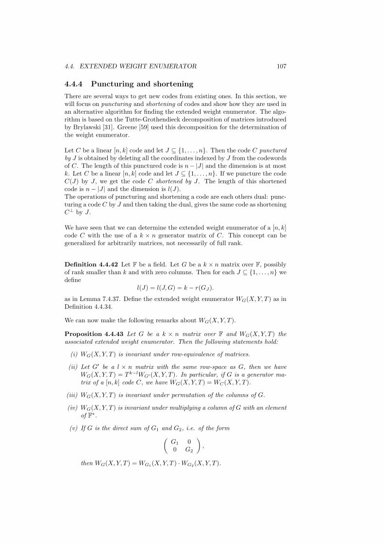
4.4. EXTENDED WEIGHT ENUMERATOR 107
4.4.4 Puncturing and shortening
There are several ways to get new codes from existing ones. In this section, wewill focus on puncturing and shortening of codes and show how they are used inan alternative algorithm for finding the extended weight enumerator. The algo-rithm is based on the Tutte-Grothendieck decomposition of matrices introducedby Brylawski [31]. Greene [59] used this decomposition for the determination ofthe weight enumerator.
Let C be a linear [n, k] code and let J ⊆ 1, . . . , n. Then the code C puncturedby J is obtained by deleting all the coordinates indexed by J from the codewordsof C. The length of this punctured code is n− |J | and the dimension is at mostk. Let C be a linear [n, k] code and let J ⊆ 1, . . . , n. If we puncture the codeC(J) by J , we get the code C shortened by J . The length of this shortenedcode is n− |J | and the dimension is l(J).The operations of puncturing and shortening a code are each others dual: punc-turing a code C by J and then taking the dual, gives the same code as shorteningC⊥ by J .
We have seen that we can determine the extended weight enumerator of a [n, k]code C with the use of a k × n generator matrix of C. This concept can begeneralized for arbitrarily matrices, not necessarily of full rank.
Definition 4.4.42 Let F be a field. Let G be a k × n matrix over F, possiblyof rank smaller than k and with zero columns. Then for each J ⊆ 1, . . . , n wedefine
l(J) = l(J,G) = k − r(GJ).
as in Lemma 7.4.37. Define the extended weight enumerator WG(X,Y, T ) as inDefinition 4.4.34.
We can now make the following remarks about WG(X,Y, T ).
Proposition 4.4.43 Let G be a k × n matrix over F and WG(X,Y, T ) theassociated extended weight enumerator. Then the following statements hold:
(i) WG(X,Y, T ) is invariant under row-equivalence of matrices.
(ii) Let G′ be a l × n matrix with the same row-space as G, then we haveWG(X,Y, T ) = T k−lWG′(X,Y, T ). In particular, if G is a generator ma-trix of a [n, k] code C, we have WG(X,Y, T ) = WC(X,Y, T ).
(iii) WG(X,Y, T ) is invariant under permutation of the columns of G.
(iv) WG(X,Y, T ) is invariant under multiplying a column of G with an elementof F∗.
(v) If G is the direct sum of G1 and G2, i.e. of the form(G1 00 G2
),
then WG(X,Y, T ) = WG1(X,Y, T ) ·WG2
(X,Y, T ).
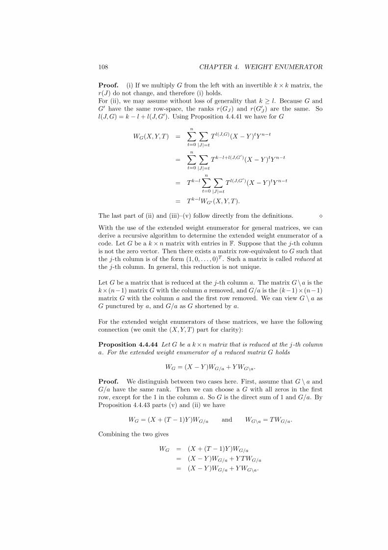
108 CHAPTER 4. WEIGHT ENUMERATOR
Proof. (i) If we multiply G from the left with an invertible k× k matrix, ther(J) do not change, and therefore (i) holds.For (ii), we may assume without loss of generality that k ≥ l. Because G andG′ have the same row-space, the ranks r(GJ) and r(G′J) are the same. Sol(J,G) = k − l + l(J,G′). Using Proposition 4.4.41 we have for G
WG(X,Y, T ) =
n∑t=0
∑|J|=t
T l(J,G)(X − Y )tY n−t
=
n∑t=0
∑|J|=t
T k−l+l(J,G′)(X − Y )tY n−t
= T k−ln∑t=0
∑|J|=t
T l(J,G′)(X − Y )tY n−t
= T k−lWG′(X,Y, T ).
The last part of (ii) and (iii)–(v) follow directly from the definitions.
With the use of the extended weight enumerator for general matrices, we canderive a recursive algorithm to determine the extended weight enumerator of acode. Let G be a k× n matrix with entries in F. Suppose that the j-th columnis not the zero vector. Then there exists a matrix row-equivalent to G such thatthe j-th column is of the form (1, 0, . . . , 0)T . Such a matrix is called reduced atthe j-th column. In general, this reduction is not unique.
Let G be a matrix that is reduced at the j-th column a. The matrix G\a is thek×(n−1) matrix G with the column a removed, and G/a is the (k−1)×(n−1)matrix G with the column a and the first row removed. We can view G \ a asG punctured by a, and G/a as G shortened by a.
For the extended weight enumerators of these matrices, we have the followingconnection (we omit the (X,Y, T ) part for clarity):
Proposition 4.4.44 Let G be a k×n matrix that is reduced at the j-th columna. For the extended weight enumerator of a reduced matrix G holds
WG = (X − Y )WG/a + YWG\a.
Proof. We distinguish between two cases here. First, assume that G \ a andG/a have the same rank. Then we can choose a G with all zeros in the firstrow, except for the 1 in the column a. So G is the direct sum of 1 and G/a. ByProposition 4.4.43 parts (v) and (ii) we have
WG = (X + (T − 1)Y )WG/a and WG\a = TWG/a.
Combining the two gives
WG = (X + (T − 1)Y )WG/a
= (X − Y )WG/a + Y TWG/a
= (X − Y )WG/a + YWG\a.
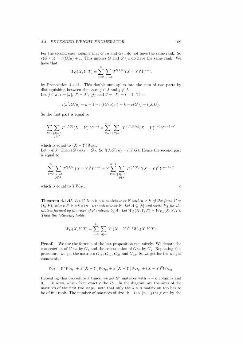
4.4. EXTENDED WEIGHT ENUMERATOR 109
For the second case, assume that G \ a and G/a do not have the same rank. Sor(G \ a) = r(G/a) + 1. This implies G and G \ a do have the same rank. Wehave that
WG(X,Y, T ) =
n∑t=0
∑|J|=t
T l(J,G)(X − Y )tY n−t.
by Proposition 4.4.41. This double sum splits into the sum of two parts bydistinguishing between the cases j ∈ J and j 6∈ J .Let j ∈ J , t = |J |, J ′ = J \ j and t′ = |J ′| = t− 1. Then
l(J ′, G/a) = k − 1− r((G/a)J′) = k − r(GJ) = l(J,G).
So the first part is equal to
n∑t=0
∑|J|=tj∈J
T l(J,G)(X − Y )tY n−t =
n−1∑t′=0
∑|J′|=t′
T l(J′,G/a)(X − Y )t
′+1Y n−1−t′
which is equal to (X − Y )WG/a.Let j 6∈ J . Then (G \ a)J = GJ . So l(J,G \ a) = l(J,G). Hence the second partis equal to
n∑t=0
∑|J|=tj 6∈J
T l(J,G)(X − Y )tY n−t = Y
n−1∑t′=0
∑|J|=t′j 6∈J
T l(J,G\a)(X − Y )t′Y n−1−t′
which is equal to YWG\a.
Theorem 4.4.45 Let G be a k × n matrix over F with n > k of the form G =(Ik|P ), where P is a k×(n−k) matrix over F. Let A ⊆ [k] and write PA for thematrix formed by the rows of P indexed by A. Let WA(X,Y, T ) = WPA
(X,Y, T ).Then the following holds:
WC(X,Y, T ) =
k∑l=0
∑|A|=l
Y l(X − Y )k−lWA(X,Y, T ).
Proof. We use the formula of the last proposition recursively. We denote theconstruction of G \ a by G1 and the construction of G/a by G2. Repeating thisprocedure, we get the matrices G11, G12, G21 and G22. So we get for the weightenumerator
WG = Y 2WG11+ Y (X − Y )WG12
+ Y (X − Y )WG21+ (X − Y )2WG22
.
Repeating this procedure k times, we get 2k matrices with n − k columns and0, . . . , k rows, which form exactly the PA. In the diagram are the sizes of thematrices of the first two steps: note that only the k × n matrix on top has tobe of full rank. The number of matrices of size (k − i)× (n− j) is given by the
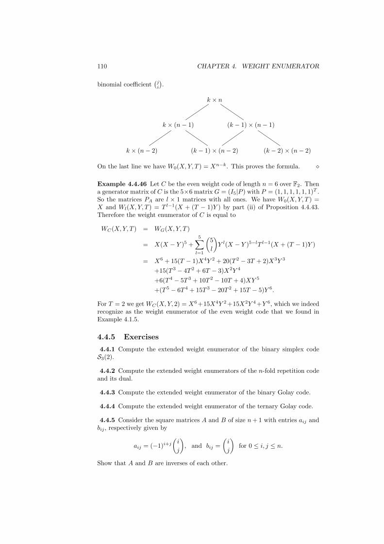
110 CHAPTER 4. WEIGHT ENUMERATOR
binomial coefficient(ji
).
k × n
k × (n− 1) (k − 1)× (n− 1)
k × (n− 2) (k − 1)× (n− 2) (k − 2)× (n− 2)
On the last line we have W0(X,Y, T ) = Xn−k. This proves the formula.
Example 4.4.46 Let C be the even weight code of length n = 6 over F2. Thena generator matrix of C is the 5×6 matrix G = (I5|P ) with P = (1, 1, 1, 1, 1, 1)T .So the matrices PA are l × 1 matrices with all ones. We have W0(X,Y, T ) =X and Wl(X,Y, T ) = T l−1(X + (T − 1)Y ) by part (ii) of Proposition 4.4.43.Therefore the weight enumerator of C is equal to
WC(X,Y, T ) = WG(X,Y, T )
= X(X − Y )5 +
5∑l=1
(5
l
)Y l(X − Y )5−lT l−1(X + (T − 1)Y )
= X6 + 15(T − 1)X4Y 2 + 20(T 2 − 3T + 2)X3Y 3
+15(T 3 − 4T 2 + 6T − 3)X2Y 4
+6(T 4 − 5T 3 + 10T 2 − 10T + 4)XY 5
+(T 5 − 6T 4 + 15T 3 − 20T 2 + 15T − 5)Y 6.
For T = 2 we get WC(X,Y, 2) = X6 +15X4Y 2 +15X2Y 4 +Y 6, which we indeedrecognize as the weight enumerator of the even weight code that we found inExample 4.1.5.
4.4.5 Exercises
4.4.1 Compute the extended weight enumerator of the binary simplex codeS3(2).
4.4.2 Compute the extended weight enumerators of the n-fold repetition codeand its dual.
4.4.3 Compute the extended weight enumerator of the binary Golay code.
4.4.4 Compute the extended weight enumerator of the ternary Golay code.
4.4.5 Consider the square matrices A and B of size n+ 1 with entries aij andbij , respectively given by
aij = (−1)i+j(i
j
), and bij =
(i
j
)for 0 ≤ i, j ≤ n.
Show that A and B are inverses of each other.
4.5. GENERALIZED WEIGHT ENUMERATOR 111
4.4.6 Give a proof of Theorem 4.4.36.
4.4.7 Give a proof of Proposition 4.4.38.
4.4.8 Compare the complexity of the methods ”exhaustive search” and ”ar-rangements of hyperplanes” to compute the weight enumerator as a function ofq and the parameters [n, k, d] and d⊥.
4.5 Generalized weight enumerator
***Intro***
4.5.1 Generalized Hamming weights
We recall that for a linear code C, the minimum Hamming weight is the min-imal one among all Hamming weights wt(c) for nonzero codewords c 6= 0. Inthis subsection, we generalize this parameter to get a sequence of values, theso-called generalized Hamming weights, which are useful in the study of thecomplexity of the trellis decoding and other properties of the code C.
***C nondegenerate?***
Let D be a subcode of C. Generalizing Definition 2.2.2, we define the supportof D, denoted by supp(D), as set of positions where at least one codeword in Dis not zero, i.e.,
supp(D) = i | there exists x ∈ D, such that xi 6= 0.
The weight of D, wt(D), is defined as the size of supp(D).
Suppose C is an [n, k] code. For any r ≤ k, the r-th generalized Hamming weight(GHW) of C is defined as
dr(C) = minwt(D) | D is a k−dimensional subcode of C.
The set of GHWs d1(C), . . . , dk(C) is called the weight hierarchy of C. Notethat since any 1−dimensional subcode has a nonzero codeword as its basis, thefirst generalized Hamming weight d1(C) is exactly equal to the minimum weightof C.
We now state several properties of generalized Hamming weights.
Proposition 4.5.1 (Monotonicity) For an [n, k] code C, the generalized Ham-ming weights satisfy
1 ≤ d1(C) < d2(C) < . . . < dk(C) ≤ n.
Proof. For any 1 ≤ r ≤ k− 1, it is trivial to verify 1 ≤ dr(C) ≤ dr+1(C) ≤ n.Let D be a subcode of dimension r+ 1, such that wt(D) = dr+1(C). We chooseany index i ∈ supp(D). Consider
E = x | x ∈ D, and xi = 0.
112 CHAPTER 4. WEIGHT ENUMERATOR
By Definition 3.1.13 and Proposition 3.1.15, E is a shortened code of D, andr ≤ dim(E) ≤ r+ 1. However, by the choice of i, there exists a codeword c ∈ Dwith ci 6= 0. Thus, c can not be a codeword of E. This implies that E is aproper subcode of D, that is dim(E) = r. Now, by the definition of the GHWs,we have
dr(C) ≤ wt(E) ≤ wt(D)− 1 = dr+1(C)− 1.
This proves that dr(C) < dr+1(C).
Proposition 4.5.2 (Generalized Singleton Bound) For an [n, k] code C, wehave
dr(C) ≤ n− k + r.
This bound on dr(C) is a straightforward consequence of the Proposition 4.5.1.When r = 1, we get the Singleton bound (see Theorem 3.2.1).
Let H be a parity check matrix of the [n, k] code C, which is a (n−k)×n matrixof rank n− k. From Proposition 2.3.11, we know that the minimum distance ofC is the smallest integer d such that d columns of H are linearly dependent. Wenow present a generalization of this property. Let Hi, 1 ≤ i ≤ n, be the columnvectors of H. For any subset I of 1, 2, . . . , n, let 〈Hi | i ∈ I〉 be the subset ofFnq generated by the vectors Hi, i ∈ I, which, for simplicity, is denoted by VI .
Lemma 4.5.3 The r-th generalized Hamming weight of C is
dr(C) = min|I| | dim(〈Hi | i ∈ I〉) ≤ |I| − r.
Proof. We denote V ⊥I = x | xi = 0 for i 6∈ I, and∑i∈I xiHi = 0. Then it
is easy to see that dim(VI) + dim(V ⊥I ) = |I|. Also, from the definition, for anyI, V ⊥I is a subcode of C.
Let D be a subcode of C with dim(D) = r and |supp(D)| = dr(C). LetI = supp(D). Then D ⊆ V ⊥I . This implies that dim(VI) = |I|−dim(V ⊥I ) ≤ |I|−dim(D) = |I| − r. Therefore, dr(C) = |supp(D)| = |I| ≥ min|I| | dim(VI) ≤|I| − r. We now prove the inverse inequality. Denote d = min|I| | dim(VI) ≤|I| − r. Let I be a subset of 1, 2, . . . , n such that dim(VI) ≤ |I| − r and|I| = d. Then dim(V ⊥I ) ≥ r. Therefore, dr(C) ≤ |supp(V ⊥I )| ≤ |I| = d.
Proposition 4.5.4 (Duality) Let C be an [n, k] code. Then the weight hierar-chy of its dual code C⊥ is completely determined by the weight hierarchy of C,precisely
dr(C⊥) | 1 ≤ r ≤ n− k = 1, 2, . . . , n\n+ 1− ds(C) | 1 ≤ s ≤ k.
Proof. Look at the two sets dr(C⊥) | 1 ≤ r ≤ n−k and n+1−ds(C) | 1 ≤s ≤ k. Both are subsets of 1, 2, . . . , n. And by the Monotonicity, the firstone has size n− k, the second one has size k. Thus, it is sufficient to prove thatthese two sets are distinct.
We now prove an equivalent fact that for any 1 ≤ r ≤ k, the value n+1−dr(C)is not a generalized Hamming weight of C⊥. Let t = n − k + r − dr(C).
4.5. GENERALIZED WEIGHT ENUMERATOR 113
It is sufficient to prove that dt(C⊥) < n + 1 − dr(C) and for any δ ≥ 1,
dt+δ(C⊥) 6= n + 1 − dr(C). Let D be a subcode of C with dim(D) = r and
|supp(D)| = dr(C). There exists a parity check matrix G for C⊥ (which is agenerator matrix for C), where the first r rows are words in D and the lastk − r rows are not. The column vectors Gi | i 6∈ supp(D) have their first rcoordinates zero. Thus, dim(〈Gi | i 6∈ supp(D)〉)= column rank of the matrix(Gi | i 6∈ supp(D)) ≤ row rank of the matrix (Ri | r + 1 ≤ i ≤ k) ≤ k − r,where Ri is the i-th row vector of G. Let I = 1, 2, . . . , n\supp(D). Then,|I| = n − dr(C). And dim(〈Gi | i ∈ I〉) ≤ k − r = |I| − t. Thus, by Lemma4.5.3, we have dt(C
⊥) ≤ |I| = n− dr(C) < n− dr(C) + 1.
Next, we show dt+δ(C⊥) 6= n+1−dr(C). Otherwise, dt+δ(C
⊥) = n+1−dr(C)holds for some δ. Then by the definition of generalized Hamming weight, thereexists a generator matrix H for C⊥ (which is a parity check matrix for C) anddr(C) − 1 positions 1 ≤ i1, . . . , idr(C)−1 ≤ n, such that the coordinates of thefirst t + δ rows of H are all zero at these dr(C) − 1 positions. Without loss ofgenerality, we assume these positions are exactly the last dr(C) − 1 positionsn − dr(C) + 2, . . . , n. And let I = n − dr(C) + 2, . . . , n. Clearly, the last |I|column vectors span a space of dimension ≤ n− k − t− δ = dr(C)− r − δ. ByLemma 4.5.3, ds(C) ≤ dr(C)−1, where s = |I|−(dr(C)−r−δ) = r+δ−1 ≥ r.This contradicts the Monotonicity.
4.5.2 Generalized weight enumerators
The weight distribution is generalized in the following way. Instead of lookingat words of C, we consider all the subcodes of C of a certain dimension r.
Definition 4.5.5 Let C be a linear code of length n. The number of subcodes
with a given weight w and dimension r is denoted by A(r)w , that is
A(r)w = |D ⊆ C|dimD = r,wt(D) = w|.
Together they form the r-th generalized weight distribution of the code. The
r-th generalized weight enumerator W(r)C (X,Y ) of C is the polynomial with the
weight distribution as coefficients, that is
W(r)C (X,Y ) =
n∑w=0
A(r)w Xn−wY w.
Remark 4.5.6 From this definition it follows that A(0)0 = 1 and A
(r)0 = 0 for
all 0 < r ≤ k. Furthermore, every 1-dimensional subspace of C contains q − 1
non-zero codewords, so (q − 1)A(1)w = Aw for 0 < w ≤ n. This means we can
find back the original weight enumerator by using
WC(X,Y ) = W(0)C (X,Y ) + (q − 1)W
(1)C (X,Y ).
Definition 4.5.7 We introduce the following notations:
[m, r]q =
r−1∏i=0
(qm − qi)
114 CHAPTER 4. WEIGHT ENUMERATOR
〈r〉q = [r, r]q[k
r
]q
=[k, r]q〈r〉q
.
Remark 4.5.8 In Proposition 2.5.2 it is shown that the first number is equalto the number of m× r matrices of rank r over Fq. and the third number is theGaussian binomial, and it represents the number of r-dimensional subspaces ofFkq . Hence the second number is the number of bases of Frq.
Definition 4.5.9 For J ⊆ 1, . . . , n and r ≥ 0 an integer we define:
B(r)J = |D ⊆ C(J)|D subspace of dimension r|
B(r)t =
∑|J|=t
B(r)J
Remark 4.5.10 Note that B(r)J =
[l(J)r
]q. For r = 0 this gives B
(0)t =
(nt
). So
we see that in general l(J) = 0 does not imply B(r)J = 0, because
[00
]q
= 1. But
if r 6= 0, we do have that l(J) = 0 implies B(r)J = 0 and B
(r)t = 0.
Proposition 4.5.11 Let dr be the r-th generalized Hamming weight of C, andd⊥ the minimum distance of the dual code C⊥. Then we have
B(r)t =
(nt
) [k−tr
]q
for all t < d⊥
0 for all t > n− dr
Proof. The first case is is a direct corollary of Lemma 4.4.13, since thereare
(nt
)subsets J ⊆ 1, . . . , n with |J | = t. The proof of the second case goes
analogous to the proof of the same lemma: let |J | = t, t > n− dr and supposethere is a subspace D ⊆ C(J) of dimension r. Then J is contained in thecomplement of supp(D), so t ≤ n−wt(D). It follows that wt(D) ≤ n− t < dr,
which is impossible, so such a D does not exist. So B(r)J = 0 for all J with
|J | = t and t > n− dr, and therefore B(r)t = 0 for t > n− dr.
We can check that the formula is well-defined: if t < d⊥ then l(J) = k − t. Ifalso t > n− dr, we have t > n− dr ≥ k− r by the generalized Singleton bound.
This implies r > k − t = l(J), so[k−tr
]q
= 0.
The relation between B(r)t and A
(r)w becomes clear in the next proposition.
Proposition 4.5.12 The following formula holds:
B(r)t =
n∑w=0
(n− wt
)A(r)w .
Proof. We will count the elements of the set
B(r)t = (D,J)|J ⊆ 1, . . . , n, |J | = t,D ⊆ C(J) subspace of dimension r
4.5. GENERALIZED WEIGHT ENUMERATOR 115
in two different ways. For each J with |J | = t there are B(r)J pairs (D,J) in
B(r)t , so the total number of elements in this set is
∑|J|=tB
(r)J = B
(r)t . On the
other hand, let D be an r-dimensional subcode of C with wt(D) = w. There are
A(r)w possibilities for such a D. If we want to find a J such that D ⊆ C(J), we
have to pick t coordinates from the n−w all-zero coordinates of D. Summationover all w proves the given formula.
Note that because A(r)w = 0 for all w < dr, we can start summation at w = dr.
We can end summation at w = n− t because for t > n−w we have(n−wt
)= 0.
So the formula can be rewritten as
B(r)t =
n−t∑w=dr
(n− wt
)A(r)w .
In practice, we will often prefer the summation given in the proposition.
Theorem 4.5.13 The generalized weight enumerator is given by the followingformula:
W(r)C (X,Y ) =
n∑t=0
B(r)t (X − Y )tY n−t.
Proof. The proof is similar to the one given for Theorem 4.4.17 and is left asan exercise.
It is possible to determine the A(r)w directly from the B
(r)t , by using the next
proposition.
Proposition 4.5.14 The following formula holds:
A(r)w =
n∑t=n−w
(−1)n+w+t
(t
n− w
)B
(r)t .
Proof. The proof is similar to the one given for Proposition 4.4.18 and is leftas an exercise.
4.5.3 Generalized weight enumerators of MDS-codes
We can use the theory in Sections 4.5.2 and 4.4.3 to calculate the weight dis-tribution, generalized weight distribution, and extended weight distribution ofa linear [n, k] code C. This is done by determining the values l(J) for eachJ ⊆ 1, . . . , n. In general, we have to look at the 2n different subcodes of Cto find the l(J), but for the special case of MDS codes we can find the weightdistributions much faster.
Proposition 4.5.15 Let C be a linear [n, k] MDS code, and let J ⊆ 1, . . . , n.Then we have
l(J) =
0 for t > k
k − t for t ≤ k
so for a given t the value of l(J) is independent of the choice of J .
116 CHAPTER 4. WEIGHT ENUMERATOR
Proof. We know that the dual of an MDS code is also MDS, so d⊥ = k + 1.Now use d = n− k + 1 in Lemma 7.4.39.
Now that we know all the l(J) for an MDS code, it is easy to find the weightdistribution.
Theorem 4.5.16 Let C be an MDS code with parameters [n, k]. Then thegeneralized weight distribution is given by
A(r)w =
(n
w
)w−d∑j=0
(−1)j(w
j
)[w − d+ 1− j
r
]q
.
The coefficients of the extended weight enumerator are given by
Aw(T ) =
(n
w
)w−d∑j=0
(−1)j(w
j
)(Tw−d+1−j − 1).
Proof. We will give the construction for the generalized weight enumeratorhere: the case of the extended weight enumerator goes similar and is left as an
exercise. We know from Proposition 4.5.15 that for an MDS code, B(r)t depends
only on the size of J , so B(r)t =
(nt
) [k−tr
]q. Using this in the formula for A
(r)w
and substituting j = t− n+ w, we have
A(r)w =
n−dr∑t=n−w
(−1)n+w+t
(t
n− w
)B
(r)t
=
n−dr∑t=n−w
(−1)t−n+w
(t
n− w
)(n
t
)[k − tr
]q
=
w−dr∑j=0
(−1)j(n
w
)(w
j
)[k + w − n− j
r
]q
=
(n
w
)w−dr∑j=0
(−1)j(w
j
)[w − d+ 1− j
r
]q
.
In the second step, we are using the binomial equivalence(n
t
)(t
n− w
)=
(n
n− w
)(n− (n− w)
t− (n− w)
)=
(n
w
)(w
n− t
).
So, for all MDS-codes with given parameters [n, k] the extended and generalizedweight distributions are the same. But not all such codes are equivalent. Wecan conclude from this, that the generalized and extended weight enumeratorsare not enough to distinguish between codes with the same parameters. Weillustrate the non-equivalence of two MDS codes by an example.
4.5. GENERALIZED WEIGHT ENUMERATOR 117
Example 4.5.17 Let C be a linear [n, 3] MDS code over Fq. It is possible towrite the generator matrix G of C in the following form: 1 1 . . . 1
x1 x2 . . . xny1 y2 . . . yn
.
Because C is MDS we have d = n − 2. We now view the n columns of G aspoints in the projective plane P2(Fq), say P1, . . . , Pn. The MDS property thatevery k columns of G are independent is now equivalent with saying that nothree points are on a line. To see that these n points do not always determinean equivalent code, consider the following construction. Through the n pointsthere are
(n2
)= N lines, the set N . These lines determine (the generator ma-
trix of) a [N, 3] code C. The minimum distance of the code C is equal to thetotal number of lines minus the maximum number of lines from N through anarbitrarily point P ∈ P2(Fq) by Proposition 4.4.8. If P /∈ P1, . . . , Pn thenthe maximum number of lines from N through P is at most 1
2n, since no threepoints of N lie on a line. If P = Pi for some i ∈ 1, . . . , n then P lies on ex-actly n− 1 lines of N , namely the lines PiPj for j 6= i. Therefore the minimum
distance of C is d = N − n+ 1.
We now have constructed a [N, 3, N − n+ 1] code C from the original code C.Notice that two codes C1 and C2 are generalized equivalent if C1 and C2 aregeneralized equivalent. The generalized and extended weight enumerators of anMDS code of length n and dimension k are completely determined by the pair(n, k), but this is not generally true for the weight enumerator of C.
Take for example n = 6 and q = 9, so C is a [15, 3, 10] code. Look at the codesC1 and C2 generated by the following matrices respectively, where α ∈ F9 is aprimitive element: 1 1 1 1 1 1
0 1 0 1 α5 α6
0 0 1 α3 α α3
1 1 1 1 1 10 1 0 α7 α4 α6
0 0 1 α5 α 1
Being both MDS codes, the weight distribution is (1, 0, 0, 120, 240, 368). If wenow apply the above construction, we get C1 and C2 generated by 1 0 0 1 1 α4 α6 α3 α7 α 1 α2 1 α7 1
0 1 0 α7 1 0 0 α4 1 1 0 α6 α 1 α3
0 0 1 1 0 1 1 1 0 0 1 1 1 1 1
1 0 0 α7 α2 α3 α 0 α7 α7 α4 α7 α 0 0
0 1 0 1 0 α3 0 α6 α6 0 α7 α α6 α3 α0 0 1 α5 α5 α6 α3 α7 α4 α3 α5 α2 α4 α α5
The weight distribution of C1 and C2 are, respectively,
(1, 0, 0, 0, 0, 0, 0, 0, 0, 0, 48, 0, 16, 312, 288, 64) and(1, 0, 0, 0, 0, 0, 0, 0, 0, 0, 48, 0, 32, 264, 336, 48).
So the latter two codes are not generalized equivalent, and therefore not all[6, 3, 4] MDS codes over F9 are generalized equivalent.
118 CHAPTER 4. WEIGHT ENUMERATOR
Another example was given in [110, 29] showing that two [6, 3, 4] MDS codescould have distinct covering radii.
4.5.4 Connections
There is a connection between the extended weight enumerator and the gener-alized weight enumerators. We first proof the next proposition.
Proposition 4.5.18 Let C be a linear [n, k] code over Fq, and let Cm be thelinear subspace consisting of the m × n matrices over Fq whose rows are in C.Then there is an isomorphism of Fq-vector spaces between C ⊗ Fqm and Cm.
Proof. Let α be a primitive m-th root of unity in Fqm . Then we canwrite an element of Fqm in an unique way on the basis (1, α, α2, . . . , αm−1) withcoefficients in Fq. If we do this for all the coordinates of a word in C ⊗ Fqm , weget an m× n matrix over Fq. The rows of this matrix are words of C, becauseC and C ⊗ Fqm have the same generator matrix. This map is clearly injective.There are (qm)k = qkm words in C ⊗ Fqm , and the number of elements of Cm
is (qk)m = qkm, so our map is a bijection. It is given by(m−1∑i=0
ci1αi,
m−1∑i=0
ci2αi, . . . ,
m−1∑i=0
cinαi
)7→
c01 c02 c03 . . . c0nc11 c12 c13 . . . c1n...
......
. . ....
c(m−1)1 c(m−1)2 c(m−1)3 . . . c(m−1)n
.
We see that the map is Fq-linear, so it gives an isomorphism C ⊗Fqm → Cm.
Note that this isomorphism depends on the choice of a primitive element α. Wealso need the next subresult.
Lemma 4.5.19 Let c ∈ C⊗Fqm and M ∈ Cm the corresponding m×n matrixunder a given isomorphism. Let D ⊆ C be the subcode generated by the rows ofM . Then wt(c) = wt(D).
Proof. If the j-th coordinate cj of c is zero, then the j-th column of M consistsof only zero’s, because the representation of cj on the basis (1, α, α2, . . . , αm−1)is unique. On the other hand, if the j-th column of M consists of all zeros, thencj is also zero. Therefore wt(c) = wt(D).
Proposition 4.5.20 Let C be a linear code over Fq. Then the weight numera-tor of an extension code and the generalized weight enumerators are connectedvia
Aw(qm) =
m∑r=0
[m, r]qA(r)w .
Proof. We count the number of words in C ⊗ Fqm of weight w in two ways,using the bijection of Proposition 4.5.18. The first way is just by substitutingT = qm in Aw(T ): this gives the left side of the equation. For the second way,
4.5. GENERALIZED WEIGHT ENUMERATOR 119
note that every M ∈ Cm generates a subcode of C whose weight is equal tothe weight of the corresponding word in C ⊗ Fqm . Fix this weight w and a
dimension r: there are A(r)w subcodes of C of dimension r and weight w. Every
such subcode is generated by an r × n matrix whose rows are words of C. Leftmultiplication by an m × r matrix of rank r gives an element of Cm whichgenerates the same subcode of C, and all such elements of Cm are obtained thisway. The number of m× r matrices of rank r is [m, r]q, so summation over alldimensions r gives
Aw(qm) =
k∑r=0
[m, r]qA(r)w .
We can let the summation run to m, because A(r)w = 0 for r > k and [m, r]q = 0
for r > m. This proves the given formula.
In general, we have the following theorem.
Theorem 4.5.21 Let C be a linear code over Fq. Then the extended weightnumerator is determined by the generalized weight enumerators:
WC(X,Y, T ) =
k∑r=0
r−1∏j=0
(T − qj)
W(r)C (X,Y ).
Proof. If we know A(r)w for all r, we can determine Aw(qm) for every m. If
we have k + 1 values of m for which Aw(qm) is known, we can use Lagrangeinterpolation to find Aw(T ), for this is a polynomial in T of degree at most k.In fact, we have
Aw(T ) =
k∑r=0
r−1∏j=0
(T − qj)
A(r)w .
This formula has the right degree and is correct for T = qm for all integer valuesm ≥ 0, so we know it must be the correct polynomial. Therefore the theoremfollows.
The converse of the theorem is also true: we can write the generalized weightenumerator in terms of the extended weight enumerator. For this end the fol-lowing lemma is needed.
Lemma 4.5.22
r−1∏j=0
(Z − qj) =
r∑j=0
[r
j
]q
(−1)r−jq(r−j
2 )Zj .
Proof. This identity can be proven by induction and is left as an exercise.
Theorem 4.5.23 Let C be a linear code over Fq. Then the r-th generalizedweight enumerator is determined by the extended weight enumerator:
W(r)C (X,Y ) =
1
〈r〉q
r∑j=0
[r
j
]q
(−1)r−jq(r−j
2 ) WC(X,Y, qj).
120 CHAPTER 4. WEIGHT ENUMERATOR
Proof. We consider the generalized weight enumerator in terms of Theorem4.5.13. Using Remark ?? and rewriting gives the following:
W(r)C (X,Y ) =
n∑t=0
B(r)t (X − Y )tY n−t
=
n∑t=0
∑|J|=t
[l(J)
r
]q
(X − Y )tY n−t
=
n∑t=0
∑|J|=t
r−1∏j=0
ql(J) − qj
qr − qj
(X − Y )tY n−t
=1∏r−1
v=0(qr − qv)
n∑t=0
∑|J|=t
r−1∏j=0
(ql(J) − qj)
(X − Y )tY n−t
=1
〈r〉q
n∑t=0
∑|J|=t
r∑j=0
[r
j
]q
(−1)r−jq(r−j
2 )qj·l(J)(X − Y )tY n−t
=1
〈r〉q
r∑j=0
[r
j
]q
(−1)r−jq(r−j
2 )n∑t=0
∑|J|=t
(qj)l(J)(X − Y )tY n−t
=1
〈r〉q
r∑j=0
[r
j
]q
(−1)r−jq(r−j
2 ) WC(X,Y, qj)
In the fourth step Lemma 4.5.22 is used.
4.5.5 Exercises
4.5.1 Give a proof of Proposition 4.5.16.
4.5.2 Compute the generalized weight enumerator of the binary Golay code.
4.5.3 Compute the generalized weight enumerator of the ternary Golay code.
4.5.4 Give a proof of Lemma 4.5.22.
4.6 Notes
Puncturing and shortening at arbitrary sets of positions and the duality theo-rem is from Simonis [?].
Golay code, Turyn [?] construction, Pless handbook [?] .
MacWillimas
***–puncturing gives the binary [23,12,7] Golay code, which is cyclic.–automorphism group of (extended) Golay code.– (ext4ended) ternary Golay code.
4.6. NOTES 121
– designs and Golay codes.– lattices and Golay codes.***
***repeated decoding of product code (Hoeholdt-Justesen).
***Singleton defect s(C) = n+ 1− k − ds(C) ≥ 0 and equality holds if and only if C is MDS.s(C) = 0 if and only if s(C⊥) = 0.Example where s(C) = 1 and s(C⊥) > 1.Almost MDS and near MDS.Genus g = maxs(C), s(C⊥) in 4.1. If k ≥ 2, then d ≤ q(s+ 1). If k ≥ 3 andd = q(s+ 1), then s+ 1 ≤ q.Faldum-Willems, de Boer, Dodunekov-Langev,relation with Griesmer bound******Incidence structures and geometric codes

122 CHAPTER 4. WEIGHT ENUMERATOR
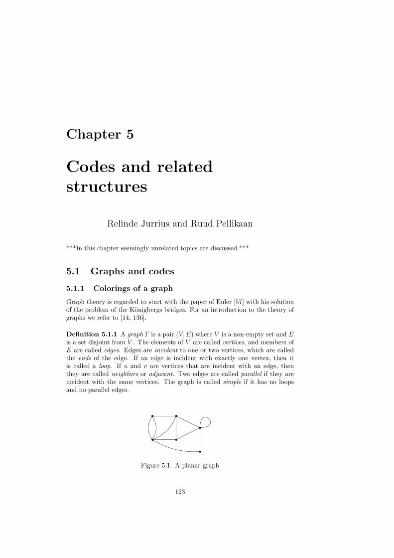
Chapter 5
Codes and relatedstructures
Relinde Jurrius and Ruud Pellikaan
***In this chapter seemingly unrelated topics are discussed.***
5.1 Graphs and codes
5.1.1 Colorings of a graph
Graph theory is regarded to start with the paper of Euler [57] with his solutionof the problem of the Konigbergs bridges. For an introduction to the theory ofgraphs we refer to [14, 136].
Definition 5.1.1 A graph Γ is a pair (V,E) where V is a non-empty set and Eis a set disjoint from V . The elements of V are called vertices, and members ofE are called edges. Edges are incident to one or two vertices, which are calledthe ends of the edge. If an edge is incident with exactly one vertex, then itis called a loop. If u and v are vertices that are incident with an edge, thenthey are called neighbors or adjacent. Two edges are called parallel if they areincident with the same vertices. The graph is called simple if it has no loopsand no parallel edges.
•
•
•
•
•
•
Figure 5.1: A planar graph
123
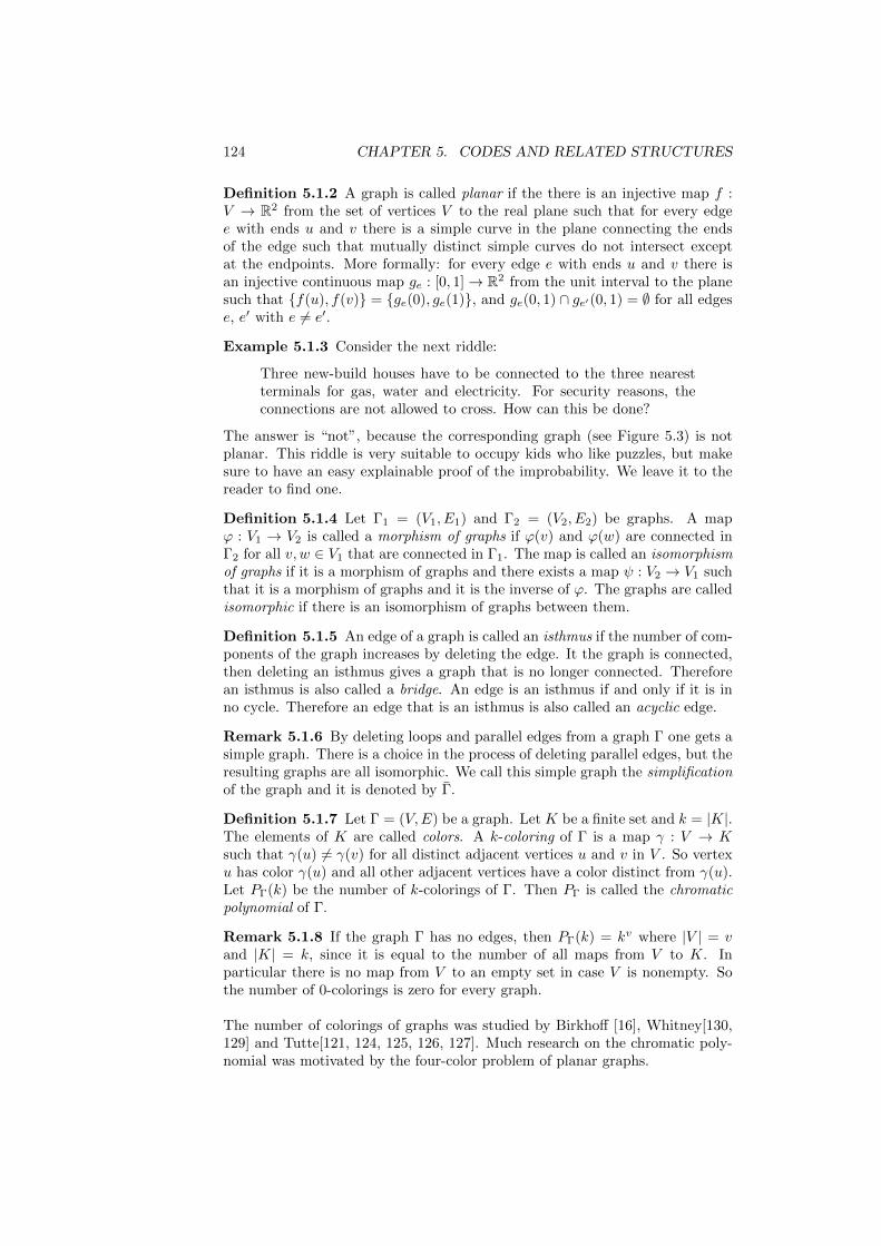
124 CHAPTER 5. CODES AND RELATED STRUCTURES
Definition 5.1.2 A graph is called planar if the there is an injective map f :V → R2 from the set of vertices V to the real plane such that for every edgee with ends u and v there is a simple curve in the plane connecting the endsof the edge such that mutually distinct simple curves do not intersect exceptat the endpoints. More formally: for every edge e with ends u and v there isan injective continuous map ge : [0, 1]→ R2 from the unit interval to the planesuch that f(u), f(v) = ge(0), ge(1), and ge(0, 1) ∩ ge′(0, 1) = ∅ for all edgese, e′ with e 6= e′.
Example 5.1.3 Consider the next riddle:
Three new-build houses have to be connected to the three nearestterminals for gas, water and electricity. For security reasons, theconnections are not allowed to cross. How can this be done?
The answer is “not”, because the corresponding graph (see Figure 5.3) is notplanar. This riddle is very suitable to occupy kids who like puzzles, but makesure to have an easy explainable proof of the improbability. We leave it to thereader to find one.
Definition 5.1.4 Let Γ1 = (V1, E1) and Γ2 = (V2, E2) be graphs. A mapϕ : V1 → V2 is called a morphism of graphs if ϕ(v) and ϕ(w) are connected inΓ2 for all v, w ∈ V1 that are connected in Γ1. The map is called an isomorphismof graphs if it is a morphism of graphs and there exists a map ψ : V2 → V1 suchthat it is a morphism of graphs and it is the inverse of ϕ. The graphs are calledisomorphic if there is an isomorphism of graphs between them.
Definition 5.1.5 An edge of a graph is called an isthmus if the number of com-ponents of the graph increases by deleting the edge. It the graph is connected,then deleting an isthmus gives a graph that is no longer connected. Thereforean isthmus is also called a bridge. An edge is an isthmus if and only if it is inno cycle. Therefore an edge that is an isthmus is also called an acyclic edge.
Remark 5.1.6 By deleting loops and parallel edges from a graph Γ one gets asimple graph. There is a choice in the process of deleting parallel edges, but theresulting graphs are all isomorphic. We call this simple graph the simplificationof the graph and it is denoted by Γ.
Definition 5.1.7 Let Γ = (V,E) be a graph. Let K be a finite set and k = |K|.The elements of K are called colors. A k-coloring of Γ is a map γ : V → Ksuch that γ(u) 6= γ(v) for all distinct adjacent vertices u and v in V . So vertexu has color γ(u) and all other adjacent vertices have a color distinct from γ(u).Let PΓ(k) be the number of k-colorings of Γ. Then PΓ is called the chromaticpolynomial of Γ.
Remark 5.1.8 If the graph Γ has no edges, then PΓ(k) = kv where |V | = vand |K| = k, since it is equal to the number of all maps from V to K. Inparticular there is no map from V to an empty set in case V is nonempty. Sothe number of 0-colorings is zero for every graph.
The number of colorings of graphs was studied by Birkhoff [16], Whitney[130,129] and Tutte[121, 124, 125, 126, 127]. Much research on the chromatic poly-nomial was motivated by the four-color problem of planar graphs.
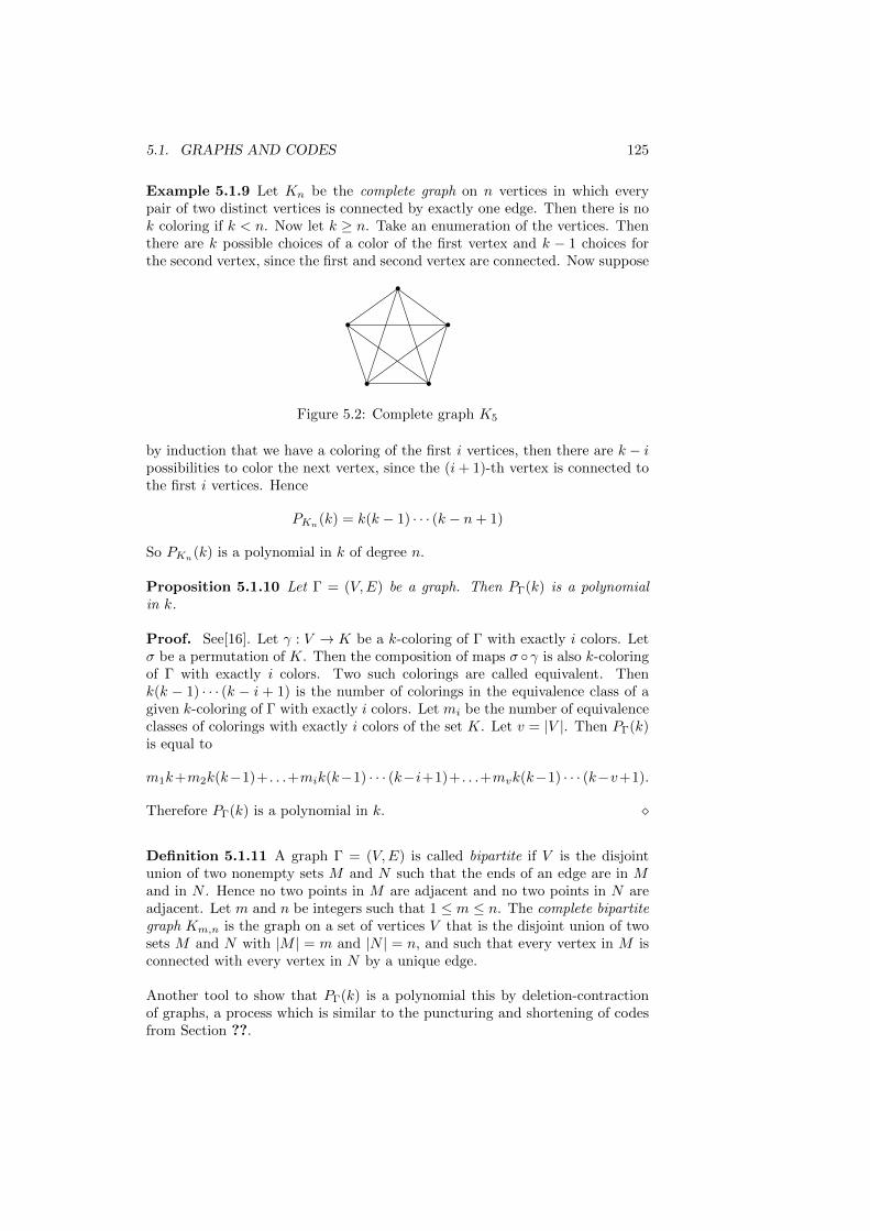
5.1. GRAPHS AND CODES 125
Example 5.1.9 Let Kn be the complete graph on n vertices in which everypair of two distinct vertices is connected by exactly one edge. Then there is nok coloring if k < n. Now let k ≥ n. Take an enumeration of the vertices. Thenthere are k possible choices of a color of the first vertex and k − 1 choices forthe second vertex, since the first and second vertex are connected. Now suppose
•
•
•
• •
Figure 5.2: Complete graph K5
by induction that we have a coloring of the first i vertices, then there are k − ipossibilities to color the next vertex, since the (i+ 1)-th vertex is connected tothe first i vertices. Hence
PKn(k) = k(k − 1) · · · (k − n+ 1)
So PKn(k) is a polynomial in k of degree n.
Proposition 5.1.10 Let Γ = (V,E) be a graph. Then PΓ(k) is a polynomialin k.
Proof. See[16]. Let γ : V → K be a k-coloring of Γ with exactly i colors. Letσ be a permutation of K. Then the composition of maps σ γ is also k-coloringof Γ with exactly i colors. Two such colorings are called equivalent. Thenk(k − 1) · · · (k − i + 1) is the number of colorings in the equivalence class of agiven k-coloring of Γ with exactly i colors. Let mi be the number of equivalenceclasses of colorings with exactly i colors of the set K. Let v = |V |. Then PΓ(k)is equal to
m1k+m2k(k−1)+ . . .+mik(k−1) · · · (k−i+1)+ . . .+mvk(k−1) · · · (k−v+1).
Therefore PΓ(k) is a polynomial in k.
Definition 5.1.11 A graph Γ = (V,E) is called bipartite if V is the disjointunion of two nonempty sets M and N such that the ends of an edge are in Mand in N . Hence no two points in M are adjacent and no two points in N areadjacent. Let m and n be integers such that 1 ≤ m ≤ n. The complete bipartitegraph Km,n is the graph on a set of vertices V that is the disjoint union of twosets M and N with |M | = m and |N | = n, and such that every vertex in M isconnected with every vertex in N by a unique edge.
Another tool to show that PΓ(k) is a polynomial this by deletion-contractionof graphs, a process which is similar to the puncturing and shortening of codesfrom Section ??.
126 CHAPTER 5. CODES AND RELATED STRUCTURES
•
• • •
• •
Figure 5.3: Complete bipartite graph K3,3
Definition 5.1.12 Let Γ = (V,E) be a graph. Let e be an edge that is incidentto the vertices u and v. Then the deletion Γ\e is the graph with vertices V andedges E \ e. The contraction Γ/e is the graph obtained by identifying u andv and deleting e. Formally this is defined as follows. Let u = v = u, v, andw = w if w 6= u and w 6= v. Let V = w : w ∈ V . Then Γ/e is the graph(V , E \ e), where an edge f 6= e is incident with w in Γ/e if f is incident withw in Γ.
Remark 5.1.13 Notice that the number of k-colorings of Γ does not changeby deleting loops and a parallel edge. Hence the chromatic polynomial Γ andits simplification Γ are the same.
The following proposition is due to Foster. See the concluding note in [129].
Proposition 5.1.14 Let Γ = (V,E) be a simple graph. Let e be an edge of Γ.Then the following deletion-contraction formula holds:
PΓ(k) = PΓ\e(k)− PΓ/e(k)
for all positive integers k.
Proof. Let u and v be the vertices of e. Then u 6= v, since the graph issimple. Let γ be a k-coloring of Γ \ e. Then γ is also a coloring of Γ if andonly if γ(u) 6= γ(v). If γ(u) = γ(v), then consider the induced map γ on Vdefined by γ(u) = γ(u) and γ(w) = γ(w) if w 6= u and w 6= v. The map γ givesa k-coloring of Γ/e. Conversely, every k-coloring of Γ/e gives a k-coloring γ ofΓ \ e such that γ(v) = γ(w). Therefore
PΓ\e(k) = PΓ(k) + PΓ/e(k).
This follows also from a more general deletion-contraction formula for matroidsthat will be treated in Section 5.2.6 and Proposition ??.
5.1.2 Codes on graphs
Definition 5.1.15 Let Γ = (V,E) be a graph. Suppose that V ′ ⊆ V andE′ ⊆ E and all the endpoints of e′ in E′ are in V ′. Then Γ′ = (V ′, E′) is agraph and it is called a subgraph of Γ.
Definition 5.1.16 Two vertices u to v are connected by a path from u to vif there is a t-tuple of mutually distinct vertices (v1, . . . , vt) with u = v1 andv = vt, and a (t− 1)-tuple of mutually distinct edges (e1, . . . , et−1) such that eiis incident with vi and vi+1 for all 1 ≤ i < t. If moreover et is an edge that isincident with u and v and distinct from ei for all i < t, then (e1, . . . , et−1, et) iscalled a cycle. The length of the smallest cycle is called the girth of the graphand is denoted by γ(Γ).
5.1. GRAPHS AND CODES 127
Definition 5.1.17 The graph is called connected if every two vertices are con-nected by a path. A maximal connected subgraph of Γ is called a connectedcomponent of Γ. The vertex set V of Γ is a disjoint union of subsets Vi and setof edges E is a disjoint union of subsets Ei such that Γi = (Vi, Ei) is a connectedcomponent of Γ. The number of connected components of Γ is denoted by c(Γ).
Definition 5.1.18 Let Γ = (V,E) be a finite graph. Suppose that V consistsof m elements enumerated by v1, . . . , vm. Suppose that E consists of n elementsenumerated by e1, . . . , en. The incidence matrix I(Γ) is a m × n matrix withentries aij defined by
aij =
1 if ej is incident with vi and vk for some i < k,−1 if ej is incident with vi and vk for some i > k,0 otherwise.
Suppose moreover that Γ is simple. Then AΓ is the arrangement (H1, . . . ,Hn)of hyperplanes where Hj = Xi −Xk if ej is incident with vi and vk with i < k.An arrangement A is called graphic if A is isomorphic with AΓ for some graphΓ.
***characteristic polynomial det(A− λI), Matrix tree theorem
Definition 5.1.19 The graph code of Γ over Fq is the Fq-linear code that isgenerated by the rows of the incidence matrix I(Γ). The cycle code CΓ of Γ isthe dual of the graph code of Γ.
Remark 5.1.20 Let Γ be a finite graph without loops. Then the arrangementAΓ is isomorphic with ACΓ
.
Proposition 5.1.21 Let Γ be a finite graph. Then CΓ is a code with parameters[n, k, d], where n = |E|, k = |E| − |V |+ c(Γ) and d = γ(Γ).
Proof. See [14, Prop. 4.3]
***Sparse graph codes, Gallager or Low-density parity check codes and Tannergraph codes play an important role in the research of coding theory at this mo-ment. See [77, 99].
5.1.3 Exercises
5.1.1 Determine the chromatic polynomial of the bipartite graph K3,2.
5.1.2 Determine the parameters of the cycle code of the complete graph Km.Show that the code CK4
over F2 is equivalent to the punctured binary [7, 3, 4]simplex code.
5.1.3 Determine the parameters of the cycle code of the bipartite graph Km,n.Let C(m) be the dual of the n-fold repetition code. Show that CKm,n is equiv-alent to the product code C(m)⊗ C(n).
128 CHAPTER 5. CODES AND RELATED STRUCTURES
5.2 Matroids and codes
Matroids were introduced by Whitney [130, 131] in axiomatizing and generaliz-ing the concepts of independence in linear algebra and circuit in graph theory.In the theory of arrangements one uses the notion of a geometric lattice. Ingraph and coding theory one refers more to matroids.
5.2.1 Matroids
Definition 5.2.1 A matroid M is a pair (E, I) consisting of a finite set E anda collection I of subsets of E such that the following three conditions hold.
(I.1) ∅ ∈ I.
(I.2) If J ⊆ I and I ∈ I, then J ∈ I.
(I.3) If I, J ∈ I and |I| < |J |, then there exists a j ∈ (J\I) such that I∪j ∈ I.
A subset I of E is called independent if I ∈ I , otherwise it is called dependent.Condition (I.2) is called the independence augmentation axiom.
Remark 5.2.2 If J is a subset of E, then J has a maximal independent subset,that is there exists an I ∈ I such that I ⊆ J and I is maximal with respect tothis property and the inclusion. If I1 and I2 are maximal independent subsetsof J , then |I1| = |I2| by condition (I.3). The rank or dimension of a subsetJ of E is the number of elements of a maximal independent subset of J . Anindependent set of rank r(M) is called a basis of M . The collection of all basesof M is denoted by B.
Example 5.2.3 Let n and k be non-negative integers such that k ≤ n. LetUn,k be a set consisting of n elements and In,k = I ⊆ Un,k||I| ≤ k. Then(Un,k, In,k) is a matroid and called the uniform matroid of rank k on n elements.A subset B of Un,k is a basis if and only if |B| = k. The matroid Un,n has nodependent sets and is called free.
Definition 5.2.4 Let (E, I) be a matroid. An element x in E is called a loop ifx is a dependent set. Let x and y in E be two distinct elements that are notloops. Then x and y are called parallel if r(x, y) = 1. The matroid is calledsimple if it has no loops and no parallel elements. Now Un,r is the only simplematroid of rank r if r ≤ 2.
Remark 5.2.5 LetG be a k×nmatrix with entries in a field F. Let E be the set[n] indexing the columns of G and IG be the collection of all subsets I of E suchthat the submatrix GI consisting of the columns of G at the positions of I areindependent. Then MG = (E, IG) is a matroid. Suppose that F is a finite fieldand G1 and G2 are generator matrices of a code C, then (E, IG1
) = (E, IG2).
So the matroid MC = (E, IC) of a code C is well defined by (E, IG) for somegenerator matrix G of C. If C is degenerate, then there is a position i such thatci = 0 for every codeword c ∈ C and all such positions correspond one-to-onewith loops of MC . Let C be nondegenerate. Then MC has no loops, and thepositions i and j with i 6= j are parallel in MC if and only if the i-th column ofG is a scalar multiple of the j-th column. The code C is projective if and only ifthe arrangement AG is simple if and only if the matroid MC is simple. A [n, k]code C is MDS if and only if the matroid MC is the uniform matroid Un,k.
5.2. MATROIDS AND CODES 129
Definition 5.2.6 Let M = (E, I) be a matroid. Let B be the collection of allbases of M . Define B⊥ = (E \ B) for B ∈ B, and B⊥ = B⊥ : B ∈ B. DefineI⊥ = I ⊆ E : I ⊆ B for some B ∈ B⊥. Then (E, I⊥) is called the dualmatroid of M and is denoted by M⊥.
Remark 5.2.7 The dual matroid is indeed a matroid. Let C be a code over afinite field. Then (MC)⊥ is isomorphic with MC⊥ as matroids.
Let e be a loop of the matroid M . Then e is not a member of any basis of M .Hence e is in every basis of M⊥. An element of M is called an isthmus if it isan element of every basis of M . Hence e is an isthmus of M if and only if e isa loop of M⊥.
Proposition 5.2.8 Let (E, I) be a matroid with rank function r. Then thedual matroid has rank function r⊥ given by
r⊥(J) = |J | − r(E) + r(E \ J).
Proof. The proof is based on the observation that r(J) = maxB∈B |B ∩ J |and B \ J = B ∩ (E \ J).
r⊥(J) = maxB∈B⊥
|B ∩ J |
= maxB∈B|(E \B) ∩ J |
= maxB∈B|J \B|
= |J | −minB∈B|J ∩B|
= |J | − (|B| −maxB∈B|B \ J |)
= |J | − r(E) + maxB∈B|B ∩ (E \ J)|
= |J | − r(E) + r(E \ J).
5.2.2 Realizable matroids
Definition 5.2.9 Let M1 = (E1, I1) and M2 = (E2, I2) be matroids. A mapϕ : E1 → E2 is called a morphism of matroids if ϕ(I) ∈ I2 for all I ∈ I1. Themap is called an isomorphism of matroids if it is a morphism of matroids andthere exists a map ψ : E2 → E1 such that it is a morphism of matroids and it isthe inverse of ϕ. The matroids are called isomorphic if there is an isomorphismof matroids between them.
Remark 5.2.10 A matroid M is called realizable or representable over the fieldF if there exists a matrix G with entries in F such that M is isomorphic with MG.
***six points in a plane is realizable over every field?,*** The Fano plane is realizable over F if and only if F has characteristic two.***Pappos, Desargues configuration.
130 CHAPTER 5. CODES AND RELATED STRUCTURES
For more on representable matroids we refer to Tutte [123] and Whittle [132,133]. Let gn be the number of simple matroids on n points. The values of gnare determined for n ≤ 8 by [18] and are given in the following table:
n 1 2 3 4 5 6 7 8gn 1 1 2 4 9 26 101 950
Extended tables can be found in [51]. Clearly gn ≤ 22n
. Asymptotically thenumber gn is given in [73] and is as follows:
gn ≤ n− log2 n+O(log2 log2 n),
gn ≥ n− 32 log2 n+O(log2 log2 n).
A crude upper bound on the number of k×n matrices with k ≤ n and entries inFq is given by (n+1)qn
2
. Hence the vast majority of all matroids on n elementsis not representable over a given finite field for n→∞.
5.2.3 Graphs and matroids
Definition 5.2.11 Let M = (E, I) be a matroid. A subset C of E is called acircuit if it is dependent and all its proper subsets are independent. A circuitof the dual matroid of M is called a cocircuit of M .
Proposition 5.2.12 Let C be the collection of circuits of a matroid. Then
(C.0) ∅ 6∈ C.
(C.1) If C1, C2 ∈ C and C1 ⊆ C2, then C1 = C2.
(C.2) If C1, C2 ∈ C and C1 6= C2 and x ∈ C1 ∩ C2, then there exists a C3 ∈ Csuch that C3 ⊆ (C1 ∪ C2) \ x.
Proof. See [?, Lemma 1.1.3].
Condition (C.2) is called the circuit elimination axiom. The converse of Propo-sition 5.2.12 holds.
Proposition 5.2.13 Let C be a collection of subsets of a finite set E that satis-fies the conditions (C.1), (C.2) and (C.3). Let I be the collection of all subsetsof E that contain no member of C. Then (E, I) is a matroid with C as itscollection of circuits.
Proof. See [?, Theorem 1.1.4].
Proposition 5.2.14 Let Γ = (V,E) be a finite graph. Let C the collection of allsubsets e1, . . . , et such that (e1, . . . , et) is a cycle in Γ. Then C is the collectionof circuits of a matroid MΓ on E. This matroid is called the cycle matroid ofΓ.
Proof. See [?, Proposition 1.1.7].
5.2. MATROIDS AND CODES 131
Remark 5.2.15 Loops in Γ correspond one-to-one to loops in MΓ. Two edgesthat are no loops, are parallel in Γ if and only if they are parallel in MΓ. So Γis simple if and only if MΓ is simple. Let e in E. Then e is an isthmus in thegraph Γ if and only is e is an isthmus in the matroid MΓ.
Remark 5.2.16 A matroid M is called graphic if M is isomorphic with MΓ
for some graph Γ, and it is called cographic if M⊥ is graphic. If Γ is a planargraph, then the matroid MΓ is graphic by definition but it is also cographic.
Let Γ be a finite graph with incidence matrix I(Γ). This is a generator matrixfor CΓ over a field F. Suppose that F is the binary field. Look at all the columnsindexed by the edges of a cycle of Γ. Since every vertex in a cycle is incidentwith exactly two edges, the sum of these columns is zero and therefore theyare dependent. Removing a column gives an independent set of vectors. Hencethe cycles in the matroid MCΓ
coincide with the cycles in Γ. Therefore MΓ isisomorphic with MCΓ
. One can generalize this argument for any field. Hencegraphic matroids are representable over any field.
The matroids of the binary Hamming [7, 4, 3] code is not graphic and not co-graphic. Clearly the matroids MK5
and MK3,3are graphic by definition, but
they are not cographic. Tutte [122] found a classification for graphic matroids.
5.2.4 Tutte and Whitney polynomial of a matroid
See [7, 8, 25, 26, 28, 34, 59, 68] for references of this section.
Definition 5.2.17 Let M = (E, I) be a matroid. Then the Whitney rankgenerating function RM (X,Y ) is defined by
RM (X,Y ) =∑J⊆E
Xr(E)−r(J)Y |J|−r(J)
and the Tutte-Whitney or Tutte polynomial by
tM (X,Y ) =∑J⊆E
(X − 1)r(E)−r(J)(Y − 1)|J|−r(J) .
In other words,tM (X,Y ) = RM (X − 1, Y − 1).
Remark 5.2.18 Whitney [129] defined the coefficients mij of the polynomialRM (X,Y ) such that
RM (X,Y ) =
r(M)∑i=0
|M |∑j=0
mijXiY j ,
but he did not define the polynomial RM (X,Y ) as such. It is clear that thesecoefficients are nonnegative, since they count the number of elements of certainsets. The coefficients of the Tutte polynomial are also nonnegative, but this isnot a trivial fact, it follows from the counting of certain internal and externalbases of a matroid. See [56].
132 CHAPTER 5. CODES AND RELATED STRUCTURES
5.2.5 Weight enumerator and Tutte polynomial
As we have seen, we can interpret a linear [n, k] code C over Fq as a matroidvia the columns of a generator matrix G.
Proposition 5.2.19 Let C be a [n, k] code over Fq. Then the Tutte polynomialtC associated with the matroid MC of the code C is
tC(X,Y ) =
n∑t=0
∑|J|=t
(X − 1)l(J)(Y − 1)l(J)−(k−t) .
Proof. This follows from l(J) = k − r(J) by Lemma 4.4.12 and r(M) = k.
This formula and Proposition 4.4.41 suggest the next connection between theweight enumerator and the Tutte polynomial. Greene [59] was the first to noticethis connection.
Theorem 5.2.20 Let C be a [n, k] code over Fq with generator matrix G. Thenthe following holds for the Tutte polynomial and the extended weight enumerator:
WC(X,Y, T ) = (X − Y )kY n−k tC
(X + (T − 1)Y
X − Y,X
Y
).
Proof. By using Proposition 5.2.19 about the Tutte polynomial, rewriting,and Proposition 4.4.41 we get
(X − Y )kY n−k tC
(X + (T − 1)Y
X − Y,X
Y
)= (X − Y )kY n−k
n∑t=0
∑|J|=t
(TY
X − Y
)l(J)(X − YY
)l(J)−(k−t)
= (X − Y )kY n−kn∑t=0
∑|J|=t
T l(J)Y k−t(X − Y )−(k−t)
=
n∑t=0
∑|J|=t
T l(J)(X − Y )tY n−t
= WC(X,Y, T ).
We use the extended weight enumerator here, because extending a code doesnot change the generator matrix and therefore not the matroid G. The converseof this theorem is also true: the Tutte polynomial is completely defined by theextended weight enumerator.
Theorem 5.2.21 Let C be a [n, k] code over Fq. Then the following holds forthe extended weight enumerator and the Tutte polynomial:
tC(X,Y ) = Y n(Y − 1)−kWC(1, Y −1, (X − 1)(Y − 1)) .
5.2. MATROIDS AND CODES 133
Proof. The proof of this theorem goes analogous to the proof of the previoustheorem.
Y n(Y − 1)−kWC(1, Y −1, (X − 1)(Y − 1))
= Y n(Y − 1)−kn∑t=0
∑|J|=t
((X − 1)(Y − 1))l(J)
(1− Y −1)tY −(n−t)
=
n∑t=0
∑|J|=t
(X − 1)l(J)(Y − 1)l(J)Y −t(Y − 1)tY −(n−k)Y n(Y − 1)−k
=
n∑t=0
∑|J|=t
(X − 1)l(J)(Y − 1)l(J)−(k−t)
= tC(X,Y ).
We see that the Tutte polynomial depends on two variables, while the ex-tended weight enumerator depends on three variables. This is no problem,because the weight enumerator is given in its homogeneous form here: wecan view the extended weight enumerator as a polynomial in two variables viaWC(Z, T ) = WC(1, Z, T ).Greene [59] already showed that the Tutte polynomial determines the weightenumerator, but not the other way round. By using the extended weight enu-merator, we get a two-way equivalence and the proof reduces to rewriting.
We can also give expressions for the generalized weight enumerator in terms ofthe Tutte polynomial, and the other way round. The first formula was foundby Britz [28] and independently by Jurrius [68].
Theorem 5.2.22 For the generalized weight enumerator of a [n, k] code Cand
the associated Tutte polynomial we have that W(r)C (X,Y ) is equal to
1
〈r〉q
r∑j=0
[r
j
]q
(−1)r−jq(rj)(X − Y )kY n−k tC
(X + (qj − 1)Y
X − Y,X
Y
).
And, conversely,
tC(X,Y ) = Y n(Y − 1)−kk∑r=0
r−1∏j=0
((X − 1)(Y − 1)− qj)
W(r)C (1, Y −1) .
Proof. For the first formula, use Theorems 4.5.23 and 5.2.20. Use Theorems4.5.21 and 5.2.21 for the second formula.
5.2.6 Deletion and contraction of matroids
Definition 5.2.23 Let M = (E, I) be a matroid of rank k. Let e be an elementof E. Then the deletion M \e is the matroid on the set E \e with independentsets of the form I \ e where I is independent in M . The contraction M/e isthe matroid on the set E \ e with independent sets of the form I \ e whereI is independent in M and e ∈ I.
134 CHAPTER 5. CODES AND RELATED STRUCTURES
Remark 5.2.24 Let M be a graphic matroid. So M = MΓ for some finitegraph Γ. Let e be an edge of Γ, then M \ e = MΓ\e and M/e = MΓ/e.
Remark 5.2.25 Let C be a code with reduced generator matrix G at positione. So a = (1, 0, . . . , 0)T is the column of G at position e. Then M \ e =MG\a and M/e = MG/a. A puncturing-shortening formula for the extendedweight enumerator is given in Proposition 4.4.44. By virtue of the fact thatthe extended weight enumerator and the Tutte polynomial of a code determineeach other by the Theorems 5.2.20 and 5.2.21, one expects that an analogousgeneralization for the Tutte polynomial of matroids holds.
Proposition 5.2.26 Let M = (E, I) be a matroid. Let e ∈ E that is not a loopand not an isthmus. Then the following deletion-contraction formula holds:
tM (X,Y ) = tM\e(X,Y ) + tM/e(X,Y ).
Proof. See [119, 120, 125, 31].
5.2.7 McWilliams type property for duality
For both codes and matroids we defined the dual structure. These objectsobviously completely define there dual. But how about the various polynomialsassociated to a code and a matroid? We know from Example 4.5.17 that theweight enumerator is a less strong invariant for a code then the code itself: thismeans there are non-equivalent codes with the same weight enumerator. So itis a priori not clear that the weight enumerator of a code completely defines theweight enumerator of its dual code. We already saw that there is in fact sucha relation, namely the MacWilliams identity in Theorem 4.1.22. We will give aproof of this relation by considering the more general question for the extendedweight enumerator. We will prove the MacWilliams identities using the Tuttepolynomial. We do this because of the following simple and very useful relationbetween the Tutte polynomial of a matroid and its dual.
Theorem 5.2.27 Let tM (X,Y ) be the Tutte polynomial of a matroid M , andlet M⊥ be the dual matroid. Then
tM (X,Y ) = tM⊥(Y,X).
Proof. Let M be a matroid on the set E. Then M⊥ is a matroid on the sameset. In Proposition 5.2.8 we proved r⊥(J) = |J |−r(E)+r(E \J). In particular,we have r⊥(E) + r(E) = |E|. Substituting this relation into the definition ofthe Tutte polynomial for the dual code, gives
tM⊥(X,Y ) =∑J⊆E
(X − 1)r⊥(E)−r⊥(J)(Y − 1)|J|−r
⊥(J)
=∑J⊆E
(X − 1)r⊥(E)−|J|−r(E\J)+r(E)(Y − 1)r(E)−r(E\J)
=∑J⊆E
(X − 1)|E\J|−r(E\J)(Y − 1)r(E)−r(E\J)
= tM (Y,X)
5.2. MATROIDS AND CODES 135
In the last step, we use that the summation over all J ⊆ E is the same as asummation over all E \ J ⊆ E. This proves the theorem.
If we consider a code as a matroid, then the dual matroid is the dual code.Therefore we can use the above theorem to prove the MacWilliams relations.Greene[59] was the first to use this idea, see also Brylawsky and Oxley[33].
Theorem 5.2.28 (MacWilliams) Let C be a code and let C⊥ be its dual.Then the extended weight enumerator of C completely determines the extendedweight enumerator of C⊥ and vice versa, via the following formula:
WC⊥(X,Y, T ) = T−kWC(X + (T − 1)Y,X − Y, T ).
Proof. Let G be the matroid associated to the code. Using the previous theo-rem and the relation between the weight enumerator and the Tutte polynomial,we find
T−kWC(X + (T − 1)Y,X − Y, T )
= T−k(TY )k(X − Y )n−k tC
(X
Y,X + (T − 1)Y
X − Y
)= Y k(X − Y )n−k tC⊥
(X + (T − 1)Y
X − Y,X
Y
)= WC⊥(X,Y, T ).
Notice in the last step that dimC⊥ = n− k, and n− (n− k) = k.
We can use the relations in Theorems 4.5.21 and 4.5.23 to prove the MacWilliamsidentities for the generalized weight enumerator.
Theorem 5.2.29 Let C be a code and let C⊥ be its dual. Then the generalizedweight enumerators of C completely determine the generalized weight enumera-tors of C⊥ and vice versa, via the following formula:
W(r)
C⊥(X,Y ) =
r∑j=0
j∑l=0
(−1)r−jq(
r−j2 )−j(r−j)−l(j−l)−jk
〈r − j〉q〈j − l〉qW
(l)C (X+(qj−1)Y,X−Y ).
Proof. We write the generalized weight enumerator in terms of the extendedweight enumerator, use the MacWilliams identities for the extended weight enu-
136 CHAPTER 5. CODES AND RELATED STRUCTURES
merator, and convert back to the generalized weight enumerator.
W(r)
C⊥(X,Y ) =
1
〈r〉q
r∑j=0
[r
j
]q
(−1)r−jq(r−j
2 ) WC⊥(X,Y, qi)
=
r∑j=0
(−1)r−jq(
r−j2 )−j(r−j)
〈j〉q〈r − j〉qq−jkWc(X + (qj − 1)Y,X − Y, qj)
=
r∑j=0
(−1)r−jq(
r−j2 )−j(r−j)−jk
〈j〉q〈r − j〉q
×j∑l=0
〈j〉qql(j−l)〈j − l〉q
W(l)C (X + (qj − 1)Y,X − Y )
=
r∑j=0
j∑l=0
(−1)r−jq(
r−j2 )−j(r−j)−l(j−l)−jk
〈r − j〉q〈j − l〉q
×W (l)C (X + (qj − 1)Y,X − Y ).
This theorem was proved by Kløve[72], although the proof uses only half of therelations between the generalized weight enumerator and the extended weightenumerator. Using both makes the proof much shorter.
5.2.8 Exercises
5.2.1 Give a proof of the statements in Remark 5.2.2.
5.2.2 Give a proof of the statements in Remark 5.2.7.
5.2.3 Show that all matroids on at most 3 elements are graphic. Give anexample of a matroid that is not graphic.
5.3 Geometric lattices and codes
***Intro***
5.3.1 Posets, the Mobius function and lattices
Definition 5.3.1 Let L be a set and ≤ a relation on L such that:
(PO.1) x ≤ x, for all x in L (reflexive),
(PO.2) if x ≤ y and y ≤ x, then x = y, for all x, y in L (anti-symmetric),
(PO.3) if x ≤ y and y ≤ z, then x ≤ z, for all x, y and z in L (transitive).
Then the pair (L,≤) or just L is called a poset with partial order ≤ on the setL. Define x < y if x ≤ y and x 6= y. The elements x and y in L are comparableif x ≤ y or y ≤ x. A poset L is called a linear order if every two elementsare comparable. Define Lx = y ∈ L|x ≤ y and Lx = y ∈ L|y ≤ x andthe the interval between x and y by [x, y] = z ∈ L|x ≤ z ≤ y. Notice that[x, y] = Lx ∩ Ly.
5.3. GEOMETRIC LATTICES AND CODES 137
Definition 5.3.2 Let (L,≤) be a poset. A chain of length r from x to y in Lis a sequence of elements x0, x1, . . . , xr in L such that
x = x0 < x1 < · · · < xr = y.
Let r be a number. Let x, y in L. Then cr(x, y) denotes the number of chainsof length r from x to y. Now cr(x, y) is finite if L is finite. The poset is calledlocally finite if cr(x, y) is finite for all x, y ∈ L and every number r.
Proposition 5.3.3 Let L be a locally finite poset. Let x ≤ y in L. Then
(C.0) c0(x, y) = 0 if x and y are not comparable.
(C.1) c0(x, x) = 1, cr(x, x) = 0 for all r > 0 and c0(x, y) = 0 if x < y.
(C.2) cr+1(x, y) =∑x≤z<y cr(x, z) =
∑x<z≤y cr(z, y).
Proof. Statements (C.0) and (C.1) are trivial. Let z < y and x = x0 < x1 <· · · < xr = z a chain of length r from x to z, then x = x0 < x1 < · · · < xr <xr+1 = y is a chain of length r+1 from x to y, and every chain of length r+1 fromx to y is obtained uniquely in this way. Hence cr+1(x, y) =
∑x≤z<y cr(x, z).
The last equality is proved similarly.
Definition 5.3.4 The Mobius function of L, denoted by µL or µ is defined by
µ(x, y) =
∞∑r=0
(−1)rcr(x, y).
Proposition 5.3.5 Let L be a locally finite poset. Then for all x, y in L:
(M.0) µ(x, y) = 0 if x and y are not comparable.
(M.1) µ(x, x) = 1.
(M.2) If x < y, then∑x≤z≤y µ(x, z) =
∑x≤z≤y µ(z, y) = 0.
(M.3) If x < y, then µ(x, y) = −∑x≤z<y µ(x, z) = −
∑x<z≤y µ(z, y).
Proof.(M.0) and (M.1) follow from (C.0) and (C.1), respectively of Proposition 5.3.3.(M.2) is clearly equivalent with (M.3).(M.3) If x < y, then c0(x, y) = 0. So
µ(x, y) =
∞∑r=1
(−1)rcr(x, y) =
∞∑r=0
(−1)r+1cr+1(x, y) =
−∞∑r=0
(−1)r∑
x≤z<y
cr(x, z) = −∑
x≤z<y
∞∑r=0
(−1)rcr(x, z) = −∑
x≤z<y
µ(x, z).
The first and last equality uses the definition of µ. The second equality startscounting at r = 0 instead of r = 1, the third uses (C.2) of Proposition 5.3.3 andin the fourth the order of summation is interchanged.
138 CHAPTER 5. CODES AND RELATED STRUCTURES
Remark 5.3.6 (M.1) and (M.3) of Proposition 5.3.5 can be used as an alter-native way to compute µ(x, y) by induction.
Definition 5.3.7 Let L be a poset. If L has an element 0L such that 0L is theunique minimal element of L, then 0L is called the minimum of L. Similarly 1Lis called the maximum of L if 1L is the unique maximal element of L. If x, yin L and x ≤ y, then the interval [x, y] has x as minimum and y as maximum.Suppose that L has 0L and 1L as minimum and maximum also denoted by 0and 1, respectively. Then 0 ≤ x ≤ 1 for all x ∈ L. Define µ(x) = µ(0, x) andµ(L) = µ(0, 1) if L is finite.
Definition 5.3.8 Let L be a locally finite poset with a minimum element. LetA be an abelian group and f : L→ A a map from L to A. The sum function fof f is defined by
f(x) =∑y≤x
f(y).
Define similarly the sum functions f of f by f(x) =∑x≤y f(y) if L is a locally
finite poset with a maximum element.
Remark 5.3.9 A poset L is locally finite if and only if [x, y] is finite for allx ≤ y in L. So [0, x] is finite if L is a locally finite poset with minimum element
0. Hence the sum function f(x) is well-defined, since it is a finite sum of f(y)in A with y in [0, x]. In the same way f(x) is well-defined, since [x, 1] is finite.
Theorem 5.3.10 (Mobius inversion formula) Let L be a locally finite posetwith a minimum element. Then
f(x) =∑y≤x
µ(y, x)f(y).
Similarly f(x) =∑x≤y µ(x, y)f(y) if L is a locally finite poset with a maximum
element.
Proof. Let x be an element of L. Then∑y≤x
µ(y, x)f(y) =∑y≤x
∑z≤y
µ(y, x)f(z) =∑z≤x
f(z)∑
z≤y≤x
µ(y, x) =
f(x)µ(x, x) +∑z<x
f(z)∑
z≤y≤x
µ(y, x) = f(x)
The first equality uses the definition of f(y). In the second equality the orderof summation is interchanged. In the third equality the first summation is splitin the parts z = x and z < x, respectively. Finally µ(x, x) = 1 and the secondsummation is zero for all z < x, by Proposition 5.3.5.The proof of the second equality is similar.
Example 5.3.11 Let f(x) = 1 if x = 0 and f(x) = 0 otherwise. Then the
sum function f(x) =∑y≤x f(y) is constant 1 for all x. The Mobius inversion
formula gives that ∑y≤x
µ(x) =
1 if x = 0,0 if x > 0,
which is a special case of Proposition 5.3.5.
5.3. GEOMETRIC LATTICES AND CODES 139
Remark 5.3.12 Let (L,≤) be a poset. Let ≤R be the reverse relation on Ldefined by x ≤R y if and only if y ≤ x. Then (L,≤R) is a poset. Suppose that(L,≤) is locally finite with Mobius function µ. Then the number of chains oflength r from x to y in (L,≤R) is the same as the number of chains of length rfrom y to x in (L,≤). Hence (L,≤R) is locally finite with Mobius function µRsuch that µR(x, y) = µ(y, x). If (L,≤) has minimum 0L or maximum 1L, then(L,≤R) has minimum 1L or maximum 0L, respectively.
Definition 5.3.13 Let L be a poset. Let x, y ∈ L. Then y is called a cover ofx if x < y, and there is no z such that x < z < y. The Hasse diagram of L isa directed graph that has the elements of L as vertices, and there is a directededge from y to x if and only if y is a cover of x.
***picture***
Example 5.3.14 Let L = Z be the set of integers with the usual linear order.Let x, y ∈ L and x ≤ y. Then c0(x, x) = 1, c0(x, y) = 0 if x < y, andcr(x, y) =
(y−x−1r−1
)for all r ≥ 1. So L infinite and locally finite. Furthermore
µ(x, x) = 1, µ(x, x+ 1) = −1 and µ(x, y) = 0 if y > x+ 1.
Definition 5.3.15 Let L be a poset. Let x, y in L. Then x and y have a leastupper bound if there is a z ∈ L such that x ≤ z and y ≤ z, and if x ≤ w andy ≤ w, then z ≤ w for all w ∈ L. If x and y have a least upper bound, thensuch an element is unique and it is called the join of x and y and denoted byx∨ y. Similarly the greatest lower bound of x and y is defined. If it exists, thenit is unique and it is called the meet of x and y and denoted by x ∧ y. A posetL is called a lattice if x ∨ y and x ∧ y exist for all x, y in L.
Remark 5.3.16 Let (L,≤) be a finite poset with maximum 1 such that x ∧ yexists for all x, y ∈ L. The collection z|x ≤ z, y ≤ z is finite and not empty,since it contains 1. The meet of all the elements in this collection is well definedand is given by
x ∨ y =∧ z | x ≤ z, y ≤ z.
Hence L is a lattice. Similarly L is a lattice if L is a finite poset with minimum0 such that x ∨ y exists for all x, y ∈ L, since x ∧ y =
∨ z | z ≤ x, z ≤ y.
Example 5.3.17 Let L be the collection of all finite subsets of a given set X .Let ≤ be defined by the inclusion, that means I ≤ J if and only if I ⊆ J . Then0L = ∅, and L has a maximum if and only if X is finite in which case 1L = X .Let I, J ∈ L and I ≤ J . Then |I| ≤ |J | <∞. Let m = |J | − |I|. Then
cr(I, J) =∑
m1<m2<···<mr−1<m
(m2
m1
)(m3
m2
)· · ·(
m
mr−1
).
Hence L is locally finite. L is finite if and only if X is finite. FurthermoreI ∨ J = I ∪ J and I ∧ J = I ∩ J . So L is a lattice. Using Remark 5.3.6 we seethat µ(I, J) = (−1)|J|−|I| if I ≤ J . This is much easier than computing µ(I, J)by means of Definition 5.3.4.
140 CHAPTER 5. CODES AND RELATED STRUCTURES
Example 5.3.18 Now suppose that X = 1, . . . , n. Let L be the poset ofsubsets of X . Let A1, . . . , An be a collection of subsets of a finite set A. Definefor a subset J of X
AJ =⋂j∈J
Aj and f(J) = |AJ \
(⋃I<J
AI
)|.
Then AJ is the disjoint union of the subsets AI \ (⋃K<I AK) for all I ≤ J .
Hence the sum function
f(J) =∑I≤J
f(I) =∑I≤J
|AI \
( ⋃K<I
AK
)| = |AJ |.
Mobius inversion gives that
|AJ \
(⋃I<J
AI
)| =
∑I≤J
(−1)|J|−|I||AI |
which is called the principle of inclusion/exclusion.
Example 5.3.19 A variant of the principle of inclusion/exclusion is given asfollows. Let H1, . . . ,Hn be a collection of subsets of a finite set H. Let L be theposet of all intersections of the Hj with the reverse inclusion as partial order.Then H is the minimum of L and H1 ∩ · · · ∩ Hn is the maximum of L. Letx ∈ L. Define
f(x) = |x \
(⋃x<y
y
)|.
Then
f(x) =∑x≤y
f(y) =∑x≤y
|y \
(⋃y<z
z
)| = |x|.
Hence
|x \
(⋃x<y
y
)| =
∑x≤y
µ(x, y)|y|.
Example 5.3.20 Let L = N be the set of positive integers with the divisibilityrelation as partial order. Then 0L = 1 is the minimum of L, it is locally finiteand it has no maximum. Now m∨n = lcm(m,n) and m∧n = gcd(m,n). HenceL is a lattice. By Remark 5.3.6 we see that
µ(n) =
1 if n = 1,(−1)r if n is the product of r mutually distinct primes,
0 if n is divisible by the square of a prime.
Hence µ(n) is the classical Mobius function. Furthermore µ(d, n) = µ(nd ) if d|n.Let
ϕ(n) = |i ∈ N| gcd(i, n) = 1|
be Euler’s ϕ function. Define
Vd = i ∈ 1, . . . , n| gcd(i, n) = nd
5.3. GEOMETRIC LATTICES AND CODES 141
for d|n. Then
i ∈ 1, . . . , d | gcd(i, d) = 1 · nd = Vd.
so |Vd| = ϕ(d). Now 1, . . . , n is the disjoint union of the subsets Vd with d|n.Hence the sum function of ϕ(n) is given by
ϕ(n) =∑d|n
ϕ(d) = n.
Therefore
ϕ(n) =∑d|n
µ(d)n
d,
by Mobius inversion.
Definition 5.3.21 Let (L1,≤1) and (L2,≤2) be posets. A map ϕ : L1 → L2
is called monotone if ϕ(x) ≤2 ϕ(y) for all x ≤1 y in L1. The map ϕ is calledstrictly monotone if ϕ(x) <2 ϕ(y) for all x <1 y in L1. The map is calledan isomorphism of posets if it is strictly monotone and there exists a strictlymonotone map ψ : L2 → L1 that is the inverse of ϕ. The posets are calledisomorphic if there is an isomorphism of posets between them.
Remark 5.3.22 If ϕ : L1 → L2 is an isomorphism between locally finite posetswith a minimum, then µ2(ϕ(x), ϕ(y)) = µ1(x, y) for all x, y in L1.If (L1,≤1) and (L2,≤2) are isomorphic posets and L1 is a lattice, then L2 isalso a lattice.
Example 5.3.23 Let n be a positive integer that is the product of r mutuallydistinct primes p1, . . . , pr. Let L1 be the set of all positive integers that dividen with divisibility as partial order ≤1 as in Example 5.3.20. Let L2 be thecollection of all subsets of 1, . . . , r with the inclusion as partial order ≤2 asin Example 5.3.17. Define the maps ϕ : L1 → L2 and ψ : L2 → L1 by ϕ(d) =i|pi divides n and ψ(x) =
∏i∈x pi. Then ϕ and ψ are strictly monotone and
they are inverses of each other. Hence L1 and L2 are isomorphic lattices.
5.3.2 Geometric lattices
Remark 5.3.24 Let (L,≤) be a lattice without infinite chains. Then L has aminimum and a maximum.
Definition 5.3.25 Let L be a lattice with minimum 0. An atom is an elementa ∈ L that is a cover of 0. A lattice is called atomic if for every x > 0 in L thereexist atoms a1, . . . , ar such that x = a1 ∨ · · · ∨ ar, and the minimum possibler is called the rank of x and is denoted by rL(x) or r(x) for short. A latticeis called semimodular if for all mutually distinct x, y in L, x ∨ y covers x andy if there exists a z such that x and y cover z. A lattice is called modular ifx ∨ (y ∧ z) = (x ∨ y) ∧ z for all x, y and z in L such that x ≤ z. A lattice Lis called a geometric lattice if it is atomic and semimodular and has no infinitechains. If L is a geometric lattice L, then it has a minimum and a maximumand r(1) is called the rank of L and is denoted by r(L).
142 CHAPTER 5. CODES AND RELATED STRUCTURES
Example 5.3.26 Let L be the collection of all finite subsets of a given set X asin Example 5.3.17. The atoms are the singleton sets, that is subsets consistingof exactly one element of X . Every x ∈ L is the finite union of its singletonsubsets. So L is atomic and r(x) = |x|. Now y covers x if and only if thereis an element Q not in x such that y = x ∪ Q. If x 6= y and x and y bothcover z, then there is an element P not in z such that x = z ∪ P, and thereis an element Q not in z such that y = z ∪ Q. Now P 6= Q, since x 6= y.Hence x ∨ y = z ∪ P,Q covers x and y. Hence L is semimodular. In fact L ismodular. L is locally finite. L is a geometric lattice if and only if X is finite.
Example 5.3.27 Let L be the set of positive integers with the divisibility rela-tion as in Example 5.3.20. The atoms of L are the primes. But L is not atomic,since a square is not the join of finitely many elements. L is semimodular. Theinterval [1, n] in L is a geometric lattice if and only if n is square free. If nis square free and m ≤ n, then r(m) = r if and only if m is the product of rmutually distinct primes.
Proposition 5.3.28 Let L be a geometric lattice. Then for all x, y ∈ L:
(GL.1) If x < y, then r(x) < r(y) (strictly monotone)
(GL.2) r(x ∨ y) + r(x ∧ y) ≤ r(x) + r(y) (semimodular inequality)
(GL.3) All maximal chains from 0 to x have the same length r(x).
Proof. See [113, Prop. 3.3.2] and [114, Prop. 3.7].
Remark 5.3.29 Let L be an atomic lattice. Then L is semimodular if and onlyif the semimodular inequality (GL.2) holds for all x, y ∈ L. And L is modularif and only if the modular equality:
r(x ∨ y) + r(x ∧ y) = r(x) + r(y) for all x, y ∈ L.
Remark 5.3.30 Let L be a geometric lattice. Let x, y ∈ L and x ≤ y. Thechain x = y0 < y1 < · · · < ys = y from x to y is called an extension of the chainx = x0 < x1 < · · · < xr = y if x0, x1, . . . , xr is a subset of y0, y1, . . . , ys. Achain from x to y is called maximal if there is no extension to a longer chainfrom x to y. Every chain from x to y can be extended to a maximal chainwith the same end points, and all such maximal chains have the same lengthr(y)− r(x). This is called the Jordan-Holder property.
Remark 5.3.31 Let L be a geometric lattice. Let Lj = x ∈ L|r(x) = j.Then Lj is called the level of L. Then the Hasse diagram of L is a graph thathas the elements of L as vertices. If x, y ∈ L, x < y and r(y) = r(x) + 1, thenx and y are connected by an edge. So only elements between two consecutivelevels Lj and Lj+1 are connected by an edge. The Hasse diagram of L consid-ered as a poset as in Definition 5.3.13 is the directed graph with an arrow fromy to x if x, y ∈ L, x < y and r(y) = r(x) + 1.
***picture***
5.3. GEOMETRIC LATTICES AND CODES 143
Remark 5.3.32 Let L be a geometric lattice. Then Lx is a geometric latticewith x as minimum element and of rank rL(1) − rL(x), and µLx
(y) = µ(x, y)and rLx
(y) = rL(y)− rL(x) for all x ∈ L and y ∈ Lx. Similar remarks hold forLx and [x, y].
Example 5.3.33 Let L be the collection of all linear subspaces of a given finitedimensional vector space V over a field F with the inclusion as partial order.Then 0L = 0 is the minimum and 1L = V is the maximum of L. The partialorder L is locally finite if and only if L is finite if and only if the field F is finite.Let x and y be linear subspaces of V . Then x ∩ y the intersection of x and y isthe largest linear subspace that is contained in x and y. So x ∧ y = x ∩ y. Thesum x + y of of x and y is by definition the set of elements a + b with a in xand b in y. Then x + y is the smallest linear subspace containing both x andy. Hence x ∨ y = x + y. So L is a lattice. The atoms are the one dimensionallinear subspaces. Let x be a subspace of dimension r over F. So x is generatedby a basis g1, . . . ,gr. Let ai be the one dimensional subspace generated by gi.Then x = a1 ∨ · · · ∨ ar. Hence L is atomic and r(x) = dim(x). Moreover L ismodular, since
dim(x ∩ y) + dim(x+ y) = dim(x) + dim(y)
for all x, y ∈ L. Furthermore L has no infinite chains, since V is finite dimen-sional. Therefore L is a modular geometric lattice.
Example 5.3.34 Let F be a field. Let V = (v1, . . . ,vn) be an n-tuple ofnonzero vectors in Fk. Let L = L(V) be the collection of all linear subspaces ofFk that are generated by subsets of V with inclusion as partial order. So L isfinite and a fortiori locally finite. By definition 0 is the linear subspace spacegenerated by the empty set. Then 0L = 0 and 1L is the subspace generatedby all v1, . . . ,vn. Furthermore L is a lattice with x ∨ y = x+ y and
x ∧ y =∨ z | z ≤ x, z ≤ y
by Remark 5.3.16. Let aj be the linear subspace generated by vj . Thena1, . . . , an are the atoms of L. Let x be the subspace generated by vj |j ∈ J.Then x =
∨j∈J aj . If x has dimension r, then there exists a subset I of J such
that |I| = r and x =∨i∈I ai. Hence L is atomic and r(x) = dim(x). Now
x ∧ y ⊆ x ∩ y, so
r(x ∨ y) + r(x ∧ y) ≤ dim(x+ y) + dim(x ∩ y) = r(x) + r(y).
Hence the semimodular inequality holds and L is a geometric lattice. In mostcases L is not modular.
Example 5.3.35 Let F be a field. Let A = (H1, . . . ,Hn) be an arrangementover F of hyperplanes in the vector space V = Fk. Let L = L(A) be thecollection of all nonempty intersections of elements of A. By definition Fk is theempty intersection. Define the partial order ≤ by
x ≤ y if and only if y ⊆ x.
144 CHAPTER 5. CODES AND RELATED STRUCTURES
Then V is the minimum element and 0 is the maximum element. Furthermore
x ∨ y = x ∩ y if x ∩ y 6= ∅, and x ∧ y =⋂ z | x ∪ y ⊆ z .
Suppose thatA is a central arrangement. Then x∩y is nonempty for all x, y in L.So x∨y and x∧y exist for all x, y in L, and L is a lattice. Let vj = (v1j , . . . , vkj)
be a nonzero vector such that∑ki=1 vijXi = 0 is a homogeneous equation of Hj .
Let V = (v1, . . . ,vn). Consider the map ϕ : L(V)→ L(A) defined by
ϕ(x) =⋂j∈J
Hj if x is the subspace generated by vj |j ∈ J.
Now x ⊂ y if and only if ϕ(y) ⊂ ϕ(x) for all x, y ∈ L(V). So ϕ is a strictlymonotone map. Furthermore ϕ is a bijection and its inverse map is also strictlymonotone. Hence L(V) and L(A) are isomorphic lattices. Therefore L(A) isalso a geometric lattice.
5.3.3 Geometric lattices and matroids
The notion of a geometric lattice is ”cryptomorphic” that is almost equivalentto a matroid. See [34, 38, 44, ?, 114].
Proposition 5.3.36 Let L be a finite geometric lattice. Let M(L) be the setof all atoms of L. Let I(L) be the collection of all subsets I of M(L) such thatr(a1 ∨ · · · ∨ ar) = r if I = a1, . . . , ar is a collection of r atoms of L. Then(M(L), I(L)) is a matroid.
Proof. The proof is left as an exercise.
Proposition 5.3.37 (Rota’s Crosscut Theorem) Let L be a finite geomet-ric lattice. Let M(L) be the matroid associated with L. Then
χL(T ) =∑
I⊆M(L)
(−1)|I|T r(L)−r(I).
Proof. See [101] and [24, Theorem 3.1].
Definition 5.3.38 Let (M, I) be a matroid. An element x in M is called aloop if x is a dependent set. Let x and y in M be two distinct elements thatare not loops. Then x and y are called parallel if r(x, y) = 1. The matroid iscalled simple if it has no loops and no parallel elements.
Remark 5.3.39 Let G be a k × n matrix with entries in a field F. Let MG
be the set 1, . . . , n indexing the columns of G and IG be the collection of allsubsets I of MG such that the submatrix GI consisting of the columns of Gat the positions of I are independent. Then (MG, IG) is a matroid. Supposethat F is a finite field and G1 and G2 are generator matrices of a code C, then(MG1 , IG1) = (MG2 , IG2). So the matroid (MC , IC) of a code C is well definedby (MG, IG) for some generator matrix G of C. If C is degenerate, then thereis a position i such that ci = 0 for every codeword c ∈ C and all such positionscorrespond one-to-one with loops of MC . Let C be nondegenerate. Then MC
5.3. GEOMETRIC LATTICES AND CODES 145
has no loops, and the positions i and j with i 6= j are parallel in MC if andonly if the i-th column of G is a scalar multiple of the j-th column. The codeC is projective if and only if the arrangement AG is simple if and only if thematroid MC is simple. An [n, k] code C is MDS if and only if the matroid MC
is the uniform matroid Un,k.
Remark 5.3.40 Let C be a projective code with generator matrix G. Then AGis an essential simple arrangement with geometric lattice L(AG). Furthermorethe matroids M(L(AG)) and MC are isomorphic.
Definition 5.3.41 Let (M, I) be a matroid. A k-flat of M is a maximal subsetof M of rank k. Let L(M) be the collection of all flats of M , it is called thelattice of flats of M . Let J be a subset of M . Then the closure J is by definitionthe intersection of all flats that contain J .
Remark 5.3.42 M is a k-flat with k = r(M). If F1 and F2 are flats, thenF1 ∩ F2 is also a flat. Consider L(M) with the inclusion as partial order. ThenM is the maximum of L(M). And F1∩F2 = F1∧F2 for all F1 and F2 in L(M).Hence L(M) is indeed a lattice by Remark 5.3.16. Let J be a subset of M ,then J is a flat, since it is a nonempty, finite intersection of flats. So ∅ is theminimum of L(M).
Remark 5.3.43 An element x in M is a loop if and only if x = ∅. If x, y ∈Mare no loops, then x and y are parallel if and only if x = y. Let M = x|x ∈M, x 6= ∅. Let I = I|I ∈ I, ∅ 6∈ I. Then (M, I) is a simple matroid.
Definition 5.3.44 Let G be a generator matrix of a code C. The reducedmatrix G is the matrix obtained from G by deleting all zero columns from Gand all columns that are a scalar multiple of a previous column. The reducedcode C of C is the code with generator matrix G.
Remark 5.3.45 Let G be a generator matrix of a code C. The definition of thereduced code C by means of G does not depend on the choice of the generatormatrix G of C. The matroids MG and MG are isomorphic.Let J be a subset of 1, . . . , n. Then the closure J is equal to the complementin 1, . . . , n of the support of C(J) and C(J) = C(J).
Proposition 5.3.46 Let (M, I) be a matroid. Then L(M) with the inclusionas partial order is a geometric lattice and L(M) is isomorphic with L(M).
Proof. See [114, Theorem 3.8].
5.3.4 Exercises
5.3.1 Give a proof of Remark 5.3.9.
5.3.2 Give a proof of Remark 5.3.16.
5.3.3 Give a proof of the formulas for cr(x, y) and µ(x, y) in Example 5.3.17.
5.3.4 Give a proof of the formula for µ(x) in Example 5.3.20.
146 CHAPTER 5. CODES AND RELATED STRUCTURES
5.3.5 Give a proof of the statements in Example 5.3.27.
5.3.6 Give an example of an atomic finite lattice with minimum 0 and maxi-mum 1 that is not semimodular.
5.3.7 Give a proof of the statements in Remark 5.3.29.
5.3.8 Let L be a finite geometric lattice. Show that (M(L), I(L)) is a matroidas stated in Proposition 5.3.36. Show moreover that this matroid is simple.
5.3.9 Give a proof of the statements in Remark 5.3.39.
5.3.10 Give a proof of the statements in Remark 5.3.42.
5.3.11 Give a proof of Proposition 5.3.46.
5.3.12 Let L be a geometric lattice. Let a be an atom of L and x ∈ L. Showthat r(x ∨ a) ≤ r(x) + 1 and r(x ∨ a) = r(x) if and only if a ≤ x.
5.3.13 Let L be a geometric lattice. Show that r(y) − r(x) is the length ofevery maximal chain from x to y for all x ≤ y in L.
5.3.14 Give a proof of Remark 5.3.32.
5.3.15 Give an example of a central arrangement A such that the lattice L(A)is not modular.
5.4 Characteristic polynomial
***
5.4.1 Characteristic and Mobius polynomial
Definition 5.4.1 Let L be a finite geometric lattice. The characteristic poly-nomial χL(T ) and the Poincare polynomial πL(T ) of L are defined by:
χL(T ) =∑x∈L
µL(x)T r(L)−r(x), and πL(T ) =∑x∈L
µL(x)(−T )r(x).
The two variable Mobius polynomial µL(S, T ) in S and T is defined by
µL(S, T ) =∑x∈L
∑x≤y∈L
µ(x, y)Sr(x)T r(L)−r(y).
The two variable characteristic polynomial or coboundary polynomial is definedby
χL(S, T ) =∑x∈L
∑x≤y∈L
µ(x, y)Sa(x)T r(L)−r(y),
where a(x) is the number of atoms a in L such that a ≤ x.
Remark 5.4.2 Now µ(L) = χL(0), and χL(1) = 0 if and only if L consists ofone element. Furthermore χL(T ) = T r(L)πL(−T−1), and µL(0, T ) = χL(0, T ) =χL(T ).
5.4. CHARACTERISTIC POLYNOMIAL 147
Remark 5.4.3 Let r be the rank of L. Then the following relation holds forthe Mobius polynomial in terms of characteristic polynomials
µL(S, T ) =
r∑i=0
Siµi(T ) with µi(T ) =∑x∈Li
χLx(T ),
where Li = x ∈ L|r(x) = i and n = L1 the number of atoms in L. Thensimilarly
χL(S, T ) =
n∑i=0
Siχi(T ) with χi(T ) =∑
x∈L,a(x)=i
χLx(T ).
Remark 5.4.4 Let L be a geometric lattice. Then
r(L)∑i=0
µi(T ) = µL(1, T ) =∑y∈L
∑0≤x≤y
µ(x, y)T r(L)−r(y) = T r(L),
since∑
0≤x≤y µ(x, y) = 0 for all 0 < y in L by Proposition 5.3.5. Similarly∑ni=0 χi(T ) = χL(1, T ) = T r(L). Also
∑ni=0Ai(T ) = T k for the extended
weights of a code of dimension k by Proposition 4.4.38 for t = 0.
Example 5.4.5 Let L be the lattice of all subsets of a given finite set of relements as in Example 5.3.17. Then r(x) = a(x) and µ(x, y) = (−1)a(y)−a(x)
if x ≤ y. Hence
χL(T ) =
r∑j=0
(r
j
)(−1)jT r−j = (T − 1)r and µi(T ) =
(r
i
)(T − 1)r−i.
Therefore µL(S, T ) = (S + T − 1)r.
Example 5.4.6 Let L be the lattice of all linear subspaces of a given vectorspace of dimension r over the finite field Fq as in Example 5.3.33. Then r(x) isthe dimension of x over Fq. The number of subspaces of dimension i is countedin Proposition 4.3.7. It is left as an exercise to show that
µ(x, y) = (−1)iq(j−i)(j−i−1)/2
if r(x) = i, r(y) = j and x ≤ y, and
χL(T ) =
r∑i=0
[ri
]q
(−1)iq(i2)T r−i = (T − 1)(T − q) · · · (T − qr−1) and
µi(T ) =
[ri
]q
(T − 1)(T − q) · · · (T − qr−i−1).
See [71].
Remark 5.4.7 Every polynomial in one variable with coefficients in a field Ffactorizes in linear factors over the algebraic closure F of F. In Examples 5.4.5and 5.4.6 we see that χL(T ) factorizes in linear factors over Z. This is alwaysthe case for so called super solvable geometric lattices and lattices from freecentral arrangements. See [92].
148 CHAPTER 5. CODES AND RELATED STRUCTURES
Definition 5.4.8 Let L be a finite geometric lattice. The Whitney numbers wiand Wi of the first and second kind, respectively are defined by
wi =∑x∈Li
µ(x) and Wi = |Li|.
The doubly indexed Whitney numbers wij and Wij of the first and second kind,respectively are defined by
wij =∑x∈Li
∑y∈Lj
µ(x, y) and
Wij = |(x, y)|x ∈ Li, y ∈ Lj , x ≤ y|.See [60], [34, §6.6.D], [?, Chapter 14] and [113, §3.11].
Remark 5.4.9 We have that
χL(T ) =
r(L)∑i=0
wiTr(L)−i and µL(S, T ) =
r(L)∑i=0
r(L)∑j=0
wijSiT r(L)−j
Hence the (doubly indexed) Whitney numbers of he first kind are determinedby µL(S, T ). The leading coefficient of
µi(T ) =∑x∈Li
∑x≤y
µ(x, y)T r(Lx)−rLx (y)
is equal to∑x∈Li
µ(x, x) = |Li| = Wi. Hence the Whitney numbers of thesecond kind Wi are determined by µL(S, T ). We will see in Example 5.4.32 thatthe Whitney numbers are not determined by χL(S, T ). Finally, let r = r(L).Then
µr−1(T ) = Wr−1(T − 1)
5.4.2 Characteristic polynomial of an arrangement
A central arrangement A gives rise to a geometric lattice L(A) and character-istic polynomial χL(A) that will be denoted by χA. Similarly πA denotes thePoincare polynomial of A. If A is an arrangement over the real numbers, thenπA(1) counts the number of connected components of the complement of thearrangement. See [139]. Something similar can be said about arrangements overfinite fields.
Proposition 5.4.10 Let q be a prime power, and let A = (H1, . . . ,Hn) be asimple and central arrangement in Fkq . Then
χA(qm) = |Fkqm \ (H1 ∪ · · · ∪Hn)|.
Proof. See [7, Theorem 2.2], [17, Proposition 3.2], [44, Sect. 16] [92, Theorem2.69].Let A = Fkqm and Aj = Hj(Fmq ). Let L be the poset of all intersections of theAj . The principle of inclusion/exclusion as formulated in Example 5.3.19 givesthat
|Fkqm \ (H1 ∪ · · · ∪Hn)| =∑x∈L
µ(x)|x| =∑x∈L
µ(x)qm dim(x).
5.4. CHARACTERISTIC POLYNOMIAL 149
The expression on the right hand side is equal to χA(qm), since L is iso-morphic with the reverse of the geometric lattice L(A) of the arrangementA = (H1, . . . ,Hn), so dim(x) = µL(A) − µL(A)(x) and µL(x) = µL(A)(x) byRemark 5.3.12.
Definition 5.4.11 Let A = (H1, . . . ,Hn) be an arrangement in Fk over thefield F. Let H = Hi. Then the deletion A \ H is the arrangement in Fkobtained from (H1, . . . ,Hn) by deleting all the Hj such that Hj = H. Letx = ∩i∈IHi be an intersection of hyperplanes of A. Let l be the dimension ofx. The restriction Ax is the arrangement in Fl of all hyperplanes x ∩Hj in xsuch that x ∩Hj 6= ∅ and x ∩Hj 6= x, for a chosen isomorphism of x with Fl.
Proposition 5.4.12 Deletion-restriction formula Let A = (H1, . . . ,Hn) bea simple and central arrangement in Fk over the field F. Let H = Hi. Then
χA(T ) = χA\H(T )− χAH(T ).
Proof. A proof for an arbitrary field can be found in [92, Theorem 2.56]. Herethe special case of a central arrangement over the finite field Fq will be treated.Without loss of generality we may assume that H = H1. Denote Hj(Fqm) byHj and Fkqm by V . Then the following set is written as the disjoint union of twoothers.
V \ (H2 ∪ · · · ∪Hn) = (V \ (H1 ∪H2 ∪ · · · ∪Hn)) ∪ (H1 \ (H2 ∪ · · · ∪Hn)) .
The number of elements of the left hand side is equal to χA\H(qm), and thenumber of elements of the two sets on the right hand side are equal to χA(qm)and χAH
(qm), respectively by Proposition 5.4.10. Hence
χA\H(qm) = χA(qm) + χAH(qm)
for all positive integers m, since the union is disjoint. Therefore the identity ofthe polynomial holds.
Definition 5.4.13 Let A = (H1, . . . ,Hn) be a central simple arrangement overthe field F in Fk. Let J ⊆ 1, . . . , n. Define HJ = ∩j∈JHj . Consider thedecreasing sequence
Nk ⊂ Nk−1 ⊂ · · · ⊂ N1 ⊂ N0,
of algebraic subsets of the affine space Ak, defined by
Ni =⋃
J⊆1,...,n,r(HJ )=i
HJ .
Define Mi = (Ni \ Ni+1).
Remark 5.4.14 N0 = Ak, N1 = ∪nj=1Hj , Nk = 0 and Nk+1 = ∅. Further-
more Ni is a union of linear subspaces of Ak all of dimension k − i. Noticethat HJ is isomorphic with C(J) in case A is the arrangement of the generatormatrix G of the code C as remarked in the proof of Proposition 4.4.8.
150 CHAPTER 5. CODES AND RELATED STRUCTURES
Proposition 5.4.15 Let A = (H1, . . . ,Hn) be a central simple arrangementover the field F in Fk. Let z(x) = j ∈ 1, . . . , n|x ∈ Hj and r(x) = r(Hz(x))
the rank of x for x ∈ Ak. Then
Ni = x ∈ Ak | r(x) ≥ i and Mi = x ∈ Ak | r(x) = i .
Proof. Let x ∈ Ak and c = xG. Let x ∈ Ni. Then there exists a J ⊆ 1, . . . , nsuch that r(HJ) = i and x ∈ HJ . So cj = 0 for all j ∈ J . So J ⊆ z(x). HenceHz(x) ⊆ HJ . Therefore r(x) = r(Hz(x)) ≥ r(HJ) = i. The converse implicationis proved similarly.The statement about Mi is a direct consequence of the one about Ni.
Proposition 5.4.16 Let A be a central simple arrangement over Fq. Let L =L(A) be the geometric lattice of A. Then
µi(qm) = |Mi(Fqm)|.
Proof. See also [7, Theorem 6.3]. Remember that µi(T ) =∑r(x)=i χLx(T ) as
defined in Remark 5.4.3. Let L = L(A) and x ∈ L. Then L(Ax) = Lx. Let ∪Axbe the union of the hyperplanes of Ax. Then |(x \ (∪Ax))(Fqm)| = χLx(qm)by Proposition 5.4.10. Now Mi is the disjoint union of complements of thearrangements of Ax for all x ∈ L such that r(x) = i by Proposition 5.4.15.Hence
|Mi(Fqm)| =∑
x∈L,r(x)=i
|(x \ (∪Ax))(Fqm)| =∑
x∈L,r(x)=i
χLx(qm).
5.4.3 Characteristic polynomial of a code
Proposition 5.4.17 Let C be a nondegenerate Fq-linear code. Then
An(T ) = χC(T ).
Proof. The elements in Fkqm\(H1∪· · ·∪Hn) correspond one-to-one to codewordsof weight n in C⊗Fqm by Proposition 4.4.8. So An(qm) = χC(qm) for all positiveintegers m by Proposition 5.4.10. Hence An(T ) = χC(T ).
Definition 5.4.18 Let G be a generator matrix of an [n, k] code C over Fq.Define
Yi = x ∈ Ak | wt(xG) ≤ n− i and Xi = x ∈ Ak | wt(xG) = n− i .
Remark 5.4.19 The Yi form a decreasing sequence
Yn ⊆ Yn−1 ⊆ · · · ⊆ Y1 ⊆ Y0,
of algebraic subsets of Ak and Xi = (Yi \ Yi+1).
Proposition 5.4.20 Let C be a projective code of length n. Then
χi(qm) = |Xi(Fqm)| = An−i(q
m).
5.4. CHARACTERISTIC POLYNOMIAL 151
Proof. Every x ∈ Fkqm corresponds one-to-one to codeword in C⊗Fqm via themap x 7→ xG. So |Xi(Fqm)| = An−i(q
m). And An−i(qm) = χi(q
m) for all i, byRemark ??.
Corollary 5.4.21 Let C be a projective code of length n. Then χi(T ) = An−i(T )for all i.
Remark 5.4.22 Another way to define Xi is the collection of all points P ∈ Aksuch that P is on exactly i distinct hyperplanes of the arrangement AG. Denotethe arrangement of hyperplanes in Pk−1 also by AG, and let P be the point inPk−1 corresponding to P ∈ Ak. Define
Xi = P ∈ Pk−1|P is on exactly i hyperplanes of AG.
For all i < n the polynomial χi(T ) is divisible by T − 1. Define χi(T ) =χi(T )/(T − 1). Then χi(q
m) = |Xi(Fqm)| for all i < n by Proposition 5.4.20.
Theorem 5.4.23 Let G be a generator matrix of a nondegenerate code C. LetAG be the associated central arrangement. Let d⊥ = d(C⊥). Then Ni ⊆ Yifor all i, equality holds for all i < d⊥ and Mi = Xi for all i < d⊥ − 1. Iffurthermore C is projective, then
µi(T ) = χi(T ) = An−i(T ) for all i < d⊥ − 1.
Proof. Let x ∈ Ni. Then x ∈ HJ for some J ⊆ 1, . . . , n such that r(HJ) = i.So |J | ≥ i and wt(xG) ≤ n − i by Proposition 4.4.8. Hence x ∈ Yi. ThereforeNi ⊆ Yi.Let i < d⊥ and x ∈ Yi. Then wt(xG) ≤ n− i. Let J = supp(xG). Then |J | ≥ i.Take a subset I of J such that |I| = i. Then x ∈ HI and r(I) = |I| = i byLemma 7.4.39, since i < d⊥. Hence x ∈ Ni. Therefore Yi ⊆ Ni. So Yi = Ni forall i < d⊥, and Mi = Xi for all i < d⊥ − 1.The code is nondegenerate. So d(C⊥) ≥ 2. Suppose furthermore that C isprojective. Then µi(T ) = χi(T ) = An−i(T ) for all i < d⊥ − 1, by Remark ??and Propositions 5.4.20 and 5.4.16.
The extended and generalized weight enumerators are determined by the pair(n, k) for an [n, k] MDS code by Remark ??. If C is an [n, k] code, then d(C⊥)is at most k + 1. Furthermore d(C⊥) = k + 1 if and only if C is MDS if andonly if C⊥ is MDS. An [n, k, d] code is called almost MDS if d = n − k. Sod(C⊥) = k if and only if C⊥ is almost MDS. If C is almost MDS, then C⊥ isnot necessarily almost MDS. The code C is called near MDS if both C and C⊥
are almost MDS. See [?].
Proposition 5.4.24 Let C be an [n, k, d] code such that C⊥ is MDS or almostMDS and k ≥ 3. Then both χC(S, T ) as WC(X,Y, T ) determine µC(S, T ). Inparticular
µi(T ) = χi(T ) = An−i(T ) for all i < k − 1,
µk−1(T ) =
n−1∑i=k−1
χi(T ) =
n−1∑i=k−1
An−i(T ),
and µk(T ) = 1.
152 CHAPTER 5. CODES AND RELATED STRUCTURES
Proof. Let C be a code such that d(C⊥) ≥ k ≥ 3. Then C is projective andAn−i = χi for all i < k − 1 by Remark ??.If i < k− 1, then the expression for µi(T ) is given by Theorem 5.4.23. Further-
more µk(T ) = χn(T ) = A0(T ) = 1. Finally let L = L(C). Then∑ki=0 µi(T ) =
T k,∑ni=0 χi(T ) = T k and
∑ni=0Ai(T ) = T k by Remark 5.4.4. Hence the for-
mula for µk−1(T ) holds. Therefore µC(S, T ) is determined both by WC(X,Y, T )and χC(S, T ).
Projective codes of dimension 3 are examples of codes C such that C⊥ is almostMDS. In the following we will give explicit formulas for µC(S, T ) for such codes.
Let C be a projective code of length n and dimension 3 over Fq with generatormatrix G. The arrangement AG = (H1, . . . ,Hn) of planes in F3
q is simple andessential, and the corresponding arrangement of lines in P2(Fq) is also denotedby AG. We defined
Xi(Fqm) = P ∈ P2(Fqm) | P is on exactly i lines of AG
and χi(qm) = |Xi(Fqm)| in Remark 5.4.22 for all i < n.
Remark 5.4.25 Notice that for projective codes of dimension three Xi(Fqm) =Xi(Fq) for all positive integers m and 2 ≤ i < n. Abbreviate in this caseχi(q
m) = χi for 2 ≤ i < n.
Proposition 5.4.26 Let C be a projective code of length n and dimension 3over Fq. Then
µ0(T ) = (T − 1)(T 2 − (n− 1)T +
∑n−1i=2 (i− 1)χi − n+ 1
),
µ1(T ) = (T − 1)(nT + n−
∑n−1i=2 iχi
),
µ2(T ) = (T − 1)(∑n−1
i=2 χi
).
Proof. A more general statement and proof is possible for [n, k] codes C suchthat d(C⊥) ≥ k, using Proposition 5.4.24, the fact that Bt(T ) = T k−t − 1 forall t < d(C⊥) by Lemma 7.4.39 and the expression of Bt(T ) in terms of Aw(T )by Proposition ??. We will give a second geometric proof for the special case ofprojective codes of dimension 3.It is enough to show this proposition with T = qm for all m by Lagrangeinterpolation. Notice that µi(q
m) is the number of elements of Mi(Fqm) byProposition 5.4.16. Let P be the corresponding point in P2(Fqm) for P ∈ F3
qm
and P 6= 0. Abbreviate Mi(Fqm) by Mi. Define Mi = P | P ∈ Mi. Then|Mi| = (qm − 1)|Mi| for all i < 3.(1) If P ∈ M2, then P ∈ Hj ∩Hk for some j 6= k. Hence P ∈ Xi(Fq) for somei ≥ 2, since the code is projective. So M2 is the disjoint union of the Xi(Fq),2 ≤ i < n. Therefore |M2| =
∑n−1i=2 χi.
(2) P ∈ M1 if and only if P is on exactly one line Hj . There are n lines, andevery line has qm + 1 points that are defined over Fqm . If i ≥ 2, then every
P ∈ Xi(Fq) is on i lines Hj . Hence |M1| = n(qm + 1)−∑n−1i=2 iχi.
(3) P2 is the disjoint union of M1, M2 and M0. The numbers |M2| and |M1|are computed in (1) and (2), and |P2(Fqm)| = q2m+qm+1. From this we derivethe number of elements of M0.
5.4. CHARACTERISTIC POLYNOMIAL 153
Example 5.4.27 Consider the matrices G and P given by
G =
1 0 0 0 1 1 10 1 0 1 0 1 10 0 1 1 1 0 1
and
P =
1 0 0 0 1 1 −1 1 10 1 0 1 0 −1 1 −1 10 0 1 −1 −1 0 1 1 −1
.
Let C be the code over Fq with generator matrix G. The columns of G representalso the coefficients of the lines of AG. The j-th column of P represents thehomogenous coordinates of the points Pj in the projective plane that occur asintersections of two lines of AG. In case q is even, the points P7, P8 and P9
coincide.
***two pictures: q odd and q even**
If q is even, then χ2 = 0 and χ3 = 7. If q is odd, then χ2 = 3 and χ3 = 6.
i 1 2 3 4 5 6 7
χi 0 7 0 0 0 0q even Ai 0 0 0 7 0 7T − 14 T 2 − 6T + 8
µ3−i 7 7T − 14 T 2 − 6T + 8χi 3 6 0 0 0 0
q odd Ai 0 0 0 6 3 7T − 17 T 2 − 6T + 9µ3−i 9 7T − 17 T 2 − 6T + 9
Notice that there is a codeword of weight 7 in case q is even and q > 4 or q isodd and q > 3, since A7(T ) = (T − 2)(T − 4) or A7(T ) = (T − 3)2, respectively.
Example 5.4.28 Let G be a 3 × n generator matrix of an MDS code. Thelines of the arrangement AG are in general position. That means that everytwo distinct lines meet in one point, and every three mutually distinct lineshave an empty intersection. So χ2 =
(n2
)and χi = 0 for all i > 2. Hence
An−2(T ) = µ2(T ) =(n2
)and An−1(T ) = µ1(T ) = nT + 2n − n2 and An(T ) =
µ0(T ) = T 2 − (n − 1)T +(n−1
2
), by Proposition 5.4.16 and Theorem ?? which
is in agreement with Proposition 4.4.22.
Example 5.4.29 Let a and b positive integers such that 2 < a < b. Letn = a+ b. Let G be a 3×n generator matrix of a nondegenerate code. Supposethat there are two points P and Q in the projective plane over Fq such thatthe a + b lines of the projective arrangement of AG consists of a distinct linesincident with P , and b distinct lines incident with Q and there is no line incidentwith P and Q. Then An−2 = χ2 = ab, Aa = χa = 1 and Ab = χb = 1. Henceµ2(T ) = ab+ 2. Furthermore
An−1(T ) = µ1(T ) = (a+ b)T − 2ab,
An(T ) = µ0(T ) = T 2 − (a+ b− 1)T + ab− 1
and Ai(T ) = 0 for all i 6= a, b, n− 2, n− 1, n.
154 CHAPTER 5. CODES AND RELATED STRUCTURES
Example 5.4.30 Let a, b and c be positive integers such that 2 < a < b < c.Let n = a+ b+ c. Let G be a 3× n generator matrix of a nondegenerate codeC(a, b, c). Suppose that there are three points P , Q and R in the projectiveplane over Fq such that the lines of the projective arrangement of AG consist ofa distinct lines incident with P and not with Q and R, b distinct lines incidentwith Q and not with P and R, and c distinct lines incident with R and not withP and Q. If q is large enough, then such a configurations exists. The a linesthrough P intersect the b lines through Q in ab points. Similarly statements holdfor the lines through P and R intersecting in ac points, and the lines throughQ and R intersecting in bc points. All these intersection points are on exactlytwo lines of the arrangement and there are no other. Hence χ2 = ab+ bc+ ca.Now P is the unique point on exactly a lines of the arrangement. So χa = 1.Similarly χb = χc = 1. Finally χi = 0 for all 2 ≤ i < n and i /∈ 2, a, b, c. Nowµi(T ) is divisible by T − 1 for all 0 ≤ i < k. Define µi(T ) = µi(T )/(T − 1).Define similarly Aw(T ) = Aw(T )/(T − 1) for all 0 < w ≤ n. Propositions 5.4.24and 5.4.26 imply that An−a = An−b = An−c = 1 and An−2 = ab+ bc+ ca andµ2(T ) = ab+ bc+ ca+ 3. Furthermore
An−1(T ) = µ1(T ) = nT − 2(ab+ bc+ ca),
An(T ) = µ0(T ) = T 2 − (n− 1)T + ab+ bc+ ca− 2
and Ai(T ) = 0 for all i 6∈ 0, n− a, n− b, n− c, n− 2, n− 1, n.Therefore WC(a,b,c)(X,Y, T ) = WC(a′,b′,c′)(X,Y, T ) if and only if (a, b, c) =(a′, b′, c′), and µC(a,b,c)(S, T ) = µC(a′,b′,c′)(S, T ) if and only if a+b+c = a′+b′+c′
and ab + bc + ca = a′b′ + b′c′ + c′a′. In particular let C1 = C(3, 9, 14) andC2 = C(5, 6, 15). Then C1 and C2 are two projective codes with the sameMobius polynomial µC(S, T ) but distinct extended weight enumerators andcoboundary polynomials χC(S, T ).
Example 5.4.31 Consider the codes C3 and C4 over Fq with q > 2 with gen-erator matrices G3 and G4 given by
G3 =
1 1 0 0 1 0 00 1 1 1 0 1 0−1 0 1 1 0 0 1
and G4 =
1 1 0 0 1 0 00 1 1 1 0 1 00 1 1 a 0 0 1
,
where a ∈ Fq \0, 1. It was shown in [34, Exercise 6.96] that the duals of thesecodes have the same Tutte polynomial. So the codes C3 and C4 have the sameTutte polynomial
tC(X,Y ) = 2X + 2Y + 3X2 + 5XY + 4Y 2 +X3 +X2Y + 2XY 2 + 3Y 3 + Y 4.
Hence C3 and C4 have the extended weight enumerator given by
X7 + (2T − 2)X4Y 3 + (3T − 3)X3Y 4 + (T 2 − T )X2Y 5+
+(5T 2 − 15T + 10)XY 6 + (T 3 − 6T 2 + 11T − 6)Y 7.
The codes C3 and C4 are not projective and their reductions C3 and C4, respec-tively have generator matrices given by
G3 =
1 1 0 1 0 00 1 1 0 1 0−1 0 1 0 0 1
and G4 =
1 1 0 0 0 00 1 1 1 1 00 1 1 a 0 1
,
5.4. CHARACTERISTIC POLYNOMIAL 155
From the arrangement A(C3) and A(C4) we deduce the χi(T ) that are given inthe following table.
code \ i 0 1 2 3 4 5C3 T 2 − 5T + 6 6T − 12 3 4 0 0C4 T 2 − 5T + 6 6T − 13 6 1 1 0
Therefore tC3(X,Y ) = tC4(X,Y ) but χC3(S, T ) 6= χC4(S, T ) and tC3(X,Y ) 6=
tC4(X,Y ).
Example 5.4.32 Let C5 = C⊥3 and C6 = C⊥4 . Then C5 and C6 have the sameTutte polynomial tC⊥(X,Y ) = tC(Y,X) as given by by Example 5.4.31:
2X + 2Y + 4X2 + 5XY + 3Y 2 + 3X3 + 2X2Y +XY 2 + Y 3 + 3X4.
Hence C5 and C6 have the same extended weight enumerator given by
X7+(T−1)X5Y 2+(6T−6)X4Y 3+(2T 2−T−1)X3Y 4+(15T 2−43T+28)X2Y 5+
+(7T 3−36T 2 +60T −31)XY 6 +(T 4−7T 3 +19T 2−23T +10)Y 7.
The geometric lattice L(C5) has atoms a, b, c, d, e, f, g corresponding to the first,second, etc. column of G3. The second level of L(C5) consists of the following17 elements:
abe, ac, ad, af, ag, bc, bd, bf, bg, cd, ce, cf, cg, de, df, dg, efg.
The third level consists of the following 12 elements:
abce, abde, abefg, acdg, acf, adf, bcdf, bcg, bdg, cde, cefg, defg.
Similarly, the geometric lattice L(C6) has atoms a, b, c, d, e, f, g correspondingto the first, second, etc. column of G4. The second level of L(C6) consists ofthe following 17 elements:
abe, ac, ad, af, ag, bc, bd, bf, bg, cd, ce, cf, cg, de, dfg, ef, eg.
The third level consists of the following 13 elements:
abce, abde, abef, abeg, acd, acf, acg, adfg, bcdfg, cde, cef, ceg, defg.
Proposition 5.4.24 implies that µ0(T ) and µ1(T ) are the same for both codesand equal to
µ0(T ) = χ0(T ) = A7(T ) = (T − 1)(T − 2)(T 2 − 4T + 5)
µ1(T ) = χ1(T ) = A6(T ) = (T − 1)(7T 2 − 29T + 31).
The polynomials µ3(T ) and µ2(T ) are given in the following table using Remarks5.4.9 and 5.4.4.
C5 C6
µ2(T ) 17T 2 − 49T + 32 17T 2 − 50T + 33µ3(T ) 12T − 12 13T − 13
This example shows that the Mobius polynomial µC(S, T ) is not determined bycoboundary polynomials χC(S, T ).
156 CHAPTER 5. CODES AND RELATED STRUCTURES
5.4.4 Minimal codewords and subcodes
Definition 5.4.33 A minimal codeword of a code C is a codeword whose sup-port does not properly contain the support of another codeword.
Remark 5.4.34 The zero word is a minimal codeword. Notice that the nonzeroscalar multiple of a minimal codeword is again a minimal codeword. Nonzerominimal codewords play a role in minimum distance decoding. Minimal code-words play a role in minimum distance decoding algorithms [6, 8, 9] and secretsharing schemes and access structures [80, 117]. We can generalize this notionto subcodes instead of words.
Definition 5.4.35 A minimal subcode of dimension r of a code C is an r-dimensional subcode whose support is not properly contained in the support ofanother r-dimensional subcode.
Remark 5.4.36 A minimal codeword generates a minimal subcode of dimen-sion one, and all the elements of a minimal subcode of dimension one are minimalcodewords. A codeword of minimal weight is a nonzero minimal codeword, butte converse is not always the case.In the Example 5.4.32 it is shown that the codes C5 and C6 have the sameTutte polynomial whereas the number of minimal codewords of the code C5
is 12 and of C6 is 13. Hence the number of minimal codewords and subcodesis not determined by the Tutte polynomial. However the number of minimalcodewords and the number of minimal subcodes of a given dimension are givenby the Mobius polynomial.
Theorem 5.4.37 Let C be a code of dimension k. Let 0 ≤ r ≤ k. Thenthe number of minimal subcodes of dimension r is equal to Wk−r, the (r −k)-th Whitney number of the second kind and it is determined by the Mobiuspolynomial.
Proof. Let D be a subcode of C of dimension r. Let J be the complement in [n]of the support of D. If d ∈ D and dj 6= 0, then j ∈ supp(D) and j 6∈ J . HenceD ⊆ C(J). Now suppose moreover that D is a minimal subcode of C. Withoutloss of generality we may assume that D is systematic at the first r positions.So D has a generator matrix of the form (Ir|A). Let dj be the j-th row of thismatrix. Let c ∈ C(J). If c−
∑rj=1 cjdj is not the zero word, then the subcode
D′ of C generated by c,d2, . . . ,dr has dimension r and its support is containedin supp(D)\1 and 1 ∈ supp(D). This contradicts the minimality of D. Hencec−∑rj=1 cjdj = 0 and c ∈ D. Therefore D = C(J). To find a minimal subcode
of dimension r, we fix l(J) = r and minimalize the support of C(J) with respectto inclusion. Because J is contained in the complement in [n] of the supportof C(J), this is equivalent to maximize J with respect to inclusion. In matroidterms this means we are maximizing J for r(J) = k− l(J) = k− r. This meansJ = J is a flat of rank k − r by Remark 5.3.45. The flats of a matroid are theelements in the geometric lattice L = L(M). The number of (k−r)-dimensionalelements in L(M) is equal to |Lk−r|, which is equal to the Whitney number ofthe second kind Wk−r and thus equal to the leading coefficient of µk−r(T ) byRemark 5.4.9. Hence the Mobius polynomial determines all the numbers ofminimal subcodes of dimension r for 0 ≤ r ≤ k.
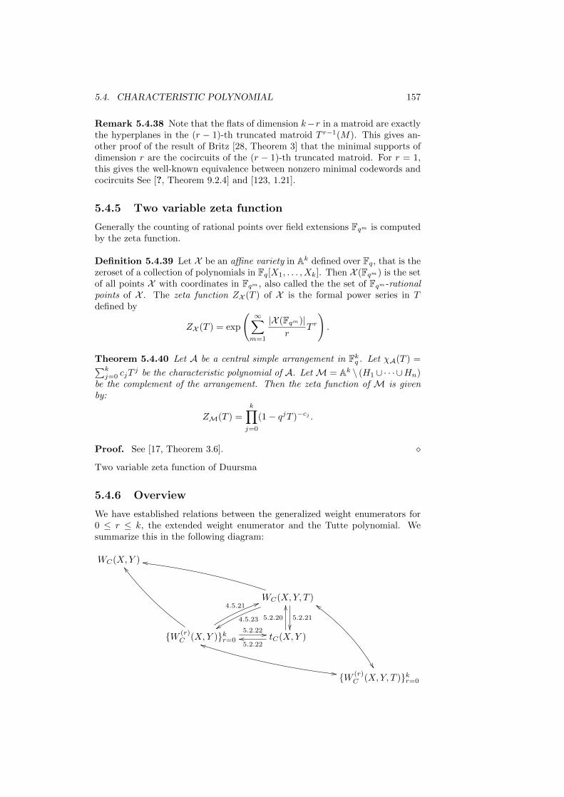
5.4. CHARACTERISTIC POLYNOMIAL 157
Remark 5.4.38 Note that the flats of dimension k−r in a matroid are exactlythe hyperplanes in the (r − 1)-th truncated matroid T r−1(M). This gives an-other proof of the result of Britz [28, Theorem 3] that the minimal supports ofdimension r are the cocircuits of the (r − 1)-th truncated matroid. For r = 1,this gives the well-known equivalence between nonzero minimal codewords andcocircuits See [?, Theorem 9.2.4] and [123, 1.21].
5.4.5 Two variable zeta function
Generally the counting of rational points over field extensions Fqm is computedby the zeta function.
Definition 5.4.39 Let X be an affine variety in Ak defined over Fq, that is thezeroset of a collection of polynomials in Fq[X1, . . . , Xk]. Then X (Fqm) is the setof all points X with coordinates in Fqm , also called the the set of Fqm -rationalpoints of X . The zeta function ZX (T ) of X is the formal power series in Tdefined by
ZX (T ) = exp
( ∞∑m=1
|X (Fqm)|r
T r
).
Theorem 5.4.40 Let A be a central simple arrangement in Fkq . Let χA(T ) =∑kj=0 cjT
j be the characteristic polynomial of A. Let M = Ak \ (H1 ∪ · · · ∪Hn)be the complement of the arrangement. Then the zeta function of M is givenby:
ZM(T ) =
k∏j=0
(1− qjT )−cj .
Proof. See [17, Theorem 3.6].
Two variable zeta function of Duursma
5.4.6 Overview
We have established relations between the generalized weight enumerators for0 ≤ r ≤ k, the extended weight enumerator and the Tutte polynomial. Wesummarize this in the following diagram:
WC(X,Y )
WC(X,Y, T )
4.5.23yy
5.2.21
mm
W (r)C (X,Y )kr=0
4.5.2155
5.2.22 //
[[
tC(X,Y )5.2.22oo
5.2.20
OO
W (r)C (X,Y, T )kr=0
--
jj
cc
158 CHAPTER 5. CODES AND RELATED STRUCTURES
We see that the Tutte polynomial, the extended weight enumerator and thecollection of generalized weight enumerators all contain the same amount of in-formation about a code, because they completely define each other. The originalweight enumerator WC(X,Y ) contains less information and therefore does not
determine WC(X,Y, T ) or W (r)C (X,Y )kr=0. See Simonis [109].
One may wonder if the method of generalizing and extending the weight enu-merator can be continued, creating the generalized extended weight enumerator,in order to get a stronger invariant. The answer is no: the generalized extendedweight enumerator can be defined, but does not contain more information thenthe three underlying polynomials.It was shown by Gray [29] that the matroid of a code is a stronger invariantthan its Tutte polynomial.
5.4.7 Exercises
5.4.1 Give a proof of the formulas in Example 5.4.6.
5.4.2 Give a proof of Remark 5.4.25.
5.4.3 Compute the two variable Mobius and coboundary polynomial of thesimplex code S3(q).
5.5 Combinatorics and codes
***Intro***
5.5.1 Orthogonal arrays and codes
Definition 5.5.1 Let q be a positive integer, not necessarily a power of a prime.A Latin square of order q is a q×q array with entries from a set Q of q elements,such that every column and every row is a permutation of the symbols Q.
Example 5.5.2 An example of a Latin square of order 4 with Q = a, b, c, dis given by
a d c bd a b cc b a db c d a
Remark 5.5.3 An alternative way to represent a Latin square is by a mapL : R × C → Q, where R, C and Q, are the sets of rows, columns and values,respectively, with all three of size q. Then L represents a Latin square if andonly if L(x, j) = k has a unique solution x ∈ R, for all j ∈ C and k ∈ Q, andL(i, y) = k has a unique solution y ∈ C, for all i ∈ R and k ∈ Q.Any permutation of the rows, that is of the set R, gives another Latin square,and similarly permutations of the columns C and the entries Q give again Latinsquares.
Example 5.5.4 Let (G, ·) be a group where · is the multiplication on G. LetR, C and Q all three be equal to G. Let L(x, y) = x · y. Then L defines a Latinsquare of order |G|.
5.5. COMBINATORICS AND CODES 159
Remark 5.5.5 A pair of Greek-Latin squares.Euler’s problem of 36 officers and the non-existence of two mutual orthogonalLatin squares of the order 6.
Definition 5.5.6 Two Latin squares L1 and L2 are called mutually orthogonalifQ2 is equal to the set of all pairs (L1(x, y), L2(x, y)) with x, y ∈ Q. A collectionLi : i ∈ J of Latin squares Li of order q with entries from a set Q, is calleda set of mutually orthogonal Latin squares (MOLS) if Li and Lj are mutualorthogonal for all i, j ∈ J with i 6= j.
Example 5.5.7 Consider Q = Fq where + is the addition. Let La(x, y) =x + ay. Then La defines a Latin square of order q for all a ∈ F∗q . FurthermoreLa : a ∈ F∗q form a collection of q − 1 MOLS of order q.
Example 5.5.8 In GAP one can constructs lists of MOLS. For example forq = 7 we can construct 6 MOLS:> M:=MOLS(7,6);;
> M[1];
[ [ 0, 1, 2, 3, 4, 5, 6 ], [ 1, 2, 3, 4, 5, 6, 0 ], \\
[ 2, 3, 4, 5, 6, 0, 1 ],[ 3, 4, 5, 6, 0, 1, 2 ], \\
[ 4, 5, 6, 0, 1, 2, 3 ], [ 5, 6, 0, 1, 2, 3, 4 ], \\
[ 6, 0, 1, 2, 3, 4, 5 ] ]
Definition 5.5.9 Let n ≥ 2. An orthogonal array OA(q, n) of order q anddepth n is a q2×n array whose entries are from a set Q of q elements, such thatfor every two columns all q2 pairs of symbols from Q appear in exactly one row.
Remark 5.5.10 Let J = 1, 2, . . . , j. Let Li : i ∈ J be a collection of jMOLS of order q. Let n = j + 2. We can construct a q2 × n orthogonal arrayas follows. Identify R and C with Q by means of bijections. So we may assumethat they are equal. In the first two columns all q2 pairs of Q2 are tabulated. If(x, y) is in the row of the first two columns, then Li(x, y) is in the column i+ 2of the same row.Conversely an OA(q, n) gives rise to n − 2 MOLS of order q if n ≥ 3. Inparticular an OA(q, 3) is a Latin square and an OA(q, 4) corresponds to twomutual orthogonal Latin squares.
Example 5.5.11 Let q be a power of a prime. Then a collection of q − 1MOLS of order q is constructed in Example 5.5.7. Therefore there exists anOA(q, q + 1).
Remark 5.5.12 Let Li : i ∈ J be a collection of n − 2 MOLS of order qwith an array A the corresponding OA(q, n). A permutation σ of the rowsR gives a collection L′i : i ∈ J of Latin squares which are again mutuallyorthogonal with a corresponding array A1. Then A1 is obtained from A bypermuting the symbols in the first column under σ and leaving the remainingcolumns unchanged. Similarly, a permutation of the columns C gives an arrayA2 that is obtained from A by permuting the symbols in the second column. Apermutation of the entries from Q of Li gives an array Ai+2 that is obtainedfrom A by permuting the symbols in the (i+ 2)-th column.
160 CHAPTER 5. CODES AND RELATED STRUCTURES
Remark 5.5.13 Let A be an OA(q, n) with entries in Q. Then two rows of Aare distinct and coincide in at most one position. Let C be the subset of Qnconsisting of the rows of A. Then C is a nonlinear code of length n with q2
codewords and minimum distance n − 1. So C attains the Singleton bound ofExercise 3.2.1. Conversely any nonlinear (n, q2, n− 1) code yields an OA(q, n).The following proposition is a generalization of Proposition 4.4.25 in case k = 2,that is n ≤ q + 1 if there exists an [n, 2, n− 1] code over Fq.
Proposition 5.5.14 Suppose there exists an orthogonal array OA(q, n). Thenn ≤ q + 1.
Proof. Let A be the array of an OA(q, n). Choose an element in Q and denoteit by 0. If the symbols in the the i-th column of A are permuted, where theother columns remain unchanged, the new array is again OA(q, n) by Remark5.5.12. Therefore we may assume without loss of generality that the first row ofA consists of zeros. The distance between two rows is at least n− 1 by Remark5.5.13. Hence apart form the first row, no other row contains two zeros. Next,it can be easily observed that each element from Q occurs in every column of Aexactly q times. We leave this as an exercise for the reader.Count the number of rows that contain one zero. This number is n(q − 1).Indeed, zero should appear n times in each column, but zero in the first columnhas already been counted. In addition, since the i-th row with i > 1, cannothave more than one zero, we see that all these zeros lie in different rows. So1 + n(q − 1) is the number of rows that contain a zero, and this is at most q2,the total number of rows. Therefore n ≤ q + 1.
Remark 5.5.15 The bound of Proposition 5.5.14 is tight if q is a power of aprime by Example 5.5.11.
Consider the following generalization of an orthogonal array.
Definition 5.5.16 An orthogonal array OA(q, n, λ) is a λq2 × n array whoseentries are from a set Q of q elements, such that for every two columns any ofq2 pairs of symbols from Q occurs in exactly λ rows. In particular OA(q, n) =OA(q, n, 1).
The next result we present here without a proof. It provides a lower bound onthe value of λ in terms of q and n.
Theorem 5.5.17 If there exists an orthogonal array OA(q, n, λ), then
λ ≥ n(q − 1) + 1
q2.
Proof. Reference: ***...**
Definition 5.5.18 An orthogonal array OAλ(t, n, q) is an M × n array, whereM = λqt, whose entries are from a set Q of q ≥ 2 elements, such that for everyM × t subarray all qt possible t-tuples occur exactly λ times as a row. Theparameters λ, t, n, q and M are called the index, strength, constraints, levelsand size, respectively. The orthogonal array is called linear if Q = Fq and therows of the array form an Fq-linear subspace of Fnq .
5.5. COMBINATORICS AND CODES 161
Remark 5.5.19 An OA(q, n, λ) is an orthogonal array of strength 2, that isOA(q, n, λ) = OAλ(2, n, q). ***Notice that the order of n and q is interchangedaccording to the literature!!! should we adopt this convention too???***
Theorem 5.5.20 The following objects correspond to each other:1) An Fq-linear [n, k, d] code,2) A linear orthogonal array OAqs(d − 1, n, q), where s = n − k + 1 − d is theSingleton defect of C.
Proof. Let C be an Fq-linear [n, k, d] code with Singleton defect s = s(C) =n − k + 1 − d. Consider the qn−k × n matrix A having as rows the codewordsof C⊥. Then A is a linear OAqs(d− 1, n, q). *** ....***
Remark 5.5.21 An OA1(n − k, n, q) is a nonlinear generalization of an Fq-linear MDS code of length n and dimension k.
Consider the following a generalization of Corollary 4.4.27 on MDS codes.
Theorem 5.5.22 (Bush bound) Let A be an OA1(k, n, q). If q ≤ k, thenn ≤ k + 1.
Proof. ***... ***
5.5.2 Designs and codes
5.5.3 Exercises
5.5.1 Proof that Example 5.5.7 gives a set of q− 1 mutually orthogonal Latinsquares of order q.
5.5.2 Let q be positive integer. Show that q − 1 is the maximal number ofMOLS of order q.
5.5.3 Show that there exist t MOLS of order qr if there exist t MOLS of ordersq and r, respectively.
5.5.4 Let n ≥ 3. Give a proof of the correspondence between an OA(q, n) andn− 2 MOLS of order q of Remark 5.5.10.
5.5.5 Let A be the array of an OA(q, n, λ) with entries from Q. Show thatevery symbol of Q occurs in every column of A exactly λq times.
5.5.6 Let A be the array of an OAλ(t, q, n) with entries from Q. Let A′ beobtained from A by permuting the symbols in a given column and leaving theremaining columns unchanged. Show that A′ is the array of an OAλ(t, q, n).
5.5.7 [CAS] Write two procedures:
• first takes as an input a q x q table and checks if the table is a Latinsquare. Check your procedure with IsLatinSquare in GAP;
• second given a list of q x q tables checks if they are MOLS. Use AreMOLS
from GAP to test your procedure.
162 CHAPTER 5. CODES AND RELATED STRUCTURES
5.6 Notes
Section 4.1.6: MDS Conjecture is confirmed for all q such that 2 ≤ q ≤ 11,Blokhuis-Bruen-Thas, Hirschfeld-Storme.
Section 4.2:
Theory of arrangements of hyperplanes [92].
The use of the isomorphism in Proposition 4.5.18 for the proof of Theorem4.5.21 was suggested in [109] by Simonis.
Proposition 4.5.20 first appears in [63, Theorem 3.2], although the term “gen-eralized weight enumerator” was yet to be invented.
The identity of Lemma 4.5.22 one can find in [5, 27, 71, 128, 113].
Section 4.3:
Applications of GHW’s***dimension/length profile, Forney******Wire-tap channel of type II******trellis complexity***
***r-th rank MDS, Kloeve,Simonis,Wei******Question: two var. wt enumerator determines the generalized wit enumera-tor?******C AMDS C⊥ AMDS iff d2 = d1 + 2.******If d > qs(C), then ...****** wt enumerator of AMDS code***
Section: 4.4:
Theory of lattices [38, ?].
The polynomial µL(S, T ) is defined by Zaslavsky in [139, Section 1]. In [140,Section 2]. and [?, Section 6] it is called the Whitney polynomial. The polyno-mial χL(S, T ) is called the coboundary polynomial by Crapo in [42, p. 605] and[43]. See also [30, 32].
Blocking sets and codes meeting the Griesmer bound
minihypers, blocking sets and codes meeting the Griesmer bound
Belov, Hamada-Helleseth, Storme
Section 4.4.2: Corollary 4.3.25 was proved first Oberst and Dur [?], with theweaker assumption qm >
(n−1d−1
)−(n−k−1d−1
), where C is an [n, k, d] code. Propo-
sition 4.3.24 was shown by Pellikaan [?] with a stronger conclusion.
5.6. NOTES 163
(Complete) n-arcs, ovals, Segre: an oval is (q + 1)-arc if q is odd, ***B. Segre,conic, odd curve in char 2, nucleus***Conjectures of Segre, Hirschfeld-Thas, Hirschfeld-Kochmaros-Torres pp. 599.
Section: 4.5:
Section 4.6:
Literature on (mutual orthogonal) Latin squares, orthogonal arrays, codes anddesigns:
J.H. van Lint and R.M. Wilson: A course in combinatorics Pages: 158, 250,261, 382 and 495.
P. Cameron and J.H. van Lint Designs, graphs, codes and their links. Pages:14, 93, 170, 209.
Links between coding theory and statistical objects:
R.C. Bose, “On some connections between the design of experiments and infor-mation theory,” Bull. Inst. Internat. Statist., vol. 38, pp. 257–271, 1961.
Connection between OA and Error-correcting codes with a given defect: R.C.Bose and K.A. Bush, “Orthogonal arrays of strength two and three,” Ann.Math. Stat., vol 23, pp. 508–524, 1952.
The construction of OA of max length and the Bush bound.K.A. Bush, “Orthogonal arrays of index unity,” Ann. Math. Stat., vol 23, pp.426–434, 1952.
J.W.P. Hirschfeld and L. Storme, “The packing problem in statistics, codingtheory and finite projective spaces,” Journ. Stat. Planning and Inference, vol.72, pp. 355–380, 1998.
The notion of a OAλ(t, q, n) as a generalization of MOLS is from:C.R. Rao, “Factorial experiments derivable from combinatorial arrangements ofarrays,” Journ. Royal Stat. Soc. Suppl. vol. 9, pp. 128–139, 1947.
***Bose-Bush,Bierbrauer, Stinson******t-resilient functions,
***The design of statistical experiments.
***Lattices and codes.

164 CHAPTER 5. CODES AND RELATED STRUCTURES
Chapter 6
Complexity and decoding
Stanislav Bulygin, Ruud Pellikaan and Xin-Wen Wu
6.1 Complexity
In this section we briefly explain the theory of complexity and introduce somehard problems which are related to the theme of this book and will be useful inthe following chapters.
6.1.1 Big-Oh notation
The following definitions and notations are essential in the evaluation of thecomplexity of an algorithm.
Definition 6.1.1 Let f(n) and g(n) be functions mapping non-negative inte-gers to real numbers. We define
(1) f(n) = O(g(n)) for n → ∞, if there exists a real constant c > 0 and aninteger constant n0 > 0 such that 0 ≤ f(n) ≤ cg(n) for all n ≥ n0.
(2) f(n) = Ω(g(n)) for n → ∞, if there exists a real constant c > 0 and aninteger constant n0 > 0 such that 0 ≤ cg(n) ≤ f(n) for all n ≥ n0.
(3) f(n) = Θ(g(n)) for n→∞, if there exist real constants c1 > 0 and c2 > 0,and an integer constant n0 > 0 such that c1g(n) ≤ f(n) ≤ c2g(n) for alln ≥ n0.
(4) f(n) ≈ g(n) for n→∞, if limn→∞ f(n)/g(n) = 1.
(5) f(n) = o(g(n)) for n→∞, if for every real constant ε > 0 there exists aninteger constant n0 > 0 such that 0 ≤ f(n) < εg(n) for all n ≥ n0.
Remark 6.1.2 The notations f(n) = O(g(n)) and f(n) = o(g(n)) of Landauare often referred to as the “big-Oh” and “little-oh” notations. Furthermoref(n) = O(g(n)) is expressed as “f(n) is of the order g(n)”. Intuitively, thismeans that f(n) grows no faster asymptotically than g(n) up to a constant. And
165
166 CHAPTER 6. COMPLEXITY AND DECODING
f(n) ≈ g(n) is expressed as “f(n) is approximately equal to g(n)”. Similarly,in the literature f(n) = Ω(g(n)) and f(n) = Θ(g(n)), are referred to as the“big-Omega”, “big-Theta”, notations, respectively.
Example 6.1.3 It is easy to see that for every positive constant a, we havea = O(1) and a/n = O(1/n). Let f(n) = akn
k + ak−1nk−1 + · · ·+ a0, where k
is an integer constant and ak, ak−1, . . . , a0 are real constants with ak > 0. Forthis polynomial in n, we have f(n) = O(nk), f(n) = Θ(nk), f(n) ≈ akn
k andf(n) = o(nk+1) for n→∞.
We have 2 log n + 3 log logn = O(log n), 2 log n + 3 log log n = Θ(log n) and2 log n + 3 log log n ≈ 2 log n for n → ∞, since 2 log n ≤ 2 log n + 3 log log n ≤5 log n when n ≥ 2 and limn→∞ log log n/ log n = 0.
6.1.2 Boolean functions
An algorithm is a well-defined computational procedure such that every execu-tion takes a variable input and halts with an output.
The complexity of an algorithm or a computational problem includes time com-plexity and storage space complexity.
Definition 6.1.4 A (binary) elementary (arithmetic) operation is an addition,a comparison or a multiplication of two elements x, y ∈ 0, 1 = F2. Let A bean algorithm that has as input a binary word. Then the time or work complexityCT (A, n) is the number of elementary operations in the algorithm A to get theoutput as a function of the length n of the input, that is the number of bits ofthe input. The space or memory complexity CT (A, n) is the maximum numberof bits needed for memory during the execution of the algorithm with an inputof n bits. The complexity C(A, n) is the maximum of CT (A, n) and CS(A, n).
Example 6.1.5 Let C be a binary [n, k] code given the generator matrix G.Then the encoding procedure
(a1, . . . , ak) 7→ (a1, . . . , ak)G
is an algorithm. For every execution of the encoding algorithm, the input is avector of length k which represents a message block; the output is a codewordof length n. To compute one entry of a codeword one has to perform k multipli-cations and k − 1 additions. The work complexity of this encoding is thereforen(2k − 1). The memory complexity is nk + k + n: the number of bits neededto store the input vector, the matrix G and the output codeword. Thus thecomplexity is dominated by work complexity and thus is n(2k − 1).
Example 6.1.6 In coding theory the code length is usually taken as a measureof an input size. In case of binary codes this coincides with the above complexitymeasures. For q-ary codes an element of Fq has a minimal binary representationby dlog(q)e bits. A decoding algorithm with a received word of length n as inputcan be represented by a binary word of length N = ndlog(q)e. In case the finitefield is fixed there is no danger of confusion, but in case the efficiency of algo-rithms for distinct finite fields are compared, everything should be expressed in
6.1. COMPLEXITY 167
terms of the number of binary elementary operations as a function of the lengthof the input as a binary string.
Let us see how this works out for solving a system of linear equations over afinite field. Whereas the addition and multiplication is counted for 1 unit inthe binary case, this is no longer the case in the q-ary case. An addition inFq is equal to dlog(q)e binary elementary operations and multiplication needsO(m2 log2(p) + m log3(p)) = O(log3(q)) elementary operations, where q = pm
and p is the characteristic of the finite field, see ??. The Gauss-Jordan algorithmto solve a system of n linear equations in n unknowns over a finite field Fq needsO(n3) additions and multiplications in Fq. That means the binary complexity isO(n3 log3(q)) = O(N3), where N = ndlog(q)e is the length of the binary input.The known decoding algorithms that have polynomial complexity and that willbe treated in the sequel reduce all to linear algebra computations, so they havecomplexity O(n3) elementary operations in Fq or O(N3) bit operations. Sowe will take the code length n as a measure of the input size, and state thecomplexity as a function of n. These polynomial decoding algorithms apply torestricted classes of linear codes.
To study the theory of complexity, two different computational models whichboth are widely used in the literature are the Turing machine (TM) model andBoolean circuit model. Between these two models the Boolean circuit model hasan especially simple definition and is viewed more amenable to combinatorialanalysis. A Boolean circuit represents a Boolean function in a natural way.And Boolean functions have a lot of applications in the theory of coding. Inthis book we choose Boolean circuits as the computational model.
*** One of two paragraphs on Boolean Circuits vs. Turing Machines (c.f. R.B.Boppana & M. Sipser, ”The Complexity of Finite Function”) ***
The basic elements of a Boolean circuit are Boolean gates, namely, AND, OR,NOT, and XOR, which are defined by the following truth tables.
The truth table of AND (denoted by ∧):
∧ F TF F FT F T
The truth of OR (denoted by ∨):
∨ F TF F TT T T
The truth table of NOT (denoted by ¬):
¬ F TT F
The truth table of XOR:
168 CHAPTER 6. COMPLEXITY AND DECODING
XOR F TF F TT T F
It is easy to check that XOR gate can be represented by AND, OR and NOTas the following
x XOR y = (x ∧ (¬y)) ∨ ((¬x) ∧ y).
The NAND operation is an AND operation followed by a NOT operation. TheNOR operation is an OR operation followed by a NOT operation. In the fol-lowing definition of Boolean circuits, we restrict to operations AND, OR andNOT.
Substituting F = 0 and T = 1, the Boolean gates above are actually operationson bits (called logical operations on bits). We have
∧ operation:
0 ∧ 0 = 00 ∧ 1 = 01 ∧ 0 = 01 ∧ 1 = 1
∨ operation:
0 ∨ 0 = 00 ∨ 1 = 11 ∨ 0 = 11 ∨ 1 = 1
NOT operation:
¬ 0 = 1¬ 1 = 0
Consider the binary elementary arithmetic operations + and ·. It is easy toverify that
x · y = x ∧ y, and x+ y = x XOR y = (x ∧ (¬y)) ∨ ((¬x) ∧ y).
Definition 6.1.7 Given positive integers n and m, a Boolean function is afunction b : 0, 1n → 0, 1m. It is also called an n-input, m-output Booleanfunction and the set of all such functions is denoted by B(n,m). Denote B(n, 1)by B(n).
Remark 6.1.8 The number of elements of B(n,m) is (2n)2m
= 2n2m
. Identify0, 1 with the binary field F2. Let b1 and b2 be elements of B(n,m). Thenthe sum b1 + b2 is defined by (b1 + b2)(x) = b1(x) + b2(x) for x ∈ Fn2 . In thisway the set of Boolean functions B(n,m) is a vector space over F2 of dimensionn2m. Let b1 and b2 be elements of B(n). Then the product b1b2 is defined by(b1b2)(x) = b1(x)b2(x) for x ∈ Fn2 . In this way B(n) is an F2-algebra with theproperty b2 = b for all b in B(n).
6.1. COMPLEXITY 169
Every polynomial f(X) in F2[X1, . . . , Xn] yields a Boolean function f : Fn2 → F2
by evaluation: f(x) = f(x) for x ∈ Fn2 . Consider the map
ev : F2[X1, . . . , Xn] −→ B(n),
defined by ev(f) = f . Then ev is an algebra homomorphism. Now X2i = Xi
for all i. Hence the ideal 〈X21 +X1, . . . , X
2n +Xn〉 is contained in the kernel of
ev. The factor ring and F2[X1, . . . , Xn]/〈X21 +X1, . . . , X
2n +Xn〉 and B(n) are
both F2-algebras of the same dimension n. Hence ev induces an isomorphism
ev : F2[X1, . . . , Xn]/〈X21 +X1, . . . , X
2n +Xn〉 −→ B(n).
Example 6.1.9 Let symk(x) be the Boolean function defined by the followingpolynomial in k2 variables xij , 1 ≤ i, j ≤ k,
symk(x) =
k∏i=1
k∑j=1
xij .
Hence this description needs k(k−1) additions and k−1 multiplications. There-fore k2− 1 elementary operations are needed in total. If we would have writtensymk in normal form by expanding the products, the description is of the form
symk(x) =∑σ∈KK
k∏i=1
xiσ(i),
where KK is the set of all functions σ : 1, . . . , k → 1, . . . , k . This expressionhas kk terms of products of k factors. So this needs (k − 1)kk multiplicationsand kk − 1 additions. Therefore kk+1 − 1 elementary operations are needed intotal. Hence this last description has exponential complexity.
Example 6.1.10 Computing the binary determinant. Let detk(x) be the Booleanfunction of k2 variables xij , 1 ≤ i, j ≤ k, that computes the determinant overF2 of the k × k matrix x = (xij). Hence
detk(x) =∑σ∈Sk
k∏i=1
xiσ(i),
where Sk is the symmetric group of k elements. This expression has k! terms ofproducts of k factors. Therefore k(k!)− 1 elementary operations are needed intotal.Let xij be the the square matrix of size k− 1 obtained by deleting the i-th rowand the j-th column from x. Using the cofactor expansion
detk(x) =
k∑j=1
xijdetk(xij),
we see that the complexity of this computation is of the order O(k!). Thiscomplexity is still exponential. But detk has complexity O(k3) by Gaussianelimination. This translates in a description of detk as a Boolean function withO(k3) elementary operations.***explicit description and worked out in and example in det3.***
170 CHAPTER 6. COMPLEXITY AND DECODING
Example 6.1.11 A Boolean function computing whether an integer is primeor not. Let primem(x) be the Boolean function that is defined by
primem(x1, . . . , xm) =
1 if x1 + x22 + · · ·+ xm2m−1 is a prime,0 otherwise.
So prime2(x1, x2) = x2 and prime3(x1, x2, x3) = x2 + x1x3 + x2x3.Only very recently it was proved that the decision problem whether an integeris prime or not, has polynomial complexity, see ??.
Example 6.1.12 ***A Boolean function computing exponentiation expa byCoppersmith and Shparlinski, “A polynomial approximation of DL and DHmapping,” Journ. Crypt. vol. 13, pp. 339–360, 2000. ***
Remark 6.1.13 From these examples we see that the complexity of a Booleanfunction depends on the way we write it as a combination of elementary opera-tions.
We can formally define the complexity of a Boolean function f in terms of thesize of a circuit that represents the Boolean function.
Definition 6.1.14 A Boolean circuit is a directed graph containing no cycles(that is, if there is a route from any node to another node then there is no wayback), which has the following structure:
(i) Any node (also called vertex ) v has in-degree (that is, the number of edgesentering v) equal to 0, 1 or 2, and the out-degree (that is, the number ofedges leaving v) equal to 0 or 1.
(ii) Each node is labeled by one of AND, OR, NOT, 0, 1, or a variable xi.
(iii) If a node has in-degree 0, then it is called an input and is labeled by 0, 1,or a variable xi.
(iv) If a node has in-degree 1 and out-degree 1, then it is labeled by NOT.
(v) If a node has in-degree 2 and out-degree 1, then it is labeled by AND orOR.
In a Boolean circuit, any node with in-degree greater than 0 is called a gate.Any node with out-degree 0 is called an output.
Remark 6.1.15 By the definition, we observe that:
(1) A Boolean circuit can have more than one input and more than one output.
(2) Suppose a Boolean circuit has n variables x1, x2, . . . , xn, and has m out-puts, then it represents a Boolean function f : 0, 1n → 0, 1m in anatural way.
(3) Any Boolean function f : 0, 1n → 0, 1m can be represented by aBoolean circuit.
6.1. COMPLEXITY 171
Definition 6.1.16 The size of a Boolean circuit is the number of gates thatit contains. The depth of a Boolean circuit is the length of the longest pathfrom an input to an output. For a Boolean function f , the time complexity off , denoted by CT (f), is the smallest value of the sizes of the Boolean circuitsrepresenting f . The space complexity (also called depth complexity), denoted byCS(f) is the smallest value of the depths of the Boolean circuits representing f .
Theorem 6.1.17 (Shannon) Existence of a family of Boolean function of ex-ponential complexity.
Proof. Let us first give a upper bound on the number of circuits with nvariables and size s; and then compare it with the number of Boolean functionsof n variables.
In a circuit of size s, each gate is assigned an AND or OR operator that on twoprevious nodes *** this phrase is strangely stated. ***. Each previous node caneither be a previous gate with at most s choices, a literal (that is, a variable orits negation) with 2n choices, or a constant with 2 choices. Therefore, each gatehas at most 2(s+2n+2)2 choices, which implies that the number of circuits withn variables and size s is at most 2s(s + 2n + 2)2s. Now, setting s = 2n/(10n),the upper bound 2s(s+ 2n+ 2)2s is approximately 22n/5 22n
. On the otherhand, the number of Boolean functions of n variables and one output is 22n
.This implies that almost every Boolean function requires circuits of size largerthan 2n/(10n).
6.1.3 Hard problems
We now look at the classification of algorithms through the complexity.
Definition 6.1.18 Let
Ln(α, a) = O(exp(anα(lnn)1−α)),
where a and α are constants with 0 ≤ a and 0 ≤ α ≤ 1. In particularLn(1, a) = O(exp(an)), and Ln(0, a) = O(exp(a lnn)) = O(na). Let A denotean algorithm with input size n. Then A is an L(α)-algorithm if the complexityof this algorithm has an estimate of the form Ln(α, a) for some a. An L(0)-algorithm is called a polynomial algorithm and an L(1)-algorithm is called anexponential algorithm. An L(α)-algorithm is called an subexponential algorithmif α < 1.
A problem that has either YES or NO as an answer is called a decision problem.All the computational problems that will be encountered here can be phrasedas decision problems in such a way that an efficient algorithm for the decisionproblem yields an efficient algorithm for the computational problem, and viceversa. In the following complexity classes, we restrict our attention to decisionproblems.
Definition 6.1.19 The complexity class P is the set of all decision problemsthat are solvable in polynomial complexity.
172 CHAPTER 6. COMPLEXITY AND DECODING
Definition 6.1.20 The complexity class NP is the set of all decision problemsfor which a YES answer can be verified in polynomial time given some extrainformation, called a certificate. The complexity class co-NP is the set of alldecision problems for which a NO answer can be verified in polynomial timegiven an appropriate certificate.
Example 6.1.21 Consider the decision problem that has as input a generatormatrix of a code C and a positive integer w, with question “d(C) ≤ w?” In casethe answer is yes, there exists a codeword c of minimum weight d(C). Then cis a certificate and the verification wt(c) ≤ w has complexity n.
Definition 6.1.22 Let D1 and D2 be two computational problems. Then D1
is said to polytime reducible to D2, denoted as D1 ≤P D2, provided that thereexists an algorithm A1 that solves D1 which uses an algorithm A2 that solvesD2, and A1 runs in polynomial time if A2 does. Informally, if D1 ≤P D2, wesay D1 is no harder than D2. If D1 ≤P D2 and D2 ≤P D1, then D1 and D2 aresaid to be computationally equivalent.
Definition 6.1.23 A decision problem D is said to be NP-complete if
• D ∈ NP, and
• E ≤P D for every E ∈ NP.
The class of all NP-complete problems is denoted by NPC.
Definition 6.1.24 A computational problem (not necessarily a decision prob-lem) is NP-hard if there exists some NP-complete problem that polytime re-duces to it.
Observe that every NP-complete problem is NP-hard. So the set of all NP-hard problems contains NPC as a subset. Some other relationships among thecomplexity classes above are illustrated as follows.
******A Figure******
It is natural to ask the following questions
(1) Is P = NP ?
(2) Is NP = co-NP ?
(3) Is P = NP ∩ co-NP ?
Most experts are of the opinion that the answer to each of these questions is NO.However no mathematical proofs are available, and to answer these questions isan interesting and hard problem in theoretical computer science.
6.1.4 Exercises
6.1.1 Give an explicit expression of det3(x) as a Boolean function.
6.1.2 Give an explicit expression of prime4(x) as a Boolean function.
6.1.3 Give an explicit expression of expa(x) as a Boolean function, where ....
6.2. DECODING 173
6.2 Decoding
*** intro***
6.2.1 Decoding complexity
The known decoding algorithms that work for all linear codes have exponentialcomplexity. Now we consider some of them.
Remark 6.2.1 The brute force method compares the distance of a receivedword with all possible codewords, and chooses a codeword of minimum distance.The time complexity of the brute force method is at most nqk.
Definition 6.2.2 Let r be a received word with respect to a code C of dimen-sion k. Choose an (n − k) × n parity check matrix H of the code C. Thens = rHT ∈ Fn−kq is called the syndrome of r.
Remark 6.2.3 Let C be a code of dimension k. Let r be a received word.Then r + C is called the coset of r. Now the cosets of the received words r1
and r2 are the same if and only if r1HT = r2H
T . Therefore there is a one toone correspondence between cosets of C and values of syndromes. Furthermoreevery element of Fn−kq is the syndrome of some received word r, since H has
rank n− k. Hence the number of cosets is qn−k.
Remark 6.2.4 In Definition 2.4.10 of coset leader decoding no mention is givenof how this method is implemented. Cosetleader decoding can be done in twoways. Let H be a parity check matrix and G a generator matrix of C.1) Preprocess a look-up table and store it in memory with a list of pairs (s, e),where e is a coset leader of the coset with syndrome s ∈ Fn−kq .
Suppose a received word r is the input, compute s = rHT ; look at the uniquepair (s, e) in the table with s as its first entry; give r− e as output.2) For a received word r, compute s = rHT ; compute a solution e of minimalweight of the equation eHT = s; give r− e as output.
Now consider the complexity of the two methods for coset leader decoding:1) The space complexity is clearly qn−k the number of elements in the table. Thetime complexity is O(k2(n−k)) for finding the solution c. The preprocessing ofthe table has time complexity qn−k by going through all possible error patternse of non-decreasing weight and compute s = eHT . Put (s, e) in the list if s isnot already a first entry of a pair in the list.2) Go through all possible error patterns e of non-decreasing weight and computes = eHT and compare it with rHT , where r is the received word. The firstinstance where eHT = rHT gives a closest codeword c = r−e. The complexityis at most |Bρ|n2 for finding a coset leader, where ρ is the covering radius, byRemark 2.4.9.***Now |Bρ| ≈ ... ***
Example 6.2.5 ***[7,4,3] Hamming codes and other perfect codes, some smallnon perfect codes.***
In order to compare their complexities we introduce the following definitions.***work factor, memory factor***
174 CHAPTER 6. COMPLEXITY AND DECODING
Definition 6.2.6 Let the complexity of an algorithm be exponential O(qen)for n→∞. Then e is called the complexity exponent of the algorithm.
Example 6.2.7 The complexity exponent of the brute force method is R andof coset leader decoding is 1−R, where R is the information rate.
***Barg, van Tilburg. picture***
6.2.2 Decoding erasures
***hard/soft decision decoding, (de)modulation, signalling***
After receiving a word there is a stage at the beginning of the decoding processwhere a decision has to be made about which symbol has been received. Insome applications it is desirable to postpone a decision and to put a questionmark ”?” as a new symbol at that position, as if the symbol was erased. This iscalled an erasure. So a word over the alphabet Fq with erasures can be viewedas a word in the alphabet Fq ∪ ?, that is an element of (Fq ∪ ?)n. If onlyerasures occur and the number of erasures is at most d−1, then we are sure thatthere is a unique codeword that agrees with the received word at all positionsthat are not an erasure.
Proposition 6.2.8 Let d be the minimum distance of a code. Then for everyreceived word with t errors and s erasures such that 2t+ s < d there is a uniquenearest codeword. Conversely, if d ≤ 2t + s then there is a received word withat most t errors and s erasures with respect to more than one codeword.
Proof. This is left as an exercise to the reader.
Suppose that we have received a word with s erasures and no errors. Thenthe brute force method would fill in all the possible qs words at the erasurepositions and check whether the obtained word is a codeword. This method hascomplexity O(n2qs), which is exponential in the number of erasures. In thissection it is shown that correcting erasures only by solving a system of linearequations. This can be achieved by using the generator matrix or the paritycheck matrix. The most efficient choice depends on the rate and the minimumdistance of the code.
Proposition 6.2.9 Let C be a code in Fnq with parity check matrix H andminimum distance d. Suppose that the codeword c is transmitted and the word ris received with no errors and at most d−1 erasures. Let J be the set of erasurepositions of r. Let y ∈ Fnq be defined by yj = rj if j 6∈ J and yj = 0 otherwise.
Let s = yHT be the syndrome of y. Let e = y− c. Then wt(e) < d and e is theunique solution of the following system of linear equations in x:
xHT = s and xj = 0 for all j 6∈ J.
Proof. By the definitions we have that
s = yHT = cHT + eHT = 0 + eHT = eHT .
6.2. DECODING 175
The support of e is contained in J . Hence ej = 0 for all j 6∈ J . Therefore e is asolution of the system of linear equations.If x is another solution, then (x− e)HT = 0. Therefore x− e is an element ofC, and moreover it is supported at J . So its weight is at most d(C)− 1. Henceit must be zero. Therefore x = e.
The above method of correcting the erasures only by means of a parity checkmatrix is called syndrome decoding up to the minimum distance.
Definition 6.2.10 Let the complexity of an algorithm be f(n) with f(n) ≈ cnefor n→∞. Then the algorithm is called polynomial of degree e with complexitycoefficient c.
Corollary 6.2.11 The complexity of correcting erasure only by means of syn-drome decoding up to the minimum distance is polynomial of degree 3 and com-plexity coefficient 1
3 (1 − R)2δ for a code of length n → ∞, where R is theinformation rate and δ the relative minimum distance.
Proof. This is consequence of Proposition 6.2.9 which amounts to solving asystem of n− k linear equations in at most d− 1 unknowns, in order to get theerror vector e. Then c = y − e is the codeword sent. We may assume that theencoding is done systematically at k positions, so the message m is immediatelyread off from these k positions. The complexity is asymptotically of the order:13 (n− k)2d = 1
3 (1−R)2δn3 for n→∞. See Appendix ??.
Example 6.2.12 Let C be the binary [7, 4, 3] Hamming code with parity checkmatrix given in Example 2.2.9. Suppose that r = (1, 0, ?, ?, 0, 1, 0) is a receivedword with two erasures. Replace the erasures by zeros by y = (1, 0, 0, 0, 0, 1, 0).The syndrome of y is equal to yHT = (0, 0, 1). Now we want to solve the systemof linear equations xHT = (1, 1, 0) and xi = 0 for all i 6= 3, 4. Hence x3 = 1 andx4 = 1 and c = (1, 0, 1, 1, 0, 1, 0) is the transmitted codeword.
Example 6.2.13 Consider the MDS code C1 over F11 of length 11 and dimen-sion 4 with generator matrix G1 as given in Proposition 3.2.10 with xi = i ∈ F11
for i = 1, . . . , 11. Let C be the dual code of C1. Then C is a [11, 7, 5] code byCorollary 3.2.7, and H = G1 is a parity check matrix for C by Proposition2.3.19. Suppose that we receive the following word with 4 erasures and noerrors.
r = (1, 0, ?, 2, ?, 0, 0, 3, ?, ?, 0).
What is the sent codeword ? Replacing the erasures by 0 gives the word
y = (1, 0, 0, 2, 0, 0, 0, 3, 0, 0, 0).
So yHT = (6, 0, 5, 4). Consider the linear system of equations given by the 4×4submatrix of H consisting of the columns corresponding to the erasure positions3, 5, 9 and 10 together with the column HyT .
1 1 1 1 63 5 9 10 09 3 4 1 55 4 3 10 4
.
176 CHAPTER 6. COMPLEXITY AND DECODING
After Gaussian elimination we see that (0, 8, 9, 0)T is the unique solution of thissystem of linear equations. Hence
c = (1, 0, 0, 2, 3, 0, 0, 3, 2, 0, 0)
is the codeword sent.
Remark 6.2.14 Erasures only correction by means of syndrome decoding isefficient in case the information rate R is close to 1 and the relative minimumdistance δ is small, but cumbersome if R is small and δ is close to 1. Takefor instance the [n, 1, n] binary repetition code. Any received word with n − 1erasures is readily corrected by looking at the remaining unerased position, ifit is 0, then the all zero word was sent, and if it is 1, then the all one wordwas sent. With syndrome decoding one should solve a system of n − 1 linearequations in n− 1 unknowns.
The following method to correct erasures only uses a generator matrix of a code.
Proposition 6.2.15 Let G be a generator matrix of an [n, k, d] code C overFq. Let m ∈ Fkq be the transmitted message. Let s be an integer such thats < d. Let r be the received word with no errors and at most s erasures. LetI = j1, . . . , jn−s be the subset of size n − s that is in the complement of theerasure positions. Let y ∈ Fn−sq be defined by yi = rji for i = 1, . . . , n − s.Let G′ be the k × (n − s) submatrix of G consisting of the n − s columns of Gcorresponding to the set I. Then xG′ = y has a unique solution m, and mG isthe codeword sent.
Proof. The Singleton bound 3.2.1 states that k ≤ n − d + 1. So k ≤ n − s.Now mG = c is the codeword sent and yi = rji = cji for i = 1, . . . , n−s. HencemG′ = y and m is a solution. Now suppose that x ∈ Fkq satisfies xG′ = y,then (m − x)G is a codeword that has a zero at n − s positions, so its weightis at most s < d. So (m − x)G is the zero codeword and xG′ = mG′. Hencem− x = 0, since G has rank k.
The above method is called correcting erasures only up to the minimum distanceby means of the generator matrix.
Corollary 6.2.16 The complexity of correcting erasures only up to the mini-mum distance by means of the generator matrix is polynomial of degree 3 andcomplexity coefficient R2(1 − δ − 2
3R) for a code of length n → ∞, where R isthe information rate and δ the relative minimum distance.
Proof. This is consequence of Proposition 6.2.15. The complexity is that ofsolving a system of k linear equations in at most n− d+ 1 unknowns, which isasymptotically of the order: (n − d − 2
3k)k2 = R2(1 − δ − 23R)n3 for n → ∞.
See Appendix ??.
***picture, comparison of G and H method**
Example 6.2.17 Let C be the [7, 2, 6] extended Reed-Solomon code over F7
with generator matrix
G =
(1 1 1 1 1 1 10 1 2 3 4 5 6
)
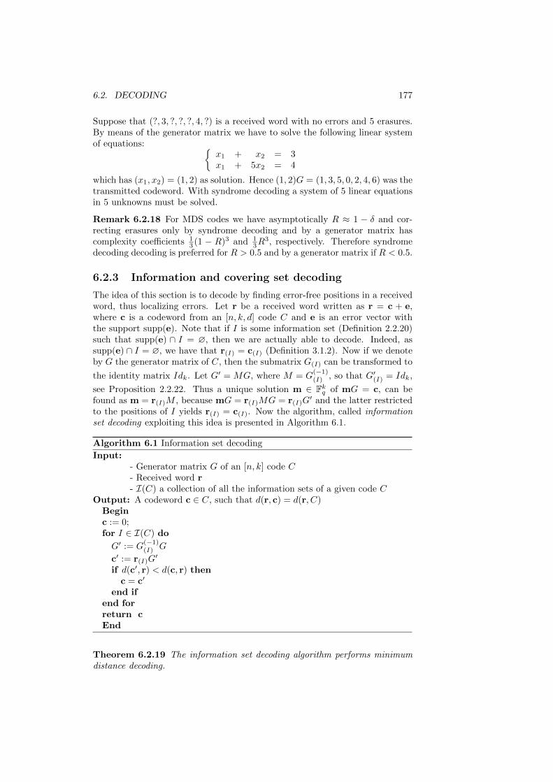
6.2. DECODING 177
Suppose that (?, 3, ?, ?, ?, 4, ?) is a received word with no errors and 5 erasures.By means of the generator matrix we have to solve the following linear systemof equations:
x1 + x2 = 3x1 + 5x2 = 4
which has (x1, x2) = (1, 2) as solution. Hence (1, 2)G = (1, 3, 5, 0, 2, 4, 6) was thetransmitted codeword. With syndrome decoding a system of 5 linear equationsin 5 unknowns must be solved.
Remark 6.2.18 For MDS codes we have asymptotically R ≈ 1 − δ and cor-recting erasures only by syndrome decoding and by a generator matrix hascomplexity coefficients 1
3 (1 − R)3 and 13R
3, respectively. Therefore syndromedecoding decoding is preferred for R > 0.5 and by a generator matrix if R < 0.5.
6.2.3 Information and covering set decoding
The idea of this section is to decode by finding error-free positions in a receivedword, thus localizing errors. Let r be a received word written as r = c + e,where c is a codeword from an [n, k, d] code C and e is an error vector withthe support supp(e). Note that if I is some information set (Definition 2.2.20)such that supp(e) ∩ I = ∅, then we are actually able to decode. Indeed, assupp(e) ∩ I = ∅, we have that r(I) = c(I) (Definition 3.1.2). Now if we denoteby G the generator matrix of C, then the submatrix G(I) can be transformed to
the identity matrix Idk. Let G′ = MG, where M = G(−1)(I) , so that G′(I) = Idk,
see Proposition 2.2.22. Thus a unique solution m ∈ Fkq of mG = c, can befound as m = r(I)M , because mG = r(I)MG = r(I)G
′ and the latter restrictedto the positions of I yields r(I) = c(I). Now the algorithm, called informationset decoding exploiting this idea is presented in Algorithm 6.1.
Algorithm 6.1 Information set decoding
Input:- Generator matrix G of an [n, k] code C- Received word r- I(C) a collection of all the information sets of a given code C
Output: A codeword c ∈ C, such that d(r, c) = d(r, C)Beginc := 0;for I ∈ I(C) do
G′ := G(−1)(I) G
c′ := r(I)G′
if d(c′, r) < d(c, r) thenc = c′
end ifend forreturn cEnd
Theorem 6.2.19 The information set decoding algorithm performs minimumdistance decoding.
178 CHAPTER 6. COMPLEXITY AND DECODING
Proof. Let r = c + e, where wt(e) = d(r, C). Let rH = eH = s. Then eis a coset leader with the support E = supp(e) in the coset with the syndromes. It is enough to prove that there exists some information set disjoint with E,or, equivalently, some check set (Definition 2.3.9) that contains E. Consider an(n − k) × |E| submatrix H(E) of the parity check matrix H. As e is a cosetleader, we have that for no other vector v in the same coset is supp(v) ( E.Thus the subsystem of the parity check system defined by positions from E hasa unique solution e(E). Otherwise it would be possible to find a solution withsupport a proper subset of E. The above implies that rank(H(E)) = |E| ≤ n−k.Thus E can be expanded to a check set.
For a practical application it is convenient to choose the sets I randomly.Namely, we choose some k-subsets randomly in hope that after some reasonableamount of trials we encounter the one that is an information set and error-free.
Algorithm 6.2 Probabilistic information set decoding
Input:- Generator matrix G of an [n, k] code C- Received word r- Number of trials Ntrials(n, k)
Output: A codeword c ∈ CBeginc := 0;Ntr := 0;repeatNtr := Ntr + 1;Choose uniformly at random a subset I of 1, . . . , n of cardinality k.if G(I) is invertible then
G′ := G(−1)(I) G
c′ = r(I)G′
if d(c′, r) < d(c, r) thenc := c′
end ifend if
until Ntr < Ntrials(n, k)
return cEnd
We would like to estimate the complexity of the probabilistic information setdecoding for the generic codes. Parameters of generic codes are computed inTheorem 3.3.6. We now use this result and notations to formulate the followingresult on complexity.
Theorem 6.2.20 Let C be a generic [n, k, d] q-ary code, with the dimensionk = Rn, 0 < R < 1 and the minimum distance d = d0, so that the coveringradius is d0(1 + o(1)). If Ntrials(n, k) is at least
σ · n ·(n
d0
)/
(n− kd0
),
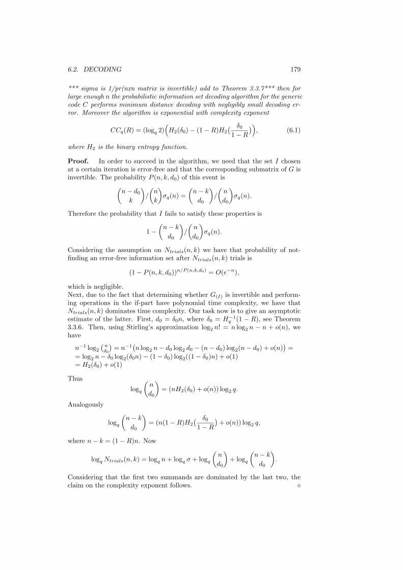
6.2. DECODING 179
*** sigma is 1/pr(nxn matrix is invertible) add to Theorem 3.3.7*** then forlarge enough n the probabilistic information set decoding algorithm for the genericcode C performs minimum distance decoding with negligibly small decoding er-ror. Moreover the algorithm is exponential with complexity exponent
CCq(R) = (logq 2)(H2(δ0)− (1−R)H2
( δ01−R
)), (6.1)
where H2 is the binary entropy function.
Proof. In order to succeed in the algorithm, we need that the set I chosenat a certain iteration is error-free and that the corresponding submatrix of G isinvertible. The probability P (n, k, d0) of this event is(
n− d0
k
)/
(n
k
)σq(n) =
(n− kd0
)/
(n
d0
)σq(n).
Therefore the probability that I fails to satisfy these properties is
1−(n− kd0
)/
(n
d0
)σq(n).
Considering the assumption on Ntrials(n, k) we have that probability of not-finding an error-free information set after Ntrials(n, k) trials is
(1− P (n, k, d0))n/P (n,k,d0) = O(e−n),
which is negligible.Next, due to the fact that determining whether G(I) is invertible and perform-ing operations in the if-part have polynomial time complexity, we have thatNtrials(n, k) dominates time complexity. Our task now is to give an asymptoticestimate of the latter. First, d0 = δ0n, where δ0 = H−1
q (1 − R), see Theorem3.3.6. Then, using Stirling’s approximation log2 n! = n log2 n − n + o(n), wehave
n−1 log2
(nd0
)= n−1
(n log2 n− d0 log2 d0 − (n− d0) log2(n− d0) + o(n)
)=
= log2 n− δ0 log2(δ0n)− (1− δ0) log2((1− δ0)n) + o(1)= H2(δ0) + o(1)
Thus
logq
(n
d0
)= (nH2(δ0) + o(n)) log2 q.
Analogously
logq
(n− kd0
)= (n(1−R)H2
( δ01−R
)+ o(n)) log2 q,
where n− k = (1−R)n. Now
logq Ntrials(n, k) = logq n+ logq σ + logq
(n
d0
)+ logq
(n− kd0
).
Considering that the first two summands are dominated by the last two, theclaim on the complexity exponent follows.
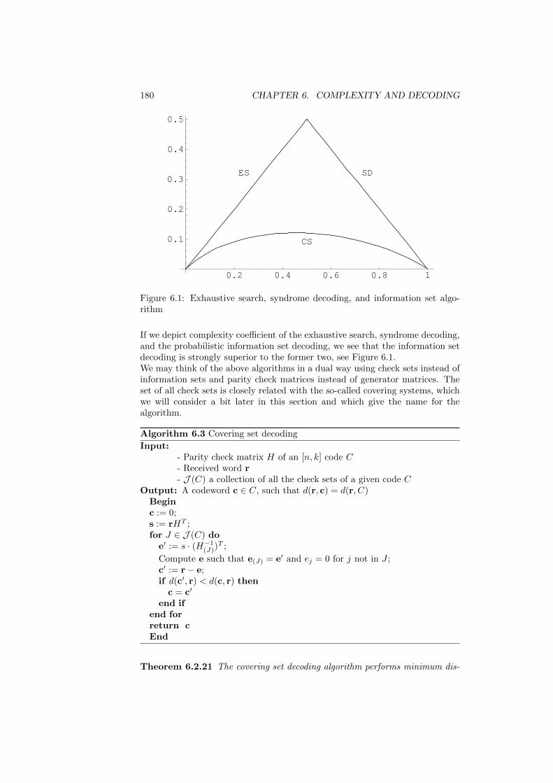
180 CHAPTER 6. COMPLEXITY AND DECODING
0.2 0.4 0.6 0.8 1
0.1
0.2
0.3
0.4
0.5
ES SD
CS
Figure 6.1: Exhaustive search, syndrome decoding, and information set algo-rithm
If we depict complexity coefficient of the exhaustive search, syndrome decoding,and the probabilistic information set decoding, we see that the information setdecoding is strongly superior to the former two, see Figure 6.1.We may think of the above algorithms in a dual way using check sets instead ofinformation sets and parity check matrices instead of generator matrices. Theset of all check sets is closely related with the so-called covering systems, whichwe will consider a bit later in this section and which give the name for thealgorithm.
Algorithm 6.3 Covering set decoding
Input:- Parity check matrix H of an [n, k] code C- Received word r- J (C) a collection of all the check sets of a given code C
Output: A codeword c ∈ C, such that d(r, c) = d(r, C)Beginc := 0;s := rHT ;for J ∈ J (C) do
e′ := s · (H−1(J))
T ;
Compute e such that e(J) = e′ and ej = 0 for j not in J ;c′ := r− e;if d(c′, r) < d(c, r) then
c = c′
end ifend forreturn cEnd
Theorem 6.2.21 The covering set decoding algorithm performs minimum dis-
6.2. DECODING 181
tance decoding.
Proof. Let r = c + e as in the proof of Theorem 6.2.19. From that proofwe know that there exists a check set J such that supp(e) ⊂ J . Now we haveHrT = HeT = H(J)e(J). Since for the check set J , the matrix H(J) is invertible,we may find e(J) and thus e.
Similarly to Algorithm 6.1 one may define the probabilistic version of the cov-ering set decoding. As we have already mentioned the covering set decodingalgorithm is closely related to the notion of a covering system. The overview ofthis notion follows next.
Definition 6.2.22 Let n, l and t be integers such that 0 < t ≤ l ≤ n. An(n, l, t) covering system is a collection J of subsets J of 1, . . . , n, such thatevery J ∈ J has l elements and every subset of 1, . . . , n of size t is containedin at least one J ∈ J . The elements J of a covering system J are also calledblocks. If a subset T of size t is contained in a J ∈ J , then we say that T iscovered or trapped by J .
Remark 6.2.23 From the proofs of Theorem 6.2.21 for almost all codes it isenough to find a a collection J of subsets J of 1, . . . , n, such that all J ∈ Jhave n − k elements and every subset of 1, . . . , n of size ρ = d0 + o(1) iscontained in at least one J ∈ J , thus obtaining (n, n− k, d0) covering system.
Example 6.2.24 The collection of all subsets of 1, . . . , n of size l is an (n, l, t)covering system for all 0 < t ≤ l. This collection consists of
(nl
)blocks.
Example 6.2.25 Consider F2q, the affine plane over Fq. Let n = q2 be the
number of its points. Then every line consists of q points, and every collectionof two points is covered by exactly one line. Hence there exists a (q2, q, 2)covering system. Every line that is not parallel to the x-axis is given by aunique equation y = mx + c. There are q2 of such lines. And there are q linesparallel to the y-axis. So the total number of lines is q2 + q.
Example 6.2.26 Consider the projective plane over Fq as treated in Section4.3.1. Let n = q2 + q + 1 be the number of its points. Then every line consistsof q+ 1 points, and every collection of two points is covered by exactly one line.There are q+ 1 lines. Hence there exists a (q2 + q+ 1, q+ 1, 2) covering systemconsisting of q + 1 blocks.
Remark 6.2.27 The number of blocks of an (n, l, t) covering system is consid-erably smaller than the number of all possible t-sets. It is still at least
(nt
)/(lt
).
But also this number grows exponentially in n if λ = limn→∞ l/n > 0 andτ = limn→∞ t/n > 0.
Definition 6.2.28 The covering coefficient b(n, l, t) is the smallest integer bsuch that there is an (n, l, t) covering system consisting of b blocks.
Although the exact value of the covering coefficient b(n, l, t) is an open problemwe do know its asymptotic logarithmic behavior.
182 CHAPTER 6. COMPLEXITY AND DECODING
Proposition 6.2.29 Let λ and τ be constants such that 0 < τ < λ < 1. Then
limn→∞
1
nlog b(n, bλnc, bτnc) = H2(τ)− λH2(τ/λ),
Proof. *** I suggest to skip the proof ***In order to establish this asymptotical result we prove lower and upper bounds,which are asymptotically identical. First the lower bound on b(n, l, t). Notethat every l-tuple traps
(lt
)t-tuples. Therefore, one needs at least(
n
t
)/
(l
t
)l-tuples. Now we use the relation from [?]: 2nH2(θ)−o+(n) ≤
(nθn
)≤ 2nH2(θ)
for 0 < θ < 1, where o+(n) is a non-negative function, such that o+(n) =o(n). Applying this lower bound for l = bλnc and t = bτnc we have
(nbτnc
)≥
2nH2(τ)−o+(n) and(bλncbτnc
)≤ 2nλH2(τ/λ). Therefore,
b(n, bλnc, bτnc) ≥(nbτnc
)/(bλncbτnc
)≥ 2n
(H2(τ)−λH2(τ/λ)
)+o+(n)
For a similar lower bound see Exercise ??.Now the upper bound. Consider a set S with f(n, l, t) independently and uni-formly randomly chosen l-tuples, such that
f(n, l, t) =
(nl
)(n−tn−l) · cn,
where c > ln 2. The probability that a t-tuple is not trapped by any tuple fromS is (
1−(n− tn− l
)/
(n
l
))f(n,l,t)
.
Indeed, the number of all l-tuples is(nl
), the probability of trapping a given t-
tuple T1 by an l-tuple T2 is the same as probability of trapping the complementof T2 by the complement of T1 and is equal to
(n−tn−l)/(nl
). The expected number
of non-trapped t-tuples is then(n
t
)(1−
(n− tn− l
)/
(n
l
))f(n,l,t)
.
Using the relation limx→∞(1− 1/x)x = e−1 and the expression for f(n, l, t) wehave that the expected number above tends to
T = 2nH2(t/n)+o(n)−cn log e
From the condition on c we have that T < 1. This implies that among allthe sets with f(n, l, t) independently and uniformly randomly chosen l-tuples,there exists one that traps all the t-tuples. Thus b(n, l, t) ≤ f(n, l, t). By thewell-known combinatorial identities(
n
t
)(n− tn− l
)=
(n
n− l
)(l
t
)=
(n
l
)(l
t
),
6.2. DECODING 183
we have that for t = bτnc and l = bλnc holds
b(n, l, t) ≤ 2n(H2(τ)−λH2(τ/λ)
)+o(n),
which asymptotically coincides with the lower bound proven above. Let us now turn to the case of bounded distance decoding. So here we are aimingat correcting some t errors, where t < ρ. The complexity result for almost allcodes is obtained by substituting t/n instead of δ0 in (6.1). In particular, fordecoding up to half the minimum distance for almost all codes we have thefollowing result.
Corollary 6.2.30 If Ntrials(n, k) is at least
n ·(
n
d0/2
)/
(n− kd0/2
),
then covering set decoding algorithm for almost all codes performs decoding upto half the minimum distance with negligibly small decoding error. Moreover thealgorithm is exponential with complexity coefficient
CSBq(R) = (logq 2)(H2(δ0/2)− (1−R)H2
( δ02(1−R)
)). (6.2)
We are interested now in bounded decoding up to t ≤ d − 1. For almost all(long) codes the case t = d− 1 coincides with the minimum distance decoding,see... . From Proposition 6.2.9 it is enough to find a collection J of subsetsJ of 1, . . . , n, such that all J ∈ J have d − 1 elements and every subsetof 1, . . . , n of size t is contained in at least one J ∈ J . Thus we need an(n, d− 1, t) covering system. Let us call this the erasure set decoding.
Example 6.2.31 Consider a code of length 13, dimension 9 and minimum dis-tance 5. The number of all 2-sets of 1, . . . , 13 is equal to
(132
)= 78. In order to
correct two errors one has to compute the linear combinations of two columns ofa parity check matrix H, for all the 78 choices of two columns, and see whetherit is equal to rHT for the received word r.An improvement can be obtained by a covering set. Consider the projectiveplane over F3 as in Example 6.2.26. Hence we have a (13, 4, 2) covering system.Using this covering system there are 13 subsets of 4 elements for which one hasto find HrT as a linear combination of the corresponding columns of the paritycheck matrix. So we have to consider 13 times a system of 4 linear equations in4 variables instead of 78 times a system of 4 linear equations in 2 variables.
From Proposition 6.2.29 and Remark ?? we have the complexity result for era-sure set decoding.
Proposition 6.2.32 Erasure set decoding performs bounded distance decodingfor every t = αδ0n, 0 < α ≤ 1. The algorithm is exponential with complexitycoefficient
ESq(R) = (logq 2)(H2(αδ0)− δ0H2(α)
). (6.3)
Proof. The proof is left to the reader as an exercise. It can be shown, see Exercise 6.2.7, that erasure set decoding is interior to cov-ering set for all α.
***Permutation decoding, Huffman-Pless 10.2, ex Golay q=3, exer q=2***
184 CHAPTER 6. COMPLEXITY AND DECODING
6.2.4 Nearest neighbor decoding
***decoding using minimal codewords.
6.2.5 Exercises
6.2.1 Count an erasure as half an error. Use this idea to define an extensionof the Hamming distance on (Fq ∪ ?)n and show that it is a metric.
6.2.2 Give a proof of Proposition 6.2.8.
6.2.3 Consider the code C over F11 with parameters [11, 7, 5] of Example6.2.13. Suppose that we receive the word (7, 6, 5, 4, 3, 2, 1, ?, ?, ?, ?) with 4 era-sures and no errors. Which codeword is sent?
6.2.4 Consider the code C1 over F11 with parameters [11, 4, 8] of Example6.2.13. Suppose that we receive the word (4, 3, 2, 1, ?, ?, ?, ?, ?, ?, ?) with 7 era-sures and no errors. Find the codeword sent.
6.2.5 Consider the covering systems of lines in the affine space Fmq of dimensionm over Fq, and the projective space of dimension m over Fq, respectively. Showthe existence of a (qn, q, 2) and a ((qm+1 − 1)/(q − 1), q + 1, 2) covering systemas in Examples 6.2.25 and 6.2.26 in the case m = 2. Compute the number oflines in both cases.
6.2.6 Prove the following lower bound on b(n, l, t):
b(n, l, t) ≥⌈nl
⌈n− 1
l − 1. . .⌈n− t+ 1
l − t+ 1
⌉. . .⌉⌉.
Hint : By double counting argument prove first that l · b(n, l, t) ≥ n · b(n− 1, l−1, t− 1) and then use b(n, l, 1) = dn/le.
6.2.7 By using the properties of binary entropy function prove that for all0 < R < 1 and 0 < α < 1 holds
(1−R)H2
(αH−1q (1−R)
1−R
)> H−1
q (1−R) ·H2(α).
Conclude that covering set decoding is superior to erasure set.
6.3 Difficult problems in coding theory
6.3.1 General decoding and computing minimum distance
We have formulated the decoding problem in Section 6.2. As we have seen thatthe minimum (Hamming) distance of a linear code is an important parameterwhich can be used to estimate the decoding performance. However, a largerminimum distance does not guarantee the existence of an efficient decoding al-gorithm. It is natural to ask the following computational questions: For generallinear codes, whether there exists a decoding algorithm with polynomial-timecomplexity? Whether or not there exists a polynomial-time algorithm whichfinds the minimum distance for any linear code? It has been proved that these
6.3. DIFFICULT PROBLEMS IN CODING THEORY 185
computational problems are both intractable.
Let C be an [n, k] binary linear code. Suppose r is the received word. Accordingto the maximum-likelihood decoding principle, we wish to find a codeword suchthat the Hamming distance between r and the codeword is minimal. As wehave seen in previous sections that using the brute force search, correct decod-ing requires 2k comparisons in the worst case, and thus has exponential-timecomplexity.
Consider the syndrome of the received word. Let H be a parity-check matrix ofC, which is an m×n matrix, where m = n− k. The syndrome of r is s = rHT .The following two computational problems are equivalent, letting c = r− e:
(1) (Maximum-likelihood decoding problem) Finding a codeword c suchthat d(r, c) is minimal.
(2) Finding a minimum-weight solution e to the equation xHT = s.
Clearly, an algorithm which solves the following computational problem (3) alsosolves the above Problem (2).
(3) For any non-negative integer w, find a vector x of Hamming weight ≤ wsuch that xHT = s.
Conversely, an algorithm which solves Problem (2) must solve Problem (3). Infact, suppose e is a minimum-weight solution e to the equation xHT = s. Then,for w < wt(e), the algorithm will return “no solution”; for w ≥ wt(e), the algo-rithm returns e. Thus, the maximum-likelihood decoding problem is equivalentthe above problem (3).
The decision problem of the maximum-likelihood decoding problem is as
Decision Problem of Decoding Linear Codes
INSTANCE: An m× n binary matrix H, a binary vector s of length m, anda non-negative integer w.
QUESTION: Is there a binary vector x ∈ Fn2 of Hamming weight ≤ w suchthat xHT = s?
Proposition 6.3.1 The decision problem of decoding linear codes is an NP-complete problem.
We will prove this proposition by reducing the three-dimensional matching prob-lem to the decision problem of decoding linear codes. The three-dimensionalmatching problem is a well-known NP-complete problem. For the completeness,we recall this problem as follows.
Three-Dimensional Matching Problem
INSTANCE: A set T ⊆ S1 × S2 × S3, where S1, S2, and S3 are disjoint finitesets having same number of elements, a = |S1| = |S2| = |S3|.
186 CHAPTER 6. COMPLEXITY AND DECODING
QUESTION: Does T contain a matching, that is, a subset U ⊆ T such that|U | = a and no two elements of U agree in any coordinate?
We now construct a matrix M which is called the incidence matrix of T asfollows. Fix an ordering of the triples of T . Let ti = (ti1, ti2, ti3) denote thei-th triple of T for i = 1, . . . , |T |. The matrix M has |T | rows and 3a columns.Each row mi of M is a binary vector of length 3a and Hamming weight 3,which is constituted of three blocks bi1, bi2 and bi3, of the same length a, i.e.,mi = (bi1,bi2,bi3). For u = 1, 2, 3, if tiu is the v element of Su, then the v-thcoordinate of biu is 1, all the other coordinates of this block is 0.
Clearly, the existence of a matching of the Three-Dimensional Matching Prob-lem is equivalent to the existence of a rows of M such that their mod 2 sum is
(1, 1, . . . , 1), that is, there exist a binary vector x ∈ F|T |2 of weight a such thatxM = (1, 1, . . . , 1) ∈ F3a
2 . Now we are ready to prove Proposition 6.3.1.
Proof of Proposition 6.3.1. Suppose we have a polynomial-time algorithmsolving the Decision Problem of Decoding Linear Codes. Given an input T ⊆S1 × S2 × S3 for the Three-Dimensional Matching Problem, set H = MT ,where M is the incidence matrix of T , s = (1, 1, . . . , 1) and w = a. Then run-ning the algorithm for the Decision Problem of Decoding Linear Codes, we willdiscover whether or not there exist the desired matching. Thus, a polynomial-time algorithm for the Decision Problem of Decoding Linear Codes implies apolynomial-time algorithm for the Three-Dimensional Matching Problem. Thisproves the Decision Problem of Decoding Linear Codes is NP-complete.
Next, let us the consider the problem of computing the minimum distance of an[n, k] binary linear code C with a parity-check matrix H. For any linear code,the minimum distance is equal to the minimum weight, we use these two termsinterchangeably. Consider the following decision problem.
Decision Problem of Computing Minimum Distance
INSTANCE: An m× n binary matrix H and a non-negative integer w.
QUESTION: Is there a nonzero binary vector x of Hamming weight w suchthat xHT = 0?
If we have an algorithm which solves the above problem, then we can run thealgorithm with w = 1, 2, . . ., and the first integer d with affirmative answer isthe minimum weight of C. On the other hand, if we have an algorithm whichfinds the minimum weight d of C, then we can solve the above problem bycomparing w with d. Therefore, we call this problem the Decision Problemof Computing Minimum Distance, and the NP-completeness of this problemimplies the NP-hardness of the problem of computing the minimum distance.
6.3. DIFFICULT PROBLEMS IN CODING THEORY 187
***Computing the minimum distance:– brute force, complexity (qk − 1)/(q − 1), O(qk)– minimal number of parity checks: O(
(nk
)k3)***
***Brouwer’s algorithm and variations, Zimmerman-Canteau-Chabeaud, Sala***
*** Vardy’s result: computing the min. dist. is NP hard***
6.3.2 Is decoding up to half the minimum distance hard?
Finding the minimum distance and decoding up to half the minimum distanceare closely related problems.
Algorithm 6.3.2 Suppose that A is an algorithm that computes the minimumdistance of an Fq-linear code C that is given by a parity check matrix H. Wedefine an algorithm D with input y ∈ Fnq . Let s = HyT be the syndrome of
y with respect to H. Let H = [H|s] be the parity check matrix of the codeC of length n + 1. Let Ci be the code that is obtained by puncturing C atthe i-th position. Use algorithm A to compute d(C) and d(Ci) for i ≤ n. Lett = mind(Ci)|i ≤ n. Let I = i|t = d(Ci), i ≤ n. Assume |I| = t andt < d(C). Assume furthermore that erasure decoding at the positions I finds aunique codeword c in C such that ci = yi for all i not in I. Output c in casethe above assumptions are met, and output ∗ otherwise.
Proposition 6.3.3 Let A be an algorithm that computes the minimum dis-tance. Let D be the algorithm that is defined in 6.3.2. Let y ∈ Fnq be an input.Then D is a decoder that gives as output c in case d(C,y) < d(C) and y has cas unique nearest codeword. In particular D is a decoder of C that corrects upto half the minimum distance.
Proof. Let y be a word with t = d(C,y) < d(C) and suppose that c is aunique nearest codeword. Then y = c + e with c ∈ C and t = wt(e). Note that(e,−1) ∈ C, since s = HyT = HeT . So d(C) ≤ t+1. Let z be in C. If zn+1 = 0,then z = (z, 0) with z ∈ C. Hence wt(z) ≥ d(C) ≥ t + 1. If zn+1 6= 0, thenwithout loss of generality we may assume that z = (z,−1). So H zT = 0. HenceHzT = s. So c′ = y − z ∈ C. If wt(z) ≤ t+ 1, then wt(z) ≤ t. So d(y, c′) ≤ t.Hence c′ = c, since c is the unique nearest codeword by assumption. Thereforez = e and wt(z) = t. Hence d(C) = t+ 1, since t+ 1 ≤ d(C).Let Ci be the code that is obtained by puncturing C at the i-th position. Usethe algorithm A to compute d(Ci) for all i ≤ n. An argument similar to aboveshows that d(Ci) = t if i is in the support of e, and d(Ci) = t+ 1 if i is not inthe support of e. So t = mind(Ci)|i ≤ n and I = i|t = d(Ci), i ≤ n is thesupport of e and has size t. So the error positions are known. Computing theerror values is matter of linear algebra as shown in Proposition 6.2.11. In thisway e and c are found.
Proposition 6.3.4 Let MD be the problem of computing the minimum distanceof a code given by a parity check matrix. Let DHMD be the problem of decodingup to half the minimum distance. Then
DHMD ≤P MD.
188 CHAPTER 6. COMPLEXITY AND DECODING
Proof. Let A be an algorithm that computes the minimum distance of an Fq-linear code C that is given by a parity check matrix H. Let D be the algorithmgiven in 6.3.2. Then A is used (n+ 1)-times in D. Suppose that the complexityof A is polynomial of degree e. We may assume that e ≥ 2. Computing theerror values can be done with complexity O(n3) by Proposition 6.2.11. Thenthe complexity of D is polynomial of degree e+ 1.
***Sendrier and Finasz******Decoding with preprocessing, Bruck-Naor***
6.3.3 Other hard problems
***worse case versus average case, the simplex method for linear programming isan example of an algorithm that runs almost always fast, that is polynomially inits input, but for which is known to be exponentially in the worst case. Ellipsoidmethod, Khachian’s method***
***approximate solutions of NP-hard problems***
6.4 Notes
In 1978, Berlekamp, McEliece and van Tilborg proved that the maximum-likelihood decoding problem is NP-hard for general binary codes. Vardy showedin 1997 that the problem of computing the minimum distance of a binary linearcode is NP-hard.
Chapter 7
Cyclic codes
Ruud Pellikaan
Cyclic codes have been in the center of interest in the theory of error-correctingcodes since their introduction. Cyclic codes of relatively small length have goodparameters. In the list of 62 binary cyclic codes of length 63 there are 51 codesthat have the largest known minimum distance for a given dimension amongall linear codes of length 63. Binary cyclic codes are better than the Gilbert-Varshamov bound for lengths up to 1023. Although some negative results areknown indicating that cyclic codes are asymptotically bad, this still is an openproblem. Rich combinatorics is involved in the determination of the parametersof cyclic codes in terms of patterns of the defining set.
***...***
7.1 Cyclic codes
7.1.1 Definition of cyclic codes
Definition 7.1.1 The cyclic shift σ(c) of a word c = (c0, c1, . . . , cn−1) ∈ Fnq isdefined by
σ(c) := (cn−1, c0, c1, . . . , cn−2).
An Fq-linear code C of length n is called cyclic if
σ(c) ∈ C for all c ∈ C.
The subspaces 0 and Fnq are clearly cyclic and are called the trivial cycliccodes.
Remark 7.1.2 In the context of cyclic codes it is convenient to consider theindex i of a word modulo n and the convention is that the numbering of elements(c0, c1, . . . , cn−1) starts with 0 instead of 1. The cyclic shift defines a linear mapσ : Fnq → Fnq . The i-fold composition σi = σ · · · σ is the i-fold forward shift.Now σn is the identity map and σn−1 is the backward shift. A cyclic code isinvariant under σi for all i.
189
190 CHAPTER 7. CYCLIC CODES
Proposition 7.1.3 Let G be a generator matrix of a linear code C. Then C iscyclic if and only if the cyclic shift of every row of G is in C.
Proof. If C is cyclic, then the cyclic shift of every row of G is in C, since allthe rows of G are codewords.Conversely, suppose that the cyclic shift of every row of G is in C. Let g1, . . . ,gkbe the rows of G. Let c ∈ C. Then c =
∑ki=1 xigi for some x1, . . . , xk ∈ Fq.
Now σ is a linear transformation of Fnq . So
σ(c) =
k∑i=1
xiσ(gi) ∈ C,
since C is linear and σ(gi) ∈ C for all i by assumption. Hence C is cyclic.
Example 7.1.4 Consider the [6,3] code over F7 with generator matrix G de-fined by
G =
1 1 1 1 1 11 3 2 6 4 51 2 4 1 2 4
.
Then σ(g1) = g1, σ(g2) = 5g2 and σ(g3) = 4g3. Hence the code is cyclic.
Example 7.1.5 Consider the [7, 4, 3] Hamming code C, with generator matrixG as given in Example 2.2.14. Then (0, 0, 0, 1, 0, 1, 1), the cyclic shift of thethird row is not a codeword. Hence this code is not cyclic. After a permutationof the columns and rows of G we get the generator matrix G′ of the code C ′,where
G′ =
1 0 0 0 1 1 00 1 0 0 0 1 10 0 1 0 1 1 10 0 0 1 1 0 1
.
Let g′i be the i-th row of G′. Then σ(g′1) = g′2, σ(g′2) = g′1 +g′3, σ(g′3) = g′1 +g′4and σ(g′4) = g′1. Hence C ′ is cyclic by Proposition 7.1.3. Therefore C is notcyclic, but equivalent to a cyclic code C ′.
Proposition 7.1.6 The dual of a cyclic code is again cyclic.
Proof. Let C be a cyclic code. Then σ(c) ∈ C for all c ∈ C. So
σn−1(c) = (c1, . . . , cn−1, c0) ∈ C for all c ∈ C.
Let x ∈ C⊥. Then
σ(x) · c = xn−1c0 + x0c1 + · · ·+ xn−2cn−1 = x · σn−1(c) = 0
for all c ∈ C. Hence C⊥ is cyclic.
7.1. CYCLIC CODES 191
7.1.2 Cyclic codes as ideals
The set of all polynomials in the variable X with coefficients in Fq is denotedby Fq[X]. Two polynomials can be added and multiplied and in this way Fq[X]is a ring. One has division with rest this means that very polynomial f(X) hasafter division with another nonzero polynomial g(X) a quotient q(X) with restr(X) that is zero or of degree strictly smaller than deg g(X). In other words
f(X) = q(X)g(X) + r(X) and r(X) = 0 or deg r(X) < deg g(X).
In this way Fq[X] with its degree is a Euclidean domain. Using division withrest repeatedly we find the greatest common divisor gcd(f(X), g(X)) of twopolynomials f(X) and g(X) by the algorithm of Euclid.***complexity of Euclidean Algorithm***
Every nonempty subset of a ring that is closed under addition and multiplicationby an arbitrary element of the the ring is called an ideal. Let g1, . . . , gm be givenelements of a ring. The set of all a1g1 + · · ·+ amgm with a1, . . . , am in the ring,forms an ideal and is denoted by 〈g1, . . . , gm〉 and is called the ideal generatedby g1, . . . , gm. As a consequence of division with rest every ideal in Fq[X] iseither 0 or generated by a one unique monic polynomial. Furthermore
〈f(X), g(X)〉 = 〈gcd(f(X), g(X))〉.
We refer for these notions and properties to Appendix ??.
Definition 7.1.7 Let R be a ring and I an ideal in R. Then R/I is the factorring of R modulo I. If R = Fq[X] and I = 〈Xn − 1〉 is the ideal generated byXn − 1, then Cq,n is the factor ring
Cq,n = Fq[X]/〈Xn − 1〉.
Remark 7.1.8 The factor ring Cq,n has an easy description. Every polynomialf(X) has after division by Xn − 1 a rest r(X) of degree at most n− 1, that isthere exist polynomials q(X) and r(X) such that
f(X) = q(X)(Xn − 1) + r(X) and deg r(X) < n or r(X) = 0.
The coset of the polynomial f(X) modulo Xn − 1 is denoted by f(x). Hencef(X) and r(X) have the same coset and represent the same element in Cq,n.Now xi denotes the coset of Xi modulo 〈Xn−1〉. Hence the cosets 1, x, . . . , xn−1
form a basis of Cq,n over Fq. The multiplication of the basis elements xi and xj
in Cq,n with 0 ≤ i, j < n is given by
xixj =
xi+j if i+ j < n,xi+j−n if i+ j ≥ n,
Definition 7.1.9 Consider the map ϕ between Fnq and Cq,n
ϕ(c) = c0 + c1x+ · · ·+ cn−1xn−1.
Then ϕ(c) is also denoted by c(x).
192 CHAPTER 7. CYCLIC CODES
Proposition 7.1.10 The map ϕ is an isomorphism of vector spaces. Ideals inthe ring Cq,n correspond one-to-one to cyclic codes in Fnq .
Proof. The map ϕ is clearly linear and it maps the i-th standard basis vectorof Fnq to the coset xi−1 in Cq,n for i = 1, . . . , n. Hence ϕ is an isomorphism ofvector spaces. Let ψ be the inverse map of ϕ.Let I be an ideal in Cq,n. Let C := ψ(I). Then C is a linear code, since ψ is alinear map. Let c ∈ C. Then c(x) = ϕ(c) ∈ I and I is an ideal. So xc(x) ∈ I.But
xc(x) = c0x+c1x2+· · ·+cn−2x
n−1+cn−1xn = cn−1+c0x+c1x
2+· · ·+cn−2xn−1,
since xn = 1. So ψ(xc(x)) = (cn−1, c0, c1 . . . , cn−2) ∈ C. Hence C is cyclic.Conversely, let C be a cyclic code in Fnq , and let I := ϕ(C). Then I is closedunder addition of its elements, since C is a linear code and ϕ is a linear map.If a ∈ Fnq and c ∈ C, then
a(x)c(x) = ϕ(a0c + a1σ(c) + · · ·+ an−1σn−1(c)) ∈ I.
Hence I is an ideal in Cq,n.
In the following we will not distinguish between words and the correspondingpolynomials under ϕ; we will talk about words c(x) when in fact we mean thevector c and vice versa.
Example 7.1.11 Consider the rows of the generator matrix G′ of the [7, 4, 3]Hamming code of Example 7.1.5. They correspond to g′1(x) = 1 + x4 + x5,g′2(x) = x + x5 + x6, g′3(x) = x2 + x4 + x5 + x6 and g′4(x) = x3 + x4 + x6,respectively. Furthermore x·x6 = 1, so x is invertible in the ring F2[X]/〈X7−1〉.Now
〈1 + x4 + x5〉 = 〈x+ x5 + x6〉 = 〈x6 + x10 + x11〉 = 〈x3 + x4 + x6〉.
Hence the ideals generated by g′i(x) are the same for i = 1, 2, 4 and there is nounique generating element. The third row generates the ideal
〈x2+x4+x5+x6〉 = 〈x2(1+x2+x3+x4)〉 = 〈1+x2+x3+x4〉 = 〈(1+x)(1+x+x3)〉,
which gives a cyclic code that is a proper subcode of dimension 3. Therefore allexcept the third element generate the same ideal.
7.1.3 Generator polynomial
Remark 7.1.12 The ring Fq[X] with its degree function is an Euclidean ring.Hence Fq[X] is a principal ideal domain, that means that all ideals are generatedby one element. If an ideal of Fq[X] is not zero, then a generating elementis unique up to a nonzero scalar multiple of Fq. So there is a unique monicpolynomial generating the ideal. Now Cq,n is a factor ring of Fq[X], therefore itis also a principal ideal domain. A cyclic code C considered as an ideal in Cq,nis generated by one element, but this element is not unique, as we have seen inExample 7.1.11. The inverse image of C under the map Fq[X]→ Cq,n is denoted
7.1. CYCLIC CODES 193
by I. Then I is a nonzero ideal in Fq[X] containing Xn − 1. Therefore I has aunique monic polynomial g(X) as generator. So g(X) is the monic polynomialin I of minimal degree. Hence g(X) is the monic polynomial of minimal degreesuch that g(x) ∈ C.
Definition 7.1.13 Let C be a cyclic code. Let g(X) be the monic polynomialof minimal degree such that g(x) ∈ C. Then g(X) is called the generatorpolynomial of C.
Example 7.1.14 The generator polynomial of the trivial code Fnq is 1, and ofthe zero code of length n is Xn − 1. The repetition code and its dual have asgenerator polynomials Xn−1 + · · ·+X + 1 and X − 1, respectively.
Proposition 7.1.15 Let g(X) be a polynomial in Fq[X]. Then g(X) is a gen-erator polynomial of a cyclic code over Fq of length n if and only if g(X) ismonic and divides Xn − 1.
Proof. Suppose g(X) is the generator polynomial of a cyclic code. Then g(X)is monic and a generator of an ideal in Fq[X] that contains Xn−1. Hence g(X)divides Xn − 1.Conversely, suppose that g(X) is monic and divides Xn − 1. So b(X)g(X) =Xn − 1 for some b(X). Now 〈g(x)〉 is an ideal in Cq,n and defines a cyclic codeC. Let c(X) be a monic polynomial such that c(x) ∈ C. Then c(x) = a(x)g(x).Hence there exists an h(X) such that
c(X) = a(X)g(X) + h(X)(Xn − 1) = (a(X) + b(X)h(X))g(X)
Hence deg g(X) ≤ deg c(X). Therefore g(X) is the monic polynomial of minimaldegree such that g(x) ∈ C. Hence g(X) is the generator polynomial of C.
Example 7.1.16 The polynomial X3 +X + 1 divides X8 − 1 in F3[X], since
(X3 +X + 1)(X5 −X3 −X2 +X − 1) = X8 − 1.
Hence 1 +X +X3 is a generator polynomial of a ternary cyclic code of length8.
Remark 7.1.17 Let g(X) be the generator polynomial of C. Then g(X) is amonic polynomial and g(x) generates C. Let c(X) be another polynomial suchthat c(x) generates C. Let d(X) be the greatest common divisor of c(X) andXn − 1. Then d(X) is the monic polynomial such that
〈d(X)〉 = 〈c(X), Xn − 1〉 = I.
But also g(X) is the unique monic polynomial such that 〈g(X)〉 = I. Henceg(X) = gcd(c(X), Xn − 1).
Example 7.1.18 Consider the binary cyclic code of length 7 and generated by1 + x2. Then 1 +X2 = (1 +X)2 and 1 +X7 is divisible by 1 +X in F2[X]. So1 +X is the the greatest common divisor of 1 +X7 and 1 +X2. Hence 1 +Xis the generator polynomial of C.
194 CHAPTER 7. CYCLIC CODES
Example 7.1.19 Let C be the Hamming code of Examples 7.1.5 and 7.1.11.Then 1 + x4 + x5 generates C. In order to get the greatest common divisor of1 +X7 and 1 +X4 +X5 we apply the Euclidean algorithm:
1 +X7 = (1 +X +X2)(1 +X4 +X5) + (X +X2 +X4),
1 +X4 +X5 = (1 +X)(X +X2 +X4) + (1 +X +X3),
X +X2 +X4 = X(1 +X +X3).
Hence 1 +X +X3 is the greatest common divisor, and therefore 1 +X +X3 isthe generator polynomial of C.
Remark 7.1.20 Let g(X) be a generator polynomial of a cyclic code of lengthn, then g(X) divides Xn − 1 by Proposition 7.1.15. So g(X)h(X) = Xn − 1 forsome h(X). Hence g(0)h(0) = −1. Therefore the constant term of the generatorpolynomial of a cyclic code is not zero.
Proposition 7.1.21 Let g(X) = g0+g1X+· · ·+glX l be a polynomial of degreel. Let n be an integer such that l ≤ n. Let k = n− l. Let G be the k× n matrixdefined by
G =
g0 g1 · · · gl 0 · · · 0
0 g0 g1 · · · gl. . .
......
. . .. . .
. . . · · ·. . . 0
0 · · · 0 g0 g1 · · · gl
.
1. If g(X) is the generator polynomial of a cyclic code C, then the dimensionof C is equal to k and a generator matrix of C is G.
2. If gl = 1 and G is the generator matrix of a code C such that
(gl, 0, · · · , 0, g0, g1, · · · , gl−1) ∈ C,
then C is cyclic with generator polynomial g(X).
Proof.1) Suppose g(X) is the generator polynomial of a cyclic code C. Then theelement g(x) generates C and the elements g(x), xg(x), . . . , xk−1g(x) correspondto the rows of the above matrix.The generator polynomial is monic, so gl = 1 and the k × k submatrix of Gconsisting of the last k columns is a lower diagonal matrix with ones on thediagonal, so the rows of G are independent. Every codeword c(x) ∈ C is equalto a(x)g(x) for some a(X). Division with remainder of Xn − 1 by a(X)g(X)gives that there exist e(X) and f(X) such that
a(X)g(X) = e(X)(Xn − 1) + f(X) and deg f(X) < n or f(X) = 0.
But Xn − 1 is divisible by g(X) by Proposition 7.1.15. So f(X) is divisible byg(X). Hence f(X) = b(X)g(X) and deg b(X) < n− l = k or b(X) = 0 for somepolynomial b(X). Therefore c(x) = a(x)g(x) = b(x)g(x) and deg b(X) < k orb(X) = 0. So every codeword is a linear combination of g(x), xg(x), . . . , xk−1g(x).
7.1. CYCLIC CODES 195
Hence k is the dimension of C and G is a generator matrix of C.2) Suppose G is the generator matrix of a code C such that gl = 1 and
(gl, 0, · · · , 0, g0, g1, · · · , gl−1) ∈ C.
Then the cyclic shift of the i-th row of G is the (i+ 1)-th row of G for all i < k,and the cyclic shift of the k-th row of G is (gl, 0, · · · , 0, g0, g1, · · · , gl−1) whichis also an element of C by assumption. Hence C is cyclic by Proposition 7.1.3.Now gl = 1 and the upper right corner of G consists of zeros, so G has rankk and the dimension of C is k. Now g(X) is monic, has degree l = n − k andg(x) ∈ C. The generator polynomial of C has the same degree l by (1). Henceg(X) is the generator polynomial of C.
Example 7.1.22 The ternary cyclic code of length 8 with generator polynomial1 +X +X3 of Example 7.1.16 has dimension 5.
Remark 7.1.23 A cyclic [n, k] code is systematic at the first k positions, sinceit has a generator matrix as given in Proposition 7.1.21 which is upper diagonalwith nonzero entries on the diagonal at the first k positions, since g0 6= 0 byRemark 7.1.20. So the row reduced echelon form of a generator matrix ofthe code has the k × k identity matrix at the first k columns. The last rowof this rref matrix is up to the constant g0 equal to (0, · · · , 0, g0, g1, · · · , gl)giving the coefficients of the generator polynomial. This methods of obtainingthe generator polynomial out of a given generator matrix G is more efficientthan taking the greatest common divisor of g1(X), . . . , gk(X), Xn − 1, whereg1, . . . ,gk are the rows of G.
Example 7.1.24 Consider generator matrix G of the [6,3] cyclic code over F7
of Example 7.1.4. The row reduced echelon form of G is equal to 1 0 0 6 1 30 1 0 3 3 60 0 1 6 4 6
.
The last row represents
x2 + 6x3 + 4x4 + 6x5 = x2(1 + 6x+ 4x2 + 6x3)
Hence 1 + 6x+ 4x2 + 6x3 is a codeword. The corresponding monic polynomial6 +X + 3X2 +X3 has degree 3. Hence this is the generator polynomial.
7.1.4 Encoding cyclic codes
Consider a cyclic code of length n with generator polynomial g(X) and thecorresponding generator matrix G as in Proposition 7.1.21. Let the messagem = (m0, . . . ,mk−1) ∈ Fkq be mapped to the codeword c = mG. In terms ofpolynomials that means that
c(x) = m(x)g(x), where m(x) = m0 + · · ·+mk−1xk−1.
In this way we get an encoding of message words into codewords.The k × k submatrix of G consisting of the last k columns of G is a lower
196 CHAPTER 7. CYCLIC CODES
triangular matrix with ones on its diagonal, so it is invertible. That means thatwe can perform row operations on this matrix until we get another matrix G2
such that its last k columns form the k × k identity matrix. The matrix G2 isanother generator matrix of the same code. The encoding
m 7→ c2 = mG2
by means of G2 is systematic in the last k positions, that means that there existr0, . . . , rn−k−1 ∈ Fq such that
c2 = (r0, . . . , rn−k−1,m0, . . . ,mk−1).
In other words the encoding has the nice property, that one can read off thesent message directly from the encoded word by looking at the last k positions,in case no errors appeared during the transmission at these positions.Now how does one translate this systematic encoding in terms of polynomials?Let m(X) be a polynomial of degree at most k− 1. Let −r(X) be the rest afterdividing m(X)Xn−k by g(X). Now deg(g(X)) = n−k. So there is a polynomialq(X) such that
m(X)Xn−k = q(X)g(X)− r(X) and deg(r(X)) < n− k or r(X) = 0.
Hence r(x) +m(x)xn−k = q(x)g(x) is a codeword of the form
r0 + r1x+ · · ·+ rn−k−1xn−k−1 +m0x
n−k + · · ·+mk−1xn−1.
Example 7.1.25 Consider the cyclic [7,4,3] Hamming code of Example 7.1.19with generator polynomial g(X) = 1 + X + X3. Let m be a message withpolynomial m(X) = 1 + X2 + X3. Then division of m(X)X3 by g(X) givesas quotient q(X) = 1 + X + X2 + X3 with rest r(X) = 1. The correspondingcodeword by systematic encoding is
c2(x) = r(x) +m(x)x3 = 1 + x3 + x5 + x6.
Example 7.1.26 Consider the ternary cyclic code of length 8 with generatorpolynomial 1+X+X3 of Example 7.1.16. Let m be a message with polynomialm(X) = 1 + X2 + X3. Then division of m(X)X3 by g(X) gives as quotientq(X) = −1 − X + X2 + X3 with rest −r(X) = 1 − X. The correspondingcodeword by systematic encoding is
c2(x) = r(x) +m(x)x3 = −1 + x+ x3 + x5 + x6.
7.1.5 Reversible codes
Definition 7.1.27 Define the reversed word ρ(x) of x ∈ Fnq by
ρ(x0, x1, . . . , xn−2, xn−1) = (xn−1, xn−2, . . . , x1, x0).
Let C be a code in Fnq , then its reversed code ρ(C) is defined by
ρ(C) = ρ(c) | c ∈ C .
A code is called reversible if C = ρ(C).
7.1. CYCLIC CODES 197
Remark 7.1.28 The dimensions of C and ρ(C) are the same, since ρ is anautomorphism of Fnq . If a code is reversible, then ρ ∈ Aut(C).
Definition 7.1.29 Let g(X) be a polynomial of degree l given by
g0 + g1X + · · ·+ gl−1Xl−1 + glX
l.
Then
X lg(X−1) = gl + gl−1X + · · ·+ g1Xl−1 + g0X
l.
is called the reciprocal of g(X). If moreover g(0) 6= 0, then X lg(X−1)/g(0) iscalled the monic reciprocal of g(X). The polynomial g(X) is called reversible ifg(0) 6= 0 and it is equal to its monic reciprocal.
Remark 7.1.30 If g = (g0, g1, . . . , gl−1, gl) are the coefficients of the polyno-mial g(X), then the reversed word ρ(g) give the coefficients of the reciprocal ofg(X).
Remark 7.1.31 If α is a zero of g(X) and α 6= 0, then the reciprocal α−1 is azero of the reciprocal of g(X).
Proposition 7.1.32 Let g(X) be the generator polynomial of a cyclic code C.Then ρ(C) is cyclic with the monic reciprocal of g(X) as generator polynomial,and C is reversible if and only if g(X) is reversible.
Proof. A cyclic code is invariant under the forward shift σ and the backwardshift σn−1. Now σ(ρ(c)) = ρ(σn−1(c)) for all c ∈ C. Hence ρ(C) is cyclic.Now g(0) 6= 0 by Remark 7.1.20. Hence the monic reciprocal of g(X) is welldefined and its corresponding word is an element of ρ(C) by Remark 7.1.30. Thedegree of g(X) and its monic reciprocal are the same, and the dimensions of Cand ρ(C) are the same. Hence this monic reciprocal is the generator polynomialof ρ(C).Therefore C is reversible if and only if g(X) is reversible, by the definition of areversible polynomial.
Remark 7.1.33 If C is a reversible cyclic code, then the group generated byσ and ρ is the dihedral group of order 2n and is contained in Aut(C).
7.1.6 Parity check polynomial
Definition 7.1.34 Let g(X) be the generator polynomial of a cyclic code C oflength n. Then g(X) divides Xn − 1 by Proposition 7.1.15 and
h(X) =Xn − 1
g(X)
is called the parity check polynomial of C.
Proposition 7.1.35 Let h(X) be the parity check polynomial of a cyclic codeC. Then c(x) ∈ C if and only if c(x)h(x) = 0.
198 CHAPTER 7. CYCLIC CODES
Proof. Let c(x) ∈ C. Then c(x) = a(x)g(x), for some a(x). We have thatg(X)h(X) = Xn − 1. Hence g(x)h(x) = 0. So c(x)h(x) = a(x)g(x)h(x) = 0.Conversely, suppose that c(x)h(x) = 0. There exist polynomials a(X) and b(X)such that
c(X) = a(X)g(X) + b(X) and b(X) = 0 or deg b(X) < deg g(X).
Hencec(x)h(x) = a(x)g(x)h(x) + b(x)h(x) = b(x)h(x).
Notice that b(x)h(x) 6= 0 if b(X) is a nonzero polynomial, since deg b(X)h(X)is at most n− 1. Hence b(X) = 0 and c(x) = a(x)g(x) ∈ C.
Remark 7.1.36 If H is a parity check matrix for a code C, then H is a gen-erator matrix for the dual of C. One might expect that if h(X) is the paritycheck polynomial for a cyclic code C, then h(X) is the generator polynomial ofthe dual of C. This is not the case but something of this nature is true as thefollowing shows.
Proposition 7.1.37 Let h(X) be the parity check polynomial of a cyclic codeC. Then the monic reciprocal of h(X) is the generator polynomial of C⊥.
Proof. Let C be a cyclic code of length n and dimension k with generatorpolynomial g(X) and parity check polynomial h(X).If k = 0, then g(X) = Xn − 1 and h(X) = 1 and similarly if k = n, theng(X) = 1 and h(X) = Xn − 1. Hence the proposition is true in these cases.Now suppose that 0 < k < n. Then h(X) = h0 + h1X + · · ·+ hkX
k. Hence
Xkh(X−1) = hk + hk−1X + · · ·+ h0Xk.
The i-th position of xkh(x−1) is hk−i. Let g(X) be the generator polynomial ofC. Let l = n− k. Then g(X) = g0 + g1X + · · ·+ glX
l and gl = 1. The elementsxtg(x) generate C. The i-th position of xtg(x) is equal to gi+t. Hence the innerproduct of the words xtg(x) and xkh(x−1) is
k∑i=0
gi+thk−i,
which is the coefficient of the term Xk+t in Xtg(X)h(X). But Xtg(X)h(X)is equal to Xn+t − Xt and 0 < k < n, hence this coefficient is zero. So∑ni=1 gi+thk−i = 0 for all t. So xkh(x−1) is an element of the dual of C.
Now g(X)h(X) = Xn − 1. So g(0)h(0) = −1. Hence the monic reciprocal ofh(X) is well defined, is monic, represents an element of C⊥, has degree k and thedimension of C⊥ is n − k. Hence Xkh(X−1)/h(0) is the generator polynomialof C⊥ by Proposition 7.1.21.
Example 7.1.38 Consider the [6,3] cyclic code over F7 of Example 7.1.24 whichhas generator polynomial X3 + 4X2 +X + 1. Hence
h(X) =X6 − 1
X3 + 4X2 +X + 1= X3 + 4X2 +X + 1
7.1. CYCLIC CODES 199
is the parity check polynomial of the code. The generator polynomial of thedual code is
g⊥(X) = X6h(X−1) = 1 + 4X +X2 +X3
by Proposition 7.1.37, since h(0) = 1.
Example 7.1.39 Consider in F2[X] the polynomial
g(X) = 1 +X4 +X6 +X7 +X8.
Then g(X) divides X15 − 1 with quotient
h(X) =X15 − 1
g(X)= 1 +X4 +X6 +X7.
Hence g(X) is the generator polynomial of a binary cyclic code of length 15with parity check polynomial h(X). The generator polynomial of the dual codeis
g⊥(X) = X7h(X−1) = 1 +X +X3 +X7
by Proposition 7.1.37, since h(0) = 1.
Example 7.1.40 The generator polynomial 1 +X +X3 of the ternary code oflength 8 of Example 7.1.16 has parity check polynomial
h(X) =X8 − 1
g(X)= X5 −X3 −X2 +X − 1.
The generator polynomial of the dual code is
g⊥(X) = X8h(X−1)/h(0) = X5 −X4 +X3 +X2 − 1
by Proposition 7.1.37.
Example 7.1.41 Let us now take a look at how cyclic codes are constructedvia generator and check polynomials in GAP.> x:=Indeterminate(GF(2));;
> f:=x^17-1;;
> F:=Factors(PolynomialRing(GF(2)),f);
[ x_1+Z(2)^0, x_1^8+x_1^5+x_1^4+x_1^3+Z(2)^0, x_1^8+x_1^7+x_1^6+\\
x_1^4+x_1^2+x_1+Z(2)^0 ]
> g:=F[2];;
> C:=GeneratorPolCode(g,17,"code from Example 6.1.41",GF(2));;
> MinimumDistance(C);;
> C;
a cyclic [17,9,5]3..4 code from Example 6.1.41 over GF(2)
> h:=F[3];;
> C2:=CheckPolCode(h,17,GF(2));;
> MinimumDistance(C2);;
> C2;
a cyclic [17,8,6]3..7 code defined by check polynomial over GF(2)
So here x is a variable with which the polynomials are built. Note that one canalso define it via x:=X(GF(2)), since X is a synonym of Indeterminate. Forthis same reason we could not use X as a variable.
200 CHAPTER 7. CYCLIC CODES
7.1.7 Exercises
7.1.1 Let C be the Fq-linear code with generator matrix
G =
1 1 1 1 0 0 00 1 1 1 1 0 00 0 1 1 1 1 00 0 0 1 1 1 1
.
Show that C is not cyclic for every finite field Fq.
7.1.2 Let C be a cyclic code over Fq of length 7 such that (1, 1, 1, 0, 0, 0, 0) isan element of C. Show that C is a trivial code if q is not a power of 3.
7.1.3 Find the generator polynomial of the binary cyclic code of length 7generated by 1 + x+ x5.
7.1.4 Show that 2 + X2 +X3 is the generator polynomial of a ternary cycliccode of length 13.
7.1.5 Let α be an element in F8 such that α3 = α+ 1. Let C be the F8-linearcode with generator matrix G, where
G =
1 1 1 1 1 1 11 α α2 α3 α4 α5 α6
1 α2 α4 α6 α α3 α5
.
1) Show that the code C is cyclic.2) Determine the coefficients of the generator polynomial of this code.
7.1.6 Consider the binary polynomial g(X) = 1 +X2 +X5.1) Show that g(X) is the generator polynomial of a binary cyclic code C oflength 31 and dimension 26.2) Give the encoding with respect to the code C of the message m with m(X) =1+X10 +X25 as message polynomial, that is systematic at the last 26 positions.3) Find the parity check polynomial of C.4) Give the coefficients of the generator polynomial of C⊥.
7.1.7 Give a description of the systematic encoding of an [n, k] cyclic code inthe first k positions in terms of division by the generator polynomial with rest.
7.1.8 Estimate the number of additions and the number of multiplications inFq needed to encode an [n, k] cyclic code using multiplication with the generatorpolynomial and compare these with the numbers for systematic encoding in thelast k positions by dividing m(X)Xn−k by g(X) with rest.
7.1.9 [CAS] Implement the encoding procedure from Section 7.1.4.
7.1.10 [CAS] Having a generator polynomial g, code length n, and field sizeq construct a cyclic code dual to the one generated by g. Use the functionReciprocalPolynomial (both in GAP and Magma).
7.2. DEFINING ZEROS 201
7.2 Defining zeros
*** ***
7.2.1 Structure of finite fields
The finite fields we encountered up to now were always of the form Fp = Z/〈p〉with p a prime. For the notion of defining zeros of a cyclic codes this does notsuffice and extensions of prime fields are needed. In this section we state basicfacts on the structure of finite fields. For proofs we refer to the existing literature.
Definition 7.2.1 The smallest subfield of a field F is unique and is called theprime field of F. The only prime fields are the rational numbers Q and thefinite field Fp with p a prime and the characteristic of the field is zero and p,respectively.
Remark 7.2.2 Let F be a field of characteristic p a prime. Then
(x+ y)p = xp + yp
for all x, y ∈ F by Newton’s binomial formula, since(pi
)is divisible by p for all
i = 1, . . . , p− 1.
Proposition 7.2.3 If F is a finite field, then the number of elements of F is apower of a prime number.
Proof. The characteristic of a finite field is prime, and such a field is a vectorspace over the prime field of finite dimension. So the number of elements of afinite field is a power of a prime number.
Remark 7.2.4 The factor ring over the field of polynomials in one variablewith coefficients in a field F modulo an irreducible polynomial gives a way toconstruct a field extension of F. In particular, if f(X) ∈ Fp[X] is irreducible,and 〈f(X)〉 is the ideal generated by all the multiples of f(X), then the factorring Fp[X]/〈f(X)〉 is a field with pe elements, where e = deg f(X). The cosetof X modulo 〈f(X)〉 is denoted by x, and the monomials 1, x, . . . , xe−1 forma basis over Fp. Hence every element in this field is uniquely represented by apolynomial g(X) ∈ Fp[X] of degree at most e − 1 and its coset is denoted byg(x). This is called the principal representation. The sum of two representativesis again a representative. For the product one has to divide by f(X) and takethe rest as a representative.
Example 7.2.5 The irreducible polynomials of degree one in F2[X] are X and1 + X. And 1 + X + X2 is the only irreducible polynomial of degree two inF2[X]. There are exactly two irreducible polynomials of degree three in F2[X].These are 1 +X +X3 and 1 +X2 +X3.Consider the field F = F2[X]/〈1 +X +X3〉 with 8 elements. Then 1, x, x2 is abasis of F over F2. Now
(1 +X)(1 +X +X2) = 1 +X3 ≡ X mod 1 +X +X3.
202 CHAPTER 7. CYCLIC CODES
Hence (1 + x)(1 + x + x2) = x in F. In the following table the powers xi arewritten by their principal representatives.
x3 = 1 + xx4 = x+ x2
x5 = 1 + x+ x2
x6 = 1 + x2
x7 = 1
Therefore the nonzero elements form a cyclic group of order 7 with x as gener-ator.
Definition 7.2.6 Let F be a field. Let f(X) =∑ni=0 aiX
i in F[X]. Thenf ′(X) is the formal derivative of f(X) and is defined by
f ′(X) =
n∑i=1
iaiXi−1.
Remark 7.2.7 The product or Leibniz rule holds for the derivative
(f(X)g(X))′ = f ′(X)g(X) + f(X)g′(X).
The following criterion gives a way to decide whether the zeros of a polynomialare simple.
Lemma 7.2.8 Let F be a field. Let f(X) ∈ F[X]. Then every zero of f(X) hasmultiplicity one if and only if gcd(f(X), f ′(X)) = 1.
Proof. Suppose gcd(f(X), f ′(X)) = 1. Let α be a zero of f(X) of multiplicitym. Then there exists a polynomial a(X) such that f(X) = (X − α)ma(X).Differentiating this equality gives
f ′(X) = m(X − α)m−1a(X) + (X − α)ma′(X).
If m > 1, then X−α divides f(X) and f ′(X). This contradicts the assumptionthat gcd(f(X), f ′(X)) = 1. Hence every zero of f(X) has multiplicity one.Conversely, if gcd(f(X), f ′(X)) 6= 1, then f(X) and f ′(X) have a common zeroa, possibly in an extension of F. Conclude that (X − a)2 divides f(X), usingthe product rule again.
Remark 7.2.9 Let p be a prime and q = pe. The formal derivative of Xq −Xis −1 in Fp. Hence all zeros of Xq − X in an extension of Fp are simple byLemma 7.2.8.
For every field F and polynomial f(X) in one variable X there exists a field Gthat contains F as a subfield such that f(X) splits in linear factors in G[X].The smallest field with these properties is unique up to an isomorphism of fieldsand is called the splitting field of f(X) over F.
A field F is called algebraically closed if every polynomial in one variable hasa zero in F. So every polynomial in one variable over an algebraically closedfield splits in linear factors over this field. Every field F has an extension G
7.2. DEFINING ZEROS 203
that is algebraically closed such that G does not have a proper subfield thatis algebraically closed. Such an extension is unique up to isomorphism and iscalled the algebraic closure of F and is denoted by F. The field C of complexnumbers is the algebraic closure of the field R of real numbers.
Remark 7.2.10 If F is a field with q elements, then F∗ = F \ 0 is a multi-plicative group of order q − 1. So xq−1 = 1 for all x ∈ F∗. Hence xq = x for allx ∈ F. Therefore the zeros of Xq −X are precisely the elements of F.
Theorem 7.2.11 Let p be a prime and q = pe. There exists a field of q elementsand any field with q elements is isomorphic to the splitting field of Xq −X overFp and is denoted by Fq or GF (q), the Galois field of q elements.
Proof. The splitting field of Xq−X over Fp contains the zeros of Xq−X. LetZ be the set of zeros of Xq−X in the splitting field. Then |Z| = q, since Xq−Xsplits in linear factors and all zeros are simple by Remark 7.2.9. Now 0 and 1are elements of Z and Z is closed under addition, subtraction, multiplicationand division by nonzero elements. Hence Z is a field. Furthermore Z containsFp since q = pe. Hence Z is equal to the splitting field of Xq−X over Fp. Hencethe splitting field has q elements.If F is a field with q elements, then all elements of F are zeros of Xq − X byRemark 7.2.10. Hence F is contained in an isomorphic copy of the splitting fieldof Xq −X over Fp. Therefore they are equal, since both have q elements.
The set of invertible elements of the finite field Fq is an abelian group of orderq − 1. But a stronger statement is true.
Proposition 7.2.12 The multiplicative group F∗q is cyclic.
Proof. The order of an element of F∗q divides q − 1, since F∗q is a group oforder q − 1. Let d be the maximal order of an element of F∗q . Then d dividesq − 1. Let x be an element of order d. If y ∈ F∗q , then the order n of y divides
d. Otherwise there is a prime l dividing n and l not dividing d. So z = yn/l hasorder l. Hence xz has order dl, contradicting the maximality of d. Therefore theorder of an element of F∗q divides d. So the elements of F∗q are zeros of Xd − 1.Hence q−1 ≤ d and d divides q−1. We conclude that d = q−1, x is an elementof order q − 1 and F∗q is cyclic generated by x.
Definition 7.2.13 A generator of F∗q is called a primitive element. An irre-ducible polynomial f(X) ∈ Fp[X] is called primitive if x is a primitive elementin Fp[X]/〈f(X)〉, where x is the coset of X modulo f(X).
Definition 7.2.14 Choose a primitive element α of Fq. Define α∗ = 0. Thenfor every element β ∈ Fq there is a unique i ∈ ∗, 0, 1, . . . , q − 2 such thatβ = αi, and this i is called the logarithm of β with respect to α, and αi theexponential representation of β. For every i ∈ ∗, 0, 1, . . . , q − 2 there is aunique j ∈ ∗, 0, 1, . . . , q − 2 such that
1 + αi = αj
and this j is called the Zech logarithm of i and is denoted by Zech(i) = j.
204 CHAPTER 7. CYCLIC CODES
Remark 7.2.15 Let p be a prime and q = pe. In a principal representation ofFq, very element is given by a polynomial of degree at most e−1 with coefficientsin Fp and addition in Fq is easy and done coefficient wise in Fp. But for themultiplication we need to multiply two polynomials and compute a division withrest.Define the addition i+j for i, j ∈ ∗, 0, 1, . . . , q−2, where i+j is taken moduloq − 1 if i and j are both not equal to ∗, and i + j = ∗ if i = ∗ or j = ∗. Thenmultiplication in Fq is easy in the exponential representation with respect to aprimitive element, since
αiαj = αi+j
for i, j ∈ ∗, 0, 1, . . . , q − 2. In the exponential representation the addition canbe expressed in terms of the Zech logarithm.
αi + αj = αi+Zech(j−i).
Example 7.2.16 Consider the finite field F8 as given in Example 7.2.5 by theirreducible polynomial 1 + X + X3. In the following table the elements arerepresented as powers in x, as polynomials a0+a1x+a2x
2 and the Zech logarithmis given.
i xi (a0, a1, a2) Zech(i)∗ x∗ (0, 0, 0) 00 x0 (1, 0, 0) ∗1 x1 (0, 1, 0) 32 x2 (0, 0, 1) 63 x3 (1, 1, 0) 14 x4 (0, 1, 1) 55 x5 (1, 1, 1) 46 x6 (1, 0, 1) 2
In the principal representation we immediately see that x3 + x5 = x2, sincex3 = 1 + x and x5 = 1 + x + x2. The exponential representation by means ofthe Zech logarithm gives
x3 + x5 = x3+Zech(2) = x2.
***Applications: quasi random generators, discrete logarithm.***
Definition 7.2.17 Let Irrq(n) be the number of irreducible monic polynomialsover Fq of degree n.
Proposition 7.2.18 Let q be a power of a prime number. Then
qn =∑d|n
d · Irrq(d).
Proof. ***...***
Proposition 7.2.19
Irrq(n) =1
n
∑d|n
µ(nd
)qd.
7.2. DEFINING ZEROS 205
Proof. Consider the poset N of Example 5.3.20 with the divisibility as partialorder. Define f(d) = d · Irrq(d). Then the sum function f(n) =
∑d|n f(d) is
equal to qn, by Proposition 7.2.18. The Mobius inversion formula 5.3.10 impliesthat n · Irrq(n) =
∑d|n µ
(nd
)qd which gives the desired result.
Remark 7.2.20 Proposition 7.2.19 implies
Irrq(d) ≥ 1
n
(qn − qn−1 − · · · − q
)=
1
n
(qn − qn − q
q − 1
)> 0,
since µ(1) = 1 and µ(d) ≥ −1 for all d. By counting the number of irreduciblepolynomials over Fq we see that that there exists an irreducible polynomial inFq[X] of every degree d.Let q = pd and p a prime. Now Zp is a field with p elements. There exists anirreducible polynomial f(T ) in Zp[T ] of degree d, and Zp[T ]/〈f(T )〉 is a fieldwith pd = q elements. This is another way to show the existence of a finite fieldwith q elements, where q is a prime power.
7.2.2 Minimal polynomials
***
Remark 7.2.21 From now on we assume that n and q are relatively prime.This assumption is not necessary but it would complicate matters otherwise.Hence q has an inverse modulo n. So qe ≡ 1(mod n) for some positive integere. Hence n divides qe − 1. Let Fqe be the extension of Fq of degree e. So ndivides the order of F∗qe , the cyclic group of units. Hence there exists an elementα ∈ F∗qe of order n. From now on we choose such an element α of order n.
Example 7.2.22 The order of the cyclic group F∗3e is 2, 8, 26, 80 and 242 fore = 1, 2, 3, 4 and 5, respectively. Hence F35 is the smallest field extension of F3
that has an element of order 11.
Remark 7.2.23 The multiplicity of every zero of Xn−1 is one by Lemma 7.2.8,since gcd(Xn − 1, nXn−1) = 1 in Fq by the assumption that gcd(n, q) = 1. Letα be an element in some extension of Fq of order n. Then 1, α, α2, . . . , αn−1 aren mutually distinct zeros of Xn − 1. Hence
Xn − 1 =
n−1∏i=0
(X − αi).
Definition 7.2.24 Let α be a primitive n-th root of unity in the extension fieldFqe . For this choice of an element of order n we define mi(X) as the minimalpolynomial of αi, that is the monic polynomial in Fq[X] of smallest degree suchthat mi(α
i) = 0.
Example 7.2.25 In particular m0(X) = X − 1.
Proposition 7.2.26 The minimal polynomial mi(X) is irreducible in Fq[X].
206 CHAPTER 7. CYCLIC CODES
Proof. Let mi(X) = f(X)g(X) with f(X), g(X) ∈ Fq[X]. Then f(αi)g(αi) =mi(α
i) = 0. So f(αi) = 0 or g(αi) = 0. Hence deg(f(X)) ≥ deg(mi(X)) ordeg(g(X)) ≥ deg(mi(X)) by the minimality of the degree of mi(X). Hencemi(X) is irreducible.
Example 7.2.27 Choose α = 3 as the primitive element in F7 of order 6. ThenX6 − 1 is the product of linear factors in F7[X]. Furthermore m1(X) = X − 3,m2(X) = X − 2, m3(X) = X − 6 and so on. But 5 is also an element of order6 in F∗7. The choice α = 5 would give m1(X) = X − 5, m2(X) = X − 4 and soon.
Example 7.2.28 There are exactly two irreducible polynomials of degree 3 inF2[X]. They are factors of 1 +X7:
1 +X7 = (1 +X)(1 +X +X3)(1 +X2 +X3).
Let α ∈ F8 be a zero of 1 +X+X3. Then α is a primitive element of F8 and α2
and α4 are the remaining zeros of 1 +X +X3. The reciprocal of 1 +X +X3 is
X3(1 +X−1 +X−3) = 1 +X2 +X3
and has α−1 = α6, α−2 = α5 and α−4 = α3 as zeros. So m1(X) = 1 +X +X3
and m3(X) = 1 +X2 +X3.
Proposition 7.2.29 The monic reciprocal of mi(X) is equal to m−i(X).
Proof. The element αi is a zero of mi(X). So α−i is a zero of the monicreciprocal of mi(X) by Remark 7.1.30. Hence the degree of the monic reciprocalof mi(X) is at least deg(m−i(X)). So deg(mi(X)) ≥ deg(m−i(X)). Similarlydeg(mi(X)) ≤ deg(m−i(X)). So deg(mi(X)) = deg(m−i(X)) is the degreeof the monic reciprocal of mi(X). Hence the monic reciprocal of mi(X) is amonic polynomial of minimal degree having α−i as a zero, therefore it is equalto m−i(X).
7.2.3 Cyclotomic polynomials and cosets
***
Definition 7.2.30 Let n be a nonnegative integer. Then Euler’s function ϕ isgiven by
ϕ(n) = |i : gcd(i, n) = 1, 0 ≤ i < n|.
Lemma 7.2.31 The following properties of Euler’s function hold:1) ϕ(mn) = ϕ(m)ϕ(n) if gcd(m,n) = 1.2) ϕ(1) = 1.3) ϕ(p) = p− 1 if p is a prime number.4) ϕ(pe) = pe−1(p− 1) if p is a prime number.
7.2. DEFINING ZEROS 207
Proof. The set i : gcd(i, n) = 1, 0 ≤ i < n is a set of representatives ofZ∗n that is the set of all invertible elements of Zn. Hence ϕ(n) = |Z∗n|. TheChinese remainder theorem gives that Zm ⊕Zn ∼= Zmn if gcd(m,n) = 1. HenceZ∗m ⊕ Z∗n ∼= Z∗mn. Therefore ϕ(mn) = ϕ(m)ϕ(n) if gcd(m,n) = 1.The remaining items are left as an exercise.
Proposition 7.2.32 Let p1, . . . , pk be the primes dividing n. Then
ϕ(n) = n
(1− 1
p1
)· · ·(
1− 1
pk
).
Proof. This is a direct consequence of Lemma 7.2.31.
Definition 7.2.33 Let F be a field. Let n be a positive integer that is relativelyprime to the characteristic of F. Let α be an element of order n in F∗. Thecyclotomic polynomial of order n is defined by
Φn(X) =∏
gcd(i,n)=1,0≤i<n
(X − αi)
Remark 7.2.34 The degree of Φn(X) is equal to ϕ(n).
Remark 7.2.35 If x is a primitive element, then y is a primitive element if andonly if y = xi for some i such that 1 ≤ i < q − 1 and gcd(i, q − 1) = 1. Hencethe number of primitive elements in F∗q is equal to ϕ(q − 1), where ϕ is Euler’sfunction.
Theorem 7.2.36 Let F be a field. Let n be a positive integer that is relativelyprime to the characteristic of F. The polynomial Φn(X) is in F[X], has as zerosall elements in F∗ of order n and has degree ϕ(n), where ϕ is Euler’s function.Furthermore
Xn − 1 =∏d|n
Φd(X).
Proof. The degree of Φn(X) is equal to the number i such that 0 ≤ i < n andgcd(i, n) = 1 which is by definition equal to ϕ(n). The power αi has order n ifand only if gcd(i, n) = 1. Conversely if β is an element of order n in F∗, then βis a zero of Xn − 1 and Xn − 1 =
∏0≤i<n(X − αi). So β = αi for some i with
0 ≤ i < n and gcd(i, n) = 1. Hence Φn(X) has as zeros all elements in F∗ oforder n. Therefore
Xn − 1 =∏
0≤i<n
(X − αi) =∏d|n
∏gcd(i,d)=1,0≤i<d
(X − αi) =∏d|n
Φd(X).
The fact that Φn(X) has coefficients in F is shown by induction on n. NowΦ1(X) = X − 1 is in F[X]. Suppose that Φm(X) is in F[X] for all m < n. Thenf(X) =
∏n 6=d|n Φd(X) is in F[X], and Xn − 1 = f(X)Φn(X). So Xn − 1 is
divisible by f(X) in F[X], and Xn − 1 and f(X) are in F[X]. Hence Φn(X) isin F[X].
208 CHAPTER 7. CYCLIC CODES
Remark 7.2.37 The factorization of Xn − 1 in cyclotomic polynomials givesa way to compute the Φn(X) recursively.
Remark 7.2.38 The cyclotomic polynomial Φn(X) depends on the field F inDefinition 7.2.33. But Φn(X) is universal in the sense that in characteristic zeroit has integer coefficients and they do not depend on the field F. By reducingthe coefficients of this polynomial modulo a prime p one gets the cyclotomicpolynomial over any field of characteristic p. In characteristic zero Φn(X) isirreducible in Q[X] for all n. But Φn(X) is sometimes reducible in Fp[X].
Example 7.2.39 The polynomials Φ1(X) = X − 1 and Φ2(X) = X + 1 areirreducible in any characteristic, and X2 − 1 = Φ1(X)Φ2(X). Now
X3 − 1 = Φ1(X)Φ3(X).
Hence Φ3(X) = X2 +X + 1, and this polynomial is irreducible in Fp[X] if andonly if F∗p has no element of order 3 if and only if p ≡ 2 mod 3.
X4 − 1 = Φ1(X)Φ2(X)Φ4(X).
So Φ4(X) = X2 + 1, and this polynomial is irreducible in Fp[X] if and only ifp ≡ 3 mod 4.
Proposition 7.2.40 Let f(X) be a polynomial with coefficients in Fq. If β isa zero of f(X), then βq is also a zero of f(X).
Proof. Let f(X) = f0 + f1X + · · · + fmXm ∈ Fq[X]. Then fqi = fi for all i.
If β is a zero of f(X), then f(β) = 0. So
0 = f(β)q = (f0 + f1β + · · ·+ fmβm)q =
fq0 + fq1βq + · · ·+ fqmβ
qm = f0 + f1βq + · · ·+ fmβ
qm = f(βq).
Hence βq is a zero of f(X).
Remark 7.2.41 In particular we have that mi(X) = mqi(X).Let g(X) be a generator polynomial of a cyclic code over Fq. If αi is a zero ofg(X), then αqi is also a zero of g(X).
Definition 7.2.42 The cyclotomic coset Cq(I) of the subset I of Zn with re-spect to q is the subset of Zn defined by
Cq(I) = iqj | i ∈ I, j ∈ N0
If I = i, then Cq(I) is denoted by Cq(i).
Proposition 7.2.43 The cyclotomic cosets Cq(i) give a partitioning of Zn fora given q such that gcd(q, n) = 1.
Proof. Every i ∈ Zn is in the cylcotomic coset Cq(i).Suppose that Cq(i) and Cq(j) have an element in common. Then iqk = jql forsome k, l ∈ N0. We may assume that k ≤ l, then i = jql−k and l − k ∈ N0.So iqm = jql−k+m for all m ∈ N0. Hence Cq(i) is contained in Cq(j). Nown and q are relatively prime, so q is invertible in Zn and qe ≡ 1( mod n) forsome positive integer e. So jqm = iq(e−1)(l−k)+m for all m ∈ N0. Hence Cq(j)is contained in Cq(i). Therefore we have shown that two cyclotomic cosets areequal or disjoint.
7.2. DEFINING ZEROS 209
Proposition 7.2.44
mi(X) =∏
j∈Cq(i)
(X − αj)
Proof. If j ∈ Cq(i), then mi(αj) = 0 by Proposition 7.2.40. Hence the
product∏j∈Cq(i)(X − αj) divides mi(X). Now raising to the q-th power gives
a permutation of the zeros αj with j ∈ Cq(i). The coefficients of the productof the linear factors X − αj are symmetric functions in the αj and thereforeinvariant under raising to the q-th power. Hence these coefficients are elementsof Fq and this product is an element of Fq[X] that has αi as a zero. Thereforeequality holds by the minimality of mi(X).
Proposition 7.2.45 Let n be a positive integer such that gcd(n, q) = 1. Thenthe number of choices of an element of order n in an extension of Fq is equalto ϕ(n). The possible choices of the minimal polynomial m1(X) corresponds tomonic irreducible factors of Φn(X) and the number of these choices is ϕ(n)/d,where d = |Cq(1)|.
Proof. The number of choices of an element of order n in an extension of Fqis ϕ(n) by Theorem 7.2.36. Let i ∈ Zn and gcd(i, n) = 1. Consider the mapCq(1) → Cq(i) defined by j 7→ ij. Then this map is well defined and has aninverse, since i is invertible in Zn. So |Cq(1)| = |Cq(i)| and the set of elementsin Zn such that gcd(i, n) = 1 is partitioned in cyclotomic cosets of the samensize d by Proposition 7.2.43, and every choice of such a coset corresponds to achoice of m1(X) and is an irreducible monic factor of Φn(X). Hence the numberof possible minimal polynomials m1(X) is ϕ(n)/d.
Example 7.2.46 Let n = 11 and q = 3. Then ϕ(11) = 10. Consider thesequence starting with 1 and obtained by multiplying repeatedly with 3 modulo11:
1, 3, 9, 27 ≡ 5, 15 ≡ 4, 12 ≡ 1.
So C3(1) = 1, 3, 4, 5, 9 consists of 5 elements. Hence Φ11(X) has two irre-ducible factors in F3[X] given by:
Φ11(X) =X11 − 1
X − 1= (−1 +X2 −X2 +X4 +X5)(−1−X +X2 −X3 +X5).
Example 7.2.47 Let n = 23 and q = 2. Then ϕ(23) = 22. Consider thesequence starting with 1 and obtained by multiplying repeatedly with 2 modulo23:
1, 2, 4, 8, 16, 32 ≡ 9, 18, 36 ≡ 13, 26 ≡ 3, 6, 12, 24 ≡ 1.
So C2(1) = 1, 2, 3, 4, 6, 8, 9, 12, 13, 16, 26 consists of 11 elements. Hence Φ23(X) =(X23 − 1)/(X − 1) is the product two irreducible factors in F2[X] given by:
(1 +X2 +X4 +X5 +X6 +X10 +X11)(1 +X +X5 +X6 +X7 +X9 +X11).
Proposition 7.2.48 Let i and j be integers such that 0 < i, j < n. Supposeij ≡ 1 mod n. Then
mi(X) = gcd(m1(Xj), Xn − 1).
210 CHAPTER 7. CYCLIC CODES
Proof. Let β be a zero of gcd(m1(Xj), Xn−1). Then β is a zero of m1(Xj) andXn−1. So β = αl for some l and m1(αjl) = 0. Hence jl ∈ Cq(1) by Proposition7.2.44. So jl ≡ qm mod n for some m. Hence l ≡ ijl ≡ iqm mod n. Thereforel ∈ Cq(i) and β is a zero of mi(X).Similarly, if β is a zero of mi(X), then β is a zero of gcd(m1(Xj), Xn − 1).Both polynomials are monic and have the same zeros and all zeros are simpleby Remark 7.2.23. Therefore the polynomials are equal.
Proposition 7.2.49 Let gcd(i, n) = d and j = n/d. Let α be an element oforder n in F∗qe and β = αd. Let mi(X) be the minimal polynomial of αi and
nj(X) the minimal polynomial of βj. Then β is an element of order n/d in F∗qeand mi(X) = nj(X).
Proof. The map jqm 7→ jdqm gives a well defined one-to one correspondencebetween elements of D, the cyclotomic coset of j modulo n/d and the elementsof C, the cyclotomic coset of i modulo n. Hence
mi(X) =∏k∈C
(X − αk) =∏l∈D
(X − βl) = nj(X)
by Proposition 7.2.44.
Example 7.2.50 Let α be an element of order 8 in an extension of F3. Letm1(X) be the minimal polynomial of α in F3[X]. Then m1(X) divides X8 − 1.But X8 − 1 = (X4 − 1)(X4 + 1) and the zeros of X4 − 1 have order at most 4.The factorization of X4 − 1 is given by
X4 − 1 = (X − 1)(X + 1)(X2 + 1)
with m0(X) = X−1 and m4(X) = X+1, since α4 = −1. The cyclotomic cosetof 2 is C3(2) = 2, 6 and α2 and α6 are the elements of order 4 in F∗9. So
m2(X) = m6(X) = Φ4(X) = X2 + 1.
This confirms Proposition 7.2.49 with i = d = 2 and j = 1.Now C3(1) = 1, 3 and C3(5) = 5, 7. So m1(X) = m3(X) and m5(X) =m7(X). Notice that −1 ≡ 7 mod 8 and m7(X) is the monic reciprocal ofm1(X) by Proposition 7.2.29. The degree of m1(X) is 2. Suppose
m1(X) = a0 + a1X +X2.
Then m7(X) = a−10 +a−1
0 a1X+X2. The polynomials m1(X) and m7(X) divideX4 + 1. Hence
Φ8(X) = X4 + 1 = m1(X)m7(X) = (a0 + a1X +X2)(a−10 + a−1
0 a1X +X2).
Expanding the right hand side and comparing coefficients gives that a0 = −1and a1 = 1 or a1 = −1. Hence there are two possible choices for m1(X).Choose m1(X) = X2 + X − 1. So X2 − X − 1 is the alternative choice form1(X). Furthermore α2 = −α+1 and m5(X) = m7(X) = (X−α5)(X−α7) byProposition 7.2.44. An application of Proposition 7.2.48 with i = j = 5, gives athird way to compute m5(X) since 5·5 ≡ 1 mod 8, and m1(X5) = X10+X5−1and
gcd(X10 +X5 − 1, X8 − 1) = X2 −X − 1.
7.2. DEFINING ZEROS 211
7.2.4 Zeros of the generator polynomial
We have seen in Proposition 7.1.15 that the generator polynomial divides Xn−1,so its zeros are n-th roots of unity if n is not divisible by the characteristic ofFq. Instead of describing a cyclic code by its generator polynomial g(X), onecan describe the code alternatively by the set of zeros of g(X) in an extensionof Fq.
Definition 7.2.51 Fix an element α of order n in an extension Fqe of Fq. Asubset I of Zn is called a defining set of a cyclic code C if
C = c(x) ∈ Cq,n : c(αi) = 0 for all i ∈ I.
The root set, the set of zeros or the complete defining set Z(C) of C is definedas
Z(C) = i ∈ Zn : c(αi) = 0 for all c(x) ∈ C.
Proposition 7.2.52 The relation between the generator polynomial g(X) of acyclic code C and the set of zeros Z(C) is given by
g(X) =∏
i∈Z(C)
(X − αi).
The dimension of C is equal to n− |Z(C)|.
Proof. The generator polynomial g(X) divides Xn − 1 by Proposition 7.1.15.The polynomial Xn − 1 has no multiple zeros, by Remark 7.2.23 since n and qare relatively prime. So every zero of g(X) is of the form αi for some i ∈ Znand has multiplicity one. Let Z(g) = i ∈ Zn | g(αi) = 0. Then g(X) =∏i∈Z(g)(X − αi). Let c(x) ∈ C. Then c(x) = a(x)g(x), so c(αi) = 0 for all
i ∈ Z(g). So Z(g) ⊆ Z(C). Conversely, g(x) ∈ C, so g(αi) = 0 for all i ∈ Z(C).Hence Z(C) ⊆ Z(g). Therefore Z(g) = Z(C) and g(X) is a product of thelinear factors as claimed. Furthermore the degree of g(X) is equal to |Z(C)|.Hence the dimension of C is equal to n− |Z(C)| by Proposition 7.1.21.
Proposition 7.2.53 The complete defining set of a cyclic code is the disjointunion of cyclotomic cosets.
Proof. Let g(X) be the generator polynomial of a cyclic code C. Theng(αi) = 0 if and only if i ∈ Z(C) by Proposition 7.2.52. If αi is a zero of g(X),then αiq is a zero of g(X) by Remark 7.2.41. So Cq(i) is contained in Z(C) ifi ∈ Z(C). Therefore Z(C) is the union of cyclotomic cosets. This union is adisjoint union by Proposition 7.2.43.
Example 7.2.54 Consider the binary cyclic code C of length 7 with definingset 1. Then Z(C) = 1, 2, 4 and m1(X) = 1 + X + X3 is the generatorpolynomial of C. Hence C is the cyclic Hamming code of Example 7.1.19. Thecyclic code with defining set 3 has generator polynomial m3(X) = 1+X2+X3
and complete defining set 3, 5, 6.
212 CHAPTER 7. CYCLIC CODES
Remark 7.2.55 If a cyclic code is given by its zero set, then this definitiondepends on the choice of an element of order n. Consider Example 7.2.54. Ifwe would have taken α3 as element of order 7, then the generator polynomialof the binary cyclic code with defining set 1 would have been 1 + X2 + X3
instead of 1 +X +X3.
Example 7.2.56 Consider the [6,3] cyclic code over F7 of Example 7.1.24 withthe generator polynomial g(X) = 6 +X + 3X2 +X3. Then
X3 + 3X2 +X + 6 = (X − 2)(X − 3)(X − 6).
So 2, 3 and 6 are the zeros of the generator polynomial. Choose α = 3 as theprimitive element in F7 of order 6 as in Example 7.2.27. Then α, α2 and α3 arethe zeros of g(X).
Example 7.2.57 Let α be an element of F9 such that α2 = −α + 1 as inExample 7.2.50. Then 1, α and α3 are the zeros of the ternary cyclic code oflength 8 with generator polynomial 1 +X +X3 of Example 7.1.16, since
X3 +X + 1 = (X2 +X − 1)(X − 1) = m1(X)m0(X).
Proposition 7.2.58 Let C be a cyclic code of length n. Then
Z(C⊥) = Zn \ −i | i ∈ Z(C) .
Proof. The power αi is a zero of g(X) if and only if i ∈ Z(C) by Proposition7.2.52. And h(αi) = 0 if and only if g(αi) 6= 0, since h(X) = (Xn − 1)/g(X)and all zeros of Xn − 1 are simple by Remark 7.2.23. Furthermore g⊥(X) isthe monic reciprocal of h(X) by Proposition 7.1.37. Finally g⊥(α−i) = 0 if andonly if h(αi) = 0 by Remark 7.1.30.
Example 7.2.59 Consider the [6,3] cyclic code C over F7 of Example 7.2.56.Then α, α2 and α3 are the zeros of g(X). Hence Z(C) = 1, 2, 3 and
Z(C⊥) = Z6 \ −1,−2,−3 = 0, 1, 2,
by Proposition 7.2.58. Therefore
g⊥(X) = (X−1)(X−α)(X−α2) = (X−1)(X−3)(X−2) = X3 +X2 +4X+1.
This is in agreement with Example 7.1.38.
Example 7.2.60 Let C be the ternary cyclic code of length 8 with the gen-erator polynomial g(X) = 1 + X + X3 of Example 7.1.16. Then g(X) =m0(X)m1(X) and Z(C) = 0, 1, 3 by Example 7.2.57. Hence
Z(C⊥) = Z8 \ 0,−1,−3 = 1, 2, 3, 4, 6.
Proposition 7.2.61 The number of cyclic codes of length n over Fq is equal to2N , where N is the number of cyclotomic cosets modulo n with respect to q.
Proof. A cyclic code C of length n over Fq is uniquely determined by itsset of zeros Z(C) by Proposition 7.2.52. The set of zeros is a disjoint union ofcyclotomic cosets modulo n with respect to q by Proposition 7.2.53. Hence acyclic code is uniquely determined by a choice of a subset of all N cyclotomiccosets. There are 2N of such subsets.
7.2. DEFINING ZEROS 213
Example 7.2.62 There are 3 cyclotomic cosets modulo 7 with respect to 2.Hence there are 8 binary cyclic codes of length 7 with generator polynomials
1, m0, m1, m3, m0m1, m0m3, m1m3, m0m1m3.
7.2.5 Exercises
7.2.1 Show that f(X) = 1 +X2 +X5 is irreducible in F2[X]. Give a principalrepresentation of the product of β = 1+x+x4 and γ = 1+x3 +x4 in the factorring F2[X]/〈f(X)〉 by division by f(X) with rest. Give a table of the principalrepresentation and the Zech logarithm of the powers xi for i in ∗, 0, 1, . . . , 30.Compute the addition of β and γ by means of the exponential representation.
7.2.2 What is the smallest field extension of Fq that has an element of order37 in case q = 2, 3 and 5? Show that the degree of the extension is always adivisor of 36 for any prime power q not divisible by 37.
7.2.3 Determine Φ6(X) in characteristic zero. Let p be an odd prime. Showthat Φ6(X) is irreducible in Fp[X] if and only if p ≡ 2 mod 3.
7.2.4 Let α be an element of order 8 in an extension of F5. Give all possiblechoices of the minimal polynomial m1(X). Compute the coefficients of mi(X)for all i between 0 and 7.
7.2.5 Let α be an element of order n in F∗qe . Let m1(X) be the minimalpolynomial of α in Fq. Estimate the total number of arithmetical operations inFq to compute the minimal polynomial mi(X) by means of Proposition 7.2.44if gcd(i, n) = 1 as a function of n and e. Compare this complexity with thecomputation by means of Proposition 7.2.48.
7.2.6 Let C be a cyclic code of length 7 over Fq. Show that 1, 2, 4 is acomplete defining set if q is even.
7.2.7 Compute the zeros of the code of Example 7.1.5.
7.2.8 Show that α = 5 is an element of order 6 in F∗7. Give the coefficients ofthe generator polynomial of the cyclic [6,3] code over F7 with α, α2 and α3 aszeros.
7.2.9 Consider the binary cyclic code C of length 31 and generator polynomial1 +X2 +X5 of Exercise 7.1.6. Let α be a zero of this polynomial. Then α hasorder 31 by Exercise 7.2.1.1) Determine the coefficients of m1(X), m3(X) and m5(X) with respect to α.2) Determine Z(C) and Z(C⊥).
7.2.10 Let C be a cyclic code over F5 with m1(X)m2(X) as generator poly-nomial. Determine Z(C) and Z(C⊥).
7.2.11 What is the number of ternary cyclic codes of length 8?
7.2.12 [CAS] Using a function MoebiusMu from GAP and Magma write aprogram that computes the number of irriducible polynomials of given de-gree as per Proposition 7.2.19. Check your result with the use of the functionIrreduciblePolynomialsNr in GAP.
214 CHAPTER 7. CYCLIC CODES
7.2.13 [CAS] Take the field GF(2^10) and its primitive element a. Computethe Zech logarithm of a^100 with respect to a using commands ZechLog bothin GAP and Magma.
7.2.14 [CAS] Using the function CyclotomicCosets in GAP/GUAVA writea function that takes as an input the code length n, the field size q and a listof integers L and computes dimension of a q-ary cyclic code which definig setis a^i|i in L for some primitive n-th root of unity a (predefined in GAP isfine).
7.3 Bounds on the minimum distance
*** ***The BCH bound is a lower bound for the minimum distance of a cyclic code.Although this bound is tight in many cases, it is not always the true minimumdistance. In this section several improved lower bounds are given but not one ofthem gives the true minimum distance in all cases. In fact computing the trueminimum distance of a cyclic code is a hard problem.
7.3.1 BCH bound
Definition 7.3.1 Let C be an Fq-linear code. Let C be an Fqm-linear code in
Fnqm . If C ⊆ C ∩ Fnq , then C is called a subfield subcode of C, and C is called asuper code of C. If equality holds, then C is called the restriction (by scalars)of C.
Remark 7.3.2 Let I be a defining set for the cyclic code C. Then
c(αi) = c0 + c1αi + · · ·+ cjα
ij + · · ·+ cn−1αi(n−1) = 0
for all i ∈ I. Let l = |I|. Let H be the l × n matrix with entries
( αij | i ∈ I, j = 0, 1, . . . , n− 1 ).
Let C be the Fqm -linear code with H as parity check matrix. Then C is a sub-
field subcode of C, and it is in fact its restriction by scalars. Any lower boundon the minimum distance of C holds a fortiori for C.
This remark will be used in the following proposition on the BCH (Bose-Chaudhuri-Hocquenghem) bound on the minimum distance for cyclic codes.
Proposition 7.3.3 Let C be a cyclic code that has at least δ − 1 consecutiveelements in Z(C). Then the minimum distance of C is at least δ.
Proof. The complete defining set C contains b ≤ i ≤ b+δ−2 for a certain b.We have seen in Remark 7.3.2 that ( αij | b ≤ i ≤ b+δ−2, 0 ≤ j < n ) is a paritycheck matrix of a code C over Fqm that has C as a subfield subcode. The j-th
column has entries αbjαij , 0 ≤ i ≤ δ − 2. The code C is generalized equivalentwith the code with parity check matrix H ′ = ( αij) with 0 ≤ i ≤ δ−2, 0 ≤ j < n,by the linear isometry that divides the j-th coordinate by αbj for 0 ≤ j < n.Let xj = αj−1 for 1 ≤ j ≤ n. Then H ′ = ( xij | 0 ≤ i ≤ δ − 2, 1 ≤ j ≤ n ) is a
7.3. BOUNDS ON THE MINIMUM DISTANCE 215
generator matrix of an MDS code over Fqm with parameters [n, δ− 1, n− δ+ 2]
by Proposition 3.2.10. So H ′ is a parity check matrix of a code with parameters[n, n− δ + 1, δ] by Proposition 3.2.7. Hence the minimum distance of C and Cis at least δ.
Definition 7.3.4 A cyclic code with defining set b, b+1, . . . , b+δ−2 is calleda BCH code with designed minimum distance δ. The BCH code is called narrowsense if b = 1, and it is called primitive if n = qm − 1.
Example 7.3.5 Consider the binary cyclic Hamming code C of length 7 ofExample 7.2.28. The complete defining set of C is 1, 2, 4 and contains twoconsecutive elements. So 3 is a lower bound for the minimum distance. Thisis equal to the minimum distance. Let D be the binary cyclic code of length 7with defining set 0, 3. Then the complete defining set of D is 0, 3, 5, 6. So5, 6, 7 are three consecutive elements in Z(D), since 7 ≡ 0 mod 7. So 4 is alower bound for the minimum distance of D. In fact equality holds, since D isthe dual of C that is the [7, 3, 4] binary simplex code.
Example 7.3.6 Consider the [6,3] cyclic code C over F7 of Example 7.2.56.The zeros of the generator polynomial are α, α2 and α3. So Z(C) = 1, 2, 3and d(C) ≥ 4. Now g(x) = 6 + x + 3x2 + x3 is a codeword of weight 4. Hencethe minimum distance is 4.
Remark 7.3.7 If α and β are both elements of order n, then there exist r, sin Zn such that β = αr and α = βs and rs ≡ 1mod n by Theorem 7.2.36. IfC is the cyclic code with defining set I with respect to α, and D is the cycliccode with defining set I with respect to β, then C and D are equivalent underthe permutation σ of Zn such that σ(0) = 0 and σ(i) = ir for i = 1, . . . , n− 1.Hence a cyclic code that is given by its zero set is defined up to equivalence bythe choice of an element of order n.
Example 7.3.8 Consider the binary cyclic code C1 of length 17 and m1(X) asgenerator polynomial. Then
Z1 = −, 1, 2,−, 4,−,−,−, 8, 9,−,−,−, 13,−, 15, 16
is the complete defining set of C1, where the spacing − indicates a gap. TheBCH bound gives 3 as a lower bound for the minimum distance of C1. The codeC3 with generator polynomial m3(X) has complete defining set
Z3 = −,−,−, 3,−, 5, 6, 7,−,−, 10, 11, 12,−, 14,−,−.
Hence 4 is a lower bound for d(C3). The cyclic codes of length 17 with generatorpolynomial mi(X) are equivalent if i 6= 0, by Remark 7.3.7, since the order ofαi is 17. Hence d(C1) = d(C3) ≥ 4. In Example 7.4.2 it will be shown that theminimum distance is in fact 5.
The following definition does not depend on the choice of an element of ordern.
216 CHAPTER 7. CYCLIC CODES
Definition 7.3.9 A subset of Zn of the form b + ia|0 ≤ i ≤ δ − 2 for someintegers a, b and δ with gcd(a, n) = 1 and δ ≤ n + 1 is called consecutive ofperiod a. Let I be a subset of Zn. The number δBCH(I) is the largest integerδ ≤ n+1 such that there is a consecutive subset of I consisting of δ−1 elements.Let C be a cyclic code of length n. Then δBCH(Z(C)) is denoted by δBCH(C).
Theorem 7.3.10 The minimum distance of C is at least δBCH(C),
Proof. Let α be an element of order n in an extension of Fq. Suppose that thecomplete defining set of C with respect to α contains the set b+ia|0 ≤ i ≤ δ−2of δ−1 elements for some integers a and b with gcd(a, n) = 1. Let β = αa. Thenβ is an element of order n and there is an element c ∈ Zn such that ac = 1, sincegcd(a, n) = 1. Hence bc + i|0 ≤ i ≤ δ − 2 is a defining set of C with respectto β containing δ − 1 consecutive elements. Hence the minimum distance of Cis at least δ by Proposition 7.3.3.
Remark 7.3.11 One easily sees a consecutive set of period one in Z(C) bywriting the elements in increasing order and the gaps by a spacing as done inExample 7.3.8. Suppose gcd(a, n) = 1. Then there exists a b such that ab ≡ 1mod n. A consecutive set of period a is seen by considering b ·Z(C) and its con-secutive sets of period 1. In this way one has to inspect ϕ(n) complete definingsets for its consecutive sets of period 1. The complexity of this computation isat most ϕ(n)|Z(C)| in the worst case. But quite often it is much less in caseb · Z(C) = Z(C).
Example 7.3.12 This is a continuation of Example 7.3.8. The complete defin-ing set Z3 of the code C3 has 5, 6, 7 as largest consecutive subset of period1 in Z17. Now 3 · 6 ≡ 1 mod 17 and 6 · 5, 6, 7 = 13, 2, 8 is a consecutivesubset of period 6 in Z17 of three elements contained in the complete definingset Z1 of the code C1. Now b ·Z1 is equal to Z1 or Z3 for all 0 < b < 17. HenceδBCH(C1) = δBCH(C3) = 4.
Example 7.3.13 Consider the binary BCH code Cb of length 15 and withdefining set b, b + 1, b + 2, b + 3 for some b. So its designed distance is 5.Take α in F∗16 with α4 = 1 + α as primitive element. Then m0(X) = 1 + X,m1(X) = 1+X+X4, m3(X) = 1+X+X2 +X3 +X4 and m5(X) = 1+X+X2.If b = 1, then the complete defining set is 1, 2, 3, 4, 6, 8, 9, 12 so δBCH(C1) = 5.The generator polynomial is
g1(X) = m1(X)m3(X) = 1 +X4 +X6 +X7 +X8
as is shown in Example 7.1.39 and has weight 5. So the minimum distance ofC1 is 5.If b = 0, then δBCH(C0) = 6. The generator polynomial is
g0(X) = m0(X)m1(X)m3(X) = 1 +X +X4 +X5 +X6 +X9
and has weight 6. So the minimum distance C0 is 6.If b = 2 or b = 3, then δBCH(C2) = 7. The generator polynomial is g2(X) isequal to 1 + X + X2 + X4 + X5 + X8 + X10 and has weight 7. So the mini-mum distance C2 is 7. If b = 4 or b = 5, then δBCH(C4) = 15. The generatorpolynomial is g4(X) is equal to 1 + X + X2 + · · · + X12 + X13 + X14 and hasweight 15. So the minimum distance C4 is 15.
7.3. BOUNDS ON THE MINIMUM DISTANCE 217
Example 7.3.14 Consider the primitive narrow sense BCH code of length 15over F16 with designed distance 5. So the defining set is 1, 2, 3, 4. Then thisis also the complete defining set. Take α with α4 = 1 + α as primitive element.Then the generator polynomial is given by
(X − α)(X − α2)(X − α3)(X − α4) = α10 + α3X + α6X2 + α13X3 +X4.
In all these cases of the previous two examples the minimum distance is equalto the BCH bound and equal to the weight of the generator polynomial. Thisin not always the case as one see in Exercise 7.3.8
Example 7.3.15 Although BCH codes are a special case of codes definedthrough roots as in Section 7.2.4, GAP and Magma have special functions forconstructing these. In GAP/GUAVA we proceed as follows.> C:=BCHCode(17,3,GF(2));
a cyclic [17,9,3..5]3..4 BCH code, delta=3, b=1 over GF(2)
> DesignedDistance(C);
3
> MinimumDistance(C);
5
Syntax is BCHCode(n,delta,F), where n is the length, delta is δ in Defini-tion 7.3.4, and F is the ground field. So here we constructed the narrow-sense BCH code. One can give the parameter b explicitly, by the commandBCHCode(n,b,delta,F). The designed distance for a BCH code is printed inits description, but can also be called separately as above. Note that code C
coincides with the code CR from Example 12.5.17.In Magma we proceed as follows.> C:=BCHCode(GF(2),17,3); // [17, 9, 5] "BCH code (d = 3, b = 1)" //
Linear Code over GF(2)
> a:=RootOfUnity(17,GF(2));
> C:=CyclicCode(17,[a^3],GF(2));
> BCHBound(C);
4
We can also provide b giving it as the last parameter in the BCHCode command.Note that there is a possibility in Magma to compute the BCH bound as above.
7.3.2 Quadratic residue codes
***
7.3.3 Hamming, simplex and Golay codes as cyclic codes
Example 7.3.16 Consider an Fq-linear cyclic code of length n = (qr−1)/(q−1)with defining set 1. Let α be an element of order n in F∗qr . The minimumdistance of the code is at least 2, by the BCH bound. If gcd(r, q − 1) = i > 1,then i divides n, since
n =qr − 1
q − 1= qr−1 + · · ·+ q + 1 ≡ r mod (q − 1).
Let j = n/i. Let c0 = −αj . Then c0 ∈ F∗q , since j(q − 1) = n(q − 1)/i is a
multiple of n. So c(x) = c0 + xj is a codeword of weight 2 and the minimum
218 CHAPTER 7. CYCLIC CODES
distance is 2. Now consider the case with q = 3 and r = 2 in particular. Thenα ∈ F∗9 is an element of order 4 and c(x) = 1 + x2 is a codeword of the ternarycyclic code of length 4 with defining set 1. So this code has parameters [4,2,2].
Proposition 7.3.17 Let n = (qr−1)/(q−1). If r is relatively prime with q−1,then the Fq-linear cyclic code of length n with defining set 1 is a generalized[n, n− r, 3] Hamming code.
Proof. Let α be an element of order n in F∗qr . The minimum distance ofthe code is at least 2 by the BCH bound. Suppose there is a codeword c(x) ofweight 2 with nonzero coefficients ci and cj with 0 ≤ i < j < n. Then c(α) = 0.So ciα
i + cjαj = 0. Hence αj−i = −ci/cj . Therefore α(j−i)(q−1) = 1, since
−ci/cj ∈ F∗q . Now n|(j− i)(q− 1), but since gcd(n, q− 1) = gcd(r, q− 1) = 1 byassumption, it follows that n|j−i, which is a contradiction. Hence the minimumdistance is at least 3. Therefore the parameters are [n, n− r, 3] and the code isequivalent with the Hamming code Hr(q) by Proposition 2.5.19.
Corollary 7.3.18 The simplex code Sr(q) is equivalent with a cyclic code if ris relatively prime with q − 1.
Proof. The dual of a cyclic code is cyclic by Proposition 7.1.6 and a sim-plex code is by definition the dual of a Hamming code. So the statement is aconsequence of Proposition 7.3.17.
Proposition 7.3.19 The binary cyclic code of length 23 with defining set 1is equivalent to the binary [23,12,7] Golay code.
Proof. ***
Proposition 7.3.20 The ternary cyclic code of length 11 with defining set 1is equivalent to the ternary [11,6,5] Golay code.
Proof. ***
*** Show that there are two generator polynomials of a ternary cyclic code oflength 11 with defining set 1, depending on the choice of an element of order11. Give the coefficients of these generator polynomials. ***
7.3.4 Exercises
7.3.1 Let C be the binary cyclic code of length 9 and defining set 0, 1. Givethe BCH bound of this code.
7.3.2 Show that a nonzero binary cyclic code of length 11 has minimum dis-tance 1, 2 or 11.
7.3.3 Choose the primitive element as in Exercise 7.2.9. Give the coefficientsof the generator polynomial of a cyclic H5(2) Hamming code and give a wordof weight 3.
7.4. IMPROVEMENTS OF THE BCH BOUND 219
7.3.4 Choose the primitive element as in Exercise 7.2.9. Consider the binarycyclic code C of length 31 and generator polynomial. m0(X)m1(X)m3(X)m5(X).Show that C has dimension 15 and δBCH(C) = 8. Give a word of weight 8.
7.3.5 Determine δBCH(C) for all the binary cyclic codes C of length 17.
7.3.6 Show the existence of a binary cyclic code of length 127, dimension 64and minimum distance at least 21.
7.3.7 Let C be the ternary cyclic code of length 13 with complete defining set1, 3, 4, 9, 10, 12. Show that δBCH(C) = 5 and that it is the true minimumdistance.
7.3.8 Consider the binary code C of length 21 and defining set 1.1)Show that there are exactly two binary irreducible polynomials of degree 6that have as zeros elements of order 21.2)Show that the BCH bound and the minimum distance are both equal to 3.3) Conclude that the minimum distance of a cyclic code is not always equal tothe minimal weight of the generator polynomials of all equivalent cyclic codes.
7.4 Improvements of the BCH bound
***.....***
7.4.1 Hartmann-Tzeng bound
Proposition 7.4.1 Let C be a cyclic code of length n with defining set I. LetU1 and U2 be two consecutive sets in Zn consisting of δ1−1 and δ2−1 elements,respectively. Suppose that U1 + U2 ⊆ I. Then the minimum distance of C is atleast δ1 + δ2 − 2.
Proof. This is a special case of the forthcoming Theorem 7.4.19 and Proposi-tion 7.4.20. ***direct proof***
Example 7.4.2 Consider the binary cyclic code C3 of length 17 and definingset 3 of Example 7.3.8. Then Proposition 7.4.1 applies with U1 = 5, 6, 7,U2 = 0, 5, δ1 = 4 and δ2 = 3. Hence the minimum distance of C3 is at least5. The factorization of 1 +X17 in F2[X] is given by
(1 +X)(1 +X3 +X4 +X5 +X8)(1 +X +X2 +X4 +X6 +X7 +X8).
Let α be a zero of the second factor. Then α is an element of F28 of order17. Hence m1(X) is the second factor and m3(X) is the third factor. Now1 + x3 + x4 + x5 + x8 is a codeword of C1 of weight 5. Furthermore C1 and C3
are equivalent. Hence d(C3) = 5.
Definition 7.4.3 For a subset I of Zn, let δHT (I) be the largest number δ suchthat there exist two nonempty consecutive sets U1 and U2 in Zn consisting ofδ1 − 1 and δ2 − 1 elements, respectively, with U1 + U2 ⊆ I and δ = δ1 + δ2 − 2.Let C be a cyclic code of length n. Then δHT (Z(C)) is denoted by δHT (C).
220 CHAPTER 7. CYCLIC CODES
Theorem 7.4.4 The Hartmann-Tzeng bound. Let I be the complete definingset of a cyclic code C. Then the minimum distance of C is at least δHT (I).
Proof. This is a consequence of Definition 7.4.3 and Proposition 7.4.1.
Proposition 7.4.5 Let I be a subset of Zn. Then δHT (I) ≥ δBCH(I).
Proof. If we take U1 = U , U2 = 0, δ1 = δ and δ2 = 2 in the HT bound, thenwe get the BCH bound.
Remark 7.4.6 In computing δHT (I) one considers all a·I with gcd(a, n) = 1 asin Remark 7.3.11. So we may assume that U1 is a consecutive set of period one.Let S(U1) = i ∈ Zn|i+ U1 ⊆ I be the shift set of U1. Then U1 + S(U1) ⊆ I.Furthermore if U1 + U2 ⊆ I, then U2 ⊆ S(U1). Take a consecutive subset U2
of S(U1). This gives all desired pairs (U1, U2) of consecutive subsets in order tocompute δHT (I).
Example 7.4.7 Consider Example 7.4.2. Then U1 is a consecutive subset ofperiod one of Z3 and U2 = S(U1) is a consecutive subset of period five. AndU ′1 = 1, 2 is a consecutive subset of period one of Z1 and U ′2 = S(U ′1) =0, 7, 14 is a consecutive subset of period seven. The choices of (U1, U2) and(U ′1, U
′2) are both optimal. Hence δHT (Z1) = 5.
Example 7.4.8 Let C be the binary cyclic code of length 21 and defining set1, 3, 7, 9. Then
I = −, 1, 2, 3, 4,−, 6, 7, 8, 9,−, 11, 12,−, 14, 15, 16,−, 18,−,−
is the complete defining set of C. From this we conclude that δBCH(I) ≥ 5 andδHT (I) ≥ 6. By considering 5 · I one concludes that in fact equalities hold. Butwe show in Example 7.4.17 that the minimum distance of C is strictly largerthan 6.
7.4.2 Roos bound
The Roos bound is first formulated for arbitrary linear codes and afterwardsapplied to cyclic codes.
Definition 7.4.9 Let a,b ∈ Fnq . Define the star product a∗b by the coordinatewise multiplication:
a ∗ b = (a1b1, . . . , anbn).
Let A and B be subsets of Fnq . Define
A ∗B = a ∗ b | a ∈ A,b ∈ B .
Remark 7.4.10 If A and B are subsets of Fnq , then
(A ∗B)⊥ = c ∈ Fnq | (a ∗ b) · c = 0 for all a ∈ A,b ∈ B
7.4. IMPROVEMENTS OF THE BCH BOUND 221
is a linear subspace of Fq. But if A and B are linear subspaces of Fnq , then A∗Bis not necessarily a linear subspace. See Example 9.1.3.Consider the star product combined with the inner product. Then
(a ∗ b) · c =
n∑i=1
aibici.
Hence a · (b ∗ c) = (a ∗ b) · c.
Proposition 7.4.11 Let C be an Fq-linear code of length n. Let (A,B) be apair of Fqm-linear codes of length n such that C ⊆ (A ∗B)⊥. Assume that A isnot degenerate and k(A)+d(A)+d(B⊥) ≥ n+3. Then d(C) ≥ k(A)+d(B⊥)−1.
Proof. Let a = k(A) − 1 and b = d(B⊥) − 1. Let c be a nonzero element ofC with support I. If |I| ≤ b, then take i ∈ I. There exists an a ∈ A such thatai 6= 0, since A is not degenerate. So a∗c is not zero. Now (c∗a) ·b = c · (a∗b)by Remark 7.4.10 and this is equal to zero for all b in B, since C ⊆ (A ∗ B)⊥.Hence a ∗ c is a nonzero element of B⊥ of weight at most b. This contradictsd(B⊥) > b. So b < |I|.If |I| ≤ a+ b, then we can choose index sets I− and I+ such that I− ⊆ I ⊆ I+and I− has b elements and I+ has a+ b elements. Recall from Definition 4.4.10that A(I+ \ I−) is defined as the space a ∈ A|ai = 0 for all i ∈ I+ \ I−.Now k(A) > a and I+ \ I− has a elements. Hence A(I+ \ I−) is not zero. Leta be a nonzero element of A(I+ \ I−). The vector c ∗ a is an element of B⊥
and has support in I−. Furthermore |I−| = b < d(B⊥), hence a ∗ c = 0, soai = 0 for all i ∈ I+. Therefore a is a nonzero element of A of weight at mostn− |I+| = n− (a+ b), which contradicts the assumption d(A) > n− (a+ b). So|I| > a+ b. Therefore d(C) ≥ a+ b+ 1 = k(A) + d(B⊥)− 1. In order to apply this proposition to cyclic codes some preparations are needed.
Definition 7.4.12 Let U be a subset of Zn. Let α be an element of order nin F∗qm . Let CU be the code over Fqm of length n generated by the elements
(1, αi, . . . , αi(n−1)) for i ∈ U . Then U is called a generating set of CU . Let dUbe the minimum distance of the code C⊥U .
Remark 7.4.13 Notice that CU and its dual are codes over Fqm . Every subsetU of Zn is a complete defining set with respect to qm, since n divides qm − 1,so qmU = U . Furthermore CU has dimension |U |. The code CU is cyclic, since
σ(1, αi, . . . , αi(n−1)) = α−i(1, αi, . . . , αi(n−1)).
U is the complete defining set of C⊥U . So dU ≥ δBCH(U). Beware that dU isby definition the minimum distance of C⊥U over Fqm and not of the cyclic codeover Fq with defining set U .
Remark 7.4.14 Let U and V be subsets of Zn. Let w ∈ U+V . Then w = u+vwith u ∈ U and v ∈ V . So
(1, αw, . . . , αw(n−1)) = (1, αu, . . . , αu(n−1)) ∗ (1, αv, . . . , αv(n−1))
HenceCU ∗ CV ⊆ CU+V .
Therefore C ⊆ (CU ∗ CV )⊥ if C is a cyclic code with U + V in its defining set.
222 CHAPTER 7. CYCLIC CODES
Remark 7.4.15 Let U be a subset of Zn. Let U be a consecutive set containingU . Then U is the complete defining set of C⊥U . Hence Zn \ −i|i ∈ U is thecomplete defining set of CU by Proposition 7.2.58. Then Zn \ −i|i ∈ U is aconsecutive set of size n−|U | that is contained in the defining set of CU . Hencethe minimum distance of CU is at least n− |U |+ 1 by the BCH bound.
Proposition 7.4.16 Let U be a nonempty subset of Zn that is contained in theconsecutive set U . Let V be a subset of Zn such that |U | ≤ |U |+ dV − 2. Let Cbe a cyclic code of length n such that U + V is in the set of zeros of C. Thenthe minimum distance of C is at least |U |+ dV − 1.
Proof. Let A and B be the cyclic codes with generating sets U and V ,respectively. Then A has dimension |U | by Remark 7.4.13 and its minimumdistance is at least n − |U | + 1 by Remark 7.4.15. A generating matrix of Ahas no zero column, since otherwise A would be zero, since A is cyclic; but A isnot zero, since U is not empty. So A is not degenerate. Moreover d(B⊥) = dV ,by Definition 7.4.12. Hence k(A) + d(A) + d(B⊥) ≥ |U | + (n − |U | + 1) + dVwhich is at least n + 3, since |U | ≤ |U | + dV − 2. Finally C ⊆ (A ∗ B)⊥ byRemark 7.4.14. Therefore all assumptions of Proposition 7.4.25 are fulfilled.Hence d(C) ≥ k(A) + d(B⊥)− 1 = |U |+ dV − 1.
Example 7.4.17 Let C be the binary cyclic code of Example 7.4.8. Let U =4 · 0, 1, 3, 5 and V = 2, 3, 4. Then U = 4 · 0, 1, 2, 3, 4, 5 is a consecutive setand dV = 4. By inspection of the table
+ 0 4 12 202 2 6 14 13 3 7 15 24 4 8 16 3
we see that U + V is contained in the complete defining set of C. Furthermore|U | = 6 = |U |+ dV − 2. Hence d(C) ≥ 7 by Proposition 7.4.16. The alternativechoice with U ′ = 4 · 0, 1, 2, 3, 5, 6, U ′ = 4 · 0, 1, 2, 3, 4, 5, 6 and V ′ = 3, 4gives d(C) ≥ 8 by the Roos bound. This in fact is the true minimum distance.
Definition 7.4.18 Let I be a subset of Zn. Denote by δR(I) the largest numberδ such that there exist nonempty subsets U and V of Zn and a consecutive setU with U ⊆ U , U + V ⊆ I and |U | ≤ |U |+ dV − 2 = δ − 1.Let C be a cyclic code of length n. Then δR(Z(C)) is denoted by δR(C).
Theorem 7.4.19 The Roos bound. The minimum distance of a cyclic code Cis at least δR(C).
Proof. This is a consequence of Proposition 7.4.16 and Definition 7.4.18.
Proposition 7.4.20 Let I be a subset of Zn. Then δR(I) ≥ δHT (I).
Proof. Let U1 and U2 be nonempty consecutive subsets of Zn of sizes δ1 − 1and δ2 − 1, respectively. Let U = U = U1 and V = U2. Now dV = δ2 ≥ 2, sinceV is not empty. Hence |U | ≤ |U | + dV − 2. Applying Proposition 7.4.16 givesδR(I) ≥ |U |+ dV − 1 ≥ δ1 + δ2 − 2. Hence δR(I) ≥ δHT (I).
Example 7.4.21 Examples 7.4.8 and 7.4.17 give a subset I of Z21 such thatδBCH(I) < δHT (I) < δR(I).
7.4. IMPROVEMENTS OF THE BCH BOUND 223
7.4.3 AB bound
Remark 7.4.22 In 3.1.2 we defined for every subset I of 1, . . . , n the pro-jection map πI : Fnq → Ftq by πI(x) = (xi1 , . . . , xit), where I = i1, . . . , it and1 ≤ i1 < . . . < it ≤ n. We denoted the image of πI by A(I) and the kernelof πI by A(I), that is A(I) = a ∈ A | ai = 0 for all i ∈ I. Suppose thatdimA = k and |I| = t. If t < d(A⊥), then dimA(I) = k − t by Lemma 4.4.13,and therefore dimA(I) = t.
The following proposition is known for cyclic codes as the AB or the van Lint-Wilson bound.
Proposition 7.4.23 Let A,B and C be linear codes of length n over Fq suchthat (A ∗B) ⊥ C and d(A⊥) > a > 0 and d(B⊥) > b > 0. Then d(C) ≥ a+ b.
Proof. Let c be a nonzero codeword in C with support I, that is to sayI = i | ci 6= 0. Let t = |I|. Without loss of generality we may assume thata ≤ b. We have that
dim(AI) + dim(BI) ≥
2t if t ≤ aa+ t if a < t ≤ ba+ b if b < t
by Remark 7.4.22. But (A ∗B) ⊥ C, so (c ∗A)I ⊥ BI . Moreover
dim((c ∗A)I) = dim(AI),
since ci 6= 0 for all i ∈ I. Therefore
dim(AI) + dim(BI) ≤ |I| = t.
This is only possible in case t ≥ a+ b. Hence d(C) ≥ a+ b.
Example 7.4.24 Consider the binary cyclic code of length 21 and defining set0, 1, 3, 7. Then the complete defining set of this code is given by
I = 0, 1, 2, 3, 4,−, 6, 7, 8,−,−, 11, 12,−, 14, 1−, 16,−,−,−,−.
We leave it as an exercise to show that δBCH(I) = δHT (I) = δR(I) = 6.Application of the AB bound to U = 1, 2, 3, 6 and V = 0, 1, 5 gives that theminimum distance is at least 7. The minimum distance is at least 8, since it isan even weight code.
Remark 7.4.25 Let C be an Fq-linear code of length n. Let (A,B) be a pairof Fqm-linear codes of length n. Let a = k(A) − 1 and b = d(B⊥) − 1, thenone can restate the conditions of Proposition as follows: If (1) (A ∗ B) ⊥ C,(2) k(A) > a, (3) d(B⊥) > b, (4) d(A) + a + b > n and (5) d(A⊥) > 1, thend(C) ≥ a+ b+ 1.The original proof given by Van Lint and Wilson of the Roos bound is as follows.Let A be a generator matrix of A. Let AI be the submatrix of A consisting ofthe columns indexed by I. Then rank(AI) = dim(AI). Condition (5) impliesthat A has no zero column, so rank(AI) ≥ 1 for all I with at least one element.Let I be an index set such that |I| ≤ a + b, then any two words of A differ in
224 CHAPTER 7. CYCLIC CODES
at least one place of I, since d(A) > n− (a+ b) ≥ n− |I|, by Condition (4). SoA and AI have the same number of codewords, so rank(AI) ≥ k(A) ≥ a + 1.Hence for any I such that b < |I| ≤ a+ b we have that rank(AI) ≥ |I| − b+ 1.Let B be a generator matrix of B. Then Condition (3) implies:
rank(BI) =
|I| if |I| ≤ b≥ b if |I| > b
by Remark 7.4.22. Therefore,
rank(AI) + rank(BI) > |I| for |I| ≤ a+ b
Now let c be a nonzero element of C with support I, then rank(AI)+rank(BI) ≤|I|, as we have seen in the proof of Proposition 7.4.23. Hence |I| > a + b, sod(C) > a+ b.
Example 7.4.26 In this example we show that the assumption that A is non-degenerate is necessary. Let A,B⊥ and C be the binary codes with gener-ating matrices (011), (111) and (100), respectively. Then A ∗ C ⊆ B⊥ andk(A) = 1, d(A) = 2, n = 3 and d(B⊥) = 3, so k(A) + d(A) + d(B⊥) = 6 = n+ 3,but d(C) = 1.
7.4.4 Shift bound
***....***
Definition 7.4.27 Let I be a subset of Zn. A subset A of Zn is called inde-pendent with respect to I if it can be obtained by the following rules:
(I.1) the empty set is independent with respect to I.(I.2) if A is independent with respect to I and A is a subset of I and b ∈ Zn isnot an element of I, then A ∪ b is independent with respect to I.(I.3) if A is independent with respect to I and c ∈ Zn, then c+A is independentwith respect to I, where c+A = c+ a | a ∈ A.
Remark 7.4.28 The name ”shifting” refers to condition (I.3). A set A isindependent with respect to I if and only if there exists a sequence of setsA1, . . . , Aw and elements a1, . . . , aw−1 and b0, b1, . . . , bw−1 in Zn such that A1 =b0 and A = Aw and furthermore
Ai+1 = (ai +Ai) ∪ bi and
ai +Ai is a subset of I and bi is not an element of I.
ThenAi = bl−1 +
∑i−1j=laj | l = 1, . . . , i ,
and all Ai are independent with respect to I.
Let i1, i2, . . . , iw and j1, j2, . . . , jw be new sequences which are obtained fromthe sequences a1, . . . , aw−1 and b0, b1 . . . , bw−1 by:
iw = 0, iw−1 = a1 , . . . , iw−k = a1 + · · ·+ ak and jk = bk−1 − iw−k+1.
7.4. IMPROVEMENTS OF THE BCH BOUND 225
These data can be given in the following table
j1 j2 j3 . . . jw−1 jw +
aw−1 Aw i1 + j1 i1 + j2 i1 + j3 . . . i1 + jw−1 bw−1 i1aw−2 Aw−1 i2 + j1 i2 + j2 i2 + j3 . . . bw−2 i2...
......
......
...a2 A3 a1 + a2 + b0 a2 + b1 b2 iw−2
a1 A2 a1 + b0 b1 iw−1
A1 b0 iw
with the elements of At as rows in the middle part. The enumeration of theAt is from the bottom to the top, and the bi are on the diagonal. In the firstrow and the last column the jl and the ik are tabulated, respectively. The sumik + jl is given in the middle part.
By this transformation it is easy to see that a set A is independent with respectto I if and only if there exist sequences i1, i2, . . . , iw and j1, j2, . . . , jw such thatA = i1 + jl | 1 ≤ l ≤ w and
ik + jl ∈ I for all l + k ≤ w and ik + jl 6∈ I for all l + k = w + 1.
So the entries in the table above the diagonal are elements of I, and on thediagonal are not in I.
Notice that in this formulation we did not assume that the sets
ik | 1 ≤ k ≤ w, jl | 1 ≤ l ≤ w
and A have size w, since this is a consequence of this definition. If for instanceik = ik′ for some 1 ≤ k < k′ ≤ w, then ik + jw+1−k′ = ik′ + jw+1−k′ 6∈ I, butik + jw+1−k′ ∈ I, which is a contradiction.
Definition 7.4.29 For a subset Z of Zn, let µ(Z) be the maximal size of aset which is independent with respect to Z. Define the shift bound bound for asubset I of Zn as follows:
δS(I) = min µ(Z) | I ⊆ Z ⊆ Zn, Z 6= Zn and Z a complete defining set .
Theorem 7.4.30 The minimum distance of C(I) is at least δS(I).
The proof of this theorem will be given at the end of this section.
Proposition 7.4.31 The following inequality holds:
δS(I) ≥ δHT (I).
Proof. There exist δ, s and a such that gcd(a, n) = 1 and δHT (I) = δ+ s and
i+ j + ka | 1 ≤ j < δ, 0 ≤ k ≤ s ⊆ I.
Suppose Z is a complete defining set which contains I and is not equal to Zn.Then there exists a δ′ ≥ δ such that i+ j ∈ Z for all 1 ≤ j < δ′ and i+ δ′ 6∈ Z.
226 CHAPTER 7. CYCLIC CODES
The set i + j + ka | 1 ≤ j < δ, k ∈ Zn is equal to Zn, since gcd(a, n) < δ.So there exist s′ ≥ s and j′ such that i + j + ka ∈ Z for all 1 ≤ j < δ and0 ≤ k ≤ s′, and 1 ≤ j′ < δ and i + j′ + (s′ + 1)a 6∈ Z. Let w = δ + s′. Letik = (k − 1)a for all 1 ≤ k ≤ s′ + 1, and ik = δ′ − δ − s′ − 1 + k for all ksuch that s′ + 2 ≤ k ≤ δ + s′. Let jl = i + l for all 1 ≤ l ≤ δ − 1, and letjl = i+ j′+ (l− δ+ 1)a for all l such that δ ≤ l ≤ δ+ s′. Then one easily checksthat ik + jl ∈ Z for all k+ l ≤ w, and ik + jw−k+1 = i+ j′+ (s′+ 1)a 6∈ Z for all1 ≤ k ≤ s′+1, and ik+jw−k+1 = i+δ′ 6∈ Z for all s′+2 ≤ k ≤ δ+s′. So we havea set which is independent with respect to Z and has size w = δ + s′ ≥ δ + s.Hence µ(Z) ≥ δ+s for all complete defining sets Z which contain I and are notequal to Zn. Therefore δS(I) ≥ δHT (I).
Example 7.4.32 The binary Golay code of length 23 can be defined as thecyclic code with defining set 1, see Proposition 7.3.19. In this example weshow that the shift bound is strictly greater than the HT bound and is stillnot equal to the minimum distance. Let Ii be the cyclotomic coset of i. ThenZ0 = 0,
Z1 = −, 1, 2, 3, 4,−, 6,−, 8, 9,−,−, 12, 13,−,−, 16,−, 18,−,−,−,−,
and
Z5 = −,−,−,−,−, 5,−, 7,−,−, 10, 11,−,−, 14, 15,−, 17,−, 19, 20, 21, 22
Then δBCH(Z1) = δHT (Z1) = 5.Let (a1, . . . , a5) = (1,−1,−3, 7, 4, 13) and (b0, . . . , b5) = (5, 5, 5, 14, 5, 5). Thenthe At+1 = (At + at) ∪ bt are given in the rows of the middle part of thefollowing table
at At+1 it+1
5 6 9 11 −2 813 A6 2 3 6 8 18 5 −34 A5 12 13 16 18 5 77 A4 8 9 12 14 3−3 A3 1 2 5 −4−1 A2 4 5 −1
A1 5 0
with the at in the first column and the bt in the diagonal. The corresponding se-quence (i1, . . . , i6) = (−3, 7, 3,−4,−1, 0) is given in the last column of the tableand (j1, . . . , j6) = (5, 6, 9, 11,−2, 8) in second row. So Z1 has an independentset of size 6. In fact this is the maximal size of an independent set of Z1.Hence µ(Z1) = 6. The defining sets Z0, Z1 and Z5 and their unions are com-plete, and these are the only ones. Let Z0,1 = Z0 ∪ Z1, then Z0,1 has anindependent set of size 7, since A6 is independent with respect to Z1 and alsowith respect to Z0,1, and −2 + A6 = 0, 1, 4, 6, 16, 3 is a subset of Z0,1 and5 6∈ Z0,1, so A7 = 0, 1, 4, 6, 16, 3, 5 is independent with respect to Z0,1. Fur-thermore Z1,5 = Z1 ∪ Z5 contains a sequence of 22 consecutive elements, soµ(Z1,5) ≥ 23. Therefore δS(Z1) = 6. But the minimum distance of the binaryGolay code is 7, since otherwise there would be a word c ∈ C(Z1) of weight 6,so c ∈ C(Z0,1), but δS(Z0,1) ≥ 7, which is a contradiction.
7.4. IMPROVEMENTS OF THE BCH BOUND 227
Example 7.4.33 Let n = 26, F = F27, and F0 = F3. Let 0, 13, 14, 16, 17, 22,23 and 25 be the elements of I. Let U = 0, 3, 9, 12 and V = 13, 14. ThendV = 3 and U = 0, 3, 6, 9, 12, so |U | = 5 ≤ 4 + 3 − 2. Moreover I containsU + V . Hence δR(I) ≥ 4 + 3− 1 = 6, but in fact δS(I) = 5.
Example 7.4.34 ***Example of δR(I) < δS(I).***
Example 7.4.35 It is necessary to take the minimum of all µ(Z) in the defi-nition of the shift bound. The maximal size of an independent set with respectto a complete defining set I is not a lower bound for the minimum distance ofthe cyclic code with I as defining set, as the following example shows. Let Fbe a finite field of odd characteristic. Let α be a non-zero element of F of evenorder n. Let I = 2, 4, . . . , n − 2 and I = 0, 2, 4, . . . , n − 2. Then I and Iare complete and µ(I) = 3, since 2, 0, 1 is independent with respect to I, butµ(I) = 2.
***Picture of interrelations of the several bounds.
One way to get a bound on the weight of a codeword c = (c0, . . . , cn−1) is ob-tained by looking for a maximal non-singular square submatrix of the matrixof syndromes (Sij). For cyclic codes we get in this way a matrix, with entriesSij =
∑ckα
k(i+j), which is constant along back-diagonals.
Suppose gcd(n, q) = 1. Then there is a field extension Fqm of Fq such that F∗qmhas an element α of order n. Let ai = (1, αi, . . . , αi(n−1)). Then ai | i ∈ Znis a basis of Fnqm .Consider the following generalization of the definition of a syndrome 6.2.2.
Definition 7.4.36 The syndrome of a word y ∈ Fn0 with respect to ai and bjis defined by
Si,j(y) = y · ai ∗ aj .
Let S(y) be the syndrome matrix with entries Si,j(y).
Notice that ai ∗ aj = ai+j for all i, j ∈ Zn. Hence Si,j = Si+j .
Lemma 7.4.37 Let y ∈ Fn0 . Let I = i + j | i, j ∈ Zn and y · ai ∗ bj = 0 .If A is independent with respect to I, then wt(y) ≥ |A|.
Proof. Suppose A is independent with respect to I and has w elements, thenthere exist sequences i1, . . . , iw and j1, . . . , jw such that A consists of the pairs(i1, j1), (i1, j2), . . . , (i1, jw) and (ik, jl) ∈ I for all k + l ≤ w and (ik, jl) 6∈ I forall k+ l = w+ 1. Consider the (w×w) matrix M with entries Mk,l = Sik,jl(y).By the assumptions we have that M is a matrix such that Mk,l = 0 for allk+ l ≤ w and Mk,l 6= 0 for all k+ l = w+ 1, that is to say with zeros above theback-diagonal and non-zeros on the back-diagonal, so M has rank w. MoreoverM is a submatrix of the matrix S(y) which can be written as a product:
S(y) = HD(y)HT ,
where H is the matrix with the ai as row vectors, D(y) is the diagonal matrixwith the entries of y on the diagonal. Now the rank of H is n, since thea0, . . . ,an−1 is a basis of Fnqm . Hence
|A| = w = rank(M) ≤ rank(S(y)) ≤ rank(D(y)) = wt(y).
228 CHAPTER 7. CYCLIC CODES
Remark 7.4.38 Let Ci be a code with Zi as defining set for i = 1, 2. IfZ1 ⊆ Z2, then C2 ⊆ C1.
Lemma 7.4.39 Let I be a complete defining set for the cyclic code C. If y ∈ Cand y 6∈ D for all cyclic codes D with complete defining sets Z which contain Iand are not equal to I, then wt(y) ≥ µ(I).
Proof. DefineZ = i+ j |i, j ∈ Zn, y · ai ∗ bj = 0.
***Then Z is a complete defining set. ***Clearly I ⊆ Z, since y ∈ C and I is a defining set of C. Let D be the code withdefining set Z. Then y ∈ D. If I 6= Z, then y 6∈ D by the assumption, which isa contradiction. Hence I = Z, and wt(y) ≥ µ(I), by Lemma 7.4.37. Proof. Let y be a non-zero codeword of C. Let Z be equal to i + j |i, j ∈Zn, y · ai ∗ bj = 0. Then Z 6= Zn, since y is not zero and the ai’s generateFnqm . The theorem now follows from Lemma 7.4.39 and the definition of theshift bound.
Remark 7.4.40 The computation of the shift bound is quite involved, and isonly feasible the use of a computer. It makes sense if one classifies codes withrespect to the minimum distance, since in order to get δS(I) one gets at thesame time the δS(J) for all I ⊆ J .
7.4.5 Exercises
7.4.1 Consider the binary cyclic code of length 15 and defining set 3, 5.Compute the complete defining set I of this code. Show that δBCH(I) = 3 andδHT (I) = 4 is the true minimum distance.
7.4.2 Consider the binary cyclic code of length 35 and defining set 1, 5, 7.Compute the complete defining set I of this code. Show that δBCH(I) =δHT (I) = 6 and δR(I) ≥ 7.
7.4.3 Let m be odd and n = 2m − 1. Melas’s code is the binary cyclic codeof length n and defining set 1,−1. Show that this code is reversible, hasdimension k = n− 2m and that the minimum distance is at least five.
7.4.4 Let −1 be a power of q modulo n. Then every cyclic code over Fq oflength n is reversible.
7.4.5 Let n = 22m + 1 with m > 1. Zetterberg’s code is the binary cycliccode of length n and defining set 1. Show that this code is reversible, hasdimension k = n− 4m and that the minimum distance is at least five.
7.4.6 Consider the ternary cyclic code of length 11 and defining set 1. Com-pute the complete defining set I of this code. Show that δBCH(I) = δHT (I) =δS(I) = 4. Let I ′ = 0 ∪ I. Show that δBCH(I ′) = δHT (I) = 4 and δS(I) ≥ 5.
7.4.7 Let q be a power of a prime and n a positive integer such that gcd(n, q) =1. Write a computer program that computes the complete defining set Z modulon with respect to q and the bounds δBCH(Z), δHT (Z), δR(Z) and δS(Z) for givena defining set I in Zn.
7.5. LOCATOR POLYNOMIALS AND DECODING CYCLIC CODES 229
7.5 Locator polynomials and decoding cyclic codes
***
7.5.1 Mattson-Solomon polynomial
Definition 7.5.1 Let α ∈ F∗qm be a primitive n-th root of unity.The Mattson-Solomon (MS) polynomial A(Z) of
a(x) = a0 + a1x+ · · ·+ an−1xn−1
is defined by
A(Z) =
n∑i=1
AiZn−i, where Ai = a(αi) ∈ Fqm .
Here too we adopt the convention that the index i is computed modulo n.
The MS polynomial A(Z) is the discrete Fourier transform of a(x). In order tocompute the inverse discrete Fourier transform, that is the coefficients of a(X)in terms of the A(Z) we need the following lemma on the sum of a geometricsequence.
Lemma 7.5.2 Let β ∈ Fqm be a zero of Xn − 1. Then
n∑i=1
βi =
n if β = 10 if β 6= 1.
Proof. If β = 1, then∑ni=1 β
i = n. If β 6= 1, then using the formula for thesum of a geometric series
∑ni=1 β
i = (βn+1−β)/(β−1) and βn+1 = β gives thedesired result.
Proposition 7.5.31) The inverse transform is given by ai = 1
nA(αi).2) A(Z) is the MS polynomial of a word a(x) coming from Fnq if and only ifAjq = Aqj for all j = 1, . . . , n.3) A(Z) is the MS polynomial of a codeword a(x) of the cyclic code C if andonly if Aj = 0 for all j ∈ Z(C) and Ajq = Aqj for all j = 1, . . . , n.
Proof.1) Expanding A(αi) and using the definitions gives
A(αi) =
n∑j=1
Ajαi(n−j) =
n∑j=1
a(αj)αi(n−j) =
n∑j=1
n−1∑k=0
akαjkαi(n−j).
Using αn = 1, interchanging the order of summation and using Lemma 7.5.2with β = αk−i gives
n−1∑k=0
ak
n∑j=1
α(k−i)j = nai.
230 CHAPTER 7. CYCLIC CODES
2) If A(Z) is the MS polynomial of a(x), then using Proposition 7.2.40 gives
Aqj = a(αj)q = a(αqj) = Aqj ,
since the coefficients of a(x) are in Fq.Conversely, suppose that Ajq = Aqj for all j = 1, . . . , n. Then using (1) gives
aqi = ( 1nA(αi))q = 1
n
∑nj=1A
qjα
qi(n−j) = 1n
∑nj=1Aqjα
qi(n−j).
Using the fact that multiplication with q is a permutation of Zn gives that theabove sum is equal to
1n
∑nj=1Ajα
i(n−j) = ai.
Hence aqi = ai and ai ∈ Fq for all i. Therefore a(x) is coming from Fnq .
3) Aj = 0 if and only if a(αj) = 0 by (1). Together with (2) and the definitionof Z(C) this gives the desired result.
Another proof of the BCH bound can be obtained with the Mattson-Solomonpolynomial.
Proposition 7.5.4 Let C be a narrow sense BCH code with defining minimumdistance δ. If A(Z) is the MS polynomial of a(x) a nonzero codeword of C, thenthe degree of A(Z) is at most n− δ and the weight of a(x) is at least δ.
Proof. Let a(x) be a nonzero codeword of C. Let A(Z) be the MS polynomialof a(x), then Ai = a(αi) = 0 for all i = 1, . . . , δ − 1. So the degree of A(Z) isat most n − δ. We have that ai = A(αi)/n by (1) of Proposition 7.5.3. Thenumber of zero coefficients of a(x) is the number zeros of A(Z) in Fqm , whichis at most n− δ. Hence the weight of a(x) is at least δ.
Example 7.5.5 Let a(x) = 6 + x + 3x2 + x3 a codeword of the cyclic code oflength 6 over F7 of Example 7.1.24. Choose α = 3 as primitive element. ThenA(Z) = 4 + Z + 3Z2 is the MS polynomial of a(x).
7.5.2 Newton identities
Definition 7.5.6 Let a(x) be a word of weight w. Then there are indices0 ≤ i1 < · · · < iw < n such that
a(x) = ai1xi1 + · · ·+ aiwx
iw
with aij 6= 0 for all j. Let xj = αij and yj = aij . Then the xj are called thelocators and the yj the corresponding values. Furthermore
Ai = a(αi) =
w∑j=1
yjxij .
Consider the product
σ(Z) =
w∏j=1
(1− xjZ).
Then σ(Z) has as zeros the reciprocals of the locators, and is sometimes calledthe locator polynomial. Sometimes this name is reserved for the monic polyno-mial that has the locators as zeros.
7.5. LOCATOR POLYNOMIALS AND DECODING CYCLIC CODES 231
Proposition 7.5.7 Let σ(Z) =∑wi=0 σiZ
i be the locator polynomial of the lo-cators x1, . . . , xw. Then σi is the i-th elementary symmetric function in theselocators:
σt = (−1)t∑
1≤j1<j2<···<jt≤w
xj1xj2 · · ·xjt .
Proof. This is proved by induction on w and is left to the reader as an exercise.
The following property of the MS polynomial is called the generalized Newtonidentity and gives the reason for these definitions.
Proposition 7.5.8 For all i it holds that
Ai+w + σ1Ai+w−1 + · · ·+ σwAi = 0.
Proof. Substitute Z = 1/xj in the equation
1 + σ1Z + · · ·+ σwZw =
w∏j=1
(1− xjZ)
and multiply by yjxi+wj . This gives
yjxi+wj + σ1yjx
i+w−1j + · · ·+ σwyjx
ij = 0.
Summing on j = 1, . . . , w yields the desired result of Proposition 7.5.8.
Example 7.5.9 Let C be the cyclic code of length 5 over F16 with defining set1, 2. Then this defining set is complete. The polynomial
X4 +X3 +X2 +X + 1
is irreducible over F2. Let β be a zero of this polynomial in F16. Then the orderof β is 5. The generator polynomial of C is
(X + β)(X + β2) = X2 + (β + β2)X + β3.
So (β3, β + β2, 1, 0, 0) ∈ C and
(β + β2 + β3, 1 + β, 0, 1, 0) = (β + β2)(β3, β + β2, 1, 0, 0) + (0, β3, β + β2, 1, 0)
is an element of C. These codewords together with their cyclic shifts and theirnonzero scalar multiples give (5 + 5) ∗ 15 = 150 words of weight 3. In factthese are the only codewords of weight 3, since it is an [5, 3, 3] MDS code andA3 =
(53
)(16 − 1) by Remark 3.2.15. Propositions 7.5.3 and 7.5.8 give another
way to proof this. Consider the set of equations:A4 + σ1A3 + σ2A2 + σ3A1 = 0A5 + σ1A4 + σ2A3 + σ3A2 = 0A1 + σ1A5 + σ2A4 + σ3A3 = 0A2 + σ1A1 + σ2A5 + σ3A4 = 0A3 + σ1A2 + σ2A1 + σ3A5 = 0
232 CHAPTER 7. CYCLIC CODES
If A1, A2, A3, A4 and A5 are the coefficients of the MS polynomial of a codeword,then A1 = A2 = 0. If A3 = 0, then Ai = 0 for all i. So we may assume thatA3 6= 0. The above equations imply A4 = σ1A3, A5 = (σ2
1 + σ2)A3 and σ31 + σ3 = 0σ2
1σ2 + σ22 + σ1σ3 = 0
σ21σ3 + σ2σ3 + 1 = 0.
Substitution of σ3 = σ31 in the remaining equations yields
σ41 + σ2
1σ2 + σ22 = 0
σ51 + σ3
1σ2 + 1 = 0.
Multiplying the first equation with σ1 and adding to the second one gives
1 + σ1σ22 = 0.
Thus σ1 = σ−22 and
σ102 + σ5
2 + 1 = 0.
This last equation has 10 solutions in F16, and we are free to choose A3 fromF∗16. This gives in total 150 solutions.
7.5.3 APGZ algorithm
Let C be a cyclic code of length n such that the minimum distance of C is atleast δ by the BCH bound. In this section we will give a decoding algorithm forsuch a code which has an efficient implementation and is used in practice. Thisalgorithm corrects errors of weight at most (δ−1)/2, whereas the true minimumdistance can be larger than δ.
The notion of a syndrome was already given in the context of arbitrary codesin Definition 6.2.2. Let α be a primitive n-th root of unity. Let C be acyclic code of length n with 1, . . . , δ − 1 in its complete defining set. Lethi = (1, αi, . . . , αi(n−1)). Consider C as the subfield subcode of the code withparity check matrix H with rows hi for i ∈ Z(C) as in Remark 7.3.2. Letc = (c0, . . . , cn−1) ∈ C be the transmitted word, so c(x) = c0 + · · ·+ cn−1x
n−1.Let r be the received word with w errors and w ≤ (δ−1)/2. So r(x) = c(x)+e(x)and wt(e(x)) = w. The syndrome Si of r(x) with respect to the row hi is equalto
Si = r(αi) = e(αi) for i ∈ Z(C),
since c(αi) = 0 for all i ∈ Z(C). The syndrome of r is s = rHT . Hencesi = Si for all i ∈ Z(C) and these are also called the known syndromes, sincethe receiver knows Si for all i ∈ Z(C). The unknown syndromes are defined bySi = e(αi) for i 6∈ Z(C).
Let A(Z) be the MS polynomial of e(x). Then
Si = r(αi) = e(αi) = Ai for i ∈ Z(C).
The receiver knows all S1, S2, . . . , S2w, since 1, 2, . . . , δ − 1 ⊆ Z(C) and2w ≤ δ − 1.
7.5. LOCATOR POLYNOMIALS AND DECODING CYCLIC CODES 233
Let σ(Z) be the error-locator polynomial, that is the locator polynomial
σ(Z) =
w∏j=1
(1− xjZ)
of the error positions
x1, . . . , xw = αi | ei 6= 0 .
Let σi be the i-th coefficient of σ(Z) and form the following set of generalizedNewton identities of Proposition 7.5.8 with Si = Ai
Sw+1 + σ1Sw + · · · + σwS1 = 0Sw+2 + σ1Sw+1 + · · · + σwS2 = 0
......
...S2w + σ1S2w−1 + · · · + σwSw = 0.
(7.1)
The algorithm of Arimoto-Peterson-Gorenstein-Zierler (APGZ) solves this sys-tem of linear equations in the variables σj by Gaussian elimination. The factthat this system has a unique solution is guaranteed by the following.
Proposition 7.5.10 The matrix (Si+j−1|1 ≤ i, j,≤ v) is nonsingular if andonly if v = w the number of errors.
Proof. ***(Si+j−1) = HD(e)HT as in the proof of Lemma 7.4.37*** After the system of linear equations is solved, we know the error-locator poly-nomial
σ(Z) = 1 + σ1Z + σ2Z2 + · · ·+ σwZ
w
which has as its zeros the reciprocals of the error locations. Finding the zerosof this polynomial is done by inspecting all values of Fqm .
Example 7.5.11 Let C be the binary narrow sense BCH code of length 15 anddesigned minimum distance 5 with generator polynomial 1+X4 +X6 +X7 +X8
as in Example 7.3.13. Let
r = (0, 1, 0, 1, 1, 0, 0, 1, 0, 0, 0, 0, 0, 1, 0)
be a received word with respect to the code C with 2 errors. Then r(x) =x + x3 + x4 + x7 + x13 and S1 = r(α) = α12 and S3 = r(α3) = α7. NowS2 = S2
1 = α9 and S4 = S41 = α3. The system of equations becomes:
α7 + α9σ1 + α12σ2 = 0α3 + α7σ1 + α9σ2 = 0
Which has the unique solution σ1 = α12 and σ2 = α13. So the error-locatorpolynomial is
1 + α12Z + α13Z2
which has α−3 and α−10 as zeros. Hence
e = (0, 0, 0, 1, 0, 0, 0, 0, 0, 0, 1, 0, 0, 0, 0)
is the error andc = (0, 1, 0, 0, 1, 0, 0, 1, 0, 0, 1, 0, 0, 1, 0)
is the codeword sent.
234 CHAPTER 7. CYCLIC CODES
7.5.4 Closed formulas
Consider the system of equations (7.1) as linear in the unknowns σ1, . . . , σwwith coefficients in S1, . . . , S2w. Then
σi =∆i
∆0
where ∆i is the determinant of a certain w × w matrix according to Cramer’srule. Then the ∆i are polynomials in the Si. Conclude that
det
1 Z . . . Zw
Sw+1 Sw . . . S1
...... · · ·
...S2w S2w−1 . . . Sw
= ∆0 + ∆1Z + · · ·+ ∆wZw
is a closed formula of the generic error-locator polynomial. Notice that theconstant coefficient of the generic error-locator polynomial is not 1
Example 7.5.12 Consider the narrow-sense BCH code with defining minimumdistance 5. Then 1, 2, 3, 4 is the defining set, so the syndromes S1, S2, S3 andS4 of a received word are known. We have to solve the system of equations
S2σ1 + S1σ2 = −S3
S3σ1 + S2σ2 = −S4
Now Cramer’s rule gives that
σ1 =
−S3 S1
−S4 S2
S2 S1
S3 S2
=S1S4 − S2S3
S22 − S1S3
and similarly
σ2 =S2
3 − S2S4
S22 − S1S3
The generic error-locator polynomial is
det
1 Z Z2
S3 S2 S1
S4 S3 S2
= (S22 − S1S3) + (S1S4 − S2S3)Z + (S2
3 − S2S4)Z2.
In the binary case we have that S2 = S21 and S4 = S4
1 . So S22 + S1S3 = S4
1 + S1S3 = S1(S31 + S3)
S1S4 + S2S3 = S51 + S2
1S3 = S21(S3
1 + S3)S2
3 + S2S4 = S23 + S6
1 = (S31 + S3)2
Hence the generic error-locator polynomial becomes after division by S31 + S3
S1 + S21Z + (S3
1 + S3)Z2.
7.5. LOCATOR POLYNOMIALS AND DECODING CYCLIC CODES 235
Example 7.5.13 Let C be the narrow sense BCH code over F16 of length 15and designed minimum distance 5 as in Example 7.3.14. Let
r = (α5, α8, α11, α10, α10, α7, α12, α11, 1, α, α12, α14, α12, α2, 0)
be a received word with respect to the code C with 2 errors. Then S1 = α12,S2 = α7, S3 = 0 and S4 = α2. The formulas S2 = S2
1 and S4 = S41 of Example
7.5.11 are no longer valid, since this code is defined over F16 instead of F2. Bythe formulas in Example 7.5.12 the error-locator polynomial is
1 + Z + α10Z2
which has α−2 and α−8 as zeros. In this case the error positions are known, butthe error values need some extra computation, since the values are not binary.This could be done by considering the error positions as erasures along the linesof Section 6.2.2. The next section gives an alternative with Forney’s formula.
7.5.5 Key equation and Forney’s formula
Consider the narrow sense BCH code C with designed minimum distance δ. Sothe defining set is 1, . . . , δ − 1. Let c(x) ∈ C be the transmitted codeword.Let r(x) = c(x) + e(x) be the received word with error e(x). Suppose that thenumber of errors w = wt(e(x)) is at most (δ− 1)/2. The support of e(x) will bedenoted by I, that is ei 6= 0 if and only if i ∈ I. So the error-locator polynomialis
σ(Z) =∏i∈I
(1− αiZ)
with coefficients σ0 = 1, σ1, . . . , σw.
Definition 7.5.14 The syndromes are Sj = r(αj) for 1 ≤ j ≤ δ − 1. Thesyndrome polynomial S(Z) is defined by
S(Z) =
δ−1∑j=1
SjZj−1,
Remark 7.5.15 The syndrome Sj is equal to e(αj), since c(αj) = 0, for allj = 1, . . . , δ − 1. Furthermore 2w ≤ δ − 1. The Newton identities
Sk + σ1Sk−1 + · · ·+ σwSk−w = 0 for k = w + 1, . . . , 2w
imply that the (k−1)st coefficient of σ(Z)S(Z) is zero for all k = w+1, . . . , 2w,since
σ(Z)S(Z) =∑k
∑i+j=k
σiSj
Zk−1
Hence there exist polynomials q(Z) and r(Z) such that
σ(Z)S(Z) = r(Z) + q(Z)Z2w, deg(r(Z)) < w.
In the following we will identify the remainder r(Z).
236 CHAPTER 7. CYCLIC CODES
Definition 7.5.16 The error-evaluator polynomial ω(Z) is defined by
ω(Z) =∑i∈I
eiαi∏i 6=j∈I
(1− αjZ).
Proposition 7.5.17 Let σ′(Z) be the formal derivative of σ(Z). Then the errorvalues are given by Forney’s formula:
el = − ω(α−l)
σ′(α−l)
for all error positions αl.
Proof. Differentiating
σ(Z) =∏i∈I
(1− αiZ)
gives
σ′(Z) =∑i∈I−αi
∏i6=j∈I
(1− αjZ).
Hence
σ′(α−l) = −αl∏l 6=j∈I
(1− αj−l)
which is not zero. Substitution of α−l in ω(Z) gives ω(α−l) = −elσ′(α−l).
Remark 7.5.18 The polynomial σ(Z) has simple zeros. Hence β is not azero of σ′(Z) if β is a zero of σ(Z), by Lemma 7.2.8. So the denominator inProposition 7.5.17 is not zero. This proposition implies that β is not zero ofω(Z) if β is a zero of σ(Z). Hence the greatest common divisor of σ(Z) andω(Z) is one.
Proposition 7.5.19 The error-locator polynomial σ(Z) and the error-evaluatorpolynomial ω(Z) satisfy the Key equation:
σ(Z)S(Z) ≡ ω(Z)(mod Zδ−1). (7.2)
Moreover if (σ1(Z), ω1(Z)) is another pair of polynomials that satisfy the Keyequation and such that degω1(Z) < deg σ1(Z) ≤ (δ − 1)/2, then there exists apolynomial λ(Z) such that σ1(Z) = λ(Z)σ(Z) and ω1(Z) = λ(Z)ω(Z).
Proof. We have that Sj = r(αj) = e(αj) for all j = 1, 2, . . . , δ − 1. Usingthe definitions, interchanging summations and the sum formula for a geometricseries we get
S(Z) =
δ−1∑j=1
e(αj)Zj−1 =
δ−1∑j=1
∑i∈I
eiαijZj−1
=∑i∈I
eiαiδ−1∑j=1
(αiZ)j−1 =∑i∈I
eiαi 1− (αiZ)δ−1
1− αiZ.
7.5. LOCATOR POLYNOMIALS AND DECODING CYCLIC CODES 237
Hence
σ(Z)S(Z) =∏j∈I
(1− αjZ)S(Z) =∑i∈I
eiαi(1− (αiZ)δ−1
) ∏i6=j∈I
(1− αjZ).
Therefore
σ(Z)S(Z) ≡∑i∈I
eiαi∏i 6=j∈I
(1− αjZ) ≡ ω(Z) (mod Zδ−1).
Suppose that we have another pair (σ1(Z), ω1(Z)) such that
σ1(Z)S(Z) ≡ ω1(Z)(mod Zδ−1)
and degω1(Z) < deg σ1(Z) ≤ (δ − 1)/2. Then
σ(Z)ω1(Z) ≡ σ1(Z)ω(Z) (mod Zδ−1)
and the degrees of σ(Z)ω1(Z) and σ1(Z)ω(Z) are strictly smaller than δ − 1.Hence
σ(Z)ω1(Z) = σ1(Z)ω(Z).
The greatest common divisor of σ(Z) and ω(Z) is one by Remark 7.5.18.Therefore there exists a polynomial λ(Z) such that σ1(Z) = λ(Z)σ(Z) andω1(Z) = λ(Z)ω(Z).
Remark 7.5.20 In Remark 7.5.15 it is shown that the Newton identities givethe Key equation σ(Z)S(Z) ≡ r(Z)(mod Zδ−1). In Proposition 7.2 a newproof of the Key equation is given where the remainder r(Z) is identified asthe error-evaluator polynomial ω(Z). Conversely the Newton identities can bederived form this second proof.
Example 7.5.21 Let C be the narrow sense BCH code of length 15 over F16
of designed minimum distance 5 and let r be the received word as in Example7.5.13. The error-locator polynomial is σ(Z) = 1 + Z + α10Z2 which has α−2
and α−8 as zeros. The syndrome polynomial is S(Z) = α12 +α7Z+α2Z3. Then
σ(Z)S(Z) = α12 + α2Z + α2Z4 + α12Z5.
Proposition 7.5.19 implies
ω(Z) ≡ σ(Z)S(Z) ≡ α12 + α2Z( mod Z4).
Hence ω(Z) = α12 + α2Z, since deg(ω(Z)) < deg(σ(Z)) = 2. Furthermoreσ′(Z) = 1. The error values are therefore
e2 = ω(α−2) = α11 and e8 = ω(α−8) = α8
by Proposition 7.5.17.
Remark 7.5.22 Consider the BCH code C with b, b + 1 . . . , b + δ − 2 asdefining set. The syndromes are Sj = e(αj) for b ≤ j ≤ b + δ − 2. Adapt theabove definitions as follows. The syndrome polynomial S(Z) is defined by
S(Z) =
b+δ−2∑j=b
SjZj−b,
238 CHAPTER 7. CYCLIC CODES
The error-evaluator polynomial ω(Z) is defined by
ω(Z) =∑i∈I
eiαib∏i6=j∈I
(1− αjZ).
Show that the error-locator polynomial σ(Z) and the error-evaluator polynomialω(Z) satisfy the Key equation:
σ(Z)S(Z) ≡ ω(Z)(mod Zδ−1).
Show that the error values are given by Forney’s formula:
ei = − ω(α−i)
αi(b−1)σ′(α−i)
for all error positions i.
7.5.6 Exercises
7.5.1 Consider A(Z) = 2+6Z+2Z2+5Z3 in F7[Z]. Show that A(Z) is the MSpolynomial of codeword a(x) of a cyclic code of length 6 over F7 with primitiveelement α = 3. Compute the zeros and coefficients of a(x).
7.5.2 Give a proof of Proposition 7.5.7.
7.5.3 In case w = 2 we have that σ1 = −(x1 + x2), σ2 = x1x2 and Ai =y1x
i1 + y2x
i2. Substitute these formulas in the Newton identities in order to
check their validity.
7.5.4 Let C be the binary narrow sense BCH code of length 15 and designedminimum distance 5 as in Example 7.5.11. Let
r = (1, 0, 0, 1, 1, 0, 1, 1, 1, 1, 0, 1, 1, 1, 1)
be a received word with respect to the code C with 2 errors. Find the codewordsent.
7.5.5 Consider the narrow-sense BCH code with defining minimum distance7. Then the syndromes S1, S2, . . . , S6 of a received word are known. Computethe coefficients of the generic error-locator polynomial. Show that in the binarycase the generic error-locator polynomial becomes
(S3 + S31) + (S1S3 + S4
1)Z + (S5 + S21S3)Z2 + (S2
3 + S1S5 + S31S3 + S6
1)Z3,
by using S2 = S21 , S4 = S4
1 and S6 = S23 and after division by the common
factor S23 + S1S5 + S3
1S3 + S61 .
7.5.6 Let C be the narrow sense BCH code of length 15 over F16 of designedminimum distance 5 as in Examples 7.5.13 and 7.5.21. Let
r = (α8, α7, α1, α11, α3, α5, α10, α11, α10, α7, α4, α10, 0, 1, α5)
be a received word with respect to the code C with 2 errors. Find the errorpositions. Determine the error values by Forney’s formula.
7.5.7 Show the validity of the Key equation and Forney’s formula as claimedin Remark 7.5.22.
7.6. NOTES 239
7.6 Notes
6.4.2: iterated HT, iterated Roos bound.
6.4.3: symmetric Roos bound.
In many cases of binary codes of length at most 62 the shift bound is equal tothe minimum distance, see [?]. For about 95% of all ternary codes of length atmost 40 the shift bound is equal to the minimum distance, see [?].
In a discussion with B.-Z. Shen we came to the following generalization of in-dependent sets and the shift bound, see also Shen and Tzeng [?] and Augot,Charpin and Sendrier [?] on generalized Newton identities.
Lemma 7.4.37 is a generalization of a theorem of van Lint and Wilson [?, The-orem 11].
Generalization of shift bound for linear codes.
Linear complexity and the pseudo rank bound.
Shift bound for gen. Hamming weights.
Conjecture of (non) existence of asymptotically good cyclic codes Assmus, Tu-ryn 1966.
***Blahut’s theorem, Massey in Festschrift on DFT and PS polynomial***
Fundamental iterative algorithm.

240 CHAPTER 7. CYCLIC CODES
Chapter 8
Polynomial codes
Ruud Pellikaan
****
8.1 RS codes and their generalizations
Reed-Solomon codes will be introduced as special cyclic codes. We will showthat these codes are MDS and can be obtained by evaluating certain polynomi-als. This gives rise to a generalization of these codes. Fractional transformationsare defined and related to the automorphism group of generalized Reed-Solomoncode.
8.1.1 Reed-Solomon codes
Consider the following definition of Reed-Solomon codes over the finite field Fq.
Definition 8.1.1 Let α be a primitive element of Fq. Let n = q − 1. Let band k be non-negative integers such that 0 ≤ b, k ≤ n. Define the generatorpolynomial gb,k(X) by
gb,k(X) = (X − αb) · · · (X − αb+n−k−1).
The Reed-Solomon(RS) code RSk(n, b) is by definition the q-ary cyclic codewith generator polynomial gb,k(X). In the literature the code is also denotedby RSb(n, k).
Proposition 8.1.2 The code RSk(n, b) has length n = q − 1, is cyclic, linearand MDS of dimension k. The dual of RSk(n, b) is equal to RSn−k(n, n−b+1).
Proof. The code RSk(n, b) is of length q − 1, cyclic and linear by definition.The degree of the generator polynomial is n−k, so the dimension of the code isk by Proposition 7.1.21. The complete defining set is b, b+1, . . . , b+n−k−1
241
242 CHAPTER 8. POLYNOMIAL CODES
and has n− k consecutive elements. Hence the minimum distance d is at leastn − k + 1 by the BCH bound of Proposition 7.3.3. The generator polynomialgb,k(X) has degree n− k, so gb,k(x) is a codeword of weight at most n− k + 1.Hence d is at most n− k + 1. Also the Singleton bound gives that d is at mostn − k + 1. Hence d = n − k + 1 and the code is MDS. Another proof that theparameters are [n, k, n− k + 1] will be given in Proposition 8.1.14.The complete defining set of RSk(n, b) is the subset U consisting of n− k con-secutive elements:
U = b, b+ 1, . . . , b+ n− k − 1.
Hence Zn \ −i|i ∈ U is the complete defining set of the dual of RSk(n, b) byProposition 7.2.58. But
Zn \ −i|i ∈ U = Zn \ n− (b+ n− k − 1), . . . , n− (b+ 1), n− b =
n− b+ 1, n− b+ 2, . . . , n− b+ k
is the complete defining set of RSn−k(n, n− b+ 1).
Another description of RS codes will be given by evaluating polynomials.
Definition 8.1.3 Let f(X) ∈ Fq[X]. Let ev(f(X)) be the evaluation of f(X)defined by
ev(f(X)) = (f(1), f(α), . . . , f(αn−1)).
Proposition 8.1.4 We have that
RSk(n, b) = ev(Xn−b+1f(X)) | f(X) ∈ Fq[X], deg(f) < k .
Proof. The dual of RSk(n, b) is RSn−k(n, n−b+1) by Proposition 8.1.2, whichhas n− b+ 1, . . . , n− b+ k as complete defining set. So RSn−k(n, n− b+ 1)has H = (αij |n− b+ 1 ≤ i ≤ n− b+ k, 0 ≤ j ≤ n− 1) as parity check matrix,by Remark 7.3.2 and the proof of Proposition 7.3.3. That means that H is agenerator matrix of RSb(n, k). The rows of H are ev(Xi) for n − b + 1 ≤ i ≤n− b+ k. So they generate the space ev(Xn−b+1f(X)) | deg(f) < k .
Example 8.1.5 Consider RS3(7, 1). It is a cyclic code over F8 with generatorpolynomial
g1,3(X) = (X − α)(X − α2)(X − α3)(X − α4)
where α is a primitive element of F8 satisfying α3 = α+ 1. Then
g1,3(X) = α3 + αX +X2 + α3X3 +X4
In the second description we have that
RS3(7, 1) = ev(f(X)) | f(X) ∈ Fq[X], deg(f) < 3
The matrix in Exercise 7.1.5 is obtained by evaluating the monomials 1, X andX2 at αj for j = 0, 1, . . . , 6. It is a generating matrix of RS3(7, 1).
8.1. RS CODES AND THEIR GENERALIZATIONS 243
8.1.2 Extended and generalized RS codes
Definition 8.1.6 The extended RS code ERSk(n, b) is the extension of thecode RSk(n, b).
The code ERSk(n, 1) has also a description by means of evaluations.
Proposition 8.1.7 We have that
ERSk(n, 1) = (f(1), f(α), . . . , f(αn−1), f(0)) | f(X) ∈ Fq[X], deg(f) < k .
Proof. If C is a code of length n, then by Definition 3.1.6 the extended codeCe is given by
Ce = (c,−∑n−1i=0 ci) | c ∈ C .
So we have to show that
f(0) + f(1) + f(α) + · · ·+ f(αn−1) = 0
for all polynomials f(X) ∈ Fq[X] of degree at most k − 1. By linearity it isenough to show that this is the case for all monomials of degree at most k − 1.Let f(X) be the monomial Xi with 0 ≤ i < n. Then
n−1∑j=0
f(αj) =
n−1∑j=0
αij =
n if i = 0,0 if 0 < i < n,
by Lemma 7.5.2. Now n = q− 1 = −1 in Fq. So in both cases we have that thissum is equal to −f(0).
Definition 8.1.8 Let F be a field. Let f(X) = f0 + f1X + · · · + fkXk be an
element of F[X] and a ∈ F. Then the evaluation of f(X) at a is given by
f(a) = f0 + f1a+ · · ·+ fkak.
LetLk = f(X) ∈ Fq[X] | deg f(X) ≤ k .
The evaluation mapevk,a : Lk −→ F
is given by evk,a(f(X)) = f(a). Furthermore the evaluation at infinity is definedby evk,∞(f(X)) = fk.
Remark 8.1.9 The evaluation map is linear. Furthermore evk,∞(f(X)) = 0 ifand only if f(X) has degree at most k − 1 for all f(X) ∈ Lk. The map evk,adoes not depend on k if a ∈ F. The notation f(∞) will be used instead ofevk,∞(f(X)), but notice that this depends on k and the implicit assumptionthat f(X) has degree at most k.
Definition 8.1.10 Let n be an arbitrary integer such that 1 ≤ n ≤ q. Let abe an n-tuple of mutually distinct elements of Fq ∪ ∞. Let b be an n-tupleof nonzero elements of Fq. Let k be an arbitrary integer such that 0 ≤ k ≤ n.The generalized RS code GRSk(a,b) is defined by
GRSk(a,b) = (f(a1)b1, f(a2)b2, . . . , f(an)bn) | f(X) ∈ Fq[X], deg(f) < k .
244 CHAPTER 8. POLYNOMIAL CODES
The following two examples show that the generalized RS codes are indeedgeneralizations of both RS codes as extended RS codes.
Example 8.1.11 Let α be a primitive element of F∗q . Let n = q − 1. Define
aj = αj−1 and bj = an−b+1j for j = 1, . . . , n. Then RSk(n, b) = GRSk(a,b).
Example 8.1.12 Let α be a primitive element of F∗q . Let n = q. Let a1 = 0
and b1 = 1. Define aj = αj−2 and bj = an−b+1j for j = 2, . . . , n. Then
ERSk(n, 1) = GRSk(a,b).
Example 8.1.13 The BCH code over Fq with defining set b, b+1, . . . , b+δ−2and length n, can be considered as a subfield subcode over Fq of a generalizedRS code over Fqm where m is such that n divides qm − 1.
Proposition 8.1.14 Let 0 ≤ k ≤ n ≤ q. Then GRSk(a,b) is an Fq-linearMDS code with parameters [n, k, n− k + 1].
Proof. Notice that a linear code C stays linear under the linear map c 7→(b1c1, . . . , bncn), and that the parameters remain the same if the bi are allnonzero. Hence we may assume without loss of generality that b is the allones vector.Consider the evaluation map evk−1,a : Lk−1 → Fnq defined by
evk−1,a(f(X)) = (f(a1), f(a2), . . . , f(an)).
This map is linear and Lk−1 is a linear space of dimension k. FurthermoreGRSk(a,b) is the image of Lk−1 under evk−1,a.Suppose that aj ∈ Fq for all j. Let f(X) ∈ Lk−1 and evk−1,a(f(X)) = 0. Thenf(X) is of degree at most k− 1 and has n zeros. But k− 1 < n by assumption.So f(X) is the zero polynomial. Hence the restriction of the map evk−1,a toLk−1 is injective, and GRSk(a,b) has the same dimension k as Lk−1.Let c be a nonzero codeword of GRSk(a,b) of weight d. Then there exists anonzero polynomial f(X) of degree at most k− 1 such that evk−1,a(f(X)) = c.The zeros of f(X) among the a1, . . . , an correspond to the zero coordinates ofc. So the number of zeros of f(X) among the a1, . . . , an is equal to the numberof zero coordinates of c, which is n− d. Hence n− d ≤ deg f(X) ≤ k − 1, thatis d ≥ n− k + 1.The evaluation of the polynomial f(X) =
∏k−1i=1 (X − ai) gives an explicit code-
word of weight n − k + 1. Also the Singleton bound gives that d ≤ n − k + 1.Therefore the minimum distance of the generalized RS code is equal to n−k+1and the code is MDS.In case aj = ∞ for some j, then ai ∈ Fq for all i 6= j. Now f(aj) = 0 impliesthat the degree of f(X) is a most k − 2. So the above proof applies for theremaining n− 1 elements and polynomials of degree at most k − 2.
Remark 8.1.15 The monomials 1, X, . . . ,Xk−1 form a basis of Lk−1. Supposethat aj ∈ Fq for all j. Then evaluating these monomials gives a generator matrixwith entries ai−1
j bj of the code GRSk(a,b). If b is the all ones vectors, thenthe matrix Gk(a) of Proposition 3.2.10 is a generator matrix of GRSk(a,b). Ifaj =∞, then evk−1,aj (bjX
i−1) = 0 for all i < k−1 and evk−1,aj (bjXk−1) = bj .
Hence (0, . . . , 0, bj)T is the corresponding column vector of the generator matrix.
8.1. RS CODES AND THEIR GENERALIZATIONS 245
Remark 8.1.16 A generalized RS code is MDS by Proposition 8.1.14. So anyk positions can be used to encode systematically. That means that there is agenerator matrix G of the form (Ik|P ), where Ik is the k × k identity matrixand P a k × (n− k) matrix. The next proposition gives an explicit descriptionof P .
Proposition 8.1.17 Let b be an n-tuple of nonzero elements of Fq. Let a bean n-tuple of mutually distinct elements of Fq ∪ ∞. Define [ai, aj ] = ai − aj,[∞, aj ] = 1 and [ai,∞] = −1 for ai, aj ∈ Fq. Then GRSk(a,b) has a generatormatrix of the form (Ik|P ), where
pij =bj+k
∏kt=1,t6=i[aj+k, at]
bi∏kt=1,t6=i[ai, at]
for 1 ≤ i ≤ k and 1 ≤ j ≤ n− k.
Proof. Assume first that b is the all ones vector. Let gi be the i-th row ofthis generator matrix. Then this corresponds to a polynomial gi(X) of degreeat most k − 1 such that gi(ai) = 1 and gi(at) = 0 for all 1 ≤ t ≤ k and t 6= i.By the Lagrange Interpolation Theorem ?? there is a unique polynomial withthese properties and it is given by
gi(X) =
∏kt=1,t6=i(X − at)∏kt=1,t6=i[ai, at]
.
Notice that if ai = ∞, then gi(X) satisfies also the required conditions, since[ai, at] = [∞, at] = 1 by definition and gi(X) is a monic polynomial of degreek − 1 so gi(∞) = 1. Hence Pij = gi(aj+k) is of the described form also in caseaj+k =∞.For arbitrary b we have to multiply the j-th column of G with bj . In order toget the identity matrix back, the i-th row is divided by bi.
Corollary 8.1.18 Let (Ik|P ) be the generator matrix of the code GRSk(a,b).Then
piupjv[ai, ak+u][aj , ak+v] = pjupiv[aj , ak+u][ai, ak+v]
for all 1 ≤ i, j ≤ k and 1 ≤ u, v ≤ n− k.
Proof. This is left as an exercise.
In Section 3.2.1 both generalized Reed-Solomon and Cauchy codes were intro-duced as examples of MDS codes. The following corollary shows that in factthese codes are the same.
Corollary 8.1.19 Let a be an n-tuple of mutually distinct elements of Fq. Letb be an n-tuple of nonzero elements of Fq. Let
ci =
bi∏kt=1,t6=i[ai, at] if 1 ≤ i ≤ k,
bi∏kt=1[ai, at] if k + 1 ≤ i ≤ n.
Then GRSk(a,b) = Ck(a, c).
246 CHAPTER 8. POLYNOMIAL CODES
Proof. The generator matrix of of GRSk(a,b) which is systematic at the firstk positions is of the form (Ik|P ) with P as given in Proposition 8.1.17. Then
pij =cj+kc
−1i
[aj+k, ai]
for all 1 ≤ i ≤ k and 1 ≤ j ≤ n−k. Hence (Ik|P ) = (Ik|A(a, c)) is the generatormatrix of the generalized Cauchy code Ck(a, c).
Remark 8.1.20 A generalized RS code is tight with respect to the Singletonbound k+ d ≤ n+ 1, that is it is an MDS code. Hence its dual is also MDS. Infact the next proposition shows that the dual of a generalized RS code is againa GRS code.
Proposition 8.1.21 Let b⊥ be the vector with entries
b⊥j =1
bj∏i 6=j [aj , ai]
for j = 1, . . . , n. Then GRSn−k(a,b⊥) is the dual code of GRSk(a,b).
Proof. Let G = (Ik|P ) be the generator matrix of GRSk(a,b) with P asobtained in Proposition 8.1.17. In the same way GRSn−k(a,b⊥) has a generatormatrix H of the form (Q|In−k) with
Qij =cj∏nt=k+1,t6=i+k[aj , at]
ci+k∏nt=k+1,t6=i+k[ai+k, at]
for 1 ≤ i ≤ n − k and 1 ≤ j ≤ k. After substituting the values for b⊥j and
canceling the same terms in numerator and denominator we see that Q = −PT .Hence H is a parity check matrix of GRSk(a,b) by Proposition 2.3.30.
Example 8.1.22 This is a continuation of Example 8.1.11. Let b be the allones vector. Then RSk(n, 1) = GRSk(a,b) and RSk(n, 0) = GRSk(a,a).Furthermore the dual of RSk(n, 1) is RSn−k(n, 0) by Proposition 8.1.2. SoRSk(n, 1)⊥ = GRSn−k(a,a). Alternatively, Proposition 8.1.21 gives that thedual of GRSk(a,b) is equal to GRSn−k(a, c) with cj = 1/
∏i 6=j(aj − ai). We
leave it as an exercise to show that cj = −aj for all j.
Example 8.1.23 Consider the code RS3(7, 1). Let α ∈ F8 be an element withα3 = 1 + α. Let a,b ∈ F7
8 with ai = αi−1 and b the all ones vector. ThenRS3(7, 1) = GRS3(a,b) by Remark 8.1.11. Let (I3|P ) be a generator matrix ofthis code. Let g1(X) be the quadratic polynomial such that g1(1) = 1, g1(α) = 0and g1(α2) = 0. Then
g1(X) =(X + α)(X + α2)
(1 + α)(1 + α2).
Hence g1(α3) = α3, g1(α4) = α, g1(α5) = 1 and g1(α6) = α3 are the entries ofthe first row of P . Continuing in this way we get
P =
α3 α 1 α3
α6 α6 1 α2
α5 α4 1 α4
.
8.1. RS CODES AND THEIR GENERALIZATIONS 247
The dual of RS3(7, 1) is RS4(7, 0), by Proposition 8.1.2, which is equal toGRS4(a,a). This is in agreement with Proposition 8.1.21, since cj = aj forall j.
Remark 8.1.24 Let b be an n-tuple of nonzero elements of Fq. Let a be an n-tuple of mutually distinct elements in Fq ∪∞ and ak =∞. Then GRSk(a,b)has a generator matrix of the form (Ik|P ), where
pij =cj+kc
−1i
aj+k − ai
for all 1 ≤ i ≤ k − 1 and 1 ≤ j ≤ n− k and
pkj = cj+kc−1k
for 1 ≤ j ≤ n− k, with
ci =
bi∏k−1t=1,t6=i(ai − at) if 1 ≤ i ≤ k − 1,
bk if i = k,
bi∏k−1t=1 (ai − at) if k + 1 ≤ i ≤ n.
by Corollary 8.1.19.
8.1.3 GRS codes under transformations
Proposition 8.1.25 Let n ≥ 2. Let a be in Fnq consisting of mutually distinctentries. Let b be an n-tuple of nonzero elements of Fq. Let 1 ≤ i, j ≤ n andi 6= j. Then there exists a b′ in Fnq with nonzero entries and an a′ in Fnqconsisting of mutually distinct entries such that a′i = 0, a′j = 1 and
GRSk(a,b) = GRSk(a′,b′).
Proof. We may assume without loss of generality that b = 1. Consider thelinear polynomials l(X) = (X−ai)/(aj−ai) and m(X) = (aj−ai)X+ai. Thenl(m(X)) = X and m(l(X)) = X. Now Lk is the vector space of all polynomialsin the variable X of degree at most k. Then the maps λ, µ : Lk−1 → Lk−1
defined by λ(f(X)) = f(l(X)) and µ(g(X)) = g(m(X)) are both linear andinverses of each other. Hence λ and µ are automorphisms of Lk−1. Let a′t = l(at)for all t. Then the a′t are mutually distinct, since the at are mutually distinct andl(X) defines a bijection of Fq. Furthermore a′i = l(ai) = 0 and a′j = l(aj) = 1.Now evk−1,a(f(l(X))) is equal to
(f(l(a1)), . . . , f(l(an)) = (f(a′1), . . . , f(a′n)) = evk−1,a′(f(X)).
FinallyGRSk(a′,1) = evk−1,a′(f(X)) | f(X) ∈ Lk−1
and GRSk(a,1) is equal to
evk−1,a(g(X)) | g(X) ∈ Lk−1 = evk−1,a(f(l(X))) | f(X) ∈ Lk−1.
Therefore GRSk(a,b) = GRSk(a′,b′).
248 CHAPTER 8. POLYNOMIAL CODES
Remark 8.1.26 ***Introduction of GRS with ai = ∞ as in Remark 8.1.15.Refer to forthcoming section of AG codes on the projective line. We leave theproof of the fact that we may assume furthermore a′3 =∞ as an exercise to thereader. For this one has to consider the fractional transformations
aX + b
cX + d,
with ad− bc 6= 0. The set of fractional transformations with entries in a field Fform a group with the composition of maps as group operation and determinethe product and inverse.Consider the map from GL(2,F) to the group of fractional transformations withentries in F defined by (
a bc d
)7→ aX + b
cX + d.
Then this map is a morphism of groups and that the kernel of this map consistsof the diagonal matrices aI2 with a 6= 0.
Remark 8.1.27 ***Definition of evaluation of a rational function.....Let ϕ(X) be a fractional transformation and a ∈ Fq ∪ ∞ and f(X) ∈ F[X].Then
evk,ϕ(a)(f(X)) = evk,a(f(ϕ(X))).
This follows straightforward from the definitions in case a is in F and a not azero of the denominator of ϕ(X).......***projective transformations of the projective line***
Proposition 8.1.28 Let n ≥ 3. Let a be an n-tuple of mutually distinct entriesin Fq ∪ ∞. Let b be an n-tuple of nonzero elements of Fq. Let i, j and l bethree mutually distinct integers between 1 and n. Then there exists a b′ in Fnqwith nonzero entries and an n-tuple a′ consisting of mutually distinct entries inFq ∪ ∞ such that a′i = 0, a′j = 1 and a′l =∞ and
GRSk(a,b) = GRSk(a′,b′).
Proof. This is shown similarly as the proof of Proposition 8.1.25 using frac-tional transformations instead and is left as an exercise.
Now suppose that a generator matrix of the code GRSk(a,b) is given. Is itpossible to retrieve a and b? The pair (a,b) is not unique by the action of thefractional transformations. The following proposition gives an answer to thisquestion.
Proposition 8.1.29 Let n ≥ 3. Let a and a′ be n-tuples with mutually distinctentries in Fq∪∞. Let b and b′ be n-tuples of nonzero elements of Fq. Let i, jand l be three mutually distinct integers between 1 and n. If a′i = ai, a
′j = aj,
a′l = al and GRSk(a,b) = GRSk(a′,b′), then a′ = a and b′ = λb for somenonzero λ in Fq.
Proof. The generalized RS code is MDS, so it is systematic at the first kpositions and it has a generator matrix of the form (Ik|P ) such that the entriesof P are nonzero. Let
c = (p11, . . . , pk1, 1, pk1/pk2, . . . , pk1/pn(n−k)).
8.1. RS CODES AND THEIR GENERALIZATIONS 249
Let G = c ∗ (Ik|P ). Then G is the generator matrix of a generalized equivalentcode C. Dividing the i-th row of G by pi1 gives another generator matrix G′ ofthe same code C such that the (k+1)-th column of G′ is the all ones vector andthe k-th row is of the form (0, . . . , 1, 1 . . . , 1). So we may suppose without lossof generality that the generator matrix of generalized RS code is of the form(Ik|P ) with pi1 = 1 for all i = 1, . . . , k and pkj = 1 for all j = 1, . . . , n− k.
After a permutation of the positions we may suppose without loss of generalitythat l = k, i = k + 1 and j = k + 2. After a fractional transformation wemay assume that a′k+1 = ak+1 = 0, a′k+2 = ak+2 = 1 and a′k = ak = ∞ byProposition 8.1.28.
Remark 8.1.24 gives that gives that there exists an n-tuple c with nonzero entriesin Fq such that
pij =cj+kc
−1i
aj+k − aifor all 1 ≤ i ≤ k − 1 and 1 ≤ j ≤ n− k and
pkj = cj+kc−1k for 1 ≤ j ≤ n− k.
Hence pkj = ck+jc−1k = 1. So ck+j = ck for all j = 1, . . . , n− k. Multiplying all
entries of c with a nonzero constant gives the same code. Hence we may assumewithout loss of generality that ck+j = ck = 1 for all j = 1, . . . , n− k. Thereforecj = 1 for all j ≥ k.Let i < k. Then pi1 = ck+1/(ci(ak+1 − ai)) = 1, ck+1 = 1 and ak+1 = 0. Sopi1 = −1/(aici) = 1. Hence aici = −1.Likewise pi2 = ck+2/(ci(ak+2 − ai)), ck+2 = 1 and ak+2 = 1. So
pi2 =1
((1− ai)ci)=
1
(ci + 1), since aici = −1.
Hence
ci =(1− pi2)
pi2and ai =
pi2(pi2 − 1)
for all i < k.
Finally pij = ck+j/(ci(ak+j−ai)) and ck+j = 1. So ak+j−ai = 1/(cipij). Henceak+j = ai− ai/pij , since ai = −1/ci. Combining this with the expression for aigives
aj+k =pi2
(pi2 − 1)· (pij − 1)
pij.
Therefore a and c are uniquely determined. So also b is uniquely determined,since
bi =
ci/∏k−1t=1,t6=i(ai − at) if 1 ≤ i ≤ k − 1,
ck if i = k,
ci/∏k−1t=1 (ai − at) if k + 1 ≤ i ≤ n.
by Remark 8.1.24.
***- PAut(GRS(a,b) = ... and MAut(GRS(a,b) = ....- What is the number of GRS codes?***
250 CHAPTER 8. POLYNOMIAL CODES
Example 8.1.30 Let G be the generator matrix of a generalized Reed-Solomoncode with entries in F7 given by
G =
6 1 1 6 2 2 33 4 1 1 5 4 31 0 3 3 6 0 1
.
Then rref(G) = (I3|A) with
A =
1 3 3 64 4 6 63 1 6 3
.
So we want to find a vector a consisting of mutually distinct entries in F7 ∪∞ and b in F7
7 with nonzero entries such that C = GRS3(a,b). Now C ′ =(1, 4, 3, 1, 5, 5, 6) ∗ C has a generator matrix of the form (I3|A′) with
A′ =
1 1 1 11 5 4 21 4 3 6
.
We may assume without loss of generality that a4 = 0, a5 = 1 and a3 = ∞ byProposition 8.1.25. ***...............***
8.1.4 Exercises
8.1.1 Show that in RS3(7, 1) the generating codeword g1,3(x) is equal toαev(1) + α5ev(X) + α4ev(X2).
8.1.2 Compute the parity check polynomial of RS3(7, 1) and the generatorpolynomial of RS3(7, 1)⊥ by means of Proposition 7.1.37, and verify that it isequal to g0,4(X) according to Proposition 8.1.2.
8.1.3 Give the generator matrix of RS4(7, 1) of the form (I4|P ), where P a4× 3 matrix.
8.1.4 Show directly, that is without the use of Proposition 8.1.4, that the code ev(Xn−b+1f(X)) | deg(f) < k is cyclic.
8.1.5 Give another proof of the fact in Proposition 8.1.2 that the dual ofRSk(n, b) is equal to RSn−k(n, n− b+ 1) using the description with evaluationsof Proposition 8.1.4 and that the inner product of codewords of the two codesis zero.
8.1.6 Let n = q − 1. Let a1, . . . , an be an enumeration of the elements of F∗q .Show that
∏i 6=j(aj − ai) = −1/aj for all j.
8.1.7 Consider α ∈ F8 with α3 = 1 + α. Let a = (a1, . . . , a7) with ai = αi−1
for 1 ≤ i ≤ 7. Let b = (1, α2, α4, α2, 1, 1, α4). Find c such that the dual ofGRSk(a,b) is equal to GRS7−k(a, c) for all k.
8.1.8 Determine all values of n, k and b such that RSk(n, b) is self dual.
8.2. SUBFIELD AND TRACE CODES 251
8.1.9 Give a proof of Corollary 8.1.18.
8.1.10 Let n ≤ q. Let a be an n-tuple of mutually distinct elements of Fq, andr an n-tuple of nonzero elements of Fq. Let k be an integer such that 0 ≤ k ≤ n.Show that the generalized Cauchy code Ck(a, r) is equal to r ∗ Ck(a).
8.1.11 Give a proof of statements made in Remark 8.1.26.
8.1.12 Let u, v and w be three mutually distinct elements of a field F. Showthat there is a unique fractional transformation ϕ such that ϕ(u) = 0, ϕ(v) = 1and ϕ(w) =∞.
8.1.13 Give a proof of Proposition 8.1.28.
8.1.14 Let α ∈ F8 be a primitive element such that α3 = α+ 1. Let G be thegenerator matrix a generalized Reed-Solomon code given by
G =
α6 α6 α 1 α4 1 α4
0 α3 α3 α4 α6 α6 α4
α4 α5 α3 1 α2 0 α6
.
(1) Find a in F78 consisting of mutually distinct entries and b in F7
8 with nonzeroentries such that G is a generator matrix of GRS3(a,b).(2) Consider the 3 × 7 generator matrix G′ of the code RS3(7, 1) with entryα(i−1)(j−1) in the i-th row and the j-th column. Give an invertible 3× 3 matrixS and a permutation matrix P such that G′ = SGP .(3) What is the number of pairs (S, P ) of such matrices?
8.2 Subfield and trace codes
***
8.2.1 Restriction and extension by scalars
In this section we derive bounds on the parameters of subfield subcodes. Werepeat Definitions 4.4.32 and 7.3.1.
Definition 8.2.1 Let D be an Fq-linear code in Fnq . Let C be an Fqm-linearcode of length n. If D = C ∩ Fnq , then D is called the subfield subcode or therestriction (by scalars) of C, and is denoted by C|Fq. If D ⊆ C, then C is calleda super code of D. If C is generated as an Fqm -linear space by D, then C iscalled the extension (by scalars) of D and is denoted by D ⊗ Fqm .
Proposition 8.2.2 Let G be a generator matrix with entries in Fq. Let D andC be the Fq-linear and the Fqm-linear code, respectively with G as generatormatrix. Then
(D ⊗ Fqm) = C and (C|Fq) = D.
252 CHAPTER 8. POLYNOMIAL CODES
Proof. Let G be a generator matrix of the Fq-linear code D. Then G is alsoa generator matrix of D ⊗ Fqm by Remark 4.4.33. Hence (D ⊗ Fqm) = C.Now D is contained in C and in Fnq . Hence D ⊆ (C|Fq). Conversely, suppose
that c ∈ (C|Fq). Then c ∈ Fnq and c = xG for some x ∈ Fkqm . After apermutation of the coordinates we may assume without loss of generality thatG = (Ik|A) for some k×(n−k) matrix A with entries in Fq. Therefore (x,xA) =xG = c ∈ Fnq . Hence x ∈ Fkq and c ∈ D.
Remark 8.2.3 Similar statements hold as in Proposition 8.2.2 with a paritycheck matrix H instead of a generator matrix G.
Remark 8.2.4 Let D be a cyclic code of length n over Fq with defining set I.Suppose that gcd(n, q) = 1 and n divide qm−1. Let α in F∗qm have order n. Let
D be the Fqm-linear cyclic code with parity check matrix H = (αij |i ∈ I, j =
0, . . . , n−1). Then D is the restriction of D by Remark 7.3.2. So (D⊗Fqm) ⊆ Dand ((D ⊗ Fqm)|Fq) = (D|Fq) = D. If α is not an element of Fq, then H is notdefined over Fq and the analogous statement of Proposition 8.2.2 as mentioned
in Remark 8.2.3 does hold and (D ⊗ Fqm) is a proper subcode of D.
We will see that H is row equivalent over Fqm with a matrix H with entries in
Fq and (D ⊗ Fqm) = D if I is the complete defining set of D.
8.2.2 Parity check matrix of a restricted code
Lemma 8.2.5 Let h1, . . . , hn ∈ Fqm . Let α1, . . . , αm be a basis of Fqm over Fq.Then there exist unique elements hij ∈ Fq such that
hj =
m∑i=1
hijαi.
Furthermore for all x ∈ Fnqn∑j=1
hjxj = 0
if and only ifn∑j=1
hijxj = 0 for all i = 1, . . . ,m.
Proof. The existence and uniqueness of the hij is a consequence of the as-sumption that α1, . . . , αm is a basis of Fqm over Fq. Let x ∈ Fnq . Then
n∑j=1
hjxj =
n∑j=1
(m∑i=1
hijαi
)xj =
m∑i=1
n∑j=1
hijxj
αi.
The αi form a basis over Fq and the xj are elements of Fq. This implies thestatement on the equivalence of the linear equations.
Proposition 8.2.6 Let E = (h1, . . . , hn) be a 1× n parity check matrix of theFqm-linear code C. Let l be the dimension of the Fq linear subspace in Fqmgenerated by h1, . . . , hn. Then the dimension of C|Fq is equal to n− l.
8.2. SUBFIELD AND TRACE CODES 253
Proof. Let H be the m × n matrix with entries hij as given in Lemma8.2.5. Then (h1j , . . . , hmj) are the coordinates of hj with respect to the basisα1, . . . , αm of Fqm over Fq. So the rank of H is equal to l. The code C|Fq is thenull space of the matrix H, by Lemma 8.2.5 and has dimension n − rank(H)which is n− l.
Example 8.2.7 Let α ∈ F9 be a primitive element such that α2 + α − 1 = 0.Choose αi = αi with 1, α as basis. Consider the parity check matrix
E =(
1 α α2 α3 α4 α5 α6 α7)
of the F9-linear code C. Then according to Lemma 8.2.5 the parity check matrixH of C|F3 is given by
H =
(1 0 1 2 2 0 2 10 1 2 2 0 2 1 1
)For instance α3 = −1 − α, so α3 has coordinates (−1,−1) with respect to thechosen basis and the transpose of this vector is the 4-th column of H. Theentries of the row E generate F9 over F3. The rank of H is 2, so the dimensionof C|F3 is 6. This is in agreement with Proposition 8.2.6.
Lemma 8.2.5 has the following consequence.
Proposition 8.2.8 Let D be an Fq-linear code of length n and dimension k.Let m = n − k. If k < n, then D is the restriction of a code C over Fqm ofcodimension one.
Proof. Let H be an (n−k)×n parity check matrix of D over Fq. Let m = n−k.Let k < n. Then m > 0. Let α1, . . . , αm be a basis of Fqm over Fq. Define forj = 1, . . . , n
hj =
m∑i=1
hijαi.
Let E = (h1, . . . , hn) be an 1× n parity check matrix of the Fqm -linear code C.Now E is not the zero vector, since k < n. So C has codimension one, and D isthe restriction of C by Lemma 8.2.5.
Proposition 8.2.9 Let C be an Fqm linear code with parameters [n, k, d]qm .Then the dimension of C|Fq over Fq is at least n−m(n− k) and its minimumdistance is at least d.
Proof. The minimum distance of C|Fq is at least the minimum distance of C,since C|Fq is a subset of C.Let E be a parity check matrix of C. Then E consists of n − k rows. Everyrow gives rise to m linear equations over Fq by Lemma 8.2.5. So C|Fq is thesolution space of m(n−k) homogeneous linear equations over Fq. Therefore thedimension of C|Fq is at least n−m(n− k).
Remark 8.2.10 ***Lower bound of Delsarte-Sidelnikov***
254 CHAPTER 8. POLYNOMIAL CODES
8.2.3 Invariant subspaces
Remark 8.2.11 Let D be the restriction of an Fqm-linear code C. Supposethat h = (h1, . . . , hn) ∈ Fnqm is a parity check for D. So
h1c1 + · · ·+ hncn = 0 for all c ∈ D.
Then ∑ni=1 h
qi ci =
∑ni=1 h
qi cqi = (
∑ni=1 hici)
q= 0
for all c ∈ D, since cqi = ci for all i and c ∈ D. Hence (hq1, . . . , hqn) is also a
parity check for the code D.
Example 8.2.12 This is a continuation of Example 8.2.7. Consider the paritycheck matrix
E′ =
(1 α α2 α3 α4 α5 α6 α7
1 α3 α6 α α4 α7 α2 α5
)of the F9-linear code C ′. Let D′ be the ternary restriction of C ′. Then accordingto Proposition 8.2.6 the code D′ is the null space of the matrix H ′ given by
H ′ =
1 0 1 2 2 0 2 10 1 2 2 0 2 1 11 2 2 0 2 1 1 00 2 1 1 0 1 2 2
The second row of E′ is obtained by taking the third power of the entries of thefirst row. So D′ = D by Remark 8.2.11. Indeed, the last two rows of H ′ arelinear combinations of the first two rows. Hence H ′ and H have the same rank,that is 2.
Definition 8.2.13 Extend the Frobenius map ϕ : Fqm → Fqm , defined byϕ(x) = xq, to the map ϕ : Fnqm → Fnqm , defined by ϕ(x) = (xq1, . . . , x
qn). Like-
wise we define ϕ(G) of a matrix with entries (gij) to be the matrix with entries(ϕ(gij)).
Remark 8.2.14 The map ϕ : Fnqm → Fnqm has the property that
ϕ(αx + βy) = αqϕ(x) + βqϕ(y)
for all α, β ∈ Fqm and x,y ∈ Fnqm . Hence this map is Fq-linear, since αq = α andβq = β for α, β ∈ Fqm . In particular, the Frobenius map is an automorphism ofthe field Fqm with Fq as the field of elements that are point-wise fixed. Thereforeit leaves also the points of Fnq point-wise fixed under ϕ. If x ∈ Fnqm , then
ϕ(x) = x if and only if x ∈ Fnq .
Furthermore ϕ is an isometry.
Definition 8.2.15 Let F be a subfield of G. The Galois group Gal(G/F) is thegroup all field automorphisms of G that leave F point-wise fixed. Gal(G/F) isdenoted by Gal(qm, q) in case F = Fq and G = Fqm .A subspace W of Fnqm is called Gal(qm, q)-invariant, or just invariant, if τ(W ) =W for all τ ∈ Gal(qm, q).
8.2. SUBFIELD AND TRACE CODES 255
Remark 8.2.16 Gal(qm, q) is a cyclic group generated by ϕ of order m. Hencea subspace W is invariant if and only if ϕ(W ) ⊆W .
The following two lemmas are similar to the statements for the shift operatorin connection with cyclic codes in Propositions 7.1.3 and 7.1.6 but now for theFrobenius map.
Lemma 8.2.17 Let G be k×n generator matrix of the Fqm-linear code C. Letgi be the i-th row of G. Then C is Gal(qm, q)-invariant if and only if ϕ(gi) ∈ Cfor all i = 1, . . . , k.
Proof. If C is invariant, then ϕ(gi) ∈ C for all i, since gi ∈ C.
Conversely, suppose that ϕ(gi) ∈ C for all i. Let c ∈ C. Then c =∑ki=1 xigi
for some xi ∈ Fqm . So
ϕ(c) =
k∑i=1
xqiϕ(gi) ∈ C.
Hence C is an invariant code.
Lemma 8.2.18 Let C be an Fqm-linear code. Then C⊥ is invariant if C isinvariant.
Proof. Notice that
ϕ(x · y) = (∑ni=1 xiyi)
q =∑ni=1 x
qi yqi = ϕ(x) · ϕ(y)
for all x,y ∈ Fnqm . Suppose that C is an invariant code. Let y ∈ C⊥ and c ∈C.Then ϕm−1(c) ∈ C. Hence
ϕ(y) · c = ϕ(y) · ϕm(c) = ϕ(y · ϕm−1(c)) = ϕ(0) = 0,
Therefore ϕ(y) ∈ C⊥ for all y ∈ C⊥, and C⊥ is invariant.
Proposition 8.2.19 Let C be Fqm-linear code of length n. Then C is Gal(qm, q)-invariant if and only if C has a generator matrix with entries in Fq if and onlyif C has a parity check matrix with entries in Fq.
Proof. If C has a generator matrix with entries in Fq, then clearly C isinvariant.Now conversely, suppose that C is invariant. Let G be a k×n generator matrixof C. We may assume without loss of generality that the first k columns areindependent. So after applying the Gauss algorithm we get the row reducedechelon form G′ of G with the k × k identity matrix Ik in the first k columns.So G′ = (Ik|A), where A is a k × (n− k) matrix. Let g′i be the i-th row of G′.Now C is invariant. So ϕ(g′i) ∈ C and ϕ(g′i) is an Fqm-linear combination ofthe g′j . That is one can find elements sij in Fqm such that
ϕ(g′i) =
n∑j=1
sijg′j .
256 CHAPTER 8. POLYNOMIAL CODES
Let S be the k × k matrix with entries (sij). Then
(Ik|ϕ(A)) = (ϕ(Ik)|ϕ(A)) = ϕ(G′) = SG′ = S(Ik|A) = (S|SA).
Therefore Ik = S and ϕ(A) = SA = A. Hence the entries of A are elements ofFq. So G′ is a generator matrix of C with entries in Fq.The last equivalence is a consequence of Proposition 2.3.3.
Example 8.2.20 Let α ∈ F8 be a primitive element such that α3 = α+ 1. LetG be the generator matrix of the F8-linear code C with
G =
1 α α2 α3 α4 α5 α6
1 α2 α4 α6 α α3 α5
1 α4 α α5 α2 α6 α3
Let gi be the i-th row of G. Then ϕ(gi) = gi+1 for all i = 1, 2 and ϕ(g3) = g1.Hence C is an invariant code by Lemma 8.2.17. The proof of Proposition 8.2.19explains how to get a generator matrix G′ with entries in F2. Let G′ be the rowreduced echelon form of G. Then
G′ =
1 0 0 1 0 1 10 1 0 1 1 1 00 0 1 0 1 1 1
is indeed a binary matrix. In fact it is the generator matrix of the binary [7, 3, 4]Hamming code.
Definition 8.2.21 Let C be an Fqm -linear code. Define the codes C0 and C∗
byC0 = ∩mi=1ϕ
i(C),
C∗ =∑mi=1 ϕ
i(C)
Remark 8.2.22 It is clear form the definitions that the codes C0 and C∗ areGal(qm, q)-invariant. Furthermore C0 is the largest invariant code contained inC, that is if D is an invariant code and D ⊆ C, then D ⊆ C0. And similarly,C∗ is the smallest invariant code containing C, that is if D is an invariant codeand C ⊆ D, then C∗ ⊆ D.
Proposition 8.2.23 Let C be an Fqm-linear code. Then
C0 = ((C⊥)∗)⊥
Proof. The following inclusion holds C0 ⊆ C. So dually C⊥ ⊆ (C0)⊥. NowC0 is invariant. So (C0)⊥ is invariant by Lemma 8.2.18, and it contains C⊥.By Remark 8.2.22 (C⊥)∗ is the smallest invariant code containing C⊥. Hence(C⊥)∗ ⊆ (C0)⊥ and therefore
C0 ⊆ ((C⊥)∗)⊥.
We have C⊥ ⊆ (C⊥)∗. So dually ((C⊥)∗)⊥ ⊆ C. The code ((C⊥)∗)⊥ is invariantand is contained in C. The largest code that is invariant and contained in C isequal to C0. Hence
((C⊥)∗)⊥ ⊆ C0.
Both inclusions give the desired equality.
8.2. SUBFIELD AND TRACE CODES 257
Theorem 8.2.24 Let C be an Fqm-linear code. Then C and C0 have the samerestriction. Furthermore
dimFq(C|Fq) = dimFqm
(C0) and d(C|Fq) = d(C0).
Proof. The inclusion C0 ⊆ C implies (C0|Fq) ⊆ (C|Fq).The code (C|Fq)⊗ Fqm is contained in C and is invariant. Hence
(C|Fq)⊗ Fqm ⊆ C0,
by Remark 8.2.22. So (((C|Fq)⊗ Fqm)|Fq) ⊆ (C0|Fq). But
(C|Fq) = (((C|Fq)⊗ Fqm)|Fq),
by Lemma 8.2.2 applied to D = (C|Fq). Therefore ((C|Fq) ⊆ (C0|Fq), and withthe converse inclusion above we get the desired equality (C|Fq) = (C0|Fq).The code C0 has a k× n generator matrix G with entries in Fq, by Proposition8.2.19, since C0 is an invariant code. Then G is also a generator matrix of(C0|Fq), by Lemma 8.2.2. Furthermore (C|Fq) = (C0|Fq). Therefore
dimFq(C|Fq) = k = dimFqm
(C0).
The code C0 has a parity check H with entries in Fq, by Proposition 8.2.19.Then H is also a parity check matrix of (C|Fq) over Fq. The minimum distanceof a code can be expressed as the minimum number of columns in a parity checkmatrix that are dependent, by Proposition 2.3.11. Consider a l ×m matrix Bwith entries in Fq. Then the the columns of B are dependent if and only ifrank(B) < m. The rank B is equal to the number of pivots in the row reducedechelon form of B. The row reduced echelon form of B is unique, by Remark2.2.18, and does not change by considering B as a matrix with entries over Fqm .Therefore d(C|Fq) = d(C0).
Remark 8.2.25 Lemma 8.2.5 gives us a method to compute the parity checkmatrix of the restriction. Proposition 8.2.23 and Theorem 8.2.24 give us anotherway to compute the parity check and generator matrix of the restriction of acode. Let C be an Fqm-linear code. Let H be a parity check matrix of C. ThenH is a generator matrix of C⊥. Let (hi, i = 1, . . . , n− k) be the rows of H. LetH∗ be the matrix with the (n−k)m rows ϕj(hi), i = 1, . . . , n−k, j = 1, . . . ,m.Then these rows generate (C⊥)∗. Let H0 be the row reduced echelon form ofH∗ with the zero rows deleted. Then H0 has entries in Fq and is a generatormatrix of (C⊥)∗, since it is an invariant code. So H0 is the parity check matrixof ((C⊥)∗)⊥ = C0. Hence it is also the parity check matrix of (C0|Fq) = (C|Fq).
Example 8.2.26 Consider the parity check matrix E of Example 8.2.7. ThenE∗ is equal to the matrix E′ of Example 8.2.12. Taking the row reduced echelonform of E∗ gives indeed the parity check matrix H obtained in Example 8.2.7.
8.2.4 Cyclic codes as subfield subcodes
***
258 CHAPTER 8. POLYNOMIAL CODES
8.2.5 Trace codes
Definition 8.2.27 The trace map TrFqm
Fq: Fqm → Fq is defined by
TrFqm
Fq(x) = x+ xq + · · ·+ xq
m−1
for x ∈ Fqm .
The notation TrFqm
Fqis abbreviated by Tr in case the context is clear. This map
is extended coordinatewise to a map Tr : Fnqm → Fnq .
Remark 8.2.28 Let F be a field and G a finite field extension of F of degreem. Then G is a vector space over F of dimension m. Choose a basis of G over F.Let x ∈ G. Then multiplication by x on G is an F-linear map. Let Mx be thecorresponding matrix of this map with respect to the chosen basis. The sum ofthe diagonal elements of Mx is called the trace of x. This trace does not dependon the chosen basis and will be denoted by TrGF (x) or by Tr(x) for short.Definition 8.2.27 of the trace for a finite extension of a finite field is an ad hocdefinition. With the above generalization of the definition of the trace the adhoc definition becomes a property.The maps Tr : Fqm → Fq and Tr : Fnqm → Fnq are Fq-linear.
Proposition 8.2.29 (Delsarte-Sidelnikov) Let C be an Fqm-linear code. Then
(C⊥ ∩ Fnq )⊥ = Tr(C).
Proof. ***
8.2.6 Exercises
8.2.1 Let α ∈ F16 be a primitive element such that α4 = α+1. Choose αi = αi
with i = 0, 1, 2, 3 as basis. Consider the parity check matrix
E =
(1 α α2 α3 · · · α14
1 α2 α4 α6 · · · α13
)of the F16-linear code C. Let E′ be the 1× 8 submatrix of E consisting of thefirst row of E. Let C ′ be the F16-linear code with E′ as parity check matrix.Determine the the parity check matrices H of C|Fq and and H ′ of C ′|Fq, usingLemma 8.2.5 and Proposition 8.2.9. Show that H = H ′.
8.2.2 Let α ∈ F16 be a primitive element such that α4 = α+ 1. Give a binaryparity check matrix of the binary restriction of the code RS4(15, 0). Determinethe dimension of the binary restriction of the code RSk(15, 0) for all k.
8.2.3 Let α ∈ F16 be a primitive element such that α4 = α+ 1. Let G be the4× 15 matrix with entry gij = αj2
i
at the i-th row and the j-th column. Let Cbe the code with generator matrix G. Show that C is Gal(16, 2)-invariant andgive a binary generator matrix of C.
8.2.4 Let m be a positive integer and C an Fqm linear code. Let ϕ be theFrobenius map of Fqm fixing Fq. Show that ϕ(C) is an Fqm linear code that isisometric with C. Give a counter example of a code C that is not monomialequivalent with ϕ(C).
8.2.5 Give proofs of the statements made in Remark 8.2.28.
8.3. SOME FAMILIES OF POLYNOMIAL CODES 259
8.3 Some families of polynomial codes
***
8.3.1 Alternant codes
Definition 8.3.1 Let a = (a1, . . . , an) be an n-tuple of n distinct elementsof Fqm . Let b = (b1, . . . , bn) be an n-tuple of nonzero elements of Fqm . LetGRSk(a,b) be the generalized RS code over Fqm of dimension k. The alternantcode ALTr(a,b) is the Fq-linear restriction of (GRSr(a,b))⊥.
Proposition 8.3.2 The code ALTr(a,b) has parameters [n, k, d]q with
k ≥ n−mr and d ≥ r + 1.
Proof. The code (GRSr(a,b))⊥ is equal to GRSn−r(a, c) by Proposition8.1.21 with cj = 1/(bj
∏i 6=j(aj−ai)) by Proposition 8.1.21, and has parameters
[n, n − r, r + 1]qm by Proposition 8.1.14. So the statement is a consequence ofProposition 8.2.9.
Proposition 8.3.3
(ALTr(a,b))⊥ = Tr(GRSr(a,b)).
Proof. This is a direct consequence of the definition of an alternant code andProposition 8.2.29.
Proposition 8.3.4 Every linear code of minimum distance at least 2 is analternant code.
Proof. Let C be a code of length n and dimension k. Then k < n, sincethe minimum distance of C is at least 2. Let m be a positive integer such thatn− k divides m and qm ≥ n. Let a = (a1, . . . , an) be any n-tuple of n distinctelements of Fqm . Let H be an (n − k) × n parity check matrix of C over Fq.Following the proof of Proposition 8.2.8, let α1, . . . , αn−k be a basis of Fn−kq
over Fq. The field Fqm is an extension of Fqn−k , since n − k divides m. Definebj =
∑mi=1 hijαi for j = 1, . . . , n. The minimum distance of C is at least 2. So
H does not contain a zero column by Proposition 2.3.11. Hence bj 6= 0 for allj. Let b = (b1, . . . , bn). Then C is the restriction of GRS1(a,b)⊥. ThereforeC = ALT1(a, c) by definition.
Remark 8.3.5 The above proposition gives that almost all linear codes arealternant, but it gives no useful information about the parameters of the code.
***Alternant codes meet the GV bound (MacWilliams & Sloane page 337)BCH codes are not asymptotically good?? ***
260 CHAPTER 8. POLYNOMIAL CODES
8.3.2 Goppa codes
A special class alternant codes is given by Goppa codes.
Definition 8.3.6 Let L = (a1, . . . , an) be an n-tuple of n distinct elements ofFqm . A polynomial g with coefficients in Fqm such that g(aj) 6= 0 for all j iscalled a Goppa polynomial with respect to L. Define the Fq-linear Goppa codeΓ(L, g) by
Γ(L, g) =
c ∈ Fnq |n∑j=1
cjX − aj
≡ 0 mod g(X)
.
Remark 8.3.7 The assumption g(aj) 6= 0 implies that X − aj and g(X) arerelatively prime, so their greatest common divisor is 1. Euclides algorithm givespolynomials Pj and Qj such that Pj(X)g(X) +Qj(X)(X − aj) = 1. So Qj(X)is the inverse of X − aj modulo g(X). We claim that
Qj(X) = −g(X)− g(aj)
X − ajg(aj)
−1.
Notice that g(X)− g(aj) has aj as zero. So g(X)− g(aj) is divisible by X − ajand its fraction is a polynomial of degree one less than the degree of g(X). Withthe above definition of Qj we get
Qj(X)(X − aj) = −(g(X)− g(aj))g(aj)−1 = 1− g(X)g(aj)
−1 ≡ 1 mod g(X).
Remark 8.3.8 Let g1 and g2 be two Goppa polynomials with respect to L. Ifg2 divides g1, then Γ(L, g1) is a subcode of Γ(L, g2).
Proposition 8.3.9 Let L = a = (a1, . . . , an). let g be a Goppa polynomialof degree r. The Goppa code Γ(L, g) is equal to the alternant code ALTr(a,b)where bj = 1/g(aj).
Proof. Remark 8.3.7 implies that c ∈ Γ(L, g) if and only if
n∑j=1
cjg(X)− g(aj)
X − ajg(aj)
−1 = 0,
since the left hand side is a polynomial of degree strictly smaller than the degreeof g(X), and this polynomial is 0 if and only if it is 0 modulo g(X). Letg(X) = g0 + g1X + · · ·+ grX
r. Then
g(X)− g(aj)
X − aj=
r∑l=0
glX l − aljX − aj
=
r∑l=0
gl
l−1∑i=0
Xial−1−ij
=
r−1∑i=0
(r∑
l=i+1
glal−1−ij
)Xi.
Therefore c ∈ Γ(L, g) if and only if
n∑j=1
(r∑
l=i+1
glal−1−ij
)g(aj)
−1cj = 0
8.3. SOME FAMILIES OF POLYNOMIAL CODES 261
for all i = 0, . . . , r− 1, if and only if H1cT = 0, where H1 is a r×n parity check
matrix with j-th columngra
r−1j + gr−1a
r−2j + · · ·+ g2aj + g1
...gra
2j + gr−1aj + gr−2
graj + gr−1
gr
g(aj)−1
The coefficient gr is not zero, since g(X) has degree r. Divide the last rowof H1 by gr. Then subtract gr−1 times the r-th row from row r − 1. Nextdivide row r − 1 by gr. Continuing in this way by a sequence of elementarytransformations it is shown that H1 is row equivalent with the matrix H2 withentry ai−1
j g(aj)−1 in the i-th row and the j-th column. So H2 is the generator
matrix of GRSr(a,b), where b = (b1, . . . , bn) and bj = 1/g(aj). Hence Γ(L, g)is the restriction of GRSr(a,b)⊥. Therefore Γ(L, g) = ALTr(a,b) by definition.
Proposition 8.3.10 Let g be a Goppa polynomial of degree r over Fqm . Thenthe Goppa code Γ(L, g) is an [n, k, d] code with
k ≥ n−mr and d ≥ r + 1.
Proof. This is a consequence of Proposition 8.3.9 showing that a Goppa codeis an alternant code and Proposition 8.3.2 on the parameters of alternant codes.
Remark 8.3.11 Let g be a Goppa polynomial of degree r over Fqm . Then theGoppa code Γ(L, g) has minimum distance d ≥ r + 1 by Proposition 8.3.10.It is an alternant code, that is a subfield subcode of a GRS code of minimumdistance r+1 by Proposition 8.3.9. This super code has several efficient decodingalgorithms that correct br/2c errors. The same algorithms can be applied tothe Goppa code to correct br/2c errors.
Definition 8.3.12 A polynomial is called square free if all (irreducible) factorshave multiplicity one.
Remark 8.3.13 Notice that irreducible polynomials are square free Goppapolynomials. If g(X) is a square free Goppa polynomial, then g(X) and itsformal derivative g′(X) have no common factor by Lemma 7.2.8.
Proposition 8.3.14 Let g be a square free Goppa polynomial with coefficientsin F2m . Then the binary Goppa code Γ(L, g) is equal to Γ(L, g2).
Proof. (1) The code Γ(L, g2) is a subcode of Γ(L, g), by Remark 8.3.8.(2) Let c be a binary word. Define the polynomial f(X) by
f(X) =
n∏j=1
(X − aj)cj
262 CHAPTER 8. POLYNOMIAL CODES
So f(X) is the reciprocal locator polynomial of c, it is the monic polynomial ofdegree wt(c) and its zeros are located at those aj such that cj 6= 0. Now
f ′(X) =
n∑j=1
cj(X − aj)cj−1n∏
l=1,l 6=j
(X − al)cl .
Hencef ′(X)
f(X)=
n∑j=1
cjX − aj
Let c ∈ Γ(L, g). Then f ′(X)/f(X) ≡ 0 mod g(X). Now gcd(f(X), g(X)) = 1.So there exist polynomials p(X) and q(X) such that p(X)f(X)+q(X)g(X) = 1.Hence
p(X)f ′(X) ≡ f ′(X)
f(X)≡ 0 mod g(X).
Therefore g(X) divides f ′(X), since gcd(p(X), g(X)) = 1.Let f(X) = f0 + f1X + · · ·+ fnX
n. Then
f ′(X) =
n∑i=0
ifiXi−1 =
bn/2c∑i=0
f2i+1X2i =
bn/2c∑i=0
f2m−1
2i+1 Xi
2
,
since the coefficients are in F2m . So f ′(X) is a square that is divisible by thesquare free polynomial g(X). Hence f ′(X) is divisible by g(X)2, so c ∈ Γ(L, g2).Therefore Γ(L, g) is contained in Γ(L, g2). So they are equal by (1).
Proposition 8.3.15 Let g be a square free Goppa polynomial of degree r withcoefficients in F2m . Then the binary Goppa code Γ(L, g) is an [n, k, d] code with
k ≥ n−mr and d ≥ 2r + 1.
Proof. This is a consequence of Proposition 8.3.14 showing that Γ(L, g) =Γ(L, g2) and Proposition 8.3.10 on the parameters of Goppa codes. The lowerbound on the dimension uses that g(X) has degree r, and the lower bound onthe minimum distance uses that g2(X) has degree 2r.
Example 8.3.16 Let α ∈ F8 be a primitive element such that α3 = α+ 1. Letaj = αj−1 be an enumeration of the seven elements of L = F∗8. Let g(X) =1+X+X2. Then g is a square free polynomial in F2[X] and a Goppa polynomialwith respect to L. Let a be the vector with entries aj . Let b be defined bybj = 1/g(aj). Then b = (1, α2, α4, α2, α, α, α4). And Γ(L, g) = ALT2(a,b)by Proposition 8.3.9. Let k be the dimension and d the minimum distance ofΓ(L, g). Then k ≥ 1 and d ≥ 5 by Proposition 8.3.15. In fact Γ(L, g) is a onedimensional code generated by (0, 1, 1, 1, 1, 1, 1). Hence d = 6.
Example 8.3.17 Let L = F210 . Consider the binary Goppa code Γ(L, g) witha Goppa polynomial g in F210 [X] of degree 50 with respect to L = F210 . Thenthe code has length 1024, dimension k ≥ 524 and minimum distance d ≥ 51. Ifmoreover g is square free, then d ≥ 101.
***Goppa codes meet the GV bound, random argument***
8.3. SOME FAMILIES OF POLYNOMIAL CODES 263
8.3.3 Counting polynomials
The number of certain polynomials will be counted in order to get an idea ofthe number of Goppa codes.
Remark 8.3.18 (1) Irreducible polynomials are square free Goppa polynomi-als. The number of monic irreducible polynomials in Fq[X] of degree d is countedby Irrq(d) and this number is computed by means of the Mobius function asgiven by Proposition 7.2.19.(2) Every monic square free polynomial f(X) over Fq of degree r has a uniquefactorization in monic irreducible polynomials. Let ei be the number of irre-ducible factors in f(X) of degree i. Then e1 + 2e2 + · · ·+ rer = r and there areei ways to choose among the Irrq(i) monic irreducible polynomials of degree i.Hence the number Sq(r) of monic square free polynomials over Fq of degree ris equal to
Sq(r) =∑
e1+2e2+···+rer=r
r∏i=1
(Irrq(i)
ei
).
(3) The number SGq(r) of square free monic Goppa polynomials in Fq[X] ofdegree r with respect to L = Fq is similar, since such Goppa polynomials haveno linear factors in Fq[X]. Hence
SGq(r) =∑
2e2+···+rer=r
r∏i=2
(Irrq(i)
ei
).
Simpler formulas are obtained in the following.
Proposition 8.3.19 Let Sq(r) be the number of monic square free polynomialsover Fq of degree r. Then Sq(0) = 1, Sq(1) = q and Sq(r) = qr−qr−1 for r > 1.
Proof. Clearly Sq(0) = 1 and Sq(1) = q. Since 1 is the only monic polynomialof degree zero, and a + X|a ∈ Fq is the set of monic polynomials of degreeone and they are all square free.If f(X) is a monic polynomial of degree r > 1, but not square free, then wehave a unique factorization
f(X) = g(X)2h(X),
where g(X) is a monic plynomial, say of degree a, and h(X) is a monic squarefree polynomial of degree b. So 2a + b = r and a > 0. Hence the number ofmonic polynomials of degree r over Fq that are not square free is qr−Sq(r) andequal to
br/2c∑a=1
qaSq(r − 2a).
Therefore
Sq(r) = qr −br/2c∑a=1
qaSq(r − 2a).
This recurrence relation with starting values Sq(0) = 1 and Sq(1) = q has theunique solution Sq(r) = qr − qr−1 for r > 1. This is left as an exercise.
264 CHAPTER 8. POLYNOMIAL CODES
Proposition 8.3.20 Let r ≤ n ≤ q. The number Gq(r, n) of monic Goppapolynomials in Fq[X] of degree r with respect to L that consists of n distinctgiven elements in Fq is given by
Gq(r, n) =
r∑i=0
(−1)i(n
i
)qr−i.
Proof. Let Pq(r) be the set of all monic polynomials in Fq[X] of degree r.Then Pq(r) := |Pq(r)| = qr, since r coefficients of a monic polynomial of degreer are free to choose in Fq. Let a be a vector of length n with entries the elementsof L. Let I be a subset of 1, . . . , n. Define
Pq(r, I) = f(X) ∈ Pq(r) | f(ai) = 0 for all i ∈ I .
If r ≥ |I|, then
Pq(r, I) = Pq(r − |I|) ·∏i∈I
(X − ai),
since f(ai) = 0 if and only if f(X) = g(X)(X − ai), and the ai are mutuallydistinct. Hence
Pq(r, I) := |Pq(r, I)| = Pq(r − |I|) = qr−|I|
for all r ≥ |I|. So Pq(r, I) depends on q, r and only on the size of I. FurthermorePq(r, I) is empty if r < |I|. The set of monic Goppa polynomials in Fq[X] ofdegree r with respect to L is equal to
n⋂i=1
(Pq(r) \ Pq(r, ai)) = Pq(r) \
(n⋃i=1
Pq(r, ai)
).
The principle of inclusion/exclusion gives
Gq(r, n) =∑I
(−1)|I|Pq(r, I) =
r∑i=0
(−1)i(n
i
)qr−i.
Proposition 8.3.21 Let r ≤ n ≤ q. The number SGq(r, n) of square free,monic Goppa polynomials in Fq[X] of degree r with respect to L that consists ofn distinct given elements in Fq is given by
SGq(r, n) = (−1)r(n+ r − 1
r
)+
r−1∑i=0
(−1)in+ 2i− 1
n+ i− 1
(n+ i− 1
i
)qr−i.
Proof. An outline of the proof is given. The details are left as an exercise.(1) The following recurrence relation holds
SGq(r, n) = Gq(r, n)−br/2c∑a=1
Gq(a, n) · SGq(r − 2a, n)
and that the given formula for SGq(r, n) satisfies this recurrence relation.(2) ****The given formula satisfies the recurrence relation and the startingvalues.******
8.3. SOME FAMILIES OF POLYNOMIAL CODES 265
Example 8.3.22 ****Consider polynomials over the finite field F1024. Com-pute the following numbers.(1) The number of monic irreducible polynomials of degree 50.(2) The number of square free monic polynomials of degree 50(3) The number of monic Goppa polynomials of degree 50 with respect to L.(4) The number of square free, monic Goppa polynomials of degree 50 withrespect to L.****
***Question: If Γ(L, g1) = Γ(L, g2) and ..., then g1 = g2???***the book of Berlekamp on Algebraic coding theory.***generating functions, asymptotics***
***Goppa codes meet the GV bound.***
8.3.4 Exercises
8.3.1 Give a proof of Remark 8.3.8.
8.3.2 Let L = F∗9. Consider the Goppa codes Γ(L, g) over F3. Show that theonly Goppa polynomials in F3[X] of degree 2 are X2 and 2X2.
8.3.3 Let L be an enumeration of the eight elements of F∗9. Describe the Goppacodes Γ(L,X) and Γ(L,X2) over F3 as alternant codes of the form ALT1(a,b)and ALT1(a,b′). Determine the parameters of these codes and compare thesewith the ones given in Proposition 8.3.15.
8.3.4 Let g be a square free Goppa polynomial of degree r over Fqm . Then theGoppa code Γ(L, g) has minimum distance d ≥ 2r + 1 by Proposition 8.3.15.Explain how to adapt the decoding algorithm mentioned in Remark 8.3.11 tocorrect r errors.
8.3.5 Let L = F211 . Consider the binary Goppa code Γ(L, g) with a squarefree Goppa polynomial g in F211 [X] of degree 93 with respect to L = F211 . Givelower bounds on the dimension the minimum distance of this code.
8.3.6 Give a proof of the formula Sq(r) = qr − qr−1 for r > 1 by showing byinduction that it satisfies the recurrence relation given in the proof of Proposition8.3.19.
8.3.7 Give a proof of the recurrence relation given in (1) of the proof of Propo-sition 8.3.21 and show that the given formula for SGq(r, n) satisfies the recur-rence relation.
8.3.8 Consider polynomials over the finite field F211 . Let L = F211 . Give anumerical approximation of the following numbers.(1) The number of monic irreducible polynomials of degree 93.(2) The number of square free monic polynomials of degree 93(3) The number of monic Goppa polynomials of degree 93 with respect to L.(4) The number of square free, monic Goppa polynomials of degree 93 withrespect to L.
266 CHAPTER 8. POLYNOMIAL CODES
8.4 Reed-Muller codes
The q-ary RS code RSk(n, 1) of length q − 1 was introduced as a cyclic codein Definition 8.1.1 and it was shown in Proposition 8.1.4 that it could also bedescribed as the code obtained by evaluating all univariate polynomials over Fqof degree strictly smaller than k at all the nonzero elements of the finite field Fq.The extended RS codes can be considered as the code evaluating those functionsat all the elements of Fq as done in 8.1.7. The multivariate generalization ofthe last point view is taken as the definition of Reed-Muller codes and it will beshown that the shortened Reed-Muller codes are certain cyclic codes.In this section, we assume n = qm. The vector space Fmq has n elements. Choosean enumerations of its point Fmq = P1, · · · , Pn. Let P = (P1, . . . , Pn). Definethe evaluation maps
evP : Fq[X1, . . . , Xm] −→ Fnqby
evP(f) = (f(P1), . . . , f(Pn))
for f ∈ Fq[X1, . . . , Xm].
Definition 8.4.1 The q-ary Reed-Muller code RMq(u,m) of order u in m vari-ables is defined as
RMq(u,m) = evP(f) | f ∈ Fq[X1, . . . , Xm], deg(f) ≤ u .
The dual of a Reed-Muller code is again Reed-Muller.
Proposition 8.4.2 The dual code of RMq(u,m) is equal to RMq(u⊥,m), where
u⊥ = m(q − 1)− u− 1.
Proof.
8.4.1 Punctured Reed-Muller codes as cyclic codes
The field Fqm can be viewed as an m-dimensional vector space over Fq. Letβ1, · · · , βm be a basis of Fqm over Fq. Then we have an isomorphism of vectorspaces
ϕ : Fqm −→ Fmqsuch that ϕ(α) = (a1, . . . , am) if and only if
α =
m∑i=1
aiβi
for every α ∈ Fqm .
Choose a primitive element ζ of Fqm , that is a generator of F∗qm which is anelement of order qm − 1. Now define the n points P = (P1, . . . , Pn) in Fmq by
P1 = 0 and Pi = ϕ(ζi−1) for i = 1, . . . , n.
Pj := (a1j , a2j , . . . , am,j), j = 1, · · · , n.and let α = (α1, . . . , αn) with
αj :=
m∑i=1
aijβi j = 1, · · · , n.
8.4. REED-MULLER CODES 267
8.4.2 Reed-Muller codes as subfield subcodes and tracecodes
Alternant codes are restrictions of generalized RS codes, and it is shown [?,Theorem 15] that Sudan’s decoding algorithm can be applied to this situation.Following [?] we describe the q-ary Reed-Muller code RMq(u,m) as a subfieldsubcode of RMqm(v, 1) for some v, and this last one is a RS code over Fqm .In this section, we assume n = qm. The vector space Fmq has n elements whichare often called points, i.e, Fmq = P1, · · · , Pn. Since Fmq
∼= Fqm , the elementsof Fmq exactly correspond to the points of Fmq . Define the evaluation maps
evP : Fq[X1, . . . , Xm]→ Fnq and evα : Fqm [Y ]→ Fnqm
by evP(f) = (f(P1), . . . , f(Pn)) for f ∈ Fq[X1, . . . , Xm] and evα(g) = (g(α1), . . . , g(αn))for g ∈ Fqm [Y ].Recall that the q-ary Reed-Muller code RMq(u,m) of order u is defined as
RMq(u,m) = evP(f) | f ∈ Fq[X1, . . . , Xm], deg(f) ≤ u .
Similarly the qm-ary Reed-Muller code RMqm(v, 1) of order v is defined as
RMqm(v, 1) = evα(g) | g ∈ Fqm [Y ], deg(g) ≤ v .
The following proposition is form [?] and [?].
Proposition 8.4.3 Let ρ be the rest after division of u⊥ + 1 by q − 1 withquotient e, that is
u⊥ + 1 = e(q − 1) + ρ, where ρ < q − 1.
Define d = (ρ+ 1)qe. Then d is the minimum distance of RMq(u,m).
Proposition 8.4.4 Let n = qm. Let d be the minimum distance of RMq(u,m).Then RMq(u,m) is a subfield subcode of RMqm(n− d, 1).
Proof. This can be shown by using the corresponding fact for the cyclicpunctured codes as shown in Theorem 1 and Corollary 2 of [?]. Here we give adirect proof.1) Consider the map of rings
ϕ : Fqm [Y ] −→ Fqm [X1, . . . , Xm]
defined byϕ(Y ) = β1X1 + · · ·+ βmXm.
Let Tr : Fqm → Fq be the trace map. This induces an Fq-linear map
Fqm [X1, . . . , Xm] −→ Fq[X1, . . . , Xm]
that we also denote by Tr and which is defined by
Tr
(∑i
fiXi
)=∑i
Tr(fi)Xi
268 CHAPTER 8. POLYNOMIAL CODES
where the multi-index notation is adoptedX i = Xi11 · · ·Xim
m for i = (i1, · · · , im) ∈Nm
0 . Define the Fq-linear map
T : Fqm [Y ] −→ Fq[X1, . . . , Xm]
by the composition T = Tr ϕ.The trace map
Tr : Fnqm −→ Fnqis defined by Tr(a) = (Tr(a1), . . . ,Tr(an)).Consider the square of maps
Fnqm Fnq
Fqm [Y ] Fq[X1, . . . , Xm]
-
?
-
?Tr
T
evα evP
.We claim that that this diagram commutes. That means that
evP T = Tr evα.
In order to show this it is sufficient that γY h is mapped to the same elementunder the two maps for all γ ∈ Fqm and h ∈ N0, since the maps are Fq-linearand the γY h generate Fqm [Y ] over Fq. Furthermore it is sufficient to show thisfor the evaluation maps evP : Fq[X1, . . . , Xm] → Fq and evα : Fqm [Y ] → Fqmfor all points P ∈ Fnq and elements α ∈ Fqm such that P = (a1, a2, . . . , am) andα =
∑mi=1 aiβi. Now
evP T (γY h) = evP(Tr(γ(β1X1 + · · ·+ βmXm)h)) =
evP
(Tr
( ∑i1+···+ım=h
(h
i1 · · · im
)γ(β1X1)i1 · · · (βmXm)im
))=
evP
( ∑i1+···+ım=h
(h
i1 · · · im
)Tr(γβi11 · · ·βimm )Xi1
1 · · ·Ximm
)=
∑i1+···+ım=h
(h
i1 · · · im
)Tr(γβi11 · · ·βimm )ai11 · · · aimm =
Tr
( ∑i1+···+ım=h
(h
i1 · · · im
)γβi11 · · ·βimm ai11 · · · aimm
)=
Tr((γ(β1a1 + · · ·+ βmam)h) = Tr(γαh) = Tr(evα(γY h)) = Tr evα(γY h).
This shows the commutativity of the diagram.2) Let h be an integer such that 0 ≤ h ≤ qm − 1. Express h in radix-q form
h = h0 + h1q + δ2q2 + · · ·+ hm−1q
m−1.
8.4. REED-MULLER CODES 269
Define the weight of h as
W (h) = h0 + δ1 + h2 + · · ·+ hm−1.
We show that for every f ∈ Fqm [Y ] there exists a polynomial g ∈ Fq[X1, . . . , Xm]such that deg(g) ≤W (h) and
evP T (γY h) = evP (g).
It is enough to show this for every f of the form f = γY h where γ ∈ Fqm andh an integer such that 0 ≤ h ≤ qm − 1. Consider
evP T (γY h) = evP T (γY∑
t htqt
= evP T
(γ
m−1∏t=0
Y htqt
).
Expanding this expression gives
Tr
(γ
m−1∏t=0
∑i1+···+ım=ht
(ht
i1 · · · im
)γ(βi11 · · ·βimm )q
t
ai11 · · · aimm
).
Let
g = Tr
(γ
m−1∏t=0
∑i1+···+ım=ht
(ht
i1 · · · im
)γ(βi11 · · ·βimm )q
t
Xi11 · · ·Xim
m
).
Then this g has the desired properties.3) A direct consequence of 1) and 2) is
Tr(RMqm(h, 1)) ⊆ RMq(W (h),m).
We defined d = (ρ + 1)qe, where ρ is the rest after division of u⊥ + 1 by q − 1with quotient e, that is u⊥ + 1 = e(q − 1) + ρ, where ρ < q − 1. Then d − 1is the smallest integer h such that W (h) = u⊥ + 1, see [?, Theorem 5]. HenceW (h) ≤ u⊥ for all integers h such that 0 ≤ h ≤ d− 2. Therefore
Tr(RMqm(d− 2, 1)) ⊆ RMq(u⊥,m).
4) SoRMq(u,m) ⊆ (Tr(RMqm(d− 2, 1)))⊥.
5) Let C be an Fqm-linear code in Fnqm . The relation between the restrictionC ∩ Fnq and the trace code Tr(C) is given by Delsarte’s theorem, see [?] and [?,chap. 7, §8 Theorem 11]
C ∩ Fnq = (Tr(C⊥)⊥.
Application to 4) and using RMqm(n− d, 1) = RMqm(d− 2, 1)⊥ gives
RMq(u,m) ⊆ RMqm(n− d, 1) ∩ Fnq .
Hence RMq(u,m) is a subfield subcode of RMqm(n− d, 1).***Alternative proof making use of the fact that RM is an extension of a restric-tion of a RS code, and use the duality properties of RS codes and dual(puncture)=shorten(dual)***
270 CHAPTER 8. POLYNOMIAL CODES
Example 8.4.5 The codeRMq(u,m) is not necessarily the restriction ofRMqm(n−d, 1). The following example shows that the punctured Reed-Muller code is aproper subcode of the binary BCH code. Take q = 2, m = 6 and u = 3. Thenu⊥ = 2, σ = 3 and ρ = 0. So d = 23 = 8. The code RM∗2 (3, 6) has parameters[63, 42, 7]. The binary BCH code with zeros ζi with i ∈ 1, 2, 3, 4, 5, 6 has com-plete defining set the union of the sets: 1, 2, 4, 8, 16, 32, 3, 6, 12, 24, 28, 33,5, 10, 20, 40, 17, 34. So the dimension of the BCH code is: 63 − 3 · 6 = 45.Therefore the BCH code has parameters [63,45,7] and it has the puncturedRM code as a subcode, but they are not equal. This is explained by the zero9 = 1 + 23 having 2-weight equal to 2 ≤ u⊥, whereas no element of the cyclo-tomic coset 9, 18, 36 of 9 is in the set 1, 2, 3, 4, 5, 6. The BCH code is thebinary restriction of RM∗64(56, 1). Hence RM2(3, 6) is a subcode of the binaryrestriction of RM64(56, 1), but they are not equal.
8.4.3 Exercises
8.4.1 Show the Shift bound for RM(q,m)∗ considered as cyclic code is equalto the actual minimum distance.
8.5 Notes
Subfield subcodes of RS code, McEliece-Solomon.
Numerous applications of Reed-Solomon codes can be found in [135].Twisted BCH codes by Edel.
Folded RS codes by Guruswami.
Stichtenoth-Wirtz
Cauchy and Srivastava codes, Roth-Seroussi and Dur.
Proposition 8.3.19 is due to Carlitz [37]. See also [11, Exercise (3.3)]. Proposi-tion 8.3.21 is a generalization of Retter [98].
Chapter 9
Algebraic decoding
Ruud Pellikaan and Xin-Wen Wu
*** intro***
9.1 Error-correcting pairs
In this section we give an algebraic way, that is by solving a system of linearequations, to compute the error positions of a received word with respect toReed-Solomon codes. The complexity of this algorithm is O(n3).
9.1.1 Decoding by error-correcting pairs
In Definition 7.4.9 we introduced the star product a ∗ b for a,b ∈ Fnq by thecoordinate wise multiplication a ∗ b = (a1b1, . . . , anbn).
Remark 9.1.1 Notice that multiplying polynomials first and than evaluatinggives the same answer as first evaluating and than multiplying. That is, iff(X), g(X) ∈ Fq[X] and h(X) = f(X)g(X), then h(a) = f(a)g(a) for all a ∈ Fq.So
ev(f(X)g(X)) = ev(f(X)) ∗ ev(g(X)) and
eva(f(X)g(X)) = eva(f(X)) ∗ eva(g(X))
for the evaluation maps ev and eva.
Proposition 9.1.2 Let k + l ≤ n. Then
〈GRSk(a,b) ∗GRSl(a, c)〉 = GRSk+l−1(a,b ∗ c) and
〈RSk(n, b) ∗RSl(n, c)〉 = RSk+l−1(n, b+ c− 1) if n = q − 1.
Proof. Now GRSk(a,b) = eva(f(X))∗b | f(X) ∈ Fq[X], deg f(X) < k andsimilar statements hold for GRSl(a, c) and GRSk+l−1(a,b ∗ c). Furthermore
(eva(f(X)) ∗ b) ∗ (eva(g(X)) ∗ c) = eva(f(X)g(X)) ∗ b ∗ c;
271
272 CHAPTER 9. ALGEBRAIC DECODING
and deg f(X)g(X) < k + l − 1 if deg f(X) < k and deg g(X) < l. Hence
GRSk(a,b) ∗GRSl(a, c) ⊆ GRSk+l−1(a,b ∗ c).
In general equality does not hold, but we have
〈GRSk(a,b) ∗GRSl(a, c)〉 = GRSk+l−1(a,b ∗ c),
since on both sides the vector spaces are generated by the elements
(eva(Xi) ∗ b) ∗ (eva(Xj) ∗ c) = eva(Xi+j) ∗ b ∗ c
where 0 ≤ i < k and 0 ≤ j < l.Let n = q − 1. Let α be a primitive element of F∗q . Define aj = αj−1 and
bj = an−b+1j for j = 1, . . . , n. Then RSk(n, b) = GRSk(a,b) by Example
8.1.11. Similar statements hold for RSl(n, c) and RSk+l−1(n, b + c − 1). Thestatement concerning the star product of RS codes is now a consequence of thecorresponding statement on the GRS codes.
Example 9.1.3 Let n = q−1, k, l > 0 and k+ l < n. Then RSk(n, 1) is in one-to-one correspondence with polynomials of degree at most k − 1, and similarstatements hold for RSl(n, 1) and RSk+l−1(n, 1). Now RSk(n, 1) ∗ RSl(n, 1)corresponds one-to-one with polynomials that are a product of a polynomial ofdegrees at most k − 1 and l − 1, respectively, that is to reducible polynomialsover Fq of degree at most k + l − 1. There exists an irreducible polynomial ofdegree k + l − 1, by Remark 7.2.20. Hence
RSk(n, 1) ∗RSl(n, 1) 6= RSk+l−1(n, 1).
Definition 9.1.4 Let A and B be linear subspaces of Fnq . Let r ∈ Fnq . Definethe kernel
K(r) = a ∈ A | (a ∗ b) · r = 0 for all b ∈ B.
Definition 9.1.5 Let B∨ be the space of all linear functions β : B → Fq. NowK(r) is a subspace of A and it is the kernel of the linear map
Sr : A→ B∨
defined by a 7→ βa, where βa(b) = (a ∗ b) · r. Let a1, . . . ,al and b1, . . . ,bmbe bases of A and B, respectively. Then the map Sr has the m × l syndromematrix ((bi ∗ aj) · r|1 ≤ j ≤ l, 1 ≤ i ≤ m) with respect to these bases.
Example 9.1.6 Let A = RSt+1(n, 1), B = RSt(n, 0). Then A ∗B is containedin RS2t(n, 0) by Proposition 9.1.2. Let C = RS2t(n, 1). Then C⊥ = RS2t(n, 0)by Proposition 8.1.2. As gn,k(X) = g0,k(X) for n = q − 1, by the definitionof Reed-Solomon code, we further have C⊥ = RS2t(n, 0). Hence A ∗ B ⊆ C⊥.Let ai = ev(Xi−1) for i = 1, . . . , t + 1, and bj = ev(Xj) for j = 1, . . . , t, andhl = ev(X l) for l = 1, . . . , 2t. Then a1, . . . ,at+1 is a basis of A and b1, . . . ,btis a basis of B. The vectors h1, . . . ,h2t form the rows of a parity check matrixH for C. Then ai ∗ bj = ev(Xi+j−1) = hi+j−1. Let r be a received word ands = rHT its syndrome. Then
(bi ∗ aj) · r = si+j−1.
9.1. ERROR-CORRECTING PAIRS 273
Hence to compute the kernel K(r) we have to compute the null space of thematrix of syndromes
s1 s2 · · · st st+1
s2 s3 · · · st+1 st+2
......
. . ....
...st st+1 · · · s2t−1 s2t
.
We have seen this matrix before as the coefficient matrix of the set of equationsfor the computation of the error-locator polynomial in the algorithm of APGZ7.5.3.
Lemma 9.1.7 Let C be an Fq-linear code of length n. Let r be a received wordwith error vector e. If A ∗B ⊆ C⊥, then K(r) = K(e).
Proof. We have that r = c+e for some codeword c ∈ C. Now a∗b is a paritycheck for C, since A∗B ⊆ C⊥. So (a∗b) ·c = 0, and hence (a∗b) ·r = (a∗b) ·efor all a ∈ A and b ∈ B.
Let J be a subset of 1, . . . n. The subspace
A(J) = a ∈ A | aj = 0 for all j ∈ J .
was defined in 4.4.10.
Lemma 9.1.8 Let A∗B ⊆ C⊥. Let e be the error vector of the received word r.If I = supp(e) = i | ei 6= 0 , then A(I) ⊆ K(r). If moreover d(B⊥) > wt(e),then A(I) = K(r).
Proof. 1) Let a ∈ A(I). Then ai = 0 for all i such that ei 6= 0, and therefore
(a ∗ b) · e =∑ei 6=0
aibiei = 0
for all b ∈ B. So a ∈ K(e). But K(e) = K(r) by Lemma 9.1.7. Hencea ∈ K(r). Therefore A(I) ⊆ K(r).2) Suppose moreover that d(B⊥) > wt(e). Let a ∈ K(r), then a ∈ K(e) byLemma 9.1.7. Hence
(e ∗ a) · b = e · (a ∗ b) = 0
for all b ∈ B, giving e ∗ a ∈ B⊥. Now wt(e ∗ a) ≤ wt(e) < d(B⊥) So e ∗ a = 0meaning that eiai = 0 for all i. Hence ai = 0 for all i such that ei 6= 0, that isfor all i ∈ I = supp(e). Hence a ∈ A(I). Therefore K(r) ⊆ A(I) and equalityholds by (1).
Remark 9.1.9 Let I = supp(e) be the set of error positions. The set of zerocoordinates of a ∈ A(I) contains the set of error positions by Lemma 9.1.8. Forthat reason the elements of A(I) are called error-locator vectors or functions.But the space A(I) is not known to the receiver. The space K(r) can be com-puted after receiving the word r. The equality A(I) = K(r) implies that allelements of K(r) are error-locator functions.Let A ∗B ⊆ C⊥. The basic algorithm for the code C computes the kernel K(r)
274 CHAPTER 9. ALGEBRAIC DECODING
for every received word r. If this kernel is nonzero, it takes a nonzero elementa and determines the set J of zero positions of a. If d(B⊥) > wt(e), where e isthe error-vector, then J contains the support of e by Lemma 9.1.8. If the set Jis not too large, the error values are computed.Thus we have a basic algorithm for every pair (A,B) of subspaces of Fnq such
that A ∗ B ⊆ C⊥. If A is small with respect to the number of errors, thenK(r) = 0. If A is large, then B becomes small, which results in a large codeB⊥, and it will be difficult to meet the requirement d(B⊥) > wt(e).
Definition 9.1.10 Let A, B and C be subspaces of Fnq . Then (A,B) is calleda t-error-correcting pair for C if the following conditions are satisfied:
1. A ∗B ⊆ C⊥,
2. dim(A) > t,
3. d(B⊥) > t,
4. d(A) + d(C) > n
Proposition 9.1.11 Let (A,B) be a t-error-correcting pair for C. Then thebasic algorithm corrects t errors for the code C with complexity O(n3).
Proof. The pair (A,B) is a t-error-correcting for C, so A ∗ B ⊆ C⊥ and thebasic algorithm can be applied to decode C.If a received word r has at most t errors, then the error vector e with supportI has size at most t and A(I) is not zero, since I imposes at most t linearconditions on A and the dimension of A is at least t+ 1.Let a be a nonzero element of K(r). Let J = j | aj = 0.We assumed that d(B⊥) > t. So K(r) = A(I) by Lemma 9.1.8. So a is anerror-locator vector and J contains I.The weight of the vector a is at least d(A), so a has at most n − d(A) < d(C)zeros by (4) of Definition 9.1.10. Hence |J | < d(C) and Proposition 6.2.9 or6.2.15 gives the error values.The complexity is that of solving systems of linear equations, that is O(n3).
We will show the existence of error-correcting pairs for (generalized) Reed-Solomon codes.
Proposition 9.1.12 The codes GRSn−2t(a,b) and RSn−2t(n, b) have t-error-correcting pairs.
Proof. Let C = GRSn−2t(a,b). Then C⊥ = GRS2t(a, c) for some c byProposition 8.1.21. Let A = GRSt+1(a,1) and B = GRSt(a, c). Then A ∗B ⊆C⊥ by Proposition 9.1.2. The codes A, B and C have parameters [n, t+ 1, n−t], [n, t, n − t + 1] and [n, n − 2t, 2t + 1], respectively, by Proposition 8.1.14.Furthermore B⊥ has parameters [n, n− t, t+ 1] by Corollary 3.2.7, and has hasminimum distance t+ 1. Hence (A,B) is a t-error-correcting pair for C.The code RSn−2t(n, b) is of the form GRSn−2t(a,b). Therefore the pair ofcodes (RSt+1(n, 1), RSt(n, n − b + 1)) is a t-error-correcting pair for the codeRSn−2t(n, b).
9.1. ERROR-CORRECTING PAIRS 275
Example 9.1.13 Choose α ∈ F16 such that α4 = α+ 1 as primitive element ofF16. Let C = RS11(15, 1). Let
r = (0, α4, α8, α14, α1, α10, α7, α9, α2, α13, α5, α12, α11, α6, α3)
be a received word with respect to the code C with 2 errors. We show how tofind the transmitted codeword by means of the basic algorithm.The dual of C is equal to RS4(15, 0). Hence RS3(15, 1)∗RS2(15, 0) is containedin RS4(15, 0). Take A = RS3(15, 1) and B = RS2(15, 0). Then A is a [15, 3, 13]code, and the dual of B is RS13(15, 1) which has minimum distance 3. Therefore(A,B) is a 2-error-correcting pair for C by Proposition 9.1.12. Let
H = (αij | 1 ≤ i ≤ 4, 0 ≤ j ≤ 14 ).
Then H is a parity check matrix of C. The syndrome vector of r equals
(s1, s2, s3, s4) = rHT = (α10, 1, 1, α10).
The space K(r) consists of the evaluation ev(a0+a1X+a2X2) of all polynomials
a0 + a1X + a2X2 such that (a0, a1, a2)T is in the null space of the matrix(
s1 s2 s3
s2 s3 s4
)=
(α10 1 11 1 α10
)∼(
1 0 10 1 α5
).
So K(r) = 〈ev(1 + α5X + X2)〉. The polynomial 1 + α5X + X2 has α6 andα9 as zeros. Hence the error positions are at the 7-th and 10-th coordinate. Inorder to compute the error values by Proposition 6.2.9 we have to find a linearcombination of the 7-th and 10-th column of H that equals the syndrome vector.The system
α6 α9 α10
α12 α3 1α3 α12 1α9 α6 α10
has (α5, α5)T as unique solution. That is, the error vector e has e7 = α5,e10 = α5 and ei = 0 for all i 6∈ 7, 10. Therefore the transmitted codeword is
c = r− e = (0, α4, α8, α14, α1, α10, α13, α9, α2, α7, α5, α13, α11, α6, α7).
9.1.2 Existence of error-correcting pairs
Example 9.1.14 Let C be the binary cyclic code with defining set 1, 3, 7, 9as in Examples 7.4.8 and 7.4.17. Then d(C) ≥ 7 by the Roos bound 7.4.16with U = 0, 4, 12, 20 and V = 2, 3, 4. ***This gives us an error correctingpair***
Remark 9.1.15 The great similarity between the concept of an error-correctingpair and the techniques used by Van Lint and Wilson in the AB bound one cansee in the reformulation of the Roos bound in Remark 7.4.25. A special case ofthis reformulation is obtained if we take a = b = t.
Proposition 9.1.16 Let C be an Fq-linear code of length n. Let (A,B) bea pair of Fqm-linear codes of length n such that the following properties hold:(1) (A ∗ B) ⊥ C, (2) k(A) > t, (3) d(B⊥) > t, (4) d(A) + 2t > n and(5) d(A⊥) > 1. Then d(C) ≥ 2t+ 1 and (A,B) is a t-error-correcting pair forC.
276 CHAPTER 9. ALGEBRAIC DECODING
Proof. The conclusion on the minimum distance of C is explained in Remark7.4.25. Conditions (1), (2) and (3) are the same as in the ones in the definitionof a t-error-correcting pair. Condition (4) in the proposition is stronger than inthe definition, since d(A) + d(C) ≥ d(A) + 2t+ 1 > d(A) + 2t > n.
Remark 9.1.17 As a consequence of this proposition there is an abundanceof examples of codes C with minimum distance at least 2t + 1 that have a t-error-correcting pair. Take for instance A and B MDS codes with parameters[n, t+ 1, n− t] and [n, t, n− t+ 1], respectively. Then k(A) > t and d(B⊥) > t,since B⊥ is an [n, n− t, t+1] code. Take C = (A∗B)⊥. Then d(C) ≥ 2t+1 and(A,B) is a t-error-correcting pair for C. Then the dimension of C is at leastn− t(t+ 1) and is most of the time equal to this lower bound.
Remark 9.1.18 For a given code C it is hard to find a t-error-correcting pairwith t close to half the minimum distance. Generalized Reed-Solomon codeshave this property as we have seen in ?? and Algebraic geometry codes too aswe shall see in **** ??***. We conjecture that if an [n, n−2t, 2t+1] MDS codehas a t-error-correcting pair, then this code is a GRS code. This is proven inthe cases t = 1 and t = 2.
Proposition 9.1.19 Let C be an Fq-linear code of length n and minimum dis-tance d. Then C has a t-error-correcting pair if t ≤ (n− 1)/(n− d+ 2).
Proof. There exists an m and an Fqm -linear [n, n − d + 1, d] code D thatcontains C, by Corollary 4.3.25. Let t be a positive integer such that t ≤(n − 1)/(n − d + 2). It is sufficient to show that D has a t-error-correctingpair. Let B be an [n, t, n − t + 1] code with the all one vector in it. Such acode exists if m is sufficiently large. Then B⊥ is an [n, n − t, t + 1] code. Sod(B⊥) > t. Take A = (B ∗D)⊥. *** Now A is contained in D⊥, since the allone vector is in B, and D⊥ is an [n, d− 1, n− d+ 2] code. So d(A) ≥ n− d+ 2.*** Now D⊥ ⊆ A, since the all one vector is in B. We have that D⊥ is an[n, d− 1, n−d+ 2] code, so d(A) ≥ d(D⊥) = n−d+ 2. Hence d(A) +d(D) > n.Let b1, . . . ,bt be a basis of B and d1, . . . ,dn−d+1 be a basis of D. Then x ∈ Aif an only if x · (bi ∗ dj) = 0 for all i = 1, . . . , t and j = 1, . . . , n− d+ 1. This issystem of t(n−d+ 1) homogeneous linear equations and n− t(n−d+ 1) ≥ t+ 1by assumption. Hence k(A) ≥ n − t(n − d + 1) > t. Therefore (A,B) is at-error-correcting pair for D and a fortiori for C.
9.1.3 Exercises
9.1.1 Choose α ∈ F16 such that α4 = α + 1 as primitive element of F16. LetC = RS11(15, 0). Let
r = (α, 0, α11, α10, α5, α13, α, α8, α5, α10, α4, α4, α2, 0, 0)
be a received word with respect to the code C with 2 errors. Find the trans-mitted codeword.
9.1.2 Consider the binary cyclic code of length 21 and defining set 0, 1, 3, 7.This code has minimum distance 8. Give a 3 error correcting pair for this code.
9.1.3 Consider the binary cyclic code of length 35 and defining set 1, 5, 7.This code has minimum distance 7. Give a 3 error correcting pair for this code.
9.2. DECODING BY KEY EQUATION 277
9.2 Decoding by key equation
In Section 7.5.5, we introduced Key equation. Now we introduce two algorithmswhich solve the key equation, and thus decode cyclic codes efficiently.
9.2.1 Algorithm of Euclid-Sugiyama
In Section 7.5.5 we have seen that the decoding of BCH code with designedminimum distance δ is reduced to the problem of finding a pair of polynomials(σ(Z), ω(Z)) satisfying the following key equation for a given syndrome poly-
nomial S(Z) =∑δ−1i=1 SiZ
i−1,
σ(Z)S(Z) ≡ ω(Z) (mod Zδ−1)
such that deg(σ(Z)) ≤ t = (δ − 1)/2 and deg(ω(Z)) ≤ deg(σ(Z)) − 1. Here,
σ(Z) =∑t+1i=1 σiZ
i−1 is the error-locator polynomial, and ω(Z) =∑ti=1 ωiZ
i−1
is the error-evaluator polynomial. Note that σ1 = 1 by definition.
Given the key equation, the Euclid-Sugiyama algorithm (which is also calledSugiyama algorithm in the literature) finds the error-locator and error-evaluatorpolynomials, by an iterative procedure. This algorithm is based on the well-known Euclidean algorithm. To better understand the algorithm, we briefly re-view the Euclidean algorithm first. For a pair of univariate polynomials, namely,r−1(Z) and r0(Z), the Euclidean algorithm finds their greatest common divisor,which we denote by gcd(r−1(Z), r0(Z)). The Euclidean algorithm proceeds asfollows.
r−1(Z) = q1(Z)r0(Z) + r1(Z), deg(r1(Z)) < deg(r0(Z))r0(Z) = q2(Z)r1(Z) + r2(Z), deg(r2(Z)) < deg(r1(Z))
......
...rs−2(Z) = qs(Z)rs−1(Z) + rs(Z), deg(rs(Z)) < deg(rs−1(Z))rs−1(Z) = qs+1(Z)rs(Z).
In each iteration of the algorithm, the operation of rj−2(Z) = qj(Z)rj−1(Z) +rj(Z), with deg(rj(Z)) < deg(rj−1(Z)), is implemented by division of poly-nomials, that is, dividing rj−2(Z) by rj−1(Z), with rj(Z) being the remain-der. The algorithm keeps running, until it finds a remainder which is the zeropolynomial. That is, the algorithm stops after it completes the s-iteration,where s is the smallest j such that rj+1(Z) = 0. It is easy to prove thatrs(Z) = gcd(r−1(Z), r0(Z)).
We are now ready to present the Euclid-Sugiyama algorithm for solving the keyequation.
Algorithm 9.2.1 (Euclid-Sugiyama Algorithm)
Input: r−1(Z) = Zδ−1, r0(Z) = S(Z), U−1(Z) = 0, and U0(Z) = 1.
Proceed with the Euclidean algorithm for r−1(Z) and r0(Z), as presented above,until an rs(Z) is reached such that
deg(rs−1(Z)) ≥ 1
2(δ − 1) and deg(rs(Z)) ≤ 1
2(δ − 3),
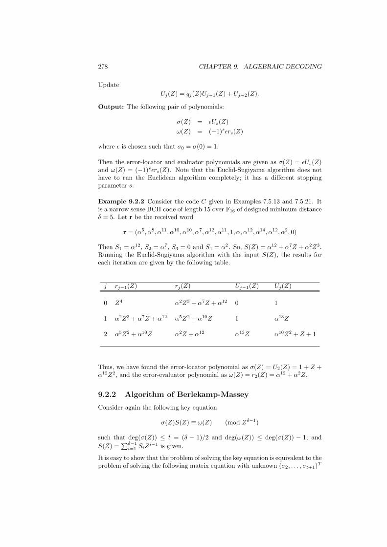
278 CHAPTER 9. ALGEBRAIC DECODING
Update
Uj(Z) = qj(Z)Uj−1(Z) + Uj−2(Z).
Output: The following pair of polynomials:
σ(Z) = εUs(Z)
ω(Z) = (−1)sεrs(Z)
where ε is chosen such that σ0 = σ(0) = 1.
Then the error-locator and evaluator polynomials are given as σ(Z) = εUs(Z)and ω(Z) = (−1)sεrs(Z). Note that the Euclid-Sugiyama algorithm does nothave to run the Euclidean algorithm completely; it has a different stoppingparameter s.
Example 9.2.2 Consider the code C given in Examples 7.5.13 and 7.5.21. Itis a narrow sense BCH code of length 15 over F16 of designed minimum distanceδ = 5. Let r be the received word
r = (α5, α8, α11, α10, α10, α7, α12, α11, 1, α, α12, α14, α12, α2, 0)
Then S1 = α12, S2 = α7, S3 = 0 and S4 = α2. So, S(Z) = α12 + α7Z + α2Z3.Running the Euclid-Sugiyama algorithm with the input S(Z), the results foreach iteration are given by the following table.
j rj−1(Z) rj(Z) Uj−1(Z) Uj(Z)
0 Z4 α2Z3 + α7Z + α12 0 1
1 α2Z3 + α7Z + α12 α5Z2 + α10Z 1 α13Z
2 α5Z2 + α10Z α2Z + α12 α13Z α10Z2 + Z + 1
Thus, we have found the error-locator polynomial as σ(Z) = U2(Z) = 1 + Z +α12Z2, and the error-evaluator polynomial as ω(Z) = r2(Z) = α12 + α2Z.
9.2.2 Algorithm of Berlekamp-Massey
Consider again the following key equation
σ(Z)S(Z) ≡ ω(Z) (mod Zδ−1)
such that deg(σ(Z)) ≤ t = (δ − 1)/2 and deg(ω(Z)) ≤ deg(σ(Z)) − 1; and
S(Z) =∑δ−1i=1 SiZ
i−1 is given.
It is easy to show that the problem of solving the key equation is equivalent to theproblem of solving the following matrix equation with unknown (σ2, . . . , σt+1)T
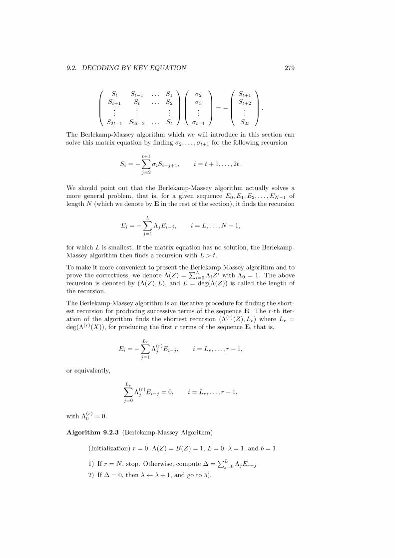
9.2. DECODING BY KEY EQUATION 279
St St−1 . . . S1
St+1 St . . . S2
......
...S2t−1 S2t−2 . . . St
σ2
σ3
...σt+1
= −
St+1
St+2
...S2t
.
The Berlekamp-Massey algorithm which we will introduce in this section cansolve this matrix equation by finding σ2, . . . , σt+1 for the following recursion
Si = −t+1∑j=2
σiSi−j+1, i = t+ 1, . . . , 2t.
We should point out that the Berlekamp-Massey algorithm actually solves amore general problem, that is, for a given sequence E0, E1, E2, . . . , EN−1 oflength N (which we denote by E in the rest of the section), it finds the recursion
Ei = −L∑j=1
ΛjEi−j , i = L, . . . , N − 1,
for which L is smallest. If the matrix equation has no solution, the Berlekamp-Massey algorithm then finds a recursion with L > t.
To make it more convenient to present the Berlekamp-Massey algorithm and toprove the correctness, we denote Λ(Z) =
∑Li=0 ΛiZ
i with Λ0 = 1. The aboverecursion is denoted by (Λ(Z), L), and L = deg(Λ(Z)) is called the length ofthe recursion.
The Berlekamp-Massey algorithm is an iterative procedure for finding the short-est recursion for producing successive terms of the sequence E. The r-th iter-ation of the algorithm finds the shortest recursion (Λ(r)(Z), Lr) where Lr =deg(Λ(r)(X)), for producing the first r terms of the sequence E, that is,
Ei = −Lr∑j=1
Λ(r)j Ei−j , i = Lr, . . . , r − 1,
or equivalently,
Lr∑j=0
Λ(r)j Ei−j = 0, i = Lr, . . . , r − 1,
with Λ(r)0 = 0.
Algorithm 9.2.3 (Berlekamp-Massey Algorithm)
(Initialization) r = 0, Λ(Z) = B(Z) = 1, L = 0, λ = 1, and b = 1.
1) If r = N , stop. Otherwise, compute ∆ =∑Lj=0 ΛjEr−j
2) If ∆ = 0, then λ← λ+ 1, and go to 5).
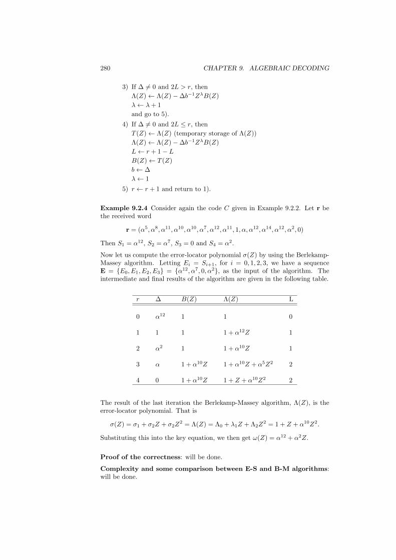
280 CHAPTER 9. ALGEBRAIC DECODING
3) If ∆ 6= 0 and 2L > r, then
Λ(Z)← Λ(Z)−∆b−1ZλB(Z)
λ← λ+ 1
and go to 5).
4) If ∆ 6= 0 and 2L ≤ r, then
T (Z)← Λ(Z) (temporary storage of Λ(Z))
Λ(Z)← Λ(Z)−∆b−1ZλB(Z)
L← r + 1− LB(Z)← T (Z)
b← ∆
λ← 1
5) r ← r + 1 and return to 1).
Example 9.2.4 Consider again the code C given in Example 9.2.2. Let r bethe received word
r = (α5, α8, α11, α10, α10, α7, α12, α11, 1, α, α12, α14, α12, α2, 0)
Then S1 = α12, S2 = α7, S3 = 0 and S4 = α2.
Now let us compute the error-locator polynomial σ(Z) by using the Berlekamp-Massey algorithm. Letting Ei = Si+1, for i = 0, 1, 2, 3, we have a sequenceE = E0, E1, E2, E3 = α12, α7, 0, α2, as the input of the algorithm. Theintermediate and final results of the algorithm are given in the following table.
r ∆ B(Z) Λ(Z) L
0 α12 1 1 0
1 1 1 1 + α12Z 1
2 α2 1 1 + α10Z 1
3 α 1 + α10Z 1 + α10Z + α5Z2 2
4 0 1 + α10Z 1 + Z + α10Z2 2
The result of the last iteration the Berlekamp-Massey algorithm, Λ(Z), is theerror-locator polynomial. That is
σ(Z) = σ1 + σ2Z + σ2Z2 = Λ(Z) = Λ0 + λ1Z + Λ2Z
2 = 1 + Z + α10Z2.
Substituting this into the key equation, we then get ω(Z) = α12 + α2Z.
Proof of the correctness: will be done.
Complexity and some comparison between E-S and B-M algorithms:will be done.
9.3. LIST DECODING BY SUDAN’S ALGORITHM 281
9.2.3 Exercises
9.2.1 Take α ∈ F∗16 with α4 = 1 + α as primitive element. Let C be the BCHcode over F16, of length 15 and designed minimum distance 5, with defining set1, 2, 3, 4, 6, 8, 9, 12. The generator polynomial is 1 +X4 +X6 +X7 +X8 (seeExample 7.3.13). Let
r = (0, 1, 0, 1, 1, 0, 0, 1, 0, 0, 0, 0, 0, 1, 0)
be a received word with respect to the code C. Find the syndrome polynomialS(Z). Write the key equation.
9.2.2 Consider the same code and same received word given in last exercise.Using the Berlekamp-Massey algorithm, compute the error-locator polynomial.Determine the number of errors occurred in the received word.
9.2.3 For the same code and same received word given the previous exer-cises, using the Euclid-Sugiyama algorithm, compute the error-locator and error-evaluator polynomials. Find the codeword which is closest to the received word.
9.2.4 Let α ∈ F∗16 with α4 = 1 + α as in Exercise 9.2.1. For the followingsequence E over F16, using the Berlekamp-Massey algorithm, find the shortestrecursion for producing successive terms of E:
E = α12, 1, α14, α13, 1, α11.
9.2.5 Consider the [15, 9, 7] Reed-Solomon code over F16 with defining set1, 2, 3, 4, 5, 6. Suppose the received word is
r = (0, 0, α11, 0, 0, α5, 0, α, 0, 0, 0, 0, 0, 0, 0).
Using the Berlekamp-Massey algorithm, find the codeword which is closest tothe received word.
9.3 List decoding by Sudan’s algorithm
A decoding algorithm is efficient if the complexity is bounded above by a poly-nomial in the code length. Brute-force decoding is not efficient, because for areceived word, it may need to compare qk codewords to return the most ap-propriate codeword. The idea behind list decoding is that instead of returninga unique codeword, the list decoder returns a small list of codewords. A list-decoding algorithm is efficient, if both the complexity and the size of the outputlist of the algorithm are bounded above by polynomials in the code length. Listdecoding was first introduced by Elias and Wozencraft in 1950’s.
We now describe a list decoder more precisely. Suppose C is a q-ary [n, k, d] code,t ≤ n is a positive integer. For any received word r = (r1, · · · , rn) ∈ Fnq , we referto any codeword c in C satisfying d(c, r) ≤ t as a t-consistent codeword. Let l bea positive integer less than or equal to qk. The code C is called (t, l)-decodable,if for any word r ∈ Fnq the number of t-consistent codewords is at most l. If forany received word, a list decoder can find all the t-consistent codewords, andthe output list has at most l codewords, then the decoder is called a (t, l)-listdecoder. In 1997 for the first time, Sudan proposed an efficient list-decodingalgorithm for Reed-Solomon codes. Later, Sudan’s list-decoding algorithm wasgeneralized to decoding algebraic-geometric codes and Reed-Muller codes.
282 CHAPTER 9. ALGEBRAIC DECODING
9.3.1 Error-correcting capacity
Suppose a decoding algorithm can find all the t-consistent codewords for anyreceived word. We call t the error-correcting capacity or decoding radius of thedecoding algorithm. As we have known in Section ??, for any [n, k, d] code, ift ≤
⌊d−1
2
⌋, then there is only one t-consistent codeword for any received word. In
other words, any [n, k, d] code is(⌊d−1
2
⌋, 1)-decodable. The decoding algorithms
in the previous sections return a unique codeword for any received word; andthey achieve an error-correcting capability less than or equal to
⌊d−1
2
⌋. The
list decoding achieves a decoding radius greater than⌊d−1
2
⌋; and the size of the
output list must be bounded above by a polynomial in n.
It is natural to ask the following question: For a [n, k, d] linear code C overFq, what is the maximal value t, such that C is (t, l)-decodable for a l which isbounded above by a polynomial in n? In the following, we give a lower boundon the maximum t such that C is (t, l)-decodable, which is called Johnson boundin the literature.
Proposition 9.3.1 Let C ⊆ Fnq be any linear code of minimum distance d =(1− 1/q)(1− β)n for 0 < β < 1. Let t = (1− 1/q)(1− γ)n for 0 < γ < 1. Thenfor any word r ∈ Fnq ,
|Bt(r) ∩ C| ≤
minn(q − 1), (1− β)/(γ2 − β)
, when γ >
√β
2n(q − 1)− 1, when γ =√β
where, Bt(r) = x ∈ Fnq | d(x, r) ≤ t is the Hamming ball of radius t around r.
We will prove this proposition later. We are now ready to state the Johnsonbound.
Theorem 9.3.2 For any linear code C ⊆ Fnq of relative minimum distanceδ = d/n, it is (t, l(n))-decodable with l(n) bounded above by a linear function inn, provided that
t
n≤(
1− 1
q
)(1−
√1− q
q − 1δ
).
Proof. For any received word r ∈ Fnq , the set of t-consistent codewordsc ∈ C | d(c, r) ≤ t = Bt(r) ∩ C.
Let β be a positive real number and β < 1. Denote d = (1− 1/q) (1− β)n. Lett = (1− 1/q) (1− γ)n for some 0 < γ < 1. Suppose
t
n≤(
1− 1
q
)(1−
√1− q
q − 1δ
).
Then, γ ≥√
1− qq−1 ·
dn =√β. By Proposition 9.3.1, the number of t-consistent
codewords, l(n), which is |Bt(r) ∩ C|, is bounded above by a polynomial in n,here q is viewed as a constant.
Remark 9.3.3 The classical error-correcting capability is t =⌊d−1
2
⌋. For a
linear [n, k] code of minimum distance d, we have d ≤ n− k + 1 (Note that forReed-Solomon codes, d = n− k + 1). Thus, the normalized capability
τ =t
n≤ 1
n·⌊n− k
2
⌋≈ 1
2− 1
2κ
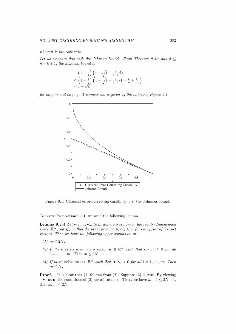
9.3. LIST DECODING BY SUDAN’S ALGORITHM 283
where κ is the code rate.
Let us compare this with the Johnson bound. From Theorem 9.3.2 and d ≤n− k + 1, the Johnson bound is(
1− 1q
)(1−
√1− q
q−1δ)
≤(
1− 1q
)(1−
√1− q
q−1 (1− kn + 1
n ))
≈ 1−√κ
for large n and large q. A comparison is given by the following Figure 9.1.
Figure 9.1: Classical error-correcting capability v.s. the Johnson bound.
To prove Proposition 9.3.1, we need the following lemma.
Lemma 9.3.4 Let v1, . . . ,vm be m non-zero vectors in the real N -dimensionalspace, RN , satisfying that the inner product, vi ·vj ≤ 0, for every pair of distinctvectors. Then we have the following upper bounds on m:
(1) m ≤ 2N .
(2) If there exists a non-zero vector u ∈ RN such that u · vi ≥ 0 for alli = 1, . . . ,m. Then m ≤ 2N − 1.
(3) If there exists an u ∈ RN such that u · vi > 0 for all i = 1, . . . ,m. Thenm ≤ N .
Proof. It is clear that (1) follows from (2). Suppose (2) is true. By viewing−v1 as u, the conditions of (2) are all satisfied. Thus, we have m− 1 ≤ 2N − 1,that is, m ≤ 2N .
284 CHAPTER 9. ALGEBRAIC DECODING
To prove (2), we will use induction on N . When N = 1, it is obvious thatm ≤ 2N −1 = 1. Otherwise, by the conditions, there are non-zero real numbersu, v1 and v2 such that u·v1 > 0 and u·v2 > 0, but v1 ·v2 < 0. This is impossible.Now considering N > 1, we can assume that m ≥ N + 1 (because if m ≤ N ,the result m ≤ 2N − 1 already holds). As the vectors v1, . . . ,vm are all in RN ,they must be linearly dependant. Let S ⊆ 1, 2, . . . ,m be a non-empty set ofminimum size for which there is a relation
∑i∈S aiv1 = 0 with all ai 6= 0. We
claim that the ais must all be positive or all be negative. In fact, if not, wecollect the terms with positive ais on one side and the terms with negative aison the other. We then get an equation
∑i∈S+ aivi =
∑j∈S− bjvj (which we
denote by w) with ai and bj all are positive, where S+ and S− are disjoint non-empty sets and S+ ∪ S− = S. By the minimality of S, w 6= 0. Thus, the innerproduct w ·w 6= 0. On the other hand, w ·w = (
∑i∈S+ aivi) · (
∑j∈S− bjvj) =∑
i,j(aibj)(vi · vj) ≤ 0 since aibj > 0 and vi · vj ≤ 0. This contradiction showsthat ais must all be positive or all be negative. Following this, we actually canassume that ai > 0 for all i ∈ S (otherwise, we can take a′i = −ai for a relation∑i∈S a
′iv1 = 0).
Without loss of generality, we assume that S = 1, 2, . . . , s. By the lineardependance
∑si=1 aivi = 0 with each ai > 0 and minimality of S, the vectors
v1, . . . ,vs must span a subspace V of RN of dimension s − 1. Now, for l =s + 1, . . . ,m, we have
∑si=1 aivi · vl = 0, as
∑si=1 aivi = 0. Since ai > 0 for
1 ≤ i ≤ s and all vi · vl ≤ 0, we have that vi is orthogonal to vl for all i, l with1 ≤ i ≤ s and s < l ≤ m. Similarly, we can prove that u is orthogonal to vifor i = 1, . . . , s. Therefore, the vectors vs+1, . . . ,vm and u are all in the dualspace V ⊥ which has dimension (N − s + 1). As s > 1, applying the inductionhypothesis to these vectors, we have m− s ≤ 2(N − s+ 1)− 1. Thus, we havem ≤ 2N − s+ 1 ≤ 2N − 1.
Now we prove (3). Suppose the result is not true, that is, m ≥ N + 1. Asabove, v1, . . . ,vm must be linearly dependant RN . Let S ⊆ 1, 2, . . . ,m bea non-empty set of minimum size for which there is a relation
∑i∈S aiv1 = 0
with all ai 6= 0. Again, we can assume that ai > 0 for all ai ∈ S. From this, wehave
∑si=1 aiu · vi = 0. But this is impossible since for each i we have ai > 0
and u · vi > 0. This contradiction shows m ≤ N .
Now we are ready to prove Proposition 9.3.1.
Proof of Proposition 9.3.1. We identify vectors in Fnq with vectors in Rqn inthe following way: First, we set an ordering for the elements of Fq, and denotethe elements as α1, α2, . . . , αq. Denote by ord(β) the order of element β ∈ Fqunder this ordering. For example, ord(β) = i, if β = αi Then, each element αi(1 ≤ i ≤ q) corresponds to the real unit vector of length q with a 1 in positioni and 0 elsewhere.
Without loss of generality, we assume that r = (αq, αq, . . . , αq). Denote byc1, c2, . . . , cm all the codewords of C that are in the Hamming ball Bt(r) wheret = (1− 1/q)(1− γ)n for some 0 < γ < 1.
We view each vector in Rqn as having n blocks each having q components,where the n blocks correspond to the n positions of the vectors in Fnq . Foreach l = 1, . . . , q, denote by el the unit vector of length q with 1 in the lthposition and 0 elsewhere. For i = 1, . . . ,m, the vector in Rqn associated with
9.3. LIST DECODING BY SUDAN’S ALGORITHM 285
the codeword ci, which we denote by di, has in its jth block the componentsof the vector eord(ci[j]), where ci[j] is the jth component of ci. The vector inRqn associated with the word r ∈ Fnq , which we denote by s, is defined similarly.
Let 1 ∈ Rqn be the all 1’s vector. We define v = λs + (1−λ)q 1 for 0 ≤ λ ≤ 1
that will be specified later. We observe that di and v are all in the space
defined by the intersection of the hyperplanes P ′j = x ∈ Rqn |q∑l=1
xj,l = 1
for j = 1, . . . , n. This fact implies that the vectors (di − v), for i = 1, . . . ,m,
are all in P =⋂nj=1 Pj where Pj = x ∈ Rqn |
q∑l=1
xj,l = 0. As P is an
n(q − 1)-dimensional subspace of Rqn, we have that the vectors (d1 − v), fori = 1, . . . ,m, are all in an n(q − 1)-dimensional space.
We will set the parameter λ so that the n(q − 1)-dimensional vectors (di − v),i = 1, . . . ,m, have all pairwise inner products less than 0. For i = 1, . . . ,m, letti = d(ci, r). Then ti ≤ t for every i, and
di · v = λ(di · s) + (1−λ)q (di · 1)
= λ(n− ti) + (1− λ)nq ≥ λ(n− t) + (1− λ)nq ,(9.1)
v · v = λ2n+ 2(1− λ)λn
q+ (1− λ)2n
q=n
q+ λ2(1− 1
q)n, (9.2)
di · dj = n− d(ci, cj) ≤ n− d, (9.3)
which implies that for i 6= j,
(di − v) · (dj − v) ≤ 2λt− d+ (1− 1
q)(1− λ)2n. (9.4)
Substituting t = (1 − 1/q)(1 − γ)n and d = (1 − 1/q)(1 − β)n into the aboveinequation, we have
(di − v) · (dj − v) ≤ (1− 1
q)n(β + λ2 − 2λγ). (9.5)
Thus, if γ > 12 (βλ + λ), we will have all pairwise inner products to be negative.
We pick λ to minimize (βλ +λ) by setting λ =√β. Now when γ >
√β, we have
(di − v) · (dj − v) < 0 for i 6= j.
9.3.2 Sudan’s algorithm
The algorithm of Sudan is applicable to Reed-Solomon codes, Reed-Mullercodes, algebraic-geometric codes, and some other families of codes. In thissub-section, we give a general description of the algorithm of Sudan.
Consider the following linear code
C = (f(P1), f(P2), · · · , f(Pn)) | f ∈ Fq[X1, . . . , Xm] and deg(f) < k ,
where Pi = (xi1, . . . , xim) ∈ Fmq for i = 1, . . . , n, and n ≤ qm. Note that whenm = 1, the code is a Reed-Solomon code or an extended Reed-Solomon code;when m ≥ 2, it is a Reed-Muller code.
286 CHAPTER 9. ALGEBRAIC DECODING
In the following algorithm and discussions, to simplify the statement we denote(i1, . . . , im) by i, Xi1
1 · · ·Ximm by X i, H(X1 +x1, . . . , Xm+xm, Y +y) by H(X+
x, Y + y),(j1i1
)· · ·(jmim
)by(ji
), and so on.
Algorithm 9.3.5 (The Algorithm of Sudan for List Decoding)
INPUT: The following parameters and a received word:
• Code length n and the integer k;
• n points in Fmq , namely, Pi := (xi1, . . . , xim) ∈ Fmq , i = 1, . . . , n;
• Received word r = (y1, . . . , yn) ∈ Fnq ;• Desired error-correcting radius t.
Step 0: Compute parameters r, s satisfying certain conditions that
we will give for specific families of codes in the following
sub-sections.
Step 1: Find a nonzero polynomial H(X,Y ) = H(X1, . . . , Xm, Y ) such
that
• The (1, . . . , 1, k−1)-weighted degree of H(X1, . . . , Xm, Y ) is at
most s;
• For i = 1, . . . , n, each point, (xi, yi) = (xi1, . . . , xim, yi) ∈ Fm+1q ,
is a zero of H(X,Y ) of multiplicity r.
Step 2: Find all the Y -roots of H(X,Y ) of degree less than k,namely, f = f(X1, . . . , Xm) of deg(f) < k such that H(X, f) is a
zero polynomial. For each such root, check if f(Pi) = yi for at
least n− t values of i ∈ 1, . . . , n. If so, include f in the
output list.
As we will see later, for an appropriately selected parameter t, the algorithm ofSudan can return a list containing all the t-consistent codewords in polynomialtime, with the size of the output list bounded above by a polynomial in codelength. So far, the best known record of error-correcting radius of list decodingby Sudan’s algorithm is the Johnson bound. In order to achieve this bound,prior to the actual decoding procedure, that is, Steps 1 and 2 of the algorithmabove, a pair of integers, r and s, should be carefully chosen, which will beused to find an appropriate polynomial H(X,Y ). The parameters r and s areindependent on received words. They are used for the decoding procedure forany received word, as long as they are determined. The actual decoding proce-dure consists two steps: Interpolation and Root Finding. By the interpolationprocedure, a nonzero polynomial H(X,Y ) is found. This polynomial containsall the polynomials which define the t-consistent codewords as its Y -roots. AY -root of H(X,Y ) is a polynomial f(X) satisfying that H(X, f(X)) is a zeropolynomial. The root-finding procedure finds and returns all these Y -roots;thus all the t-consistent codewords are found.
We now explain the terms: weighted degree and multiplicity of a zero of a poly-nomial, which we have used in the algorithm. Given integers a1, a2, . . . , al, the
9.3. LIST DECODING BY SUDAN’S ALGORITHM 287
(a1, a2, . . . , al)-weighted degree of a monomial αXd11 Xd2
2 · · ·Xdll (where α is the
coefficient of the monomial), is a1d1 + a2d2 + . . . + aldl. The (a1, a2, . . . , al)-weighted degree of a polynomial P (X1, X2, . . . , Xl) is the maximal (a1, a2, . . . , al)-weighted degree of its terms.
For a polynomial P (X) = α0 + α1X + α2X2 + . . . αdX
d, it is clear that 0 isa zero of P (X), i.e., P (0) = 0, if and only if α0 = 0. We say 0 is a zeroof multiplicity r of P (X), provided that α0 = α1 = . . . = αr−1 = 0 andαr 6= 0. For a nonzero value β, it is a zero of multiplicity r of P (X), providedthat 0 is a zero of multiplicity r of P (X + β). Similarly, for a multivariatepolynomial P (X1, X2, . . . , Xl) =
∑αi1,i2,...,ilX
i11 X
i22 · · ·X
ill , (0, 0, . . . , 0) is a
zero of multiplicity r of this polynomial, if and only if for all (i1, i2, . . . , il) withi1 + i2 + . . .+ il ≤ r − 1,
αi1,i2,...,il = 0
and there exists (i1, i2, . . . , il) with i1 + i2 + . . .+ il = r such that αi1,i2,...,il 6= 0.A point (β1, β2, . . . , βl) is a zero of multiplicity r of P (X1, X2, . . . , Xl), providedthat (0, 0, . . . , 0) is a zero of multiplicity r of P (X1 + β1, X2 + β2, . . . , Xl + βl).
Now we consider a polynomial that the Step 1 of Algorithm 9.3.5 seeks. SupposeH(X,Y ) =
∑αi,im+1
X iY im+1 is nonzero polynomial in X1, . . . , Xm, Y . It iseasy to prove that (we leave the proof to the reader as an exercise), for xi =(xi1, . . . , xim) and yi,
H(X + xi, Y + yi) =∑
j,jm+1
βj,jm+1XjY jm+1
where
βj,jm+1=∑j′1≥j1
· · ·∑
j′m≥jm
∑j′m+1≥jm+1
(j′
j
)(j′m+1
jm+1
)αj′,j′m+1
xj′−ji y
j′m+1−jm+1
i .
Step 1 of the algorithm seeks a nonzero polynomial H(X,Y ) such that its(1, . . . , 1, k − 1)-weighted degree is at most s, and for i = 1, . . . , n, each (x, yi)is a zero of H(X,Y ) of multiplicity r. Based on the discussion above, thiscan be done by solving a system consisting of the following homogeneous linearequations in unknowns αi,im+1 (which are coefficients of H(X,Y )),
∑j′1≥j1
· · ·∑
j′m≥jm
∑j′m+1≥jm+1
(j′
j
)(j′m+1
jm+1
)αj′,j′m+1
xj′−ji y
j′m+1−jm+1
i = 0.
for all i = 1, . . . , n, and for every j1, . . . , jm, jm+1 ≥ 0 with j1+· · ·+jm+jm+1 ≤r − 1; and
αi,im+1 = 0,
for every i1, . . . , im, im+1 ≥ 0 with i1 + · · ·+ im + (k − 1)im+1 ≥ s+ 1.
9.3.3 List decoding of Reed-Solomon codes
A Reed-Solomon code can be defined as a cyclic code generated by a generatorpolynomial (see Definition 8.1.1) or as an evaluation code (see Proposition 8.1.4).For the purpose of list decoding by Sudan’s algorithm, we view Reed-Solomon

288 CHAPTER 9. ALGEBRAIC DECODING
codes as evaluation codes. Note that since any non-zero element α ∈ Fq satisfiesαn = α, we have ev(Xnf(X)) = ev(f(X)) for any f(X) ∈ Fq[X], where n =q − 1. Therefore,
RSk(n, 1) = f(x1), f(x2), . . . , f(xn) | f(X) ∈ Fq[X],deg(f) < k
where x1, . . . , xn are n distinct nonzero elements of Fq.
In this subsection, we consider the list decoding of Reed-Solomon codesRSk(n, 1)and extended Reed-Solomon codes ERSk(n, 1), that is, the case m = 1 of thegeneral algorithm, Algorithm 9.3.5. As we will discuss later, Sudan’s algorithmcan be adapted to list decoding generalized Reed-Solomon codes (see Definition8.1.10).
The correctness and error-correcting capability of list-decoding algorithm aredependent on the parameters r and s. In the following, we first prove thecorrectness of the algorithm for appropriate choice of r and s. Then we calculatethe error-correcting capability.
We can prove the correctness of the list-decoding algorithm by proving: (1)There exists a nonzero polynomial H(X,Y ) satisfying the conditions given inStep 1 of Algorithm 9.3.5; and (2) All the polynomials f(X) satisfying theconditions in Step 2 are the Y -roots of H(X,Y ), that is, Y − f(X) dividesH(X,Y ).
Proposition 9.3.6 Consider a pair of parameters r and s.
(1) If r and s satisfy
n
(r + 1
2
)<s(s+ 2)
2(k − 1).
Then, a nonzero polynomial H(X,Y ) sought in Algorithm 9.3.5 does exist.
(2) If r and s satisfy
r(n− t) > s.
Then, for any polynomial f(X) of degree at most k−1 such that f(xi) = yifor at least n − t values of i ∈ 1, 2, . . . , n, the polynomial H(X,Y ) isdivisible by Y − f(X).
Proof. We first prove (1). As discussed in the previous subsection, a nonzeropolynomial H(X,Y ) exists as long as we have a nonzero solution of a sys-tem of homogeneous linear equations in unknowns αi1,i2 , i.e., the coefficients ofH(X,Y ). A nonzero solution of the system exists, provided that the numberof equations is strictly less than the number of unknowns. From the preciseexpression of the system (see the end of last subsection), it is easy to calcu-late the number of equations, which is n
(r+1
2
). Next, we compute the number
of unknowns. This number is equal to the number of monomials Xi1Y i2 of
9.3. LIST DECODING BY SUDAN’S ALGORITHM 289
(1, k − 1)-weighted degree at most s, which is
b sk−1 c∑i2=0
s−i2(k−1)∑i1=0
1
=b sk−1 c∑i2=0
(s+ 1− i2(k − 1))
= (s+ 1)(b sk−1c+ 1
)− k−1
2 bs
k−1c(b sk−1c+ 1
)≥(b sk−1c+ 1
) (s2 + 1
)≥ s
k−1 ·s+2
2
where bxc stands for the maximal integer less than or equal to x. Thus, weproved (1).
We now prove (2). Suppose H(X, f(X)) is not zero polynomial. Denote h(X) =H(X, f(X)). Let I = i | 1 ≤ i ≤ n and f(xi) = yi. We have |I| ≥ n − t.For any i = 1, . . . , n, as (xi, yi) is a zero of H(X,Y ) of multiplicity r, we canexpress H(X,Y ) =
∑j1+j2≥r
γj1,j2(X − xi)j1(Y − yi)j2 . Now, for any i ∈ I, we
have f(X)− yi = (X −xi)f1(X) for some f1(X), because f(xi)− yi = 0. Thus,we have
h(X) =∑
j1+j2≥r
γj1,j2(X−xi)j1(f(X)−yi)j2 =∑
j1+j2≥r
γj1,j2(X−xi)j1+j2(f1(X))j2 .
This implies that (X −xi)r divides h(X). Therefore, h(X) has a factor g(X) =∏i∈I(X − xi)r, which is a polynomial of degree at least r(n− t). On the other
hand, since H(X,Y ) has (1, k − 1)-weighted degree at most s and the degreeof f(X) is at most k − 1, the degree of h(X) is at most s, which is less thanr(n − t). This is impossible. Therefore, H(X, f(X) is a zero polynomial, thatis, Y − f(X) divides H(X,Y ).
Proposition 9.3.7 If t satisfies (n − t)2 > n(k − 1), then there exist r and s
satisfying both n(r+1
2
)< s(s+2)
2(k−1) and r(n− t) > s.
Proof. Set s = r(n− t)− 1. It suffices to prove that there exists r satisfying
n
(r + 1
2
)<
(r(n− t)− 1)(r(n− t) + 1)
2(k − 1)
which is equivalent to the following inequivalent
((n− t)2 − n(k − 1)) · r2 − n(k − 1) · r − 1 > 0.
Since (n− t)2 − n(k − 1) > 0, any integer r satisfying
r >n(k − 1) +
√n2(k − 1)2 + 4(n− t)2 − 4n(k − 1)
2(n− t)2 − 2n(k − 1)
satisfies the inequivalent above. Therefore, for the list-decoding algorithm to becorrect it suffices by setting the integers r and s as
r =
⌊n(k − 1) +
√n2(k − 1)2 + 4(n− t)2 − 4n(k − 1)
2(n− t)2 − 2n(k − 1)
⌋+ 1
290 CHAPTER 9. ALGEBRAIC DECODING
and s = r(n− t)− 1.
We give the following result, Theorem 9.3.8, which is a straightforward corollaryof the two propositions.
Theorem 9.3.8 For a [n, k] Reed-Solomon or extended Reed-Solomon code thelist-decoding algorithm, Algorithm 9.3.5, can correctly find all the codewords cwithin distance t from the received word r, i.e., d(r, c) ≤ t, provided
t < n−√n(k − 1).
Remark 9.3.9 Note that for a [n, k] Reed-Solomon code, the minimum distanced = n− k+ 1 which implies that k− 1 = n− d. Substituting this into the boundon error-correcting capability in the theorem above, we have
t
n< 1−
√1− d
n.
This shows that the list-decoding of Reed-Solomon codes achieves the Johnsonbound (see Theorem 9.3.2).
Regarding the size of the output list of the list-decoding algorithm, we have thefollowing theorem.
Theorem 9.3.10 Consider a [n, k] Reed-Solomon or extended Reed-Solomoncode. For any t < n−
√n(k − 1) and any received word, the number of t-consist
codewords is O(√n3k).
Proof. From Proposition 9.3.6, we actually have proved that the number N ofthe t-consist codewords is bounded from above by the degree degY (H(X,Y )).Since the (1, k − 1)-weighted degree of H(X,Y ) is at most s, we have N ≤degY (H(X,Y )) ≤ b s
(k−1)c. By the choices of r and s, s(k−1) = O
(n(k−1)(n−t)
k−1
)=
O(n(n− t)). Corresponding to the largest permissible value of t for the t-consistcodewords, we can choose n− t = b
√n(k − 1)c+ 1. Thus,
N = O(n(n− t)) = O(√n3(k − 1)) = O(
√n3k).
Let us analyze the complexity of the list decoding of a [n, k] Reed-Solomoncode. As we have seen, the decoding algorithm consists of two main steps.Step 1 is in fact reduced to a problem of solving a system of homogeneouslinear equations, which can be implemented making use of Gaussian elimination
with time complexity O((
s(s+2)2(k−1)
)3)
= O(n3) where s(s+2)2(k−1) is the number of
unknowns of the system of homogeneous linear equations, and s is given as inProposition 9.3.7.
The second step is a problem of finding Y -roots the polynomial H(X,Y ). Thiscan be implemented by using a fast root-finding algorithm proposed by Rothand Ruckenstein in time complexity O(nk).
9.3. LIST DECODING BY SUDAN’S ALGORITHM 291
9.3.4 List Decoding of Reed-Muller codes
We consider the list decoding of Reed-Muller codes in this subsection. Letn = qm and P1, . . . , Pn be an enumeration of the points of Fmq . Recall that theq-ary Reed-Muller code RMq(u,m) of order u in m variables is defined as
RMq(u,m) = (f(P1), . . . , f(Pn)) | f ∈ Fq[X1, . . . , Xm], deg(f) ≤ u.
Note that when m = 1, the code RMq(u, 1) is actually an extended Reed-Solomon code.
From Proposition 8.4.4, RMq(u,m) is a subfield subcode of RMqm(n − d, 1)where d be the minimum distance of RMq(u,m), that is
RMq(u,m) ⊆ RMqm(n− d, 1) ∩ Fnq .
Here RMqm(n − d, 1) is an extended Reed-Solomon code over Fqm of lengthn and dimension k = n − d + 1. We now give a list-decoding algorithm forRMq(u,m) as follows.
Algorithm 9.3.11 (List-Decoding Algorithm for Reed-Muller Codes)
INPUT: Code length n and a received word r = (y1, . . . , yn) ∈ Fnq .
Step 0: Do the following:
(1) Compute the minimum distance d of RMq(u,m) and a parameter
t = dn−√n(n− d)− 1e.
(2) Construct the extension field Fqm using an irreducible
polynomial of degree m over Fq.(3) Generate the code RMqm(n− d, 1).
(4) Construct a parity check matrix H over Fq for the code
RMq(u,m).
Step 1: Using the list-decoding algorithm for Reed-Solomon codes
over Fqm , find L(1), the set of all codewords c ∈ RMqm(n− d, 1)satisfying
d(c, r) ≤ t.
Step 2: For every c ∈ L(1), check if c ∈ Fnq , if so, append c to L(2).
Step 3: For every c ∈ L(2), check if HcT = 0, if so, append c to L.Output L.
From Theorems 9.3.8 and 9.3.10, we have the following theorem.
Theorem 9.3.12 Denote by d the minimum distance of the q-ary Reed-Mullercode RMq(u,m). Then RMq(u,m) is (t, l)-decodable, provided that
t < n−√n(n− d) and l = O(
√(n− d)n3).
The algorithm above correctly finds all the t-consistent codewords for any re-ceived vector r ∈ Fnq .
292 CHAPTER 9. ALGEBRAIC DECODING
Remark 9.3.13 Note that Algorithm 9.3.11 outputs a set of t-consistent code-words of the q-ary Reed-Muller code defined by the enumeration of points ofFmq , say P1, P2, . . . , Pn, specified in Section 7.4.2. If RMq(u,m) is definedby another enumeration of the points of Fmq , say P ′1, P
′2, . . . , P
′n, we can get
the correct t-consistent codewords by the following steps: (1) Find the permu-tation π such that Pi = P ′π(i), i = 1, 2, . . . , n, and the inverse permutation
π−1. (2) Let r∗ = (rπ(1), rπ(2), . . . , rπ(n)). Then, go to Steps 0-2 of Algo-rithm 9.3.11 with r∗. (3) For every codeword c = (c1, c2, . . . , cn) ∈ L, letπ−1(c) = (cπ−1(1), cπ−1(2), . . . , cπ−1(n)). Then, π−1(L) = π−1(c) | c ∈ L isthe set of t-consistent codewords of RMq(u,m).
Now, let us consider the complexity of Algorithm 9.3.11 In Step 0, to constructthe extension field Fqm , it is necessary to find an irreducible polynomial g(x)of degree m over Fq. It is well known that there are efficient algorithms forfinding irreducible polynomials over finite fields. For example, a probabilisticalgorithm proposed by V. Shoup in 1994 can find an irreducible polynomial ofdegree m over Fq with expected number of O((m2logm+mlogq)logmloglogm)field operations in Fq.
To generate the Reed-Solomon code GRSn−d+1(a,1) over Fqm , we need to finda primitive element of Fqm . With a procedure by I.E. Shparlinski in 1993, aprimitive element of Fqm can be found in deterministic time O((qm)1/4+ε) =O(n1/4+ε), where n = qm is the length of the code, ε denotes an arbitrarypositive number.
Step 1 of Algorithm 9.3.11 can be implemented using the list-decoding algo-rithm in for Reed-Solomon code GRSn−d+1(a,1) over Fqm . From the previoussubsection, it can be implemented to run in O(n3) field operations in Fqm .
So, the implementation of Algorithm 9.3.11 requires O(n) field operations in Fqand O(n3) field operations in Fqm .
9.3.5 Exercises
9.3.1 Let P (X1, . . . , Xl) =∑
i1,...,il
αi1,...,ilXi11 · · ·X
ill be a polynomial in vari-
ables X1, . . . , Xl with coefficients αi1,...,il in a field F. Prove that for any(a1, . . . , al) ∈ Fl,
P (X1 + a1, . . . , Xl + al) =∑
j1,...,jl
βj1,...,jlXj11 · · ·X
jll
where
βj1,...,jl =∑j′1≥j1
· · ·∑j′l≥jl
(j′1j1
)· · ·(j′ljl
)αj′1,...,j′la
j′1−j11 · · · aj
′l−jll .
9.4 Notes
Many cyclic codes have error-correcting pairs, for this we refer to Duursma andKotter [53, 54].
9.4. NOTES 293
The algorithms of Berlekamp-Massey [11, 79] and Sugiyama [118] both haveO(t2) as an estimation of the complexity, where t is the number of correctederrors. In fact the algorithms are equivalent as shown in [50, 65]. The applicationof a fast computation of the gcd of two polynomials in [4, Chap. 16, §8.9] incomputing a solution of the key equation gives as complexity O(t log2(t)) by[69, 104].

294 CHAPTER 9. ALGEBRAIC DECODING
Chapter 10
Cryptography
Stanislav Bulygin
This chapter is aiming at giving an overview of topics from cryptography. In par-ticular, we cover symmetric as well as asymmetric cryptography. When talkingabout symmetric cryptography, we concentrate on a notion of a block cipher,as a mean to implement symmetric cryptosystems in practical environments.Asymmetric cryptography is represented by the RSA and El Gamal cryptosys-tems, as well as code-based cryptosystems due to McEliece and Niederreiter. Wealso take a look at other aspects such as authentication codes, secret sharing,and linear feedback shift registers. The material of this chapter is quite ba-sic, but we elaborate more on several topics. Especially we should connectionsto codes and related structures where applicable. The basic idea of algebraicattacks on block ciphers is considered in the next chapter, Section 11.3.
10.1 Symmetric cryptography and block ciphers
10.1.1 Symmetric cryptography
This section is devoted to the Symmetric cryptosystems. The idea behind theseis quite simple and thus was basically known for quite along time. The task isto convey a secret between two parties, called traditionally Alice and Bob, sothat figuring the secret out is not possible without knowledge of some additionalinformation. This additional information is called a secret key and is supposed tobe known only to the two communicating parties. The secrecy of the transmittedmessage rests entirely upon the knowledge of this secret key, and thus if anadversary or an eavesdropper, traditionally called Eve, is able to find out thekey, then the whole secret communication is corrupted. Now let us take a lookat the formal definition.
Definition 10.1.1 The symmetric cryptosystem is defined by the followingdata:
• The plaintext space P and the ciphertext space C.
295
296 CHAPTER 10. CRYPTOGRAPHY
• Ee : P → C|e ∈ K and Dd : C → P|d ∈ K are the sets of encryptionand decryption transformations, which are bijections from P to C and fromC to P resp.
• The above transformations are parametrized by the key space K.
• Given an associated pair (e, d), so that a property ∀p ∈ P : Dd(Ee(p)) = pholds, knowing e it is ”computationally easy” to find out d and vise versa.
The pair (e, d) is called secret key . Moreover, e is called the encryption key andd is called the decryption key .
Note that often the counterparts e and d coincide. This gives a reason for thename ”symmetric”. There exist also cryptosystems in which knowledge of anencryption key e does not reveal (i.e. it is ”computationally hard” to find) anassociated decryption key d. So encryption keys can be made public, and suchcryptosystems are called asymmetric or public see Section 10.2.Of course, one should specify exactly what are P, C,K and the transformations.Let us take a look at a concrete example.
Example 10.1.2 The first use of a symmetric cryptosystem is conventionallyattributed to Julius Caesar. He used the following cryptosystem for communi-cation with his generals, which is historically called Caesar cipher . Let P and Cbe the sets of all strings composed of letters from the English (Latin for Caesar)alphabet A = A,B,C, . . . , Z. Let K = 0, 1, 2, . . . , 25. Now an encryptiontransformation Ee given a plaintext p = (p1, . . . , pn), pi ∈ A, i = 1, . . . , n doesthe following. For each i = 1, . . . , n one determines a position of pi in the al-phabet A (”A” being 0, ”B” being 1, . . . , ”Z” being 25). Next one finds aletter in A that stands e positions to the left, thus finding a letter ci; one needsto overlap if the beginning of A is reached. So with the enumeration of A asabove, we have ci = pi − e ( mod 26). In this way a ciphertext c = (c1, . . . , cn)is obtained. Decryption key is given by d = −e ( mod 26), or, equivalently, fordecryption one needs to shift letters e positions to the right.Julius Caesar used e = 3 for his cryptosystem. Let us consider an example. Forthe plaintext p =”BRUTUS IS AN ASSASSIN”, the ciphertext (if we ignorespaces during the encryption) looks like c =”YORQRP FP XK XOOXOOFK”.To decrypt one simply shifts back 3 positions to the right.
10.1.2 Block ciphers. Simple examples
The above is a simple example of a so-called substitution cipher , which is inturn an instance of a block cipher. Block ciphers, among other things, providea practical realization of symmetric cryptosystems. They can also be used forconstructing other cryptographic primitives, like pseudorandom number genera-tors, authentication codes (Section 10.3), hash functions. The formal definitionfollows.
Definition 10.1.3 The n-bit block cipher is defined as a mapping E : An×K →An, where A is an alphabet set and K is the key space and for each k ∈ K themapping E(·, k) =: Ek : 0, 1n → 0, 1n is invertible. Ek is the encryptiontransformation for the key k, and E−1
k = Dk is the decryption transformation.If Ek(p) = c, then c is the ciphertext of the plaintext p under the key k.
10.1. SYMMETRIC CRYPTOGRAPHY AND BLOCK CIPHERS 297
It is common to work with the binary alphabet, i.e. A = 0, 1. In such case,ideally we would like to have a block cipher that is random in the sense that itimplements all (2n)! bijections from 0, 1n to 0, 1n. In practice, though, itis quite expensive to have such a cipher. So when designing a block cipher wecare that it behaves like a random one, i.e. for a randomly chosen key k ∈ Kthe encryption transformation Ek should appear random. If one is able to finddistinctions of Ek, where k is in some subset Kweak, from the random transfor-mation, then it is an evidence of a weakness of the cipher. Such subset Kweakis called the subset of weak keys; we will turn back to this later when talkingabout DES.Now we present several simple examples of block ciphers. We consider permu-tation and substitution ciphers that were used quite intensively in the past (seeNotes) and some fundamental ideas thereof appear also in the modern ciphers.
Example 10.1.4 (Permutation or transposition cipher) The idea of this cipheris to partition the plaintext into blocks and perform a permutation of elementsin that block. More formally, partition the plaintext into blocks of the formp = p1 . . . pt and then permute: c = Ek(p) = pk(1), . . . , pk(t). A number t iscalled a period of the cipher. The key space K now is the set of all permuta-tions of 1, . . . , t : K = St. For example let the plaintext be p =”CODINGAND CRYPTO”, let t = 5, and k = (4, 2, 5, 3, 1). If we remove the spaces andpartition p into 3 blocks we obtain c =”INCODDCGANTORYP”. Used alonepermutation cipher does not provide good security (see below), but in combina-tion with other techniques it is used also in modern ciphers to provide diffusionin a ciphertext.
Example 10.1.5 We can use Sage system to run the previous example. Thecode looks as follows.> S = AlphabeticStrings()
> E = TranspositionCryptosystem(S,5)
> K = PermutationGroupElement(’(4,2,5,3,1)’)
> L = E.inverse_key(K)
> M = S("CODINGANDCRYPTO")
> e = E(K)
> c = E(L)
> e(M)
INCODDCGANTORYP
> c(e(M))
CODINGANDCRYPTO
One can also choose a random key for encryption:> KR = E.random_key()
> KR
(1,4,2,3)
> LR = E.inverse_key(KR)
> LR
(1,3,2,4)
> eR = E(KR)
> cR = E(LR)
> eR(M)
IDCONDNGACTPRYO
298 CHAPTER 10. CRYPTOGRAPHY
> cR(eR(M))
CODINGANDCRYPTO
Example 10.1.6 (Substitution cipher) An idea behind monoalphabetic substi-tution cipher is to provide substitution of every symbol in a plaintext by someother symbol from a chosen alphabet. Formally, let A be the alphabet, so thatplaintexts and ciphertexts are composed of symbols from A. For the plaintextp = p1 . . . pn the ciphertext c is obtained as c = Ek(p) = k(p1), . . . , k(pn). Thekey space now is the set of all permutations of A : K = S|A|. In Example10.1.2 we have already seen an instance of such a cipher. There k was chosento be k = (23, 24, 25, 0, 1, . . . , 21, 22). Again, used alone monoalphabetic cipheris insecure, but as a basic idea is used in modern ciphers to provide confusionin a ciphertext.There is also a polyalphabetic substitution cipher. Let the key k be defined as asequence of permutations on A : k = (k1, . . . , kt), where t is the period. Thenevery t symbols of the plaintext p are mapped to t symbols of the ciphertext cas c = k1(p1), . . . , kt(pt). Simplifying ki to shifting by li symbols to the rightwe obtain ci = pi+ li ( mod |A|). Such cipher is called simple Vigenere cipher .
Example 10.1.7 The Sage-code for a substitution cipher encryption is givenbelow.> S = AlphabeticStrings()
> E = SubstitutionCryptosystem(S)
> K = E.random_key()
> K
ZYNJQHLBSPEOCMDAXWVRUTIKGF
> L = E.inverse_key(K)
> M = S("CODINGANDCRYPTO")
> e = E(K)
> e(M)
NDJSMLZMJNWGARD
> c = E(L)
Here the string ZYNJQHLBSPEOCMDAXWVRUTIKGF shows the permutation of thealphabet. Namely, the letter A is mapped to Z, the letter B is mapped to Y etc.One can also provide the permutation explicitly as follows> K = S(’MHKENLQSCDFGBIAYOUTZXJVWPR’)
> e = E(K)
> e(M)
KAECIQMIEKUPYZA
A piece of code for working with the simple Vigenere cipher is provided below.> S = AlphabeticStrings()
> E = VigenereCryptosystem(S,15)
> K = S(’XSPUDFOQLRMRDJS’)
> L = E.inverse_key(K)
> M = S("CODINGANDCRYPTO")
> e = E(K)
> e(M)
ZGSCQLODOTDPSCG
> c = E(L)
> c(e(M))
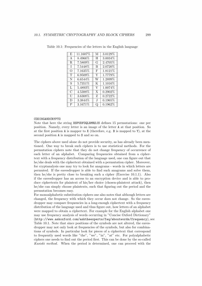
10.1. SYMMETRIC CRYPTOGRAPHY AND BLOCK CIPHERS 299
Table 10.1: Frequencies of the letters in the English language
E 11.1607% M 3.0129%A 8.4966% H 3.0034%R 7.5809% G 2.4705%I 7.5448% B 2.0720%O 7.1635% F 1.8121%T 6.9509% Y 1.7779%N 6.6544% W 1.2899%S 5.7351% K 1.1016%L 5.4893% V 1.0074%C 4.5388% X 0.2902%U 3.6308% Z 0.2722%D 3.3844% J 0.1965%P 3.1671% Q 0.1962%
CODINGANDCRYPTO
Note that here the string XSPUDFOQLRMRDJS defines 15 permutations: one perposition. Namely, every letter is an image of the letter A at that position. Soat the first position A is mapper to X (therefore, e.g. B is mapped to Y), at thesecond position A is mapped to S and so on.
The ciphers above used alone do not provide security, as has already been men-tioned. One way to break such ciphers is to use statistical methods. For thepermutation ciphers note that they do not change frequency of occurrence ofeach letter of an alphabet. Comparing frequencies obtained from a cipher-text with a frequency distribution of the language used, one can figure out thathe/she deals with the ciphertext obtained with a permutation cipher. Moreover,for cryptanalysis one may try to look for anagrams - words in which letters arepermuted. If the eavesdropper is able to find such anagrams and solve them,then he/she is pretty close to breaking such a cipher (Exercise 10.1.1). Alsoif the eavesdropper has an access to an encryption device and is able to pro-duce ciphertexts for plaintext of his/her choice (chosen-plaintext attack), thenhe/she can simply choose plaintexts, such that figuring out the period and thepermutation becomes easy.For monoalphabetic substitution ciphers one also notes that although letters arechanged, the frequency with which they occur does not change. So the eaves-dropper may compare frequencies in a long-enough ciphertext with a frequencydistribution of the language used and thus figure out, how letters of an alphabetwere mapped to obtain a ciphertext. For example for the English alphabet onemay use frequency analysis of words occurring in ”Concise Oxford Dictionary”(http://www.askoxford.com/asktheexperts/faq/aboutwords/frequency), seeTable 10.1. Note that since positions of the symbols are not altered, the eaves-dropper may not only look at frequencies of the symbols, but also for combina-tions of symbols. In particular look for pieces of a ciphertext that correspondto frequently used words like ”the”, ”we”, ”in”, ”at” etc. For polyalphabeticciphers one needs to find out the period first. This can be done by the so-calledKasiski method . When the period is determined, one can proceed with the
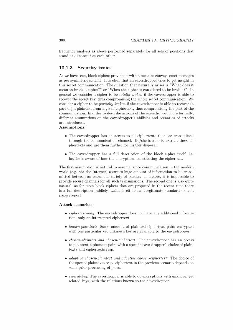
300 CHAPTER 10. CRYPTOGRAPHY
frequency analysis as above performed separately for all sets of positions thatstand at distance t at each other.
10.1.3 Security issues
As we have seen, block ciphers provide us with a mean to convey secret messagesas per symmetric scheme. It is clear that an eavesdropper tries to get insight inthis secret communication. The question that naturally arises is ”What does itmean to break a cipher?” or ”When the cipher is considered to be broken?”. Ingeneral we consider a cipher to be totally broken if the eavesdropper is able torecover the secret key, thus compromising the whole secret communication. Weconsider a cipher to be partially broken if the eavesdropper is able to recover (apart of) a plaintext from a given ciphertext, thus compromising the part of thecommunication. In order to describe actions of the eavesdropper more formally,different assumptions on the eavesdropper’s abilities and scenarios of attacksare introduced.Assumptions:
• The eavesdropper has an access to all ciphertexts that are transmittedthrough the communication channel. He/she is able to extract these ci-phertexts and use them further for his/her disposal.
• The eavesdropper has a full description of the block cipher itself, i.e.he/she is aware of how the encryptions constituting the cipher act.
The first assumption is natural to assume, since communication in the modernworld (e.g. via the Internet) assumes huge amount of information to be trans-mitted between an enormous variety of parties. Therefore, it is impossible toprovide secure channels for all such transmissions. The second one is also quitenatural, as for most block ciphers that are proposed in the recent time thereis a full description publicly available either as a legitimate standard or as apaper/report.
Attack scenarios:
• ciphertext-only: The eavesdropper does not have any additional informa-tion, only an intercepted ciphertext.
• known-plaintext: Some amount of plaintext-ciphertext pairs encryptedwith one particular yet unknown key are available to the eavesdropper.
• chosen-plaintext and chosen-ciphertext: The eavesdropper has an accessto plaintext-ciphertext pairs with a specific eavesdropper’s choice of plain-texts and ciphertexts resp.
• adaptive chosen-plaintext and adaptive chosen-ciphertext: The choice ofthe special plaintexts resp. ciphertext in the previous scenario depends onsome prior processing of pairs.
• related-key: The eavesdropper is able to do encryptions with unknown yetrelated keys, with the relations known to the eavesdropper.
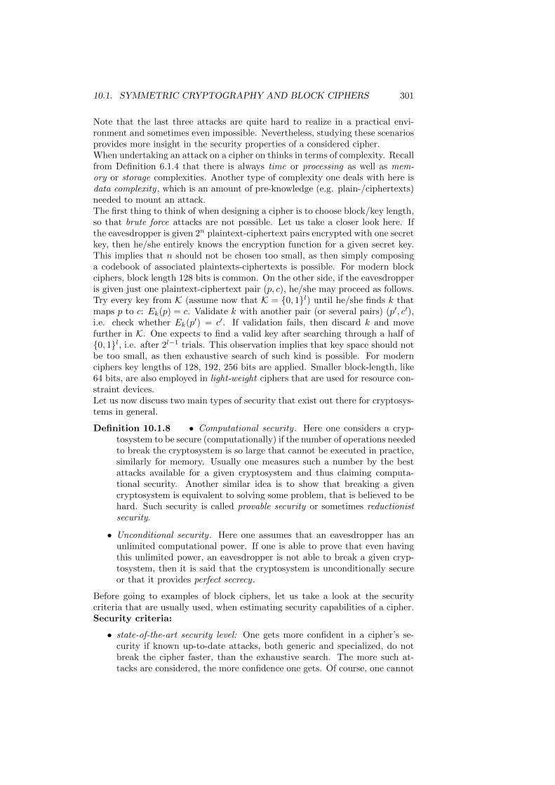
10.1. SYMMETRIC CRYPTOGRAPHY AND BLOCK CIPHERS 301
Note that the last three attacks are quite hard to realize in a practical envi-ronment and sometimes even impossible. Nevertheless, studying these scenariosprovides more insight in the security properties of a considered cipher.When undertaking an attack on a cipher on thinks in terms of complexity. Recallfrom Definition 6.1.4 that there is always time or processing as well as mem-ory or storage complexities. Another type of complexity one deals with here isdata complexity , which is an amount of pre-knowledge (e.g. plain-/ciphertexts)needed to mount an attack.The first thing to think of when designing a cipher is to choose block/key length,so that brute force attacks are not possible. Let us take a closer look here. Ifthe eavesdropper is given 2n plaintext-ciphertext pairs encrypted with one secretkey, then he/she entirely knows the encryption function for a given secret key.This implies that n should not be chosen too small, as then simply composinga codebook of associated plaintexts-ciphertexts is possible. For modern blockciphers, block length 128 bits is common. On the other side, if the eavesdropperis given just one plaintext-ciphertext pair (p, c), he/she may proceed as follows.Try every key from K (assume now that K = 0, 1l) until he/she finds k thatmaps p to c: Ek(p) = c. Validate k with another pair (or several pairs) (p′, c′),i.e. check whether Ek(p′) = c′. If validation fails, then discard k and movefurther in K. One expects to find a valid key after searching through a half of0, 1l, i.e. after 2l−1 trials. This observation implies that key space should notbe too small, as then exhaustive search of such kind is possible. For modernciphers key lengths of 128, 192, 256 bits are applied. Smaller block-length, like64 bits, are also employed in light-weight ciphers that are used for resource con-straint devices.Let us now discuss two main types of security that exist out there for cryptosys-tems in general.
Definition 10.1.8 • Computational security . Here one considers a cryp-tosystem to be secure (computationally) if the number of operations neededto break the cryptosystem is so large that cannot be executed in practice,similarly for memory. Usually one measures such a number by the bestattacks available for a given cryptosystem and thus claiming computa-tional security. Another similar idea is to show that breaking a givencryptosystem is equivalent to solving some problem, that is believed to behard. Such security is called provable security or sometimes reductionistsecurity.
• Unconditional security . Here one assumes that an eavesdropper has anunlimited computational power. If one is able to prove that even havingthis unlimited power, an eavesdropper is not able to break a given cryp-tosystem, then it is said that the cryptosystem is unconditionally secureor that it provides perfect secrecy .
Before going to examples of block ciphers, let us take a look at the securitycriteria that are usually used, when estimating security capabilities of a cipher.Security criteria:
• state-of-the-art security level: One gets more confident in a cipher’s se-curity if known up-to-date attacks, both generic and specialized, do notbreak the cipher faster, than the exhaustive search. The more such at-tacks are considered, the more confidence one gets. Of course, one cannot
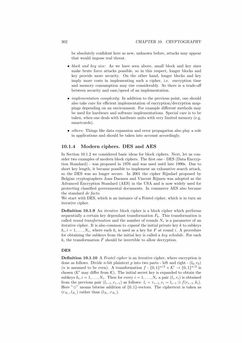
302 CHAPTER 10. CRYPTOGRAPHY
be absolutely confident here as new, unknown before, attacks may appearthat would impose real threat.
• block and key size: As we have seen above, small block and key sizesmake brute force attacks possible, so in this respect, longer blocks andkey provide more security. On the other hand, longer blocks and keyimply more costs in implementing such a cipher, i.e. encryption timeand memory consumption may rise considerably. So there is a trade-offbetween security and ease/speed of an implementation.
• implementation complexity: In addition to the previous point, one shouldalso take care for efficient implementation of encryption/decryption map-pings depending on an environment. For example different methods maybe used for hardware and software implementations. Special care is to betaken, when one deals with hardware units with very limited memory (e.g.smartcards).
• others: Things like data expansion and error propagation also play a rolein applications and should be taken into account accordingly.
10.1.4 Modern ciphers. DES and AES
In Section 10.1.2 we considered basic ideas for block ciphers. Next, let us con-sider two examples of modern block ciphers. The first one - DES (Data Encryp-tion Standard) - was proposed in 1976 and was used until late 1990s. Due toshort key length, it became possible to implement an exhaustive search attack,so the DES was no longer secure. In 2001 the cipher Rijndael proposed byBelgian cryptographers Joan Daemen and Vincent Rijmen was adopted as theAdvanced Encryption Standard (AES) in the USA and is now widely used forprotecting classified governmental documents. In commerce AES also becamethe standard de facto.We start with DES, which is an instance of a Feistel cipher, which is in turn aniterative cipher.
Definition 10.1.9 An iterative block cipher is a block cipher which performssequentially a certain key dependant transformation Fk. This transformation iscalled round transformation and the number of rounds Nr is a parameter of aniterative cipher. It is also common to expand the initial private key k to subkeyski, i = 1, . . . , Nr, where each ki is used as a key for F at round i. A procedurefor obtaining the subkeys from the initial key is called a key schedule. For eachki the transformation F should be invertible to allow decryption.
DES
Definition 10.1.10 A Feistel cipher is an iterative cipher, where encryption isdone as follows. Divide n-bit plaintext p into two parts - left and right - (l0, r0)(n is assumed to be even). A transformation f : 0, 1n/2 × K′ → 0, 1n/2 ischosen (K′ may differ from K). The initial secret key is expanded to obtain thesubkeys ki, i = 1, . . . , Nr. Then for every i = 1, . . . , Nr a pair (li, ri) is obtainedfrom the previous pair (li−1, ri−1) as follows: li = ri−1, ri = li−1 ⊕ f(ri−1, ki).Here ”⊕” means bitwise addition of 0, 1-vectors. The ciphertext is taken as(rNr , lNr ) rather than (lNr , rNr ).
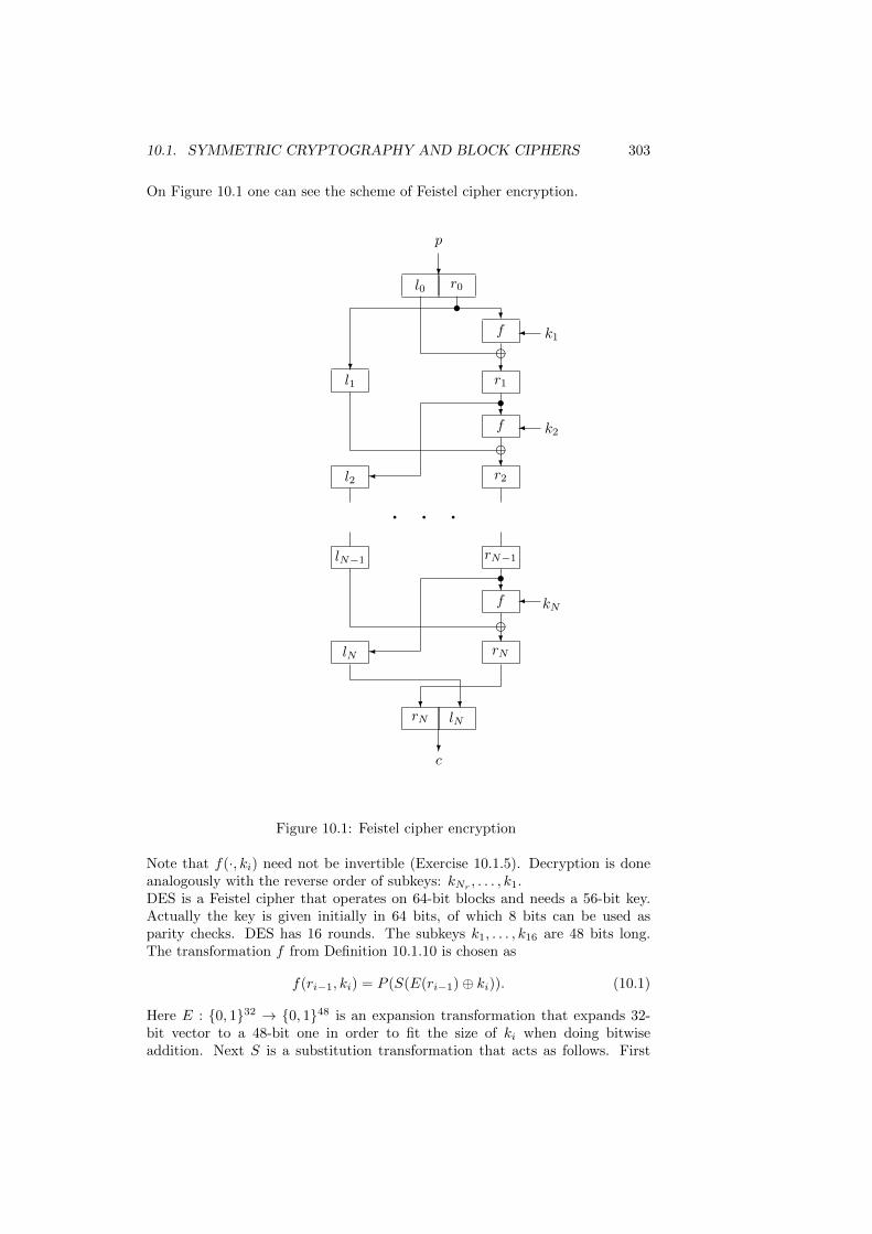
10.1. SYMMETRIC CRYPTOGRAPHY AND BLOCK CIPHERS 303
On Figure 10.1 one can see the scheme of Feistel cipher encryption.
p
?l0 r0s
?l1
e?f k1
?r1
?s
l2
ef k2
?r2
q q qrN−1
?f kN
?rN
slN
lN−1
e
??rN lN
?c
Figure 10.1: Feistel cipher encryption
Note that f(·, ki) need not be invertible (Exercise 10.1.5). Decryption is doneanalogously with the reverse order of subkeys: kNr
, . . . , k1.DES is a Feistel cipher that operates on 64-bit blocks and needs a 56-bit key.Actually the key is given initially in 64 bits, of which 8 bits can be used asparity checks. DES has 16 rounds. The subkeys k1, . . . , k16 are 48 bits long.The transformation f from Definition 10.1.10 is chosen as
f(ri−1, ki) = P (S(E(ri−1)⊕ ki)). (10.1)
Here E : 0, 132 → 0, 148 is an expansion transformation that expands 32-bit vector to a 48-bit one in order to fit the size of ki when doing bitwiseaddition. Next S is a substitution transformation that acts as follows. First
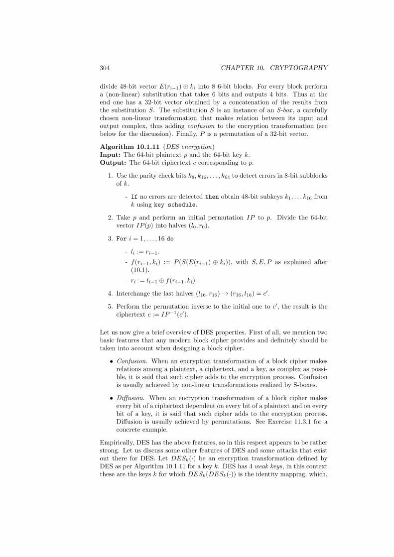
304 CHAPTER 10. CRYPTOGRAPHY
divide 48-bit vector E(ri−1) ⊕ ki into 8 6-bit blocks. For every block performa (non-linear) substitution that takes 6 bits and outputs 4 bits. Thus at theend one has a 32-bit vector obtained by a concatenation of the results fromthe substitution S. The substitution S is an instance of an S-box , a carefullychosen non-linear transformation that makes relation between its input andoutput complex, thus adding confusion to the encryption transformation (seebelow for the discussion). Finally, P is a permutation of a 32-bit vector.
Algorithm 10.1.11 (DES encryption)Input: The 64-bit plaintext p and the 64-bit key k.Output: The 64-bit ciphertext c corresponding to p.
1. Use the parity check bits k8, k16, . . . , k64 to detect errors in 8-bit subblocksof k.
- If no errors are detected then obtain 48-bit subkeys k1, . . . k16 fromk using key schedule.
2. Take p and perform an initial permutation IP to p. Divide the 64-bitvector IP (p) into halves (l0, r0).
3. For i = 1, . . . , 16 do
- li := ri−1.
- f(ri−1, ki) := P (S(E(ri−1) ⊕ ki)), with S,E, P as explained after(10.1).
- ri := li−1 ⊕ f(ri−1, ki).
4. Interchange the last halves (l16, r16)→ (r16, l16) = c′.
5. Perform the permutation inverse to the initial one to c′, the result is theciphertext c := IP−1(c′).
Let us now give a brief overview of DES properties. First of all, we mention twobasic features that any modern block cipher provides and definitely should betaken into account when designing a block cipher.
• Confusion. When an encryption transformation of a block cipher makesrelations among a plaintext, a ciphertext, and a key, as complex as possi-ble, it is said that such cipher adds to the encryption process. Confusionis usually achieved by non-linear transformations realized by S-boxes.
• Diffusion. When an encryption transformation of a block cipher makesevery bit of a ciphertext dependent on every bit of a plaintext and on everybit of a key, it is said that such cipher adds to the encryption process.Diffusion is usually achieved by permutations. See Exercise 11.3.1 for aconcrete example.
Empirically, DES has the above features, so in this respect appears to be ratherstrong. Let us discuss some other features of DES and some attacks that existout there for DES. Let DESk(·) be an encryption transformation defined byDES as per Algorithm 10.1.11 for a key k. DES has 4 weak keys, in this contextthese are the keys k for which DESk(DESk(·)) is the identity mapping, which,
10.1. SYMMETRIC CRYPTOGRAPHY AND BLOCK CIPHERS 305
of course, violates the criteria mentioned above. Moreover for each of theseweak keys DES has 232 fixed points, i.e. plaintexts p such that DESk(p) =p. There are 6 pairs of semi-weak keys (dual keys), i.e. pairs (k1, k2) suchthat DESk1(DESk2(·)) is the identity mapping. Similarly to weak keys, 4 outof 12 semi-weak keys have 232 anti-fixed points, i.e. plaintexts p such thatDESk(p) = p, where p is the bitwise complement of p. It is also known thatDES encryptions are not closed under composition, i.e. do not form a group.This is quite important as otherwise using multiple DES encryptions would beless secure, than otherwise is believed.If the eavesdropper is able to work under huge data complexity, several known-plaintext attacks become possible. The most well-known of them related to DESare linear and differential cryptanalysis. The linear cryptanalysis was proposedby Mitsuru Matsui in early 1990s and is based on the idea of an approximation ofa cipher with an affine function. In order to implement this attack for DES oneneeds 243 known plaintext-ciphertext pairs. Existence of such an attack is anevidence of theoretic weakness of DES. Similar observation is applicable to thedifferential cryptanalysis. The idea of this general method is to carefully explorehow differences in inputs to certain parts of an encryption transformation affectsoutputs of these parts. Usually the focus is on the S-Boxes. An eavesdropper istrying to find a bias in differences distribution, which which would allow him/herto distinguish a cipher from a random permutation. In the DES-situation theeavesdropper needs 255 known or 247 chosen plaintext-ciphertext pairs in orderto mount such an attack. These attacks do not bear any practical threat toDES. Moreover, performing exhaustive search on the entire key space of size 256
is practically faster, than the attacks above.
AES
Next we present the basic description and properties of the Advanced Encryp-tion Standard (AES). AES is a successor of DES and was proposed, becauseDES was not considered to be secure anymore. A new cipher for the Standardshould have had larger key/block size and be resistant to linear and differentialcryptanalysis that imposed theoretically a threat for the DES. The cipher Rijn-dael adapted for the Standard satisfies these demands. It operates on blocks oflength 128 bits and keys of length 128, 192, or 256 bits. We will concentrate onAES, which employs keys of length 128 bits - the most common setting used.AES is an instance of a substitution-permutation network. We give a definitionnext.
Definition 10.1.12 The substitution-permutation network (SP-network) is theiterative block cipher with layers of S-boxes interchanged with layers of permu-tations (or P-Boxes), see Figure 10.2. It is required that S-boxes are invertible.
Note that in the definition of an SP-network we demand that S-boxes are invert-ible transformations in contrast to Feistel ciphers, where S-boxes do not have tobe invertible, see the discussion after Definition 10.1.10. Sometimes invertibilityof S-boxes is not required, which makes the definition wider. If we recall thenotions of confusion and diffusion, we see that SP-networks exactly reflect thesenotions: S-Boxes provide local confusion and then bit permutations of affinemaps provide diffusion.
306 CHAPTER 10. CRYPTOGRAPHY
plaintext
? ? ? ?
S-box S-box S-box S-boxq q q? ? ? ?
P-Box
? ? ? ?q q qp p p p p p? ? ? ?
S-box S-box S-box S-boxq q q? ? ? ?
P-Box
?ciphertext
Figure 10.2: SP-network
The description of the AES follows. As has already been said, AES operateson 128-bit blocks and 128-bit keys (standard version). For convenience these128-bit vectors are considered as 4 × 4 arrays of bytes (8-bits). AES-128 (keylength is 128 bits) has 10 rounds. We know that AES is an SP-network, so letus describe its substitution and diffusion (permutation) layers.AES substitution layer is based on 16 S-boxes each acting on a separate byte ofthe square representation. In AES terminology the S-box is called SubBytes.One S-box performs its substitution in three steps:
1. Inversion:: Consider an input byte binput (a 0, 1-vector of length 8) asan element of F256. This is done via the isomorphism F2[a]/〈a8 +a4 +a3 +a + 1〉 ∼= F256, so that F256 can be regarded as an 8-dimensional vectorspace over F2 *** Appendix ***. If binput 6= 0, then the output of thisstep is binverse = b−1
input otherwise binverse = 0.
2. F2-linear mapping:: Consider binverse again as a vector from F82. The
output of this step is given by blinear = L(binverse), where L is an invertibleF2-linear mapping given by a prescribed circulant matrix.
3. S-box constant: The output of the entire S-box is obtained as boutput =blinear + c, where c is an S-box constant.
Thus, in essence, each S-box applies inversion and then the affine transforma-tion to an 8-bit input block yielding 8-bit output block. It is easy to see thatS-box so defined is invertible.The substitution layer acts locally on each individual byte, whereas diffusionlayer acts on the entire square array. The diffusion layer consists of two consec-utive linear transformations. The first one, called ShiftRows, shifts the i-th rowof the array by i− 1 positions to the left. The second one, called MixColumns,is given by a 4 × 4 matrix M over F256 and transforms every column C of thearray to a column MC. The matrix M is the parity check matrix of an MDS
10.1. SYMMETRIC CRYPTOGRAPHY AND BLOCK CIPHERS 307
code, cf. Definition 3.2.2 and was introduced to follow the so-called wide trailstrategy and precludes the use of linear and differential cryptanalysis.Let us now describe the encryption process of AES.
Algorithm 10.1.13 (AES encryption)Input: The 128-bit plaintext p and the 128-bit key kOutput: The 128-bit ciphertext c corresponding to p.
1. Perform initial key addition: w := p⊕ k =AddRoundKey(p, k).
2. Expand the initial key k to subkeys k1, . . . , k10 using key schedule.
3. For i = 1, . . . , 9 do
- Perform S-box substitution: w :=SubBytes(w).
- Shift the rows: w :=ShiftRows(w).
- Transform the columns with the MDS matrixM : w :=MixColumns(w).
- Add the round key: w :=AddRoundKey(w, ki) = w ⊕ ki.
# The last round does not have MixColumns.
4. Perform S-box substitution: w :=SubBytes(w).
5. Shift the rows: w :=ShiftRows(w).
6. Add the round key: w :=AddRoundKey(w, k10) = w ⊕ k10.
7. The ciphertext is c := w.
The key schedule is designed similarly to the encryption and is omitted here.All the details on the components, the key schedule, and the reverse cipher fordecryption can be found in the literature, see Notes. The reverse cipher is quitestraightforward as it has to undo invertible affine transformations and the in-version in F256.Let us discuss some properties of AES. First of all, we note that AES possessesconfusion and diffusion properties. The use of S-boxes provides sufficient resis-tance to linear and differential cryptanalysis that was one of the major concernswhen replacing DES. The use of the affine mapping in the S-box among otherthings removes fixed points. In the diffusion layer the diffusion is done sep-arately for rows and columns. It is remarkable that in contrast to the DES,where the encryption is mainly described via table look-ups, AES descriptionis very algebraic. All transformations described as either field inversion or amatrix multiplication. Of course, in real-world applications some operationslike S-box are nevertheless realized as table look-ups. Still the simplicity of theAES description has been in discussion since the selection process, where thefuture AES Rijndeal took part. Highly algebraic nature of the AES descrip-tion boosted a new branch in cryptanalysis called algebraic cryptanalysis. Weaddress this issue in the next chapter, see Section 11.3.
308 CHAPTER 10. CRYPTOGRAPHY
10.1.5 Exercises
10.1.1 It is known that the following ciphertext is obtained with a permutationcipher of period 6 and contains an anagram of a famous person’s name (spacesare ignored by encryption): ”AAASSNISFNOSECRSAAKIWNOSN”. Find theoriginal plaintext.
10.1.2 Sequential composition of several permutation ciphers with periods t1,. . . , ts is called compound permutation (compound transposition). Show thatthe compound permutation cipher is equivalent to a simple permutation cipherwith the period t = lcm(t1, . . . , ts).
10.1.3 [CAS] The Hill cipher is defined as follows. One encodes a length-nblock p = (p1 . . . pn), which is assumed to consist of elements from Zn, withan invertible n × n matrix H = (hij) as ci =
∑nj=1 hijpj . Therewith one
obtains the cryptogram c = (c1 . . . cn). The decryption is done analogouslyusing H−1. Write a procedure that implements the Hill cipher. Compare yourimplementation with the HillCryptosystem class from Sage.
10.1.4 The following text is encrypted with a monoalphabetic substitutioncipher. Decrypt it. the following ciphertext using frequency analysis and Table10.1:
AI QYWX YRHIVXEOI MQQIHMEXI EGXMSR. XLI IRIQC MW ZIVCGOSWI!
Hint: Decrypting small words and using first may be very useful. Also use Table10.1.
10.1.5 Show that in the definition of a Feistel cipher the transformation fneed not be invertible to ensure encryption, in a sense that the round functionis invertible even if f is not. Also show that performing encryption startingat (rNr , lNr ) with the reverse order of subkeys, yields (l0, r0) at the end, thusproviding a decryption.
10.1.6 It is known that the expansion transformation E of DES has the com-plementary property, i.e. for every input x it holds that E(x) = E(x). It is alsoknown that k expands to k1, . . . , k16. Knowing this show that
a. The entire DES transformation also possesses the complementary prop-erty: ∀p ∈ 0, 164, k ∈ 0, 156 : DESk(p) = DESk(p).
Using (a.) show
b. It is possible to reduce exhaustive search complexity from 255 (half thekey-space size) to 254.
10.2 Asymmetric cryptosystems
In Section 10.1 we considered symmetric cryptosystems. As we may see, fora successful communication Alice and Bob are required to keep their encryp-tion/decryption keys secret. Only the channel itself is assumed to be eaves-dropped. For Alice and Bob to set a secret communication it is necessary to
10.2. ASYMMETRIC CRYPTOSYSTEMS 309
convey encryption/decryption keys. This can be done, e.g. by means of a trustedcourier or some very secure channel (like specially secured telephone line) that isconsidered to be strongly secure. This paradigm suited well for diplomatic andmilitary communication: the amount of communicating parties in these scenar-ios was quite limited; in addition, usually communicating parties could affordsending a trusted courier in order to keep keys secret or provide some highlyprotected channel for exchanging keys. In 1970s with the beginning of electroniccommunication it became apparent that such an exchanging mechanism is ab-solutely inefficient. This is mainly due to a drastic increase in the number ofcommunicating parties. It is not only diplomats or high order military officialsthat wish to set secret communication, but usual users (e.g. companies, banks,social networks users) who would like to be able to do business over some largedistributed network. Suppose that there is n users which potentially are willingto communicate with each other secretly. Then it is possible to share secret keysbetween every pair of users. There are n(n− 1)/2 pairs of users, so one wouldneed this number of exchanges in a network to set the communication. Notethat already for n = 1, 000, we have n(n − 1)/2 = 499, 500, which is of coursenot something we would like to do. Another option would be to set some trustedauthority in the middle who would store secret keys for every user and then ifAlice would like to send a plaintext p to Bob, she would send cAlice = EKAlice
(p)to the trusted authority Tim. Tim would decrypt p = DKAlice
(cAlice) and sendcBob = EKBob
(p) to Bob who is able then to decrypt cBob with his secret keyKBob. An obvious drawback of this approach is that Tim knows all the secretkeys, and thus is able to read (and alter!) all the plaintexts, which is of coursenot desirable. Another disadvantage is that for a large network it could be hardto implement the trusted authority of this kind as it has to take part in everycommunication between users and thus can get overwhelmed.A solution to the problem above was proposed by Diffie and Hellman in 1976.This was the starting point for asymmetric cryptography. The idea is that ifAlice wants to communicate with some other parties, she generates an encryp-tion/decryption pair (e, d) in such a way that knowing e it is computationallyinfeasible to obtain d. This is quite different from symmetric cryptography,where e and d are (computationally) the same. Motivation for the name ”asym-metric cryptosystem” as oppose to ”symmetric cryptosystem” should be clearnow. So what Alice does, she publishes her encryption key e in some publicrepository and keeps d secret. If Bob wants to send a plaintext p to Alice, hesimply finds her public key e = eAlice in the repository and uses it for encryp-tion: c = Ee(p). Now Alice is able to decrypt with her private key d = dAlice.Note that due to assumptions we have on the pair (e, d), Alice is the only personwho is able to decrypt c. Indeed, Eve is able to know c and an encryption key eused, but she is not able to get d for decryption. Remarkably, even Bob himselfis not able to restore his plaintext p from c if he loses or deletes it beforehand!The formal definition follows.
Definition 10.2.1 The asymmetric cryptosystem is defined by the followingdata:
• The plaintext space P and the ciphertext space C.
• Ee : P → C|e ∈ K and Dd : C → P|d ∈ K are the sets of encryptionand decryption transformations resp., which are bijections from P to C
310 CHAPTER 10. CRYPTOGRAPHY
and from C to P resp.
• The above transformations are parameterized by the key space K.
• Given an associated pair (e, d), so that a property ∀p ∈ P : Dd(Ee(p)) = pholds, knowing e it is ”computationally hard” to find out d.
Here, the encryption key e is called public and the decryption key d is calledprivate.
The core issue in the above definition is having a property that knowledge ofe practically does not shed any light on d. The study of this issue led to thenotion of a one-way function. We say that a function f : X → Y is one-way ifit is ”computationally easy” to compute f(x) for any x ∈ X, but for y ∈ Im(f)it is ”computationally hard” to find x ∈ X such that f(x) = y. Note thatone may compute Y ′ = f(x)|x ∈ Z ⊂ X, where Z is some small subset ofX and then invert elements from Y ′. Still Y ′ is essentially small compared toIm(f), so for randomly chosen y ∈ Im(f) the above assumption should hold.Theoretically it is not known if one-way functions exist, but in practice thereare several candidates that are believed to be one-way. We discuss this a bitlater.The above notion of one-way function solves half of the problem. Namely, ifBob sends Alice an encrypted plaintext c = E(p), where E is one-way, Eveis not able to find p as she is not able to invert E. But Alice faces then thesame problem! Of course we would like to provide Alice with means to invertE and find p. Here the notion of a trapdoor one-way function comes in hand.A one-way function f : X → Y is said to be one-way trapdoor, if there is someadditional information, called trapdoor , having which it is ”computationallyeasy” for y ∈ Im(f) to find x ∈ X such that f(x) = y. Now if Alice possessessuch a trapdoor for E she is able to obtain p from c.
Example 10.2.2 We now give examples of functions that are believed to beone-way.
1. The first is f : Zn → Zn defined by f(x) = xa mod n. If we take a = 3it is easy to compute x3 mod n, but having y ∈ Zn it is believed to behard to compute x such that y = x3 mod n. For suitably chosen a and nthis function is used in RSA cryptosystem, Section 10.2.1. For a = 2 oneobtains the so-called Rabin scheme. It can be shown that in fact factoringn is equivalent to inverting f in this case. Since factoring of integers isconsidered to be a hard computational problem, it is believed that f isone-way. For RSA it is believed that inverting f is as hard as factoring,although no rigorous proof is known. In both schemes above it is assumedthat n = pq, where p and q are (suitably chosen) primes, and this fact is apublic knowledge, but p and q are kept secret. One-way property relies onhardness of factoring n, i.e. finding p and q. For Alice the knowledge of pand q is a trapdoor using which he is able to invert f . Thus f is believedto be trapdoor one-way function.
2. The second example is g : F∗q → F∗q defined by g(x) = ax, where a generatesthe multiplicative group F∗q . The problem of inverting g is called discretelogarithm problem (DLP) in Fq. It is a basis for El Gamal scheme, Section
10.2. ASYMMETRIC CRYPTOSYSTEMS 311
10.2.2. The DLP problem is believed to be hard in general, thus g isbelieved to be one way, since for given x computing ax in F∗q is easy. Onemay also use domains different from Fq and try to solve DLP there, onsome discussion on that cf. Section 10.2.2.
3. Consider a function h : Fkq → Fnq , k < n defined as Fkq 3m 7→mG+e ∈ Fnq ,where G is a generator matrix of an [n, k, d]q linear code and wt(e) ≤ t ≤(d − 1)/2. So h defines an encoding function for the code defined by G.When inverting h one faces the problem of bounded distance decoding,which is believed to be hard. The function h is a basis for the McElieceand Niederreiter cryptosystems, see Sections 10.6 and ??.
4. In the last example we consider a function z : Fnq → Fmq , n ≥ m definedas Fnq 3 x 7→ F (x) = (f1, . . . , fm(x)) ∈ Fmq , where f ′is are non-linearpolynomials over Fq. Inverting z means finding a solution of F (X) = 0of a system of non-linear equations. This problem is known to be NP-hard even if fi’s are quadratic and q = 2. The function z is a basis ofmultivariate cryptosystems, see Section 10.2.3.
Before going to consider concrete examples of asymmetric cryptosystems, wewould like to note that there is a vital necessity of authentication in asymmetriccryptosystems. Indeed, imagine that Eve can not only intercept and read mes-sages, but also alter the repository, where public keys are stored. Suppose Aliceis willing to communicate a plaintext p to Bob. Assume that Eve is aware ofthis intention and is able to substitute Bob’s public key eBob with her key eEvefor which she has the corresponding decryption key dEve. Alice, not knowingthat the key was replaced, takes eEve and encrypts c = EeEve
(p). Eve interceptsc and decrypts p = DdEve
(c). So now Eve knows p. After that she may eitherencrypt p with Bob’s eBob and send the ciphertext to him, or even replace pwith some other p′. As a result, not only Eve gets the secret message p, butBob can be misinformed by the message p′, which, as he thinks, comes fromAlice. Fortunately there are ways of providing means to tackle this problem.They include use of a third trusted party (TTP) and digital signatures. Digitalsignatures are asymmetric analogous of (message) authentication codes, Section10.3. These are out of scope of this introductory chapter.The last remark concerns the type of security that asymmetric cryptosystemsprovide. Note that opposed to symmetric cryptosystems, some of which canbe shown to be unconditionally secure, asymmetric cryptosystems can only becomputationally secure. Indeed, having Bob’s public key eBob Eve can simplyencrypt all possible plaintexts until she finds p such that EeBob
(p) coincides withthe ciphertext c that she observed.
10.2.1 RSA
Now we consider an example of one of the most used asymmetric cryptosystems- RSA , named after its creators R. Rivest, A. Shamir, and L. Adleman. Thiscryptosystem was proposed in 1977 shortly after Diffie and Hellman inventedasymmetric cryptography. It it based on hardness of factorizing integers and upto now withstood cryptanalysis, although some of the attacks suggest carefulchoosing of public/private key and its size. First we present the RSA itself:
312 CHAPTER 10. CRYPTOGRAPHY
how one chooses a public/private key pair, how encryption/decryption is doneand why it works. Then we consider a concrete example with small numbers.Finally we discuss some security issues. In this and the following subsection wedenote plaintext with m, because historically p and q are reserved in context ofRSA.
Algorithm 10.2.3 (RSA key generation)Output: RSA public/private key pair ((e, n), d).
1. Choose two distinct primes p and q.
2. Compute n = pq and φ = φ(n) = (p− 1)(q − 1).
3. Select a number e, 1 < e < φ, such that gcd(e, φ) = 1.
4. Using extended Euclidian algorithm, compute d such that ed ≡ 1( mod φ).
5. The key pair is ((e, n), d).
The integers e and d above are called encryption and decryption exponent resp.;the integer n is called modulus. For encryption Alice uses the following algo-rithm.
Algorithm 10.2.4 (RSA encryption)Input: Plaintextm and Bob’s encryption exponent e together with the modulusn.Output: Ciphertext c.
1. Represent m as an integer 0 ≤ m < n.
2. Compute c = me( mod n).
3. The ciphertext for sending to Bob is c.
For decryption Bob uses the following
Algorithm 10.2.5 (RSA decryption)Input: Ciphertext c, the decryption exponent d, and the modulus n.Output: Plaintext m.
1. Compute m = cd( mod n).
2. The plaintext is m.
Let us see why Bob gets initial m as a result of decryption. Since ed ≡ 1(mod φ), there exists an integer s such that ed = 1 + sφ. For gcd(m, p) thereare two possibilities: either 1 or p. If gcd(m, p) = 1, then due to Fermat’slittle theorem we have mp−1 = 1( mod p). Raising both sides to s(q − 1)-thpower and multiplying by m we have m1+s(p−1)(q−1) ≡ m( mod p). Now usinged = 1 + sφ = 1 + s(p − 1)(q − 1) we have med = m( mod p). For the casegcd(m, p) = p we get the last congruence right away. The same argument canbe applied to q, so we obtain analogously med = m( mod q). Using the Chineseremainder theorem we then get med = m( mod n). So indeed cd = (me)d = m(mod n).
10.2. ASYMMETRIC CRYPTOSYSTEMS 313
Example 10.2.6 Consider an example of RSA as is described in the algorithmsabove with some small values. First let us choose the primes p = 5519 andq = 4651. So our modulus is n = pq = 25668869, thus φ = (p − 1)(q − 1) =25658700. Take e = 29 as an encryption exponent, gcd(29, φ) = 1. UsingEuclidian algorithm obtain e · (−3539131) + 4 · φ = 1, so take d = −3539131mod φ = 22119569. The key pair now is ((e, n), d) = ((29, 25668869), 22119569).Suppose Alice wants to transmit a plaintext message m = 7847098 to Bob. Shetakes his public key e = 29 and computes c = me( mod n) = 22152327. Shesends c to Bob. After obtaining c Bob computes cd( mod n) = m.
Example 10.2.7 Magma computer algebra system (cf. Appendix ??) gives anopportunity to compute an RSA modulus of a given bit-length. For example,if we want to construct a “random” RSA modulus of bit-length 25, we shouldwrite:> RSAModulus(25);
26827289 1658111
Here the first number is the random RSA modulus n and the second one isa number e, such that gcd(e, φ(n)) = 1. We can also specify the number eexplicitly (below e = 29):> n:=RSAModulus(25,29);
> n;
19579939
One can further factorize n as follows:> Factorization(n);
[ <3203, 1>, <6113, 1> ]
This means that p = 3203 and q = 6113 are prime factors of n and n = pq. Wecan also use extended Euclidian algorithm to recover d as follows:> e:=29; phi:=25658700;
> ExtendedGreatestCommonDivisor(e, phi);
1 -3050975 4
So here 1 is the gcd and d = −3539131, as was computed in the example above.
As has already been mentioned, the RSA relies on hardness of factoring inte-gers. Of course, if Eve is able to factor n, then she is able to produce d andthus decrypt all ciphertexts. The open question is whether breaking RSA leadsto a factoring algorithm for n. The problem of breaking RSA is called the RSAproblem. There is no rigorous proof, though, that breaking RSA is equivalentto factoring. Still it can be shown that computing decryption exponent d andfactoring are equivalent. Note that in principle for an attacker it might beunnecessary to compute d in order to figure out m from c given (e, n). Never-theless, even though there is no rigorous proof of equivalence, RSA is believedto be as hard as factoring. Now we briefly discuss some other things that needto be taken into the consideration, when choosing parameters for the RSA.
1. For fast encryption using small encryption exponent is desirable, e.g.e = 3. The possibility for an attack exists then, if this exponent is usedfor sending the same message even to different recipients with differentmoduli. There is also concern about small decryption exponent. For ex-ample, if bitlength of d is approximately 1/4 of bitlength of n, then thereis an efficient way to get d from (e, n).
314 CHAPTER 10. CRYPTOGRAPHY
2. As to the primes p and q one should take the following into account. Firstof all p − 1 and q − 1 should not have small factors, as then factoring nwith Pollard’s p− 1 algorithm is possible. Then, in order to avoid ellipticcurve factoring, p and q should be roughly of the same bitlength. On theother side if the difference p− q is too small then techniques like Fermatfactorization become feasible.
3. In order to avoid problems as in (1.), different padding schemes are pro-posed that add certain amount of randomness to ciphertexts. Thus thesame message will be encrypted to one of ciphertexts from some range.
An important remark to make is that using so-called quantum computers, whichare large enough, it is possible to solve the factorization problem in polynomialtime. See Notes for references. The same problem exists for the cryptosystemsbased on the DLP, which are described in the next subsection. Problems (3.)and (4.) from Example 10.2.2 are not known to be susceptible to quantum com-puter attacks. Together with some other hard problems, they make a foundationfor the post-quantum cryptography that deals with cryptosystems resistant toquantum computer attacks. See Notes for references.
10.2.2 Discrete logarithm problem and public-key cryp-tography
In the previous subsection we considered the asymmetric cryptosystem RSAbased on hardness of factorizing integers. As has already been noted in Example10.2.2, there is also a possibility to use hardness of finding discrete logarithmsas a basis for an asymmetric cryptosystem. General DLP is defined below.
Definition 10.2.8 Let G be a finite cyclic group of order g. Let α be a gener-ator of this group so that G = αi|1 ≤ i ≤ g. The discrete logarithm problem(DLP) in G is the problem of finding 1 ≤ x ≤ g from a = αx, where a ∈ G isgiven.
For cryptographic purposes a group G should possess two main properties: 1.)the operation in G should be efficiently performed and 2.) the DLP in G shouldbe difficult to solve (see Exercise 10.2.4). Cyclic groups that are widely usedin cryptography include the multiplicative group F∗q of the finite field Fq (inparticular the multiplicative group Z∗p for p prime), a group of points on anelliptic curve over a finite field. Other possibilities that exist out there are thegroup of units Z∗n for a composite n, the Jacobian of a hyperelliptic curve definedover a finite field, and the class group of an imaginary quadratic number field,see Notes.Here we consider classical El Gamal scheme based on the DLP. As we will seethe following description will do for any cyclic group with ”efficient description”.Initially the multiplicative group of a finite field was used.
Algorithm 10.2.9 (El Gamal key generation)Output: El Gamal public/private key pair ((G,α, h), a).
1. Choose some cyclic group G of order g = ord(G), where the group opera-tion is done efficiently, and then choose its generator α.
2. Select a random integer a such that 1 ≤ a ≤ g − 2 and compute h = αa.
10.2. ASYMMETRIC CRYPTOSYSTEMS 315
3. The key pair is ((G,α, h), a).
Note that G and α can be fixed in advance for all users, so only h becomes apublic key. For encryption Alice uses the following algorithm.
Algorithm 10.2.10 (El Gamal encryption)Input: Plaintext m and Bob’s encryption public key h together with α and thegroup description of G.Output: Ciphertext c.
1. Represent m as an element of G.
2. Select random b such that 1 ≤ b ≤ g − 2, where g = ord(G) and computec1 = αb and c2 = m · hb.
3. The ciphertext for sending to Bob is c = (c1, c2).
For decryption Bob uses the following
Algorithm 10.2.11 (El Gamal decryption)Input: Ciphertext c, the private key a together with α and the group descrip-tion of G.Output: Plaintext m.
1. In G compute m = c2 · c−a1 = c2 · cg−1−a1 , where g = ord(G).
2. The plaintext is m.
Let us see why we get initial m as a result of decryption. Using h = αa we have
c2 · c−a1 = m · hb · α−ab = m · αab · α−ab = m.
Example 10.2.12 For this example let us take the group Z∗p where p = 8053with a generator α = 2. Let us choose a private key to be a = 3117. Computeh = αa mod p = 3030. So the public key is h = 3030 and the private key isa = 3117.Suppose Alice wants to encrypt a message m = 1734 for Bob. For this shechooses a random b = 6809 computes c1 = αb mod p = 3540 and c2 = m · hbmod p = 7336. So her ciphertext is c = (3540, 7336). Upon receiving c Bobcomputes c2 · cp−1−a
1 mod p = 7336 · 35404935 mod 8053 = 1734.
Now we briefly discuss some issues connected with the El Gamal scheme.
• Message expansion: It should be noted that oppose to the RSA scheme,ciphertexts in El Gamal are twice as large as plaintexts. So we have thatEl Gamal scheme actually has a drawback of providing message expansionby factor of 2.
• Randomization: Note that in Algorithm 10.2.10 we used randomization tocompute a ciphertext. Randomization in encryption gives an advantagethat the same message is mapped to different ciphertexts with differentencryption runs. This in turn makes chosen-plaintext attack more difficult.We will see another example of an asymmetric scheme with randomizedencryption in Section 10.6, where we discuss McEliece scheme based onerror-correcting codes.
316 CHAPTER 10. CRYPTOGRAPHY
• Security reliance: The problem of breaking El Gamal scheme is equivalentto the so-called (generalized) Diffie-Hellman problem, which is the problemof finding αab ∈ G given αa ∈ G and αb ∈ G. Obviously enough, if oneis able to solve the DLP, then one is able to solve the Diffie-Helmannproblem, i.e. DLP is polytime reducible to the Diffie-Helmann problem(cf. Definition 6.1.22). It is not known whether these two problems arecomputationally equivalent. Nevertheless, it is believed that breaking ElGamal is as hard as solving DLP.
• As we have mentioned before, El Gamal scheme is vulnerable to quantumcomputer attacks. See Notes.
10.2.3 Some other asymmetric cryptosystems
So far we have seen examples of asymmetric cryptosystems based on hardness offactoring integers (Section 10.2.1) and solving DLP in the multiplicative group ofa finite field (Section 10.2.2). Other examples that will be covered are McEliecescheme that is based on hardness of decoding random linear codes (Section 10.6)and solving DLP in a group of points of an elliptic curve over a finite filed (Sec-tion ??). In this subsection we would like to briefly mention what are otheralternatives that exist out there.The first direction we consider here is the so-called multivariate cryptography .Here cryptosystems based on hardness of solving the multivariate quadratic(MQ) problem. This problem is the problem of finding a solution x = (x1, . . . , xn) ∈Fnq to the system
y1 = f1(X1, . . . , Xn),. . .ym = fm(X1, . . . , Xn),
where fi ∈ Fq[X1, . . . , Xn],deg fi = 2, i = 1, . . . ,m and the vector y = (y1, . . . ,ym) ∈ Fmq is given. This problem is known to be NP-hard, so is thought to bea good source of a one-way function. The trapdoor is added by choosing fi’shaving some structure that is kept secret and allows decryption that e.g. boilsdown to univariate factorization over a larger field. To an eavesdropper, though,the system above with such a trapdoor should appear random. So the idea isthat the eavesdropper can do no better than solve a random quadratic systemover a finite field which is believed to be a hard problem. The cryptosystemsand digital schemes in this category include e.g. Hidden Field Equations (HFE),SFLASH, Unbalanced Oil and Vinegar (UOV), Step-wise Triangular Schemes(STS), and some others. Some of those were broken and several modificationwere proposed to overcome the attacks (e.g. PFLASH, enSTS). At present it isnot quite clear whether it is possible to design a secure multivariate cryptosys-tem. A lot of research in this area, though, gives a basis for optimism.Another well-known example of a cryptosystem based on an NP-hard problem isthe knapsack cryptosystem. This cryptsystem was the first concrete realizationof an asymmetric scheme and was proposed in 1978 by Merkle and Hellman.The knapsack cryptosystem is based on a well-known NP-hard subset sum prob-lem. Namely the problem by given the set of positive integers A = a1, . . . , anand the positive integer s to find a subset of A, such that the sum of elementsfrom A yields s. The idea of Merkle and Hellman was to make so-called superincreasing sequences, for which the above problem is easily solved, appear as
10.3. AUTHENTICATION, ORTHOGONAL ARRAYS, AND CODES 317
a random set A, thus providing a trapdoor. So an eavesdropper supposedlyhas nothing better to do as to deal with well-known hard problem. This initialproposal was broken by Shamir and later an improved version was broken byBrickell. These attacks are based on integer lattices and made quite a shake incryptographic community at that time.There are some other types of cryptosystems out there: polynomial based “PolyCracker”-type, lattice based, hash based, and group based. Therefore, we maysummarize that active research is being conducted in order to provide alterna-tives to widely used cryptosystems.
10.2.4 Exercises
10.2.1 a. Given primes p = 5081 and q = 6829 and an encryption expo-nent e = 37 find the corresponding decryption exponent and encrypt themessage m = 29800110.
b. Let e and m be as above. Generate (e.g. with Magma) a random RSAmodulus n of bit-length 25. For these n, e,m find the corresponding de-cryption exponent via factorizing n; encrypt m.
10.2.2 Show that a number λ = lcm(p − 1, q − 1) that is called universalexponent of n, can be used instead of φ in Algorithms 10.2.3 and 10.2.5.
10.2.3 Generate a public/private key pair for El Gamal scheme withG = Z∗7121
and encrypt a message m = 5198 using this scheme.
10.2.4 Give an example of a finite cyclic group where the DLP problem is easyto solve.
10.2.5 Show that using the same b in Algorithm 10.2.10 at least for two dif-ferent encryptions is insecure, namely if c′ and c′′ are two ciphertexts thatcorrespond to m′ and m′′, which were encrypted with the same b, then knowingone of the plaintexts yields the other.
10.3 Authentication, orthogonal arrays, and codes
10.3.1 Authentication codes
In Section 10.1 we dealt with the problem of secure communication between twoparties by means of symmetric cryptosystems. In this section we address anotherimportant problem, the problem of data source authentication. So we are nowinterested in providing means for Bob to make sure that a (encrypted) messagehe received from Alice indeed was sent by her and was not altered during thetransmission. In this section we consider so-called authentication codes thatprovide tools necessary to ensure authentication. These codes are analyzed interms of unconditional security (see Definition 10.1.8). For practical purposesone is more interested in computational security. Analogous to authenticationcodes for this purpose are message authentication codes (MACs). It is also to benoted that authentication codes are, in a sense, symmetric based, i.e. a secretlyshared key is needed to provide such an authentication. There is also asymmetricanalogue (Section 10.2) called a digital signature. In this model everybody can
318 CHAPTER 10. CRYPTOGRAPHY
verify Alice’s signature by publicly available verification algorithm. Let us goon now to the formal definition of an authentication code.
Definition 10.3.1 An authentication code is defined by the following data:
• A set of source states S.
• A set of authentication tags T .
• A set of keys, the keyspace K.
• A set of authentication maps A parameterized by K: for each k ∈ K thereis an authentication map ak : S → T
We also define a message space M = S × T .
The idea of authentication is as follows. Alice and Bob secretly agree on somesecret key k ∈ K for their communication. Suppose that Alice wants to transmita message s which per definition above is called a source state. Note that nowwe are not interested in providing secrecy for s itself, but rather in providingmeans of authentication for s. For the transmission Alice adds an authenticationtag to s by t = ak(s). She then sends concatenated message (s, t). Usually (s, t)is an encrypted message, maybe also encoded for error-correction, but for us itdoes not play a role here. Suppose Bob receives (s′, t′). He separates s′ and t′
and checks whether s′ = ak(t′). If the check succeeds, he accepts s′ as a validmessage that came from Alice otherwise he rejects it. If no intrusion occurredwe have s = s′ and t = t′ and the check trivially succeeds. But what if Evewants to alter the message and make Bob believe that the altered by her choicemessage still originates from Alice? There are two types of Eve’s maliciousactions one usually considers.
• Impersonation: Eve sends some message (s, t) with an intention that Bobaccepts it as Alice’s message, i.e. she aims at passing the check s = ak(t)with high probability, where the key k is unknown to Eve.
• Substitution: Eve intercepts Alice’s message (s, t). Now she wants tosubstitute instead another message (s′, t′), where s′ 6= s such that ak(s′) =t′ for the key k unknown to Eve.
As has already been said authentication codes are studied from the point of viewof unconditional security, i.e. we assume that Eve has unbounded computationalpower. In this case we need to show that no matter how much computationalpower Eve has, she cannot succeed in the above attack scenarios with a largeprobability. Therefore, we need to estimate probabilities of success of imperson-ation PI and substitution PS , given probability distributions pS and pK of thesource states set and key space resp. The probabilities PI and PS are also calleddeception probabilities. Note that PI as well as PS are computed in assumptionthat Eve tries to maximize her chances of deception. In reality Eve might wantnot only to maximize her probability to pass the check, but also she might havesome preference as to which message she wants to substitute for Alice’s one. Forexample, intercepting Alice’s message (s, t), where s =”Meeting is at seven”, shewould like to send something like (s′, t′), where s′ =”Meeting is at six”. ThusPI and PS actually provide an upper bound on Eve’s chances of success.
10.3. AUTHENTICATION, ORTHOGONAL ARRAYS, AND CODES 319
Let us first compute PI . Let us compute what is the probability of some mes-sage (s, t) to be validated by Bob, when some private key k0 ∈ K is used.In fact for Eve every key k that maps s to t will do. So, Pr(ak0
(s) = t) =∑k∈K:ak(s)=t pK(k). Now in order to maximize her chances, Eve should choose
(s, t) with Pr(ak0(s) = t) largest possible, i.e.
PI = maxPr(ak0(s) = t)|s ∈ S, t ∈ T .
Note that PI depends only on the distribution pK and not on pS .Computing PS is a bit trickier. We obtain that conditional probability Pr(ak0
(s′)= t′|ak0
(s) = t) of the fact that Eve’s message (s′, t′), s′ 6= s passes the checkonce valid message (s, t) is known is
Pr(ak0(s′) = t′|ak0(s) = t) =Pr(ak0
(s′)=t′,ak0(s)=t)
Pr(ak0(s)=t) =
=∑
k∈K:ak(s′)=t′,ak(s)=t pK(k)∑k∈K:ak(s)=t pK(k) .
Having (s, t), Eve maximizes her chances by choosing (s′, t′), s′ 6= s, such thatthe corresponding conditional probability is maximal. To reflect this, introduceps,t := maxPr(ak0(s′) = t′|ak0(s) = t)|s′ ∈ S \ s, t′ ∈ T . Now in order toget PS we need to take weighted average of ps,t according to the distributionpS :
PS =∑
(s,t)∈M
pM(s, t)ps,t,
where the distribution pM is obtained as pM(s, t) = pS(s)p(t|s) = pS(s)××Pr(ak0
(s) = t). The value Pr(ak0(s) = t) is called pay-off of a message (s, t),
we denote it as π(s, t). Also Pr(ak0(s′) = t′|ak0
(s) = t) is a pay-off of a message(s′, t′) given a valid message (s, t), we denote it as πs,t(s
′, t′).For convenience one may think of an authentication code as of array, which rowsare indexed by K, columns by S and an entry (k, s) for k ∈ K, s ∈ S has a valueak(s), see Exercise 10.3.1.We have discussed some basic things about authentication codes. So the ques-tion now is what are important criteria for a good authentication code. Theseare summarized below:
1. The deception probabilities must be small, so that eavesdropper’s chancesare low.
2. |S| should be large to facilitate authentication of potentially large numberof source states.
3. Note that since we are studying authentication codes from the point ofview of unconditional security, the secret key should be used only one, andthen changed for the next transmission as in one-time pad cf. Example ??.Thus |K| should be minimized, because key values have to be transmittedevery time. E.g. if K = 0, 1l, then keys of length log2 |K| = l are to betransmitted.
Let us now concentrate on item (1.); items (2.) and (3.) are considered inthe next sub-sections, where different constructions of authentication codes arepresented. We would like to see what values can be achieved by PI and PSand under which circumstances do they achieve minimal possible values. Basicresults are collected in the following proposition.
320 CHAPTER 10. CRYPTOGRAPHY
Proposition 10.3.2 Let the authentication code with the data S, T ,K,A, pS , pKbe fixed. We have
1. PI ≥ 1/|T |. Moreover, PI = 1/|T | iff π(s, t) = 1/|T | for all s ∈ S, t ∈ T .
2. PS ≥ 1/|T |. Moreover, PS = 1/|T | iff πs,t(s′, t′) = 1/|T | for all s, s′ ∈
S, s 6= s′; t, t′ ∈ T .
3. PI = PS = 1/|T | iff π(s, t)πs,t(s′, t′) = 1/|T |2 for all s, s′ ∈ S, s 6=
s′; t, t′ ∈ T .
Proof.
1. For a fixed source state s ∈ S we have∑t∈T
π(s, t) =∑t∈T
∑k∈K:ak(s)=t
pK(k) =∑k∈K
pK(k) = 1.
Thus for every s ∈ S there exists an authentication tag t = t(s) ∈ T , suchthat π(s, t(s)) ≥ 1/|T |. Now the claim follows by the computation of PIwe made above. Note that equality is possible iff π(s, t) = 1/|T | for alls ∈ S, t ∈ T .
2. For different fixed source states s, s′ ∈ S and a tag t ∈ T , such that (s, t)is valid we have
∑t′∈T
πs,t(s′, t′) =
∑t′∈T
∑k∈K:ak(s′)=t′,ak(s)=t
pK(k)
∑k∈K:ak(s)=t
pK(k)=
=
∑k∈K:ak(s)=t
pK(k)∑k∈K:ak(s)=t
pK(k)= 1.
So for every s′, s, t, s 6= s′ there exists a tag t′ = t′(s′) : πs,t(s′, t′(s′)) ≥
1/|T |. Now the claim follows by the computation of PS we made above.Note that equality is possible iff πs,t(s
′, t′) = 1/|T | for all s ∈ S, t ∈ T ,due to the definition of ps,t.
3. If PI = PS = 1/|T |, then π(s, t) = 1/|T | for all s ∈ S, t ∈ T andπs,t(s
′, t′) = 1/|T | for all s, s′ ∈ S, s 6= s′; t, t′ ∈ T . For all s, s′ ∈ S, s 6=s′; t, t′ ∈ T we have π(s, t)πs,t(s
′, t′) = 1/|T |2 .If π(s, t)πs,t(s
′, t′) = 1/|T |2 for all s, s′ ∈ S, s 6= s′; t, t′ ∈ T , then due tothe equality
π(s, t) = π(s, t)∑t′∈T
πs,t(s′, t′) =
∑t′∈T
π(s, t)πs,t(s′, t′) =
∑t′∈T
1
|T |2=
1
|T |.
so PI = 1/|T | by (1.). Now
πs,t(s′, t′) =
1
|T |2π(s, t)=
1
|T |.
So PS = 1/|T | by (2.).
10.3. AUTHENTICATION, ORTHOGONAL ARRAYS, AND CODES 321
As a straightforward consequence we have
Corollary 10.3.3 With the notation as above and assuming that pK is the uni-form distribution (keys are equiprobable), we have PI = PS = 1/|T | iff
|k ∈ K : ak(s′) = t′, ak(s) = t| = |K||T |2
,
for all s, s′ ∈ S, s 6= s′; t, t′ ∈ T .
10.3.2 Authentication codes and other combinatorial ob-jects
Authentication codes from orthogonal arrays
Now we take a look at certain combinatorial objects, called orthogonal arraysthat can be used for constructing authentication systems. A bit later we alsoconsider a construction that uses error-correcting codes. For the definitions andbasic properties of orthogonal arrays the reader is referred to Chapter 5, Section5.5.1. What is important for us is that orthogonal arrays yield a constructionof authentication codes in quite a natural way. The next proposition shows arelation between orthogonal arrays and authentication codes.
Proposition 10.3.4 If there exists an orthogonal array OA(n, l, λ) with sym-bols from the set N with n elements, then one can construct an authenticationcode with |S| = l, |K| = λn2, T = N and thus |T | = n, for which PI = PS = 1/n.Conversely, if there exists an authentication code with the above parameters,then there exists an orthogonal array OA(n, l, λ).
Proof. Consider OA(n, l, λ) as an array representation of an authenticationcode from Section 5.5.1. Moreover, set pK to be uniform, i.e. pK(k) = 1/(λn2)for every k ∈ K. Then values of parameters of such a code easily follow. In orderto obtain values for PI and PS use Corollary 10.3.3. Indeed, |k ∈ K : ak(s′) =t′, ak(s) = t| = λ by the definition of an orthogonal array, but λ = |K|/|T |2.The claim now follows. The converse if proved analogously.
Let us now consider which criteria should be met by orthogonal arrays in orderto produce good authentication codes. Parameters estimates for orthogonalarrays in terms of of authentication codes parameters n, l, λ follow directly fromthe above proposition.
• If we set that deception probabilities should be at most some value: PI ≤ε, PS ≤ ε, then an orthogonal array should have n ≥ 1/ε.
• As we can always remove some columns from an orthogonal array and stillobtain one after removal, we demand that l ≥ |S|.
• λ should be minimized under constraints imposed by the previous twoitems. This is due to the fact that we would like to keep key space size aslow as possible, as has already been noted in the previous sub-section.
322 CHAPTER 10. CRYPTOGRAPHY
Finally, we present without proofs two characterization results, which say thatif one wants to construct authentication codes with minimal deception proba-bilities, one cannot avoid using orthogonal arrays.
Theorem 10.3.5 Assume there exists an authentication code defined by S, T ,K,A,pK, pS with |T | = n and PI = PS = 1/n. Then:
1. |K| ≥ n2. The equality is achieved iff there exists an orthogonal arrayOA(n, l, 1) with l = |S| and pK(k) = 1/n2 for every k ∈ K.
2. |K| ≥ l(n− 1) + 1. The equality is achieved iff there exists an orthogonalarray OA(n, l, λ) with l = |S|, λ = (l(n− 1) + 1)/n2 and pK(k) = 1/(l(n−1) + 1) for every k ∈ K.
Authentication codes from error-correcting codes
As we have seen above, if one wants to keep deception probabilities minimal,one has to deal with orthogonal arrays. A significant drawback of this approachis that the key space grows linearly in size of the source state set. In particularwe have from Theorem 10.3.5 (2.) that |K| > l ≥ |S|. This means that amountof information that needs to be transmitted secretly is larger than the onethat is allowed to go through a public channel. The same problem occurs inthe one-time pad scheme, Example ??. Of course, this is not quite practical.In this sub-section we consider so-called almost universal and almost stronglyuniversal hash functions. By means of these functions it is possible to constructauthentication codes with deception probabilities slightly larger than minimal,but size of the source state set of which grows exponentially in the key space size.This gives an opportunity to work with much shorter keys sacrificing securitythreshold a bit.Next we give a definition of an almost universal hash function.
Definition 10.3.6 Let X and Y be some sets of cardinality n and m respec-tively. Consider the family H of functions f : X → Y . Denote N := |H|. Wecall a family H ε-almost universal , if for every two different x1, x2 ∈ X thenumber of functions f from H such that f(x1) = f(x2) is ≤ εN . Notation forsuch a family is ε−AU(N,n,m).
There is a natural connection between almost universal hash functions and error-correcting codes as is shown next.
Proposition 10.3.7 The existence of one of the two objects below implies theexistence of the other:
1. H = ε−AU(N,n,m) family of almost universal hash functions.
2. An m-ary error-correcting code C of length N , cardinality n and relativeminimum distance d/N ≥ 1− ε.
Proof. Let us first describe ε − AU(N,n,m) as an array, similarly to howwe have done it for orthogonal arrays. Rows of the representation array areindexed by functions from H and columns by the set X. On the place indexedby f ∈ H and x ∈ X we write f(x) ∈ Y . Now the equivalence becomes clear.
10.3. AUTHENTICATION, ORTHOGONAL ARRAYS, AND CODES 323
Indeed, consider this array also as a code-book for an error-correcting code C,so that the codewords are written in columns. It is clear that the length is thenumber of rows, N , cardinality is the number of columns, n. Entries of thearray take their values from Y , thus C is an m-ary code. Now the definitionof H implies that for any two codewords x1 and x2 (columns), the number ofpositions where they agree is ≤ εN . But d(x1, x2) is the number of positionswhere they disagree, so d(x1, x2) ≥ (1 − ε)N , so d/N ≥ 1 − ε. The reverseimplication is proven analogously.
Next we define almost strongly universal hash functions that are used for au-thentication.
Definition 10.3.8 Let X and Y be sets of cardinality n and m respectively.Consider a family H of functions f : X → Y . Denote N := |H|. We call afamily H ε-almost strongly universal, if the following two conditions hold:
1. For every x ∈ X and y ∈ Y the number of functions f from H such thatf(x) = y is N/m.
2. For every two different x1, x2 ∈ X and every y1, y2 ∈ Y the number offunctions f from H such that f(xi) = yi, i = 1, 2 is ≤ ε ·N/m.
Notation for such a family is ε−ASU(N,n,m).
Almost strongly universal hash functions are nothing but authentication codeswith some conditions on the deception probabilities. The following propositionis quite straightforward and is left to the reader as an exercise.
Proposition 10.3.9 If there exists a family H which is ε−ASU(N,n,m), thenthere exists an authentication code with K = H,S = X, T = Y , pK a uniformdistribution, such that PI = 1/m and PS ≤ ε.
Note that if ε = 1/m in Definition 10.3.8, then from Proposition 10.3.9, 10.3.2(2.), 10.3.4 we see that ε− ASU(N,n,m) is actually an orthogonal array. Theproblem with orthogonal arrays has already been mentioned above. Note thatwith almost strongly universal hash functions we have more freedom, as we canmake ε a bit larger, but gaining in other parameters, as we will see below. Sofor us it is interesting to be able to construct good ASU -families. There are twomethods of doing so based on coding theory:
1. Construct AU -families from codes as per Proposition 10.3.7 and then useStinson’s composition method , Theorem10.3.10 below.
2. Construct ASU -families directly from error-correcting codes.
Here we consider (1.). For (2.) see the Notes. The next result due to Stinsonenables one to construct ASU -families from AU -families and some previouslyconstructed ASU -families; we omit the proof thereof.
Theorem 10.3.10 Let X,Y, U be sets of cardinality n,m, u resp. Let H1 bean AU-family ε1 − AU(N1, n, u) of functions f1 : X → U and let H2 be anASU-family ε2 −ASU(N2, u,m) of functions f2 : U → Y . Consider a family Hof all possible compositions thereof: H = f |f = f2 f1, fi ∈ Hi, i = 1, 2. ThenH is ε−ASU(N,n,m), where ε = ε1 + ε2 − ε1ε2 and N = N1N2.
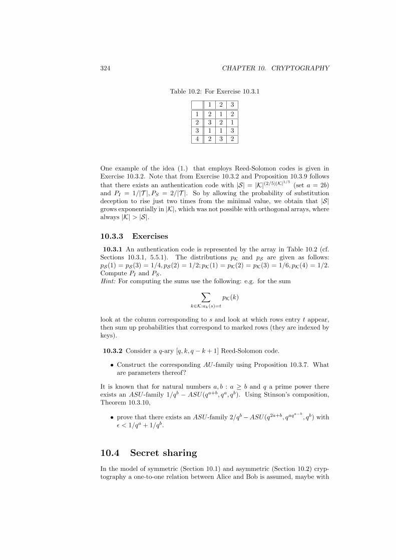
324 CHAPTER 10. CRYPTOGRAPHY
Table 10.2: For Exercise 10.3.1
1 2 3
1 2 1 22 3 2 13 1 1 34 2 3 2
One example of the idea (1.) that employs Reed-Solomon codes is given inExercise 10.3.2. Note that from Exercise 10.3.2 and Proposition 10.3.9 follows
that there exists an authentication code with |S| = |K|(2/5)|K|1/5
(set a = 2b)and PI = 1/|T |, PS = 2/|T |. So by allowing the probability of substitutiondeception to rise just two times from the minimal value, we obtain that |S|grows exponentially in |K|, which was not possible with orthogonal arrays, wherealways |K| > |S|.
10.3.3 Exercises
10.3.1 An authentication code is represented by the array in Table 10.2 (cf.Sections 10.3.1, 5.5.1). The distributions pK and pS are given as follows:pS(1) = pS(3) = 1/4, pS(2) = 1/2; pK(1) = pK(2) = pK(3) = 1/6, pK(4) = 1/2.Compute PI and PS .Hint: For computing the sums use the following: e.g. for the sum∑
k∈K:ak(s)=t
pK(k)
look at the column corresponding to s and look at which rows entry t appear,then sum up probabilities that correspond to marked rows (they are indexed bykeys).
10.3.2 Consider a q-ary [q, k, q − k + 1] Reed-Solomon code.
• Construct the corresponding AU -family using Proposition 10.3.7. Whatare parameters thereof?
It is known that for natural numbers a, b : a ≥ b and q a prime power thereexists an ASU -family 1/qb − ASU(qa+b, qa, qb). Using Stinson’s composition,Theorem 10.3.10,
• prove that there exists an ASU -family 2/qb−ASU(q2a+b, qaqa−b
, qb) withε < 1/qa + 1/qb.
10.4 Secret sharing
In the model of symmetric (Section 10.1) and asymmetric (Section 10.2) cryp-tography a one-to-one relation between Alice and Bob is assumed, maybe with
10.4. SECRET SHARING 325
a trusted party in the middle. This means that Alice and Bob have neces-sary pieces of secret information to convey the communication between them.Sometimes it is necessary to distribute this secret information among severalparticipants. Possible scenarios of such applications are: distributing the secretinformation among the participants in a way so that even if some participantslost some pieces of this secret information it is still possible to reconstruct thewhole secret; also sometimes shared responsibility is required, i.e. some actionis to be triggered only when several participants combine their secret pieces ofinformation to form the one that triggers that action. Examples of the latterone could be triggering some military action (e.g. missile launch) by severalauthorized persons (e.g a president, higher military officials) or opening a bankvault by several top-officials of a bank. In this section we consider mathematicalmeans to achieve the goal. The schemes providing such functionality are calledsecret sharing schemes. We consider in detail the first such scheme proposedby Adi Shamir in 1979. Then we also briefly demonstrate how error-correctingcodes can be used for a construction of linear secret sharing schemes.In secret sharing schemes shares are produced from the secret to be shared.These shares are then assigned to participants of the scheme. The idea is thatif several authorized participants gather in a group that is large enough theyshould be able to reconstruct the secret using knowledge of their shares. Onthe contrary if a group is too small or some outsiders decide to find out thesecret, their knowledge should not be enough to figure it out. This leads to thefollowing definition.
Definition 10.4.1 Let Si, i = 1, . . . , n be the shares that are produced fromthe secret S. Consider a collection of n participants where each participant isassigned his/her share Si. A (t, n) threshold scheme is a scheme where everygroup of t (or more) participants out of n can obtain the secret S using theirshares. On the other hand any group of less than t participants should not beable to obtain S.
We next present the Shamir’s secret sharing scheme that is a classical exampleof a (t, n) threshold scheme for any n and t ≤ n.
Algorithm 10.4.2 (Shamir’s secret sharing scheme)Set-up: taking n as input prepare the scheme for n participants
1. Choose some prime power q > n and fix a working field Fq that will beused for all the operations in the scheme.
2. Assign to the n participants P1, . . . , Pn some distinct non-zero elementsx1, . . . , xn ∈ F∗q .
Input: The threshold value t, the secret information S in some form.Output: The secret S is shared among n participants.Generation and distribution of shares:
1. Encode a secret to be shared as an element S ∈ Fq. If this is not possibleredo the Set-up phase with a larger q.
2. Choose randomly t − 1 elements a1, . . . , at−1 ∈ Fq. Assign a0 := S and
form the polynomial f(X) =∑t−1i=0 aiX
i ∈ Fq[X].
326 CHAPTER 10. CRYPTOGRAPHY
3. For i = 1, . . . , n do
• compute value yi = f(xi), i = 1, . . . , n and assign the value yi to Pi.
Computing the secret from the shares:
1. Any t participants Pi1 , . . . , Pit pull their shares yi1 , . . . , yit together andthen using e.g. Lagrange interpolation with t interpolation points (xi1 , yi1),. . . , (xit , yit) restore f and thus a0 = S = f(0).
The part ”Computing the secret from the shares” is clearly justified by thefollowing formulas of Lagrange interpolation (w.l.o.g. the first t participantspull their shares):
f(X) =
t∑i=1
yi∏j 6=i
X − xjxi − xj
,
so that f(xi) = yi, i = 1, . . . , t and f is a unique polynomial of degree ≤ t − 1with this property. Of course the participants do not have to reconstruct thewhole f , they just need to know a0 that can be computed as
S = a0 =
t∑i=1
ciyi, ci =∏j 6=i
xjxj − xi
. (10.2)
So every t or more participants can recover the secret value S = f(0). On theother hand it is possible to show that for any t − 1 shares (w.l.o.g. the firstones) (xi, yi), i = 1, . . . , t− 1 and any a ∈ Fq there exists a polynomial fa such
that its evaluation at 0 is a. Indeed, take fa(X) = a+Xfa(X), where fa(X) isthe Lagrange polynomial of degree ≤ t − 2 such that fa(xi) = (yi − a)/xi, i =1, . . . , t− 1 (recall that xi’s are non-zero). Then deg fa ≤ t− 1, fa(xi) = yi, andfa(0) = a. So this means that any t−1 (or less) participants have no informationabout S: the best they can do is to guess the value of S, the probability of sucha guess is 1/q. This is because, to their knowledge, f can be any of fa’s.
Example 10.4.3 Let us construct a (3, 6) Shamir’s threshold scheme. Takeq = 8 and fix the field F8 = F2[α]/〈α3 + α + 1〉. Element α is a generatingelement of F8
∗. For i = 1, . . . , 6 assign xi = αi to the participant Pi. Supposethat the secret S = α5 is to be shared. Choose a1 = α3, a2 = α6, so that f(X) =α5+α3X+α6X2. Now evaluate y1 = f(α) = α3, y2 = f(α2) = α3, y3 = f(α3) =α6, y4 = f(α4) = α5, y5 = f(α5) = 1, y6 = f(α6) = α6. For every i = 1, . . . , 6assign yi as a share for Pi. Now suppose that the participants P2, P3, and P5
decide to pull their shares together and obtain S. As in (10.2) they computec2 = x3
x3−x2
x5
x5−x2= 1, c3 = 1, c5 = 1. Accordingly, c2y2 + c3y3 + c5y5 = α5 = S.
On the other hand, due to the explanation above, any 2 participants cannotdeduce S from their shares. In other words, any element of F8 is equally likelyfor them to be the secret.
See Exercise 10.4.1 for a simple construction of a (t, t) threshold scheme.Next let us outline how one can use linear error-correcting codes to constructsecret sharing schemes. Let us fix the finite field Fq: the secret values will bedrawn from this field. Also consider an [n, k]q linear code C with a generatormatrix G that has g′0, . . . ,g
′n−1 as columns (we add dashes to indicate that
10.4. SECRET SHARING 327
these are columns and they are not to be confused with the usual notation forrows of G). Choose some information vector a ∈ Fkq such that S = ag′0, whereS is the secret information. Then compute s = (s0, s1, . . . , sn−1) = aG. Nows0 = S and s1, . . . , sn−1 can be used as shares. The next result characterizes asituation when the secret S can be obtained from the shares.
Proposition 10.4.4 With the notation as above, let si1 , . . . , sim be some sharesfor 1 ≤ m ≤ n − 1. These shares can reconstruct the secret S iff c⊥ =(1, 0, . . . , 0, ci1 , 0, . . . , 0, cim , 0, . . . , 0) ∈ C⊥, where at least one cij 6= 0.
Proof. The claim follows from the fact that G · c⊥T = 0 and that the secretS = ag′0 can be obtained iff g′0 is a linear combination of g′i1 , . . . ,g
′im
.
If we carefully look one more time at Shamir’s scheme it is not a surprise thatit can be seen as the above construction with Reed-Solomon code as a code C.Indeed, choose N = q−1 and set xi = αi where α is a primitive element of Fq. Itis then quite easy to see that encoding the secret and shares via the polynomialf as in Algorithm 10.4.2 is equivalent to encoding via the Reed-Solomon codeRSt(N, 1), cf. Definition 8.1.1 and Proposition 8.1.4. The only nuance is thatin general we may assign some n ≤ N shares and not all N . Now we need tosee that every collection of t shares reconstructs the secret. Using the abovenotation, let si1 , . . . , sit be the shares pulled together. According to Proposition10.4.4 the dual of C = RSt(N, 1) should contain a codeword with the 1 at thefirst position and at least one non-zero element at positions i1, . . . , it. FromProposition 8.1.2 we have that RSt(N, 1)⊥ = RSN−t(N,N) and RSN−t(N,N)is an MDS [N,N − t, t + 1] code. We use now Corollary 3.2.14 with the t + 1positions 1, i1, . . . , it and we are guaranteed to have a prescribed codeword.Therefore every collection of t shares reconstructs the secret. Having xi = αi isnot really a restriction (Exercise 10.4.3).In general the problem of constructing secret sharing schemes can be reducedto finding codewords of minimum weight in a dual code as per Proposition10.4.4. There are more advanced constructions based on error-correcting codes,in particular based on AG-code, see Notes for the references.
It is clear that if a group of participants can recover the secret by combining theirshares, then any group of participants containing this group can also recover thesecret. We call a group of participants a minimal access set, if the participantsof this group can recover the secret with their shares, while any proper subgroupof participants can not do so. From the preceding discussions, it is clear thatthere is one-to-one correspondence between the set of minimal access sets andthe set of minimal weight codewords of the dual code C⊥ whose first coordinateis 1. Therefore, for a secret sharing scheme based on a code C, the problemof determining the access structure of the secret sharing scheme is reduced tothe problem of determining the set of minimal weight codewords whose firstcoordinate is 1. It is obvious that the shares for the participants depend on theselection of the generator matrix G of the code C. However, by Proposition??, the selection of generator matrix does not affect the access structure of thesecret sharing scheme.
Note that the set of minimal weight codewords whose first coordinate is 1 is asubset of the set of all minimal weight codewords. The problem of determiningthe set of all minimal weight codewords of a code is known as the covering
328 CHAPTER 10. CRYPTOGRAPHY
problem. This problem is a hard problem for an arbitrary linear code. In thefollowing, let us have some more discussions on the access structure of secretesharing schemes based on special classes of linear codes. It is clear that for anyparticipant, he (she) must be in at least one minimal access set. This is true forany secret sharing scheme. Now, we further ask the following question: Given aparticipant Pi, how many minimal access sets are there which contain Pi? Thisquestion is solved if the dual code of the code used by the secret sharing schemeis a constant weight code. In the following proposition, we suppose C is a q-ary[n, k] code, and G = (g′0,g
′1, . . . ,g
′n−1) is a generator matrix of C.
Proposition 10.4.5 Suppose C is a constant weight code. Then, in the secretsharing scheme based on C⊥, there are qk−1 minimal access sets. Moreover, wehave the following:
(1) If g′i is a scalar multiple of g′0, 1 ≤ i ≤ n− 1, then every minimal accessset contains the participant Pi. Such a participant is called a dictatorialparticipant.
(2) If g′i is not a scalar multiple of g′0, 1 ≤ i ≤ n−1, then there are (q−1)qk−1
minimal access sets which contain the participant Pi.
Proof. .........will be given later.........
The following problem is an interesting research problem: Identify (or construct)linear codes which are good for secret sharing, that is, the covering problem canbe solved, or the minimal weight codewords can be well characterized. Severalclasses of linear codes which are good for secret sharing have been identified,see the papers by C. Ding and J. Yuan.
10.4.1 Exercises
10.4.1 Suppose that some trusted party T wants to share a secret S ∈ Zmbetween two participants A and B. For this, T generates some random numbera ∈ Zm and assigns it to A. T then assigns b = S − a mod m to B.
• Show that the scheme above is a (2, 2) threshold scheme. This scheme isan example of a split-knowledge scheme.
• Generalize the idea above to construct a (t, t) threshold scheme for arbi-trary t.
10.4.2 Construct a (4, 7) Shamir’s threshold scheme and share the bit-string”1011” using it.Hint: Represent the bit-string ”1011” as an element of a finite field with morethan 7 elements.
10.4.3 Remove the restriction on xi being equal to αi in the Reed-Solomonconstruction of Shamir’s scheme by using Proposition 3.2.10.
10.5. BASICS OF STREAM CIPHERS. LINEAR FEEDBACK SHIFT REGISTERS329
10.5 Basics of stream ciphers. Linear feedbackshift registers
In Section 10.1 we have seen how block ciphers are used for construction ofsymmetric cryptosystems. Here we give some basics of stream ciphers, i.e. ci-phers that proceed information bitwise as oppose to blockwise. Stream ciphersare usually faster than block ciphers and have lower requirements on imple-mentation costs. Nevertheless, stream ciphers appear to be more susceptible tocryptanalysis. Therefore, much care should be put in designing a secure cipher.In this section we concentrate on stream cipher design that involves the linearfeedback shift register (LFSR) as one of the building blocks.The difference between block and stream ciphers is quite vague, since a blockcipher can be turned to a stream one using some special mode of operation.Nevertheless, let us see what are characterizing features of such ciphers. Astream cipher is defined via its stream of states S, the keystream K, and thestream of outputs C. Having an input (plaintext) stream P, one would like toobtain C using S and K by operating successively on individual units of thesestreams. The streams C and K are obtained using some key, either secret ornot. If these units are binary bits, we are dealing with the binary cipher.Consider an infinite sequence (a stream) of key bits k1, k2, k3, . . . , and a streamof plaintext bits p1, p2, p3, . . . . Then we can form a ciphertext stream by sim-ply adding the key stream and the plaintext stream bitwise: ci = pi ⊕ ki, i =1, 2, 3, . . . . One can stop at some moment n thus having the n-bit ciphertextfrom the n-bit key and the n-bit plaintext. If ki’s are chosen uniformly atrandom and independently, we have the one-time pad scheme. It can be shownthat in the one-time pad if an eavesdropper only possesses the ciphertext, he/shecannot say anything about the plaintext. In other words, the knowledge of theciphertext does not shed any additional light on the plaintext for an eavesdrop-per. Moreover, an eavesdropper even knowing n key bits is completely uncertainabout the (n + 1)-th bit. This is a classical example of unconditionally securecryptosystem, cf. Definition 10.1.8.Although the above idea yields provable guarantees for security it has an es-sential drawback: a key should be at least as long as a plaintext, which is ausual thing in unconditionally secure systems, see also Section 10.3.1. Clearlythis requirement is quite impractical. That is why what is usually done is thefollowing. One starts with some bitstring of a fixed size called a seed , and thenby making some operations with this string obtains some larger string (it canbe infinite theoretically), which should “appear random” to an eavesdropper.Note that since the seed is finite we cannot talk about unconditional securityanymore, only computational. Indeed, having long enough key stream in theknown-plaintext scenario, it is in principle possible to run an exhaustive searchon all possible seeds to find out the one that gives rise to the given key stream.In particular all the successive bits of the key stream will be known.Now let us present two commonly used types of stream ciphers: synchronousand self-synchronizing. Let P = p0, p1, . . . be the plaintext stream, K =k0, k1, . . . be the keystream, C = c0, c1, . . . be the ciphertext stream, andS = s0, s1, . . . be the state stream. The synchronous stream ciphersynchronous
330 CHAPTER 10. CRYPTOGRAPHY
stream cipher is defined as follows:
si+1 = f(si, k),ki = g(si, k),ci = h(ki, pi), i = 0, 1, . . . .
Here s0 is the initial state and f is the state function, which generates a nextstate from the previous one and also depends on a key. Now ki’s form the keystream via the function g. See Exercise 10.5.1 for some toy example. Finallythe ciphertext is formed by applying the output function h to the bits ki andpi. This cipher is called synchronous, since both Alice and Bob need to usethe same key stream (ki)i. If some (non-)malicious insertions/deletions occurthe synchronization is lost, so additional means for providing synchronizationare necessary. Note that usually the function h is just a bitwise addition ofstreams (ki)i and (pi)i. It is also very common for stream ciphers to have aninitialization phase, where only the states si are updated first and the updateand output starts to happen only at some later point of time. Therewith thekey stream (ki) gets more complicated and dependent on more state bits.The self-synchronizing stream cipher is defined as
si = (ci−t, . . . , ci−1),ki = g(si, k),ci = h(ki, pi), i = 0, 1, . . . .
Here (c−t, . . . , c−1) is a non-secret initial state. So the encryption/decryptiondepends only on some number of ciphertext bits, therefore the output stream isable to recover from deletions/insertions.Observe that if h is a bitwise addition modulo 2, then the stream ciphers de-scribed above follow the idea of the one-time pad. The difference is that nowone obtains the key stream (ki)i not fully randomly, but as a pseudorandomexpansion of an initial state (seed) s0. The LFSR is used as a building blockin many stream ciphers that facilitates such a pseudorandom expansion. TheLFSRs have an advantage that they can be efficiently implemented in hardware.Also the outputs of LFSRs have nice statistical properties. Moreover, LFSRsare closely related to so-called linear recurring sequences that are readily stud-ied via algebraic methods.Schematically an LFSR can be presented as in Figure 10.3Let us figure out what is going on the diagram. First the notation. A squarebox is a delay box sometimes called ”flip-flop”. Its task is to pass its storedvalue further after each unit of time set by a synchronizing clock. A circlewith the value ai in it performs AND operation or multiplication modulo 2 onthe input with the prescribed ai. The plus sign in a circle clearly means theXOR operation or addition modulo 2. Now the square boxes are initialized withsome values, namely the box Di gets some value si ∈ 0, 1, i = 0, . . . , L − 1.When the first time unit comes to an end the following happens: the value s0
becomes an output bit. Then all values si, i = 1, . . . , L − 1 are shifted fromDi to Di−1. Simultaneously for each i = 0, . . . , L − 1 the value si goes to anAND-circle, gets multiplied with ai and then all these products are summedup by means of plus-circles, so that the sum ⊕L−1
i=0 aisi is formed. This sum iswritten to DL−1 and is called sL. The same procedure takes place at the endof the next time unit: now s1 is the output, the remaining values are shifted,
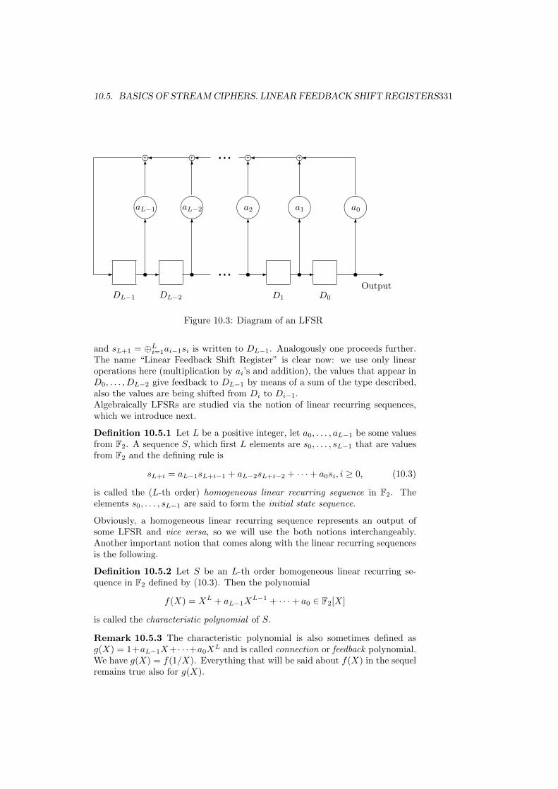
10.5. BASICS OF STREAM CIPHERS. LINEAR FEEDBACK SHIFT REGISTERS331
-
DL−1
-sDL−2
s q q q -sD1
-sD0
-sOutput
6 6 6 6
aL−1 aL−2 a2 a1
6 6 6 6
6a0
e e e e q q q
Figure 10.3: Diagram of an LFSR
and sL+1 = ⊕Li=1ai−1si is written to DL−1. Analogously one proceeds further.The name “Linear Feedback Shift Register” is clear now: we use only linearoperations here (multiplication by ai’s and addition), the values that appear inD0, . . . , DL−2 give feedback to DL−1 by means of a sum of the type described,also the values are being shifted from Di to Di−1.Algebraically LFSRs are studied via the notion of linear recurring sequences,which we introduce next.
Definition 10.5.1 Let L be a positive integer, let a0, . . . , aL−1 be some valuesfrom F2. A sequence S, which first L elements are s0, . . . , sL−1 that are valuesfrom F2 and the defining rule is
sL+i = aL−1sL+i−1 + aL−2sL+i−2 + · · ·+ a0si, i ≥ 0, (10.3)
is called the (L-th order) homogeneous linear recurring sequence in F2. Theelements s0, . . . , sL−1 are said to form the initial state sequence.
Obviously, a homogeneous linear recurring sequence represents an output ofsome LFSR and vice versa, so we will use the both notions interchangeably.Another important notion that comes along with the linear recurring sequencesis the following.
Definition 10.5.2 Let S be an L-th order homogeneous linear recurring se-quence in F2 defined by (10.3). Then the polynomial
f(X) = XL + aL−1XL−1 + · · ·+ a0 ∈ F2[X]
is called the characteristic polynomial of S.
Remark 10.5.3 The characteristic polynomial is also sometimes defined asg(X) = 1+aL−1X+ · · ·+a0X
L and is called connection or feedback polynomial.We have g(X) = f(1/X). Everything that will be said about f(X) in the sequelremains true also for g(X).
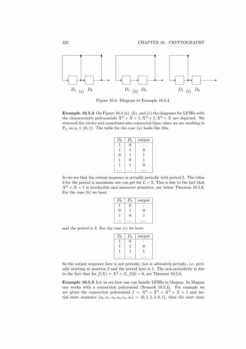
332 CHAPTER 10. CRYPTOGRAPHY
-
D1
-rD0
-r(a)
6r
6r
-
D1
-
D0
-r(b)
6r
-
D1
r-D0
-
(c)
6r
Figure 10.4: Diagram to Example 10.5.4
Example 10.5.4 On Figure 10.4 (a), (b), and (c) the diagrams for LFSRs withthe characteristic polynomials X2 + X + 1, X2 + 1, X2 + X are depicted. Weremoved the circles and sometimes also connected lines, since we are working inF2, so ai ∈ 0, 1. The table for the case (a) looks like this
D0 D1 output1 0 -1 1 00 1 11 0 11 1 0
. . . . . . . . .
So we see that the output sequence is actually periodic with period 3. The value3 for the period is maximum one can get for L = 2. This is due to the fact thatX2 + X + 1 is irreducible and moreover primitive, see below Theorem 10.5.8.For the case (b) we have
D0 D1 output1 0 -0 1 01 0 1
. . . . . . . . .
and the period is 2. For the case (c) we have
D0 D1 output1 0 -1 1 01 1 1
. . . . . . . . .
So the output sequence here is not periodic, but is ultimately periodic, i.e. peri-odic starting at position 2 and the period here is 1. The non-periodicity is dueto the fact that for f(X) = X2 +X, f(0) = 0, see Theorem 10.5.8.
Example 10.5.5 Let us see how one can handle LFSRs in Magma. In Magmaone works with a connection polynomial (Remark 10.5.3). For example weare given the connection polynomial f = X6 + X4 + X3 + X + 1 and ini-tial state sequence (s0, s1, s2, s3, s4, s5) = (0, 1, 1, 1, 0, 1), then the next state
10.5. BASICS OF STREAM CIPHERS. LINEAR FEEDBACK SHIFT REGISTERS333
(s1, s2, s3, s4, s5, s6) can be computed as> P<X>:=PolynomialRing(GF(2));
> f:=X^6+X^4+X^3+X+1;
> S:=[GF(2)|0,1,1,1,0,1];
> LFSRStep(f,S);
[ 1, 1, 1, 0, 1, 1 ]
By writing> LFSRSequence(f,S,10);
[ 0, 1, 1, 1, 0, 1, 1, 1, 1, 0 ]
we get the next 10 state values s6, . . . , s15.In Sage one can do the same in the following way> con_poly=[GF(2)(i) for i in [1,0,1,1,0,1]]
> init_state=[GF(2)(i) for i in [0,1,1,1,0,1]]
> n=10
> lfsr_sequence(con_poly, init_state, n)
[0, 1, 1, 1, 0, 1, 1, 1, 1, 0]
So one has to provide the connection polynomial via its coefficients.
As we have mentioned, the characteristic polynomial plays an essential rolein determining the properties of a linear recurring sequence and the associatedLFSR. Next we summarize all the results concerning a characteristic polynomial,but first let us make precise the notions of periodic and ultimately periodicsequences.
Definition 10.5.6 Let S = sii≥0 be a sequence such that there exists apositive integer P such that sP+i = si ∀i = 0, 1, . . . . Such a sequence is calledperiodic and P is a period of S. If the property sP+i = si holds for all i startingfrom some non-negative P0, then such a sequence is called ultimately periodicalso with a period P . Note that a periodic sequence is also ultimately periodic.
Remark 10.5.7 Note that periodic and ultimately periodic sequences havemany periods. It turns out that the least period always divides any otherperiod. We will refer to the term period meaning the least period of a sequence.
Now the main result follows.
Theorem 10.5.8 Let S be an L-th order homogeneous linear recurring se-quence and let f(X) ∈ F2[X] be its characteristic polynomial. The followingholds:
1. S is an ultimately periodic sequence with period P ≤ 2L − 1.
2. If f(0) 6= 0, then S is periodic.
3. If f(X) is irreducible over F2, then S is periodic with period n such thatP |(2L − 1).
4. If f(X) is primitive *** recall the definition? *** over F2, then S isperiodic with period P = 2L − 1.
Definition 10.5.9 A homogeneous linear recurring sequence S with f(X) aprimitive characteristic polynomial is called maximal period sequence in F2 oran m-sequence.
334 CHAPTER 10. CRYPTOGRAPHY
The notions and results above can be generalized to the case of arbitrary finitefield Fq. It is notable that one can compute the characteristic polynomial ofan L-th order homogeneous linear recurring sequence S by knowing any sub-sequence of length at least 2L by means of an algorithm by Berlekamp andMassey, which is essentially the one from Section 9.2.2 *** more details haveto be provided here to show the connection. The explanation in 9.2.2 is a bittoo technical. Maybe we should introduce a simple version of BM in Chapter6, which we could then use here? ***. See also Exercise 10.5.3.Naturally one is interested in obtaining sequences with large period. Thereforem-sequences have primary application. These sequences have nice statisticalproperties. For example the distribution of patterns that have length ≤ L is al-most uniform. The notion of linear complexity is used as a tool for investigatingthe statistical properties of outputs of LFSRs. Roughly speaking, a linear com-plexity of a sequence is a minimal L such that there exists a homogeneous linearrecurring sequence with the characteristic polynomial of degree L. Because ofnice statistical properties LFSRs can be used as pseudorandom bit generators,see Notes.An obvious cryptographic drawback of LFSRs is the fact that the whole outputsequence can be reconstructed by having just 2L bits of it, where L is the linearcomplexity of the sequence. This obstructs using LFSRs as cryptographic prim-itives, in particular as key stream generators. Nevertheless, one can use LFSRsin certain combinations, add non-linearity and obtain quite effective and se-cure key stream generators for stream ciphers. Let us briefly describe the threepossibilities of such combinations.
• Nonlinear combination generator . Here one transmits outputs of l LFSRsL1, . . . , Ll to a non-linear function f with l inputs. The output of fbecomes then the key stream. The function f should be chosen to becorrelation immune, i.e. there should be no correlation between the outputof f and outputs of any small subset of L1, . . . , Ll.
• Nonlinear filter generator . Here the L delay boxes at every time unit endgive their values to a non-linear function g with L inputs. The output ofg becomes then the key stream. The function g is chosen in a way thatits algebraic representation is dense.
• Clock-controlled generator . Here outputs of one LFSRs control the clocksof other LFSRs that compose the cipher. In this way the non-linearity isintroduced.
For some examples of the above, see Notes.
10.5.1 Exercises
10.5.1 Consider an example of a synchronous cipher defined by the followingdata. The initial state is s0 = 10010. The function f shifts its argument by 3positions to the right and adds 01110 bitwise. Now g is defined to sum up bitswith positions 2,4, and 5 modulo 2 to obtain a keystream bit. Compute the first6 key stream bits of such a cipher.
10.5.2 a. The polynomial f(X) = X4 +X3 + 1 is primitive over F2. Drawa diagram of an LFSR that has f as the characteristic polynomial. Let
10.6. PKC SYSTEMS USING ERROR-CORRECTING CODES 335
(0, 1, 1, 0) = (s0, s1, s2, s3) be the initial state. Compute the output ofsuch LFSR up to the point when it is seen that the output sequence isperiodic. What is the period?
b. Rewrite (a.) in terms of a connection polynomial. Take the same initialstate and compute (e.g. with Magma) enough output sequence values tosee the periodicity.
10.5.3 Let s0, . . . , s2L−1 be the first 2L bits of an L-th order homogeneouslinear recurring sequence defined by (10.3). If it is known that the matrix
s0 s1 . . . sL−1
s1 s2 . . . sL...
.... . .
...sL−1 sL . . . s2L−1
is invertible, show that it is possible to compute a0, . . . , aL−1, i.e. to find outthe structure of the underlying LFSR.
10.5.4 [CAS] The shrinking generator is an example of the clock-controlledgenerator. The shrinking generator is composed of two LFSR’s L1 and L2.The output of L1 controls the output of L2 in the following way: if the outputbit of L1 is one, then the output bit of L2 is taken as an output of the wholegenerator. If the output of L1 is zero, then the output of L2 is discarded. So, inother words, the output of the generator forms a subsequence of the output of L2
and this subsequence is masked by the 1’s in the output of L1. Write a procedurethat implements the shrinking generator. Then use the output of the shrinkinggenerator as a key-stream k, and define a stream cipher with it, i.e. a ciphertextis formed as ci = pi ⊕ ki, where p is the plaintext stream. Compare yoursimulation results with the ones obtained with the ShrinkingGeneratorCipherclass from Sage.
10.6 PKC systems using error-correcting codes
In this section we consider the public key encryption schemes due to McEliece(Section 10.6.1) and Niederreiter (Section 10.6.2). Both of these encryptionschemes rely on hardness of decoding random linear codes as well as hardnessof distinguishing a code with the prescribed structure from a random one. Aswe have seen, the problem of the nearest codeword decoding is NP-hard. So theMcEliece cryptosystem is one of the proposals to use an NP-hard problem as abasis, for some others see Section 10.2.3.As has been mentioned at the end of Section 10.2.1, quantum computer attacksimpose a potential threat for classical cryptosystems like RSA (Section 10.2.1)and those based on the DLP problem (Section 10.2.2). On the other side,no significant advantages of using a quantum computer in attacking the code-based schemes of McEliece and Niederreiter are known. Therefore, this area ofcryptography attracted quite a lot of attention in the last years. See Notes onthe recent developments.
336 CHAPTER 10. CRYPTOGRAPHY
10.6.1 McEliece encryption scheme
Now let us consider the public key cryptosystem by McEliece. It was proposedin 1978 and is in fact one of the oldest public key cryptosystems. The idea of thecryptosystem is to take a class of codes C for which there is an efficient boundeddistance decoding algorithm. The secret code C ∈ Cis given by a k×n generatormatrix G. This G is scrambled into G′ = SGP by means of a k × k invertiblematrix S and an n × n permutation matrix P . Denote by C ′ is the code withthe generator matrix G′. Now C ′ is equivalent to C, cf. Definition 2.5.15. Theidea of scrambling is that the code C ′ should appear random to an attacker,so it should not be possible to use the efficient decoding algorithm available forC to decrypt messages. More formally we have the following procedures thatdefine the encryption scheme as in Algorithms 10.1, 10.2, and 10.3. Note thatin these algorithms when we say “choose” we mean “choose randomly from anappropriate set”.
Algorithm 10.1 McEliece key generation
Input:System parameters:
- Length n- Dimension k- Alphabet size q- Error-correcting capacity t- A class C of [n, k] q-ary linear codes that have an efficient decoder
that can correct up to t errorsOutput: McEliece public/private key pair (PK , SK).
BeginChoose C ∈ C represented by a generator matrix G and equipped with anefficient decoder DC .Choose an invertible q-ary k × k matrix S.Choose an n× n permutation matrix P .Compute G′ := SGP a generator matrix of an equivalent [n, k] codePK := G′.SK := (DC , S, P ).return (PK , SK).End
Let us see why the decryption procedure really yields a correct message froma ciphertext. We have c1 = cP−1 = mSG + eP−1. Now since wt(eP−1) =wt(e) = t, we have c2 = DC(c1) = mS. The last step is then trivial.Initially McEliece proposed to use the class of binary Goppa codes (cf. Section8.3.2) as the class C. Interestingly enough, this class turned out to be prettymuch the only secure choice up to now. See Section 10.6.3 for the discussion.As we saw in the procedures above, decryption is just a decoding with the codegenerated by G′. So if we are successful in “masking”, for instance a binaryGoppa code C, as a random code C ′, then the adversary is faced with theproblem of correcting t errors in a random code, which is assumed to be hard,if t is large enough. More on that in Section 10.6.3. Let us consider a specificexample.
10.6. PKC SYSTEMS USING ERROR-CORRECTING CODES 337
Algorithm 10.2 McEliece encryption
Input:- Plaintext m- Public key PK = G′
Output: Ciphertext c.BeginRepresent m as a vector from Fkq .Choose randomly a vector e ∈ Fnq of weight t *** notation for these vectors?***.Compute c := mG′ + e. encode and add noise; c is of length nreturn cEnd
Algorithm 10.3 McEliece decryption
Input:- Ciphertext c- private key SK = (DC , S, P )
Output: Plaintext m.BeginCompute c1 := cP−1.Compute c2 := DC(c1).Compute c3 := c2S
−1.return c3
End
Example 10.6.1 [CAS] We use Magma to construct a McEliece encryptionscheme based on a binary Goppa code, encrypt a message with it and thendecrypt. First we construct a Goppa code of length 31, dimension 16, efficientlycorrecting 3 errors (see also Example 12.5.23):> q:=2^5;
> P<x>:=PolynomialRing(GF(q));
> g:=x^3+x+1;
> a:=PrimitiveElement(GF(q));
> L:=[a^i : i in [0..q-2]];
> C:=GoppaCode(L,g); // a [31,16,7] binary Goppa code
> C2:=GoppaCode(L,g^2);
> n:=#L; k:=Dimension(C);
Note that we had to define the code C2 generated by the square of the Goppapolynomial g. Although the two codes are equal, we need the code C2 later fordecoding. *** add references *** Now the key generation part:> G:=GeneratorMatrix(C);
> S:=Random(GeneralLinearGroup(k,GF(2)));
> Determinant(S); // indeed an invertible map
1
> p:=Random(Sym(n)); // a random permutation of an n-set
> P:=PermutationMatrix(GF(2), p); // its matrix
> GPublic:=S*G*P; // our public generator matrix
After we have obtained the public key, we can encrypt a message:
338 CHAPTER 10. CRYPTOGRAPHY
> MessageSpace:=VectorSpace(GF(2),k);
> m:=Random(MessageSpace);
> m;
(1 1 0 0 1 1 1 0 0 0 0 1 1 1 0 0)
> m2:=m*GPublic;
> e:=C ! 0; e[10]:=1; e[20]:=1; e[25]:=1; // add 3 errors
> c:=m2+e;
Let us decrypt using the private key:> c1:=c*P^-1;
> bool,c2:=Decode(C2,c1: Al:="Euclidean");
> IS:=InformationSet(C);
> ms:=MessageSpace ! [c2[i]: i in IS];
> m_dec:=ms*S^-1;
> m_dec;
(1 1 0 0 1 1 1 0 0 0 0 1 1 1 0 0)
We see that m_dec=m. Note that we applied the Euclidian algorithm for decodinga Goppa code (*** reference ***), but we had to apply it to the code generatedby g^2 to be able to correct all three errors. Since as a result of decoding weobtained a codeword, not the message it encodes, we had to find an informationset and then extract a subvector at positions that correspond to this set (ourgenerator matrices are in a standard form, so we simply take the subvector).
10.6.2 Niederreiter’s encryption scheme
The scheme proposed by Niederreiter in 1986 is dual to the one of McEliece.Namely, instead of using generator matrices and words, this scheme uses paritycheck matrices and syndromes. Although different in terms of parameter sizesand efficiency of en-/decryption, the two schemes of McEliece and Niederreiteractually can be shown to have equivalent security, see the end of this section.We now present how keys are generated and how en-/decryption is performed inthe Niederreiter scheme in Algorithms 10.4, 10.5, and 10.6. Note that in thesealgorithms we use the syndrome decoder. Recall that the notion of a syndromedecoder is equivalent to the notion of a minimum distance decoder *** add thisto the decoding section ***.The correctness of the en-/decryption procedures is shown analogously to theMcEliece scheme, see Exercise 10.6.1. The only difference is that here we usea syndrome decoder, which returns a vector with the smallest non-zero weightthat has the input syndrome, whereas in the case of McEliece the output ofa decoder is the codeword closest to the given word. Let us take a look at aspecific example.
Example 10.6.2 [CAS] We are working in Magma as in Example 10.6.1 andare considering the same binary Goppa code from there. So the first 8 lines thatdefine the code are the same; we just add> t:=Degree(g);
Now the key generation part is quite similar as well:> H:=ParityCheckMatrix(C);
> S:=Random(GeneralLinearGroup(n-k,GF(2)));
> p:=Random(Sym(n));P:=PermutationMatrix(GF(2), p);
> HPublic:=S*H*P; // our public parity check matrix
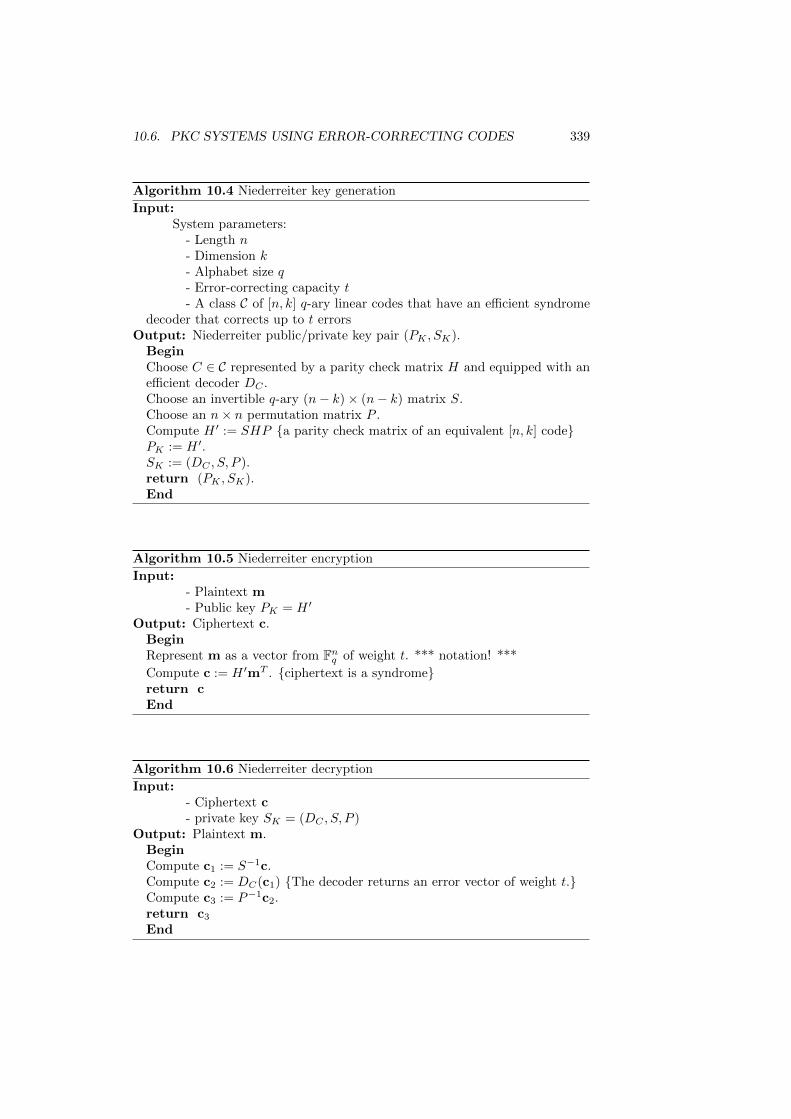
10.6. PKC SYSTEMS USING ERROR-CORRECTING CODES 339
Algorithm 10.4 Niederreiter key generation
Input:System parameters:
- Length n- Dimension k- Alphabet size q- Error-correcting capacity t- A class C of [n, k] q-ary linear codes that have an efficient syndrome
decoder that corrects up to t errorsOutput: Niederreiter public/private key pair (PK , SK).
BeginChoose C ∈ C represented by a parity check matrix H and equipped with anefficient decoder DC .Choose an invertible q-ary (n− k)× (n− k) matrix S.Choose an n× n permutation matrix P .Compute H ′ := SHP a parity check matrix of an equivalent [n, k] codePK := H ′.SK := (DC , S, P ).return (PK , SK).End
Algorithm 10.5 Niederreiter encryption
Input:- Plaintext m- Public key PK = H ′
Output: Ciphertext c.BeginRepresent m as a vector from Fnq of weight t. *** notation! ***
Compute c := H ′mT . ciphertext is a syndromereturn cEnd
Algorithm 10.6 Niederreiter decryption
Input:- Ciphertext c- private key SK = (DC , S, P )
Output: Plaintext m.BeginCompute c1 := S−1c.Compute c2 := DC(c1) The decoder returns an error vector of weight t.Compute c3 := P−1c2.return c3
End
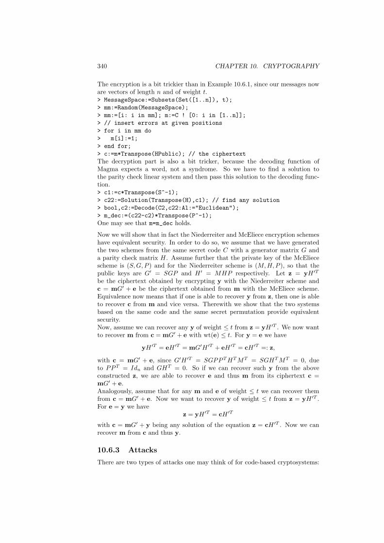
340 CHAPTER 10. CRYPTOGRAPHY
The encryption is a bit trickier than in Example 10.6.1, since our messages noware vectors of length n and of weight t.> MessageSpace:=Subsets(Set([1..n]), t);
> mm:=Random(MessageSpace);
> mm:=[i: i in mm]; m:=C ! [0: i in [1..n]];
> // insert errors at given positions
> for i in mm do
> m[i]:=1;
> end for;
> c:=m*Transpose(HPublic); // the ciphertext
The decryption part is also a bit tricker, because the decoding function ofMagma expects a word, not a syndrome. So we have to find a solution tothe parity check linear system and then pass this solution to the decoding func-tion.> c1:=c*Transpose(S^-1);
> c22:=Solution(Transpose(H),c1); // find any solution
> bool,c2:=Decode(C2,c22:Al:="Euclidean");
> m_dec:=(c22-c2)*Transpose(P^-1);
One may see that m=m_dec holds.
Now we will show that in fact the Niederreiter and McEliece encryption schemeshave equivalent security. In order to do so, we assume that we have generatedthe two schemes from the same secret code C with a generator matrix G anda parity check matrix H. Assume further that the private key of the McEliecescheme is (S,G, P ) and for the Niederreiter scheme is (M,H,P ), so that thepublic keys are G′ = SGP and H ′ = MHP respectively. Let z = yH ′T
be the ciphertext obtained by encrypting y with the Niederreiter scheme andc = mG′ + e be the ciphertext obtained from m with the McEliece scheme.Equivalence now means that if one is able to recover y from z, then one is ableto recover c from m and vice versa. Therewith we show that the two systemsbased on the same code and the same secret permutation provide equivalentsecurity.Now, assume we can recover any y of weight ≤ t from z = yH ′T . We now wantto recover m from c = mG′ + e with wt(e) ≤ t. For y = e we have
yH ′T = eH ′T = mG′H ′T + eH ′T = cH ′T =: z,
with c = mG′ + e, since G′H ′T = SGPPTHTMT = SGHTMT = 0, dueto PPT = Idn and GHT = 0. So if we can recover such y from the aboveconstructed z, we are able to recover e and thus m from its ciphertext c =mG′ + e.Analogously, assume that for any m and e of weight ≤ t we can recover themfrom c = mG′ + e. Now we want to recover y of weight ≤ t from z = yH ′T .For e = y we have
z = yH ′T = cH ′T
with c = mG′ + y being any solution of the equation z = cH ′T . Now we canrecover m from c and thus y.
10.6.3 Attacks
There are two types of attacks one may think of for code-based cryptosystems:
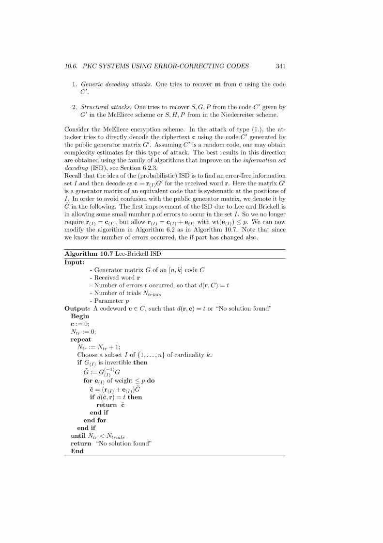
10.6. PKC SYSTEMS USING ERROR-CORRECTING CODES 341
1. Generic decoding attacks. One tries to recover m from c using the codeC ′.
2. Structural attacks. One tries to recover S,G, P from the code C ′ given byG′ in the McEliece scheme or S,H, P from in the Niederreiter scheme.
Consider the McEliece encryption scheme. In the attack of type (1.), the at-tacker tries to directly decode the ciphertext c using the code C ′ generated bythe public generator matrix G′. Assuming C ′ is a random code, one may obtaincomplexity estimates for this type of attack. The best results in this directionare obtained using the family of algorithms that improve on the information setdecoding (ISD), see Section 6.2.3.Recall that the idea of the (probabilistic) ISD is to find an error-free informationset I and then decode as c = r(I)G
′ for the received word r. Here the matrix G′
is a generator matrix of an equivalent code that is systematic at the positions ofI. In order to avoid confusion with the public generator matrix, we denote it byG in the following. The first improvement of the ISD due to Lee and Brickell isin allowing some small number p of errors to occur in the set I. So we no longerrequire r(I) = c(I), but allow r(I) = c(I) + e(I) with wt(e(I)) ≤ p. We can nowmodify the algorithm in Algorithm 6.2 as in Algorithm 10.7. Note that sincewe know the number of errors occurred, the if-part has changed also.
Algorithm 10.7 Lee-Brickell ISD
Input:- Generator matrix G of an [n, k] code C- Received word r- Number of errors t occurred, so that d(r, C) = t- Number of trials Ntrials- Parameter p
Output: A codeword c ∈ C, such that d(r, c) = t or “No solution found”Beginc := 0;Ntr := 0;repeatNtr := Ntr + 1;Choose a subset I of 1, . . . , n of cardinality k.if G(I) is invertible then
G := G(−1)(I) G
for e(I) of weight ≤ p do
c = (r(I) + e(I))Gif d(c, r) = t then
return cend if
end forend if
until Ntr < Ntrialsreturn “No solution found”End
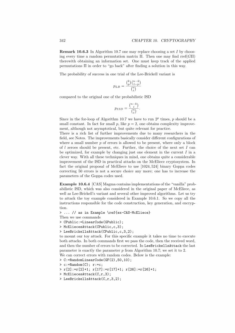
342 CHAPTER 10. CRYPTOGRAPHY
Remark 10.6.3 In Algorithm 10.7 one may replace choosing a set I by choos-ing every time a random permutation matrix Π. Then one may find rref(GΠ)therewith obtaining an information set. One must keep track of the appliedpermutations Π in order to “go back” after finding a solution in this way.
The probability of success in one trial of the Lee-Brickell variant is
pLB =
(kp
)(n−kt−p)(
nt
)compared to the original one of the probabilistic ISD
pISD =
(n−kt
)(nt
) .
Since in the for-loop of Algorithm 10.7 we have to run 2p times, p should be asmall constant. In fact for small p, like p = 2, one obtains complexity improve-ment, although not asymptotical, but quite relevant for practice.There is a rich list of further improvements due to many researchers in thefield, see Notes. The improvements basically consider different configurations ofwhere a small number p of errors is allowed to be present, where only a blockof l zeroes should be present, etc. Further, the choice of the next set I canbe optimized, for example by changing just one element in the current I in aclever way. With all these techniques in mind, one obtains quite a considerableimprovement of the ISD in practical attacks on the McEliece cryptosystem. Infact the original proposal of McEliece to use [1024, 524] binary Goppa codescorrecting 50 errors is not a secure choice any more; one has to increase theparameters of the Goppa codes used.
Example 10.6.4 [CAS] Magma contains implementations of the “vanilla” prob-abilistic ISD, which was also considered in the original paper of McEliece, aswell as Lee-Brickell’s variant and several other improved algorithms. Let us tryto attack the toy example considered in Example 10.6.1. So we copy all theinstructions responsible for the code construction, key generation, and encryp-tion.> ... // as in Example \refex-CAS-McEliece
Then we use commands> CPublic:=LinearCode(GPublic);
> McEliecesAttack(CPublic,c,3);
> LeeBrickellsAttack(CPublic,c,3,2);
to mount our toy attack. For this specific example it takes no time to executeboth attacks. In both commands first we pass the code, then the received word,and then the number of errors to be corrected. In LeeBrickellsAttack the lastparameter is exactly the parameter p from Algorithm 10.7; we set it to 2.We can correct errors with random codes. Below is the example:> C:=RandomLinearCode(GF(2),50,10);
> c:=Random(C); r:=c;
> r[2]:=r[2]+1; r[17]:=r[17]+1; r[26]:=r[26]+1;
> McEliecesAttack(C,r,3);
> LeeBrickellsAttack(C,r,3,2);
10.6. PKC SYSTEMS USING ERROR-CORRECTING CODES 343
Apart from decoding being hard for the public code C ′, it should be impossibleto deduce the structure of the code C from the public C ′. Structural attacksof (2.) aim at exploiting this structure. As we have mentioned, the choice ofbinary Goppa codes turned out to be pretty much the only secure choice upto now. There were quite a few attempts to propose other classes of codes forwhich efficient decoding algorithms are known. Alas, all of these proposals werebroken, we just name a few: Generalized Reed-Solomon (GRS) codes, Reed-Muller codes, BCH codes, algebraic-geometry codes of small genus, LDPC codes,quasi-cyclic codes; see Notes. In the next section we will consider in detail howa prominent attack on GRS works. In particular, weakness of the GRS codessuggest, due to equivalent security, the weakness of the original proposal ofNiederreiter, who suggested to use these codes in his scheme.
10.6.4 The attack of Sidelnikov and Shestakov
Let C be the code GRSk(a,b), where a consists of n mutually distinct entriesof Fq and b consists of nonzero entries, cf. Definition 8.1.10. If this code is usedin the McEliece PKC, then for an attacker the code C ′ with generator matrixG′ = SGP is known, where S is an invertible k × k matrix and P = ΠD withΠ an n× n permutation matrix and D an invertible diagonal matrix. The codeC ′ is equal to GRSk(a′,b′), where a′ = aΠ and b′ = bP . In order to decodeGRSk(a′,b′) up to b(n − k + 1)/2c errors it is enough to find a′ and b′. TheS is not essential in masking G, since G′ has a unique row equivalent matrix(Ik|A′) that is in reduced row echelon form. Here A′ is a generalized Cauchymatrix (Definition 3.2.17), but it is a priori not evident how to recover a′ andb′ from this.
The code is MDS hence all square submatrices of A′ are invertible by Re-mark 3.2.16. In particular all entries of A′ are nonzero. After multiplyingthe coordinates with nonzero constants we get a code which is generalizedequivalent with the original one, and is again of the form GRSk(a′′,b′′), sincer ∗ GRSk(a′,b′) = GRSk(a′,b′ ∗ r). So without loss of generality it may beassumed that the code has a generator matrix of the form (Ik|A′) such that thelast row and the first column of A′ consists of ones.Without loss of generality it may be assumed that ak−1 = ∞, ak = 0 andak+1 = 1 by Proposition 8.1.25. Then according to Proposition 8.1.17 andCorollary 8.1.19 there exists a vector c with entries ci given by
ci =
b′i∏kt=1,t6=i(a
′i − a′t) if 1 ≤ i ≤ k,
b′i∏kt=1(a′i − a′t) if k + 1 ≤ i ≤ n,
such that A′ has entries a′ij given by
a′ij =cj+k−1c
−1i
a′j+k−1 − a′ifor 1 ≤ i ≤ k − 1, 1 ≤ j ≤ n− k + 1 and
a′ik = cj+k−1c−1i
for 1 ≤ j ≤ n− k + 1.
344 CHAPTER 10. CRYPTOGRAPHY
Example 10.6.5 Let G′ be the generator matrix of a code C ′ with entries inF7 given by
G′ =
6 1 1 6 2 2 33 4 1 1 5 4 31 0 3 3 6 0 1
.
Then rref(G′) = (I3|A′) with
A′ =
1 3 3 64 4 6 63 1 6 3
.
G′ is a pubic key and it is known that it is the generator matrix of a generalizedReed-Solomon code. So we want to find a in F7
7 consisting of mutually distinctentries and b in F7
7 with nonzero entries such that C ′ = GRS3(a,b). NowC = (1, 4, 3, 1, 5, 5, 6) ∗ C ′ has a generator matrix of the form (I3|A) with
A =
1 1 1 11 5 4 21 4 3 6
.
We may assume without loss of generality that a1 = 0 and a2 = 1 by Proposition8.1.25. ***...............***
10.6.5 Exercises
10.6.1 Show the correctness of the Niederreiter scheme.
10.6.2 Using methods of Section 10.6.3 attack larger McEliece schemes. Inthe Goppa construction take
- m = 8, r = 16
- m = 9, r = 5
- m = 9, r = 7
Make observations that would answer the following questions:
- Which attack is faster: the plain ISD or Lee-Brickell’s variant?
- What is the role of the parameter p? What is the optimal value of p inthese experiments?
- Does the execution time differ from one run to the other or it stays thesame?
- Is there any change in execution time, when the attacks are done forrandom codes with the same parameters as above?
Try to experiment with other attack methods implemented in Magma: LeonsAttack,SternsAttack, CanteautChabaudsAttack.Hint: For constructing Goppa polynomials use the command PrimitivePolynomial.
10.7. NOTES 345
10.6.3 Consider binary Goppa codes of length 1024 and Goppa polynomial ofdegree 50.(1) Give an upper bound of the number of these codes.(2) What is the fraction of the number of these codes with respect to all binary[1024, 524] codes?(3) What is the minimum distance of a random binary [1024, 524] code accordingto the Gilbert-Varshamov bound?
10.6.4 Give an estimate of the complexity of decoding 50 errors of a receivedword with respect to a binary [1024, 524, 101] code by means of covering setdecoding.
10.6.5 Let α ∈ F8 be a primitive element such that α3 = α+ 1. Let G′ be thegenerator matrix given by
G′ =
α6 α6 α 1 α4 1 α4
0 α3 α3 α4 α6 α6 α4
α4 α5 α3 1 α2 0 α6
.
(1) Find a in F78 consisting of mutually distinct entries and b in F7
8 with nonzeroentries such that G′ is a generator matrix of GRS3(a,b).(2) Consider the 3 × 7 generator matrix G of the code RS3(7, 1) with entryα(i−1)(j−1) in the i-th row and the j-th column. Give an invertible 3× 3 matrixS and a permutation matrix P such that G′ = SGP .(3) What is the number of pairs (S, P ) of such matrices?
10.7 Notes
Some excellent references for introduction to cryptography are [87, 117, 35].
10.7.1 Section 10.1
Computational security concerns with practical attacks on cryptosystems, whereas un-
conditional security works with probabilistic models, where an attacker is supposed
to possess unlimited computing power. A usual claim when working with uncondi-
tional security would be to give an upper bound of attacker’s success probability. This
probability is independent on the computing power of an attacker and bears ”absolute
value”. For instance in the case of Shamir’s secret sharing scheme (Section 10.4) no
matter how much computing power does a group of t − 1 participants have, it does
not have better to do as to guess a value of the secret. Probability of such a success
is 1/q. More on these issues can be found in [117].
A couple of remarks on block ciphers that were used in the past. Jefferson cylinder
invented by Thomas Jefferson in 1795 and independently by Etienne Bazeries is a
polyalphabetic cipher used by the U.S. army in 1923-1942 and had the name M-94.
It was constructed as a rotor with 20–36 discs with letters, each of which provided a
substitution at a corresponding position. For its time it had quite good cryptographic
properties. Probably the best known historic cipher is German’s Enigma. It had been
used for commercial purposes already in 1920s, but became famous for its use during
the World War II by the Nazi German military. Enigma is also a rotor-based polyal-
phabetic cipher. More on historical ciphers in [87].
346 CHAPTER 10. CRYPTOGRAPHY
The Kasiski method aims at recovering period of a polyalphabetic substitution cipher.
Here one encrypts repeated portions of a plaintext with the same keyword. More de-
tails in [87].
The National Bureau of Standards (NBS, later became National Institute of Standards
and Technology - NIST) initiated development of DES (Data Encryption Standard) in
early 1970s. IBM’s cryptography department and in particular its leaders Dr. Horst
Feistel (recall Feistel cipher) and Dr.W.Tuchman contributed the most to the devel-
opment. The evaluation process was also facilitated by the NSA (National Security
Agency). The standard was finally approved and published in 1977 [90]. A lot of
controversy accompanied DES since its appearance. Some experts claimed that the
developers could have intentionally added some design trapdoors to the cipher, so
that its cryptanalysis would have been possible by them, but not by the others. The
key size 56-bits also raised concern, which eventually led to the need to adopt a new
standard. Historical remarks on DES and its development can be found in [112].
Differential and linear cryptanalysis turned out to be the most successful theoretical at-
tacks on DES. For initial papers on these attacks, see [15, 82]. The reader may also visit
http://www.ciphersbyritter.com/RES/DIFFANA.HTM for more references and history
of the differential cryptanalysis. We also mention that differential cryptanalysis may
have been known to the developers long before Adi Shamir published his paper in
1990.
Since DES encryptions do not form a group, the use of a triple application of DES
was proposed that was called triple DES [66]. Although no effective cryptanalysis
against triple DES was proposed it is barely used due to its slow compared to AES
implementation.
In the middle of 1990s it became apparent to the cryptography community that the
DES did not provide sufficient security level anymore. So NIST announced a competi-
tion for a cipher that would replace DES and became the AES (Advanced Encryption
Standard). The main criteria that were imposed for the future AES were resistance
to linear and differential cryptanalysis, faster and more effective (compared to DES)
implementation, ability to work with 128-bit plaintext blocks and 128, 192, 256-bit
keys; the number of rounds was not specified. After five years of the selection process,
the cipher Rijndael proposed by the Belgian researchers Joan Daemen and Vincent
Rijmen won. The cipher was officially adopted for the AES in 2001 [91]. Because
resistance to linear and differential cryptanalysis was one of the milestones in the
design of AES, J.Daemen and V.Rijmen carefully studied this question and showed
how such resistance can be achieved within Rijndael. In the design they used what
they called wide trail strategy - a method devised specifically to counter the linear
and differential cryptanalysis. Description of the AES together with the discussion
of underlying design decisions and theoretical discussion can be found in [45]; for the
wide trail strategy see [46].
As to attacks on AES, up to now there is no attack out there that could break AES
at least theoretically, i.e. faster than the exhaustive search, in a scenario where the
unknown key stays the same. Several attacks, though, work on non-full AES that
performs less than 10 rounds. For example Boomerang type of attacks are able to
break 5–6 rounds of AES-128 much faster, than the exhaustive search. For 6 rounds
the Boomerang attack has data complexity of 271 128-bit blocks, memory complexity
of 233 blocks and time complexity of 271 AES encryptions. This attack is mounted
under a mixture of chosen plaintext and adaptive chosen ciphertext scenarios. Some
other attacks also can attack 5–7 rounds. Among them are the Square attack, pro-
posed by Daemen and Rijmen themselves, collision attack, partial sums, impossible
10.7. NOTES 347
differentials. For an overview of attacks on Rijndael see [40]. There are recent works
on related key attacks on AES, see [1]. It is possible to attack 12 rounds of AES-192
and 14 rounds of AES-256 in the related key scenario. Still, it is quite questionable
by the community on whether one may consider these as a real threat.
We would like to mention several other recent block ciphers. The cipher Serpent is an
instance of an SP-network and was the second in the AES competition that was won
by Rijndael. As was prescribed by the selection committee it also operates on 128-bit
blocks and key of sizes 128, 192, and 256 bits. Serpent has a strong security margin,
prescribing 32 rounds. Some information online: http://www.cl.cam.ac.uk/~rja14/
serpent.html. Next, the cipher Blowfish proposed in 1993 is an instance of a Feis-
tel cipher, has 16 rounds and operates on 64-bit blocks and default key size of 128
bits. Blowfish is up to now resistant to cryptanalysis and its implementation is rather
fast, although has some limitations that preclude its use in some environments. Infor-
mation online: http://www.schneier.com/blowfish.html. A successor of Blowfish
proposed by the same person - Bruce Schneier - Twofish was one of the five finalists
in the AES competition. It has the same block and key sizes as all the AES contes-
tants and has 16 rounds. Twofish is also a Feistel cipher. This cipher is also believed
to resist cryptanalysis. Information online http://www.schneier.com/twofish.html.
It is noticeable that all these ciphers are in public domain and are free for use
in any software/hardware implementations. A light-weight block cipher PRESENT
that operates on plaintext block of only 64 bits and key length of 80 and 128 bits;
PRESENT has 31 rounds [2]. There exist proposals with even smaller block lengths,
see http://www.ecrypt.eu.org/lightweight/index.php/Block_ciphers.
10.7.2 Section 10.2
The concept of the asymmetric cryptography was introduced by Diffie and Hellman
in 1976 [48]. For an introduction to the subject and survey of results see [87, 89]. The
notion of a one-way as well as trapdoor one-way function was also introduced by Diffie
and Hellman in the same paper [48].
Rabin’s scheme from Example 10.2.2 was introduced by Rabin in [97] in 1979 and
ElGamal scheme was presented in [55]. The notion of a digital signature was also
presented in the pioneering work [48], see also [88].
The RSA scheme was introduced in 1977 by Rivest, Shamir, and Adleman [100]. In
the same paper they showed that computing the decryption exponent and factoring
are equivalent. There is no known polynomial time algorithm for factoring integers.
Still there are quite a few algorithms out there that have sub-exponential complex-
ity. For a survey of existing methods, see [96]. Asymptotically the best known sub-
exponential algorithm is general number field sieve, and it has an expected running
time of O(exp(( 649b)1/3 log b2/3)), where b is a bit length of a number n that is to be
factored [36].
Development of factoring algorithms changed requirements on the RSA key size through
the time. In their original paper [100] the authors suggested the use of 200 decimal
digit modulus (664 bits). The sizes of 336 and 512 bits were also used. In 2010 the
result of factoring RSA-768 was announced. Used at present modulus of 1024 bits
raises many questions on whether it may be considered secure. Therefore, for long-
term security the key size of 2048 or even 3072 bits are to be used. Quite remarkable is
the work of Shor [?, ?] who proposed an algorithm that can solve integer factorization
problem in polynomial time on a quantum computer.
The use of Z∗n in ElGamal scheme was proposed in [83]. For the use of Jacobian of
348 CHAPTER 10. CRYPTOGRAPHY
a hyperelliptic curve see [41]. There are several methods for solving DLP, we name
just a few: Baby-step giant-step, Pollard’s rho and Pollard’s lambda (or kangaroo),
Pohlig-Hellman, index calculus. The fastest algorithms for solving DLP for Z∗p and
F2m are variations of the index calculus algorithm. All of the above algorithms ap-
plied to the multiplicative group of a finite field do not have polynomial complexity.
For an introduction to these methods the reader may consult [41]. Index calculus is
an algorithm with sub-exponential complexity. These developments on DLP solving
algorithms affected the key size of El Gamal scheme. In practice the key size grew
from 512 to 768 and finally to 1024. At the moment using 1024-bit key for El Gamal
is considered to be a standard. The mentioned work of Shor [108] also solve the DLP
problem in polynomial time. Therefore existence of a large enough quantum computer
jeopardizes the ElGamal scheme.
Despite doubts of some researcher of a possibility to construct a large enough quan-
tum computer, the area of post-quantum cryptography has evolved that incorporates
cryptosystems that are potentially resistant to quantum computer attacks. See [12]
for an overview of the area, which includes lattice basedd, hash based, coding based,
and multivariate based cryptography. Some references to multivariate asymmetric sys-
tems, digital schemes, and their cryptanalysis can be found in [49].
The knapsack cryptosystem by Merkle and Hellman has an interesting history. It
was one of the first asymmetric cryptosystems. Its successful cryptanalysis showed
that only reliance on hardness of the underlying problem may be misleading. For an
interesting historical development, see the survey chapter of Diffie [47].
10.7.3 Section 10.3
Authentication codes were initially proposed by MacWilliams, Gilbert, and Sloan [58].
Introductory material on authentication codes is well exposed in [117].
Message authentication codes (MACs) are widely used in practice for authentication
purposes. MACs are keyed hash functions. In the case of MACs one demands from
a hash function to provide compression (a message of arbitrary size is mapped to a
fixed size vector), ease of computation (it should be easy to compute an image know-
ing the key), and computation-resistance (practical impossibility to compute an image
without knowing the key, even having some pairs element-image in disposal). More
on MACs in [87].
Results and discussion of the relation between authentication codes and orthogonal
arrays is in [117, 116, 115]. Proposition 10.3.7 is due to Bierbrauer, Johansson, Kaba-
tianskii, and Smeets [13]. By adding linear structure to the source state set, key space,
tag space, and authentication mappings one obtains linear authentication codes that
can be used in the study of distributed authentication systems [103].
10.7.4 Section 10.4
The notion of a secret sharing scheme was first introduced in 1979 by Shamir [106] and
independently by Blakely [22]. We mention here some notions that were not mentioned
in the main text. A secret sharing scheme is called perfect if knowledge of shares from
an unauthorized group (e.g. a group of < t participants in Shamir’s scheme) does not
reduce the uncertainty about the secret itself. In terms of entropy function it can be
stated like this: H(S|A) = 0, where S is the secret and A is an unauthorized set,
moreover we have H(S|B) = H(S) for B being an authorized set. In perfect secret
sharing schemes it holds that the size of each share is at least the size of the secret.
10.7. NOTES 349
If equality holds such a system is called ideal . The notion of a secret sharing scheme
can be generalized via the notion of an access structure. Using access structures one
prescribes which subsets of participants can reconstruct the secret (authorized subset)
and which cannot (unauthorized subset). The notion of a distribution of shares can
also be formalized. More details on these notions and treatment using probability
theory can be found e.g. in [117].
McEliece and Sarwate [85] were the first to point out the connection between Shamir’s
scheme and the Reed-Solomon codes construction. Some other works on relations
between coding theory and secret sharing schemes include [70, 81, 94, 138]. More
recent works concern applications of AG-codes to this subject. We mention the chapter
of Duursma [52] and the work of Chen and Cramer [39]. In the latter two references
the reader can also find the notion of secure multi-party computation, see [137]. The
idea here is that several participants wish to compute the value of some publicly known
function evaluated at their values (like shares in the above). The thing is that each
of the participants should not be able to know the values of other participants by the
known computed value of the public function and his/her own value. We also mention
that as was the case with authentication codes, information theoretic perfectness can
be traded off to obtain a system where shares are smaller than the secret [23].
10.7.5 Section 10.5
Introductory material on LFSRs with discussion of practical issues can be found in
[87]. The notion of linear complexity is treated in [102], see also materials online at
http://www.ciphersbyritter.com/RES/LINCOMPL.HTM. A thorough exposure of linear
recurring sequences is in [74].
Some examples of non-cryptographic use of LFSRs, namely randomization in digital
broadcasting: Advanced Television Systems Committee (ATSC) standard for digital
television format (http://www.atsc.org/guide_default.html), Digital Audio Broad-
casting (DAB) digital radio technology for broadcasting radio stations, Digital Video
Broadcasting - Terrestrial (DVB-T) is the European standard for the broadcast trans-
mission of digital terrestrial television (http://www.dvb.org/technology/standards/).
An example of nonlinear combination generator: E0 is a stream cipher used in the Blue-
tooth protocol, see e.g. [64]; of nonlinear filter generator Knapsack generator [87]; of
clock-controlled generators: A5/1 and A5/2 are stream ciphers used to provide voice
privacy in the Global System for Mobile communications (GSM) cellular telephone pro-
tocol http://web.archive.org/web/20040712061808/www.ausmobile.com/downloads/
technical/Security+in+the+GSM+system+01052004.pdf.
10.7.6 Section 10.6
***

350 CHAPTER 10. CRYPTOGRAPHY
Chapter 11
The theory of Grobnerbases and its applications
Stanislav Bulygin
In this chapter we deal with methods in coding theory and cryptology basedon polynomial system solving. As the main tool for this we use the theoryof Grobner bases that is a well-established instrument in computational alge-bra. In Section 11.1 we give a brief overview of the topic of polynomial systemsolving. We start with relatively easy methods of linearization and extendedlinearization. Then we give basics of more involved theory of Grobner bases.The problem we are dealing with in this chapter is the problem of polynomialsystem solving. We formulate this problem as follows: let F be a field and letP = F[X1, . . . , Xn] be a polynomial ring over F in n variables X = (X1, . . . , Xn).Let f1, . . . , fm ∈ P . We are interested in finding a set of solutions S ⊆ Fn tothe polynomial system defined as
f1(X1, . . . , Xn) = 0,
. . .
fm(X1, . . . , Xn) = 0. (11.1)
In other words, S is composed of those elements from Fn that satisfy all theequations above.In terms of algebraic geometry this problem may be formulated as follows. Givenan ideal I ⊆ P , find the variety VF(I) which it defines:
VF(I) = x = (x1, . . . , xn) ∈ Fn|f(x) = 0 ∀f ∈ I.
Since now we are interested in applications to coding and cryptology, we willbe working over finite fields and often we would like solutions of correspondingsystems to lie in these finite fields, rather than in an algebraic closure. Recallthat for every element α ∈ Fq the following holds: αq = α. This means that ifwe add an equation Xq −X = 0 to a polynomial system (11.1), we are guaran-teed that solutions for the X-variable lie in Fq.After introducing tools for the polynomial system solving in Section 11.1, we
351
352CHAPTER 11. THE THEORY OF GROBNER BASES AND ITS APPLICATIONS
give two concrete applications in Sections 11.2 and 11.3. In Section 11.2 we con-sider applications of Grobner bases techniques to decoding linear codes, whereasSection 11.3 deals with methods of algebraic cryptanalysis of block ciphers. Dueto space limitations many interesting topics related to these areas are not con-sidered. We provide their short overview with references in the Notes section.
11.1 Polynomial system solving
11.1.1 Linearization techniques
We know how to solve systems of linear equations efficiently. Gaussian elimi-nation is a standard tool for this job. If we are given a system of non-linearequations, a natural solution would be to try to reduce this problem to a lin-ear one, which we know how to solve. This simple idea leads to a techniquethat is called linearization. This technique works as follows: we replace everymonomial occurring in a non-linear (polynomial) equation by a new variable.At the end we obtain a linear system with the same number of equations, butmany new variables. The hope is that by solving this linear system we are ableto get a solution to our initial non-linear problem. It is better to illustrate thisapproach on a concrete example.
Example 11.1.1 Consider a quadratic system in two unknowns x and y overthe field F3:
x2 − y2 − x+ y = 0−x2 + x− y + 1 = 0y2 + y + x = 0x2 + x+ y = 0
Introduce new variables a := x2 and b := y2. Therewith we have a linear system:a− b− x+ y = 0−a+ x− y + 1 = 0b+ y + x = 0a+ x+ y = 0
This system has a unique solution, which may be found with the Gaussianelimination: a = b = x = y = 1. Moreover, the solution on a and b is consistentwith the conditions a = x2, b = y2. So although the system is quadratic, we arestill able to solve it purely with methods of linear algebra.
It must be noted that the linearization technique works very seldom. Usuallythe number of variables (i.e. monomials) in the system is much lager than thenumber of equations. Therefore one has to solve an underdetermined linearsystem, which has many solutions, among which it is hard to find a “real” onethat stems from the original non-linear system.
Example 11.1.2 Consider a system in three variables x, y, z over the field F16: xy + yz + xz = 0xyz + x+ 1 = 0xy + y + z = 0
11.1. POLYNOMIAL SYSTEM SOLVING 353
It may be shown that over F16 this system has a unique solution (1, 0, 0). If wereplace monomials in this system with new variables we will end up with a linearsystem of 3 equations and 7 variables. This system is full rank. In particular thevariables x, y, z are now free variables which yield values for other variables. Sosuch linear system has 163 solutions, of which only one will provide a legitimatesolution for the initial system. Other solutions do not have any meaning. E.g.we may show that assignment x = 1, y = 1, z = 1 implies that “variable” xyshould be 0, and of course this cannot be true, since both x and y are 1. So usinglinearization technique boils down to sieving the set F3
16 for a right solution, butthis is nothing more than an exhaustive search for the initial system.
So the problem with the linearization technique is that we do not have enoughlinearly independent equations for solving. Here is where the idea of eXtendedLinearization (XL) comes in hand. The idea of XL is to multiply initial equa-tions by all monomials up to given degree (hopefully not too large) to generatenew equations. Of course new variables will appear, since new monomials willappear. Still if the system is “nice” enough we may generate necessary numberof linearly independent equations to obtain a solution. Namely, we hope thatafter “extending” our system with new equations and doing Gaussian elimina-tion, we will be able to find a univariate equation. Then we can solve it andplug in obtained values and then proceed with a simplified system.
Example 11.1.3 Consider a small system in two unknowns x, y over the fieldF4:
x2 + y + 1 = 0xy + y = 0
It is clear that the linearization technique does not work so well in this case,since the number of variables (3) is larger than the number of equations (2).Now multiply the two equations first with x and then with y. Therewith weobtain four new equations, which have the same solution as the initial ones, sowe may add them to the system. The new equations are:
x3 + xy + x = 0x2y + xy = 0x2y + y2 + y = 0xy2 + y2 = 0
Here again the number of equations is lower than the number of variables. Still,by ordering monomials in the way that y2 and y go leftmost in the matrixrepresentation of a system and doing Gaussian elimination, we encounter aunivariate equation y2 = 0 (check this!). So we have a solution for y, namelyy = 0. After substituting y = 0 in the first equation we have x2 + 1 = 0, whichis again a univariate equation. Over F4 is has a unique solution x = 1. So byusing linear algebra and univariate equation solving, we were able to obtain thesolution (1, 0) for the system.
Algorithm 11.1 explains more formally how the XL works. In our example itwas enough to set D = 3. Usually one has to go much higher to get the result.
In the next section we consider a technique of Grobner basis, which is a morepowerful tool. In some sense, it is a refined and improved version of the XL.
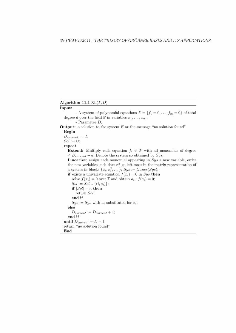
354CHAPTER 11. THE THEORY OF GROBNER BASES AND ITS APPLICATIONS
Algorithm 11.1 XL(F,D)
Input:- A system of polynomial equations F = f1 = 0, . . . , fm = 0 of total
degree d over the field F in variables x1, . . . , xn ;- Parameter D;
Output: a solution to the system F or the message “no solution found”BeginDcurrent := d;Sol := ∅;repeat
Extend: Multiply each equation fi ∈ F with all monomials of degree≤ Dcurrent − d; Denote the system so obtained by Sys;Linearize: assign each monomial appearing in Sys a new variable, orderthe new variables such that xai go left-most in the matrix representation ofa system in blocks xi, x2
i , . . . ; Sys := Gauss(Sys);if exists a univariate equation f(xi) = 0 in Sys then
solve f(xi) = 0 over F and obtain ai : f(ai) = 0;Sol := Sol ∪ (i, ai);if |Sol| = n then
return Sol;end ifSys := Sys with ai substituted for xi;
elseDcurrent := Dcurrent + 1;
end ifuntil Dcurrent = D + 1return “no solution found”End
11.1. POLYNOMIAL SYSTEM SOLVING 355
11.1.2 Grobner bases
In the previous section we saw how one can solve systems of non-linear equationsusing linearization techniques. Speaking the language of algebraic geometry, wewant to find elements of the variety V (f1, ..., fm), where V (f1, ..., fm) := a ∈Fn : ∀1 ≤ i ≤ m, fi(a) = 0 and F is a field. The target object of this section,Grobner basis technique, gives an opportunity to find this variety and also solvemany other important problems like for example ideal membership, i.e. decidingwhether a given polynomial may be obtained as a polynomial combination of thegiven set of polynomials. As we will see, the algorithm for finding Grobner basesgeneralizes Gaussian elimination for linear systems on one side and Euclideanalgorithm of finding the GCD of two univariate polynomials on the other side.We will see how this algorithm, the Buchberger’s algorithm, works and howGrobner bases can be applied for finding a variety (system solving) and someother problems. First of all, we need some definitions. *** should this go toAppendix? ***
Definition 11.1.4 Let R := F[x1, ...xn] be a polynomial ring in n variablesover the field F. An ideal in R is a subset of R with the following properties:
- 0 ∈ I;
- for every f, g ∈ I : f + g ∈ I;
- for every h ∈ R and every f ∈ I : h · f ∈ R.
So the ideal I is a subset of R closed under addition and closed under multi-plication with elements from R. Let f1, . . . , fm ∈ R. It is easy to see that theobject 〈f1, . . . , fm〉 := a1f1 + · · · + amfm|ai ∈ R ∀i is an ideal. We say that〈f1, . . . , fm〉 is an ideal generated by the polynomials f1, . . . , fm. From commu-tative algebra it is know that every ideal I has a finite system of generators, i.e.I = 〈f1, . . . , fm〉 for some f1, . . . , fm ∈ I. A Grobner basis, that we define later,is a system of generators with special properties.A monomial in R is a product of the form xa1
1 · · · · · xann with a1, . . . , an beingnon-negative integers. Denote X = x1, . . . , xn and by Mon(X) the set of allmonomials in R.
Definition 11.1.5 A monomial ordering on R is any relation > on Mon(X)such that
- > is a total ordering on Mon(X), i.e. any two elements of Mon(X) arecomparable;
- > is multiplicative, i.e. Xα > Xβ implies Xα · Xγ > Xβ · Xγ for allvectors γ with non-negative integer entries, here Xα = xα1
1 · · · · · xαnn ;
- > is a well-ordering, i.e. every non-empty subset ofMon(X) has a minimalelement.
Example 11.1.6 Here are some orderings that are frequently used in practice.
1. Lexicographic ordering induced by x1 > · · · > xn : Xα >lp Xβ if and only
if there exists an s such that α1 = β1, . . . , αs−1 = βs−1, αs > βs.
356CHAPTER 11. THE THEORY OF GROBNER BASES AND ITS APPLICATIONS
2. Degree reverse lexicographic ordering induced by x1 > · · · > xn : Xα >dpXβ if and only if |α| := α1+· · ·+αn > β1+· · ·+βn =: |β| or if |α| = |β| andthere exists an s such that αn = βn, . . . , αn−s+1 = βn−s+1, αn−s < βn−s.
3. Block ordering or product ordering. Let X and Y be two ordered sets ofvariables, >1 a monomial ordering on F[X] and >2 a monomial ordering onF[Y ]. The block ordering on F[X,Y ] is the following: Xα1Y β1 > Xα2Y β2
if and only if Xα1 >1 Xα2 or if Xα1 =1 X
α2 and Y β1 >2 Yβ2 .
Definition 11.1.7 Let > be a monomial ordering on R. Let f =∑α cαX
α bea non-zero polynomial from R. Let α0 be such that cα0
6= 0 and Xα0 > Xα forall α 6= α0 with cα 6= 0. Then lc(f) := cα0 is called the leading coefficient of f ,lm(f) := Xα0 is called the leading monomial of f , lt(f) := cα0X
α0 is called theleading term of f , moreover tail(f) := f − lt(f).
Having these notions we are ready to define the notion of a Grobner basis.
Definition 11.1.8 Let I be an ideal in R. The leading ideal of I with respectto > is defined as L>(I) := 〈lt(f)|f ∈ I, f 6= 0〉. The L>(I) is abbreviated byL(I) if it is clear which ordering is meant. A finite subset G = g1, . . . , gm of Iis called a Grobner basis for I with respect to > if L>(I) = 〈lt(g1), . . . , lt(gm)〉.We say that the set F = f1, . . . , fm is a Grobner basis if F is a Grobner basisof the ideal 〈F 〉.
Remark 11.1.9 Note that a Grobner basis of an ideal is not unique. The so-called reduced Grobner basis of an ideal is unique. By this one means a Grobnerbasis G in which all elements have leading coefficient equal to 1 and no leadingterm of an element g ∈ G divides any of the terms of g′, where g 6= g′ ∈ G.
Historically the first algorithm for computing Grobner bases was proposed byBruno Buchberger in 1965. In fact the very notion of the Grobner basis wasintroduced by Buchberger in his Ph.D. thesis and was named after his Ph.D.advisor Wolfgang Grobner. In order to be able to formulate the algorithm weneed two more definitions.
Definition 11.1.10 Let f, g ∈ R \ 0 be two non-zero polynomials, and letlm(f) and lm(g) be leading monomials of f and g resp. w.r.t some monomialordering. Denote m := lcm(lm(f), lm(g)). Then the s-polynomial of these twopolynomials is defined as
spoly(f, g) = m/lm(f) · f − lc(f)/lc(g) ·m/lm(g) · g.
Remark 11.1.11 1. If lm(f) = xa11 · . . . xann and lm(g) = xb11 · · · · · xbnn , then
m = xc11 · . . . xcnn , where ci = max(ai, bi) for all i. Therewith m/lm(f) andm/lm(g) are monomials.
2. Note that if we write f = lc(f) · lm(f) + f ′ and g = lc(g) · lm(g) + g′,where lm(f ′) < lm(f) and lm(g) < lm(g′), then spoly(f, g) = m/lm(f) ·(lc(f) · lm(f) + f ′)− lc(f)/lc(g) ·m/lm(g) · (lc(g) · lm(g) + g′) = m · lc(f) +m/lm(f) · f ′ − m · lc(f) − lc(f)/lc(g) · m/lm(g) · g′ = m/lm(f) · f ′ −lc(f)/lc(g) ·m/lm(g) · g′. Therewith we “canceled out” the leading termsof both f and g.
11.1. POLYNOMIAL SYSTEM SOLVING 357
Example 11.1.12 In order to understand this notion better, let us see whatare the s-polynomials in the case of linear and univariate polynomials
linear: Let R = Q[x, y, z] and a monomial ordering being lexicographic with x >y > z. Let f = 3x+2y−10z, g = x+5y−5z, then lm(f) = lm(g) = x,m =x : spoly(f, g) = f − 3/1 · g = 3x+ 2y− 10z− 3x− 15y+ 15z = −13y+ 5zand this is exactly what one would do to cancel out the variable x duringthe Gaussian elimination.
univariate: Let R = Q[x]. Let f = 2x5 − x3, g = x2 − 10x + 1, then m = x5 andspoly(f, g) = f − 2/1 · x3 · g = 2x5 − x3 − 2x5 + 20x4 − 2x3 = 20x4 − 3x3
and this is the first step in polynomial division algorithm, which is usedin the Euclidean algorithm for finding gcd(f, g).
To define the next notion we need for the Buchberger’s algorithm, we use thefollowing result.
Theorem 11.1.13 Let f1, . . . , fm ∈ R \ 0 be non-zero polynomials in thering R endowed with a monomial ordering < and let f ∈ R be some polynomial.Then there exist polynomials a1, . . . , am, h ∈ R with the following properties:
1. f = a1 · f1 + · · ·+ am · fm + h;
2. lm(f) ≥ lm(ai · fi) for f 6= 0 and every i such that ai · fi 6= 0;
3. if h 6= 0, then lm(h) is not divisible by any of lm(ai · fi).
Moreover,if G = f1, . . . , fm is a Grobner basis, then the polynomial h isunique.
Definition 11.1.14 Let F = f1, . . . , fm ⊂ R and f ∈ R. We define thenormal form of f w.r.t F to be any h from Theorem 11.1.13. Notation isNF(f |F ) := h.
Remark 11.1.15 1. If R = F[x] and f1 := g ∈ R, then NF (f |〈g〉) is exactlythe remainder of division of the univariate polynomial f by the polynomialg. So the notion of a normal form generalizes the notion of a remainderfor the case of a multivariate polynomial ring.
2. The notion of a normal form is uniquely defined only if f1, . . . , fm is aGrobner basis.
3. Normal form has a very important property: f ∈ I ⇐⇒ NF(f |G) = 0,where G is a Grobner basis of I. So by computing a Grobner basis of thegiven ideal I and then computing the normal form of the given polynomialf we may decide whether f belongs to I or not.
The algorithm for computing a normal form proceeds as in Algorithm 11.2.In Algorithm 11.2 the function Exists_LT_Divisor(F,h) returns an index isuch that lt(fi) divides lt(h) if such index exists and 0 otherwise. Note that thealgorithm may also be adapted so that it returns the polynomial combination offi’s such that together with h it satisfies conditions (1)–(3) of Theorem 11.1.13.
358CHAPTER 11. THE THEORY OF GROBNER BASES AND ITS APPLICATIONS
Algorithm 11.2 NF(f |F )
Input:- Polynomial ring R with monomial ordering <- Set of polynomials F = f1, . . . , fm ⊂ R- Polynomial f ∈ R
Output: a polynomial h which satisfies (1)–(3) of Theorem 11.1.13 for the setF and the polynomial f with some ai’s from RBeginh := f ;i :=Exists_LT_Divisor(F, h);while h 6= 0 and i doh := h− lt(h)/lt(fi) ∗ fi;i :=Exists_LT_Divisor(F, h);
end whilereturn hEnd
Example 11.1.16 Let R = Q[x, y] and the monomial ordering being lexico-graphic ordering with x > y. Let f = x2 − y3 and F = f1, f2 = x2 +x + y, x3 + xy + y3. At the beginning of Algorithm 11.2 h = f . NowExists_LT_Divisor(F,h)=1 so we enter the while-loop. In the while-loop fol-lowing assignment is made h := h−lt(h)/lt(f1)·f1 = x2−y3−x2/x2·(x2+x+y) =−x − y3 − y. We compute again Exists_LT_Divisor(F,h)=0. So we do notenter in the second loop and h = −x− y3 − y is a normal form of f we lookedfor.
Now we are ready to formulate the Buchberger’s algorithm for finding a Grobnerbasis of an ideal: Algorithm 11.3.The main idea of the algorithm is: if after “canceling” leading terms of thecurrent pair (also called a critical pair) we cannot “divide” the result by thecurrent set, then add the result to this set and add all new pairs to the set ofcritical pairs. The next example shows the algorithm in action.
Example 11.1.17 We take as a basis Example 11.1.16. So R = Q[x, y] withthe monomial ordering being lexicographic ordering with x > y, and we havef1 = x2 + x + y, f2 = x3 + xy + y3. Initialization phase yields G := f1, f2and Pairs := (f1, f2). Now we enter the while-loop. We have to computeh = NF(spoly(f1, f2)|G). First, spoly(f1, f2) = x · f1− f2 = x3 +x2 +xy−x3−xy−y3 = x2−y3. As we know from Example 11.1.16, NF(x2−y3|G) = −x−y3−yand is non-zero. Therefore, we add f3 := h to G and add pairs (f3, f1) and(f3, f2) to Pairs. Recall that pair (f1, f2) is no longer in Pairs, so now we havetwo elements there.In the second run of the loop we take the pair (f3, f1) and remove it fromPairs. Now spoly(f3, f1) = −xy3 − xy + x + y and NF(−xy3 − xy + x +y|G) = y6 + 2y4 − y3 + y2 =: f4. We update the sets G and Pairs. NowPairs = (f3, f2), (f4, f1), (f4, f2), (f4, f3) and G = f1, f2, f3, f4. Next takethe pair (f3, f2). For this pair spoly(f3, f2) = −x2y3 − x2y + xy + y3 andNF(spoly(f3, f2)|G) = 0. It may be shown that likewise all the other pairsfrom the set Pairs reduce to 0 w.r.t G. Therefore, the algorithm outputsG = f1, f2, f3, f4 as a Grobner basis of 〈f1, f2〉 w.r.t lexicographic ordering.
11.1. POLYNOMIAL SYSTEM SOLVING 359
Algorithm 11.3 Buchberger(F )
Input:- Polynomial ring R with monomial ordering <- Normal form procedure NF- Set of polynomials F = f1, . . . , fm ⊂ R
Output: Set of polynomials G ⊂ R such that G is a Grobner basis of the idealgenerated by the set F w.r.t monomial ordering <BeginG := f1, . . . , fm;while Pairs 6= empty doSelect a pair (f, g) ∈ Pairs;Remove the pair (f, g) from Pairs;h := NF(spoly(f, g)|G);if h 6= 0 then
for all p ∈ G doAdd pair (h, p) to Pairs;
end forAdd h to G;
end ifend whilereturn GEnd
Example 11.1.18 [CAS] Now we will show how to compute the above exam-ples in Singular and Magma. In Singular one has to execute the following code:> ring r=0,(x,y),lp;
> poly f1=x2+x+y;
> poly f2=x3+xy+y3;
> ideal I=f1,f2;
> ideal GBI=std(I);
> GBI;
GBI[1]=y6+2y4-y3+y2
GBI[2]=x+y3+y
One may request computation of the reduced Grobner basis by switching on theoption option(redSB). In the above example GBI is already reduced. Now ifwe compute the normal form of f1-f2 w.r.t GBI it should be zero.> NF(f1-f2,GBI);
0
It is also possible to track computations for small examples using LIB"teachstd.lib";.One should add this line at the beginning of the above piece of code togetherwith the line printlevel=1;, which makes program comments visible. Thenone should use standard(I) instead of std(I) to see the run in detail. Simi-larly, NFMora(f1-f2,I) should be used instead of NF(f1-f2,I).In Magma the following pieace of code does the job:> P<x,y> := PolynomialRing(Rationals(), 2, "lex");
> I:=[x^2+x+y,x^3+x*y+y^3];
> G:=GroebnerBabsis(I);
> NormalForm(I[1]-I[2],G);
360CHAPTER 11. THE THEORY OF GROBNER BASES AND ITS APPLICATIONS
Now that we have introduced techniques necessary to compute Grobner bases,let us demonstrate one of the main applications of Grobner bases, namely poly-nomial system solving. The following result shows how one can solve a poly-nomial system of equations, provided one can compute a Grobner basis w.r.tlexicographic ordering.
Theorem 11.1.19 Let f1(X) = · · · = fm(X) = 0 be a system of polynomialequations defined over F[X] with X = (x1, . . . , xn), such that it has finitelymany solutions 1. Let I = 〈f1, . . . , fm〉 be an ideal defined by the polynomialsin the system and let G be a Grobner basis for I with respect to >lp induced byxn < · · · < x1. Then there are elements g1, . . . , gn ∈ G such that
gn ∈ F[xn], lt(gn) = cnxmnn ,
gn−1 ∈ F[xn−1, xn], lt(gn−1) = cn−1xmn−1
n−1 ,. . .g1 ∈ F[x1, . . . , xn], lt(g1) = c1x
m11 .
for some positive integers mi, i = 1, . . . , n and elements ci ∈ F\0, i = 1, . . . , n.
It is clear how to solve the system I now. After computing G, first solve a
univariate equation gn(xn) = 0. Let a(n)1 , . . . , a
(n)ln
be the roots. For every
a(n)i then solve gn−1(xn−1, a
(n)i ) = 0 to find possible values for xn−1. Repeat
this process until all the coordinates of all candidate solutions are found. Thecandidates form a finite set Can ⊆ Fn. Test all other elements of G on whetherthey vanish at elements of Can. If there is some g ∈ G that does not vanish atsome can ∈ Can, then discard can from Can. Since the number of solutions isfinite the above procedure terminates.
Example 11.1.20 Let us be more specific and give a concrete example of howTheorem 11.1.19 can be applied. Turn back to Example 11.1.17. Suppose wewant to solve a system of equations x2 + x + y = 0, x3 + xy + y3 = 0 over therationals. We compute a Grobner basis of the corresponding ideal and obtainthat elements f4 = y6 +2y4−y3 +y2 and f3 = −x−y3−y belong to the Grobnerbasis. Since f4 has finitely many solutions (at most 6 over the rationals) and forevery fixed value of y f3 has exactly one solution of x, we actually know thatour system has finitely many solutions, both over the rationals and its algebraicclosure. In order to find solutions, we have to solve the univariate equationy6 +2y4−y3 +y2 = 0 for y. If we factorize, we obtain f4 = y2(y4 +2y2−y+1),where y4 + 2y2 − y + 1 is irreducible over Q. So from the equation f4 = 0 weonly get y = 0 as a solution. Then for y = 0 the equation f3 = 0 yields x = 0.Therefore, over rationals the given system has a unique solution (0, 0).
Example 11.1.21 Let us consider another example. Consider the following
1Rigorously speaking, we rewuire the system to have finitely many solutions in F. Suchsystems (ideals) are called zero-dimensional.
11.1. POLYNOMIAL SYSTEM SOLVING 361
system over F2:xy + x+ y + z = 0,xz + yz + y = 0,x+ yz + z = 0,x2 + x = 0,y2 + y = 0,z2 + z = 0.
Note that the field equations x2 + x = 0, y2 + y = 0, z2 + z = 0 make sure thatany solution for the first three equations actually lies in F2. Since F2 is a finitefield, we automatically get that the system above has finitely many solutions(in fact not more than 23 = 8). One can show that reduced Grbner basis (seeRemark 11.1.9) w.r.t lexicographic ordering with x > y > z of the correspondingideal is: G = z2 + z, y+ z, x. From this we obtain that the system in questionhas two solutions: (0, 0, 0) and (0, 1, 1).
In Sections 11.2 and 11.2 we will see many more situations when Grobner basesare applied in the solving context. Grobner basis techniques are also used foranswering many other important questions. To end this section, we give onesuch application. *** should this go to Section 11.3? ***
Example 11.1.22 Sometimes it is needed to obtain explicit equations relatingcertain variables from given implicit ones. The following example is quite typicalin algebraic cryptanalysis of block ciphers. One of the main building blocks ofmodern block ciphers are the so-called S–Boxes, local non-linear transformationsthat in composition with other, often linear, mappings compose a secure blockcipher. Suppose we have an S–Box S that transforms a 4-bit vector into a 4-bit vector in a non-linear way as follows. Consider a non-zero binary vector xas an element in F24 via an identification of F4
2 and F24 = F2[a]/〈a4 + a + 1〉done in a usual way, so that e.g. a vector (0, 1, 0, 0) is mapped to the primitiveelement a, and (0, 1, 0, 1) is mapped to a + a3. Now if x is considered as anelement of F24 the S–Box S maps it to y = x−1 and then considers it againas a vector via the above identification. The zero vector is mapped to the zerovector. Not going deeply into details, we just state that such a transformationcan be represented over F2 as a system of quadratic equations that implicitlyrelate the input variables x with the output variables y. The equations are
y0x0 + y3x1 + y2x2 + y1x3 + 1 = 0,y1x0 + y0x1 + y3x1 + y2x2 + y3x2 + y1x3 + y2x3 = 0,y2x0 + y1x1 + y0x2 + y3x2 + y2x3 + y3x3 = 0,y3x0 + y2x1 + y1x2 + y0x3 + y3x3 = 0,
together with the field equations x2i + xi = 0 and y2
i + yi = 0 for i = 0, . . . , 3.The equations do not describe the part when 0 is mapped to 0, so only theinversion is modeled.In certain situations it is more preferable to have explicit relations that wouldshould how the output variables y depend on the input variables x. For thisthe following technique is used. Consider the above equations as polynomialsin the same polynomial ring F2[y0, . . . , y3, x0, . . . , x3] with y0 > · · · > y3 > x0 >· · · > x3 w.r.t the block ordering with blocks being y- and x-variables, and theordering is degree reverse lexicographic in each block (see Example 11.1.6). In
362CHAPTER 11. THE THEORY OF GROBNER BASES AND ITS APPLICATIONS
this ordering, each monomial in y-variables will be larger than any monomialin x-variable, regardless of their degree. This ordering is a so-called eliminationordering for y variables. The reduced Grobner basis of the ideal composed ofthe above equations is
x2i + xi,
the field equations on x;
(x0 + 1) · (x1 + 1) · (x2 + 1) · (x3 + 1),
which provides that x should not be the all-zero vector, and
y3 + x1x2x3 + x0x3 + x1x3 + x2x3 + x1 + x2 + x3,y2 + x0x2x3 + x0x1 + x0x2 + x0x3 + x2 + x3,y1 + x0x1x3 + x0x1 + x0x2 + x1x2 + x1x3 + x3,y0 + x0x1x2 + x1x2x3 + x0x2 + x1x2 + x0 + x1 + x2 + x3,
which give explicit relations on y in terms of x. Interestingly enough, the fieldequations together with the latter explicit equations describe the entire S–Boxtransformation, so the case 0 7→ 0 is also covered.
Using similar techniques one may obtain other interesting properties of ideals,which come in hand in different applications.
11.1.3 Exercises
11.1.1 Let R = Q[x, y, z] and let F = f1, f2 with f1 = x2 + xy + z2, f2 =y2 + z and let f = x3 + 2y3 − z3. The monomial ordering is degree lexico-graphic. Compute NF(f |F ). Use the procedure NFMora from the Singular’steachstd.lib to check your result 2.
11.1.2 Let R = F2[x, y, z] and let F = f1, f2 with f1 = x2 + xy + z2, f2 =xy + z2. The monomial ordering is lexicographic. Compute a Grobner basis of〈F 〉. Use the procedure standard from the Singular’s teachstd.lib to checkyour result.
11.1.3 [CAS] Recall that in Example 11.1.20 we came to the conclusion thatthe only solution over the rationals for the system is (0, 0). Use Singular’s librarysolve.lib and in particular the command solve to find also complex solutionsof this system.
11.1.4 Upgrade Algorithm 11.2 so that it also returns ai’s from Theorem11.1.19.
11.1.5 Prove the so-called product criterion: if polynomials f and g are suchthat lm(f) and lm(g) are co-prime, then NF(spoly(f, g)|f, g) = 0.
11.1.6 Do the following sets constitute a Grobner basis:
2By setting printing level appropriately, procedures of teachstd.lib enable tracking theirrun. Therewith one may see exactly what a corresponding algorithm is doing.
11.2. DECODING CODES WITH GROBNER BASES 363
1. F1 := xy + 1, yz + x+ y + 2 ⊂ Q[x, y, z] with the degree ordering beingdegree lexicographic?
2. F2 := x+20, y+10, z+12, u+1 ⊂ F23[x, y, z, u] with the degree orderingbeing the block ordering with blocks (x, y) and (z, u) and degree reverselexicographic ordering inside the blocks?
11.2 Decoding codes with Grobner bases
As the first application of the Grobner basis method we consider decoding linearcodes. For the clarity of presentation we make an emphasis on cyclic codes. Weconsider Cooper’s philosophy or the power sums method in Section 11.2.1 andthe method of generalized Newton identities in Section 11.2.2. In Section 11.2.3we provide a brief overview of methods for decoding general linear codes.
11.2.1 Cooper’s philosophy
Now we will give an introduction to the so-called Cooper’s philosophy or thepower sums method. This method uses the special form of a parity-check matrixof a cyclic code. The main idea is to write these parity check equations withunknowns for error positions and error values and then solve with respect tothese unknowns by adding some natural restrictions on them.Let F = Fqm be the splitting field of Xn − 1 over Fq. Let a be a primitive n-throot of unity in F. If i is in the defining set of a cyclic code C (Definition ??),then
(1, ai, . . . , a(n−1)i)cT = c0 + c1ai + · · ·+ cn−1a
(n−1)i = c(ai) = 0,
for every codeword c ∈ C. Hence (1, ai, . . . , a(n−1)i) is a parity check of C. Leti1, . . . , ir be a defining set of C. Then a parity check matrix H of C can berepresented as a matrix with entries in F (see also Section 7.5.3):
H =
1 ai1 a2i1 . . . a(n−1)i1
1 ai2 a2i2 . . . a(n−1)i2
......
.... . .
...1 air a2ir . . . a(n−1)ir
.
Let c, r and e be the transmitted codeword, the received word and the errorvector, respectively. Then r = c + e. Denote the corresponding polynomials byc(x), r(x) and e(x), respectively. If we apply the parity check matrix to r, weobtain
sT := HrT = H(cT + eT ) = HcT +HeT = HeT ,
since HcT = 0, where s is the syndrome vector. Define si = r(ai) for alli = 1, . . . , n. Then si = e(ai) for all i in the complete defining set, and thesesi are called the known syndromes. The remaining si are called the unknownsyndromes. We have that the vector s above has entries s = (si1 , . . . , sir ). Let tbe the number of errors that occurred while transmitting c over a noisy channel.If the error vector is of weight t, then it is of the form
e = (0, . . . , 0, ej1 , 0, . . . , 0, ejl , 0, . . . , 0, ejt , 0, . . . , 0).
364CHAPTER 11. THE THEORY OF GROBNER BASES AND ITS APPLICATIONS
More precisely there are t indices jl with 1 ≤ j1 < · · · < jt ≤ n such that ejl 6= 0for all l = 1, . . . , t and ej = 0 for all j not in j1, . . . , jt. We obtain
siu = r(aiu) = e(aiu) =
t∑l=1
ejl(aiu)jl , 1 ≤ u ≤ r. (11.2)
The aj1 , . . . , ajt but also the j1, . . . , jt are the error locations, and the ej1 , . . . , ejtare the error values. Define zl = ajl and yl = ejl . Then z1, . . . , zt are the errorlocations and y1, . . . , yt are the error values and the syndromes in (11.2) becomegeneralized power sum functions
siu =
t∑l=1
ylziul , 1 ≤ u ≤ r. (11.3)
In the binary case the error values are yi = 1, and the syndromes are the ordi-nary power sums.
Now we give a description of Cooper’s philosophy. As the receiver does not knowhow many errors occurred, the upper bound t is replaced by the error-correctingcapacity e and some zl’s are allowed to be zero, while assuming that the numberof errors is at most the error-correcting capacity e. The following variables areintroduced: X1, . . . , Xr, Z1, . . . , Ze and Y1, . . . , Ye, where Xu stands for thesyndrome siu , 1 ≤ u ≤ r; Zl stands for the error location zl for 1 ≤ l ≤ t, and 0for t < l ≤ e; and finally Yl stands for the error value yl for 1 ≤ l ≤ t, and anyelement of Fq \ 0 for t < l ≤ e. The syndrome equations (11.2) are rewrittenin terms of these variables as power sums:
fu :=
e∑l=1
YlZiul −Xu = 0, 1 ≤ u ≤ r.
We also add some other equations in order to specify the range of values thatcan be achieved by our variables, namely:
εu := Xqm
u −Xu = 0, 1 ≤ u ≤ r,
since sj ∈ F; *** add field equations in the Appendix ***
ηl := Zn+1l − Zl = 0, 1 ≤ l ≤ e,
since ajl are either n-th roots of unity or zero; and
λl := Y q−1l − 1 = 0, 1 ≤ l ≤ e,
since yl ∈ Fq \ 0. We obtain the following set of polynomials in the variablesX = (X1, . . . , Xr), Z = (Z1, . . . , Ze) and Y = (Y1, . . . , Ye):
FC = fu, εu, ηl, λl : 1 ≤ u ≤ r, 1 ≤ l ≤ e ⊂ Fq[X,Z, Y ]. (11.4)
The zero-dimensional ideal IC generated by FC is called the CRHT-syndromeideal associated to the code C, and the variety V (FC) defined by FC is calledthe CRHT-syndrome variety, after Chen, Reed, Helleseth and Truong. We have
11.2. DECODING CODES WITH GROBNER BASES 365
V (FC) = V (IC).
Initially decoding of cyclic codes was essentially brought to finding the re-duced Grobner basis of the CRHT-ideal. Unfortunately, the CRHT-varietyhas many spurious elements, i.e. elements that do not correspond to error po-sitions/values. It turns out that adding more polynomials to the CRHT-idealgives an opportunity to eliminate these spurious elements. By adding polyno-mials
χl,m := ZlZmp(n,Zl, Zm) = 0, 1 ≤ l < m ≤ e
to FC , where
p(n,X, Y ) =Xn − Y n
X − Y=
n−1∑i=0
XiY n−1−i, (11.5)
we ensure that for all l and m either Zl and Zm are distinct or at least one ofthem is zero. The resulting set of polynomials is
F ′C := fu, εu, ηi, λi, χl,m : 1 ≤ u ≤ r, 1 ≤ i ≤ e, 1 ≤ l < m ≤ e ⊂ Fq[X,Z, Y ].(11.6)
The ideal generated by F ′C is denoted by I ′C . By investigating the structure ofI ′C and its reduced Grobner basis with respect to lexicographic order inducedby X1 < · · · < Xr < Ze < · · · < Z1 < Y1 < · · · < Ye, the following result maybe proven.
Theorem 11.2.1 Every cyclic code C possesses a general error-locator polyno-mial LC . This means that there exists a unique polynomial LC ∈ Fq[X1, . . . , Xr, Z]that satisfies the following two properties:
• LC = Ze + at−1Ze−1 + · · ·+ a0 with aj ∈ Fq[X1, . . . , Xr], 0 ≤ j ≤ e− 1;
• given a syndrome s = (si1 , . . . , sir ) ∈ Fr corresponding to an error ofweight t ≤ e and error locations k1, . . . , kt, if we evaluate the Xu = siufor all 1 ≤ u ≤ r, then the roots of LC(s, Z) are exactly ak1 , . . . , akt and0 of multiplicity e− t, in other words
LC(s, Z) = Ze−tt∏i=1
(Z − aki).
Moreover, LC belongs to the reduced Grobner basis of the ideal I ′C and its is aunique element, which is a univariate polynomial in Ze of degree e. *** checkthis ***
Having this polynomial, decoding of the cyclic code C reduces to univariatefactorization. The main effort here is finding the reduced Grobner basis of I ′C .In general this is infeasible already for moderate size codes. For small codes,though, it is possible to apply this technique successfully.
Example 11.2.2 As an example we consider finding the general error locatorpolynomial for a binary cyclic BCH code C with parameters [15,7,5] that corrects2 errors. This code has 1, 3 as a defining set. So here q = 2,m = 4, and n = 15.The field F16 is the splitting field of X15 − 1 over F2. In the above descriptionwe have to write equations for all syndromes that correspond to elements in
366CHAPTER 11. THE THEORY OF GROBNER BASES AND ITS APPLICATIONS
the complete defining set. Note that we may write the equations only for theelements from the defining set 1, 3 as all the others are just consequences ofthose. Following the description above we write generators F ′C of the ideal I ′Cin the ring F2[X1, X2, Z1, Z2]:
Z1 + Z2 −X1, Z31 + Z3
2 −X2,X16
1 −X1, X162 −X2,
Z161 − Z1, Z16
2 − Z2,Z1Z2p(15, Z1, Z2).
We suppress the equations λ1 and λ2 as error values are over F2. In orderto find the general error locator polynomial we compute the reduced Grobnerbasis G of the ideal I ′C with respect to the lexicographical order induced byX1 < X2 < Z2 < Z1. The elements of G are:
X161 +X1,
X2X151 +X2,
X82 +X4
2X121 +X2
2X31 +X2X
61 ,
Z2X151 + Z2,
Z22 + Z2X1 +X2X
141 +X2
1 ,Z1 + Z2 +X1
According to Theorem 11.2.1 the general error correcting polynomial LC is aunique element of G of degree 2 with respect to Z2. So LC ∈ F2[X1, X2, Z] is
LC(X1, X2, Z) = Z2 + ZX1 +X2X141 +X2
1 .
Let us see how decoding using LC works. Let
r = (1, 1, 0, 1, 0, 0, 0, 0, 0, 0, 1, 1, 1, 0, 1)
be a received word with 2 errors. In the field F16 with a primitive element a,such that a4 + a + 1 = 0, a is also a 15-th root of unity. Then the syndromesare s1 = a2, s3 = a14. Plug them into LC in place of X1 and X2 and obtain:
LC(Z) = Z2 + a2Z + a6.
Factorizing yields LC = (Z + a)(Z + a5). According to Theorem 11.2.1, expo-nents 1 and 5 show exactly the error locations minus 1. So that errors occurredon positions 2 and 6.
Example 11.2.3 [CAS] All the computations in the previous example may beundertaken using the library decodegb.lib of Singular. The following Singular-code yields the CRHT-ideal and its reduced Grobner basis.> LIB "decodegb.lib";
> // binary cyclic [15,7,5] code with a defining set (1,3)
> list defset=1,3; // defining set
> int n=15; // length
> int e=2; // error-correcting capacity
> int q=2; // base field size
> int m=4; // degree extension of the splitting field
> int sala=1; // indicator to add additional equations as in (11.5)
11.2. DECODING CODES WITH GROBNER BASES 367
> def A=sysCRHT(n,defset,e,q,m,sala);
> setring A; // set the polynomial ring for the system ’crht’
> option(redSB); // compute reduced Groebner basis
> ideal red_crht=std(crht);
Now, inspecting the ideal red_crht we see which polynomial should we take asa general error-locator polynomial according to Theorem 11.2.1.> poly gen_err_loc_poly=red_crht[5];
At this point we have to change to a splitting field in order to do our furthercomputations.> list l=ringlist(basering);
> l[1][4]=ideal(a4+a+1);
> def B=ring(l);
> setring B;
> poly gen_err_loc_poly=imap(A,gen_err_loc_poly);
We can now process our received vector and compute the syndromes:> matrix rec[1][n]=1,1,0,1,0,0,0,0,0,0,1,1,1,0,1;
> matrix checkrow1[1][n];
> matrix checkrow3[1][n];
> int i;
> number work=a;
> for (i=0; i<=n-1; i++)
> checkrow1[1,i+1]=work^i;
>
> work=a^3;
> for (i=0; i<=n-1; i++)
> checkrow3[1,i+1]=work^i;
>
> // compute syndromes
> matrix s1mat=checkrow1*transpose(rec);
> matrix s3mat=checkrow3*transpose(rec);
> number s1=number(s1mat[1,1]);
> number s3=number(s3mat[1,1]);
One can now substitute and solve> poly specialized_gen=substitute(gen_err_loc_poly,X(1),s1,X(2),s3);
> factorize(specialized_gen);
[1]:
_[1]=1
_[2]=Z(2)+(a)
_[3]=Z(2)+(a^2+a)
[2]:
1,1,1
One can also check that a^5=a^2+a.
So we have seen that it is theoretically possible to encode all the informationneeded for decoding a cyclic code in one polynomial. Finding this polynomial,though, is a quite challenging task. Moreover, note that the polynomial coef-ficients aj ∈ Fq[X1, . . . , Xr] may be quite dense, so it may be a problem evenjust to store the polynomial LC . The method, nevertheless, provides efficientclosed formulas for small codes that are relevant in practice. This method canbe adapted to correct erasures and to find the minimum distance of a code.
368CHAPTER 11. THE THEORY OF GROBNER BASES AND ITS APPLICATIONS
More information on these issues is in Notes.
11.2.2 Newton identities based method
In Section 7.5.2 and Section 7.5.3 we have seen how Newton identities can beused for efficient decoding of cyclic codes up to half the BCH bound. Now wewant to generalize this method and be able to decode up to half the minimumdistance. In order to correct more errors we have to pay a price. Systems wehave to solve are no longer linear, but quadratic. This is exactly where Grobnerbasis techniques come into play.Let us recall necessary notions. Note that we change the notation a bit, as it willbe convenient for the generalization. The error-locator polynomial is defined by
σ(Z) =
t∏l=1
(Z − zl).
If this product is expanded
σ(Z) = Zt + σ1Zt−1 + · · ·+ σt−1Z + σt,
then the coefficients σi are the elementary symmetric functions in the errorlocations z1, . . . , zt.
σi = (−1)i∑
1≤j1<j2<···<ji≤t
zj1zj2 . . . zji , 1 ≤ i ≤ t.
The syndromes si and the coefficients σi satisfy the following generalized Newtonidentities, see Proposition 7.5.8:
si +
t∑j=1
σjsi−j = 0, for all i ∈ Zn. (11.7)
Now suppose that the complete defining set of the cyclic code contains the 2tconsecutive elements b, . . . , b+ 2t− 1 for some b. Then d ≥ 2t+ 1 by the BCHbound. Furthermore the set of equations (11.7) for i = b + t, . . . , b + 2t − 1is a system of t linear equations in the unknowns σ1, . . . , σt with the knownsyndromes sb, . . . , sb+2t−1 as coefficients. Gaussian elimination solves the systemof equations with complexity O(t3). In this way we obtain the APGZ decodingalgorithm, see Section 7.5.3. See Example 7.5.11 for the algorithm in action ona small example.One may go further and obtain closed formulas or solve the decoding problemvia the key equation, see Section ?? Section ??. All the above mentioned algo-rithms from Chapter 7 decode up to the BCH error-correcting capacity, whichis often strictly smaller than the true capacity. A general method was out-lined by Berlekamp, Tzeng, Hartmann, Chien, and Stevens, where the unknownsyndromes were treated as variables. We have
si+n = si, for all i ∈ Zn,
since si+n = r(ai+n) = r(ai). Furthermore
sqi = (e(ai))q = e(aiq) = sqi, for all i ∈ Zn,
11.2. DECODING CODES WITH GROBNER BASES 369
and
σqm
i = σi, for all 1 ≤ i ≤ t.
So the zeros of the following set of polynomialsNewtont in the variables S1, . . . , Snand σ1, . . . , σt are considered.
Newtont
σq
m
i − σi, for all 1 ≤ i ≤ t,Si+n − Si, for all i ∈ Zn,Sqi − Sqi, for all i ∈ Zn,Si +
∑tj=1 σjSi−j , for all i ∈ Zn.
(11.8)
Solutions of Newtont are called generic, formal or one-step. Computing thesesolutions is considered as a preprocessing phase which has to be performed onlyone time. For the actual decoder for every received word r the variables Si arespecialized to the actual value si(r) for i ∈ SC . Alternatively one can solveNewtont together with the polynomials Si − si(r) for i ∈ SC . This is calledonline decoding. Note that obtaining general error-locator polynomial as in theprevious subsection is an example of formal decoding: this polynomial has tobe found only once.
Example 11.2.4 Let us consider an example of decoding using Newton identi-ties and such that the APGZ algorithm is not applicable. We consider a 3-errorcorrecting cyclic code of length 31 with a defining set 1, 5, 7. Note that BCHerror-correcting capacity of this code is 2. We are aiming now at correcting 3errors. Let us write the corresponding ideal:
σ1S31 + σ2S30 + σ3S29 + S1,σ1S1 + σ2S31 + σ3S30 + S2,σ1S2 + σ2S1 + σ3S31 + S3,σ1Si−1 + σ2Si−2 + σ3Si−3 + Si, 4 ≤ i ≤ 31,σ32i + σi, i = 1, 2, 3,Si+31 + Si, for all i ∈ Z31,S2i + S2i, for all i ∈ Z31,
Note that the equations Si+31 = Si, and S2i = S2i imply,
S21 + S2, S4
1 + S4, S81 + S8, S16
1 + S16,S2
3 + S6, S43 + S12, S8
3 + S24, S163 + S17,
S25 + S10, S4
5 + S20, S85 + S9, S16
5 + S18,S2
7 + S14, S47 + S28, S8
7 + S25, S167 + S19,
S23 + S6, S4
3 + S12, S83 + S24, S16
3 + S17,S2
11 + S22, S411 + S13, S8
11 + S26, S1611 + S21,
S215 + S30, S4
15 + S29, S815 + S27, S16
15 + S23,S2
31 + S31.
Our intent is to write σ1, σ2, σ3 in terms of known syndromes S1, S5, S7. Thenext step would be to compute the reduced Grobner basis of this system withrespect to some elimination order induced by S31 > · · · > S8 > S6 > S4 > · · · >S2 > σ1 > σ2 > σ3 > S7 > S5 > S1. Unfortunately the computation is quitetime consuming and the result is too huge to illustrate the idea. Rather, we
370CHAPTER 11. THE THEORY OF GROBNER BASES AND ITS APPLICATIONS
do online decoding, i.e. for a concrete received r compute syndromes S1, S5, S7,plug the values into the system and then find σ’s. Let
r = (0, 0, 1, 0, 0, 1, 1, 1, 1, 0, 1, 1, 0, 0, 1, 1, 0, 1, 0, 0, 0, 0, 0, 1, 0, 0, 1, 1, 0, 0, 1)
be a received word with three errors. So the known syndromes we need ares1 = a7, s5 = a25 and s7 = a29. Substitute these values into the system aboveand compute the reduced Grobner basis of the system. The reduced Grobnerbasis with respect to the degree reverse lexicographic order (here it is possibleto go without an elimination order, see Remark ??) restricted to the variablesσ1, σ2, σ3 is σ3 + a5,
σ2 + a3,σ1 + a7
Corresponding values for σ’s gives rise to the error locator polynomial:
σ(Z) = Z3 + a7Z2 + a3Z + a5.
Factoring this polynomial yields three roots: a4, a10, a22, which indicate errorpositions 5, 11, and 23.Note also that we could have worked only with the equations for S1, S5, S7, S3, S11, S15, S31,but the Grobner basis computation is harder then.
Example 11.2.5 [CAS] The following program fulfils the above computationusing decodegb.lib from Singular.> LIB"decodegb.lib";
> int n=31; // length
> list defset=1,5,7; // defining set
> int t=3; // number of errors
> int q=2; // base field size
> int m=5; // degree extension of the splitting field
> def A=sysNewton(n,defset,t,q,m);
> setring A;
> // change the ring to work in the splitting field
> list l=ringlist(basering);
> l[1][4]=ideal(a5+a2+1);
> def B=ring(l);
> setring B;
> ideal newton=imap(A,newton);
> matrix rec[1][n]=0,0,1,0,0,1,1,1,1,0,1,1,0,0,1,1,0,1,0,0,0,0,0,1,0,0,1,1,0,0,1;
> // compute the parity-check rows for defining set (1,5,7)
> // similarly to the example with CRHT
> ...
> // compute syndromes s1,s5,s7
> // analogously to the CRHT-example
> ...
> // substitute the known syndromes in the system
> ideal specialize_newton;
> for (i=1; i<=size(newton); i++)
> specialize_newton[i]=substitute(newton[i],S(1),s1,S(5),s5,S(7),s7);
>
11.2. DECODING CODES WITH GROBNER BASES 371
> option(redSB);
> // find sigmas
> ideal red_spec_newt=std(specialize_newton);
> // identify values of sigma_1m sigma_2, and sigma_3
> // find the roots of the error-locator
> ring solve=(2,a),Z,lp;minpoly=a5+a2+1;
> poly error_loc=Z3+(a4+a2)*Z2+(a^3)*Z+(a^2+1); // sigma’s plugged in
> factorize(error_loc);
So as we see, by using Grobner basis it is possible to go beyond the BCH error-correcting capacity. The price paid is the complexity of solving quadratic, asopposed to linear, systems. *** more stuff in notes ***
11.2.3 Decoding arbitrary linear codes
Now we will outline a couple of ideas that may be used for decoding arbitrarylinear codes up to the full error-correcting capacity.
Decoding affine variety codes with Fitzgerald-Lax
The following method generalizes ideas of Cooper’s philosophy to arbitrary lin-ear codes. In this approach the main notion is the affine variety code. LetP1, . . . , Pn be points in Fsq. It is possible to compute a Grobner basis of an idealI ⊆ Fq[U1, . . . , Us] of polynomials that vanish exactly at these points. DefineIq := I + 〈Xq
1 − X1, . . . , Xqs − Xs〉. So Iq is a 0-dimensional ideal. We have
V (Iq) = P1, . . . , Pn. An affine variety code C(I, L) = φ(L) is an image of theevaluation map
φ : R→ Fnq ,f 7→ (f(P1), . . . , f(Pn)),
where R := Fq[U1, . . . , Us]/Iq, L is a vector subspace of R and f is the cosetof f in Fq[U1, . . . , Us] modulo Iq. It is possible to show that every q-ary linear[n, k] code, or equivalently its dual, can be represented as an affine variety codefor certain choice of parameters. See Exercise 11.2.2 for such a construction inthe case of cyclic codes.In order to write a system of polynomial equations similar to the one in Sec-tion 11.2.1 one needs to generalize the CRHT approach to affine codes. Simi-larly to the CRHT method the system of equations (or equivalently the ideal)is composed of the “parity-check” part and the “constraints” part. Parity-check part is constructed according to the evaluation map φ. Now, as canbe seen from Exercise 11.2.2, the points P1, . . . , Pn encode positions in a vec-tor, similarly to how ai encode positions in the case of a cyclic code, a be-ing a primitive n-th root of unity. Therefore, one needs to add polynomials(gl(Xk1, . . . , Xks))l=1,...,m;k=1,...,t for every error position. Adding other naturalconstraints, like field equations on error values, and then computing a Grobnerbasis of the combined ideal IC w.r.t certain elimination ordering, it is possibleto recover both error positions (i.e. values of “error points”) and error values.In general, finding I and L is quite technical and it turns out that for randomcodes this method is quite poor, because of the complicated structure of IC .The method may be quite efficient, though, if a code has more structure, like inthe case of geometric codes (e.g. Hermitian codes). We mention also that there
372CHAPTER 11. THE THEORY OF GROBNER BASES AND ITS APPLICATIONS
are improvements of the approach of Fitzgerald and Lax, which follow the sameidea as the improvements for the CRHT-method. Namely, one adds polynomialsthat ensure that the error locations are different. It can be proven that affinevariety codes possess the so-called multi-dimensional general error-locator poly-nomial, which is a generalization of the general error-locator polynomial fromTheorem 11.2.1.
Decoding by embedding in an MDS code
Now we briefly outline a method that provides a system for decoding that iscomposed of at most quadratic equations. The main feature of the method isthat we do not need field equations for the solution to lie in a correct domain.Let C be an Fq-linear [n, k] code with error correcting capacity e. Choose aparity check matrix H of C. Let h1, . . . ,hr be the rows of H. Let b1, . . . ,bnbe a basis of Fnq . Let Bs be the s × n matrix with b1, . . . ,bs as rows, thenB = Bn. We say that b1, . . . ,bn is an ordered MDS basis and B an MDSmatrix if all the s × s submatrices of Bs have rank s for all s = 1, . . . , n. Notethat an MDS basis for Fnq always exists if n ≤ q. By extending an initial fieldto a sufficiently large degree, we may assume that an MDS basis exists there.Since the parameters of a code do not change when going to a scalar extension,we may assume that our code C is defined over this sufficiently large Fq withq ≥ n. Each row hi is then a linear combination of the basis b1, . . . ,bn, thatis there are constants aij ∈ Fq such that hi =
∑nj=1 aijbj . In other words
H = AB where A is the r×n matrix with entries aij . For every i and j, bi ∗bjis a linear combination of the basis vectors b1, . . . ,bn, so there are constantsµijl ∈ Fq such that bi ∗ bj =
∑nl=1 µ
ijl bl. The elements µijl ∈ Fq are called the
structure constants of the basis b1, . . . ,bn. Linear functions Uij in the variables
U1, . . . , Un are defined as Uij =∑nl=1 µ
ijl Ul.
Definition 11.2.6 For the received vector r the ideal J(r) in the ring Fq[U1, . . . , Un]is generated by the elements∑n
l=1 ajlUl − sj(r) for j = 1, . . . , r,
where s(r) is the syndrome of r. The ideal I(t,U , V ) in the ring Fq[U1, . . . , Un, V1, . . . , Vt]is generated by the elements∑t
j=1 UijVj − Ui,t+1 for i = 1, . . . , n.
Let J(t, r) be the ideal in Fq[U1, . . . , Un, V1, . . . , Vt] generated by J(r) andI(t,U , V ).
Now we are ready to state the main result of the method.
Theorem 11.2.7 Let B be an MDS matrix with structure constants µijl andlinear functions Uij. Let H be a parity check matrix of the code C such thatH = AB as above. Let r = c + e be a received word with c in C the codewordsent and e the error vector. Suppose that the weight of e is not zero and at moste. Let t be the smallest positive integer such that J(t, r) has a solution (u,v)over Fq. Then wt(e) = t and the solution is unique satisfying u = Be. Theerror vector is recovered as e = B−1u.
11.2. DECODING CODES WITH GROBNER BASES 373
So as we see, although we did not impose any field equations neither on U− noron V−variables, we still are able to obtain a correct solution. For the case ofcyclic codes by going to a certain field extension Fq it may be shown that thesystem I(t,U , V ) actually defines the generalized Newton identities. Thereforeone of the corollaries of the above theorem that it is actually possible to workwithout the field equations in the method of Newton identities.
Decoding by normal form computations
Another method for arbitrary linear codes has a different approach to howone represents code-related information. Below we outline the idea for binarycodes. Let [X] be a commutative monoid generated by X = X1, . . . , Xn. Thefollowing mapping associates a vector of reduced exponents to a monomial:
ψ : [X]→ Fn2 ,∏ni=1X
aii 7→ (a1 mod 2, . . . , an mod 2).
Now, let w1, . . . ,wk be rows of a generator matrix G of the binary [n, k] codeC with the error-correcting capacity e. Consider an ideal IC ⊆ K[X1, . . . , Xn],where K is an arbitrary field: I := 〈Xw1 − 1, . . . , Xwk − 1, X2
1 − 1, . . . , X2n− 1〉.
So the ideal IC encodes the information about the code C. The next theoremshows how one decodes using IC .
Theorem 11.2.8 Let GB be the reduced Grobner basis of IC w.r.t some degreecompatible monomial ordering <. If wt(ψ(NF (Xa, GB))) ≤ e, then ψ(NF (Xa, GB))is the error vector corresponding to the received word ψ(Xa), i.e. ψ(Xa) −ψ(NF (Xa, GB)) is the codeword of C, closest to ψ(Xa).
Note that IC is a binomial ideal, and therefore GB is also a binomial ideal.For binomial ideals a normal form of a monomial is again a monomial. So thecomputation in the theorem above are well-defined. Using the special structureof IC it is possible to improve on Grobner basis computations to obtain GB,compared to usual techniques.It is remarkable that the code-related information as well as a solution to thedecoding problem is represented by exponents of monomials, whereas in allthe methods we considered before these data are encoded as values of certainvariables.
11.2.4 Exercises
11.2.1 [CAS] Consider a binary cyclic code of length 21 with a defining set(1, 3, 7, 9). This code has parameters [21, 7, 8], see Example 7.4.8 and Example7.4.17. The BCH bound is 5, so we cannot correct more than 2 errors with themethods from Chapter 7. Use the full error-correction capacity and correct 3errors in some random codeword using methods from Section 11.2.1, Section11.2.2, and decodegb.lib from Singular. Note that finding the general error-locator polynomial is very intense, therefore use online decoding in the CRHT-method: plug in concrete values of syndromes before computing a Grobnerbasis.
11.2.2 Show how a cyclic code may be considered as an affine variety codefrom Section 11.2.3.
374CHAPTER 11. THE THEORY OF GROBNER BASES AND ITS APPLICATIONS
11.2.3 Using a method of normal forms decode one error in a random codewordof the Hamming code (Example 2.2.14). Try different coefficient fields, as wellas different monomial orderings. Do you always get the same result?
11.3 Algebraic cryptanalysis
In the previous section we have seen how polynomial system solving (via Grobnerbases) is used in the problem of decoding linear codes. In this section we brieflyhighlight another interesting application of polynomial system solving. Namely,we will be talking about algebraic cryptanalysis of block ciphers. Block ci-phers were introduced in Chapter 10 as one of the main tools for providingsecure symmetric communication. There we also mentioned that there existmethods for cryptanalyzing block ciphers, i.e. distinguishing them from randompermutations and using this for recovering secret key used for the encryption.Traditional methods of cryptanalysis are statistical in nature. A cryptanalystor attacker queries a cipher seen as a black-box and set up with an unknownkey with (possibly chosen) plaintexts and receives corresponding ciphertexts.By collecting many such pairs a cryptanalyst hopes to find statistical patternsthat would distinguish the cipher in question from a random permutation. Al-gebraic cryptanalysis takes another approach. In this approach a cryptanalystwrites down a system of polynomial equations over a finite field (usually F2),which corresponds to the cipher in question via modeling operations done bythe cipher during the encryption process (and also key schedule) as algebraic(polynomial) equations. Therewith the obtained system of equations reflectsthe encryption process; plaintext and ciphertext are parameters of the system;key is the unknown variable represented e.g. by bit variables. After pluggingin actual plaintext/ciphertext the system should yield the unknown secret keyas a solution. In theory, provided that plaintext- and key lengths coincide, anattacker needs only one pair of plaintext/ciphertext to recover the key3. Thisfeature distinguishes algebraic approach from the statistical one, where an at-tacker usually needs many pairs to observe some statistical pattern.We proceed as follows. In Section 11.3.1 we describe a toy cipher, which willthen be used to illustrate the idea outlined above. We will see how to writeequations for the toy cipher in Section 11.3.2. We will also see that it may bepossible to write equations in different ways, which can be important for actualsolving. In Section 11.3.3 we address the question of writing equations for anarbitrary S-Box.
11.3.1 Toy example
As a toy block cipher we will take an iterative (Definition 10.1.9) block cipher(Definition 10.1.3) with text/key length of 16 bits and a two-round encryption.Our toy cipher is an SP-network (Definition 10.1.12). Namely in every roundwe have a layer of local substitutions (S-Boxes) followed by a permutation layer.Specifically, the encryption algorithm proceeds as in Algorithm 11.4.In this Algorithm SBox inherits the main idea of the S-Box in the AES, seeSection 10.1.4. Namely, we divide the state vector w := (w0, . . . , w15) into fourblocks of 4 consecutive bits. Then each block of four bits is considered as an
3He/she may need a few pairs in case the size of a plaintext and key do not coincide
11.3. ALGEBRAIC CRYPTANALYSIS 375
element of the field F16∼= F2[x]/〈x4 + x+ 1〉. The SBox then takes this number
and outputs an inverse in F16 for non-zero inputs, or 0 ∈ F16 otherwise. Theso obtained number is then interpreted again as a vector over F2 of length 4.Now the permutation layer represented by Perm acts on the entire 16-bit statevector. The bit at position i, 0 ≤ i ≤ 15 is moved to position Pos(i), where
Pos(i) =
4 · i mod 15, 0 ≤ i ≤ 14,15, i = 15.
(11.9)
So Perm(w) = (wPos(1), . . . , wPos(15)). Interestingly enough, this permutationprovides optimal diffusion in a sense that full dependency is achieved alreadyafter 2 rounds, see Exercise 11.3.1.Schematically the encryption process of our toy cipher is depicted on Figure .... *** add figure ***
Algorithm 11.4 Toy cipher encryption
Input: A 16-bit plaintext p and a 16-bit key k.Output: A 16-bit ciphertext c.
BeginPerform initial key addition: w := p⊕ k =AddKey(p, k).for i = 1, . . . , 2 do
Perform S-box substitution: w :=SBox(w).Perform a permutation w :=Perm(w).Add the key: w :=AddKey(w, k) = w ⊕ k.
end forThe ciphertext is c := w.return cEnd
11.3.2 Writing down equations
Now let us turn to the question of how to write a system of equations thatdescribes the encryption algorithm as in Algorithm 11.4. We would like towrite equations on the bit level, i.e. over F2. Denote by p = (p0, . . . , p15) andc = (c0, . . . , c15) the plaintext and ciphertext variables that appear as param-eters in our system. Then k = (k0, . . . , k15) are unknown key variables. Letxi = (xi,0, . . . , xi,15), i = 0, 1 be the variables representing result of bitwise keyaddition, yi = (yi,0, . . . , yi,15), i = 1, 2 be variables representing outcome of theS-Boxes, and zi = (zi,0, . . . , zi,15), i = 1, 2 be results of the permutation layer.Now we can write the encryption process as the following system:
x0 = p+ k,
yi = SBox(xi−1), i = 1, 2,
zi = Perm(yi), i = 1, 2,
x1 = z1 + k,
c = z2 + k. (11.10)
Here SBox and Perm are some polynomial functions that act on variable-vectors according to Algorithm 11.4.
376CHAPTER 11. THE THEORY OF GROBNER BASES AND ITS APPLICATIONS
There are three operations that are performed in the algorithm: bitwise keyaddition, substitution via four 4-bit S-Boxes, and the permutation. The keyaddition is represented trivially as above and one can write it on the bit levelas, e.g. in the initial key addition: x0,j = pj + kj , 0 ≤ j ≤ 15. The permutationPerm also does not pose any problem. According to (11.9) we have that theblocks zi = Perm(yi), i = 1, 2 above are written as
zi,j = yi,Pos−1(j), 0 ≤ j ≤ 15,
where Pos−1(j) may be easily computed and in fact in this case we havePos−1 = Pos.An interesting question is how to write equations over F2 that would describe theS-Box transformation SBox. Since SBox is composed of four parallel S-Boxesthat perform inversion in F16, we may concentrate on writing equation for oneS-Box. Let a = (a0, a1, a2, a3) be input bits of the S-Box and b = (b0, b1, b2, b3)are the output bits. The way we defined S-Box, we should consider a 6= 0 asan element of F16 and then compute b = a−1 in F16. Afterwards we regard bas a vector in F4
2. The all-zero vector is mapped to the all-zero vector. Thedescribing equation for inversion over F16 for the case a 6= 0 is obviously simplya · b = 1 or, incorporating the case a = 0, b = a14. Let us concentrate on thecase a 6= 0. We would like to rewrite the equation a · b = 1 over F16 into asystem of equations over F2 which involves the bit variables ai’s and bj ’s. InExample 11.1.22 we have seen what these equations are. But how can we ob-tain those? Using the identification F16
∼= F2[x]/〈x4 +x+ 1〉 we identify vectors(a0, a1, a2, a3) and (b0, b1, b2, b3) from F4
2 with a = a0 + a1x + a2x2 + a3x
3 andb = b0 + b1x+ b2x
2 + b3x3. Now having the rule x4 +x+ 1 = 0 in mind we have
to perform the multiplication a · b and collect the coefficients for the exponentsof x. We have (considering that x4 = x+ 1, x5 = x2 + x, x6 = x3 + x2):
a · b = (a0 + a1x+ a2x2 + a3x
3) · (b0 + b1x+ b2x2 + b3x
3) =a0b0 + (a0b1 + a1b0)x+ (a0b2 + a2b0 + a1b1)x2 + (a0b3 + a3b0 + a1b2 + a2b1)x3++(a1b3 + a3b1 + a2b2)x4 + (a2b3 + a3b2)x5 + a3b3x
6 =
= a0b0 + (a0b1 + a1b0)x+ (a0b2 + a2b0 + a1b1)x2 + (a0b3 + a3b0 + a1b2 + a2b1)x3++(a1b3 + a3b1 + a2b2)(x+ 1) + (a2b3 + a3b2)(x2 + x) + a3b3(x3 + x2) =(a0b0 + a1b3 + a3b1 + a2b2) + (a0b1 + a1b0 + a1b3 + a2b2 + a2b3 + a3b1 + a3b2)x++(a0b2 + a1b1 + a2b0 + a2b3 + a3b2 + a3b3)x2 + (a0b3 + a1b2 + a2b1 + a3b0 + a3b3)x3.
So the vector representation of the product a·b is (a0b0+a1b3+a3b1+a2b2, a0b1+a1b0+a1b3+a2b2+a2b3+a3b1+a3b2, a0b2+a1b1+a2b0+a2b3+a3b2+a3b3, a0b3+a1b2 +a2b1 +a3b0 +a3b3). The vector representation of 1 ∈ F16 is (1, 0, 0, 0). Bycomparing the corresponding vector entries we have the following system overF2 that describes the S-Box:
a0b0 + a1b3 + a3b1 + a2b2 = 1,a0b1 + a1b0 + a1b3 + a2b2 + a2b3 + a3b1 + a3b2 = 0,a0b2 + a1b1 + a2b0 + a2b3 + a3b2 + a3b3 = 0,a0b3 + a1b2 + a2b1 + a3b0 + a3b3 = 0.
In order to fully describe the S-Box we must recall that our bit variables ai’sand bj ’s live in F2. Therefore the field equations a2
i + ai = 0 and b2i + bi = 0
11.3. ALGEBRAIC CRYPTANALYSIS 377
for 0 ≤ i ≤ 3 have to be added. So now we have obtained exactly the implicitequations as in Example 11.1.22.By adding field equations for all participating variables to the equations weintroduced above, we obtain a full description of the toy cipher in assumptionthat no zero-inversion occurs in S-Boxes, a probability of this event is computedin Exercise 11.3.2. Having a pair (p, c) encoded with an unknown key k we mayplug in the values of p and c into the system (11.10) and try to solve for theunknowns and in particular for the unknowns k. Work out Exercise 11.3.3 tosee the details.Going back to Example 11.1.22 we recall that it is possible to obtain explicitrelations between the inputs and outputs. Note also that these relations now alsoinclude the case 0 7→ 0, if we remove the equation (a0+1)(a1+1)(a2+1)(a3+1) =0. These explicit equations are:
b0 = a0a1a2 + a1a2a3 + a0a2 + a1a2 + a0 + a1 + a2 + a3,b1 = a0a1a3 + a0a1 + a0a2 + a1a2 + a1a3 + a3,b2 = a0a2a3 + a0a1 + a0a2 + a0a3 + a2 + a3,b3 = a1a2a3 + a0a3 + a1a3 + a2a3 + a1 + a2 + a3.
These equations may be useful in the following approach. By having explicitequations of degree three that describe the S-Boxes, one may obtain equationsof degree 3 · 3 = 9 in the key variables only. Indeed, one should do consecutivesubstitutions from equation to equation in the system (11.10). One proceedsby substituting corresponding bit variables from x0 = p+ k to y1 = SBox(x0),therewith obtaining relations of the form y1 = f(p, k) of degree three in k (p isassumed to be known as usual). Then substitute y1 = f(p, k) to z1 = Perm(y1)and then these to x1 = z1 + k. One obtains relations of the form x1 = g(p, k)again of degree three in k. Now the next substitution of x1 = g(p, k) to y2 =SBox(x1) increases the degree. Namely, because g is of degree three and SBox isof degree three we obtain equations y2 = h(p, k) of degree 3·3 = 9. The followingsubstitutions do not increase the degree, since all the following equations arelinear.The reason for us wanting to obtain such equations in key variables only is apossibility to use more than one pair of plain-/ciphertext encoded with the sameunknown key. By doing the above process for each such pair, we obtain eachtime 16 equations of degree 9 in the key variables k (the key stays the same).Note that if we would use the implicit representation we could not eliminate the“intermediate” variables, such as x0, y1, z1, etc. Moreover, these intermediatevariables depend on parameters p (and c), so these variables are all differentfor different plaintext/ciphertext pairs. The idea of the latter approach is tokeep the number of variables as small as possible, but increase the number ofequations that relate them. In the theory and practice of solving polynomialsystems it has been noted that solving more overdetermined (i.e. more equationsthan variables) systems has a positive effect on complexity and thus on thesuccess of solving a system in question.Still, degree-9 equations are too hard to attack. We would like to reduce thedegree of our equations. Below we outline a general principle, known as the“meet-in-the-middle” principle, to reduce the degree. As the name suggests,we would like to obtain some relations between variables in the middle, ratherthan at the end of encryption. For this we need to invert the second half of acipher in question. In our case this means to invert the second round. We have
378CHAPTER 11. THE THEORY OF GROBNER BASES AND ITS APPLICATIONS
already noted that Perm = Perm−1. Also since the S-Box transformation isan inversion in F16 with 0 7→ 0 we have that SBox = SBox−1. Now similarlywith the above substitution procedure, we do “forward” substitutions:
x0 = p+ k → y1 = SBox(x0)→ z1 = Perm(y1),
obtaining at the end equations z1 = F (p, k) of degree 3, and then “backward”substitutions
z2 = c+ k → y2 = Perm(z2)→ x1 = SBox(y2)→ z1 = x1 + k,
obtaining equations z1 = G(c, k) also of degree 3. Equating the two one obtainsa system of 16 equations F (p, k) = G(c, k) of degree 3 in key variables k only.Repeating this process for each plain-/ciphertext pair, one may obtain as manyequations (each time a multiple of 16) as one wants. One should not forget, ofcourse, to include the field equations each time to make sure that the values ofvariables stay in F2. Exercise 11.3.4 elaborates on solving using this approach.
11.3.3 General S-Boxes
In the previous section we have seen how to write equations for the S-Box givenby the inversion function in the field F16. Although this idea was employed inthe AES, a widely used cipher, cf. Section 10.1.4, this is not a standard wayto define S-Boxes in block ciphers. Usually S-Boxes are defined via so-calledlook-up tables, i.e. tables which explicitly prescribe an output value to a giveninput value. Whereas we used algebraic structure of the toy cipher in Section11.3.1 to derive equations, it is still not clear from that exposition how to writeS-Box equations in the more general case of look-up table definitions.As an illustrating example we will use a 3-bit S-Box. This S-Box is even smallerthan the one employed in our toy cipher. Still it has been proposed in one ofthe so-called light-weight block ciphers PrintCIPHER. The look-up table forthis S-Box, call it S, is as follows:
x 0 1 2 3 4 5 6 7S(x) 0 1 3 6 7 4 5 2
Here we used decimal representation for length-3 binary vectors. For example,the S-Box maps the vector 2 = (0, 1, 0) to the vector 3 = (1, 1, 0).One method we can use to obtain explicit relations for the output values isas follows. The S-Box S is a function S : F3
2 → F32, which can be seen as a
collection of functions Si : F32 → F2, i = 0, 1, 2 mapping input vectors to the bits
at position 0, 1, and 2 resp. It is known that *** recall?! *** that each functiondefined over a finite field is actually a polynomial function.Let us find a polynomial describing the function S0. The look-up table in thiscase is as follows:
x 0 1 2 3 4 5 6 7S0(x) 0 1 1 0 1 0 1 0
Denote by x0, x1, x2 the input bits. We have
S0(x0, x1, x2) = S0(0, 0, 0) · (x0 − 1)(x1 − 1)(x2 − 1)++S0(1, 0, 0) · x0(x1 − 1)(x2 − 1)++S0(0, 1, 0) · (x0 − 1)x1(x2 − 1) + S0(1, 1, 0) · x0x1(x2 − 1)+S0(0, 0, 1) · (x0 − 1)(x1 − 1)x2 + S0(1, 0, 1) · x0(x1 − 1)x2+S0(0, 1, 1) · (x0 − 1)x1x2 + S0(1, 1, 1) · x0x1x2.
11.3. ALGEBRAIC CRYPTANALYSIS 379
Indeed, by assigning concrete values (v0, v1, v2) to (x0, x1, x2) we obtain S0(v0, v1, v2) =S0(v0, v1, v2) ·1 ·1 ·1 and in each other summand at least one factor will evaluateto zero canceling that summand. Substituting concrete values for S0 from thelook-up table, we obtain:
S0(x0, x1, x2) = x0(x1 − 1)(x2 − 1) + (x0 − 1)x1(x2 − 1) + (x0 − 1)(x1 − 1)x2++(x0 − 1)x1x2 = x1x2 + x0 + x1 + x2.
Analogously we obtain polynomial expressions for S1 and S2:
S1(x0, x1, x2) = x0x2 + x1 + x2,S2(x0, x1, x2) = x0x1 + x2.
Another technique based on linear algebra gives an opportunity to obtain dif-ferent relations between input an output variables. We are interested in rela-tions of as low degree as possible and usually these are quadratic relations.Let us demonstrate how to obtain bilinear relations for the S-Box S. De-note yi = Si, i = 0, 1, 2. So we are interested in finding relations of the form∑
0≤i,j≤3 aijxiyj = 0. In order to do this, we treat coefficients aij ’s as variables.Each assignment of values to (x0, x1, x2) yields a unique assignment of values to(y0, y1, y2) according to the look-up table. Each assignment of (x0, x1, x2) andthus of (y0, y1, y2) provides us with a linear equation in aij ’s by plugging in as-signed values in the relation
∑0≤i,j≤3 aijxiyj = 0, which should hold for every
assignment. We may use 23 = 8 assignments for the x-variables to get 8 linearequations in 3 · 3 = 9 variables aij ’s. Each non-trivial solution of this homoge-neous linear system provides us with a non-trivial bilinear relation between thex- and y-variables. Exercise 11.3.5 works out the details of this approach for theexample of S. We just mention that, e.g. x0y2 + x1y0 + x1y1 + x2y1 + x2y2 = 0is one such bilinear relation. There exist overall 3 linearly independent bilin-ear relations. Using exactly the same idea one may find other relations, e.g.general quadratic:
∑0≤i,j≤3 aijxiyj +
∑0≤i<j≤3 bijxixj +
∑0≤i<j≤3 cijyiyj +∑
0≤i≤3 dixi +∑
0≤i≤3 eiyi = 0 and others that may be of interest.Clearly, techniques of this section apply also to other S-Boxes defined by look-up tables. See Exercise 11.3.6 for the treatment of the S-Box coming from theblock cipher PRESENT.
11.3.4 Exercises
11.3.1 Prove that in the toy cipher of Section 11.3.1 every ciphertext bit de-pends on every plaintext bit.
11.3.2 Considering that inputs to the S-Boxes of the toy cipher are all uni-formly distributed and independent random values, what is the probability thatno zero-inversion occurs during the encryption?
11.3.3 [CAS] Using Magma and/or Singular and/or SAGE/PolyBoRi writean equation system representing the toy cipher from Section 11.3.1. Whendefining a base ring for your Grobner bases computations think/experiment onthe following questions:
• which ordering of variables works better?
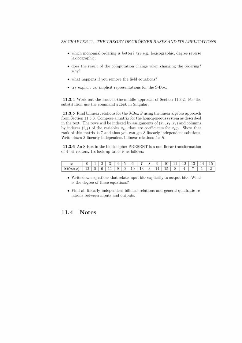
380CHAPTER 11. THE THEORY OF GROBNER BASES AND ITS APPLICATIONS
• which monomial ordering is better? try e.g. lexicographic, degree reverselexicographic;
• does the result of the computation change when changing the ordering?why?
• what happens if you remove the field equations?
• try explicit vs. implicit representations for the S-Box;
11.3.4 Work out the meet-in-the-middle approach of Section 11.3.2. For thesubstitution use the command subst in Singular.
11.3.5 Find bilinear relations for the S-Box S using the linear algebra approachfrom Section 11.3.3. Compose a matrix for the homogeneous system as describedin the text. The rows will be indexed by assignments of (x0, x1, x2) and columnsby indexes (i, j) of the variables ai,j that are coefficients for xiyj . Show thatrank of this matrix is 7 and thus you can get 3 linearly independent solutions.Write down 3 linearly independent bilinear relations for S.
11.3.6 An S-Box in the block cipher PRESENT is a non-linear transformationof 4-bit vectors. Its look-up table is as follows:
x 0 1 2 3 4 5 6 7 8 9 10 11 12 13 14 15SBox(x) 12 5 6 11 9 0 10 13 3 14 15 8 4 7 1 2
• Write down equations that relate input bits explicitly to output bits. Whatis the degree of these equations?
• Find all linearly independent bilinear relations and general quadratic re-lations between inputs and outputs.
11.4 Notes
Chapter 12
Coding theory withcomputer algebra packages
Stanislav Bulygin
In this chapter we give a brief overview of the three computer algebra systems:Singular, Magma, and GAP. We concentrate our attention on things that areuseful for the book. On other topics, as well as language semantics and syntaxthe reader is referred to the corresponding web-cites.
12.1 Singular
As is cited at www.singular.uni-kl.de: “SINGULAR is a Computer AlgebraSystem for polynomial computations with special emphasis on the needs of com-mutative algebra, algebraic geometry, and singularity theory”. In the contextof this book, we use some functionality provided for AG-codes (brnoeth.lib),decoding linear code via polynomial system solving (decodegb.lib), teachingcryptography (crypto.lib, atkins.lib) and Grobner bases (teachstd.lib).Singular can be downloaded free of charge from http://www.singular.uni-kl.
de/download.html for different platforms (Linux, Windows, Mac OS). The cur-rent version is 3-0-4 *** to change at the end *** The web-cite provides an onlinemanual at http://www.singular.uni-kl.de/Manual/ latest/index.htm. Be-low we provide the list of commands that can be used to work with objectspresented in this book together with short descriptions. Examples of use can belooked at from the links given below. More examples occur throughout the bookat the corresponding places. The functionality mentioned above is provided vialibraries and not the kernel function to load a library in Singular one has totype (brnoeth.lib as an example):> LIB"brnoeth.lib";
brnoeth.lib: Brill-Noether Algorithm, Weierstrass-SG and AG-codes by J.I. Farran Martin and C. Lossen (http://www.singular.uni-kl.de/Manual/latest/sing_1238.htm#SEC1297)Description: Implementation of the Brill-Noether algorithm for solving the
381
382CHAPTER 12. CODING THEORY WITH COMPUTER ALGEBRA PACKAGES
Riemann-Roch problem and applications in Algebraic Geometry codes. Thecomputation of Weierstrass semigroups is also implemented. The proceduresare intended only for plane (singular) curves defined over a prime field of pos-itive characteristic. For more information about the library see the end of thefile brnoeth.lib.Selected procedures:
- NSplaces: computes non-singular places with given degrees
- BrillNoether: computes a vector space basis of the linear system L(D)
- Weierstrass: computes the Weierstrass semigroup of C at P up to m
- AGcode_L: computes the evaluation AG code with divisors G and D
- AGcode_Omega: computes the residual AG code with divisors G and D
- decodeSV: decoding of a word with the basic decoding algorithm
- dual_code: computes the dual code
decodegb.lib: Decoding and minimum distance of linear codes with Grobnerbases by S. Bulygin (...)Description: In this library we generate several systems used for decoding cycliccodes and finding their minimum distance. Namely, we work with the Cooper’sphilosophy and generalized Newton identities. The original method of quadraticequations is worked out here as well. We also (for comparison) enable to workwith the system of Fitzgerald-Lax. We provide some auxiliary functions for fur-ther manipulations and decoding. For an overview of the methods mentionedabove, see “Decoding codes with GB” section of the manual. For the vanishingideal computation the algorithm of Farr and Gao is implemented.Selected procedures:
- sysCRHT: generates the CRHT-ideal as in Cooper’s philosophy
- sysNewton: generates the ideal with the generalized Newton identities
- syndrome: computes a syndrome w.r.t. the given check matrix
- sysQE: generates the system of quadratic equations for decoding
- errorRand: inserts random errors in a word
- randomCheck: generates a random check matrix
- mindist: computes the minimum distance of a code
- decode: decoding of a word using the system of quadratic equations
- decodeRandom: a procedure for manipulation with random codes
- decodeCode: a procedure for manipulation with the given code
- vanishId: computes the vanishing ideal for the given set of points
12.2. MAGMA 383
crypto.lib: Procedures for teaching cryptography by G. Pfister (http: //www.singular.uni-kl.de/Manual/latest/sing_1295.htm#SEC1354)Description: The library contains procedures to compute the discrete logarithm,primality-tests, factorization included elliptic curve methodes. The library isintended to be used for teaching purposes but not for serious computations.Sufficiently high printlevel allows to control each step, thus illustrating thealgorithms at work.atkins.lib: Procedures for teaching Elliptic Curve cryptography (primalitytest) by S. Steidel (http://www.singular.uni-kl.de/Manual/latest/sin g_1281.htm#SEC1340)Description: The library contains auxiliary procedures to compute the ellipticcurve primality test of Atkin and the Atkin’s Test itself. The library is intendedto be used for teaching purposes but not for serious computations. Sufficientlyhigh printlevel allows to control each step, thus illustrating the algorithms atwork. teachstd.lib: Procedures for teaching standard bases by G.-M. Greuel(http://www.singular.uni-kl.de/Manual/latest/sing_1344.htm#SEC1403)Description: The library is intended to be used for teaching purposes, but notfor serious computations. Sufficiently high printlevel allows to control eachstep, thus illustrating the algorithms at work. The procedures are implementedexactly as described in the book ’A SINGULAR Introduction to CommutativeAlgebra’ by G.-M. Greuel and G. Pfister (Springer 2002) [].Selected procedures:
- tail: tail of f
- leadmonomial: leading monomial as poly (also for vectors)
- monomialLcm: lcm of monomials m and n as poly (also for vectors)
- spoly: s-polynomial of f [symmetric form]
- NFMora normal form of i w.r.t Mora algorithm
- prodcrit: test for product criterion
- chaincrit: test for chain criterion
- standard: standard basis of ideal/module
12.2 Magma
“Magma is a large, well-supported software package designed to solve computa-tionally hard problems in algebra, number theory, geometry and combinatorics”– this is a formulation given at the official web-site http://magma.maths.usyd.edu.au/magma/. The current version is 2.15-7 *** to change at the end ***.In this book we use illustrations with Magma for different coding construc-tions: general, as well as more specific, such as AG-codes, also some machineryfor working with algebraic curves, as well as a few procedures for cryptog-raphy. Although Magma is a non-commercial system, it is still not free ofcharge: one has to purchase a license to work with it. Details can be found athttp://magma.maths.usyd.edu.au/magma/Ordering/ordering.shtml. Stillone can try to run simple Magma-code in the so-called “Magma-Calculator”
384CHAPTER 12. CODING THEORY WITH COMPUTER ALGEBRA PACKAGES
(http://magma.maths.usyd.edu.au/calc/). *** All examples and exercisesrun successfully in this calculator. *** Online help system for Magma canbe found at http://magma.maths.usyd.edu.au/magma/htmlhelp/MAGMA.htm.Next we describe briefly some procedures that come in hand while dealing withobjects from this book. We list only a few commands to give a flavor of func-tionality. One can get a lot more from the manual.
12.2.1 Linear codes
Full list of commands with descriptions can be found at http://magma.maths.usyd.edu.au/magma/htmlhelp/text1667.htm
- LinearCode: constructs a linear codes as a vector subspace
- PermutationCode: permutes positions in a code
- RepetitionCode: constructs a repetition code
- RandomLinearCode: constructs random linear code
- CyclicCode constructs a cyclic code
- ReedMullerCode: constructs a Reed-Muller code
- HammingCode: constructs a Hamming code
- BCHCode: constructs a BCH code
- ReedSolomonCode: constructs a Reed-Solomon code
- GeneratorMatrix: yields the generator matrix
- ParityCheckMatrix: yields the parity check matrix
- Dual: constructs the dual code
- GeneratorPolynomial: yields the generator polynomial of the given cycliccode
- CheckPolynomial: yields the check polynomial of the given cyclic code
- Random: yields a random codeword
- Syndrome: yields a syndrome of a word
- Distance: yields distance between words
- MinimumDistance: computes minimum distance of a code
- WeightEnumerator: computes the weight enumerator of a code
- ProductCode: constructs a product code from the given two
- SubfieldSubcode: constructs a subfield subcode
- McEliecesAttack: Runs basic attack on the McEliece cryptosystem
- GriesmerBound: provides the Griesmer bound for the given parameters
12.2. MAGMA 385
- SpherePackingBound: provides the sphere packing bound for the givenparameters
- BCHBound: provides the BCH bound for the given cyclic code
- Decode: decode a code with standard methods
- MattsonSolomonTransform: computes the Mattson-Solomon transform
- AutomorphismGroup: computes the automorphism group of the given code
12.2.2 AG-codes
Full list of commands with descriptions can be found at http://magma.maths.usyd.edu.au/magma/htmlhelp/text1686.htm
- AGCode: constructs an AG-code
- AGDualCode: constructs a dual AG-code
- HermitianCode: constructs a Hermitian code
- GoppaDesignedDistance: returns designed Goppa distance
- AGDecode: basic algorithm for decoding an AG-code
12.2.3 Algebraic curves
Full list of commands with descriptions can be found at http://magma.maths.usyd.edu.au/magma/htmlhelp/text1686.htm
- Curve: constructs a curve
- CoordinateRing: computes the coordinate ring of the given curve withGrobner basis techniques
- JacobianMatrix: computes the Jacobian matrix
- IsSingular: test if the given curve has singularities
- Genus: computes genus of a curve
- EllipticCurve: constructs an elliptic curve
- AutomorphismGroup: computes the automorphism of the given curve
- FunctionField: computes the function field of the given curve
- Valuation: computes a valuation of the given function w.r.t the givenplace
- GapNumbers:: yields gap numbers
- Places: computes places of the given curve
- RiemannRochSpace: computes the Riemann-Roch space
386CHAPTER 12. CODING THEORY WITH COMPUTER ALGEBRA PACKAGES
- Basis: computes a sequence containing a basis of the Riemann-Roch spaceL(D) of the divisor D.
- CryptographicCurve: given the finite field computes an elliptic curve Eover a finite field together with a point P on E such that the order of P isa large prime and the pair (E,P ) satisfies the standard security conditionsfor being resistant to MOV and Anomalous attacks
12.3 GAP
In this subsection we consider GAP computational discrete algebra system thatis “a system for computational discrete algebra, with particular emphasis onComputational Group Theory”. GAP stands for Groups, Algorithms, Pro-gramming, http://www.gap-system.org. Although primary concern of GAP iscomputations with groups, it also provides coding-oriented functionality via theGUAVA package, http://www.gap-system.org/Packages/guava.html. GAPcan be downloaded for free from http://www.gap-system.org/Download/index.
html. The current GAP version is 4.4.12, the current GUAVA version is 3.9.*** to change at the end *** As before, we only list here some proceduresto provide an understanding of which things can be done with GUAVA/GAP.Package GUAVA is included as follows:> LoadPackage("guava");
Online manual for guava can be found at http://www.gap-system.org/Manuals/pkg/guava3.9/htm/chap0.html
Selected procedures:
- RandomLinearCode: constructs a random linear code
- GeneratorMatCode: constructs a linear code via its generator matrix
- CheckMatCode: constructs a linear code via its parity check matrix
- HammingCode: constructs a Hamming code
- ReedMullerCode: constructs a Reed-Muller code
- GeneratorPolCode: constructs a cyclic code via its generator polynomial
- CheckPolCode: constructs a cyclic code via its check polynomial
- RootsCode: constructs a cyclic code via roots of the generator polynomial
- BCHCode: constructs a BCH code
- ReedSolomomCode: constructs a Reed-Solomon code
- CyclicCodes: returns all cyclic codes of given length
- EvaluationCode: construct an evaluation code
- AffineCurve: sets a framework for working with an affine curve
- GoppaCodeClassical: construct a classical geometric Goppa code
- OnePointAGCode: construct a one-point AG-code
12.4. SAGE 387
- PuncturedCode: construct a punctured code for the given
- DualCode: constructs the dual code to the given
- UUVCode: constructs a code via the (u|u+ v)-construction
- LowerBoundMinimumDistance: yields the best lower bound on the mini-mum distance available
- UpperBoundMinimumDistance: yields the best upper bound on the mini-mum distance available
- MinimumDistance: yields the minimum distance of the given code
- WeightDistribution: yield the weight distribution of the given code
- Decode: general decoding procedure
12.4 Sage
Sage framework provides an opportunity to use strengths of many open-sourcecomputer algebra systems (among them are Singular and GAP) for developingeffective code for solving different mathematical problems. The general frame-work is made possible through the python-interface. Sage is thought as an open-source alternative to commercial systems, such as Magma, Maple, Mathematica,and Matlab. Sage provides tools for a wide variety of algebraic and combina-torial objects among other things. For example functionality for coding theoryand cryptography is present, as well as functionality for working with algebraiccurves. The web-page of the project is http://www.sagemath.org/. One candownload Sage from http://www.sagemath.org/download.html. The refer-ence manual for Sage is available at http://www.sagemath.org/doc/reference/.Now we briefly describe some commands that may come in hand while workingwith this book.
12.4.1 Coding Theory
Manual available at http://www.sagemath.org/doc/reference/coding.htmlCoding-functionality of Sage has a lot in common with the one of GAP/GUAVA.In fact, for many commands Sage uses implementations available from GAP.Selected procedures:
- LinearCodeFromCheckMatrix: constructs a linear code via its parity checkmatrix
- RandomLinearCode: constructs a random linear code
- CyclicCodeFromGeneratingPolynomial: constructs a cyclic code via itsgenerator polynomial
- QuadraticResidueCode: constricts a quadratic residue cyclic code
- ReedSolomonCode: constructs a Reed-Solomon code
388CHAPTER 12. CODING THEORY WITH COMPUTER ALGEBRA PACKAGES
- gilbert_lower_bound: computes the lower bound due to Gilbert
- permutation_automorphism_group: computes the permutation automor-phism group of the given code
- weight_distribution: computes the weight distribution of a code
12.4.2 Cryptography
Manual available at http://www.sagemath.org/doc/reference/cryptography.htmlSelected procedures/classes:
- SubstitutionCryptosystem: defines a substitution cryptosystem/cipher
- VigenereCryptosystem: defines the Vigenere cryptosystem/cipher
- lfsr_sequence: produces an output of the given LFSR
- SR: returns a small scale variant for the AES
12.4.3 Algebraic curves
Manual available at http://www.sagemath.org/doc/reference/plane_curves.htmlSelected procedures/classes:
- EllipticCurve_finite_field: constructs an elliptic curves over a finitefield
- trace_of_frobenius: computes the trace of Frobenius of an elliptic curve
- cardinality: computes the number of rational points of an elliptic curve
- HyperellipticCurve_finite_field: constructs a hyperelliptic curvesover a finite field
12.5 Coding with computer algebra
12.5.1 Introduction
..............
12.5.2 Error-correcting codes
Example 12.5.1 Let us construct Example 2.1.6 for n = 5 using GAP/GUAVA.First, we need to define the list of codewords> M := Z(2)^0 * [
> [1,1,0,0,0],[1,0,1,0,0],[1,0,0,1,0],[1,0,0,0,1],[0,1,1,0,0],
> [0,1,0,1,0],[0,1,0,0,1],[0,0,1,1,0],[0,0,1,0,1],[0,0,0,1,1]
> ];
In GAP Z(q) is a primitive element of the field GF(q). So multiplying the listM by Z(2)^0 we make sure that the elements belong to GF(2). Now constructthe code:> C:=ElementsCode(M,"Example 2.1.6 for n=5",GF(2));
12.5. CODING WITH COMPUTER ALGEBRA 389
a (5,10,1..5)1..5 Example 2.1.6 for n=5 over GF(2)
We can compute the minimum distance and the size of C as follows> MinimumDistance(C);
2
> Size(C);
10
Now the information on the code is updated> Print(C);
a (5,10,2)1..5 Example 2.1.6 for n=5 over GF(2)
The block 1..5 gives a range for the covering radius of C. We treat it later in3.2.24.
Example 12.5.2 Let us construct the Hamming [7, 4, 3] code in GAP/GUAVAand Magma. Both systems have a built-in command for this. In GAP>C:=HammingCode(3,GF(2));
a linear [7,4,3]1 Hamming (3,2) code over GF(2)
Here the syntax is HammingCode(r,GF(q)) where r is the redundancy and GF(q)
is the defining alphabet. We can extract a generator matrix as follows> M:=GeneratorMat(C);;
> Display(M);
1 1 1 . . . .
1 . . 1 1 . .
. 1 . 1 . 1 .
1 1 . 1 . . 1
Two semicolons indicate that we do not want an output of a command be printedon the screen. Display provides a nice way to represent objects.In Magma we do it like this> C:=HammingCode(GF(2),3);
> C;
[7, 4, 3] "Hamming code (r = 3)" Linear Code over GF(2)
Generator matrix:
[1 0 0 0 1 1 0]
[0 1 0 0 0 1 1]
[0 0 1 0 1 1 1]
[0 0 0 1 1 0 1]
So here the syntax is reverse.
Example 12.5.3 Let us construct [7, 4, 3] binary Hamming code via its paritycheck matrix. In GAP/GUAVA we proceed as follows> H1:=Z(2)^0*[[1,0,0],[0,1,0],[0,0,1],[1,1,0],[1,0,1],[0,1,1],[1,1,1]];;
> H:=TransposedMat(H1);;
> C:=CheckMatCode(H,GF(2));
a linear [7,4,1..3]1 code defined by check matrix over GF(2)
We can now check the property of the check matrix:> G:=GeneratorMat(C);;
> Display(G*H1);
. . .
. . .
. . .
. . .
390CHAPTER 12. CODING THEORY WITH COMPUTER ALGEBRA PACKAGES
We can also compute syndromes:> c:=CodewordNr(C,7);
[ 1 1 0 0 1 1 0 ]
> Syndrome(C,c);
[ 0 0 0 ]
> e:=Codeword("1000000");;
> Syndrome(C,c+e);
[ 1 0 0 ]
So we have taken the 7th codeword in the list of codewords of C and showedthat its syndrome is 0. Then we introduced an error at the first position: thesyndrome is non-zero.In Magma one can generate codes only by vector subspace generators. So theway to generate a code via its parity check matrix is to use Dual command, seeExample 12.5.4. So we construct the Hamming code as in Example 12.5.2 andthen proceed as above.> C:=HammingCode(GF(2),3);
> H:=ParityCheckMatrix(C);
> H;
[1 0 0 1 0 1 1]
[0 1 0 1 1 1 0]
[0 0 1 0 1 1 1]
> G:=GeneratorMatrix(C);
> G*Transpose(H);
[0 0 0]
[0 0 0]
[0 0 0]
[0 0 0]
Syndromes are handled as follows:> c:=Random(C);
> Syndrome(c,C);
(0 0 0)
> V:=AmbientSpace(C);
> e:=V![1,0,0,0,0,0,0];
> r:=c+e;
> Syndrome(r,C);
(1 0 0)
Here we have taken a random codeword of C and computed its syndrome. Now,V is the space where C is defined, so the error vector e sits there, which isindicated by the prefix V!.
Example 12.5.4 Let us start again with the binary Hamming code and seehow dual codes are constructed in GAP and Magma. In GAP we have> C:=HammingCode(3,GF(2));;
> CS:=DualCode(C);
a linear [7,3,4]2..3 dual code
> G:=GeneratorMat(C);;
> H:=GeneratorMat(CS);;
> Display(G*TransposedMat(H));
. . .
. . .
12.5. CODING WITH COMPUTER ALGEBRA 391
. . .
. . .
The same can be done in Magma. Moreover, we can make sure that the dual ofthe Hamming code is the predefined simplex code:> C:=HammingCode(GF(2),3);
> CS:=Dual(C);
> G:=GeneratorMatrix(CS);
> S:=SimplexCode(3);
> H:=ParityCheckMatrix(S);
> G*Transpose(H);
[0 0 0 0]
[0 0 0 0]
[0 0 0 0]
Example 12.5.5 Let us work out some examples in GAP and Magma that il-lustrate the notions of permutation equivalency and permutation automorphismgroup. As a model example we take as usual the binary Hamming code. Nextwe show how equivalency can be checked in GAP/GUAVA:> C:=HammingCode(3,GF(2));;
> p:=(1,2,3)(4,5,6,7);;
> CP:=PermutedCode(C,p);
a linear [7,4,3]1 permuted code
> IsEquivalent(C,CP);
true
So codes C and CP are equivalent. We may compute the permutation that bringsC to CP:> CodeIsomorphism( C, CP );
(4,5)
Interestingly, we obtain that CP can be obtained from C just by (4,5). Let ascheck if this is indeed true:> CP2:=PermutedCode(C,(4,5));;
> Display(GeneratorMat(CP)*TransposedMat(CheckMat(CP2)));
. . .
. . .
. . .
. . .
So indeed the codes CP and CP2 are the same. The permutation automorphismgroup can be computed via:> AG:=AutomorphismGroup(C);
Group([ (1,2)(5,6), (2,4)(3,5), (2,3)(4,6,5,7), (4,5)(6,7), (4,6)(5,7) ])
> Size(AG)
168
So the permutation automorphism group of C has 5 generators and 168 elements.In Magma there is no immediate way to define permuted codes. We still cancompute a permutation automorphism group, which is called a permutationgroup there:> C:=HammingCode(GF(2),3);
> PermutationGroup(C);
Permutation group acting on a set of cardinality 7
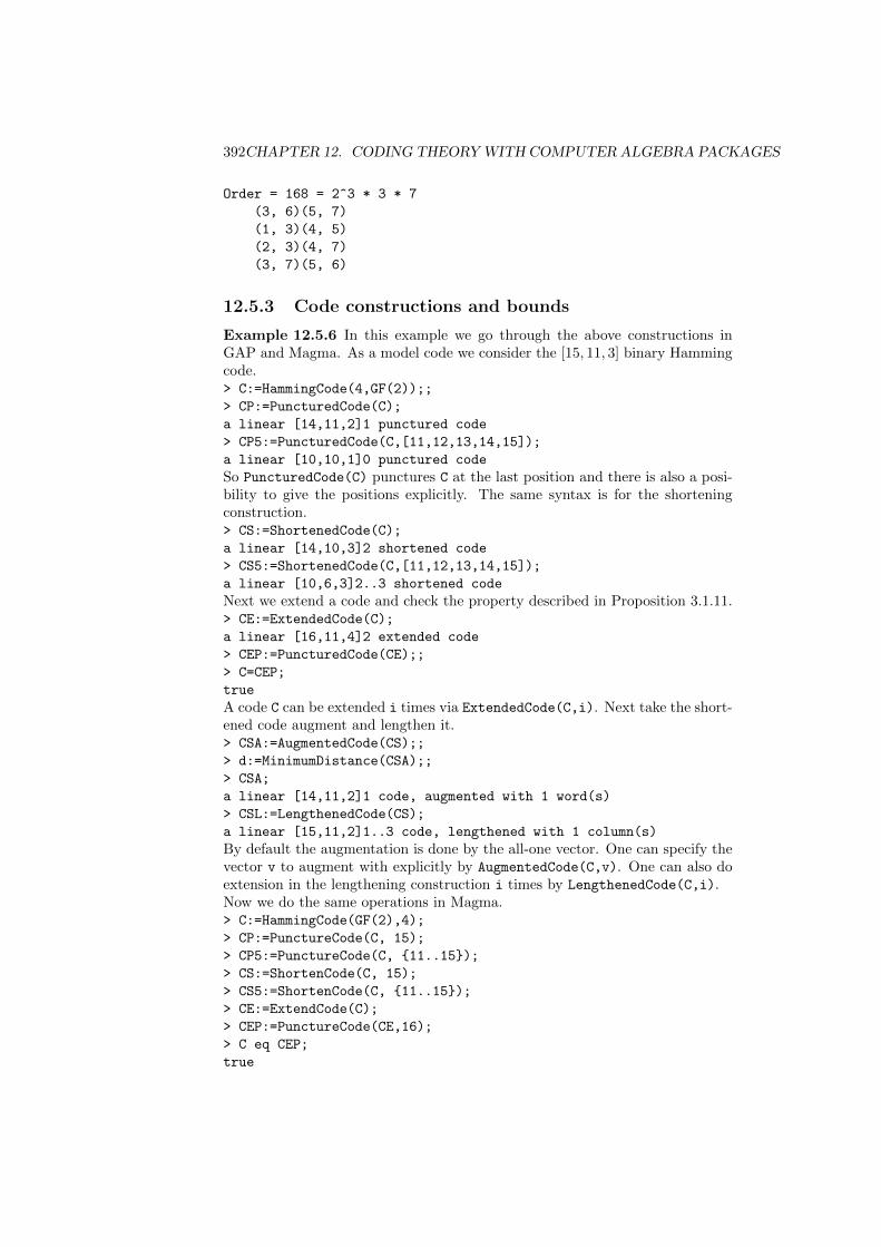
392CHAPTER 12. CODING THEORY WITH COMPUTER ALGEBRA PACKAGES
Order = 168 = 2^3 * 3 * 7
(3, 6)(5, 7)
(1, 3)(4, 5)
(2, 3)(4, 7)
(3, 7)(5, 6)
12.5.3 Code constructions and bounds
Example 12.5.6 In this example we go through the above constructions inGAP and Magma. As a model code we consider the [15, 11, 3] binary Hammingcode.> C:=HammingCode(4,GF(2));;
> CP:=PuncturedCode(C);
a linear [14,11,2]1 punctured code
> CP5:=PuncturedCode(C,[11,12,13,14,15]);
a linear [10,10,1]0 punctured code
So PuncturedCode(C) punctures C at the last position and there is also a posi-bility to give the positions explicitly. The same syntax is for the shorteningconstruction.> CS:=ShortenedCode(C);
a linear [14,10,3]2 shortened code
> CS5:=ShortenedCode(C,[11,12,13,14,15]);
a linear [10,6,3]2..3 shortened code
Next we extend a code and check the property described in Proposition 3.1.11.> CE:=ExtendedCode(C);
a linear [16,11,4]2 extended code
> CEP:=PuncturedCode(CE);;
> C=CEP;
true
A code C can be extended i times via ExtendedCode(C,i). Next take the short-ened code augment and lengthen it.> CSA:=AugmentedCode(CS);;
> d:=MinimumDistance(CSA);;
> CSA;
a linear [14,11,2]1 code, augmented with 1 word(s)
> CSL:=LengthenedCode(CS);
a linear [15,11,2]1..3 code, lengthened with 1 column(s)
By default the augmentation is done by the all-one vector. One can specify thevector v to augment with explicitly by AugmentedCode(C,v). One can also doextension in the lengthening construction i times by LengthenedCode(C,i).Now we do the same operations in Magma.> C:=HammingCode(GF(2),4);
> CP:=PunctureCode(C, 15);
> CP5:=PunctureCode(C, 11..15);
> CS:=ShortenCode(C, 15);
> CS5:=ShortenCode(C, 11..15);
> CE:=ExtendCode(C);
> CEP:=PunctureCode(CE,16);
> C eq CEP;
true
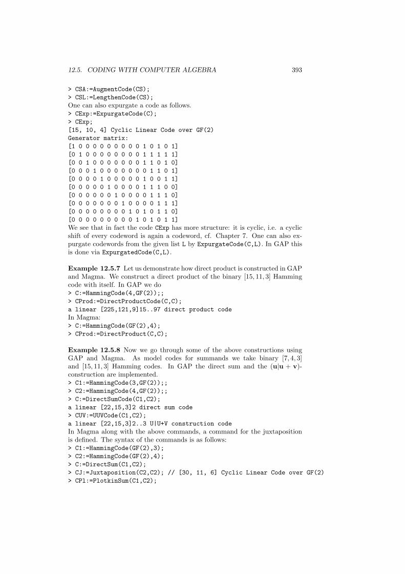
12.5. CODING WITH COMPUTER ALGEBRA 393
> CSA:=AugmentCode(CS);
> CSL:=LengthenCode(CS);
One can also expurgate a code as follows.> CExp:=ExpurgateCode(C);
> CExp;
[15, 10, 4] Cyclic Linear Code over GF(2)
Generator matrix:
[1 0 0 0 0 0 0 0 0 0 1 0 1 0 1]
[0 1 0 0 0 0 0 0 0 0 1 1 1 1 1]
[0 0 1 0 0 0 0 0 0 0 1 1 0 1 0]
[0 0 0 1 0 0 0 0 0 0 0 1 1 0 1]
[0 0 0 0 1 0 0 0 0 0 1 0 0 1 1]
[0 0 0 0 0 1 0 0 0 0 1 1 1 0 0]
[0 0 0 0 0 0 1 0 0 0 0 1 1 1 0]
[0 0 0 0 0 0 0 1 0 0 0 0 1 1 1]
[0 0 0 0 0 0 0 0 1 0 1 0 1 1 0]
[0 0 0 0 0 0 0 0 0 1 0 1 0 1 1]
We see that in fact the code CExp has more structure: it is cyclic, i.e. a cyclicshift of every codeword is again a codeword, cf. Chapter 7. One can also ex-purgate codewords from the given list L by ExpurgateCode(C,L). In GAP thisis done via ExpurgatedCode(C,L).
Example 12.5.7 Let us demonstrate how direct product is constructed in GAPand Magma. We construct a direct product of the binary [15, 11, 3] Hammingcode with itself. In GAP we do> C:=HammingCode(4,GF(2));;
> CProd:=DirectProductCode(C,C);
a linear [225,121,9]15..97 direct product code
In Magma:> C:=HammingCode(GF(2),4);
> CProd:=DirectProduct(C,C);
Example 12.5.8 Now we go through some of the above constructions usingGAP and Magma. As model codes for summands we take binary [7, 4, 3]and [15, 11, 3] Hamming codes. In GAP the direct sum and the (u|u + v)-construction are implemented.> C1:=HammingCode(3,GF(2));;
> C2:=HammingCode(4,GF(2));;
> C:=DirectSumCode(C1,C2);
a linear [22,15,3]2 direct sum code
> CUV:=UUVCode(C1,C2);
a linear [22,15,3]2..3 U|U+V construction code
In Magma along with the above commands, a command for the juxtapositionis defined. The syntax of the commands is as follows:> C1:=HammingCode(GF(2),3);
> C2:=HammingCode(GF(2),4);
> C:=DirectSum(C1,C2);
> CJ:=Juxtaposition(C2,C2); // [30, 11, 6] Cyclic Linear Code over GF(2)
> CPl:=PlotkinSum(C1,C2);
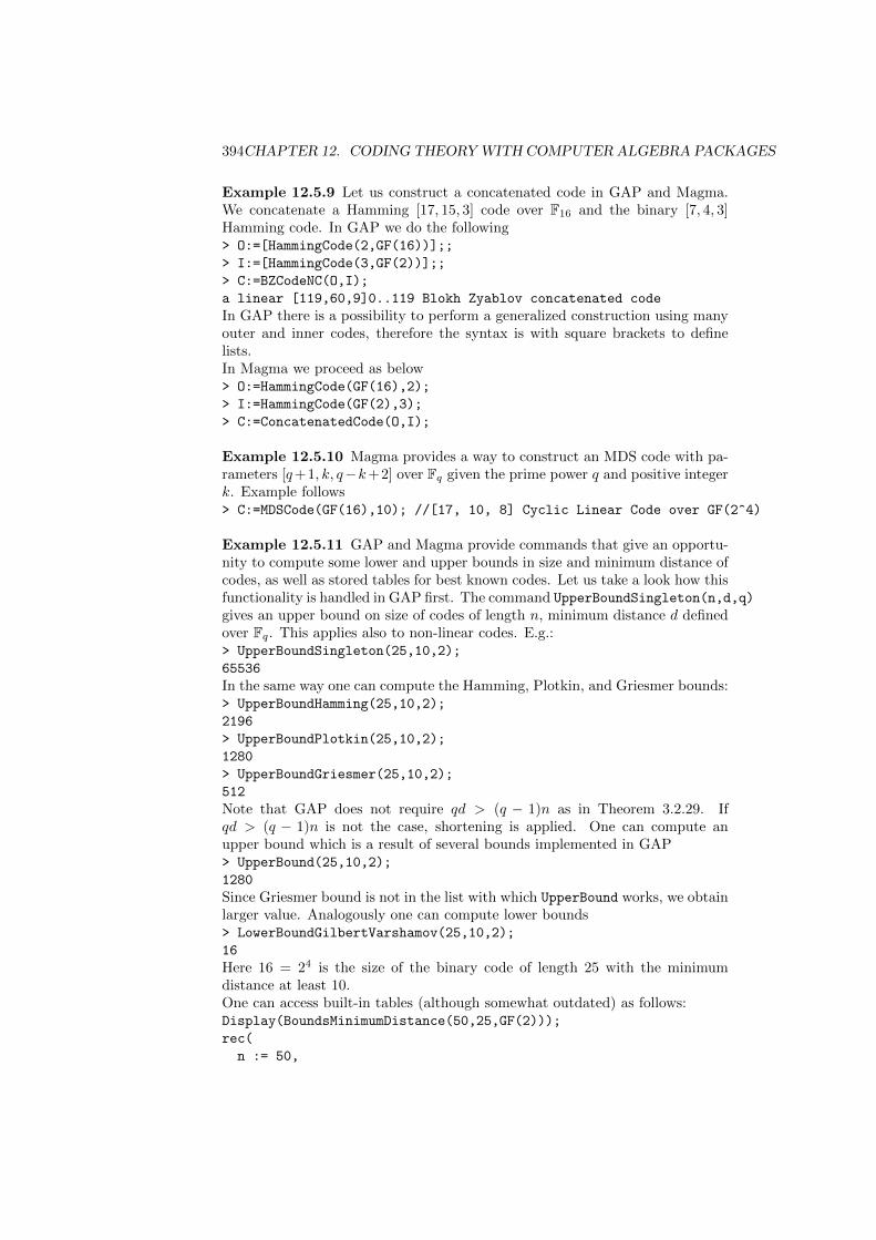
394CHAPTER 12. CODING THEORY WITH COMPUTER ALGEBRA PACKAGES
Example 12.5.9 Let us construct a concatenated code in GAP and Magma.We concatenate a Hamming [17, 15, 3] code over F16 and the binary [7, 4, 3]Hamming code. In GAP we do the following> O:=[HammingCode(2,GF(16))];;
> I:=[HammingCode(3,GF(2))];;
> C:=BZCodeNC(O,I);
a linear [119,60,9]0..119 Blokh Zyablov concatenated code
In GAP there is a possibility to perform a generalized construction using manyouter and inner codes, therefore the syntax is with square brackets to definelists.In Magma we proceed as below> O:=HammingCode(GF(16),2);
> I:=HammingCode(GF(2),3);
> C:=ConcatenatedCode(O,I);
Example 12.5.10 Magma provides a way to construct an MDS code with pa-rameters [q+1, k, q−k+2] over Fq given the prime power q and positive integerk. Example follows> C:=MDSCode(GF(16),10); //[17, 10, 8] Cyclic Linear Code over GF(2^4)
Example 12.5.11 GAP and Magma provide commands that give an opportu-nity to compute some lower and upper bounds in size and minimum distance ofcodes, as well as stored tables for best known codes. Let us take a look how thisfunctionality is handled in GAP first. The command UpperBoundSingleton(n,d,q)
gives an upper bound on size of codes of length n, minimum distance d definedover Fq. This applies also to non-linear codes. E.g.:> UpperBoundSingleton(25,10,2);
65536
In the same way one can compute the Hamming, Plotkin, and Griesmer bounds:> UpperBoundHamming(25,10,2);
2196
> UpperBoundPlotkin(25,10,2);
1280
> UpperBoundGriesmer(25,10,2);
512
Note that GAP does not require qd > (q − 1)n as in Theorem 3.2.29. Ifqd > (q − 1)n is not the case, shortening is applied. One can compute anupper bound which is a result of several bounds implemented in GAP> UpperBound(25,10,2);
1280
Since Griesmer bound is not in the list with which UpperBound works, we obtainlarger value. Analogously one can compute lower bounds> LowerBoundGilbertVarshamov(25,10,2);
16
Here 16 = 24 is the size of the binary code of length 25 with the minimumdistance at least 10.One can access built-in tables (although somewhat outdated) as follows:Display(BoundsMinimumDistance(50,25,GF(2)));
rec(
n := 50,
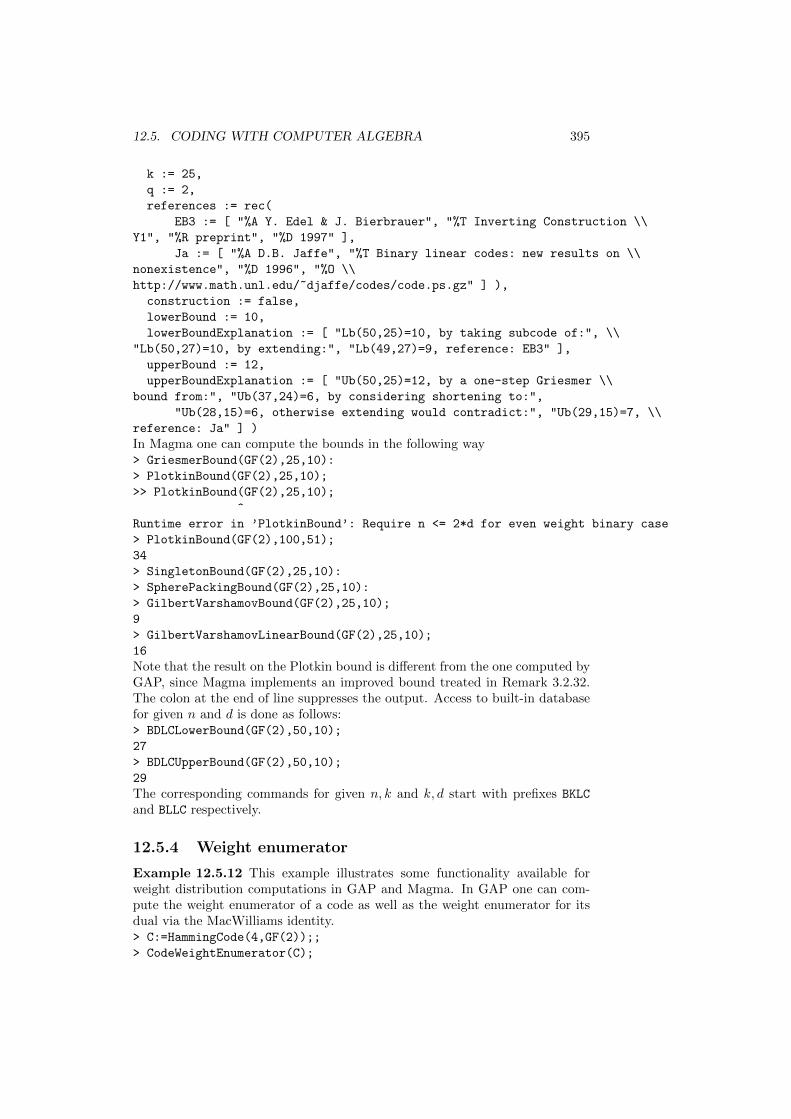
12.5. CODING WITH COMPUTER ALGEBRA 395
k := 25,
q := 2,
references := rec(
EB3 := [ "%A Y. Edel & J. Bierbrauer", "%T Inverting Construction \\
Y1", "%R preprint", "%D 1997" ],
Ja := [ "%A D.B. Jaffe", "%T Binary linear codes: new results on \\
nonexistence", "%D 1996", "%O \\
http://www.math.unl.edu/~djaffe/codes/code.ps.gz" ] ),
construction := false,
lowerBound := 10,
lowerBoundExplanation := [ "Lb(50,25)=10, by taking subcode of:", \\
"Lb(50,27)=10, by extending:", "Lb(49,27)=9, reference: EB3" ],
upperBound := 12,
upperBoundExplanation := [ "Ub(50,25)=12, by a one-step Griesmer \\
bound from:", "Ub(37,24)=6, by considering shortening to:",
"Ub(28,15)=6, otherwise extending would contradict:", "Ub(29,15)=7, \\
reference: Ja" ] )
In Magma one can compute the bounds in the following way> GriesmerBound(GF(2),25,10):
> PlotkinBound(GF(2),25,10);
>> PlotkinBound(GF(2),25,10);
^
Runtime error in ’PlotkinBound’: Require n <= 2*d for even weight binary case
> PlotkinBound(GF(2),100,51);
34
> SingletonBound(GF(2),25,10):
> SpherePackingBound(GF(2),25,10):
> GilbertVarshamovBound(GF(2),25,10);
9
> GilbertVarshamovLinearBound(GF(2),25,10);
16
Note that the result on the Plotkin bound is different from the one computed byGAP, since Magma implements an improved bound treated in Remark 3.2.32.The colon at the end of line suppresses the output. Access to built-in databasefor given n and d is done as follows:> BDLCLowerBound(GF(2),50,10);
27
> BDLCUpperBound(GF(2),50,10);
29
The corresponding commands for given n, k and k, d start with prefixes BKLC
and BLLC respectively.
12.5.4 Weight enumerator
Example 12.5.12 This example illustrates some functionality available forweight distribution computations in GAP and Magma. In GAP one can com-pute the weight enumerator of a code as well as the weight enumerator for itsdual via the MacWilliams identity.> C:=HammingCode(4,GF(2));;
> CodeWeightEnumerator(C);
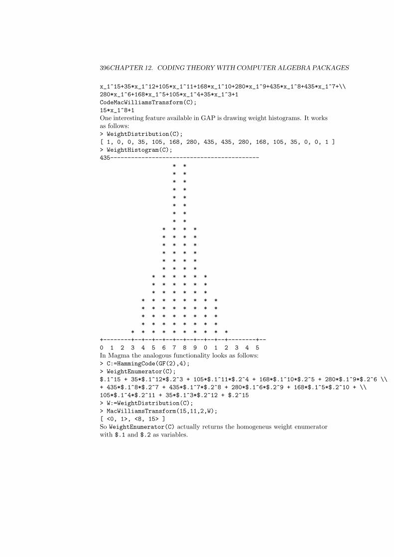
396CHAPTER 12. CODING THEORY WITH COMPUTER ALGEBRA PACKAGES
x_1^15+35*x_1^12+105*x_1^11+168*x_1^10+280*x_1^9+435*x_1^8+435*x_1^7+\\
280*x_1^6+168*x_1^5+105*x_1^4+35*x_1^3+1
CodeMacWilliamsTransform(C);
15*x_1^8+1
One interesting feature available in GAP is drawing weight histograms. It worksas follows:> WeightDistribution(C);
[ 1, 0, 0, 35, 105, 168, 280, 435, 435, 280, 168, 105, 35, 0, 0, 1 ]
> WeightHistogram(C);
435-------------------------------------------
* *
* *
* *
* *
* *
* *
* *
* *
* * * *
* * * *
* * * *
* * * *
* * * *
* * * *
* * * * * *
* * * * * *
* * * * * *
* * * * * * * *
* * * * * * * *
* * * * * * * *
* * * * * * * *
* * * * * * * * * *
+--------+--+--+--+--+--+--+--+--+--+--------+--
0 1 2 3 4 5 6 7 8 9 0 1 2 3 4 5
In Magma the analogous functionality looks as follows:> C:=HammingCode(GF(2),4);
> WeightEnumerator(C);
$.1^15 + 35*$.1^12*$.2^3 + 105*$.1^11*$.2^4 + 168*$.1^10*$.2^5 + 280*$.1^9*$.2^6 \\
+ 435*$.1^8*$.2^7 + 435*$.1^7*$.2^8 + 280*$.1^6*$.2^9 + 168*$.1^5*$.2^10 + \\
105*$.1^4*$.2^11 + 35*$.1^3*$.2^12 + $.2^15
> W:=WeightDistribution(C);
> MacWilliamsTransform(15,11,2,W);
[ <0, 1>, <8, 15> ]
So WeightEnumerator(C) actually returns the homogeneus weight enumeratorwith $.1 and $.2 as variables.
12.5. CODING WITH COMPUTER ALGEBRA 397
12.5.5 Codes and related structures
12.5.6 Complexity and decoding
Example 12.5.13 In GAP/GUAVA and Magma for general linear code theidea of Definition 2.4.10 (1) is employed. In GAP such a decoding goes asfollows> C:=RandomLinearCode(15,5,GF(2));;
> MinimumDistance(C);
5
> # can correct 2 errors
> c:="11101"*C; # encoding
> c in C;
true
> r:=c+Codeword("01000000100000");
> c1:=Decodeword(C,r);;
> c1 = c;
true
> m:=Decode(C,r); # obtain initial message word
[ 1 1 1 0 1 ]
One can also obtain the syndrome table that is a table of pairs coset leader /syndrome by SyndromeTable(C).The same idea is realized in Magma as follows.> C:=RandomLinearCode(GF(2),15,5); // can be [15,5,5] code
> # can correct 2 errors
> c:=Random(C);
> e:=AmbientSpace(C) ! [0,1,0,0,0,0,0,0,1,0,0,0,0,0,0];
> r:=c+e;
> result,c1:=Decode(C,r);
> result; // does decoding succeed?
true
> c1 eq c;
true
There are more advanced decoding methods for general linear codes. More onthat in Section 10.6.
12.5.7 Cyclic codes
Example 12.5.14 We have already constructed finite fields and worked withthem in GAP and Magma. Let us take a look one more time at those notionsand show some new. In GAP we handle finite fields as follows.> G:=GF(2^5);;
> a:=PrimitiveRoot(G);
Z(2^5)
> DefiningPolynomial(G);
x_1^5+x_1^2+Z(2)^0
a^5+a^2+Z(2)^0; # check
0*Z(2)
Pretty much the same funtionality is provided in Magma> G:=GF(2^5);
398CHAPTER 12. CODING THEORY WITH COMPUTER ALGEBRA PACKAGES
> a:=PrimitiveElement(G);
> DefiningPolynomial(G);
$.1^5+$.1^2+1
> b:=G.1;
> a eq b;
true
> // define explicitly
> P<x>:=PolynomialRing(GF(2));
> p:=x^5+x^2+1;
> F<z>:= ext<GF(2)|p>;
> F;
Finite field of size 2^5
Example 12.5.15 Minimal polynomials are computed in GAP as follows:> a:=PrimitiveUnityRoot(2,17);;
> MinimalPolynomial(GF(2),a);
x_1^8+x_1^7+x_1^6+x_1^4+x_1^2+x_1+Z(2)^0
In Magma it is done analogous> a:=RootOfUnity(17,GF(2));
> MinimalPolynomial(a,GF(2));
x^8 + x^7 + x^6 + x^4 + x^2 + x + 1
Example 12.5.16 Some example on how to compute the cyclotomic polyno-mial in GAP and Magma follow. In GAP> CyclotomicPolynomial(GF(2),10);
x_1^4+x_1^3+x_1^2+x_1+Z(2)^0
In Magma it is done as follows> CyclotomicPolynomial(10);
$.1^4 - $.1^3 + $.1^2 - $.1 + 1
Note that in Magma the cyclotomic polynomial is always defined over Q.
Example 12.5.17 Let us construct cyclic codes via roots in GAP and Magma.In GAP/GUAVA we proceed as follows.> C:=GeneratorPolCode(h,17,GF(2));; # h is from Example 6.1.41
> CR:=RootsCode(17,[1],2);;
> MinimumDistance(CR);;
> CR;
a cyclic [17,9,5]3..4 code defined by roots over GF(2)
> C=CR;
true
> C2:=GeneratorPolCode(g,17,GF(2));; # g is from Example 6.1.41
> CR2:=RootsCode(17,[3],2);;
> C2=CR2;
true
So we generated first a cyclic code which generator polynomial has a (predefined)primitive root of unity as a root. Then we took the first element, which is notin the cyclotomic class of 1 and that is 3. We constructed a cyclic code with aprimitive root of unity cubed as a root of the generator polynomial. Note thatthese results are in accordance with Example 12.5.15. We can also compute thenumber of all cyclic codes of the given length, as e.g.> NrCyclicCodes(17,GF(2));
12.5. CODING WITH COMPUTER ALGEBRA 399
8
In Magma we do the construction as follows> a:=RootOfUnity(17,GF(2));
> C:=CyclicCode(17,[a],GF(2));
Example 12.5.18 We can compute the Mattson-Solomon transform in Magma.This is done as follows:> F<x> := PolynomialRing(SplittingField(x^17-1));
> f:=x^15+x^3+x;
> A:=MattsonSolomonTransform(f,17);
> A;
$.1^216*x^16 + $.1^177*x^15 + $.1^214*x^14 + $.1^99*x^13 + \\
$.1^181*x^12 + $.1^173*x^11 + $.1^182*x^10 + $.1^198*x^9 + \\
$.1^108*x^8 + $.1^107*x^7 + $.1^218*x^6 + $.1^91*x^5 + $.1^54*x^4\\
+ $.1^109*x^3 + $.1^27*x^2 + $.1^141*x + 1
> InverseMattsonSolomonTransform(A,17) eq f;
true
So for the construction we need a field that contains a primitive n-th root ofunity. We can also compute the inverse transform.
12.5.8 Polynomial codes
Example 12.5.19 Now we describe constructions of Reed-Solomon codes inGAP/ GUAVA and Magma. In GAP we proceed as follows:> C:=ReedSolomonCode(31,5);
a cyclic [31,27,5]3..4 Reed-Solomon code over GF(32)
A construction of the extended code is somewhat different from the one definedin Definition 8.1.6. GUAVA first constructs by ExtendedReedSolomonCode(n,d)
first ReedSolomonCode(n-1,d-1) and then extends it. The code is defined overGF(n), so n should be a prime power.> CE:=ExtendedReedSolomonCode(31,5);
a linear [31,27,5]3..4 extended Reed Solomon code over GF(31)
The generalized Reed-Solomon codes are handled as follows.> R:=PolynomialRing(GF(2^5));;
> a:=Z(2^5);;
> L:=List([1,2,3,6,7,10,12,16,20,24,25,29],i->Z(2^5)^i);;
> CG:=GeneralizedReedSolomonCode(L,4,R);;
So we define the polynomial ring R and the list of points L. Note that such aconstruction corresponds to the construction from Definition 8.1.10 with b = 1.In Magma we proceed as follows.> C:=ReedSolomonCode(31,5);
> a:=PrimitiveElement(GF(2^5));
> A:=[a^i:i in [1,2,3,6,7,10,12,16,20,24,25,29]];
> B:=[a^i:i in [1,2,1,2,1,2,1,2,1,2,1,2]];
> CG:=GRSCode(A,B,4);
So Magma give an opportunity to construct the generalized Reed-Solomon codeswith arbitrary b which entries are non-zero.
Example 12.5.20 In Magma one can compute subfield subcodes. This is doneas follows:
400CHAPTER 12. CODING THEORY WITH COMPUTER ALGEBRA PACKAGES
> a:=RootOfUnity(17,GF(2));
> C:=CyclicCode(17,[a],GF(2^8)); // splitting field size 2^8
> CSS:=SubfieldSubcode(C);
> C2:=CyclicCode(17,[a],GF(2));
> C2 eq CSS;
true
> CSS_4:=SubfieldSubcode(C,GF(4)); // [17, 13, 4] code over GF(2^2)
By default the prime subfield is taken for the construction.
Example 12.5.21 *** GUAVA slow!!! ***In Magma we can compute a trace code as is shown below:> C:=HammingCode(GF(16),3);
> CT:=Trace(C);
> CT:Minimal;
[273, 272] Linear Code over GF(2)
We can also specify a subfield to restrict to by giving it as a second parameterin Trace.
Example 12.5.22 In GAP/GUAVA in order to construct an alternant codewe proceed as follows> a:=Z(2^5);;
> P:=List([1,2,3,6,7,10,12,16,20,24,25,29],i->a^i);;
> B:=List([1,2,1,2,1,2,1,2,1,2,1,2],i->a^i);;
> CA:=AlternantCode(2,B,P,GF(2));
a linear [12,5,3..4]3..6 alternant code over GF(2)
By providing an extension field as the last parameter in AlternantCode, oneconstructs an extension code (as per Definition 8.2.1) of the one defined by thebase field (in our example it is GF(2)), rather than the restriction-constructionas in Definition 8.3.1.In Magma one proceeds as follows.> a:=PrimitiveElement(GF(2^5));
> A:=[a^i:i in [1,2,3,6,7,10,12,16,20,24,25,29]];
> B:=[a^i:i in [1,2,1,2,1,2,1,2,1,2,1,2]];
> CA:=AlternantCode(A,B,2);
> CG:=GRSCode(A,B,2);
> CGS:=SubfieldSubcode(Dual(CG));
> CA eq CGS;
true
Here one can add a desired subfield for the restriction as in Definition 8.3.1 viagiving it as another parameter at the end of the parameter list for AlternantCode.
Example 12.5.23 In GAP/GUAVA one can construct a Goppa code as fol-lows.> x:=Indeterminate(GF(2),"x");;
> g:=x^3+x+1;
> C:=GoppaCode(g,15);
a linear [15,3,7]6..8 classical Goppa code over GF(2)
So the Goppa code C is constructed over the field, where the polynomial g isdefined. There is also a possibility to provide the list of non-roots L explicitlyvia GoppaCode(g,L).In Magma one needs to provide the list L explicitly.
12.5. CODING WITH COMPUTER ALGEBRA 401
> P<x>:=PolynomialRing(GF(2^5));
> G:=x^3+x+1;
> a:=PrimitiveElement(GF(2^5));
> L:=[a^i : i in [0..30]];
> C:=GoppaCode(L,G);
> C:Minimal;
[31, 16, 7] "Goppa code (r = 3)" Linear Code over GF(2)
The polynomial G should be defined in the polynomial ring over the extension.The command C:Minimal only displays the description for C, no generator ma-trix is displayed.
Example 12.5.24 Now we show how binary Reed-Muller code can be con-structed in GAP/GUAVA and also we check the property from the previousproposition.> u:=5;;
> m:=7;;
> C:=ReedMullerCode(u,m);;
> C2:=ReedMullerCode(m-u-1,m);;
> CD:=DualCode(C);
> CD = C2;
true
In Magma one can do the above analogously:> u:=5;
> m:=7;
> C:=ReedMullerCode(u,m);
> C2:=ReedMullerCode(m-u-1,m);
> CD:=Dual(C);
> CD eq C2;
true
12.5.9 Algebraic decoding

402CHAPTER 12. CODING THEORY WITH COMPUTER ALGEBRA PACKAGES
Chapter 13
Bezout’s theorem and codeson plane curves
Ruud Pellikaan
In this section affine and projective plane curves are defined. Bezout’s theoremon the number of points in the intersection of two plane curves is proved. A classof codes from plane curves is introduced and the parameters of these codes aredetermined. Divisors and rational functions on plane curve will be discussed.
13.1 Affine and projective space
lines planes quadricscoordinate transformationspictures
13.2 Plane curves
Let F be a field and F its algebraic closure. By an affine plane curve over F wemean the set of points (x, y) ∈ F2 such that F (x, y) = 0, where F ∈ F[X,Y ].Here F = 0 is called the defining equation of the curve. The F-rational pointsof the curve with defining equation F = 0 are the points (x, y) ∈ F2 such thatF (x, y) = 0. The degree of the curve is the degree of F .Two plane curves with defining equations F = 0 and G = 0 have a componentin common with defining equation H = 0, if F and G have a nontrivial factorH in common, that is F = BH and G = AH for some A,B ∈ F[X,Y ], and thedegree of H is not zero.A curve with defining equation F = 0, F ∈ F[X,Y ], is called irreducible if F isnot divisible by any G ∈ F[X,Y ] such that 0 < deg(G) < deg(F ), and absolutelyirreducible if F is irreducible when considered as a polynomial in F[X,Y ].The partial derivative with respect to X of a polynomial F =
∑fijX
iY j isdefined by
FX =∑
ifijXi−1Y j .
403
404CHAPTER 13. BEZOUT’S THEOREM AND CODES ON PLANE CURVES
The partial derivative with respect to Y is defined similarly.A point (x, y) on an affine curve with equation F = 0 is singular if FX(x, y) =FY (x, y) = 0, where FX and FY are the partial derivatives of F with respect toX and Y , respectively. A regular point of a curve is a nonsingular point of thecurve. A regular point (x, y) on the curve has a well-defined tangent line to thecurve with equation
FX(x, y)(X − x) + FY (x, y)(Y − y) = 0.
Example 13.2.1 The curve with defining equation X2 + Y 2 = 0 can be con-sidered over any field. The polynomial X2 + Y 2 is irreducible in F3[X,Y ] butreducible in F9[X,Y ] and F5[X,Y ]. The point (0, 0) is an F-rational point ofthe curve over any field F, and it is the only singular point of this curve if thecharacteristic of F is not two.
A projective plane curve of degree d with defining equation F = 0 over F is theset of points (x : y : z) ∈ P2(F) such that F (x, y, z) = 0, where F ∈ F[X,Y, Z]is a homogeneous polynomial of degree d.Let F =
∑fijX
iY j ∈ F[X,Y ] be a polynomial of degree d. The homogenizationF ∗ of F is an element of F[X,Y, Z] and is defined by
F ∗ =∑
fijXiY jZd−i−j .
Then F ∗(X,Y, Z) = ZdF (X/Z, Y/Z). If F = 0 defines an affine plane curveof degree d, then F ∗ = 0 is the equation of the corresponding projective curve.A point at infinity of the affine curve with equation F = 0 is a point of theprojective plane in the intersection of the line at infinity and the projectivecurve with equation F ∗ = 0. So the points at infinity on the curve are all points(x : y : 0) ∈ P2(F) such that F ∗(x, y, 0) = 0.A projective plane curve is reducible, respectively absolutely irreducible, if itsdefining homogeneous polynomial is irreducible, respectively absolutely irre-ducible.A point (x : y : z) on a projective curve with equation F = 0 is singular ifFX(x, y, z) = FY (x, y, z) = FZ(x, y, z) = 0, and regular otherwise. Through aregular point (x : y : z) on the curve passes the tangent line with equation
FX(x, y, z)X + FY (x, y, z)Y + FZ(x, y, z)Z = 0.
If F ∈ F[X,Y, Z] is a homogeneous polynomial of degree d, then Euler’s equation
XFX + Y FY + ZFZ = dF
holds. So the two definitions of the tangent line to a curve in the affine andprojective plane are consistent with each other.A curve is called regular or nonsingular if all its points are regular. In Corol-lary 13.3.13 it will be shown that a regular projective plane curve is absolutelyirreducible.
Remark 13.2.2 Let F be a polynomial in F[X,Y ] of degree d. Suppose thatF has at least d+ 1 elements. Then there exists an affine change of coordinates
13.2. PLANE CURVES 405
such that the coefficients of Ud and V d in F (U, V ) are 1. This is seen as follows.The projective curve with the defining equation F ∗ = 0 intersects the line atinfinity in at most d points. Then there exist two F-rational points P and Q onthe line at infinity and not on the curve. Choose a projective transformationof coordinates which transforms P and Q into (1 : 0 : 0) and (0 : 1 : 0),respectively. This change of coordinates leaves the line at infinity invariant andgives a polynomial F (U, V ) such that the coefficients of Ud and V d are notzero. An affine transformation can now transform these coefficients into 1. Iffor instance F = X2Y + XY 2 ∈ F4[X,Y ] and α is a primitive element of F4,then X = U + αV and Y = αU + V gives F (U, V ) = U3 + V 3.Similarly, for all polynomials F,G ∈ F[X,Y ] of degree l and m there exists anaffine change of coordinates such that the coefficients of V l and V m in F (U, V )and G(U, V ), respectively, are 1.
Example 13.2.3 The Fermat curve Fm is a projective plane curve with defin-ing equation
Xm + Y m + Zm = 0.
The partial derivatives of Xm + Y m + Zm are mXm−1, mY m−1, and mZm−1.So considered as a curve over the finite field Fq, it is regular if m is relativelyprime to q.
Example 13.2.4 Suppose q = r2. The Hermitian curve Hr over Fq is definedby the equation
Ur+1 + V r+1 + 1 = 0.
The corresponding homogeneous equation is
Ur+1 + V r+1 +W r+1 = 0.
Hence it has r+ 1 points at infinity and it is the Fermat curve Fm over Fq withr = m − 1. The conjugate of a ∈ Fq over Fr is obtained by a = ar. So theequation can also be written as
UU + V V +WW = 0.
This looks like equating a Hermitian form over the complex numbers to zeroand explains the terminology.We will see in Section 3 that for certain constructions of codes on curves it isconvenient to have exactly one point at infinity. We will give a transformationsuch that the new equation of the Hermitian curve has this property. Choosean element b ∈ Fq such that br+1 = −1. There are exactly r + 1 of these,since q = r2. Let P = (1 : b : 0). Then P is a point of the Hermitian curve.The tangent line at P has equation U + brV = 0. Multiplying with b gives theequation V = bU . Substituting V = bU in the defining equation of the curvegives that W r+1 = 0. So P is the only intersection point of the Hermitiancurve and the tangent line at P . New homogeneous coordinates are chosen suchthat this tangent line becomes the line at infinity. Let X1 = W , Y1 = U andZ1 = bU − V . Then the curve has homogeneous equation
Xr+11 = brY r1 Z1 + bY1Z
r1 − Zr+1
1
406CHAPTER 13. BEZOUT’S THEOREM AND CODES ON PLANE CURVES
in the coordinates X1, Y1 and Z1. Choose an element a ∈ Fq such that ar +a =−1. There are r of these. Let X = X1, Y = bY1 + aZ1 and Z = Z1. Then thecurve has homogeneous equation
Xr+1 = Y rZ + Y Zr
with respect to X, Y and Z. Hence the Hermitian curve has affine equation
Xr+1 = Y r + Y
with respect to X and Y . This last equation has (0 : 1 : 0) as the only point atinfinity.To see that the number of affine Fq-rational points is r+(r+1)(r2−r) = r3 oneargues as follows. The right side of the equation Xr+1 = Y r + Y is the tracefrom Fq to Fr. The first r in the formula on the number of points correspondsto the elements of Fr. These are exactly the elements of Fq with zero trace. Theremaining term corresponds to the elements in Fq with a nonzero trace, sincethe equation Xr+1 = β, β ∈ F∗r , has exactly r + 1 solutions in Fq.
Example 13.2.5 The Klein curve has homogeneous equation
X3Y + Y 3Z + Z3X = 0.
More generally we define the curve Km by the equation
XmY + Y mZ + ZmX = 0.
Suppose thatm2−m+1 is relatively prime to q. The partial derivatives of the leftside of the equation are mXm−1Y +Zm, mY m−1Z +Xm and mZm−1X +Y m.Let (x : y : z) be a singular point of the curve Km. If m is divisible by thecharacteristic, then xm = ym = zm = 0. So x = y = z = 0, a contradiction. Ifm and q are relatively prime, then xmy = −mymz = m2zmx. So
(m2 −m+ 1)zmx = xmy + ymz + zmx = 0.
Therefore z = 0 or x = 0, since m2−m+ 1 is relatively prime to the character-istic. But z = 0 implies xm = −mym−1z = 0. Furthermore ym = −mzm−1x.So x = y = z = 0, which is a contradiction. Similarly x = 0 leads to a contra-diction. Hence Km is nonsingular if gcd(m2 −m+ 1, q) = 1.
13.3 Bezout’s theorem
The principal theorem of algebra says that a polynomial of degree m in one vari-able with coefficients in a field has at most m zeros. If the field is algebraicallyclosed and if the zeros are counted with multiplicities, then the total numberof zeros is equal to m. Bezout’s theorem is a generalization of the principaltheorem of algebra from one to several variables. It can be stated and provedin any number of variables. But only the two variable case will be treated, thatis to say the case of plane curves.
First we recall some wellknown notions from commutative algebra.
13.3. BEZOUT’S THEOREM 407
Let R be a commutative ring with a unit. An ideal I in R is called a primeideal if I 6= R and for all f, g ∈ R if fg ∈ I, then f ∈ I or g ∈ I.Let F be a field. Let F be a polynomial in F[X,Y ] which is not a constant, andlet I be the ideal in F[X,Y ] generated by F . Then I is a prime ideal if and onlyif F is irreducible.Let R be a commutative ring with a unit. A nonzero element f of R is called azero divisor if fg = 0 for some g ∈ R, g 6= 0. The ring R is called an integraldomain if it has no zero divisors.Let S be a commutative ring with a unit. Let I be an ideal in S. The factorring of S modulo I is denoted by S/I. Then I is a prime ideal if and only ifS/I is an integral domain.LetR be an integral domain. Define the relation∼ on the set of pairs (f, g)|f, g ∈R, g 6= 0 by (f1, g1) ∼ (f2, g2) if and only if there exists an h ∈ R, h 6= 0 suchthat f1g2h = g1f2h. This is an equivalence relation. Its classes are called frac-tions . The class of (f, g) is denoted by f/g or f
g and f is called the numeratorand g the denominator. The field of fractions or quotient field of R consists ofall fractions f/g where f, g ∈ R and g 6= 0 and is denoted by Q(R). This indeedis a field with addition and multiplication defined by
f1
g1+f2
g2=f1g2 + f2g1
g1g2and
f1
g1· f2
g2=f1f2
g1g2.
Example 13.3.1 The quotient field of the integers Z is the rationals Q. Thequotient field of the ring of polynomials F[X1, . . . , Xm] is called the field ofrational functions (in m variables) and is denoted by F(X1, . . . , Xm).
Remark 13.3.2 If R is a commutative ring with a unit, then matrices withentries in R and the determinant of a square matrix can be defined as whenR is a field. The usual properties for matrix addition and multiplication hold.If moreover R is an integral domain, then a square matrix M of size n hasdeterminant zero if and only if there exists a nonzero r ∈ Rn such that rM = 0.This is seen by considering the same statement over the quotient field Q(R),where it is true, and clearing denominators.
Furthermore we define an algebraic construction which is called the resultant oftwo polynomials that measures whether they have a factor in common.
Definition 13.3.3 Let R be a commutative ring with a unit. Then R[Y ] is thering of polynomials in one variable Y with coefficients in R. Let F and G betwo polynomials in R[Y ] of degree l and m, respectively. Then F =
∑li=0 fiY
i
and G =∑mj=0 gjY
j , where fi, gj ∈ R for all i, j. Define the Sylvester matrixSylv(F,G) of F and G as the square matrix of size l +m by
Sylv(F,G) =
f0 f1 . . . . fl 0 . . . 0 00 f0 f1 . . . . fl 0 . . . 0...
. . .. . .
. . .. . . · · ·
. . .. . .
...0 . . . 0 f0 f1 . . . . fl 00 0 . . . 0 f0 f1 . . . . flg0 g1 . . . . . gm 0 . 00 g0 g1 . . . . . gm 0 ....
. . .. . .
. . .. . . · · ·
. . .. . .
...0 . . . 0 g0 g1 . . . . . gm
.
408CHAPTER 13. BEZOUT’S THEOREM AND CODES ON PLANE CURVES
The first m rows consist of the cyclic shifts of the first row
f0 f1 . . . fl 0 . . . 0
and the last l rows consist of the cyclic shifts of row m+ 1
g0 g1 . . . gm 0 . . . 0 .
The determinant of Sylv(F,G) is called the resultant of F and G and is denotedby Res(F,G).
Proposition 13.3.4 If R is an integral domain and f and g are elements ofR[Y ], then Res(F,G) = 0 if and only if F and G have a nontrivial commonfactor.
Proof. If F and G have a nontrivial common factor, then F = BH and G =AH for some A,B and H in R[Y ], where H has nonzero degree. So AF = BGfor some A and B, where deg(A) < m = deg(G) and deg(B) < l = deg(F ).Write A =
∑aiY
i, F =∑fjY
j , B =∑brY
r and G =∑gsY
s. Rewrite theequation AF −BG = 0 as a system of equations∑
i+j=k
aifj −∑r+s=k
brgs = 0 for k = 0, 1, ..., l +m− 1,
or as a matrix equation
(a,−b)Sylv(F,G) = 0,
where a = (a0, a1, ..., am−1), and b = (b0, b1, ..., bl−1). Hence the rows of thematrix Sylv(F,G) are dependent in case F and G have a common factor and soits determinant is zero. Thus we have shown that if F and G have a nontrivialcommon factor, then Res(F,G) = 0. The converse is also true. This is provedby reversing the argument.
Corollary 13.3.5 If F is an algebraically closed field and F and G are elementsof F[Y ], then Res(F,G) = 0 if and only if F and G have a common zero in F.
After this introduction on the resultant, we are in a position to prove a weakform of Bezout’s theorem.
Proposition 13.3.6 Two plane curves of degree l and m that do not have acomponent in common, intersect in at most lm points.
Proof. A special case of Bezout is m = 1. A line, which is not a component ofa curve of degree l, intersects this curve in at most l points. Stated differently,suppose that F is a polynomial in X and Y with coefficients in a field F andhas degree l, and L is a nonconstant linear form. If F and L have more than lcommon zeros, then L divides F in F[X,Y ]. A more general special case is ifF is a product of linear terms. So if one of the curves is a union of lines andthe other curve does not contain any of these lines as a component, then thenumber of points in the intersection is at most lm. This follows from the abovespecial case. The third special case is: if G = XY − 1 and F is arbitrary. Then
13.3. BEZOUT’S THEOREM 409
the first curve can be parameterized by X = T, Y = 1/T ; substituting this inF gives a polynomial in T and 1/T of degree at most l, multiplying by T l givesa polynomial of degree at most 2l, and therefore the intersection of these twocurves has at most 2l points. It is not possible to continue like this, that is tosay by parameterizing the second curve by rational functions in T : X = X(T )and Y = Y (T ).
The proof of the general case uses elimination theory. Suppose that we have twoequations in two variables of degree l and m, respectively, and we eliminate onevariable. Then we get a polynomial in one variable of degree at most lm havingas zeros the first coordinates of common zeros of the two original polynomials.In geometric terms, we have two curves of degree l respectively m in the affineplane, and we project the points of the intersection to a line. If we can showthat we get at most lm points on this line and we can choose the projection insuch a way that no two points of the intersection project to one point on theline, then we are done.
We may assume that the field is algebraically closed, since by a common zero(x, y) of F and G, we mean a pair (x, y) ∈ F2 such that F (x, y) = G(x, y) = 0.Let F and G be polynomials in the variables X and Y of degree l and m,respectively, with coefficients in a field F, and which do not have a commonfactor in F[X,Y ]. Then they do not have a nontrivial common factor in R[Y ],where R = F[X], so Res(F,G) is not zero by Proposition 13.3.4. By Remark13.2.2 we may assume that, after an affine change of coordinates, F and Gare monic and have degree l and m, respectively, as polynomials in Y withcoefficients in F[X]. Hence F =
∑li=0 fiY
i and G =∑mj=0 gjY
j , where fi andgj are elements of F[X] of degree at most l − i and m − j, respectively, andfl = gm = 1. The square matrix Sylv(F,G) of size l + m has entries in F[X].Taking the determinant gives the resultant Res(F,G) which is an element ofR = F[X], that is to say a polynomial in X with coefficients in F.
The degree is at most lm. This can be seen by homogenizing F and G. ThenF ∗ =
∑li=1 f
′iyi where f ′i is a homogeneous polynomial in X and Z of degree
l − i, and similarly for G∗. The determinant D(X,Z) of the correspondingSylvester matrix is homogeneous of degree lm, since
D(TX, TZ) = T lmD(X,Z).
This is seen by dividing the rows and columns of the matrix by appropriatepowers of T .
We claim that the zeros of the polynomial Res(F,G) are exactly the projectionof all points in the intersection of the curves defined by the equations F = 0and G = 0. Thus we claim that x is a zero of Res(F,G) if and only if thereexists an element y ∈ F such that (x, y) is a common zero of F and G.
Let F (x) and G(x) be the polynomials in F[Y ], which are obtained from F andG by substituting x for X. The polynomials F (x) and G(x) have again degreel and m in Y , since we assumed that F and G are monic polynomials in Y ofdegrees l and m, respectively. Now
Res(F (x), G(x)) = Res(F,G)(x),
410CHAPTER 13. BEZOUT’S THEOREM AND CODES ON PLANE CURVES
that is to say it does not make a difference if we substitute x for X first and takethe resultant afterwards, or take the resultant first and make the substitutionafterwards. The degree of F and G has not diminished after the substitution.Let (x, y) be a common zero of F and G. Then y is a common zero of F (x) andG(x), so Res(F (x), G(x)) = 0 by Corollary 13.3.5, and therefore Res(F,G)(x) =0.For the proof of the converse statement, one reads the above proof backwards.
Now we know that Res(F,G) is not identically zero and has degree at most lm,and therefore Res(F,G) has at most lm zeros. There is still a slight problem,it may happen that for a fixed zero x of Res(F,G) there exists more than oney such that (x, y) is a zero of F and G. This occasionally does happen. We willshow that after a suitable coordinate change this does not occur.For every zero x of Res(F,G) there are at most minl,m elements y such that(x, y) is a zero of F and G. Therefore F and G have at most minl2m, lm2 zerosin common, hence the collection of lines, which are incident with two distinctpoints of these zeros, is finite. Hence we can find a point P that is not in theunion of this finite collection of lines. Furthermore there exists a line L incidentwith P and not incident with any of the common zeros of F and G. In factalmost every point P ′ and line L′, incident with P ′, have the above mentionedproperties. Choose homogeneous coordinates such that P = (0 : 1 : 0) and L isthe line at infinity. If P1 = (x, y1) and P2 = (x, y2) are zeros of F and G, thenthe line with equation X−xZ = 0 through the corresponding points (x : y1 : 1)and (x : y2 : 1) in the projective plane, contains also P . This contradicts thechoice made for P . So for every zero x of Res(f, g) there exists exactly one ysuch that (x, y) is a zero of F and G. Hence F and G have at most lm commonzeros. This finishes the proof of the weak form of Bezout’s theorem.
There are several reasons why the number of points in the intersection could beless than lm: F may not be algebraically closed; points of the intersection maylie at infinity; and multiplicities may occur.Take for instance F = X2 − Y 2 + 1, G = Y and F = F3. Then the two pointsof the intersection lie in F2
9 and not in F23. Let H = Y − 1. Then the two lines
defined by G and H have no intersection in the affine plane. The homogenizedpolynomials G∗ = G and H∗ = Y − Z define curves in the projective planewhich have exactly (1 : 0 : 0) in their intersection. Finally the line with equa-tion H = 0 is the tangent line to the conic defined by F at the point (0, 1), andthis point has to be counted with multiplicity 2.
In order to define the multiplicity of a point of intersection we have to localizethe ring of polynomials.
Definition 13.3.7 Let P = (x, y) ∈ F2. Let F[X,Y ]P be the subring of thefield of fractions F(X,Y ) consisting of all fractions A/B such that A,B ∈F[X,Y ] and B(P ) 6= 0. The ring F[X,Y ]P is called the localization of F[X,Y ]at P .
We explain the use of localization for the definition of the multiplicity by analogyto the multiplicity of a zero of a polynomial in one variable. Let F = (X−a)eG,where a ∈ F, F,G ∈ F[X] and G(a) 6= 0. Then a is a zero of F with multiplicitye. The dimension of F[X]/(F ) as a vector space over F is equal to the degree
13.3. BEZOUT’S THEOREM 411
of F . But the element G is invertible in the localization F[X]a of F[X] at a. Sothe ideal generated by F in F[X]a is equal to the ideal generated by (X − a)e.Hence the dimension of F[X]a/(F ) over F is equal to e.
Definition 13.3.8 Let P be a point in the intersection of two affine curves Xand Y defined by F and G, respectively. The intersection multiplicity I(P ;X ,Y)of P at X and Y is defined by
I(P ;X ,Y) = dim F[X,Y ]P /(F,G).
Without proof we state several properties of the intersection multiplicity.After a projective change of coordinates it may be assumed that the pointP = (0, 0) is the origin of the affine plane. There is a unique way to write F asthe sum of its homogeneous parts
F = Fd + Fd+1 + · · ·+ Fl,
where Fi is homogeneous of degree i, and Fd 6= 0 and Fl 6= 0. The homogeneouspolynomial Fd defines a union of lines over F, which are called the tangent linesof X at P . The point P is regular point if and only if d = 1. The tangent lineto X at P is defined by F1 = 0 if d = 1. Similarly
G = Ge +Ge+1 + · · ·+Gm.
If the tangent lines of X at P are distinct from the tangent lines of Y at P , thenthe multiplicity of P is equal to de. In particular, if P is a regular point of bothcurves and the tangent lines are distinct, then d = e = 1 and the intersectionmultiplicity is 1.The Hermitian curve over Fq, with q = r2, has the property that every linein the projective plane with coefficients in Fq intersects the Hermitian curve inr + 1 distinct points or in exactly one point with multiplicity r + 1.
Definition 13.3.9 A cycle is a formal sum∑mPP of points of the projective
plane P2(F) with integer coefficients mP such that for finitely many P its coeffi-cient mP is not zero. The degree of a cycle is defined by deg(
∑mPP ) =
∑mP .
If the projective plane curves X and Y are defined by the equations F = 0 andG = 0, respectively, then the intersection cycle X · Y is defined by
X · Y =∑
I(P ;X ,Y)P.
Proposition 13.3.6 implies that this indeed is a cycle, that is to say there areonly finitely many points P such that I(P ;X ,Y) is not zero.
Example 13.3.10 Consider the curve X with homogeneous equation
XaY c + Y b+cZa−b +XdZa+c−d = 0
with d < b < a. Let L be the line with equation X = 0. The intersection of Lwith X consists of the points P = (0 : 0 : 1) and Q = (0 : 1 : 0).The origin of the affine plane is mapped to P under the mapping (x, y) 7→ (x :y : 1). The affine equation of the curve is
XaY c + Y b+c +Xd = 0.
412CHAPTER 13. BEZOUT’S THEOREM AND CODES ON PLANE CURVES
The intersection multiplicity at P of X and L is equal to the dimension ofF[X,Y ]0/(X,X
aY c + Y b+c +Xd), which is b+ c.
The origin of the affine plane is mapped to Q under the mapping (x, z) 7→ (x :1 : z). The affine equation of the curve becomes now
Xa + Za−b +XdZa+c−d = 0.
The intersection multiplicity at P of X and L is equal to the dimension ofF[X,Y ]0/(X,X
a + Za−b +XdZa+c−d), which is a− b. Therefore
X · L = (b+ c)P + (a− b)Q.
LetM be the line with equation Y = 0. Let N be the line with equation Z = 0.Let R = (1 : 0 : 0). One shows similiarly that
X ·M = dP + (a+ c− d)R and X · N = aQ+ cR.
We state now as a fact the following strong version of Bezout’s theorem.
Theorem 13.3.11 If X and Y are projective plane curves of degrees l and m,respectively, that do not have a component in common, then
deg(X · Y) = lm.
Corollary 13.3.12 Two projective plane curves of positive degree have a pointin common.
Corollary 13.3.13 A regular projective plane curve is absolutely irreducible.
Proof. If F = GH is a factorization of F with factors of positive degree, weget
FX = GXH +GHX
by the product or Leibniz rule for the partial derivative. So FX is an elementof the ideal generated by G and H, and similarly for the other two partialderivatives. Hence the set of common zeros of FX , FY , FZ and F contains theset of common zeros of G and H. The intersection of the curves with equationsG = 0 and H = 0 is not empty, by Corollary 13.3.12 since G and H have positivedegrees. Therefore the curve has a singular point.
Remark 13.3.14 Notice that the assumption that the curve is a projectiveplane curve is essential. The equation X2Y −X = 0 defines a regular affine planecurve, but is clearly reducible. However one gets immediately from Corollary13.3.13 that if F = 0 is an affine plane curve and the homogenization F ∗ definesa regular projective curve, then F is absolutely irreducible. The affine curvewith equation X2Y −X = 0 has the points (1 : 0 : 0) and (0 : 1 : 0) at infinity,and (0 : 1 : 0) is a singular point.
13.4. CODES ON PLANE CURVES 413
13.3.1 Another proof of Bezout’s theorem by the footprint
13.4 Codes on plane curves
Let G be an irreducible element of Fq[X,Y ] of degree m. Let P1, . . . , Pn be ndistinct points in the affine plane over Fq which lie on the plane curve definedby the equation G = 0. So G(Pj) = 0 for all j = 1, . . . , n. Consider the code
E(l) = (F (P1), . . . , F (Pn)) | F ∈ Fq[X,Y ],deg(F ) ≤ l.
Let Vl be the vector space of all polynomials in two variables X,Y and coef-ficients in Fq,and of degree at most l. Let P = P1, . . . , Pn. Consider theevaluation map
evP : Fq[X,Y ] −→ Fnqdefined by evP(F ) = (F (P1), . . . , F (Pn)). Then this is a linear map that hasE(l) as image of Vl.
Proposition 13.4.1 Let k be the dimension and d the minimum distance ofthe code E(l). Suppose lm < n. Then
d ≥ n− lm.
k =
(l+22
)if l < m,
lm+ 1−(m−1
2
)if l ≥ m.
Proof. The monomials of the form XαY β with α + β ≤ l form a basis of Vl.Hence Vl has dimension
(l+22
).
Let F ∈ Vl. If G is a factor of F , then the corresponding codeword evP(F )is zero. Conversely, if evP(F ) = 0, then the curves with equation F = 0 andG = 0 have degree l′ ≤ l and m, respectively, and have the n points P1, . . . , Pnin their intersection. Bezout’s theorem and the assumption lm < n imply thatF and G have a common factor. But G is irreducible. Therefore F is divisibleby G. So the kernel of the evaluation map, restricted to Vl, is equal to GVl−m,which is zero if l < m. Hence k =
(l+22
)if l < m, and
k =
(l + 2
2
)−(l −m+ 2
2
)= lm+ 1−
(m− 1
2
)if l ≥ m.The same argument with Bezout gives that a nonzero codeword has at most lmzeros, and therefore has weight at least n− lm. This shows that d ≥ n− lm.
Example 13.4.2 Conics, reducible and irreducible.............................
Remark 13.4.3 If F1, . . . , Fk is a basis for Vl modulo GVl−m, then
(Fi(Pj) | 1 ≤ i ≤ k, 1 ≤ j ≤ n)
is a generator matrix of E(l). So it is a parity check matrix for C(l), the dualof E(l). The minimum distance d⊥ of C(l) is equal to the minimal number ofdependent columns of this matrix. Hence for all t < d⊥ and every subset Q of
414CHAPTER 13. BEZOUT’S THEOREM AND CODES ON PLANE CURVES
P consisting of t distinct points Pi1 , . . . , Pit , the corresponding k× t submatrixmust have maximal rank t. Let Ll = Vl/GVl−m. Then the evaluation map evQinduces a surjective map from Ll to Ftq. The kernel is the space of all functionsF ∈ Vl which are zero at the points of Q modulo GVl−m, which we denote byLl(Q). So dim(Ll(Q)) = k − t.Conversely, the dimension of Ll(Q) is at least k− t for all t-subsets Q of P. Butin order to get a bound for d⊥, we have to know that dim(Ll(Q)) = k − t forall t < d⊥. The theory developed so far is not sufficient to get such a bound.The theorem of Riemann-Roch in the theory of algebraic curves gives an answerto this question. See Section ??. Section ?? gives another, more elementary,solution to this problem.Notice that the following inequality hold for the codes E(l):
k + d ≥ n+ 1− g,
where g = (m− 1)(m− 2)/2. In Section 7 we will see that g is the (arithmetic)genus. In Sections 3-6 the role of g will be played by the number of gaps of the(Weierstrass) semigroup of a point at infinity.
13.5 Conics, arcs and Segre
Proposition 13.5.1
m(3, q) =
q + 1 if q is odd,q + 2 if q is even.
Proof. We have seen that m(3, q) is at least q + 1 for all q in Example ??. Ifcase q is even, then m(3, q) is least q + 2 by in Example 3.2.12. ***Segre*** ***Finite geometry and the Problems of Segre***
13.6 Qubic plane curves
13.6.1 Elliptic cuves
13.6.2 The addition law on elliptic curves
13.6.3 Number of rational points on an elliptic curve
Manin’s proof, Chahal
13.6.4 The discrete logarithm on elliptic curves
13.7 Quartic plane curves
13.7.1 Flexes and bitangents
13.7.2 The Klein quartic
13.8 Divisors
In the following, X is an irreducible smooth projective curve over an alge-braically closed field F.
13.8. DIVISORS 415
Definition 13.8.1 A divisor is a formal sum D =∑P∈X nPP , with nP ∈ Z
and nP = 0 for all but a finite number of points P . The support of a divisor isthe set of points with nonzero coefficient. A divisor D is called effective if allcoefficients nP are non-negative (notation D < 0). The degree deg(D) of thedivisor D is
∑nP .
Definition 13.8.2 Let X and Y be projective plane curves defined by the equa-tions F = 0 and G = 0, respectively, then the intersection divisor X ·Y is definedby
X · Y =∑
I(P ;X ,Y)P,
where I(P ;X ,Y) is the intersection mulitplicity of Definition ??.
Bezout’s theorem tells us that X · Y is indeed a divisor and that its degree islm if the degrees of X and Y are l and m, respectively.Let vP = ordP be the discrete valuation defined for functions on X in Definition??.
Definition 13.8.3 If f is a rational function on X , not identically 0, we definethe divisor of f to be
(f) =∑P∈X
vP (f)P.
So, in a sense, the divisor of f is a bookkeeping device that tells us where thezeros and poles of f are and what their multiplicities and orders are.
Theorem 13.8.4 The degree of a divisor of a rational function is 0.
Proof. Let X be a projective curve of degree l. Let f be a rational func-tion on the curve X . Then f is represented by a quotient A/B of two ho-mogeneous polynomials of the same degree, say m. Let Y and Z be the hy-persurfaces defined by the equations A = 0 and B = 0, respectively. ThenvP (f) = I(P ;X ,Y)− I(P ;X ,Z), since f = a/b = (a/hm)(b/hm)−1, where H isa homogeneous linear form representing h such that H(P ) 6= 0. Hence
(f) = X · Y − X · Z.
So (f) is indeed a divisor and its degree is zero, since it is the difference of twointersection divisors of the same degree lm.
Example 13.8.5 Look at the curve of Example ??. We saw that f = x/(y+z)has a pole of order 2 in Q = (0 : 1 : 1). The line L with equation X = 0 intersectsthe curve in three points, namely P1 = (0 : α : 1), P2 = (0 : 1 + α : 1) and Q.So X · L = P1 + P2 +Q. The line M with equation Y = 0 intersects the curvein three points, namely P3 = (1 : 0 : 1), P4 = (α : 0 : 1) and P5 = (1 +α : 0 : 1).So X · M = P3 + P4 + P5. The line N with equation Y + Z = 0 intersectsthe curve only in Q. So X · N = 3Q. Hence (x/(y + z)) = P1 + P2 − 2Q and(y/(y + z)) = P3 + P4 + P5 − 3Q.In this example it is not necessary to compute the intersection multiplicitiessince they are a consequence of Bezout’s theorem.
416CHAPTER 13. BEZOUT’S THEOREM AND CODES ON PLANE CURVES
Example 13.8.6 Let X be the Klein quartic with equation X3Y + Y 3Z +Z3X = 0 of Example 13.2.5. Let P1 = (0 : 0 : 1), P2 = (1 : 0 : 0) andQ = (0 : 1 : 0). Let L be the line with equation X = 0. Then L intersects X inthe points P1 and Q. Since L is not tangent in Q, we see that I(Q;X ,L) = 1.So the intersection multiplicity of X and L in P1 is 3, since the multiplicitiesadd up to 4. Hence X · L = 3P1 + Q. Similarly we get for the lines M andN with equations Y = 0 and Z = 0, respectively, X · M = 3P2 + P1 andX ·N = 3Q+P2. Therefore (x/z) = 3P1−P2− 2Q and (y/z) = P1 + 2P2− 3Q.
Definition 13.8.7 The divisor of a rational function is called a principal divi-sor. We shall call two divisors D and D′ linearly equivalent if and only if D−D′is a principal divisor ; notation D ≡ D′.
This is indeed an equivalence relation.
Definition 13.8.8 Let D be a divisor on a curve X . We define a vector spaceL(D) over F by
L(D) = f ∈ F(X )∗ | (f) +D < 0 ∪ 0.
The dimension of L(D) over F is denoted by l(D).
Note that if D =∑ri=1 niPi −
∑sj=1mjQj with all ni,mj > 0, then L(D)
consists of 0 and the functions in the function field that have zeros of multiplicityat least mj at Qj (1 ≤ j ≤ s) and that have no poles except possibly at thepoints Pi, with order at most ni (1 ≤ i ≤ r). We shall show that this vectorspace has finite dimension.First we note that if D ≡ D′ and g is a rational function with (g) = D − D′,then the map f 7→ fg shows that L(D) and L(D′) are isomorphic.
Theorem 13.8.9(i) l(D) = 0 if deg(D) < 0,(ii) l(D) ≤ 1 + deg(D).
Proof. (i) If deg(D) < 0, then for any function f ∈ F(X )∗, we have deg((f)+D) < 0, that is to say, f /∈ L(D).(ii) If f is not 0 and f ∈ L(D), then D′ = D+(f) is an effective divisor for whichL(D′) has the same dimension as L(D) by our observation above. So withoutloss of generality D is effective, say D =
∑ri=1 niPi, (ni ≥ 0 for 1 ≤ i ≤ r).
Again, assume that f is not 0 and f ∈ L(D). In the point Pi, we map f ontothe corresponding element of the ni-dimensional vector space (t−ni
i OPi)/OPi
,where ti is a local parameter at Pi. We thus obtain a mapping of f onto thedirect sum of these vector spaces ; (map the 0-function onto 0). This is a linearmapping. Suppose that f is in the kernel. This means that f does not have apole in any of the points Pi, that is to say, f is a constant function. It followsthat
l(D) ≤ 1 +
r∑i=1
ni = 1 + deg(D).
13.9. DIFFERENTIALS ON A CURVE 417
Example 13.8.10 Look at the curve of Examples ?? and 13.8.5. We saw thatf = x/(y+z) and g = y/(y+z) are regular outside Q and have a pole of order 2and 3, respectively, in Q = (0 : 1 : 1). So the functions 1, f and g have mutuallydistinct pole orders and are elements of L(3Q). Hence the dimension of L(3Q)is at least 3. We will see in Example 13.10.3 that it is exactly 3.
13.9 Differentials on a curve
Let X be an irreducible smooth curve with function field F(X ).
Definition 13.9.1 Let V be a vector space over F(X ). An F-linear map D :F(X )→ V is called a derivation if it satifies the product rule
D(fg) = fD(g) + gD(f).
Example 13.9.2 Let X be the projective line with funtion field F(X). DefineD(F ) =
∑iaiX
i−1 for a polynomial F =∑aiX
i ∈ F[X] and extend thisdefinition to quotients by
D
(F
G
)=GD(F )− FD(G)
G2.
Then D : F(X)→ F(X) is a derivation.
Definition 13.9.3 The set of all derivations D : F(X )→ V will be denoted byDer(X ,V). We denote Der(X ,V) by Der(X ) if V = F(X ).
The sum of two derivations D1, D2 ∈ Der(X ,V) is defined by (D1 +D2)(f) =D1(f) + D2(f). The product of D ∈ Der(X ,V) with f ∈ F(X ) is defined by(fD)(g) = fD(g). In this way Der(X ,V) becomes a vector space over F(X ).
Theorem 13.9.4 Let t be a local parameter at a point P . Then there existsa unique derivation Dt : F(X ) → F(X ) such that Dt(t) = 1. FurthermoreDer(X ) is one dimensional over F(X ) and Dt is a basis element for every localparameter t.
Definition 13.9.5 A rational differential form or differential on X is an F(X )-linear map from Der(X ) to F(X ). The set of all rational differential forms onX is denoted by Ω(X ).
Again Ω(X ) becomes a vector space over F(X ) in the obvious way. Considerthe map
d : F(X ) −→ Ω(X ),
where for f ∈ F(X ) the differential df : Der(X )→ F(X ) is defined by df(D) =D(f) for all D ∈ Der(X ). Then d is a derivation.
Theorem 13.9.6 The space Ω(X ) has dimension 1 over F(X ) and dt is a basisfor every point P with local parameter t.
So for every point P and local parameter tP , a differential ω can be representedin a unique way as ω = fP dtP , where fP is a rational function. The obviousdefinition for “the value “ of ω in P by ω(P ) = fP (P ) has no meaning, since itdepends on the choice of tP . Despite of this negative result it is possible to saywhether ω has a pole or a zero at P of a certain order.
418CHAPTER 13. BEZOUT’S THEOREM AND CODES ON PLANE CURVES
Definition 13.9.7 Let ω be a differential on X . The order or valuation of ωin P is defined by ordP (ω) = vP (ω) = vP (fP ). The differential form ω is calledregular if it has no poles. The regular differentials on X form an F[X ]-module,which we denote by Ω[X ].
This definition does not depend on the choices made.
If X is an affine plane curve defined by the equation F = 0 with F ∈ F[X,Y ],then Ω[X ] is generated by dx and dy as an F[X ]-module with the relation fxdx+fydy = 0.
Example 13.9.8 We again look at the curve X in P2 given by X3+Y 3+Z3 = 0in characteristic unequal to three. We define the sets Ux by Ux = (x : y : z) ∈X | y 6= 0, z 6= 0 and similarly Uy and Uz. Then Ux, Uy, and Uz cover X sincethere is no point on X where two coordinates are zero. It is easy to check thatthe three representations
ω =(yz
)2
d
(x
y
)on Ux, η =
( zx
)2
d(yz
)on Uy, ζ =
(x
y
)2
d( zx
)on Uz
define one differential on X . For instance, to show that η and ζ agree on Uy∩Uzone takes the equation (x/z)3 + (y/z)3 + 1 = 0, differentiates, and applies theformula d(f−1) = −f−2 df to f = z/x.The only regular functions on X are constants, so one cannot represent thisdifferential as g df with f and g regular functions on X .
Now the divisor of a differential is defined as for functions.
Definition 13.9.9 The divisor (ω) of the differential ω is defined by
(ω) =∑P∈X
vP (ω)P.
Of course, one must show that only finitely many coefficients in (ω) are not 0.
Let ω be a differential and W = (ω). Then W is called a canonical divisor. If ω′
is another nonzero differential, then ω′ = fω for some rational function f . So(ω′) = W ′ ≡W and therefore the canonical divisors form one equivalence class.This class is also denoted by W . Now consider the space L(W ). This space ofrational functions can be mapped onto an isomorphic space of differential formsby f 7→ fω. By the definition of L(W ), the image of f under the mapping is aregular differential form, that is to say, L(W ) is isomorphic to Ω[X].
Definition 13.9.10 Let X be a smooth projective curve over F. We define thegenus g of X by g = l(W ).
Example 13.9.11 Consider the differential dx on the projective line. Then dxis regular at all points Pa = (a : 1), since x − a is a local parameter in Pa anddx = d(x− a). Let Q = (1 : 0) be the point at infinity. Then t = 1/x is a localparameter in Q and dx = −t−2dt. So vQ(dx) = −2. Hence (dx) = −2Q andl(−2Q) = 0. Therefore the projective line has genus zero.
13.10. THE RIEMANN-ROCH THEOREM 419
The genus of a curve will play an important role in the following sections. Formethods with which one can determine the genus of a curve, we must refer totextbooks on algebraic geometry. We mention one formula without proof, theso-called Plucker formula.
Theorem 13.9.12 If X is a nonsingular projective curve of degree m in P2,then
g =1
2(m− 1)(m− 2).
Example 13.9.13 The genus of a line and a nonsingular conic are zero byTheorem 13.9.12. In fact a curve of genus zero is isomorphic to the projectiveline. For example the curve X with equation XZ − Y 2 = 0 of Example ?? isisomorphic to P1 where the isomorphism is given by (x : y : z) 7→ (x : y) = (y : z)for (x : y : z) ∈ X . The inverse map is given by (u : v) 7→ (u2 : uv : v2).
Example 13.9.14 So the curve of Examples ??, 13.8.5 and 13.9.8 has genus1 and by the definition of genus, L(W ) = F, so regular differentials on X arescalar multiples of the differential ω of Example 13.9.8.
For the construction of codes over algebraic curves that generalize Goppa codes,we shall need the concept of residue of a differential at a point P . This is definedin accordance with our treatment of local behavior of a differential ω.
Definition 13.9.15 Let P be a point on X , t a local parameter at P andω = f dt the representation of ω. The function f can be written as
∑i ait
i. Wedefine the residue ResP (ω) of ω in the point P to be a−1.
One can show that this algebraic definition of the residue does not depend onthe choice of the local parameter t.
One of the basic results in the theory of algebraic curves is known as the residuetheorem. We only state the theorem.
Theorem 13.9.16 If ω is a differential on a smooth projective curve X , then∑P∈X
ResP (ω) = 0.
13.10 The Riemann-Roch theorem
The following theorem, known as the Riemann-Roch theorem is not only a cen-tral result in algebraic geometry with applications in other areas, but it is alsothe key to the new results in coding theory.
Theorem 13.10.1 Let D be a divisor on a smooth projective curve of genus g.Then, for any canonical divisor W
l(D)− l(W −D) = deg(D)− g + 1.
We do not give the proof. The theorem allows us to determine the degree ofcanonical divisors.
420CHAPTER 13. BEZOUT’S THEOREM AND CODES ON PLANE CURVES
Corollary 13.10.2 For a canonical divisor W , we have deg(W ) = 2g − 2.
Proof. Everywhere regular functions on a projective curve are constant, thatis to say, L(0) = F, so l(0) = 1. Substitute D = W in Theorem 13.10.1 and theresult follows from Definition 13.9.10.
Example 13.10.3 It is now clear why in Example 13.8.10 the space L(3Q)has dimension 3. By Example 13.9.14 the curve X has genus 1, the degree ofW − 3Q is negative, so l(W − 3Q) = 0. By Theorem 13.10.1 we have l(3Q) = 3.
At first, Theorem 13.10.1 does not look too useful. However, Corollary 13.10.2provides us with a means to use it successfully.
Corollary 13.10.4 Let D be a divisor on a smooth projective curve of genus gand let deg(D) > 2g − 2. Then
l(D) = deg(D)− g + 1.
Proof. By Corollary 13.10.2, deg(W − D) < 0, so by Theorem 13.8.9(i),l(W −D) = 0.
Example 13.10.5 Consider the code of Theorem ??. We embed the affineplane in a projective plane and consider the rational functions on the curvedefined by G. By Bezout’s theorem, this curve intersects the line at infinity,that is to say, the line defined by Z = 0, in m points. These are the possiblepoles of our rational functions, each with order at most l. So, in the terminologyof Definition 13.8.8, we have a space of rational functions, defined by a divisorD of degree lm. Then Corollary 13.10.4 and Theorem ?? imply that the curvedefined by G has genus at most equal to
(m−1
2
). This is exactly what we find
from the Plucker formula 13.9.12.
Let m be a non-negative integer. Then l(mP ) ≤ l((m − 1)P ) + 1, by theargument as in the proof of Theorem 13.8.9.
Definition 13.10.6 If l(mP ) = l((m− 1)P ), then m is called a (Weierstrass)gap of P . A non-negative integer that is not a gap is called a nongap of P .
The number of gaps of P is equal to the genus g of the curve, since l(iP ) =i+ 1− g if i > 2g − 2, by Corollary 13.10.4 and
1 = l(0) ≤ l(P ) ≤ · · · ≤ l((2g − 1)P ) = g.
If m ∈ N0, then m is a nongap of P if and only if there exists a rational functionwhich has a pole of order m in P and no other poles. Hence, if m1 and m2
are nongaps of P , then m1 + m2 is also a nongap of P . The nongaps formthe Weierstrass semigroup in N0. Let (ρi|i ∈ N) be an enumeration of all thenongaps of P in increasing order, so ρ1 = 0. Let fi ∈ L(ρiP ) be such thatvP (fi) = −ρi for i ∈ N. Then f1, . . . , fi provide a basis for the space L(ρiP ).This will be the approach of Sections 3-7.
The term l(W −D) in Theorem 13.10.1 can be interpreted in terms of differen-tials. We introduce a generalization of Definition 13.8.8 for differentials.
13.11. CODES FROM ALGEBRAIC CURVES 421
Definition 13.10.7 Let D be a divisor on a curve X . We define
Ω(D) = ω ∈ Ω(X ) | (ω)−D < 0
and we denote the dimension of Ω(D) over F by δ(D), called the index ofspeciality of D.
The connection with functions is established by the following theorem.
Theorem 13.10.8 δ(D) = l(W −D).
Proof. If W = (ω), we define a linear map φ : L(W − D) → Ω(D) byφ(f) = fω. This is clearly an isomorphism.
Example 13.10.9 If we take D = 0, then by Definition 13.9.10 there are ex-actly g linearly independent regular differentials on a curve X . So the differentialof Example 13.9.8 is the only regular differential on X (up to a constant factor)as was already observed after Theorem 13.9.12.
13.11 Codes from algebraic curves
We now come to the applications to coding theory. Our alphabet will be Fq. LetF be the algebraic closure of Fq. We shall apply the theorems of the previoussections. A few adaptations are necessary, since for example, we consider forfunctions in the coordinate ring only those that have coefficients in Fq. If theaffine curve X over Fq is defined by a prime ideal I in Fq[X1, . . . , Xn], then itscoordinate ring Fq[X ] is by definition equal to Fq[X1, . . . , Xn]/I and its functionfield Fq(X ) is the quotient field of Fq[X ]. It is always assumed that the curveis absolutely irreducible, this means that the the defining ideal is also prime inF[X1, . . . , Xn]. Similar adaptions are made for projective curves. Notice thatF (x1, . . . , xn)q = F (xq1, . . . , x
qn) for all F ∈ Fq[X1, . . . , Xn]. So if (x1, . . . , xn)
is a zero of F and F is defined over Fq, then (xq1, . . . , xqn) is also a zero of F .
Let Fr : F → F be the Frobenius map defined by Fr(x) = xq. We can extendthis map coordinatewise to points in affine and projective space. If X is a curvedefined over Fq and P is a point of X , then Fr(P ) is also a point of X , by theabove remark. A divisor D on X is called rational if the coefficients of P andFr(P ) in D are the same for any point P of X . The space L(D) will only beconsidered for rational divisors and is defined as before but with the restrictionof the rational functions to Fq(X ). With these changes the stated theoremsremain true over Fq in particular the theorem of Riemann-Roch 13.10.1.
Let X be an absolutely irreducible nonsingular projective curve over Fq. Weshall define two kinds of algebraic geometry codes from X . The first kindgeneralizes Reed-Solomon codes, the second kind generalizes Goppa codes. Inthe following, P1, P2, . . . , Pn are rational points on X and D is the divisor P1 +P2 + · · · + Pn. Furthermore G is some other divisor that has support disjointfrom D. Although it is not necessary to do so, we shall make more restrictionson G, namely
2g − 2 < deg(G) < n.
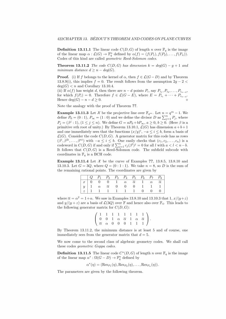
422CHAPTER 13. BEZOUT’S THEOREM AND CODES ON PLANE CURVES
Definition 13.11.1 The linear code C(D,G) of length n over Fq is the imageof the linear map α : L(G) → Fnq defined by α(f) = (f(P1), f(P2), . . . , f(Pn)).Codes of this kind are called geometric Reed-Solomon codes.
Theorem 13.11.2 The code C(D,G) has dimension k = deg(G) − g + 1 andminimum distance d ≥ n− deg(G).
Proof. (i) If f belongs to the kernel of α, then f ∈ L(G−D) and by Theorem13.8.9(i), this implies f = 0. The result follows from the assumption 2g − 2 <deg(G) < n and Corollary 13.10.4.(ii) If α(f) has weight d, then there are n− d points Pi, say Pi1 , Pi2 , . . . , Pin−d
,for which f(Pi) = 0. Therefore f ∈ L(G − E), where E = Pi1 + · · · + Pin−d
.Hence deg(G)− n− d ≥ 0. Note the analogy with the proof of Theorem ??.
Example 13.11.3 Let X be the projective line over Fqm . Let n = qm − 1. Wedefine P0 = (0 : 1), P∞ = (1 : 0) and we define the divisor D as
∑nj=1 Pj , where
Pj = (βj : 1), (1 ≤ j ≤ n). We define G = aP0 +bP∞, a ≥ 0, b ≥ 0. (Here β is aprimitive nth root of unity.) By Theorem 13.10.1, L(G) has dimension a+ b+ 1and one immediately sees that the functions (x/y)i, −a ≤ i ≤ b, form a basis ofL(G). Consider the code C(D,G). A generator matrix for this code has as rows(βi, β2i, . . . , βni) with −a ≤ i ≤ b. One easily checks that (c1, c2, . . . , cn) is acodeword in C(D,G) if and only if
∑nj=1 cj(β
l)j = 0 for all l with a < l < n−b.It follows that C(D,G) is a Reed-Solomon code. The subfield subcode withcoordinates in Fq is a BCH code.
Example 13.11.4 Let X be the curve of Examples ??, 13.8.5, 13.8.10 and13.10.3. Let G = 3Q, where Q = (0 : 1 : 1). We take n = 8, so D is the sum ofthe remaining rational points. The coordinates are given by
Q P1 P2 P3 P4 P5 P6 P7 P8
x 0 0 0 1 α α 1 α αy 1 α α 0 0 0 1 1 1z 1 1 1 1 1 1 0 0 0
where α = α2 = 1+α. We saw in Examples 13.8.10 and 13.10.3 that 1, x/(y+z)and y/(y+ z) are a basis of L(3Q) over F and hence also over F4. This leads tothe following generator matrix for C(D,G): 1 1 1 1 1 1 1 1
0 0 1 α α 1 α αα α 0 0 0 1 1 1
.
By Theorem 13.11.2, the minimum distance is at least 5 and of course, oneimmediately sees from the generator matrix that d = 5.
We now come to the second class of algebraic geometry codes. We shall callthese codes geometric Goppa codes.
Definition 13.11.5 The linear code C∗(D,G) of length n over Fq is the imageof the linear map α∗ : Ω(G−D)→ Fnq defined by
α∗(η) = (ResP1(η),ResP2
(η), . . . ,ResPn(η)).
The parameters are given by the following theorem.
13.11. CODES FROM ALGEBRAIC CURVES 423
Theorem 13.11.6 The code C∗(D,G) has dimension k∗ = n− deg(G) + g− 1and minimum distance d∗ ≥ deg(G)− 2g + 2.
Proof. Just as in Theorem 13.11.2, these assertions are direct consequencesof Theorem 13.10.1 (Riemann-Roch), using Theorem 13.10.8 (making the con-nection between the dimension of Ω(G) and l(W − G)) and Corollary 13.10.2(stating that the degree of a canonical divisor is 2g − 2).
Example 13.11.7 Let L = α1, . . . , αn be a set of n distinct elements of Fqm .Let g be a polynomial in Fqm [X] which is not zero at αi for all i. The (classical)Goppa code Γ(L, g) is defined by
Γ(L, g) = c ∈ Fnq |∑ ci
X − αi≡ 0 (mod g ).
Let Pi = (αi : 1), Q = (1 : 0) and D = P1 + · · · + Pn. If we take for E thedivisor of zeros of g on the projective line, then Γ(L, g) = C∗(D,E −Q) and
c ∈ Γ(L, g) if and only if∑ ci
X − αidX ∈ Ω(E −Q−D).
This is the reason that some authors extend the definiton of geometric Goppacodes to subfield subcodes of codes of the form C∗(D,G).It is a well-known fact that the parity check matrix of the Goppa code Γ(L, g)is equal to the following generator matrix of a generalized RS code
g(α1)−1 . . . g(αn)−1
α1g(α1)−1 . . . αng(αn)−1
... · · ·...
αr−11 g(α1)−1 . . . αr−1
n g(αn)−1
,
where r is the degree of the Goppa polynomial g. So Γ(L, g) is the subfieldsubcode of the dual of a generalized RS code. This is a special case of thefollowing theorem.
Theorem 13.11.8 The codes C(D,G) and C∗(D,G) are dual codes.
Proof. From Theorem 13.11.2 and Theorem 13.11.6 we know that k+ k∗ = n.So it suffices to take a word from each code and show that the inner product ofthe two words is 0. Let f ∈ L(G), η ∈ Ω(G −D). By Definitions 13.11.1 and13.11.5, the differential fη has no poles except possibly poles of order 1 in thepoints P1, P2, . . . , Pn. The residue of fη in Pi is equal to f(Pi)ResPi
(η). ByTheorem 13.9.16, the sum of the residues of fη over all the poles, that is to say,over the points Pi, is equal to zero. Hence we have
0 =
n∑i=1
f(Pi)ResPi(η) = 〈α(f), α∗(η)〉.
Several authors prefer the codes C∗(D,G) over geometric RS codes but thenonexperts in algebraic geometry probably feel more at home with polynomialsthan with differentials. That this is possible without loss of generality is statedin the following theorem.
424CHAPTER 13. BEZOUT’S THEOREM AND CODES ON PLANE CURVES
Theorem 13.11.9 Let X be a curve defined over Fq. Let P1, . . . , Pn be n ra-tional points on X . Let D = P1 + · · ·+Pn. Then there exists a differential formω with simple poles at the Pi such that ResPi
(ω) = 1 for all i. Furthermore
C∗(D,G) = C(D,W +D −G)
for all divisors G that have a support disjoint from the support of D, where Wis the divisor of ω.
So one can do without differentials and the codes C∗(D,G). However, it isuseful to have both classes when treating decoding methods. These use paritychecks, so one needs a generator matrix for the dual code.
In the next paragraph we treat several examples of algebraic geometry codes.It is already clear that we find some good codes. For example from Theorem13.11.2 we see that such codes over a curve of genus 0 (the projective line) areMDS codes. In fact, Theorem 13.11.2 says that d ≥ n − k + 1 − g, so if g issmall, we are close to the Singleton bound.
13.12 Rational functions and divisors on planecurves
This section will be finished together with the correction of Section 7.
rational cycles, Frobenius, divisors..... rational functions discrete valuation,discrete valuation ring.
Example 13.12.1 Consider the curve X with homogeneous equation
XaY c + Y b+cZa−b +XdZa+c−d = 0
with d < b < a as in Example 13.3.10. The divisor of the rational function x/zis (x
z
)= (X · L)− (X · N ) = (b+ c)P − bQ− cR.
The divisor of the rational function y/z is(yz
)= (X ·M)− (X · N ) = dP − aQ− (a− d)R.
Hence the divisor of (x/z)α(y/z)β is
((b+ c)α+ dβ)P + (−bα− aβ)Q+ (−cα+ (a− d)β)R.
It has only a pole at Q if and only if cα ≤ (a − d)β. (This will serve as amotivation for the choice of the basis of R in Proposition ??.)
13.13 Resolution or normalization of curves
13.14 Newton polygon of plane curves
[?]
13.15. NOTES 425
13.15 Notes
Goppa submitted his seminal paper [?] in June 1975 and it was published in1977. Goppa also published three more papers in the eighties [?, ?, ?] and abook [?] in 1991.Most of this section is standard textbook material. See for instance [?, ?, ?, ?]to mention a few. Section 13.4 is a special case of Goppa’s construction andcomes from [?]. The Hermitian curves in Example 13.2.4 and their codes havebeen studied by many authors. See [?, ?, ?, ?]. The Klein curve goes back to F.Klein [?] and has been studied thoroughly, also over finite fields in connectionwith codes. See [?, ?, ?, ?, ?, ?, ?, ?].

426CHAPTER 13. BEZOUT’S THEOREM AND CODES ON PLANE CURVES

Chapter 14
Curves
Ruud Pellikaan
427
428 CHAPTER 14. CURVES
14.1 Algebraic varieties
14.2 Curves
14.3 Curves and function fields
14.4 Normal rational curves and Segre’s prob-lems
14.5 The number of rational points
14.5.1 Zeta function
14.5.2 Hasse-Weil bound
14.5.3 Serre’s bound
14.5.4 Ihara’s bound
14.5.5 Drinfeld-Vladut bound
14.5.6 Explicit formulas
14.5.7 Oesterle’s bound
14.6 Trace codes and curves
14.7 Good curves
14.7.1 Maximal curves
14.7.2 Shimura modular curves
14.7.3 Drinfeld modular curves
14.7.4 Tsfasman-Vladut-Zink bound
14.7.5 Towers of Garcia-Stichtenoth
14.8. APPLICATIONS OF AG CODES 429
14.8 Applications of AG codes
14.8.1 McEliece crypto system with AG codes
14.8.2 Authentication codes
Here we consider an application of AG-codes to authentication. Recall that inChapter 10, Section 10.3.1 we started to consider authentication codes that areconstructed via almost universal and almost strongly universal hash functions.They, in turn, can be constructed using error-correction codes. We recall twomethods of constructing authentication codes (almost strongly universal hashfunction to be precise) from error-correcting codes:
1. Construct AU-families from codes as per Proposition 10.3.7 and then useStinson’s composition method, Theorem 10.3.10.
2. Construct ASU-families directly from error-correcting codes.
As an example we mentioned ASU-families constructed as in (1.) using Reed-Solomon codes, Exercise 10.3.2. Now we would like to move on and present ageneral construction of almost universal hash functions that employs AG-codes.The following proposition formulates the result we need.
Proposition 14.8.1 Let C be an algebraic curve over Fq with N + 1 rationalpoints P0, P1, . . . , PN . Fix P = Pi for some i = 0, . . . , N and let WS(P ) =0, w1, w2, . . . be the Weierstraß semigroup of P . Then for each j ≥ 1 one canconstruct an almost universal hash family ε− U(N, qj , q), where ε ≤ wj/N .
Proof. Indeed, construct an AG-code C = CL(D,wjP ), where the divisorD is defined as D =
∑k 6=i Pk and P = Pi. So C is obtained as an image of
the evaluation map for the functions that have a pole only at P and its order isbounded by wj . From ?? we have that length of C is N , dimC = dimL(wjP ) =j, and d(C) ≥ N − deg(wjP ) = N − wj . So 1 − d(C)/N ≤ wj and now theclaim easily follows.
As an example of this proposition, we show next how one can obtain AU-familiesfrom Hermitian curves.
Proposition 14.8.2 For every prime power q and every i ≤ q, Hermitian curveyq + y = xq+1 over Fq2 yields
i
q2− U(q3, qi
2+i, q2).
Proof. Recall from ?? that Hermitian curve over Fq2 has q3 + 1 rationalpoints P1, . . . , Pq3 , P∞. Construct C = CL(D,wiP ), where P = P∞ is a place
at infinity, D =∑q3
i=1 Pi, and WS(P ) = 0, w1, w2, . . . . It is known that theWeierstraß semigroup WS(P ) is generated by q and q + 1.Let us show that w(i+1
2 ) = iq for all i ≤ q. We proceed by induction. For i = 1
we have w1 = q, which is obviously true. Then suppose that for some i ≥ 1 wehave w(i
2)= (i− 1)q and want to prove w(i+1
2 ) = iq. Clearly, for this we need to
show that there is exactly i−1 non-gaps between (i−1)q and iq (these numbersthemselves are not included in the count). So for the non-gaps aq + b(q + 1)
430 CHAPTER 14. CURVES
that lie between (i − 1)q and iq we have: (i − 1)q < aq + b(q + 1) < iq. Thus,automatically, a < i. We have then
(i− a− 1)q
q + 1< b < (i− a)
q
q + 1. (14.1)
So from here we see that 0 < a < i−1, because for a = i−1 we have b < q/(q+1),which is not possible. So there are i− 1 values of a, namely 0, . . . , i− 2, whichcould give rise to a non-gap. The interval from (14.1) has length q/(q + 1) < 1.So it may contain at most one integer. If i−a < q+1, then (i−a−1)q/(q+1) <i − a − 1 < (i − a)q/(q + 1). And thus an integer i − a − 1 is always in thatinterval if i − a < q + 1. But for 0 < a < i − 1, the condition i − a < q + 1 isalways full filled, since i ≤ q by the assumption. Thus for every 0 < a < i− 1,there exists exactly one b = i−a−1, such that aq+b(q+1) lies between (i−1)qand iq. It is also easily seen that all these non-gaps are different. So, indeed,w(i+1
2 ) = iq for all i ≤ q.Now the claim follows form Proposition 14.8.1.
As a consequence we have
Corollary 14.8.3 Let a, b be positive integers such that b ≤ a ≤ 2b and qa is asquare. Then there exists
2
qb− SU(q5a/2+b, qaq
2(a−b)/2, qb).
Proof. Do the ”Hermitian” construction from the previous proposition overFqa and i = qa−b. Then the claim follows from Theorem 10.3.10 and Exercise10.3.2.
*** Suzuki curves? ***To get some feeling about all these, the reader is advised to solve Exercise 14.8.1.Now we move to (2.). We would like to show the direct construction of Xing et.al ?? that uses AG-codes.
Theorem 14.8.4 Let C be an algebraic curve over Fq of genus g and let R besome set of rational points of C. Let G be a positive divisor such that |R| >deg(G) ≥ 2g + 1 and R ∩ supp(G) = ∅. Then there exists ε − ASU(N,n,m)with N = q|R|, n = qdeg(G)−g+1,m = q, and ε = deg(G)/|R|.
Proof. Consider the set H = h(P,α) : L(G) → Fq|h(P,α)(f) = f(P ) +α, f ∈ L(G). Take H as functions in the definition of an ASU-family; setX = L(G), Y = Fq. Then |X| = dimL(G) = deg(G)− g+ 1, because deg(G) ≥2g + 1 > 2g − 1.It can be shown (see Exercise 14.8.2) that if deg(G) ≥ 2g + 1, then |H| = q|R|.It is also easy to see that for any a ∈ L(G) and any b ∈ Fq there exists exactly|R| = |H|/q functions from H that map a to b. This proves the first part ofbeing ASU. As to the second part consider
m = maxa1 6=a2∈L(G);b1,b2∈Fq
|h(P,α) ∈ H|h(P,α)(a1) = b1;h(P,α)(a2) = b2| =
= maxa1 6=a2∈L(G);b1,b2∈Fq
|(P, α) ∈ R× Fq|(a1 − a2 − b1 + b2)(P ) = 0; a2(P ) + α = b2|.
14.9. NOTES 431
As a1−a2 ∈ L(G)\0 and b1−b2 ∈ Fq we see that a1−a2−b1+b2 ∈ L(G)\0.Note that there cannot be more than deg(G) zeros of a1 − a2 − b1 + b2 amongpoints in R (cf. ??). Since α in (P, α) is uniquely determined by P ∈ R,we see that there are at most deg(G) pairs (P, α) ∈ R × Fq that satisfy both(a1 − a2 − b1 + b2)(P ) = 0, a2(P ) + α = b2. In other words,
m ≤ deg(G) =deg(G) · |H||R| · q
.
We can take now ε = deg(G)/|R| in Definition 10.3.8.
Again we present here a concrete result coming from Hermitian codes.
Corollary 14.8.5 Let q be a prime power and let an integer q3 > d ≥ q(q−1)+1be given. Then there exists
d
q3−ASU(q5, qd−q(q−1)/2+1, q2).
Proof. Consider again the Hermitian curve over Fq2 . Take any rationalpoint P and construct C = CL(D,G), where D =
∑P ′ 6=P P
′ is the sum of all
remaining rational points (there is q3 of them), and G = dP . Then the claimfollows directly from the previous theorem.
For a numerical example we refer again to Exercise 14.8.1.
14.8.3 Fast multiplication in finite fields
14.8.4 Correlation sequences and pseudo random sequences
14.8.5 Quantum codes
14.8.6 Exercises
14.8.1 Suppose we would like to obtain an authentication code with PS =2−20 ≥ PI and log |S| ≥ 234. Give the parameters of such an authenticationcode using the following constructions. Compare the results.
• OA-construction as per Theorem 10.3.5.
• RS-construction as per Exercise 10.3.2.
• Hermitian construction as per Corollary 14.8.3.
• Hermitian construction as per Corollary 14.8.5.
14.8.2 Let H = h(P,α) : L(G) → Fq|h(P,α)(f) = f(P ) + α, f ∈ L(G) as inthe proof of Theorem 14.8.4. Prove that if deg(G) ≥ 2g + 1, then |H| = q|R|.
14.9 Notes

432 CHAPTER 14. CURVES
Bibliography
[1]
[2]
[3] N. Abramson. Information theory and coding. McGraw-Hill, New York,1963.
[4] A.V. Aho, J.E. Hopcroft, and J.D. Ulman. The design and analysis ofcomputer algorithms. Addison-Wesley, Reading, 1979.
[5] M. Aigner. Combinatorial theory. Springer, New York, 1979.
[6] A. Ashikhmin and A. Barg. Minimal vectors in linear codes. IEEE Trans-actions on Information Theory, 44(5):2010–2017, 1998.
[7] C.A. Athanasiadis. Characteristic polynomials of subspace arrangementsand finite fields. Advances in Mathematics, 122:193–233, 1996.
[8] A. Barg. The matroid of supports of a linear code. AAECC, 8:165–172,1997.
[9] A. Barg. Complexity issues in coding theory. In V.S. Pless and W.C.Huffman, editors, Handbook of coding theory, volume 1, pages 649–754.North-Holland, Amsterdam, 1998.
[10] E.R. Berlekamp. Key papers in the development of coding theory. IEEEPress, New York, 1974.
[11] E.R. Berlekamp. Algebraic coding theory. Aegon Park Press, Laguna Hills,1984.
[12] D.J. Bernstein, J. Buchmann, and E. Dahmen, editors. Post-QuantumCryptography. Springer-Verlag, Berlin Heidelberg, 2009.
[13] J. Bierbrauer, T. Johansson, G. Kabatianskii, and B. Smeets. On familiesof hash functions via geometric codes and concatenation. In Advances inCryptology – CRYPTO ’93. Lecture Notes in Computer Science, volume773, pages 331–342, 1994.
[14] N. Biggs. Algebraic graph theory. Cambridge University Press, Cambridge,1993.
433
434 BIBLIOGRAPHY
[15] E. Biham and A. Shamir. Differential cryptanalysis of DES-like cryp-tosystems. In Advances in Cryptology – CRYPTO ’90. Lecture Notes inComputer Science, volume 537, pages 2–21, 1990.
[16] G. Birkhoff. On the number of ways of coloring a map. Proc. EdinburghMath. Soc., 2:83–91, 1930.
[17] A. Bjorner and T. Ekedahl. Subarrangments over finite fields: Chomo-logical and enumerative aspects. Advances in Mathematics, 129:159–187,1997.
[18] J.E. Blackburn, N.H. Crapo, and D.A. Higgs. A catalogue of combinatorialgeometries. Math. Comp., 27:155–166, 1973.
[19] R.E. Blahut. Theory and practice of error control codes. Addison-Wesley,Reading, 1983.
[20] R.E. Blahut. Algebraic codes for data transmission. Cambridge UniversityPress, Cambridge, 2003.
[21] I.F. Blake. Algebraic coding theory: History and development. Dowden,Hutchinson and Ross, Stroudsburg, 1973.
[22] G.R. Blakely. Safeguarding cryptographic keys. In Proceedings of 1979national Computer Conf., pages 313–317, New York, 1979.
[23] G.R. Blakely and C. Meadows. Security of ramp schemes. In Advances inCryptology – CRYPTO ’84. Lecture Notes in Computer Science, volume196, pages 242–268, 1985.
[24] A. Blass and B.E. Sagan. Mobius functions of lattices. Advances in Math-ematics, 129:94–123, 1997.
[25] T. Britz. MacWilliams identities and matroid polynomials. The ElectronicJournal of Combinatorics, 9:R19, 2002.
[26] T. Britz. Relations, matroids and codes. PhD thesis, Univ. Aarhus, 2002.
[27] T. Britz. Extensions of the critical theorem. Discrete Mathematics,305:55–73, 2005.
[28] T. Britz. Higher support matroids. Discrete Mathematics, 307:2300–2308,2007.
[29] T. Britz and C.G. Rutherford. Covering radii are not matroid invariants.Discrete Mathematics, 296:117–120, 2005.
[30] T. Britz and K. Shiromoto. A macwillimas type identity for matroids.Discrete Mathematics, 308:4551–4559, 2008.
[31] T. Brylawski. A decomposition for combinatorial geometries. Transactionsof the American Mathematical Society, 171:235–282, 1972.
[32] T. Brylawski and J. Oxley. Intersection theory for embeddings of matroidsinto uniform geometries. Stud. Appl. math., 61:211–244, 1979.
BIBLIOGRAPHY 435
[33] T. Brylawski and J. Oxley. Several identities for the characteristic polyno-mial of a combinatorial geometry. Discrete Mathematics, 31(2):161–170,1980.
[34] T.H. Brylawski and J.G. Oxley. The tutte polynomial and its applications.In N. White, editor, Matroid Applications. Cambridge University Press,Cambridge, 1992.
[35] J. Buchmann. Introduction to Cryptography. Springer, Berlin, 2004.
[36] J.P. Buhler, H.W. Lenstra Jr., and C. Pomerance. Factoring integers withthe number field sieve. In A.K. Lenstra and H.W. Lenstra Jr., editors,The development of the number field sieve. Lecture Notes in ComputerScience, volume 1554, pages 50–94. Springer, Berlin, 1993.
[37] L. Carlitz. The arithmetic of polynomials in a galois field. AmericanJournal of Mathematics, 54:39–50, 1932.
[38] P. Cartier. Les arrangements d’hyperplans: un chapitre de geometriecombinatoire. Seminaire N. Bourbaki, 561:1–22, 1981.
[39] H. Chen and R. Cramer. Algebraic geometric secret sharing schemes andsecure multi-party computations over small fields. In C. Dwork, editor,Advances in Cryptology – CRYPTO 2006. Lecture Notes in ComputerScience, volume 4117, pages 521–536. Springer, Berlin, 2006.
[40] C. Cid and H. Gilbert. AES security report,ECRYPT, IST-2002-507932. Available online athttp://www.ecrypt.eu.org/ecrypt1/documents/D.STVL.2-1.0.pdf.
[41] H. Cohen and G. Frey. Handbook of elliptic and hyperelliptic curve cryp-tography. CRC Press, Boca Raton, 2006.
[42] H. Crapo. Mobius inversion in lattices. Archiv der Mathematik, 19:595–607, 1968.
[43] H. Crapo. The tutte polynomial. Aequationes Math., 3:211–229, 1969.
[44] H. Crapo and G.-C. Rota. On the foundations of combinatorial theory:Combinatorial geometries. MIT Press, Cambridge MA, 1970.
[45] J. Daemen and R. Vincent. The design of rijndael. Springer, Berlin, 1992.
[46] J. Daemen and R. Vincent. The wide trail design strategy. In B. Honary,editor, Cryptography and Coding 2001. Lecture Notes in Computer Sci-ence, volume 2260, pages 222–238. Springer, Berlin, 2001.
[47] W. Diffie. The first ten years of public key cryptography. In J. Simmons,editor, Contemporary Cryptology: The Science of Information Integrity,pages 135–176. IEEE Press, Piscataway, 1992.
[48] W. Diffie and M.E. Hellman. New directions in cryptography. IEEE Trans.Inform. Theory, 22:644–654, 1976.
436 BIBLIOGRAPHY
[49] J. Ding, J.E. Gower, and D.S. Schmidt. Multivariate Public Key Cryp-tosystems. Advances in Information Security. Springer Science+BusinessMedia, LLC, 2006.
[50] J.L. Dornstetter. On the equivalence of the Berlekamp-Massey and theEuclidean algorithms. IEEE Trans. Inform. Theory, 33:428–431, 1987.
[51] W.M.B. Dukes. On the number of matroids on a finite set. SeminaireLotharingien de Combinatoire, 51, 2004.
[52] I. Duursma. Algebraic geometry codes: general theory. In D. RuanoE. Martinez-Moro, C. Munuera, editor, Advances in algebraic geometrycodes, pages 1–48. World Scientific, New Jersey, 2008.
[53] I.M. Duursma. Decoding codes from curves and cyclic codes. PhD thesis,Eindhoven University of Technology, 1993.
[54] I.M. Duursma and R. Kotter. Error-locating pairs for cyclic codes. IEEETrans. Inform. Theory, 40:1108–1121, 1994.
[55] T. ElGamal. A public key cryptosystem and a signature scheme based ondiscrete logarithms. IEEE Trans. Inform. Theory, 31:469–472, 1985.
[56] G. Etienne and M. Las Vergnas. Computing the Tutte polynomial of ahyperplane arrangement. Advances in Applied Mathematics, 32:198–211,2004.
[57] L. Euler. Solutio problematis ad geometriam situs pertinentis. Commen-tarii Academiae Scientiarum Imperialis Petropolitanae, 8:128–140, 1736.
[58] E.N. Gilbert, F.J. MacWilliams, and N.J.A. Sloan. Codes, which detectdeception. Bell Sys. Tech. J., 33(3):405–424, 1974.
[59] C. Greene. Weight enumeration and the geometry of linear codes. Studiesin Applied Mathematics, 55:119–128, 1976.
[60] C. Greene and T. Zaslavsky. On the interpretation of whitney numbersthrough arrangements of hyperplanes, zonotopes, non-radon partitionsand orientations of graphs. Trans. Amer. Math. Soc., 280:97–126, 1983.
[61] R.W. Hamming. Error detecting and error correcting codes. Bell SystemTechn. Journal, 29:147–160, 1950.
[62] R.W. Hamming. Coding and Information Theory. Prentice-Hall, NewJersey, 1980.
[63] T. Helleseth, T. Kløve, and J. Mykkeltveit. The weight distribution ofirreducible cyclic codes with block lengths n1((ql− 1)/n). Discrete Math-ematics, 18:179–211, 1977.
[64] M. Hermelina and K. Nyberg. Correlation properties of the bluetooth com-biner generator. In Dan Boneh, editor, Information Security and Cryptol-ogy ICISC 1999. Lecture Notes in Computer Science, volume 1787, pages17–29. Springer, Berlin, 2000.
BIBLIOGRAPHY 437
[65] A.E. Heytmann and J.M. Jensen. On the equivalence of the Berlekamp-Massey and the Euclidean algorithm for decoding. IEEE Trans. Inform.Theory, 46:2614–2624, 2000.
[66] L.J. Hoffman. Modern methods for computer security and privacy.Prentice-Hall, New Jersey, 1977.
[67] W.C. Huffman and V.S. Pless. Fundamentals of error-correcting codes.Cambridge University Press, Cambridge, 2003.
[68] R.P.M.J. Jurrius. Classifying polynomials of linear codes. Master’s thesis,Leiden University, 2008.
[69] J. Justesen. On the complexity of decoding Reed-Solomon codes. IEEETrans. Inform. Theory, 22:237–238, 1976.
[70] E.D. Karnin, J.W. Greene, and M.E. Hellman. On secret sharing systems.IEEE Trans. Inform. Theory, 29(1):35–31, 1983.
[71] T. Kløve. The weight distribution of linear codes over GF(ql) havinggenerator matrix over GF(q). Discrete Mathematics, 23:159–168, 1978.
[72] T. Kløve. Support weight distribution of linear codes. Discrete Matemat-ics, 106/107:311–316, 1992.
[73] D.E. Knuth. The asymptotic number of geometries. J. Comb. Theory Ser.A, 16:398–400, 1974.
[74] R. Lidl and H. Niederreiter. Introduction to finite fields and their appli-cations. Cambridge University Press, Cambridge, 1994.
[75] S. Lin and D.J. Costello. Error control coding : fundamentals and appli-cations. Prentice-Hall, New Jersey, 1983.
[76] J.H. van Lint. Mathematics and the compact disc. Nieuw Archief voorWiskunde, 16:183–190, 1998.
[77] David MacKay. Information theory, inference and learning algorithms.Cambridge University Press, Cambridge, 2003.
[78] F.J. MacWilliams and N.J.A. Sloane. The theory of error-correcting codes.Elsevier Sc. Publ., New York, 1977.
[79] J.L. Massey. Shift-register synthesis and BCH decoding. IEEE Trans.Inform. Theory, 15:122–127, 1969.
[80] J.L. Massey. Minimal codewords and secret sharing. In In Proc. SixthJoint Swedish-Russian Workshop on Information theory, Molle, Sweden,pages 276–279, 1993.
[81] J.L. Massey. On some applications of coding theory. In Cryptography,Codes and Ciphers: Cryptography and Coding IV, pages 33–47. 1995.
[82] M. Matsui. Linear cryptanalysis method for DES cipher. In T. Helleseth,editor, Advances in Cryptology - EUROCRYPT 1993. Lecture Notes inComputer Science, volume 765, pages 386–397. Springer, Berlin, 1994.
438 BIBLIOGRAPHY
[83] K.S. McCurley. A key distribution system equivalent to factoring. Journalof Cryptology, 1:95–105, 1988.
[84] R.J. McEliece. The theory of information and coding. Addison-WesleyPubl. Comp., Reading, 1977.
[85] R.J. McEliece and D.V. Sawate. On sharing secrets and Reed-Solomoncodes. Communications of ACM, 24:583–584, 1981.
[86] R.J. McEliece and L. Swanson. Reed-Solomon codes and the explorationof the solar system. In S.B. Wicker and V.K. Bhargava, editors, Reed-Solomon codes and their applications, pages 25–40. IEEE Press, New York,1994.
[87] A. Menezes, P. van Oorschot, and S. Vanstone. Handbook of ap-plied cryptography. CRC Press, Boca Raton, 1996. Available onlinehttp://www.cacr.math.uwaterloo.ca/hac/.
[88] C.J. Mitchell, F. Piper, and P. Wild. Digital signatures. In J. Simmons,editor, Contemporary Cryptology: The Science of Information Integrity,pages 325–378. IEEE Press, New York, 1992.
[89] J. Nechvatal. Public key cryptography. In J. Simmons, editor, Contem-porary Cryptology: The Science of Information Integrity, pages 177–288.IEEE Press, New York, 1992.
[90] National Institute of Standards and Technology. Data encryp-tion standard (DES). Federal Information Processing Stan-dards Publication, National Technical Information Service,Springfield, VA, Apr., reaffirmed version available online athttp://csrc.nist.gov/publications/fips/fips46-3/fips46-3.pdf,46(3), 1977.
[91] National Institute of Standards and Technology. Advanced en-cryption standard (AES). Federal Information Standards Publicationhttp://www.csrc.nist.gov/publications/fips/fips197/fips-197.pdf,197(26), 2001.
[92] P. Orlik and H. Terao. Arrangements of hyperplanes, volume 300.Springer-Verlag, Berlin, 1992.
[93] W.W. Peterson and E.J. Weldon. Error-correcting codes. MIT Pres, Cam-bridge, 1972.
[94] J. Pieprzyk and X.M. Zhang. Ideal threshold schemes from mds codes. InG. Goos, J. Hartmanis, and J. van Leeuwen, editors, Information Securityand Cryptology ICISC 2002. Lecture Notes in Computer Science, volume2587, pages 269–279. Springer, Berlin, 2003.
[95] V.S. Pless and W.C. Huffman. Handbook of coding theory. Elsevier Sc.Publ., New York, 1998.
[96] C. Pomerance. Factoring. In C. Pomerance, editor, Cryptology and Com-putational Number Theory, volume 42, pages 27–47. American Mathemat-ical Society, Rhode Island, 1990.
BIBLIOGRAPHY 439
[97] M. Rabin. Digitalized signatures and public-key functions as intractableas factorization. MIT/LCS/TR-212, 1979.
[98] C.T. Retter. Bounds on Goppa codes. IEEE Trans. Inform. Theory,22(4):476–482, 1976.
[99] T. Richardson and R. Urbanke. Modern coding theory. Cambridge Uni-versity Press, Cambridge, 2008.
[100] R.L. Rivest, A. Shamir, and L.M. Adleman. A method for obtaining dig-ital signatures and public-key cryptosystems. Communications of ACM,21:120–126, 1977.
[101] G.-C. Rota. On the foundations of combinatorial theory I: Theory ofmobius functions. Zeit. fur Wahrsch., 2:340–368, 1964.
[102] R.A. Rueppel. Analysis and Design of Stream Ciphers. Springer-Verlag,Berlin, 1986.
[103] R. Safavi-Naini, H. Wang, and C. Xing. Linear authentication codes:Bounds and constructions. In C. Pandu Rangan and C. Ding, editors,Advances in Cryptology - INDOCRYPT 2001. Lecture Notes in ComputerScience, volume 2247, pages 127–135. Springer, Berlin, 2001.
[104] D. Sarwate. On the complexity of decoding Goppa codes. IEEE Trans.Inform. Theory, 23:515–516, 1977.
[105] K.A. Schouhamer Immink. Reed-Solomon codes and the compact disc. InS.B. Wicker and V.K. Bhargava, editors, Reed-Solomon codes and theirapplications, pages 41–59. IEEE Press, New York, 1994.
[106] A. Shamir. How to share a secret. Communications of ACM, 22:612–613,1979.
[107] A. Shannon. A mathematical theory of communication. Bell Syst. echn.Journal, 27:379–423, 623–656, 1948.
[108] P. Shor. Polynomial time algorithms for prime factorization and discretelogarithms on a quantum computer. SIAM Journal of Computing, 26:1484.
[109] J. Simonis. The effective length of subcodes. AAECC, 5:371–377, 1993.
[110] A.N. Skorobogatov. Linear codes, strata of grassmannians, and the prob-lems of segre. In H. Stichtenoth and M.A. Tfsafsman, editors, CodingTheory and Algebraic Geometry, Lecture Notes Math. vol 1518, pages 210–223. Springer-Verlag, Berlin, 1992.
[111] D. Slepian. Key papers in the development of information theory. IEEEPress, New York, 1974.
[112] M.E. Smid and D.K. Branstad. The data encryption standard: Past andfuture. In J. Simmons, editor, Contemporary Cryptology: The Science ofInformation Integrity, pages 43–64. IEEE Press, New York, 1992.
[113] R.P. Stanley. Enumerative combinatorics, vol. 1. Cambridge UniversityPress, Cambridge, 1997.
440 BIBLIOGRAPHY
[114] R.P. Stanley. An introduction to hyperplane arrangements. In Geomet-ric combinatorics, IAS/Park City Math. Ser., 13, pages 389–496. Amer.Math. Soc., Providence, RI, 2007.
[115] D.R. Stinson. The combinatorics of authentication and secrecy. Journalof Cryptology, 2:23–49, 1990.
[116] D.R. Stinson. Combinatorial characterization of authentication codes.Designs, Codes and Cryptography, 2:175–187, 1992.
[117] D.R. Stinson. Cryptography, theory and practice. CRC Press, Boca Raton,1995.
[118] Y. Sugiyama, M. Kasahara, S. Hirasawa, and T. Namekawa. A methodfor solving the key equation for decoding Goppa codes. Information andControl, 27:87–99, 1975.
[119] W.T. Tutte. A ring in graph theory. Proc. Cambridge Philos. Soc., 43:26–40, 1947.
[120] W.T. Tutte. An algebraic theory of graphs. PhD thesis, Univ. Cambridge,1948.
[121] W.T. Tutte. A contribution to the theory of chromatic polynomials. Cana-dian Journal of Mathematics, 6:80–91, 1954.
[122] W.T. Tutte. Matroids and graphs. Transactions of the American Mathe-matical Society, 90:527–552, 1959.
[123] W.T. Tutte. Lectures on matroids. J. Res. Natl. Bur. Standards, Sect. B,69:1–47, 1965.
[124] W.T. Tutte. On the algebraic theory of graph coloring. J. Comb. Theory,1:15–50, 1966.
[125] W.T. Tutte. On dichromatic polynomials. J. Comb. Theory, 2:301–320,1967.
[126] W.T. Tutte. Cochromatic graphs. J. Comb. Theory, 16:168–174, 1974.
[127] W.T. Tutte. Graphs-polynomials. Advences in Applied Mathematics,32:5–9, 2004.
[128] J.H. van Lint and R. M. Wilson. A course in combinatorics. CambridgeUniversity Press, Cambridge, 1992.
[129] H. Whitney. The colorings of graphs. Ann. Math., 33:688–718, 1932.
[130] H. Whitney. A logical expansion in mathematics. Bull. Amer. Math. Soc.,38:572–579, 1932.
[131] H. Whitney. On the abstract properties of linear dependence. Amer. J.Math., 57:509–533, 1935.
[132] G. Whittle. A charactrization of the matroids representable over gf(3)and the rationals. J. Comb. Theory Ser. B, 65(2):222–261, 1995.
BIBLIOGRAPHY 441
[133] G. Whittle. On matroids representable over gf(3) and other fields. Trans.Amer. Math. Soc., 349(2):579–603, 1997.
[134] S.B. Wicker. Deep space applications. In V.S. Pless and W.C. Huffman,editors, Handbook of coding theory, volume 2, pages 2119–2169. North-Holland, Amsterdam, 1998.
[135] S.B. Wicker and V.K. Bhargava. Reed-Solomon codes and their applica-tions. IEEE Press, New York, 1994.
[136] R.J. Wilson and J.J. Watkins. Graphs; An introductory approach. J. Wiley& Sons, New York, 1990.
[137] A.C.-C. Yao. Protocols for secure computations. Extended Abstract, 23rdAnnual Symposium on Foundations of Computer Science, FOCS 1982,pages 160–164, 1982.
[138] J. Yuan and C. Ding. Secret sharing schemes from three classes of linearcodes. IEEE Trans. Inform. Theory, 52(1):206–212, 2006.
[139] T. Zaslavsky. Facing up to arrangements: Face-count fomulas for parti-tions of space by hyperplanes. Mem. Amer. Math. Soc. vol. 1, No. 154,Amer. Math. Soc., 1975.
[140] T. Zaslavsky. Signed graph colouring. Discrete. Math., 39:215–228, 1982.
Index
action, 40adjacent, 123Adleman, 311AES, 302algebra, 14algorithm
APGZ, 233basic, 273efficient, 35Euclidean, 191, 277Sudan, 286Sugiyama, 277
alphabet, 18anti-symmetric, 136arc, 95Arimoto, 233arrangement, 98
central, 98essential, 98graphic, 127simple, 98
arrayorthogonal, 159, 160
linear, 160atom, 141atomic, 141attack
adaptive chosen-ciphertext, 300adaptive chosen-plaintext, 300chosen-plaintext, 300ciphertext
chosen, 300ciphertext-only, 300known-plaintext, 300related-key, 300
authentication code, 318MAC, 317message, 317
automorphism, 41monomial, 42permutation, 42
axiomcircuit elimination, 130independence augmentation, 128
balanced, 84ball, 19basis, 22
external, 131internal, 131
Berlekamp, 334bilinear, 30binary cipher, 329binomial
Gaussian, 39, 93Bose, 214bound
AB, 223BCH, 214Bush, 161Gilbert, 72Gilbert-Varshamov, 73greatest lower, 139Griesmer, 68Hamming, 69HT, 220Johnson, 282least upper, 139Plotkin, 71Roos, 222shift, 225Singleton, 63sphere-covering, 70sphere-packing, 69Varshamov, 73
bound:redundancy, 74box
delay, 330S, 304
Brickell, 317bridge, 124broken
442
INDEX 443
partially, 300totally, 300
capacity, 14, 37error-correcting, 34, 282
chainextension of, 142maximal, 142of length, 137
channelbinary symmetric, 36q-ary symmetric, 36
character, 85principal, 85
characteristic, 201Chaudhuri, 214Chinese remainder, 207cipher
alphabetic substitution, 298block, 296Caesar, 296Feistel, 302iterative block, 302permutation, 297self-synchronizing stream, 330stream, 329substitution, 296, 298transposition , 297Vigenere, 298
ciphertext, 295, 296confusion, 298diffusion, 297
circuit, 130class
parallel, 91closed
algebraically, 202closure, 145cocircuit, 130code
alternant, 259augmented, 51BCH, 215
narrow sense, 215primitive, 215
block, 18Cauchy, 67
generalized, 67concatenated, 61constant weight, 72
convolutional, 18cycle, 127degenerate, 93dual, 30
complementary, 31self, 31weakly self, 31
error-correcting, 13expurgated, 52extended, 48extension by scalars, 104, 251Gallager, 127genus, 102geometric Goppa, 422Golay, 60
ternary, 32Goppa, 260graph, 127
sparse, 127Tanner, 127
Hamming, 22, 29hull, 31inner, 61lengthened, 52linear, 21low-density parity check, 127maximum distance separable, 64MDS, 64Melas, 228orthogonal, 30, 31
self, 31outer, 61projective, 94punctured, 47, 107reduced, 145Reed-Muller, 266Reed-Solomon, 241
extended, 243generalized, 66, 243geometric, 422
residual, 68restricted, 47restriction by scalars, 214, 251reverse, 196shortened, 50, 107simplex, 29sub, 22
even weight, 22subfield, 214, 251
super, 22, 214, 251
444 INDEX
trivial, 23Zetterberg, 228
codeword, 18minimal, 156nearest, 34
codimension, 92coding
source, 13color, 124combinatorics, 14comparable, 136complexity
data, 301implementation, 302linear, 334
componentconnected, 127
compressiondata, 13
computationsecure multi-party, 349
conjectureMDS, 104
connected, 126connection, 331consecutive, 216constant
S-box, 306constraints, 160construction
(a+ x|b+ x|a+ b− x), 58(u+ v|u− v), 57(u|u+ v), 56(u|v), 56
contractionmatroid, 133
coordinatehomogeneous, 91
coordinateshomogeneous
standard, 92correlation immune, 334coset, 35, 191
cyclotomic, 208coset leader, 35cover, 139Cramer, 234cryptanalysis
algebraic, 307cryptography
multivariate, 316cryptosystem, 295
asymmetric, 296, 309knapsack, 316public, 296RSA, 310, 311symmetric, 295
cycle, 126cyclic, 43, 189
Daemen, 302decision
hard, 16soft, 16
decoder, 34complete, 34coset leader, 35half the minimum distance, 34incomplete, 15list, 16, 35, 281minimum distance, 34nearest neighbor, 34
decodingcorrect, 34
decryption, 296El Gamal, 315McEliece, 337Niederreiter, 339RSA, 312
deletion, 149matroid, 133
Delsarte, 258demodulation, 16dependent, 128depth, 159derivation, 417derivative
formal, 202DES, 302
triple, 346detection
error, 26diagram
Hasse, 139, 142Diffie, 309, 316dimension, 21distance
bounded, 34designed minimum, 215Hamming, 18
INDEX 445
minimum, 19distribution
weight, 79division with rest, 191divisor, 415
canonical, 418degree, 415effective, 415greatest common, 191principal, 416support, 415
DLP, 310domain
Euclidean, 191dual, 30, 93
selfformally, 88quasi, 44
edge, 123acyclic, 124
El Gamal, 314Elias, 281elimination
Gaussian, 24embedded, 92encoder, 18
systematic, 25encoding, 23, 195encryption, 296
AES, 307confusion, 304DES, 304diffusion, 304El Gamal, 315McEliece, 337Niederreiter, 339RSA, 312
end, 123entropy function, 75enumerator
weight, 79average, 84coset leader, 35extended, 105generalized, 113homogeneous, 79
equalitymodular, 142
equation
Key, 236equivalent, 41
generalized, 42monomial, 42permutation, 42
error, 34decoding, 15, 34number of, 27, 34undetected, 89
Euclid, 191, 277EuclidSugiyama, 277Euler, 206evaluation, 243expand, 302explicit, 26, 91exponent
universal, 317
failuredecoding, 15, 34
familyalmost universal, 322
feedback, 331Feistel, 302field
Galois, 203prime, 201splitting, 202sub, 201
finitelocally, 137
flat, 145force
brute, 301form
differential, 417formula
closed, 234deletion-contraction, 126, 134deletion-restriction, 149Mobius inversion, 138Stirling, 75
Forney, 236Fourier, 229free
square, 261Frobenius, 254function
Euler’s phi, 140Mobius, 137
446 INDEX
one-way, 310trapdoor, 310
state, 330sum, 138symmetric, 231zeta, 157
Galois, 254gap, 420
Weierstrass, 420Gauss, 24, 39generator
clock-controlled, 334nonlinear combination, 334nonlinear filter, 334shrinking, 335
generic, 234genus, 418Gilbert, 72, 73girth, 126Golay, 60good
asymptotically, 75Goppa, 260Gorenstein, 233graph, 123
coloring, 124connected, 127contraction, 126deletion, 126planar, 124simple, 123
greatest common divisor, 277Griesmer, 68group
automorphism, 42monomial, 42permutation, 42
dihedral, 197Galois, 254general linear, 38symmetric, 40
Hamming, 14, 16, 18Hartmann, 220Hellman, 309, 316hierarchy
weight, 111Hocquenghem, 214hyperplane, 92, 97
homogeneous, 97projective, 92
ideal, 191generated, 191
identitygeneralized Newton, 231MacWilliams, 85
image, 40impersonation, 318implicit, 26, 91incident, 92, 123independent, 224index, 160inequality
semimodular, 142triangle, 19
information theory, 14inner product, 30interpolation
Lagrange, 245interval, 136invariant, 40, 43, 254
permutation, 43inversion, 306isometry, 40
linear, 40isomorphic
graph, 124matroid, 129poset, 141
isthmusgraph, 124matroid, 129
Jefferson cylinder, 345Johnson, 282join, 139juxtaposition, 56
Kasiski method, 299kernel, 272key
decryption, 296, 310dual, 305encryption, 296, 310private, 309public, 309schedule, 302secret, 296
INDEX 447
size, 302weak, 297, 304
semi, 305key generation
El Gamal, 314Niederreiter, 339RSA, 312
key space, 310keyspace, 318keystream, 329
Lagrange, 245lattice, 139
free, 147geometric, 141modular, 141of flats, 145rank, 141semimodular, 141super solvable, 147
Leibniz, 202length, 18level, 142levels, 160LFSR, 329line
affine, 90at infinity, 91parallel, 91projective, 90
lines, 91Lint, van, 223locator, 230
error, 233, 273logarithm, 203
Zech, 203loop, 144
graph, 123matroid, 128
Mobius, 137MacWilliams, 85map
F2-linear, 306authentication, 318evaluation, 242, 243Frobenius, 254trace, 258
Massey, 334matrix
Cauchy, 67generalized, 67
diagonal, 40generator, 23incidence, 127monomial, 40parity check, 26permutation, 40reduced, 145syndrome, 227, 272
matroid, 128basis, 128cographic, 131cycle, 130dimension, 128dual, 129free, 128graphic, 131rank, 128realizable, 129representable, 129simple, 128, 144uniform, 128
Mattson, 229maximum, 138McEliece, 295meet, 139Melas, 228memory, 301Merkle, 316message, 18method
Stinson’s composition, 323minimum, 138modulation, 16monotone, 141
strictly, 141morphism
graph, 124matroid, 129
Muller, 266
neighbor, 123Newton, 201, 231Niederreiter, 295nondegenerate, 30nongap, 420
operationselementary row, 24
448 INDEX
order, 158, 159linear, 136partial, 136
output, 329
padone-time, 329
pairerror-correcting, 274
parallel, 144graph, 123matroid, 128
parameter, 21parametric, 91parity check, 26path, 126pay-off, 319perfect, 70period, 297, 333periodic, 333
ultimately, 333permutation
substitution, 305Peterson, 233pivots, 25plaintext, 295, 296plane
affine, 91projective, 91
Plotkin, 71point
anti-fixed, 305at infinity, 91fixed, 305ratinal, 157
points, 91polynomial
characteristic, 146, 331two variable, 146
chromatic, 124coboundary, 146cyclotomic, 207error-evaluator, 236error-locator, 233generator, 193locator, 230Mobius, 146Mattson-Solomon, 229minimal, 205parity check, 197
Poincare, 146syndrome, 235Tutte, 131Whitney rank generating, 131
poset, 136position
error, 34, 233general, 95
primitive, 203cryptographic, 296
principleinclusion/exclusion, 99of inclusion/exclusion, 140
probabilistic, 14probability
correct decoding, 36cross-over, 36deception, 318decoding error, 36decoding failure, 36error, 14, 36retransmission, 89
problemDiffie-Hellman, 316discrete logarithm, 310, 314DLP, 310, 314multivariate quadratic, 316RSA, 313subset sum, 316
processing, 301product, 202
direct, 53Kronecker, 53star, 220, 271tensor, 53
projective plane, 92property
Jordan-Holder, 142pseudorandom, 334
quotient, 191
radiuscovering, 69decoding, 34, 282
rateerror, 36information, 14, 18
rational, 91reciprocal, 197
INDEX 449
monic, 197redundant, 13, 18Reed, 241, 266reflexive, 136register
linear feedback shift, 329relation
reverse, 139representation
exponential, 203principal, 201
residue, 419restriction, 149retransmission, 26, 89reverse, 196Riemann, 419Rijmen, 302Rijndael, 302ring
factor, 191Rivest, 311Roch, 419row reduced echelon form, 24
schemeEl Gamal, 310Rabin, 310secret sharing, 325
ideal, 349perfect, 348
threshold, 325secrecy
perfect, 301security
computational, 301provable, 301state-of-the-art, 301unconditional, 301
seed, 329semigroup
Weierstrass, 420sequence, 333
initial state, 331linear recurring, 330
homogeneous, 331maximal period, 333super increasing, 316
setcheck, 28complete defining, 211
defining, 211generating, 221information, 25root, 211shift, 220zero, 211
Shamir, 311, 317, 325Shannon, 14, 37Shestakov, 343shift
cyclic, 189Sidelnikov, 258, 343sieve
number field, 347Singleton, 63size, 160Solomon, 229, 241space, 92
ciphertext, 295, 309key, 296message, 318null, 273plaintext, 295, 309projective, 92
spectrumweight, 79
sphere, 19split-knowledge scheme, 328square
Latin, 158Greek, 159mutually orthogonal, 159
standardadvanced encryption, 302AES, 302data encryption, 302DES, 302
state, 329initial, 330source, 318
Stinson, 323storage, 301strategy
wide trail, 307, 346strength, 160structure
access, 349subcode
minimal, 156subgraph, 126
450 INDEX
subsetindependent
maximal , 128subspace
affine, 92substitution, 298, 318Sudan, 281, 286Sugiyama, 277sum
direct, 56support, 21, 111symmetric, 30syndrome, 27, 227
known, 232system
projective, 93equivalent, 94simple, 93
systematic, 25, 196
tagauthentication, 318
time, 301transform
discrete Fourier, 229transformation
decryption, 296encryption, 296fractional, 248projective, 94round, 302
transitive, 136trapdoor, 310trivial, 189Tzeng, 220
value, 230error, 34
Vandermonde, 65variety
affine, 157Varshamov, 73vector
error, 27, 34Venn-diagram, 16vertex, 123
Weierstrass, 420weight, 21, 111
constant, 30
even, 22generalized, 111minimum, 21
Whitney number, 148first kind, 148second kind, 148
Wilson, 223word
message, 18source, 18
Wozencraft, 281
Zetterberg, 228Zierler, 233