Embed Size (px)
Citation preview
Federal Reserve Bank of Dallas Globalization and Monetary Policy Institute
Working Paper No. 177 http://www.dallasfed.org/assets/documents/institute/wpapers/2014/0177.pdf
Error Correction Dynamics of House Prices:
An Equilibrium Benchmark*
Charles Ka Yui Leung City University of Hong Kong
May 2014
Abstract Central to recent debates on the "mis-pricing" in the housing market and the proactive policy of central bank is the determination of the "fundamental house price." This paper builds a dynamic stochastic general equilibrium (DSGE) model that produces reduced-form dynamics that are consistent with the error-correction models proposed by Malpezzi (1999) and Capozza et al (2004). The dynamics of equilibrium house prices are tied to the dynamics of the house-price-to-income ratio. This paper also shows that house prices and incomes should be co-integrated, and hence provides a justification of using co-integration tests to detect possible "mis-pricing" in the housing market. JEL codes: E30, O40, R30
* Charles Ka Yui Leung, Department of Economics and Finance, City University of Hong Kong, Kowloon Tong, Hong Kong. 852-34429604. [email protected]. The author is very grateful to the many comments and suggestions from Nan-Kuang Chen and Fred Kwan. The author also wants to thank (alphabetical order) Kuang-Liang Chang, Ippei Fujiwara, Yifan Gong, Cheng Hsiao, Ronald Jones, Vikas Kakkar, Masanori Kashiwagi, Yuichiro Kawaguchi, Jennifer Lai, Yiting Li, Dan McMillen, Gulseren Mutlu, Alexander Powell, Isabel Yan, Eden Yu, seminars participants of different institutions and conferences, and especially an anonymous referee and Thomas Davidoff for comments and suggestions, as well as the City University of Hong Kong for financial support. The work described in this paper was partially supported by a grant from the Research Grants Council of the Hong Kong Special Administrative Region, China [Project No. CityU 144709]. Edward Tang provides excellent research assistance. The views in this paper are those of the author and do not necessarily reflect the views of the Federal Reserve Bank of Dallas or the Federal Reserve System.
1 Introduction
This paper has several aims. First, it contributes to an emerging concern on relating eco-
nomic fundamentals to asset prices. For instance, many authors have discussed whether
the housing boom that occurred before the 2008 crisis was due to “over-pricing”.1 Ob-
viously, the level of the “fundamental house price” (FHP) needs to be determined before
the degree of “over-pricing” or “under-pricing” can be found. The potential issue of “mis-
pricing” in the housing market is also related to the debate on the role of the central bank.
Some authors argue that the central banks should act proactively once the asset prices
(both of stocks and of housing) deviate significantly from the levels considered to be con-
sistent with economic fundamentals.2 Even if everyone agreed to institute a “proactive”
central bank, there remains a gap to be filled through identifying “econometrically imple-
mentable” tests that define and detect “significant deviations” in asset prices. In other
words, an empirical determination of the FHP is central to both areas of debate. This
paper extends the literature by providing a simple theory of house price dynamics when
the housing market and the macroeconomy are driven solely by economic fundamentals.
This theory can then be used as a benchmark for detecting the “deviations” that are
potentially “mis-pricing”.
Similar attempts have been made previously. For instance, Malpezzi (1999) relates
the movement of house-price-to-income ratio to the house price dynamics and makes two
1The literature is too large to be reviewed here. Among others, see Sowell (2009) for a review of the
literature and related issues.2For instance, the Economist magazine (2011) summarizes that, “Since the financial crisis in 2007 central
banks have expanded their remits, either at their own initiative or at governments’ behest, well beyond
conventional monetary policy. They have not only extended the usual limits of monetary policy by buying
government bonds and other assets... They are also taking on more responsibility for the supervision of
banks and the stability of financial systems.” See also Taylor (2009) for a related discussion.
Clearly, there are alternative views on the related issues and the discussion is still on-going.
1
conjectures. First, the house-price-to-income ratio is a constant in the long run (this con-
jecture is hereafter denoted by M1 ). Second, house price changes do not directly depend
on price lag, but instead on the house-price-to-income ratio (in both the current period
and previous periods) in a format that exhibits certain features of an error-correction
model (this conjecture is hereafter denoted by M2 ). Malpezzi’s paper clearly addresses
the concerns of the general public in addition to those of official agents, as the house-
price-to-income ratio is often used as a measure of whether house prices have deviated
from “fundamental” prices. For instance, the Wall Street Journal (2011) comments that
“...For decades, price-to-income levels have moved in tandem, with a specific housing
market’s prices rising or falling in line with local residents’ incomes. Many economists
say that makes the price-to-income ratio a good gauge for determining whether housing
is undervalued or overvalued for a given market.” Regardless of whether all economists
would agree with this statement, it reflects the situation as perceived by the media. In a
research note of the Parliament of the United Kingdom, Keep (2012) comments that “The
ratio of house prices to income is a key indicator of the relative affordability of owner-
occupation.” A more systematic study of the relationship between house-price-to-income
ratio and movements in house price may thus be of value.
In contrast, Capozza et al. (2004) assert that house prices follow a second-order
difference equation without income explicitly appearing in the equation (this conjecture is
hereafter denoted by C1 ). Their simple and elegant model finds support from a dataset
with 62 metropolitan statistical areas (MSAs) in the United States from 1979 to 1995
(hereafter ). More recently, Glindro et al. (2011) find support for C1 from nine Asia-
2
Pacific countries.3 Thus, some common patterns for house price dynamics seem to exist
across countries.
Note also that while Malpezzi (1999) includes the house-price-to-income ratio in the
empirical model, the model of Capozza et al (2004) only contains house price information.
These empirical models may thus represent different degrees of direct dependence of house
prices on income. There are, of course, other possible forms of error correction models for
house prices. For reasons of space, however, this paper focuses on building a simple model
to relate directly relate to these empirical models. More specifically, this paper addresses
the following questions arising from the two papers.
1. Malpezzi (1999) and Capozza et al. (2004), among others, provide empirical models
for the dynamics of house prices while leaving the theoretical side open. Is there a
way to “rationalize” these empirical models of house price dynamics in an equilibrium
setting with solid micro-foundation?
2. While these papers are innovative and insightful, the “error-correction structures”
in their models deviate from that in conventional error correction models (ECMs).
However, these models have achieved empirical successes. Can we provide a theoret-
ical justification for their abstraction of the dynamics of income in models of house
price?
3. Both Malpezzi (1999) and Capozza et al (2004) use MSA data from the U.S. with
almost identical sampling periods. Is it possible that there are some links between
3The nine countries are Australia, China, Hong Kong, Korea, Malaysia, New Zealand, Philippines,
Singapore and Thailand.
3
the two models?
This paper takes the first step to address these questions. In particular, this paper
attempts to build a dynamic stochastic general equilibrium (DSGE) model in which both
house prices and aggregate output are derived endogenously. The house price dynamics
derived from this model can take a form that is similar either to (1) or to (2). In other
words, we can reconcile (M1, M2, C1) in an unifying framework. Thus, this paper also
establishes a strong link between the econometrics literature and the DSGE literature.4
It may be of interest independently because while error-correction models are often inter-
preted as evidence of “disequilibrium”, in this paper we derive an error-correction model
for house prices in an equilibrium setting.5
This paper also contributes to the recent macro-housing literature. Providing a com-
prehensive survey of this emerging literature is beyond the scope of this paper;6 instead,
a few contributions are highlighted. Greenwood and Hercowitz (1991) provides one of the
earliest studies of the different allocation of business and household capital in a dynamic,
general equilibrium setting. Jin and Zeng (2004) and Ortalo-Magne and Rady (2006),
among others, place emphasize on collateral constraints and how the endogeneity of the
house price provides feedback into the macroeconomy. Iacoviello (2005), Iacoviello and
Neri (2010), and Iacoviello and Pavan (2012), among others, concentrate on the quantita-
4 In some earlier literature, such as Kydland and Prescott (1996), DSGE is sometimes interpreted as a
substitute of econometrics. In the more recent literature, such as those surveyed by Fernandez-Villaverda
(2010), DSGE are often estimated with sophisticated econometrics techniques.5 It is well known that the reduced form dynamics of the DSGE model can be summarized by a VAR
structure and co-integration test can be performed, as demonstrated by King et al, 1991; King, Plosser
and Rebelo, 2002, among others. To our knowledge, theoretically derive an error-correction structure and
examine the cointegration relationship among variables in a DSGE model is rare, and this paper takes a
preliminary step towards this direction.6Among others, see Leung (2004), Van Nieuwerburgh (2012), for a review of the literature.
4
tive aspect and include calibration to match different aspects of the U.S. housing market
and the macroeconomy. Ried and Uhlig (2009) build a two-sector DSGE model to nu-
merically mimic the house-price-to-GDP ratio and the stock-price-to-GDP ratio. Chen
et al (2012) study how house prices and mortgage premiums interact in a DSGE frame-
work. Clearly, it is important to know how far the observed variations in house prices
can be attributed to different effect and to design economic policies accordingly. However,
such models are typically technically involved and non-specialists may not be able to fully
understand the underlying mechanisms. On the applied theoretical front, Jin and Zeng
(2007) focus on the implications of different policies, given the collateral constraints. This
paper complements the efforts of these researchers by simplifying a standard DSGE model
and deriving the econometric implications of that model. In particular, it achieves several
goals: (a) it shows how house prices would evolve when driven purely by the aggregate
productivity shock, (b) it studies the stationarity of both income and house prices un-
der a general equilibrium setting, and (c) it theoretically studies the co-integration of the
two variables. These theoretical implications are clearly testable and hence provides a
benchmark for future work on both the empirical and the theoretical fronts.
The organization of this paper is straightforward. The following sections briefly review
the work of Malpezzi (1999) and Capozza et al (2004), and present the model and the
results. The final section provide some concluding remarks and all the proofs are presented
in the appendix.
5
2 The Model
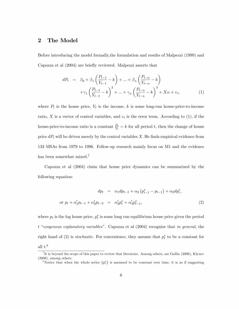
Before introducing the model formally,the formulation and results of Malpezzi (1999) and
Capozza et al (2004) are briefly reviewed. Malpezzi asserts that
= 0 + 1
µ−1−1
−
¶+ +
µ−−
−
¶+1
µ−1−1
−
¶3+ +
µ−−
−
¶3++ (1)
where is the house price, is the income, is some long-run house-price-to-income
ratio, is a vector of control variables, and is the error term. According to (1), if the
house-price-to-income ratio is a constant = for all period , then the change of house
price will be driven merely by the control variables He finds empirical evidence from
133 MSAs from 1979 to 1996. Follow-up research mainly focus on M1 and the evidence
has been somewhat mixed.7
Capozza et al (2004) claim that house price dynamics can be summarized by the
following equation:
= 1−1 + 2¡∗−1 − −1
¢+ 3
∗
or + 01−1 + 02−2 = 03∗ + 04
∗−1 (2)
where is the log house price, ∗ is some long run equilibrium house price given the period
“exogenous explanatory variables”. Capozza et al (2004) recognize that in general, the
right hand of (2) is stochastic. For convenience, they assume that ∗ to be a constant for
all .8
7 It is beyond the scope of this paper to review that literature. Among others, see Gallin (2006), Klyuev
(2008), among others.8Notice that when the whole series {∗ } is assumed to be constant over time, it is as if suggesting
6
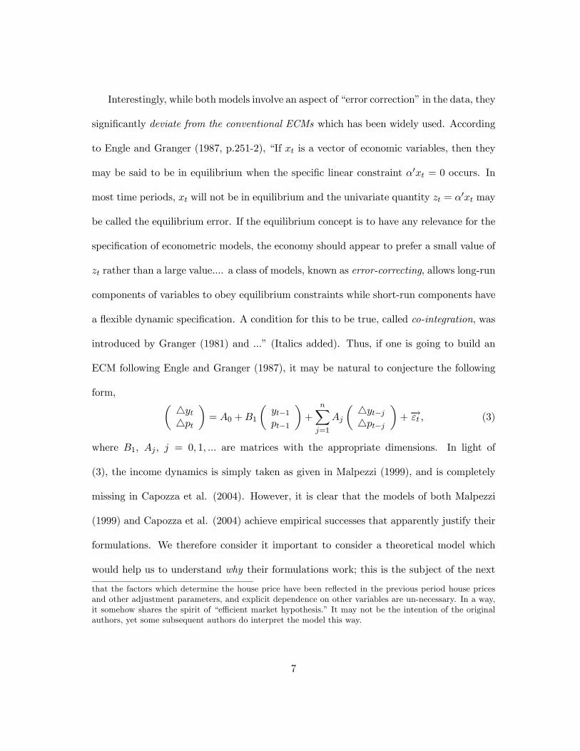
Interestingly, while both models involve an aspect of “error correction” in the data, they
significantly deviate from the conventional ECMs which has been widely used. According
to Engle and Granger (1987, p.251-2), “If is a vector of economic variables, then they
may be said to be in equilibrium when the specific linear constraint 0 = 0 occurs. In
most time periods, will not be in equilibrium and the univariate quantity = 0 may
be called the equilibrium error. If the equilibrium concept is to have any relevance for the
specification of econometric models, the economy should appear to prefer a small value of
rather than a large value.... a class of models, known as error-correcting, allows long-run
components of variables to obey equilibrium constraints while short-run components have
a flexible dynamic specification. A condition for this to be true, called co-integration, was
introduced by Granger (1981) and ...” (Italics added). Thus, if one is going to build an
ECM following Engle and Granger (1987), it may be natural to conjecture the following
form, µ 44
¶= 0 +1
µ−1−1
¶+
X=1
µ 4−4−
¶+−→ (3)
where 1, , = 0 1 are matrices with the appropriate dimensions. In light of
(3), the income dynamics is simply taken as given in Malpezzi (1999), and is completely
missing in Capozza et al. (2004). However, it is clear that the models of both Malpezzi
(1999) and Capozza et al. (2004) achieve empirical successes that apparently justify their
formulations. We therefore consider it important to consider a theoretical model which
would help us to understand why their formulations work; this is the subject of the next
that the factors which determine the house price have been reflected in the previous period house prices
and other adjustment parameters, and explicit dependence on other variables are un-necessary. In a way,
it somehow shares the spirit of “efficient market hypothesis.” It may not be the intention of the original
authors, yet some subsequent authors do interpret the model this way.
7
section.
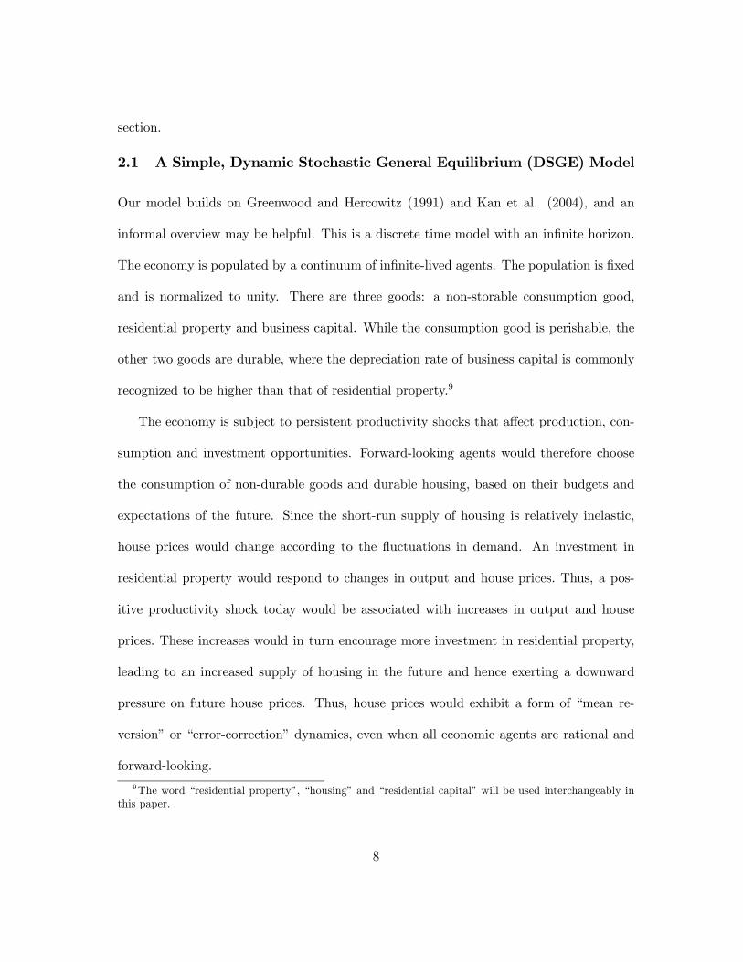
2.1 A Simple, Dynamic Stochastic General Equilibrium (DSGE) Model
Our model builds on Greenwood and Hercowitz (1991) and Kan et al. (2004), and an
informal overview may be helpful. This is a discrete time model with an infinite horizon.
The economy is populated by a continuum of infinite-lived agents. The population is fixed
and is normalized to unity. There are three goods: a non-storable consumption good,
residential property and business capital. While the consumption good is perishable, the
other two goods are durable, where the depreciation rate of business capital is commonly
recognized to be higher than that of residential property.9
The economy is subject to persistent productivity shocks that affect production, con-
sumption and investment opportunities. Forward-looking agents would therefore choose
the consumption of non-durable goods and durable housing, based on their budgets and
expectations of the future. Since the short-run supply of housing is relatively inelastic,
house prices would change according to the fluctuations in demand. An investment in
residential property would respond to changes in output and house prices. Thus, a pos-
itive productivity shock today would be associated with increases in output and house
prices. These increases would in turn encourage more investment in residential property,
leading to an increased supply of housing in the future and hence exerting a downward
pressure on future house prices. Thus, house prices would exhibit a form of “mean re-
version” or “error-correction” dynamics, even when all economic agents are rational and
forward-looking.
9The word “residential property”, “housing” and “residential capital” will be used interchangeably in
this paper.
8

More formally, in each period , = 1 2,..., the representative agent maximizes the
expected value of the lifetime utility
∞X=
− ( ) which is the discounted
sum of the periodic utility ( ) where is the discounted factor, 0 1
is the amount of consumption in period , is the stock of housing (or, residential
property; these terms are used interchangeably throughout this paper) owned by the
representative agent in period , and is the number of working hours provided by the
agent, 0 , = (+ 1), .... Following the literature, we assume that the preference
of the representative agent is separable. Formally, the utility function takes the following
form,
() = ln + ln − ()
1+
1 + (4)
where both and are positive preference parameters determining consumers’ resource
allocation among consumption, residential property and leisure. The assumed positivity
of ensures that the labor supply curve is upward sloping.
The production side is relatively simple. The goods production technology is repre-
sented by a Cobb-Douglas function,
= () ()
1− (5)
where 0 1 and exhibits constant return to scale in business capital and labor.
Throughout this paper, the terms “output” and “income” will be used interchangeably for
. The amount of output, however, depends not only on the amount of business capital
and labor, but also on productivity , which fluctuates over time. In the macroeconomic
literature, it is commonly assumed that the log of productivity follows an AR(1) process,
= −1 + (6)
9
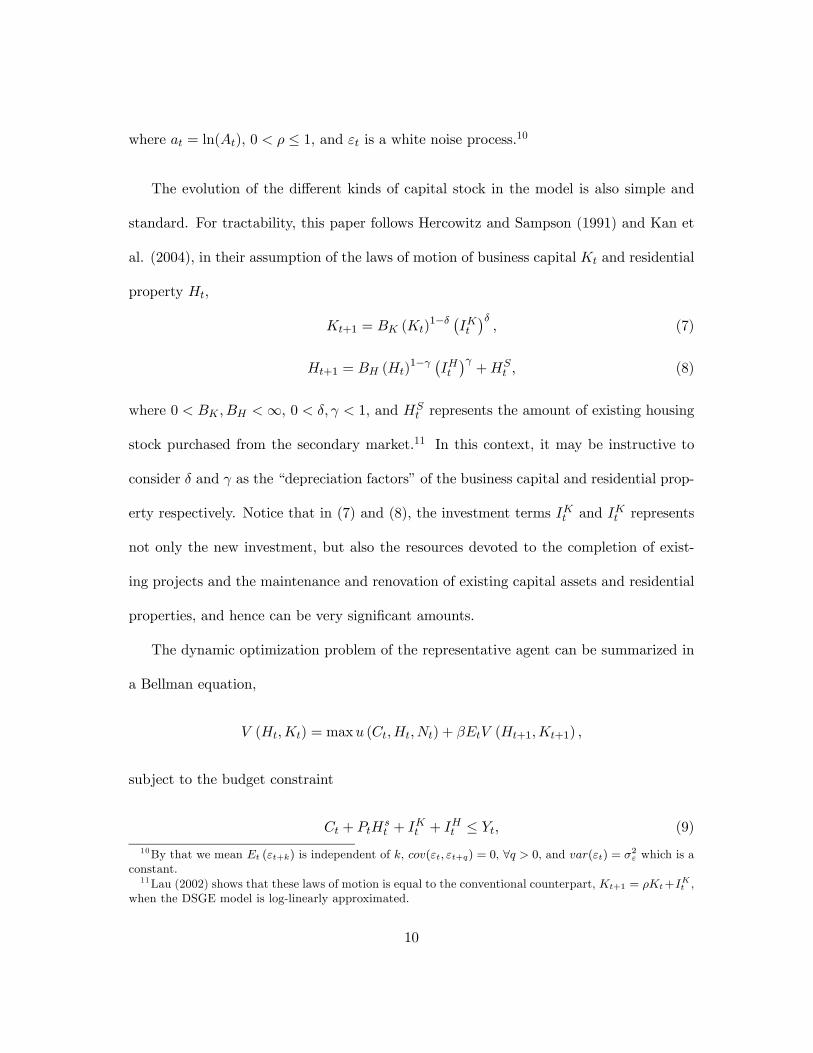
where = ln(), 0 ≤ 1, and is a white noise process.10
The evolution of the different kinds of capital stock in the model is also simple and
standard. For tractability, this paper follows Hercowitz and Sampson (1991) and Kan et
al. (2004), in their assumption of the laws of motion of business capital and residential
property ,
+1 = ()1− ¡ ¢ (7)
+1 = ()1− ¡ ¢ +
(8)
where 0 ∞, 0 1 and represents the amount of existing housing
stock purchased from the secondary market.11 In this context, it may be instructive to
consider and as the “depreciation factors” of the business capital and residential prop-
erty respectively. Notice that in (7) and (8), the investment terms and represents
not only the new investment, but also the resources devoted to the completion of exist-
ing projects and the maintenance and renovation of existing capital assets and residential
properties, and hence can be very significant amounts.
The dynamic optimization problem of the representative agent can be summarized in
a Bellman equation,
() = max ( ) + (+1+1)
subject to the budget constraint
+ + + ≤ (9)
10By that we mean (+) is independent of , ( +) = 0, ∀ 0, and () = 2 which is a
constant.11Lau (2002) shows that these laws of motion is equal to the conventional counterpart, +1 = +
,
when the DSGE model is log-linearly approximated.
10
and the laws of motion for capital and housing, (7) and (8), where ( ) is given
by (4) and is given by (5). Implicitly, it is assumed that the representative agent can
buy or sell existing housing stock at unit price .
To solve this rather complicated system of equations, equilibrium conditions need to
be imposed. Following Lucas (1978), we impose the natural restriction that the net sale
of residential properties among agents is zero in equilibrium,
= 0, ∀ (10)
Equipped with all these conditions, we are now ready to define the stationary equilib-
rium of the model.
Definition 1 For a given sequence of productivity shocks {}∞=0, a stationary equilib-
rium is a sequence of quantities©
ª∞=0
, and a sequence of housing
prices {}∞=0, such that the representative agent maximizes his expected life-time utility,
subject to the constraints (7), (8), and (9), Meanwhile, the housing market clears, implying
equation (10) holds.
In this model, the equilibrium can be solved explicitly. The solution strategy is simple.
The quantities are solved first, and are then followed by prices. All proofs are presented
in the appendix. We first show that the equilibrium quantities can be characterized by
the following equations.
Proposition 1 Under some conditions, the evolution of the equilibrium quantities can be
11
characterized by these following equations:
=
=
=
= (11)
for some constant , , and , such that 0 , , 1, 0
A few comments may improve understanding of the intuitions behind the results.
Intuitively, if there is a good productivity shock, then output is expected to increase.
The income effect encourages the economic agents to increase the consumption-to-output
ratio. On the other hand, the substitution effect suggests the economic agent to invest more
because with more output, the marginal cost of investment decreases. Since our utility
function is in log form, the income effect and substitution effect exactly offset each other.
And with some technical conditions that are detailed in the appendix, the consumption-
to-output ratio and different investment-to-output ratios in the model remain constant. In
addition, the utility from is separable, and hence the labor supply depends on the product
of the marginal utility of consumption and the output, (1 ) Intuitively, if there is a
good productivity shock, then output is expected to increase. However, with a higher
income, consumption will also increase, so that marginal utility of consumption 1 will
decrease. And with our separable log utility functional form, the two effects exactly offset
each other and hence the labor supply becomes constant.
Using (11), we can further characterize the entire dynamical system. First, we take
the natural logarithm for different variables. For instance, = ln = ln etc. This
12
procedure not only facilitates the subsequent analysis, but is also the procedures used in
many empirical works and hence facilitates communication between the theoretical and
empirical work in this area. Notice further that most control variables depend on the
output , which in turns depends on the productivity shock, capital stock and labor (see
equation (5)). Following Sargent (1979), it is in fact a block-recursive system, meaning
that once we solve the dynamics of the “core” sub-system, the entire dynamical system can
be easily solved. Formally, it means that the model economy is described by the following
equation system,
= + +
+1 = + (1− ) +
+1 = + (1− ) +
= +
= + (12)
where , , , , , are all constant. Note further that (12) is driven by a “core”
sub-system, which is the vector −→ where
−→ =
µ
The following result describes the dynamics of −→
Proposition 2 The dynamics of −→ is dictated by the following vector equation,
−→ +1 =0 +1−→ +
−→ +1 (13)
where 0, 1are matrices of constant,−→ is a vector of shock terms,
−→ =
µ+10
¶ In
fact, we can express, in log form, the output, physical capital stock, and residential housing
13
stock as a summation of previous period productivity shocks,
= 00 + + ()
∞X=0
(1− + ) −1−
= 00 +
∞X=0
(1− + ) −1−
= 00 + −1 +
∞X=0
() −2− (14)
where 00, = , , are constant, () is a function of parameters and .
In a sense, this result is not very surprising. For instance, Slutzky (1937) shows that
a cyclical stochastic process can be decomposed as a summation of uncorrelated random
variables. Thus, (14) can be interpreted as a re-statement of Slutsky’s result in a DSGE
context. A consequence of (14) is that the stochastic properties of the economic variables
(the output , physical capital stock , and residential housing stock ) will depend on
the stochastic properties of the productivity shock Following Cooley (1995), we assume
that the productivity shock follows an AR(1) process, as reflected by (6). Empirically, the
productivity shock process is not only serially correlated, but is also very close to unit root
(Cooley, 1995). According to some authors, the persistence parameter, is sometimes
statistically indistinguishable from unity. We will therefore study both the case of “mean-
reverting” (or “temporary”) case, i.e. where 0 1 and the case of “unit root” (or
“permanent”) case, i.e. where = 1. For simplification, we will focus on the case of
mean-reverting productivity shock in the text and present the case of permanent shock in
the appendix.
Proposition 3 The stationarity of depends on the persistency of the productivity shock
which is defined in (6). In particular, when we express in the form ofP∞
=0 () −,
14
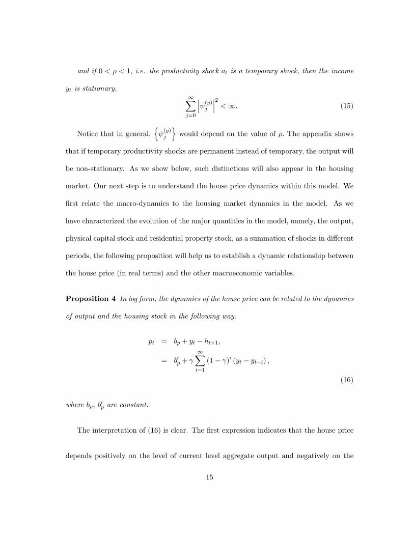
and if 0 1 i.e. the productivity shock is a temporary shock, then the income
is stationary,∞X=0
¯̄̄()
¯̄̄2∞ (15)
Notice that in general,n()
owould depend on the value of The appendix shows
that if temporary productivity shocks are permanent instead of temporary, the output will
be non-stationary. As we show below, such distinctions will also appear in the housing
market. Our next step is to understand the house price dynamics within this model. We
first relate the macro-dynamics to the housing market dynamics in the model. As we
have characterized the evolution of the major quantities in the model, namely, the output,
physical capital stock and residential property stock, as a summation of shocks in different
periods, the following proposition will help us to establish a dynamic relationship between
the house price (in real terms) and the other macroeconomic variables.
Proposition 4 In log form, the dynamics of the house price can be related to the dynamics
of output and the housing stock in the following way:
= + − +1
= 0 +
∞X=1
(1− ) ( − −)
(16)
where , 0 are constant.
The interpretation of (16) is clear. The first expression indicates that the house price
depends positively on the level of current level aggregate output and negatively on the
15
foreseen amount of residential property stock. Thus, other things being equal, an antic-
ipation of an increase in the future stock of housing will depress the house price today.
The house price is “forward-looking” in this sense. The second expression requires more
explanation. Notice that, by definition, the term ( − −) = ln−ln− = ln(−)
which is the economic growth between period and ( − ). Thus, the second expression
indicates that the house price (in real terms) can be interpreted as a weighted sum of
the economic growth between the current period and different previous periods. Higher
economic growth leads to a higher house price. Notice that the weight allocated to the
economic growth between period and ( − ) is (1− ). As 0 (1− ) 1 the value
of the term (1− ) decreases with , such that periods of more distant past (i.e. higher
values of ) will carry less weight. In other words, if the output level at some particular
time 0 is unusually high, it would lead to a higher level of house price 0 . The impact,
however, will die off over time. It is because if 0 is unusually high, then for 0,
it is likely that ( − 0) will become small and hence will constrain further increase in
house price. The model thus implies that continuous increase in house price can only be
sustained by persistent economic growth.
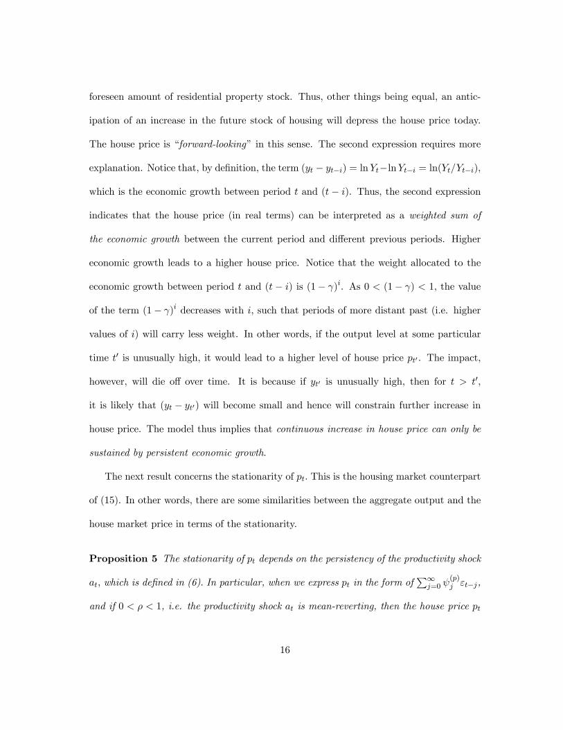
The next result concerns the stationarity of This is the housing market counterpart
of (15). In other words, there are some similarities between the aggregate output and the
house market price in terms of the stationarity.
Proposition 5 The stationarity of depends on the persistency of the productivity shock
which is defined in (6) In particular, when we express in the form ofP∞
=0 () −,
and if 0 1, i.e. the productivity shock is mean-reverting, then the house price
16
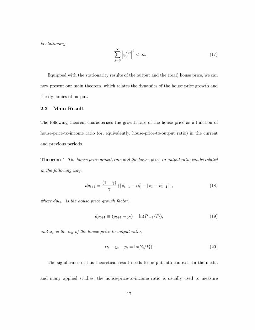
is stationary,∞X=0
¯̄̄()
¯̄̄2∞ (17)
Equipped with the stationarity results of the output and the (real) house price, we can
now present our main theorem, which relates the dynamics of the house price growth and
the dynamics of output.
2.2 Main Result
The following theorem characterizes the growth rate of the house price as a function of
house-price-to-income ratio (or, equivalently, house-price-to-output ratio) in the current
and previous periods.
Theorem 1 The house price growth rate and the house price-to-output ratio can be related
in the following way:
+1 =(1− )
{[κ+1 − κ]− [κ − κ−1]} (18)
where +1 is the house price growth factor,
+1 ≡ (+1 − ) = ln(+1) (19)
and κ is the log of the house price-to-output ratio,
κ ≡ − = ln() (20)
The significance of this theoretical result needs to be put into context. In the media
and many applied studies, the house-price-to-income ratio is usually used to measure
17
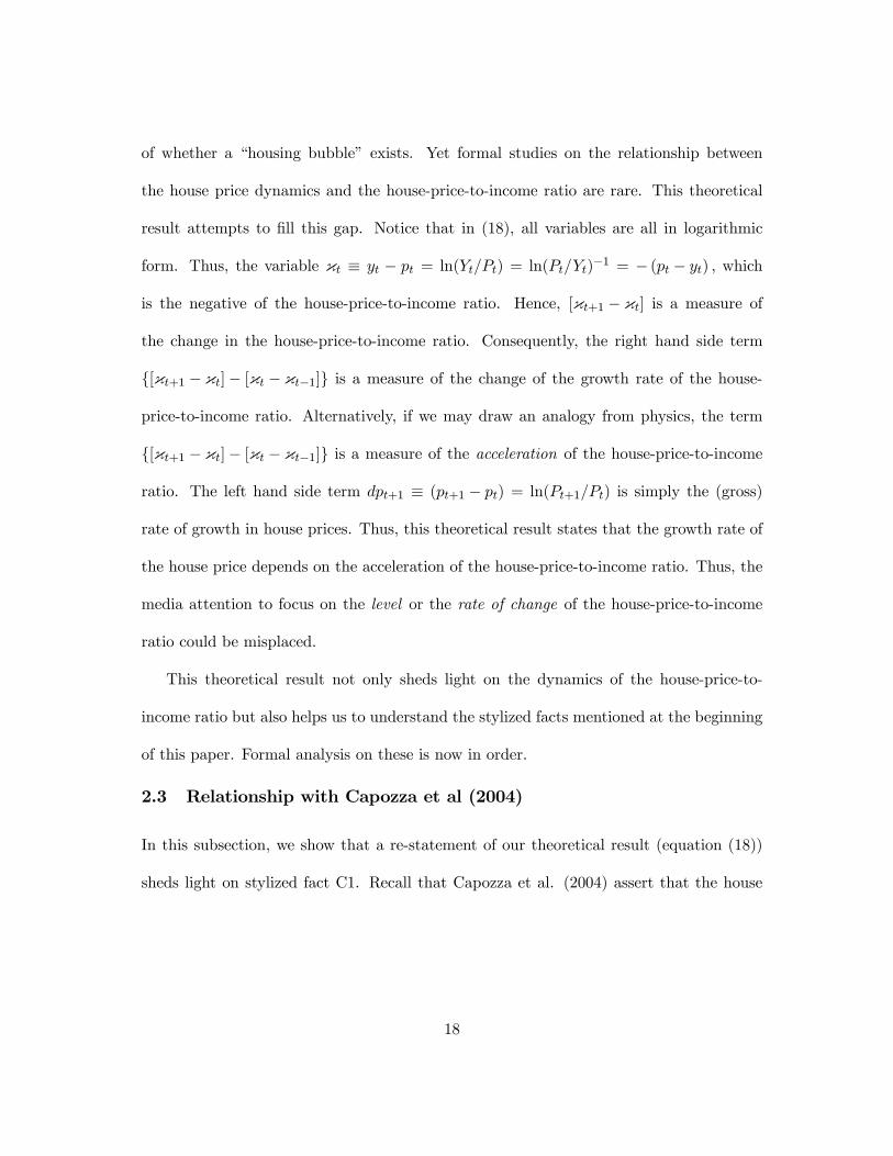
of whether a “housing bubble” exists. Yet formal studies on the relationship between
the house price dynamics and the house-price-to-income ratio are rare. This theoretical
result attempts to fill this gap. Notice that in (18), all variables are all in logarithmic
form. Thus, the variable κ ≡ − = ln() = ln()−1 = − ( − ) which
is the negative of the house-price-to-income ratio. Hence, [κ+1 − κ] is a measure of
the change in the house-price-to-income ratio. Consequently, the right hand side term
{[κ+1 − κ]− [κ − κ−1]} is a measure of the change of the growth rate of the house-
price-to-income ratio. Alternatively, if we may draw an analogy from physics, the term
{[κ+1 − κ]− [κ − κ−1]} is a measure of the acceleration of the house-price-to-income
ratio. The left hand side term +1 ≡ (+1 − ) = ln(+1) is simply the (gross)
rate of growth in house prices. Thus, this theoretical result states that the growth rate of
the house price depends on the acceleration of the house-price-to-income ratio. Thus, the
media attention to focus on the level or the rate of change of the house-price-to-income
ratio could be misplaced.
This theoretical result not only sheds light on the dynamics of the house-price-to-
income ratio but also helps us to understand the stylized facts mentioned at the beginning
of this paper. Formal analysis on these is now in order.
2.3 Relationship with Capozza et al (2004)
In this subsection, we show that a re-statement of our theoretical result (equation (18))
sheds light on stylized fact C1. Recall that Capozza et al. (2004) assert that the house
18
prices follow a second-order equation, (2),
= 1−1 + 2¡∗−1 − −1
¢+ 3
∗
or + 01−1 + 02−2 = 03∗ + 04
∗−1
where , = 1 2 3 are parameters to be estimated, is defined in (19), and ∗ is some
long-run equilibrium house price given the period “exogenous explanatory variables”.
Capozza et al. (2004) recognize that, in general, the right-hand side is stochastic. For
convenience, they assume that ∗ to be a constant for all . Interestingly, they find
empirical support for their formulation. The next proposition shows that we can also
re-write (18) in a comparable manner.
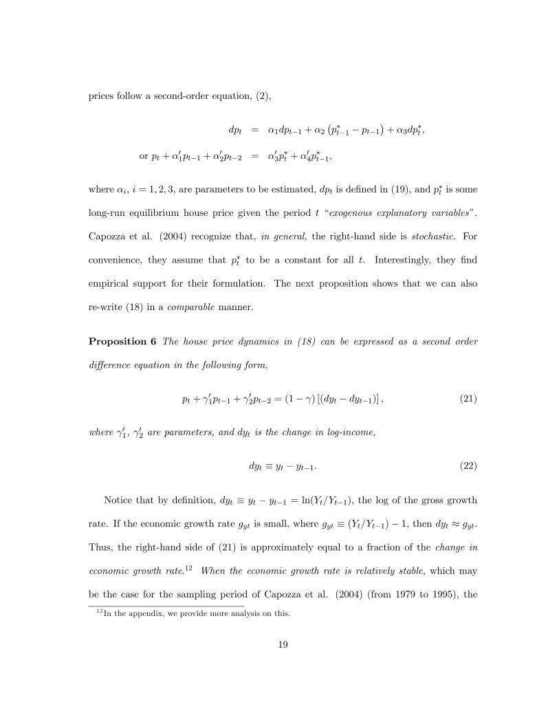
Proposition 6 The house price dynamics in (18) can be expressed as a second order
difference equation in the following form,
+ 01−1 + 02−2 = (1− ) [( − −1)] (21)
where 01, 02 are parameters, and is the change in log-income,
≡ − −1 (22)
Notice that by definition, ≡ − −1 = ln(−1) the log of the gross growth
rate. If the economic growth rate is small, where ≡ (−1)− 1, then ≈
Thus, the right-hand side of (21) is approximately equal to a fraction of the change in
economic growth rate.12 When the economic growth rate is relatively stable, which may
be the case for the sampling period of Capozza et al. (2004) (from 1979 to 1995), the
12 In the appendix, we provide more analysis on this.
19
right-hand side of (21) can indeed be approximated by a constant. In other words, the
assumption made in Capozza et al. (2004) may be justifiable not only on the empirical
ground, but also on theoretical grounds when the economic growth rate does not vary too
much. Therefore, the dynamic model proposed here provides an equilibrium interpretation
of the empirical results in Capozza et al. (2004).
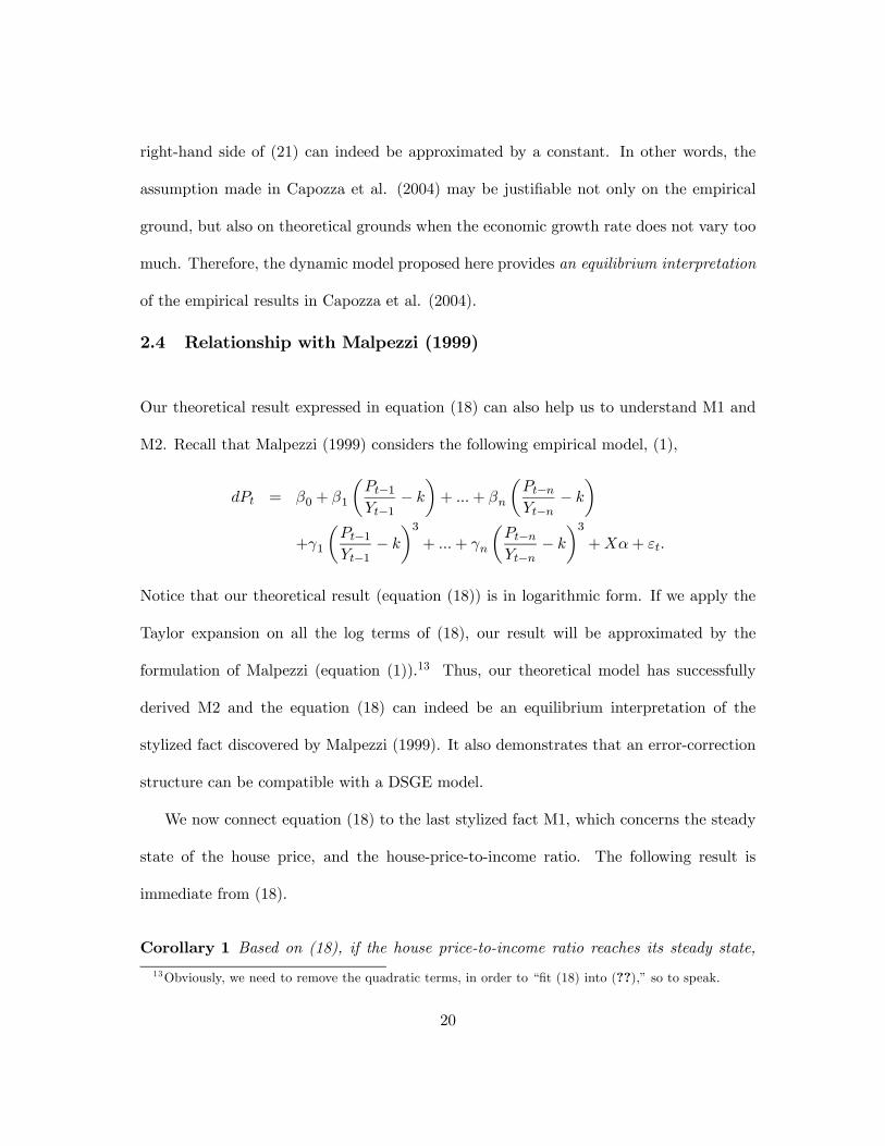
2.4 Relationship with Malpezzi (1999)
Our theoretical result expressed in equation (18) can also help us to understand M1 and
M2. Recall that Malpezzi (1999) considers the following empirical model, (1),
= 0 + 1
µ−1−1
−
¶+ +
µ−−
−
¶+1
µ−1−1
−
¶3+ +
µ−−
−
¶3++
Notice that our theoretical result (equation (18)) is in logarithmic form. If we apply the
Taylor expansion on all the log terms of (18), our result will be approximated by the
formulation of Malpezzi (equation (1)).13 Thus, our theoretical model has successfully
derived M2 and the equation (18) can indeed be an equilibrium interpretation of the
stylized fact discovered by Malpezzi (1999). It also demonstrates that an error-correction
structure can be compatible with a DSGE model.
We now connect equation (18) to the last stylized fact M1, which concerns the steady
state of the house price, and the house-price-to-income ratio. The following result is
immediate from (18).
Corollary 1 Based on (18), if the house price-to-income ratio reaches its steady state,
13Obviously, we need to remove the quadratic terms, in order to “fit (18) into (??),” so to speak.
20
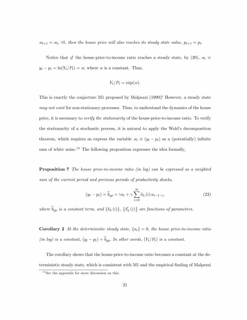
κ+1 = κ, ∀, then the house price will also reaches its steady state value, +1 = .
Notice that if the house-price-to-income ratio reaches a steady state, by (20), κ ≡
− = ln() = κ where κ is a constant. Thus,
= exp(κ)
This is exactly the conjecture M1 proposed by Malpezzi (1999)! However, a steady state
may not exist for non-stationary processes. Thus, to understand the dynamics of the house
price, it is necessary to verify the stationarity of the house-price-to-income ratio. To verify
the stationarity of a stochastic process, it is natural to apply the Wold’s decomposition
theorem, which requires us express the variable κ ≡ ( − ) as a (potentially) infinite
sum of white noise.14 The following proposition expresses the idea formally,
Proposition 7 The house price-to-income ratio (in log) can be expressed as a weighted
sum of the current period and previous periods of productivity shocks,
( − ) = b + +
∞X=0
() −1− (23)
where b is a constant term, and { ()}, ©0 ()ª are functions of parameters.Corollary 2 At the deterministic steady state, {} = 0, the house price-to-income ratio
(in log) is a constant, ( − ) = b In other words, () is a constant.The corollary shows that the house-price-to-income ratio becomes a constant at the de-
terministic steady state, which is consistent with M1 and the empirical finding of Malpezzi
14See the appendix for more discussion on this.
21

(1999). In general, however, {} 6= 0. Moreover, as we have assumed in (6), it is seri-
ally correlated, i.e. ( −) 6= 0 for 0. Thus, to verify the stationarity of the
house-price-to-income ratio ( − ) we need to express it as an infinite sum of seri-
ally uncorrelated disturbance terms, following the Wold’s decomposition theorem. The
following proposition addresses this.
Proposition 8 Assume that (6) holds. We can then write the house price-to-income ratio
in the following form,
( − ) = b + ∞X=0
0 () − (24)
where is a white noise. Furthermore, if 0 1, i.e. the productivity shock is a
temporary shock, the stochastic process of log house price-to-income ratio is stationary
∞X=0
¯̄0 ()
¯̄2∞ (25)
The intuition of the result is simple. If the productivity shock is temporary (0 1),
a positive shock today may not have much impact on the discounted lifetime wealth as
the representative agent rationally expects a future negative shock to offset the current
period’s positive shock. As a result, the house price does not increase much and the house
price-to-income ratio remains stationary. In the empirical literature, many authors do not
consider whether the house-price-to-income ratio is stationary. Instead, they investigate
whether house prices and income are co-integrated. Interestingly, our model can also shed
light on this issue. Notice that in logarithmic form, the house-price-to-income ratio is
22
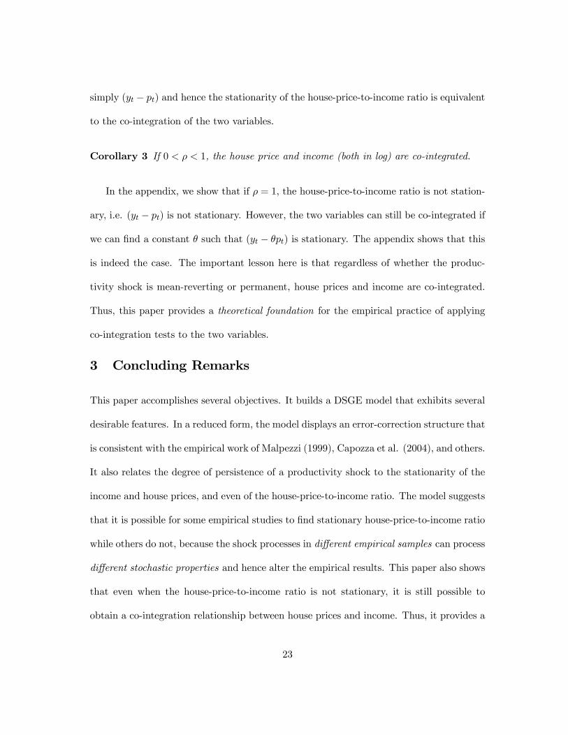
simply ( − ) and hence the stationarity of the house-price-to-income ratio is equivalent
to the co-integration of the two variables.
Corollary 3 If 0 1, the house price and income (both in log) are co-integrated.
In the appendix, we show that if = 1, the house-price-to-income ratio is not station-
ary, i.e. ( − ) is not stationary. However, the two variables can still be co-integrated if
we can find a constant such that ( − ) is stationary. The appendix shows that this
is indeed the case. The important lesson here is that regardless of whether the produc-
tivity shock is mean-reverting or permanent, house prices and income are co-integrated.
Thus, this paper provides a theoretical foundation for the empirical practice of applying
co-integration tests to the two variables.
3 Concluding Remarks
This paper accomplishes several objectives. It builds a DSGE model that exhibits several
desirable features. In a reduced form, the model displays an error-correction structure that
is consistent with the empirical work of Malpezzi (1999), Capozza et al. (2004), and others.
It also relates the degree of persistence of a productivity shock to the stationarity of the
income and house prices, and even of the house-price-to-income ratio. The model suggests
that it is possible for some empirical studies to find stationary house-price-to-income ratio
while others do not, because the shock processes in different empirical samples can process
different stochastic properties and hence alter the empirical results. This paper also shows
that even when the house-price-to-income ratio is not stationary, it is still possible to
obtain a co-integration relationship between house prices and income. Thus, it provides a
23
micro-foundation for the empirical practices in the literature of applying the co-integration
test between house prices and income. In addition, as this paper demonstrates that it is
possible for a DSGE model to have an error-correction structure, the empirical validity
of the error-correction model can be consistent with an equilibrium interpretation of the
dynamics of output and house prices.
This paper makes several simplifying assumptions, which naturally become limitations.
We will briefly discuss these here and leave it to future studies to improve on these di-
mensions. First, this paper assumes that there is only a national housing market and only
one source of shock that affects both the aggregate output and the housing market. In
practice, different regional housing markets may be subject to different shocks and may
behave differently.15 To address the regional heterogeneity, this model needs to be ex-
tended to allow for the existence of (ex post) heterogeneous regions and to possibly allow
for region-specific shocks to affect different regions. In addition, regional labor markets
and, in general, the “frictions” involved in any factor (labor, capital, . . . ) to move across
regions, or even the financial instruments available for agents to diversify risk, may affect
the regional house price dynamics.16 Clearly, more research is needed into the equilibrium
prediction of regional house price dynamics.
As the current paper focuses on the productivity shock as a driving force for both the
aggregate output and house prices, it inevitably ignores other channels. For instance, the
15Among others, see Davidoff (2013) for a review of the literature.16Recently, there are some attemtps along this line. For instance, Leung and Teo (2011) study a multi-
region DSGE with both aggregate and region-specific shocks. They allow agents to hold stock as well
as housing in their portfolio. However, they did not allow for agents to move across regions. They find
that, numerically, the short run dynamics of regional house price can be very different, depending on the
region-specific adjustment cost of housing stock. On the other hand, Van Nieuwerburgh and Weill (2012)
allow agents to be freely mobile. However, they assume agents to have linear preference non-durable
consumption goods, and thus eliminating the need to insure for non-durable consumption risk. They focus
on the house price dispersion and do not examine the house price dynamics.
24
model could be enriched by introducing household production.17 Among others, Davis
and Martin (2009) and Dong et al. (2013) show, numerically, that introducing house-
hold production can improve the data-matching performance of a conventional business
cycle model with housing. However, they do not explore the evolution of the house price
dynamics analytically, and do not relate the house price dynamics to the dynamics of
house-price-to-income ratio. Recently, Mian and Sufi (2010) and Mian et al. (2010),
among others, provide micro-evidence that the mortgage supply and the political econ-
omy may be important in explaining why some counties have been affected more severely
than others by the Great Recession. There are tractable models on how mortgage sup-
ply and house prices are both endogenously determined in a dynamic equilibrium setting,
such as Chen et al. (2012), Chen and Leung (2008) and Jin et al. (2012). Chen et al.
(2012) and Jin et al. (2012) both numerically matches some aspects of the housing market
reasonably well. However, adding the political economy in any of these models may be
very involved.18 We can thus only recognize these as limitations and leave them for future
research.
17Greenwood et al (1995) show that the reduced form of models with household production that is
subject to stochastic productivity shock may not be distinguishable from models with taste shock.18Clearly, it is beyond the scope of this paper to explain the potential difficulties to extend an economic
model to a political economy model. Among others, see Acemoglu and Robinson (2009), Banks and
Hanushek (1995), Persson and Tabellini, 2002.
25

References
[1] Acemoglu, D. and J. Robinson, 2009, Economic Origins of Dictatorship and Democ-
racy, Cambridge: Cambridge University Press.
[2] Banks, J. and E. Hanushek ed., 1995, Modern Political Economy: Old Topics, New
Directions, Cambridge: Cambridge University Press.
[3] Bartle, R. and D. Sherbert, 2011, Introduction to Real Analysis, 4th ed., New York:
Wiley.
[4] Capozza, D.; P. H. Hendershott, and C. Mack, 2004, An Anatomy of Price Dynamics
in Illiquid Markets: Analysis and Evidence from Local Housing Markets, Real Estate
Economics, 32, 1-32.
[5] Chang, K. L.; N. K. Chen and C. K. Y. Leung, 2011, Monetary Policy, Term Structure
and Real Estate Return: Comparing REIT, housing and stock, Journal of Real Estate
Finance and Economics, 43, 221-257.
[6] Chen, N. K.; Cheng, H. L. and C. S. Mao, 2012, House price, mortgage premium,
and business fluctuations, Economic Modelling, 29(4), 1388-1398.
[7] Chen, N. K. and C. K. Y. Leung, 2008, Asset Price Spillover, Collateral and Crises:
with an Application to Property Market Policy, Journal of Real Estate Finance and
Economics, 37, 351-385.
[8] Cooley, T., ed., 1995, Frontiers of Business Cycle Research, Princeton: Princeton
University Press.
[9] Davidoff, T. 2013, Supply Elasticity and the Housing Cycle of the 2000s, forthcoming
in Real Estate Economics.
[10] Davis, M. and J. Heathcote, 2005, Housing and the business cycle, International
Economic Review, 46, 751-784.
[11] Davis, M. and F. Martin, 2009, Housing, home production, and the equity- and
value-premium puzzles, Journal of Housing Economics, 18, 81-91.
[12] Dong, J., F. Y. Kwan and C. K. Y. Leung, 2013, Comparing consumption-based asset
pricing models, working paper.
[13] Economist, 2011, Central Banks: a more complicated game, 17th Feburary,
http://www.economist.com/node/18178251.
[14] Elaydi, S., 2005, An Introduction to Difference Equations, 3rd ed., New York:
Springer.
26
[15] Engle, R. and C. Granger, 1987, Co-integration and error correction: representation,
estimation and testing, Econometrica 55, 251—76.
[16] Farmer, R. E.A.; D. Waggoner and T. Zha, 2009, Understanding Markov-switching
rational expectations models, Journal of Economic Theory, 144(5), 849-1867.
[17] Fernandez-Villaverde, J., 2010, The econometrics of DSGE models, SERIEs, 1, 3-49.
[18] Gallin, J., 2006, The long-run relationship between house prices and income: evidence
from local housing markets, Real Estate Economics, 34, 417-438.
[19] Glindro, E.; T. Subhanij, J. Szeto, and H. Zhu, 2011, Determinants of House Prices
in Nine Asia-Pacific Economies, International Journal of Central Banking, 7, 163-204.
[20] Granger, C., 1981, Some Properties of Time Series Data and Their Use in Econometric
Model Specification, Journal of Econometrics, 121-130.
[21] Greenwood, J. and Z. Hercowitz, 1991, The allocation of capital and time over the
business cycle, Journal of Political Economy, 99, 1188-1214.
[22] Greenwood, J.; R. Rogerson, and R. Wright, 1995, Household Production in Real
Business Cycle Theory, in Frontiers of Business Cycle Research, ed. by T. F. Cooley,
Princeton: Princeton University Press, 157-174.
[23] Hamilton, J., 1994, Time Series Analysis, Princeton: Princeton University Press.
[24] Hardy, G. H., J. E. Littlewood and G. Polya, 1934, Inequalities, Cambridge: Cam-
bridge University Press.
[25] Hercowitz, Z. and M. Sampson, 1991, Output, growth, the real wage, and employment
fluctuations, American Economic Review, 81, 1215-37.
[26] Iacoviello, M., 2005, House Prices, Borrowing Constraints, and Monetary Policy in
the Business Cycle, American Economic Review, 95, 739-764.
[27] Iacoviello, M., and S. Neri, 2010, Housing Market Spillovers: Evidence from an Esti-
mated DSGE Model, American Economic Journal: Macroeconomics, 2, 125-164.
[28] Iacoviello, M., and M. Pavan, 2012, Housing and Debt Over the Life Cycle and Over
the Business Cycle, forthcoming in Journal of Monetary Economics.
[29] Jin, Y.; C. K. Y. Leung and Z. Zeng, 2012, Real Estate, the External Finance Pre-
mium and Business Investment: A Quantitative Dynamic General Equilibrium Analy-
sis, Real Estate Economics, 40(1), 167-195.
[30] Jin, Y. and Z. Zeng, 2007, Real estate and optimal public policy in a credit-constrained
economy, Journal of Housing Economics, 16(2), 143-166.
27
[31] Kan, K.; Kwong, S. K. S.;C. K. Y. Leung, 2004, The dynamics and volatility of
commercial and residential property prices: theory and evidence, Journal of Regional
Science, 44(1), 95-123.
[32] Keep, M., 2012, Regional house prices: affordability and income ratios, Standard
Note SN/SG/1922, Library, House of Commons, Parliament of the United Kingdom.
[33] King, R.; C. Plosser and S. Rebelo, 2002, Production, Growth and Business Cycles:
Technical Appendix, Computational Economics, 20, 87-116.
[34] King, R.; C. Plosser, J. Stock and M. Watson, 1991, Stochastic trends and economic
fluctuations, American Economic Review, 81(4), 819-840.
[35] Klyuev, V., 2008, What goes up must come down? house price dynamics in the
United States, IMF Working Paper.
[36] Kydland, F. E. and E. C. Prescott, 1996, The Computational Experiment: An Econo-
metric Tool, Journal of Economic Perspectives, 10(1), 69-85.
[37] Lau, S. H., 2002, Further inspection of the stochastic growth model by an analytical
approach, Macroeconomic Dynamics, 6(5), 748-757.
[38] Leung, C., 2004, Macroeconomics and Housing: a review of the literature, Journal of
Housing Economics, 13, 249-267.
[39] Leung, C. K. Y. and W. L. Teo, 2011, Should the optimal portfolio be region-specific?
A multi-region model with monetary policy and asset price co-movements, Regional
Science and Urban Economics, 41, 293-304.
[40] Lucas, R., 1978, Asset Prices in an exchange economy, Econometrica, 46, 1426-45.
[41] Malpezzi, S., 1999, A Simple Error Correction Model of House Prices, Journal of
Housing Economics, 8, 27-62.
[42] Mian, A. and A. Sufi, 2010, The Great Recession: lessons form microeconomic data,
American Economic Review: Papers and Proceedings, 100, 51-56.
[43] Mian, A.; A. Sufi and F. Trebbi, 2010, The political economy of the US mortgage
default crisis, American Economic Review, 100, 1967-1998.
[44] Ortalo-Magne, F. and S. Rady, 2006, Housing Market Dynamics: On the Contribution
of Income Shocks and Credit Constraints, Review of Economic Studies, 73, 459—485.
[45] Persson, T. and G. Tabellini, 2002, Political Economics: Explaining Economic Policy
(Zeuthen Lectures), Cambridge: MIT Press.
28

[46] Ried, S. and H. Uhlig, 2009, The macroeconomics of real estate, Humboldt-Universitat
zu Berlin, working paper.
[47] Sargent, T., 1979, Macroeconomic Theory, New York: Academic Press.
[48] Sargent, T., 1987, Dynamic Macroeconomic Theory, Cambridge: Harvard University
Press.
[49] Slutzky, E., 1937, The Summation of Random Causes as the Source of Cyclic
Processes, Econometrica, 5(2), 105-146.
[50] Sowell, T., 2009, The Housing Boom and Bust, rev. ed., New York: Basic Books.
[51] Steele, M., 2004, The Cauchy-Schwarz Master Class: An Introduction to the Art of
Mathematical Inequalities. Cambridge: Cambridge University Press.
[52] Stokey, N.; R. Lucas and E. Prescott, 1989, Recursive Methods in Economic Dynam-
ics, Cambridge: Harvard University Press.
[53] Taylor, J., 2009, Getting Off Track: How Government Actions and Interventions
Caused, Prolonged, and Worsened the Financial Crisis, Calif.: Hoover Institution
Press.
[54] Van Nieuwerburgh, S., 2012, On Housing and the Macroecon-
omy (Research Agenda), Economic Dynamics Newsletter, 13.
http://www.economicdynamics.org/News261.htm#agenda.
[55] Van Nieuwerburgh, S. and P. O. Weill, 2012, Why has house price dispersion gone
up? Review of Economic Studies, 77, 1567-1606.
[56] Wall Street Journal, 2011, Linkage in Income, Home Prices Shifts (17th August).
29

A Proof
A.1 Proof of (11)
To solve the model, we need to first obtain the first order conditions. Let 1, 2 and 3denote the Lagrangian Multipliers of the constraints (9), (7) and (8), respectively. The
first order conditions can be easily derived,
1 = 1 (26)
1 = 3 (27)
1 = 2
µ+1
¶ (28)
1 = 3
µ+1 −
¶ (29)
() = 1 (1− )
µ
¶ (30)
3 =
"
+1+ 3+1 (1− )
Ã+2 −
+1
+1
!# (31)
2 =
∙2+1 (1− )
+2
+1+ 1+1
µ+1
+1
¶¸ (32)
First, notice that the model economy satisfies the standard conditions in Stokey, Lucas
and Prescott (1989, chapter 9), it is easy to see that the equilibrium is unique, and hence
justifies the approach of Sargent (1987), which is to conjecture that (11) is indeed correct
and verify that , , and are indeed constant.
We first combine (31) with (10), and solve recursively, we have
3+1 =
1− (1− ) (33)
if we have the following transversality condition satisfied,
lim→∞
3+1 = 0 (34)
Notice also that 0 1 Thus 3+1 0 We then combine (26), (29) with (33),
we get
=
1− (1− ) (35)
By the same token, if we impose another transversality condition,
lim→∞
2+1 = 0 (36)
30

and combine (26), (28), (32), we will have
=
1− (1− ) (37)
Notice that 0 as 0 and (1− ) 1 And since represents a share of
the output, we need 1 It means that the third condition we need to impose is
1− (1− )
or, + (1− ) 1 (38)
By (30), we have
()+1 =
(1− )
(1)
=(1− )
1
Thus, if is a constant, is also a constant.
Now, by (9) and (10), we have
+ + = 1
Combine it with (35) and (37), we get
=1− (1− )−
1− (1− ) +
which is clearly a constant. Clearly, 1 By (38), we also have 0 By (35), we
have
=
1− (1− )
1− (1− )−
1− (1− ) +
Again, by (38), it is clear that 0 And if we write ≡ , [1− (1− )] ≡ ,
≡ , [1− (1− )] ≡ , and , , 0, then
=
−
+
Thus, for 1 we need
( − ) +
(39)
Thus, for the conjecture to be valid, we need to impose (34), (36) and (38), (39).
31
A.2 Proof of (13), (14)
We will first provide the proof of (13), which is relatively easy. Taking natural log of (5),
(7), and (11), we have
= + +
+1 = + (1− ) +
= +
The first can be re-written as
+1 − +1 = + +1
The last two can be combined as
+1 = + (1− ) + ( + )
= 0 + (1− ) +
where 0 ≡ + Thus, we haveµ1 −0 1
¶µ+1+1
¶=
µ0
¶+
µ0 0
(1− )
¶µ
¶+
µ+10
¶ (40)
which is in a form similar to structural VAR.
Now notice that
µ1 −0 1
¶−1=
µ1
0 1
¶ Thus, (40) can be written as
µ+1+1
¶=
µ00
¶+
µ (1− )
(1− )
¶µ
¶+
µ+10
where 0 = + 0 This also completes the proof of (13).
To prove (14), we need some more notations. Let be the Lag operator, = −, = 1 2 , and = , for all constant (see Sargent, 1987). Then (13) can be rewritten
as−→ =0 +1()
−→ +−→
where
1() =
µ (1− )
(1− )
It follows that
−→ = ( −1())−10 + ( −1())
−1−→
32
where is the identity matrix. By Cramer’s Rule,
( −1())−1 = [1− (1− + )]−1
µ1− (1− ) (1− )
1−
and recall that [1− (1− + )]−1 can be understood as a shorthand for a polynominal,
[1− (1− + )]−1 =∞X=0
[(1− + )]
And since 0 =
µ00
¶,
( −1())−10
= ( (1− ))−1µ
0 + (1− ) 00 + (1− ) 0
¶≡µ
0000
Similarly, as −→ =
µ0
¶, we have
= 00 + + ()
∞X=0
(1− + ) −1−
= 00 +
∞X=0
(1− + ) −1− (41)
Notice that the impact from to is “one-to-one,” whereas that from to is
zero. It is because the business capital is a state variable and can only influence + ,
= 1 2
To obtain an expression of in terms of {} recall from (12) that +1 = +
(1− ) + and = + It means that
+1 = 0 + (1− ) + (42)
where 0 ≡ + Solving (42) recursively, we get
= 0 + [1− (1− )]−1
= (2)
+
∞X=0
(1− ) −1− (43)
where (2)
is a constant. Combining (43) with (41) will deliver
= (2)
+
∞X=0
(1− )
⎛⎝00 + −1− + ()∞X=0
(1− + ) −2−−
⎞⎠=
00 + −1 +
∞X=0
() −2−
33
where 00 is a constant,
() = (1− )+1 + ()
X=0
(1− )− (1− + ) (44)
withP0
=0 (1− )− (1− + ) ≡ 1. And it is the last expression of (14).In fact, based on (14), we can relate the output growth to the productivity growth
more explicitly.
Lemma 1 The growth rate of the output can be expressed in the following way:
+1 = +1 + () −¡2
¢(1− )
∞X=0
(1− + ) −1− (45)
where +1 is the output growth factor,
+1 ≡ (+1 − ) = ln(+1)
and +1 is the productivity growth factor,
+1 ≡ (+1 − ) = ln(+1)
The proof of the proposition, (45), follows immediately from (14). First, we update
the formula for +1. We then take the different between +1 and , and the result will
be delivered.
A.3 Proof of (15)
To address the stationarity of the output, we first recall a well known result from Wold.
Theorem 2 Wold’s Decomposition Theorem (Hamilton, 1994, p.109). Any covariance-
stationary process Ψ can be represented in the form
Ψ =
∞X=0
− +
where the finite square summation condition holds,
∞X=0
¯̄
¯̄2∞ (46)
and the term is a white noise and represents the forecasting error of Ψ
≡ Ψ − (Ψ|Ψ−1, Ψ−2, ...)
with un-correlated with − for any .
34
Now, recall from equation (6) that
= −1 +
where = ln(), 0 ≤ 1, and is a white noise process. Clearly, for 0 1,
= +
∞X=1
− (47)
and hence (14) can be written as
= 00 + +
∞X=1
à +
Ã()
− (1− + )
− (1− + )
!!−
= 00 + +
∞X=1
µ
− 1 +
− (1− + )+
()
− (1− + )(1− + )
¶− (48)
Based on (48) and the Wold’s theorem, the stationarity of will depend on whether the
following expression is finite or not,
∞X=1
¯̄̄̄
− 1 +
− (1− + )+
()
− (1− + )(1− + )
¯̄̄̄2 (49)
A few observations are in order. First, since 0 , (1− + ) 1, 0 , (1− + )
1, ∀ ≥ 1. Second, define ≡ maxn¯̄̄
−1+−(1−+)
¯̄̄,¯̄̄
()
−(1−+)¯̄̄o. Clearly, is real and
finite, and by construction, 0. Similarly, define ≡ max {, (1− + )}. Clearly,since 0 , (1− + ) 1, 0 1. Thus, (49) can be re-written as,
∞X=1
¯̄̄̄
− 1 +
− (1− + )+
()
− (1− + )(1− + )
¯̄̄̄2
∞X=1
()2
¯̄̄̄− 1 +
− (1− + )+
()
− (1− + )
¯̄̄̄2 (2)
2∞X=1
()2
Notice that (2)2 is a positive constant. By Bartle and Sherbert (2011), it is easy to show
that the seriesn()
2ois Cauchy. In fact, the infinite sum
P∞=1 ()
2 = ()2 (1−()2),
which is finite. Hence, is stationary. And it proves (15).
35
A.4 Proof of (16)
The proof of this proposition is not that difficult. Combining (26), (27), (31), (10), we
have
1 =
∙
+1+ 1+1+1 (1− )
µ+2
+1
¶¸ (50)
We conjecture that
1+1 = , ∀, (51)
where is some constant. Under this conjecture, (50) can be reduced to
=
1− (1− ) (52)
and the right hand side is indeed a constant. Now combining (51), (52) with (26), (11),
we get
+1 =
1− (1− )
or, in log form,
+1 = + −
where is a constant, and is equivalent to
= + − +1
which is the first statement of (16).
Now recall (43) that
= 0 + [1− (1− )]−1
= (2)
+
∞X=0
(1− ) −1−
where (2)
is a constant term. Thus, the term ( − +1) can be written as
− +1 = −"(2)
+
∞X=0
(1− ) −
#
= −(2) + (1− ) −
∞X=1
(1− ) −
= −(2) + (1− )
" −
∞X=1
(1− )−1 −
#
This implies that
= 0 + (1− )
" −
∞X=1
(1− )−1 −
# (53)
36
Notice that
∞X=1
(1− )−1 = 1
Hence, we can write
=
∞X=1
(1− )−1
and (53) becomes
= 0 + (1− )
"
∞X=1
(1− )−1 ( − −)
#
= 0 +
∞X=1
(1− ) ( − −)
which is the second statement of (16).
A.5 Proof of (17)
The proof proceeds in a few steps. First, we need to obtain an expression of the house
price in terms of the productivity shocks {}. Notice that by (16), we have
= 0 + (1− )
" −
∞X=1
(1− )−1 −
#
and by (14), we have
= 00 + + ()
∞X=0
(1− + ) −1−
Together, we have
= 00 + (1− ) + (1− ) [ − ] −1+(1− ) [() (1− + )− ()− (1− )] −2
+(1− )n() (1− + )2 − () [(1− + ) + (1− )]
− (1− )2o−3
+
+(1− )
⎧⎨⎩() (1− + )−1 − ()
−2X=0
h(1− + )−2− (1− )
i− (1− )−1
o−
+
37

where 00 is some constant. Observe that for any , , ,
P=0
− =£+1 − +1
¤ (− )
Thus,
= 00 + (1− ) + (1− ) [ − ] −1+(1− ) [() (1− + )− ()− (1− )] −2
+
∞X=3
(1− )
(() (1− + )−1 − ()
(1− + )−1 − (1− )−1
(1− + )− (1− )
− (1− )−1o−
= 00 + (1− ) + (1− ) [ − ] −1+(1− ) [() (1− + )− ()− (1− )] −2
+
∞X=3
(1− )
½() (1− + )−1
µ1−
(1− + )− (1− )
¶− (1− )−1
µ1− ()
(1− + )− (1− )
¶¾−
Notice that(() (1− + )−1 − ()
(1− + )−1 − (1− )−1
(1− + )− (1− )− (1− )−1
o= ()
µ −
− −
¶(1− + )−1 −
µ −
− −
¶(1− )−1
And for future reference, we define a new term (),
() ≡ (1− )
∙()
µ −
− −
¶(1− + )−1 −
µ −
− −
¶(1− )−1
¸
(54)
We further observe that if we use the following notations,
= (1− )
= (1− + )
A = (1− ) ()
µ −
− −
¶B = (1− )
µ −
− −
¶(55)
Notice that
0 1 (56)
Then,
() = A ()−1 − B ()−1 (57)
38
Hence
= 00 + (1− ) + (1− ) [ − ] −1+(1− ) [() (1− + )− ()− (1− )] −2
+
∞X=3
() − (58)
To verify the stationarity of , it suffices to check whetherP∞
=3 () − is stationary
or not. Again, recall from equation (6) that
= −1 +
where = ln(), 0 ≤ 1, and is a white noise process. Clearly, when 0 1
we have = +P∞
=1 − , and hence
∞X=3
() −
=
∞X=3
⎛⎝ X=3
− ()
⎞⎠ −
By the Wold’s decomposition theorem, is stationary ifP∞
=3
¯̄̄P=3
− ()¯̄̄2
∞.As we discussed before,
P∞=3
¯̄̄P=3
()¯̄̄2∞ if and only if ∀ 0, ∃ 0 such that
∀ ,P
=
¯̄̄P=3
()¯̄̄2 (see Bartle and Sherbert, 2011).
By (57), (55),
X=3
− ()
= Aµ2−2 − −2
−
¶− B
µ2
−2 − −2
−
Thus, ¯̄̄̄¯̄ X=3
− ()
¯̄̄̄¯̄2
=
¯̄̄̄Aµ2−2 − −2
−
¶− B
µ2
−2 − −2
−
¶¯̄̄̄2≤
¯̄̄̄Aµ2−2 − −2
−
¶¯̄̄̄2+
¯̄̄̄Bµ2
−2 − −2
−
¶¯̄̄̄2+2
¯̄̄̄Aµ2−2 − −2
−
¶¯̄̄̄ ¯̄̄̄Bµ2
−2 − −2
−
¶¯̄̄̄39
Let = maxn¯̄̄A³
2
−´¯̄̄
¯̄̄B³
2
−´¯̄̄o
Clearly, is a real number, does not depend
on and 0 Thus,¯̄̄̄¯̄ X=3
− ()
¯̄̄̄¯̄2
≤¯̄̄̄Aµ2−2 − −2
−
¶¯̄̄̄2+
¯̄̄̄Bµ2
−2 − −2
−
¶¯̄̄̄2+2
¯̄̄̄Aµ2−2 − −2
−
¶¯̄̄̄ ¯̄̄̄Bµ2
−2 − −2
−
¶¯̄̄̄ ()2
n¯̄−2 − −2
¯̄2+¯̄−2 − −2
¯̄2+ 2
¯̄−2 − −2
¯̄ ¯̄−2 − −2
¯̄oNotice that 0 1 It follows that as → ∞, −2 −2 −2 → 0 Let =
max { }. Thus, ∀ 0, ∃ 0, ∀ , ()−2 √(4) Thus,
¯̄−2 − −2
¯̄¯̄̄2 ()−2
¯̄̄√(2). It follows that
¯̄−2 − −2
¯̄2 (2)2 By the same token,¯̄
−2 − −2¯̄2 (2)2, and 2
¯̄−2 − −2
¯̄ ¯̄−2 − −2
¯̄
¡2()2
¢ Therefore,¯̄̄̄
¯̄ X=3
− ()
¯̄̄̄¯̄2
()2n¯̄−2 − −2
¯̄2+¯̄−2 − −2
¯̄2+ 2
¯̄−2 − −2
¯̄ ¯̄−2 − −2
¯̄o≤ ()2
½
4()2+
4()2+
2()2
¾=
Consequently,P
=
¯̄̄P=3
− ()¯̄̄2
P
= = (−) ∗ This implies that is stationary. This completes the proof of (17).
A.6 Proof of (18)
From (12), we have
+1 = 0 + (1− ) +
where 0 is a constant.Recall from (16) that
= + − +1
Thus, we have
= + −¡0 + (1− ) +
¢= + −
£0 + (1− ) ( + −1 − −1) +
¤40
which implies that
( − ) = + (1− ) (−1 − −1) + (59)
where = (0 − ) is a constant. If we subtract from both sides, we have
( − )− = + (1− ) (−1 − −1) + ( − )
or
(1− ) ( − )− = + (1− ) (−1 − −1) (60)
We now update the last expression,
(1− ) (+1 − +1)− +1 = + (1− ) ( − ) (61)
Combining (60) and (61), we have
+1 ≡ (+1 − )
=(1− )
{[κ+1 − κ]− [κ − κ−1]}
where
κ ≡ −
which is the income-house price ratio.
A.7 Proof of (21)
Recall (18) that
+1 =(1− )
{[κ+1 − κ]− [κ − κ−1]}
where +1 ≡ (+1 − ), κ ≡ − . The expression above can be re-written as
+1 − (2− ) + (1− ) −1 = (1− ) {+1 − } (62)
where +1 ≡ (+1 − ), which is (21).
Following Elaydi (2005) or other standard textbooks, the characteristic equation for
the left hand side is simply,
2 − (2− )+ (1− )
= (− (1− )) (− 1)
Thus, the solution for the homogeneous equation associated with (62) is of the form
= (A1 +A2) (1− )
41
where A1, A2 are parameters. If the right hand side of (62) were a polynominal of , thenwe can solve the general solution by using textbook methods. Unfortunately, the right
hand side of (62) is (1− ) {+1 − }, which is stochastic and rather complicated.Hence, a general, closed form solution for (62) may not be available.
To see that, let us separate the two cases, which are = 1 and 0 1
• Case 1: = 1In this case, by (74), we have
+1 = +1 −
= +1 + ()
∞X=1
(1− + )−1 +1−
Similar, = + ()
∞X=1
(1− + )−1 − . Thus,
+1 −
= +1 − (1− ) −¡2
¢(1− )
∞X=1
(1− + )−1 −
• Case 2: 0 1
In this case, by (48), we have
+1 = +1 −
= +1 + (D1+D2 − 1) −∞X=1
¡D1 (1− ) +D2 (1− )¢−
where D1 ≡ −1+−(1−+) , D2 ≡
−(1−+) , = (1− + ). Clearly, 0 1.
Similar, = + (D1+D2 − 1) −1 −∞X=1
¡D1 (1− ) +D2 (1− )¢−1− .
Thus,
+1 −
= +1 − (D1+D2 − 2) +¡1− 2D1− 2D2 +D12 +D22
¢−1
+
∞X=2
³D1−1 (1− )2 +D2−2 (1− )2
´−
42
A.8 Proof of (23)
Recall from equation (16), we have
− = − + +1
and since from (14), we know that
= (2)
+
∞X=0
(1− )
⎛⎝00 + −1− + ()∞X=0
(1− + ) −2−−
⎞⎠=
00 + −1 +
∞X=0
() −2−
where 00 is a constant,
00 =
(2)
+ 00
and by (44),
() = (1− )+1 + ()
X=0
(1− )− (1− + )
Thus,
− = − + +1
=³− +
00
´+ +
∞X=0
() −1− (63)
A.9 Proof of (24), (25)
Since the addition or subtraction of a constant term will not affect the stationarity prop-
erty, in order to verify the stationarity of the house price-to-income ratio ( − ), it
suffices to verify that the de-meaned +1 i.e. b+1,b+1 ≡ +
∞X=0
() −1− (64)
is stationary, where () is given by (44),
− = b + b+1with b being a constant.
43
Before we proceed, we observe that the termP
=0 (1− )− (1− + ) is of the
formP
=0 −, which is well known to be equal to +1−+1
− . Thus, we have19
X=0
(1− )− (1− + )
=(1− )+1 − (1− + )+1
(1− )− (1− + )
=(1− )+1 − (1− + )+1
− −
Hence, (44) can be further simplified,
() = (1− )+1 + ()
X=0
(1− )− (1− + )
= (1− )+1 + ()(1− )+1 − (1− + )+1
− −
= (1− )+1µ
−
− −
¶+ (1− + )+1
µ − − −
Thus, we can interpret () as a “weighted average” of two terms, (1− )+1 and
(1− + )+1 Furthermore, since and are strictly between 0 and 1, 0 (1− + ) =
(1− (1− )) 1. Therefore, 0 (1− + )+1 (1− + ) 1, = 0, 1, 2,....
Similarly, since 0 1, 0 (1− ) 1. Therefore, we also have 0 (1− )+1
(1− ) 1. The following lemma summarizes our discussion,
Lemma 2 Since 0 , , 1, we can express () is a weighted average of two
functions which depend on ,
() =
µ −
− −
¶(1− )+1 +
µ − − −
¶(1− + )+1 (65)
where
0 (1− )+1 , (1− + )+1 1
(1− + )+1 (1− + ) , (1− )+1 (1− ) . (66)
In fact, we can say more of the properties of the series { ()} Notice from (65), it is
of the form
() = +1 + (1− ) +1 (67)
19Notice that if the business capital and residential housing have the same depreciation rate, ≈ then
− (1− ) ≈ .
44
where 0 , 1, with the roles of and being symmetric, and the roles for and
(1− ) are symmetric as well. Thus, without loss of generality, we assume that
=
µ −
− −
¶ = (1− )
= (1− + ) (68)
Notice that if (1− ), then 0 Thus, in general, the sign of is not
known. Now, recall from equation (6) that
= −1 +
where = ln(), 0 ≤ 1, and is a white noise process. Now, 0 1,
= +
∞X=1
− (69)
Substitute (69) into (64), we have
b+1 = +
∞X=0
0 () −1−
where
0 () =+1X=0
+1− ( ( − 1)) (70)
with (−1) ≡ 1. Clearly, it is in the form of (24).
By the Wold theorem, we need to check whether the following expression is finite,¯̄̄̄¯Ã1 +
∞X=0
0 ()
!¯̄̄̄¯2
Notice that is a constant. Thus,¯̄¡1 +
P∞=0
0 ()
¢¯̄2is finite if and only if
¯̄P∞=0
0 ()
¯̄2is finite.
45
By definition, i.e. (70), (67),
0 () =
+1X=0
+1− ( ( − 1))
= +1 + · (0) + −1 · (1)++ · (− 1) + ()
= +1 + (+ (1− ) ) + −1¡2 + (1− ) 2
¢++
¡ + (1− )
¢+¡+1 + (1− ) +1
¢=
¡+1 + + −12 + + + +1
¢+(1− )
¡+1 + + −12 + + + +1
¢=
µ+2 − +2
−
¶+ (1− )
µ+2 − +2
−
¶=
µ
−
¶+2 +
µ1−
−
¶+2 − +2
∙µ
−
¶+
µ1−
−
¶¸(71)
Equipped with this result, let us define both the infinite sum and the partial sum,
0 (∞) ≡∞X=0
¯̄0 ()
¯̄2
0 () ≡X=0
¯̄0 ()
¯̄2
It is well known that 0 (∞) if and only if 0 () converges. And 0 () converges if it is aCauchy sequence, meaning that ∀ 0, ∃ 0, such that ∀ , |0 ()− 0()|
(See Bartle and Sherbert, 2011, among others, for more details). Without loss of generality,
let us assume that . By definition,
0 ()− 0()
=
X=+1
¯̄̄̄¯̄ X=0
0 ()
¯̄̄̄¯̄2
Now define
0 = maxµ¯̄̄̄
−
¯̄̄̄
¯̄̄̄1−
−
¯̄̄̄
Since , , , are all constant, 0 is a constant. Observe also that 0 1. It
implies that for any integer , 0 1, = 1 2 . Now define
= max ( )
46
Clearly, is still a constant and 0 1. Recall (71) that
0 () =µ
−
¶+2 +
µ1−
−
¶+2 − +2
∙µ
−
¶+
µ1−
−
¶¸
Following Hardy, Littlewood and Polya (1934), Steele (2004), we have
¯̄0 ()
¯̄≤
¯̄̄̄
−
¯̄̄̄+2 +
¯̄̄̄1−
−
¯̄̄̄+2 + +2
∙¯̄̄̄
−
¯̄̄̄+
¯̄̄̄1−
−
¯̄̄̄¸ 40 ()+2
which implies that ¯̄0 ()
¯̄2 16
¡0¢2()2+4
Thus,
0 ()− 0()
=
X=+1
¯̄0 ()
¯̄2
X=+1
16¡0¢2()2+4
= 16¡0¢2()2+6
Ã1− ()2(−−1)
1− ()2!
Ã16 (0)2
1− ()2!()2+6
Notice that 0 1, ()2+6 ()2+6 if In addition, ln 0. Now define
≡Ã16 (0)2
1− ()2!
It is then clear that ∀ 0, ∀ , |0 ()− 0()| ()2+6 ()2+6
, where
1
2
(ln£
¤ln
− 6)
In other words, 0 (∞) converges and the log house price-to-income ratio, ( − ) is
stationary, which also proves (25).
47
B The case of persistent productivity shock, = 1
In this appendix, we will study how the results in the text will be modified when the
productivity shock is persistent, = 1
First, notice that results up to (14) are valid, whether the productivity shock is mean-
reverting, 0 1, or when the productivity shock is persistent, = 1.
Second, some results need to be modified as the productivity shock becomes persistent.
We will appraoch them in order.
• (15) needs to be modified as follows:
Proposition 9 The stationarity of depends on the persistency of the productivity shock
which is defined in (6). In particular, when we express in the form ofP∞
=0 () −,
if = 1 i.e. the productivity shock is a permanent shock, then the income is
non-stationary,∞X=0
¯̄̄()
¯̄̄2=∞ (72)
Proof. By (6), we can re-write as a function of previous period innovation terms,
{−}=0
=
∞X=0
− (73)
and hence (14) can be written as
= 00 + +
∞X=1
⎛⎝1 + () −1X=0
(1− + )
⎞⎠ − (74)
By Wold’s Decomposition Theorem, to verify the stationarity of the income process , it
suffices to check whether
∞X=1
¯̄̄̄¯̄1 + () −1X
=0
(1− + )
¯̄̄̄¯̄2
∞
Clearly,
∞X=1
¯̄̄̄¯̄1 + () −1X
=0
(1− + )
¯̄̄̄¯̄2
∞X=1
|1|2 as () , (1− + ) 0
= ∞
48
Thus, the income process is non-stationary, and it proves (72).
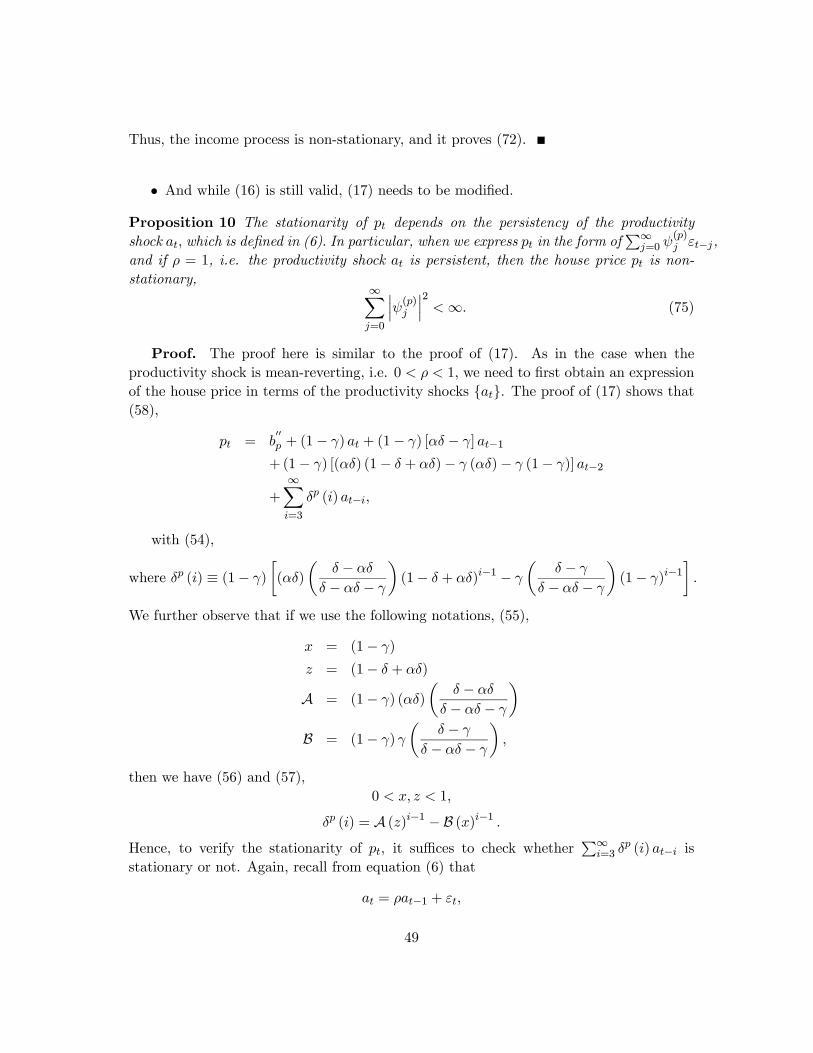
• And while (16) is still valid, (17) needs to be modified.
Proposition 10 The stationarity of depends on the persistency of the productivity
shock which is defined in (6) In particular, when we express in the form ofP∞
=0 () −,
and if = 1, i.e. the productivity shock is persistent, then the house price is non-
stationary,∞X=0
¯̄̄()
¯̄̄2∞ (75)
Proof. The proof here is similar to the proof of (17). As in the case when the
productivity shock is mean-reverting, i.e. 0 1 we need to first obtain an expression
of the house price in terms of the productivity shocks {}. The proof of (17) shows that(58),
= 00 + (1− ) + (1− ) [ − ] −1+(1− ) [() (1− + )− ()− (1− )] −2
+
∞X=3
() −
with (54),
where () ≡ (1− )
∙()
µ −
− −
¶(1− + )−1 −
µ −
− −
¶(1− )−1
¸
We further observe that if we use the following notations, (55),
= (1− )
= (1− + )
A = (1− ) ()
µ −
− −
¶B = (1− )
µ −
− −
then we have (56) and (57),
0 1
() = A ()−1 − B ()−1 Hence, to verify the stationarity of , it suffices to check whether
P∞=3
() − isstationary or not. Again, recall from equation (6) that
= −1 +
49
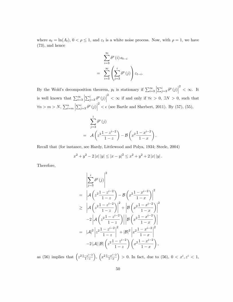
where = ln(), 0 ≤ 1, and is a white noise process. Now, with = 1 we have
(73), and hence
∞X=3
() −
=
∞X=3
⎛⎝ X=3
()
⎞⎠ −
By the Wold’s decomposition theorem, is stationary ifP∞
=3
¯̄̄P=3
()¯̄̄2
∞. Itis well known that
P∞=3
¯̄̄P=3
()¯̄̄2
∞ if and only if ∀ 0, ∃ 0 such that
∀ ,P
=
¯̄̄P=3
()¯̄̄2 (see Bartle and Sherbert, 2011). By (57), (55),
X=3
()
= Aµ21− −2
1−
¶− B
µ21− −2
1−
Recall that (for instance, see Hardy, Littlewood and Polya, 1934; Steele, 2004)
2 + 2 − 2 || || ≤ |− |2 ≤ 2 + 2 + 2 || ||
Therefore, ¯̄̄̄¯̄ X=3
()
¯̄̄̄¯̄2
=
¯̄̄̄Aµ21− −2
1−
¶− B
µ21− −2
1−
¶¯̄̄̄2≥
¯̄̄̄Aµ21− −2
1−
¶¯̄̄̄2+
¯̄̄̄Bµ21− −2
1−
¶¯̄̄̄2−2¯̄̄̄Aµ21− −2
1−
¶¯̄̄̄ ¯̄̄̄Bµ21− −2
1−
¶¯̄̄̄= |A|2
¯̄̄̄21− −2
1−
¯̄̄̄2+ |B|2
¯̄̄̄21− −2
1−
¯̄̄̄2−2 |A| |B|
µ21− −2
1−
¶µ21− −2
1−
as (56) implies that³2 1−
−21−
´,³2 1−
−21−
´ 0 In fact, due to (56), 0 1,
50
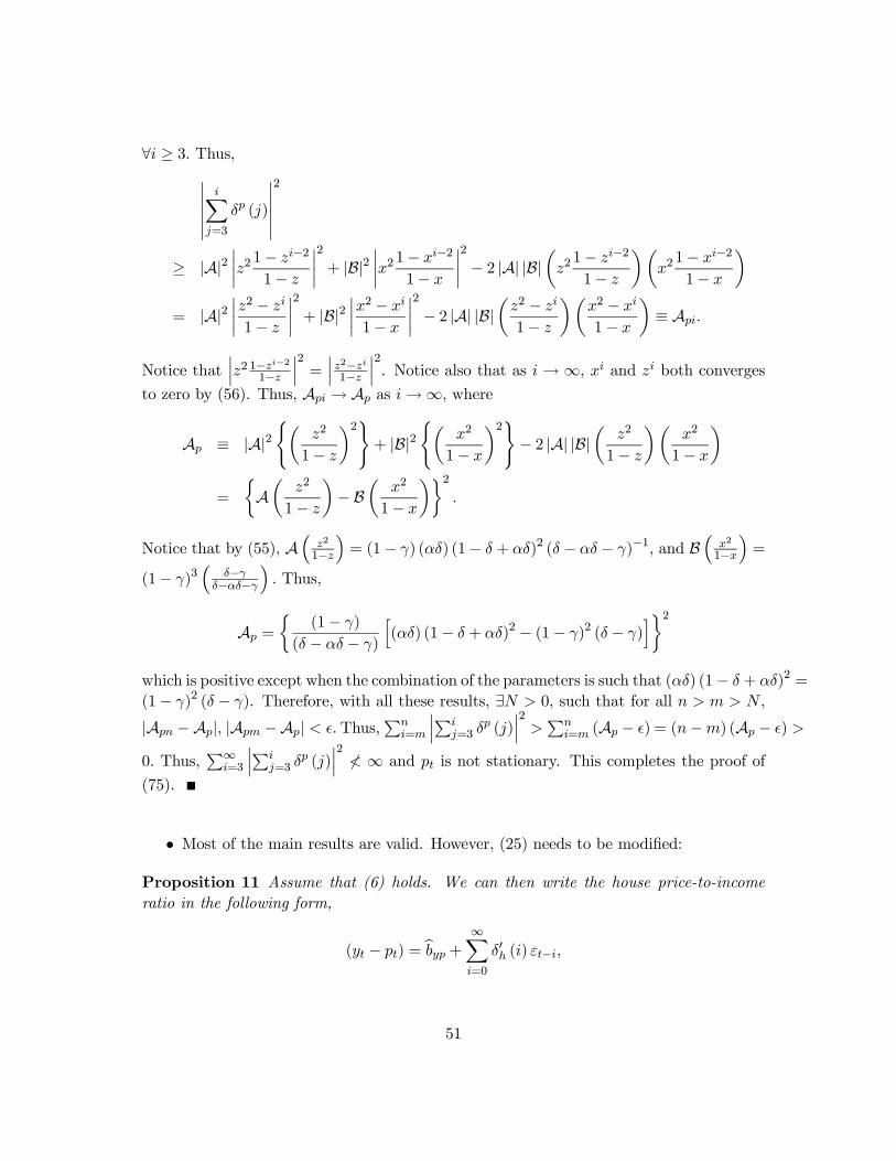
∀ ≥ 3 Thus,¯̄̄̄¯̄ X=3
()
¯̄̄̄¯̄2
≥ |A|2¯̄̄̄21− −2
1−
¯̄̄̄2+ |B|2
¯̄̄̄21− −2
1−
¯̄̄̄2− 2 |A| |B|
µ21− −2
1−
¶µ21− −2
1−
¶= |A|2
¯̄̄̄2 −
1−
¯̄̄̄2+ |B|2
¯̄̄̄2 −
1−
¯̄̄̄2− 2 |A| |B|
µ2 −
1−
¶µ2 −
1−
¶≡ A
Notice that¯̄̄2 1−
−21−
¯̄̄2=¯̄̄2−1−
¯̄̄2. Notice also that as → ∞, and both converges
to zero by (56). Thus, A → A as →∞, where
A ≡ |A|2(µ
2
1−
¶2)+ |B|2
(µ2
1−
¶2)− 2 |A| |B|
µ2
1−
¶µ2
1−
=
½Aµ
2
1−
¶− B
µ2
1−
¶¾2
Notice that by (55), A³
2
1−´= (1− ) () (1− + )2 ( − − )−1, and B
³2
1−´=
(1− )3³
−−−
´ Thus,
A =
½(1− )
( − − )
h() (1− + )2 − (1− )2 ( − )
i¾2which is positive except when the combination of the parameters is such that () (1− + )2 =
(1− )2 ( − ). Therefore, with all these results, ∃ 0, such that for all ,
|A −A|, |A −A| Thus,P
=
¯̄̄P=3
()¯̄̄2P
= (A − ) = (−) (A − )
0 Thus,P∞
=3
¯̄̄P=3
()¯̄̄2≮ ∞ and is not stationary. This completes the proof of
(75).
• Most of the main results are valid. However, (25) needs to be modified:
Proposition 11 Assume that (6) holds. We can then write the house price-to-income
ratio in the following form,
( − ) = b + ∞X=0
0 () −
51
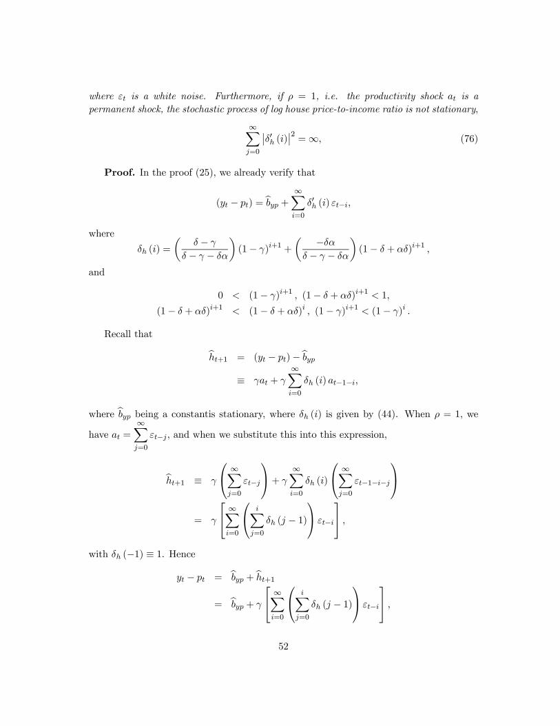
where is a white noise. Furthermore, if = 1, i.e. the productivity shock is a
permanent shock, the stochastic process of log house price-to-income ratio is not stationary
∞X=0
¯̄0 ()
¯̄2=∞ (76)
Proof. In the proof (25), we already verify that
( − ) = b + ∞X=0
0 () −
where
() =
µ −
− −
¶(1− )+1 +
µ − − −
¶(1− + )+1
and
0 (1− )+1 , (1− + )+1 1
(1− + )+1 (1− + ) , (1− )+1 (1− ) .
Recall that
b+1 = ( − )−b≡ +
∞X=0
() −1−
where b being a constantis stationary, where () is given by (44). When = 1 we
have =
∞X=0
− and when we substitute this into this expression,
b+1 ≡
⎛⎝ ∞X=0
−
⎞⎠+
∞X=0
()
⎛⎝ ∞X=0
−1−−
⎞⎠=
⎡⎣ ∞X=0
⎛⎝ X=0
( − 1)⎞⎠ −
⎤⎦ with (−1) ≡ 1. Hence
− = b + b+1= b +
⎡⎣ ∞X=0
⎛⎝ X=0
( − 1)⎞⎠ −
⎤⎦ 52
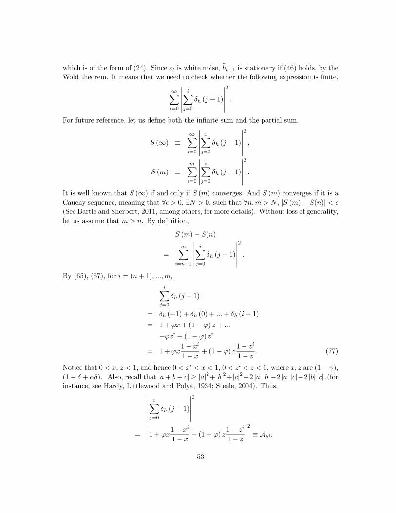
which is of the form of (24). Since is white noise, b+1 is stationary if (46) holds, by theWold theorem. It means that we need to check whether the following expression is finite,
∞X=0
¯̄̄̄¯̄ X=0
( − 1)¯̄̄̄¯̄2
For future reference, let us define both the infinite sum and the partial sum,
(∞) ≡∞X=0
¯̄̄̄¯̄ X=0
( − 1)¯̄̄̄¯̄2
() ≡X=0
¯̄̄̄¯̄ X=0
( − 1)¯̄̄̄¯̄2
It is well known that (∞) if and only if () converges. And () converges if it is a
Cauchy sequence, meaning that ∀ 0, ∃ 0, such that ∀ , | ()− ()|
(See Bartle and Sherbert, 2011, among others, for more details). Without loss of generality,
let us assume that . By definition,
()− ()
=
X=+1
¯̄̄̄¯̄ X=0
( − 1)¯̄̄̄¯̄2
By (65), (67), for = (+ 1) ,
X=0
( − 1)
= (−1) + (0) + + (− 1)= 1 + + (1− ) +
+ + (1− )
= 1 + 1−
1− + (1− )
1−
1− (77)
Notice that 0 , 1, and hence 0 1, 0 1, where are (1− ),
(1− + ). Also, recall that |+ + | ≥ ||2+||2+||2−2 || ||−2 || ||−2 || || (forinstance, see Hardy, Littlewood and Polya, 1934; Steele, 2004). Thus,¯̄̄̄
¯̄ X=0
( − 1)¯̄̄̄¯̄2
=
¯̄̄̄1 +
1−
1− + (1− )
1−
1−
¯̄̄̄2≡ A
53
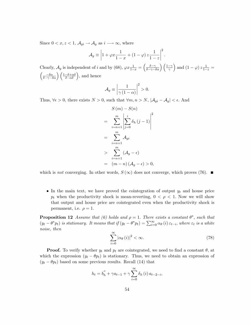
Since 0 1, A → A as −→∞, where
A ≡¯̄̄̄1 +
1
1− + (1− )
1
1−
¯̄̄̄2
Clearly, A is independent of and by (68), 11− =
³−
−−´³
1−
´and (1− ) 1
1− =³−
−−´³
1−+−
´, and hence
A ≡¯̄̄̄
1
(1− )
¯̄̄̄2 0
Thus, ∀ 0, there exists 0, such that ∀ , |A −A| And
()− ()
=
X=+1
¯̄̄̄¯̄ X=0
( − 1)¯̄̄̄¯̄2
=
X=+1
A
X=+1
(A − )
= (− ) (A − ) 0
which is not converging. In other words, (∞) does not converge, which proves (76).
• In the main text, we have proved the cointegration of output and house price when the productivity shock is mean-reverting, 0 1 Now we will show
that output and house price are cointegrated even when the productivity shock is
permanent, i.e. = 1
Proposition 12 Assume that (6) holds and = 1 There exists a constant ∗ such that( − ∗) is stationary. It means that if ( − ∗) =
P∞=0 () − where is a white
noise, then∞X=0
| ()|2 ∞ (78)
Proof. To verify whether and are cointegrated, we need to find a constant , at
which the expression ( − ) is stationary. Thus, we need to obtain an expression of
( − ) based on some previous results. Recall (14) that
= 00 + −1 +
∞X=0
() −2−
54
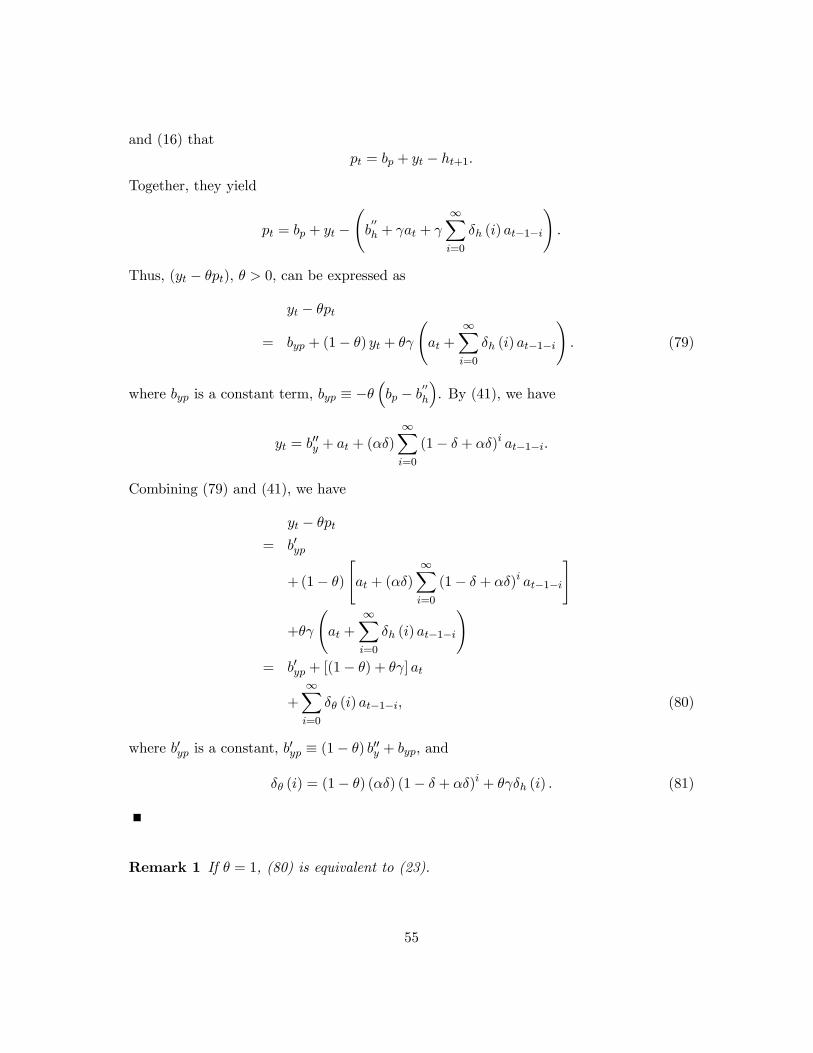
and (16) that
= + − +1
Together, they yield
= + −Ã00 + +
∞X=0
() −1−
!
Thus, ( − ), 0, can be expressed as
−
= + (1− ) +
à +
∞X=0
() −1−
! (79)
where is a constant term, ≡ −³ −
00
´. By (41), we have
= 00 + + ()
∞X=0
(1− + ) −1−
Combining (79) and (41), we have
−
= 0
+(1− )
" + ()
∞X=0
(1− + ) −1−
#
+
à +
∞X=0
() −1−
!= 0 + [(1− ) + ]
+
∞X=0
() −1− (80)
where 0 is a constant, 0 ≡ (1− ) 00 + , and
() = (1− ) () (1− + ) + () (81)
Remark 1 If = 1, (80) is equivalent to (23).
55
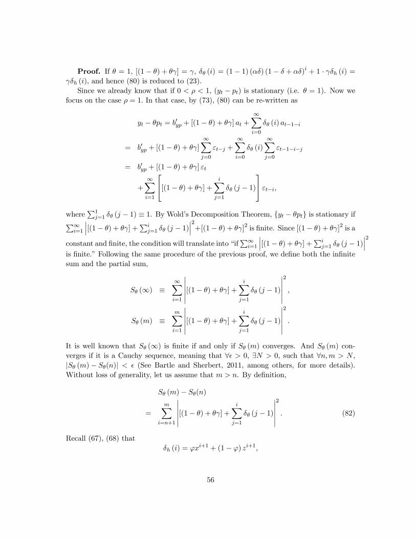
Proof. If = 1, [(1− ) + ] = , () = (1− 1) () (1− + ) + 1 · () = (), and hence (80) is reduced to (23).
Since we already know that if 0 1, ( − ) is stationary (i.e. = 1). Now we
focus on the case = 1 In that case, by (73), (80) can be re-written as
− = 0 + [(1− ) + ] +
∞X=0
() −1−
= 0 + [(1− ) + ]
∞X=0
− +∞X=0
()
∞X=0
−1−−
= 0 + [(1− ) + ]
+
∞X=1
⎡⎣[(1− ) + ] +
X=1
( − 1)⎤⎦ −
whereP1
=1 ( − 1) ≡ 1. By Wold’s Decomposition Theorem, { − } is stationary ifP∞=1
¯̄̄[(1− ) + ] +
P=1 ( − 1)
¯̄̄2+[(1− ) + ]2 is finite. Since [(1− ) + ]2 is a
constant and finite, the condition will translate into “ifP∞
=1
¯̄̄[(1− ) + ] +
P=1 ( − 1)
¯̄̄2is finite.” Following the same procedure of the previous proof, we define both the infinite
sum and the partial sum,
(∞) ≡∞X=1
¯̄̄̄¯̄[(1− ) + ] +
X=1
( − 1)¯̄̄̄¯̄2
() ≡X=1
¯̄̄̄¯̄[(1− ) + ] +
X=1
( − 1)¯̄̄̄¯̄2
It is well known that (∞) is finite if and only if () converges. And () con-
verges if it is a Cauchy sequence, meaning that ∀ 0, ∃ 0, such that ∀ ,
| ()− ()| (See Bartle and Sherbert, 2011, among others, for more details).
Without loss of generality, let us assume that . By definition,
()− ()
=
X=+1
¯̄̄̄¯̄[(1− ) + ] +
X=1
( − 1)¯̄̄̄¯̄2
(82)
Recall (67), (68) that
() = +1 + (1− ) +1
56
where
=
µ −
− −
¶ = (1− ) 0
= (1− + ) 0
Thus, (81) can be re-written as
() = (1− ) () (1− + ) + ()
= (1− ) () + £+1 + (1− ) +1
¤
and we can re-write (82),
()− () =
X=+1
||2 (83)
where is defined as the following,
≡ [(1− ) + ] +
X=1
( − 1)
= [(1− ) + ]
+ (1− ) () + [+ (1− ) ]
+ (1− ) () + £2 + (1− ) 2
¤+
+(1− ) () −1 + £ + (1− )
¤= [(1− ) + ] + (1− ) ()
1−
1−
+
∙1−
1− + (1− )
1−
1−
¸= [(1− ) + ] +
∙1−
1−
¸+ [(1− ) () + (1− ) ]
µ1−
1−
57
Notice that can be re-written as
= [(1− ) + ] +
∙1−
1−
¸+ [(1− ) () + (1− ) ]
µ1−
1−
¶= [(1− ) + ] +
∙
1
1−
¸+ [(1− ) () + (1− ) ]
µ1
1−
¶−½
∙
1−
¸+ [(1− ) () + (1− ) ]
µ
1−
¶¾ (84)
Intuitively, if
[(1− ) + ] +
∙
1
1−
¸+ [(1− ) () + (1− ) ]
µ1
1−
¶= 0 (85)
then will be significantly simplified,
= −½
∙
1−
¸+ [(1− ) () + (1− ) ]
µ
1−
¶¾and since 0 1, → 0 as →∞ and hence → 0. Thus, we need to choose
such that (85) holds. Clearly, (85) holds if and only ifµ1 +
()
1−
¶=
½µ1 +
()
1−
¶−
∙(1− )
1− +
1−
¸¾ (86)
By (68),
1− =
1−
1
1− =
1
(1− )
1− =
1− (1− )
(1− )
=
µ −
− −
which means that (86) can be further simplified as
1
1− =
½µ1
1−
¶−
∙µ −1−
¶µ1− (1− )
− −
¶+
µ −
− −
¶µ1−
¶¸¾=
½2 + + − − 2(1− ) ( − − )
¾ (87)
58

Since 0 1, (87) implies that
=( − − )
2 + − + ( − − )
=1
1− (88)
As 0 1, 1. Also, since = 11− , 1− = −
1− = −Observe further that as (85) holds, (84) can be simplified as
= −½
∙
1−
¸+ [(1− ) () + (1− ) ]
µ
1−
¶¾= D1 +D2 (89)
where
D1 ≡ −
1−
=
µ1−
1−
¶µ −
− −
D2 ≡ − [(1− ) () + (1− ) ]1
1−
=−
(1− )2
∙+
µ1− +
− −
¶¸
and hence both D1 and D2 are constant. For future reference, let us define
= max { }
Since 0 1, 0 1 Hence,
0 () ()
1, ∀ 1 (90)
Similarly, define
= max {|D1| , |D2|} Now combine (89) with (83), and follow Hardy, Littlewood and Polya (1934), Steele (2004),
59
we have
()− ()
=
X=+1
||2
=
X=+1
¯̄D1 +D2
¯̄2=
X=+1
¯̄̄¡D1
¢2+¡D2
¢2+ 2
¡D1
¢ ¡D2
¢¯̄̄
X=+1
n¯̄
¯̄2+¯̄
¯̄2+ 2
¡¢ ¡¢ |D1| |D2|o
||2X
=+1
¯̄ +
¯̄2≤ ||2
X=+1
¯̄̄2 ()
¯̄̄2
=
X=+1
()2
where
≡ 4 ||2 Therefore, ∀ 0, ∀ ,
()− ()
≤
X=+1
()2
∞X=+1
()2 as 0 1
=
µ1
1− ()2¶()
2(+1)
µ1
1− ()2¶()
2(+1) as 0 1
Now define
≡
µ1
1− ()2
60
And since 0 1, ln 0. Thus, | ()− ()| ()2(+1) ,
if 1
2
Ãln¡
¢ln
!− 1
Thus, () converges and hence ( − ) is stationary.
C More Discussion on and
Throughout the paper, the relative magnitude of two parameters, and are of great
importance. For instance, in the previous proof,
() = (1− )+1 + ()
X=0
(1− )− (1− + )
= (1− )+1 + ()(1− )+1 − (1− + )+1
− −
= (1− )+1µ
−
− −
¶+ (1− + )+1
µ − − −
Thus, we can interpret () as a “weighted average” of two terms, (1− )+1 and
(1− + )+1 Furthermore, since and are strictly between 0 and 1, 0 (1− + ) =
(1− (1− )) 1. Therefore, 0 (1− + )+1 (1− + ) 1, = 0, 1, 2,....
Similarly, since 0 1, 0 (1− ) 1. Therefore, we also have 0 (1− )+1
(1− ) 1.
How about the “weights,” i.e.³
−−−
´and
³−
−−´? Clearly, if ( − − ) 0,³
−−−
´ 1 and
³−
−−´ 0 In the macroeconomic literature, the capital share of
output, has been estimated many times and it is typically around 03 to 035 (Cooley,
1995). For simplicity, let us assume that = 13 On the other hand, empirical estimates
for the parameters and are quite different that it may affect how we proceed. Let us
take a few examples to illustrate.
1. According to Greenwood and Hercowitz (1991), = = 0078 on quarterly basis.
In that case, − = 0 and hence
() = (1− + )+1
which is clearly a converging sequence as 0 (1− + ) 1
61
2. According to Davis and Heathcote (2005), = 0056, = 0016 on quarterly basis.
In that case, − = 004, − − = 0056− 0016− (0056) ∗ (13) = 002 1 0Hence
() ≈ 2 (1− )+1 − (1− + )+1
From this point on, we impose the following assumption,
≥ 0 (91)
for future reference.
On the other hand, while both previous studies and causal observations support (91),
we do not know in general whether ( − − ) 0 or not. Notice that
( − − ) 0
⇔ (1− )
⇔ (1− )
(92)
The left hand side of the last expression is the labor share, or unity minus the capital
share. The right hand side of the same expression is the ratio of the depreciation rate of
residential housing relative to the depreciation rate of business capital. Thus, equation
(92) comapres the relative magnitude of two forces. One is the share of factors (which is
labor in this model) other than business capital. The second force is the relative speed
of business capital depreciation relative to the counterpart of another stock (which is
residential housing in this model). Theoretically, there is no clear reason of why one
should dominate the other. Since we cannot be sure whether ( − − ) 0 or not, we
cannot be sure whether³
−−−
´is larger than unity or not.
In terms of the dynamics of (), we can actually say a few more words. Notice that
(+ ) ()
= (+ )¡+1 + (1− ) +1
¢= +2 + (1− ) +1+ +1 + (1− ) +2
= (+ 1) + ¡(1− ) +
¢= (+ 1) + (− 1)
We re-state the result in the following lemma.
Lemma 3 () evolves according to the following formula,
(+ 1) = (+ ) ()− · (− 1) (93)
Notice that for empirically plausible parameterization, (+ ) = (1− )+(1− + )
1 whereas = (1− ) · (1− + ) hence 0 1.
62