Embed Size (px)
Citation preview

au s t r a l i an aac t u a r i a l j o u r n a l 22012 Volume 18 Issue 1 pp. 67-80
667
�
Act
uarie
s In
stitu
te o
f A
ustr
alia
201
2
Error in Joint Mortality Formulas
M Boggess & M Moyer*
Abstract
Life Contingencies is the study of probability and the time value of money whose objective is the valuation of quantities associated with life insurance and annuities. Since policies on a husband and wife are common, actuarial exams covering life contingencies include the situation where the lifetimes of the husband and wife are dependent and the policy payout depends on the time of the first or second death. We show that some well-known formulas are incorrect, and whose application by the Society of Actuaries in their solutions to exam questions has led to incorrect answers. These formulas can be rectified by the inclusion of notation that makes specific the necessary conditioning events.
Keywords: life contingencies; joint mortality formula error
* Contact : May M Boggess, B.Math.(Hons I) M.Sc.(Stat). PhD, Associate Professor,School of Mathemat ical and Stat ist ical Sciences, Arizona State University,[email protected] Moyer, B.Sc.(Applied Math) M.Sc.(Math), Actuarial Analyst II, USAA, San Antonio TX, USA, [email protected].
Enfocus Software - Customer Support

au s t r a l i an aac t u a r i a l j o u r n a l
668
�
Act
uarie
s In
stitu
te o
f A
ustr
alia
201
2
1 Introduction
In 2002 Youn, Shemyakin and Herman [12] claimed that standard actuarial formulas, Equations (1), (3) and (4) below, are not always correct. James Hickman and Donald Jones [4] responded that, while there are some issues, it is just a “notational deficiency”. In his response, S. David Promislow [9] acknowledged there is a problem arising when modelling joint lives with dependency other than common shock, including models on real data [3]. However, rather than supporting Youn, Shemyakin and Herman's call for a notational fix to the problem, Promislow asserted that “anyone sophisticated enough to use the copula model in the first place ... would be aware of the need to change the marginal” [9, p.115]. In the event that one inadvertently applied the formulas, he claimed (without supporting detail) that the size of pricing errors caused would be negligible in practice [12, p. 167]. But Youn, Shemyakin and Herman had used a copula model estimated on data of joint and last-survivor annuity contracts containing 11,457 married couples from a large Canadian company [11] and showed that the formulas would result in an error in the last-survivor actuarial present value of approximately 10%. It is time for this debate to be resolved.
Here we confirm that errors nearing 10% are possible in practice and show that the use of Equations (1) to (5) has led to incorrect answers on the U.S. Society of Actuaries (SOA) Life Contingencies (MLC) Exam [10]. All members of the actuarial profession have reason to be concerned when it is shown that an exam question did not have an unambiguous correct answer, and when misleading formulas may result in errors large enough to cause financial loss.
We begin with definitions of standard actuarial notation from
Bowers et. al. [1, Chapter 3]. Let X and Y be random variables
representing age at death. Let T(x) be the future lifetime for (x) a
person aged x, T(xy) be the future lifetime for (xy) the minimum of
two future lifetimes, and ( )T xy be the future lifetime for ( )xy the
maximum:
Enfocus Software - Customer Support

Error in Joint Mortality Formulas
669
�
Act
uarie
s In
stitu
te o
f A
ustr
alia
201
2
� � � �, ,T x X x X x T y Y y Y y� � � �
( ) min{ ( ), ( )} min{ – , – } | , ,T xy T x T y X x Y y X x Y y� � and
( ) max{ ( ), ( )} max{ – , – } | , .T xy T x T y X x Y y X x Y y� �
The probability that a person aged (x) will live t more years is denoted by
( ( ) ) ( | ),t xp P T x t P X x t X x� � �
so that
� �� � � �or | , ,t xyp P T xy t P X x t Y y t X x Y y� � � - - �
and
� � � �( ) or | , .t xyp P T xy t P X x t Y y t X x Y y� � � - �
The following joint mortality functions are derived in Bowers et. al.:
,t xy t xy t x t yp p p p� � � (1)
,xyxy x ye e e e� � � (2)
,xy xy x yA A A A� � � (3)
,xy xy x ya a a a� � � (4)
+ ,xy xy x ya a a a� ��� �� �� �� (5)
the first of which is equivalent to � � � � � �( ) ( ) ( ) ( ) ( )T xy T xy T x T yF t F t F t F t� � �
[1, pages 268, 272, 282], [2, pages 265, 266, 286]. To get to the root of
the problem, the conditioning events need to be carefully followed:
� � � �( ) ( )T xy T xyF t F t�
. /� �min , | ,P X x Y y t X x Y y� � � !
. /(max , | , )P X x Y y t X x Y y� � � !
� � � �, | , | ,P X x t Y y t X x Y y P X x t Y y t X x Y y� � ! � ! � � ! 0 � ! ( , ) ( , )
( , ) ( , )P x X x t y Y y t P x X x t Y y
P X x Y y P X x Y y! ! � ! ! � ! ! �
� �
Enfocus Software - Customer Support
au s t r a l i an aac t u a r i a l j o u r n a l
770
�
Act
uarie
s In
stitu
te o
f A
ustr
alia
201
2
( , ) ( , )
( , ) ( , )P y Y y t X x P x X x t y Y y tP X x Y y P X x Y y! ! � ! ! � ! ! �
� �
( , ) ( , )( , ) ( , )
P x X x t Y y P y Y y t X xP X x Y y P X x Y y! ! � ! ! �
� �
� � � �| , | ,P X x t X x Y y P Y y t X x Y y� � ! � � ! ,
which may differ from:
� � � � � � � � � � � �| |T x T yF t F t P X x t X x P Y y t Y y� � � ! � � !
if X and Y are not independent. Hickman, Jones and Promislow's
responses to Youn, Shemyakin and Herman included the assertion
that the size of the error obtained when using Equation (3) is
negligible for practical purposes. This assertion was based on
calculations for which no supporting detail was provided. Thus we
begin with the calculations involved in their example, which we
performed in MapleTM
2 Youn, Shemyakin and Herman, Example 2
[7] (code available from corresponding author).
Youn, Shemyakin and Herman chose Weibull marginal
distributions, � � ( / )( / )1mx mF x e��� � and Hougaard's copula
[8, page 96] � � � �1/, exp [( ln ) ( ln ) ] ,C u v u v� � �� � � � � with 1.638� � [12,
Example 2]. Thus, the joint cumulative distribution function is
� � � �9.96 7.65 0.613.02 1.64 3.18 1.64, exp [ ln(1 )] [ ln(1 )] ,x yH x y e e� �� �� � � � � � �� �
� �
with 0.8951,xm � 8.99,x� � 0.8598,ym � and 11.24y� � (where ,xm,ym x and y have been scaled by 100). Let ( )a
xF t be the conditional
cumulative distribution function for the continuous lifetime random
variable |X a X a� :
( , ) ( , ) .1 (
),
()a
x H a t H aFH a
t � 1 � 1�
� 1
Following Youn, Shemyakin and Herman, x = 0.65 and y = 0.7:
Enfocus Software - Customer Support

Error in Joint Mortality Formulas
771
�
Act
uarie
s In
stitu
te o
f A
ustr
alia
201
2
� � � �9.96 1.6465
0.613.02(0.65 )1.042e )xp [ ]ln(1 0.042,x tF t e� �� �� � � � �� �
� �
� � � �7.65
70
0.613.18(0.7 ) 1.64[ )]1.231exp ln(1 0.231.x tF t e� �� �� � � �� �
��
�
The actuarial present value of a payment of one dollar made to a person currently aged (x) at the time of death is
0 0
( ) ( )rt rtx x xA e f dt re F tt dt
1 1� �� �2 2
[1, 4.2.6, page 96]. Using r = 0.05, 565 65
0
(5 0.382176238) 4x t xA e F dtt1
�� �2
and 70 0.5098231502.yA � The conditional cumulative distribution
function of the maximum is
� � � � � �� � � �
0.65 ,0.7 0.65 ,0.7 0.65,0.7 (0.65,0.7)( ) .
1 0.65, ,0.7 (0.65,0.7)xy
H t t H t H t HF t
H H H� � � � � � �
�� 1 � 1 �
Since � �H 0.65,0.7 =0.02141613958, � �0.65, 0.04046117300H 1 � and
� �,0.7 0.1873252219,H 1 � the denominator is 0.7936297447. The
numerator has three parts that are functions of t:
� �7.65 0.6113.18(0.7 ) 1.64(0.65,0.7 ) exp ln(1 6.746 ,[ )] 5tH t e� �� �� � � � � �� �
� �
� �9.96 0.6113.02(0.65 ) 1.64(0.65 ,0.7) exp ln(1 2. 2)] 3 8[ ,tH t e� �� �� � � � � �� �
� �
� �
� � � �9.96 7.651.64
0.613.02 0.65 3.18 0.71.64
0.65 ,0.7
exp ln(1 l[ )] [ )n .](1t t
H t t
e e� � � ��
� �
� �� �� � � � � �� �� �� �� �� �
Enfocus Software - Customer Support
au s t r a l i an aac t u a r i a l j o u r n a l
772
�
Act
uarie
s In
stitu
te o
f A
ustr
alia
201
2
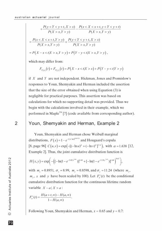
The actuarial present value is then 0.3335436046.xyA � The integral
was evaluated in MapleTM
� � � � � �� � � �
1 0.65 , ,0.7 0.65 ,0.71 .
1 0.65, ,0.7 (0.65, .( )
0 7)xy
H t H t H t tH H H
tF� � 1 � 1 � � � �
� �� 1 � 1 �
using Simpson's rule with 10,000 partitions
between t = 0 and t = 30, and by comparison with larger and smaller
domains with more and less partitions, this answer is accurate to at
least seven decimal places. The conditional cumulative distribution
function of the minimum is
The numerator has the following components that are functions of t:
� �7.65 0.613.18(0.7 ) 1.64[( ,0.7 ) exp ln(1 ] ,)tH t e� �� �1 � � � � �� �
� �
� � � �9.96 0.613.016 0.65 1.640.65 , exp ln[ )](1 .tH t e� �� �� �� 1 � � � �� �� �� �� �� �
The actuarial present value is then 0.5292504872.xyA � Using
Equation (3)
65 70 65:7065:70
0.3821762384 0.5098231502 0.52925048720.3627495096,
x yA A A A� � �
� � ��
whereas the correct value is 0.3335436046,xyA � a percentage error of
8.8%, which is in close agreement with Youn, Shemyakin and
Herman's original calculations.
3 Errors in SOA Sample Exam Questions
3.1 Course 3, May 2001, Question 9
This question is also in the Society of Actuaries MLC Exam
sample questions [10, Q104]: (x) and (y) are two lives with identical
expected mortality. You are given: 0.1, 0.06,x y xyP P P� � � xyP is the
annual benefit premium for a fully discrete insurance of 1 on (xy) and
Enfocus Software - Customer Support

Error in Joint Mortality Formulas
773
�
Act
uarie
s In
stitu
te o
f A
ustr
alia
201
2
d = 0.06. Calculate the premium ,xyP the annual benefit premium for a
fully discrete insurance of 1 on (xy).
For this example we choose geometric marginal distributions for
both X and Y, � � 11 (1 ) ,kF k p �� � � where 0,1,2,3,k � 3 and
0.84
0.941 .p � � Frank's copula is used [6, 3.45, page 112],
� � 1 ( 1)( 1), ln 1 ,1
u ve eC u ve
� �
��� �� �
� �� ��� �
with 1.89876941.� � Then the joint cumulative distribution function is
� � � � � �� �111.899 1.899 0.894 1.899 1.899 0.894, 0.5267ln 1 1.177( 1)( 1) .yx
H x y e e��� � � �� � � � �
Take (x) = 1 and (y) = 1, meaning, the given event is X>0 and Y>0.
The conditional marginal cumulative distribution function is
� �� �
0,(
0)x
P XF
Xk
kP!
�
so that 0.841 .0.94
( )x
k
F k � �� � � �� �
Since d = 0.06, the
annual discounting factor is v = 0.94 and the actuarial present value of
a payment of one dollar made to a person currently aged (x) at start
of each year prior to death is
� �0
11 6.2516
( )kx x
k
v Fa k1
�
� � � ����
[1, 5.2.4, page 135]. The level annual benefit premium is valued at
0.11x xaP d� � ��� [1, 6.3.2, page 180], and similarly for Y. The
conditional cumulative distribution function of the maximum is
� � � � � �� � � �
, ,0 0, (0,0)( .
1 0, ,0 (0, ))
0xy
H t t H t H t HF
H H Ht
� � ��
� 1 � 1 �
The denominator is 1 - 2(0.1063829789) + 0.02114017770 = 0.8083742199. The numerator has the following components that are functions of t:
Enfocus Software - Customer Support
au s t r a l i an aac t u a r i a l j o u r n a l
774
�
Act
uarie
s In
stitu
te o
f A
ustr
alia
201
2
� � � �� �11.899 1.899 0.89360.2020, 0.5267ln 1 1.176( 1)( 1) ,t
H t e e�� ��� � � � �
� � � � 121.899 1.899 0.8936, 0.5267ln(1 1.176( 1 .))
tH t t e
�� �� � � �
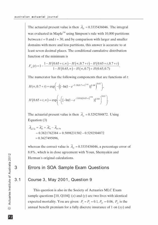
The conditional cumulative distribution function of the minimum is
� � � � � �� � � �
1 , , ( , )1 .
1 0, ,0 (0,0)xy
H t H t H t tF t
H H H� 1 � 1 �
� �� 1 � 1 �
The numerator has the following components that are functions of t:
� � � �0.1125 0.11251.899 1.899, 0.5267ln .teH t e
� �� �1 � �
Then 8.333,xya ��� 0.06,xyP � 4.50456103xya ��� and 0.161997211.xyP � A
different answer is obtained by using Equation (5):
4.167xy y xx ya a aa � � � ���� �� ��� and 0.179981.xyP �
The SOA answer is (C) 0.18 using Equation (4), whereas by direct
calculation, we see that the correct answer is (B) 0.16 in this instance.
3.2 Course 3, May 2001, Question 23
This question is also in the Society of Actuaries MLC Exam sample questions [10, Q112]: A continuous two-life annuity pays: 100 while both (30) and (40) are alive; 70 while (30) is alive but (40) is dead; and 50 while (40) is alive but (30) is dead. The actuarial present value of this annuity is 1180. Continuous single life annuities paying 100 per year are available for (30) and (40) with actuarial present values of 1200 and 1000, respectively. Calculate the actuarial present value of a two-life continuous annuity that pays 100 while at least one of them is alive.
Consider the following bivariate exponential distribution [5, page 352] with joint cumulative distribution function
� � ( )( )., 1 y x y x yx y x y x yxH x y e e e� � � � � �� � � � ��� � � �
Enfocus Software - Customer Support
Error in Joint Mortality Formulas
775
�
Act
uarie
s In
stitu
te o
f A
ustr
alia
201
2
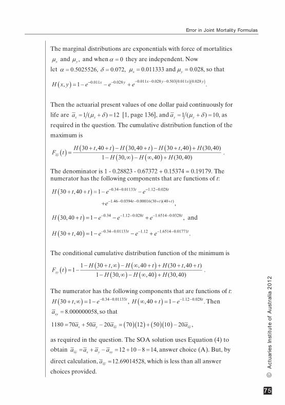
The marginal distributions are exponentials with force of mortalities
x� and ,y� and when 0� � they are independent. Now
let 0.5025526,� � 0.072,4 � 0.011333x� � and 0.028,y� � so that
� � � �� �0.011 0.028 0.503 0.011 0.0280.0280.011, 1 .x y x yyxH x y e e e� � ���� � � �
Then the actuarial present values of one dollar paid continuously for
life are 1 ( ) 12x xa � 4� � � [1, page 136], and 1 ( ) 10,y ya � 4� � � as
required in the question. The cumulative distribution function of the
maximum is
� � � � � � � �� � � �
30 ,40 30,40 30 ,40 (30,40).
1 30, ,40 (30,40)xy
H t t H t H t HF t
H H H� � � � � � �
�� 1 � 1 �
The denominator is 1 - 0.28823 - 0.67372 + 0.15374 = 0.19179. The numerator has the following components that are functions of t:
� � 0.34 0.01133 1.12 0.02830 ,40 1 t tH t t e e� � � �� � � � �
1.46 0.0394 0.00016(30 )(40 ) ,t t te� � � � ��
� � 0.34 1.12 0.028 1.6514 0.032830,40 1 ,t tH t e e e� � � � �� � � � � and
� � 0.34 0.01133 1.12 1.6514 0.0177130 ,40 1 .t tH t e e e� � � � �� � � � �
The conditional cumulative distribution function of the minimum is
� � � � � �� � � �
1 30 , ,40 (30 ,40 )1 .
1 30, ,40 (30,40)xy
H t H t H t tF t
H H H� � 1 � 1 � � � �
� �� 1 � 1 �
The numerator has the following components that are functions of t:
� � 0.34 0.0113330 , 1 ,tH t e� �� 1 � � � � 1.12 0.028,40 1 .tH t e� �1 � � � Then
8.000000058,xya � so that
� �� � � �� �1180 70 50 20 70 12 50 1 0 ,0 2xx y y xya a a a� � � � � �
as required in the question. The SOA solution uses Equation (4) to
obtain 12 10 8 14,x y xyxya a a a� � � � � � � answer choice (A). But, by
direct calculation, 12.69014528,xya � which is less than all answer
choices provided.
Enfocus Software - Customer Support
au s t r a l i an aac t u a r i a l j o u r n a l
776
�
Act
uarie
s In
stitu
te o
f A
ustr
alia
201
2
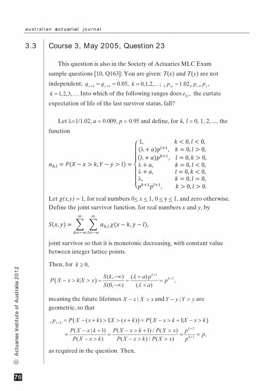
3.3 Course 3, May 2005, Question 23
This question is also in the Society of Actuaries MLC Exam
sample questions [10, Q163]: You are given: T(x) and T(y) are not
independent; 0.05,x k y kq q� �� � 0,1,2, ;k � 3 1.02 ,k xy k x k yp p p�
1,2,3, .k � 3 Into which of the following ranges does ,xye the curtate
expectation of life of the last survivor status, fall?
Let 5=1/1.02, a = 0.009, p = 0.95 and define, for k, l = 0, 1, 2, ..., the
function
��,� = �(� � � > �, � � � > ) =!""#""$ 1, � < 0, < 0,(5+ &)'��*, � = 0, > 0,(5 + &)'��*, = 0, � > 0,5 + &, � = 0, < 0,5 + &, = 0, � < 0,5, � = 0, = 0,'��*'��*, � > 0, > 0.
-
Let /(x,y) = 1, for real numbers 0< x < 1, 0 < y < 1, and zero otherwise. Define the joint survivor function, for real numbers x and y, by
2(�, �) = 3 3 ��,�4
�5644
�564/(� � �, � � ),
joint survivor so that it is monotonic decreasing, with constant value between integer lattice points.
Then, for 0,k "
� �1
1( , ) ( )| ,(0, ) ( )
kkS k a pP X x k X x p
S a55
���1 �
� � � ��1 �
meaning the future lifetimes |X x X x� and |Y y Y y� are geometric, so that
� � � �1
2
1
( ) 1| ( ) 1|
( | 1) ( 1) / ( ) ,( ) ( ) / ( )
x k
k
k
p P X x k X x k P X x k X x k
P X x k P X x k P X x p pP X x k P X x k P X x p
�
�
�
� � � � � � � �
� � � � � � � �
� �
as required in the question. Then,
Enfocus Software - Customer Support
Error in Joint Mortality Formulas
777
�
Act
uarie
s In
stitu
te o
f A
ustr
alia
201
2
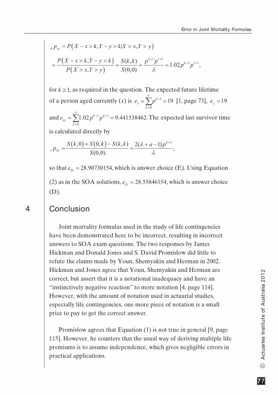
� �, | ,k xyp P X x k Y y k X x Y y� � �
� �� �
1 11 1, ( , ) 1.02 ,
, (0,0)
k lk lP X x k Y y k S k k p p p p
P X x Y y S 5
� �� �� �
� � � �
for 1,k " as required in the question. The expected future lifetime
of a person aged currently (x) is 1
0
19kx
k
e p1
�
�
� �� [1, page 73], 19ye �
and 1 1
0
1.02 9.441538462.k kxy
k
e p p1
� �
�
� �� The expected last survivor time
is calculated directly by
� � � � 1,0 0, ( , ) 2( 1) ,(0,0)
k
t xy
S k S k S k k a ppS
55
�� � � �� �
so that 28.90730154,xye � which is answer choice (E). Using Equation
(2) as in the SOA solutions, 28.55846154,xye � which is answer choice
(D).
4 Conclusion
Joint mortality formulas used in the study of life contingencies have been demonstrated here to be incorrect, resulting in incorrect answers to SOA exam questions. The two responses by James Hickman and Donald Jones and S. David Promislow did little to refute the claims made by Youn, Shemyakin and Herman in 2002. Hickman and Jones agree that Youn, Shemyakin and Herman are correct, but assert that it is a notational inadequacy and have an “instinctively negative reaction” to more notation [4, page 114]. However, with the amount of notation used in actuarial studies, especially life contingencies, one more piece of notation is a small price to pay to get the correct answer.
Promislow agrees that Equation (1) is not true in general [9, page 115]. However, he counters that the usual way of deriving multiple life premiums is to assume independence, which gives negligible errors in practical applications.
Enfocus Software - Customer Support

au s t r a l i an aac t u a r i a l j o u r n a l
778
�
Act
uarie
s In
stitu
te o
f A
ustr
alia
201
2
We believe it is fundamentally wrong to assume independence when it is not true, and this is an inadequate way to deal with this problem, particularly for SOA exams. We put forth two suggestions based on this work:
1. Since � �| , ( | )P X x t X x Y y P X x t X x� � � in common
shock models, SOA examiners could utilise these joint distributions and thereby avoid any possible ambiguity in the answer choices.
2. Youn, Shemyakin and Herman suggest that notation be included on t xp to indicate the additional conditioning on y as follows:
� �|| | , .t x yp P X x y X x Y y� �
Then formulas such as
|| || ,t xy t xy t x y t y xp p p p� � �
can be applied accurately. Based on the inaccuracies in the Society of Actuaries exams shown here, we suggest that Youn, Shemyakin and Herman's notation be adopted by actuarial students and practitioners alike.
Enfocus Software - Customer Support

Error in Joint Mortality Formulas
779
�
Act
uarie
s In
stitu
te o
f A
ustr
alia
201
2
References
[1] Bowers, N, Gerber, H, Hickman, J, Jones, D, & Nesbitt, C (1986). Actuarial Mathematics. Society of Actuaries, Itasca, IL
[2] Dickson, D, Hardy, M & Waters, H (2009). Actuarial Mathematics for Life Contingencies. Cambridge University Press, Cambridge, UK
[3] Frees, E, Carriere, J & Valdez, E (1996). Annuity evaluation with dependent mortality. Journal of Risk and Insurance, 63(2):229-261
[4] Hickman, J & Jones, D (2002). Response to “A re-examination of the joint mortality functions”. North American Actuarial Journal, 6(4):113-114
[5] Kotz, S, Johnson, NL & Balakrishnan, N (2000). Continuous Multivariate Distributions: Models and applications. John Wiley and Sons, New York, NY
[6] Malevergne, Y & Sornette, D (2005). Extreme Financial Risks: From Dependence to Risk Management. Springer, New York, NY
[7] Maplesoft (2008). Maple 12. Waterloo ON, Canada
[8] Nelsen, R (2009). An Introduction to Copulas. Springer, New York, NY
[9] David Promislow, S (2002). Response to “A re-examination of the joint mortality functions”. North American Actuarial Journal, 6(4):114-117
Enfocus Software - Customer Support

au s t r a l i an aac t u a r i a l j o u r n a l
880
�
Act
uarie
s In
stitu
te o
f A
ustr
alia
201
2
[10] Society of Actuaries (April 2010). Exam M, Actuarial Models, Life Contingencies Segment (MLC). http://www.soa.org/files/pdf/edu-2008-spring-mlc-questions.pdf
[11] Youn, H & Shemyakin A (August 1999). Statistical aspects of joint life insurance pricing. In 1998 Proceedings of the Business and Economic Statistics Section, American Statistical Association Meeting, Dallas, TX, pages 34-38
[12] Youn, H & Shemyakin A & Herman, E (2002). A re-examination of the joint mortality functions. North American Actuarial Journal, 6(1):166-170
Enfocus Software - Customer Support
![{]tXy-I-hn-`m-K-ß-fpsS {Kma-k`dspace.kila.ac.in:8080/jspui/bitstream/123456789/57... · ssI∏p-kvXIw 2 {]tXy-I-hn-`m-K-ß-fpsS {Kma-k` 2 Ah-Xm-cnI P\-߃°v `cW˛hnI-k\ Imcy-ß-fn¬](https://img.pdfslide.net/doc/110x75/607edfc7e362e53f7768bbc3/txy-i-hn-m-k-fpss-kma-k-ssiap-kvxiw-2-txy-i-hn-m-k-fpss-kma-k.jpg)


![4>9G@AE 4EB86FAE BE;6A>A9;6AE - DialnetR_\TOLO TXO_]^\TLV XY P] NY]^Y ]TXY TX`P\]TYX& VL ]PR_\TOLO LQPN(^T`L ^LWMTPX \PO_XOL PX )MPXPQTPTY] ZL\L PV SYWM\P c VL TXO_](^\TL) 8] P]^P](https://img.pdfslide.net/doc/110x75/5ffeb80480455915753e7339/49gae-4eb86fae-be6aa96ae-dialnet-rtolo-txotlv-xy-p-nyy-txy.jpg)


![-„-s∏-Sp-∂p...PUBLISHED FROM THIRUVALLA ON 05-07-2014 hmeyw ˛ 9 e w: 7 Pqsse 2014 Annual Subscription RS. 100/- KERMAL / 2007 / 21096 {]-tXy-I te-J-I≥ tI-c-f-Øn-se ap-Jy-[m-cm](https://img.pdfslide.net/doc/110x75/5f0c5f8f7e708231d4351471/-a-sa-sp-ap-published-from-thiruvalla-on-05-07-2014-hmeyw-9-e-w-7.jpg)
![WL ]T' · 2014-06-30 · zl\l [_p op] op lvvt vp] op ]_ \p]zpn^t`y op]^txy% px vl qy\wl ]t' r_tpx^p4 cl\l px^\prl\ lv 9awy( fpxy\ 7yxop op vl 7lxlol% nywy ;ymp\xloy\ opv ekplvv b](https://img.pdfslide.net/doc/110x75/5e577e6bc325a3759f29d0c7/wl-t-2014-06-30-zll-p-op-op-lvvt-vp-op-pzpnty-optxy-px-vl-qywl.jpg)