Errors in sequence replication

Shown to be an important limitation for early life by Eigen (1971)

Treatment here follows Eigen, McCaskill & Schuster (1988)

Sequence space – the space of all possible sequences in which molecular evolution takes place. e.g. all possible RNA sequences made of A C G U.

Master sequence – a high fitness, fast replicating sequence

e.g. a self-replicating ribozyme in the RNA world

or a virus genome in a modern cell

Replication is not perfect:

error (mutation) rate u per base - fidelity q = 1-u.

For sequence length L, overall fidelity qL (prob of no mistakes)

Can the master sequence survive? Mutation versus selection.

Simplest sequence space is binary – two symbols 1 and 0

‘hypercube’ shows mutational pathways between sequence

Suppose 000000 represents the master sequence

No. 1-mutant neighbours = L

No. 2-mutant nbs. = L(L-1)/2 etc.

For large L, back mutation is unlikely.

Hamming distance measures how far apart sequences are

d(i,k) = number of mutations required to get from seq i to seq k

Replicating sequences with errors – general equations

Ai = replication rate of sequence i

Di = degradation rate

Qii = qL = prob that copy of i is also i (no mistakes)

Qik = prob that replication of k produces i

),(),(

1

1 kidLkid

ik qq

Q

= 4 for RNA, 2 for binary sequences

Balance of accurate reproduction of i and degradation : Wii = AiQii-Di

Rate at which i is produced by inaccurate replication of k : Wik = AkQik

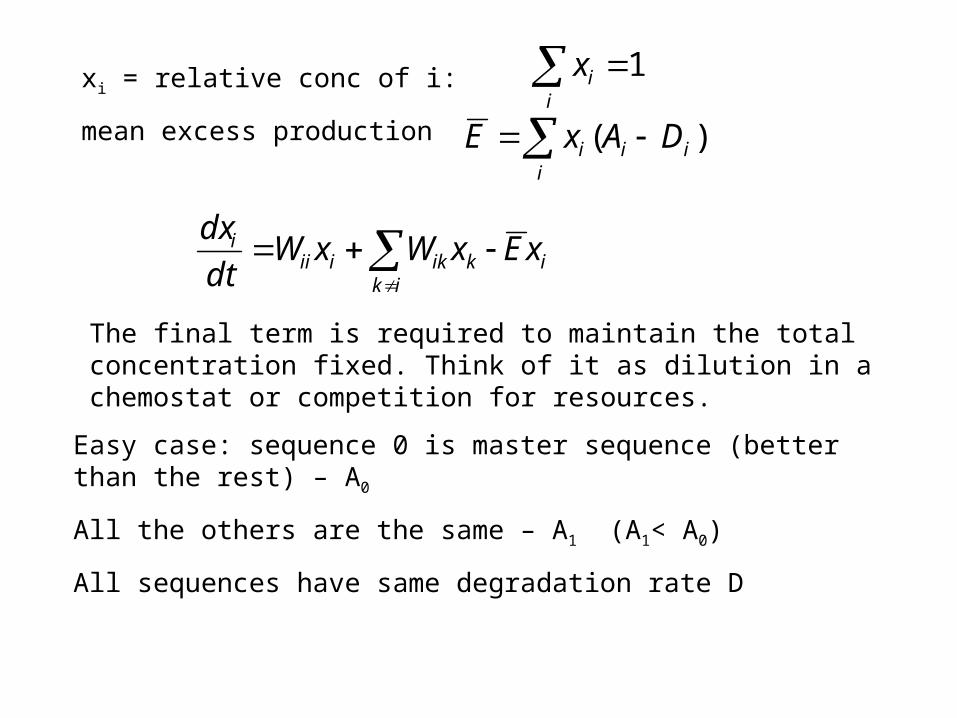
xi = relative conc of i:

mean excess production

i

ix 1

i

iii DAxE )(

iik

kikiiii xExWxWdt

dx

The final term is required to maintain the total concentration fixed. Think of it as dilution in a chemostat or competition for resources.

Easy case: sequence 0 is master sequence (better than the rest) – A0

All the others are the same – A1 (A1< A0)

All sequences have same degradation rate D

DqAW

DAAxADAxDAxEL

000

10011000 )())(1()(

00

00000 xExWxWdt

dx

kkk

forget back mutation when L >> 1

Concentrations are at equilibrium when

i.e. when

00 dt

dx

EW 00

10

100 AA

AqAx

L

Error threshold occurs when x0 0

For master sequence to survive, must have

01 / AAqL

Example with L = 50, A0=10, A1=1

error threshold when

q50 = 0.1 q = 0.955

error rate u = 1-q = 0.045

Master seq only Quasispecies Random sequences

Implications of the error threshold #1

01 / AAqL

10 /)1( AAu L

01 /)1( AAu L

)/ln()1ln( 10 AAuL

if L >> 1 and u << 1, this becomes )/ln( 10 AALu

If L is fixed there is a maximum error rate at which the master sequence survives.

If u is fixed there is a maximum length that can survive

Max is of order 1 mutation per whole genome replication.

Eigen paradox – longer molecules will likely be better replicators, but longer molecules require better accuracy...

How could first replicators overcome this?

Implications of the error threshold #2

Viruses are present as quasispecies – mutations occur within a patient. Difficult to get effective drugs.

RNA viruses have high mutation rates – u = 10-4 - 10-6 per base

DNA viruses 10-7 – 10-8

DNA genomes in cells 10-9 – 10-10

Viruses limited in size by mutation rate

Maybe high rate is advantageous too...

Mutation rate inversely proportional to genome size

‘Bag of Genes’ model

Simulations by Gocmanac & Higgs. Based on Stochastic Corrector model of Szathmary & Demeter.

Cell requires K (=3) types of gene. Alive if it has at least 1 of each.

Lattice with one cell per site.

Pick a cell. Duplicate one gene in the cell at random. If cell reaches max size M, divide randomly. Put one cell in parent position and one on a neighbouring site (overgrowth/competition).

Simplest Case

• M=14• Inviable cells (white)• Viable cells (black)

Fraction of viable cells increases with M.

Whole population dies if M too small.

Parasites / Selfish genes• A parasite occasionally arises by mutation• Parasites (pink) replicate faster within the cell• Don’t contribute to cell survival• Increase likelihood of creating inviable cells

Parasites created at low rate

Black = no parasites; Brown = At least one parasite

Pink = more than half the genes are parasites

M = 14 M = 40

clusters of infected cells are related

Fraction of viable cells as a function of M

If M is heritable, cells evolve to an optimal division size

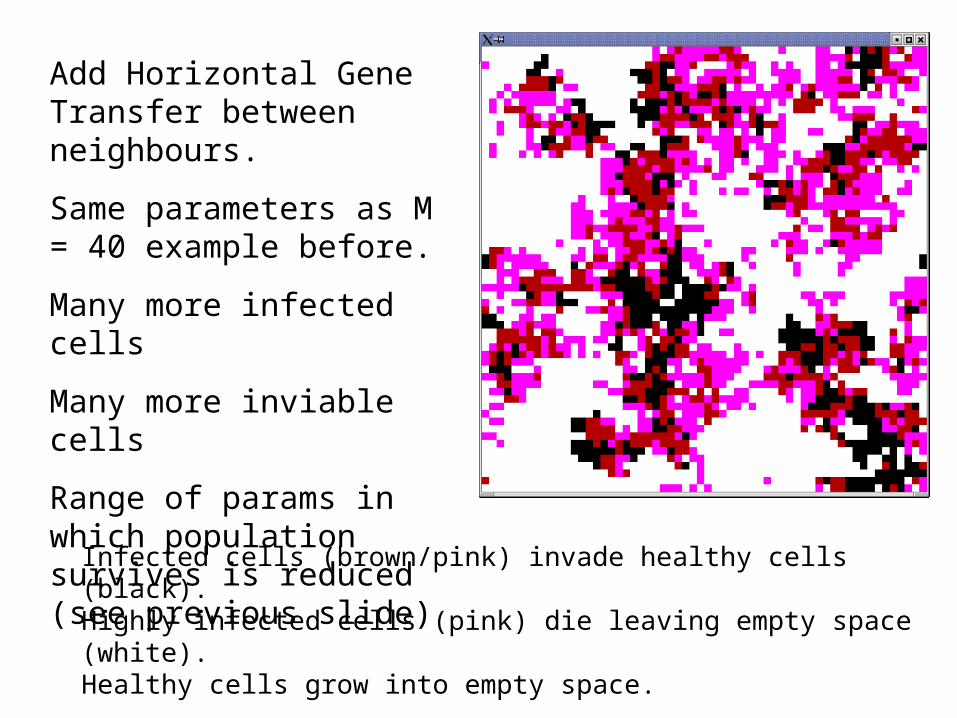
Add Horizontal Gene Transfer between neighbours.

Same parameters as M = 40 example before.

Many more infected cells

Many more inviable cells

Range of params in which population survives is reduced (see previous slide)

Infected cells (brown/pink) invade healthy cells (black).Highly infected cells (pink) die leaving empty space (white).Healthy cells grow into empty space.

Significance of horizontal gene transfer

Phylogenetic trees derived from different genes not always the same

Different strains of same bacterial species differ in gene content (e.g E. coli)

HGT may have been more frequent in the past. Maybe there is no tree? (Doolittle)

Alternative view – there is a core of genes that follows the organismal tree and there is some HGT superimposed on this.

If HGT was very frequent in early evolution, there would be no separate species. Communally evolving network of cells (Woese).

HGT aids the spread of new beneficial genes but it also makes parasites much more serious. Which is most important?

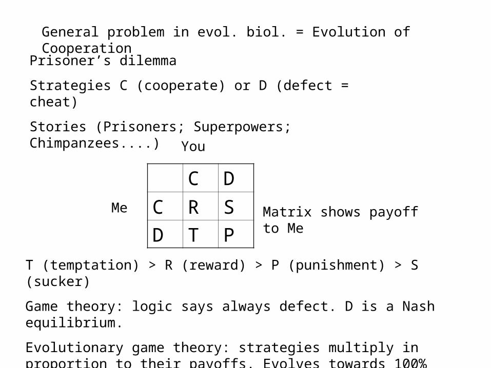
General problem in evol. biol. = Evolution of Cooperation

Prisoner’s dilemma

Strategies C (cooperate) or D (defect = cheat)

Stories (Prisoners; Superpowers; Chimpanzees....)

C D

C R S

D T P

You

Me Matrix shows payoff to Me

T (temptation) > R (reward) > P (punishment) > S (sucker)

Game theory: logic says always defect. D is a Nash equilibrium.

Evolutionary game theory: strategies multiply in proportion to their payoffs. Evolves towards 100% defectors. D is an Evolutionarily Stable Strategy (ESS).

Spatial Prisoners Dilemma (Nowak & May, 1992)

Each individual plays against its 8 lattice neighbours and a copy of itself.

Get score for each individual. At next timestep, each site is occupied by a copy of the best-scoring site in its neighbourhood.

Blue – is C, was C; Green – is C, was D;Red – is D, was D; Yellow – is D, was C.

Clusters of Cs survive. Hooray!

Cs have relatives on neighbouring sites.

Cs would die out if randomly mixed.

Q experiments (Spiegelmann)

Q is a bacteriophage – virus RNA length ~ 4000

Codes for a replicase protein.

Works in vitro.

add virus RNA

allow to replicate, then transfer small amount to next tube

analyse sequences in last tube

Sequences evolve towards short lengths (~200).

These are rapidly replicated but cannot function as viruses. Function is lost because it is not necessary.

“Spiegelmann’s monster”.

Cooperation between replicators – Szabo et al. (2002)

ADDBCAAAAAAAACBBCCCABBBBBBBBBBBBBBBBADADDDDAADCCCCCCCDDDDDDADB

nA nB nC

Sequences of four letters: A B C D

A controls template efficiency t(nA)

B controls replicase efficiency r(nB)

C controls replicase fidelity f(nC)

D is dummy nA

t(nA)

Each site on lattice is empty or contains one sequence.

Pick a site at random. The sequence on this site decays with a certain prob, or it is replicated by a neighbour with a certain prob.

replication rate ~ rt/n (t = template efficiency of the sequence being copied; r = replicase eficiency of the neighbour; n = total length of the sequence being copied).

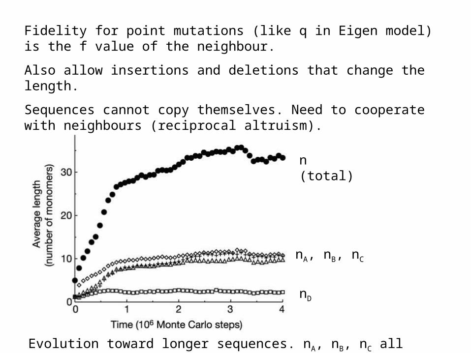
n (total)

nA, nB, nC

nD

Evolution toward longer sequences. nA, nB, nC all selected but not nD

Fidelity for point mutations (like q in Eigen model) is the f value of the neighbour.

Also allow insertions and deletions that change the length.

Sequences cannot copy themselves. Need to cooperate with neighbours (reciprocal altruism).

Length distribution is bimodal.

Long sequences are cooperators. They have good fidelity, replicase and template ability.

Short sequences are defectors – selfish genes –

They mostly have template ability only – like the Q monsters.

The spatial arrangement is important.

Sequences replicate neighbours. There are clusters of cooperators.

If you allow mixing (diffusion on lattice) then defectors win. Total length goes down. Efficient replicators cannot evolve.

Begin with previous case. Then turn on diffusion.

n goes down.

We have seen two ways in which replicators might cooperate and avoid being overrun by selfish genes.

1. Compartments – as in stochastic corrector mechanism. Cells contain groups of moderate numbers of sequences. Random segregation creates variation between cells. Evolution selects those with fewer parasites.

2. Spatial distribution – as in lattice models. Clusters of cooperators can survive even if they would not survive in a freely mixed system.

Autocatalytic sets

f1, f2 ... are food molecules supplied from outside

a, b, c ... are other molecules made by metabolism

White circles are reactions. Dashed arrows indicate catalysis

Reflectively autocatalytic – each molecule can be built from other molecules in the set and the food molecules; each formation reaction is catalyzed by other molecules in the set.

Constructively autocatalytic – the set can be built up sequentially via catalyzed reactions starting from the food set.

definitions from Mossel and Steel (2005) J. Theor. Biol.

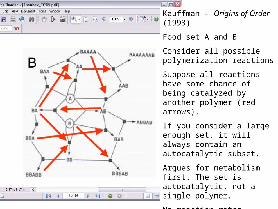
Kauffman – Origins of Order (1993)

Food set A and B

Consider all possible polymerization reactions

Suppose all reactions have some chance of being catalyzed by another polymer (red arrows).

If you consider a large enough set, it will always contain an autocatalytic subset.

Argues for metabolism first. The set is autocatalytic, not a single polymer.

No reaction rates, concentrations or thermodynamics

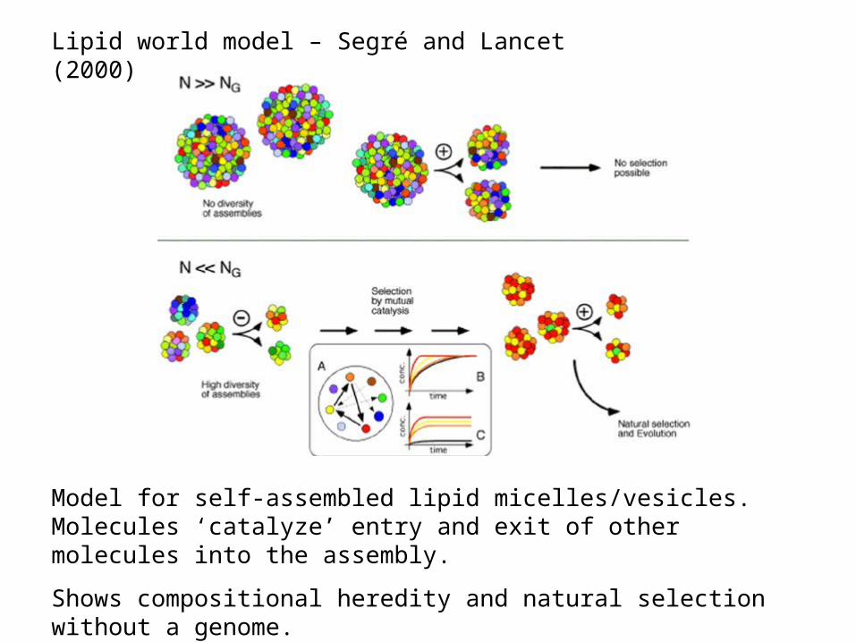
Lipid world model – Segré and Lancet (2000)

Model for self-assembled lipid micelles/vesicles. Molecules ‘catalyze’ entry and exit of other molecules into the assembly.

Shows compositional heredity and natural selection without a genome.