Escaping the Great Recession1 - Becker Friedman Institute · The shock follows a two-state Markov-switching process with transition matrix Hd The representative –rm faces... 1

Introduction The Model Estimation Trade-O¤ and Resolution Conclusions

Escaping the Great Recession1

Francesco Bianchi Leonardo MelosiCornell and Duke FRB ChicagoCEPR and NBER

Next Steps for the Fiscal Theory of the Price LevelBecker Friedman Institute

1The views in this paper are solely the responsibility of the authors andshould not be interpreted as re�ecting the views of the Federal Reserve Bank ofChicago or any other person associated with the Federal Reserve System.


The Great Recession and Policy InterventionsThe recent recession has induced:

1. Signi�cant changes in the conduct of monetary policy, withinterest rates stuck at the zero lower bound

� Standard new-Keynesian model would predict de�ation (BobHall�s puzzle)

2. A debate on the best way to mitigate the consequences of arecession when at the zero-lower-bound:

� Robust �scal intervention combined with a reduction in thefocus on in�ation

� Reluctance to explicitly abandon macroeconomic policies thathave been successful in the past


Model SetupWe model an economy in which:

1. recurrent large negative demand shocks can force theeconomy to the zero lower bound

2. two policy combinations characterize policy makers�behavior:

� Monetary led policy mix: The �scal authority strongly reacts todebt and the monetary policy rule satis�es the Taylor principle

� Fiscally led policy mix: The �scal authority disregards the levelof debt and the Taylor principle does not hold

Agents are aware of the possibility of...

1. ...zero lower bound episodes,

2. ...changes in policy makers�behavior,

3. ...and the link between the two


Main Results

1. The model accounts for the absence of de�ation during theGreat Recession as a result of policy uncertainty about howthe rising stock of public debt will be stabilized

2. At the zero lower bound a policy trade-o¤ arises...

� Announcing that �scal discipline will be abandoned greatlymitigates the recession, but...

� ...it also jeopardizes long-run macroeconomic stability

3. Policymakers could escape the Great Recession by committingto in�ating away only the amount of debt that results fromthe recession itself


Private sector

The representative household...

1. ...maximizes expected utility

2. ...is subject to a discrete preference shock d ξdt(high or low).

The shock follows a two-state Markov-switching process with

transition matrix Hd

The representative �rm faces...

1. ...a downward sloping demand curve

2. ...price stickiness


Government: Monetary/�scal policy mixMonetary rule (linearized):

eRt =h1� Zξdt

i " (1� ρR )�

ψπ,ξpteπt + ψy ,ξpt [byt � by �t ]�+

ρR ,ξpteRt�1 + σR εR ,t

#+Zξdt

[Zero Lower Bound]

Fiscal rule:

eτt = ρτ,ξpteτt�1+�1� ρτ,ξpt

� hδb,ξpt

ebmt�1 + ...i+στετ,t , ετ,t � N (0, 1)

Government budget constraint + (simpli�ed) �scal rule:

ebmt = β�1ebmt�1 + bmβ�1�bRmt�1,t � eπt � growth�

�eτt + spending! ebmt = �β�1 � δb,ξpt

� ebmt�1 + ...


In and out of the zero lower bound1. Out of the zero lower bound, two alternative policy regimes:

� Monetary led policy mix (AM/PF , Zξdt= 0):

ψπ

�ξpt = M; ξdt = h

�= ψπ,M > 1

δb

�ξpt = M; ξdt = h

�= δb,M > β�1 � 1

� Fiscally led policy mix (PM/AF , Zξdt= 0):

ψπ

�ξpt = F ; ξdt = h

�= ψπ,F < 1

δb

�ξpt = F ; ξdt = h

�= δb,F < β�1 � 1

2. Negative preference shock ! Zero lower bound policy mix :

Zξdt= 1! Rt ! ψzR

�1

δb

�ξpt = Z ; ξdt = l

�= δb,Z = 0


Evolution of Policy Regimes In and Out the ZLB

� Out of the zero lower bound, policymakers�behavior evolvesaccording to

Hp =�

pMM 1� pFF1� pMM pFF

�� Combine Hd with Hp to obtain evolution of policy regimes inand out the ZLB:

H =

24 phhHp (1� pll )�

pMZ1� pMZ

�(1� phh) [1, 1] pll

35


Estimation

� We solve the model with the method proposed by Farmer,Waggoner, and Zha (2009):

St = C (ξt , θ,H) + T (ξt , θ,H) St�1 + R (ξt , θ,H) εt

� Agents take into account the possibility of regime changes )Their beliefs matter for the solution of the model.

� We estimate the model with Bayesian methods over theperiod 1954:Q4-2014:Q1.

� Regime sequence based on MS-VAR evidence ( details ) andconsistent with Bianchi and Ilut (2016):

1. 1960s - 1970s ! Fiscally led policy mix2. 1980s - 2000s ! Monetary led policy mix3. Post-2008:Q4 ! Zero lower bound policy mix


Prior and Posterior Moments

Mean 5% 95% Type Mean Std

ψπ,M 1.6019 1.1758 2.0207 N 2.5 0.3ψy ,M 0.5065 0.2980 0.7688 G 0.4 0.2δb,M 0.0712 0.0457 0.1041 G 0.07 0.02ψπ,F 0.6356 0.5007 0.7546 G 0.8 0.3ψy ,F 0.2709 0.2005 0.3458 G 0.15 0.1δb,F 0 - - F 0 0d l �0.3662 �0.4827 �0.2789 N �0.3 0.1phh 0.9995 0.9984 0.9999 D 0.96 0.03pll 0.9306 0.8936 0.9599 D 0.83 0.10pMM 0.9923 0.9872 0.9965 D 0.96 0.03pFF 0.9923 0.9888 0.9951 D 0.96 0.03pMZ 0.9225 0.8108 0.9861 D 0.50 0.22


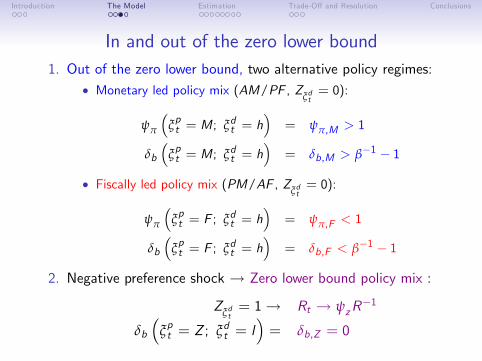
Dynamics at the ZLB

2007 2008 2009 2010 2011 2012 2013 2014

2

1

0

GDP growth

2007 2008 2009 2010 2011 2012 2013 2014

0.5

0

0.5

1

Inflation

2007 2008 2009 2010 2011 2012 2013 2014

0.20.40.60.8

11.2

FFR

Actual dataMedian90% Error Bands

2007 2008 2009 2010 2011 2012 2013 2014

150

200

250

300

DebttoGDP


No Policy Uncertainty

Let us consider a counterfactual that removes policy uncertainty:Only Monetary led regime out of the ZLB

2007 2008 2009 2010 2011 2012 2013 201420

15

10

5

0GDP growth

2007 2008 2009 2010 2011 2012 2013 201415

10

5

0

Inflation

2007 2008 2009 2010 2011 2012 2013 2014

200

400

600

800

1000

1200

1400

DebttoGDP

BenchmarkOnly Monetary led


In�ation Expectations

Corroborating evidence: In�ation expectations

2007 2008 2009 2010 2011 2012 2013 20140

0.5

1

1.5

Oneyear horizon

Michigan surveyMedian90% error bands

2007 2008 2009 2010 2011 2012 2013 20140

0.5

1

1.5

Fiveyear horizon


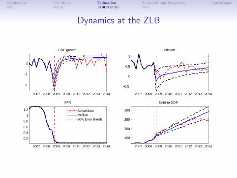
No �scal block: Explanatory power of discrete shock

Suppose we estimate a nested model without the �scal block:! It cannot account for the joint dynamics of growth and in�ationwith a single shock

2007 2008 2009 2010 2011 2012 2013 20142.5

2

1.5

1

0.5

0

0.5

GDP growth

2007 2008 2009 2010 2011 2012 2013 2014

0.5

0

0.5

1

Inflation

Benchmark ModelActual dataMedian90% Error Bands

Table


No �scal block: Ability to match in�ation expectations

Suppose we estimate a nested model without the �scal block:! It cannot account for the behavior of in�ation expectations

2007 2008 2009 2010 2011 2012 2013 20140

0.5

1

1.5

Oneyear horizon

2007 2008 2009 2010 2011 2012 2013 20140

0.5

1

1.5

Fiveyear horizon

Benchmark ModelMichigan surveyMedian90% error bands

Table


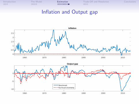
In�ation and Output gap

1960 1970 1980 1990 2000 2010

0

0.5

1

1.5

2

2.5

Inflation

1960 1970 1980 1990 2000 2010

10

5

0

Output gap

BenchmarkNo Fiscal Uncertainty


Policy Trade-O¤

Why do not policy makers simply announce a switch to the �scallyled regime?

� Announcing the Fiscally led regime...

1. ...mitigates the recession...2. ...at the cost of an increase in macroeconomic uncertainty

� The two results are the two sides of the same coin

� Announcement works only if it modi�es long termexpectations about future policy makers�behavior


Escaping the Great Recession

Suppose policy makers commit to in�ating away only the amountof debt resulting from the recession itself ) No large recession

10 20 30 40 50 60

10

5

0Output gap

10 20 30 40 50 60

0.5

0

0.5

1

Inflation

10 20 30 40 50 60

0.2

0.40.6

0.8

1

1.2

FFR

Escaping ruleBenchmark

10 20 30 40 50 60

150

200

250

300

350

400

DebttoGDP


Escaping the Great Recession

Policy makers follow the Monetary led policy mix in response to allother shocks ) No increase in uncertainty

10 20 30 40 50 60

1

1.2

1.4Output gap

One

qua

rter

10 20 30 40 50 600.35

0.40.45

0.50.55

Inflation

10 20 30 40 50 60

2

3

4

One

yea

r

10 20 30 40 50 600.4

0.6

0.8

10 20 30 40 50 602

4

6

Two

year

10 20 30 40 50 600.4

0.6

0.8

Escaping ruleBenchmark


Concluding Remarks

1. Recurrent ZLB events in a standard DSGE model

2. Absence of de�ation explained by policy uncertainty inresponse to a single shock

3. The model highlights a policy trade o¤ that can explain whypolicy makers...

� are reluctant to abandon �scal discipline

� might be tempted to do so to escape the Great Recession

4. In�ating away only the amount of debt accumulated becauseof the recession would resolve the trade o¤


EXTRAS


Motivating evidence Back

� We use a MS-VAR to establish a series of stylized facts:

Zt = cξΦt+ AξΦ

t ,1Zt�1 + AξΦ

t ,2Zt�2 + Σ1/2

ξΣt

ωt

ΦξΦt=

hcξΦ

t,AξΦ

t ,1,AξΦ

t ,2

i, ωt � N(0, I )

� The model allows for three regimes for the VAR coe¢ cientsand three regimes for the covariance matrix

� We include four observables:1. Primary de�cit-to-GDP ratio2. GDP growth3. In�ation4. Federal Funds Rate


Regime probabilities Back


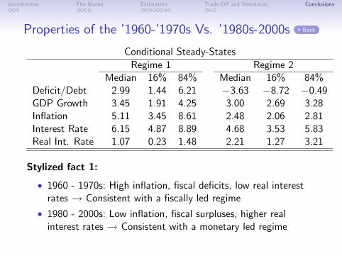
Properties of the �1960-�1970s Vs. �1980s-2000s Back

Conditional Steady-StatesRegime 1 Regime 2

Median 16% 84% Median 16% 84%De�cit/Debt 2.99 1.44 6.21 �3.63 �8.72 �0.49GDP Growth 3.45 1.91 4.25 3.00 2.69 3.28In�ation 5.11 3.45 8.61 2.48 2.06 2.81Interest Rate 6.15 4.87 8.89 4.68 3.53 5.83Real Int. Rate 1.07 0.23 1.48 2.21 1.27 3.21

Stylized fact 1:

� 1960 - 1970s: High in�ation, �scal de�cits, low real interestrates ! Consistent with a �scally led regime

� 1980 - 2000s: Low in�ation, �scal surpluses, higher realinterest rates ! Consistent with a monetary led regime


Properties of the zero lower bound regime Back

2009 2010 2011 2012 2013 2014

0

5

10

15

20Deficit/Debt

2009 2010 2011 2012 2013 20144

2

0

2

4GDP Growth

2009 2010 2011 2012 2013 20140

0.5

1

1.5

2

Inflation

2009 2010 2011 2012 2013 20140.5

0

0.5

1

1.5

FFR

70% BandsDiscrete ShocksData

Stylized fact 2: One single event is able to account for the zerolower bound dynamics


Fiscal shocks Back

0 10 2042024

2008

:Q3

0 10 20

0

1

2

Pos

t20

08:Q

3

0 10 20

1012

Pre

200

8:Q

3 Deficit/Debt

0 10 20

0123

0 10 20

0

0.5

1

0 10 200

0.5

1GDP growth

0 10 20

0

0.5

1

0 10 20

0.2

0

0.2

0 10 200.2

0

0.2Inflation

0 10 201.5

10.5

0

0 10 20

0.1

0

0.1

0 10 200

0.5

1FFR

Stylized fact 3: Fiscal imbalances are important at the zero lowerbound


Desirable properties

Desirable properties of a model aiming to explain the zero lowerbound dynamics:

1. A single large initial shock should account for the dynamics ofmacro aggregates

2. The model should distinguish three periods in US economichistory

3. The model should capture the in�ationary consequences of�scal imbalances during the zero lower bound

Back


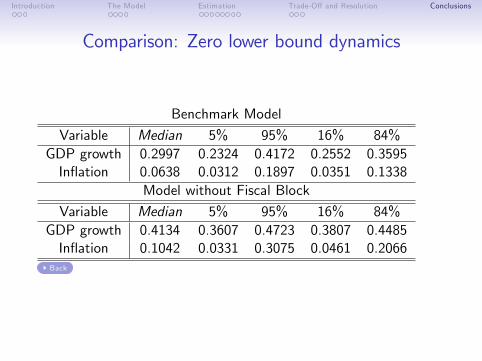
Comparison: Zero lower bound dynamics

Benchmark Model

Variable Median 5% 95% 16% 84%GDP growth 0.2997 0.2324 0.4172 0.2552 0.3595In�ation 0.0638 0.0312 0.1897 0.0351 0.1338

Model without Fiscal Block

Variable Median 5% 95% 16% 84%GDP growth 0.4134 0.3607 0.4723 0.3807 0.4485In�ation 0.1042 0.0331 0.3075 0.0461 0.2066

Back


Comparison: Ability to match in�ation expectationsBenchmark Model

Variable Median 5% 95% 16% 84%Whole sample: 1-year 0.0569 0.0374 0.0857 0.0440 0.0733Whole sample: 5-year 0.0451 0.0345 0.0641 0.0378 0.0557Pre-ZLB: 1-year 0.0424 0.0317 0.0615 0.0349 0.0529Pre-ZLB: 5-year 0.0493 0.0383 0.0734 0.0415 0.0625Post-ZLB: 1-year 0.1001 0.0368 0.2067 0.0551 0.1595Post-ZLB: 5-year 0.0181 0.0037 0.0958 0.0066 0.0532

Model without Fiscal Block

Variable Median 5% 95% 16% 84%Whole sample: 1-year 0.1675 0.1399 0.1955 0.1510 0.1840Whole sample: 5-year 0.1563 0.1106 0.2141 0.1307 0.1894Pre-ZLB: 1-year 0.1496 0.1241 0.1880 0.1349 0.1696Pre-ZLB: 5-year 0.1836 0.1281 0.2557 0.1510 0.2229Post-ZLB: 1-year 0.2309 0.1005 0.3008 0.1577 0.2778Post-ZLB: 5-year 0.0656 0.0139 0.1369 0.0298 0.1058

Back


Dynamics at the ZLB

� Impulse response to a discrete negative preference shock d l

� We consider the economy as it was in 2008Q3

� A negative discrete preference shock occurs in 2008:Q4

� Objectives:

1. A stylized NK model can replicate the key post-2008Q3macroeconomic facts as a result of only one shock

2. The impulse response is not invariant with respect to the stateof the economy; in particular the �scal situation

� b/c the negative preference shock implies a change inexpectations about future policymakers�behavior


Primary de�cit and debt� The government budget constraint is given by:

bmt =�bmt�1R

mt�1,t

�/ (ΠtYt/Yt�1) + pdt

where bmt = (Pmt B

mt ) / (PtYt ) and all variables are expressed

as a faction of GDP� In steady state:

bm = (bmRm) / (ΠM) + pd

bm =pd

1� (1+ r) / (1+ γ)

bm =pd

1� 1/β> 0 if pd < 0

� Also:pdbm

= 1� 1/β < 0


Shock to government spending

5 10 15 200

0.01

0.02

0.03

0.04

0.05

0.06

Inflation

5 10 15 20

0

0.05

0.1

0.15

0.2

0.25

0.3

Output gap

5 10 15 200

0.01

0.02

0.03

0.04

0.05

FFR

Monetary ledFiscally ledZLB


Monetary/Fiscal Policy Mix

Leeper (1991) shows that two determinacy regions exist:

ψπ,ξptδb,ξpt

Active Monetary, Passive Fiscal > 1 > β�1 � 1Passive Monetary, Active Fiscal < 1 < β�1 � 1

� AM/PF ! Taylor principle is satis�ed, �scal policyaccommodates behavior of monetary authority! Macroeconomy is insulated (Ricardian regime)

� PM/AF ! Taylor principle is not satis�ed, in�ation is free tomove to keep debt on a stable path! Macroeconomy is not insulated (non-Ricardian regime)


Why does this approach work?

� Policy makers are in�uencing agents�beliefs about their longrun behavior in response to a speci�c shock

� Automatic stabilizer: This behavior determines an increase inshort run expected in�ation exactly when necessary

� Policy makers are committed to raise taxes to repay thepreexisting amount of debt and all future �scal imbalances

� Macroeconomic stability is retained after the recession

Documents

Escaping the Great Recession1 - Becker Friedman Institute · The shock follows a two-state Markov-switching process with transition matrix Hd The representative –rm faces... 1