Essays in Applied Microeconomics - Harvard University

Essays in Applied MicroeconomicsThe Harvard community has made this

article openly available. Please share howthis access benefits you. Your story matters

Citation Spamann, Holger. 2012. Essays in Applied Microeconomics. Doctoraldissertation, Harvard University.

Citable link http://nrs.harvard.edu/urn-3:HUL.InstRepos:9393267

Terms of Use This article was downloaded from Harvard University’s DASHrepository, and is made available under the terms and conditionsapplicable to Other Posted Material, as set forth at http://nrs.harvard.edu/urn-3:HUL.InstRepos:dash.current.terms-of-use#LAA

http://osc.hul.harvard.edu/dash/open-access-feedback?handle=&title=Essays%20in%20Applied%20Microeconomics&community=1/1&collection=1/4927603&owningCollection1/4927603&harvardAuthors=384eb52424f55954e9a57dad134e6887&departmentEconomics

http://nrs.harvard.edu/urn-3:HUL.InstRepos:9393267

http://nrs.harvard.edu/urn-3:HUL.InstRepos:dash.current.terms-of-use#LAA



c©2012 – Holger Spamann

All rights reserved.

Thesis advisor Author

Professor Andrei Shleifer Holger Spamann

Essays in Applied Microeconomics

Abstract

Chapter 1 develops a model of parallel trading of corporate securities (shares, bonds)

and derivatives in which a large trader can sometimes profitably acquire securities and the

corporate control rights inherent therein for the sole purpose of reducing the corporation’s

value and gaining on a net short position in the corporation created through off-setting

derivatives. At other times, the large trader profitably takes a net long position in the cor-

poration and exercises its control rights to maximize the corporation’s value. This strategy

is profitable if and because other market participants cannot observe the large trader’s or-

ders and hence cannot predict how the control rights will be exercised. In effect, the large

trader is benefitting from trading on private information about payoff uncertainty that the

large trader itself creates. This problem is most likely to manifest in transactions that

give blocking powers to small minorities, particularly out-of-bankruptcy restructurings and

freezeouts, and is bound to become more severe when derivatives trade on an exchange

rather than over-the- counter.

Chapter 2 investigates in parallel the cross-country determinants of crime and punish-

ment in the largest possible sample of countries with data on homicides, victimization by

iii

Abstract iv

common crimes (ICVS), incarceration rates, and the death penalty. While models with

a small number of plausible covariates predict much of the variation of homicide and in-

carceration rates between major developed countries, they predict only one seventh of the

actual US incarceration rate.

Chapter 3 probes into the pervasive correlations between legal origins, modern regu-

lation, and economic outcomes around the world. Where legal origin is exogenous, it is

almost perfectly correlated with another set of potentially relevant background variables:

the colonial policies of the European powers that spread the "origin" legal systems through

the world. The chapter attempts to disentangle these factors by exploiting the imperfect

overlap of colonizer and legal origin, and looking at possible channels, such as the structure

of the legal system, through which these factors might influence contemporary economic

outcomes. It find strong evidence in favor of non-legal colonial explanations for economic

growth. For other dependent variables, the results are mixed.

Contents

Title Page . . . . . . . . . . . . . . . . . . . . . . . . . . . . . . . . . . . . . . iAbstract . . . . . . . . . . . . . . . . . . . . . . . . . . . . . . . . . . . . . . . iii

1 Derivatives Trading and Negative Voting 11.1 Introduction . . . . . . . . . . . . . . . . . . . . . . . . . . . . . . . . . . 11.2 The Economic Mechanism . . . . . . . . . . . . . . . . . . . . . . . . . . 41.3 The Formal Model . . . . . . . . . . . . . . . . . . . . . . . . . . . . . . 7

1.3.1 Model Setup . . . . . . . . . . . . . . . . . . . . . . . . . . . . . 71.3.2 Equilibrium Concept . . . . . . . . . . . . . . . . . . . . . . . . . 121.3.3 Equilibrium in the General Case . . . . . . . . . . . . . . . . . . . 131.3.4 Equilibrium with quadratic cost, uniform voting threshold distribu-

tion, and symmetric liquidity trades . . . . . . . . . . . . . . . . . 171.3.5 Multiple Hedge Funds . . . . . . . . . . . . . . . . . . . . . . . . 18

1.4 Discussion . . . . . . . . . . . . . . . . . . . . . . . . . . . . . . . . . . . 191.4.1 Derivatives vs. other hedges . . . . . . . . . . . . . . . . . . . . . 191.4.2 Required control stakes . . . . . . . . . . . . . . . . . . . . . . . . 201.4.3 Legal constraints . . . . . . . . . . . . . . . . . . . . . . . . . . . 21

1.5 Conclusion . . . . . . . . . . . . . . . . . . . . . . . . . . . . . . . . . . 22

2 American Exceptionalism Revisited: The Global Cross-Section of Crime andPunishment 232.1 Introduction . . . . . . . . . . . . . . . . . . . . . . . . . . . . . . . . . . 232.2 Structural vs. reduced form equations . . . . . . . . . . . . . . . . . . . . 27

2.2.1 A simple model of the simultaneity problem . . . . . . . . . . . . . 272.2.2 The absence of valid instruments . . . . . . . . . . . . . . . . . . . 282.2.3 Reduced-form equations . . . . . . . . . . . . . . . . . . . . . . . 29

2.3 Dependent Variables . . . . . . . . . . . . . . . . . . . . . . . . . . . . . 302.3.1 Crime . . . . . . . . . . . . . . . . . . . . . . . . . . . . . . . . . 302.3.2 Punishment . . . . . . . . . . . . . . . . . . . . . . . . . . . . . . 32

2.4 Independent variables . . . . . . . . . . . . . . . . . . . . . . . . . . . . . 332.5 Regression specifications . . . . . . . . . . . . . . . . . . . . . . . . . . . 41

2.5.1 General issues . . . . . . . . . . . . . . . . . . . . . . . . . . . . 41

v

Contents vi

2.5.2 ICVS data . . . . . . . . . . . . . . . . . . . . . . . . . . . . . . . 432.6 Basic results and discussion . . . . . . . . . . . . . . . . . . . . . . . . . . 44

2.6.1 Variables associated with differences in crime and punishment . . . 502.6.2 Variables associated with differences in crime . . . . . . . . . . . . 512.6.3 Variables associated with differences in punishment . . . . . . . . . 522.6.4 Variables not robustly associated with either crime or punishment . 52

2.7 Robustness . . . . . . . . . . . . . . . . . . . . . . . . . . . . . . . . . . 542.7.1 Developed countries only (EU & OECD) . . . . . . . . . . . . . . 552.7.2 Prison populations in the 1970s . . . . . . . . . . . . . . . . . . . 562.7.3 Drug-related deaths . . . . . . . . . . . . . . . . . . . . . . . . . . 58

2.8 Discussion: Legal Origins . . . . . . . . . . . . . . . . . . . . . . . . . . 602.9 Conclusion . . . . . . . . . . . . . . . . . . . . . . . . . . . . . . . . . . 64

3 Legal Origin or Colonial History? 663.1 Introduction . . . . . . . . . . . . . . . . . . . . . . . . . . . . . . . . . . 663.2 Empirical Strategy - Independent Variables . . . . . . . . . . . . . . . . . 72

3.2.1 Countries for which legal origin and colonial history do not coincide 723.2.2 Institutional channels . . . . . . . . . . . . . . . . . . . . . . . . . 78

3.3 Growth . . . . . . . . . . . . . . . . . . . . . . . . . . . . . . . . . . . . 823.4 Other Dependent Variables: Financial Markets, Unemployment, and Insti-

tutions . . . . . . . . . . . . . . . . . . . . . . . . . . . . . . . . . . . . . 953.5 Discussion . . . . . . . . . . . . . . . . . . . . . . . . . . . . . . . . . . . 1003.6 Conclusion . . . . . . . . . . . . . . . . . . . . . . . . . . . . . . . . . . 101

References 102

Chapter 1

Derivatives Trading and Negative Voting

1.1 Introduction

Securities regulators, practitioners, and legal commentators worry that derivatives may

provide shareholders and creditors incentives to destroy value in their corporation.1 The ba-

sic concern is that if shareholders or creditors own a sufficient amount of off-setting deriva-

tives such as put options or credit default swaps (CDS), any losses on their shares or debt

will be more than off-set by the corresponding gains on their derivatives ("over-hedging").

In this case, shareholders and creditors benefit by using the control rights inherent in their

shares or debt to reduce the corporation’s value ("negative voting"). An important question

that is generally not considered, however, is whether it would ever be profitable for share-

holders or creditors to acquire so many derivatives in the first place. After all, any gains to

shareholders and creditors come at the expense of their counterparties on their derivative

contracts. These counterparties would therefore prefer not to sell the derivatives, or only

at a price that compensates them for the future payouts, thus depriving shareholders and

creditors of any profit in the overall scheme.

This paper argues that over-hedging and negative voting can indeed be profitable with

1Regulators: See, e.g., Securities and Exchange Commission, Concept Release on the U.S. Proxy System,75 Fed. Reg. 42,982, 43,017-20 (July 22, 2010); Committe of European Securities Regulators, PublicStatement of the Market Participants Consultative Panel CESR/10/567 (July 5, 2010), at 3-4. Practitioners:See, e.g., Soros (2010) and Sender (2009) (quoting from David Einhorn’s letter to investors). Commentators:See in particular Martin and Partnoy (2005) and Hu and Black (2007, 2008).

1

Chapter 1: Derivatives Trading and Negative Voting 2

a minimal and realistic degree of investor heterogeneity and asymmetric information. The

paper presents a model of parallel trading of corporate securities (shares, bonds) and deriva-

tives in which a large, strategic trader interacts with liquidity traders and competitive mar-

ket makers. The key assumptions are that market makers cannot observe the large trader’s

orders directly, and cannot infer them from aggregate order flow because of fluctuating liq-

uidity trades. In this case, market makers cannot predict how control rights will be exercised

if the large trader only over-hedges some of the time. Prices will reflect some probability

of negative voting, allowing the large trader to benefit from its private information about its

own trades and expected vote. In effect, the large trader is exploiting private information

about payoff uncertainty that the large trader itself creates. The large trader benefits at the

expense of liquidity traders, whose trades provide camouflage to the large trader.

The assumption that counterparties cannot observe the large trader’s positions and

hence its incentives for exercising control rights seems to capture many situations in real

world derivative markets. This is obvious to the extent derivatives are traded on an ex-

change and centrally cleared. Such anonymous trading has long been the standard for eq-

uity options and is now generally mandated by the Dodd-Frank Act. But even when trading

occurs over-the-counter (OTC), traders’ positions and strategies are confidential and remain

largely hidden from their counterparties (e.g., Avellaneda and Cont 2010 for the CDS mar-

ket). To be sure, any market participant in an OTC market knows the identity of it direct

counterparty, at least post-trade. But since dealers routinely enter into chains of hedging

transactions (e.g., Stulz 2010), the ultimate buyer of protection will usually be unaware of

the identity of the ultimate seller, and vice versa.2 In addition, investors can conceal their

overall position even from their direct counterparties by splitting trades among many of

them.

The foregoing assumption distinguishes the present paper from Bolton and Oehmke

(2011) and Campello and Matta (2012). These very insightful papers analyze the effect of

CDS availability on renegotiation in an incomplete contracting model of debt with strategic

default. In their model, creditors’ ability to hedge their exposure to the debtor with CDS

2Chen et al. (2011) report that dealers often do not hedge large trades right away but only in the courseof several days. Unless default of the reference entity is imminent, however, this does not change the basicpoint here.


contracts increases creditors’ bargaining power in renegotiation. This reduces the incidence

of strategic default and therefore has the beneficial effect of increasing the debt capacity

of the firm; at the same time, overinsurance may lead to an inefficiently high frequency

of bankruptcy. Crucially, these papers assume that the CDS protection sellers observe the

exact position of the buyer-creditor, who therefore never gains from dealing in CDS as

such. While this assumption is justified in many situations, the asymmetric information

scenario considered in the present paper seems better suited to other situations, particularly

for exchange trading of derivatives. In effect, a parallel reading of the aforementioned

papers and the present one demonstrates the crucial importance of CDS market structure

for discussing the costs and benefits of these derivatives.

The idea that a large trader can create uncertainty about the security payoff and profit on

a net long or a net short position is also present in Brav and Mathews (2011). In their model,

however, the only traded assets are shares, and the only way to create a short position is by

shorting the shares. To retain voting power while being short the shares, i.e., to over-hedge,

the hedge fund acquires naked votes from other shareholders through the share lending

market. Brav and Mathews assume that the hedge fund can do so for free up to a certain

amount, and not at all beyond that amount.3 This assumption does not work outside the

share lending market, however, because the hedge fund will have to pay for votes bundled

with a cash-flow into a security. Moreover, trading in derivatives presents additional profit

opportunities for the hedge fund.

The model closest to the present paper is parallel work by Zachariadis and Olaru (2011).

Theirs is a model of parallel trading of debt and equity, in which a hedge fund may build a

long position in a firm’s debt only to reject a restructuring and profit from a short position in

the firm’s equity. The main differences to the present paper are twofold. First, Zachariadis

and Olaru add another strategic player, namely the firm manager who makes a take-it-

or-leave-it restructuring offer to debtholders. Second, they consider only binary trading

choices in debt and equity, i.e., the hedge fund can only choose whether to trade, but not

how much. Qualitatively, they reach results similar to the present paper.

3Cf. Christoffersen et al. (2007), who document that the average vote does indeed sell for a price of zeroin the share lending market.


Empirical work on negative voting has been severely limited by the lack of investor-

level position and voting data. Papers that have looked at correlations between the avail-

ability of CDS and corporate bankruptcy have found mixed results, depending on the time

period studied and the construction of the sample (Peristiani and Savino 2011; Bedendo et

al. 2012). In the future, regulators may gain access to the requisite data for more probative

empirical studies. In the meantime, gaining a firm theoretical understanding of the question

remains of pressing importance.

1.2 The Economic Mechanism

To facilitate understanding of the formal model presented in the next section, this sec-

tion will lead with a verbal description of the main economic mechanism at work.

Imagine that two assets trade in a market with three types of participants. The traded

assets are bonds (publicly traded debt claims) and credit insurance on those bonds. The

market participants are a hedge fund, numerous benign traders such as pension funds and

mutual funds, and numerous competitive financial institutions that act as market makers.

The benign traders buy and sell random quantities regardless of price for exogenous pur-

poses such as fulfilling redemptions or purchases, portfolio rebalancing, or compliance with

fund risk policies. Competition between market makers ensures that the benign traders al-

ways obtain prices equal to the value that is expected given publicly available information.

The precise structure of trading will be discussed later.

After trading, the value of the bonds – and hence the payouts on credit insurance con-

tracts – will be determined by a bondholder vote on a proposed restructuring. For illustra-

tive purposes, assume that the bonds will be worthless if creditors reject the restructuring,

but pay the full face amount if creditors accept the restructuring. Conversely, credit insur-

ance will pay out nothing if the restructuring succeeds, and will pay the full insured amount

if the restructuring fails. Naturally, bondholders will accept the restructuring unless they

own more than full credit insurance on their bonds, i.e., unless they are over-hedged.

To keep things simple, assume that only one market participant – the hedge fund – is

ruthless enough to consider over-hedging and negative voting. That is, only the hedge fund


would purchase more credit insurance than bonds and attempt to block the restructuring.

One can imagine that reputational or regulatory concerns prevent other market participants

from considering this strategy. The probability that the hedge fund would be able to block

the restructuring is increasing in the number of bonds that the hedge fund owns. The will-

ingness of the hedge fund to block the restructuring depends only on the hedge fund’s rela-

tive holdings of bonds and credit insurance: if the hedge fund owns more credit insurance,

the hedge fund will attempt to block the restructuring; otherwise, it will not.

These assumptions imply that the expected value of the bonds – and the expected pay-

outs on the credit insurance – depends entirely on how many bonds and how much credit

insurance the hedge fund ends up owning. The problem for market makers is that they do

not know the hedge fund’s trades and ultimate position, and hence cannot determine exactly

how much the bonds or credit insurance will be worth. The crucial but realistic assumption

is that market makers cannot observe the hedge fund’s trades. In particular, the hedge fund

can conceal its trades by placing orders through different brokers. Market makers are able

to observe aggregate market turnover – through information repositories, or exchange data

–, but these aggregate numbers compound the hedge fund’s trades with the random trades

of benign traders.

The best that market makers will be able to do is to form expectations of the hedge

fund’s positions based on the aggregate trading data. Before discussing this inference prob-

lem, however, it is instructive to consider what would happen if market makers’ expecta-

tions did not depend on trading volume. Consider two extreme cases. If market makers

believed that the hedge fund will block the restructuring, the bond price would be zero

(recall that competition between market makers will push prices to expected value), while

credit insurance would cost exactly the insured amount. In this case, the hedge fund could

make (unlimited) profits by buying (all the) bonds for free, selling (unlimited amounts of)

insurance, and not preventing the restructuring. At the other extreme, if market makers

believed that the hedge fund will not block the restructuring, the bond price would be equal

to its face amount, while credit insurance would be costless. In this case, the hedge fund

could make unlimited profits by buying unlimited amounts of credit insurance for free and

just enough bonds to block the restructuring.

To analyze how market makers are going to form beliefs about the hedge fund’s po-


sitions from aggregate market data, it is necessary to specify the trading process in more

detail. The model considers the simplest possible market with only one round of trading.

First, the hedge fund and liquidity traders submit their orders (buys and sells). Second,

market makers observe aggregate orders. Third, market makers fill all these orders at com-

petitive prices, i.e., prices that correspond to their best estimate of the probability that the

hedge fund will block the restructuring.

In this setup, market makers beliefs about the hedge fund’s position will be based on

their observation of aggregate orders in combination with their prior beliefs about the dis-

tribution of benign traders’ orders. In particular, when the demand for bonds or derivatives

is extremely high or low (this includes negative demand), market makers will assume with

high probability that this demand emanates mostly from the hedge fund if and because

benign traders never submit such large orders. For more moderate values, market makers

will not know if they result from relatively high demand by the hedge fund and relatively

low demand by the benign market participants, or vice versa. In this case, market makers

must assign probability estimates based on the relative likelihood of these two scenarios,

and prices will reflect weighted average values.

These average prices enable the hedge fund to profit from mixing both strategies. Some-

times the hedge fund profits by over-hedging and blocking the restructuring. At other times,

the hedge fund gains by not over-hedging and letting the restructuring proceed because it

can buy the bond at a price discount, and sell credit insurance at a price premium, that

reflect the possibility of the restructuring being blocked. To be sure, the hedge fund cannot

predict benign traders demand. If high (low) demand by the hedge fund coincides with high

(low) demand by benign traders, market makers can infer the hedge fund’s positions and

hence accurately predict bond and insurance payoffs. In this case, the hedge fund does not

make any profits. When high hedge fund demand coincides with low demand by benign

traders and vice versa, however, the hedge fund makes a trading profit. In effect, the hedge

fund is trading on private information on its own value-relevant strategy.

Where do the hedge fund’s profits come from? Competitive market makers always trade

for prices that are equal to expected value, given their information. Consequently, market

makers make zero profits or losses. The hedge fund’s profits come out of the pockets of the

benign traders. They tend to sell many derivative contracts when pay-outs on the contracts


will turn out to be high relative to the contracts’ price, and they tend to buy many contracts

when pay-outs will turn out to be low relative to the contracts’ price.

As a final note, the size of the hedge fund’s positions depends on trading costs such

as commissions, bid-ask spreads, or margin requirements, and the variability of benign

traders’ demand. The higher the variability of benign traders’ demand, the bigger the

stakes that the hedge fund can hope to buy without being discovered, and hence the larger

the trading profits that the hedge fund can make. The higher the trading costs, the more

conservatively the hedge fund will trade. In the extreme, trading costs can be so high as to

make it impossible for the hedge fund to make any profits. In this sense, a more “liquid”

market facilitates over-hedging and negative voting.

1.3 The Formal Model

1.3.1 Model Setup

This subsection introduces the setup of the model: the two types of traded assets (secu-

rities and derivatives), the three types of market participants (hedge fund, liquidity traders,

and market makers), and trading including information. It concludes with some remarks

on this setup.

Timeline

The timeline of actions is as follows (details to follow in subsequent subsections):

1. The hedge fund and liquidity traders submit their orders.

2. The market makers observe only net market demand, which combines the hedge

fund’s and the liquidity traders’ orders. Based on this observation, market makers

update their beliefs about the expected value of the securities and derivatives. At

these values (prices), they fill all net orders.

3. Security holders choose between two actions by some voting mechanism.

4. Payoffs are realized.


Traded assets

There are two traded4 assets with perfectly negatively correlated payoffs: securities,

which will throughout be denoted by the letter X , and derivatives, which will throughout

be denoted by the letter Y . If the security pays v, the derivative pays 1− v. Consequently,

the derivative can be interpreted as an insurance claim on the security. In particular, if the

security were a bond, the derivative could be a credit default swap; if the security were a

share, the derivative could be a total equity return swap.

The number of securities is normalized to one (of which infinitesimal divisions are

traded). The derivative is a synthetic asset; hence its net supply is zero but unlimited

amounts can be sold and bought. Short-selling is allowed for both derivatives and securities.

The security payoff v depends on a binary choice between two actions, which is deter-

mined by a vote of the security holders. For example, if the security is a bond, the choice

could be whether or not to agree to a proposed restructuring; if the security is a share,

it could be whether or not to agree to a merger. Normalize the payoff when the "right"

decision is taken to v = 1, and when the "wrong" decision is taken to v = 0.

Each security provides one vote; derivatives do not provide any votes.

Naturally, a rational, informed, and unhedged security holder would always vote for

the "right" decision in order to receive v = 1. As will be discussed in the next subsection

and the concluding remarks on the model setup, this is indeed what all security holders are

assumed to do. The one exception is the hedge fund if and because the hedge fund owns

more derivatives than securities, i.e., if the hedge fund owns securities but is over-hedged.

The hedge fund’s ability to block the "right" decision depends on whether the hedge fund’s

security-holding is above some voting threshold. The voting threshold is assumed to be a

random variable distributed on [0, 1] according to the continuous cdf F (·) with F (0) =

0 and F (1) = 1. The randomness captures unexpected variation in voter participation,

uncertainty arising from legal concerns, different formal thresholds for different types of

decisions, etc. The voting threshold is assumed to be independent of other exogenous

4"Trading" does not need to be understood literally in this model. In particular, it is possible that thederivative is a contract that is sold over the counter. What matters is that there be an active market for thecontract in which various parties can act as sellers or buyers, which is true for many derivative markets.


variables in the model, and it will be independent of any trading activity since it will be

only revealed after all trading occurs. Let x ≡ max {x|F (x) = 0} ≥ 0.

Market Participants

There are three types of risk-neutral market participants: liquidity traders, one hedge

fund, and competitive market makers.

Liquidity traders The liquidity traders do not act strategically. They exogenously trade

quantities x and y of securities and derivatives, respectively, where positive numbers indi-

cate that the liquidity traders are buying, and negative numbers indicate that they are sell-

ing. These trades are not sensitive to price, and the source of these trades is not modelled.

To motivate these trades and their price insensitivity, one may think of large institutional

investors and their regulatory constraints. For example, certain pension funds might be

forced to sell bonds following a credit downgrade of the borrower. Similarly, financial in-

stitutions might be forced to purchase credit default swaps on certain bonds they hold. Or

one may think of mutual funds having to liquidate part of their portfolio to meet redemption

requests.

Liquidity traders’ demand for derivatives, y, is stochastic (keeping in mind that the

"demand" can be negative). With probability (1− λ), the demand is low (y = y), while

with probability λ, demand is high (y = y). Define the difference between these demand

realizations as δ ≡ y − y > 0.

For simplicity, liquidity traders’ demand for securities, x, is assumed to be constant.

Hedge fund The hedge fund does act strategically. Initially, the hedge fund does not hold

any securities or derivatives. It purchases quantities x and y of securities and derivatives,

respectively, taking into account the effect of its trades on the price (as explained below), its

own voting power, and its own voting incentives. As explained in the previous subsection,

holding x > x securities gives the hedge fund the voting power to implement the "wrong"

decision with probability F (x) > 0 . Of course, the hedge fund will only have an incentive

to use this power if y ≥ x. The hedge fund incurs a financing cost C (x, y) with C (0, 0) =

minx,y C (x, y) = 0, sign [C1 (x, ·)] = sign (x) and sign [C2 (·, y)] = sign (y).


Market makers The market makers absorb any excess demand (x, y) ≡ (x+ x, y + y).

Since they are risk-neutral, infinitesimally small, and in perfect competition with one an-

other, they purchase or sell these quantities at prices that equal expected value, as explained

in more detail below. Market makers have rational expectations, i.e. they update their be-

liefs about (x, y) upon observing the net demand of securities (x, y).

Remarks on the model setup

While the model shares some features and notation with Kyle (1984) and Kyle and Vila

(1991), it is fundamentally different in that there is no exogenous asymmetric information,

i.e., the hedge fund here does not have private information about noise trades. As in Brav

and Mathews (2011), the only asymmetric information pertains to the hedge fund’s own

strategy. Further differences include the addition of trading cost and a flexible specification

for the hedge fund’s ability to influence the value of the security. In particular, this means

that the addition of the second asset is not redundant in the sense that the model could not

be re-written in terms of the difference between trades in the two assets.

The model assumes that the hedge fund is able to acquire any amount x of securities that

it desires. In particular, this ability does not depend on the amount x supplied by liquidity

traders. In reality, it may often be difficult or impossible to acquire large blocks of shares

or bonds. There are, however, many situations in which exogenous sales of securities x

are large, and the reader may restrict the applicability of the model to such situations. For

example, many institutional investors sell all their holdings of a bond if the bond’s credit

rating drops below investment grade (Da and Gao 2009). Moreover, in the model, an upper

bound on the amount x of securities that the hedge fund can acquire would not change the

hedge fund’s strategy, and the only change from the results presented below would be that

the hedge fund might have to settle for the upper bound rather than its preferred, higher

position (i.e., one would observe corner solutions).

Relatedly, the assumption that large purchases have no price impact beyond the prob-

ability update by the market makers is not literally true. To go back to the acquisition of

securities, it would presumably become harder and harder to find additional securities as

the hedge fund’s position grows, and this would be reflected in higher trading costs for


larger positions. Mathematically, however, the assumption of a financing cost for the hedge

fund has the same effect as assuming increasing trading costs for larger blocks, so that

nothing substantive hinges on the assumption of constant prices conditional on the updated

probability.

Finally, it is a strong assumption that only the one hedge fund is ready to buy large

stakes, and to consider over-hedging its securities position and to vote the securities for

the "wrong" decision. This excludes, first, that any of the other market participants in the

model, namely individual market makers and liquidity traders, who must hold the remain-

ing supply of securities, would ever hold more derivatives than securities, or if they did,

that they nevertheless voted for the "right" decision. One justification for this could be

institutional, namely that reputational concerns or sheer apathy prevent market makers and

liquidity traders to vote for the "wrong" decision, or to over-hedge their securities position

in the first place. One can also view the model as an illustration of how "negative voting"

can interfere with the smooth operation of a liquid, perfect market for securities; in this

view, the true equilibrium would be more complicated, and the model merely illustrates

why the market cannot be perfect.

Second, the above assumptions rule out strategic competition with a second large player.

For example, one can imagine a second hedge fund trying to share the spoils, or to buy up

enough of the security at a low price to prevent the first hedge fund from ever winning a

vote for the "wrong" decision. From a practical point of view, however, adding another

strategic player would complicate the model but not eliminate the underlying economic

problem. For example, even if the security were trading at deep discount because of the

hedge fund’s presence, another large player could not necessarily profitably intervene by

buying up the entire supply of securities if and because that second large player incurs sim-

ilar financing cost as the first hedge fund. Moreover, even if the second large player could

profitably do this, then in expectation the price of the security would re-adjust to 1, so that

the strategy would end up being not profitable after all. Subsection 1.3.5 below states this

argument formally.


1.3.2 Equilibrium Concept

In principle, the equilibrium concept employed here is Perfect Bayesian Equilibrium,

including in particular subgame perfection and rational, Bayesian expectations. The above

assumptions on individual behavior, however, allow summarizing the strategic interaction

in two simple equilibrium conditions that greatly facilitate discussion of the results (cf.

Kyle 1984, 1985; Kyle and Vila 1991). The assumption that liquidity traders’ trades are

exogenous means that liquidity traders decisions need not be explicitly considered at all.

First, the assumption that market-makers act as competitive, risk-neutral price takers

and absorb any net demand (x, y) means that their behavior can be summarized by the

price function. The price function is in turn pinned down by market-makers’ rational ex-

pectations about the security’s payoff:

Efficient markets: for some θ (·, ·) , Py (x, y) = 1− Px (x, y) = θ (x, y) ∈ [0, 1] ,

where Px (x, y) is the price of securities, Py (x, y) is the price of derivatives, and θ (x, y) :

R2 → [0, 1] is a probability belief compliant with Bayes’ rule that the security will pay zero,

all conditional on observed net demand of securities and derivatives, (x, y). Some elements

of this efficient markets condition would not require rational expectations: The absence of

arbitrage alone would imply that derivative and security prices lie between zero and one

and sum to one because the two assets are perfectly negatively correlated, together always

pay one, and individually never pay less than zero or more than one. The requirement that

θ (·, ·) comply with Bayes’ rule, however, imposes important additional constraints that

will be discussed in subsection 1.3.3 below.

Second, the hedge fund only has two meaningful choice variables, namely its trades x

and y. That is, the hedge fund’s equilibrium strategy is captured by

Profit maximization: σ (x′, y′) > 0⇒ (x′, y′) ∈ arg max(x,y)

Ey [Π (x, y, θ (x+ x, y + y))] ,

where Π (x, y, θ) is the hedge fund’s profit given its choice of trades (x, y) and θ, and

σ (x, y) ∈ [0, 1] is the probability with which the hedge fund chooses trades (x, y). The

hedge fund’s choice of σ (x, y) will of course take into account the effect of its trades on


prices, i.e., on the probability inference of the market makers, θ (x, y). In that sense, the

efficient market condition implies an inverse demand curve against which the hedge fund

maximizes.

In principle, the hedge fund also needs to choose its vote at the voting stage. This

choice, however, is trivially determined by its holdings of securities and derivatives. If

the hedge fund holds more securities than derivatives (x > y), it will vote for the "right"

decision. In the opposite case (x < y), it will vote for the "wrong" decision. To be sure,

mixing is possible if x = y, but this will never occur unless x = y = 0 because given

trading cost, it would not be profitable for the hedge fund (see proof of Lemma 1).

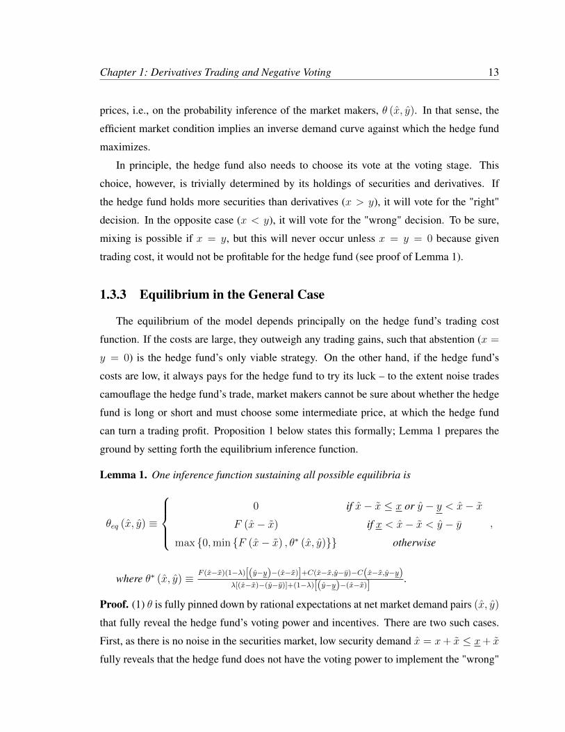
1.3.3 Equilibrium in the General Case

The equilibrium of the model depends principally on the hedge fund’s trading cost

function. If the costs are large, they outweigh any trading gains, such that abstention (x =

y = 0) is the hedge fund’s only viable strategy. On the other hand, if the hedge fund’s

costs are low, it always pays for the hedge fund to try its luck – to the extent noise trades

camouflage the hedge fund’s trade, market makers cannot be sure about whether the hedge

fund is long or short and must choose some intermediate price, at which the hedge fund

can turn a trading profit. Proposition 1 below states this formally; Lemma 1 prepares the

ground by setting forth the equilibrium inference function.

Lemma 1. One inference function sustaining all possible equilibria is

θeq (x, y) ≡

0 if x− x ≤ x or y − y < x− x

F (x− x) if x < x− x < y − ymax {0,min {F (x− x) , θ∗ (x, y)}} otherwise

,

where θ∗ (x, y) ≡ F (x−x)(1−λ)[(y−y)−(x−x)]+C(x−x,y−y)−C(x−x,y−y)λ[(x−x)−(y−y)]+(1−λ)[(y−y)−(x−x)]

.

Proof. (1) θ is fully pinned down by rational expectations at net market demand pairs (x, y)

that fully reveal the hedge fund’s voting power and incentives. There are two such cases.

First, as there is no noise in the securities market, low security demand x = x+ x ≤ x+ x

fully reveals that the hedge fund does not have the voting power to implement the "wrong"


decision (x < x), and hence θ = 0. Second, as the amount of noise in the derivatives market

is limited, observed net demand y puts bounds on the possible hedge fund trades and may

reveal that the hedge fund strictly prefers the "wrong" or the "right" decision. In particular,

if derivatives demand is sufficiently low relative to securities demand (y < y + x − x),

it is clear that even with low noise trader demand the hedge fund could not possibly have

acquired more derivatives than securities (y = y − y ≤ y − y < x− x = x). In this case,

the hedge fund clearly strictly prefers the "right" decision, which will hence be adopted,

so θ = 0. A symmetric argument shows that θ = F (x− x) if derivatives demand is

sufficiently high (y > y + x − x) to reveal that the hedge fund will use all its power

(F (x− x)) to implement the "wrong" decision.

(2) At other market demand pairs (x, y), θ can w.l.o.g. be set to equate expected hedge

fund profits for the two trades that could have generated this demand, namely(x− x, y − y

)(such that x ≤ y – a "short trade") and (x− x, y − y) (such that x ≥ y – a "long trade"),

truncated at the outer bounds of rationally possible beliefs, namely 0 and F (x− x).

(a) For market demand pairs that are actually observed in a mixed equilibrium, this is

in fact the only θ consistent with equilibrium because in order to mix, the hedge fund must

be indifferent between the underlying long and short trades. For off equilibrium demand

pairs, setting market makers’ subjective off-equilibrium beliefs at this level achieves maxi-

mum "deterrence" of deviations from equilibrium (because at other values, either the long

or short deviation would be more profitable). Finally, no pure strategy equilibrium can ever

generate such market demand pairs (x, y) because the only possible pure strategey equilib-

rium is (0, 0), for which x fully reveals that x = 0 ≤ x; at other pure strategies, the hedge

fund would incur trading cost without being able to make a trading profit because its voting

power and incentives are fully known and hence the hedge fund pays for the derivatives

and securities exactly what it expects to get out.

(b) Truncation is immaterial because where truncation occurs, both long and short prof-

its are negative with or without truncation, such that the hedge fund would not place the

corresponding trades in either case. Consider first truncation at θ = 0. For the long trade

(x ≥ y), expected profits (λθ [(x− x)− (y − y)]−C (x− x, y − y)) are negative at θ ≤ 0


(recall that the only cases considered here have x > x ≥ 0, such that C (x, y) > 0).5 Thus

if equality of profits for long and short trades occurs at θ ≤ 0, both profits are negative at

that θ. But then profits for the short trade ((1− λ) [F (x− x)− θ][(y − y

)− (x− x)

]−

C(x− x, y − y

)) must also be negative at θ = 0 because short profits are decreasing in θ.

The argument for upper truncation at F (x− x) is symmetric.

(c) θ∗ equates profits for the long and short trades, i.e., θ∗ solves λθ [(x− x)− (y − y)]−C (x− x, y − y) = (1− λ) [F (x− x)− θ]

[(y − y

)− (x− x)

]− C

(x− x, y − y

).

Briefly, the reasoning behind θeq is as follows. First, some market demand realizations

(x, y) fully reveal the hedge fund’s incentives, such that θ must be equal to 0 or F (x− x),

as the case may be (the hedge fund’s voting power can always be inferred from market

demand because liquidity traders’ demand for securities x is non-stochastic). Second, at

other market demand realizations, defining θeq to equate expected hedge fund profits from

the long and short trades that could generate this (x, y) sustains mixing if these are equilib-

rium trades, and optimally deters deviations if these are off-equilibrium trades.

Proposition 1. The hedge fund’s equilibrium (expected) profits are max {0, π∗}, where

π∗≡maxω π(x,y),ω≡{(x,y)|x>x, y∈[x−δ,x]}

and

π(x,y)≡F (x)λ(1−λ)(x−y)(y+δ−x)−λ(x−y)C(x,y+δ)−(1−λ)(y+δ−x)C(x,y)λ(x−y)+(1−λ)(y+δ−x)

The hedge fund’s equilibrium strategies depend on π∗:

(a) If π∗ < 0, the unique equilibrium is for the hedge fund not to trade at all (x = y =

0).

(b) If π∗ > 0, any strategy such that∑

(x∗,y∗)∈arg maxω π(x,y) [σ (x∗, y∗) + σ (x∗, y∗ + δ)] =

1 and σ (x∗, y∗) > 0 ⇒ σ(x∗,y∗)σ(x∗,y∗+δ)

= 1−λλ

[F (x∗)

θ∗(x∗+x,y∗+y)− 1]∀ (x∗, y∗) ∈ ω is an equilib-

rium; the equilibrium is unique if and only if arg maxω π (x, y) is unique.

(c) If π∗ = 0, any linear combination of (a) with strategy profile (b) is an equilibrium.

Proof. By construction, π∗ coincides with the highest non-negative expected profit, if

5The economic reason is that long trading profits derive from misleading the market into thinking that the"wrong" decision may be taken (θ > 0), the more the better.


any, that the hedge fund can obtain from trades (x, y) ∈ ω given θeq, since π (x, y) =

λ (x− y) θ∗ (x+ x, y + y)−C (x, y) coincides with Ey [Π (x, y; θeq (·, ·)) | (x, y) ∈ ω] un-

less θeq is truncated, which only occurs where expected profits are negative (see part (2)(b)

of the proof of Lemma 1). The maximum π∗ exists because π is a continuous function

on the closed interval ω. Any trade (x∗, y∗) generating π∗ – and the trade (x∗, y∗ + δ),

which yields identical profits by construction of θ∗ – will (strictly) dominate not trading

(x = y = 0) if π∗ is (strictly) greater than zero; otherwise not trading strictly domi-

nates. If more than one trade generates π∗, the hedge fund is indifferent between them

and can mix them in any proportion. Mixing optimal trade pairs ((x∗, y∗) , (x∗, y∗ + δ))

in the stated proportions ensures that θeq (x∗ + x, y∗ + y) = θeq(x∗ + x, y∗ + δ + y

)=

F (x∗)(1−λ)σ(x∗,y∗+δ)(1−λ)σ(x∗,y∗+δ)+λσ(x∗,y∗)

= Pr (v = 0|x, y) is correct. If the hedge fund does not trade, the

inference θeq(x, y)

= θeq (x, y) = 0 is correct because the hedge fund will not be able to

influence the decision, so Pr (v = 1|x, y) = 1.

It remains to be shown that only trades (x, y) ∈ ω need to be considered in the search

for a profitable trade. Given the inference function θeq, the hedge fund’s trading profits

are zero regardless of the noise realization unless x − δ ≤ y ≤ x + δ and x > x, and

thus expected profits for such trades are negative given positive trading costs.6 Moreover,

by construction (see proof of Lemma 1), θeq ensures that for each trade (x, y) such that

x < x ≤ y ≤ x + δ, there is a corresponding trade (x, y − δ) ∈ ω that yields equal

expected profits unless expected profits for both trades are negative.

Corollary 1. There always exists a non-zero cost function C (·, ·) such that a mixed equi-

librium exists.

Proof. If C (x, y) = 0 ∀ (x, y), then π∗ = maxωF (x)λ(1−λ)(x−y)(y+δ−x)λ(x−y)+(1−λ)(y+δ−x)

> 0. The proof then

follows by continuity of π (·, ·;C (·, ·)) in C (·, ·).

6Regardless of the noise realization, trading profits are (x− y) θ (x+ x, y + y) = (x− y) · 0 = 0 ify < x−δ, (y − x) [F (x)− θ (x+ x, y + y)] = (y − x) [F (x)− F (x)] = 0 if y > x+δ, and (x− y) ·0 =(y − x) (0− 0) = 0 if x ≤ x.


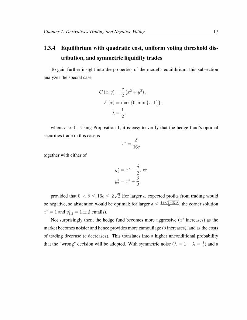
1.3.4 Equilibrium with quadratic cost, uniform voting threshold dis-

tribution, and symmetric liquidity trades

To gain further insight into the properties of the model’s equilibrium, this subsection

analyzes the special case

C (x, y) =c

2

(x2 + y2

),

F (x) = max {0,min {x, 1}} ,

λ =1

2,

where c > 0. Using Proposition 1, it is easy to verify that the hedge fund’s optimal

securities trade in this case is

x∗ =δ

16c

together with either of

y∗1 = x∗ − δ

2, or

y∗2 = x∗ +δ

2,

provided that 0 < δ ≤ 16c ≤ 2√

2 (for larger c, expected profits from trading would

be negative, so abstention would be optimal; for larger δ ≤ 1+√

1−32c2

2c, the corner solution

x∗ = 1 and y∗1,2 = 1± δ2

entails).

Not surprisingly then, the hedge fund becomes more aggressive (x∗ increases) as the

market becomes noisier and hence provides more camouflage (δ increases), and as the costs

of trading decrease (c decreases). This translates into a higher unconditional probability

that the "wrong" decision will be adopted. With symmetric noise (λ = 1 − λ = 12) and a


unique trading equilibrium, this probability is

Pr (v = 0) = F (x∗)σ (x∗, y∗2)

=F (x∗) (1− λ)σ (x∗, y∗2)

(1− λ)σ (x∗, y∗2) + λσ (x∗, y∗1)

= θeq(x∗ + x, y∗2 + y

)=

δ

16c

(1

2− 2c

).

This is increasing in the amount of "noise" or demand fluctuation, δ, and decreasing in

the trading cost or market illiquidity, c. The liquidity traders’ trading losses δ2

128c(1− 4c)

are also increasing in the amount of "noise" or demand fluctuation, δ, and decreasing in the

trading cost or market illiquidity, c.

At least in this special case, the model therefore shows that increasing liquidity (c) and

market size (δ) aggravate the problem analyzed in this paper.

1.3.5 Multiple Hedge Funds

Explicitly modelling the interaction of multiple hedge funds is far from straightforward,

and will not be attempted here. As hinted above in subsection 1.3.1, however, one can

at least state that problems of negative voting would persist in the presence of multiple

strategic traders:

Corollary 2. Regardless of the number of hedge funds, the equilibrium x = y = 0 exists if

and only if π∗ < 0.

Proof. If π∗ ≤ 0 and market makers’ inference function is θeq, no individual hedge fund

can profitably deviate by trading, while market makers correctly infer that the possibility of

the "wrong" decision being adopted is zero. Conversely, if π∗ > 0, then any one hedge fund

would be better off trading regardless of the inference function (recall that θeq minimizes the

maximum possible trading profit), so x = y = 0 cannot be an equilibrium. The presence of

other non-trading hedge funds is irrelevant to this argument.


1.4 Discussion

This section considers economic and legal constraints that curtail over-hedging and

negative voting. In particular, the section explains why the problem is much more likely

to arise with derivatives than with alternative, more traditional hedges, what "natural" and

regulatory barriers currently limit the problem, and in which situations the problem is there-

fore most likely to manifest. It argues that the problem is likely to be most acute in out-

of-bankruptcy restructurings and freezeouts, which can be blocked by a relatively small

minority stake, and arguably legally so.

1.4.1 Derivatives vs. other hedges

The first question to ask is why over-hedging is specifically a problem of derivatives.

In principle, over-hedging can occur with any investment that is negatively related to the

shares or debt at issue. Some examples include parallel investments in competing firms,

parallel investments in both the acquiror and the target of a merger transaction, parallel

investments in different securities of the same firm, or selling short some amount of a

security while holding on to a smaller amount. These other investments, however, are either

not perfectly correlated with the shares or debt and hence represent higher risk, or they are

only available in particular situations, or they are available only in small quantities or at

higher cost, or all of the above. These shortcomings severely limit the facility, frequency,

and extent to which these other investments could enable over-hedging.

By contrast, derivatives are designed to be perfectly (negatively) correlated with the

payoffs of shares or debt. Many derivatives markets, such as those for equity options,

are highly liquid at all times. Even those that are not, such as single-name CDS, exhibit

liquidity spikes around key events when over-hedging is most profitable, such as changes

in credit outlook for CDS (Chen et al. 2011). In general, the rapid growth of derivatives

markets over the last decade or two means that derivatives are in principle available in high

volumes at low prices (spreads). It is not unusual that the face amount of derivatives written

on the shares or debt of an individual company exceeds the amount of shares or debt issued

by that company (Stulz 2010).


1.4.2 Required control stakes

Even if derivatives are available, it might seem an implausible proposition to acquire

and over-hedge a voting majority (51%) of a corporation’s shares or publicly traded debt.

Such quantities of shares/debt and derivatives may not even be available on the market, and

if they were, could hardly be acquired in secret and without strongly affecting prices. For

shares, acquiring such quantities would also trigger disclosure and other obligations under

corporate and securities laws and, in most U.S. corporations, the “poison pill.”7

Many relevant decisions, however, can be affected by much smaller percentages of

shares or debt. One possibility is that an over-hedged shareholder or creditor joins forces

with some other constituency pursuing interests other than maximizing share or debt value,

such as a corporate insider.

More importantly, some corporate decisions provide blocking power to relatively small

minorities. In particular, out-of-bankruptcy restructurings tend to set acceptance thresh-

olds around 95%, providing blocking rights to 5% or even less of the outstanding debt.

Importantly, restructurings that do not bind all holders, such as a standard debt exchange,

do not constitute a credit event under the prevailing CDS documentation and hence do not

trigger settlement of the CDS; this may amplify the incentives for negative voting because

bankruptcy accelerates payment.8 Practitioners suspect that over-hedging and negative vot-

ing are common in out-of-bankruptcy restructurings.9 In addition to restructurings, small

stakes may be sufficient to affect freeze-out mergers. Majority-of-the-minority conditions

in freeze-outs can give blocking rights to as little as a few percent of the corporation’s

outstanding equity.10

7See in particular section 13(d) of the Exchange Act, which requires disclosure of equity ownership stakesabove 5% and arguably of any hedges relating thereto (cf. discussion in the next section), and section 16 ofthe Exchange Act, which forces 10% shareholders to disclose their hedges (sec. 16(a)) and disgorge short-swing trading profits (sec. 16(b)). Moreover, section 16(c) prohibits 10% shareholders from engaging inshort sales, and rule 16c-4 explicitly extends this to over-heding using puts, while they are a 10% shareholder,thus outlawing any strategy of acquiring a voting stake first and over-hedging it later (but not the other wayaround).

8Cf. Art. 4.7(a) of the 2003 ISDA Credit Derivative Definitions, as amended by the "Small Bang Proto-col," available at http://www.isda.org/publications/pdf/July-2009-Supplement.pdf.

9Author’s conversation with the head of the restructuring practice of a major New York law firm.

10Such majority-of-the-minority conditions have been imposed by Delaware courts as a condition for ob-


1.4.3 Legal constraints

At least in the U.S., current law only provides incomplete protection against over-

hedging and negative voting. With respect to formal voting, U.S. law arguably provides

some protection, but enforcement may be hindered by a lack of disclosure. Outside of

formal voting, negative voting and over-hedging are arguably entirely unregulated.

Under §1126(e) of the U.S. Bankruptcy Code, bankruptcy judges have the power to

disallow votes by a creditor “whose acceptance or rejection of [a reorganization] plan was

not in good faith.” In a recent decision, the U.S. Bankruptcy Court for the Southern District

of New York held, obiter, that this provision would justify disqualification of votes by over-

hedged creditors.11 Bankruptcy courts will generally not know, however, if creditors are

over-hedged. Current bankruptcy rules do not require disclosure of hedging transactions

relating to debt claims filed in the bankruptcy.

For shares, the Delaware Supreme Court recently recognized “[a] Delaware public pol-

icy of guarding against the decoupling of economic ownership from voting power.”12 There

is thus reason to believe that Delaware courts would at least seriously consider a remedy

against voting by over-hedged shareholders. Section 13(d)(1)(E) of the Exchange Act ar-

guably requires that owners of 5% or more of a corporation’s stock disclose hedging trans-

actions, but in practice market participants have not done so effectively. To address the

enforcement problem, commentators have advocated stricter disclosure obligations. For

example, Hu and Black (2006, 885) argue that voting by over-hedged shareholders or cred-

itors above a threshold of 0.5% of a company’s shares or debt should be reported.

Neither of these rules or proposals, however, deals with the exercise of control rights

other than formal voting rights. In particular, no rule forces an over-hedged creditor to

participate in a debt exchange, even if the over-hedging were publicly known. In freeze-out

tender offers, the Delaware Chancery Court has excluded votes by hedged shareholders for

taining favorable review of the consideration paid to the minority, see In re Cox Communications Inc. Share-holders Litigation 879 A.2d 604 (2005); In re CNX Gas Corp. Shareholders Litigation, 4 A.3d 397 (Del. Ch.2010).

11In re DBSD North America, Inc., 421 B.R. 133, 143 n. 44 (Bankr. S.D.N.Y. 2009).

12Crown Emak Partners, LLC v. Kurz, 992 A.2d 377, 387 n. 17 (Del. 2010).


purposes of a majority-of-the-minority condition.13 These decisions are based on fiduciary

duties of the board and parent shareholders, however, and it is not clear that they would

extend to situations in which the hedged shareholder stands in opposition to the board and

the parent. In particular, the Court has affirmed that even controlling shareholders are under

no obligation to sell their shares, even if doing so might be beneficial to other shareholders

or the corporation.14

1.5 Conclusion

This paper has shown theoretically that derivatives can create opportunities for purely

value-reducing activity (over-heding and negative voting) if derivative traders can conceal

their overall positions from their counterparties. It has also argued that the institutional and

legal conditions in the US are such that the threat of such activity seems real at least in

out-of-bankruptcy restructurings and freezeout mergers.

This assessment of the role of derivatives is considerably less benign than that of other

papers that have assumed no assymetric information in the relationship between derivative

counterparties, in particular Bolton and Oehmke (2011) and Campello and Matta (2012).

Determining which assumption better describes the derivative market, or rather which parts

of that market correspond to which assumption, seems an important area for future research.

In as much as regulatory reforms push derivative trading into anonymous exchanges and

hence closer to the assumptions of the present paper, it would be worth considering flanking

measures to guard against the problems discussed here.

13See In re CNX Gas Corp. Shareholders Litigation, 4 A.3d 397, at 418 (Del. Ch. 2010); In re PureResources, Inc., Shareholders Litigation, 808 A.2d 421, at 426 and 446 (Del. Ch. 2002).

14Cf. In re Digex, Inc. Shareholders Litigation, 789 A.2d 1176, 1189-91 (Del. Ch. 2002) (noting that acontrolling shareholder is free to block the sale of the controlled corporation to another bidder by not selling).

Chapter 2

American Exceptionalism Revisited:

The Global Cross-Section of Crime and

Punishment

2.1 Introduction

The United States exhibits astonishingly high crime and punishment among developed

countries. For example, in 2004, the WHO recorded 5.9 murders per 100,000 inhabitants

in the US, but only 0.8 in France (WHO 2009). Incarceration rates – measured as inmates

per 100,000 inhabitants – now range from the global maximum of 751 in the US to 91 in

France to 36 in Iceland (ICPS 2008). And the United States is one out of only two OECD

countries that continue to apply the death penalty (Anckar 2006). Moreover, as shown in

the little table below, Table 2.1, some of these differences appear to be long-lasting. For

example, while the US prison population per capita has increased almost five-fold since

1974, it was already seven times higher than France’s in 1974, a similar relative difference

as today. Even the dramatic drop in US crime during the 1990s by about 40% (Levitt 2004)

is small relative to these cross-country differences.

Understanding the drivers of these differences is immensely important. While the wel-

fare losses imposed by crime and punishment are hard to estimate, they are surely substan-

23

Chapter 2: American Exceptionalism Revisited: The Global Cross-Section of Crime andPunishment 24

Table 2.1:

US Canada UK France Germany Japanhomicides per 100,000, 2004a 5.9 1.4 2.0 0.8 0.7 0.5prisoners per 100,000, 2004b 751 108 149 91 88 63id., 1974-75c 162 109 66 24 57 34death penalty, 2007d Yes No No No No Yesasources: WHO 2009; b ICPS 2008; c 1st UN World Crime Survey, revised,and WDI; dAmnesty International 2008

tial. For example, just the life expectancy reduction due to homicides is valued by Soares

(2004b) at 0.9% of US GDP, and 9.7% of Colombian GDP in 1995. In the United States,

the prison population now comprises 1% of the adult population, and combined with pro-

bation and parole, 3.2% of US adults are under some form of correctional control (PEW

Center for the States 2009).1 The out-of-pocket costs of US correction departments alone

are close to US$ 50bn, which impose a significant burden on state budgets (Steinhauer

2009).

In this paper, I assemble the literature’s largest data set of crime and punishment around

the world to inquire if commonly theorized country characteristics can explain the afore-

mentioned differences in crime and punishment, and in particular the US outlier position.

Briefly, the answer is that while US crime rates are not exceptional given US income in-

equality and family structure, US incarceration rates are an order of magnitude higher than

what any commonly mentioned measurable factors would predict. I find that of all the

major variables suggested in the cross-country literature on crime and punishment, only

lower levels of development, income inequality, and current teen birth rates are robustly as-

sociated with more crime, while only moderate levels of development, common law legal

systems, and (formerly) socialist systems are robustly associated with more prisoners; com-

mon law systems are also more likely to retain the death penalty. Muslim societies appear

to have less crime and harsher punishment. I find no cross-sectional support for links be-

tween democracy and crime (Lin 2007), or between children of teenagers and crime (Hunt

1For some reviews of the human tolls behind these numbers, see Clear (2008) and Murray and Farrington(2008).


2006). Outside the richest countries, I also find no support for criminological theories

linking incarceration rates to political structure and social policy.

My approach of exploiting the largest possible cross-country sample consciously de-

parts from most of the comparative criminological literature, which tends to study much

smaller groups of developed countries (e.g., Tonry and Farrington 2005 [7 countries];

Lappi-Seppälä 2008 [up to 25 countries]). Such studies are very valuable because they

can exploit a wealth of detailed data that is not available for larger samples, and because

they consider many subtle theories that, realistically, a cross-country regression cannot.

Yet they stand to benefit from being complemented with large-N cross-country studies for

several reasons, even if that means enlarging the sample to less developed countries. First,

the determinants of crime and punishment in less developed countries are of interest in

their own right. Second, many of the theories used to explain incarceration rates in small

developed world samples have no obvious limitation to developed countries, and some,

such as the "civilization" theory of punishment, would appear to be particularly apt at ex-

plaining differences between developed and developing countries. Third, and perhaps most

importantly, constant focus on the same few data points inevitably leads to "retrofitting"

of theories to the data, and calls for out-of-sample tests using additional countries. As a

robustness check, I also present results for only OECD and EU member states.

The primary data sets that I use are comparably high quality data on homicides in

2004 in 190 countries (WHO 2009), the number of prisoners around 2007 in 214 countries

(ICPS 2008), and the use of the death penalty in 2007 in 195 countries (Amnesty Inter-

national 2008). In addition, I pool data from multiple rounds of the International Crime

Victims Survey to obtain data on smaller crimes in 74 countries from 1989 to 2005, and

use some other data for robustness checks. I regress these measures of crime and pun-

ishment on all major explanatory variables that have been suggested in the comparative

literature. For the econometric reasons explained in section 2, I do not control for crime

in the punishment regressions and vice versa. This approach does not promise insight into

the crime-punishment nexus, but it does promise insight into the drivers of both. To deal

with the degrees-of-freedom problem of an overabundance of theories purporting to explain

comparative crime and punishment, I initially focus on small, related blocks of explanatory

variables at a time in the belief that any relationship of first-order importance should mani-


fest itself in a simple setup controlling only for the level of development. In a second step,

I run against one another those variables that cleared the first hurdle (defined as a t-statistic

of at least 1.64).

While there is already a small regression literature on crime and punishment (see sec-

tions 3 and 4 below), this paper differs in at least one of the following four respects from that

prior work. First, most papers work with smaller samples. I am aware of only three papers

(Neapolitan 2001; Anckar 2006; Greenberg and West 2008)2 that exploit the full available

sample of punishment data (prisoners counts, and application of the death penalty), and

none that exploits the full sample of WHO and ICVS crime data. Second, many papers

control for a measure of punishment in crime regressions, and vice versa. As discussed in

more detail in Section 2, however, this approach yields estimates that are hard to interpret,

since they correspond neither to structural nor reduced form equations of crime and pun-

ishment conditional on a set of background variables. Third, and relatedly, this paper is the

only one to study crime and punishment in parallel. This is important for the interpretation

of coefficients. In particular, it might be tempting to interpret a positive correlation of some

background factor with higher incarceration rates as evidence that that background factor is

associated with higher "punitiveness." This interpretation is much less plausible, however,

if it turns out that the background factor is also associated with higher crime rates, such that

prisoner rates per crime may actually be lower. Fourth, only one other paper (Greenberg

and West 2008) studies the impact of legal origin on punishment policies. Finally, some

papers work with panel data. While this approach presents certain distinct advantages

over purely cross-sectional approaches, it also has some considerable disadvantages in the

comparative context, since many of the relevant explanatory variables such as democracy

or income inequality vary relatively little over time, and limited data availability for past

decades forces panel approaches to work with far fewer countries and lower quality data.

The rest of the paper is structured as follows. Section 2 explains in more detail the

rationale for focusing on reduced form equations in the comparative context. Section 3

introduces the dependent variables, and Section 4 the independent variables and the theories

behind them. Section 5 describes the specifications that I run. Section 6 presents and

2Ruddell (2005) uses the same incarceration data, but restricts the sample to the richest 100 countries.


discusses the results. Section 7 reports robustness checks. Section 8 presents further results

for a surprisingly strong predictor of punishment, legal origins, and discusses the possible

theory behind it. Section 9 concludes.

2.2 Structural vs. reduced form equations

In this section, I set out in more detail the rationale for focusing on reduced-form equa-

tions of crime and punishment, respectively. The basic problem – simultaneity of crime and

punishment – is in principle well understood (e.g., Levitt and Miles 2007; Spelman 2008).

Yet the implications of the problem for cross-country regression specifications are often

not recognized. In particular, many researchers interested in the cross-country relationship

between punishment and some background social variable, such as inequality, include a

measure of crime as a control variable in an effort to "hold crime constant."3 This is par-

ticularly tempting in explorations of "punitiveness," i.e., punishment per crime, because

raw incarceration rates confound punitiveness and the mechanical effect of the crime rate

on incarceration, holding punishment constant.4 Given the simultaneity problem, however,

including a control for "crime" does not identify a structural equation, nor does it capture

the full effect of the background variable on punishment because some of that effect may

come through an effect on crime.

2.2.1 A simple model of the simultaneity problem

To make this clearer, to discuss what can or cannot be estimated, and to provide con-

ceptual clarity for the specifications actually estimated below, it is useful explicitly to set

out the stylized model that underlies all cross-country regressions in the area of crime and

3There are also studies of the cross-country determinants of crime that use measures of law enforcementas right-hand side variables, but the authors are aware of the endogeneity problem and treat the estimates aslower bounds and/or robustness checks (e.g., Soares 2004, 166n.6; Hunt 2006, 552).

4Listokin (2006) verifies the mechanical crime-prisoner relationship empirically using US data. The rightway to account for this effect, however, would be to modify the dependent variable by dividing it by the crimerate, i.e., to use prisoners per crime rather than prisoners per population as the dependent variable (Blumsteinet al. 2005; cf. Pease 1994). On the econometric problems of this approach, see subsection 2.2 below.


punishment. The model has a unitary concept of crime, C, and a unitary concept of punish-

ment, P , which at least implicitly is defined as punishment per crime.5 Individuals choose

their level of criminal activity given (expected) punishment P and background conditions

X:

C = f (P,X, ε) ,

where the error term ε includes factors omitted from X and P . P in turn is derived en-

dogenously from a policy-maker’s choice P ∗ plus error η. P ∗ trades off the costs of crime

and the costs of punishment, where X enters the analysis as an index of the objective func-

tion U (·) (as budget constraints, social preferences, etc.), while the error term η accounts

for implementation problems, delays, political frictions, etc.:

P = P ∗ + η = arg maxP ′

U (f (P ′, X, ε) , P ′;X) + η = g (X, ε, η) .

Two structural equations are commonly discussed in the literature: the crime equation,

f (·), and a measure of "punitiveness," which I understand to mean ∂P ∗

∂X|C . In general,

however, simple cross-sectional regressions cannot yield unbiased estimates of either of

the two equations, given the correlation of P and C with X , ε, and η through the system of

equations C = f (P,X, ε) and P = g (X, ε, η).

2.2.2 The absence of valid instruments

To estimate the structural equations with instrumental variables, some elements of X

would need to be excludable from one of the two equations. As the theory review in Section

4 below will show, however, almost all variables of interest have potential direct effects on

both crime and the choice of punishment. In particular, all variables that have a plausible

effect on the choice of punishment given crime may also belong into the crime equation

5A full model would decompose P into the probabilities of prosecution and conviction, the length of theprison term if convicted the severity of prison conditions, etc. It would also distinguish different categoriesof crime and associated punishment, i.e., P and C would be vectors.


directly.6

As a theoretical matter, some variables, such as the age structure of society, may be

excludable from the punishment equation. As a practical matter, however, a more subtle

problem relating to measurement error and the available data prevents estimation of the

punishment equation using these variables as instruments. The source of the problem is that

direct comparative measures of P , such as the sentence meted out for some particular crime,

are conceivable but do not currently exist for larger samples.7 In the absence of a direct

measure, one could think of using incarcerationratecrimerate

= prisoners/populationcrime/(population∗year)

ss= E

[prisontimecrime

]as a measure of P . This would work well in the simple model above with unitary concepts

C and P , or with incarceration and crime rates by type of crime i, such that one could

construct Pi = incarcerationrateicrimeratei

. Given data limitations, however, one would per force

divide the general incarceration rate, which is the only one available, by the crime rate for

a particular crime. This introduces noise because the relative frequency of types of crimes

is likely to differ by country. This noise will be correlated with variables that affect the

relative frequency of certain crimes. Hence these variables cannot be used as instruments

in practical empirical specifications of the punishment equation even though they may be

theoretically excludable from the structural equation. An example is the teen birth rate,

which is strongly positively correlated with the relative frequency of homicide.

2.2.3 Reduced-form equations

What can one estimate with simple cross-sectional OLS? First, one can estimate a

reduced form equation for crime, namely E∗ [C|X]. To be more precise, one estimates

E∗ [Ci|X] for particular crimes i for which we have reliable measurements (see section

3.1 below). Second, one can estimate a reduced form equation of the incarceration rate,

E∗[prisonerspopulation

|X]

= E∗ [PC|X].8 This variable is also particularly well measured, and

6Soares (2004, 166n.6) also notes that it was not possible to find a good instrument for, in his case, thenumber of policemen in the comparative context.

7Lin (2007) uses measures of average prison length per crime, and prisoners per crime, from the UNCrime Trend Survey. These data, however, are only available for small groups of countries, and lackingstandardized definitions of crimes, are likely not very reliable.

8With different types of crime, P and C are vectors, with elements pi and ci, respectively, for crime i.


therefore deserves considerable attention. Finally, to the extent that the existence of the

death penalty is a valid measure of punitiveness, one can estimate a reduced form equation

of E∗ [P |X] using death penalty data. In this paper, I pursue all three options.

2.3 Dependent Variables

This section describes the data used as dependent variables in this paper.

2.3.1 Crime

Reliably measuring crime is notoriously difficult, since much crime is not reported.

Importantly, the propensity to report crime covaries with certain variables of interest, such

as the level of development or inequality, so that official crime data will paint a very mis-

leading comparative picture (Soares 2004; Gibson and Kim 2008). INTERPOL (1999)

explicitly warns against using its data for comparative purposes.

WHO homicide rate.

There are two series of crime data, however, that are considered reliable, and I use both

of them in this paper. The first is the homicide rate, because homicides are less easily

concealed. There are two comparative data series in wide use, UNODC data from police

statistics, and WHO data from death classifications by medical practitioners (Newman and

Howard 1999). I use the latter, as reported for 2004 (WHO 2009), because it has substan-

tially greater country coverage (N = 192). By comparison, the latest UNODC data (also

for 2004) is available for only 66 countries; the correlation between the two data series is

.72).

ICVS prevalence rates for common crimes.

The second reliable series of crime data come from victimization studies, i.e., repre-

sentative surveys eliciting experiences of victimization by various crimes (Tonry and Far-

rington 2005; Lynch 2006). Standardized comparative data on ten common property and


contact crimes have been collected in five sweeps of the International Crime Victims Sur-

vey between 1989 and 2005, including the European Survey on Crime and Safety (van

Dijk, van Kesteren, and Smit 2007; van Kesteren 2007) (hereinafter collectively referred to

as ICVS).

The major shortcoming of these data is low coverage in any given sweep. Although 74

countries participated in at least one of the five sweeps, any given sweep covered far fewer.

For example, the 2004-05 sweep contained only 27 country surveys (essentially all and

only OECD countries). Consequently, papers using these measures in the past have had

only about 40 observations to work with (e.g., Soares 2004). To my knowledge, I am the

first to pool data from all five sweeps, including city surveys from developing countries,

which gives me 74 countries or around 300,000 individual responses (after eliminating

duplicates) to work with. (I take appropriate steps to adjust for the unbalanced nature of

the data, see Section 5.2 below.)

I use the one-year prevalence rate of victimization by any of nine common crimes (bur-

glary; attempted burglary; personal theft; theft of a car, theft from a car; theft of a bicycle;

theft of a motorcycle; assault; and robbery), i.e., the probability of being the victim of

any of these nine crimes at least once in the year before the survey.9 This measure is com-

monly emphasized in the comparative literature as a proxy for overall crime (e.g., van Dijk,

van Kesteren, and Smit 2007), it has sufficiently many non-zero observations to estimate

country averages reliably, and its focus on less serious crimes provides a useful counterper-

spective to the homicide measure.

WHO drug-related death rate.

For robustness checks, I also use the rate of drug-related deaths per 100,000 in 2004 as

reported by the WHO (2009). I do so because of the common perception that the US prison

population is in large part driven by the "war on drugs," and so I want to have at least some

idea of whether factors that correlate with higher prisoner counts also correlate with lower

or higher visible effects of drug abuse.

9I do not include sexual offenses against women in this count because this question was not asked inall surveys, and in any event would presumably yield answers that are not necessarily comparable acrosscountries.


2.3.2 Punishment

For punishment data, I focus on the incarceration rate and the application of the death

penalty, which are very reliably measured. Punishment has additional dimensions, most

importantly prison conditions. At least in the developed world, however, the severity of

prison conditions and the size of prison populations seem to be strongly positively corre-

lated (Whitman 2003; Tonry and Melewski 2008), and so I did not explore this point further

in the absence of good comparative data.10

Incarceration rate. The main punishment variable I use is the incarceration rate per

100,000 inhabitants (= PC) in 2007 or latest available from the International Center for

Prison Studies at King’s College, London (ICPS, 2008), who collect these data mainly

directly from national prison authorities. The incarceration rate is conceptually straightfor-

ward and easily observed. While incarceration rates alone do not capture all dimensions of

punishment associated with prisons (Young and Brown 1993), they are at least a joint mea-

sure of the most important ones, admission rates and sentence lengths. The ICPS data are

considered highly reliable (Neapolitan 2001; Lappi-Seppälä 2008), and country coverage

is near to universal.11 For a robustness check, I also use historic incarceration rates from

the United Nations World Crime Survey, rounds 1 through 8.12

Application of the death penalty. In addition, I use a dummy variable from Amnesty

International (2008) indicating whether a country still applied the death penalty in ordinary

10Neapolitan (2001,695) constructs a measure of prison conditions from the US State Department’s Coun-try Reports on Human Rights Practices for 1994-98, "group[ing them] into three general categories: prisonconditions meet minimum international standards, prison conditions are harsh and do not meet minimuminternational standards, and prison conditions are harsh to the point of being life threatening." He finds thatharsh prison conditions correlate negatively with the level of development and freedom, and positively withincome inequality. The latter two effects go in the same direction as his findings for the incarceration rate.

11To match the data with other variables, I merge Guernesey and Jersey into Channel Islands, and Englandand Wales, Northern Ireland, and Scotland into the UK.

12The name of the survey and the organizing entity has changed over the years. The original surveys wereadministered under the auspices of the United Nations Criminal Justice and Crime Prevention Branch (for thefirst and second survey, I use revised and expanded data, see http://www.uncjin.org/stats/wcsascii/readme.txt).The latest rounds are administered by the United Nations Office of Drugs and Crime, and the survey is nowcalled the "United Nations Survey of Crime Trends and Operations of Criminal Justice Systems."


criminal cases in 2007 at least in principle, even though it may not have carried out execu-

tions in 2007. These data are widely used in the literature (e.g., Anckar 2006; Greenberg

and West 2008). According to Amnesty International, there were 60 such countries in 2007,

out of 196 countries covered. If I used instead the number of executions, I would have only

24 non-zero observations (only 17 of which had more than one confirmed execution).

2.4 Independent variables

As independent variables, I attempt to use all of the main variables suggested in the

comparative literature on crime and punishment, in as far as they are amenable to testing

in the large cross-section and are not simultaneously determined with crime and punish-

ment.13 In particular, and subject to the previous caveat, I use all of the variables suggested

in the cross-country regression literature on crime (Messner, Raffalovich and Shrock 2002;

Fajnzylber, Lederman and Loayza 2002; Soares 2004; Hunt 2006; Lin 2007) and punish-

ment (Neapolitan 2001; Jacobs and Kleban 2003; Ruddell 2005; Anckar 2006; Downes

and Hansen 2006; Greenberg and West 2008), or close substitutes thereof. The theoretical

literature motivating these variables is voluminous; for excellent reviews, see Neapolitan

(1997), Whitman (2005), Tonry (2007), and Lappi-Seppälä (2008). Here I only give very

brief descriptions of each variable and its possible relevance. Summary statistics for all

variables are shown in Table 2.2.

13Independent variables that have been used in the comparative literature but are almost certainly simul-taneously determined with crime and (official) punishment are extrajudicial killings (Neapolitan 2001), andcrime and official punishment themselves.


Table 2.2: Main variables: summary statistics

Variable Obs. Mean St. Dev. Min Max

Homicides per 100,000 pop., 2004 191 10.78 12.23 0 82.63 (Colom-

bia)

1-year victimization rate, various years 165 .24 .10 .08 .60 (Uganda)

Drug-related deaths per 100,000 pop., 2004 191 1.22 2.41 0 21.60

(Afghanistan)

Inmates per 100,000 pop., 2007 214 164.15 130.46 22 751 (USA)

Death penalty, 2007 195 .31 .46 0 1

GDP per capita, 2007 (1,000 dollars) 188 7.47 11.17 0.09 68.05

Legal origin 213

English .35

German .03

Scandinavian .02

Socialist .17

Muslim population 1980, % 201 21.16 35.05 0 99.90

Protestant population 1980, % 199 15.18 23.60 0 99.80

Catholic population 1980, % 201 33.27 36.35 0 99.10

Ethnic Fractionalization 181 .43 .26 0.00 .93

Freedom, 2007 189 .63 .32 0 1

Federalism, 2004 222 .11 .31 0 1

Proportional voting, 2006 148 1.41 1.31 0 3

% foreign-born pop., 2005 206 10.42 15.83 0.03 79.98

% of pop. living in urban areas, 2005 208 56.20 24.23 9.5 100

Males 15-19 / total pop., 2004 217 .047 .011 .022 .070

Teen mother births / total births, 1984-88 115 .11 .06 0.01 0.27

Difficulty of firing workers, 2007 178 31.35 22.76 0 100

Gini 131 40.66 9.45 24.70 74.33

Unemployment rate, 2005/06 103 9.68 7.53 1.30 40.45

Hofstede 65

PDI 58.63 22.04 11 104

IDV 44.11 24.35 6 91

MAS 50.69 19.06 5 110

Schwartz 51

Hierarchy 2.26 .50 1.41 3.63

Continued on next page


Table 2.2: Main variables: summary statistics

Variable Obs. Mean St. Dev. Min Max

Egalitarianism 4.81 .29 4.25 5.40

World Value Survey

Trust in people 83 .28 .15 .03 .67

Trust in police and parliament 79 .48 .11 .28 .87

Favor income inequality 71 5.89 1.15 3.54 8.24

Favor welfare state 80 5.77 1.07 3.26 7.86

Dislike competition 68 3.67 .57 2.47 4.80

Religious intensity 79 .73 .19 .15 .99

Since the sample overlap for different variables is imperfect, the actual samples in the regressions will differ from those shown

here. In addition, data used with the ICVS victimization data are year-matched to those data, and hence also different from

those shown here.

Some of the variables mentioned below could themselves be affected by crime and

punishment rates, particularly the level of development, unemployment, income inequality,

and social policy. I expect such effects to be small, but acknowledge that such concerns

could mar the interpretation of the results for those variables. At least for income inequality,

researchers have found that the link to crime is robust to methods controlling for potential

endogeneity (Fajnzylber et al. 2002).

Development. All of the aforementioned studies control for the level of development,

usually operationalized as GDP per capita.14 In fact, the impact of development is so

fundamental that presumably most other theories implicitly hold the level of development

constant, and I control for it in all of the regressions. The level of development affects the

opportunity set of potential criminals, and the institutional capacity of public law enforce-

ment. More subtly, the level of development may also affect social structures that infor-

mally suppress or encourage crime, and steer human behavior more generally. Finally, a

"civilization" effect may lead to less severe punishment in more developed societies. To

14Some authors, such as Neapolitan (2001), use instead the Human Development Index, which combinesGDP per capita, life expectancy, and educational achievement; I used it in some regressions with identical re-sults. Other authors, such as Soares (2004), separately include the level of education. I found that coefficientson a variable of primary school enrollment or adult literacy have the same sign as those for GDP per capita(less crime, more punishment) without adding explanatory power or altering the results for other variables.Since I do not see a theoretical reason for adding this separate variable, and to conserve degrees of freedom,I do not report results with this variable.


account for the possibility of the latter effect, I control for the level of development non-

linearly, using both the level of GDP per capita and its natural logarithm. With the ICVS

data, I use five-year PPP-adjusted averages around the survey date; with the other depen-

dent variables, I use 2007 raw data to maximize the sample size (using PPP-adjusted data

would lose as many as ten observations; the results are qualitatively identical). All the GDP

data come from the World Development Indicators.15

While researchers agree on the importance of development for some aspects of crime

and punishment, there is no agreement on the manifestation of this effect. In particular,

criminologists have often argued that development does not affect crime rates (e.g., Ruddell

2005:7), or even that development is criminogenic,16 and estimates by economists have

been unstable.17 Moreover, criminologists studying the relationship of development and

incarceration rates have reported mixed results.18 For both questions, the analysis of the

global cross-section thus promises to yield new insights.

Income inequality and social policy. Another major focus of the prior literature is in-

come inequality and the policies that influence it. The economic literature on crime mostly

emphasizes the effect of income inequality on the opportunity set of potential criminals

(e.g., Burdett et al. 2003). In the criminological and sociological literature on punishment,

income inequality is also viewed as a proxy for, and consequence of, social policies defin-

ing the relationship between the well-off and the less well-off, which are the major focus of

that literature. In that view, societies that support the poor with generous welfare spending,

and that support employees with protective labor regulation, are also likely to employ only

moderate punishment. I control for income inequality using the Gini coefficient from the

15To the raw GDP data, I also add data for Taiwan from the IMF Global Economic Outlook.

16Soares (2004) provides a full review of the relevant empirical literature.

17Soares (2004) and Hunt (2006) find no effect, while Lin (2007) find that the effect is negative for mostcrimes but positive for others (rape and car theft).

18Neapolitan (2001) and Ruddell (2005), using the Human Development Index, find no significant asso-ciation between development and incarceration rates, while Jacobs and Kleban (2003) and Lappi-Seppälä(2008), using GDP per capita, do find one. I have also run many of the reported regressions with the HumanDevelopment Index instead of GDP per capita, with similar results as those reported in this paper.


World Development Indicators (closest year available),19 and for labor regulation using the

World Bank’s Doing Business index of the ease of hiring and firing a worker for 2007 (this

index is not available prior to 2003, and so cannot be used with the ICVS data). Given

the difficulty of measuring welfare expenditures, the high correlation of available measures

with the Gini coefficient, and the fact that some Gini data already includes the effect of re-

distributive policies (Deininger and Squire 1996), I do not control for welfare expenditure

in the reported regressions; unreported regressions using welfare data from Gwartney and

Lawson (2007) found similar results as for income inequality, which mostly disappeared

after controlling also for income inequality directly.

Political structure. In the aforementioned criminological literature, differences in social

policy are usually viewed in a broader context of different political systems, and classifi-

cations such as corporatism (Jacobs and Kleban 2003), social democracies vs. neoliberal

systems vs. conservative corporatist systems (e.g., Cavadino and Dignan 2006a/b), or con-

sensus vs. conflict political systems (Lappi-Seppälä 2008) are directly included in the

analysis. Since these classifications are only available for relatively small groups of coun-

tries, however, I instead use a year-matched measure of proportional voting, which is often

viewed as conducive to, or even a hallmark of, social democracies or consensus systems.20

Relatedly, Lin (2007) and others have suggested that democracies punish minor crimes

less harshly and hence have more of it, and inversely for major crime. To control for

democracies and liberty more broadly, I combine the Freedom House political rights and

civil liberties scores for the relevant year, and rescale them so that higher values correspond

to more freedom.21

Finally, Jacobs and Kleban (2003) have argued that federal systems should have more

prisoners because relevant political decisions will be less remote from the population and

19In robustness checks, I also use the 10/10 and 20/20 income ratios. The results are similar but weaker.

20I construct the measure from the World Bank’s Database of Political Institutions (revision 4) using theformula of Pagano and Volpin (2005): PR - PLURALTY - HOUSESYS + 2.

21Lin (2007) uses the political rights score (and the civil liberties score as an instrument for it). Usingonly the political rights score does not change my results. Nor does using the Polity IV score instead of theFreedom House measures.


hence more subject to populist pressures for harsh punishment. I control for federalism

using a dummy variable derived from the Handbook of Federal Countries (2005).

Population structure. The last major complex of variables considered in the literature is

the structure of the population. It is well known that young males are particularly prone to

criminal activity (Hirschi and Gottfredson 1983), and many cross-country studies attempt

to control for this. I do so using the share of 15-19 year old males in the population in

2004, as reported by the US Census International Data Base.22 Hunt (2006) has drawn

attention to the particular importance of young adults born to teen mothers. I control for

this using the share of children born to teen mothers out of all children born 15 to 19 years

prior to the relevant year (2004 for homicide and the current imprisonment data, and the

survey year for ICVS data), calculated from the United Nations Demographic Yearbook

Historic Supplement 1948-1997.23 As I discuss later in the paper, this variable may be

a proxy for broader social dysfunctions, since the current share of teen births (calculated

from the same sources) correlates even more strongly with crime rates, and conditioning

on the current rate removes any correlation of the present rate with crime.

Many papers also control for the level of urbanization since crime tends to be more

prevalent in cities (Glaeser and Sacerdote 1999). I do so using the percentage of the popu-

lation living in urban areas in the relevant year (from World Development Indicators).

Another important aspect of population structure considered in the literature is its ho-

mogeneity or heterogeneity (e.g., Ruddell 2005). Group differences might breed conflict

and hence crime, and a government dominated by one group might have less reservations

about punishing members of the other group. To control for this, I use the index of ethnic

fractionalization from Alesina et al. (2003),24 and the percentage of foreign born inhab-

22The data base does not provide historical data, so I do not use this control in the regressions with ICVSdata.

23Hunt (2006) focuses instead on the age group 20-29. As a theoretical matter, the group 15-24 seems tobe most relevant because criminal activity peaks during this interval. Using the share of young males, I foundthat results using the 15-19 age group were generally qualitatively identical but stronger than those for oldergroups. This is why I focus on that age bracket. In any event, as discussed in the next section, the results forteen births are subject to considerable interpretative difficulties.

24In robustness checks, I also use an index of ethnic fractionalization from Fearon (2003), with identicalresults.


itants (from World Development Indicators). The index of ethnic fractionalization is the

closest one can get to accounting for racial divisions, which astute observers view as a

major factor of US crime and crime policy (Tonry and Melewski 2008).25

Legal system. The legal system is obviously of the utmost importance for crime and pun-

ishment, as it determines the government-administered part of the latter. Comparative data

on legal aspects of punishment are not available for large groups of countries.26 There is

evidence suggesting, however, that the historic origin of a legal system may play a role in

punishment. Greenberg and West (2008), using the classification of Mukherjee and Re-

ichel (1999), report that common law countries are significantly more likely than others

(except Islamic law countries) to retain the death penalty.27 This ties into an important

literature in economics which has documented pervasive correlations between "legal ori-

gins," i.e., common and civil law, and economic regulation and outcomes in areas ranging

from investor protection to conscription (La Porta et al. 2008). While this literature has not

specifically considered criminal law, it has found that common law countries tend to have

more severe criminal sanctions, at least "on the books," for breaches of securities (La Porta

et al. 2006) and corporate law (Djankov et al. 2008). Moreover, in a recent survey, La

Porta et al. (2008:286) characterize "legal origin as a style of social control of economic

life (and maybe other aspects of life as well)." Criminal law enforcement, however, is the

archetype of social control in modern societies. Hence legal origin deserves to be studied

in this context. (I consider the theoretical foundations in the discussion part of the paper.)

For continuity with the economics literature, I employ the legal origin classification

from La Porta et al. (1999), which classifies all legal systems as belonging to either the

common law group, the civil law group (consisting of the French, German, and Scandina-

25The US does indeed have one of the highest fractionalization scores among OECD countries, but Canada,Belgium, Mexico, Switzerland, and Luxembourg have even higher scores.

26Lin (2007) considers the clearance rate from the UN World Crime Survey, but these data are suspectsince they derive from unreliable crime data (e.g., Gibson and Kim 2008).

27Ruddell (2005) finds that common and civil law systems have, on average, higher incarceration ratesthan communist, mixed, and Islamic systems. His coefficient for common law systems is larger than for civillaw systems, but he does not report tests of statistical significance of this difference. Related to legal origin,Jacobs and Kleban (2003) find higher incarceration rates in English-speaking countries, and Anckar (2006)finds that use of the death penalty in former colonies differs by the last colonizing power.


vian subgroups), or the socialist group. I updated these data for 13 countries and territories

not in the original dataset, using new editions of the sources used in La Porta et al. (1999)

(CIA 2008; Reynolds and Flores 2008) and classifying as socialist legal origin successor

states of countries classified as socialist in La Porta et al. (1999) (this was relevant for the

former Yugoslavia). Unlike La Porta et al. (2008), I maintain socialist legal origin as a

separate category to capture the special position of the transition economies with respect

to crime and crime policy (cf. Neapolitan 2001; Lappi-Seppälä 2008); however, the paper

later also reports results for English vs. other legal origin.

Culture and religion. Some contributions place great emphasis on cultural factors. For

example, Lappi-Seppälä (2008) argues that higher levels of trust are associated with less

harsh punishment practices. Unfortunately, good measures of culture are notoriously diffi-

cult to obtain, and those that exist are available only for medium sample sizes. Moreover,

some measures, such as the World Value Survey measures of trust in other people and

the government used by Lappi-Seppälä (2008), are likely to be simultaneously determined

with crime and punishment, as more crime presumably reduces trust in other people and

the government. I therefore only briefly and separately consider the correlations of culture

using Hofstede’s power distance, individualism, and masculinity indices;28 Schwartz’s hi-

erarchy and egalitarianism indices (Licht et al. 2007); mean World Value Survey responses

of trust in people (question A165) and trust in police and parliament (questions E074 and

E075);29 and mean World Value Survey responses of attitudes to income inequality, the

welfare state, and competition (questions E035, E037, and E039).

A related variable that is available for large samples, and that has been used extensively

in the death penalty literature, is religion. Whitman (2005:27-8) notes that studies of the

role of religion in punishment "cry out to be done." Anckar (2006) and Greenberg and

West (2008) find that higher percentages of Buddhist and perhaps Muslim inhabitants are

28Downloaded from www.geert-hofstede.com.

29I use answers from the 1999-2004 sweep, or, if missing the 1994-1999 sweep. The first variable isidentical, and the second similar, to the main variables in Lappi-Seppälä (2008). The second differs becausefor large samples, the only available public trust variables in the World Value Survey are trust in (1) parliamentand (2) police, while corresponding values for the government and the justice system are only available for 48and 44 observations, respectively. These data have been introduced into economics by La Porta et al. (1997).


associated with a higher likelihood of retaining the death penalty, while Catholics may

be associated with a lower likelihood. Given the low number of countries with sizeable

groups of Buddhists, I am skeptical about the possibility of disentangling their influence

on the death penalty in a cross-country regression. I focus on the main world religions,

employing measures of the percentage of the population identified as Muslim, Catholic,

or Protestant, respectively, in 1980 from La Porta et al. (1999). I also employ a World

Value Survey measure of the intensity of religion, but given the small sample for which it

is available, do so only summarily in conjunction with the culture variables.30

Other independent variables. Many other variables have been discussed in the theo-

retical literature. Only two of them, however, have found application in many empirical

studies, namely the unemployment rate, and the economic growth rate. I do not use the lat-

ter because of its frequent fluctuations, which make it seem unlikely that differential growth

rates could explain much of the huge cross-country differences in crime and punishment. I

do use total unemployment rates from the ILO (average of 2005 and 2006 values), but in

light of three caveats limit its use to one regression per table. The first caveat is that the

rates available for larger samples are not standardized. The second caveat is that even the

non-standardized rates are available for 104 countries, or a little more than half the sample.

The final caveat is that from the perspective of some criminological theories that argue for

its importance, the unemployment rate is endogenous, because those theories argue that

criminal punishment is used to control excess labour.

2.5 Regression specifications

2.5.1 General issues

In what follows, I estimate for each of the six main independent variables – WHO

homicide rates for 2004, ICVS overall prevalence rates for 1989-2005, ICPS incarceration

30The particular variable from the World Value Survey used in the reported regressions – self-identificationas a religious person – has been suggested by McCleary and Barro (2006) as one that is not subject totheological differences across religions. The robustness checks also consider all other measures suggestedfrom McCleary and Barro (2006).


rates for 2007, the application of the death penalty in 2007 – a parallel set of cross-sectional

regressions (Tables 2.3–2.6). In the first five regressions, I include blocks of related vari-

ables one at a time, controlling only for the level of development. In the sixth regression,

I include only those variables that were "significant" in the first five regressions (t ≥ 1.64)

(in this regard, I treat the two legal origin dummies as inseparable and the three religious

group variables as inseparable because omitting one of them would change the reference

category for the other). In the seventh regression, I control for the unemployment rate and

those variables significant in the sixth regression. I also present a separate set of regressions

with culture variables in Table 2.7.

The first block of variables is GDP per capita, and the natural logarithm thereof to ac-

count for possible nonlinearities. (Since I have fewer observations in the ICVS regressions,

and there is no evidence of nonlinearities for crime, I omit the level control there; unre-

ported results with this control were materially the same.) The second block consists of

those variables that are most historically persistent and possibly a determinant of some of

the later variables: legal origin, religious composition, and ethnic fractionalization. The

third block comprises political structure variables: freedom, federalism (not available for

the historical ICVS data), and proportional voting. The fourth block describes the popu-

lation structure: foreign-born, urban, males 15-19 (not available for ICVS data), and teen

birth rates (lagged 15-19 years). The fifth block addresses social policy: the ease of firing

workers (not available for ICVS data), and income inequality.

I do not hold the sample constant across these regressions since doing so would dramat-

ically reduce the sample size because of imperfect sample overlap for different variables.

For example, a constant sample across regressions one through five would have only 69

observations. For some coefficients or standard errors that change materially in moving

from one regression to another, I note in the discussion whether this is due to the different

sample or the different controls.

All regressions are estimated using simple OLS, except the death penalty regressions,

which are estimated with logit and report marginal effects and associated standard errors.

All reported standard errors are heteroskedasticity-robust, except in Tables 2.7–2.9, because

I find that in these smaller samples the finite sample correction of the normal standard errors

is more important than the heteroskedasticity-correction in avoiding understated standard


errors.

To reduce the weight of outliers, and because the dependent variables cannot be neg-

ative, all dependent variables are log-transformed (results with levels are essentially the

same, however), except for the death penalty dummy and the ICVS victimization rate

(which is lies between .08 and .60, so that the transformation would have little effect).

2.5.2 ICVS data

More complicated operations are only required for the ICVS data, which in their raw

form consist of around 300,000 survey respondents collected between 1989 and 2005 in

single or multiple sweeps per country. I match data for control variables to the year of the

survey.

Since I am interested in the effect of country-level variables, I show below results using

country-level averages rather than individual data, as suggested by Wooldridge (2003). To

address the concern that working with country averages introduces aggregation bias (Lynch

2006), I also estimated all the regressions shown here with a 2-stage procedure suggested by

Borjas and Sueyoshi (1994), where the first stage logit estimates country-level fixed effects

with individual gender, town-size, and age covariates, and the second stage estimates the

effect of country-level covariates on the estimated country-level fixed effects using OLS or

GLS.31 Moreover, I estimated some models directly with the individual data. In either case,

the results were similar to those reported here.

To account for over-sampling within countries for any given sweep, I apply the fur-

nished survey weights to all the individual data. In addition, to account for over-sampling

of countries, I weight all data from one country by the inverse of the frequency with which

that country has been sampled over the five sweeps 1989-2005.32 To account for the poten-

tially large differences between crime experiences in large cities and countries as a whole, I

include a dummy for those national surveys that were conducted only in the country’s main

31I used a simple OLS in the second stage because the estimated coefficient variances from the first stagewere negligible compared to the residual variance of the second stage.

32Some countries participated in only one sweep, others in five, and the oversampled countries tend to beexactly those that have already been heavily analyzed in the criminological literature, so overweighting thosecountries would run counter to my goal of broadening the scope of analysis.


city. I also include sweep dummies to account non-linearly for possible worldwide trends

in crime and punishment. I cluster the standard errors at the country level to account for

within-country correlations.

2.6 Basic results and discussion

Tables 2.3 through 2.6 present the basic results, and Table 2.7 presents additional results

for culture variables. Here I summarize the basic pattern that emerges from the tables.


Table 2.3: Homicide rates

Dependent variable: ln(homicides per 100,000)

(1) (2) (3) (4) (5) (6) (7)

GDP per capita, thousands -0.030*** -0.044*** -0.035*** -0.0022 -0.017(0.011) (0.012) (0.012) (0.013) (0.010)

ln(GDP per capita) -0.72*** -0.48*** -0.78*** -0.87** -0.68*** -0.77*** -1.01***(0.16) (0.17) (0.19) (0.42) (0.17) (0.25) (0.25)

English legal origin -0.050 0.0092(0.15) (0.21)

Socialist legal origin -0.49** 0.37(0.20) (0.25)

Muslim pop. -0.79*** -0.100 -0.65(0.25) (0.46) (0.52)

Catholic pop. 0.27 -0.27 -0.39(0.28) (0.31) (0.31)

Protestant pop. 0.12 0.72* 0.66*(0.45) (0.39) (0.38)

Ethnic frac. 1.33*** 0.93** 0.90*(0.34) (0.40) (0.46)

Freedom 0.28(0.38)

Federal state 0.33(0.26)

Proportional voting 0.045(0.072)

Immigrants, % 0.00063(0.0071)

% urban 0.0092(0.0065)

Males 15-19 / total pop. 17.3(18.8)

Teen/total births 1984-88 9.53*** 5.31** 3.76(1.75) (2.19) (2.33)

Difficulty firing worker -0.0061(0.0041)

Gini 0.052*** 0.070*** 0.061***(0.0094) (0.014) (0.015)

Unemployment rate 0.0095(0.031)

Constant 4.38*** 3.28*** 4.38*** 2.35 2.35*** 0.79 2.30*(0.45) (0.60) (0.53) (1.84) (0.71) (1.25) (1.22)

R2 0.37 0.52 0.40 0.56 0.60 0.76 0.73Observations 178 169 145 91 128 71 60

Robust standard errors in parentheses* p < .1, ** p < .05, *** p < .01


Table 2.4: Victimization rates from common crime

Dependent variable: ICVS one-year victimization rate, country average

(1) (2) (3) (4) (5) (6) (7)

ln(GDP per capita) -0.030*** -0.031*** -0.042** -0.034 -0.022* -0.030** -0.037**(0.011) (0.012) (0.017) (0.024) (0.012) (0.012) (0.015)

English legal origin 0.017(0.023)

Socialist legal origin -0.017(0.024)

Muslim pop. -0.073 -0.066 -0.050(0.057) (0.055) (0.038)

Catholic pop. 0.035 0.025 0.022(0.033) (0.033) (0.034)

Protestant pop. 0.065** 0.057* 0.049(0.030) (0.030) (0.030)

Ethnic frac. 0.048(0.048)

Freedom 0.073(0.086)


Immigrants, % -0.00045(0.0012)

% urban 0.0017(0.0010)

Teen/total births, t-15/19 0.21(0.19)

Gini 0.0030*** 0.0022** 0.0022**(0.00087) (0.00086) (0.00086)

Unemployment rate 0.0011(0.0015)

Constant 0.50*** 0.48*** 0.54*** 0.43** 0.31** 0.41*** 0.46***(0.098) (0.12) (0.12) (0.20) (0.12) (0.12) (0.14)

Survey type and sweepdummies

Yes Yes Yes Yes Yes Yes Yes

R2 0.34 0.46 0.36 0.49 0.42 0.47 0.49Clusters 73 71 66 47 71 70 59Observations 163 156 149 108 161 159 138

Country-averages are calculated with ICVS survey weightsCountry observations are weighted by the inverse of the number of sweeps the country participated inOLS regressions, country-clustered robust standard errors in parentheses* p < .1, ** p < .05, *** p < .01


Table 2.5: Incarceration rates

Dependent variable: ln(prisoners per 100,000)

(1) (2) (3) (4) (5) (6) (7)

GDP per capita, thousands -0.034*** -0.025** -0.030** -0.028* -0.044*** -0.026* -0.0098(0.013) (0.012) (0.013) (0.016) (0.012) (0.015) (0.015)

ln(GDP per capita) 0.87*** 0.78*** 0.80*** 0.51 0.89*** 0.53** 0.20(0.16) (0.16) (0.18) (0.33) (0.15) (0.26) (0.28)

English legal origin 0.34*** 0.33** 0.36**(0.12) (0.15) (0.17)

Socialist legal origin 0.60*** 0.54*** 0.41**(0.19) (0.20) (0.19)

Muslim pop. -0.28(0.21)

Catholic pop. 0.024(0.21)

Protestant pop. -0.35(0.28)


Freedom -0.037(0.28)

Federal state -0.16(0.18)

Proportional voting -0.061(0.046)

Immigrants, % 0.015** 0.013**(0.0063) (0.0063)

% urban 0.00018(0.0034)

Males 15-19 / total pop. 6.43(9.24)

Teen / total births 1984-88 3.29*** 3.15*** 3.66**(1.11) (1.14) (1.61)

Difficulty firing worker -0.0065*** 0.00034(0.0023) (0.0031)

Gini 0.0039(0.0059)

Unemployment rate -0.0033(0.020)

Constant 2.09*** 2.12*** 2.44*** 2.65** 2.16*** 2.65*** 3.88***(0.47) (0.54) (0.50) (1.28) (0.49) (0.88) (0.92)

R2 0.26 0.35 0.21 0.27 0.31 0.38 0.28Observations 183 168 145 95 128 88 74



Table 2.6: Application of the death penalty

Dependent variable: Death penalty applied

(1) (2) (3) (4) (5) (6) (7)

GDP per capita, thousands 0.0029 0.00065 0.0065 0.0046 0.0017(0.0049) (0.0053) (0.0042) (0.0091) (0.0073)

ln(GDP per capita) -0.059 0.021 -0.031 0.056 -0.14(0.080) (0.10) (0.091) (0.19) (0.094)

English legal origin (d) 0.23** 0.18 0.056(0.098) (0.12) (0.078)

Socialist legal origin (d) -0.22*** -0.21*** -0.077(0.074) (0.059) (0.057)

Muslim pop. 0.075 -0.15 -0.10(0.14) (0.15) (0.11)

Catholic pop. -0.35** -0.26* -0.22*(0.17) (0.16) (0.12)

Protestant pop. -0.52** -0.67** -0.14(0.23) (0.27) (0.15)

Ethnic frac. -0.023(0.16)

Freedom -0.32** -0.31 -0.15(0.16) (0.19) (0.22)

Federal state (d) 0.079(0.096)

Proportional voting -0.11*** -0.061* -0.076***(0.035) (0.034) (0.028)

Immigrants, % 0.013*** 0.0038(0.0049) (0.0035)

% urban -0.0083*** -0.0016(0.0029) (0.0020)

Males 15-19 / total pop. 7.25(7.74)

Teen / total births 1984-88 1.61(0.99)


Gini -0.0017(0.0042)

Unemployment rate -0.0035(0.0062)

Pseudo R2 0.00 0.16 0.15 0.22 0.03 0.26 0.45Pr(y|x) 0.30 0.27 0.24 0.20 0.24 0.20 0.067Observations 181 170 146 91 128 146 85

Logit estimtes; marginal effects with robust standard errors in parentheses(d) for discrete change of dummy variable from 0 to 1

* p < .1, ** p < .05, *** p < .01


Table 2.7: Culture variables

(1) (2) (3) (4) (5) (6)homicides homicides homicides prisoners prisoners prisoners

GDP per capita, thousands -0.033 -0.012 -0.022 -0.015* -0.019* -0.0036(0.021) (0.022) (0.022) (0.0088) (0.011) (0.010)

ln(GDP per capita) -0.35 -1.11** -0.59 0.50* 0.72** -0.012(0.49) (0.52) (0.50) (0.26) (0.32) (0.27)

Hofstede: power dist. 0.00035 0.0041(0.0088) (0.0051)

Hofstede: individualism -0.013 -0.00042(0.0078) (0.0043)

Hofstede: masculinity -0.00043 -0.0019(0.0071) (0.0041)

Schwartz: hierarchy -0.52 0.12(0.42) (0.30)

Schwartz: egalitarianism -1.24** -0.67(0.60) (0.43)

Trust in people -2.41* -0.68(1.28) (0.86)

Trust in police and parlia-ment

0.052 -1.23

(1.29) (0.84)

Favor income inequality 0.15 0.16*(0.13) (0.083)

Favor welfare state -0.076 -0.060(0.14) (0.091)

Dislike competition 0.18 0.20(0.23) (0.15)

Self-identify as religious 0.0036 -0.0011(0.0079) (0.0053)

Constant 3.66* 12.7*** 3.12 3.11*** 5.30* 4.58***(1.91) (4.05) (2.77) (1.03) (2.72) (1.70)

Joint p-value for culturevars.

.40 .12 .20 .82 .14 .09

R2 0.43 0.53 0.55 0.07 0.13 0.22Observations 63 49 56 65 51 58

OLS standard errors in parentheses* p < .1, ** p < .05, *** p < .01


2.6.1 Variables associated with differences in crime and punishment

Only one or perhaps two sets of variables appear to be consistently related to both crime

and punishment: the level of development, and possibly the religious composition of the

population.

Richer countries experience less crime, yet they incarcerate more people per crime

and have a higher incarceration rate. Statistically, these estimates are significant at the

1% level in most specifications. Economically, the estimated coefficients are large: the

estimated elasticity of homicides with respect to GDP is about 1. To be sure, the estimates

for common crimes are smaller, but even there the estimated elasticity of prison time with

respect to GDP is positive and in some specifications exceeds one as well. As hypothesized

by the "civilization" theory and as documented in smaller samples (Lappi-Seppälä 2008),

the relationship between the level of development and incarceration rates is non-linear,

turning negative at higher levels of GDP.33

According to the point estimates, going from a fully Protestant to a fully Muslim pop-

ulation is associated with more than a 50% decline in homicides, and a one-standard de-

viation decline in the probability of being victimized by smaller crimes, while raising the

expected prison time per crime by a factor of two or more and increasing the probability

of retaining the death penalty by over 50%. This finding is interesting because outside the

death penalty literature, the link between crime, punishment, and religion seems to have

received little attention. This being said, some of the coefficients are unstable, and the dif-

ference between coefficients is not always statistically significant (for example, the p-value

for the difference between the Muslim and Protestant coefficients in model 6 of Table 2.3

is .17). Even if they are statistically significant, the coefficients obviously need to be in-

terpreted with caution. In particular, one cannot conclude that Muslim societies have less

crime because they punish more harshly. For example, the regression might be picking

up differences in lifestyle between Muslim and Protestant societies, where members of the

latter engage in more behavior that puts them in risk of being victimized, such as going out

33According to the estimated coefficients, the relationship turns negative only at very high levels of GDPper capita, namely approximately that of the Netherlands (US$ 25,600 per capita in 2007 in 2000 US$). Thisis an artefact of the specification, however; the relationship is already negative if one restricts the sample tocountries with a 2007 GDP per capita above US$ 10,000 (in 2000 US$).


at night.

2.6.2 Variables associated with differences in crime

The results confirm previous findings (Fajnzylber et al. 2002; Messner et al. 2002;

Soares 2004) that income inequality is very strongly associated with higher crime rates.

According to the point estimates, a one standard deviation increase in income inequality

corresponds to 75% more homicides and at least a two standard deviations higher proba-

bility of victimization by smaller crimes. These estimates are statistically significant at the

1% level. By contrast, income inequality is not correlated with higher punishment, at least

not higher punishment per crime.

As in Hunt (2006), the share of children born to teenage mothers 15-19 years earlier

is associated with higher crime, although only the estimate for homicides is statistically

significant, and only in larger samples. Depending on the specification (and sample), a

one standard deviation increase in the teen birth share is associated with between 27% and

85% higher homicide rates in Table 2.3.34 The teen birth rate is also associated with higher

incarceration rates. The latter effect seems to be due to the mechanical effect of the crime

rate on incarceration rates.

Hunt (2006) interprets the correlation between the teen birth rate and crime as evidence

that more difficult childhoods predispose young adults to being victims or perpetrators of

crime. It is also possible, however, that teen birth rates proxy for other social difficulties.

To disentangle these two stories, I add the share of children born to teenage mothers in

2004 to models 4 and 6 of tables 2.3 and 2.5 (unreported). When I do so, all of the effect

is absorbed by the current teen birth share. This suggests that the teen birth share 15 to 19

years prior is a proxy for current social conditions, and the mechanism of this effect will

require further research. (Also see Section 7.1 below for similar results in EU and OECD

countries only.)

34In model 7, the estimated coefficient would be a little larger and the standard error a little smaller if theunemployment rate were not included yet the sample held constant.


2.6.3 Variables associated with differences in punishment

As Greenberg and West (2008), I find that common law countries are 30% more likely

to retain the death penalty than civil law countries, an estimate significant at the 5% level.

In addition, I find that common law countries also have about 40% more prisoners per

capita than civil law countries, or 50% more per homicide when combining the estimates

of tables 2.3 and 2.5, estimates that are significant at the 5% level. Section 8 below is

dedicated to interpreting this novel finding.

(Formerly) Socialist countries have even higher incarceration rates both absolutely and

per homicide. The point estimates in tables 2.3 and 2.5 suggest the punishment per crime

is about twice as high as in civil law countries. Moreover, they are less likely than civil law

and common law countries to retain the death penalty, and this is true even if EU member

states are excluded from the sample (not reported).

Higher immigration rates also appear to be associated with harsher punishment across

as measured by both the incarceration rate and the death penalty, but the estimates for each

dependent variable are fragile and depend on the specification.

2.6.4 Variables not robustly associated with either crime or punish-

ment

It is also very informative to note which variables do not contribute to explaining the

global cross-section of crime and punishment. To be sure, the lack of an economically

sizeable and/or statistically significant coefficient in these regressions could be the result

of a poorly measured variable, or inappropriate controls. Yet in samples of around 180

countries, one might expect even a poorly measured variable to exhibit a visible correlation

with the outcome of interest if the variable is truly important.

Particularly noteworthy is the lack of any significant correlation between variables of

political structure (freedom, federalism, proportional voting) or policy (ease of firing work-

ers) with any of the outcomes (except the death penalty). These mechanisms are the focus

of attention of much of the criminological and sociological literature, yet they do not ap-


pear to have much explanatory power in larger samples (on developed countries only, see

Section 7.1 below). Nor do the cross-sectional results confirm the fixed-effect panel finding

of Lin (2007) that democracy is associated with more petty crime but less serious crime.

One possible explanation for this is that more stable polities with less crime sort into be-

coming democracies, while less stable polities shun democracy, so that the cross-sectional

results would obscure a causal link between democracy and crime. It is also possible,

however, that the within-country changes driving Lin’s (2007) results are correlated with

temporary transitional turmoil that is not adequately captured by the transition dummies

that Lin (2007) employs.

It is also noteworthy that urbanization and the age structure do not explain any or much

of the cross-country differences in crime (or punishment). These factors are very important

for the within-country geographic and demographic distribution of crime, but apparently

not for the cross-country variation. One reason could be low cross-country variation in

these variables conditional on the level of development. In this connection it is worth

adding that my ICVS results were hardly affected by controls for the type of survey (nation

or city) and the size of the respondent’s home town. Aggregation bias in working with

country averages (Lynch 2006) may be less of a problem in practice than in theory.

Unemployment is not significantly correlated with any of the variables of interest ei-

ther. This might be due to the low quality of the unemployment data, or to the fact that

unemployment correlates only weakly with property crime and not at all with violent crime

according to domestic studies (Levitt 2004).

As expected, ethnic fractionalization is associated with higher homicide rates – ac-

cording to the point estimate, moving from zero to full ethnic fractionalization more than

doubles the homicide rate. Ethnic fractionalization is not associated with any of the other

dependent variables, however, in particular not with the severity of punishment, as some

sociological theories would have suggested. This is also important because ethnic frac-

tionalization could have been a reasonably exogenous foundation for interpersonal trust,

which is emphasized by authors such as Lappi-Seppälä as a key determinant of less severe

punishment practices. As shown in model 3 of table 2.7, interpersonal trust is correlated

with lower incarceration rates, but the much stronger negative correlation with homicide

rates (model 6) suggests that causation might run from lower crime to lower incarceration


rates and higher trust, rather than between trust and incarceration rates directly. To a lesser

extent, this is also a concern for Schwartz’s measure of egalitarianism, which is correlated

with less homicides and to a lesser extent with less imprisonment.

The other culture measures considered in table 2.9 are not significantly correlated with

crime and punishment at all. To be sure, the World Value Survey measures are jointly

significant, but the individual coefficients are not and, moreover, have contradictory signs:

one would expect aversion to competition and sympathy for income inequality to have

opposite signs, but in fact they have the same, positive sign.

2.7 Robustness

I performed a number of additional analyses to check the robustness of the results just

reported. As already mentioned, I used a number of alternative measures for some of the

independent variables (above Section 4), and I ran the ICVS regressions with a two-stage

procedure and the individual micro-data. Here I report additional results using a smaller,

conceptually different sample (only OECD and EU member states); using prison data from

past decades (the 1970s) and showing in parallel results with contemporary data for that

sample; and using drug-related deaths as the dependent variable.

In Section 8 below, I report results from even more different samples and conditioning

sets for legal origin because the finding for this variable was the most novel and surprising

of those shown above. In any event, the scheme for choosing specifications and samples

above already embeds some robustness checks because the sample and the conditioning

set change between various regressions of one table, and there are at least two dependent

variables for each concept of interest (crime and punishment). Moreover, the log transfor-

mation of all of the dependent variables (except the ICVS victimization rate, and the death

penalty dummy) reduces the weight of outliers.


2.7.1 Developed countries only (EU & OECD)

Table 2.8 shows results for only the EU and OECD member states using the incarcer-

ation and homicide rates as dependent variable, and only those independent variables that

were individually significant in the full sample regressions (models 6 of tables 2.3 and 2.5;

to conserve space, I do not report religion variables because they are jointly insignificant

in this setup). I use only the natural logarithm of GDP per capita because within this rich

country sample I expect, and find, only a negative correlation between the level of devel-

opment and incarceration rates.

The results are qualitatively similar to the full sample results. Coefficients are even

larger for most variables (except socialist legal origin). Since the smaller sample also cre-

ates larger standard errors, however, the teen birth share coefficient is not statistically sig-

nificant. If I replace the historic teen birth rate (1984-88) by the current teen birth rate

(2004), however, the coefficient doubles (prisoners) or triples (homicides) in size, and is

statistically significant at the 1% level (not reported). This is further evidence that some-

thing about current social conditions, rather than the childhood environment of what are

now young adults, is associated with increased crime (and punishment).

In addition, I also add proportional voting, the ease of firing workers, and income in-

equality back into the regression for the incarceration rates to see if these key variables

of the sociological and criminological literature perform better in this sample, under the

impression of which the theories were originally developed. In the case of proportional

voting, I also control for legal origin to see if proportional voting is only a proxy for civil

law origin. It is not. In this small sample, proportional voting and less income inequality,

but not protective labor law, are indeed correlated with lower incarceration rates. Whether

this is because these countries have higher quality data, because the theories make differ-

ential predictions for developed and developing countries, or because the correlation of the

variables in the smaller sample is spurious, is a different question.


Table 2.8: Restricted sample: OECD and EU only

(1) (2) (3) (4) (5) (6) (7)homicides homicides homicides prisoners prisoners prisoners prisoners

ln(GDP per capita) -1.05*** -0.94* -1.06*** -0.39 -0.39 -0.61* -0.44*(0.29) (0.47) (0.27) (0.32) (0.31) (0.34) (0.22)

English legal origin 0.53** 0.33(0.21) (0.22)

Socialist legal origin 0.42 0.46*(0.27) (0.26)

Ethnic frac. 1.88***(0.55)

Proportional voting -0.17**(0.081)

Immigrants, % 0.028**(0.012)

Teen/total births 1984-88 4.19 3.84(3.69) (2.44)


Gini 0.059*** 0.043**(0.020) (0.016)

Constant 4.37*** 4.13* 3.04** 6.19*** 6.60*** 6.78*** 5.43***(1.26) (2.19) (1.43) (1.40) (1.35) (1.51) (1.17)

R2 0.47 0.32 0.50 0.32 0.40 0.35 0.34Observations 37 36 35 38 38 36 34

Dependent variables: ln(homicides per 100,000) ("homicides") and ln(prisoners per 100,000) ("prisoners")OLS standard errors in parentheses* p < .1, ** p < .05, *** p < .01

2.7.2 Prison populations in the 1970s

Table 2.9 shows results for the incarceration rate (natural logarithm) using UN data

from the 1970s, side-by-side with results for 2007 ICPS data holding the sample constant.

The 1970s prison data are sparse, and to obtain a reasonable sample size, I average all

available data over ten years. To match the prison data, I also average the freedom, immi-

gration, and urbanization data over this period. The proportional voting data only go back

to 1975 anyway; to get a slightly bigger sample, I use 1980 data for this variable. Given

my finding above that the current teen birth rate, rather than the historical rate, are relevant,

I employ here the average teen birth rate over the period 1974-78. I use the same legal ori-

gin, religion, and ethnic fractionalization data as above. Data on income inequality, labor

regulation, and federalism are not available for the 1970s.


Table 2.9: Robustness in time: Prisoners per capita 1970s vs. 2000s

Dependent variable: ln(prisoners per capita)Models 1-4: 1970s Models 5-8: 2000s

(1) (2) (3) (4) (5) (6) (7) (8)

GDP per capita, 1000s -0.044 -0.046 -0.11** -0.039 -0.044*** -0.037** -0.037** -0.010(0.029) (0.033) (0.041) (0.037) (0.014) (0.016) (0.015) (0.014)

ln(GDP per capita) 0.45* 0.50 0.78** 0.41 1.01*** 0.95*** 1.24*** 0.50(0.26) (0.30) (0.29) (0.38) (0.29) (0.30) (0.36) (0.35)

English legal origin 0.48* 0.33*(0.25) (0.17)

Socialist legal origin 0.96 0.50(0.82) (0.55)

Muslim pop. 0.024 -0.21(0.49) (0.32)

Catholic pop. 0.30 0.25(0.40) (0.26)

Protestant pop. 0.77 -0.020(0.52) (0.36)

Ethnic frac. 0.53 0.52(0.57) (0.39)

Freedom 1.02 -0.88(0.63) (0.54)

Proportional voting -0.27*** -0.16**(0.079) (0.07)

Immigrants, % 0.022* 0.013**(0.012) (0.006)

% urban -0.006 -0.001(0.007) (0.004)

Teen/total births 7.45*** 7.19***(1.85) (1.51)

Constant 0.52 -0.46 -2.07 0.23 1.50 1.29 1.45 2.46**(2.02) (2.41) (2.25) (2.91) (0.94) (1.04) (1.09) (1.19)

R2 0.06 0.22 0.39 0.38 0.20 0.35 0.39 0.46Observations 51 50 38 43 51 50 38 41

Models 1-4 (5-8) use data from the 1970s (2000s); the sample is held constant in corresponding modelsOLS standard errors in parentheses* p < .1, ** p < .05, *** p < .01

The results using 1970s data are reassuringly similar to those using data from the first

decade of the 21st century. The nonlinear correlation with the level of development is

less pronounced in the 1970s, while the correlation with legal origins, proportional voting,

and the immigrant share of the population is even stronger. The point estimates for ethnic

fractionalization and the teen birth rate are almost identical in both time periods. The


(insignificant) estimates for freedom and religious composition vary between the two

periods, but only the difference in the freedom coefficient is statistically significant (p =

.002).

2.7.3 Drug-related deaths

Table 2.10 shows results using drug-related deaths in 2004 (from WHO 2009) as the

dependent variable. I show these results because the war on drugs is perceived by many as a

key driver of US incarceration rates, and I want to know if characteristics that correlate with

higher harsher punishment but not lower crime according to the main estimates above –

mainly common law and socialist legal origin, and the share of immigrants – correlate with

larger or smaller visible drug problems. If anything, characteristics positively correlated

with higher punishment are also correlated with more drug-related deaths. This is true for

socialist legal origin, the share of Muslims, the share of immigrants, and even the level of

development. As the latter result indicates, however, these estimates need to be interpreted

with caution. Drug-related deaths may be higher in developed countries simply because

other causes of death have been curtailed more successfully, raising life expectancy and

hence prolonging the opportunity to kill oneself with drugs.

An interesting feature of these results is that the cross-country predictors of drug-related

deaths bear little similarity to the cross-country predictors of other crime. In particular,

income inequality and the teen birth rate are correlated with less drug-related deaths. It is

also interesting that drug issues seem to be more pressing in less free countries.


Table 2.10: Drug-related deaths

Dependent variable: ln(drug-related deaths)

(1) (2) (3) (4) (5) (6) (7) (8)

GDP per capita, thousands -0.025 -0.011 -0.026 -0.023 -0.042(0.022) (0.022) (0.023) (0.029) (0.027)

ln(GDP per capita) 0.70*** 0.79*** 1.30*** 0.055 0.93*** 0.70* 0.58 0.68**(0.26) (0.27) (0.32) (0.58) (0.32) (0.40) (0.55) (0.28)

English legal origin -0.031(0.28)

Socialist legal origin 0.77*(0.39)

Muslim pop. 1.32** 0.94(0.61) (0.64)

Catholic pop. 0.43 0.63(0.61) (0.59)

Protestant pop. 0.070 0.23(0.77) (0.78)


Freedom -2.18*** -1.72** -1.86 -1.47***(0.59) (0.75) (1.13) (0.51)

Federal state 0.56* 0.50(0.31) (0.34)


Immigrants, % 0.044** 0.035* 0.046* -0.0049(0.022) (0.020) (0.027) (0.014)

% urban -0.0057(0.0079)

Males 15-19 / total pop. -8.56(23.2)

Teen/total births 1984-88 -3.41(3.59)

Difficulty firing worker 0.0066(0.0059)

Gini -0.028** -0.014(0.013) (0.013)

Unemployment rate 0.051**(0.023)

ln(alcohol-related deaths) 0.17*(0.100)

Constant -2.98*** -4.14*** -3.69*** 0.21 -2.66** -2.12 -2.15 -2.08***(0.78) (1.12) (0.91) (2.45) (1.20) (1.34) (1.48) (0.72)

R2 0.04 0.16 0.18 0.09 0.10 0.20 0.14 0.11Observations 169 160 138 82 125 125 82 165



2.8 Discussion: Legal Origins

Most of the results above fit into existing theories, even though some of the results were

surprising given the prior state of the literature. The result for common law legal origin,

however, is novel and puzzling (socialist legal origin is largely congruent with transition

economies, whose particularly large prison populations have been identified before, for

example by Lappi-Seppälä 2008).

I start with further robustness checks. Table 2.11 presents tests-of-means of the natural

logarithm of incarceration rates for various subsamples and various legal family groups:

common law, socialist, civil law, and the three civil law subgroups French, German, and

Scandinavian civil law. I show results for the full sample (N = 213)35 with and without the

USA, for OECD countries and non-OECD countries, for all countries and territories with

at least 100,000 inhabitants, and for all independent countries. In all samples, common law

countries have on average at least 40% more prisoners than civil law countries, and this

difference is statistically significant at the 1% level (5% in the OECD split samples). This

is also true for each subgroup of the civil law. The finding of higher incarceration rates in

common law countries is thus very robust.

To be sure, even correlations that appear robust in one sample can be spurious, and

with a finite population of countries, there is in this case no possibility to check with more

data. The question is whether there is some theory that could explain why common law

countries tend to incarcerate more people, or are more likely to retain the death penalty.

This is by no means obvious.36 While some comparative legal scholars have identified

differences in the history of criminal punishment in England and the US on the one hand

and France and Germany on the other and drawn a connection to contemporary differences

(Whitman 2003), they have not based their account on differences of common and civil

law, and others have in fact argued that contemporary differences in the sentencing process

in criminal procedure are at odds with certain traditional views of common and civil law

procedure (Frase 2008).

35I lose one observation, Palau, because this country could not be assigned a legal origin with the primarymaterials referenced in La Porta et al. (1999).

36For a general review of the legal origins theory from a lawyer’s perspective, see Roe (2006).


Table 2.11: Natural logarithm of (inmates per 100,000 population), by legal origin

(1) (2) (3) (4) (5) (6)full sample \USA OECD \OECD pop.≥ 105 independent

Observations 213 212 30 183 186 186

Means by subsample and legal origin(number of observations)

English 4.947 4.924 5.131 4.931 4.893 4.832( 74) ( 73) ( 6) ( 68) ( 58) ( 61)

non-English 4.721 4.721 4.640 4.738 4.727 4.679(139) (139) ( 24) (115) (128) (125)

Socialist 5.124 5.124 5.221 5.113 5.147 5.147( 37) ( 37) ( 4) ( 33) ( 36) ( 36)

Civil Law 4.574 4.574 4.524 4.587 4.563 4.489(102) (102) ( 20) ( 82) ( 92) ( 89)

French 4.610 4.610 4.759 4.592 4.586 4.518( 90) ( 90) ( 10) ( 80) ( 81) ( 77)

German 4.423 4.423 4.442 4.376 4.605 4.423( 7) ( 7) ( 5) ( 2) ( 6) ( 7)

Scandinavian 4.136 4.136 4.136 NA 4.136 4.136( 5) ( 5) ( 5) ( 0) ( 5) ( 5)

Tests of means (t-statistics)

English vs. non-English 2.01** 1.82* 2.05* 1.55 1.39 1.27English vs. Socialist -1.08 -1.24 -0.21 -1.03 -1.54 -1.84*English vs. Civil Law 3.14*** 2.96*** 2.64** 2.56** 2.66*** 2.72***English vs. French 2.71*** 2.54** 1.36 2.52** 2.35** 2.37**English vs. German 1.53 1.48 1.87* 0.85 0.82 1.17English vs. Scandinavian 2.03** 2.01** 2.61** NA 1.97* 1.71*Socialist vs. Civil Law 4.22*** 4.22*** 3.48*** 3.50*** 4.52*** 5.17***Socialist vs. French 3.82*** 3.82*** 2.67** 3.48*** 4.16*** 4.76***Socialist vs. German 2.64** 2.64** 4.71*** 1.41 1.99* 2.74***Socialist vs. Scandinavian 3.34*** 3.34*** 5.31*** NA 3.44*** 3.44***French vs. German 0.68 0.68 2.14* 0.40 -0.07 0.37French vs. Scandinavian 1.49 1.49 3.78*** NA 1.45 1.28German vs. Scandinavian 0.93 0.93 1.79 NA 1.98* 0.93

* p < .1, ** p < .05, *** p < .01 (two-sided)

In Table 2.12, I present some regressions with the log incarceration rate as dependent

variable, controls for level and log GDP per capita, legal origin, and certain other variables

that may proxy for a pertinent effect of common law systems. To isolate the relationship

between the additional variables and legal origin, I present in each case in the column

immediately to the right another regression with the same sample but without the additional

variables. In unreported regressions, I did the same with the death penalty as the dependent


variable, with similar results.

Table 2.12: The meaning of legal origins: other variables

Dependent variable: ln(inmates per 100,000)(1) (2) (3) (4) (5) (6) (7) (8)

GDP per capita, 1000s -0.023 -0.024* -0.026** -0.026** -0.022* -0.022* -0.026** -0.038***(0.015) (0.014) (0.012) (0.012) (0.012) (0.013) (0.012) (0.011)

ln(GDP per capita) 0.76*** 0.77*** 0.81*** 0.80*** 0.69*** 0.67*** 0.78*** 0.87***(0.19) (0.18) (0.16) (0.16) (0.16) (0.16) (0.15) (0.15)

English legal origin 0.30** 0.30** 0.32*** 0.32*** 0.32** 0.37*** 0.23* 0.32**(0.14) (0.14) (0.10) (0.10) (0.13) (0.12) (0.12) (0.13)

Socialist legal origin 0.50*** 0.57*** 0.58*** 0.58*** 0.67*** 0.66*** 0.67*** 0.47***(0.18) (0.17) (0.13) (0.13) (0.15) (0.15) (0.16) (0.13)

Case law -0.093(0.072)

Juries 0.21(0.15)

Judicial Independence -0.089(0.12)

Freedom -0.047(0.17)

Proportional voting -0.045(0.045)

Difficulty firing worker -0.0043*(0.0023)

Gini 0.019***(0.0070)

Constant 2.24*** 2.12*** 2.05*** 2.06*** 2.47*** 2.46*** 1.50*** 1.95***(0.55) (0.53) (0.46) (0.46) (0.48) (0.48) (0.49) (0.45)

R2 0.35 0.33 0.34 0.34 0.32 0.32 0.41 0.35Observations 117 117 177 177 145 145 128 128

Each pair of regressions, starting from the left, is estimated with a constant sample.Robust standard errors in parentheses* p < .1, ** p < .05, *** p < .01

In principle, common law refers to a legal system that developed in England over the

centuries in relative isolation from legal developments on the European Continent, and was

later transplanted more or less comprehensively to the former English colonies (Zweigert

and Kötz 1998). The most distinct features of the common law systems compared to the

European, civil law systems are believed to be the existence of the jury, case law, and

generally a more independent judiciary. As shown in model 1, however, dummies for the

existence of these institutions (from Klerman et al. 2011) are not significantly correlated

with incarceration rates and do not affect the common law coefficient at all. (An unreported


F -test shows that these three variables are not jointly significant either.)

Hayek (1960; 1973) famously drew a connection between institutions of the common

law and liberty. Controlling for freedom, however, does not affect the common law coeffi-

cient either (models 3 and 4).

Common law is highly negatively correlated with proportional voting (ρ = −.39 in

the full sample, and ρ = −.56 in the OECD). Yet proportional voting does not absorb the

common law coefficient either (models 5 and 6).

More generally, La Porta et al. (2008) review the relationship of legal origin to other

commonly used cross-country variables and conclude that legal origin is not a proxy for

any of them. Instead, they (286) "adopt a broad conception of legal origin as a style of

social control of economic life (and maybe of other aspects of life as well)." They go on to

"argue that common law stands for the strategy of social control that seeks to support pri-

vate market outcomes, whereas civil law seeks to replace such outcomes with state-desired

allocations." This view appears to be detached from the legal system properly speaking,

and resembles broader theories developed by political scientists and sociologists compar-

ing Anglo-Saxon and continental developed economies, who in various forms emphasize

the latter’s more egalitarian distribution of resources (e.g., Esping-Andersen 1990; Hall and

Soskice 2001; Soskice and Iversen 2008).37 It would also provide a link to the criminologi-

cal and sociological literature mentioned above which argues that incarceration policies are

closely related to social policies more generally, and that inclusive political systems with

less inequality tend to incarcerate less people.

I test this theory in model 7 by adding restrictions on firing, and income inequality to

the regression.38 These variables do depress the common law coefficient by about one third.

At the same time, they leave the other two thirds of the coefficient unexplained.

37As Rostowski and Stacescu (2006) and others point out, legal origins are almost perfectly correlated withother legacies that may have been bequeathed by the colonizing powers to their former colonies.

38In unreported regressions, I also added variables of stock market outcomes, which are a primary focusof the legal origins literature, to see if they correlate with higher incarceration rates, but did not find evidencefor this. The common law coefficient was unaffected by these additions.


2.9 Conclusion

In this paper, I have analyzed the determinants of crime and punishment in the global

cross-section, focusing on the reduced form equations of crime and punishment as func-

tions of plausibly exogenous background variables. I use relatively reliable data on homi-

cides, victimization by common crimes, incarceration rates, and application of the death

penalty, for much larger cross-sectional samples than have previously been analyzed in the

literature.

I find that lower levels of development, income inequality, current teen birth rates, and

possibly protestant societies are robustly correlated with more crime, while higher levels

of development, common law and socialist legal origin, Muslim societies, and possibly the

current teen birth rate and the number of immigrants are robustly correlated with higher

levels of punishment. The relationship between development and incarceration rates is

non-linear, turning negative at higher levels of GDP per capita.

Equally importantly, I find no cross-sectional support for other theories, particularly

prominent criminological theories relating incarceration rates to political structure and so-

cial policy (except in the OECD and EU member states), the positive link between democ-

racy and crime reported in Lin (2007), and the theory that lagged teen birth rates drive

today’s criminal activity (Hunt 2006).

One way to gauge what we learn from these regressions is to return to the actual homi-

cide and incarceration rates in the six developed countries shown at the beginning of this

paper, and compare them to the out-of-sample predictions of the main regression models

of this paper (i.e., estimated without these six countries).

As shown in the little table, Table 2.13, above, the predictions are astonishingly accu-

rate, with one glaring exception, namely the US incarceration rate. The predicted number

of prisoners per 100,000 in the United States (109) is almost an order of magnitude lower

than the actual number (751). Thus explaining the systematic part of the cross-country

variation in crime and punishment, including the relatively high US homicide rate, puts the

US outlier position with respect to punishment (Whitman 2003; Liptak 2008; Tonry and

Melewski 2008) into even sharper relief. The exceptional nature of US punishment is an


Table 2.13:

US Canada UK France Germany Japanhomicides per 100,000, actuala 5.9 1.4 2.0 0.8 0.7 0.5homicides per 100,000, predictedb 4.7 2.3 1.7 0.8 1.1 0.4prisoners per 100,000, actualc 751 108 149 91 88 63prisoners per 100,000, predictedd 109 144 126 99 105 51Sources: a WHO 2009; b model 6 of Table 2.3; c ICPS 2008; d model 6 of Table 2.5The models used for prediction were estimated without the six countries shown here.

important area for further research, and should be borne in mind by economists studying

the relationship of crime and punishment with US data.

Chapter 3

Legal Origin or Colonial History?

3.1 Introduction

Over the last decade, an important literature in economics has documented pervasive

correlations between economic outcomes, legal rules, and legal origin. In this literature,

legal origin means whether a country’s legal system is based on British common law, or

French, German, or Scandinavian civil law (Rafael La Porta, Florencio Lopez-de-Silanes,

and Andrei Shleifer 2008). In most of the literature, these correlations have been inter-

preted as evidence that some structural difference between common and civil law has im-

portant implications for economic outcomes (e.g., Edward Glaeser and Andrei Shleifer

2002; Thorsten Beck, Asl? Demirgüç-Kunt, and Ross Levine 2003).

In this paper, we explore another interpretation of these correlations. The reason almost

all legal systems of the world belong to either the common or the civil law family is that the

European powers imposed their legal system on their colonies. Consequently, "legal origin"

is almost perfectly congruent with "colonial history" understood as the identity of the dom-

inant colonizing power. Nevertheless, the legal regime was just one of many differences

between the various colonial powers. Colonizing powers differed in their policies relating

to education, public health, infrastructure, European immigration, and local governance. In

addition, colonizing powers did not choose their colonies randomly, so colonies may differ

in characteristics such as climate and natural resources. Disentangling these factors is not

merely of historic interest. To the extent that policy lessons can be learned from the legal

origin literature, they depend critically on identifying the causes of the observed effects.

66

Chapter 3: Legal Origin or Colonial History? 67

Table 3.1 provides a simple illustration of our main point. The legal origins literature

focuses on the fact that French colonies inherited French civil law, while British colonies

inherited English common law. As table 3.1 shows, however, French and British colonies

also differed on many other dimensions. French (ex-)colonies had significantly lower edu-

cation and life expectancy than British (ex-)colonies in 1960, even though per capita GDP

was similar. In addition, the French and the British tended to colonize different types of

places, judging by the significantly higher initial European mortality in French colonies.1

The second-to-last column of table 3.1 also shows that colonies which received French civil

law not directly from the French but from another colonizing power, such as Spain or the

Netherlands, were doing as well as British (ex-)colonies in 1960. In sum, this simple table

suggests that the identity of the colonizing power mattered for reasons other than whether

that power brought British common law or Continental civil law. The rest of this paper

pursues this point in more detail.

The focus on colonies is an important aspect of our analysis. Only former colonies

received their legal system exogenously (from their colonizer).2 By contrast, in the origin

countries, such as England, France, and Germany, the legal system developed endoge-

nously. Hence in the origin countries, legal "origin" was itself influenced by each country’s

economic and political structure, and correlations between economic outcomes and legal

system may reflect unobserved country characteristics or a causal effect from economic

structure to legal system, rather than the other way around. Countries which voluntarily

adopted foreign legal systems - such as Japan, Thailand, and Turkey - present similar is-

sues.

We employ two strategies, which we further elaborate in section 2, to differentiate legal

from other colonial channels. First, we exploit the fact that the correlation between colo-

nial history and legal origin is not perfect. "French" civil law was imposed not only by the

1This may be related to the timing and geographic center of the respective colonial empires, most Frenchcolonies being situated in Africa.

2To be sure, all colonies officially or unofficially retained substantial parts of their native legal system thatcompeted and interacted with the European overlay. For the purposes of this paper, all that matters is whetherthe foreign part that they did receive had a noticeable impact on development. Hence we will not mentionthis caveat in the remainder of this paper.


Table 3.1: Colonial Inputs and Outcomes

s.d. ColonizerFrench British Other

FrenchCivil LawCountry

Other

Log 1960GDP PerCapita

0.94 7.56 7.85 7.89 8.10

PrimarySchooling1960

0.32 0.51 0.74** 0.77*** 0.96**

LifeExpectancy in1960

12.43 45.84 53.55* 52.60** 60.30**

Log SettlerMortality

1.25 5.82 4.16*** 4.44***

Asterisks indicate results of t-tests against the null hypothesis thatthe group mean is the same as the mean for former French colonies;*** p<.01, **p<.05, *p<.10.Data sources: colonizer: authors’ coding; GDP: Heston et al.(2009); primary schooling (gross primary enrollment ratio) and lifeexpectancy (at birth): Barro & Lee (1994); settler mortality:Acemoglu, Johnson & Robinson (2001).


French but also by the Belgians, Dutch, Portuguese, Spanish, and others. Moreover, some

former English colonies, such as South Africa and Sri Lanka, maintained legal elements

from a previous colonizer and are therefore more properly considered "mixed" legal sys-

tems. To capture these fine points, we develop a new coding of legal and colonial history.

Second, we employ proxies for the manner in which the colonial power treated the colony.

Our main non-legal proxies measure educational investment and life expectancy in 1960.

Our preferred interpretation of these variables is as a measure of the colonizing powers’

investment in human capital, but our main argument would be unaffected if these variables

were instead proxies for other favorable policies or even, in the case of life expectancy, ge-

ographic factors (in which case correlations with colonial history would reflect selection).

We compare the explanatory power of these proxies to that of variables, such as judicial

independence or the use of juries, which reflect differences between the common and civil

law. For these legal proxies, we expand existing data sets to increase country coverage

considerably.

In section 3, we begin our empirical exploration with economic growth as the dependent

variable. We focus on growth in per-capita GDP after 1960, the period when data becomes

available for a large sample of countries. One of us (Paul Mahoney 2001) has shown that

common law countries grew faster during this period than civil law countries. In general,

the legal origins literature has documented many correlations between common law and

institutions generally considered conducive to economic growth, such as property rights,

financial markets, labor markets, and less bureaucratic and less corrupt government. We

find, however, that only former French colonies, rather than French civil law countries as

a whole, grew more slowly than common law countries between 1960 and 2007, and that

mixed jurisdictions grew faster than all other groups. Moreover, all of these differences

are entirely accounted for by proxies for non-legal colonial policy – education and life

expectancy in 1960. Legal system proxies, such as the recognition of case law and judicial

independence, appear to have no influence on growth at all.

In section 4, we look at other dependent variables that according to the legal origins

literature (e.g., La Porta et al. 2008) are strongly influenced by legal origins: the ratio

of equity market capitalization to GDP, the ratio of private credit to GDP, unemployment,

corruption, and the duration of court proceedings. The results are mixed and, mostly, not


statistically significant. In section 5, we discuss the discrepancies between the growth and

other results, as well as the general interpretation of our findings. We conclude in section

6.

While the results of this paper undermine some of the earlier, more simplistic expla-

nations for the correlation between economic performance and legal origin, they are not

incompatible with more recent interpretations. In their 2008 survey, La Porta et al. (2008,

286) "adopt a broad conception of legal origin as a style of social control of economic life."

Under this view, legal origin is not just whether a country has a legal system based on the

Code Napoléon or on the precedents of the English common law. Nor is legal origin simply

about whether the judiciary is a bureaucracy tasked with textual interpretation rather than

a high-status independent group with de facto law making powers. Rather, legal origin

stands for "strategies of social control" that either "support private market outcomes" or

implement specific state policies (id.). Mahoney (2001, 505) also connects legal origin to

"different views about the relative role of the private sector and the state." This broad con-

ception of legal origin might be better measured by the identity of the dominant colonial

power than by comparative lawyers’ classification of legal systems. Strategies of social

control might be more influenced by educational systems and governmental structure than

by whether code or precedent was the dominant source of law, or whether judges or juries

were the principle fact finders.

The paper most similar to ours in the existing literature is Jacek Rostowski and Bog-

dan Stacescu (2006). They investigate the impact of legal and colonial history on post-

colonial economic growth (1960-1995) by inserting dummy pairs for ex-British and ex-

French colonies and British and French legal systems, respectively, into standard growth

regressions. Like us, they find that (French vs. British) colonial history seems more impor-

tant than (French vs. British) legal origin. Our analysis is broader and deeper, however, in

that we also investigate other dependent variables. In addition, we attempt to unpack legal

origin and colonial history by looking at the institutions that they may have influenced.

Moreover, we develop what we feel is a superior classification of legal origin and colonial

history (cf. section 2.1 below),3 and analyze the data without imposing a linear structure

3Rostowski & Stacescu classify four former English colonies as having French civil law—Malta, Mauri-


on the interaction of legal origin and colonial history.

Our emphasis on colonial history has some affinity to Daron Acemoglu, Simon John-

son, and James Robinson (2001). Acemoglu et al. argue that colonists were more inclined

to build good institutions when the colony was hospitable to European settlements, and in-

vestigate the lasting effect of such institutions on long-term economic growth using settler

mortality in earliest colonial times as an instrument. Acemoglu et al.’s argument focuses

on the conditions in the colonies rather than on the identity of the colonizer. As they point

out (id., 1388), their argument may nevertheless explain some of the correlations between

colonizers and outcomes because some European powers, particularly the English, colo-

nized more favorable places than others.4 We are sympathetic to this view, and some of our

estimated differences between colonizers may be the result of such selection. At the same

time, we believe it is not the whole story. Indeed, our proxies for colonial policy remain

jointly significant when we control for settler mortality in our growth regressions (unre-

ported). We do not pursue this question further because settler mortality data is available

for only about half of our sample.

In this paper, we remain within the cross-country regression framework of the legal

origins literature.5 Cross-country regressions have well-known limitations, among them an

excess of potentially relevant independent variables (Ross Levine and David Renelt 1992).6

tius, Seychelles, and Swaziland. With the exception of Swaziland, all of these are more properly classified asmixed legal systems. They were under British control for more than a century, during which time England im-posed much of its own law, especially in commercial matters. Similarly, Rostowski & Stacescu classify sevencommon law countries as not former British colonies – the United States, Canada, New Zealand, Australia,Israel, Ireland, and the United Kingdom. With the exception of the United Kingdom and possibly Israel, allof these were former colonies, although Rostowski and Stacescu do not count them as such, because theywere independent before the mid-twentieth century. Because of these questionable classifications, we believeour paper provides a more persuasive foundation for the relative importance of legal and colonial origin.

4The correlation of British colonies with raw and log-transformed settler mortality is -0.01 and -0.30,respectively. It is striking to note that 12 of the 13 countries with the lowest settler mortality rates are formerBritish colonies, and only one of the 30 countries with the lowest settler mortality rates is a former Frenchcolony. For criticism of the settler mortality data, see, Albouy (forthcoming).

5The cross-sectional nature of our data and tests also prevents us from testing dynamic theories such asSpamann’s (2009) diffusion theory.

6La Porta et al. (2008) address some of the most relevant competing variables, notably religion, culture,and politics. The economic growth literature has sought to overcome the problem with techniques such asBayesian averaging, but the results are not always straightforward to interpret. For example, Sala-i-Martin etal. (2004) find a relatively low probabilities that Spanish (Pr=0.12) and British (Pr=0.03) colonies grew more


Our findings reinforce these concerns in that we put forward yet another independent vari-

able that was not considered in previous papers. We also cannot address the concern of

Raghuram Rajan and Luigi Zingales (2003) and Mark Roe and Jordan Siegel (2009, 792-

94) that the legal origins results may be an artifact of data for the 1980s and 1990s, except

that we note that our results for growth also hold, albeit in an attenuated manner, if we

restrict the sample to the years 1960-1980 (unreported); data for the other dependent vari-

ables are not available for that time period.

3.2 Empirical Strategy - Independent Variables

The close historical link between colonial and legal origin makes it challenging to dis-

tinguish empirically between the two. Doing so is important, however, if we are to focus on

the features most important to institutional and economic development. It is also essential

for the development of sound policy recommendations. We pursue two strategies for dis-

tinguishing legal origin and colonial history. First, we exploit the fact that the correlation

between colonizer and legal origin is not perfect. Second, we employ proxies for colonial

policy and compare their explanatory power to that of proxies for key features of the legal

system. As we discuss below, neither strategy is perfect but, taken together, they allow us

to obtain a rough estimate of the relative importance of legal origin and colonial history.

3.2.1 Countries for which legal origin and colonial history do not co-incide

As explained above, former colonies generally received their legal system from the

country which colonized them, meaning that colonial and legal origin overlap. In particu-

lar, no former British colony now has a civil law system7 and no French (or other continen-

slowly or faster, respectively, than other colonies after de-colonization (they do not control for legal origin).But they also find a very high probability that GDP, schooling, and life expectancy around 1960 had sizeableeffects on growth, and as we show below, these seem to have differed systematically by the identity of thecolonizer.

7Swaziland is an exception. It was colonized first by the Dutch and then by the British, but Britishcolonization seems to have no lasting impact on the law. There are no data on GDP growth 1960-2007 forSwaziland so this exception is relevant only to some of the non-growth regressions.


tal European) colony now has a common law system. There are, however, two groups of

countries for which legal origin and colonial history do not coincide perfectly: (1) Coun-

tries with French civil law which were not colonized by France, and (2) Former British

colonies with legal systems which contain elements of both common and civil law. We

can exploit these two groups to investigate whether legal origin or colonial history is more

relevant for post-colonial development

Our coding of legal origin relies on a review of all the standard sources.8 The main

difference between our and La Porta et al.’s (2008) legal origin coding is the classification

of some jurisdictions as "mixed," which we exploit for the test discussed in subsection 2

below. That subsection also discusses mixed jurisdictions in greater detail. Our coding also

differs for five other countries, although those differences are only relevant to the regres-

sions using dependent variables other than GDP growth 1960-2007, because that dependent

variable was not available for these five countries.9 The results of all our tests, except those

relying on comparisons between mixed and common law countries, are unaffected if we

use the coding of La Porta et al. (2008).

Our colonial history variable encodes the dominant colonial power, if any, in the period

1750-2007, based primarily on Encyclopedia Britannica Online.10 Where the country was

colonized by multiple countries, we generally coded the most recent colonial power, on

the theory that this country was the one which was likely to have had the biggest effect

8In addition to Flores & Reynolds, Foreign Law, and the CIA World Factbook, which seem to have beenLLSV’s main sources, we examined: Roberts-Wray (1966), Zweigert & Kötz (1998), Campbell (2006), Inter-national Encyclopedia of Comparative Law, Law & Judicial Systems of Nations, Modern Legal Systems Cy-clopedia, and University of Ottowa, World Legal Systems Website, http://www.droitcivil.uottawa.ca/world-legal-systems/eng-monde.html.

9Although La Porta et al. (2008) classify Yemen as French civil law, we coded it as Islamic Law becauseof the dominant influence of sharia law, even in commercial matters. For similar reasons, we would havediffered from La Porta et al. (2008) and coded Afghanistan, the Maldives, Oman, Qatar, Saudi Arabia, andthe United Arab Emirates as Islamic Law as well. These countries, however, were not included in any of ourregressions because they lack GDP growth data 1960-2007 and we do not classify them as former colonies(so they were excluded from the non-growth regressions). We also change the coding of Swaziland fromcommon law to French civil law (see footnote 11 above). Brunei, East Timor, and Kiribati were not coded byLa Porta et al. (2008); we code them as common law, French civil law, and common law respectively.

10Occasionally, where Encyclopedia Britannica Online did not provide the relevant information, we alsoconsulted other sources, such as the CIA Factbook and Wikipedia. Countries formed by joining colonies ofmultiple powers, such as Cameroon, were coded according to the colonial power of the more populous part.


on education, health, and infrastructure at the time of independence. However, when the

more recent colonial power controlled the country for a relatively brief period, we coded

the prior colonial power as the dominant one.11

To test the impact of colonial history without losing precious degrees of freedom, we

group countries into five groups: former English colonies, former French colonies, former

colonies of French civil law countries other than France (Belgium, Italy, the Netherlands,

Portugal, Spain, Ottoman Empire,12 and pre-communist Russia), other former colonies,

and countries never colonized.13

Table 3.2 below shows the legal origin/colonial history combination for all countries

in our growth sample. We now describe the two most important groups of countries for

which the two origins do not overlap, followed by a brief discussion of why other groups

are unsuitable for comparison.

Imposition of French civil law by different colonial powers

French civil law, as this concept is understood in the legal origins literature, was im-

posed not only by the French, but also by the Belgians, the Dutch, the Ottomans, the Por-

tuguese, and the Spanish, who all followed a variant of French civil law at home. Further-

more, as discussed above, these colonial powers pursued rather different colonial strate-

gies. Hence if colonial history mattered, we should expect to see systematic differences

between these groups. By contrast, if the legal system were the dominant channel through

11For this reason, League of Nations Mandates in the Middle East – Iraq, Israel, Jordan, Lebanon, andSyria – were coded as former Ottoman colonies rather than former French or English colonies. This codingis most debatable for Israel, where Ottoman influence largely disappeared with the influx of Jewish settlers.Nevertheless, in order to be consistent about the coding of Israel and Jordan, which had very similar colonialhistories, we coded Israel as a former Ottoman colony. We did check, however, that none of our resultsare dependent on that coding. For reasons similar to the Mandate countries, Egypt was coded as a formerOttoman colony (rather than a British colony). The Philippines was also a close call. It had been a Spanishcolony for over 300 years when it was ceded to the U.S. in 1899, which governed the Islands until 1946. Wecode the U.S. as the dominant colonial power, but one could argue that the years as a Spanish colony weremore important. Recoding the Philippines as a Spanish colony does not substantially change our results.

12We classify the Ottoman Empire as governed by French civil law, because the Ottoman CommercialCode of 1850 and other mid-nineteenth century Ottoman codes were based primarily on French codifications(Zweigert & Kötz 1998, 109ff.).

13For some robustness checks, we also used a sixth group: countries that were part of the Austro-HungarianEmpire.


which colonial history mattered, we would expect insignificant differences between French

colonies and colonies of other countries which imposed French civil law.

To be sure, this test presupposes that the various Continental powers really exported

the same law, or at least that the differences between these colonizers’ variants of French

civil law were small relative to the differences between their other colonial policies. This

is not an innocuous assumption, particularly with respect to countries colonized during dif-

ferent periods. When Portugal and Spain colonized Latin America in the 15th and 16th

centuries, their own legal systems were not yet codified, and hence the laws they imposed

on their colonies were quite different from the codes that the Belgians, French, and also the

Portuguese and Spaniards themselves later brought to Africa. The Portuguese and Span-

ish colonies in Latin America later codified based on French models in the 19th century,

but only after gaining independence - which puts into doubt whether their legal origin can

be considered exogenous. Similarly, it is questionable if it makes sense to categorize cer-

tain European countries, such as Ireland or Belgium, as former "colonies" of England and

France, respectively.14 In our preferred specifications, we exclude these countries. At the

same time, the results with these countries included are qualitatively similar.

Mixed Legal Systems

Some former British colonies are generally considered to be "mixed" legal systems that

combine elements of civil law with elements of common law (e.g., Konrad Zweigert and

Hein Kötz 1998, §16V; Kensie Kim 2010). These countries were initially colonized by a

country which imposed the civil law (e.g. France, the Netherlands, or the Ottomans) and

therefore initially had some form of civil law. Later, England conquered them, but only

partially replaced civil law with common law. Prominent examples include South Africa

and Sri Lanka, which the British took from the Dutch in 1795/6. Overall, there are 11

14We do not categorize Spain or Portugal as former French colonies because French occupation of thesecountries was contested, so the French were unable to impose significant changes. Switzerland is a closercall, but we have similarly not categorized it as a former French colony. Luxembourg was conquered by theFrench who successfully imposed the Napoleonic Code, but Luxembourg is coded as a former Dutch colony,because it was governed by the Duke of Orange from 1815 to 1867.


former British colonies with mixed legal systems in our sample (cf. table 3.2 below).15

These countries present a combination of British colonial history with a hybrid of com-

mon law and civil law origin, i.e., less than full common law origin. We can therefore test

the respective importance of legal origin and colonial history by comparing former British

colonies with mixed legal systems to other, pure common law British colonies. To the ex-

tent that legal origin is the driver of former British colonies’ advantageous outcomes, mixed

jurisdictions should perform worse. By contrast, if other colonial influences are decisive,

mixed jurisdictions should do as well as other British colonies.

This test is subject to two major qualifications. First, it assumes that while legal influ-

ences of the first colonizer persisted, other influences of the first colonizer were completely

superseded by the intervention of the second colonizer. This is a strong assumption, but

one that, to us, appears to be in conformity with the legal origins literature, which attributes

an extraordinary degree of persistence to legal institutions, tracing contemporary differ-

ences in regulation as far back as to legal developments in the 12th century (Glaeser &

Shleifer 2002; La Porta et al. 2008). By contrast, education or local governance policies

can presumably be changed over a century or more of rule by a later colonial power.

Second, and more problematically, the genesis of mixed jurisdictions suggests two pos-

sible sources of selection bias. Because Britain was the dominant world power from the

late eighteenth century until the twentieth century, countries which the British acquired

may have been particularly desirable places with above-average development potential.

Moreover, among the colonies that were colonized by two consecutive colonial powers,

many, such as Tanzania and Malaysia, did not become mixed jurisdictions but instead fully

adopted the second colonizer’s legal template. Those that did preserve their initial legal-

colonial heritage and became mixed jurisdictions may have been those in which (legal)

institutions were already working relatively well at the time of second colonization. Both

15Botswana, Cyprus, Guyana, Lesotho, Malta, Mauritius, Seychelles, St. Lucia, Sri Lanka, South Africa,and Zimbabwe. No GDP growth data 1960-2007 were available for Guyana, Malta, and St. Lucia, so thesecountries are not in table 3.2. There are some additional countries with mixed legal systems in our sample,but, because they were not colonized by the British, they do not present clean tests for the relative importanceof legal origin and colonial history. We did not code as “mixed” countries where most of the country had onelegal system, but a region (such as Louisiana, Quebec, or Scotland) had a different legal system. Instead, wecoded such countries according to the legal system which governed the majority of the country.


of these biases would lead us to overestimate the beneficial effect of the second colonization

by the British, or, by the same token, to underestimate the beneficial effect of the common

law. For this reason, in the discussion below we place more weight on the results derived

with our other empirical tests. Those other results are substantively similar if we code all

mixed jurisdictions as common law countries, as in La Porta et al. (2008).

Tests with other comparison groups?

For various reasons, other group-pairs are problematic for testing the respective influ-

ence of legal origin and colonial history. Most importantly, it is not helpful to compare

countries that were never colonized to one another because, as emphasized in the introduc-

tion, their legal origin is endogenous.

A more subtle but ultimately equally unconvincing use of non-colonized countries

would be the following. To assess differences in colonial policies, one might consider a

difference-in-difference type approach comparing the difference in growth rates between

colonizer A and its colonies to the difference in growth rates between colonizer B and its

colonies. One might claim that (a) the difference in growth rates between countries A and

B (and their respective colonies) reflect differences in the institutional quality of A vs. B,

in particular the relative quality of their legal systems, (b) the difference in growth rates

between the colonizer and its respective colonies reflects the effect of being colonized in

general, while (c) the difference-in-difference reflects differences in colonial policies be-

tween colonizers A and B. For example, in this view, and fully consistent with our thesis,

one could interpret the slow growth of former French colonies relative to France and other

French legal origin non-colonies compared to the faster growth of former British colonies

relative to the United Kingdom (see table 3.2 below) as evidence that, wholly unrelated to

the legal system, French colonization was more harmful than British colonization. This ar-

gument would have to assume, however, that the effect of a certain legal system is the same

in the origin countries and the colonies, or at least that the loss or gain of transplanting the

system to a colony is independent of the system. Neither of these is plausible. In particular,

it has been argued that French civil law was unsuitable for export to developing countries,

either because its formal exhortation of the code was prone to misunderstandings (Merry-

man 1996) or because the more state-heavy French approach failed when transplanted to


environments with lower civic capital (Djankov et al. 2003).

Another comparison that would be consistent with our thesis but conceptually prob-

lematic is between territories of the former Ottoman empire with civil or common law.

As shown in table 3.2 below, those that had French civil law (Greece, Egypt, Syria) grew

considerably faster, on average, than those that had a mixed system, i.e., had significant

common law influence (Israel, Jordan). This would speak in favor of our thesis. We be-

lieve, however, that the number of observations is too small. In addition, the classification

of Jordan and Israel as former Ottoman territories simplifies their more complex history.

Unlike Greece and Egypt, both were League of Nations Mandates administered by the U.K.

While we classify them as Ottoman colonies because the League of Mandate period was

relatively brief (less than 30 years), the British Mandate period makes comparison with

Greece and Egypt problematic. Syria was a League of Nations Mandate administered by

France, and so more comparable to Israel and Jordan, but comparison among just three

countries has little power.16

We could also compare former Ottoman and U.S. colonies that are now mixed juris-

dictions to former British colonies that are now mixed jurisdictions, and this would again

point to a relatively benign effect of British colonization. But there are only three countries

of the former group in the sample, so we do not pursue this argument here.

There are a number of other colonial/legal origin combinations in table 3.2, but these

contain at most two observations. Moreover, many of them do not present useful variation:

all former colonies of German legal origin were Japanese colonies, and vice versa; and all

former colonies of Scandinavian legal origin were Danish or Swedish colonies.

3.2.2 Institutional channels

Another strategy suggested by in chapter 2 and in Spamann (2010) that we pursue is

to investigate directly possible channels through which legal origin and colonial history

might influence the legal system and, by extension, development in the second half of the

20th century. For this purpose, we compare the explanatory power of a set of variables that

16Moreover, the influx of European Jews into Israel after World War II, which was not caused by anyreason related to legal origin, and which has no parallel for either Jordan or Syria, makes any comparison ofjust these three countries problematic.


proxy for the ostensible core differences between common and civil law to the explanatory

power of variables measuring the impact of other colonial policies. A major advantage of

this strategy is that it is constructive - it not only tests the importance of legal origin and

colonial history in the abstract but points to the concrete mechanisms which might explain

why legal origin and/or colonial history would matter.

We do not have in mind contemporary legislation, which is the basis of most of the

findings reported in La Porta et al. (2008). Such legislation is transitory and open to re-

consideration by the legislature at any time. Rather, we are interested in deeper, persistent

institutional features that might exert influence over long periods of time. These character-

istics might also have the capacity to bring about the systematic differences in legislation

documented in La Porta et al. (2008).

To be sure, we cannot exclude the possibility that there are other deep features of legal

and colonial origin that matter for development. But identifying some aspects that do

matter would considerably enhance the credibility of either theory. Conversely, the inability

to verify empirically a concrete channel through which legal origin or colonial history

influences contemporary outcomes would cast doubt on both.

Legal Origins: Juries, Judicial Independence, and Case Law

Most attempts to explain the documented differences between common and civil law

countries have focused on what are traditionally considered the most fundamental differ-

ences between common and civil law. These are the common law’s more independent

judges, use of juries (Glaeser & Shleifer 2002), and acceptance of case law as a source of

law (Beck et al. 2003).17 To test these theories, we employ a variable for the legal sys-

tem’s acceptance of judicial precedent as a source of law ("case law") circa 1973, which,

following La Porta et al. (2004), we construct from country reports in the International

Encyclopedia of Comparative Law (Réné David et al. 1973-1988); a dummy for the use of

juries in 1960, which we construct from Neil Vidmar (2000); and a measure of constitution-

ally guaranteed supreme court tenure in 1960, which we construct from the Comparative

17The other difference that is often considered fundamental is the civil law’s stronger absorption of Romanlaw influences in the course of its development, but it is hard to see how this could in itself influence economicoutcomes today.


Constitutions Project database (Zachary Elkins, Tom Ginsburg, and James Melton 2010)

and which, following La Porta et al. (2004), we interpret as a proxy for judicial indepen-

dence. The following paragraphs briefly describe the construction of these variables.

Supreme Court Tenure. This variable takes the value 1 if judges of the highest ordinary

court had constitutionally protected terms of indefinite duration in 1960; otherwise this

variable takes the value 0. The highest ordinary court was the highest court to which

appeals of contract and other non-constitutional, non-administrative cases could go. (This

means, for example, that in most former French colonies in Africa, the “Cour Supreme” is

not considered “the highest ordinary court” because it deals primarily with constitutional

issues and impeachments.) The tenure of judges on special constitutional, administrative,

or impeachment tribunals was not considered. If a constitution provided life tenure, or if

it provided no fixed terms for judges and had procedures making removal difficult (e.g.

limited grounds for removal implemented only by legislative supermajorities), this variable

takes the value 1. If a constitution provided for a mandatory retirement age which could

not be waived by the legislature or executive, this variable takes the value 1; if it could

be waived (e.g., Ghana, Guyana, Jamaica, and Nauru), this variable takes the value 0. If

life tenure followed a probationary period (e.g., Burundi), this variable takes the value 0.

Coding was based on the authors’ own reading of full-text constitutions in Elkins, Ginsburg,

and Melton (2010). The relevant constitution was the one in force on December 31, 1960,

or, if the country was not independent or did not otherwise have a constitution in 1960, the

first constitution enacted before December, 31, 1970. The database was accessed between

March 31, 2010 and June 14, 2010.

Juries. This variable takes the value 1 if juries were used for any purpose, civil or crim-

inal, in 1960. It is based on Neil Vidmar (2000). Because this source does not always

specify whether there was a jury in 1960, if this source indicates that juries were used any

time in the period 1940-1970, and there is no indication that the country stopped using ju-

ries before 1960 or started using juries only after 1960, this variable takes the value 1. The

variable takes the value 1 even if juries were only used by a small segment of the popula-

tion (e.g., Kenya, where juries were only for whites), but not if only a very small part of a


country had juries (e.g., Yemen and Tanzania, even though Aden and Zanzibar had juries).

Since Vidmar’s most complete source is a 1942 survey of Commonwealth countries, the

juries variable may be biased in that Commonwealth countries are more likely to be coded

as having a jury.

Case law. This variable takes the value 0 if case law is not a source of law, 1 if case law

is a minor source of law, and 2 if case law is an important source of law. Coding was based

on the authors’ own reading of the National Reports in The International Encyclopedia of

Comparative Law (David et al. 1973-1988). This variable takes the value 0 if there is no

mention of precedent or case law, or if precedent or case law is mentioned only for the

purpose of stating that it is not a source of law. This variable takes the value 1 if precedent

or case law is said to have a role but that role is not called important or significant (e.g.,

Bolivia, Brazil, Chile, Colombia, Egypt, Ethiopia, Iran, Italy, Lebanon), if precedent or

case law is said to have only persuasive authority (e.g., Cote D’Ivoire), if precedent or case

law has authority only in special circumstances (e.g. a decision of the full bench) (e.g.,

Iran), if the common law or English law applies but there is no mention of the binding effect

of local decisions (e.g., Antigua, Barbados, Belize, Bermuda, Kenya, Zambia), if there is

case law but cases are not published (e.g., South Korea), if Roman Dutch common law

applies (e.g., Zimbabwe), or if the scope of judge made law is very narrow (e.g., Sudan).

This variable takes the value 2 if precedent or case law is a source of law, if stare decisis

applies, or if case law or precedent is binding, influential, decisive, important, or often

followed, even if case law or precedent is not a formal source of law or technically binding

(e.g., Austria, Belgium, France, Netherlands, Spain). Mexico is coded as 2, because much

case law is said to be “compulsory.” This variable is similar to the case law variable of La

Porta et al. (2004) in that it is based on the same source (David et al. 1973-1988), but it is

different in a number of ways, including: (1) greater country coverage; (2) it can take three

values (0, 1, or 2), rather than just two (0 or 1); (3) it considers case law to be an important

source of law if David et al. (1973-1988) says that it is important, influential, or often

followed, even if case law or precedent is not a source of law or formally binding; and (4)

errors, such as the coding of Honduras, are corrected. In any event, unreported regression

results with the original case law variable from La Porta et al. (2004) extended to the


same sample are similar (in fact, the estimated coefficient for the original variable is more

negative than in the regressions reported above, and sometimes statistically significant).

Colonial History: Income, Health, and Education in 1960

As discussed above, the various colonizers’ legacies differ in many ways other than

law. We cannot possibly test the impact of all these differences-suitable data do not exist

for many of them, and in any event our list is probably incomplete. Instead, we focus

on those variables that previous work suggests are most relevant for economic growth.

Among the top ten variables identified by Xavier Sala-i-Martin, Gernot Doppelhofer, and

Ronald Miller (2004) as probably relevant for economic growth, three are possibly related

to colonial policy: GDP per capita in 1960, education in 1960, and life expectancy in

1960. Life expectancy in 1960 measures both the colonizer’s public health investments

and climatic and geographic characteristics that affect longevity. It thus measures both

the colonizing powers’ policy about which areas to colonize and the colonizing powers’

governance policies. We do not attempt in this paper to disentangle these two aspects of

colonial policy. We obtain the GDP data from the Penn World Tables 6.3 (Alan Heston,

Robert Summers, and Bettina Aten 2009), and the education and life expectancy data from

Robert Barro and Jong-Wha Lee (1994).

For lack of a principled alternative, we use these same independent variables also with

dependent variables other than growth. Since the connection between those two sets of

variables is less tight, we do not necessarily expect to find any strong results. Nevertheless,

we can at least compare the power of these non-legal control variables to that of the legal

control variables described in the previous subsection.

3.3 Growth

We first illustrate our argument with respect to economic growth before moving to

other dependent variables of interest in section 4. We begin with growth because it is

arguably the ultimate variable of interest and should serve as a summary variable for other

variables, such as financial market development or corruption. Mahoney (2001) has shown

that common law countries grew faster than civil law countries. Similarly, Robin Grier


(1999) and Graziella Bertocchi and Fabio Canova (2001) have shown that former English

colonies grew faster than former French colonies. Neither, however, tried to measure the

relative importance of legal and colonial origin. We do, and we find that the identity of the

colonizer, rather than legal origin, is the driving factor. Human capital variables plausibly

related to general colonization policy explain nearly all of the variation, while variables

capturing differences between legal families have almost no explanatory power.

Since we are interested in the effects of institutions (implanted during colonial times)

rather than the effects of colonization per se, we use growth data from 1960-2007 rather

than GDP levels.18 We use PPP-adjusted data from the Penn World Tables 6.3 (Heston et

al. 2009) to filter out noise from currency fluctuations.19

As table 3.2 shows, common law countries grew faster than French civil law countries

over the period 1960-2007 (2.01% vs. 1.53%), but the difference is not statistically signifi-

cant (p=0.19 in a two-sided t-test), and other legal origins groups (German, Scandinavian,

Mixed) grew even faster. By contrast, former British colonies grew much faster than for-

mer French colonies (2.30% vs. 0.95%), and the difference is statistically highly significant

(p=0.001). This simple comparison suggests that colonial origin may be more important

than legal origin, and we now investigate the driving force behind these numbers.

18We have also regressed levels of GDP in 1998-2007 on our legal and colonial dummies. The results aresimilar to those we obtain here, but mostly not statistically significant. We cannot perform our other analysesusing proxies for colonial and legal origins, respectively, with levels data because the institutions we areinterested in, such as education, health, and the judiciary, are themselves strongly influenced by the level ofdevelopment. In the growth regressions, we can partially account for this by controlling for starting GDP;with the other dependent variables, we account for this by controlling for contemporaneous GDP.

19We use the new and improved RGDPL2 linkage, and the new and improved coding of China.

Chapter

3:LegalOrigin

orC

olonialHistory?

84

Table 3.2: GDP Growth Rates 1960-2007, by Legal and Colonial Origin(in italics: countries not independent by 1960)

Former FrenchColony

Former BritishColony

Former Colonyof Other FrenchCivil LawCountry

Other FormerColony

Never colonized Average

French LegalOrigin

Average 0.95(0.67)

Average 1.79(1.24)

Average 2.37 1.53

2.93 Morocco2.66 Italy2.63 Belgium2.26 Netherlands2.14 Congo2.11 Mauritania1.63 Gabon1.25 Mali1.04 BurkinaFaso1.04 Chad0.96 Benin0.86 Cameroon0.83 Algeria0.58 ComoroIsland0.53 CoteD’Ivoire0.1 Togo-0.03 Guinea-0.13 Madagascar-0.22 Senegal-0.35 Haiti-0.76 Niger-1.25 CentralAfrica

Belgian colony0.44(0.44)-0.03 Rwanda0.18 Burundi-3.50 Zaire

Dutch colony3.103.17 Luxemburg3.54 Indonesia

Ottoman colony2.643.25 Greece3.09 Egypt2.06 Syria

Portuguesecolony 1.78(1.60)2.88 Cape Verde2.40 Brazil1.51 Mozambique0.56Guinea-Bissau

Russian colony3.903.90 Romania

continued fromprevious column

Spanish colony1.47 (5.81)7.08 EquatorialGuinea3.03 Panama3.01 DominicanRep.2.48 Chile1.97 Mexico1.94 Colombia1.76 Costa Rica1.67 Ecuador1.47 Guatemala1.44 Uruguay1.31 Paraguay1.21 Peru1.17 Argentina1.02 El Salvador0.99 Honduras0.59 Bolivia0.78 Venezuela-0.47 Nicaragua

3.51 Spain3.43 Portugal2.43 France2.34 Turkey1.87 Iran0.63 Ethiopia


Chapter

3:LegalOrigin

orC

olonialHistory?

85


Former FrenchColony



Other FormerColony


Common Law Average 2.04(1.66)

Average 1.92(1.92)

Average 1.69 2.01

5.24 Hong Kong5.08 Singapore4.49 Malaysia3.82 Ireland2.9 Trinidad andTobago2.89 India2.87 Pakistan2.56 Barbados2.31 Australia2.26 Canada2.12 UnitedStates1.56 Fiji1.50 NewZealand1.49 Malawi1.38 Tanzania1.36 Ghana0.86 Bangladesh0.82 Uganda0.68 Jamaica0.44 Kenya0.29 Nigeria0.11 Gambia-0.19 Zambia

Australiancolony1.92 Papua NewGuinea

2.15 UK1.23 Nepal


Chapter

3:LegalOrigin

orC

olonialHistory?

86


Former FrenchColony



Other FormerColony


Mixed LegalOrigin

Average 3.05(3.29)

Average 1.71 Average 2.00(1.10)

Average 4.39 2.73

5.67 Botswana4.28 Cyprus3.48 Seychelles3.32 Sri Lanka

3.06 Mauritius2.67 Lesotho1.43 South Africa0.57 Zimbabwe

Ottoman colony2.66 Israel0.75 Jordan

U.S. colony 2.443.22 Puerto Rico1.66 Philippines

South Africancolony1.10 Namibia

4.39 Thailand


Chapter

3:LegalOrigin

orC

olonialHistory?

87


Former FrenchColony



Other FormerColony


German LegalOrigin

Average 5.52 Average 3.26 4.01

Japanese colony5.86 Taiwan5.19 Korea, Rep.

5.14 China3.60 Japan2.73 Austria1.58 Switzerland

ScandinavianLegal Origin

Average 2.86 Average 2.51 2.65

Danish colony2.87 Iceland

Swedish colony2.85 Finland

3.05 Norway2.32 Denmark2.15 Sweden

Data sources: colonizer and legal origin: authors’ coding; GDP growth: Heston et al. (2009).


As discussed in section 2.1 above, the most informative comparison is between for-

mer French colonies and colonies of other French civil law countries (e.g. colonies of the

Netherlands, Portugal, and Spain). These colonies all had versions of the French civil law,

but their colonial histories were different. The former French colonies grew much more

slowly. In fact, the growth rate of former colonies of French civil law countries other than

France is not statistically distinguishable from that of former British colonies (p=0.29) or,

for that matter, pure common law countries (p=0.40).

Another informative comparison is between former British colonies that are pure com-

mon law systems, and those that are mixed. Were legal origin truly important and the

common law beneficial, as the literature often finds, then the pure common law countries

should do better. As table 3.2 shows, however, if anything, the opposite is true: the mixed

legal systems do slightly better.

Inspection of the relevant cells of table 3.2 reveals that neither of these two results

is driven by outliers, and both results hold when we restrict attention to countries that

were still colonies in 1960. (Countries still colonies in 1960 are in italics). We will show

in table 3.3 that the results hold up when controlling for initial GDP per capita in 1960.

Together, these two comparisons suggest that broader colonial policy, rather than legal

origin, influences growth in the post-colonial era. In particular, it appears that French

colonial policy had deleterious consequences for the affected territories. (On other possible

comparisons, see section 2.1.3 above.)

We now add covariates to see if the data tell a plausible story why either legal or colo-

nial origin would matter for growth 1960-2007. In table 3.3 we translate the above tests

directly into a regression framework, using separate dummies for each combination of le-

gal and colonial origins, i.e., for each non-empty cell of table 3.2, and no constant. The

estimated dummy coefficients are the direct equivalent of the simple averages shown in

table 3.2, after controlling for the effect of initial GDP. This makes the results directly

comparable to table 3.2 and allows for arbitrary interaction effects of legal and colonial

origin. Nevertheless, for purposes of comparison, we also present regressions using the

more traditional set-up of separate sets of dummies for legal and colonial origins in ta-

ble 3.4. We perform all our tests on the full sample of independent countries, a subsample

that were a colony at some point between 1750 and 2007 and for which legal origin is


clearly exogenous, and a sub-subsample that became independent in 1960 or later. We con-

sidered legal origin exogenous unless the country made major changes to its legal system

shortly after independence, as most Latin American countries did.20 We also considered

legal origin endogenous in all European countries. Substantively, the results are the same

in all samples and specifications.

Model 1 of table 3.3 is the direct regression equivalent of table 3.2, except that it con-

trols for initial GDP per capita. We report only the four intercepts corresponding to the

four groups that are relevant for the group-comparison-tests described above. In the bot-

tom rows, we report point estimates and standard errors for linear combinations of coef-

ficients corresponding to group-comparison tests: the difference between former French

colonies and former colonies of French civil law countries other than France (e.g. Spain

and Portugal); the difference between British colonies and colonies of French civil law

countries other than France; and the difference between British colonies with pure com-

mon law and mixed legal systems, respectively. Finally, we show an F-statistic from a

Wald test for the joint null-hypothesis that all the dummies are equal and, where applica-

ble, an F-statistic from a Wald test for the joint null-hypothesis that the coefficients on all

the additional control variables, if any, are zero (i.e., the coefficients on primary schooling

and life expectancy, or on juries, case law, and supreme court tenure, as the case may be).

For the regressions with competing sets of legal and colonial dummies in table 3.4, we also

show separate F-statistics from Wald tests for the joint null-hypotheses that all the legal and

colonial dummies, respectively, are zero.

20Brazil, Haiti, and Spanish colonies in continental Latin America adopted versions of the NapoleonicCode shortly after independence. While colonies, these countries had uncodified law.

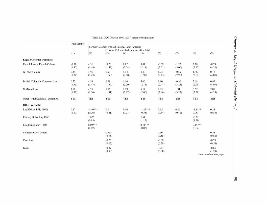
Chapter

3:LegalOrigin

orC

olonialHistory?

90

Table 3.3: GDP Growth 1960–2007, saturated regressions

Full SampleFormer Colonies without Europe, Latin America

Former Colonies Independent after 1960(1) (2) (3) (4) (5) (6) (7) (8) (9)

LegalXColonial Dummies

French Law X French Colony -0.31 4.31 -0.20 0.02 5.01 -0.39 -1.23 2.78 -0.78(1.30) (1.49) (1.57) (2.04) (2.14) (2.51) (3.06) (2.97) (4.20)

X Other Colony 0.49 3.95 0.93 1.14 4.40 1.23 -0.59 1.36 0.12(1.34) (1.43) (1.58) (2.00) (1.99) (2.43) (2.98) (2.82) (4.01)

British Colony X Common Law 0.72 4.53 0.98 1.16 5.00 1.10 -0.36 2.68 0.92(1.36) (1.47) (1.50) (2.20) (2.15) (2.47) (3.25) (2.98) (4.07)

X Mixed Law 1.80 4.75 1.86 2.29 5.17 2.03 1.31 3.52 2.08(1.37) (1.36) (1.51) (2.17) (2.00) (2.46) (3.22) (2.79) (4.23)

Other (legalXcolonial) dummies YES YES YES YES YES YES YES YES YES

Other Variables

Ln(GDP pc PPP, 1960) 0.17 -1.10*** 0.14 0.10 -1.29*** 0.15 0.26 -1.11** 0.23(0.17) (0.26) (0.21) (0.27) (0.38) (0.34) (0.42) (0.51) (0.56)

Primary Schooling 1960 1.62* 1.61 -0.21(0.85) (1.12) (1.30)

Life Expectancy 1960 0.09*** 0.11*** 0.15***(0.02) (0.03) (0.04)

Supreme Court Tenure 0.73* 0.66 0.38(0.38) (0.55) (0.88)

Case Law -0.26 -0.39 -0.75(0.25) (0.38) (0.56)

Juries -0.37 -0.47 -0.65(0.50) (0.88) (1.28)


Chapter

3:LegalOrigin

orC

olonialHistory?

91

Table 3.3: GDP Growth 1960–2007, saturated regressions



N 110 97 94 66 58 53 45 38 33R2 0.71 0.82 0.72 0.64 0.77 0.65 0.50 0.69 0.47

Combinations of LegalXColonialCoefficientsFrenchXFrench – FrenchXOther -0.80* 0.35 -1.13** -1.12* 0.61 -1.62* -0.65 1.42* -0.91

(0.41) (0.36) (0.49) (0.64) (0.61) (0.84) (0.84) (0.73) (1.31)

CommonXBritish – FrenchXOther 0.23 0.58* 0.046 0.017 0.61 -0.13 0.22 1.32* 0.80(0.41) (0.33) (0.57) (0.66) (0.58) (1.00) (0.90) (0.76) (1.48)

CommonXBritish –MixedXBritish -1.08* -0.22 -0.88 -1.13 -0.17 -0.93 -1.68* -0.84 -1.16(0.61) (0.53) (0.69) (0.69) (0.64) (0.82) (0.90) (0.80) (1.30)

p-values fromWald Tests of Joint HypothesesAll LegalXColonial Dummies 0.00 0.29 0.01 0.01 0.47 0.02 0.15 0.20 0.18Additional Controls 0.00 0.26 0.00 0.50 0.00 0.60

The regressions are estimated without a constant. OLS standard errors in parentheses. ∗ ∗ ∗p < .01, ∗ ∗ p < .05, ∗p < .10 (we do not attach asterisks to the estimates for theLegalXColonial dummies; these estimates only represent group-specific constants).

Data sources: GDP growth: Heston et al. (2009); colonizer, legal origin, supreme court tenure, case law, and juries: authors’ coding; primary schooling (gross primary enrollmentratio) and life expectancy (at birth): Barro & Lee (1994).

Chapter

3:LegalOrigin

orC

olonialHistory?

92

Table 3.4: GDP Growth 1960-2007, separate legal and colonial dummy sets



Origin of LawCommon -0.97 -0.21 -0.54 -1.18 0.15 -0.94 0.11 -0.84 -1.16

(0.79) (0.63) (0.97) (1.50) (1.28) (1.74) (1.44) (0.80) (1.30)

Mixed -0.03 -0.09 0.29 -0.23 0.19 -0.016 1.48(0.72) (0.57) (0.79) (1.34) (1.10) (1.48) (1.44)

German Civil 1.45* 0.43 1.62* 3.41* 2.35 4.00(0.83) (0.70) (0.89) (2.03) (1.79) (2.60)

Scandinavian Civil -0.046 -0.44 0.63(0.91) (0.75) (1.04)

ColonizerBritain 2.05** 0.42 1.83* 2.39 -0.10 2.43 0.90 0.74 2.86**

(0.84) (0.70) (1.02) (1.48) (1.31) (1.80) (1.37) (0.91) (1.26)

French Civil Law Country 0.81* -0.36 1.16** 1.11* -0.61 1.62* 0.62 -1.42* 0.91Other than France (0.41) (0.36) (0.49) (0.64) (0.61) (0.84) (0.84) (0.73) (1.31)

Other 1.87** 0.92 2.07* 1.34 -0.37 1.04 1.38(0.87) (0.79) (1.06) (1.69) (1.57) (2.34) (1.66)

None 1.40** 0.47 1.52**(0.64) (0.51) (0.69)

Other variablesLn(GDP pc PPP, 1960) 0.10 -1.22*** 0.11 0.06 -1.3*** 0.15 0.16 -1.11**

(0.16) (0.25) (0.20) (0.27) (0.38) (0.34) (0.41) (0.51)

Primary Schooling 1960 1.69** 1.53 -0.21(0.83) (1.11) (1.30)

Life Expectancy 1960 0.10*** 0.12*** 0.15***(0.02) (0.03) (0.05)


Chapter

3:LegalOrigin

orC

olonialHistory?

93

Table 3.4: GDP Growth 1960-2007, separate legal and colonial dummy sets



Supreme Court Tenure 0.68* 0.66 0.38(0.38) (0.55) (0.88)

Case Law -0.33 -0.39 -0.75(0.24) (0.38) (0.56)

Juries -0.40 -0.47 -0.65(0.49) (0.88) (1.28)

Constant 0.23 4.95*** 0.03 0.33 5.14** -0.39 -0.48 2.78 -0.78(1.27) (1.43) (1.54) (2.00) (2.13) (2.51) (2.97) (2.97) (4.20)

R2 0.23 0.53 0.27 0.27 0.53 0.32 0.18 0.54 0.24N 110 97 94 66 58 53 45 38 33

p-values fromWald Tests of Joint HypothesesLegal origin dummies 0.07 0.83 0.24 0.04 0.47 0.20 0.24 0.30 0.38Colonial dummies 0.11 0.35 0.10 0.21 0.72 0.23 0.62 0.11 0.44Legal and colonial dummies 0.00 0.26 0.00 0.01 0.43 0.02 0.13 0.20 0.18Common=Mixed 0.08 0.80 0.20 0.15 0.95 0.26 0.11 0.30 0.38Additional Controls 0.00 0.26 0.00 0.50 0.00 0.60

OLS standard errors in parentheses. ∗ ∗ ∗p < .01, ∗ ∗ p < .05, ∗p < .10

Data sources: GDP growth: Heston et al. (2009); colonizer, legal origin, supreme court tenure, case law, and juries: authors’ coding; primary schooling (gross primary enrollmentratio) and life expectancy (at birth): Barro & Lee (1994).


As with raw growth rates, when we control for initial GDP per capita there are substan-

tial differences between the different legal/colonial groups. As before, however, broader

colonial history rather than legal origin correlates with growth differences. As shown in

models 1, 4, and 7 of table 3.3, and as in table 3.2, for all the samples, French civil law

countries colonized by countries other than France did economically and statistically signif-

icantly better than former French colonies, and in fact did approximately as well as former

British colonies with common law legal systems. Also as before, former British colonies

with mixed legal systems did even better than former British colonies with pure common

law systems. We obtain similar results with the competing dummy sets in models 1, 4,

and 7 of table 3.4. Controlling for the colonizer, common law jurisdictions are statistically

indistinguishable from civil law jurisdictions; in fact, the point estimate suggests that com-

mon law is associated with lower growth, and common law jurisdictions grew statistically

significantly less than German civil law jurisdictions and mixed jurisdictions (in the full

sample). By contrast, the British colony coefficient is economically significantly positive,

and statistically significantly so in the full sample, implying that former British colonies

grew on average approximately 2% faster per year than former French colonies. Moreover,

former colonies of French civil law countries other than France also grew approximately

1% per year faster than French colonies; this difference is statistically significant except in

the small sample of former colonies independent after 1960 (model 7).

Further confirmation of the importance of colonial rather than legal origins comes

from the additional control variables that we introduce in the other regressions of ta-

bles 3.3 and 3.4. Our proxies for broader colonial policy - initial schooling and life ex-

pectancy - absorb most of the effect of the colonial dummies, and are at least jointly highly

significant, both statistically and economically. The point estimates in models 2 and 5 of

table 3.3 suggest that a one-standard deviation increase in initial schooling and life ex-

pectancy is associated with approximately 1.75% higher annual growth over the period

1960-2007. We showed in table 3.1 above that former British colonies had significantly

higher initial education and life expectancy around 1960. Together, these estimates pro-

vide reason to believe that the colonizing powers had an important differential effect on

post-colonial development through their non-legal policies.

By contrast, we find no evidence that legal institutions imposed by the colonial powers


had any effect on subsequent growth. The estimates for juries, case law, and supreme court

tenure are neither individually nor collectively significant, with the exception of supreme

court tenure in model 3 of table 3.3. Moreover, two of the three coefficients -case law and

juries - point in the "wrong" direction, i.e., they appear to be associated with lower growth,

the opposite of what the legal origins hypothesis would suggest (cf. section 2.2.1 above).

3.4 Other Dependent Variables: Financial Markets, Un-employment, and Institutions

We now perform identical tests for other dependent variables. As we will see, the

picture that emerges here is much less clear than for growth, and we have verified that

this is not a consequence of differing samples or different time periods.21 We defer the

discussion of these discrepancies to section 5 below.

While there are potentially hundreds of dependent variables to look at, we focus on the

key areas of the legal origins literature, as summarized in La Porta et al. (2008, Tables 1-3,

panels B): equity markets, debt markets, employment, corruption, and the functioning of

the judiciary. For each of those broad areas, we retain from La Porta et al. (2008, Tables

1-3, panels B) the dependent variable with the greatest country coverage: stock market

capitalization to GDP, private credit to GDP, unemployment, corruption, and the duration

of court proceedings to enforce a debt. Unlike La Porta et al. (2008), however, we are

not constrained by the use of time-variant legal variables to work with data for a particular

time period, and we therefore use the most recent available data with the greatest country

coverage. With one exception, we average the data over a ten-year period to filter out

cyclical noise and to maximize sample size.22

In particular, we average 1998-2007 data on stock market capitalization over GDP,

private credit over GDP, and unemployment from the World Bank’s World Development

Indicators (WDI), and meta-data on corruption (rescaled so that higher numbers indicate

21Running our growth regressions for the period 1998-2007 yields few significant results, presumablybecause of the relatively short time window, but the coefficient estimates are similar to those of our baselinegrowth regressions.

22In averaging the data, we average over all available years for the particular country in the relevant timeperiod, instead of dropping countries with missing data for some of those years.


more corruption) from the World Bank’s World Governance Indicators. In addition, we use

the World Bank’s latest Doing Business Report (World Bank 2008) data on the duration of

enforcing a simple business debt in the year 2006.23 As La Porta et al. (2008) do, we control

in all regressions for the natural logarithm of GDP per capita from WDI, PPP-adjusted and

averaged over 1998-2007. The other independent variables are the same as in the growth

regressions.

While our regression specifications and tests are otherwise identical to those we used

for growth above, we condense the presentation because we now have five times as many

regressions. We report for each regression only the coefficients and test statistics that are di-

rectly relevant for distinguishing legal and other colonial origins in these data, as explained

in section 2 above and applied with respect to growth in section 3. We also report only

results for the conceptually most convincing sample, namely former colonies outside of

Europe and Latin America, for which legal origin is clearly exogenous. We have verified,

however, that results for the full sample are similar.

In addition to single-equation test statistics, we also show p-values from corresponding

joint cross-equation Wald tests using the covariance matrix estimate from unweighted sys-

tem OLS.24 Since we have considerably fewer observations for equity market capitalization

than for our other dependent variables, we also show cross-equation tests for the other four

dependent variables.

23The latest Doing Business data replace those of Djankov et al. (2003) and the World Bank’s first DoingBusiness Report (World Bank 2004); as documented in Spamann (2010), they deviate substantially from theearlier, less sophisticated data.

24Some of these p-values need to be interpreted with caution because they do not account for the directionin which an estimate deviates from the null-hypothesis. For example, if common law countries perform worsethan French civil law countries in one equation and better in another, these deviations from a null-hypothesisof no differences do not cancel out but rather add up in the cross-equation test.

Chapter

3:LegalOrigin

orC

olonialHistory?

97

Table 3.5: Other Dependent Variables, Saturated Regressions

Marketcap/GDP

Credit/GDP Corruption Unemployment Court Duration Joint p-values for equations

(1) (2) (3) (4) (5) (1)-(5) (2)-(4)

Panel A – No Additional Control VariablesN 50 103 73 105 100 43 70R2 0.51 0.56 0.13 0.61 0.11

FrenchXFrench – FrenchXOther 14.35 2.79 -3.78 -0.22 -72.60 0.18 0.02(32.80) (8.68) (2.83) (0.16) (96.35)

CommonXBritish – FrenchXOther 46.49** 19.62** -3.02 -0.54*** -91.60 0.00 0.00(22.26) (8.25) (2.45) (0.15) (92.34)

CommonXBritish – MixedXBritish 33.94 -10.29 -5.78** 0.07 -205.93 0.01 0.03(23.43) (10.76) (2.55) (0.20) (128.73)

p-Values from Wald TestsAll LegalXColonial Dummies 0.47 0.24 0.46 0.09 0.54 0.03 0.19

Panel B – Proxies for Colonial Policy (Education, Life Expectancy)N 36 62 47 62 61 33 46R2 0.58 0.66 0.37 0.75 0.18

FrenchXFrench – FrenchXOther 10.81 -9.86 0.82 -0.03 -57.66 0.55 0.28(60.79) (14.67) (4.11) (0.23) (134.26)

CommonXBritish – FrenchXOther 71.49 0.85 -0.99 -0.11 -83.25 0.32 0.12(48.04) (13.73) (3.64) (0.21) (126.04)

CommonXBritish –MixedXBritish 41.06 -11.28 -8.72*** 0.11 -219.81 0.01 0.00(28.90) (14.65) (2.78) (0.23) (142.44)

p-Values from Wald TestsAll LegalXColonial Dummies 0.37 0.98 0.09 0.95 0.70 0.00 0.00Colonial Policy Proxies 0.07 0.27 0.06 0.02 0.49 0.13 0.21


Chapter

3:LegalOrigin

orC

olonialHistory?

98

Table 3.5: Other Dependent Variables, Saturated Regressions

Marketcap/GDP

Credit/GDP Corruption Unemployment Court Duration Joint p-values for equations

(1) (2) (3) (4) (5) (1)-(5) (2)-(4)

Panel C – Proxies for Legal Families (Juries, Case Law, Supreme Court Tenure)N 37 64 48 64 60 32 45R2 0.59 0.67 0.21 0.70 0.23

FrenchXFrench – FrenchXOther 4.89 12.23 -2.27 -0.51** -74.70 0.65 0.18(31.53) (12.33) (3.86) (0.23) (116.56)

CommonXBritish – FrenchXOther 5.65 1.82 -2.25 -0.59** -58.37 0.15 0.05(29.87) (15.41) (4.31) (0.29) (144.77)

CommonXBritish –MixedXBritish 16.24 -22.85* -6.08** 0.10 -221.77* 0.04 0.01(18.63) (12.81) (2.94) (0.24) (126.72)

p-Values from Wald TestsAll LegalXColonial Dummies 0.78 0.78 0.64 0.50 0.30 0.43 0.00Legal Family Proxies 0.51 0.01 0.49 0.25 0.51 0.62 0.16

This table only shows linear combinations of coefficients and corresponding OLS standard errors (in parentheses), as well

as p-values for joint hypotheses within and across equations. The full regression specifications of panels A-C are identical

to those of equations (4)-(6), respectively, of table 3.3, with the exception of the dependent variables and the control for

ln(GDP per capita) (1998-2007 from the World Development Indicators, instead of 1960 from Heston et al. 2009). The first

four dependent variables are averaged over the years 1998-2007 and come from the World Bank’s World Development

Indicators (stock market capitalization over GDP, private credit over GDP, and unemployment) and World Governance

Indicators (corruption, rescaled so that higher numbers indicate more corruption); the fifth dependent variable (duration

of enforcing a simple business debt in the year 2006) is from World Bank (2008). ∗ ∗ ∗p < .01, ∗ ∗ p < .05, ∗p < .10


Table 3.5 shows results from regressions with dummies for the various combinations of

legal and colonial origin, i.e., the equivalent of table 3.3, models (4)-(6). Panel A shows

the regressions controlling only for contemporaneous GDP per capita and legal/colonial

origin. The picture is almost the opposite of what we find for growth. Among French le-

gal origin countries, former French colonies now perform better than other colonies with

French civil law on all five dimensions. Although the individual differences are not statisti-

cally significant, collectively they are, if market capitalization is omitted from the test. The

exclusion of market capitalization is important, because it doubles the sample size. Also

unlike for growth, non-French colonies with French civil law perform much worse than

former British colonies with common law. Among former British colonies, the mixed ju-

risdictions perform better than pure common law countries in some areas but not in others,

and only one of those differences is individually statistically significant (the joint p-value

is 0.01, but it confounds positive and negative deviations).

We get results more consistent with our growth results in panel B, which shows results

from regressions with controls for non-legal colonial policy, namely education and life

expectancy in 1960 (see section 2.2.2 above). These proxies absorb most of the differences

between the various legal/colonial groups, particularly the differences between French and

other former colonies with French civil law; and the differences in average private credit,

corruption, and unemployment between former British, common law colonies and former

non-French, French civil law colonies. By contrast, the differences between common law

and mixed former British colonies are unaffected. The colonial proxies themselves are not

statistically significant except in the unemployment and corruption equations, but this may

be due to the fact that the particular proxies we use are not well-matched to the dependent

variables (see section 2.2.2 above).

The results from regressions with proxies for common/civil law differences, namely

juries, case law, and supreme court tenure (see section 2.2.1 above), are consistent with our

growth results in so far as these legal proxies are jointly insignificant across all equations

and in every single equation except the credit market regression.

We have also run the table 3.5 regressions with competing sets of legal and colonial

origin dummies, i.e., the equivalent of the growth regressions in table 3.4 (models 4-6).

The unreported results confirm those of table 3.5. In particular, across all five dimensions,


common law is associated with favorable outcomes, while British colonial influence is

associated with unfavorable outcomes. These estimates, however, are statistically insignif-

icant except for market capitalization.

To sum up, we find, for the other dependent variables, mixed jurisdictions perform

on the whole as well as common law jurisdictions, while the legal origins theory would

predict that they do worse. At the same time, unlike for growth and contrary to the colonial

history hypothesis, former French colonies do better for the other dependent variables than

colonies of French civil law countries other than France. Neither proxies for colonial policy

(education and life expectancy in 1960) nor for legal institutions (juries, case law, supreme

court tenure) seem to matter in these regressions.

3.5 Discussion

In order to interpret our results, we first need to reconcile our results for growth with

those for other dependent variables. While the former strongly suggest that colonial history

rather than legal origin explains performance differences, the latter are more ambiguous

and, in part, point in the opposite direction. As already mentioned, we have verified that

the differences are only partially explained by differing time periods and samples.

The discrepancy is puzzling because most economists believe that these other depen-

dent variables - capital markets, labor force utilization, and institutions - are important

for economic growth (see, e.g., for capital markets Geert Bekaert, Campbell Harvey, and

Christian Lundblad 2005), and also that there is a feedback effect from economic develop-

ment to these other variables. We would therefore expect these estimates to go in the same

direction, and the discrepancy, if it is one, is more than the usual statistical outlier that we

would expect when conducting multiple independent tests. Of course, there is no puzzle

to explain if the results for the other dependent variables are simply non-results, i.e., noise.

This is plausible because few if any of the results for the other dependent variables were

statistically significant by conventional standards.

To be sure, the "noise explanation" is ultimately not satisfactory, and calls for additional

work. Another possibility is that common law countries may have negative features which

offset the advantages identified by La Porta et al. (2008) and others. Chapter 2 shows that


common law countries have higher incarceration rates and more crime. Similarly, David

Cutler, Edward Glaeser and Jesse Shapiro (2003) find that common law countries have

higher obesity rates. These and other yet undiscovered negative characteristics of common

law countries may counteract the positive characteristics more prominent in the literature.

For the time being, we read the evidence that we find here in conjunction with other

papers that shed light on the respective relevance of colonial history and legal origins.

While we are the first to address the former as an alternative to legal origins, others have

questioned the theory behind the legal origins explanation from different angles. Mark

Roe (2006) points out that much of the evidence of the legal origins literature is drawn

from highly regulatory areas of law, such as securities or conscription, which have no

obvious link to what are traditionally perceived to be the main differences between common

and civil law, such as the recognition of case law and various aspects of civil procedure.

Moreover, Spamann (2010) shows that the best available data on civil procedure (World

Bank 2008) exhibit no measurable differences between common and civil law countries.

Together with the results of this paper, this suggests that non-legal colonial explanations

deserve to be taken seriously as explanations for the observed cross-country differences

between "common law" and "civil law" countries.

3.6 Conclusion

In this paper, we argue that colonial history is a plausible alternative to purely legal

explanations for the empirical patterns documented in the legal origins literature. The

colonial powers not only imposed their legal system but also had other profound influences

on their colonies, including educational policy, health policy, and local administration and

self-government. Empirically, we can show that the identity of the colonizer is indeed a

better predictor of post-colonial growth rates than legal origin, and this is bolstered by our

finding that proxies for broader colonial policy, but not proxies for legal origin, can explain

much of the growth differential between the colonial groups. For other dependent variables,

the results are mixed, pointing to the need for further research.

References

Acemoglu, Daron and Simon Johnson, “Disease and Development: The Effect of Life

Expectancy on Economic Growth,” Journal of Political Economy, 2007, 115, 925–85.

, , and James A. Robinson, “Colonial Origins of Comparative Development: An

Empirical Investigation,” American Economic Review, 2001, 91, 1369–1401.

Albouy, David, “The Colonial Origins of Comparative Development: An Empirical

Investigation: Comment,” American Economic Review. Forthcoming.

Alesina, Alberto, Arnaud Devleeschauwer, William Easterly, Sergio Kurlat, and

Romain Wacziarg, “Fractionalization,” Journal of Economic Growth, 2003, 8,

155–194.

Anckar, Carsten, Determinants of the Death Penalty—A comparative study of the world,

London and New York: Routledge, 2006.

Avellaneda, Marco and Rama Cont, Transparency in Credit Default Swap Markets,

Paris: Finance Concepts, 2010.

Barro, Robert and Jong-Wha Lee, “Data Set for a Panel of 138 Countries,” 1994.

Available at http://www.columbia.edu/~xs23/data/barrlee.htm

(accessed August 2008).

Beck, Thorsten, Aslı Demirgüç-Kunt, and Ross Levine, “Law and Finance: Why Does

Legal Origin Matter?,” Journal of Comparative Economics, 2003, 31, 653–75.

Bedendo, Mascia, Lara Cathcart, and Lina El-Jahel, “In- and Out-of-Court Debt

Restructuring in the Presence of Credit Default Swaps,” 2012. Working paper, Bocconi

102

References 103

University and Imperial College, available at

http://ssrn.com/abstract=1666101 (visited March 15, 2012).

Bekaert, Geert, Campbell R. Harvey, and Christian Lundblad, “Does Financial

Liberalization Spur Growth?,” Journal of Financial Economics, 2005, 77, 3–55.

Bertocchi, Graziella and Fabio Canova, “Did colonization matter for growth? An

empirical exploration into the historical causes of Africa’s underdevelopment,”

European Economic Review, 2002, 46, 1851–71.

Blumstein, Alfred, Michael Tonry, and Asheley van Ness, “Cross-National Measures of

Punitiveness,” in Michael Tonry and David P. Farrington, eds., Crime and Punishment

in Western Countries, 1980–1999, Crime and Justice: A Review of Research 33,

Chicago: University of Chicago Press, 2005, pp. 347–376.

Bolton, Patrick and Martin Oehmke, “Credit Default Swaps and the Empty Creditor

Problem,” Review of Financial Studies, 2011, 24, 2617–2655.

Borjas, George J. and Glenn T. Sueyoshi, “A two-stage estimator for probit models with

structural group effects,” Journal of Econometrics, 1994, 64, 165–182.

Brav, Alon and Richmond Mathews, “Empty Voting and the Efficiency of Corporate

Governance,” Journal of Financial Economics, 2011, 99, 289–307.

Burdett, Kenneth, Ricardo Lagos, and Randall Wright, “Crime, Inequality, and

Unemployment,” American Economic Review, 2003, 93, 1764–1777.

Campbell, Christian (ed.), Legal Aspects of Doing Business in the Middle East,

Netherlands: Kluwer Law International, 2006.

Campello, Murillo and Rafael Matta, “Credit Default Swaps, Firm Financing and the

Economy,” 2012. Working paper, Cornell University and University of Illinois,

available at http://ssrn.com/abstract=1770066 (visited March 15, 2012).

Cavadino, Michael and James Dignan, “Penal Policy and Political Economy,”

Criminology & Criminal Justice, 2006, 6, 435–456.

References 104

and , Penal Systems: A Comparative Approach, London, Thousand Oaks, and New

Delhi: SAGE, 2006.

Chen, Kathryn, Michael Fleming, John Jackson, Ada Li, and Asani Sarkar, “An

Analysis of CDS Transactions: Implications for Public Reporting,” Technical Report

517, Federal Reserve Bank of New York September 2011.

Christoffersen, Susan, Christopher Geczy, David Musto, and Adam Reed, “Vote

Trading and Information Aggregation,” Journal of Finance, 2007, 62, 2897–2939.

CIA, “World Factbook 2008,” 2008. At

www.cia.gov/library/publications/the-world-factbook, visited

6/01/2008.

Clear, Todd R., “The Effects of High Imprisonment Rates on Communities,” Crime and

Justice: A Review of Research, 2008, 37, 97–132.

Cutler, David, Edward Glaeser, and Jesse Shapiro, “Why Have Americans Become

More Obese?,” Journal of Economic Perspectives, 2003, 17 (3), 93–118.

Da, Zhi and Pengjie Gao, “Clientele Change, Persistent Liquidity Shock, and Bond

Return Reversals After Rating Downgrades,” 2009. Working paper, University of Notre

Dame, available at http://nd.edu/~zda/Bond.pdf (visited March 15, 2012).

David, Réné et al., eds., International Encyclopedia of International Law, Vol. 1:

National Reports, Tubingen: Mohr Siebeck, 1973–88.

Deininger, Klaus and Lyn Squire, “A New Data Set Measuring Income Inequality,”

World Bank Economic Review, 1996, 10, 565–591.

Djankov, Simeon, Edward Glaeser, Rafael La Porta, Florencio Lopez de Silanes, and

Andrei Shleifer, “The New Comparative Economics,” Journal of Comparative

Economics, 2003, 31, 595–619.

, Rafael La Porta, Florencio Lopez de Silanes, and Andrei Shleifer, “The law and

economics of self-dealing,” Journal of Financial Economics, 88, 430–465.

References 105

Downes, David and Kirstine Hansen, “Welfare and Punishment in Comparative

Perspective,” in Sarah Armstrong and Lesley McAra, eds., Perspectives on Punishment,

Oxford: Oxford University Press, 2006, pp. 133–154.

and , “Welfare and punishment: The relationship between welfare spending and

imprisonment, Crime and Society Foundation briefing 2,” Technical Report, Crime and

Society Foundation, London November 2006.

Elkins, Zachary, Tom Ginsburg, and James Melton, “Characteristics of National

Constitutions Dataset v. 1.0,” 2010. Available at

http://www.comparativeconstitutionsproject.org/data.htm.

Esping-Andersen, Gosta, The Three Worlds of Welfare Capitalism, Princeton: Princeton

University Press, 1990.

Fajnzylber, Pablo, Daniel Lederman, and Norman Loayza, “Inequality and Violent

Crime,” Journal of Law and Economics, 2002, 45, 1–40.

Fearon, James D., “Ethnic and Cultural Diversity by Country,” Journal of Economic

Growth, 2003, 8, 195–222.

Frase, Richard S., “Sentencing and Comparative Law Theory,” in John Jackson, Máximo

Langer, and Peter Tillers, eds., Crime, Procedure and Evidence in a Comparative and

International Context, Oxford and Portland, Oregon: Hart Publishing, 2008,

pp. 351–369.

Gibson, John and Bonggeun Kim, “The effect of reporting errors on the cross-country

relationship between inequality and crime,” Journal of Development Economics, 2008,

87, 247–254.

Glaeser, Edward L. and Andrei Shleifer, “Legal Origins,” Quarterly Journal of

Economics, 2002, 117, 1193–1229.

Greenberg, David F. and Valerie West, “Siting the Death Penalty Internationally,” Law

& Social Inquiry, 2008, 33, 295–343.

References 106

Grier, Robin M., “Colonial legacies and economic growth,” Public Choice, 1999, 98,

317–35.

Gwartney, James and Robert Lawson, Economic Freedom of the World: 2007 Annual

Report, Vancouver, B.C.: Fraser Institute, 2007. With Russell S. Sobel and Peter T.

Leeson. Data retrieved from www.freetheworld.com.

Hall, Peter A. and David Soskice, “An Introduction to Varieties of Capitalism,” in

Peter A. Hall and David Soskice, eds., Varieties of Capitalism: the institutional

foundations of comparative advantage, Oxford and New York: Oxford University

Press, 2001, pp. 1–68.

Hayek, Friedrich A., The Constitution of Liberty, Chicago: University of Chicago Press,

1960.

, Law, legislation, and liberty: a new statement of the liberal principles of justice and

political economy, Vol. 1 of Rules and Order, Chicago: University of Chicago Press,

1973.

Heston, Alan, Robert Summers, and Bettina Aten, “Penn World Table Version 6.3,”

August 2009. Center for International Comparisons of Production, Income and Prices

at the University of Pennsylvania.

Hirschi, Travis and Michael Gottfredson, “Age and the Explanation of Crime,”

American Journal of Sociology, 1983, 89, 552–584.

Hu, Henry and Bernard Black, “The New Vote Buying: Empty Voting and Hidden

(Morphable) Ownership,” Southern California Law Review, 2006, 79, 811–908.

and , “Hedge Funds, Insiders, and the Decoupling of Economic and Voting

Ownership: Empty Voting and Hidden (Morphable) Ownership,” Journal of Corporate

Finance, 2007, 13, 343–367.

and , “Debt, Equity and Hybrid Decoupling: Governance and Systemic Risk

Implications,” European Journal of Financial Management, 2008, 14, 663–709.

References 107

Hunt, Jennifer, “Do teen births keep American crime high?,” Journal of Law and

Economics, 2006, 49, 533–566.

International Center for Prison Studies, “World Prison Brief,” 2008. At http://

www.kcl.ac.uk/depsta/law/research/icps/worldbrief/

index.php?search=All, visited 4/24/08.

INTERPOL, “International Crime Statistics for 1999,” 1999. Saint Cloud: INTERPOL.

Kim, Kensie, “Mixed Systems in Legal Origins Analysis,” Southern California Law

Review, 2010, 83, 693–730.

Klerman, Daniel, Paul Mahoney, Holger Spamann, and Mark Weinstein, “Legal

Origin or Colonial History?,” Journal of Legal Analysis, 2011, 3 (2).

Kyle, Albert, “A Theory of Futures Market Manipulations,” in Ronald Anderson, ed., The

Industrial Organization of Futures Markets, Lexington, MA: Lexington Books, 1984,

pp. 141–173.

, “Continuous Auctions and Insider Trading,” Econometrica, 1985, 53, 1315–1335.

and Jean-Luc Vila, “Noise Trading and Takeovers,” RAND Journal of Economics,

1991, 22, 54–71.

La Porta, Rafael, Florencio Lopez de Silanes, and Andrei Shleifer, “What works in

securities laws?,” Journal of Finance, 2006, 61, 1–32.

, , and , “The Economic Consequences of Legal Origins,” Journal of Economic

Literature, 2008, 46, 285–332.

, , , and Robert Vishny, “The Quality of Government,” Journal of Law,

Economics, and Organization, 1999, 15, 222–279.

, , Cristian Pop-Eleches, and Andrei Shleifer, “Judicial Checks and Balances,”

Journal of Political Economy, 2004, 112, 445–470.

References 108

Lappi-Seppälä, Tapio, “Trust, Welfare, and Political Culture: Explaining Differences in

National Penal Policies,” Crime and Justice: A Review of Research, 2008, 37, 313–387.

Levine, Ross and David Renelt, “A Sensitivity Analysis of Cross-Country Growth

Regressions,” American Economic Review, 1992, 82, 942–63.

Levitt, Steven D., “Understanding Why Crime Fell in the 1990s: Four Factors that

Explain the Decline and Six that Do Not,” Journal of Economic Perspectives, 2004, 18,

163–190.

and Thomas J. Miles, “Empirical Study of Criminal Punishment,” in A. Mitchell

Polinsky and Steven Shavell, eds., Handbook of Law and Economics, Vol. 1,

Amsterdam: North-Holland, 2007, pp. 455–495.

Licht, Amir N., Chanan Goldschmidt, and Shalom H. Schwartz, “Culture Rules: The

foundations of the rule of law and other norms of governance,” Journal of Comparative

Economics, 2007, 35, 659–688.

Lijphart, Arend, Patterns of Democracy: Government Forms and Performance in

Thirty-Six Countries, New Haven and London: Yale University Press, 1999.

Lin, Ming-Jen, “Does democracy increase crime? The evidence from international data,”

Journal of Comparative Economics, 2007, 35, 467–483.

Liptak, Adam, “Inmate Count in U.S. Dwarfs Other Nations’,” New York Times, April 23,

2008.

Listokin, Yair, “Does more crime mean more prisoners?,” Journal of Law and

Economics, 2003, 46, 181–206.

Lynch, James P., “Problems and Promise of Victimization Surveys for Cross-National

Research,” in Michael Tonry, ed., Crime and Justice: A Review of Research 34,

Chicago: University of Chicago Press, 2006, pp. 229–287.

Mahoney, Paul G., “The Common Law and Economic Growth: Hayek Might be Right,”

Journal of Legal Studies, 2001, 30, 503–25.

References 109

Martin, Shaun and Frank Partnoy, “Encumbered Shares,” University of Illinois Law

Review, 2005, 2005, 775–813.

McCleary, Rachel M. and Robert J. Barro, “Religion and Economy,” Journal of

Economic Perspectives, 2006, 20 (2), 49–72.

Merryman, John Henry, “The French Deviation,” American Journal of Comparative

Law, 1996, 44, 109–19.

Messner, Steven F., Lawrence E. Raffalovich, and Peter Shrock, “Reassessing the

Cross-National Relationship between Income Inequality and Homicide Rates:

Implications of Data Quality Control in the Measurement of Income Distribution,”

Journal of Quantitative Criminology, 2002, 18, 377–395.

Mukherjee, Satyanshu and Philip Reichel, “Bringing to Justice,” in Graeme Newman,

ed., Global Report on Crime and Justice, New York and Oxford: Oxford University

Press, 1999, pp. 65–88.

Murray, Joseph and David P. Farrington, “The Effects of Parental Imprisonment on

Children,” Crime and Justice: A Review of Research, 2008, 37, 133–206.

Neapolitan, Jerome L., Cross-National Crime: A Research Review and Sourcebook,

Westport, CT and London: Greenwood Press, 1997.

, “An Examination of Cross-National Variation in Punitiveness,” International Journal

of Offender Therapy and Comparative Criminology, 2001, 45, 691–710.

Newman, Graeme and Gregory J. Howard, “Introduction: Data sources and their use,”

in Graeme Newman, ed., Global Report on Crime and Justice, New York and Oxford:

Oxford University Press, 1999, pp. 1–23.

Pagano, Marco and Paolo F. Volpin, “The Political Economy of Corporate Governance,”

American Economic Review, 2005, 95, 1005–1030.

Pease, Ken, “Cross-National Imprisonment Rates: Limitations of Method and Possible

Conclusions,” British Journal of Criminology, 1994, 34 (special issue), 116–130.

References 110

Peristiani, Stavros and Vanessa Savino, “Are Credit Default Swaps Associated with

Higher Corporate Defaults?,” Technical Report 494, Federal Reserve Bank of New

York May 2011.

PEW Center on the States, “One in 31: The Long Reach of American Corrections,”

Technical Report, Washington, DC March 2009.

Rajan, Raghuram G. and Luigi Zingales, “The Great Reversals: The Politics of

Financial Development in the Twentieth Century,” Journal of Financial Economics,

2003, 69, 5–50.

Reynolds, Thomas and Arturo Flores, “Foreign Law Guide: Current Sources of Codes

and Basic Legislation in Jurisdictions of the World,” 2008. At

www.foreignlawguide.com, visited 6/2/2008.

Roberts-Wray, Kenneth, Commonwealth and Colonial Law, New York: Frederick A.

Praeger, 1966.

Roe, Mark J., “Legal Origins, Politics, and Modern Stock Markets,” Harvard Law

Review, 2006, 120, 460–527.

and Jordan I. Siegel, “Finance and Politics: A Review Essay Based on Kenneth

Dam’s Analysis of Legal Traditions in The Law-Growth Nexus,” Journal of Economic

Literature, 2009, 47, 781–800.

Rostowski, Jacek and Bogdan Stacescu, “The Wig and the Pith Helmet—the Impact of

“Legal School” versus Colonial Institutions on Economic Performance (second

version),” Technical Report 2006. CEPR Studies & Analyses No. 300.

Ruddell, Rick, “Social Disruption, State Priorities, and Minority Threat,” Punishment &

Society, 2005, 7, 7–28.

Sala-i-Martin, Xavier, Gernot Doppelhofer, and Ronald I. Miller, “Determinants of

Long-Term Growth: A Bayesian Averaging of Classical Estimates (BACE) Approach,”

American Economic Review, 2004, 94, 813–35.

References 111

Sender, Henny, “Greenlight Capital founder calls for CDS ban,” Financial Times,

November 6, 2009.

Soares, Rodrigo R., “Development, crime, and punishment: accounting for the

international difference in crime rates,” Journal of Development Economics, 2004, 73,

155–184.

, “The welfare cost of violence across countries,” Journal of Health Economics, 2004,

25, 821–846.

Soros, George, “America must face up to the dangers of derivatives,” Financial Times,

April 22, 2010.

Soskice, David and Torben Iversen, “Inequality and Redistribution: A Unified Approach

to the Role of Economic and Political Institutions,” 2008. Mimeo, Oxford University

and Harvard University.

Spamann, Holger, “Contemporary Legal Transplants—Legal Families and the Diffusion

of (Corporate) Law,” Brigham Young University Law Review, 2009, 2009, 1813–77.

, “Legal Origins, Civil Procedure, and the Quality of Contract Enforcement,” Journal of

Institutional and Theoretical Economics, 2010, 166, 149–65.

Spelman, William, “Specifying the Relationship Between Crime and Prisons,” Journal of

Quantitative Criminology, 2008, 24, 149–178.

Steinhauer, Jennifer, “To Cut Costs, States Relax Prison Policies,” New York Times,

March 25, 2009.

Stulz, René, “Credit Default Swaps and the Credit Crisis,” Journal of Economic

Perspectives, 2010, 24 (1), 73–92.

Tonry, Michael, “Determinants of Penal Policies,” in Michael Tonry, ed., Crime,

Punishment, and Politics in Comparative Perspective, Chicago: University of Chicago

Press, 2007, pp. 1–48. Crime and Justice: A Review of Research 36.

References 112

and David P. Farrington, “Punishment and Crime across Space and Time,” in

Michael Tonry and David P. Farrington, eds., Crime and Punishment in Western

Countries, 1980–1999, Chicago: University of Chicago Press, 2005, pp. 1–39. Crime

and Justice: A Review of Research 33.

, , and Matthew Melewski, “The Malign Effect of Drug and Crime Control Policies

on Black Americans,” Crime and Justice: A Review of Research, 2008, 37, 1–44.

van Dijk, Jan, John van Kesteren, and Paul Smit, Criminal Victimization in

International Perspective: Key findings from the 2004-2005 ICVS and EU ICS, The

Hague: WODC, 2007.

van Kesteren, John, “Integrated Database from the International Crime Victim Surveys

(ICVS) 1989-2005, Data and Codebook,” 2007. Available at

http://easy.dans.knaw.nl., database ID P1749.

Vidmar, Neil, World Jury Systems, Oxford: Oxford University Press, 2000.

Voigt, Stefan, “The (Economic) Effects of Lay Participation in Courts—A Cross-Country

Analysis.” Forthcoming.

Whitman, James Q., Harsh Justice: Criminal Punishment and the Widening Divide

between America and Europe, Oxford and New York: Oxford University Press, 2003.

, “The Comparative Study of Criminal Punishment,” Annual Review of Law and Social

Science, 2005, 1, 17–34.

Wooldridge, Jeffrey M., “Cluster-Sample Methods in Applied Econometrics,” American

Economic Review (papers & proceedings), 93, 133–138.

World Bank, Doing Business in 2004: Understanding Regulation, Washington D.C.:

World Bank and Oxford University Press, 2004.

, Doing Business 2009, Washington D.C.: World Bank, 2008.

References 113

World Health Organization, “Mortality and Burden of Disease Estimates for WHO

Member States in 2004,” 2009. Available at http://www.who.int, visited

5/05/2009.

Young, Warren and Mark Brown, “Cross-National Comparisons of Imprisonment,” in

Michael Tonry, ed., Crime and Justice: A Review of Research, Vol. 17, Chicago:

University of Chicago Press, 1993, pp. 1–45.

Zachariadis, Konstantinos and Ioan Olaru, “The Impact of Security Trading on

Corporate Restructurings,” 2011. Working paper, London School of Economics,

available at http://ssrn.com/abstract=1652152 (visited March 15, 2012).

Zweigert, Konrad and Hein Kötz, Introduction to Comparative Law, 3rd ed.,

Oxford/New York: Clarendon Press/Oxford University Press, 1998. Trans. Tony Weir.

Documents

Essays in Applied Microeconomics - Harvard University