Embed Size (px)
Citation preview

Clemson UniversityTigerPrints
All Dissertations Dissertations
5-2014
ESSAYS ON ADAPTATION TO CLIMATECHANGEMargarita PortnykhClemson University, [email protected]
Follow this and additional works at: https://tigerprints.clemson.edu/all_dissertations
Part of the Economics Commons
This Dissertation is brought to you for free and open access by the Dissertations at TigerPrints. It has been accepted for inclusion in All Dissertations byan authorized administrator of TigerPrints. For more information, please contact [email protected].
Recommended CitationPortnykh, Margarita, "ESSAYS ON ADAPTATION TO CLIMATE CHANGE" (2014). All Dissertations. 1388.https://tigerprints.clemson.edu/all_dissertations/1388

ESSAYS ON ADAPTATION TO CLIMATE CHANGE
A Dissertation Presented to
the Graduate School of Clemson University
In Partial Fulfillment
of the Requirements for the Degree Doctor of Philosophy
Economics
by Margarita Portnykh
May 2014
Accepted by: Dr. Thomas Mroz, Committee Chair
Dr. William Dougan Dr. Curtis Simon Dr. Kevin Tsui

ii
ABSTRACT
Climate change represents a formidable challenge for mankind going forward. It is
important to understand its effects. In this thesis I study how people adopt to climate
change and argue that these responses could go a long way towards mitigating the effects
of climate change. I show that in some cases accounting for such adaptation could
completely reverse the negative effects of climate change.
In the first chapter of my thesis I consider the general impact of adaptation
without focusing on a particular adaptation mechanism studying mortality in Russia.
Using regional monthly mortality and daily temperature data, I estimate a flexible non-
parametric relation between weather and mortality. I find evidence that regions are better
adapted to temperature ranges they experience more frequently. In particular, damages
from the high heat are smaller in regions where the average summer temperature is higher
and damages from cold are lower in regions where winters are usually more severe. On
the basis of these estimates I propose a novel way to account for adaptation to climate
change without restricting attention to one particular channel. Namely, I assume that if
some currently cold region in the future will be exposed to the high heat on a regular
basis, then its (future) response will be similar to the present response of a warmer region
which currently is exposed to such heat on a regular basis. I illustrate my approach
constructing predictions for the impact of climate change on mortality using business-as-
usual temperature predictions from several climate change models. I find that the no-
adaptation specification predicts 0.7 percent increase in mortality by 2070-2099. When

iii
adaptation response is taken into account, however, I forecast a decrease in mortality by 1
percent by 2070-2099.
In the second chapter of my thesis I study migration as an adaptation mechanism
to climate change. I estimate a discrete location choice model, in which households
choose residence locations on the basis of potential earnings, moving costs, climate
amenities, and population density. I treat population density as endogenous using
geological structure as an instrument. This model allows me to estimate counterfactual
migratory responses and welfare changes resulting from non-marginal changes in
temperature, such as these predicted by most climate models. I also account for general
equilibrium effects on population densities arising from individual migration decisions. I
find that the costs of climate change are likely to be quite large. In the absence of
migration, American households would require their incomes to increase by 20-30
percent on average to attain their present day level of utility. The distribution of those
costs is uneven across geographical locations. Some areas in the South would require
more than 50 percent increases in terms of current incomes, while some northern
locations actually see benefits around 20 percent. Allowing for migratory responses
decrease those extremes considerably because of the resulting shifts in population
densities. For the hardest hit areas, migration would reduce the costs by more than 10
percent (4-5 percentage points). Areas benefiting the most from climate change without
migration would see their benefits reduced due to migratory inflows from other locations.

iv
DEDICATION
To my family for help and inspiration

v
ACKNOWLEDGMENTS
I would like to thank the members of my thesis committee: Thomas Mroz,
William Doungan, Curtis Simon, and Kevin Tsui for valuable advice, constructive
critique, and emotional support thourought different stages of my dissertation. I also
would like to extend my gratitude to Dan Benjamin who helped me to get started thinking
about environmental economics problems and climate change in particular. I am also
grateful for members of Labor Economics and Public Economics workshops for their
lively discussions and useful comments, which considerably enriched my analysis. I also
would like to thank Bobby McCormick, Olivier Deschenes, Michael Maloney, Matthew
Neidel, Randy Rucker, Walter Thurman, and Matthew Turner for their valuable
suggestions. I also would like to acknowledge intellectual support from the Property and
Environment Research Center in Bozeman, Montana where I spent Summer 2012 as a
graduate fellow. Financial support from the H.B. Earchart Foundation is gratefully
acknowledged. Last but not least, I also would like to thank my husband Sergey
Mityakov for his passion and encouragement throughout my whole study.

vi
TABLE OF CONTENTS
Page
ESSAYS ON ADAPTATION TO CLIMATE CHANGE ............................................... i
ABSTRACT..................................................................................................................... ii
DEDICATION................................................................................................................ iv
ACKNOWLEDGMENTS ................................................................................................v
LIST OF TABLES........................................................................................................ viii
LIST OF FIGURES ........................................................................................................ ix
CHAPTER 1 .....................................................................................................................1
THE EFFECT OF WEATHER ON MORTALITY IN RUSSIA: WHAT IF PEOPLE
ADAPT.........................................................................................................................1
1.1 Introduction.............................................................................................................1
1.2 Conceptual Framework...........................................................................................4
1.3 Data Sources and Summary Statistics.....................................................................8
1.4 Results...................................................................................................................10
1.5 Robustness Checks................................................................................................18
1.6 Conclusion ............................................................................................................22
1.7 Tables....................................................................................................................23
1.8 Figures...................................................................................................................32
CHAPTER 2 ...................................................................................................................36
ADAPTATION TO CLIMATE CHANGE THROUGH MIGRATION........................36
2.1 Introduction...........................................................................................................36

vii
Table of Contents (Continued) Page 2.2 Model ....................................................................................................................39
2.3 Estimation .............................................................................................................42
2.4 Data .......................................................................................................................45
2.5 Results...................................................................................................................48
2.6 Forecasting............................................................................................................50
2.7 Conclusion ............................................................................................................60
2.8 Tables....................................................................................................................62
2.9 Figures...................................................................................................................71
APPENDICES ................................................................................................................73
A. Figures....................................................................................................................74
B. Data ........................................................................................................................79
Geology Data ..............................................................................................................80
C. Additional Robustness checks................................................................................80
REFERENCES ...............................................................................................................91

viii
LIST OF TABLES
Page
Table 1-1: Mortality Rates by Cause of Death ...............................................................23
Table 1-2: Summary Statistics for Temperature in 0C ...................................................24
Table 1-3: Nonlinear Effect of Temperature on Monthly Mortality in Russia by
Regions ...................................................................................................................25
Table 1-4: Nonlinear Effect of Temperature on Monthly Mortality in Russia...............26
Table 1-5: Predicted Change in Annual Mortality..........................................................27
Table 1-6: Predicted change in annual mortality: Heating and Cooling degree days.....28
Table 1-7: Predicted Change in Annual Mortality:.........................................................29
Table 1-8: Predicted Change in Annual Mortality..........................................................30
Table 1-9: Predicted Change in Annual Mortality Using Different Temperature Impact
Windows .................................................................................................................31
Table 2-1: Percent of people who moved in 5 years.......................................................62
Table 2-2: Temperature summary statistics....................................................................62
Table 2-3: First Step Parameter Estimates: College Graduates by Age Groups.............63
Table 2-4: First Step Parameter Estimates: Some College by Age Groups....................63
Table 2-5: First Step Parameter Estimates: High School by Age Groups ......................64
Table 2-6: Second Step Parameter Estimates: College Grads by Age Group ................64
Table 2-7: Second Step Parameter Estimates: Some College by Age Groups ...............65
Table 2-8: Second Step Parameter Estimates: High School by Age Groups..................65
Table 2-9: Second Step Parameter Estimates: College Grads by Age Groups...............66
Table 2-10: Second Step Parameter Estimates: Some College by Age Groups .............67
Table 2-11: Second Step Parameter Estimates: High School by Age Groups...............68
Table 2-12: First Step IV ................................................................................................69
Table 2-13: Average Change in Utility Monetized by Marginal Utility of Wages ........69
Table 2-14: Average Change in Utility (in Utility Terms) .............................................70

ix
List of Tables (Continued)
Page
Table 2-15: Average Change in Utility Monetized by Marginal Utility of Wages ........70
Table C-1: First Step Parameter Estimates: College Graduates by Age.........................82
Table C-2: First Step Parameter Estimates: Some College by Age................................82
Table C-3: First Step Parameter Estimates: High School by Age ..................................83
Table C-4: Second Step Parameter Estimates: College Grads by Age...........................84
Table C-5: Second Step Parameter Estimates: Some College by Age ...........................85
Table C-6: Second Step Parameter Estimates: Hight School by Age.............................86
Table C-7: Average change in utility (in utility terms)...................................................87
Table C-8: Second Step Parameter Estimates: College Grads by Age Groups: .............88
Table C-9: Second Step Parameter Estimates: Some College by Age Groups...............89
Table C-10: Second Step Parameter Estimates: High School by Age Groups ...............90
LIST OF FIGURES
Page
Figure 1-1: Historical and Predicted Temperature by Bins ............................................32
Figure 1-2: Estimated Relationship Between Monthly Mortality Rate per 100,000 From
All Causes and Average Daily Temperature ..........................................................33
Figure 1-3: Estimated Relationship Between Monthly Mortality Rate per 100,000 From
Cardiovascular Diseases and Average Daily Temperature.....................................33
Figure 1-4: Estimated Relationship Between Monthly Mortality Rate per 100,000 From
Respiratory Diseases and Average Daily Temperature ..........................................34
Figure 1-5: Estimated relationship between monthly mortality rate per 100,000 from
neoplasms and average daily temperature ..............................................................34
Figure 1-6: Monthly Deaths for Adults for all causes of death, per 100,000 .................35
Figure 1-7: Monthly Deaths for Adults for all causes of death, per 100,000 .................35
Figure 2-1: Historical and Predicted Future Temperature Distributions ........................71
x
List of Figures (Continued)
Page
Figure 2-2: Change in Steady-State Population Density ................................................71
Figure 2-3: Compensating Changes in Incomes (No Migration),...................................72
Figure 2-4: Compensating Changes in Incomes (With Migration), ...............................72
Figure 2-5: Attenuation of Climate Change Costs due to Migration,.............................72
Figure A-1: Historical Winter Temperature in Russia 1999-2006 .................................74
Figure A-2: Predicted Winter Temperature in Russia 2070-2099 ..................................74
Figure A-3: Historical Summer Temperature in Russia 1999-2006...............................75
Figure A-4: Predicted Summer Temperature in Russia 2070-2099................................75
Figure A-5: Population per sq/km, 1999-2006 ...............................................................76
Figure A-6: Average Monthly Mortality Rates in Russia, 2001-2006 ...........................76
Figure A-7: Change in Annual Mortality in Russia (No Adaptation) ............................77
Figure A-8: Change in Annual Mortality in Russia (With Adaptation) .........................77
Figure A-9: Increase in Winter Temperature (USA, 2070-2099)...................................78
Figure A-10: Increase in Summer Temperature (USA, 2070-2099) ..............................78

1
CHAPTER 1
THE EFFECT OF WEATHER ON MORTALITY IN RUSSIA:
WHAT IF PEOPLE ADAPT
1.1 Introduction
Climate change issues remain near the top of many countries’ political and
research agendas. Existing micro-based literature is quite scarce, currently most studies
of the effects of climate change are limited to the analysis of the US (Deschênes and
Greenstone (2011), Barreca (2012)), where more disaggregated data are available. There
are also some studies for India and Brazil (Burgess et at. (2011)). All these studies find
that climate change would have negative effects. Some of these studies consider
adaptation response through some mechanism (air conditioning (A/C) use in Deschênes
and Greenstone (2011), time allocation in Graff Zivin and Neidell (2010)), but still
conclude that climate change is likely to be costly.
In this paper I propose a novel way to control for adaptation to climate change
using observed heterogeneity in responses between regions. Like the previous literature I
focus on changes in mortality rates associated with changes in temperature. My approach
to adaption is based on the following simple idea. People living in colder and warmer
regions are likely to respond differently to the same temperature. People in warmer areas
experiencing high temperatures regularly are likely to be better adapted to them and the
effect of heat should be less damaging to them. However, if people in currently colder

2
regions would start to experience higher temperature on a regular basis as a result of
climate change their damage from heat in the future would be similar as current (lower)
damage from heat bourn in currently warm regions. This approach allows estimating the
combined response to climate change through a variety of adaptation options without
restricting attention to a particular adaptation mechanism.
I apply this approach to study the impact of climate change and adaptation
response in the case of Russia. Consistent with prior findings for other countries I find
that Russia might lose as a result of climate change (in terms of having higher mortality)
if adaptation is not taken into account. This finding is particularly interesting given that
weather in Russia is quite cold. Once I allow for the adaptation response described above,
I find that Russia is likely to considerably benefit in terms of decreased mortality.
To obtain those estimates I begin by studying the relationship between weather
and mortality in Russia in a 4-year panel of Russian regions using month-to-month
variation in temperature. To do so I consider a partition of the possible temperature range
into 100C bins, assuming a constant effect within each bin. I find the relationship between
temperature and mortality to be U-shaped with the lowest mortality associated with
temperatures in the 150-250C range. To ensure that I am identifying the effect of weather,
I look at different causes of deaths. I find that the changes in temperature affect deaths
from cardiovascular diseases, but not from neoplasms, as consistent with the
physiological (direct) impact of temperature on health.
I further find the differential response to the same temperatures for “cold” and
“warm” regions. I find that the impact of the same warm weather is lower in regions

3
where the average summer temperature is higher. Similarly, the impact of cold is lower in
regions that experience colder winters. I interpret that as the evidence that warmer
regions, which experience higher temperatures on a regular basis, are more adapted to
heat, while cold regions are better adapted to cold weather, I use thisinterpretation in the
proposed approach to account for adaptation.
Having studied the mechanism linking temperature to mortality, I then compute
predicted changes in mortality with and without adaptation response using temperature
predictions from climate change models. In particular, I consider the National Center for
Atmospheric Research’s (NCAR) Community Climate System Model 3(CCSM 3) and
the Hadley Centre’s third Coupled Ocean-Atmosphere General Circulation Model
(Hadley 3). These models are regarded as state of the art and were used in 4th assessment
report by Intergovernmental Panel on Climate Change (IPCC 2007).
Using these models I find that if adaptation is not taken into account Russia is
likely to experience increased mortality at the rate of eight more deaths per year per
100,000 people between 2070-2099 (or 0.7 percent increase). Once adaptation response is
taken into account, however, I find that Russia is likely to benefit from rising
temperatures by ten fewer deaths per year per 100,000 people between 2070-2099 (a one
percent decrease).
My predictions assume that people do not adjust their place of residency, that
GDP will not grow, and that temperature predictions from climate change models are
correct. One caveat of my analysis is that I focus only on changes in mortality as the

4
measure of cost/benefit from climate change. I do not consider the costs of adaptation
response necessary to deliver those benefits in terms of decreased mortality.
1.2 Conceptual Framework
In this chapter I propose a new approach to account for adaptation response to
climate change. Climate change presents a challenge to many economies, it remains near
the top of political and research agendas. It will not happen overnight though. This allows
for a variety of adaptation responses to take place. Existing studies usually focus on one
or several channels (e.g. change in time spent indoors or energy consumption) through
which adaptation might take place, thus, they are likely to underestimate the magnitude
of the full adaptation response.
Here I instead propose a method to account for a broad range of adaptation
techniques without restricting attention to just particular ones. I explore the differences in
observed responses to the same high temperature between regions. In particular, I
examine regions which experience this temperature regularly, and regions for which such
weather is uncommon. The idea being that each region would be better adapted to the
temperatures it experiences more frequently: e.g. “warmer” regions being better prepared
for high heat and likely to suffer less from it (in terms of mortality) than “colder” regions.
As climate change unravels currently “colder” regions in terms of temperature
distribution would start looking more like currently “warm” regions. I argue that facing a
new temperature distribution with higher likelihood of heat, presently “cold” regions
could adapt the similar techniques currently used by the “warm” regions. Thus, they
5
would be affected less by the same heat being exposed to it on a regular basis in the
future than they are right now. Below I present a model, which illustrates these points
more formally.
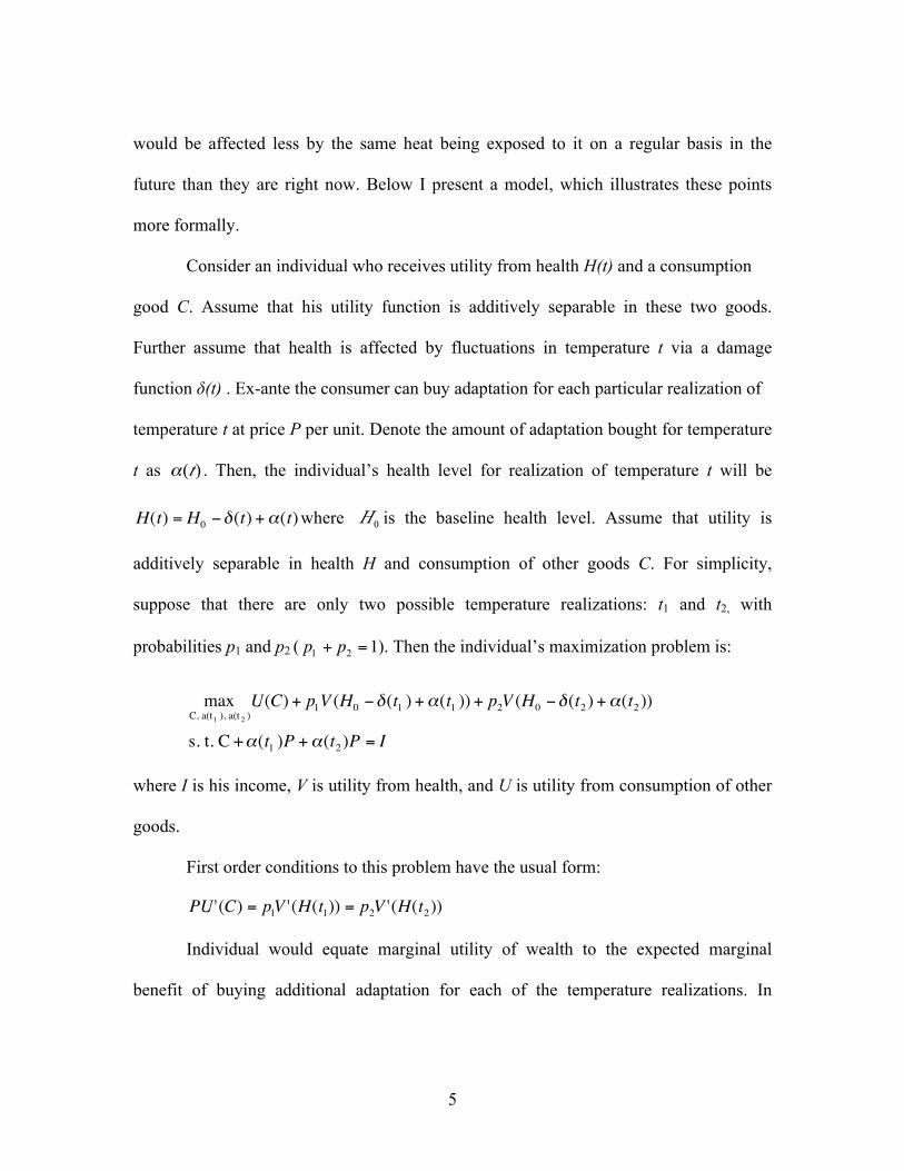
Consider an individual who receives utility from health H(t) and a consumption
good C. Assume that his utility function is additively separable in these two goods.
Further assume that health is affected by fluctuations in temperature t via a damage
function δ(t) . Ex-ante the consumer can buy adaptation for each particular realization of
temperature t at price P per unit. Denote the amount of adaptation bought for temperature
t as . Then, the individual’s health level for realization of temperature t will be
€
H(t) = H0 −δ(t) +α(t)where is the baseline health level. Assume that utility is
additively separable in health H and consumption of other goods C. For simplicity,
suppose that there are only two possible temperature realizations: t1 and t2, with
probabilities p1 and p2 (
€
p1 + p2 =1). Then the individual’s maximization problem is:
€
maxC, a(t1 ), a(t 2 )
U(C) + p1V (H0 −δ(t1 ) +α(t1 )) + p2V (H0 −δ(t2 ) +α(t2 ))
s. t. C +α(t1 )P +α(t2 )P = I
where I is his income, V is utility from health, and U is utility from consumption of other
goods.
First order conditions to this problem have the usual form:
€
PU '(C) = p1V '(H(t1)) = p2V '(H(t2))
Individual would equate marginal utility of wealth to the expected marginal
benefit of buying additional adaptation for each of the temperature realizations. In

6
particular, expected marginal utilities of health (adjusted by prices of adaptation) would
be equalized across temperature realizations. If that were not the case it would be
possible to increase utility by shifting adaptation expenditures to the state of the world
with higher expected marginal benefit.
This implies that keeping other things equal individual would spend more on
adaptation for a particular temperature realization if probability of this realization
€
pi is
higher. If some region experiences high temperature more often,
€
p2 is higher, then it
would buy more adaptation for hot weather
€
α(t2) . Hence, keeping other things equal1
damages from heat in this region will be lower (health stock
€
H(t2) will be higher) than
in the colder region, which is exposed to high temperatures only occasionally2.
Climate change in this setup could be modeled as shift in temperature distribution
with larger probability of high temperature realization:
€
p'2 > p2 where prime denotes
value in the future. As a region would start experiencing higher temperature more often3,
people in it would begin buying more adaptation equipment for the (now more likely)
high temperature realization and would suffer less from it as a result.
1 In particular, regional GDP, which might affect the ability to adapt. Population density might also have an
effect through economies of scale. In my empirical analysis I control for regional fixed effects to absorb
region specific heterogeneity. 2 In terms of empirical model this result suggest that in order to account for differential response of
different regions to the same temperature realizations, one should interact temperature with measures of
current adaptation to given temperature distribution, e.g. mean summer/winter temperatures. 3 Of course, there is likely to be some transition process since adaptation equipment (like insulation, AC
units, heat pumps etc) could last for many years. But climate change models (e.g. considered in the next
sections) suggest climate would be changing very slowly, hence I assume that people are able to adjust
their adaptation capital stock rather quickly compared to the timeframe of changes in temperature.

7
Most climate change studies ignore this adaptation response when constructing
estimates of the effect of climate change on mortality: they simply extrapolate estimates
obtained from the current temperature distribution or focus only on one particular channel
through which adaptation might take place. This is likely to bias the results in favor of
overestimating the actual costs of climate change (Mityakov and Mroz (2014)).
I propose to account for adaptation by matching the unobservable responses to
high temperature of regions which will be hot in the future to the responses to the heat of
the same intensity currently observed in hot regions. In particular, if currently cold region
C (
€
p2c is low) in the future, as a result of climate change, will be exposed to higher
temperatures more often (
€
p'2c is higher), I assume that its response to high temperature
shock (
€
t2) would be the same as for the currently hot region H for which present
exposure to heat (
€
p2H ) is similar to future exposure to heat of currently cold region (
€
p'2c ).
This would result in lower estimated damage from climate change since the
damage from high temperatures in currently warm regions (region H) is smaller than in
currently colder regions (region C) due to more adaptation bought for higher temperature
realizations.
An important technical issue here is how one should match warm regions today to
future locations. There are several ways to do this matching procedure. In the empirical
section I present the simplest empirical approach based on a linear semi-parametric
model that I use to estimate the impact of climate change on mortality in Russia.

8
1.3 Data Sources and Summary Statistics
I use monthly mortality data for 85 Russian regions per 100,000 population over
the four years 2006-2009 available from the Federal State Statistics Service. These data
represent the universe of reported deaths in each region in each month, as each death
must be registered with the police. Table 1-1 presents summary statistics on the average
monthly total mortality rates (per 100,000 population) by seasons (June-August and
December-February) for different causes of death. Mortality is also shown for three
major causes of death for adults: cardiovascular disease, respiratory disease, and
neoplasms.
The total mortality rate is 113.20 per 100,000 people per month. As in other
countries, mortality due to cardiovascular diseases is the most frequent cause of death.
Table 1-1 shows that 59.5% of overall mortality is due to that factor, representing 67.40
per 100,000 deaths. These numbers differ in winter and summer: in winter the mortality
rate is 72.05 per 100,000, in summer it is 62.92 per 100,000. On average, 5.18 people in
100,000 die in a winter month and 4.41 in a summer month from respiratory diseases.
Test of means suggest that mortality means in summer and winter are different for
cardiovascular and respiratory diseases, but not for neoplasms.
Population, GDP, and inflation data are used as controls and taken from the
Federal State Statistics Service for the same years (2006-2009). The year 2006 is used as
the base year. The average GDP per capita was 0.181 millions rubbles with standard
deviation of 0.273. The average population was 142 million people.
9
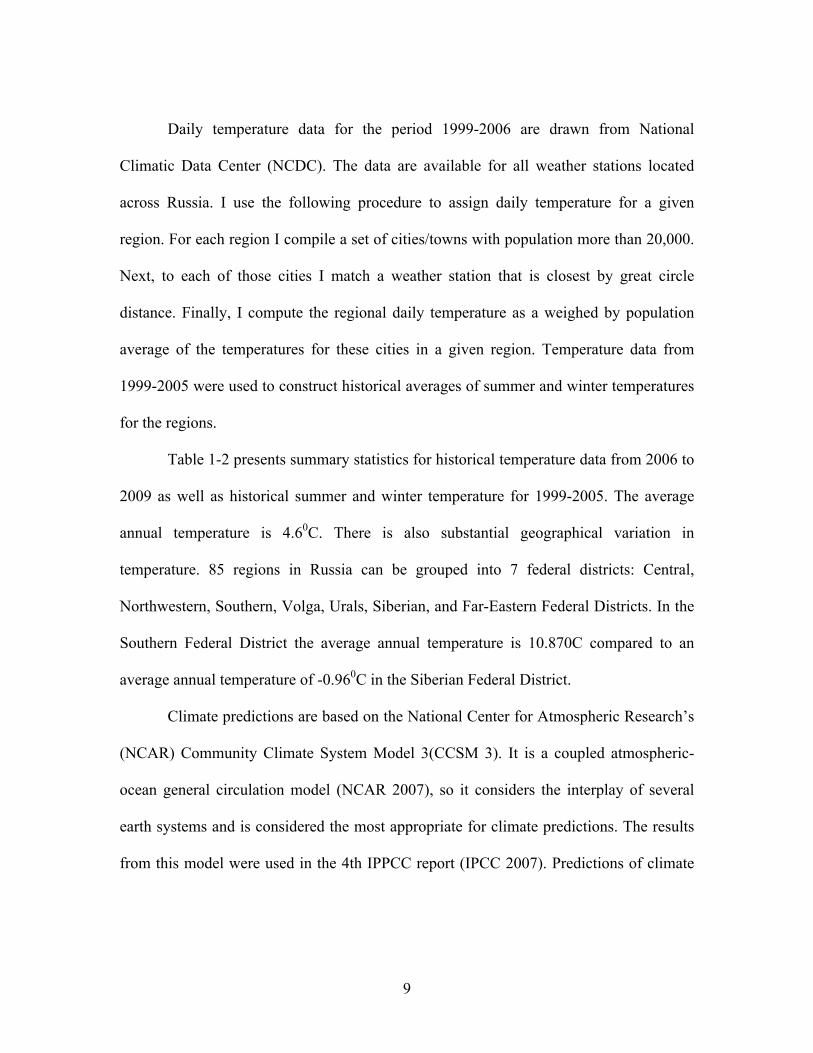
Daily temperature data for the period 1999-2006 are drawn from National
Climatic Data Center (NCDC). The data are available for all weather stations located
across Russia. I use the following procedure to assign daily temperature for a given
region. For each region I compile a set of cities/towns with population more than 20,000.
Next, to each of those cities I match a weather station that is closest by great circle
distance. Finally, I compute the regional daily temperature as a weighed by population
average of the temperatures for these cities in a given region. Temperature data from
1999-2005 were used to construct historical averages of summer and winter temperatures
for the regions.
Table 1-2 presents summary statistics for historical temperature data from 2006 to
2009 as well as historical summer and winter temperature for 1999-2005. The average
annual temperature is 4.60C. There is also substantial geographical variation in
temperature. 85 regions in Russia can be grouped into 7 federal districts: Central,
Northwestern, Southern, Volga, Urals, Siberian, and Far-Eastern Federal Districts. In the
Southern Federal District the average annual temperature is 10.870C compared to an
average annual temperature of -0.960C in the Siberian Federal District.
Climate predictions are based on the National Center for Atmospheric Research’s
(NCAR) Community Climate System Model 3(CCSM 3). It is a coupled atmospheric-
ocean general circulation model (NCAR 2007), so it considers the interplay of several
earth systems and is considered the most appropriate for climate predictions. The results
from this model were used in the 4th IPPCC report (IPCC 2007). Predictions of climate

10
change are available for several emission scenarios. I focus on the A2 “business as usual”
scenario.
Panel B in Table 1-2 shows predicted change in temperature by the end of the
century. On average Russia will experience a 3.960C increase in temperature, ranging
from 2.590C increase in Far Eastern Federal District to 5.130C increase in Urals Federal
District.
Figure 1-1 depicts the average variation in temperature across the seven
temperature categories or bins, during the 2006-2009 and 2070-2099 periods. The height
of each bar corresponds to the fraction of days in a month that the average person
experiences in each bin. Overall (according to CCSM 3, A2) there will be fewer colder
days and more warmer ones. There are some regions, however, which are predicted to
expect colder winters.
More detailed information about historical temperature, predicted temperature and
mortality rates are presented in Figures A1-A6 in the Appendix.
1.4 Results
A. Nonlinear Specifications
The effects of temperature are likely to be non-monotone. Following Deschênes
and Greenstone (2011), I consider the following flexible specification to study the
differential impact of weather on mortality at different temperature levels. I divide the
range of observed temperatures into seven 100C bins and then estimate the following
equation.

11
€
MortalityR ,m,t = βkFR ,m,t (k) + γXR ,m,t +αR +α t +k∑ αm +εR ,m,t
(1.1)
where MortalityR,m,t is the monthly mortality rate in region R, month m and year t.4 The
variables of interest are the measure of temperature, FR,m,t, capturing the exposure to the
full distribution of temperature. FR,m,t(k) is define as the fraction of days per month in a
region R, month m, and year t with daily temperature in the k-th of the seven temperature
bins.
This flexible model imposes the restriction that the temperature effect is constant
within each of the 100C bins. As usual there is a trade-off between including more bins to
allow more flexible specification and obtaining a precision in the estimates.
The parameters
€
αR ,
€
α t ,
€
αmare regional, year, and monthly fixed effects.
Regional fixed effects are included to capture unobserved time-invariant determinants of
the mortality rates, the year fixed effects control for aggregate shocks for the whole
country, and the monthly fixed effects are included to capture the seasonality in
mortality. I also include controls (X) that vary over time: regional GDP, regional GDP
squared, population and population squared.
I cluster standard errors at the regional level to capture potential serial correlation
over time. I also estimate specification (1) by GLS with weights being proportional to the
square root of population. There are two reasons for this weighting: larger populations are
likely to have more precisely estimated mortality statistics. Also I want to obtain the 4 I also considered a similar specification for log’s of mortality. The results are similar and are available
upon request.

12
effect for the average person not for the average region.
Figure 1-2 plots the results of estimating equation (1) for total mortality. I omit
the 150-250 C bin, so each βk/30 measures the estimated impact of an additional day per
month in bin k on the total mortality relative to the mortality rate associated with a day
where the average temperature is between 15-250C5. The figure 1-2 also plots the
estimated βk with 95% confidence intervals point wise.
Estimated relationship between mortality and temperature is U-shaped. For
example, the coefficient on the highest temperature (seventh) bin is 15.43. Exchanging
one month (30 days) in this range for one month (30 days) in 150-250C range would lead
to 15.43 fewer deaths per 100,000 in that month. Coefficients associated with the lower
temperature bins are smaller in magnitude, suggesting that a reduction in death rate as it
gets warmer would also be smaller. The estimates of coefficients are also shown in the
first column in Table 1-4.
B. Adaptation Response
The non-linear specification above is constructed under the assumption that all
regions respond in the same way to temperature bins. This is likely to be unrealistic, as
hotter regions might be better adapted to hot weather. Higher temperatures there are
likely to be common so one would expect that they would be better adapted to hot
weather. At the same time, my model suggests that because cold weather is rather
5 Thus, βk measures the effect on monthly mortality if the whole months (30 days) are shifted to bin k from
the omitted 15-250C bin.

13
uncommon in those areas they would tend to suffer relatively more from occasional low
temperature. Similarly, colder regions are likely to experience low temperatures more
often and hence they are likely to suffer less from it than regions where such
temperatures are less common. At the same time they would be less adapted to occasional
hot weather.
To account for this I re-estimated my regression for cold and warm regions in
Table 1-3. Results show that low-temperature bins are more harmful for warm region,
whereas high-temperature bins are more damaging for cold regions. For example, in
regions with warmer summers (column 2 in Table 1-3), the coefficient on the last bin is
14.09, suggesting that replacing one month from 150-250C to this range would lead to
14.09 more deaths per 100,000. The effect is larger (38.98 more deaths per 100,000
population) for regions with colder summers. The cold summer regions, however, are
better protected from low temperatures. The coefficient 6.92 on the [-250;-150) bin in
column (3) means that exchanging one month from 150-250C range for this bin would
lead to a 6.92 increase in mortality, in warm summer region the mortality would go up by
8.08 deaths per 100,000 population.
A similar pattern is observed if I divide regions by average winter temperature
(columns 4 and 5 in Table 1-3). The effect of low temperature is larger for warm winter
regions and effect of high temperature is smaller for these regions.
Such variation in the degree of adaptation to different temperature in different
regions is a key to my method of constructing a long-run adaptation response. In
particular, if some cold regions in the future become warmer and experience temperatures

14
similar to those currently experienced by warm regions, then the initially cold region is
likely to exhibitadaptation response in the future similar to what the warm regions do
today. The idea is to take each region in the future and construct its adaptation response
by matching its future temperature characteristics to current temperature characteristics of
other regions, using temperature responses for those regions for the given regions in the
future.
In its simplest form such a matching procedure could be done using the following
parametric specification. In my non-linear specification (1.1) I include interaction
between temperature bins and average winter and summer temperatures in a given region.
The coefficient on average summer temperature and a given (high) temperature bin
would show a differential impact of this temperature bin in high vs low summer
temperature regions. If the adaptation story presented in my model is correct then this
coefficient should be negative, i.e. the damage of high temperatures should be lower in
warmer regions, since they would be better adapted to hot weather. Similarly, the
coefficient on the interaction between average winter temperature and a (cold)
temperature bin should be positive as the effect on mortality from having low
temperature should be lower in colder regions, as they are better adapted to such weather.
I interact average winter temperature for a given region with bins for temperatures
below 150C (five bins total), and average summer temperature with bins for temperatures
above 150C (two bins total). I consider this split because low temperatures occur in the
winter and high temperatures occur in the summer. Average winter temperature indicates
the severity of cold weather experienced by a given region on a regular basis, and thus,

15
represents the degree of adaptation of a given region to cold weather. Similarly,
interactions with average summer temperature are included to measure the degree of
adaptation to heat.
€
MortalityR ,m,t = βkFR ,m,t (k) + βi1
i=1
5
∑k=1
7
∑ FR ,m,t (i) * AvWtemp+ β j2FR ,m,t (i) * AvStemp
j=6
7
∑
+γXR ,m,t +αR +αm +α t +εR ,m,t (1.2)
Estimates of equations (1.2) are presented in the second column of Table 1-4.
Consistent with the model I estimate negative coefficients on the interaction between the
sixth and seventh temperature bins and average summer temperature and the positive
coefficient for the interaction between other bins and winter temperatures. The estimates
suggest that the effect of low temperature on mortality is smaller in regions with lower
average winter temperature, while the effect of high temperature on mortality is smaller
in regions with high average summer temperature.
Figure 1-6 shows the response functions using specification (1.2) for two regions:
“Cold region” and “Hot region. “Cold region” is a region with cold winters (-23.50C) and
cool summer (140C). “Hot region” is a region with warmer winters (-1.50C) and hot
summers (240C). It is evident from the figure that a “Hot region” is better adapted to hot
weather; the effect of the last temperature bin is smaller. There will be 8.43 more deaths
if 30 days in the 150-250C bin are exchanged for 30 days in the hottest bin. There will be
almost 50 more deaths in a “Cold region”. A “Cold region”, however, is better adapted to
low temperature: the effect of lower temperatures is less damaging in this region relative
to the “Hot region”.

16
Figure 1-7 depict the effects of temperature on mortality for the coldest region,
the warmest region, a moderate region and the adaptation curve. The adaptation curve is
an envelope of all response functions. The adaptation curve shows the effect of
temperature on mortality if all regions were to look like the warmest region today in
summer and the coldest region today in winter.
C. Prediction
Specification in equation (1.2) is linear in average summer and winter
temperatures, so it extrapolates adaptation for warm regions beyond currently observed
levels. (e.g. for southern regions summer temperatures would go up in the future, which
from specification (1.2) would result in further adaptation according to negative
estimated coefficients on interaction between average summer temperature and
temperature bins above 150C). However, one cannot be sure that such adaptation
tendencies will be possible. To avoid this extrapolation of adaptation response when I
compute predictions, I restrict average summer temperature not to exceed historically
observed maximum of around 250C. This allows for colder regions to go along the
adaptation path suggested by currently hot regions, but restricts currently hot regions to
not over-adapt. In effect this guarantees that my estimates of adaptation would likely to
provide a lower bound for possible total adaptation response.
Furthermore I assume that colder regions do not lose their ability to adapt to cold
weather. Hypothetically it is possible for the same cold temperature bin in the future to be
more damaging to currently cold region than it is today.
17
It should also be noted that in these calculations I explicitly omit the impact of
GDP growth on changes in mortality since I want to estimate the impact of temperature
changes per se.
To compute changes in mortality I use the following procedure.
1. Use current temperature data and estimated coefficients of
specifications (1.1) (no adaptation) and (1.2) (adaptation) to compute
predicted mortality in 2006-2009.
2. Use predictions about future temperature data (both bins and
interactions) to compute predicted mortality in the future.
3. Calculate the difference between the two.
Table 1-5 contains the results of my calculations. We see that the model without
adaptation predicts additional eight deaths per year per 100,000 population between
2070-2099 (or 0.5 percent increase in mortality) due to the temperature change predicted
be Hadley model. However, once an adaptation response is allowed according to equation
(1.2) we see that in fact Russia is likely to benefit in terms of decreased mortality: ten
fewer deaths per year per 100,000 population between 2070-2099, which amounts to one
percent decrease in mortality. Almost all districts would actually gain from climate
change in terms of mortality if the model with adaptation used.
The Volga Federal District has the biggest difference between predictions from
those two models. This district is one of the coldest districts now. The model without
adaptation predicts increased mortality by 9.97 more death per year per 100,000
population. The model with adaptation, however, predicts decreased mortality by 16.10

18
fewer deaths per year per 100,000 population. According to climate change model
predictions (CCSM 3, A2) summer will be hotter, so a model without adaptation would
predict a large increase in deaths. But this does not have to be the case. Since climate
change will unfold gradually, people could adapt more effectively to new hotter summer.
As a result, there will be fewer deaths from high temperature. The large improvement in
mortality is also due to winter being hotter as well, and so there will be fewer deaths from
low temperature.
Another big difference in predicted mortality occurs in the Southern Federal
District, which is originally the warmest district. The model without adaptation predicts
increased mortality by 21.20 death per 100,000 population. However, the model with
adaptation predicts decreased mortality. There are two reasons for that. First, the model
with adaptation predicts fewer deaths from heat in warm regions, since, in essence, it is
estimating effect for colder and warmer regions separately. So, warming is not as harmful
as predicted using model without adaptation. This explains why mortality is predicted to
be lower in the model with adaptation vs. the model without adaptation.
Second, the climate change model predicts that there will be fewer cold days in
those regions. And colder weather is particularly damaging to warm regions. This again
would decrease future mortality in warm regions, which explains why the model with
adaptation actually predicts some gains for Southern district.
1.5 Robustness Checks
A. Alternative Climate Change Measures

19
This subsection presents the result if cooling and heating degree days are used as
a measure of climate/weather instead of temperature. To calculate these variables
temperature of 180C is used as a base. Specifically, on a given day, the number of cooling
degree days equals the day’s mean temperature minus 180C for days where the mean is
above 180C and zero for days when the mean is below 180C. Similarly, a day’s heating
degree days is equal 180C minus its mean for days where the mean is below 180C and
zero otherwise. So, a day with a mean temperature of 200C would contribute two cooling
degree days and zero heating degree days, while a day with a mean of -100C would
contribute zero cooling degree days and 28 heating degree days. To compute the
relationship between heating and cooling degree and mortality I sum the number of
heating degree days (hdd) and cooling degree days (cdd) separately over the month.
I include heating degree days (hdd), cooling degree days (cdd) and their squares
instead of the fraction
€
FRmt (k) in the specification (1.1), model without adaptation and
estimate the following equation:
€
MortalityRmt = β1cdd + β2cdd2 + β3hdd + β4hdd
2 + γXRmt +αR +αm +α t (1.3)
where, as before, MortalityR,m,t is the monthly mortality rate in region, month m and year
t. The parameters , , are regional, year, and monthly fixed effects. X are
varying over time controls: regional GDP, regional GDP squared, population and
population squared.
Next, I estimate the following model with adaptation, which is similar to the
specification (1.2), where average winter and summer temperatures were used as a
measure of adaptation:

20
€
MortalityRmt = β1cdd + β2cdd2 + β3hdd + β4hdd
2 + γXRmt +αR +αm +α t +
β5cdd * AvStemp+ β6cdd2 * AvStemp+ β7hdd * AvWtemp+ β8hdd
2 * AvWtemp
(1.4)
Table 1-6 shows the predicted change in mortality. To compare with the previous
results, in first two columns I repeat the predicted change from equations (1.1) and (1.2).
Columns (3) and (4) show the predicted change in mortality using new measure of
weather severity, using estimates from equations (1.3) and (1.4) respectively. As before, a
model without adaptation predicts an increase in mortality rates, however, the model with
adaptation predicts a decrease in mortality. Magnitudes of the effects remain similar,
although the effects are less precisely estimated.
In Table 1-7 I match adaptation response of regions using the mean number of
heating and cooling degree-days in winter and summer respectively instead of
temperature. I again find smaller and less precise estimated effects, but still negative,
meaning reduction in mortality by the end of the century.
B. Hereditary Component in Adaptation
My estimates of adaptation response while comprising the whole range of
adaptation techniques do not pinpoint the particular adaptation channel. They implicitly
assume that adaptation techniques available in warmer (southern) regions can easily be
used by resident of currently colder (nothern) regions. What if lower response to heat in
the south were hereditary, i.e. over the years as a result of selection and evolution people
living there have accumulated some tolerance to heat. In that case such an adaptation

21
option would be difficult to imitate by residents of northern regions. To see to what
extent my findings regarding adaptation response may be driven by those hereditary heat
tolerance effects,I repeat my estimations excluding the ethnic southern regions. The idea
is that if hereditary component of adaptation is very important then the estimated effect
omitting those regions should be much smaller. I find that my estimates are virtually
unchanged. Results are shown in Table 1-8. This suggests that adaptation patterns I
describe are unlikely to be driven by hereditary predisposition to heat tolerance and thus
can be widely adapted by residents of other regions.
C. Alternative windows for temperature impact
In the main results section 1.4 above we considered the impact of current month’s
average temperature on mortality in a given month. Such specification assumes that only
temperatures observed in a given month might affect this month’s mortality. However, it
could be argued that one-month window might be not long enough to account for the full
damage from temperature. In this section I consider the effect on monthly mortality of
temperature averaged over time windows longer than just one month. Namely, I related
current month’s mortality rate to temperature averaged over previous two and three
months. The results presented in Table 1-9 indicate similar pattern as for baseline (one-
month window) results.
The magnitudes of the effects are somewhat smaller than under the baseline (e.g.
under no adaptation costs are around one percent in the three month window specification
and there are even slight benefits in two month specification). However, in both cases

22
when I allow for adaptation I estimate considerable benefits from climate change in terms
of reduced mortality.
1.6 Conclusion
In this chapter I investigate the mortality response to climate change in Russia. I
find a non-linear U-shaped relation between temperature and mortality in Russia. I
further look at the differential impacts of temperature in warmer and colder regions. On
the basis of this analysis, I propose a new approach to account for adaptation response to
climate change in the long-run. Specifically, I assume that as currently cold regions start
experiencing warmer weather more regularly they will adapt similar extreme temperature
adaptation techniques (and would thus have similar responses) as the regions that are
currently warm. I show that this approach make a large difference for the estimates of the
impact of climate change on mortality in Russia. In particular, the model without
adaptation response predicts that mortality will increase in Russia as a result of climate
change. Once adaptation is taken into account, however, I find considerable and
statistically significant reductions in mortality due to climate change.

23
1.7 Tables Table 1-1: Mortality Rates by Cause of Death
Variable All months Winter Summer Monthly Mortality per 100,000 All causes of death 113.20 118.85 108.05 (35.16) (37.73) (32.28) Cardiovascular disease 67.40 72.05 62.92 (23.05) (24.83) (20.49) Respiratory diseases 4.91 5.18 4.41 (2.39) (2.61) (2.10) Neoplasms 15.91 15.88 15.90 (4.85) (4.85) (4.75) Observations 4032 1008 1008 Notes: Standard deviations are in parentheses. Source: Russian Federal State Statistics Service (http://gks.ru)

24
Table 1-2: Summary Statistics for Temperature in 0C
Mean Min Max Panel A. Historical temperature data (2006-2009)
All districts 4.63 -40.31 28.54 By districts 1. Central FD 6.47 -16.42 22.55 2. Northwestern FD 3.93 -22.8 21.21 3. Southern FD 10.87 -13.68 28.54 4. Volga FD 5.17 -20.29 25.25 5. Urals FD 1.27 -34.15 22.34 6. Siberian FD 0.96 -34.25 23.61 7. Far Eastern FD -0.51 -40.31 23.25
Panel B. Predicted change, CCSM 3 A2 (2070-2099) All districts 3.96 15.94 4.12 By districts 1. Central FD 3.94 12.46 7.38 2. Northwestern FD 3.63 13.41 4.14 3. Southern FD 4.22 15.04 4.11 4. Volga FD 4.28 12.52 3.59 5. Urals FD 5.13 20.58 2.70 6. Siberian FD 3.79 16.24 1.21 7. Far Eastern FD 2.59 15.94 0.00
Panel C. Historical temperature data (1999-2005) Average Winter Temp -9.62 6.89 -34.83 Average Summer Temp 18.38 2.51 12.34 Notes: Historical temperature data are taken from National Climatic Data Center (NCDC). Predicted changes defined as difference between 2070-2099 temperatures from CCSM 3 scenario A2 and 2006-2009 temperatures.

25
Table 1-3: Nonlinear Effect of Temperature on Monthly Mortality in Russia by
Regions
(1) (2) (3) (4) (5)
VARIABLES All
regions Hot
summer Cold
summer Hot winter Cold
winter [-41; -25) 4.741 15.991** 3.286 41.684*** 11.337** (3.424) (6.534) (3.579) (7.956) (4.818) [-25; -15) 8.145*** 8.818*** 6.925*** 12.762*** 12.702*** (1.752) (3.007) (2.298) (4.047) (3.004) [-15; -5) 6.042*** 4.399* 8.071*** 6.059** 11.512*** (1.926) (2.511) (2.816) (2.660) (3.583) [-5; 5) 5.221*** 6.188*** 4.536* 2.156 10.056*** (1.451) (2.049) (2.308) (2.098) (3.615) [5; 15) 4.917*** 4.765** 3.019 1.789 3.463 (1.407) (1.984) (2.280) (1.806) (2.718) [15; 25) – – – – – [25; 29) 15.343*** 14.094*** 38.978*** 17.362*** 22.354*** (2.065) (2.384) (7.477) (2.151) (7.642) Observations 4,032 1,776 2,256 2,304 1,728 Notes: Dependent variable is monthly mortality in Russian regions for years 2006-2009. Explanatory variables represent fractions of days in a given month in a particular temperature bin. Warm summer and warm winter are regions with average summer/winter temperature higher than the country averages; cold summer and cold winter are regions with summer/winter temperature below the country averages. Robust standard errors in parentheses are clustered at the regional level. Regional GDP, population and their squares as well as regional, year, and monthly fixed effects are included but not reported. ***, **, and * indicate significance at 1%, 5%, and 10% respectively

26
Table 1-4: Nonlinear Effect of Temperature on Monthly Mortality in Russia
VARIABLES (1) (2) [-41; -25) -0.117 20.113** (3.352) (8.244) [-25; -15) 3.289* 20.115*** (1.834) (4.482) [-15; -5) 1.188 10.943*** (1.653) (3.114) [-5; 5) 0.363 5.710*** (1.214) (1.978) [5; 15) -– -– [15; 25) -4.964*** 5.099 (1.402) (7.841) [25; 29) 10.470*** 94.454*** (2.300) (17.614) [-41; -25)*Winter – 0.837*** (0.252) [-25; -15)*Winter – 0.932*** (0.231) [-15; -5)*Winter – 0.622*** (0.197) [-5; 5)*Winter – 0.558*** (0.170) [5; 15)*Winter – 0.236 (0.174) [15; 25)*Summer – -0.560 (0.393) [25; 29)*Summer – -3.564*** (0.792) Observations 4,032 4,032 Notes: Dependent variable is monthly mortality in Russian regions for years 2006-2009. Explanatory variables represent fractions of days in a given month in a particular temperature bin. Robust standard errors in parentheses are clustered at the regional level. Regional GDP, population and their squares as well as regional, year, and monthly fixed effects are included but not reported. ***, **, and * indicate significance at 1%, 5%, and 10% respectively.

27
Table 1-5: Predicted Change in Annual Mortality
No Adaptation With Adaptation All districts 8.08 -10.08 [1.98; 13.94] [-18.94; -0.53] By districts 1. Central FD 11.08 -7.21 [3.77; 18.28] [-19; 3.32] 2. Northwestern FD -0.93 -10.93 [-7.49; 4.40] [-18.20; -2.65] 3. Southern FD 21.20 -9.40 [11.55; 31.50] [-23.39; 5.78] 4. Volga FD 9.97 -16.10 [2.13; 16.67] [-27.71; -4.45] 5. Urals FD 3.66 -12.78 [-4; 11.26] [-24.14; -1.12] 6. Siberian FD 3.65 -9.74 [-1.73; 9.38] [-18.46; -0.46] 7. Far Eastern FD -0.42 -5.03 [-4.04; 3.06] [-12.52; 0.97] Notes: 95% confidence intervals are in brackets computed using bootstrap with 1000 repetitions; predictions are for CCSM 3, A2 climate model scenario. First column shows predictions using specification (1.1) with no adaptation, second column using specification (1.2) with adaptation. All averages are weighted by population.

28
Table 1-6: Predicted change in annual mortality: Heating and Cooling degree days
Temperature Bins Heating and Cooling degree days No Adaptation With adaptation No Adaptation With adaptation All districts 8.08 -10.08 6.03 -9.05 [1.98; 13.94] [-18.94; -0.53] [-0.83; 13.93] [-19.10; 1.36] 1. Central FD 11.08 -7.21 8.05 -8.71 [3.77; 18.28] [-19; 3.32] [-0.17; 17.41] [-20.02; 2.57] 2. Northwestern -0.93 -10.93 -6.66 -16.55 FD [-7.49; 4.40] [-18.20; -2.65] [-12.72; -0.71] [-24.08; -9.16] 3. Southern FD 21.20 -9.40 18.86 10.21 [11.55; 31.50] [-23.39; 5.78] [1.06; 38] [-20.91; 42.91] 4. Volga FD 9.97 -16.10 5.80 -20.69 [2.13; 16.67] [-27.71; -4.45] [-1.65; 15.13] [-32.32; -9.71] 5. Urals FD 3.66 -12.78 1.99 -17.74 [-4; 11.26] [-24.14; -1.12] [-5.67; 10.40] [-27.20; -7.73] 6. Siberian FD 3.65 -9.74 5.02 -10.66 [-1.73; 9.38] [-18.46; -0.46] [-0.58; 10.86] [-18.37; -3.31] 7. Far Eastern FD -0.42 -5.03 3.27 -2.56 [-4.04; 3.06] [-12.52; 0.97] [-0.40; 7.06] [-7.72; 1.64] Notes: 95% confidence intervals in brackets are computed using bootstrap with 1000 repetitions; All specifications use predicted temperature data from CCSM 3, A2 climate model scenario. First column uses non-linear specification (1.1) for temperature-mortality relation with no adaptation; second column uses specification (1.2) with adaptation on the basis of average winter and summer temperatures as described in the main text. Third and fourth columns use cooling/heating degree days-mortality relation (1.3) and (1.4) without and with adaptation respectively. All averages are weighted by population.

29
Table 1-7: Predicted Change in Annual Mortality:
Cooling and Heating Degree Days as a Measure of Adaptation
Fractions CDD/HDD All districts -4.99 -5.67 [-12.63; 4.12] [-14.51; 3.34] 1. Central FD -2.33 -6.67 [-12.01; 8.24] [-16.72; 3.87] 2. Northwestern -11.27 -18.11 FD [-17.79; -3.42] [-25.67; -10.10] 3. Southern FD 1.68 21.72 [-10.36; 15.06] [-7.35; 48.42] 4. Volga FD -6.73 -13.71 [-17.15; 3.97] [-23.21; -3] 5. Urals FD -6.65 -14.21 [-16.56; 4.54] [-22.59; -4.47] 6. Siberian FD -3.63 -6.72 [-11.11; 4.58] [-13.02; 0.45] 7. Far Eastern FD -10.09 -8.58 [-16.14; -4.14] [-13.86; -2.78] Notes: 95% Confidence intervals are in brackets computed using bootstrap with 1000 repetitions; In both columns cooling and heating degree days were used as a measure of adaptation. First column predictions are for temperature bins specification (1.2); Second column predictions are for the cooling and heating degree days specification (1.4). All averages are weighted by population

30
Table 1-8: Predicted Change in Annual Mortality
(Southern Ethnic Regions Dropped)
All regions Southern Ethnic Regions Dropped No Adaptation With adaptation No Adaptation With adaptation All districts 8.08 -10.08 7.74 -13.64 [1.98; 13.94] [-18.94; -0.53] [1.26; 13.52] [-21.96; -4.01] 1. Central FD 11.08 -7.21 11.14 -11.84 [3.77; 18.28] [-19; 3.32] [3.69; 18.67] [-22.05; -0.48] 2. Northwestern -0.93 -10.93 -1.19 -13.67 FD [-7.49; 4.40] [-18.20; -2.65] [-6.95; 4.54] [-20.82; -5.72] 3. Southern FD 21.20 -9.40 21.58 -12.36 [11.55; 31.50] [-23.39; 5.78] [10.65; 33.50] [-30.92; 6.31] 4. Volga FD 9.97 -16.10 10.07 -21.11 [2.13; 16.67] [-27.71; -4.45] [2.67; 17.63] [-31.75; -8.12] 5. Urals FD 3.66 -12.78 3.56 -17.36 [-4; 11.26] [-24.14; -1.12] [-3.92; 11.09] [-27.91; -5.94] 6. Siberian FD 3.65 -9.74 4.21 -12.15 [-1.73; 9.38] [-18.46; -0.46] [-1.08; 9.83] [-19.74; -3.32] 7. Far Eastern FD -0.42 -5.03 -0.06 -6.36 [-4.04; 3.06] [-12.52; 0.97] [-3.46; 3.40] [-12.51; 0.87] Notes: 95% confidence intervals in brackets are computed using bootstrap with 1000 repetitions; All specifications use predicted temperature data from CCSM 3, A2 climate model scenario. First column uses non-linear specification (1.1) for temperature-mortality relation with no adaptation; second column uses specification (1.2) with adaptation on the basis of average winter and summer temperatures as described in the main text. Third and fourth columns use cooling/heating degree days-mortality relation (1.3) and (1.4) without and with adaptation respectively. All averages are weighted by population.

31
Table 1-9: Predicted Change in Annual Mortality Using Different Temperature
Impact Windows
2 months window 3 months window No Adaptation With adaptation No Adaptation With adaptation All districts -0.309 -6.257 1.838 -4.603 [-7.408; 6.280] [-15.056; 2.817] [-5.745; 9.156] [-14.994; 6.000] 1. Central FD 0.498 -2.917 1.483 -2.436 [-8.210; 8.071] [-13.628; 9.166] [-7.813; 10.876] [-15.45;1 10.418] 2. Northwestern -6.228 -11.692 -4.020 -7.847 FD [-12.95; -0.407] [-19.15; -4.562] [-10.919; 2.267] [-16.058; 0.482] 3. Southern FD 7.698 -7.570 6.999 -11.266 [-3.159; 18.479] [-25.18; 11.405] [-6.345; 19.683] [-34.391; 13.522] 4. Volga FD 1.176 -8.364 2.472 -6.985 [-7.454; 9.145] [-19.677; 4.189] [-6.383; 11.606] [-21.185; 7.385] 5. Urals FD -6.332 -9.500 -1.550 -4.601 [-14.941; 1.745] [-21.566; 3.584] [-10.645; 7.592] [-16.325; 9.459] 6. Siberian FD -2.595 -8.494 2.856 -1.037 [-8.264; 2.572] [-17.227; 0.980] [-2.837; 8.414] [-10.113; 8.488] 7. Far Eastern FD -1.755 3.779 0.068 3.997 [-5.410; 1.392] [-3.658; 13.218] [-0.509; 5.003] [-4.611; 14.078] Notes: 95% confidence intervals in brackets are computed using bootstrap with 1000 repetitions; All specifications use predicted temperature data from CCSM 3, A2 climate model scenario. First column uses non-linear specification (1.1) for temperature-mortality relation with no adaptation; second column uses specification (1.2) with adaptation on the basis of average winter and summer temperatures as described in the main text. Third and fourth columns use cooling/heating degree days-mortality relation (1.3) and (1.4) without and with adaptation respectively. All averages are weighted by population.

32
1.8 Figures Figure 1-1: Historical and Predicted Temperature by Bins
Notes: 7 categories are 10 degrees bins. Historical temperature data are taken from National Climatic Data Center (NCDC). Predicted temperature data are taken from CCSM 3 model, A2 scenario.
0
0.05
0.1
0.15
0.2
0.25
0.3
[-‐41;-‐25) [-‐25;-‐15) [-‐15;-‐5) [-‐5;5) [5;15) [15;25) [25;29)
Historical data (2006-‐2009) Predicted temperature (2070-‐2099)

33
Figure 1-2: Estimated Relationship Between Monthly Mortality Rate per 100,000
From All Causes and Average Daily Temperature
Notes: This figure plots the response function between monthly mortality from all causes and daily mean temperature. This is obtained from estimating the equation (1.1). This response function is normalized with the 150-250C cell, so each βk corresponds to the estimated impact of an additional day in bin k on the monthly mortality rate (i.e. deaths per 100,000) relative to the mortality rate associated with a month where the average temperature is between 150-250C. This figure also plots the estimated βk’s plus and minus two standard error of the estimates. Figure 1-3: Estimated Relationship Between Monthly Mortality Rate per 100,000
From Cardiovascular Diseases and Average Daily Temperature
Notes: This figure plots the response function between monthly mortality from cardiovascular diseases and daily mean temperature. This is obtained from estimating the equation (1.1). This response function is normalized with the 150-250C cell, so each βk corresponds to the estimated impact of an additional day in bin k on the monthly mortality rate (i.e. deaths per 100,000) relative to the mortality rate associated with a month where the average temperature is between 150-250C. This figure also plots the estimated βk’s plus and minus two standard error of the estimates.
-‐4 0 4 8 12 16 20 24
[-‐41; -‐25) [-‐25;-‐15) [-‐15;-‐5) [-‐5;5) [5;15) [15;25) [25;29)
Monthly deaths from all causes, per 100,000
+2 StD Error
-‐2 StD Error
-‐4
0
4
8
12
16
[-‐41; -‐25) [-‐25;-‐15) [-‐15;-‐5) [-‐5;5) [5;15) [15;25) [25;29)
Monthly deaths from cardiovascular diseases, per 100,000
+ 2 StD Error
-‐2 StD Error

34
Figure 1-4: Estimated Relationship Between Monthly Mortality Rate per 100,000
From Respiratory Diseases and Average Daily Temperature
Notes: This figure plots the response function between monthly mortality from respiratory diseases and daily mean temperature. This is obtained from estimating the equation (1.1). This response function is normalized with the 150-250C cell, so each βk corresponds to the estimated impact of an additional day in bin k on the monthly mortality rate (i.e. deaths per 100,000) relative to the mortality rate associated with a month where the average temperature is between 150-250C. This figure also plots the estimated βk’s plus and minus two standard error of the estimates.
Figure 1-5: Estimated relationship between monthly mortality rate per 100,000
from neoplasms and average daily temperature
Notes: This figure plots the response function between monthly mortality from neoplasms and daily mean temperature. This is obtained from estimating the equation (1.1). This response function is normalized with the 150-250C cell, so each βk corresponds to the estimated impact of an additional day in bin k on the monthly mortality rate (i.e. deaths per 100,000) relative to the mortality rate associated with a month where the average temperature is between 150-250C. This figure also plots the estimated βk’s plus and minus two standard error of the estimates.
-‐1 -‐0.5 0
0.5 1
1.5 2
2.5
[-‐41; -‐25) [-‐25;-‐15) [-‐15;-‐5) [-‐5;5) [5;15) [15;25) [25;29)
Monthly deaths from respiratory diseases, per 100,000
+ 2 StD Error
-‐ 2 StD Error
-‐1 -‐0.5 0
0.5 1
1.5 2
2.5 3
[-‐41; -‐25) [-‐25;-‐15) [-‐15;-‐5) [-‐5;5) [5;15) [15;25) [25;29)
Month deaths from neoplasms,per 100,000 +2 StD Error -‐2 StD Error

35
Figure 1-6: Monthly Deaths for Adults for all causes of death, per 100,000
(relative to cell 150-250C)
Notes: This figure plots the response function between monthly mortality from all causes and daily mean temperature. This is obtained from estimating the equation (1.2). This response function is normalized with the 150-250C cell so each βk corresponds to the estimated impact of an additional day in bin k on the monthly mortality rate (i.e. deaths per 100,000) relative to the mortality rate associated with a month where the average temperature is between 150-250C.. Figure 1-7: Monthly Deaths for Adults for all causes of death, per 100,000
(relative to cell 150-250C)
Notes: This figure plots the response function between monthly mortality from all causes and daily mean temperature. This is obtained from estimating the equation (1.2). This response function is normalized with the 150-250C cell so each βk corresponds to the estimated impact of an additional day in bin k on the monthly mortality rate (i.e. deaths per 100,000) relative to the mortality rate associated with a month where the average temperature is between 150-250C.
-‐20
-‐10
0
10
20
30
40
50
60
<-‐25 [-‐25;-‐15) [-‐15;-‐5) [-‐5;5) [5;15) [15;25) >25
Cold region Hot region
-‐20
-‐10
0
10
20
30
40
50
60
<-‐25 [-‐25;-‐15) [-‐15;-‐5) [-‐5;5) [5;15) [15;25) >25
Cold Hot Moderate Adaptation Curve

36
CHAPTER 2
ADAPTATION TO CLIMATE CHANGE THROUGH
MIGRATION
2.1 Introduction
In this chapter I assess migration as an adaptation mechanism to climate change.
This chapter makes the following three contributions to the literature.
First, most existing estimates adopt a hedonic approach, which extrapolates
marginal valuations for currently observed temperature. In this chapter I analyze a
structural discrete location choice model where the choice depends on potential earnings,
moving costs, climate and non-climate specific location attributes. On the basis of this
model I can compute the counterfactual responses in terms of both migration decisions
and welfare to non-marginal changes in temperature, predicted by most climate models.
Second, in this model I account explicitly for general equilibrium effects of
migration on population density, which most existing studies ignore. It could be argued
that as climate change induces migratory flows, population density, which affects
individual level locational choices, would be changing as well. To solve the inherent
endogeneity of population density I use geological structure variables as instruments.
Particularly, I utilize non-sedimentary bedrock prevalence, which makes the construction
of high buildings possible, as an instrument for population density. Rosenthal and Strange

37
(2008) used similar instruments for population density in their analysis of human capital
agglomeration effects.
Third, all existing studies of migratory response to climate change rely on results
from the sample of people who actually choose to move. This considerably limits the
applicability of those estimates to general population. In this chapter I model the selection
process into being a mover as a function of individual level observables and present the
estimates. This model is more likely to be representative of the general population
migration patterns.
This study is related to the literature on the determinants of migration, particularly
regarding the impact of climate amenities on individual location decisions. As was
already mentioned above most papers in this field use hedonic approaches, which
estimate the marginal willingness to pay for a small change in climate variables
(Blomquist et al. (1988), Gyourko and Tracy (1991), Smith (1983) and Albouy et al.
(2011)).
Marginal willingness to pay does not incorporate moving costs in the individual
decision. It simply represents the marginal change in utility in response to an
infinitesimal change in climate or other amenity assuming that individuals do not change
their locations. A model of discrete location choice allows the computation of the
responses to “large” shocks to climate as well as explicitly accounting for moving costs.
Some papers in the literature already use structural models e.g. Cragg and Kahn
(1997) and Sinha and Cropper (2013). These papers, however, look only at people who
move and do not include general equilibrium effects. In this study I explicitly account for
38
general equilibrium effects for population density. My approach in this regard is
somewhat similar to Timmins (2007), who accounts for general equilibrium effects in his
analysis of migration decisions in Brazil.
The estimates from my model suggest that climate characteristics are indeed
important determinants of individual locational choices: people tend to avoid locations
with temperature extremes. At the same time I find some heterogeneity in response.
Older and more educated people care more about climate amenities. Moving costs are
estimated to be larger for younger and less educated people.
On the basis of this model I am able to calculate the welfare costs of climate
change and induced migratory responses. I find that climate change would result in
considerable welfare losses: to attain present day level of utility, in the absence of
migration, households would require an increase in their incomes by 30 percent on
average. Those costs are not uniform: some areas in the south (particularly in Florida and
some densely populated MSA’s on the East coast) would require compensation above 50
or even 60 percent. At the same time some sparsely populated areas in the North
(Dakotas, Wisconsin, Michigan etc) would actually see some benefits, with their
residents being willing to pay up to 20 percent of their current incomes to see climate
change happening.
I show that migration smoothes out those extremes and is particularly beneficial
for areas which are hit particularly hard, with the costs going down by more than 5
percentage points of overall compensating variation (which amount to more than 10
percent of total welfare losses due to climate change). At the same time the gains from

39
climate change would be reduced in Northern locations, as they would experience
migratory inflows from the rest of the country and face increases in population density.
For the whole country, on average, the gains from migration are positive but net effects
are somewhat modest.
2.2 Model
Consider an economy populated by K types of individuals differing in their
education and age. Let Nk denote the number of people of particular type k: k=1,…,K.
Assume that the country is divided into J locations, which differ in their climatic as well
as economic characteristics.
Let b(i) be the initial location for individual i. Assume that at a given moment in
time only some individuals make locational choices; I call them potential movers. I
assume that individuals are assigned into this category on the basis of some function
observable individual characteristics, structural parameters and unobserved
characteristics.
The probability an individual (in group k) with observed characteristics Si is a
mover is given by
€
π i = Fk (Si ,β) (2.1)
where Fk is type k specific function taking values between 0 and 1, and βk is the (group k

40
specific) structural parameter showing the impact of characteristics S on the propensity
to move.6
In my analysis I consider Si to be marital status (MSi) and number of children
(NChi) and specify Fk to be the following logit function:
€
π i = F (MSi ,NChi ) =exp(β MSi + βNChNChi + βconst )1+ exp(β MSi + βNChNChi + βconst )
(2.2)
Conditional on being a potential mover, individual i decides where to live and
how to spend her income Wi,j earned in the location j of her choice. This model abstracts
from the individual’s labor-leisure decision, as it considers only the wage (Wi,j) that
individual i could earn in location j. A potential mover could choose to remain in the
location she currently resides.
The utility that an individual of type k receives in location j is a function of the
(wage) income received in that location Wi,j, the moving costs (f(db(i),j)) that the
individual would have to pay to live in a location j, given she was in location b(i) in the
previous period, vectors of climate and non-climate local attributes (Cj), the congestion
or agglomeration effect of equilibrium population density ( ), an unobserved (to the
econometrician) set of local attributes
€
ε j , and an idiosyncratic shock
€
ν i, j .
I assume that the utility individual i of type k receives from living in location j is
given by:
€
Ui, j = αw lnWb( i), j +αd f (db(i), j ) +αCg(C j ) +αΔ lnΔ j +ε j +ν i, j (2.3)
6 To simplify notation I omit group specific subscript k in the description of individual maximization
problem presented below, where this does not cause confusion.
€
Δ j

41
Stayers receive the utility associated with their current place of residence and
potential movers choose the location that gives them the highest utility. Assuming that an
individual specific shock is distributed i.i.d. Type-I extreme, the probability that a mover
who is a type k individual will choose to live in location j is given by
€
Pi. j (W ,d,C,Δ;α) = Pr(lnVi, j ≥ lnVi,l , ∀j ≠ l) =
=exp(αCg(C j ) +αΔ lnΔ j +αd f (db( i), j ) +αw lnWi, j +ε j )
exp(αCg(Cl ) +αΔ lnΔ l +αd f (db(i),l ) +αw lnWi,l +ε l )l=1
J
∑ (2.4)
Replacing all variables that vary only by location j with a location specific fixed
effect θj, we can rewrite migration equation (2.4) as:
€
Pi, j (W ,d;α,θ) =exp(θ j +αd f (db( i), j ) +αw lnWi, j )
exp(θ j +αd f (db( i),l ) +αw lnWi,l )l=1
J
∑ (2.5)
where
€
θ j (C j ,Δ j;α) = αCg(C j ) +αΔ lnΔ j +ε j (2.6)
Those fixed effects could be interpreted as an average utility (quality of life index) of
living in a given location j abstracting from individual wage and distance cost of moving
there.
The population density Δj in location j is determined by
€
Δ j =
(1−π i )i:b( i)= j∑ + π i Pi, j
i∑
Land j (2.7)
where expression in the numerator is population choosing location j. It consists of people
who were in location j in previous period (b(i)=j) and were not potential movers, and all
42
those potential movers from all locations who chose to live in location j. Landj is land
area of location j.
Note that here there is a fixed point problem, since population density Δj is both a
determinant of individual’s location choice and simultaneously it is the outcome of
individual location choice decisions in equilibrium. Properties of this system are
discussed in Bayer and Timmins (2005, 2007). They show that an equilibrium always
exists and is unique provided the coefficient on density
€
αΔ is negative.
2.3 Estimation
Estimation proceeds in two steps. First, I estimate coefficients on individual
specific factors determining locational choice (wage, moving costs), and selection into
being a potential mover as well as location specific fixed effects. In particular, using
observed individual locational choices c(i), initial locations b(i), as well as individual
wages Wij and observed population density Δj, I can construct the following likelihood
function for individuals of type k:
€
L(α,θ,β) = [π i (β)Pi,c(i)(α,θ )]m(i)[(1−π i (β)) +π i (β)Pi,c(i)(α,θ )]
1−m( i)
i∏ (2.8)
Here Pi,c(i) is locational choice probability defined above in migration equation
(2.5) and πi is propensity to be a potential mover defined in (2.2). is
the actual mover dummy.7
7 To simplify notation in the likelihood formulas above we suppress notation of choice probabilities on
data, and explicitly write down only parameters with respect to which optimization is performed.
€
m(i) =1(b(i) ≠ c(i))

43
The interpretation of the equation (2.8) is the following. The first of the two
terms in the product is the contribution to the likelihood from people who actually moved
(m(i)=1) to some location c(i) different from their original location b(i), those people are
definitely selected into potential movers category which happens with probability πi(β).
The second term is the contribution from people who did not change the place of
residency: b(i)=c(i). Those people could be either stayers (which happens with
probability (1- πi(β))) or potential movers who chose to stay in their original location
(which happens with probability
€
π i (β)Pi,c(i)).
In order to estimate the equation (2.8), we need to know the wage Wi,j of each
individual i in every location j. We do not observe counterfactual wages for an individual
in all possible locations, instead we only see her wage Wi,c(i) at the locations she currently
resides. However, we observe individuals with similar observable characteristics in other
locations. Thus, I impute the wage that the individual could earn in every location with a
series of location specific regressions of the wage on individual characteristics (Zi,j):
education, age and age squared, race, occupation and industry dummies.
€
lnWi, j =ω jZi, j + ξi, j (2.9)
I estimate (2.9) on the sample of full time workers, i.e. those who worked at least
30 hours per week and at least 30 weeks per year. I do not include part time workers. I
estimate this regression separately for males and females. More detailed about wage
imputation could be found in Data Appendix B.

44
I consider the following moving cost function, which is commonly used in the
literature (Bayer et al. ( 2009), Sinha and Cropper (2013))8:
€
f (di, j ) = γ1d1i, j +γ 2d2i, j +γ 3d3i, j (2.10)
where d1 is a dummy variable which is equal to 1 if a person would have to move to a
different MSA to get to location j and 0 otherwise, d2=1 if a person would have to move
to a different state to be in location j and 0 otherwise, and d3=1 if a person would have to
move to a different census division and 0 otherwise. This cost formulation captures
threshold effects in moving costs, related not only to out of pocket expenses but also to
the psychological cost of leaving ones friends and family and search costs at the new
location.
In the second step of estimation the location specific fixed effects estimated in the
location choice model are regressed on location specific attributes, which include climate
characteristics and density:
€
ˆ θ j = αCg(C j ) +αΔ lnΔ j +ε j (2.11)
A potential challenge in estimating (2.11) is endogeneity of population density (Δj).
While density determines individual locational choices, it itself is derived from choices of
all individuals.
To address this issue we need an instrument which affects density but otherwise
does not affect individual decisions to live in a particular location. Following Rosenthal
and Strange (2008), I use geological characteristics as an instrument, because the
8 I tried different specifications for modeling moving costs. The results are similar presented in the
appendix C.

45
potential height of buildings is correlated with underlying geology. The tallest buildings
can most easily be located where non-sedimentary bedrock is relatively accessible. I use
the prevalence of non-sedimentary bedrock in the given location to construct instruments
for population density. The instrument exogeneity assumption is that the bedrock
structure affects individual location choices only through its impact on population
density. A more detailed description of construction of geological instrument is presented
in data description section below.
2.4 Data
Individual data come the 5% IPUMS of the 2000 Census. Each Metropolitan
Statistical Area (MSA) is a potential location. I also allow each state to have one
additional location that encompasses all the part of state that are not in a MSA. As a
result there are 328 locations: 47 non-metro areas of each state (Alaska and Hawaii are
not in my sample, and New Jersey does not have a non metro area) and 281 actual MSAs.
I model the location decisions of U.S. households who moved between 1995 and
2000. I focus on household heads 20-65 years old, assuming that the household head is a
decision maker. There are about 1.2 million household heads for whom it is possible to
identify the place of residence in 1995 and 2000. I divide all individuals into 12 groups
by education (high school or less, individuals with some college attainments and college
graduates) and age (20-30, 30-40, 40-55, and more than 55 years old). Table 2-1 presents
migration rates by age and education. From these figures we can see that better-educated
and younger individuals are more likely to move.

46
The weather data are taken from the National Climatic Data Center (NCDC)
Summary of the Day Data (File TD-3200). I use average daily temperature and average
daily precipitation as my climate variables.
For my counterfactual simulations I need projections about future climatologic
conditions. I obtain them from Hadley Centre’s 3rd Coupled Ocean-Atmosphere General
Circulation Model (Hadley 3). This is the most complex and recent model in use by the
Hadley Centre. It is a coupled atmospheric-ocean general circulation model and was used
in the 4th Intergovernmental Panel on Climate Change (IPCC) report. I focus on the A1Fl
prediction scenario, which assumes the highest rate of greenhouse gas emissions and
predicts the largest temperature increase.
The previous literature uses a variety of different climate variables. In this paper I
use the two most common measures of climate. First, to control for different preferences
across seasons, I use average summer and average winter temperature. I also use annual
precipitation in each location. All variables are climate normal, i.e. they represent
arithmetic means computed for the period from 1970 to 1995. Table 2-2 presents the
summary statistics for current and predicted from Hadley 3 A1FI temperatures. The mean
winter temperature across 328 locations is 360F, however temperature varies across the
country from the 9.50F in Fargo/Moorhead, ND/MN to 67.20F in Miami-Fort Lauderdale,
FL. The summer temperature is 740F on average. Yuma, AZ has the hottest summer
(more than 900F) and is the driest place with less than 4 inches of rain per year. Mobile,
AL and New Orleans, LA have more than 64 inches of rain annually. Mean annual
precipitation is 40 inches. On average the Hadley model A1FI scenario predicts a 90F

47
increase in the winter and a 130F increase in the summer. The change in temperature is
not the same across the country (see figures A8-A9 in the appendix) . Some places are
going to experience a warmer winter. In Sioux City, IA, for example, the winter
temperature is predicted to go up by 140F. Other places like Miami-Fort Lauderdale, FL
would see a small increase in summer temperature of only 50F.
To control for nonlinear temperature effects I group temperature into bins.
Specifically I divide the range of observed temperatures into five categories: less than
20°F, 200F - 400F, 400F - 600F, 600F - 800F, and greater than 80°F. Figure 2-1 shows the
historical and predicted distributions of daily mean temperatures across these five
temperature categories during the 1970–1990 period. The height of each bar corresponds
to the mean number of days in each bin across all location. Inspecting this figure one can
see that the climate change model predicts that there will be 90 additional days with an
average daily temperature above 800F and there will be almost no cold days with an
average temperature below 200F.
For precipitation I use the similar approach. I divide the range of annual rainfall
into three groups: less than 25 inches, 25 to 45 inches, and more than 45 inches per year.
I then construct dummy variables for each of those bins. I also include a coast dummy as
another location characteristic, which is equal to one if the MSA borders an ocean.
Geologic data used in the analysis are from the Unites Geological Survey
(USGS). These data are obtained as a boundary file that describes the spatial variation in
the bedrock for the United States. Different types of bedrock are identified in the USGS
boundary file. I coded all regions in the bedrock map equal to 1 if they were associated

48
with sedimentary rock and zero otherwise, because construction is more costly on
sedimentary rock vs volcanic rock. I use GIS software to merge the bedrock data to
MSAs. The instrument is defined as a dummy variable indicating whether a given
location has a county which is completely covered by non-sedimentary rock, the idea
being that contiguous area of non-sedimentary bedrock makes it easier to build tall
houses in the same area.
2.5 Results
My estimation proceeds in two steps. In the first step I estimate how wages,
moving costs, marital status and number of children affect individual’s decision to move.
Marital status and number of children determine whether an individual will be a potential
mover or not, and potential movers select a particular location according to their wages in
that location, moving costs, and other location specific factors, represented by location
fixed effects. This step uses the likelihood function presented in equation (2.8).
Tables 2-3, 2-4, 2-5 present the results of this first stage of the estimation
procedure for wages, distance, marital status, and number of children. Table 2-3 contains
estimates for college grads in four are groups. Table 2-4 has similar results for those with
some college, and table 2-5 presents estimates for people with no more than completed
high school. I find that people with more children are less likely to be potential movers,
while controlling for the number of children married people are more likely to be movers.
Conditional on being a potential mover an individual’s decision to select a
particular location is positively affected by the potential wage in the location: the

49
estimated marginal impact of the wage is positive for all groups. Younger individuals and
individuals with more education are more motivated by the wage in their locational
choices. The coefficients on the distance dummies are always negative, suggesting that
there are significant costs of moving. Individuals with a college degree have smaller
moving costs, and moving costs seem to decrease with age.
In the second step of my two-stage estimation I regress location specific fixed
effect, from the model of locational choice. They can be thought of as average/mean
utility of a given location net of the wage and moving costs effects, on climate
characteristics, population density and an independent error. Population density is treated
as endogenous and is instrumented by the geological instruments described above.
I use two specifications for climate, which are usually considered in the literature.
Firstly, I use log of summer and winter temperatures and annual precipitation. In
particular, I estimate the following specification:
€
θ j = α jw logWT +α j
s logST +α jP logAP +α j
coastc +α jΔΔ j + A j +ψ j (2.12)
In second specification I control for nonlinear temperature effects by including
temperature bins:
€
θ j = α jbt1bt1+α j
bt 2bt2 +α jbt 3bt3+α j
bt 5bt5 +
α jbp1bp1+α j
bp3bp3+α jcoastc +α j
ΔΔ j + A j + µ j
(2.13)
Tables 2-6, 2-7, 2-8 present estimation results of summer versus winter
temperature, specification (2.12), for different age-education groups of individuals. The
negative coefficients on summer temperature suggest that people do not like hot
summers. The positive coefficients on winter variables are smaller in magnitude. People

50
do not like cold winters, but not as much as they do not like hot summers. There is also
heterogeneity across groups. More educated and older people have higher marginal
willingness to pay to avoid places with hot summers and cold winters.
Results for the second (temperature bin) specification (2.13) are presented in
Tables 2-9, 2-10, 2-11. Again, the climate coefficients have the expected signs for most
groups: people tend to avoid places which have a high number of cold days (<200F), as
well as a high number of very hot days (>800F). I further find heterogeneity in responses
by age groups and education. Older people are more affected by temperature
characteristics in their locations choices regardless of the specification used to control for
climate. The impacts of temperatures have higher effect for more educated people as
well.
2.6 Forecasting
This section examines the migratory responses to climate change and estimates
the impact of climate change on social welfare. To do this I use the locational choice
model estimated above and analyze the migration patterns under two climate scenarios:
currently observed temperatures and precipitation, and climate characteristics in 2070-
2099 forecasted by a climate change model. In my analysis I use predictions from the
Hadley 3 model A1FI scenario.
One problem I am facing is that not all migration flows would be due to climate
change. Even when we keep temperatures constant people move out of locations they
were born in to another ones. To identify the potential beneficial effects of migration
51
under climate change I try to decompose migration flows into normally occurring and
climate change induced ones to see which additional benefits migration would yield as
temperatures would change.
To accomplish this I consider what I call a stationary equilibrium population
density. The idea being that while people born in different locations might move from
one location to another, fractions of individuals choosing particular locations remain
stable over time.
We can construct two such dynamic equilibriums corresponding to current and
future temperatures. The first one, the equilibrium corresponding to current temperatures,
would show equilibrium population density and welfare of individuals which would be
observed in the long-run after convergence from current (possibly different from long-
run) density is achieved. As I mentioned above there still might be positive migratory
flows involved in such equilibrium concept but on average population density
distribution across locations replicates itself over time.
Then the similar long-run density and welfare can be calculated for future
temperatures. This equilibrium might also involve people migrating from one location to
another, with population density remaining stable over time. Consumer utility in this
equilibrium would be affected by the costs of rising temperatures and also would account
for the beneficial impacts of migration.
Comparing these two stationary distributions allows me to estimate the climate
change induced migration as the difference in fractions of people choosing to live in
particular locations.

52
To net out the beneficial effects of migration I also consider a third artificial
equilibrium concept. I use the long-run density corresponding to the long-run equilibrium
for the current temperatures but substitute future temperatures into the consumer’s utility
functions. This position is unstable in a sense that over time population distribution
would change from the current temperature long-run population density to the long-run
density corresponding to future temperatures. These welfare calculations are intended to
illustrate what are the welfare benefits of migration, which is induced by climate change.
To calculate all those long-run equilibrium densities and consumer’s welfare, I
proceed in the following steps.
For each individual i I create r random draws (r=1,…,1000) for set of the
individual specific idiosyncratic shock (vri,j: r=1,…,1000). To calculate stationary
density
€
Δ*C under current temperature CC, I use the following iterative procedure.
Step 1. For each draw r for individual i, I calculate the utilities
€
Vi, jC ,r associated
with living in locations j=1,…, 328 under current temperature CC and currently observed
density Δ0 using current location b0(i) for each replica r=1,…,1000 of individual i.
€
Vi, jC ,r (bi
0) = ˆ α w lnWi, j + ˆ α d f (di, j ) + ˆ α Cg(C jC ) + ˆ α Δ lnΔ j
0 + ˆ ε j +ν i, jr (2.14)
Here dependence on b0(i) comes from dependence of moving costs di,j from current
location of individual i. For each r-th replica of individual i denote
€
c1 (i, j,r,Δ0 ) a set of
328 dummy variables for whether location j=1,…,328 maximizes his utility in (2.14).
Further denote
€
j1 (i,r,Δ0 ) the locational choice of such individual (
€
c1 (i, j,r,Δ0 ) =1 if
€
j = j1 (i,r,Δ0 )) is optimal location for k-th replica of individual i and zero otherwise).

53
Using those locational choices I recalculate the fraction of individuals
€
Δ j1 choosing to
live in location j as:
€
Δ j1 =
11000
1N
c1(i, j,r,Δ0 )
r=1
1000
∑i=1
N
∑
where N is the total number of individuals i.
Step 2. For r-th replica of individual i set his current location
€
b1(i,r,Δ1 ) to his
chosen location in the previous step
€
j1 (i,r,Δ0 ) and recalculate the utilities:
€
Vi, jC ,r (b1(i,r,Δ1 )) = ˆ α w lnWi, j + ˆ α d f (di, j ) + ˆ α Cg(C j
C ) + ˆ α Δ lnΔ j1 + ˆ ε j +ν i, j
r (2.15)
I then similarly compute the locational choices
€
c2(i, j,r,Δ1 ) and
€
j2 (i,r,Δ1 ) of r-th replica
of individual i and calculate equilibrium density at this step:
€
Δ j2 =
11000
1N
c2(i, j,r,Δ1 )
r=1
1000
∑i=1
N
∑
Step 3. I continue iterative procedure described above in steps 1 and 2 until
computed densities
€
ΔT and
€
ΔT −1 do not differ much from one another. Denote the
resulting density
€
Δ*C ≡ ΔT ≈ ΔT −1.
I call this density
€
Δ*C a stationary density corresponding to current temperatures.
This density has a property that while particular replicas r of individuals i might move to
different locations on average density resulting from individual choice given population
density
€
Δ*C is also
€
Δ*C :
€
Δ j*C =
11000
1N
cT (i, j,r,Δ*C )
r=1
1000
∑i=1
N
∑

54
where T is a number of iterations after which
€
Δ*C ≡ ΔT ≈ ΔT −1.
Similarly one can compute stationary density corresponding to future
temperatures
€
Δ*F . Difference between
€
Δ*Fand
€
Δ*C represents the climate change induced
migration flows.
I then proceed to calculate the welfare for the following three cases. First, I need
to calculate the average utility under current temperatures and resulting stationary
distribution. Second, I need to calculate similar utility for future temperatures and
resulting stationary density distribution.
Finally, in order to calculate the welfare benefits of climate change induced
migration I would like to calculate the average utility of individuals given future
temperatures but assuming the stationary density corresponding to the current
temperatures.
In this last scenario I am not shutting down migration completely, but I consider
migration, which is present in the equilibrium corresponding to current temperatures.
This allows me to net out the welfare benefits of climate change induced migration.
Below I describe my welfare calculations in each of these three cases.
Case 1. To compute the average utility of individuals under future temperature I
consider the same r=1,…,1000 replica’s of individuals used above. I calculate welfare of
r-th replica of individual i under current temperatures and stationary density as:
€
V (i,r,CC ) =Vi, jC ,r(bT (i,r,ΔT −1), jT (i,r,ΔT −1)) (2.16)
where function V is defined as (2.14) above and T is the iteration at which densities
€
ΔT

55
and
€
ΔT −1 were sufficiently close to each other. Intuitively this function approximates
utility of an r-th replica of i-th individual in the long-run equilibrium under current
temperatures.
I then can calculate average utility of individuals living in location j as:
€
V (CC , j) =
V (i,r,CC )i,r: j T ( i,r,ΔT−1 )= j
∑
# (i,r) : jT (i,r,ΔT −1) = j
i.e. I calculate the average utility among replicated individuals (i,r) who choose to live in
location j under current temperature and stationary distribution
€
Δ*C , again we use similar
iteration T at which the difference between population densities in subsequent iterations
is arbitrarily small and thus we can hope that those densities could provide a reasonable
approximation to a long-run population density.
Case 2. Similarly I define the average utility of individuals under future
temperatures:
€
V (CF , j) =
V (i,r,CF )i,r: j T ( i,r,ΔT−1 )= j
∑
# (i,r) : jT (i,r,ΔT −1) = j,
where we use exactly the same replicated shocks (vri,j) to calculate approximation to the
utility in the long-run equilibrium corresponding to future temperatures. (In general
iterations T at which we stop in case 1 and case 2 are different and depend on how fast
convergence is achieved for different temperatures scenarios).
Case 3. To net out the benefits of climate change induced migration I calculate
utility of individuals under current stationary distribution but future temperature.
€
VNM (i,r,CF ) =Vi, j
F ,r(bT (i,r,ΔT −1), jT (i,r,ΔT −1) (2.16)
That is I allow replicated individuals (i,r) to move to the stationary distribution
corresponding to the current temperatures and then suddenly change temperatures to the
future temperatures. Here I use the locational decisions jT and iteration number T
corresponding to convergence under current temperatures. In this case was as explained
56
above we can hope that convergence to the long-run density corresponding to current
temperatures is achieved. The difference between this case and case 1 is that instead of
current temperatures we substitute future temperatures but keep locational decisions
corresponding to old/current temperatures. In this regard individual locational decisions
do not maximize utility in (2.16). This scenario shows what is the utility of individuals
under future temperatures if they take locational decisions that provide convergence to
old/current temperatures long-run density. Thus, this scenario effectively shuts down
adaptation response to rising temperatures due to climate change and can serve as a
useful benchmark to evaluate the welfare benefits of adaptation through migration.
I then calculate the average utility of individuals (i,r) living in locaton j as:
€
VNM (CF , j) =
VNM (i,r,CC )
i,r: j T (i,r,ΔT−1 ,CC )= j
∑
# (i,r) : jT (i,r,ΔT −1,CC ) = j
Finally, I can calculate costs of climate change with and without migration for
different locations j. Particularly, the difference between utilities in Cases 1 and 2 would
represent the cost of climate change if climate change induced migration is accounted for.
€
ΔVC −F =V (CC , j) −V (CF , j)
Similarly we can compute the costs of climate change, if climate change induced
migration is not allowed.
€
ΔVNMC −F =V (CC , j) −VNM (C
F , j)
Finally we can calculate the welfare benefits of migration as an adaptation
response to climate change as:
€
ΔVNMC −F − ΔVC −F =V (CF , j) −VNM (C
F , j) .
To represent these costs as a percent of current incomes (wages) I divide those
costs by the marginal utility of (log) wage
€
ˆ α w . To get these costs in dollar terms I further
multiply the costs in percentage terms by average hourly wage.
A. Migratory Flows Results
Figure 2.2 shows the difference between (logs of) predicted equilibrium

57
population densities for current and future temperatures. Given that land area is not
changing over time, those numbers represent percentage changes in population for
different locations.
We see that in general the model predicts that people will be moving from the
South (where temperatures increase) to the North. There are, however, some coastal areas
in the South (CA and FL) that would see population inflows. The largest population
increases are expected in Northern great planes states (Montana, Dakotas, Wyoming);
Maine also sees considerable increases. This is not surprising given that those states are
sparsely populated at the moment, predicted summer temperatures increases are not that
high in those states, and current winter temperature is low. Densely populated areas in the
East coast (from Northern Virginia to New York) would experience considerable
outflows as well as Southern states such as South Carolina, Alabama, Louisiana,
Mississippi, and Arkansas. Florida notably, on average, would not experience large
inflows or outflows, some Mexican gulf counties would experience modest population
inflows, while the Miami area would experience outflows.
B. Welfare Calculations Results
I consider temperature prediction for a long time horizon from the Hadley 3
model, scenario A1FI. Table 2-13 present the results for 2070-2099 temperature
forecasts. I find that in order to make people indifferent to those new temperatures their
incomes must increase by 15-30 percent depending on which group they are in. The
decline in welfare as a percentage of wages is the highest for individuals with high school
or less educated, estimated costs for them range from 30-45 percent depending on age.

58
Individuals with some college seem to be hurt much less (as percentage of their wages) at
around 10 percent wage increase required to make them indifferent to climate change.
College graduates require 12-14 percent compensation, except the oldest group who lose
almost 25 percent.
Earlier we found that younger people and people with more education are in fact
more sensitive to climate in their location choices. This would tend to increase their
utility damage from climate change. In table 2-14 I calculate the implied changes in
utility terms; those are indeed larger for those groups. At the same time marginal utility
of wealth is estimated to be higher for those with more education, as a result the
compensation required to make them indifferent to climate change is smaller. Also one
dollar of compensation for high school vs college graduates implies different changes in
income in percentage terms. In table 2-15 I recalculate damages from climate change in
dollar terms (as additional dollars per hour of work). I find that both high school and
college graduates require 3-4 additional dollars per hour worked to retain the current
level of utility. Individuals with some college require only 1-2 dollars per hour more.
Assuming 2000 hours worked per year, those numbers translate into additional
$6000-$8000 of annual income for high school and college graduates vs. $2000-$4000
for people with some college education.
Allowing for optimal migration responses barely changes the estimates of the
compensating variations. In absolute terms migration reduces compensation by 30 cents
per hour worked (or by $600 of annual income) for high school graduates. For people
with some college education the gain from migration is 10-20 cents per hour worked

59
($200-$400 of annual incomes), and for college graduates the gain is 16-30 cents per
hour ($300-$600 of additional annual income). Thus, despite the significant migration
flows, the benefit from migration for the whole country (on average) seems to be limited.
These aggregate figures mask some interesting heterogeneity by geographical
locations. In figures 2-3, 2-4 I plot average compensating variation in incomes (in
percentage terms) for scenarios with and without migration. In figure 2-5 I plot the
difference in percentage compensation between these two scenarios. We see that without
migration the largest costs are observed in the Southern states. Florida is hit especially
hardest, people there would require at least 60 percent higher incomes to be indifferent to
climate change (with a high of 86 percent in Miami-Fort Lauderdale metro area). Some
other densely populated metropolitan areas, such as Atlanta GA, Albuquerque NM,
Washington DC, and Philadelphia PA would see costs above 60 percent as well. Texas,
Oklahoma, Nevada, Georgia, and the Carolinas would require 40-60 percent of additional
incomes.
At the same time in northern states people would see their utility going up as a
result of climate change. In some metro areas in the Dakotas, Minnesota and Wisconsin
(as well as some parts of northern California – notably San Francisco with more than a 60
percent benefit) residents would actually be willing to give up at least 30 percent of their
current incomes to see climate change happening.
Migration decreases the gains and limits the costs of climate change. Most of the
benefits from migration seem to be realized in currently densely populated areas:
Philadelphia, and Washington-Baltimore would experience cost declines of around 5-6

60
percentage points (which is more than 10 percent of projected climate change costs in
those areas). At the same time migration would reduce the benefits from climate change
in some of the northern metro areas. Migration into Wisconsin and Minnesota would
reduce benefits by around 7-8 percentage points in some MSA’s, which is around 20
percent of total climate change benefits in those areas. San Francisco would also see its
benefits decline from 62 to 58 percents of income.
Thus, while on average migration seems to reduce climate change costs only very
modestly, it significantly reduces the extremes: it decreases costs in areas otherwise hit
hardest (especially densely populated ones), but also reduces some of the benefits in
presently sparsely populated northern areas.
2.7 Conclusion
This chapter provides estimates for the impact of climate change when one allows
for the possibility that people move in response to global warming. To do that I estimate
a discrete location choice model where people choose the place to live on a basis of local
attributes, wages and the moving costs that the individual has to pay to live in a desirable
location. Unlike the previous literature, this study focuses not only on people who have
changed their place of residency. The empirical model incorporates a propensity to be a
mover based on individual specific characteristics, such as marital status and number of
children. After estimating the model I use predictions from the Hadley 3 climate model,
scenario A1FI, to estimate welfare changes accounting for some general equilibrium
effects.

61
I find that climate change is likely to be rather costly for American households
with costs on average being 30 percent of current incomes. Those costs are very
unequally distributed across the locations, some locations in the South are hit especially
hard (some counties in Florida would require 80 percent increase in incomes to attain the
present day level of utility), and many densely populated metro areas on the East Coast
would require a 50 percent increase in their incomes. At the same time some currently
sparsely populated areas in the North would actually see benefits from climate change
(around 20 percent of current incomes).
I also show that migration seems to be quite helpful in reducing the extremes in
climate change impacts. Benefits from migration would considerably attenuate the
negative impact of climate change on the locations hit the hardest. In some cases
migration would reduce climate change costs by more than 10 percent of its impact (5
percentage points of current incomes). At the same time migratory inflows would reduce
the benefits of currently sparsely populated locations in the North. Taking into account
migration responses reduces the overall losses due to climate change, but these are quite
modest when averages out across location. The costs of climate change are still quite
high, even after accounting for migratory responses.

62
2.8 Tables Table 2-1: Percent of people who moved in 5 years
Age High School Some College College grads
20-30 25.11 34.19 54.35
30-40 24.00 30.64 42.08
40-55 23.24 30.21 37.43
55-65 23.28 32.32 37.88
Notes: Table presents the percent of people who move between 1995 to 2000.
Table 2-2: Temperature summary statistics
Variable Obs Mean Std. Dev. Min Max
Av Winter (1970-1990) 328 35.96 12.43 9.47 67.23
Av Winter (2070-2099) 328 44.81 10.75 19.84 72.65
Av Summer (1970-1990) 328 73.76 5.52 60.76 90.28
AvSummer (2070-2099) 328 86.77 4.52 74.61 99.64
Notes: Historical temperature data are taken from National Climatic Data Center (NCDC). Predicted temperature data are taken from Hadley 3 model, A2 scenario.

63
Table 2-3: First Step Parameter Estimates: College Graduates by Age Groups College Grads College Grads College Grads College Grads VARIABLES 20-30 30-40 40-55 55-65 ln(wage) 2.852 2.533 1.991 1.209 (0.005) (0.005) (0.006) (0.033) d1 -0.915 -0.890 -1.049 -1.281 (0.001) (0.001) (0.0013) (0.006) d2 -2.117 -1.973 -2.004 -2.095 (0.0002) (0.0002) (0.0002) (0.001) d3 -1.328 -1.212 -1.217 -1.278 (0.0001) (0.0001) (0.0002) (0.001) Married -0.315 0.193 0.355 0.287 (0.0003) (0.0002) (0.0002) (0.001) Nchildren -0.324 -0.107 -0.096 -0.249 (0.0002) (0.0001) (0.0001) (0.001) Observation 111653 149502 125935 21378 Notes: Standard errors in parentheses; MSA fixed effects are included but not reported; log(wage) is log of hourly wage of household head; where d1 is a dummy variable which is equal to 1 if a person would have to moved to a different MSA and 0 otherwise, d2=1 if a person would have to moved to a different state and 0 otherwise, and d3=1 if a person would have to moved to a different census division and 0 otherwise.
Table 2-4: First Step Parameter Estimates: Some College by Age Groups Some College Some College Some College Some College VARIABLES 20-30 30-40 40-55 55-65 ln(wage) 1.370 1.610 1.581 1.304 (0.008) (0.0083) (0.0094) (0.0607) d1 -1.384 -1.438 -1.20 -1.184 (0.0014) (0.0017) (0.0021) (0.0145) d2 -2.493 -2.295 -2.228 -2.192 (0.0003) (0.0003) (0.0004) (0.0022) d3 -1.300 -1.314 -1.287 -1.314 (0.0003) (0.0003) (0.0003) (0.002) Married -0.105 0.175 0.289 0.314 (0.0003) (0.0003) (0.0003) (0.0018) Nchildren -0.180 -0.072 -0.129 -0.256 (0.0001) (0.0003) (0.0001) (0.0012) Observation 99578 105210 94677 14582 Notes: Standard errors in parentheses; MSA fixed effects are included but not reported; log(wage) is log of hourly wage of household head; where d1 is a dummy variable which is equal to 1 if a person would have to moved to a different MSA and 0 otherwise, d2=1 if a person would have to moved to a different state and 0 otherwise, and d3=1 if a person would have to moved to a different census division and 0 otherwise.

64
Table 2-5: First Step Parameter Estimates: High School by Age Groups
High School High School High School High School VARIABLES 20-30 30-40 40-55 55-65 ln(wage) 0.572 0.605 0.399 0.481 (0.0055) (0.0053) (0.0062) (0.0263) d1 -1.337 -1.086 -1.199 -1.289 (0.0012) (0.0012) (0.0015) (0.0062) d2 -2.407 -2.45 -2.459 -2.476 (0.0002) (0.0002) (0.0003) (0.0012) d3 -1.286 -1.380 -1.347 -1.307 (0.0002) (0.0002) (0.0003) (0.0012) Married 0.025 0.121 0.247 0.312 (0.0002) (0.0002) (0.0002) (0.0009) Nchildren -0.099 -0.047 -0.093 -0.165 (0.0001) (0.0001) (0.0001) (0.0004) Observation 162554 179450 154826 32684 Notes: Standard errors in parentheses; MSA fixed effects are included but not reported; log(wage) is log of hourly wage of household head; where d1 is a dummy variable which is equal to 1 if a person would have to moved to a different MSA and 0 otherwise, d2=1 if a person would have to moved to a different state and 0 otherwise, and d3=1 if a person would have to moved to a different census division and 0 otherwise.
Table 2-6: Second Step Parameter Estimates: College Grads by Age Group
College Grads
College Grads
College Grads
College Grads
VARIABLES 20-30 30-40 40-55 55-65 Log(summer) -2.638 -3.304 -3.699 -3.654 (2.803) (2.720) (2.553) (2.419) Log(winter) 0.707 0.948 1.241 1.307* (0.862) (0.833) (0.782) (0.735) Log(precipitation) -0.003 -0.030 -0.063 -0.039 (0.288) (0.288) (0.274) (0.265) Coast 0.260 0.378** 0.413** 0.441*** (0.171) (0.168) (0.162) (0.163) Log(dens) -0.347 -0.360 -0.404 -0.279 (0.334) (0.328) (0.312) (0.298) Observations 328 328 328 328 Underident rk LM stat 9.825 9.825 9.825 9.825 P-val 0.002 0.002 0.002 0.002 First stage F statistics 10.44 10.44 10.44 10.44 P-val 0.002 0.002 0.002 0.002 Notes: IV estimates using bedrock as an instrument; Robust standard errors in parentheses. *** p<0.01, ** p<0.05, * p<0.1

65
Table 2-7: Second Step Parameter Estimates: Some College by Age Groups
Some
College Some
College Some
College Some
College VARIABLES 20-30 30-40 40-55 55-65 Log(summer) -0.835 -0.869 -1.493 -2.195 (2.119) (2.090) (2.204) (2.196) Log(winter) 0.245 0.379 0.770 0.980 (0.659) (0.654) (0.680) (0.742) Log(precipitation) 0.058 -0.086 -0.018 -0.190 (0.232) (0.225) (0.247) (0.239) Coast 0.286** 0.453*** 0.446*** 0.610*** (0.140) (0.147) (0.153) (0.169) Log(dens) -0.306 -0.307 -0.408 -0.275 (0.263) (0.269) (0.280) (0.305) Observations 328 328 328 328 Underident rk LM stat 9.825 9.825 9.825 9.825 P-val 0.002 0.002 0.002 0.002 First stage F statistics 10.44 10.44 10.44 10.44 P-val 0.002 0.002 0.002 0.002 Notes: IV estimates using bedrock as an instrument; Robust standard errors in parentheses. *** p<0.01, ** p<0.05, * p<0.1
Table 2-8: Second Step Parameter Estimates: High School by Age Groups
High
School High
School High
School High
School VARIABLES 20-30 30-40 40-55 55-65 Log(summer) -0.778 -1.148 -1.207 -0.674 (2.136) (2.122) (2.220) (2.195) Log(winter) 0.552 0.570 0.794 0.813 (0.667) (0.677) (0.695) (0.684) Log(precipitation) -0.050 -0.169 -0.115 -0.049 (0.231) (0.229) (0.237) (0.237) Coast 0.394*** 0.465*** 0.494*** 0.470*** (0.146) (0.151) (0.153) (0.154) Log(dens) -0.343 -0.286 -0.365 -0.349 (0.273) (0.276) (0.289) (0.294) Observations 328 328 328 328 Underident rk LM stat 9.825 9.825 9.825 9.825 P-val 0.002 0.002 0.002 0.002 First stage F statistics 10.44 10.44 10.44 10.44 P-val 0.002 0.002 0.002 0.002 Notes: IV estimates using bedrock as an instrument; Robust standard errors in parentheses. *** p<0.01, ** p<0.05, * p<0.1

66
Table 2-9: Second Step Parameter Estimates: College Grads by Age Groups IV Estimates of the Effects of Climate Variables 20-30 30-40 40-55 55-65
VARIABLES College Grads
College Grads
College Grads
College Grads
# days with with av. temp <200F -0.017 -0.019* -0.022** -0.022** (0.011) (0.011) (0.010) (0.010) # days with with av. temp in [200F; 400F] -0.000 0.003 0.003 0.002 (0.005) (0.005) (0.005) (0.005) # days with with av. temp in [400F; 600F] -0.007 -0.007 -0.007 -0.008 (0.006) (0.006) (0.005) (0.005) # days with with av. temp in [600F; 800F] - - - - # days with with av. temp >800F -0.009 -0.007 -0.007 -0.008 (0.008) (0.008) (0.008) (0.008) Annual rainfall <25 in -0.280 -0.119 0.022 0.334 (0.493) (0.484) (0.457) (0.450) Annual rainfall in [25in; 45in] - - - - Annual rainfall > 45in -0.476 -0.345 -0.288 -0.079 (0.374) (0.374) (0.355) (0.365) Log(dens) -0.350 -0.353 -0.357 -0.266 (0.260) (0.258) (0.241) (0.235) Observations 328 328 328 328 Underident rk LM stat 14.54 P-val 0.0001 First stage F statistics 15.20 P-val 0.0001 Notes: IV estimates using bedrock as an instrument; Coast variable is included, but not reporter; Robust standard errors in parentheses. *** p<0.01, ** p<0.05, * p<0.1

67
Table 2-10: Second Step Parameter Estimates: Some College by Age Groups IV Estimates of the Effects of Climate Variables 20-30 30-40 40-55 55-65
VARIABLES Some
College Some
College Some
College Some
College # days with with av. temp <200F -0.015 -0.016* -0.020** -0.025** (0.009) (0.009) (0.009) (0.010) # days with with av. temp in [200F; 400F] 0.001 0.003 0.001 0.003 (0.004) (0.004) (0.004) (0.004) # days with with av. temp in [400F; 600F] -0.006 -0.006 -0.007 -0.007 (0.005) (0.005) (0.005) (0.005) # days with with av. temp in [600F; 800F] - - - - # days with with av. temp >800F -0.006 -0.005 -0.006 -0.005 (0.007) (0.007) (0.007) (0.008) Annual rainfall <25 in -0.179 0.019 0.022 0.415 (0.422) (0.404) (0.418) (0.454) Annual rainfall in [25in; 45in] - - - - Annual rainfall > 45in -0.337 -0.221 -0.244 -0.121 (0.308) (0.307) (0.320) (0.373) coast 0.243 0.411** 0.448** 0.587*** (0.177) (0.175) (0.182) (0.203) logdens -0.384* -0.332 -0.387* -0.306 (0.210) (0.203) (0.210) (0.227) Observations 328 328 328 328 Underident rk LM stat 14.54 14.54 P-val 0.0001 First stage F statistics 15.20 P-val 0.0001 Notes: IV estimates using bedrock as an instrument; Robust standard errors in parentheses. *** p<0.01, ** p<0.05, * p<0.1

68
Table 2-11: Second Step Parameter Estimates: High School by Age Groups 20-30 30-40 40-55 55-65
VARIABLES High
School High
School High
School High
School # days with with av. temp <200F -0.025*** -0.023** -0.026*** -0.024** (0.009) (0.009) (0.009) (0.009) # days with with av. temp in [200F; 400F] 0.005 0.006 0.005 0.004 (0.004) (0.004) (0.004) (0.004) # days with with av. temp in [400F; 600F] -0.007 -0.007 -0.008* -0.010* (0.005) (0.005) (0.005) (0.005) # days with with av. temp in [600F; 800F] - - - - # days with with av. temp >800F -0.006 -0.005 -0.006 -0.006 (0.007) (0.007) (0.007) (0.007) Annual rainfall <25 in -0.165 0.039 -0.072 0.039 (0.413) (0.406) (0.424) (0.423) Annual rainfall in [25in; 45in] - - - - Annual rainfall > 45in -0.372 -0.229 -0.258 -0.134 (0.301) (0.306) (0.320) (0.331) coast 0.422** 0.485*** 0.535*** 0.472** (0.175) (0.178) (0.184) (0.184) logdens -0.374* -0.302 -0.367* -0.327 (0.204) (0.205) (0.212) (0.212) Observations 328 328 328 328 Underident rk LM stat 14.54 P-val 0.0001 First stage F statistics 15.20 P-val 0.0001 Notes: IV estimates using bedrock as an instrument; Robust standard errors in parentheses. *** p<0.01, ** p<0.05, * p<0.11

69
Table 2-12: First Step IV VARIABLES I Sedimentary bedrock -0.667*** (0.142) # days with with av. temp <200F -0.038*** (0.006) # days with with av. temp in [200F; 400F] -0.007** (0.004) # days with with av. temp in [400F; 600F] -0.016*** (0.003) # days with with av. temp in [600F; 800F] # days with with av. temp >800F -0.020*** (0.004) Annual rainfall <25 in -1.898*** (0.245) Annual rainfall in [25in; 45in] Annual rainfall > 45in -1.256*** (0.259) Coast 0.591*** (0.118) Observations 328 R-squared 0.347
Table 2-13: Average Change in Utility Monetized by Marginal Utility of Wages (as % of wages)
1 2 3 4 5 6
Education Age Av wage ($/hour)
€
ΔViC −CF /αW ,k
%
€
ΔViC −F /αW ,k
%
€
(ΔViC −CF − ΔVi
C −F ) /αW ,k %
High School 20-30 10.1 36% 33% 3% High School 30-40 12.3 29% 27% 2% High School 40-55 12.77 45% 41% 4% High School 55-65 13.06 28% 25% 3% Some College 20-30 11.81 16% 15% 1% Some College 30-40 15.99 11% 11% 1% Some College 40-55 17.88 9% 16% 1% Some College 55-65 18.63 6% 5% 1% College Grads 20-30 16.47 14% 14% 1% College Grads 30-40 23.88 12% 11% 1% College Grads 40-55 27.56 14% 13% 1% College Grads 55-65 28.12 25% 24% 1%
Notes: Table shows the compensating variation for the impact of climate change as a percentage of current wages. Column four presents the results when migration is not allowed, while column five allows for migration. Column six presents differences in the effects with and without migration response.

70
Table 2-14: Average Change in Utility (in Utility Terms) 1 2 3 4 5
Education Age
€
ΔViC −CF
€
ΔViC −F
€
ΔViC −CF − ΔVi
C −F
High School 20-30 0.206 0.189 0.017 High School 30-40 0.176 0.164 0.012 High School 40-55 0.180 0.164 0.016 High School 55-65 0.135 0.120 0.014 Some College 20-30 0.219 0.206 0.014 Some College 30-40 0.177 0.177 0.016 Some College 40-55 0.142 0.253 0.016 Some College 55-65 0.078 0.065 0.013 College Grads 20-30 0.399 0.399 0.029 College Grads 30-40 0.304 0.279 0.025 College Grads 40-55 0.279 0.259 0.020 College Grads 55-65 0.302 0.290 0.012
Notes: Table shows the difference in the utility as a result of climate change. Column three presents the results when migration is not allowed, while column four allows for migration. Column five presents differences in the effects with and without migration response. Table 2-15: Average Change in Utility Monetized by Marginal Utility of Wages (in $)
1 2 3 4 5
Education Age
€
ΔViC −CF Wk
αW ,k
$
€
ΔViC −F Wk
αW ,k
$
€
(ΔViC −CF − ΔVi
C −F ) Wk
αW ,k
$ High School 20-30 3.64 3.33 0.30 High School 30-40 3.57 3.32 0.25 High School 40-55 5.75 5.24 0.51 High School 55-65 3.66 3.27 0.39 Some College 20-30 1.89 1.77 0.12 Some College 30-40 1.76 1.76 0.16 Some College 40-55 1.61 2.86 0.18 Some College 55-65 1.12 0.93 0.19 College Grads 20-30 2.31 2.31 0.16 College Grads 30-40 2.87 2.63 0.24 College Grads 40-55 3.86 3.58 0.28 College Grads 55-65 7.03 6.75 0.28 Notes: Table shows the compensating variation for the impact of climate change in absolute terms. Column three presents the results when migration is not allowed, while column four allows for migration. Column five presents differences in the effects with and without migration response.

71
2.9 Figures Figure 2-1: Historical and Predicted Future Temperature Distributions
Notes: categories are 20 degrees bins used in second climate specifications. Historical temperature data are taken from National Climatic Data Center (NCDC). Predicted temperature data are taken from Hadley 3 model, A2 scenario.
Figure 2-2: Change in Steady-State Population Density
Notes: This figure plots the difference between predicted equilibrium population densities for future and current temperatures. Negative effects (green areas) indicate decreases in population densities; positive numbers (red areas) indicate increases in population.
0
20
40
60
80
100
120
140
160
<20 20-‐40 40-‐60 60-‐80 >80 Historical Temperature Distribution
Predicted Future Temperature Distribution (Hadley 3)

72
Figure 2-3: Compensating Changes in Incomes (No Migration), % Change in Income
Notes: This figure plots conpensating percentage changes in income required by individuals to attain the present day level of utility under climate change, assuming no migration. Figure 2-4: Compensating Changes in Incomes (With Migration),
% Change in Income
Notes: This figure plots conpensating percentage changes in income required by individuals to attain the present day level of utility under climate change, allowing for migration. Figure 2-5: Attenuation of Climate Change Costs due to Migration,
% Change in Income
Notes: This figure presents the difference between income compensations required by individuals in scenarios with and without migration allowed. Positive numbers (red areas) indicate an increase in cost (=decrease in benefit) of climate change due to migration. Negative numbers (green areas) indicate decreases in costs of climate change due to migration.

73
APPENDICES

74
A. Figures
Figure A-1: Historical Winter Temperature in Russia 1999-2006
Figure A-2: Predicted Winter Temperature in Russia 2070-2099
CCSM 3 climate model, scenario A2

75
Figure A-3: Historical Summer Temperature in Russia 1999-2006
Figure A-4: Predicted Summer Temperature in Russia 2070-2099
CCSM 3 climate model, scenario A2
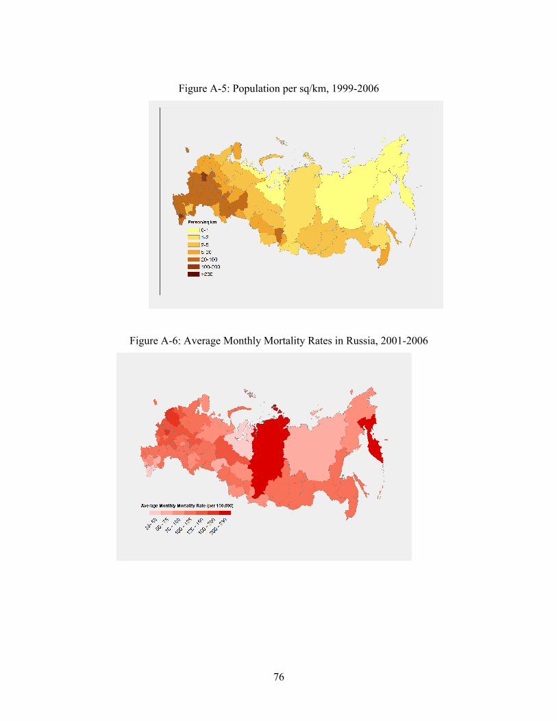
76
Figure A-5: Population per sq/km, 1999-2006
Figure A-6: Average Monthly Mortality Rates in Russia, 2001-2006

77
Figure A-7: Change in Annual Mortality in Russia (No Adaptation)
Figure A-8: Change in Annual Mortality in Russia (With Adaptation)

78
Figure A-9: Increase in Winter Temperature (USA, 2070-2099)
Figure A-10: Increase in Summer Temperature (USA, 2070-2099)

79
B. Data Individual data come the 5% IPUMS of the 2000 Census. I dropped individuals
for whom it was not possible to identify the Metropolitan Statistical Area (MSA) of
residence in 2000 and in 1995. I also keep household heads ages 25-60.
I do not include part time workers in the sample. I define full time workers as
those who work at least 30 hours per week and more than 30 weeks per year. I compute
hourly wage as yearly wage divided by number of hours worked and dropped individuals
whose hourly wage is greater than 130 dollar per hour.
Predicting Wage
I impute the wage that the individual could earn in every location with a series of
location specific regressions of the wage on individual characteristics (Zi,j):
- five indicators of educational attainment;
- age, age squared
- six indicators of industry at the one digit level (1950 classification);
- eleven indicators of employment at the one digit level (1950
classification);
- three race indicators (white, black, and others);
- two indicators for marital status (married and single);
I also predict wage separately for female and male.

80
Geology Data
Geology Data come from USGS. I use two variables in this analysis. . Type of a
bedrock structure: sedimentary vs volcanic rock and depth to bedrock. Files are obtained
as a boundary files and were merge using GIS software to county and MSA level
shapefiles of the US. The bedrock structure instrument is calculated as a dummy variable
whether a given location (MSA) has a county, which is completely covered by non-
sedimentary rock. The depth to bedrock is the average depth across location (MSA or non
MSA area of each state).
C. Additional Robustness checks
C.1 Different Specification for Moving Costs
Now I consider a different specification for moving cost function:
€
f (di, j ) = γ1d1i, j +γ 2d2i, j ,
where d1 is a dummy variable which is equal to 1 if a person would have to move less
than 500 miles to get to location j and 0 otherwise, d2=1 if a person would have to move
more than 1000 miles to be in location j and 0 otherwise. The results of the estimation are
presented below. Estimated effects are similar to the main specification.
In the first step I estimate how wages, moving costs, marital status and number of
children affect individual’s decision to move. Marital status and number of children
determine whether an individual will be a potential mover or not, and potential movers
select a particular location according to their wages in that location, moving costs, and
other location specific factors, represented by location fixed effects.

81
As in the main specification wage has positive effect on probability to move. The
effects are larger for more educated people and younger individuals. Moving costs also as
in the main specification have the negative effect on probability to move, and these
effects are larger the father away the person would have to travel.
Marital status as before has a positive effect on a probability to be a potential
mover, except for the youngest groups. Number of children also has the expected
negative sign, suggesting that individuals with more children are less likely to be
potential movers.
Results from the second step of the estimation procedure are also similar to the
man specification. People do not like to live in locations with extremely low and high
temperatures. Older individuals are more responsive to temperature that younger
individuals. People do not like rain; prefer to live on a coast. Coefficients on density are
negative and similar in magnitude to the main specification, suggesting that people try to
avoid densely populated places.

82
Table C-1: First Step Parameter Estimates: College Graduates by Age
College Grads College Grads College Grads College Grads VARIABLES 20-30 30-40 40-55 55-65 ln(wage) 2.708 2.527 2.024 1.337 (0.0051) (0.0047) (0.006) (0.0341) <500 miles -1.416 -1.588 -1.417 -1.3831 (0.0006) (0.0005) (0.0007) (0.004) >1000 miles -0.202 -0.231 -0.226 -0.179 (0.0003) (0.0003) (0.0004) (0.0021) Married -0.218 0.166 0.320 0.237 (0.0002) (0.0002) (0.0002) (0.0009) Nchildren -0.257 -0.080 -0.085 -0.225 (0.0001) (0.0001) (0.0001) (0.0006) Observation 111653 149502 125935 21378 Notes: Standard errors in parentheses; MSA fixed effects are included but not reported; log(wage) is log of hourly wage of household head;
Table C-2: First Step Parameter Estimates: Some College by Age
Some College Some College Some College Some College VARIABLES 20-30 30-40 40-55 55-65 ln(wage) 1.331 1.757 1.765 1.526 (0.0078) (0.0082) (0.0092) (0.0601) <500 miles -1.145 -1.396 -1.246 -1.327 (0.0012) (0.001) (0.0012) (0.0078) >1000 miles -0.069 -0.187 -0.138 -0.052 (0.0005) (0.0005) (0.0006) (0.0039) Married -0.105 0.144 0.250 0.274 (0.0002) (0.0002) (0.0002) (0.0013) Nchildren -0.149 -0.059 -0.115 -0.232 (0.0001) (0.0001) (0.0001) (0.001) Observation 99578 105210 94677 14582 Notes: Standard errors in parentheses; MSA fixed effects are included but not reported; log(wage) is log of hourly wage of household head;

83
Table C-3: First Step Parameter Estimates: High School by Age
Some College Some College Some College Some College VARIABLES 20-30 30-40 40-55 55-65 ln(wage) 0.4107 0.5075 0.4345 0.7124 (0.0054) (0.0051) (0.006) (0.0262) <500 miles -0.9991 -1.2249 -1.1303 -1.1066 (0.001) (0.0008) (0.001) (0.0044) >1000 niles 0.0087 -0.0666 -0.0412 -0.0533 (0.0004) (0.0004) (0.0005) (0.0021) Married -0.0094 0.0992 0.2055 0.2645 (0.0001) (0.0001) (0.0002) (0.0007) Nchildren -0.0852 -0.0413 -0.0803 -0.1421 (0.0001) (0.0001) (0.0001) (0.0003) Observation 162554 179450 154826 32684 Notes: Standard errors in parentheses; MSA fixed effects are included but not reported; log(wage) is log of hourly wage of household head;

84
Table C-4: Second Step Parameter Estimates: College Grads by Age
IV Estimates of the Effects of Climate Variables
College Grads
College Grads
College Grads
College Grads
VARIABLES 20-30 30-40 40-55 55-65 # days with with av. temp <200F -0.017 -0.018* -0.021** -0.022** (0.011) (0.011) (0.011) (0.011) # days with with av. temp in [200F; 400F] -0.004 -0.002 -0.002 -0.003 (0.005) (0.005) (0.005) (0.005) # days with with av. temp in [400F; 600F] -0.007 -0.006 -0.006 -0.008 (0.006) (0.006) (0.006) (0.005) # days with with av. temp in [600F; 800F] - - - - # days with with av. temp >800F -0.009 -0.007 -0.006 -0.008 (0.009) (0.009) (0.008) (0.008) Annual rainfall <25 in -0.326 -0.048 0.083 0.372 (0.517) (0.505) (0.481) (0.480) Annual rainfall in [25in; 45in] - - - - Annual rainfall > 45in -0.850** -0.693* -0.657* -0.501 (0.389) (0.388) (0.372) (0.390) Coast 0.341 0.475** 0.553*** 0.574*** (0.223) (0.218) (0.206) (0.211) Log(dens) -0.353 -0.341 -0.340 -0.251 (0.273) (0.268) (0.252) (0.250) Observations 328 328 328 328 Underident rk LM stat 14.54 14.54 14.54 14.54 Weak Cragg-Donald Wald F 15.20 15.20 15.20 15.20 Notes: IV estimates using bedrock structure as an instrument; Robust standard errors in parentheses. *** p<0.01, ** p<0.05, * p<0.11
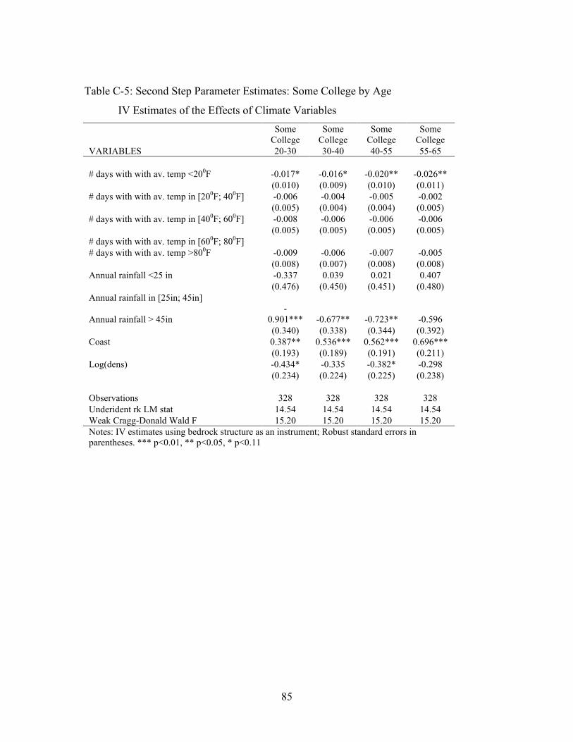
85
Table C-5: Second Step Parameter Estimates: Some College by Age
IV Estimates of the Effects of Climate Variables
Some
College Some
College Some
College Some
College VARIABLES 20-30 30-40 40-55 55-65 # days with with av. temp <200F -0.017* -0.016* -0.020** -0.026** (0.010) (0.009) (0.010) (0.011) # days with with av. temp in [200F; 400F] -0.006 -0.004 -0.005 -0.002 (0.005) (0.004) (0.004) (0.005) # days with with av. temp in [400F; 600F] -0.008 -0.006 -0.006 -0.006 (0.005) (0.005) (0.005) (0.005) # days with with av. temp in [600F; 800F] # days with with av. temp >800F -0.009 -0.006 -0.007 -0.005 (0.008) (0.007) (0.008) (0.008) Annual rainfall <25 in -0.337 0.039 0.021 0.407 (0.476) (0.450) (0.451) (0.480) Annual rainfall in [25in; 45in]
Annual rainfall > 45in -
0.901*** -0.677** -0.723** -0.596 (0.340) (0.338) (0.344) (0.392) Coast 0.387** 0.536*** 0.562*** 0.696*** (0.193) (0.189) (0.191) (0.211) Log(dens) -0.434* -0.335 -0.382* -0.298 (0.234) (0.224) (0.225) (0.238) Observations 328 328 328 328 Underident rk LM stat 14.54 14.54 14.54 14.54 Weak Cragg-Donald Wald F 15.20 15.20 15.20 15.20 Notes: IV estimates using bedrock structure as an instrument; Robust standard errors in parentheses. *** p<0.01, ** p<0.05, * p<0.11

86
Table C-6: Second Step Parameter Estimates: Hight School by Age
IV Estimates of the Effects of Climate Variables
High
School High
School High
School High
School VARIABLES 20-30 30-40 40-55 55-65
# days with with av. temp <200F -
0.030*** -
0.025*** -0.030*** -0.027*** (0.009) (0.009) (0.010) (0.010) # days with with av. temp in [200F; 400F] -0.002 -0.001 -0.001 -0.002 (0.005) (0.004) (0.005) (0.005) # days with with av. temp in [400F; 600F] -0.009* -0.008 -0.009* -0.010** (0.005) (0.005) (0.005) (0.005) # days with with av. temp in [600F; 800F] # days with with av. temp >800F -0.009 -0.007 -0.009 -0.008 (0.008) (0.007) (0.008) (0.008) Annual rainfall <25 in -0.352 -0.063 -0.238 -0.095 (0.461) (0.437) (0.463) (0.464) Annual rainfall in [25in; 45in]
Annual rainfall > 45in -
0.954*** -0.779** -0.835** -0.674* (0.331) (0.327) (0.346) (0.359) Coast 0.566*** 0.620*** 0.678*** 0.602*** (0.189) (0.186) (0.195) (0.196) Log(dens) -0.407* -0.290 -0.385* -0.339 (0.225) (0.218) (0.230) (0.231) Observations 328 328 328 328 Underident rk LM stat 14.54 14.54 14.54 14.54 Weak Cragg-Donald Wald F 15.20 15.20 15.20 15.20 Notes: IV estimates using bedrock structure as an instrument; Robust standard errors in parentheses. *** p<0.01, ** p<0.05, * p<0.11
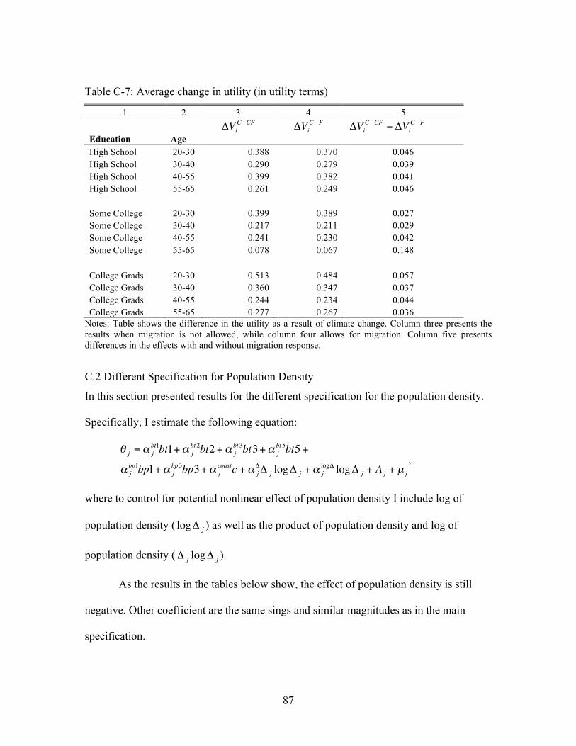
87
Table C-7: Average change in utility (in utility terms)
1 2 3 4 5
Education Age
€
ΔViC −CF
€
ΔViC −F
€
ΔViC −CF − ΔVi
C −F
High School 20-30 0.388 0.370 0.046 High School 30-40 0.290 0.279 0.039 High School 40-55 0.399 0.382 0.041 High School 55-65 0.261 0.249 0.046 Some College 20-30 0.399 0.389 0.027 Some College 30-40 0.217 0.211 0.029 Some College 40-55 0.241 0.230 0.042 Some College 55-65 0.078 0.067 0.148 College Grads 20-30 0.513 0.484 0.057 College Grads 30-40 0.360 0.347 0.037 College Grads 40-55 0.244 0.234 0.044 College Grads 55-65 0.277 0.267 0.036
Notes: Table shows the difference in the utility as a result of climate change. Column three presents the results when migration is not allowed, while column four allows for migration. Column five presents differences in the effects with and without migration response.
C.2 Different Specification for Population Density
In this section presented results for the different specification for the population density.
Specifically, I estimate the following equation:
€
θ j = α jbt1bt1+α j
bt 2bt2 +α jbt 3bt3+α j
bt 5bt5 +
α jbp1bp1+α j
bp3bp3+α jcoastc +α j
ΔΔ j logΔ j +α jlogΔ logΔ j + A j + µ j
,
where to control for potential nonlinear effect of population density I include log of
population density (
€
logΔ j ) as well as the product of population density and log of
population density (
€
Δ j logΔ j ).
As the results in the tables below show, the effect of population density is still
negative. Other coefficient are the same sings and similar magnitudes as in the main
specification.

88
Table C-8: Second Step Parameter Estimates: College Grads by Age Groups:
IV Estimates of the Effects of Climate Variables
20-30 30-40 40-55 55-65
VARIABLES College Grads
College Grads
College Grads
College Grads
# days with with av. temp <200F -0.042* -0.047* -0.052** -0.054** (0.025) (0.026) (0.026) (0.025) # days with with av. temp in [200F; 400F] -0.015 -0.013 -0.013 -0.015 (0.012) (0.013) (0.013) (0.013) # days with with av. temp in [400F; 600F] -0.015 -0.017 -0.018 -0.020* (0.012) (0.013) (0.012) (0.012) # days with with av. temp in [600F; 800F] - - - - # days with with av. temp >800F -0.023 -0.022 -0.022 -0.025 (0.015) (0.016) (0.016) (0.016) Annual rainfall <25 in -2.251** -2.327** -2.293** -2.205** (0.979) (1.056) (1.044) (1.038) Annual rainfall in [25in; 45in] - - - - Annual rainfall > 45in -2.131** -2.160** -2.155** -1.963** (0.877) (0.937) (0.915) (0.911) Coast 0.355 0.487* 0.539** 0.566** (0.250) (0.263) (0.255) (0.255) Log(dens) -1.346** -1.496** -1.538** -1.511** (0.643) (0.700) (0.688) (0.673) Dens*Log(dens) 0.014** 0.015** 0.015** 0.016** (0.006) (0.006) (0.006) (0.006) Observations 328 328 328 328 Underident rk LM stat 7.171 Notes: IV estimates using bedrock structure and depth to bedrock as an instruments; Coast variable, district division dummies and a constant are included, but not reporter; Robust standard errors in parentheses. *** p<0.01, ** p<0.05, * p<0.1

89
Table C-9: Second Step Parameter Estimates: Some College by Age Groups
IV Estimates of the Effects of Climate Variables
20-30 30-40 40-55 55-65
VARIABLES Some
College Some
College Some
College Some
College # days with with av. Temp <200F -0.031 -0.034* -0.043* -0.047** (0.020) (0.021) (0.023) (0.023) # days with with av. Temp in [200F; 400F] -0.008 -0.007 -0.010 -0.008 (0.010) (0.010) (0.011) (0.011) # days with with av. Temp in [400F; 600F] -0.012 -0.013 -0.016 -0.017 (0.010) (0.010) (0.011) (0.011) # days with with av. Temp in [600F; 800F] - - - - # days with with av. Temp >800F -0.016 -0.014 -0.017 -0.016 (0.013) (0.013) (0.015) (0.015) Annual rainfall <25 in -1.612** -1.596* -1.937** -1.764* (0.809) (0.831) (0.940) (0.936) Annual rainfall in [25in; 45in] - - - - Annual rainfall > 45in -1.467** -1.566** -1.794** -1.758** (0.706) (0.733) (0.818) (0.837) Coast 0.330* 0.488** 0.510** 0.688*** (0.199) (0.207) (0.228) (0.240) Log(dens) -1.117** -1.174** -1.413** -1.337** (0.519) (0.544) (0.609) (0.612) Dens*log(dens) 0.011** 0.012** 0.014** 0.014** (0.005) (0.005) (0.006) (0.006) Observations 328 328 328 328 Underident rk LM stat 7.171 Notes: IV estimates using bedrock structure and depth to bedrock as an instruments; Coast variable, district division dummies and a constant are included, but not reporter; Robust standard errors in parentheses. *** p<0.01, ** p<0.05, * p<0.1

90
Table C-10: Second Step Parameter Estimates: High School by Age Groups
IV Estimates of the Effects of Climate Variables
20-30 30-40 40-55 55-65
VARIABLES High
School High
School High
School High
School # days with with av. temp <200F -0.041** -0.042** -0.048** -0.049** (0.019) (0.021) (0.022) (0.023) # days with with av. temp in [200F; 400F] -0.004 -0.005 -0.007 -0.008 (0.009) (0.010) (0.010) (0.011) # days with with av. temp in [400F; 600F] -0.014 -0.015 -0.016 -0.019* (0.010) (0.010) (0.011) (0.011) # days with with av. temp in [600F; 800F] - - - - # days with with av. temp >800F -0.014 -0.015 -0.016 -0.017 (0.012) (0.013) (0.014) (0.014) Annual rainfall <25 in -1.420* -1.499* -1.689* -1.865** (0.756) (0.816) (0.882) (0.914) Annual rainfall in [25in; 45in] - - - - Annual rainfall > 45in -1.382** -1.562** -1.639** -1.645** (0.675) (0.732) (0.788) (0.820) Coast 0.466** 0.527** 0.566** 0.517** (0.196) (0.209) (0.223) (0.230) Log(dens) -1.109** -1.202** -1.354** -1.421** (0.498) (0.543) (0.581) (0.601) Dens*log(dens) 0.011** 0.013** 0.014** 0.015** (0.005) (0.005) (0.006) (0.006) Observations 328 328 328 328 Underident rk LM stat 7.171 Notes: IV estimates using bedrock structure and depth to bedrock as an instruments; Coast variable, district division dummies and a constant are included, but not reporter; Robust standard errors in parentheses. *** p<0.01, ** p<0.05, * p<0.1

91
REFERENCES
Albouy, D., Graf W., Kellogg R., and H. Wolff. (2011): “Climate Amenities, Climate Change and American Quality of Life”, Unpublished paper.
Barreca, A., (2012): “Climate Change, Humidity, and Mortality in the United States”, Journal of Environmental Economics and Management, 63(1): 19-34
Barreca, A., Karen C., Deschênes O., Greenstone M., and J. S. Shapiro. (2013): “Adapting to climate change the remarkable decline in the U.S. temperature-mortality relationship over the 20th century”, NBER Working Paper 18692 http://www.nber.org/papers/w18692
Basu, R., and J. M. Samet. (2002): “Relation Between Elevated Ambient Temperature and Mortality: A Review of the Epidemiologic Evidence”, Epidemiologic Review. 24 (December): 190-202.
Bayer, P., Keohane N., and C. Timmins. (2009): “Migration and Hedonic Valuation: The Case of Air Quality”, Journal of Environmental Economics and Management 58: 1–14.
Bayer, P,. and C. Timmins. (2005): “On the Equilibrium Properties of Locational Sorting Models,” Journal of Urban Economics, 57, 462–477.
Bayer, P,. and C. Timmins. (2007): “Estimating Equilibrium Models of Sorting across Locations”, The Economic Journal 117(518): 353–374.
Berry, S., Levinsohn J., and A. Pakes. (1995): “Automobile Prices in Market Equilibrium”, Econometrica 63(4): 841–890.
Blomquist, G.C., Berger M.C., and J.P. Hoehn. (1988): “New Estimates of Quality of Life in Urban Areas”, American Economic Review 78(1): 89–107.
Bresnahan T., (1981): “Departures from Marginal-Cost Pricing in the American Automobile Industry,” Journal of Econometrics, 17, 201–227.
Burgess, R., Deschênes O., Donaldson D., and M. Greenstone. (2011): "Weather and Death in India: Mechanisms and Implications for Climate Change," Mimeograph, MIT Department of Economics.
Cragg, M., and M. Kahn. (1997): “New Estimates of Climate Demand: Evidence from Location Choice”, Journal of Urban Economics 42: 261–284.
Cragg, M., and M. Kahn. (1999): “Climate Consumption and Climate Pricing from 1940 to 1990”, Regional Science and Urban Economics 29: 519–539.
92
Deschênes, O., and M. Greenstone. (2011): “Climate Change, Mortality, and Adaptation: Evidence from Annual Fluctuations in Weather in the US”, American Economic Journal: Applied Economics 3(4): 152–185.
Deschênes, O., and M. Greenstone. (2007): “The Economic Impacts of Climate Change: Evidence from Agricultural Profits and Random Fluctuations in Weather”, American Economic Review, 97 (March): 354-385.
Deschênes, O,. and M. Greenstone. (2011): “Climate change, mortality, and adaptation: evidence from annual fluctuation in weather in the US”, American Economic Journal: Applied Economics, 3(4): 152–85.
Deschênes, O., and M., Enrico. (2009): “Extreme Weather Events, Mortality and Migration”, Review of Economics and Statistics, 91(4): 659-681
Gyourko, J., and J. Tracy. (1991): “The Structure of Local Public Finance and the Quality of Life”, Journal of Political Economy 99(4): 774–806.
Joshua Graff, Z., , and M. J. Neidell. (2010): “Temperature and the allocation of time: Implication for climate change”, NBER Working Paper 15717.
Mityakov, S., and T. Mroz. (2014): “Economic Theory as a Guide for the Specification and Interpretation of Empirical Household Production Functions”, Clemson University mimeo
Roback, J., (1982): “Wages, Rents, and the Quality of Life”, Journal of Political Economy, 90(6), 1257–1278.
Rosenthal, S. and S., William. (2008): "The attenuation of human capital spillovers," Journal of Urban Economics, Elsevier, vol. 64(2), pages 373-389, September
Sinha, P., and M. Cropper. (2013): “The Value of Climate Amenities: Evidence from US Migration Decisions”, NBER Working Paper No. 18756
Smith, V.K. (1983): “The Role of Site and Job Characteristics in Hedonic Wage Models”, Journal of Urban Economics 13(3): 296–321.
Stern, N. (2007) “The Economics of Climate Change – The Stern Review”, Cambridge: Cambridge University Press
Timmins, C. (2007): “ If you cannot take the heat, get out of the cerrado... Recovering the equilibrium amenity cost of nonmarginal climate change in Brazil”, Journal of Regional Science. 47(1): 1-25.
British Atmospheric Data Centre. 2007. “Hadley Climate Model 3.” http://badc.nerc.ac.uk/data/.

93
The Hadley Climate Model 3 (HadCM3) data from the British Atmospheric Data Centre (http://badc.nerc.ac.uk/home/)
Mortality, GDP and Population data from Russian Federal State Statistics Service (http://gks.ru)
Temperature Data from National Climatic Data Center (http://www.nodc.noaa.gov)
The National Center for Atmospheric Research’s (NCAR) Community Climate System Model 3(CCSM 3). (https://esg.llnl.gov:8443/index.jsp )