Essays on Antitrust Issues for Horizontal and Vertical Mergers · Essays on Antitrust Issues for Horizontal and ... O segundo ensaio utiliza um modelo semelhante ao caracterizado

Essays on Antitrust Issues for Horizontal andVertical Mergers

Mariana Alves da Cunha

Tese de Doutoramento em Economia

Orientada por:

Professor Doutor Helder Vasconcelos

Professora Doutora Paula Sarmento

Porto, Dezembro 2014

For my grandfather (in memoriam).

Biographical Note

Mariana Alves da Cunha was born on October 18, 1987, in Porto, Portugal.

She concluded her undergraduate studies in Economics in 2008 and Master studies in

Economics in 2010, both from Faculdade de Economia e Gestao, Universidade Catolica -

Centro Regional do Porto. Her Master’s dissertation entitled “Eficiencia do Sector de Energia

Electrica na Uniao Europeia” has been supervised by Professor Carlos Santos.

During her Master studies, Mariana has taught at Universidade Catolica - Centro Regional

do Porto (2008-2010): Microeconomics, Econometrics and Mathematics.

In September of 2010, she started her PhD in Economics at Faculdade de Economia da

Universidade do Porto, under the supervision of Professors Helder Vasconcelos and Paula

Sarmento. Her most recent research on mergers has been presented in conferences, as the

4th and 5th edition UECE Lisbon Meetings: Game Theory and Applications (both in Lisbon,

Portugal) and the 8th Annual Meeting of the Portuguese Economic Journal (Braga, Portugal).

Her research has also resulted in two publications in the Journal of Industry Competition in

Trade.

i

Acknowledgements

During my PhD thesis, I received support from many people. I am gratefull to them all.

First of all, I would like to express my gratitude to my supervisors Helder Vasconcelos

and Paula Sarmento from whom I have learned a lot in many ways along this journey. This

work would not be possible without their continuous support, encouragement and guidance.

Their incentives certainly made me go further and I deeply thank them for the patient and for

being present whenever I needed help.

I am also grateful to all of those who have comment some of the essays in this thesis at

conferences and seminars. I would like to highlight the valuable suggestions and comments

of Professors Antonio Brandao, Helder Valente, Joana Pinho, Joao Correia da Silva, Ricardo

Ribeiro and Sofia Castro Gothen.

I gratefully acknowledge FCT (Fundacao para a Ciencia e Tecnologia) for financial sup-

port through a doctoral grant reference SFRH/BD/70000/2010.

I am indebted to a number of friends that have made my PhD a more pleasant experience:

Rita, Miriam, Vera, Diogo, Filipe and Tiago.

Finally, a word of gratitude goes to my boyfriend, Nuno, and to my parents and brother,

for all their unconditional support, love and (huge) patience, during all these years.

Mariana Cunha, Porto, 2014.

ii

Resumo

A presente tese inclui quatro ensaios sobre questoes de polıtica de concorrencia na analise de

fusoes horizontais e verticais. No primeiro ensaio estudamos fusoes horizontais quando as

empresas tem comportamentos estrategicos assimetricos. Alem disso, analisamos uma fusao

sequencial num cenario onde: (i) as empresas concorrem a Stackelberg; (ii) inicialmente

as empresas sao simetricas, mas as fusoes podem dar origem a ganhos de eficiencia e, por

consequencia, a assimetrias de custos entre as empresas; e (iii) todas as fusoes tem de ser

submetidas a aprovacao pela Autoridade da Concorrencia. Em particular, consideramos dois

tipos de Autoridades da Concorrencia: uma Autoridade da Concorrencia mıope, que avalia

a proposta de fusao sem antecipar que poderao existir outras fusoes subsequentes, e uma

Autoridade da Concorrencia com visao futura, que antecipa a estrutura final de mercado, no

caso da primeira fusao ser aprovada.

O segundo ensaio utiliza um modelo semelhante ao caracterizado no primeiro ensaio.

Neste ensaio estudamos a lucratividade das fusoes, o problema do free-riding e os efeitos in-

duzidos das fusoes no bem estar social e no bem estar dos consumidores, quando as empresas

concorrem a Stackelberg e as fusoes geram assimetrias de custos entre as empresas existentes

na industria. Em particular, mostramos que as conclusoes sobre a lucratividade das fusoes,

os efeitos no bem estar e a existencia do problema do free-ridding depende de forma crucial

dos ganhos de eficiencia gerados pelas fusoes.

No terceiro ensaio exploramos o papel da incerteza na decisao de fusao e no seu controlo

pelas autoridades de concorrencia. Num cenario de concorrencia a Cournot, consideramos

que as fusoes podem gerar ganhos de eficiencia incertos e que todas a fusoes tem de ser

iii

submetidas para aprovacao da Autoridade da Concorrencia. O objectivo deste ensaio e nao

so estudar o impacto da incerteza na probabilidade da fusao ser proposta pelas empresas

e aceite pela Autoridade da Concorrencia mas tambem analisar de que forma a incerteza

influencia os incentivos das empresas que ficam de fora da fusao a prosseguirem estrategias

de free-riding.

Por fim, no quarto ensaio analisamos de que forma a integracao vertical aumenta os in-

centivos ao conluio das empresas retalhistas. O principal contributo deste ensaio e realcar a

relacao entre dois tipos de estrategias das empresas: a integracao vertical e o conluio, num

cenario em que nem todas as empresas aceitam o acordo colusivo (conluio incompleto).

iv

Abstract

This thesis comprises four essays on antitrust issues for horizontal and vertical mergers. In

the first essay we study horizontal mergers when firms have asymmetric strategic roles. In this

essay we assume a sequential merger formation game in a setting where: (i) firms compete a

la Stackelberg; (ii) all firms are ex-ante symmetric, but as mergers may give rise to endoge-

nous efficiency gains, cost asymmetries between the remaining firms in the industry may be

created; and (iii) every merger has to be submitted for approval to the Antitrust Authority. In

particular, we consider two possible types of Antitrust Authorities: a myopic Antitrust Au-

thority, that evaluates a merger proposal without anticipating possible subsequent mergers,

and a forward looking Antitrust Authority, which is able to anticipate the ultimate market

structure if the merger is approved.

The second essay uses a framework similar to the previous one. In this essay we inves-

tigate mergers’ profitability, free-riding problem and induced effects on social and consumer

welfare when firms are in a Stackelberg market and mergers can create cost heterogeneity

between the remaining firms in the industry. In particular, we show that conclusions about

the merger profitability, the social welfare effects and the existence of a free-riding problem

crucially depend on whether the merger creates synergies.

In the third essay we explore the role of uncertainty in merger control and in merger de-

cisions. In a Cournot setting, we consider that mergers may give rise to uncertain efficiency

gains and that every merger has to be submitted for approval to the Antitrust Authority. We

assume that both the Antitrust Authority and the firms in the industry face the same uncer-

tainty about the future efficiency gains induced by the merger. The purpose of this essay is

v

not only to study the impact of the existence of uncertainty in the likelihood of the merger

being proposed by the firms and accepted by the Antitrust Authority but also to analyze how

the uncertainty affects outsider firms’ incentives to free-ride on it.

Finally, the fourth essay analyzes how vertical integration increases downstream firm’s

incentives to collude. The main contribution of this essay is to highlight the importance of

considering, simultaneously, two types of firms’ strategies: vertical integration and collusion,

in a context where some firms have no incentives to collude (incomplete collusion).

vi

Contents

1 Introduction 1

2 Efficiency gains of mergers in Stackelberg markets with an active Antitrust Au-

thority 5

2.1 Introduction . . . . . . . . . . . . . . . . . . . . . . . . . . . . . . . . . . . 5

2.2 Basic Model . . . . . . . . . . . . . . . . . . . . . . . . . . . . . . . . . . . 10

2.3 Before the merger . . . . . . . . . . . . . . . . . . . . . . . . . . . . . . . . 12

2.4 Merger involving the two leader firms . . . . . . . . . . . . . . . . . . . . . 13

2.4.1 Merger of two leaders under a Myopic AA . . . . . . . . . . . . . . 14

2.4.2 Merger of two leader firms under a forward looking AA . . . . . . . 19

2.5 Extensions . . . . . . . . . . . . . . . . . . . . . . . . . . . . . . . . . . . . 24

2.5.1 Social Welfare standard . . . . . . . . . . . . . . . . . . . . . . . . 24

2.5.2 Other merger possibilities . . . . . . . . . . . . . . . . . . . . . . . 26

2.6 Conclusion . . . . . . . . . . . . . . . . . . . . . . . . . . . . . . . . . . . 30

Appendix . . . . . . . . . . . . . . . . . . . . . . . . . . . . . . . . . . . . . . . 33

3 Mergers in Stackelberg Markets with Efficiency Gains 37

3.1 Introduction . . . . . . . . . . . . . . . . . . . . . . . . . . . . . . . . . . . 37

3.2 Baseline Model . . . . . . . . . . . . . . . . . . . . . . . . . . . . . . . . . 39

3.2.1 Pre-merger equilibrium . . . . . . . . . . . . . . . . . . . . . . . . . 41

3.3 Merger Effects . . . . . . . . . . . . . . . . . . . . . . . . . . . . . . . . . 42

3.3.1 Insiders’ Profitability . . . . . . . . . . . . . . . . . . . . . . . . . . 44

vii

3.3.1.1 Numerical simulation results on merger profitability . . . . 49

3.3.2 Free-riding problem . . . . . . . . . . . . . . . . . . . . . . . . . . 51

3.3.3 Consumer Surplus and Social Welfare . . . . . . . . . . . . . . . . . 53

3.3.3.1 Consumer Surplus Standard . . . . . . . . . . . . . . . . . 54

3.3.3.2 Social Welfare Standard . . . . . . . . . . . . . . . . . . . 57

3.4 Simulation Results . . . . . . . . . . . . . . . . . . . . . . . . . . . . . . . 58

3.5 Conclusion . . . . . . . . . . . . . . . . . . . . . . . . . . . . . . . . . . . 63

Appendix . . . . . . . . . . . . . . . . . . . . . . . . . . . . . . . . . . . . . . . 64

4 Uncertain Efficiency Gains and Merger Policy 81

4.1 Introduction . . . . . . . . . . . . . . . . . . . . . . . . . . . . . . . . . . . 81

4.2 Basic Framework . . . . . . . . . . . . . . . . . . . . . . . . . . . . . . . . 85

4.3 Pre-Merger equilibrium . . . . . . . . . . . . . . . . . . . . . . . . . . . . . 86

4.4 Merger Analysis . . . . . . . . . . . . . . . . . . . . . . . . . . . . . . . . . 86

4.4.1 Product Market Competition . . . . . . . . . . . . . . . . . . . . . . 89

4.4.2 Expected Profits and Consumer Surplus . . . . . . . . . . . . . . . . 90

4.4.3 Antitrust Authority’s Decision . . . . . . . . . . . . . . . . . . . . . 94

4.4.4 Merger Decision . . . . . . . . . . . . . . . . . . . . . . . . . . . . 95

4.4.5 Free-riding Problem . . . . . . . . . . . . . . . . . . . . . . . . . . 96

4.5 Numerical Application . . . . . . . . . . . . . . . . . . . . . . . . . . . . . 98

4.6 Concluding Remarks . . . . . . . . . . . . . . . . . . . . . . . . . . . . . . 103

Appendix . . . . . . . . . . . . . . . . . . . . . . . . . . . . . . . . . . . . . . . 104

5 Does Vertical Integration Promote Downstream Incomplete Collusion? An Eval-

uation of Static and Dynamic Stability 113

5.1 Introduction . . . . . . . . . . . . . . . . . . . . . . . . . . . . . . . . . . . 113

5.2 The Baseline Model . . . . . . . . . . . . . . . . . . . . . . . . . . . . . . . 118

5.2.1 The Model without Vertical Integration . . . . . . . . . . . . . . . . 122

5.2.1.1 Collusive Results . . . . . . . . . . . . . . . . . . . . . . 122

5.2.1.2 Cournot Equilibrium . . . . . . . . . . . . . . . . . . . . 124

viii

5.2.1.3 Deviation Results . . . . . . . . . . . . . . . . . . . . . . 125

5.2.2 The Model of Vertical Integration with a cartel member . . . . . . . . 127


5.2.2.2 Cournot equilibrium . . . . . . . . . . . . . . . . . . . . . 130


5.2.3 The Model of Vertical Integration with a fringe firm . . . . . . . . . 134


5.2.3.2 Cournot equilibrium . . . . . . . . . . . . . . . . . . . . . 136


5.3 Welfare analysis . . . . . . . . . . . . . . . . . . . . . . . . . . . . . . . . . 137

5.4 Discussion of Results . . . . . . . . . . . . . . . . . . . . . . . . . . . . . . 140

5.5 Concluding Remarks . . . . . . . . . . . . . . . . . . . . . . . . . . . . . . 144

Appendix . . . . . . . . . . . . . . . . . . . . . . . . . . . . . . . . . . . . . . . 146

References 155

ix

List of Figures

2.1 Merger of two leaders: equilibrium outcomes with a myopic AA. . . . . . . . 18

2.2 Merger of two leaders: equilibrium outcomes with a forward looking AA. . . 23

2.3 Merger of two leaders: equilibrium results with a myopic SW-maximizer AA. 24

2.4 Merger of two leaders: equilibrium results with a forward-looking SW-maximizer

AA. . . . . . . . . . . . . . . . . . . . . . . . . . . . . . . . . . . . . . . . 25

2.5 Merger of two followers: equilibrium outcomes with a myopic AA. . . . . . 27

2.6 Merger of two followers: equilibrium outcomes with a forward looking AA. . 27

2.7 Merger of one leader and one follower: equilibrium results with a myopic AA. 28

2.8 Merger of one leader and one follower: equilibrium results with a forward

looking AA. . . . . . . . . . . . . . . . . . . . . . . . . . . . . . . . . . . . 29

3.1 Merger profitability for n = 6 and m = 3 . . . . . . . . . . . . . . . . . . . 47

3.2 ∆Consumer Surplus . . . . . . . . . . . . . . . . . . . . . . . . . . . . . . 55

3.3 Critical parameters of α for a merger between two leader firms . . . . . . . . 78

3.4 Critical parameters of α for a merger between two follower firms . . . . . . . 79

3.5 Critical parameters of α for a merger between a leader and a follower firms . 80

4.1 AA’s decision (m = 2) . . . . . . . . . . . . . . . . . . . . . . . . . . . . . 99

4.2 AA’s decision (m = 3) . . . . . . . . . . . . . . . . . . . . . . . . . . . . . 100

4.3 AA’s decision (m = 4) . . . . . . . . . . . . . . . . . . . . . . . . . . . . . 101

4.4 AA’s decision (m = 2, 3, 4) . . . . . . . . . . . . . . . . . . . . . . . . . . 102

5.1 Model’s critical discount values for K=F+2 . . . . . . . . . . . . . . . . . . 141

x

5.2 Model’s critical discount values for K=F+3 . . . . . . . . . . . . . . . . . . 141

xi

List of Tables

2.1 Efficiency gains results, by region and by AA for each merger case . . . . . 30

3.1 Efficiency gains conditions for profitable mergers and no exit . . . . . . . . . 49

3.2 Effects of a merger between two leader firms . . . . . . . . . . . . . . . . . 59

3.3 Effects of a merger between two follower firms . . . . . . . . . . . . . . . . 60

3.4 Effects of a merger between a leader and a follower firms . . . . . . . . . . . 61

5.1 Static and Dynamic Stability Results - Model 1 . . . . . . . . . . . . . . . . 126



5.4 Welfare analysis . . . . . . . . . . . . . . . . . . . . . . . . . . . . . . . . . 139

xii

Chapter 1

Introduction

The present thesis is organized in five chapters. This first chapter gives an overview of the

thesis’s organization and familiarizes the reader with the main research topics. Each research

question is answered in its own chapter as an independent essay, consisting of introduction

that includes the literature review and some practical applications, methodology, discussion

of the results, conclusion and policy implications. Some of these individual essays are, how-

ever, related to each other and some overlap in content is inevitable, especially with regard to

the assumptions of the theoretical models.

Horizontal mergers in concentrated industries are an important issue for antitrust authori-

ties. Mergers can reduce industry competition and hence result in higher prices, which could

harm consumers. However, a merger can also be welfare-enhancing if it generates efficiency

gains, increases incentives for innovation or creates synergies and scale economies among

firms. Then, the efficiency gains might offset the increased market power and result in higher

social welfare. Therefore, the horizontal merger could actually lead to more efficient firms

and to lower prices, which benefits consumers. Usually, the welfare analysis of mergers

assumes that firms have incentives to merge because this could increase their profits by in-

creasing the prices or reducing the costs. Stigler (1950) argued that firms that do not merge

(outsiders) may also benefit more than the participants (insiders). With the merger, the new

firm will reduce its production and then the industry price will increase. However, the non-

1

participants firms will expand their output and therefore will have higher profits due to the

high industry price.

The first essay (Chapter 2) is concerned with horizontal mergers, in a setting where the

firms in the market have asymmetric strategic roles. In this essay we assume a sequential

merger formation game in a setting where: (i) firms compete a la Stackelberg; (ii) all firms are

ex-ante symmetric, but mergers may give rise to endogenous efficiency gains and, therefore,

cost asymmetries between the remaining firms in the industry; and (iii) every merger has to

be submitted for approval to the Antitrust Authority. In particular, we consider two possible

types of Antitrust Authority: a myopic Antitrust Authority, that evaluates a merger proposal

without anticipating that this merger might trigger other subsequent mergers, and a forward

looking Antitrust Authority, which is able to anticipate the ultimate market structure a merger

will lead to, if approved. We find that these two types of Antitrust Authority adopt similar

decisions whenever a merger would not trigger the exit of outsider firms. The Antitrust

Authorities’ decisions are, however, shown to be very different when evaluating exit-inducing

merger proposals.

The second essay (Chapter 3) is related to the previous one and is concerned with merg-

ers’ profitability, free-riding problem and induced effects on social and consumer welfare of

mergers, when firms are in a Stackelberg market and mergers can create cost heterogeneity

between the remaining firms in the industry. We find that under certain conditions regarding

the cost benefits resulting from mergers, the so called “free-riding” problem is eliminated and

mergers are not only profitable but also welfare enhancing, even with linear costs.

The assessment of the efficiency gains resulting from a merger usually raises an informa-

tion issue for antitrust authorities. Although some mergers can actually generate significant

efficiency gains, these are usually difficult to measure and verify. In practice, it is often the

case where both the firms and the antitrust authority cannot predict exactly the post-merger

efficiency gains, implying that they are not aware of all the conditions they are going to

face after the merger. Sometimes, only after the merger firms and antitrust authorities will

understand the true level of the merger’s induced efficiency gains. For instance, some phar-

2

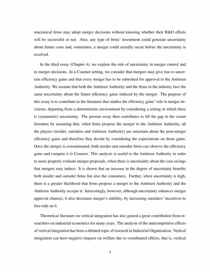
maceutical firms may adopt merger decisions without knowing whether their R&D efforts

will be successful or not. Also, any type of firms’ investment could generate uncertainty

about future costs and, sometimes, a merger could actually occur before the uncertainty is

resolved.

In the third essay (Chapter 4), we explore the role of uncertainty in merger control and

in merger decisions. In a Cournot setting, we consider that mergers may give rise to uncer-

tain efficiency gains and that every merger has to be submitted for approval to the Antitrust

Authority. We assume that both the Antitrust Authority and the firms in the industry face the

same uncertainty about the future efficiency gains induced by the merger. The purpose of

this essay is to contribute to the literature that studies the efficiency gains’ role in merger de-

cisions, departing from a deterministic environment by considering a setting in which there

is (symmetric) uncertainty. The present essay then contributes to fill the gap in the extant

literature by assuming that, when firms propose the merger to the Antitrust Authority, all

the players (insider, outsiders and Antitrust Authority) are uncertain about the post-merger

efficiency gains and therefore they decide by considering the expectations on those gains.

Once the merger is consummated, both insider and outsider firms can observe the efficiency

gains and compete a la Cournot. This analysis is useful to the Antitrust Authority in order

to more properly evaluate merger proposals, when there is uncertainty about the cost savings

that mergers may induce. It is shown that an increase in the degree of uncertainty benefits

both insider and outsider firms but also the consumers. Further, when uncertainty is high,

there is a greater likelihood that firms propose a merger to the Antitrust Authority and the

Antitrust Authority accepts it. Interestingly, however, although uncertainty enhances merger

approval chances, it also decreases merger’s stability, by increasing outsiders’ incentives to

free-ride on it.

Theoretical literature on vertical integration has also gained a great contribution from re-

searchers on industrial economics for many years. The analysis of the anticompetitive effects

of vertical integration has been a debated topic of research in Industrial Organization. Vertical

integration can have negative impacts on welfare due to coordinated effects, that is, vertical

3

integration may improve the sustainability of collusion among competing firms. Antitrust

authorities have remained concerned that vertical integration might facilitate collusion at up-

stream and downstream levels. Vertical integration facilitates collusion if, after the merger,

upstream or downstream firms are able to coordinate in a more effectively way than if they

were operating separately.

The fourth essay (Chapter 5) is about how vertical integration increases firm’s incentives

to collude. The literature suggests that there is a relationship between vertical integration

and collusion. Particularly, vertical integration might ease the collusive agreements, by sup-

porting the punishment and monitoring mechanisms and by allowing the agreement between

firms. Moreover, the models presented in the literature study if vertical integration facilitates

upstream or downstream collusion and differ mainly on the assumptions chosen. It is possible

to verify that most of these studies concluded that vertical integration facilitates collusion in

downstream or upstream level. The main contribution of the fourth essay is to highlight the

importance of considering, simultaneously, two types of firms’ strategies: vertical integra-

tion and collusion, in a context where some firms have no incentives to collude (incomplete

collusion). Then, we try to answer the following question: does vertical integration promote

incomplete collusion? This research topic could be very important for antitrust authorities be-

cause they are concerned with the impacts of vertical integration on collusion and how these

two types of strategies might affect social welfare. We find that a vertical merger between

an upstream firm and a downstream cartel or fringe firm promotes downstream collusion, un-

der certain conditions on the market size. Moreover, a welfare analysis shows that consumer

surplus increases with the vertical merger since it partially eliminates the double marginaliza-

tion problem. The results obtained could modify the formulation of policies towards vertical

mergers.

All of these questions are interesting and also bring some important insights that could

be helpful for the antitrust authorities’ intervention. In this context, all these issues seem to

be important for antitrust authorities when deciding whether or not to accept a horizontal or

vertical merger.

4

Chapter 2

Efficiency gains of mergers in

Stackelberg markets with an active

Antitrust Authority

2.1 Introduction

The large body of previous literature on the effects of horizontal mergers has argued that

Antitrust Authorities should pay particular attention to the balance between anticompetitive

price (market power) effects and pro-competitive merger related efficiency improvements

(see e.g. Williamson (1968) and Farrell and Shapiro (1990)).1

The European Commission (EC), in practice, has so far never used efficiency gains ar-

guments to clear a merger. When the merging parties use the “efficiency defence argument”

reporting that the merger would generate cost reductions, this claim usually has been dis-

missed by the EC. The EC uses the efficiency offence argument arguing that although the

merger would benefit the consumers in the short-run, in the long-run rival firms have incen-

tives to exit the industry and then the merging firm would become a monopolist, thereby

1The analysis of merger-induced efficiencies was introduced into the US Merger in 1997 (Section 4) and

into the European Merger Guidelines in 2004 (European Commission Horizontal Merger Guidelines, 2004/03,

Article 7).

5

harming consumers’ welfare. This efficiency offence argument has received some atten-

tion by economists, providing an informal discussion of efficiency offence arguments in EC

practices, such as Padilla (2002). The efficiency offence argument has also been formally

analyzed on a static and a dynamic framework (Motta, 2004; Motta and Vasconcelos, 2005).

However, to the best of our knowledge, scarce attention has been devoted to the study of

efficiency defence arguments, in contexts where merging parties have asymmetric strategic

power.

In this paper, we contribute to close this gap in the literature by studying an endogenous

merger formation game wherein: (i) merging parties compete a la Stackelberg; (ii) all firms

are ex-ante symmetric, but mergers may give rise to endogenous efficiency gains and, there-

fore, cost asymmetries between the remaining firms in the industry; and (iii) every merger

must be submitted for approval to an Antitrust Authority (AA). In particular, we consider

two possible types of AA: a myopic AA, that evaluates a merger proposal without antici-

pating that the corresponding merger might trigger other subsequent mergers, and a forward

looking AA, which is able to anticipate the ultimate market structure a merger will lead to if

approved.

Although in reality there are merger waves (or sequential mergers), usually the AAs rarely

adopt forward-looking decisions when analyzing a merger case, since it is hard to predict the

future behavior of the firms. Also AAs might make mistakes in predicting that following a

merger, outsiders might leave. However, the economic literature (eg. Motta and Vasconcelos

(2005) and Nocke and Whinston (2010)) has emphasized the need for those AAs to predict

which is the ultimate market structure, after the first merger takes place. Recently, the Centre

on Regulation in Europe (CERRE) published a dossier to the European Commission (EC)

where it includes some recommendations on the future regulatory policy in network industries

(CERRE, 2014). This report highlights that the EC and national competition authorities

should pay particular attention to the dynamic issues when investigating mergers such as,

in electronic communications and media markets and concludes that the merger policy is

currently not very good at assessing the dynamic effects of mergers, given its static focus on

prices. In this sense our paper is a theoretical contribution that suggests that when predicting

6

the possible impact of the merger, possible reactions by the outsiders (defensive mergers)

should be properly taken into account. More particularly, before concluding that a merger

will create such a more efficient merged entity that rivals would not be able to compete with

it, AAs should consider whether in the industry at hand there exists room for further mergers

allowing outsiders to attain similar efficiency levels, and/or whether the outsiders might be

able to enhance efficiency through internal growth.

Within this theoretical structure, we find that, when evaluating a two-firm merger pro-

posal, both myopic and forward-looking AAs adopt similar decisions if the proposed merger

would not trigger the exit of outsider firms in case it was approved (and no further mergers

take place). Nevertheless, their decisions are shown to be in sharp contrast when evaluating

exit-inducing merger proposals, i.e, in the region where efficiency gains and the fixed costs

are sufficiently high such that the merger would trigger the exit of outsider firms. In particu-

lar, under some circumstances, while the myopic AA blocks the merger under an efficiency

offence argument, the forward looking AA approves the very same merger proposal, since

it correctly anticipates that this merger will be followed by a subsequent defensive merger

involving the outsider firms of the first merger. This will lead to a duopoly situation wherein

even though firms have asymmetric strategic power, they end up being equally sized and

equally efficient, to the benefit of consumers.

This paper is mainly related to three strands in the extant literature. Firstly, it is related

to the literature on endogenous horizontal mergers, since we explicitly model the merger

formation process. Important references in this literature are Kamien and Zang (1990),

Gowrisankaran (1999), Faulı-Oller (2000), Horn and Persson (2001a,b), Motta and Vasconce-

los (2005), Fumagalli and Vasconcelos (2008), Fumagalli and Nilssen (2008), Banal-Estanol

et al. (2008), Vasconcelos (2010) and Nocke and Whinston (2010), to name a few.2

Secondly, our paper is also related to the previous literature that incorporates an active AA

into the merger formation game. Few studies have introduced the AA as an active player, such

as, Motta and Vasconcelos (2005), Fumagalli and Nilssen (2008), Fumagalli and Vasconcelos

2Other papers also assumed sequential game but with exogenous mergers, such as Nilssen and Søgard

(1998) and Salvo (2006).

7

(2008), Vasconcelos (2010) and Nocke and Whinston (2010).

Thirdly, this paper is also related to the branch of the literature that deals with the eco-

nomic analysis of merger control by taking into account the efficiency defence argument.

The efficiency defence argument refers to the case where the AA approves the merger if the

efficiencies caused by the merger more than compensate for the induced increase of market

power. Some papers include the AA’s efficiency defence argument when evaluating a merger

and some also analyze the role of structural remedies introduced by the AA after the merger

takes place, such as, Roller et al. (2000), Motta and Vasconcelos (2005), Fumagalli and

Nilssen (2008), Fumagalli and Vasconcelos (2008), Banal-Estanol et al. (2008), Vasconcelos

(2010) and Nocke and Whinston (2010).3

Our paper is closely related to Motta and Vasconcelos (2005)’s paper, who also studied

endogenous mergers, where each merger has to be approved by the AA. Motta and Vascon-

celos (2005) show that if the AA does not anticipate subsequent merging, such a myopic

AA could actually make wrong decisions. However, if the AA correctly anticipates that

the merger is followed by other mergers, no efficiency offence argument is justified. Like

Motta and Vasconcelos (2005), we also consider that the AA maximizes consumer welfare

and, therefore, the AA approves both mergers if consumer surplus increases (i.e. if prices

decrease).4

There are two major differences between Motta and Vasconcelos (2005) framework and

the setting used in this paper. First, Motta and Vasconcelos (2005) assume that the mergers

3The inclusion of an efficiency defence argument could bring an asymmetric information problem with

respect to the merger’s efficiency gains between the AA and the merging firms. Some papers consider the issue

of asymmetric information about merger-specific efficiencies, such as, Gonzalez (2004), Medvedev (2004),

Lagerlof and Heidhues (2005), Cosnita and Tropeano (2009), however, this analysis is far beyond the scope of

this paper.4By assuming that the AA evaluates mergers according to a consumer surplus standard this does not mean

that this is always better than the total welfare standard. However, as Lyons (2002) argued, the consumer

surplus standard is applied in most antitrust jurisdictions. Other papers also study how the AA should apply the

consumer surplus standard when challenging a merger, such as Besanko and Spulber (1993), Neven and Roller

(2005), Vasconcelos (2010), Nocke and Whinston (2010), Jovanovic and Wey (2012), among others.

8

occur under symmetric Cournot competition. In contrast, in this paper is assumed that the

mergers occur when firms have asymmetric strategic power and, therefore, it is assumed that

different types of mergers may occur in an industry characterized by Stackelberg competi-

tion.5 This assumption implies that, in the setting proposed in the current paper, when the

efficiency gains are very small (or even when there are no efficiency gains) a merger between

two firms will always be proposed because it still is profitable, which is not the case under

Cournot. When there is no strategic power advantage for any firm we obtain the well known

Salant et al. (1983) merger’s paradox: a merger between two firms with the same strategic

power that creates a firm of the same type is always unprofitable for the merging firms, unless

more than 80% of the firms in the industry merge or there are sufficiently high fixed costs.

Also, we found that in an asymmetric strategic power industry, the AA will be more severe

when blocking the mergers since the interval of efficiency gains where mergers are usually

accepted is greater under Stackelberg than under Cournot. Second, Motta and Vasconcelos

(2005) consider, under the forward looking AA, that after the defensive merger occurs, the

firms of the first and the second merger are allowed to seek a merger to a monopoly. However,

in this paper, we rule out merger to monopoly since we want to analyze the competitive effects

of merger proposals in which both at the status quo industry structure and in the merger

induced industry structure firms do have asymmetric strategic power.

Although this paper encompasses a theoretical exercise, it is also motivated by the prof-

itability of real-world mergers involving firms with asymmetric strategic power. A case in

point is the DRAM (Dynamic Random Access Memory) industry, where the leading man-

ufacturers announce their production plans in advance and manufacturers, which enter the

market later, respond by adjusting their quantity of DRAM produced. In addition, in this

specific industry, the last decades have witnessed a wave of mergers.6 Another example is

Microsoft’s dominance in software markets. In this case, although Microsoft usually makes

5See Daughety (1990), Feltovich (2001), Huck et al. (2001), Escrihuela-Villar and Faulı-Oller (2007), Hey-

wood and McGinty (2007, 2008) and Brito and Catalao–Lopes (2011) on the profitability of mergers involving

Stackelberg firms operating in a context without merger induced synergies.6For details, see Escrihuela-Villar and Faulı-Oller (2007) and the references cited therein.

9

decisions first, other smaller companies typically react to Microsoft’s actions when making

their own decisions. Obviously, these subsequent followers’ actions, in turn, affect Microsoft

(see e.g. Graham (2013)). In both examples, it seems reasonable and plausible to analyze

both firms and AA decisions when firms have asymmetric strategic power.

The remainder of the paper is organized as follows. Section 2.2 introduces the baseline

assumptions of the model. Section 2.3 presents the results before the merger. Section 2.4

analyzes the post-merger industry structure under two different scenarios regarding the be-

haviour of the AA (myopic and forward looking), for the case in which the merger involves

two leaders. In Section 2.5, we discuss two extensions of the benchmark model. In particular,

we extend the analysis by assuming that now both AAs consider the effects of the two-leader

merger on social welfare, instead of considering only the effects on consumer surplus. Fur-

ther, we also present the results obtained for alternative types of mergers. Finally, Section

2.6 concludes the paper by discussing the results obtained. All proofs and details on the

calculations are relegated to the Appendix.

2.2 Basic Model

We consider a market with N = 4 firms. We assume a two stage-game. First, all leaders

simultaneously choose their output levels. Second, all followers simultaneously choose their

output levels, after observing the leaders’ choices. We assume that there are two leaders

and two followers that compete in quantities over a linear demand P = 1 − Q, where Q =

QL +QF .

What distinguishes firms is the amount of capital they own. Hence, the cost function of a

firm which owns ki units of the industry capital and produces qi units of output is given by:

C(qi, ki, α) = αKkiqi + kif

where α ≥ 0,N=4∑i=1

ki = K = 4 and f > 0.

The total supply of capital is assumed to be fixed to the industry (and equal to K =

4 units) and ki is firm i’s capital holdings. By assuming that the total quantity of capital

10

available in the industry is fixed, we are also assuming that entry is very difficult in this

industry. This cost structure was proposed by Motta and Vasconcelos (2005). Each firm

operates with a constant marginal cost of production, but the level of its marginal cost is a

decreasing function of its capital holdings, ki. In addition, it is assumed that there exists a

plant specific fixed cost f , which has to be paid for each unit of industry’s capital owned by

the firm. This fixed cost could be, for instance, a plant specific fixed fee associated with an

energy suppliance contract. Also, at the status quo industry structure, each firm is endowed

with a single unit of capital (ki = 1), implying that all firms are symmetric in terms of costs.

However, cost asymmetries may arise as a result of a merger (or a series of mergers), that

is, assuming that two firms merge, the merged firm has now two units of capital and the

non-merged firms still have one unit of capital each. With this type of cost structure, we

capture two distinct cost effects induced by a merger. First, a merger brings the capital of

merging parties into a single larger entity and, therefore, gives rise to endogenous efficiency

gains. The higher the value of α is, the stronger the efficiency gains induced by a merger

are. Second, by creating a larger firm, the merger has also the effect of increasing fixed costs

proportionally. This effect is captured by the parameter f in the cost function.

We assume that there is Stackelberg competition and that firms are allowed to merge

before competition in the product market. However, when firms merge, they will have to ask

the Antitrust Authority (AA) for authorisation. Following Motta and Vasconcelos (2005) we

also assume that there are two different scenarios. First, we assume that the AA is myopic

and, hence, when deciding to accept or not the merger it does not take into account that

the merger can be followed by other mergers (Section 2.4.1). Second, we assume that the

AA is forward looking and anticipates the ultimate market structure a merger will lead to

(Section 2.4.2). Further, in order to keep the analysis simple, we assume a consumer-surplus-

maximizer AA.

11

2.3 Before the merger

As mentioned, at the status quo industry structure, firms are symmetric and each firm has one

unit of the industry capital. In addition, since there is a sequential output choice: first we

have leader firms decision and then the followers decide, we solve the game following the

usual backward induction procedure. So, each follower firm chooses qFi that maximizes their

profit, taking the output of the leader as given. The profit function of follower firm 1 is given

by:

max πF1 =

(1− qF1 −

2∑j=1

qLj − qF2

)qF1 − 4αqF1 − f

where qF1 , qF2 and qLj , with j = 1, 2, represent, respectively, the outputs produced by

each follower and each leader firm. By symmetry, all follower firms choose the same output

and, therefore, the best reply function of each follower firm is given by qF =1−qL1 −qL2 −4α

3.

Acting as a Stackelberg leader against the follower firms, each leader firm is going to produce

qLj = 1−4α3. Hence, we find that, at the symmetric initial market structure (L,L,F,F), the

equilibrium quantities, profits, market price, Consumer Surplus (CS), Producer Surplus (PS)

and Social Welfare (SW) are given by:

qLj (L,L,F,F) =1− 4α

3,with j = 1, 2 (2.1)

qFi (L,L,F,F) =1− 4α

9,with i = 1, 2 (2.2)

πLj (L,L,F,F) =1

3

(1− 4α

3

)2

− f (2.3)

πFi (L,L,F,F) =

(1− 4α

9

)2

− f (2.4)

P (L,L,F,F) =1 + 32α

9(2.5)

CS (L,L,F,F) = 32

(1− 4α

9

)2

(2.6)

PS (L,L,F,F) = 8

(1− 4α

9

)2

− 4f (2.7)

12

SW (L,L,F,F) = 40

(1− 4α

9

)2

− 4f (2.8)

From the analysis of equations (2.1) and (2.2) it can be demonstrated that when α ≥ 14,

then both leader and follower firms would not produce, i.e. qLj = qFi ≤ 0. Also, for leader

and follower firms to produce, their fixed costs should not be very high otherwise their profits

would be zero, that is, πL > 0 ⇔ f < 13

(1−4α

3

)2 ≡ f1 and πF > 0 ⇔ f <(

1−4α9

)2 ≡ f2.

Since f1 > f2, we only assume that f < f = f2. If f > f , follower firms will not produce

and could exit the market.

Assumption 2.1: Let:7

α <1

4≡ α; f <

(1− 4α

9

)2

≡ f (2.9)

This assumption is imposed to exclude the case in which firms do not produce at the status

quo industry structure.

2.4 Merger involving the two leader firms

Suppose that there is a merger proposal between the two leader firms in the industry. If the

merger occurs, then a larger and more efficient firm is created, owning ki = 2 units of the

industry capital.8 In this section, we analyze the results obtained for the two leader merger

case under two different scenarios regarding the behaviour of the AA: a myopic AA and a

forward-looking AA.

7This is the same as in Motta and Vasconcelos (2005).8In Section 2.5, we discuss the results obtained for two other merger cases.

13

2.4.1 Merger of two leaders under a Myopic AA

For a myopic AA the game is the following:

• First Stage: the two leader firms decide whether to propose a merger (they will do so,

if the merger gives higher profits).

• Second Stage: the AA decides whether to authorise or not the merger of two leaders

and it will not take into account that other mergers might occur.

In the post-merger equilibrium, the merged leader firm and the outsider follower firms

will choose their levels of output that maximize their profits. Hence, the equilibrium levels

of output for the merged leader firm and for outsider follower firms are given by:

QL (2L,F,F) =1 + 2α

2(2.10)

qFi (2L,F,F) =1− 10α

6, with i = 1, 2 (2.11)

Remark 2.1: qFi = 0, if α ≥ 110

and/or f >(

1−10α6

)2 ≡ f2L.

From equations (2.10) and (2.11) we can observe that level of efficiency gains has a

positive effect on insider’s quantity and a negative effect on outsiders’ quantity. When the

merger generates high cost savings, the insider firm produces more and therefore, the outsider

follower firms react by producing less quantity. Further, if the merger gives rise to high

synergies, the two follower outsider firms are constrained to exit the market. Also, if f > f2L,

follower firms are not able to cover the fixed costs and make positive profits.

Suppose for the moment that α < 110. From the equilibrium outputs above, one can

obtain, by substitution, the equilibrium levels of profits for the merged leader firm and for

each outsider follower firms:

π2L (2L,F,F) =1

3

(1 + 2α

2

)2

− 2f (2.12)

πFi (2L,F,F) =

(1− 10α

6

)2

− f (2.13)

14

Additionally, the equilibrium price, the CS, the PS and the SW are given by:

P (2L,F,F) =1 + 14α

6(2.14)

CS (2L,F,F) =1

2

(5− 14α

6

)2

(2.15)

PS (2L,F,F) =212α2 − 28α + 5

36− 4f (2.16)

SW (2L,F,F) =620α2 − 196α + 35

72− 4f (2.17)

After the merger, the market structure is (2L,F,F) or simply (2L), the monopoly industry

structure where only the merged firm is active. The resultant post-merger market structure de-

pends on follower firms’ ability to make positive profits or not. These two different scenarios

are analyzed in the equilibrium analysis of stage 2 that we discuss in turn.

Analysis of Stage 2 At the second stage of the game, the AA has to decide whether or not

to allow the two-leader merger, if the merger has been submitted for approval. The behaviour

of the AA, that depends on the two possible scenarios presented above, is as follows:

• If α < 110

and f <(

1−10α6

)2 ≡ f2L, then outsider follower firms are able to make

positive profits after the merger has taken place. If this is the case, then the AA decides

to authorise the submitted merger only if the prices after the merger are lower or equal

than the prices before the merger, that is, if Consumer Surplus (CS) increases with the

merger:

P (2L, F, F ) = 1+14α6≤ P (L,L, F, F ) = 1+32α

9

which is equivalent to1

22≈ 0.04545 ≤ α <

1

10(2.18)

Hence, in order to authorise the merger, the AA will require that the efficiency gains

are sufficiently high.

15

• If, instead, (i) α ≥ 110

; or (ii) α < 110

and(

1−10α6

)2 ≡ f2L < f < f ≡(

1−4α9

)2

then, from Remark 2.1, one has that the merger induces the two outsider follower firms

to exit the market. Therefore, the industry is characterized by a single monopolist

endowed with two units of capital. The equilibrium profit, price, CS, PS and SW for

the monopolist firm are given by:

π (2L) =

(1− 2α

2

)2

− 2f (2.19)

P (2L) =1 + 2α

2(2.20)

CS(2L) =1

2

(1− 2α

2

)2

(2.21)

PS(2L) =

(1− 2α

2

)2

− 2f (2.22)

SW (2L) =3

2

(1− 2α

2

)2

− 2f (2.23)

• Now, the AA faced with such a merger proposal inducing the exit by outsiders, will

decide to reject it if the following inequality holds:

P (2L) = 1+2α2

> P (L,L, F, F ) = 1+32α9

α <7

46≈ 0.15217 (2.24)

This implies that a merger would not be authorised by the (myopic) AA if efficiency

gains induced by the merger are sufficiently low.

Let us now turn to the analysis of the firms’ decisions at the first stage of the game.

Analysis of Stage 1 Following Motta and Vasconcelos (2005), we also assume that firms

have no administrative costs when submitting the merger to the AA.9 Also, when firms antic-

ipate that the merger will be blocked, they are indifferent between asking or not the AA for9Although the assumption that firms have zero administrative costs from submitting a merger is not very

realistic, assuming that these costs are zero does not matter much, since the equilibrium outcome would not

change if we assumed positive filing costs.

16

authorisation. Firms are assumed to propose a merger to the AA even in the case of indiffer-

ence.

In Stage 1, firms decide whether or not to submit a merger. Again we have to distinguish

two scenarios, depending on whether the merger triggers exit by outsiders or not.

• If α < 110

and f <(

1−10α6

)2 ≡ f2L, then outsider follower firms are able to make

positive profits after the merger has taken place. Anticipating this, insider leader firms

will then merge if the merger is profitable, that is if:

πL(2L, F, F ) =1

3

(1 + 2α

2

)2

− 2f ≥ 2πL(L,L, F, F ) = 2

[1

3

(1− 4α

3

)2

− f

],

(2.25)

which in turn implies that the merger is submitted to the AA for all parameter values in

Assumption 2.1.

Note, however, that from eq. (2.18) we have that the AA will only approve the merger

if α ≥ 122

. This means that for low values of the efficiency parameter, i.e. for α < 122

, the

two-leader merger will always be submitted but blocked by the myopic AA.

• If, instead, (i) α ≥ 110

; or (ii) α < 110

and(

1−10α6

)2 ≡ f2L < f < f =(

1−4α9

)2,

then the two-leader merger would trigger exit by outsiders if approved. Therefore, the

post-merger industry structure is characterized by a single monopolist endowed with

half of the monopoly capital. Consequently, the two leader firms will decide to merge

if:

π(2L) =

(1− 2α

2

)2

− 2f > 2πL(L,L, F, F ) = 2

[1

3

(1− 4α

3

)2

− f

], (2.26)

which holds for all α ∈ [0, α]. Thus, the two leader firms will always decide to submit

the merger to the AA.

The behaviour of a myopic AA, when deciding whether or not to authorise a merger

which would trigger the exit by the outsiders, can then be summarised as follows:

17

- If α ≥ 746

, then the two-leader merger will always be authorised. Outsider follower

firms would be pushed out of the market after the merger has taken place but efficiency

gains are so high that consumers would gain.

- If, instead, α < 746

, then the two-leader merger would not be authorised. Outsiders are

not able to survive and consumers would be worse off.

Figure 2.1 illustrates, for each possible region of parameters, the equilibrium outcome

obtained when there is a merger between two leaders, and thereby summarizes the results

obtained when the AA is characterized by a myopic behaviour. Inside the {} we identify

the type of market structure for each region, for instance, {2L,F,F} means that the market is

composed by a merged firm (merger of two leaders) and two independent outsider follower

firms.

Figure 2.1: Merger of two leaders: equilibrium outcomes with a myopic AA.

18

2.4.2 Merger of two leader firms under a forward looking AA

For a forward looking AA the game is the following:

• First Stage: the two leader firms decide whether or not to propose a merger (they will

do so, if the merger increases profits). If they decide to merge, they will have to ask to

the AA for authorisation.

• Second Stage: the AA decides whether to authorise the merger or not. If AA does not

authorise it, the game ends and firms stay in Stackelberg competition.

• Third Stage: if the AA decides to authorise the merger of two leaders at stage 2, it is

the turn of the next two outsider follower firms to decide if they want to merge or not.

If they do not propose a (defensive) merger, then the merger game stops and market

realisation occurs. If they do want to merge, they have to ask the AA for authorisation.

• Fourth Stage: the AA decides whether it wants to authorise the defensive merger

between outsiders of the first merger. If the AA rejects the merger, the merger game

stops and the product market stage occurs. If the AA accepts the new merger then we

have only two firms in the market.

In the present scenario, when making a decision on whether to allow or not the merger,

the AA takes into account that the merger may be followed by other mergers. Hence, after

the merger between two leaders, the market structure could be (2L,F,F), (2L) or (2L,2F).

As in the previous section, we proceed by solving the game by backward induction, and

thus we start by analysing Stage 4.

Analysis of Stage 4 At the fourth stage, the AA decides whether it wants to authorise or

not the defensive merger between outsiders (followers) of the first merger. Here, we have to

distinguish two situations:

• If: (i) α ≥ 110

; or (ii) α < 110

and(

1−10α6

)2 ≡ f2L < f < f ≡(

1−4α9

)2, the follow-

ers would exit the market if the defensive merger was rejected. The resultant market

19

structure would then be {2L}. Hence, the defensive merger is always approved if

P (2L, 2F ) < P (2L), that is, if:

P (2L, 2F ) = 1+6α4≤ P (2L) = 1+2α

2,

which is always true in the region of parameter values defined by Assumption 2.1.

• If, instead, α < 110

and f <(

1−10α6

)2 ≡ f2L, the followers would not exit the market if

the defensive merger was rejected. So:

– If the AA blocks the defensive merger, the resultant market structure is {2L, F,

F}, where the equilibrium price and profits are given by:

P (2L, F, F ) = 1+14α6

πL(2L, F, F ) = 13

(1+2α

2

)2 − 2f

πFi (2L, F, F ) =(

1−10α6

)2 − f

– If, instead the AA decides to approve the defensive merger, then the resulting

structure will be {2L, 2F}, that is, a duopoly with one leader and one follower,

owning half of the industry available capital each. Thus, the equilibrium price,

profits, CS, PS and SW in this market structure are given by:

P (2L, 2F ) =1 + 6α

4(2.27)

πL(2L, 2F ) =1

2

(1− 2α

2

)2

− 2f (2.28)

πF (2L, 2F ) =

(1− 2α

4

)2

− 2f (2.29)

CS(2L, 2F ) =9

2

(1− 2α

4

)2

(2.30)

PS(2L.2F ) = 3

(1− 2α

4

)2

− 4f (2.31)

SW (2L, 2F ) =15

2

(1− 2α

4

)2

− 4f (2.32)

20

Therefore, the AA will decide to block the merger between two followers if:

P (2L, 2F ) = 1+6α4≥ P (2L, F, F ) = 1+14α

6,

or equivalent if:

α ≤ 1

10. (2.33)

Therefore, the defensive merger will always be blocked if α < 110

and f2L < f < f ,

which is the case in the region under analysis.

Analysis of Stage 3 In this stage, we have to check whether the outsider follower firms will

decide to propose the merger or not.

• If: (i) α ≥ 110

; or (ii) α < 110

and(

1−10α6

)2 ≡ f2L < f < f ≡(

1−4α9

)2, the followers

would leave the market if the defensive merger was rejected. The resultant market

structure is then {2L}. Hence, the defensive merger is always proposed if:

πF (2L, 2F ) ≥ 0⇔(

1− 2α

4

)2

− 2f ≥ 0. (2.34)

which is always true in the region of parameter values obtained in Assumption 2.1.


and f <(

1−10α6

)2 ≡ f2L, the defensive merger is not going to be

proposed because outsider follower firms anticipate that the defensive merger will be

rejected by the AA in the following stage.

Analysis of Stage 2 In the second stage, the AA has to decide whether or not to allow the

merger between the two leaders, if the merger has been submitted for approval.

• If: (i) α ≥ 110

; or (ii) α < 110

and(

1−10α6

)2 ≡ f2L < f < f ≡(

1−4α9

)2, the AA

anticipates that the merger between two followers is approved. Hence, the AA will

authorise the merger between two leaders if

P (2L, 2F ) = 1+6α4≤ P (L,L, F, F ) = 1+32α

9

α ≥ 5

74≈ 0.06757 (2.35)

21


and f <(

1−10α6

)2 ≡ f2L, the followers will not leave the market,

the AA anticipates that the merger between two followers is blocked. Thus, the AA

will authorise the merger between two leaders if:

P (2L, F, F ) = 1+14α6≤ P (L,L, F, F ) = 1+32α

9

α ≥ 1

22(2.36)

Therefore, the merger will be authorised if α ≥ 122

.

Analysis of Stage 1 In Stage 1, leader firms decide whether or not to submit a merger.

Again we have to distinguish two scenarios, depending on whether or not the merger triggers

outsiders to exit the market.

• If: (i) α ≥ 110

; or (ii) α < 110

and(

1−10α6

)2 ≡ f2L < f < f ≡(

1−4α9

)2, leader

firms anticipate that the follower firms will merge. Therefore, the leaders will propose

a merger if:

πL(2L, 2F ) =1

2

(1− 2α

2

)2

− 2f ≥ 2πL(L,L, F, F ) = 2

[1

3

(1− 4α

3

)2

− f

],

(2.37)

which is always true in the region where α < α (Assumption 2.1).


, the leader firms anticipate that followers will not merge. Hence,

the merger of two leaders is always proposed and accepted by the AA in the following

stage if:

πL(2L, F, F ) =1

3

(1 + 2α

2

)2

− 2f ≥ 2πL(L,L, F, F ) = 2

[1

3

(1− 4α

3

)2

− f

],

(2.38)

which, again, always holds under Assumption 2.1.

Figure 2.2 illustrates these results by presenting the full equilibrium outcome of the pro-

posed merger game wherein that the AA not only is an active player, but it also anticipates

the final equilibrium outcome a merger will lead to if approved.

22

Figure 2.2: Merger of two leaders: equilibrium outcomes with a forward looking AA.

Comparing the results obtained in Figures 2.1 and 2.2, we conclude that the AA decision

regarding the merger between two leaders only differs in the region of the efficiency parame-

ter (α) values where, after the merger, the (follower) outsiders would be constrained to exit in

the absence of a subsequent merger. In particular, while the myopic AA would only approve

the merger between leaders for very high efficiency gains levels (expecting that the merged

entity would be the monopolist of the market), the forward looking AA correctly anticipates

that monopoly will not be the final induced market structure resulting from the merger, if it is

approved. The first merger involving the two leaders will instead be followed by a defensive

merger formed by the two outsider follower firms, and the resulting market structure will be

composed of two symmetric firms (endowed with two units of capital each) with asymmetric

strategic power (one leader and one follower). This being the case, the forward looking AA

will only reject the merger between the two leaders if the induced efficiency gains are low

(i.e. if α < 574≈ 0.06757). Hence, there exist circumstances wherein while the myopic AA

would want to block a merger between two leaders, under an efficiency offence argument,

the forward looking AA authorises the very same merger proposal, since it correctly antic-

ipates that this first merger is going to be followed by a defensive merger, to the benefit of

consumers.

23

2.5 Extensions

In this section we study two possible extensions of the benchmark model. First, we investigate

the impact on our main results if we consider a total-welfare-maximizer AA. Further, we also

extend the analysis to other merger cases: merger between two followers and merger between

a leader and a follower.

2.5.1 Social Welfare standard

By considering an extended version of our endogenous merger formation game where the AA

adopts a total welfare standard, we show, in Figure 2.3, the decisions adopted by a myopic

AA.

Figure 2.3: Merger of two leaders: equilibrium results with a myopic SW-maximizer AA.

By contrasting the results in Figures 2.1 and 2.3, one concludes that the merger decisions

obtained for the myopic AA under the SW standard are similar to those obtained under the

CS standard. In particular, in both the “exit” and the “no exit” regions, the myopic AA

blocks the merger between two leaders, for low levels of the efficiency gains. However, by

adopting the SW standard, the myopic AA allows the merger of two leaders for a larger range

24

of the efficiency parameter. In the region where outsider follower firms are not constrained

to exit the market, the AA only rejects the merger if α < 18115

√31 − 199

230≈ 0.00626, and

before it rejected it if α < 122≈ 0.04545. When outsider follower firms are constrained

to exit the market, the AA rejects the merger of two leaders to monopoly if f2L < f < f

and f < f . Under the CS standard, the AA rejects the merger in a larger region, that is,122≤ α < 7

46≈ 0.15217, due to the fact that this type of AA does not take into account that

the merger also increases firms’ profits, which contributes to increase the social welfare.

Further, under the SW approach, the decisions of a forward-looking AA are illustrated in

Figure 2.4.10

Figure 2.4: Merger of two leaders: equilibrium results with a forward-looking SW-maximizer

AA.

So, contrary to what happened in the benchmark model (see Figure 2.2), the forward

looking AA, adopting a SW standard, always approves both mergers in the region where

outsider follower firms are constrained to exit the market. Under a CS standard and in the

region of 122< α < 5

74and f2L < f < f , the AA blocked the merger between the two leaders

because it decreased the CS. However, in the same region and under the SW standard, the AA10For more details on the calculations see Appendix A.

25

allows the merger because the induced increase in producers’ surplus more than compensates

for the decrease of CS and, therefore, the net effect is an increase in the SW.

2.5.2 Other merger possibilities

In this section, we analyze a modified version of the proposed merger formation game,

wherein the merger proposal involves two followers, where the resultant firm behaves as

follower or one leader and one follower, where the new firm behaves as leader. When a

leader merges with a follower in a market where firms compete in quantities, it is reason-

able to expect that the merged entity will behave as a leader for two reasons: (1) the merged

firm can still use the old commitment technology of the former leader firm and (2) it can

be checked that the merged firm would always rather be a leader than a follower. However,

when two followers merge it is not so straightforward to explain why two followers should

gain this commitment power by merging. Daughety (1990) studies mergers between two fol-

lowers that give rise to a leader using linear costs, however the author does not address why

the merger changes the strategic power of the insider firm neither considers the possibility

that the merger could generate efficiency gains. With convex costs, this case is analyzed by

Brito and Catalao–Lopes (2011). Hence, in this paper we assume that when two follower

firms merge, the resultant firm behaves as follower. In this section we also want to investigate

if the decisions of the two types of AAs change, when evaluating different mergers cases.11

First, we analyze the results obtained for the merger involving two follower firms, where

the resulting firm behaves as follower. Assuming that α < 16, in order to avoid that the

outsider leader firms exit the market and that f2F ≡ 12

(1−2α

3

)2. The decisions of both types

of AAs are summarised in Figures 2.5 and 2.6, respectively.

11More details on the calculations can be provided upon request to the authors.

26

Figure 2.5: Merger of two followers: equilibrium outcomes with a myopic AA.

Figure 2.6: Merger of two followers: equilibrium outcomes with a forward looking AA.

By comparing Figures 2.5 and 2.6, we conclude that, in the region where outsider leader

firms are not constrained to exit the market, both AAs approve the two-follower merger when

the efficiency gains are high (i.e. α > 110

). It turns out, however, that decisions are very

different in the “exit” region. In this region, while the myopic AA would only approve the

27

merger for high efficiency gains (expecting that the resulting firm with half of the industry

capital would become a monopolist), the forward looking AA correctly anticipates that a

wave of two mergers will take place instead (leading to a market structure where a unique

leader and a unique follower exist with half of the industry capital each) and, as a result,

always approves the first merger between the two followers, even if the efficiency gains are

low.

Suppose now, that there is a merger between one leader and one follower, where the

new firm behaves as a leader after the merger takes place. In this case, we assume that α < 18,

in order for the two outsider firms not be constrained to exit the market and that fLF ≡(1−8α

6

)2. For this merger case, the decisions from the two types of AAs are summarised in

Figures 2.7 and 2.8, respectively.

Figure 2.7: Merger of one leader and one follower: equilibrium results with a myopic AA.

28

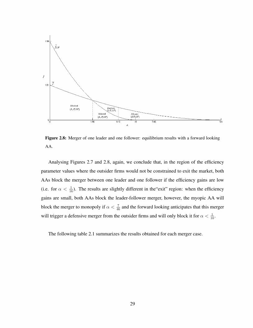
Figure 2.8: Merger of one leader and one follower: equilibrium results with a forward looking

AA.

Analysing Figures 2.7 and 2.8, again, we conclude that, in the region of the efficiency

parameter values where the outsider firms would not be constrained to exit the market, both

AAs block the merger between one leader and one follower if the efficiency gains are low

(i.e. for α < 116

). The results are slightly different in the“exit” region: when the efficiency

gains are small, both AAs block the leader-follower merger, however, the myopic AA will

block the merger to monopoly if α < 746

and the forward looking anticipates that this merger

will trigger a defensive merger from the outsider firms and will only block it for α < 110

.

The following table 2.1 summarizes the results obtained for each merger case.

29

Table 2.1: Efficiency gains results, by region and by AA for each merger case

Myopic AA Forward Looking AA

No Exit Exit No Exit Exit

Cournot0 < α < 1

14: No Proposal 1

14< α < 3

22: Block {2} 0 < α < 1

14: {1,1,1,1} 1

14< α < 1

5: Allow {2,2}

114

< α < 16

: Allow {2,1,1} α > 322

: Allow {2} 114

< α < 16

: Allow {2,2} α > 15

: Allow {1}

2L (CS)0 < α < 1

22: Block {2L,F,F} 1

22< α < 7

46: Block {2L} 0 < α < 1

22: Block {2L,F,F} 1

22< α < 5

74: Block {2L,2F}

122

< α < 110

: Allow {2L,F,F} α > 746

: Allow {2L} 122

< α < 110

: Allow {2L, F,F} α > 574

: Allow {2L,2F}

2L (SW)

0 < α < 0.00626: Block {2L,F,F} α > 122∧ f > f : Block {2L} 0 < α < 0.00626: Block {2L,F,F}

α > 122

: Allow {2L,2F}0.02334 < α < 1

10: Allow {2L,F,F} f > f : Allow {2L} 0.00626 < α < 5

194: Allow {2L, F,F}

5194

< α < 110

: Allow {2L, 2F}

2F0 < α < 1

10: Block {L,L,2F} 0.12848 < α < 7

46: Block {2F} 0 < α < 5

74: Block {L,L,2F}

α > 0.12848: Allow {2L,2F}110

< α < 16

: Allow {L,L,2F} α > 746

: Allow {2F} 574

< α < 16

: Allow {L,L,2F}

LF0 < α < 1

16: Block {L,F,LF} 1

16< α < 7

46: Block {LF} 0 < α < 1

16: Block {L,F,LF} 1

16< α < 1

10: Block {LF,LF}

116

< α < 18

: Allow {L,F,LF} α > 746

: Allow {LF} 116

< α < 18

: Allow {L,F,LF} α > 110

: Allow {LF,LF}

2.6 Conclusion

In this paper we investigate the role of efficiency defence argument in a setting where mergers

involve firms with asymmetric strategic power and the merger formation game encompasses

the AA as an active player.

We study and compare the decisions of two different types of AA: first, we assume a

myopic AA, which accepts or rejects a given merger without considering that this merger

may be followed by other mergers; and, second, a forward looking AA, which anticipates the

final industry structure a merger will give rise to if approved. By so doing, we conclude that

the decisions of these two types of AAs turn out to be very different, for all studied two-firm

merger cases, when the proposed merger would induce outsiders to exit the market, in the ab-

sence of a subsequent merger. When this is the case, the myopic AA would not authorise any

merger proposal when the associated efficiency gains are sufficiently low, since it assumes

that the resulting merged entity would monopolize the industry. The forward-looking AA,

however, correctly anticipates that the first (proposed) merger will be followed by a merger

involving the outsider remaining firms and, therefore, makes a decision anticipating the fi-

nal industry structure the first merger will lead to if approved. By so doing, the forward

30

looking AA decides to approve a merger involving two leaders or a leader and a follower

if the induced efficiency gains are high enough, and decides to approve a merger between

two followers even if the resulting efficiency gains turn out to be low. Notice that when two

leader firms or one leader and one follower firm merge, the resulting merged entity will be a

leader in the post-merger industry structure, implying that it can explore more its enhanced

efficiency by making use of its first-mover advantage. Even if for the three merger cases

the final market structure is the same (2L, 2F) the decisions of a forward looking AA when

deciding whether or not to accept the merger of two leaders knowing that this is going to

be followed by a merger of two followers are different than when the first merger is of two

followers and followed by a defensive merger of two leaders. Interestingly, the two types of

AAs are shown to instead adopt similar behaviour when a merger is not supposed to trigger

exit by outsider firms if approved (and no further merger takes place). When this is the case,

and for all possible two-firm merger proposals, the AA will, regardless of its type, require

that induced efficiency gains are sufficiently high, so as to approve the proposed merger. Ob-

viously, the forward looking AA anticipates whether a subsequent merger will occur or not,

but the decisions of the two types of AAs regarding the first merger proposal end up being

qualitatively very similar.

Comparing these results with those obtained with symmetric strategic power (see Motta

and Vasconcelos (2005)), we conclude that, when firms compete a la Cournot, the two-firm

merger is not going to be proposed to the myopic AA, for low levels of the efficiency gains.

A different outcome is obtained when firms compete instead a la Stackelberg. In this case,

firms propose the merger for all levels of the efficiency gains. Further, differently from what

happens under Cournot competition, we find that, even without efficiency gains, a two-firm

merger is always profitable under Stackelberg. Additionally, the forward-looking AA has

similar behaviour under Cournot and in the two-follower Stackelberg merger case. However,

we note that in the two leaders or one leader and one follower merger cases the AA is more

severe and restrictive in a Stackelberg industry than in a Cournot industry due to the fact that,

in some specific circumstances, it does not allow the defensive merger or it blocks the merger

for a larger range of the efficiency parameter.

31

Further, we find that the myopic AA decisions, when evaluating a two-leader merger,

are very similar when it considers the SW or the CS standards. Regardless of the adopted

standard, the myopic AA always blocks the merger involving the two leaders for low levels

of the efficiency gains. Moreover, the decisions of the forward looking AAs are quite different

for each adopted standard, when outsider follower firms are confined to exit the market. In

this case, although the SW-maximizer AA always accepts the merger, the CS-maximizer AA

blocks it for low levels of the efficiency gains. Also, we conclude that the CS-maximizer AA

(myopic or forward-looking) is more restrictive when evaluating merger proposals than the

SW-maximizer AA.

Finally, not only the merger’s cost savings but also the fact that firms have different strate-

gic power may affect AA decision on merger cases. The framework and the assumptions we

have assumed are of a particular kind. Further research on the analysis of AA intervention

should consider what happens if there is an asymmetric information problem between the AA

and the merging firms concerning efficiencies due to mergers. Also, it would be interesting to

assume more than two leaders or two followers in the market. This would change the results

of merger profitability and the intervention of an AA that assesses mergers according to a

consumer surplus standard. We think that these are very interesting and useful subjects for

further research.

32

Appendix

A.1. Social Welfare Approach

A.1.1. Merger of two leaders under a Myopic AA

Analysis of Stage 2 First the AA has to decide whether or not to allow the merger, if the

merger has been submitted for approval.

• If α < 110

and f < f2L, then outsider follower firms are able to make positive profits

after the merger has taken place. If this is the case, then the AA decides to authorise

the submitted merger if the total social welfare increases:

SW (2L, F, F ) ≥ SW (L,L, F, F ),

which is equivalent to

α > 18115

√31− 199

230≈ 0.00626.

Since we are in region where α < 110

, hence the AA will require that the efficiency

gains are sufficiently high in order to authorise the merger between to leaders, that is18115

√31− 199

230≈ 0.00626 ≤ α < 1

10.

• If, instead, α ≥ 110

or α < 110

and f2L < f < f , hence the merger induces outsiders

to exit the industry and therefore the industry is characterized by a single monopo-

list. Now the AA will decide to reject the merger of two leaders if the social welfare

decreases, that is:

SW (2L) < SW (L,L, F, F )⇔ f < 4148α2−1588α+771296

≡ f .

Hence, the AA rejects the merger if f2L < f < f and f < f .

33

Analysis of Stage 1 The analysis of Stage 1 is the same as before.

• If α < 110

and f < f2L, then outsider follower firms are able to make positive profits

after the merger has taken place. Hence, insider leader firms will always submit the

merger however this will be blocked by the myopic AA for low levels of the efficiency

gains.

• If, instead, α ≥ 110

or α < 110

and f2L ≤ f < f, hence the merger gives rise to very

high synergies that leads to the two outsider leader firms to want to exit the market.

Also after the merger, the outsider fringe firms will have negative profits. Hence, the

merger induces outsiders to exit the industry and therefore the industry is characterized

by a single monopolist. Therefore, the two leader firms will always submit the merger

to AA.

A.1.2. Merger of two leader firms under a forward looking AA

Analysis of Stage 4 The AA decides whether it wants to authorise the defensive merger

between outsiders (followers) of the first merger. Here we have two situations:

• If α > 110

or α < 110

and f2L < f < f , the followers will exit the market if the defensive

merger is rejected. The resultant market structure is {2L}. Hence, the defensive merger

is always approved if:

SW (2L, 2F ) > SW (2L)⇔ f < 3(1−2α)2

64≡ f .

However, f is always above f and f2L. Hence, the defensive merger is always approved

in this region.


and f < f2L, the followers will not exit the market if the defensive

merger is rejected. The AA will decide to block the merger between two followers if:

SW (2L, 2F ) ≤ SW (2L, F, F )⇔ α < 5194≈ 0.02577

34

Hence, this implies that the defensive merger will always be blocked if α < 5194

and

f < f2L.

Analysis of Stage 3 The analysis of Stage 3 is the same as before.

• If α ≥ 110

or α < 110

and f2L < f < f , the followers will leave the market if the

defensive merger is rejected. Hence, the defensive merger is always proposed if

πF (2L, 2F ) ≥ 0⇔(

1−2α4

)2 − 2f ≥ 0,

which is true for all α.

• If α < 110

the followers are not constrained to exit the market if the defensive merger is

rejected. Therefore, followers will merge if:

πF (2L, 2F ) =(

1−2α4

)2 − 2f ≥ 2πF (2L, F, F ) = 2[(

1−10α6

)2 − f]⇔

α ≤ 12191

√2 + 31

382= 0.17.

Thus, the defensive merger is always going to be proposed however the follower firms

anticipate that the defensive merger is blocked by the AA in the following stage when

α < 5194

.

Analysis of Stage 2 In this stage, the AA has to decide whether or not to allow the merger

of two leaders, if the merger has been submitted for approval.

• If α ≥ 110

or α < 110

and f2L < f < f , the AA anticipates that the merger between two

followers is approved. Hence, the AA will authorise the merger between two leaders

if:

SW (2L, 2F ) ≥ SW (L,L, F, F )⇔

0.01254 ' − 72781

√3 + 269

1562≤ α ≤ 72

781

√3 + 269

1562' 0.33189.

35

• If α < 110

and f < f2L, the followers will not leave the market, the AA anticipates that

the merger between two followers is blocked if α < 5194

. Hence, the AA will authorise

the merger between two leaders if:

α ≥ 18115

√31− 199

230≈ 0.00626

Analysis of Stage 1 Also, Stage 1 is the same as before. Leader firms will always submit

the merger in both regions.

36

Chapter 3

Mergers in Stackelberg Markets with

Efficiency Gains

This chapter is published in Journal of Industry Competition and Trade, September 20141

3.1 Introduction

Horizontal mergers are often seen as anticompetitive and harmful to social welfare because

they increase market concentration by eliminating at least one competitor in the market and

by creating entry barriers. However, a merger can also be welfare-enhancing if it generates

efficiency gains, increases incentives for innovation or creates synergies and scale economies

among firms.

In this paper, we analyze mergers’ profitability, the so called free-riding problem and the

merger induced effects on social and consumer welfare in a setting where: (i) firms are in

a Stackelberg market; and (ii) mergers can create cost heterogeneity between the remain-

ing firms in the industry. The literature on profitability and welfare effects of horizontal

mergers involving firms competing a la Stackelberg includes important contributions by:

Daughety (1990), Feltovich (2001), Huck et al. (2001), Heywood and McGinty (2007, 2008),

1This chapter benefited a lot from comments of anonymous reviewers from JICT and of the seminar partic-

ipants at the UECE Lisbon Meetings: Game Theory and Application in Lisbon, 2013.

37

Escrihuela-Villar and Faulı-Oller (2007) and Brito and Catalao–Lopes (2011).2 The main

message of these papers is that different types of mergers may occur in an industry charac-

terized by Stackelberg competition, that is, mergers may occur when firms have asymmetric

strategic power. In particular, one can observe mergers between leaders, mergers between

followers or even mergers between leaders and followers that give rise to a leader. It should

be highlighted, however, that these papers differ on the type of cost function assumed by the

authors. Daughety (1990), Feltovich (2001), Huck et al. (2001), Escrihuela-Villar and Faulı-

Oller (2007) considered a linear cost function while Heywood and McGinty (2007, 2008) and

Brito and Catalao–Lopes (2011) assumed a convex cost function.3 To the best of our knowl-

edge, however, none of these previous studies has addressed the role played by efficiency

gains when mergers involve firms in Stackelberg markets with linear costs.

In this paper, we contribute to cover the gap in this literature by showing that conclusions

about merger profitability, social welfare effects and the existence of a free-riding problem

crucially depend on whether the merger creates synergies, allowing firms to produce using a

more efficient technology after the merger takes place. In particular, we show that allowing

for merger induced synergies in Stackelberg markets (i) increases the incentive for mergers

by reducing the free rider problem associated with mergers (that outsiders benefit more than

insiders when a merger take place), and (ii) implies that profitable mergers can be welfare

improving also in a setting with linear costs. The intuition is that variable cost synergies

2Other strands in the literature also tried to solve the Salant et al. (1983)’s merger’s paradox and studied

the induced welfare effects and the free-riding problem of horizontal mergers by adopting Bertrand competition

with product differentiation (Deneckere and Davidson, 1985), Cournot competition with convex costs (Perry

and Porter, 1985), spatial competition (Rothschild et al., 2000) or by changing the properties of the demand

function (Faulı-Oller, 2002).3Heywood and McGinty (2008) showed that the combination of convex costs and leadership can largely

eliminate the merger paradox. Daughety (1990) showed that a merger between two followers is potentially

profitable and that this merger may be welfare-improving. Huck et al. (2001) and Feltovich (2001) concluded

that if a leader merges with a follower, the merger is unambiguously profitable. Further, Escrihuela-Villar and

Faulı-Oller (2007) assumed that followers are less efficient than leaders and showed that leaders rarely have

incentives to merge and that mergers among followers become profitable when the followers are inefficient

enough.

38

associated with mergers imply that the merged entity increases its output and that rivals then

expand less, which makes the merger more profitable. Moreover, the more aggressive be-

haviour by the merged entity implies that consumers will be less hurt by the merger.

Although this paper encompasses a theoretical exercise, it is also motivated by the prof-

itability of real-world mergers involving firms with asymmetric strategic power. A case in

point is the DRAM (Dynamic Random Access Memory) industry, where the leading man-

ufacturers announce their production plans in advance and manufacturers, which enter the

market later, respond by adjusting their quantity of DRAM produced. In addition, in this

specific industry, the last decades have witnessed a wave of mergers.4 Another example is

Microsoft’s dominance in software markets. In this case, although Microsoft usually makes

decisions first, other smaller companies typically react to Microsoft’s actions when making

their own decisions. Obviously, these subsequent followers’ actions, in turn, affect Microsoft

(see e.g. Graham (2013)). In both examples, it seems reasonable and plausible to analyze the

induced impacts of Stackelberg mergers.

The remainder of the paper is organized as follows. Section 3.2 introduces the baseline

assumptions of the model and presents the pre-merger results. Section 3.3 shows the effects

induced by the mergers. In Section 3.4 we present and discuss the results of the numerical

simulation. Finally, Section 3.5 concludes. All proofs are relegated to the Appendix.

3.2 Baseline Model

We consider an industry with n firms producing a homogeneous product, where m are leader

firms and n−m are follower firms. We assume a two-stage game. The sequence of firms’ de-

cisions is as follows. First, all leaders simultaneously choose their quantity, then all followers

simultaneously choose their quantity, after observing the leaders’ decision. Firms compete in

quantities over a linear demand P = 1−Q, where Q = Qm +Qn−m, Qm and Qn−m denote,

respectively, the total quantity produced by leader and follower firms and P is the industry

price.

4For details, see Escrihuela-Villar and Faulı-Oller (2007) and the references cited therein.

39

What distinguishes firms is not only their strategic power (being leader or follower) but

also the amount of capital they own. Hence, the cost function of firm i, which owns ki units

of the industry capital and produces qi units of output, is given by:5

C(qi, ki, α) =αK

kiqi (3.1)

where α ≥ 0 andn∑i=1

ki = K.

The total supply of capital is assumed to be fixed to the industry (and equal to K units,

where K = n). By assuming that the total quantity of capital available in the industry is

fixed, we are also assuming that, in this industry, entry is very difficult. Further, we are also

going to assume that there is no exit (see Assumption 3.2). We assume that each firm operates

with a constant marginal cost of production, but the level of its marginal cost is a decreasing

function of its capital holdings, ki.

Before the merger, although firms have asymmetric strategic roles they are cost symmet-

ric, holding one unit of capital each. After a two firms merger, however, firms still have

asymmetric strategic roles but are cost asymmetric: outsiders still own one unit of capital

each, whereas insiders are endowed with two units of capital.6 Hence, in this setting, the

merger brings the capital of merging parties into a single larger firm and, therefore, gives rise

to efficiency gains by decreasing the cost of the merging firms.7 The insider firm benefits

from some merger-specific cost savings, captured by the parameter α. The higher the value

of α is, the stronger the efficiency gains induced by a merger are and, therefore, the higher

is the cost reduction after the merger. Although merged firm’s level of capital is exogenous

and equal to the number of insider firms (ki = 2), the level of efficiency gains obtained will

5This is a simplified version of the cost structure proposed by Motta and Vasconcelos (2005) and captures

the specific case studied in Horn and Persson (2001a,b).6Differently from this paper, Catalao–Lopes (2007, 2008) studied mergers’ effects when firms have sym-

metric strategic roles but are pre-merger cost asymmetric. Similar to this paper, however, Catalao–Lopes (2007,

2008) assumes that, after the merger, the merged firm becomes more efficient than outsiders.7This feature of a merger was proposed by Perry and Porter (1985). In their framework firms’ marginal cost

is linear in output and mergers reduce the variable costs of production. For a discussion on the literature that

models mergers as the pooling of capacities see, for instance, Brito and Catalao–Lopes (2006).

40

depend on the type of the merger. Also, note that the marginal cost (C ′) variation is given by

∆C ′(qi, ki, α) = −αKki

= −αK2

. Since K is fixed and ki = 2, then |∂∆C′(qi,ki,α)∂α

| > 0, i.e.,

the higher is the level of cost savings, the lower is the cost after the merger, and therefore the

greater is the absolute change in the marginal cost.

Additionally, we assume that the fixed costs are zero, such that the elimination of a firm

does not create a further incentive to merge.8 Therefore, by setting the fixed costs to zero,

we are isolating the impact of cost savings on firms’ incentives to merge, on the free-riding

incentives and on both consumer and social welfare.

3.2.1 Pre-merger equilibrium

We consider that, before the merger, there are m < n Stackelberg leaders who independently

and simultaneously decide their individual quantity. The remaining n−m firms are Stackel-

berg followers who decide upon their quantity after learning about the total quantity supplied

by the leaders. Before the merger (BM), the equilibrium profits for leader and follower firms

are, respectively, given by:9

πBMLi (n,m, α) =(1− nα)2

(m+ 1)2 (n−m+ 1), for i = 1, ..,m. (3.2)

πBMFj (n,m, α) =(1− nα)2

(m+ 1)2 (n−m+ 1)2 , for j = 1, .., n−m. (3.3)

Additionally, the consumer surplus, the producer surplus and the social welfare are given

by:

CSBM =1

2

[n+m(n−m)]2 (1− nα)2

(m+ 1)2 (n−m+ 1)2 (3.4)

8Usually, in constant marginal cost models it is assumed that all firms in the market have identical costs and

that there are no fixed costs. Differently, in a Cournot setting, Catalao–Lopes (2008) studies the formation and

stability of mergers where firms are asymmetric and face fixed production costs. After a two firms merger, only

one fixed cost subsists. Catalao–Lopes (2008) shows that the existence of fixed costs increases the desirability

of merging and may also increase its stability. Perry and Porter (1985), on the other hand, showed that assuming

a positive fixed cost does not change the incentives to merge, since the insider firm would keep the fixed costs

of each of its pre-merger constituent firms.9For α = 0, these results are the same as those obtained by Huck et al. (2001) and Feltovich (2001).

41

PSBM =[n+m(n−m)] (1− nα)2

(m+ 1)2 (n−m+ 1)2 (3.5)

SWBM =1

2

[n+m(n−m)] [n+m(n−m) + 2] (1− nα)2

(m+ 1)2(n−m+ 1)2(3.6)

Assumption 3.1. Let us assume that

α <1

n≡ α (3.7)

This condition is imposed in order to exclude the case in which firms will not produce at

the status quo industry structure.

3.3 Merger Effects

In this section we analyze the effects of a merger between two firms in the industry on the

profits of both outsider and insider firms, and on both social welfare and consumer surplus.

If the merger occurs, then a larger and more efficient firm is created, owning ki = 2 units of

the industry capital.

The effects of a merger in the Stackelberg industry will depend on the types of the merger

partners involved. We consider three cases: a) merger of two leaders that form a more efficient

leader, b) merger of two followers, where the resulting firm behaves as follower and c) merger

of one leader and one follower, where the new firm behaves as leader after the merger takes

place. We do not analyze the case where two followers merge and the resultant firm is a

leader. When a leader merges with a follower in a market where firms compete in quantities,

it is reasonable to expect that the merged entity will behave as a leader, mainly for two

reasons: (1) the merged firm can still use the old commitment technology of the former

leader firm; and (2) it can be checked that the merged firm would always rather be a leader

than a follower. However, when two followers merge it is not so straightforward to explain

why two followers should gain this commitment power by merging. Although the resultant

firm becomes more efficient than its rivals, this does not mean that the merger allows firms

to change their strategic power. Daughety (1990) studies mergers between two followers

42

that give rise to a leader using linear costs, but he does not address why the merger changes

the behaviour of the firms neither considers the possibility that the merger could generate

efficiency gains. With convex costs, this case is analyzed by Brito and Catalao–Lopes (2011).

This means that in case a) the post-merger market will have m− 1 leaders but still n−m

followers, in case b) the post-merger market will havem leaders but only n−m−1 followers,

and in case c) the post-merger market will have m leaders and n−m− 1 followers.10

Assumption 3.2 is introduced to ensure that after any merger, the remaining firms in

the industry are all active. The motivation behind this assumption is that, in practice, exit

inducing mergers are very rare. Relaxing this assumption would significantly complicate

the analysis, since we would have to consider not only growth by mergers but also growth

by capital accumulation. In this case, we would obtain two regions of analysis: one region

where the merger would trigger the exit of outsider firms and the other region where the

reverse would occur. In addition, although mergers decrease competition, we exclude the

case where the merger leads to industry monopolization.

Assumption 3.2. Assume that after any two firms merger, all firms are active. That is, for all

α > 0 and knowing that α1 (n,m) < α3 (n,m) < α2 (n,m):

• Let α < α1 (n,m) ≡ 2n(n−m+3)

, such that all firms produce a positive amount after a

merger involving two leaders;11

• Let α < α2 (n,m) ≡ 23n

, such that all firms produce a positive amount after a merger

involving two followers and

• Let α < α3 (n,m) ≡ 2n(n−m+2)

, such that all firms produce a positive amount after a

merger involving one leader and one follower.

10See Appendix B.1 for further information on post-merger equilibrium results.11Note that in order for the insider’s quantity to be positive, the level of efficiency gains should be higher than

a negative threshold. Since we have assumed that α > 0, we exclude this threshold. Also, it is straightforward

to show that the quantity of insider firms is always positive for any level of efficiency gains. However, in order

for both outsider leader or follower firms to produce, α must be lower than α1. See Remark 3.1, Appendix B.1.

43

For instance, if the level of efficiency gains exceeds α1 (n,m), then, in a symmetric equi-

librium, both outsider follower and leader firms would exit the market after the merger be-

tween two leaders. Consequently, the monopoly would be the merger induced industry struc-

ture. In addition, if exit inducing mergers were possible, the total industry capital could

change after a merger. This being the case, the model would probably need to be extended so

as to allow for firms to buy and sell capital. This is, however, outside the scope of the present

paper since we want to focus on growth by acquisition only.

The following subsections discuss the impact of each merger on the profitability of insid-

ers and outsiders and on consumer surplus and social welfare. Further, we compare some of

the results obtained with those obtained if firms were competing a la Cournot or if there were

no efficiency gains generated by the mergers.

3.3.1 Insiders’ Profitability

In this subsection we show that mergers in industries where firms have asymmetric strategic

power may actually be profitable.

In order to assess mergers’ profitability it is necessary to compare, for each merger case,

the profits obtained when firms operate independently with the equilibrium profits of the

merged entity.

Let the change in insider profits due to the merger be expressed as g(n,m, α), where g

is different for the different merger cases. For a specified number of leader firms (m) and

follower firms (n−m), this expression can be used to determined whether the merger of two

firms is profitable. Now, for each merger case, gains from the merger occur if and only if

g(n,m, α) > 0.

The merger between two leaders is profitable if the profit of the insider leader firm (π2LLI

)

is higher than the aggregate profit of the leader firms before the merger, that is, if and only if:

g2L(n,m, α) = π2LLI

(n,m, α)− 2πBMLi (n,m, α) > 0

g2L (n,m,α) =[2− nα(n−m(n−m+ 2) + 3)]2 (m+ 1)2 − 8m2 (1− nα)2

4m2 (n−m+ 1) (m+ 1)2 > 0 (3.8)

44

The merger between two followers is profitable if the profit of the insider follower firm

(π2FFI

) is higher than the aggregate profit of the follower firms before the merger, i.e., iff:

g2F (n,m, α) = π2FFI

(n,m, α)− 2πBMFj (n,m, α) > 0

g2F (n,m,α) =[2− nα (3− (m+ 1) (n−m))]2 (n−m+ 1)2 − 8 (n−m)2 (1− nα)2

4 (n−m+ 1)2 (m+ 1)2 (n−m)2 > 0

(3.9)

The merger between a leader and a follower is profitable if the profit of the insider firm

(πLFI ) is higher than the aggregate profit of the outsider firms before the merger, that is, iff:

gLF (n,m, α) = πLFI (n,m, α)−[πBMFj (n,m, α) + πBMLi (n,m, α)

]> 0

gLF (n,m,α) =[2− nα (m (n−m)− 2)]2 (n−m+ 1)2 − 4 (n−m+ 2) (n−m) (1− nα)2

4 (n−m+ 1)2 (m+ 1)2 (n−m)> 0

(3.10)

Hence, the incentives for two firms to merge depend not only on the number of each type

of firms in the market but also on the efficiency parameter α.12 Propositions 3.1, 3.2 and 3.3

summarize, for each merger case, the profitability results.

Proposition 3.1. For allm > 1 and 0 < α < α1 (n,m), knowing that α4 (n,m) < α1 (n,m)

the merger between two leaders is profitable iff:

i) α > 0, for m = 2 and

ii) α > α4 (n,m) , for all m > 2.

Proof. See Appendix B.2. �

12By solving g2L (n,m,α) = 0, g2F (n,m,α) = 0 and gLF (n,m,α) = 0, we obtain the roots of α as a

function of n and m, that ensure merger profitability. However, some of these roots are negative or higher than

α and, therefore, we exclude them.

45

Proposition 3.2. For all n − m > 1 and 0 < α < α2 (n,m), knowing that α5 (n,m) <

α2 (n,m) the merger between two followers is profitable iff:

i) α > 0, for n−m = 2 and

ii) α > α5 (n,m), for all n−m > 2.


Proposition 3.3. For all n−m > 1 and m > 1 and 0 < α < α3 (n,m), the merger between

a follower and a leader is always profitable.


Not surprisingly, Propositions 3.1 and 3.2 confirm that a merger is profitable when it

involves the only two leaders or the only two followers in the industry. These mergers were

already profitable in the no synergies case and, therefore, their profitability is reinforced

when efficiency gains are induced by a merger and even when these efficiency gains are low.

However, these propositions also show that if there are more than two leader firms or more

than two follower firms in the status quo industry structure, mergers involving two leaders

or two followers can be profitable if the induced efficiency gains are high enough.13 Finally,

Proposition 3.3 states that there is always profit incentive for a leader and a follower to merge

if there are efficiency gains.

The results obtained in Propositions 3.1, 3.2 and 3.3 differ from those obtained without

merger-created efficiencies.14 When mergers do not create any synergies, the results obtained

in our framework are the same as those previously shown by Huck et al. (2001) and Feltovich

(2001). In particular, a merger of two leaders to form a leader or two followers to form a

follower is profitable if and only if the merging firms were the only firms of their type at

the status quo industry structure (Huck et al. (2001)’s Proposition 1 and Feltovich (2001)’s

13This result is similar to the one obtained by Perry and Porter (1985), where firms compete a la Cournot

and costs are convex. This is also similar to Heywood and McGinty (2007)’s paper, where they conclude,

under convex costs, that mergers involving two leaders or two followers are profitable if the costs savings are

sufficiently high.14See Appendix B.3 for further information.

46

Result 1). However, if one leader and one follower merge to form a leader, the merger is

always profitable since now the follower firm benefits from an increase in its strategic power

(Huck et al. (2001)’s Proposition 2 and Feltovich (2001)’s Result 3). Moreover, if there is

no strategic power advantage for any firm (Cournot competition), we obtain the well known

Salant et al. (1983)’s result: a merger between two firms with the same strategic power that

creates a firm of the same type is always unprofitable for the merging firms, unless more

than 80% of the firms in the industry merge or there are sufficiently high fixed costs. The

difference between our results and its analogy to the Cournot model is that, in our setting, in

order for a merger to be profitable, the merging firms do not need to be the only two firms

in the industry nor the only firms of their type in the industry. Further, it can be shown that

when there are no efficiency gains, the incentives for two firms to merge are higher when firms

compete a la Stackelberg than in the case of Cournot competition. Hence, the asymmetric

strategic power combined with merger efficiency gains creates a larger incentive for firms to

merge.

Figure 3.1 illustrates the results regarding merger profitability, for each merger case, when

n = 6 and m = 3.

Figure 3.1: Merger profitability for n = 6 and m = 3

47

Two remarks should be made regarding this figure. First, merger profitability is positively

correlated with the level of efficiency gains induced by the merger, as expected.15 Second,

for a given level of efficiency gains, the merger’s impact on insiders’ profitability is more

significant when (at least one of these) insiders have a leadership position in the market.

The same results are obtained if we considered any other feasible values for n > 2 and m.

Further, when there are efficiency gains, the effect of these efficiency gains on merger prof-

itability is higher when the merger is between two leader firms (or a leader and a follower

firms) than when the merger is between two follower firms, that is, ∂g2L(n,m,α)∂α

> ∂g2F (n,m,α)∂α

and ∂gLF (n,m,α)∂α

> ∂g2F (n,m,α)∂α

. The reason why the profitability of a merger involving at

least one leader is more positively affected by merger induced synergies than the profitability

of a merger involving two followers is simple. When the merged entity will be a leader in

the post-merger industry structure, its higher efficiency will be crucial to explore further the

Stackelberg (first-mover) advantage. If instead we investigate the impact of merger efficien-

cies on the profitability of two alternative mergers where a leader firm is always involved,

then the conclusion is no-longer clear-cut. If α is low, the effect of the efficiency gains on

merger profitability is higher when the merger is between a leader and a follower firm than

when the merger is between two leader firms, i.e., ∂g2L(n,m,α)∂α

< ∂gLF (n,m,α)∂α

. However, the

reverse occurs as α increases.

Additionally, the sequentiality of the choices plays an important role in explaining merger

profitability. In a merger involving two followers, the insider followers anticipate that outsider

(leader and follower) firms will reduce their quantities in response to the merger. This, in

turn, implies that the increase in the merged follower firm quantity will not be so great than

in the case where two leaders (or a leader and a follower) merge, even if cost savings result

from the merger, since now the insider firm has a follower position. If the merger involves,

instead, two leader firms, both insider leader and outsider leader firms make their output

decisions anticipating the subsequent followers’ best response. Thus, as mentioned above,

insider firms will be able to enhance merger profitability by combining synergies with their

15Note that for all merger cases the ∂g(n,m,α)∂α > 0 and that ∂

2g(n,m,α)∂α2 > 0. See Appendix B.2.

48

leadership position.

3.3.1.1 Numerical simulation results on merger profitability

By making use of numerical simulations, it can be illustrated that for m > 2 and n−m > 2,

keeping the level of efficiency gains and the number of followers constant, as the number of

leaders increases, the merger profitability increases in the three cases. Further, keeping the

number of leaders constant, as the number of followers increases, the merger profitability

decreases in the cases of a merger between two leaders and in a merger involving a leader

and a follower, i.e., ∂g2L(n,m,α)∂m

> 0, ∂g2L(n,m,α)∂n−m < 0; ∂g2F (n,m,α)

∂m> 0, ∂g2F (n,m,α)

∂n−m > 0;∂gLF (n,m,α)

∂m> 0, ∂g

LF (n,m,α)∂n−m < 0.

Plugging in specific values of n andm into the g2L (n,m, α), g2F (n,m, α) and gLF (n,m, α)

functions, allows solving for the critical value of α. The results of our simulations are pre-

sented in Table 3.1. Table entries are values of α that satisfy Propositions 3.1, 3.2 and 3.3

(lower bound) and Assumption 3.2 (upper bound), i.e. they identify the interval for the pa-

rameter α, such that the merger is profitable and exit is not induced by the merger. The top

entry is for a merger between two leaders, the middle entry is for a merger between two

followers, and the bottom entry is for a merger between a leader and a follower.

Table 3.1: Efficiency gains conditions for profitable mergers and no exit

Two remarks are in order at this point. First, keeping the number of leaders (followers)

49

constant, as the number of followers (leaders) increases, the range of the critical region of

the level of efficiency gains for two leaders (two followers) to profitably merge decreases.

Second, keeping the number of leaders (followers) constant, the range of the critical region

of the parameter α for a leader-follower to be profitable decreases as the number of follower

(leader) firms increases.

Hence, any two firms merger is more likely to be profitable when there are relatively

few firms of the same type of the merging firms but also few firms of the other type. In the

two-leader merger case, the merged leader firm wants to have few leader competitors and

to enjoy leadership over few follower firms. In the two-follower merger case, the merged

follower firm wishes to have few follower competitors (increasing the output in response to

their reduction) and to follow few leader firms. Also, as the number of firms of same type

(for instance, leaders) falls due to the merger (two-leader firms merger), there is a decrease

in the region of parameters α for which the merger is profitable.

Another result is that the range of the critical region of the parameter α required for two

leaders to profitably merge without exit does not exceed that necessary for the two followers

to profitably merge and also does not exceed that necessary for the merger between one leader

and one follower to be profitable. This means that, when there are efficiency gains the merger

between two leader firms is less likely to be profitable and satisfy Assumption 3.2 than the

mergers between two follower firms or between a leader and a follower firms.

Surprisingly, however, the range of the critical region of the parameter α required for

two followers to profitably merge exceeds that necessary for one leader and one follower to

profitably merge. Hence, when a merging firm behaves as a follower at the status quo industry

structure, it is more likely that it will benefit from a merger (generating efficiency gains) when

it merges with a firm of the same type than when it embarks on a merger with a firm of a

different type and enjoys leadership in the merger induced industry structure. This result may

be due to the fact that in the merger between a leader and a follower, the leader has already

a high profit at the status quo industry structure. Hence, the merger induced efficiency gains

will have to be substantial so as to convince this leader firm to accept to share its leadership

position with its merger partner (a follower) in the market structure induced by the merger.

50

Further, having two stages of quantity choice does not mitigate the reaction to the quantity

reduction undertaken by the merged firm but instead increases it, reducing the opportunities

for a two-leader merger, that generates efficiency gains, to be profitable under Stackelberg

than a two firms merger under Cournot.16 However, for the two-follower merger the reverse

occurs. Hence, we conclude that, when each merger is profitable, the profitability under

Stackelberg could be higher or lower than under Cournot, for different merger cases and

levels of efficiency gains.

Hence, the asymmetric strategic power combined with merger induced efficiency gains

can indeed increase firms’ incentives to merge.

3.3.2 Free-riding problem

In this subsection we analyze whether outsider firms profit more from the merger than the

insider firms. If this is the case, although insiders’ profits increase with the merger, firms

would prefer to wait for their rivals to merge and, thus, benefit from higher prices without

having to reduce the quantity. To verify if there is a free-riding problem in our setting, we

compare, for each merger case, the profits of the insider firm with the profits of the outsider

firms that could also participate in the merger, conditioning on each merger being profitable

and excluding the case where outsider firms do not produce.

To identify the free-riding problem, define f(n,m, α) as the difference between the profits

of the outsider firms and the profit of the insider firm, that depends on the number of leader

(m) and follower (n −m) firms and on the level of cost savings (α). For each merger case,

outsider firms profit more from the merger than the insider firms if and only if f(n,m, α) > 0.

When the merger between two leaders (followers) creates no synergies, outsider leader

(follower) firms have always incentives to free-ride and, thus, always would prefer to wait

for their rivals to merge, benefiting from higher prices without having to reduce the quan-

tity. Also, when the merger is between a leader and a follower, outsider firms have always

incentives to free-ride on it. These results are similar to those obtained under Cournot. In16More details on calculations for a Cournot market can be provided upon request to the authors.

51

both settings, and without cost savings, the outsider firms benefit more from the merger than

the insider firms, and these benefits may be higher under Cournot than under Stackelberg,

depending on the number of firms in the market.

For each merger case, let αA3.2 be the level of efficiency gains obtained in Assumption 3.2.

Proposition 3.4 summarizes under which conditions it is better to free ride than to participate

in the merger.

Proposition 3.4. For all n > m and 0 < α < αA3.2, knowing that α8 < α6 < α7, when

mergers create synergies:

i) The merger between two leaders gives rise to a free-riding problem if outsider leader

firms earn more than the insider (f 2L(n,m, α) > 0), that is, iff:

α < α6(n,m), for all m ≥ 2;

ii) The merger between two followers gives rise to a free-riding problem if outsider fol-

lower firms earn more than the insider (f 2F (n,m, α) > 0), that is, iff:

α < α7(n,m), for all n−m ≥ 2;

iii) The merger of one follower and one leader gives rise to a free-riding problem if outsider

firms earn more than the insider (fLF (n,m, α) > 0), that is, iff:

α < α8(n,m), for all n−m > 1 and m > 1;

where α6(n,m), α7(n,m) and α8(n,m) are lower than αA3.2.


Hence, it turns out that when there are cost savings created by the merger, for some merger

cases the free-riding problem is solved whereas for others it is not. While the profit of the

merged firm always increases, that of an outsider firm may either increase or decrease as a

result of the merger.

In traditional models, without merger cost’s savings the profit of the outsider firms in-

creases after the merger. The merged firm increases its profits by decreasing the quantity,

which, in turn, also increases outsiders’ profits. However, with linear costs and cost syner-

gies the insider firm may actually increase quantity beyond that of its pre-merger constituent

52

firms and, therefore, the quantity and profits of outsider firms may decrease after the merger.

For instance, if the merger is between two followers, the insider firm will produce more and

both outsider follower and leader firms will react by reducing their quantity. This reduction

is higher as the level of efficiency gains increases. Hence, for high level of efficiency gains,

outsider firms have no incentives to free ride on the merger.

Hence, we find that when the merger creates cost synergies and firms in the industry have

asymmetric strategic power, the free-riding problem might disappear. This result is similar

to the one obtained by Heywood and McGinty (2008), with convex costs and Stackelberg

leadership. However, this contrasts with Perry and Porter (1985), Huck et al. (2001), Hey-

wood and McGinty (2007) and Brito and Catalao–Lopes (2011). In these papers, outsider

firms would always prefer to remain as outsiders, even when the merger is profitable for the

insiders.17

In sum, we find that when there is a merger between two leaders, two followers or a

leader and a follower, outsider firms have no incentives to free-ride if the merger generates

sufficiently cost savings.

3.3.3 Consumer Surplus and Social Welfare

In the next subsections we examine the effects of each merger case on both social welfare

and consumer surplus.

17For instance, the model of Brito and Catalao–Lopes (2011) is significantly different from ours. In particu-

lar, they study the effects of the merger between two followers that become a leader. In addition, they consider a

convex cost function and that after the merger firms have asymmetric costs. They show that under convex costs

there is a free riding problem. The merger between two followers that become leader decreases the number

followers. Now, this decrease of the number of followers has a negative effect on the profit of the merging

followers because one of them is eliminated, however it has a positive effect for outsider followers. Also, by

turning a follower into a leader induces a negative effect for outsider followers since increasing the number of

leaders by one always reduces each follower’s profit. Hence, Brito and Catalao–Lopes (2011) show that if the

cost effect is such that the negative effect on outsiders’ profits due to the appearance of more leaders is higher

than the positive effect due to the elimination of one follower, the free-riding problem emerges.

53

Williamson (1968) argued that the goal of competition policy should be to maximize

total welfare. Later, Farrell and Shapiro (1990) considered that mergers should be assessed

on the basis of their effects on consumers and firms jointly, assuming that the merger will be

privately profitable to the merging firms. However, as Lyons (2002) argued, “most antitrust

authorities operate under legislation and guidelines that reject the social welfare standard,

and no major antitrust authority seems to apply it consistently. Instead, antitrust authorities

tend to use the consumer surplus standard when evaluating merger cases”.

3.3.3.1 Consumer Surplus Standard

In this subsection we analyze the effects of each merger case on consumer surplus. We also

show how the consumer surplus variation depends on with the efficiency parameter α.

The consumer surplus variation is found by solving ∆CS = CSAM(n,m, α)−CSBM(n,m, α),

where the formal expressions regarding consumer surplus after and before the merger (CSAM

and CSBM , respectively) are presented in the Appendix.

When mergers create efficiency gains, the effects on consumer surplus are manifold, as

summarized in the following proposition.

Proposition 3.5. For all n > m and 0 < α < αA3.2, when mergers create efficiency gains:

i) The merger between two leaders improves consumer surplus iff:

α > α9 (n,m), for all m ≥ 2 and n−m > 1.

ii) The merger between two followers improves consumer surplus iff:

α > α10 (n, n), for all n−m ≥ 2 and all m > 1.

iii) The merger between a leader and a follower improves consumer surplus iff:

α > α11 (n,m), for m > 1 and n−m > 1.



Analyzing Proposition 3.5 we conclude that the merger between two leaders, two fol-

lowers or one leader and one follower can actually improve consumer surplus if the level of

efficiency gains is high enough.

54

The merged entity resulting from the merger of two leaders has a lower cost than outsiders

and this may actually increase the quantity beyond the quantity of its pre-merger constituent

firms. Also, outsider firms will react by reducing their quantity. However, the increase in

insider’s quantity may more than compensate for the decrease in outsiders’ quantity. Hence,

the net effect may then be a price decrease if the cost savings are sufficiently high. If the level

of efficiency gains are low, the reverse occurs. Hence, if the merger induced cost savings

are sufficiently high and satisfy the thresholds above, the merger could generate gains for

consumers by decreasing price and increasing total quantity in the market. This result is

similar to the one obtained by Farrell and Shapiro (1990) who have shown that, in a Cournot

framework, mergers are likely to harm consumers unless cost savings are sufficiently strong.

Interestingly, however, without synergies, all discussed types of mergers have the same

effect: the consumer surplus decreases. This is a similar result to the one obtained by Salant

et al. (1983) under Cournot competition. Without cost savings, any two firms merger always

leads to a decrease in the total quantity and, thus, increases the market price.

In Figure 3.2 we illustrate, for the case in which n = 6 and m = 3, the interval of cost

savings where each type of merger increases the consumer surplus.

Figure 3.2: ∆Consumer Surplus

55

As we can observe from Figure 3.2, the variation in the consumer surplus is positive for

all merger cases if the level of efficiency gains is high enough. Moreover, this relation is a

non-monotonic one.

In any case, in the relevant region of parameter values defined by Assumption 3.2, after

any two firms merger and for sufficiently high efficiency gains, the merged entity, due to its

increased efficiency, produces more and outsider firms react by decreasing their output. The

net effect then is an increase in the industry output and a decrease in the market price, leading

to an increase in consumer surplus.18

This figure also shows that the merger’s cost savings generate higher gains for consumers

when the resultant insider firm is a leader than when it is a follower. As already mentioned,

when the firm resulting from the merger is not only more efficient, but also enjoys a lead-

ership position, the total industry output will increase more than in a merger wherein the

resulting firm becomes more efficient but behaves as a follower in the merger induced in-

dustry structure. Additionally, when there are merger induced efficiency gains, there is a

greater likelihood that a merger between two leader firms (or a merger between a leader and

a follower firms) improves consumer surplus when comparing to the merger between two

followers, since the α9 (or α11) in Proposition 3.5 is always lower than α10.

Let us start by comparing the two mergers which do not affect the strategic power of

the firms involved. A merger between two leader (follower) firms, reduces the number of

leaders (followers) in the market. However, the insider leader (follower) firm becomes more

efficient than its rivals (leaders and followers). Since the strategic power of the insider does

not change, here the cost efficiency effect turns out to be stronger than the concentration

effect and the merger increases consumer surplus. Now, comparing the two merger cases, the

key difference is that the resulting firm has different strategic power in both cases. In the two

follower merger case, the insider firm is a follower and, therefore, this explains why the cost

savings affect less the increase in consumer surplus.

Consider now a merger involving a leader and a follower firm. When this is the case,

there are two effects at play induced by the merger: an increase in concentration (there is

18Note that, initially, ∂∆CS∂α > 0 when α < αA3.2. Also,∂

2∆CS∂α2 is always negative. See Appendix B.5.

56

a decrease in the number of follower firms) that tends to hurt consumer surplus, on the one

hand, and an increase in the efficiency of a merged entity that enjoys a leadership position

which benefits consumer surplus, on the other. As a result, there will be a reduction in the

quantity produced by all outsider firms (both followers and leader ones) whereas the merged

entity will expand output. The net effect is then an increase in the industry quantity (and a

corresponding decrease in market price). It should be noted, however, that the induced cost

synergies in this merger do no exceed those regarding a merger between two leaders.

3.3.3.2 Social Welfare Standard

In this subsection we examine the induced welfare effects of each merger and also show how

the welfare variation depends on the level of efficiency gains (as measured by α).

The welfare variation is found by solving ∆SW = SWAM(n,m, α)− SWBM(n,m, α).

The solution to this equation, for each merger, is a second order polynomial expression and

untractable. However, as we can see from the simulations (in Section 3.4), the results show a

consistent pattern.

When mergers create efficiency gains, the effects on social welfare are manifold. Proposi-

tion 3.6 summarizes the results obtained for social welfare when the mergers create efficiency

gains.

Proposition 3.6. For all n > m and 0 < α < αA3.2, when mergers create efficiency gains:

i) The merger between two leaders is welfare-enhancing iff:

α > α12 (n,m), for all m > 1 and n−m > 1;

ii) The merger between two followers is welfare-enhancing iff:

α > α13 (n,m), for n−m ≥ 2;

iii) The merger of one leader and one follower is welfare-enhancing iff:

α > α14 (n,m), for m > 1 and n−m > 1;



57

Proposition 3.6 states that a merger between two leaders, two followers or one leader and

one follower can actually improve the social welfare, for certain conditions on the efficiency

parameter.19 When the merger generates sufficiently high cost synergies, the insider firm will

produce more and hence the price decreases which, in turn, increases the consumer surplus.

On the other hand, the cost savings also give rise to an increase in merger profitability, which,

in turn, lead to an increase in the producer surplus of the insiders and a decrease in the

producer surplus of the outsiders. Hence, overall, and for certain levels of efficiency gains

there is an increase in the social welfare.

In concluding, it should be highlighted that, in a no-synergies scenario, as far as welfare

is concerned, all discussed types of mergers have the same effect: the social welfare de-

creases. This is the same result as in Feltovich (2001)’s and Huck et al. (2001)’s papers. In a

model without efficiency gains and linear costs, both Feltovich (2001) and Huck et al. (2001)

concluded that a merger between two similar firms that produces a firm of the same type is

welfare lowering since, despite the price and total profits increase, the quantity and consumer

surplus decrease. Additionally, Huck et al. (2001) show that when one big fish eats one small

fish (i.e., when a leader firm merges with a follower one), the price increases and the total

output decreases and so the net effect is also a decrease in social welfare. In addition, if firms

have the same strategic power, we obtain the Salant et al. (1983)’s Cournot results, which, in

this case, is the same as obtained when firms have asymmetric strategic power.20

3.4 Simulation Results

In this section we present and discuss the simulation results obtained for the different merger

cases, illustrating the results obtained in the propositions above. For simplicity, we assume

that there are n = 12 firms in the market, such that the critical parameters of α obtained in

19This is a similar result to the one obtained by Salant et al. (1983), under Cournot: when firms have the

same strategic power, a merger that generates cost savings may also increase social welfare.20In a Cournot setting with asymmetric firms and fixed costs, Catalao–Lopes (2007) shows that mergers

may be socially desirable as long as the level of asymmetry is high enough. Also, if firms are not sufficiently

asymmetric, there is a decrease in social welfare, unless the fixed cost savings are high enough.

58

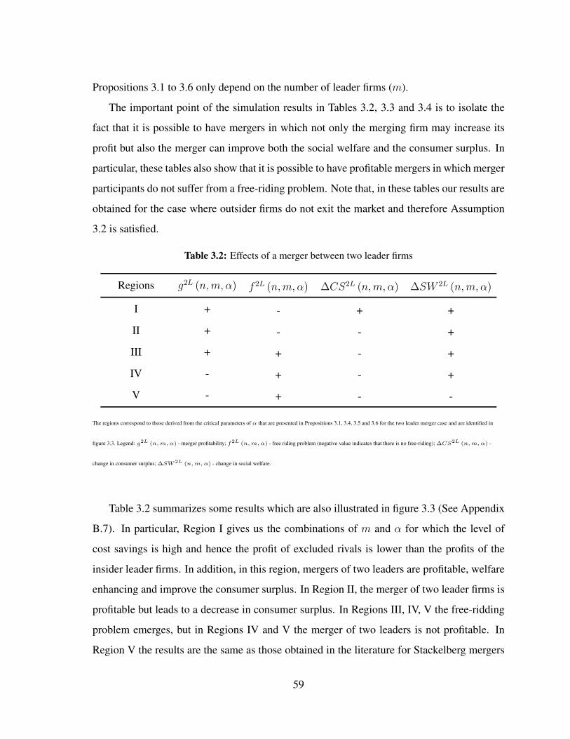
Propositions 3.1 to 3.6 only depend on the number of leader firms (m).

The important point of the simulation results in Tables 3.2, 3.3 and 3.4 is to isolate the

fact that it is possible to have mergers in which not only the merging firm may increase its

profit but also the merger can improve both the social welfare and the consumer surplus. In

particular, these tables also show that it is possible to have profitable mergers in which merger

participants do not suffer from a free-riding problem. Note that, in these tables our results are

obtained for the case where outsider firms do not exit the market and therefore Assumption

3.2 is satisfied.

Table 3.2: Effects of a merger between two leader firms

Regions g2L (n,m, α) f 2L (n,m, α) ∆CS2L (n,m, α) ∆SW 2L (n,m, α)

I + - + +

II + - - +

III + + - +

IV - + - +

V - + - -

The regions correspond to those derived from the critical parameters of α that are presented in Propositions 3.1, 3.4, 3.5 and 3.6 for the two leader merger case and are identified in

figure 3.3. Legend: g2L (n,m, α) - merger profitability; f2L (n,m, α) - free riding problem (negative value indicates that there is no free-riding); ∆CS2L (n,m, α) -

change in consumer surplus; ∆SW2L (n,m, α) - change in social welfare.

Table 3.2 summarizes some results which are also illustrated in figure 3.3 (See Appendix

B.7). In particular, Region I gives us the combinations of m and α for which the level of

cost savings is high and hence the profit of excluded rivals is lower than the profits of the

insider leader firms. In addition, in this region, mergers of two leaders are profitable, welfare

enhancing and improve the consumer surplus. In Region II, the merger of two leader firms is

profitable but leads to a decrease in consumer surplus. In Regions III, IV, V the free-ridding

problem emerges, but in Regions IV and V the merger of two leaders is not profitable. In

Region V the results are the same as those obtained in the literature for Stackelberg mergers

59

with symmetric costs: since efficiency gains are very low, mergers between two leader firms

are not profitable, face a free-riding problem, and decrease both consumer and social welfare.

Table 3.3: Effects of a merger between two follower firms

Regions g2F (n,m, α) f 2F (n,m, α) ∆CS2F (n,m, α) ∆SW 2F (n,m, α)

I + - + +

II + - - +

III + + - +

IV - + - +

V - + - -

VI + + - -

The regions correspond to those derived from the critical parameters of α that are presented in Propositions 3.2, 3.4, 3.5 and 3.6 for the two follower merger cases and are identified in

figure 3.4. Legend: g2F (n,m, α) - merger profitability; f2F (n,m, α) - free riding problem (negative value indicates that there is no free-riding); ∆CS2F (n,m, α) -

change in consumer surplus ; ∆SW2F (n,m, α) - change in social welfare.

Table 3.3 sums up the main results illustrated in figure 3.4 (See Appendix B.7). Again,

Region I gives us the combinations of m and α for which the merger of two followers is

profitable, improves both the consumer and social welfare, and the profits of outsider firms are

lower than the profits of the merged firm. Regions II, III, IV, V, VI gives us the combinations

of m and α for which the merger always decrease the consumer surplus. In Regions III, IV,

V, VI the free-ridding problem emerges, but in Regions IV and V the merger of two followers

is not profitable. Moreover, in Regions V and VI, since the level of efficiency gains are low,

the merger decreases both consumer and social welfare.

60

Table 3.4: Effects of a merger between a leader and a follower firms

Regions gLF (n,m, α) fLF (n,m, α) ∆CSLF (n,m, α) ∆SWLF (n,m, α)

I + - + +

II + - - +

III + + - +

IV + + - -

The regions correspond to those derived from the critical parameters of α that are presented in Propositions 3.3 to 3.6 for the leader follower merger case and are identified in figure 3.5.

Legend: gLF (n,m, α) - merger profitability; fLF (n,m, α) - free riding problem (negative value indicates that there is no free-riding); ∆CSLF (n,m, α) - change in

consumer surplus ; ∆SWLF (n,m, α) - change in social welfare.

Table 3.4 summarizes the main results illustrated in figure 3.5 (see Appendix B.7). In

all regions, the merger between a leader and a follower is always profitable. Region I gives

us the combinations of m and α for which the merger of a leader and a follower is always

profitable, welfare enhancing and improves the consumer surplus. Region II, III, IV gives us

the combinations of m and α for which the merger always decreases consumer surplus. In

Regions III and IV, although the merger between a leader and a follower firm is profitable,

outsider firms have incentives to free ride on it.

In concluding this section, we contrast the main qualitative results obtained with this

simulation exercise with those regarding the no-synergies benchmark case. In a scenario in

which there are no cost savings, although a merger between a leader and a follower is always

profitable, mergers between two leaders or two followers are profitable only if the merger

involves the only two leaders or the only two followers at the status quo industry. Moreover,

the three types of mergers should be objected by antitrust authorities because they reduce

both consumer and social welfare.

Some important implications are obtained when there are efficiency gains resulting from

the merger. These gains obviously enhance the profitability of any of the studied mergers, by

allowing the merged entity to benefit from a cost advantage over its rivals. Some of the results

61

presented on Tables 3.2, 3.3 and 3.4 are similar for the three merger cases. In particular, when

the level of efficiency gains is low (Regions IV or V), the merger between two firms is not

profitable (with exception in the leader-follower merger case), harms social and consumer

welfare and faces a free-riding problem. Therefore, antitrust authorities should discourage

such mergers. Further, we can also conclude that, in our framework, whenever a merger is

not profitable, it also does not increase consumer surplus. In addition, whenever the studied

mergers face free-riding problems, they also hurt consumer surplus.

If, however, efficiency gains induced by the merger are high, then the social welfare

actually improves for the three merger cases. In particular, there are some cases in which the

high cost saving allows firms to produce more at lower price, which, in turn, increases social

welfare by increasing both consumer surplus and producer surplus.

Additionally, we conclude that when efficiency gains are sufficiently high, almost all the

mergers that overcome the free-riding problem are also profitable and enhance social welfare,

a result that differs from the ones obtained in the previous literature. This contrasts with the

models considering Stackelberg leadership with linear costs such as Huck et al. (2001), in

which they conclude that all mergers reduce social welfare.

Our results reinforce important policy implications already highlighted in the literature.

When evaluating horizontal mergers, antitrust authorities should carefully evaluate whether

(i) the proposed merger is expected to give rise to important synergies; and (ii) what is the

strategic power of the firms involved in the merger proposal. This is clearly a challenging

and difficult task, but, as the previous analysis illustrates, the final induced impacts of a given

merger crucially depend on the interplay between these two very important factors.

62

3.5 Conclusion

This paper extends the literature on the incentives for and welfare effects of mergers in

oligopolistic markets where some firms are (Stackelberg) leaders and some are (Stackelberg)

followers by allowing for merger synergies.

Within this theoretical framework, we find that mergers involving two leaders, two fol-

lowers or a leader and a follower may be profitable, even if costs are linear, in a setting where

the merger may give rise to efficiency gains.

In case there are no efficiency gains from a given merger, then we show that the profitabil-

ity of the merger crucially depends on the type of merger the firms in the industry decide to

embark on, a result which is consistent with what has been demonstrated by previous lit-

erature in the field. In particular, in line with Huck et al. (2001)’s and Daughety (1990)’s

papers, we find that while a merger between one leader and one follower firm is always prof-

itable, mergers between two leaders or mergers between two followers are profit-enhancing

if there exist exactly two leaders or exactly two followers in the status quo industry structure,

respectively. Moreover, any two firms merger is shown to be welfare detrimental.

If instead efficiency gains do result from a merger, then the profitability results associated

with the mergers are in sharp contrast with those derived in the extant literature. More specifi-

cally, mergers involving any two firms in the industry can actually be profitable, regardless of

how many firms of each type (leaders or followers) exist in the status quo industry structure.

In addition, under some circumstances regarding the efficiency gains induced by the merger,

the merger can actually enhance social welfare. Further, we also conclude that the existence

of cost benefits resulting from a merger can actually solve the so called free-riding problem

which is usually associated with mergers involving no synergies.

Finally, our analysis also discloses that the combination of cost synergies and Stackelberg

markets implies that mergers become more profitable and more welfare improving than under

Cournot markets, since cost advantages give rise to a more aggressive behaviour (by the

merged entity) in Stackelberg markets.

63

Appendix

Appendix B.1. Post-Merger Equilibrium Resultsa) Merger of two leaders

After the merger of two leaders, the equilibrium quantities, profits, the consumer surplus,

the producer surplus and the social welfare are given by:

q2LLI

=1

2

nα (n(m− 1)−m(m− 2)− 3) + 2

m, for the insider leader firm;

q2LLi

=1

2

nα (m− n− 3) + 2

m, for the i = 1, ...,m− 1 outsider leader firms;

q2LFj

=1

2

nα (m− n− 3) + 2

(n−m+ 1)m, for the j = 1, ..., n−m outsider follower firms;

π2LLI

(n,m, α) =1

4

[2− nα(n−m(n−m+ 2) + 3)]2

m2 (n−m+ 1), for the insider leader firm;

π2LLi

(n,m, α) =1

4

[2− nα (n−m+ 3)]2

m2 (n−m+ 1), for the i = 1, ...,m− 2 outsider leader firms;

π2LFj

(n,m, α) =1

4

[2− nα (n−m+ 3)]2

m2 (n−m+ 1)2 , for the j = 1, ..., n−m outsider follower firms;

CS2L =1

8

[2(m(n−m+ 1)− 1) + nα(n−m(2(n−m) + 3) + 3)]2

m2 (n−m+ 1)2

PS2L = 14

[2−nα(n−m(n−m+2)+3)]2

m2(n−m+1)+ 1

4[−n+m(n−m+2)−2][2−nα(n−m+3)]2

m2(n−m+1)2

SW 2L = CS2L + PS2L

Remark 3.1: Again, we assume that:21

2

n [m (m− 2)− n (m− 1) + 3]< α <

2

n (n−m+ 3)≡ α1.

21The lower threshold is obtained from setting insider firm’s quantity greater than zero (q2LLI

> 0). This

threshold is always negative, then we can exclude it since α > 0. Hence, for any level of efficiency gains,

insider leader firms always produce a positive quantity. The upper threshold is obtained by setting the quantity

of both outsider leader and follower firms greater than zero. This α upper threshold is the same for both types

of outsider firms.

64

These conditions are imposed to exclude the case where both outsider follower and leader

firms do not produce.

b) Merger of two followers

After the merger of two followers, where the resultant firm is still follower, the equilib-

rium quantities, profits, the consumer surplus, the producer surplus and the social welfare are

given by:

q2FFI

=1

2

nα ((m+ 1) (n−m)− 3) + 2

(n−m) (m+ 1), for the insider follower firm;

q2FFj

=1

2

2− 3nα

(n−m) (m+ 1), for j = 1, ..., n−m− 2 outsider follower firms;

q2FLi

=1

2

2− 3nα

m+ 1, for i = 1, ...,m outsider leader firms;

π2FFI

(n,m, α) =1

4

[2− nα (3− (m+ 1) (n−m))]2

(m+ 1)2 (n−m)2 , for the insider follower firm;

π2FLi

(n,m, α) =1

4

(2− 3nα)2

(m+ 1)2 (n−m), for i = 1, ...,m outsider leader firms;

π2FFj

(n,m, α) =1

4

(2− 3nα)2

(m+ 1)2 (n−m)2 , for j = 1, ..., n−m− 2 outsider follower firms;

CS2F =1

8

[2(n+m(n−m− 1)− 1) + nα(3− 2(m+ 1)(n−m))]2

(m+ 1)2 (n−m)2

PS2F =1

4

(2− 3nα)2 [n+m(n−m− 1)− 2] + [nα (3− (m+ 1)(n−m))− 2]2

(m+ 1)2 (n−m)2

SW 2F = CS2L + PS2L

Remark 3.2: In order to exclude the case where firms do not produce, we impose the

following conditions: 22

2

n [3− (m+ 1) (n−m)]< α <

2

3n≡ α2.

22Again, the lower threshold is always negative, and therefore we can exclude it because α > 0.

65

c) Merger of one leader and one follower

After the merger of one leader and one follower, where the resultant firm is now a leader,

the equilibrium quantities, profits, the consumer surplus, the producer surplus and the social

welfare are given by:

qLFI =1

2

2 + nα (m (n−m)− 2)

m+ 1, for the insider firm;

qLFLi =1

2

2− nα (n−m+ 2)

m+ 1, for i = 1, ..,m− 1 outsider leader firms;

qLF Fj =1

2

2− nα (n−m+ 2)

(n−m) (m+ 1), for j = 1, .., n−m− 1 outsider follower firms;

πLFI (n,m, α) =1

4

[2− nα (2−m (n−m))]2

(m+ 1)2 (n−m), for the insider firm;

πLFLi (n,m, α) =1

4

[2− nα (n−m+ 2)]2

(m+ 1)2 (n−m), for i = 1, ..,m− 1 outsider leader firms;

πLFFj (n,m, α) =1

4

[2− nα (n−m+ 2)]2

(m+ 1)2 (n−m)2 , for j = 1, .., n−m− 1 outsider follower firms;

CSLF =1

8

[(2(n+m(n−m− 1)− 1)− nα(n+m(2(n−m)− 1)− 2))]2

(m+ 1)2 (m− n)2

PSLF =1

4

[2− nα (2−m (n−m))]2

(m+ 1)2 (n−m)+

1

4

(m− 1)(2− nα (n−m+ 2))2

(m+ 1)2 (n−m)+

+1

4

(n−m− 1)(2− nα (n−m+ 2))2

(m+ 1)2 (n−m)2

SWLF = CSLF + PSLF

Remark 3.3: In order to exclude the situation where firms do not produce, we impose the

following conditions: 23

2

n [m (m− n) + 2]< α <

2

n (n−m+ 2)≡ α3.

23Since the lower threshold is always negative, we can exclude it because α > 0.

66

Appendix B.2. Proofs

Proof Proposition 3.1.

The merger between two leaders is profitable if g2L (n,m, α) ≡ π2LLI

(n,m, α)−

−πBMLi (n,m, α) > 0, that is, iff:

g2L (n,m, α) ≡ (m+1)2[2−nα(n−m(n−m+2)+3)−2]2−8m2(1−nα)2

4m2(n−m+1)(m+1)2 > 0

Since the denominator of g2L is always positive, 4m2 (n−m+ 1) (m+ 1)2 > 0, we

need to solve the numerator with respect to α in order to get the roots that satisfy the merger

profitability condition.

Let α4 (n,m) ≡ 2(m+1)2n(n−m(n−m+2)+3)−8m2n+2√

2mn(m−1)(m+1)(n−m+1)(m+1)2n2(n−m(n−m+2)+3)2−8m2n2 be the only pos-

itive root obtained from the solving the inequality above (g2L > 0) that is lower than α1 and

than α. Hence, two leaders have incentives to merge for all m ≥ 2, iff:

i) α > 0, for m = 2; and

ii) α > α4, for all m > 2.

�

The first and the second derivatives of g2L with respect to α are, respectively, given by:∂g2L

∂α =nα(n(m+1)2(n−m(n−m+2)+3)2−8m2n)−2n(m+1)2(n−m(n−m+2)+3)+8m2n

2m2(n−m+1)(m+1)2 > 0 and

∂2g2L

∂α2 =n(n(m+1)2(n−m(n−m+2)+3)2−8m2n)

2m2(n−m+1)(m+1)2 > 0.

Proof Proposition 3.2.

The merger between two followers is profitable if g2F (n,m, α) ≡ π2FFI

(n,m, α)−

−2πBMFj (n,m, α) > 0, that is, iff:

g2F (n,m, α) ≡ (2−nα((m+1)(m−n)+3))2(n−m+1)2−8(1−nα)2(n−m)2

4(m+1)2(n−m)2(n−m+1)2 > 0

Let α5 (n,m) ≡ 2n(3−(m+1)(n−m))(n−m+1)2−8n(n−m)2+2√

2n(n−m)(n+m(n−m−1)−1)(n−m+1)n2(3−(m+1)(n−m))2(n−m+1)2−8(n−m)2n2 be

the only positive roots obtained from the solving the inequality above (g2F > 0) that is also

lower than α2 and than α. Hence, two followers have incentives to merge for all n−m ≥ 2,

iff:

67

i) α > 0, for n−m = 2; and

ii) α5 < α <, for n−m > 2.

�

The first and the second derivatives of g2F with respect to α are, respectively, given by:∂g2F

∂α = 8n(1−nα)(n−m)2−n(2−nα(3−(m+1)(n−m)))(n−m+1)2(3−(m+1)(n−m))

2(m+1)2(n−m)2(n−m+1)2 > 0 and

∂2g2F

∂α2 = n2(n−m+1)2(3−(m+1)(n−m))(3−(m+1)(n−m))−8n2(n−m)2

2(m+1)2(n−m)2(n−m+1)2 > 0.

Proof Proposition 3.3

A merger between a leader and a follower is profitable if gLF (n,m, α) ≡ πLFI (n,m, α)−[πBMFj (n,m, α) + πBMLi (n,m, α)

]> 0, that is, iff:

gLF (n,m, α) ≡ (2−nα(m(n−m))+2)2(n−m+1)2−4(1−nα)2(n−m+2)(n−m)

4(m+1)2(n−m)(n−m+1)2 > 0

In this case, since both α obtained for solving gLF > 0 are always negative we exclude them.

Hence, the merger between one follower and one leader is always profitable for all α > 0, all

n−m > 1 and m > 1.

�

The first and the second derivatives of gLF with respect to α are, respectively, given by:

∂gLF

∂α= n(nα(m(n−m)−2)+2)(n−m+1)2(m(n−m)−2)+4n(1−nα)(n−m+2)(n−m)

2(m+1)2(n−m)(n−m+1)2 > 0 and

∂2gLF

∂α2 = n2(n−m+1)2(m(n−m)−2)(m(n−m)−2)−4n2(n−m+2)(n−m)

2(m+1)2(n−m)(n−m+1)2 > 0.

68

Appendix B.3. No-synergies benchmark results

Insiders’ Profitability

By assuming that α = 0, the merger profitability conditions that we obtain and summarize

in Proposition 3.1 are the same as those presented in Huck et al. (2001)’s and Feltovich

(2001)’s papers. That is, two leaders have only incentives to merge if there are m = 2 leaders

and, similarly, two followers have only incentives to merge if there are n−m = 2 followers

(Huck et al. (2001)’s Proposition 1 and Feltovich (2001)’s Result 1). Also, we obtain Huck

et al. (2001)’s Proposition 2, that is, a merger between a leader and a follower is always

profitable.

Lemma 3.1. For all n > m, when mergers do not create any synergies (α = 0):

i) The merger between two leaders is profitable, for all m ≥ 2, iff:

gL (n,m, α = 0) > 0⇔ −(m2−2m−1)m2(n−m+1)(m+1)2 > 0. This is true only for m = 2.

ii) The merger between two followers is profitable, for all n−m ≥ 2, iff:

gF (n,m, α = 0) > 0⇔ 2n−n2+2mn−m2−2m+1(n−m)2(m+1)2(n−m+1)2 > 0. This is true only for n−m = 2.

iii) The merger of a follower and a leader is profitable, for all n−m ≥ 1 and m ≥ 1, iff:

gI (n,m, α = 0) > 0⇔ 1(n−m)(m+1)2(n−m+1)2 > 0. This is always true.

Consumer Surplus

Lemma 3.2 sums up, for each merger, the results obtained for the consumer surplus impact

without efficiency gains.

Lemma 3.2. For all n > m, when mergers do not create any synergies, α = 0:

i) The merger between two leaders always decreases consumer surplus iff:

12

2m(−n−mn+m2)+1

m2(m+1)2(m−n−1)2 < 0. This condition is true for all m ≥ 2 and n−m.

ii) The merger between two followers decreases consumer surplus iff:

12

2(m−n)(n+mn−m2)−1

(m−n)2(m+1)2(m−n−1)2 < 0. This condition is true for all m and n−m ≥ 2.

69

iii) The merger of one follower and one leader decreases consumer surplus iff:

2(n−m)(−n−mn+m2)+1

2(m−n)2(m+1)2(m−n−1)2 < 0. This condition is true for all m > 1 and n−m > 1.

Social Welfare

Lemma 3.3 sums up, for each merger, the results obtained for the social welfare without

efficiency gains.

Lemma 3.3. For all n > m, when mergers do not create any synergies, α = 0:

i) The merger between two leaders decreases social welfare iff:

−12

2m+1m2(m+1)2(m−n−1)2 < 0. This condition is true for all m ≥ 2 and n−m.

iii) The merger between two followers decreases social welfare iff:

2m−2n−12(m−n)2(m+1)2(m−n−1)2 < 0. This condition is true for all m and n−m ≥ 2.

iii) The merger of one follower and one leader decreases social welfare iff:

2m−2n−12(m−n)2(m+1)2(m−n−1)2 < 0. This condition is always true for allm > 1 and n−m > 1.

Free-Riding Problem

For all n > m, when mergers do not create any synergies, for α = 0:

i) The merger between two leaders has a free-riding problem if outsider leader firms earn

more than the insiders, that is, iff:

πLI (n,m) < 2πLO(n,m) ⇔ fLL (n,m) = 1m2(n−m+1)

> 0. This is always true for all

m ≥ 2.

ii) The merger between two followers has a free-riding problem if outsider follower firms

earn more than the insiders, that is, iff:

πFI (n,m) < 2πFO(n,m) ⇔ fFF (n,m) = 1(n−m)2(m+1)2 > 0. This is always true for all

m > 1 and n−m > 1.

70

iii) The merger of one follower and one leader has a free-riding problem if outsider firms

earn more than the insiders, that is, iff:

πI(n,m) < πLO(n,m) + πFO(n,m) ⇔ f IFL(n,m) = 1(n−m)2(m+1)2 > 0. This is always

true.

Appendix B.4. Free-Riding Effects

a) Merger between two leaders

There is free-riding problem if π2LLI

(n,m, α) < 2π2LLi

(n,m, α), that is, iff:

f 2L (n,m, α) ≡ 2 (2− nα (n−m+ 3))2 − (2− nα (n−m(n−m+ 2) + 3))2

4m2 (n−m+ 1)> 0

(3.11)

Let α6 ≡ 4n(n−m+3)−2n(n−m(n−m+2)+3)−2√

2mn(n−m+1)2n2(n−m+3)2−n2(n−m(n−m+2)+3)2 and

α ≡ 4n(n−m+3)−2n(n−m(n−m+2)+3)+2√

2mn(n−m+1)2n2(n−m+3)2−n2(n−m(n−m+2)+3)2

24 be the two roots obtained from solving

the inequality (3.11). For all α > 0, leader firms have incentives to free-ride on the merger

of two leaders iff:

α < α6(n,m), for m ≥ 2.

�

The first and the second derivatives of f 2L with respect to α are, respectively, given by:∂f2L(n,m,α)

∂α=−4n(−n(m−3)+m(m−4)+9)+2αn2((n−m(n−m+2)+3)2+2(n−m+3)2)

4m2(n−m+1)> 0

if α > 2(−n(m−3)+m(m−4)+9)

n((n−m(n−m+2)+3)2+2(n−m+3)2)and

∂2f2L(n,m,α)∂α2 =

2n2((n−m(n−m+2)+3)2+2(n−m+3)2)4m2(n−m+1)

> 0.

24Note that this root is always negative or greater than α for m > 2. Also, for m = 2 this root is higher than

α1 imposed in A2. Thus, we exclude it.

71

b) Merger between two followers

There is free-riding problem if π2FFI

(n,m, α) < 2π2FFj

(n,m, α), that is, iff:

f 2F (n,m, α) ≡ 2 (2− 3nα)2 − [2− nα (3− (m+ 1) (n−m))]2

4 (m+ 1)2 (n−m)2 > 0 (3.12)

Let α7 ≡ 2n((m+1)(n−m)−3)+12n−2√

2n(m+1)(n−m)18n2−n2((m+1)(n−m)−3)2 be the only root that is positive and that

satisfies Assumption 3.1 obtained from solving the inequality (3.12). For all α > 0, follower

firms have incentives to free-ride on the merger of two followers iff:

α < α7(n,m), for all n−m > 2 and m > 1.

�

The first and the second derivatives of f 2F with respect to α are, respectively, given by:∂f2F (n,m,α)

∂α=

2n(−(m+1)(n−m)−3)−n2α((3−(m+1)(n−m))2−18)2(m+1)2(n−m)2 > 0 if α > 2(−(m+1)(n−m)−3)

n((3−(m+1)(n−m))2−18)

and

∂2f2F (n,m,α)∂α2 =

−n2((3−(m+1)(n−m))2−18)2(m+1)2(n−m)2 > 0, except when m = 1 and n −m = 2, 3 and

m = n−m = 2.

c) Merger between a leader and a follower

There is free-riding problem if πLFI (n,m, α) < πLFFj (n,m, α) + πLFLi (n,m, α), that is, iff:

fLF (n,m, α) ≡ (2− nα (n−m+ 2))2 (n−m+ 1)− [2− nα(2−m(n−m))]2(n−m)

4 (m+ 1)2 (n−m)2 > 0

(3.13)

Let α8 ≡2(n−m+2)(n−m+1)+2(m(n−m)−2)(n−m)+2(m+1)

2√

(n−m+1)(n−m)3

n2(n−m+2)2(n−m+1)−n2(m(n−m)−2)2(n−m)be the only root that

is positive and that satisfies Assumption 3.1 obtained from solving the inequality (3.13). For

all α > 0, outsider firms have incentives to free-ride on the merger of a leader and a follower

iff:

α < α8(n,m), for all n−m > 1 and m > 1.

�

72

The first and the second derivatives of fLF with respect to α are, respectively, given by:∂fLF (n,m,α)

∂α=

−2n((n−m)((m+1)(n−m)+1)+2)+αn2((n−m+2)2(n−m+1)−(2−m(n−m))2(n−m))2(m+1)2(n−m)2 > 0 if

α > 2((n−m)((m+1)(n−m)+1)+2)

n((n−m+2)2(n−m+1)−(2−m(n−m))2(n−m)). Since this α > α in some cases and is nega-

tive for the others, then ∂fLF (n,m,α)∂α

< 0;∂2fLF (n,m,α)

∂α2 =n2((n−m+2)2(n−m+1)−(2−m(n−m))2(n−m))

2(m+1)2(n−m)2 > 0, which is true for m = 2 and

n−m = 2, 3, and m = 3 and n−m = 2.

Appendix B.5. Consumer Surplus Results


If the merger between two leaders creates synergies, the consumer surplus increases iff

∆CS2L ≡ CS2L − CSBM > 0, that is, iff:

[nα(n+m(n−m) + 3)− 2] [nα((1− 4m)(n+m(n−m)) + 3) + 4m(n+m(n−m))− 2]

8m2(m+ 1)2(n−m+ 1)2> 0

(3.14)

Solving the inequality (3.14) we obtain one threshold for α that is positive and satisfies

Assumption 3.1, which is given by: α9 ≡ 2n(3+n+m(n−m))

.

Hence, the merger between two leaders increases consumer surplus iff:

α > α9 (n,m), for all m ≥ 2 and all n−m > 1.

�

The first and the second derivatives of ∆CS2L with respect to α are, respectively, given by:

∂∆CS2L

∂α=

(n(n+m(n−m)+3))(nα((1−4m)(n+m(n−m))+3)+4m(n+m(n−m))−2)+(nα(n+m(n−m)+3)−2)n((1−4m)(n+m(n−m))+3)

8m2(m+1)2(n−m+1)2> 0

if α < 2n((n−m(m−n))(4m−1)−3)+n(4m(n−m(m−n))−2)(n−m(m−n)+3)2n2((n−m(m−n))(4m−1)−3)(n−m(m−n)+3)

and∂2CS2L

∂α2 = n2(n+m(n−m)+3)((1−4m)(n+m(n−m))+3)+n2(n+m(n−m)+3)((1−4m)(n+m(n−m))+3)8m2(m+1)2(n−m+1)2 < 0.

73


If the merger between two follower creates synergies the consumer surplus increases if

∆CS2F ≡ CS2F − CSBM > 0, that is, iff:

(2− nα((n−m)(1− 4(n+m(n−m))) + 3)− 4(n−m)(n+m(n−m)))(2− nα(n−m+ 3))

8(m+ 1)2(n−m+ 1)2(n−m)2> 0

(3.15)

From solving the inequality (3.15), we obtain one threshold for α that is positive and

satisfies Assumption 3.1, given by α10 ≡ 2n(n−m+3)

.

Hence, the merger between two followers increases consumer surplus iff:

α > α10 (n, n), for all n−m ≥ 2 and all m.�

The first and the second derivatives of ∆CS2F with respect to α are, respectively, given by:

∂∆CS2F

∂α=

−n((n−m)(1−4(n+m(n−m)))+3)(2−nα(n−m+3))−n(n−m+3)(2−nα((n−m)(1−4(n+m(n−m)))+3)−4(n−m)(n+m(n−m)))

8(m+1)2(n−m+1)2(n−m)2>

0

if α < −−2n((m−n)(−4n+4m(m−n)+1)−3)+n(4(n−m(m−n))(m−n)+2)(−m+n+3)2n2((m−n)(−4n+4m(m−n)+1)−3)(−m+n+3)

and

∂2∆CS2F

∂α2 =n2((n−m)(1−4(n+m(n−m)))+3)((n−m+3))+n2(n−m+3)((n−m)(1−4(n+m(n−m)))+3)

8(m+1)2(n−m+1)2(n−m)2< 0.

c) Merger between a leader and a followerIf the merger between a leader and a follower creates synergies the consumer surplus is

improved if ∆CSLF ≡ CSLF − CSBM > 0, that is, iff:

[2(1− (m + 1)(n−m))− nα(2− (2m + 1)(n−m))]2 (n−m + 1)2 − 4(n +m(n−m))2(1− nα)2(n−m)2

8(n−m)2(m + 1)2(n−m + 1)2> 0 (3.16)

Solving the inequality (3.16) we obtain one threshold for α that is positive and satisfies

Assumption 3.1, which is given by: α11 (n,m) ≡ 2n((n−m+1)(n−m)+2)

.

Hence, the merger between a leader and a follower increases consumer surplus if:

α > α11 (n,m), for m > 1 and n−m > 1.�

74

The first and the second derivatives of ∆CSLF with respect to α , respectively, given by:

∂∆CSLF

∂α=

−n(2−(2m+1)(n−m))(2(1−(m+1)(n−m))−nα(2−(2m+1)(n−m)))(n−m+1)2+4n(n+m(n−m))2(1−nα)(n−m)2

4(n−m)2(m+1)2(n−m+1)2> 0

if α < −4n(n−m(m−n))2(m−n)2+n((2m+1)(m−n)+2)(2(m−n)(m+1)+2)(−m+n+1)2

n2((2m+1)(m−n)+2)2(−m+n+1)2−4n2(n−m(m−n))2(m−n)2 and∂2∆CSLF

∂α2 = n2(2−(2m+1)(n−m))(2−(2m+1)(n−m))(n−m+1)2−4n2(n+m(n−m))2(n−m)2

4(n−m)2(m+1)2(n−m+1)2 < 0.

Appendix B.6. Social Welfare Results


If the merger between two leaders creates synergies, the social welfare increases iff

∆SW ≡ SW 2L − SWBM > 0. Solving this inequality, the only threshold for α that is

positive and lower than α is the following:

α12 ≡−A+√A2+8B(2m+1)

2B,

where A = 2n(6m+ n+mn2 + 3m2n− 2m3n− 2m4n+ 2m2n2 +m3n2 + 4mn−m2−

−3m3 +m5 + 3 and B = −12n

2(18m+ 6n+ 12mn2 + 4m2n+ 2mn3−22m3n+ 4m4n+ 6m5n−

6m6n+ 9m2n2 + 2m2n3− 8m3n2− 2m3n3− 2m4n3 + 6m5n2 + 24mn− 10m2− 14m3 + 9m4 +

n2 + 2m5 − 4m6 + 2m7 + 9)

Hence, the merger between two leaders increases social welfare iff:

α12 (n,m), for the remaining all m > 1 and n−m > 1.

�

The signs of the first and the second derivatives of ∆SW 2L are, respectively, given by:∂∆SW 2L

∂α> 0 and ∂∆2SW 2L

∂α2 > 0, except when m = 2 and n−m = 1.25

25Since formal expressions are very long, we indicate only the signs of the derivatives. A mathematical

appendix with all the details is, however, available upon request to the authors.

75


If the merger between two followers creates synergies the social welfare increase iff

∆SW ≡ SW 2F − SWBM > 0. Solving this inequality, the only threshold for α that is

positive and lower than α is the following:

α13 (n,m) ≡ C+√C2−16D(2m−2n−1)

2D,

where C = 4n(7m− 7n+mn2 +m2n−mn3 − 3m3n+ 3m2n2 + 5mn− 2m2 −m3+

+m4 − 3n2 − n3 − 3 and D = 18n2(−m+ n+mn−m2 − 2

)(n−m+ 1)2 −

− 8(n+mn−m2

)(n−m)2 n2 +

(m− n+ 4mn2 − 8m2n− 4mn+ 4m3 + 4n2 − 3

)(m− n− 3)n2 + 2 ((m+ 1) (m− n) + 3)2 (n−m+ 1)2 n2

Hence, the merger between two followers increases social welfare iff:

α > α13 (n,m), for all n−m ≥ 2 and m > 1.

�

The signs of the first and the second derivatives of ∆SW 2F are, respectively, given by:∂∆SW 2F

∂α> 0 and ∂∆2SW 2F

∂α> 0, for all α.

c) Merger between a leader and a follower

If the merger between a leader and a follower creates synergies the social welfare is

improved iff ∆SW ≡ SWLF − SWBM > 0. Solving the inequality, the only threshold for

α that is positive and lower than α is the following:

α14 (n,m) ≡ −E+√E2−16G(2m−2n−1)

2G,

where E = 4n(−5m+ 5n− 8mn2 + 7m2n− 2mn3 + 2m3n+mn4− 4m4n− 4m2n3 + 6m3n2−

6mn+3m2−2m3−m4 +3n2 +m5 +3n3 +n4 +2) and G = −4n2(−n−mn+m2

)2(m− n)2−

8(n+mn−m2

)(n−m)2 n2 + 2 (n−m) (n−m+ 1)2 (m (n−m)− 2)2 n2+(

m− n− 2mn+ 2m2 + 2)2

(m− n− 1)2 n2+2 (n−m) (m−1) (n−m+ 1)2 (n−m+ 2)2 n2+

2 (n−m+ 2)2 (n−m− 1) (n−m+ 1)2 n2

Hence, the merger between a leader and a follower increases social welfare iff:

76

α > α14 (n,m) , for all m > 1 and n−m > 1.

�

The signs of the first and the second derivatives of ∆SWLF are, respectively, given by:∂∆SWLF

∂α< 0 and ∂∆2SWLF

∂α2 < 0, for all α.

77

Appendix B.7. FiguresFigure 3.3 graphs the critical parameters of α that are presented in Propositions 3.1, 3.4,

3.5 for the two leader merger case with n = 12 and identifies five different regions. Also, in

these regions, the outsider firms do not exit the market since α∗1 is always greater than α∗9 and

therefore, Assumption 3.2 is always satisfied in the regions obtained.

Figure 3.3: Critical parameters of α for a merger between two leader firms

78

Figure 3.4 graphs the critical parameters of α that are presented in Propositions 3.2, 3.4,

3.5 and 3.6 for the two follower merger case with n = 12 and identifies six different regions.

Also, in these regions, the outsider firms do not exit the market since α∗2 is always greater

than α∗10 and therefore, Assumption 3.2 is always satisfied in the regions obtained.

Figure 3.4: Critical parameters of α for a merger between two follower firms

79

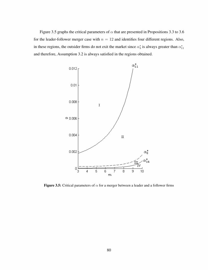
Figure 3.5 graphs the critical parameters of α that are presented in Propositions 3.3 to 3.6

for the leader-follower merger case with n = 12 and identifies four different regions. Also,

in these regions, the outsider firms do not exit the market since α∗3 is always greater than α∗11

and therefore, Assumption 3.2 is always satisfied in the regions obtained.

Figure 3.5: Critical parameters of α for a merger between a leader and a follower firms

80

Chapter 4

Uncertain Efficiency Gains and Merger

Policy

1

4.1 Introduction

The assessment of the efficiency gains resulting from a merger usually raises an information

issue for antitrust authorities. Although some mergers can actually generate significant effi-

ciency gains, these are usually difficult to measure and verify. In practice, it is often the case

that both the firms and the antitrust authority (henceforth, AA) cannot predict exactly the

post-merger efficiency gains, implying that they are not aware of all the conditions they are

going to face after the merger. Sometimes, only after the merger firms and antitrust authorities

will understand the true level of induced efficiency gains. For instance, some pharmaceutical

firms may adopt merger decisions without knowing whether their R&D efforts will be suc-

1This chapter benefited a lot from the seminar participants’ comments at the 8th Annual Meeting of the

Portuguese Economic Journal, University of Minho, School of Economics and Management and at the 10th

Seminar Day of the Doctoral Programme in Economics, Faculty of Economics of University of Porto, 2014.

Also, we are very grateful to Professors Joana Pinho, Joao Correia da Silva, Ricardo Ribeiro and Helder Valente

for their helpful comments and suggestions that substantially improved this paper.

81

cessful or not. Also, any type of firms’ investment could generate uncertainty about future

costs and, sometimes, a merger could actually occur before the uncertainty is resolved.

In 1996, Ciba-Geigy AG (hereinafter “Ciba”) and Sandoz AG (hereinafter “Sandoz”)

proposed a merger to the European Commission (EC). Ciba and Sandoz, two Swiss manu-

facturers, were involved in the research, development and production of biological and chem-

ical products, as well as in the production and marketing of pharmaceutical products. The

merger would create a new enterprise, Novartis AG (hereinafter “Novartis”), that would be

the world’s second largest supplier of pharmaceutical products. This merger raised important

issues regarding the effects on future innovation for the EC and the Federal Trade Commis-

sion (FTC). The EC was first concerned on whether this merger would lead to a decrease of

competition in the market but also on the effects of these two firms combining their R&D

programmes into one single firm. The EC concluded that Novartis would succeed in keeping

its research expenditure lower, in relative terms, than that of its competitors, maintaining its

position as market leader. Nonetheless, the EC concluded that all the Novartis’s competi-

tors have the “critical size” necessary for effective R&D activity and that increases in market

share would be insignificant in most areas. Further, the real possibility of market entry and

the restraining effect of generic pharmaceuticals on pricing were also seen as helping to pre-

vent anticompetitive effects. Both EC and FTC were mainly concerned on the possibility that

this merger would generate adverse effects on market power however, little reference was

made to the merger’s efficiency effects (EC, 1996).

The analysis of merger-induced efficiencies was introduced into the US Horizontal Merger

Guidelines in 1997 (DOJ and FTC, Section 10) and into the European Merger Guidelines in

2004 (EC Horizontal Merger Guidelines, 2004/03, Article 7). The US merger guidelines state

that “Other efficiencies, such as those relating to research and development, are potentially

substantial but are generally less susceptible to verification and may be the result of anticom-

petitive output reductions”. Also, in the European merger guideline the “efficiency defence”

argument has been specifically ruled out and the effects on technical and economic progress

can only be taken into account “provided it is to the consumers’ advantage and does not form

an obstacle to competition”. The significance of potential welfare benefits from innovation

82

or mergers’ induced efficiency gains means it is important to give appropriate weight to this

aspect of competition in merger analysis. Both EU and US merger guidelines allow future

R&D efficiency gains to be taken into account, however these dynamic effects of mergers

are generally disregarded since they are not only difficult to verify and quantify but also very

hard to predict when the AAs are deciding on a merger case.

The purpose of this paper is to contribute to the literature that studies the efficiency gains’

role in merger decisions, departing from a deterministic environment by considering a set-

ting in which there is (symmetric) uncertainty. In particular, we assume that the decisions

of the antitrust authority, when evaluating a merger case, crucially depend on the uncertainty

regarding the efficiency gains realization. In the proposed model, firms and the AA are un-

certain about the level of efficiency gains and, therefore, this uncertainty is going to influence

the decision of the AA but also firms’ incentives to merge. This analysis is useful to the AA

in order to more properly evaluate merger proposals when there is uncertainty about the cost

savings that mergers may induce or not.2

In the absence of uncertainty and in a context of symmetric Cournot oligopoly with linear

demand and costs, a merger is profitable if it comprises a pre-merger market share of at least

80% (Salant et al., 1983; Perry and Porter, 1985). Also, when both firms and the AA are

perfectly informed about the merger induced efficiency gains, the antitrust authority usually

allows the merger when there are important efficiency gains that would lead to lower prices

(Motta and Vasconcelos, 2005; Vasconcelos, 2010).

The present paper is related to two strands of literature on mergers in a Cournot frame-

work: (i) the studies of antitrust authority’s merger decisions, where the AA evaluates the

welfare effects of mergers and allows for merger remedies under uncertainty, such as Cosnita

and Tropeano (2009), Besanko and Spulber (1993), Corchon and Faulı-Oller (2004); and (ii)

works that, investigating the impact of uncertainty on the incentives to merge, conclude that

the incentives to merge depend on the information structure, such as Gal-Or (1988), Sten-

backa (1991), Wong and Tse (1997), Stennek (2003), Qiu and Zhou (2006), Banal-Estanol

(2007), Zhou (2008a,b), Amir et al. (2009). Uncertainty can also be seen as an information

2See Morgan (2001) for the discussion about the significance of reviewing merger cases with uncertainty.

83

sharing problem, for instance, firms can have more information about their own costs than

the AA. Previous contributions to the literature on information sharing among oligopolists

did not consider the possibility of mergers among firms nor AA intervention. In most of

the papers, it is assumed that there is market uncertainty because the marginal cost and/or

the market demand are unknown to the firms, such as, Novshek and Sonnenschein (1982),

Clarke (1983), Sakai (1985), Gal-Or (1985, 1986), Shapiro (1986), Vives (1984, 2002), Li

(1985), Sakai and Yamato (1989), Raith (1996), Lagerlof (2007), Jensen (1992), Elberfeld

and O. Nti (2004), among others.

To our knowledge, however, none of the previous papers has addressed the role of effi-

ciency gains which are uncertain for all players in the merger formation process (firms and

the AA). The present paper then contributes to fill this gap in the extant literature by assuming

that, when firms propose the merger to the AA, all the players (insider, outsiders and AA) are

uncertain about the post-merger efficiency gains and therefore they decide by considering the

expectations on those gains. Once the merger is consummated, both insider and outsider firms

can observe the efficiency gains and compete a la Cournot. This is different from Amir et al.

(2009)’s paper where, after the merger, only the insider firm observes its cost. Our model is

also different from the literature cited before, where it is usually assumed that the merging

firms have an informational advantage, knowing more about the merger induced efficiency

gains than its rivals and the AA. This scenario of “symmetric” uncertainty is probably more

relevant in industries such as electronic communication and ICT markets wherein the pace

of technological progress is impressive. Hence, it becomes very difficult for any player in

the market (the AA or even the merger partners) to predict what will be the merger specific

efficiencies in a context where the competitive snapshot changes very fast and frequently.

Further, our analysis is close to Le Pape and Zhao (2013)’s paper. Le Pape and Zhao (2013)

analyse Stackelberg mergers’ decisions when there is uncertainty on productivity and infor-

mational asymmetry between firms. However, here we focus our analysis on both mergers

and AA decisions, assuming that the firms compete in a Cournot setting and that all firms

have the same degree of uncertainty.

We find that the increase in the degree of uncertainty about merger’s efficiency gains

84

benefits firms (in terms of higher expected profits) and consumers (with higher expected con-

sumer surplus). Further, when the degree of uncertainty is high, there is a greater likelihood

that firms propose a merger to the AA and the AA accepts it. Therefore, uncertainty enhances

both the occurrence of merger proposals and the likelihood that those proposals are cleared

by the AA. We also find that, higher degree of uncertainty increases outsider firms’ incentives

to free-ride on the merger.

The remainder of the paper is organized as follows. In section 4.2 the basic framework

of the model is described. Section 4.3 presents the pre-merger equilibrium results. Section

4.4 analyses the equilibrium of the proposed merger formation game. Also, in this section

we study merger’s free-riding problem. In section 4.5 we present and discuss the obtained

numerical results. Finally, section 4.6 offers some concluding remarks. All the proofs are

relegated to the appendix.

4.2 Basic Framework

We consider a homogeneous good industry with n firms that compete a la Cournot. The

inverse demand function is given by P = 1−Q, where Q =n∑i=1

qi is the aggregate output and

qi is the quantity produced by firm i ∈ {1, ..., n}.

Let ki denote firm i’s capital holdings, where ki ∈ {1, 2, ..., K}. The cost function of a

firm i, which owns ki units of he industry capital and produces qi units of output, is given

by:3

C(αj, qi, ki) =αjK

kiqi,

where K is the total capital in the industry, Σiki = K, that is fixed and αj measures the

endogenous efficiency gains, with αj ≥ 0.4

3This is a simplified version of the cost structure proposed by Motta and Vasconcelos (2005) and captures

also the specific case studied in Horn and Persson (2001). This cost function is based on the one proposed by

Perry and Porter (1985). In their framework firms’ marginal cost is linear in output and mergers reduce variable

costs.4Efficiency gains may result from firm’s combined ability to exploit economies of scale or raise larger

85

In the next sections we analyse the results before the merger, where the efficiency gains

are known with certainty. We then discuss the results obtained after the merger, for both AA

and merger decisions, in a context where there is uncertainty about merger induced efficiency

gains.

4.3 Pre-Merger equilibrium

Before the merger (BM), we assume that firms are symmetric and that each firm owns one

unit of capital, that is, ki = 1. Also, each firm knows, with certainty, its level of efficiency

gains and therefore αi = α, where α is the common efficiency level of all firms before the

merger.

The equilibrium profits and consumer surplus are then given by:

πBMi =(1− nα)2

(n+ 1)2 ,where i = 1, .., n. (4.1)

CSBM =n2 (1− nα)2

2 (n+ 1)2 . (4.2)

Assumption 4.1. Assume that α < 1n

.

The previous assumption is imposed in order to exclude the case in which firms in the

industry do not produce (are inactive) in the pre-merger equilibrium.

4.4 Merger Analysis

In this section we analyse both the AA’s and firms’ merger decision, in a setting where all

firms in the industry and the AA are uncertain over the merger induced efficiency gains.

Assume that, at the status quo industry, one firm in the industry is randomly selected and

has the opportunity to propose, to the AA, a merger involving m ≥ 2 firms. This firm may

amounts of capital, but also from complementarity between technological or administrative capabilities of firms

(Roller et al., 2001).

86

propose a merger with all or a subset of its rivals. Since each firm operates with a constant

marginal cost of production, but the level of its marginal cost is a decreasing function of its

capital holdings, the resultant merged firm becomes more efficient than outsiders by having

ki = m units of assets. We assume that m is given exogenously. Hence, the merger brings

the capital of merging parties into a single larger firm and, therefore, gives rise to endogenous

efficiency gains by decreasing the marginal cost. The level of these potential efficiency gains

is captured by the parameter αi.

When the level of efficiency gains is the same before and after the merger (αi = α),

all firms and the AA know with certainty what will be the merger’s cost savings. Hence,

the higher is the value of α, the stronger the efficiency gains induced by a merger are, and

therefore, the higher is the cost reduction after the merger (Motta and Vasconcelos, 2005;

Vasconcelos, 2010).

However, in our model, the merger also brings uncertainty about the induced efficiency

gains, that is, all firms (insiders and outsiders) and the AA cannot predict precisely the level

of the future merger-induced efficiency gains. Thus, we assume that all players are uncertain

on what will be the exact value of the efficiency gains level, as measured by αi = αu. This

level of future efficiency gains, αu, could be higher, lower or equal than the level of efficiency

gains before the merger, given by α. Therefore the merger effects on firms costs depends both

on the value of α and of the change on the capital holding. If αu is equal to α then, after the

merger, the merged firm knows that it is endowed with the capital of the merging parties

and therefore its cost will decrease. In this case, the outsider firm’s cost will not change. If

αu is lower than α, the insider firms’ cost will decrease due to the increase in capital and

also due to the lower value of α. In this case the outsider firms’ cost will decrease after the

merger. Different results are obtained when αu is higher than α: if αu = kα, then the insider

firm’s cost will remain the same as before the merger however, the outsider firms’ costs will

increase; if αu > kα both insider and outsider firms’ costs increase after the merger; and if

αu < kα then, after the merger, the insider firm’s cost decrease and the outsider firms’ costs

increase.

87

Assumption 4.2. Let αu be a random variable distributed over [0, 12n

].

By assuming that αu < 12n

, we are excluding the case where outsiders exit the market after

the merger takes place.5 The expected value of the efficiency gains in the future is denoted

by E (αu) = µ, where µ ∈ [0, 12n

], and the variance is denoted by V (αu) = σ2 > 0. The σ2

represents the degree of uncertainty and captures the efficiency gains fluctuation. The higher

is σ2, the greater is the uncertainty about the merger’s efficiency gains.

Firm i has to decide whether or not to merge and the AA has to decide whether or not to

accept the proposed merged, both without knowing the actual cost of the merged firm in the

future. We assume that firms set output decisions after uncertainty is solved, given that we

want to study the effects of uncertainty on the decisions of both merger firms and the AA.

We assume that firms are risk neutral and therefore firms’ decisions regarding the merger

are based on the expected values of their profits.6

We also assume that the AA is risk neutral, and that its decision is based on the expected

value of consumer surplus. We consider that the AA’s decision is based on expected consumer

surplus instead on social welfare and, thus, the AA approves the merger if the expected

consumer surplus increases.7 Thus, the private incentives to merge and the AA decisions are

based on expected values.

We model the interactions between the antitrust authority and the merging firms as a

5Exit inducing mergers are rare. Relaxing this would complicate our analysis, since we would have to

consider not only growth by mergers but also growth by capital accumulation.6Note that if we assume that firms’ are risk averse, the utility function of profit for each firm would be given,

for instance, by the following constant absolute risk aversion function u(w) = 1− exp(aw) where a > 0 is the

coefficient of absolute risk aversion. Given that the price is P , the costs are c and that the firm chooses an output

q to maximize the expected utility of profit: E(π) = 12 (1 − exp(a(P − c)q)) + 1

2 (1 − exp(a(P − 1 − c)q)).

This function is concave in q and in our model, the profit is linear in q.7By assuming that the AA evaluates mergers according to a consumer surplus standard this does not mean

that this is always better than the total welfare standard. However, as Lyons (2002) argued, the consumer

surplus standard is applied in most antitrust jurisdictions. Other papers also study how the AA should apply the

consumer surplus standard when challenging a merger, such as Besanko and Spulber (1993), Neven and Roller

(2005), Vasconcelos (2010), Nocke and Whinston (2010), Jovanovic and Wey (2012), among others.

88

four-stage game, with the following timing:

• Stage 1: Firms have to decide whether or not to propose a merger to the AA.

• Stage 2: The AA decides whether or not to accept the proposed merger.

• Stage 3: Nature chooses αu and reveals it to all players.

• Stage 4: Insider and outsider firms choose quantities competing in the usual Cournot

fashion.

In what follows, we will solve the model by following the usual backward induction

procedure.

4.4.1 Product Market Competition

The results presented below refer to the Cournot-Nash equilibrium after the merger (AM),

where firms know the level of efficiency gains (since uncertainty has been resolved in the

previous stage of the game).

In the fourth-stage of the game, firms have already observed the actual value of αu so, they

choose to produce the quantities that maximize their profits. The Cournot equilibrium profits

of insider firm (I) and outsider firms (O) and the consumer surplus (CS) are, respectively,

given by:

πAMI =[ m− nαu ((m− 1) (m− n) + 1)]2

m2 (n−m+ 2)2 (4.3)

πAMO =[ m− nαu (2m− 1)]2

m2 (n−m+ 2)2 (4.4)

CSAM =[ m (n−m+ 1)− nαu (m (n−m) + 1)]2

2m2 (n−m+ 2)2 . (4.5)

As we can observe from equations (4.3), (4.4) and (4.5), without uncertainty about the

level of efficiency gains, both profits and consumer surplus increase with the level of effi-

ciency gains.

Under uncertainty, outsider firms would exit the market if they expected to produce zero

in equilibrium, that is, if µ ≥ mn(2m−1)

. If the expected efficiency gains from merger are very

89

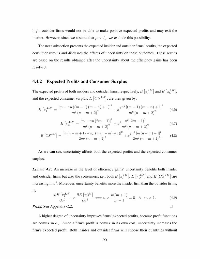
high, outsider firms would not be able to make positive expected profits and may exit the

market. However, since we assume that µ < 12n

, we exclude this possibility.

The next subsection presents the expected insider and outsider firms’ profits, the expected

consumer surplus and discusses the effects of uncertainty on these outcomes. These results

are based on the results obtained after the uncertainty about the efficiency gains has been

resolved.

4.4.2 Expected Profits and Consumer Surplus

The expected profits of both insiders and outsider firms, respectively, E[πAMI

]andE

[πAMO

],

and the expected consumer surplus, E[CSAM

], are then given by:

E[πAMI

]=

[m− nµ ((m− 1) (m− n) + 1)]2

m2 (n−m+ 2)2 + σ2n2 [(m− 1) (m− n) + 1]2

m2 (n−m+ 2)2 (4.6)

E[πAMO

]=

[m− nµ (2m− 1)]2

m2 (n−m+ 2)2 + σ2 n2 (2m− 1)2

m2 (n−m+ 2)2 (4.7)

E[CSAM

]=

[m (n−m+ 1)− nµ (m (n−m) + 1)]2

2m2 (n−m+ 2)2 + σ2n2 [m (n−m) + 1]2

2m2 (n−m+ 2)2 (4.8)

As we can see, uncertainty affects both the expected profits and the expected consumer

surplus.

Lemma 4.1: An increase in the level of efficiency gains’ uncertainty benefits both insider

and outsider firms but also the consumers, i.e., both E[πAMI

], E[πAMO

]and E

[CSAM

]are

increasing in σ2. Moreover, uncertainty benefits more the insider firm than the outsider firms,

if:∂E[πAMI

]∂σ2

>∂E[πAMO

]∂σ2

⇐⇒ n >m(m+ 1)

m− 1≡ n ∧ m > 1. (4.9)

Proof. See Appendix C.2. �

A higher degree of uncertainty improves firms’ expected profits, because profit functions

are convex in αu. Since a firm’s profit is convex in its own cost, uncertainty increases the

firm’s expected profit. Both insider and outsider firms will choose their quantities without

90

knowing the exact value of the costs.8 The insider firm expects that, after the merger, the

cost is going to decrease due to the synergies generated, that is, due to an increase in the

capital stock of the merged firm. However, the insider firm does not know how much is this

cost saving, since the insider firm’s cost decreases in three different scenarios: (i) αu < α,

(ii) αu = α and (iii) α < αu < kα. Since the insider firm expects a lower cost, it knows

that, even without uncertainty, the resultant firm is going to produce a large quantity. The

uncertainty about how much the cost reduces also affects the outsider firms. Although each

outsider firm still has one unit of capital, if the cost saving is very high, we know that, without

uncertainty, outsiders will respond by reducing quantity. However, under uncertainty, only if

αu is smaller than α, there will also be significant cost savings for outsider firms and this will

increase both quantities and profits of all outsider firms. If this is the case, the expected net

effect is an increase in the total quantity and a decrease in the total price (which also happens

without uncertainty).

Without uncertainty and cost synergies, mergers usually lead to a sharp reduction of the

total output. As consequence, in deterministic models, mergers usually reduce the consumer

surplus. However, when there are cost synergies, the reverse can actually occur even without

uncertainty. In our model, the higher is the uncertainty about the cost synergies generated

by the merger, the larger the value of σ2 and the greater the expected consumer surplus

will be. After the merger, both the insider and outsider firms expect to benefit from cost

synergies if αu is smaller than α and, therefore, expect to increase the quantities produced.

However, it may happen that, after the merger, αu is greater than α and, therefore, the insider

firm’s cost decreases but the outsider firms’ cost increase. In this case, the insider firm still

produces more quantity but the outsider firms’ will respond by producing a lower quantity.

Nevertheless, under uncertainty, both insider and outsider firms do not adjust so sharply their

production. Consequently, the net effect is an increase in the total quantity in the market,

which affects positively the consumer surplus. Hence, both profits and consumer surplus are

increasing functions with respect to the uncertainty parameter, σ2.

Additionally, under uncertainty, the profits of the insider and outsider firms are affected

8This is a similar result as obtained by Zhou (2008a)’s paper.

91

differently. More precisely, if the number of firms in the market is higher than a threshold

n, uncertainty has a higher effect on insider firm’s profits than on outsiders. However, if the

number of firms in the market is lower than n, the reverse occurs. If we solve with respect

to m we would get that (n−1)−√

((n−1)3−4n)

3< m <

(n−1)+√

((n−1)3−4n)

3, that is when the

number of insider firms is greater than 50% of the firms in the market usually the impact of

uncertainty on outsiders profits is greater than the impact of uncertainty on insider’s profit.

Further, the extent of the uncertainty effect on both expected profits and consumer surplus

is shown to depend on the number of firms in the market (n) and on the number of firms

involved in the merger (m). The higher is the number of firms in the market, the higher the

positive impact of uncertainty on consumer surplus and on insider profits is, but the lower

the positive impact on outsider profits is. Also, the higher is the number of insider firms,

the larger the positive effect of uncertainty on (insider and outsider) profits and on consumer

surplus is. However, from numerical simulation, we have seen that as the number of insider

firms increases, that is, when insiders involve more than 50% of the firms in the market,

uncertainty begins to have a lower but still positive effect on both consumer surplus and

insider profits. Hence, in order for the merger to be profitable, the insider firm must compete

with a sufficiently high number of outsider firms.9

Lemma 4.2: If:

(i) m = n (full merger), both expected consumer surplus and insider profits always de-

crease with the expected mean over the efficiency gains level;

(ii) m < n (partial merger), the expected outsider profits and the expected consumer sur-

plus decrease with the level of expectations over the efficiency gains, however the ex-

pected insider profits increase if those expectations satisfy the following threshold:

µ > mn[(m−n)(m−1)+1]

.


9For instance, if there are n = 11 firms in the market, in order for the merger between two or three firms

(m = 2, 3) to be profitable, it is necessary to exist at least five outsider firms.

92

Lemma 4.2 states that, after the merger, the expected outsider firms’ profits and the ex-

pected consumer surplus decrease with the expected mean over the efficiency gains (µ). If

the expectations over the efficiency gains are very high this could mean that, after the merger,

outsider firms would have incentives to exit the market since their profits would become neg-

ative. Hence, the insider firm would have higher market power, which would negatively affect

the consumer surplus. Also, the expected insider firms’ profits increase if the expectations

over the efficiency gains are sufficiently high and if the merger does not involve all the firms

in the market.

Before looking at the results obtained to the AA decision, we assume the following:10

Assumption 4.3. Assume that µ = α.

Assumption 4.3 states that the expected efficiency gains level are equal to the benchmark

firm’s efficiency gains level, that is, the efficiency gains level of both insider and outsider

firms at the status quo industry. After the merger, the insider firm expects that its cost is

going to reduce, since now only one firm encompasses all capital assets of the merging firms.

However, the insider firm does not know how much is this reduction. Therefore, for simplic-

ity, we assume that the expectations on the level of efficiency gains are rational and equal to

the efficiency gains before the merger. Hence, the merged firm expects the cost reduction to

only depend on the level of capital of the merging parties. This assumption allows us isolate

the effects of uncertainty on both AA’s and firms’ merger decisions. By assuming µ = α the

interpretation of the results is the same as before: the higher is α, the stronger the efficiency

gains induced from the merger are.

Recall that we are only considering the scenario in which outsider firms do not exit the

market after the merger. Hence, after the merger the market structure consists of n −m + 1

firms: n−m outsiders with one unit of capital and one firm with k = m units of capital.11

10This assumption is not crucial. Actually, we obtain our main results without assuming it, but, in order to

present clear expressions we need to impose it. See Appendix C.3 for further information on the results obtained

without Assumption 4.3.11However, we do not exclude the case where the merger involves all the firms in the industry. See Appendix

93

In what follows, both AA and merging firms decisions are made under uncertainty.

4.4.3 Antitrust Authority’s Decision

The AA decides whether to allow or block any proposed merger. The AA accepts the merger

if the expected consumer surplus after the merger is greater or equal than the consumer sur-

plus before the merger (E[CSAM

]≥ CSBM ).

Proposition 4.1. The AA will accept the merger if E[CSAM

]− CSBM > 0, i.e. iff:

σ2 ≥ σ2AA{m,n−m,α} ≡

m2 (n−m+ 2)2 n2 (1− nα)2 − [m (n−m+ 1)− nα (m (n−m) + 1)]2 (n+ 1)2

(n+ 1)2 n2 [m (n−m) + 1]2.

(4.10)


Proposition 4.1 states that when uncertainty is high, there is a greater likelihood that the

AA accepts the merger. Since the consumer surplus before the merger (whose expression is

given in (4.2)) does not depend on the uncertainty parameter, the higher is the uncertainty,

σ2, the greater is the expected consumer surplus after the merger. Consequently, when un-

certainty is high, the expected consumer surplus variation also increases. Further, when the

level of efficiency gains or the number of insider firms increases, σ2AA{m,n−m,α} decreases.

This means that the interval of uncertainty level above which the AA accepts the merger in-

creases. This happens because the difference between the consumer surplus before and after

the merger increases. The reverse occurs when the number of firms increases.

When there are cost synergies, mergers can improve consumer surplus by increasing out-

put. This improvement could actually be higher when there is uncertainty about cost syn-

ergies. Also, since those firms that propose the merger to the AA are the ones that usually

have more certainty about their future cost savings, this could actually work as a signal to the

AA. If this is a good signal, the AA could easily identify the type of firms that will generate

greater cost synergies and , therefore, there is a greater likelihood that the merger proposal by

this type of firms ends up being accepted by the AA. This being the case, under uncertainty

C.1.4. for further information on full merger results.

94

there is a greater likelihood that the merger is accepted by the AA.

4.4.4 Merger Decision

In this section, we examine firms incentives to merge. Firms decisions on whether to merge

or not result from the comparison between the expected profits of the merged firm with the

profits before the merger. Hence, the merger profitability condition depends on the expected

profits of the merged firm, that is, firms will propose the merger if E[πAMI

]≥ mπBM .

Proposition 4.2. If the level of uncertainty is sufficiently high, there is a greater likelihood

that firms propose a merger. Firms will propose the merger if they anticipate that it will be

profitable, i.e. iff:12

σ2 ≥ σ2MP{m,n−m,α} ≡

(1− nα)2m3 (n−m+ 2)2 − [m− nα ((m− 1) (m− n) + 1)]2 (n+ 1)2

(n+ 1)2 n2 [(m− 1) (m− n) + 1]2.

(4.11)


From Proposition 4.2, we conclude that uncertainty promotes the expected merger prof-

itability. As the extent of the variance exceeds a certain threshold (σ2MP{m,n−m,α}) the ex-

pected profit of the merged firm becomes larger than the sum of the firm’s profits in the

benchmark case, and firms that face cost uncertainty choose to merge. Further, when the

number of insider firms increases, the region of uncertainty above which the merger is prof-

itable increases (∂σ2MP{m,n−m,α}

∂m< 0), hence the profits after the merger exceed those before

the merger and firms have more incentives to propose the merger. In the deterministic model,

without efficiency gains, unless the merger involves a sufficient number of insiders, most

of the horizontal mergers are unprofitable (Salant et al., 1983). However, in our model, as

the uncertainty increases, the expected profit also increases because the gain of the optimal

quantity adjustment increases, and therefore it is possible that the expected profit of insider

firm (as measured by (4.6)) exceeds the sum of profits of the pre-merger firms (whose ex-

12Note that n > 3, otherwise insider firm’s profit would not depend on the σ2 parameter and therefore this

expression would not exist.

95

pression is given in (4.1)). Hence, the insider firm has a higher profit both directly from the

cost advantage and indirectly from the favourable responses from outsider firms. Since the

pre-merger profits are not affected by uncertainty, it is expected that the merger becomes at

least more profitable than in the deterministic models.

As the degree of uncertainty becomes larger, firms have more incentives to merge and

therefore, we conclude that cost uncertainty is able to induce the firms to merge. This re-

lationship between merger profitability and cost uncertainty is also investigated by Banal-

Estanol (2007) and Zhou (2008a,b). The results obtained in these papers are similar to ours

however, our framework is different from the adopted by these authors since we assume that

all players face the same level of uncertainty. For instance, Banal-Estanol (2007) consid-

ers that firms face idiosyncratic uncertainty about costs and that uncertainty generates an

informational advantage only to the merging firms, increasing merger profitability. Also, dif-

ferently from our paper, Zhou (2008a,b) assumes that after the merger, costs are realized and

each firm learns its own costs but not the costs of its rivals. Zhou (2008a,b) argues that when

costs are uncertain and firms choose quantities before the uncertainty is resolved, a merger

is more profitable the greater the uncertainty. Zhou (2008a,b) shows that firm’s incentives to

merge are enhanced by production rationalization.13

4.4.5 Free-riding Problem

In this subsection we study the effects of uncertain efficiency gains on merger’s free-riding

problem.

In the deterministic models, mergers face a free-riding problem, given that outsider firms

are the ones that benefit most from the merger (free-riding problem). In order to assess if

there is a free-riding problem in our model, we compare the expected profit of the merged

firm with the expected profits of outsiders.

13We could extend our analysis in order to allow for differences in the uncertainty level among all the players.

We realize that this is an important subject for further research and that this far behind the scope of the present

paper.

96

Proposition 4.3. There is a free-riding problem if E[πAMI

]< mE

[πAMO

], i.e., iff:

σ2 > σ2fr{m,n−m,α} ≡

m (m− 1) [2nα (m+ n+ 1)−m]

mn2 (2m− 1)2 − n2 [(m− 1) (m− n) + 1]2− α2 (4.12)


Proposition 4.3 states that, if the uncertainty over merger’s efficiency gains is high, out-

sider firms benefit more from the merger than the insider firms. Hence, an increase in the

level uncertainty promotes merger’s free-riding problem. After the merger, the merged firm

expects to produce more quantity than each outsider firm, due to the synergies generated. The

outsider firms’ production depends on whether αu is greater, equal or lower than α. If the

level of expected efficiency gains increases and becomes higher than α after the merger, the

insider firm still produces more quantity but the outsider firms’ will respond by producing a

lower quantity. While the profit of the insider firm always increases with the uncertainty, that

of an excluded rival also increases as a result of the merger. For high degree of uncertainty,

firms would prefer to wait for their rivals to merge and, thus, benefit from the merger.

Lemma 4.3. Keeping the number of firms constant (n), as the number of insider increases

(m), the region of uncertainty level below which there is no free-riding decreases, i.e.,∂σ2fr

∂m>

0. Also, keeping the number of insiders constant, an increase in the number of firms in the

market, increases the region of uncertainty level below which there is no free-riding, i.e.,∂σ2fr

∂n< 0.

We find that, under uncertainty about cost synergies and keeping the number of firms

constant, as the number of insider firms increases, firms have more incentives to deviate and

to compete against its rivals as an outsider. Also, keeping the number of insiders constant, as

the number of firms in the market increases, outsider firms have less incentives to free-ride

on the merger.

97

4.5 Numerical Application

In what follows, assume that the total quantity of capital available in the industry is equal to

four units (K = 4) and that this capital is equally distributed amongst four firms (n = 4) in

the status quo industry structure.

We analyse the results obtained for both firms and AA decisions for three cases:

1) Merger involving two firms (m = 2);

2) Merger involving three firms (m = 3); and

3) Merger to monopoly (m = 4).

Again, we restrict our attention to the case in which, after the merger, outsiders do not

exit the market (αu < 18). Further, we also analyse if there is a free-riding problem for both

cases 1 and 2.

The following result sums up the AA decisions for the three merger cases.

Result 4.1.

• The AA accepts the merger involving two firms (case 1) if: σ2 ≥ σ2AA{2,1,1,α};

• The AA accepts the merger involving three firms (case 2) if: σ2 ≥ σ2AA{3,1,α};

• The AA accepts the merger to monopoly (case 3) if: σ2 ≥ σ2AA{4,α}.


The following result sums up firms decisions for the three merger cases.

Result 4.2.

• Firms will propose a merger involving two firms (case 1) if: σ2 ≥ σ2MP{2,1,1,α};

• Firms will propose a merger involving three firms (case 2) if: σ2 ≥ σ2MP{3,1,α};

• Firms will propose a merger to monopoly (case 3) if: σ2 ≥ σ2MP{4,α}.


The following result sums up the results obtained for the free-riding problem for the first

two merger cases.

98

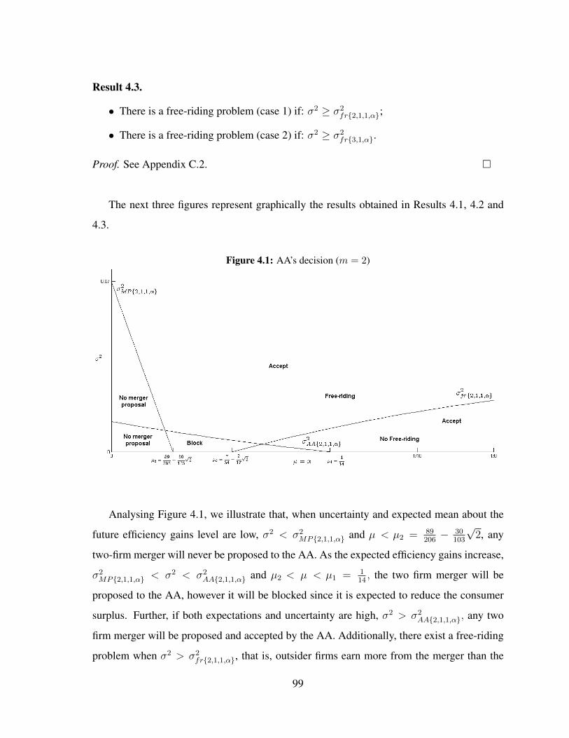
Result 4.3.

• There is a free-riding problem (case 1) if: σ2 ≥ σ2fr{2,1,1,α};

• There is a free-riding problem (case 2) if: σ2 ≥ σ2fr{3,1,α}.


The next three figures represent graphically the results obtained in Results 4.1, 4.2 and

4.3.

Figure 4.1: AA’s decision (m = 2)

Analysing Figure 4.1, we illustrate that, when uncertainty and expected mean about the

future efficiency gains level are low, σ2 < σ2MP{2,1,1,α} and µ < µ2 = 89

206− 30

103

√2, any

two-firm merger will never be proposed to the AA. As the expected efficiency gains increase,

σ2MP{2,1,1,α} < σ2 < σ2

AA{2,1,1,α} and µ2 < µ < µ1 = 114, the two firm merger will be

proposed to the AA, however it will be blocked since it is expected to reduce the consumer

surplus. Further, if both expectations and uncertainty are high, σ2 > σ2AA{2,1,1,α}, any two

firm merger will be proposed and accepted by the AA. Additionally, there exist a free-riding

problem when σ2 > σ2fr{2,1,1,α}, that is, outsider firms earn more from the merger than the

99

insider firms and this could promote the free-riding. Also, if the expected efficiency gains are

higher than µ3 = 734− 2

17

√2 and if uncertainty is not very high σ2 < σ2

fr{2,1,1,α} there is a

possibility that the merger is accepted by the AA and there is no free-riding problem.


Figure 4.2 summarizes the results obtained when the merger involves three firms. We can

observe that when both expected efficiency gains and uncertainty are low, σ2 < σ2MP{3,1,α},

µ < µ5 = 159436− 45

218

√3, any three-firm merger will never be proposed to the AA. As the

expected efficiency gains increase, σ2MP{3,1,α} < σ2 < σ2

AA{3,1,α} and µ < µ4 = 332

, any

three-firm merger proposal will be proposed and blocked by the AA. However, when both

the expected efficiency gains and the uncertainty increase, σ2 > σ2AA{3,1,α} and µ4 < µ < 3

32,

the three-firm merger will always be proposed and accepted by the AA. Further, in this case

there is also a free-riding problem when σ2 > σ2fr{3,1,α}, that is, the only outsider firm earns

more from the merger than the insider firms and this could also promote merger’s free-riding

problem. Also, if the expected efficiency gains are higher than µ6 = 637− 9

148

√3 and if

uncertainty is not very high σ2 < σ2fr{3,1,α} there is a greater likelihood that the merger of

three firms is accepted by the AA and outsiders have no incentives to free ride on it.

100


The results obtained for the full merger case are illustrated in Figure 4.3. Since the

σ2MP{4,α} is always negative, for any level of uncertainty, the firms have always incentive

to propose a merger to monopoly. However, if the expected efficiency gains and uncertainty

are low, σ2 < σ2AA{4,α} and µ < µ7 = 1

9, any merger proposal to monopoly will be blocked

by the AA. As both uncertainty and expected efficiency gains increase, µ > µ7 = 19, and

σ2 > σ2AA{4,α}, the merger to monopoly will always be accepted by the AA.

Figure 4.4 sums up the results obtained for the three merger cases.

101

Figure 4.4: AA’s decision (m = 2, 3, 4)

We conclude that when the level of uncertainty and expected efficiency gains are high, the

firms have incentives to propose any type of merger and this merger has a greater likelihood

of being accepted by the AA. When both levels of uncertainty and expected efficiency gains

are low, the firms have less incentives to propose the merger. As the expected efficiency

gains increase, the firms usually propose the merger in each case, however the AA rejects it

for all or some particular cases. Usually in the models without uncertainty about the future

synergies generated by the merger, the AA only accepts the merger if these efficiency gains

are sufficiently high (Motta and Vasconcelos, 2005; Vasconcelos, 2010). In contrast, the

present paper shows that, with uncertainty, the probability of the merger being accepted is

higher than without uncertainty and, for some cases, mergers could be accepted even if the

expected efficiency gains are intermediate. Finally, as the number of insider firms increases

it is more difficult for the merger to be approved by any AA, even with uncertainty, unless

the expected efficiency gains are very high.

102

4.6 Concluding Remarks

In this paper we investigate the effects of mergers in a context wherein, both firms and the

AA are uncertain about the level of efficiency gains and, therefore, this uncertainty is going

to influence the decision of AA but also firms’ incentives to merge.

In the absence of uncertainty and when firms are symmetric, the merger will not be prof-

itable unless 80% of the firms in the industry are part of the merger. However, we find that,

under uncertainty and asymmetric firms, even when the merged firm is not composed of at

least 80% of the firms in the industry, when the uncertainty increases, the expected profit of

the merged firm exceeds insiders’ pre-merger profits, and therefore firms have incentives to

merge. Moreover, we find that the higher the level of uncertainty in the market regarding

merger induced efficiencies, the higher the expected consumer surplus after the merger. This

then implies that, given the AAs usually base their merger policy decisions on a consumer

welfare standard, higher uncertainty also increases the likelihood that a merger proposal ends

up being approved by the AA. Further, we find that a higher degree of uncertainty promotes

merger’s free-riding problem, by increasing the likelihood that outsider firms benefit more

from the merger than the insider firm.

The framework and the assumptions we have assumed are of a particular kind. It would

be interesting to extend our model to assess the effects on the decisions of all players, when

both firms (insider and outsiders) and the AA face different degrees of uncertainty over the

merger’s cost savings. Also, it would be interesting to study the case where the AA is a

forward looking type and expects that the first merger is followed by a defensive merger. We

think that this is a very important subject for further research.

103

Appendix

Appendix C.1. Model derivations

C.1.1. Pre-Merger equilibrium

Before the merger, firms decide individually their quantity. Knowing that firms are sym-

metric and that each firm owns one unit of asset, the quantity produced by each firm is given

by: qi = 1−nα(n+1)

, with i = 1, .., n. Therefore, the total quantity and price are respectively given

by Q = n 1−nα(n+1)

and PBM = 1+n2αn+1

. The profit and the consumer surplus are then given by:

πBMi = (1−nα)2

(n+1)2 and CSBM = 12n2(1−nα)2

(n+1)2 .

C.1.2. Post-Merger equilibrium

After the merger of m firms, insider firm now owns m units of capital while the out-

siders still own 1 unit of capital. Then the merged firm will produce, in equilibrium, QI =

m−nαu((m−1)(m−n)+1)m(n−m+2)

and the outsiders will produce qo = m−nαu(2m−1)m(n−m+2)

.

The equilibrium profits are then given by:

πAMI = [ m−nαu((m−1)(m−n)+1)]2

m2(n−m+2)2 and πAMO = [ m−nαu(2m−1)]2

m2(n−m+2)2 .

If we study the sign of the derivatives of the profits with respect to αu, n and m, we get:∂πAMI∂αu

> 0 if αu > mn((m−1)(m−n)+1)

, which is always true.∂πAMI∂m

> 0, for all αu.∂πAMI∂n

> 0, always positive if αu is sufficiently high, that is, if

αu >m

2n(3m−2)−m(2mn+3)+m2(m−3)+n2(m−1)+2.

∂πAMO∂αu

> 0 if αu > mn(2m−1)

, which is always true.∂πAMO∂m

> 0 this is true for αu > mn(2m−1)

and αu < m2

n(2m(m−1)+n+2).

∂πAMO∂n

> 0, which is always true.

The consumer surplus (CS) is then given by:

CSAM = [m(n−m+1)−nαu(m(n−m)+1)]2

2m2(n−m+2)2 .

If we study the sign of the derivatives of the consumer surplus with respect to αu, n and

104

m, we get:∂CSAM

∂αu> 0 if αu >

m(n−m+1)n(m(n−m)+1)

∂CSAM

∂m> 0 if m2

n(n+2m(m−1)+2)< αu <

m(n−m+1)n(m(n−m)+1)

∂CSAM

∂n> 0 if αu >

m(n−m+1)n(m(n−m)+1)

∪ αu < mm(−2m(n+1)+n(n+4)+m2−1)+2

C.1.3. Expected Insider and Outsider Profits and Expected Consumer Surplus

Applying the expectations on equation (4.3), we obtain equation (4.6):

E[πAMI

]= E

[m2 − 2mnαu ((m− 1) (m− n) + 1) + n2α2

u ((m− 1) (m− n) + 1)2

m2 (n−m+ 2)2

]

=m2 − 2mnE (αu) ((m− 1) (m− n) + 1) + n2E (α2

u) ((m− 1) (m− n) + 1)2

m2 (n−m+ 2)2 .

Knowing that V (αu) = E (α2u)−E2 (αu) and that E (αu) = µ and V (αu) = σ2 we get

that:

E[πAMI

]=

m2 − 2mnµ ((m− 1) (m− n) + 1) + n2 (σ2 + µ2) ((m− 1) (m− n) + 1)2

m2 (n−m+ 2)2

=[m− nµ ((m− 1) (m− n) + 1)]2

m2 (n−m+ 2)2 + σ2n2 [(m− 1) (m− n) + 1]2

m2 (n−m+ 2)2 .

Applying the expectations on equation (4.4), we get equation (4.7):

E[πAMO

]= E

[[ m− nαu (2m− 1)]2

m2 (n−m+ 2)2

]= E

[m2 − 2mnαu (2m− 1) + n2α2

iu (2m− 1)2

m2 (n−m+ 2)2

]

=[m− nµ (2m− 1)]2

m2 (n−m+ 2)2 + σ2 n2 (2m− 1)2

m2 (n−m+ 2)2 .

Applying the expectations on equation (4.5) we get equation (4.8):

E[CSAM

]= E

[[ m (n−m+ 1)− nαu (m (n−m) + 1)]2

2m2 (n−m+ 2)2

]

=(m (n−m+ 1)− nµ (m (n−m) + 1))2

2m2 (n−m+ 2)2 + σ2n2(m (n−m) + 1)2

2m2 (n−m+ 2)2 .

105

C.1.4. Full Merger Results

The monopoly (M) profit, price and consumer surplus for Stages 3 and 4 are given by:

πM =

(m− nαu

2m

)2

PM =m+ nαu

2m

CSM =1

2

(m− nαu)2

(2m)2

E[πM]

=m2 − 2mnµ+ n2 (σ2 + µ2)

4m2

E[CSM

]=m2 − 2mnµ+ n2 (σ2 + µ2)

8m2.

Appendix C.2. Proofs

C.2.1. Proof of Lemma 4.1

Deriving E[πAMI

], E[πAMO

]and E

[CSAM

]with respect to the variance, σ2, we obtain:

∂E[πAMI ]∂σ2 = n2((m−1)(m−n)+1)2

m2(n−m+2)2 > 0

∂E[πAMO ]∂σ2 = n2(2m−1)2

m2(n−m+2)2 > 0

∂E[CSAM ]∂σ2 = n2(m(n−m)+1)2

2m2(n−m+2)2 > 0

∂E[πAMI ]∂σ2 − ∂E[πAMO ]

∂σ2 = n2(m−1)[n(m−1)−m(m+1)]m2(n−m+2)

∂E[πAMI ]∂σ2 >

∂E[πAMO ]∂σ2 ⇐⇒ n > m(m+1)

m−1≡ n.

Both E[πAMI

], E[πAMO

]and E

[CSAM

]are increasing with respect to the variance, σ2.

Thus the profits and the consumer surplus increase as the uncertainty grows.

106

�

C.2.2. Proof of Lemma 4.2

Differentiating E[πAMI

], E

[πAMO

]and E

[CSAM

]with respect to µ we find that the

derivatives are positive if and only if:

∂E[πAMI ]∂µ

= −2mn((m−1)(m−n)+1)+2n2µ((m−1)(m−n)+1)2

m2(n−m+2)2 > 0⇔ µ > mn((m−n)(m−1)+1)

.

∂E[πAMO ]∂µ

= −2mn(2m−1)+2n2µ(2m−1)2

m2(n−m+2)2 > 0⇔ µ > mn(2m−1)

.

In the region of parameter values wherein the outsiders are active after the merger, µ <m

n(2m−1), their expected profits always decrease in the level of expected efficiency gains. Oth-

erwise, they will exit the market (and here we assume that all firms are active after the merger

takes place).Hence, when the merger does not involve all the firms in the industry (n > m),

outsiders’ profits could increase with the level of expectations if µ > mn(2m−1)

. However, in

this region outsiders would exit the market. Since we have excluded this scenario, outsiders’

profits always decrease with the µ.

∂E[CSAM ]∂µ

= −2nm(n−m+1)(m(n−m)+1)+2n2µ(m(n−m)+1)2

2m2(n−m+2)2 > 0⇔ µ > m(n−m+1)n(m(n−m)+1)

.

Different results are obtained when the level of expectations is not too high and the merger

does not involve all the firms in the industry (n > m). Both expected insider profits and

expected consumer surplus increase if the expectations satisfy the following thresholds: µ >m

n((m−n)(m−1)+1)and µ > m(n−m+1)

n(m(n−m)+1), respectively. From the numerical simulation we know

that µ > mn((m−n)(m−1)+1)

is always negative and since we assume that µ > 0, hence when the

merger does not involve all the firms in the industry, the expected insiders’ profits increase

with the expected efficiency gains level. However, we also know that µ > m(n−m+1)n(m(n−m)+1)

is

always greater than 12n

. Hence, when the merger does not involve all the firms in the industry,

the expected consumer surplus decreases with the expected efficiency gains level.

Additionally, if the merger involves all the firms in the industry (n = m) both expected

consumer surplus and expected insider profits increase if µ > 1. Since we assume that

107

µ < 12n< 1, therefore both expected consumer surplus and insider profits always decrease

with the level of expectations, when the merger is to monopoly.

�

C.2.3. Proof of Proposition 4.1

Equation (4.10) is obtained from the expression for the expected variation of the consumer

surplus. It is straightforward to show that ∆ECS > 0 holds for σ2 > σ2{m,n−m}. Hence, the

AA will accept the merger if it anticipates it will enhance expected consumer surplus, i.e.,

iff: E[CSAM

]≥ CSBM . This happens when:

∆E[CS] = [m(n−m+1)−nµ(m(n−m)+1)]2

2m2(n−m+2)2 + σ2 n2[m(n−m)+1]2

2m2(n−m+2)2 − 12n2(1−nα)2

(n+1)2 ≥ 0

From Assumption 4.3, we know that α = µ:

[m(n−m+1)−nα(m(n−m)+1)]2

2m2(n−m+2)2 + σ2 n2[m(n−m)+1]2

2m2(n−m+2)2 − 12n2(1−nα)2

(n+1)2 ≥ 0

Solving with respect to σ2, we get:

σ2 ≥ m2(n−m+2)2n2(1−nα)2−[m(n−m+1)−nα(m(n−m)+1)]2(n+1)2

(n+1)2n2[m(n−m)+1]2.

�

Note that:∂σ2AA{m,n−m,α}

∂α< 0

∂σ2AA{m,n−m,α}

∂n< 0

∂σ2AA{m,n−m,α}

∂m> 0.


Firms will propose the merger if: E[πAMI

]≥ mπBM

E[MP ] ≡ [m−nµ((m−1)(m−n)+1)]2

m2(n−m+2)2 + σ2 n2[(m−1)(m−n)+1]2

m2(n−m+2)2 −m (1−nµ)2

(n+1)2 ≥ 0

Solving with respect to σ2 and knowing that µ = α get:

σ2 ≥ (1−nα)2m3(n−m+2)2−[m−nα((m−1)(m−n)+1)]2(n+1)2

(n+1)2n2[(m−1)(m−n)+1]2.

108

�

Note that:∂σ2MP{m,n−m,α}

∂α< 0

∂σ2MP{m,n−m,α}

∂n> 0

∂σ2MP{m,n−m,α}

∂m< 0.


There is a free-riding problem when E[πAMI

]< mE

[πAMO

], that is,

m(

[m−nµ(2m−1)]2

m2(n−m+2)2 + σ2 n2(2m−1)2

m2(n−m+2)2

)−(

[m−nµ((m−1)(m−n)+1)]2

m2(n−m+2)2 + σ2 n2[(m−1)(m−n)+1]2

m2(n−m+2)2

)> 0

Solving with respect to σ2 :

σ2 > m(m−1)[2nα(m+n+1)−m]

mn2(2m−1)2−n2[(m−1)(m−n)+1]2− α2.

�

Note that:∂σ2fr{m,n−m,α}

∂αcould be greater or lower than zero.

∂σ2fr{m,n−m,α}

∂n< 0

∂σ2fr{m,n−m,α}

∂m> 0

C.2.6. Proof of Result 4.1

Replacing n = 4 and m = 2, 3, 4, for each merger case, we get the results for the AA’s

decision in Result 4.1:

• The AA accepts the merger of two firms (case 1) if: σ2 ≥ σ2AA{2,1,1,α} ≡

(14µ−1)(114µ−31)2500

;

• The AA accepts the merger of three firms (case 2) if: σ2 ≥ σ2AA{3,1,α} ≡

(32µ−3)(112µ−33)1600

;

• The AA accepts the merger to monopoly (case 3) if: σ2 ≥ σ2AA{4,α} ≡

3(9µ−1)(37µ−13)25

.

�

109


Replacing n = 4 and m = 2, 3, 4, for each merger case, we get the results for the merger

profitability in Result 4.2:

• Firms will propose a merger of two firms (case 1) if: σ2 ≥ σ2MP{2,1,1,α} ≡

−356µ+412µ2+7100

;

• Firms will propose a merger of three firms (case 2) if: σ2 ≥ σ2MP{3,1,α} ≡

−1272µ+1744µ2+9200

;

• Firms will propose a merger to monopoly (case 3) if: σ2 ≥ σ2MP{4,α} ≡

3(11µ+1)(7µ−3)25

.

�


Replacing n = 4 and m = 2, 3, 4, for each merger case, we get the results for the free-

riding problem in Result 4.3:

• There is a free-riding problem (case 1) if: σ2 ≥ σ2fr{2,1,1,α} ≡ −µ2 + 7

17µ− 1

68;

• There is a free-riding problem (case 2) if: σ2 ≥ σ2fr{3,1,α} ≡ −µ2 + 12

37µ− 9

592.

�

Appendix C.3. Results without Assumption 4.3By Assumption 4.3 we assume that the expectations on the level of efficiency gains are

rational and equal to the efficiency gains before the merger. If we did not consider that µ = α

our results would not change. However, now we would have a three-dimensional analysis of

the results, which would be more complex.

• If µ < mn(2m−1)

, outsiders do not exit (NE) the market, hence the AA will accept the

merger if E[CSAM

]≥ CSBM , that is, if:

∆CSNE =m2(n−m+1)2−2µnm(n−m+1)(m(n−m)+1)+n2(σ2+µ2)(m(n−m)+1)2

2m2(n−m+2)2 − n2(nα−1)2

2(n+1)2 ≥ 0;

σ2 > −n2µ2(m(n−m)+1)2(n+1)2+2µnm(n−m+1)(m(n−m)+1)(n+1)2

n2(m(n−m)+1)2(n+1)2 +

+m2(n2(nα−1)2(n−m+2)2−(n−m+1)2(n+1)2)

n2(m(n−m)+1)2(n+1)2 .

110

∂∆CSNE∂µ

< 0⇔ µ < m(n−m+1)n(m(n−m)+1)

;

∂∆CSNE∂σ2 = 1

2n2 (m(m−n)−1)2

m2(n−m+2)2 .

The higher is the σ2 the greater is the CSAM , the greater the ∆CSNE is.

∂∆CSNE∂α

= n3 1−nα(n+1)2 ;

∂∆CSNE∂α

> 0⇔ α > 1n

, however α must be lower than 1n

, otherwise firms do not produce

before the merger.

• If µ > mn(2m−1)

, then outsider firms will exit the market, hence the AA will accept the

merger if E[CSAM

]≥ CSBM , that is, if:

∆CSE ≡(n+ 1)2m2 −mnµ+ n2 (σ2 + µ2) (n+ 1)2 − 4m2n2 (nα− 1)2

8 (n+ 1)2m2≥ 0.

∂∆CSE∂µ

> 0⇔ µ > m2n(n+1)2 ;

∂∆CSE∂α

= −16m2n4α+16m2n3

2(n+1)28m2 = n3 1−nα(n+1)2 ;

∂∆CSE∂α

> 0⇔ α < 1n

, which is always true.

∂∆CSE∂σ2 = n2(n+1)2

8(n+1)2m2 > 0.

The higher is the σ2 the greater the CSM is and, thus, the greater is ∆CSE . Hence, with

high uncertainty on the level of efficiency gains, the greater is the likelihood that the AA

accepts the merger to monopoly.

• If µ < mn(2m−1)

, outsiders do not leave the market. Hence, firms will propose the merger

if it is profitable, i.e., E[πAMI

]≥ mπBM :

m2−2mnµ((m−1)(m−n)+1)+n2(σ2+µ2)((m−1)(m−n)+1)2

m2(n−m+2)2 ≥ m (1−nα)2

(n+1)2 .

MPNE ≡m2−2mnµ((m−1)(m−n)+1)+n2(σ2+µ2)((m−1)(m−n)+1)2

m2(n−m+2)2 −m (1−nα)2

(n+1)2 ≥ 0.

∂MPNE∂µ

= −2mn((m−1)(m−n)+1)+2n2µ((m−1)(m−n)+1)2

m2(n−m+2)2 .

∂MPNE∂µ

> 0⇔ µ > mn((m−n)(m−1)+1)

(always true).

111

∂MPNE∂α

= 2nm 1−nα(n+1)2 .

∂MPNE∂α

> 0⇔ α < 1n

(always true).

∂MP1

∂σ2 = n2((m−1)(m−n)+1)2

m2(n−m+2)2 > 0.

• If instead, µ > mn(2m−1)

, outsider firms exit the market. Hence, firms will propose the

merger to monopoly if it is profitable:

MPE ≡m2 − 2mnµ+ n2 (σ2 + µ2)

4m2−m(1− nα)2

(n+ 1)2 ≥ 0.

∂MPE∂µ

= −2mn+2n2

4m2 .

∂MPE∂µ

> 0⇔ µ > mn

.

∂MPE∂α

= 2mn 1−nα(n+1)2 .

∂MPE∂α

> 0⇔ α > 1n

this is not true since α < 1n

.

∂MPE∂σ2 = n2

4m2 > 0.

112

Chapter 5

Does Vertical Integration Promote

Downstream Incomplete Collusion? An

Evaluation of Static and Dynamic

Stability

This paper is published in Journal of Industry Competition and Trade, February 20141

5.1 Introduction

The theoretical and empirical literature on vertical integration has gained a great contribution

from researchers on industrial economics over many years. It has been very important for

economists to understand the main determinants of vertical integration, to identify the type of

transactions that are mediated within firms through vertical integration or conducted through

1This chapter benefited a lot from comments of anonymous reviewers from JICT and from the seminar

participants at the 8th Seminar Day of the Doctoral Programme in Economics in Faculty of Economics of

University of Porto and at the UECE Lisbon Meetings: Game Theory and Application in Lisbon, 2012. All of

the comments greatly contributed to improving the final version of this chapter. Also, we would like to thank

Professors Antonio Brandao and Sofia Castro Gothen for their helpful comments and advices.

113

the market. In this paper we focus on the coordinated effects of vertical integration that have

been ignored for several years. Chicago scholars emphasized the pro-competitive effects

of vertical integration (Stigler, 1963, 1971). However, with the introduction of game-theory

tools, post-Chicago scholars claimed that vertical integration could also have anti-competitive

effects (Riordan, 2008; Riordan and Salop, 1995; Salop and Scheffman, 1987). Therefore,

the analysis of the anticompetitive effects of vertical integration has been a debated topic

of research in Industrial Organization. Sometimes, vertical integration is used as a strategy

to eliminate the rivals from the market, allowing the achievement of greater efficiency and

higher profits. Also, occasionally, firms adopt this type of organization in order to create bar-

riers to entry, to increase market power and to facilitate collusion. Antitrust authorities have

remained concerned that vertical integration might facilitate collusion at upstream and down-

stream levels (Riordan, 2008). Vertical integration might facilitate collusion by supporting

the punishment and monitoring mechanisms and also by allowing agreement between firms.

Vertical integration facilitates collusion if, after the merger, upstream or downstream firms

are able to coordinate in a more effectively way than if they were operating separately. Fur-

ther, vertical integration may increase the degree of symmetry between firms and the level of

market transparency, which in turn makes it easier for firms to collude.

The main contribution of this paper is to highlight the importance of considering, simulta-

neously, two types of firms’ strategies: vertical integration and collusion, in a context where

some firms have no incentives to collude (incomplete collusion). This analysis is useful to

antitrust authorities in order to more properly evaluate situations where vertical integration is

used to enforce collusion, even when there are fringe firms involved and also to quantify its

impacts on social welfare. When evaluating a vertical merger, usually, antitrust authorities

focus on the coordinated effects, on the impacts on competition and on market foreclosure,

which in turn, reduce social welfare (Ordover et al., 1990; Hart and Tirole, 1990). However,

here we show that vertical merger and incomplete collusion can actually promote social wel-

fare. Similar to Salinger (1988) we conclude that vertical integration does not necessarily

result in market foreclosure of the unintegrated firms and that the vertical merger can elimi-

nate the double marginalization problem, by decreasing the price of the final good.

114

There are a few real examples of situations where this question is important. For instance,

in 2011, the UK’s Office of Fair Trading (OFT) issued an infringement decision against the

following supermarkets: Arla, Asda, Dairy Crest, McLelland (prior to its acquisition by

Groupe Lactalis), Safeway (prior to its acquisition by Morrisons), Sainsbury’s, Tesco, The

Cheese Company and Wiseman. OFT found that the parties had infringed the Competition

Act 1998 by coordinating increases in the final prices of certain dairy products (cheese, milk,

butter) in 2002 and/or 2003.2 Similarly, German antitrust authority reported that German

retail gasoline firms such as Aral (BP), Esso (EXXonMobil), Shell, Total, Orlen, OMV, Agip

(Eni), Avia and Westfalen were operating a cartel and coordinating their retail fuel prices

(Bundeskartellamt, 2011). Moreover, in the report, German antitrust authority concluded

that there was a “tremendous price transparency” in the market. However, German antitrust

authority did not take into account the possibility that there was a casual relation between

this emergence of the cartel and the vertical relationships in this sector. These are two impor-

tant examples of downstream incomplete collusion, in industries characterized by significant

vertical relations.

Further, in 2008, the European Commission (EC) has approved the proposed acquisition

of Tele Atlas, a navigable digital map manufacturer, by TomTom, a retailer of portable navi-

gation devices (EC, 2008). The EC was first concerned on whether the vertical merger would

lead to a decrease of competition or increase of other retailers’ costs and, consequently, harm

consumers. However, EC did not take into account that the merged firm could increase re-

tailers’ ability to collude through sales of navigable digital maps.

In 2001, the Department of Justice (DOJ) challenged Premdor’s acquisition of Masonite

from International Paper Company. The DOJ was concerned that the vertical merger between

Masonite, a manufacturer of molded doorskins and Premdor, a retailer of molded doors,

would facilitate collusive pricing in the upstream market but also in the downstream market

(DOJ, 2001).

In 1999, the U.S. Federal Trade Commission (FTC) was concerned that the merger be-

tween Barnes & Noble, the largest book retailer, and Ingram, the largest wholesaler, would

2See OFT (2011) for more details.

115

raise other retailers’ costs and lead to foreclosure of this retailers from access to an important

upstream suplier (FTC, 1999). FCT used these arguments to decline the acquisition, however

there are other arguments, namely that the vertical merger could also increase coordination

between retailers if, for instance, Barnes & Noble manipulated the wholesale prices charged

to its’ competitiors.

As we can see from the above examples, the link between vertical integration and down-

stream collusion is very important in real cases and the study of its effects using theoretical

models will significantly contribute to understand the behavior of the distinct decision makers

(firms, antitrust authorities, consumers, among others).

We could not find any academic literature that considered simultaneously both incom-

plete collusion and vertical integration. The related literature analyses either collusion and

vertical integration or only incomplete collusion, separately. Therefore, our contribution is

twofold. Firstly, our paper adds to the literature that studies how vertical integration facil-

itates downstream and upstream collusion. Chen (2001), Nocke and White (2007); Nocke

and Whinston (2010) and Normann (2009) analyzed this question in relation to upstream

collusion while, Chen and Riordan (2007) and Mendi et al. (2011) investigate the effects on

downstream collusion. However, the referred works assumed that all the firms in the industry

accept the collusive agreement.

Secondly, our paper adds to the literature on the sustainability of incomplete collusion.

Despite the limited literature, there are some studies of incomplete cartels available such as:

Selten (1973), D’Aspremont et al. (1983), Donsimoni et al. (1986), Martin (1993), Shaffer

(1995), Escrihuela-Villar (2004, 2008). These works differ not only on the type of framework

(dynamic or static) but also on the type of competition (price or quantities) and the type of

game (simultaneous or sequential). However, in these studies, it is not assumed that the

industry has a vertically integrated structure.

In this paper we combine the two issues to study how vertical integration affects down-

stream collusion when there are fringe downstream firms. In the static framework our paper

is closely related to D’Aspremont et al. (1983) that studies the necessary internal and exter-

nal conditions for static stability. More recently, Escrihuela-Villar (2008) studied how the

116

number of firms in the cartel affects the possibility that its members can sustain a collusive

agreement. Following D’Aspremont et al. (1983), Martin (1993), Thoron (1998), Escrihuela-

Villar (2008) we also endogeneized the cartel formation by analyzing the number of firms

that are willing to accept the collusive agreement. Also, our paper is close to Shaffer (1995)’s

who analyzed the size and uniqueness of the stable cartel when the fringe is Cournot and

the cartel behaves as a Stackelberg leader. Moreover, like Escrihuela-Villar (2009b) we as-

sume that, when there is collusion, fringe firms choose the output that maximizes their profit,

taking cartel firms’ output as given. In the dynamic framework, our paper is closely related

to Martin (1993) that analyzed the conditions for dynamic cartel stability when collusion is

enforced with two alternative punishment strategies: a trigger strategy (Friedman, 1971) or a

stick-and-carrot strategy (Abreu, 1986). Martin (1993) found that either a trigger strategy or

a stick-and-carrot strategy sustain cartel joint profit maximization in the presence of a fringe.

Furthermore, Escrihuela-Villar (2004) analyzed the effects of the cartel size on the sustain-

ability of a collusive agreement and concluded that, with both trigger and stick-and-carrot

strategies, collusion is easier to sustain the larger the cartel is.

In order to analyze the effects of vertical integration on downstream incomplete collusion,

we construct three models: a model without vertical integration, a model where there is

vertical integration with a cartel downstream firm and, finally, a model where there is vertical

integration with a fringe downstream firm. In particular, we study each model alone and then

we compare the results between these models. Moreover, we provide a numerical example to

illustrate the results of these three theoretical models.

We find that, in general, a vertical merger with a cartel or a fringe downstream firm

enforces collusion. The main reason is that the vertical merger increases the difference be-

tween collusive and NE payoffs. Additionally, the vertical merger with a fringe firm always

promotes collusion because it also decreases the difference between deviation and collusive

payoffs, and hence cartel firms have fewer incentives to deviate from the collusive agree-

ment. However, for low downstream market concentration the opposite occurs when the

vertical merger is with a cartel firm. In this case, the vertical merger increases the difference

between deviation and collusive payoffs and therefore hinders collusion. Further, the vertical

117

merger with a cartel or a fringe firm increase upstream competition and therefore the final

result is an increase in the total wholesale quantity. Finally, a welfare analysis shows that

social welfare can increase with the vertical mergers due to the partial elimination of double

marginalization.

The remainder of the paper is organized as follows: Section 5.2 introduces the common

assumptions of three models and analyzes the general static and dynamic stability conditions

for the industry without vertical integration (Section 5.2.1), with vertical integration with a

downstream cartel firm (Section 5.2.2) and with vertical integration with a fringe downstream

firm (Section 5.2.3). Section 5.3 presents the welfare analysis and Section 5.4 discusses the

results of both stability conditions obtained for the three models. These two sections are also

based on the numerical simulation results. Finally, Section 5.5 concludes.

5.2 The Baseline Model

We consider an industry with two identical upstream firms (N = 2) and M symmetric down-

stream firms.3 The upstream firms produce a homogeneous intermediate good at a constant

marginal cost c and sell this good to the downstream firms. Downstream firms have the same

technology for transforming one unit of the input into one unit of the output (production func-

tion with fixed proportions) and do so at a constant marginal cost w per unit, where w is also

the input price. By assumption, we normalize all the other downstream costs to zero.

The upstream firms compete in quantities and make simultaneous and public offers to the

downstream firms. For simplicity, we assume that the upstream firms simultaneously offer

to the downstream firms a linear contract, where each downstream firm has to pay to the

upstream firm the linear price w for each input quantity ordered. From the point of view

of downstream firms, the market-clearing input price, w, is determined by equating the total

amount of output supplied by the upstream firms with the demand of the downstream firms,

3Differently from Bos and Harrington (2010) we assume that, before and after the merger, the firms in the

incomplete cartel are symmetric in order to focus on the vertical relationship between upstream and downstream

firms and to isolate the collusive anticompetitive effect of vertical integration.

118

that is, w is the inverse demand function from downstream firms to upstream firms. Also, we

assume that all downstream firms accept the contract. Then, downstream firms place their

quantity orders, make their payments to upstream firms and compete in quantities to supply

the downstream market.

The interaction between upstream and downstream firms is repeated forever and we as-

sume that there is complete information. We analyze the stationary collusive equilibrium in

which some downstream firms form an incomplete cartel. That is, there are F (0 < F < M)

firms that form the fringe and they have no incentives to collude and the remaining K

(0 < K < M) firms have incentives to collude. To the best of our knowledge in all the

cartel and fringe literature [for instance Selten (1973); D’Aspremont et al. (1983); Donsi-

moni (1985); Donsimoni et al. (1986); Martin (1993); Shaffer (1995); Thoron (1998); Lofaro

(1999); Konishi and Lin (1999); Posada (2001); Escrihuela-Villar (2009b,a)] it is assumed

that the cartel behaves as a leader with respect to the fringe. Some of the literature cited

above compared the Cournot and Stackelberg cases and concluded that when all firms simul-

taneously compete in quantities, the cartel is not stable.4 The cartel is generally not profitable

and hardly stable because cartel firms have incentives to deviate from the agreement due to the

fact that fringe firms have incentives to free ride, by increasing their output.5 However, when

cartel acts as a leader usually it has relatively higher profits than in the simultaneous game

and also leadership is more effective in enforcing an agreement and reducing the free-riding

problem. Therefore, and following the result found by Shaffer (1995), that an “endogenous

sequence of play between a stable cartel and a Cournot fringe will assign a leader’s role to the

cartel and a follower’s role to the fringe” (Proposition 7 of Shaffer, 1995), we assume that the

cartel behaves as a Stackelberg leader. Hence, fringe firms choose the output that maximizes

their profit, taking the output of cartel firms as given.

4For the three models, we did the computations assuming that both cartel and fringe firms simultaneously

choose quantities and we confirm that the cartel is not statically stable. Also, for models 1 and 2 and for all

simulation cases there is no collusion under the simultaneous choice.5This is similar to the Salant et al. (1983) horizontal mergers’ paradox where with simultaneous game

mergers are generally not profitable.

119

The inverse demand for the final consumption good is given by the linear function P (Q) =

max(0, a− bQ), where Q = QK +QF is the output produced by cartel and fringe firms, P is

the output price. We assume that a > c.

The timing of the game is the following:

Stage 1. The upstream firms decide simultaneously the wholesale quantities.

Stage 2. The downstream firms set quantities in the retail market.

The game is solved by backward induction.

In order to assess if vertical integration promotes downstream collusion when there are

fringe downstream firms, we compare the results obtained for three situations: without ver-

tical integration (model 1), with vertical integration with a cartel downstream firm (model 2)

and with vertical integration with a fringe downstream firm (model 3). For each model we

analyze first the static and then the dynamic stability of the cartel. Following D’Aspremont

et al. (1983) a cartel is statically stable if i) a member of the cartel earns at least as great a

profit as it would have earned if it joins the fringe (internal stability condition - ISC) and ii)

a fringe firm earns at least as great a profit by staying in the fringe as it would if it joins the

cartel (external stability condition - ESC). Therefore, the cartel is statically stable if it is both

internally and externally stable.

Moreover, we examine the dynamic stability of the cartel. We assume that downstream

cartel firms compete repeatedly in an infinite number of periods (Time is discrete: t = 1, 2, ...)

and seek to maximize the present discounted value of its profits, using a discount factor δ

∈ [0, 1]. We follow the standard description of strategies as it is found in Escrihuela-Villar

(2009b) and we assume that cartel firms adopt grim trigger strategies (Friedman, 1971).6 Un-

der these strategies the cartel firms stick to the collusive agreement until there is a defection,

in which revert forever to the static Nash Equilibrium. Each cartel downstream firm produces

the output qCkj and after deviating each cartel firm produces qNEkj .

Regarding fringe firms, the optimal response consists of maximizing their current period’s

payoff, acting as Cournot quantity-setters. A fringe firm produces qfl if all downstream cartel

6More severe strategies have been studied by Abreu (1986), but focusing on the complete cartels case.

120

members accept the collusive agreement and qNEfl if cartel members have reverted to Cournot

behavior. Under both cases, fringe downstream firms maximize their profits, given the out-

puts of other firms. However, when a downstream cartel firm deviates from the collusive

agreement, fringe firms react to that deviation, maximizing their profits, taking into account

the output of the deviating firm. We denote the profit function of a cartel downstream firm

and of a fringe downstream firm, respectively, as πk and πf . As shown by Friedman (1971),

cartel firms colluding in each period can be sustained as a Subgame Perfect Nash Equilib-

rium (SPNE) of the repeated game with the strategy profile defined above if and only if the

Incentive Compatibility Constraint (ICC) is satisfied: 11−δπ

Ck ≥ πdk + δ

1−δπNEk , where πd,

πC and πNE are, respectively, the cartel downstream deviation, collusion and punishment

(Cournot-Nash) profits.

For each model (without vertical integration, vertical integration with a cartel firm, verti-

cal integration with a fringe firm) we find the optimal quantities and the corresponding profits

in the three cases a) collusion in the downstream market, obtaining πC b) Cournot compe-

tition in the downstream market, obtaining πNE and c) deviation from the collusion by one

firm, obtaining πd.

In subsections 5.2.1, 5.2.2 and 5.2.3 we first present the three models in a general frame-

work, that is, for any K and F downstream firms. Then, for each model, we provide a

numerical simulation in order to improve the analysis of the effects of vertical integration in

the dynamic stability of collusion. Here we assume a limited number of cartel and fringe

firms (K ∈ ]0, 12] and F ∈ ]0, 10]) because these represent the most significant real world

cases of industries where the firms collude and it is difficult to have real cases with more than

12 firms in the cartel. Furthermore, some cartel and fringe firms numbers are removed from

the analysis because they do not meet the stability conditions.

121

5.2.1 The Model without Vertical Integration

5.2.1.1 Collusive Results

We first analyze the downstream firms’ decisions for any possible decision of the upstream

firms. Then, considering the optimal decision of the downstream firms, we analyze the up-

stream firms’ decisions.

Downstream firms determine the quantities that maximize their profits having as retail

price P and as cost w (unit input price). The profit function of one representative downstream

fringe (for instance, firm 1) is given by:

πDf1= (a− b

F∑l=1

qfl − bK∑j=1

qkj − w)qf1

, with l = 1, .., F and j = 1, .., K

where qkj and qfl represent, respectively, the outputs produced by each cartel downstream

firm and each fringe downstream firm. By symmetry, all the fringe firms choose the same

output and, therefore, the best reply function of each fringe firm is given by qf = a−w−bQKb(F+1)

.

Acting as a Stackelberg leader against the downstream Cournot fringe firms, the cartel

produces the monopoly output, QK = a−w2b

, and each member of the cartel produces qkj =

a−w2bK

, with j = 1, .., K. Substituting QK into the best reply function of the fringe firms we

obtain qfl = a−w2b(F+1)

, with l = 1, .., F . The total output in the downstream market and the

price are given by Q (w) = (a−w)(2F+1)2b(F+1)

and P (w) = a+w(2F+1)2(F+1)

, respectively. The total

quantity of the downstream market is also the quantity bought from upstream firms. Then,

the inverse demand function for the upstream firms is given by w (Q) = a(2F+1)−2bQ(F+1)2F+1

.

Hence, the upstream firms determine the quantities that maximize their profits, where the

wholesale price is w (Q) and the cost is c. The individual profit function for an upstream firm

is given by:

πUi = (w − c)qUi = (a(2F+1)−2bQ(F+1)2F+1

− c)qUi with i = 1, 2 and Q = qU1 + qU2

By symmetry qU1 = qU2 , then the quantity that maximizes the individual profit of the

upstream firm is qUi = A(2F+1)6(F+1)

and the total output is Q = A(2F+1)3(F+1)

, where A = a−cb

.

122

Considering the above results, the equilibrium upstream and downstream prices arew (c) =

a+2c3

and P (c) = a(2+F )+c(2F+1)3(F+1)

.7 The equilibrium downstream cartel and fringe quantities

are qkj = A3K

and qfl = A3(F+1)

, respectively.

The profits are the following:

- πUi = A2b(2F+1)18(F+1)

, for upstream firms;

- πDkj(K,F ) = A2b9K(F+1)

, for downstream cartel firms; and

- πDfl (K) = A2b9(F+1)2 , for downstream fringe firms.

Before the vertical merger, both upstream firms are setting the wholesale price (w) above

their marginal costs (c) because they have market power. Also, downstream firms that will

buy from upstream firms will then set the retail price (P ) above their marginal costs (w).

Therefore, there is a double marginalization problem because the input is being market up

above marginal cost twice (P > w > c), which harms social welfare.

Following D’Aspremont et al. (1983) in order to prove that the cartel is statically stable

we have to verify both internal and external stability conditions.

◦ Internal Stability Condition (ISC): a member of the cartel earns at least as great a

profit as it would have earned if it joins the fringe: πk(K,F ) ≥ πf (F +1). For this particular

case, we get: A2b9K(F+1)

≥ A2b9(F+2)2 ⇔ K ≤ (F+2)2

F+1.

◦ External Stability Condition (ESC): a fringe firm earns at least as great a profit by

staying in the fringe as it would if it join the cartel: πk (K + 1, F − 1) ≤ πf (F ). For this

particular case, we get: A2b9F (K+1)

≤ A2b9(F+1)2 ⇔ K ≥ (F+1)2

F− 1.

Proposition 5.1. [Martin, 1993]8 Without vertical integration, downstream collusion is stati-

cally stable if and only if:

(F+1)2

F− 1 ≤ K ≤ (F+2)2

F+1

As we can see, without vertical integration the profits are the same for both upstream7As we can see, the equilibrium input price is a function of the upstream firms’ cost and then we always

have that the price charged by the upstream firms is always greater than their costs, w > c.8This is the same result as in Martin (1993)’s book.

123

firms. 9 Further, following Thoron (1998), in a symmetric framework, the definition of stable

cartel is in fact the definition of stable cartel size. Therefore, we conclude that the cartel of

K firms is stable if and only if, for all F ≥ 1 fringe firms, there are F + 2 or F + 3 cartel

firms.10 Then, the cartel should have, respectively, 50% − 75% or 50% − 80% firms in the

industry.11

To verify that the cartel is dynamically stable we also need to obtain the Cournot and the

deviation results.

5.2.1.2 Cournot Equilibrium

The punishment profit is the downstream profit obtained under the static Nash-Cournot Equi-

librium. The profits for downstream firms are given by:12

πDj=l = 4A2b9(F+K+1)2 , j = 1, .., K and l = 1, .., F .

The Cournot Equilibrium results are, somehow, representative of the no collusive results.

Comparing the Cournot profit with the collusive profit of a cartel firm, it is possible to see that

the collusive profit is higher than the Cournot profit for K > F +1, which is compatible with

9Comparing the cartel’s individual profit with fringe’s individual profit we conclude that the first is higher

than the latter if and only if the number of cartel firms is lower than F + 1. However, as we show above, this is

incompatible with the static stability conditions. Therefore, although the difference is small, the individual profit

of a cartel firm is lower than the individual profit of a fringe firm. This result is the same in the three models.

However, the comparison of cartel’s and fringe’s profits is carried out on the endogenous cartel formation’s

literature which is far beyond the scope of this paper. For further details on endogenous cartel formation see

Selten (1973), Donsimoni et al. (1986), Escrihuela-Villar (2008), Escrihuela-Villar (2009b), Bos and Harrington

(2010), among others.10This conclusion is obtained from the simulation results with K ∈ 3, .., 12 and F ∈ 1, .., 10. We consider

that this simulation represents the most significant cases of collusion, as it is difficult to have real cases with

more than 12 firms in the cartel. For more details see Appendix D.1.1.11This result is similar to Salant et al. (1983) that indicate that mergers are only likely to occur when 80% of

the firms in a market are included in the merger.12For a detailed description of the results with Cournot competition in the downstream level see Appendix

D.1, and Appendix D.2.2.

124

the static stability conditions. Then, the cartel firms have always incentives to form a cartel.

We also verify that the individual profit of a fringe firm is higher than a cartel firm. Then,

fringe firms have incentives to free-riding and prefer that their rivals fom the cartel in order

to have higher profit.13 Moreover, when we move from Cournot to the collusive scenario, the

profitability of the cartel under collusion depends on two opposite forces: on the one hand

the cartel firms produce lower quantity and thereby, increase its profits. On the other hand,

the fringe firms react by increasing their quantity which reduces the profitability of the cartel

firms. In this case the second effect dominates the first, which explains why the profit of

cartel firm, under collusion, is lower than the profit of a fringe firm.

5.2.1.3 Deviation Results

Consider that one firm from the cartel, firm Dk1 for example, deviates while the others down-

stream cartel firms maintain their quantities and the fringe firms react to the deviation. In this

case the downstream profits are:14

- πdk1= A2b(K+1)2

36K2(F+1), for the deviation downstream cartel firm;

- πDkj = A2b(K+1)18K2(F+1)

, for the j = 2, ..., K downstream cartel firms; and

- πDfl = A2b(K+1)2

36K2(F+1)2 , for the l = 1, .., F downstream fringe firms.

By deviating from the collusive agreement, the deviating cartel downstream firm gains

higher profit than if it was in collusion, in part due to the high deviation quantity. The re-

maining cartel downstream firms continue to produce the same collusive quantity, however,

fringe firms, by reacting to the deviation, reduce their quantity. Moreover, both cartel and

fringe firms earn a lower profit, than if there was collusion.

To study the dynamic stability of collusion we replace the deviation, collusion and pun-

ishment profits in the ICC and get the critical discount factor for collusion at downstream

level with fringe downstream firms, when there is no vertical integration. The result is sum-

13This result is similar to Salant et al. (1983) horizontal mergers’ paradox already known in the literature

and it is present in the three models of the paper.14For a detailed description of the results with deviation from the cartel see Appendix D.1.2.

125

marized in Proposition 5.2.

Proposition 5.2. Without vertical integration, downstream collusion is supported as a SPNE

if and only if:

δ ≥ (K−1)2(F+K+1)2

(F+K+1)2(K+1)2−16K2(F+1)≡ δ∗withoutV I

Table 5.1 displays the values of K and F (with K ∈ ]0, 12] and F ∈ ]0, 10]), obtained by

numeric simulation, that satisfy both static (ESC and ISC) and dynamic stability conditions.

Table 5.1: Static and Dynamic Stability Results - Model 1

K F δ∗withoutV I K F δ∗withoutV I

3 1 0.892857 8 6 0.997106

4 1 0.835052 9 6 0.991288

4 2 0.964989 9 7 0.998057

5 2 0.927536 10 7 0.993940

5 3 0.984802 10 8 0.998634

6 3 0.963020 11 8 0.995619

6 4 0.992129 11 9 0.999003

7 4 0.978852 12 9 0.996732

7 5 0.995419 12 10 0.999251

8 5 0.986848 ... ... ...

With a constant number of cartel firms, if F increases, then the region above which collu-

sion is sustainable (δ) decreases which imply that δ∗withoutV I is higher. Therefore, an increase

in the number of fringe firms hinders collusion.

∂δ∂F

= −16K2(K−1)2(F−K+1)(F+K+1)

((F+K+1)2(K+1)2−16K2(F+1))2 > 0

Also, in a constant the number of fringe firms, if K increases, then the region above

which collusion is sustainable (δ) increases which implies that δ∗withoutV I is lower. Therefore,

an increase in the number of cartel firms enforces collusion.

126

∂δ∂K

=4(K−1)(F−K+1)(F+K+1)((2K2+1)(2F+1)+K(F 2−K2−3)+(F−K)2)

((F+K+1)2(K+1)2−16K2(F+1))2 < 0

By comparing these results with those obtained with full collusion (F = 0) we conclude

that when a cartel faces outsider competition it has a limited ability to charge a price above

competition levels. Hence, the collusive prices, under incomplete collusion are lower than

under complete collusion. Also, this explains why when the cartel is incomplete, collusion is

harder to sustain the higher the number of fringe firms is.

5.2.2 The Model of Vertical Integration with a cartel member

Here we assume that there is vertical integration between one downstream cartel firm (Dk1 ,

for instance) and one upstream firm (U1, for instance). The total profit for the vertically

integrated firm now depends on both upstream and downstream activities.


We assume, as in the model without vertical integration, that the cartel firms behave as a

Stackelberg leader and the fringe firms as followers. Additionally, we assume that although

firm Dk1 is vertically integrated with firm U1, it has autonomy from the parent firm regarding

the quantity decision. Therefore, firm Dk1 is allowed to collude with some rivals considering

only the downstream profits. Here we are considering a specific type of vertical integration

where the upstream firm is the parent firm that maximizes the total profit while the down-

stream firm decides considering only the downstream profits. This assumption captures, for

example, what happens when there is functional separation between upstream and down-

stream.15 With functional separation the integrated downstream firm’s operations are set

apart, legally, organizationally and/or physically from its upstream firm.16

15For instance, in UK telecommunications industry, the downstream firm Openreach is run and managed

separately from the economic group British Telecom (Whalley and Curwen, 2008). Openreach is an example

of functional separation.16We have chosen this type of vertical separation for several reasons. This type of vertical separation allows

the elimination of the double marginalization problem. Also, it decreases integrated upstream firm’s incentives

127

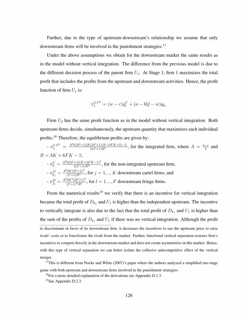
Further, due to the type of upstream-downstream’s relationship we assume that only

downstream firms will be involved in the punishment strategies.17

Under the above assumptions we obtain for the downstream market the same results as

in the model without vertical integration. The difference from the previous model is due to

the different decision process of the parent firm U1. At Stage 1, firm 1 maximizes the total

profit that includes the profits from the upstream and downstream activities. Hence, the profit

function of firm U1 is:

πV IK

1 = (w − c)qU1 + (a− bQ− w)qk1

Firm U2 has the same profit function as in the model without vertical integration. Both

upstream firms decide, simultaneously, the upstream quantity that maximizes each individual

profits.18 Therefore, the equilibrium profits are given by:

- πV IK1 = A2b(2F+1)[K(2F+1)(K+2FK+2)−1]2(F+1)B2 , for the integrated firm, where A = a−c

band

B = 3K + 6FK − 1;

- πU2 = A2b(2F+1)(K+2FK−1)2

2(F+1)B2 , for the non-integrated upstream firm;

- πDkj = A2bK(2F+1)2

(F+1)B2 , for j = 1, .., K downstream cartel firms; and

- πDfl = A2bK2(2F+1)2

(F+1)2B2 , for l = 1, .., F downstream fringe firms.

From the numerical results19 we verify that there is an incentive for vertical integration

because the total profit of Dk1 and U1 is higher than the independent upstream. The incentive

to vertically integrate is also due to the fact that the total profit of Dk1 and U1 is higher than

the sum of the profits of Dk1 and U1 if there was no vertical integration. Although the profit

to discriminate in favor of its downstream firm, it decreases the incentives to use the upstream price to raise

rivals’ costs or to foreclosure the rivals from the market. Further, functional vertical separation restores firm’s

incentives to compete fiercely in the downstream market and does not create asymmetries in this market. Hence,

with this type of vertical separation we can better isolate the collusive anticompetitive effect of the vertical

merger.17This is different from Nocke and White (2007)’s paper where the authors analyzed a simplified one-stage

game with both upstream and downstream firms involved in the punishment strategies.18For a more detailed explanation of the derivations see Appendix D.1.3.19See Appendix D.2.3.

128

of the independent upstream firm is lower than in the case without vertical integration, the

profits for the remaining downstream firms (cartel and fringe) are now higher. Also, when

there is vertical integration with a cartel firm, both wholesale and retail prices decrease and

the total quantity increase. Then, we conclude that the vertical merger with a cartel firm

decreases the double marginalization problem.

To verify that the cartel is statically stable we analyze both internal and external stability

conditions (D’Aspremont et al., 1983) and the conclusions are summarized by Proposition

5.3.

Proposition 5.3. When U1 and Dk1 are vertically integrated, downstream collusion is stati-


◦ Internal Stability Condition:20

K(2F+1)2

(F+1)B2 ≥ (2F+3)2(K−1)2

(F+2)2(6F−9K−6FK+10)2

◦ External Stability Condition:

(K+1)(2F−1)2

F [3(K+1)(2F−1)−1]2≤ K2(2F+1)2

(F+1)2B2

Using the results from the numerical simulation21 we conclude that for this model, collu-

sion is sustainable if and only if there are F +2 or F +3 cartel firms and ifK > 3. This is the

same result as in the model without vertical integration, however, in this case, there is a lower

bound for the number of cartel firms. If the number of firms in the cartel is small, for instance

K = 3, their profits attract fringe firms. Consequently, fringe firms find it desirable to join

the cartel, making the cartel statically unstable. However, with more firms in the cartel, the

individual profit obtained by a fringe firm when it stays out of the cartel is higher than the

profit that it would get if it joins the cartel, which ensures the external static stability. Hence,20Relatively to the ISC, here we have two situations: both downstream integrated and non-integrated cartel

firms can deviate to the fringe if their profits is not as great as they would have if they join the fringe. However,

due to the type of vertical relationship in this model, the vertical merger does not lead to foreclosure nor create

asymmetries in downstream market. Hence, both integrated and non-integrated cartel firms have the same profit

and therefore we only have one ISC.21See Appendix D.2.1.

129

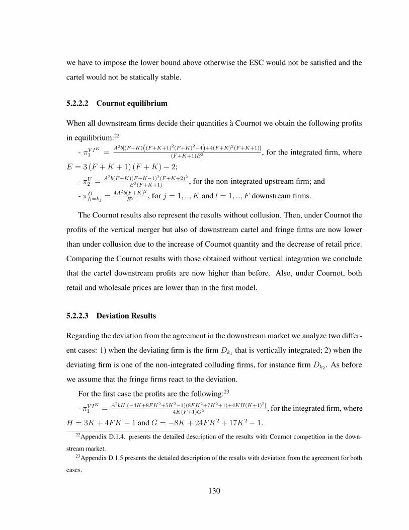
we have to impose the lower bound above otherwise the ESC would not be satisfied and the

cartel would not be statically stable.

5.2.2.2 Cournot equilibrium

When all downstream firms decide their quantities a Cournot we obtain the following profits

in equilibrium:22

- πV IK1 =A2b[(F+K)((F+K+1)2(F+K)2−4)+4(F+K)2(F+K+1)]

(F+K+1)E2 , for the integrated firm, where

E = 3 (F +K + 1) (F +K)− 2;

- πU2 = A2b(F+K)(F+K−1)2(F+K+2)2

E2(F+K+1), for the non-integrated upstream firm; and

- πDfl=kj = 4A2b(F+K)2

E2 , for j = 1, .., K and l = 1, .., F downstream firms.

The Cournot results also represent the results without collusion. Then, under Cournot the

profits of the vertical merger but also of downstream cartel and fringe firms are now lower

than under collusion due to the increase of Cournot quantity and the decrease of retail price.

Comparing the Cournot results with those obtained without vertical integration we conclude

that the cartel downstream profits are now higher than before. Also, under Cournot, both

retail and wholesale prices are lower than in the first model.


Regarding the deviation from the agreement in the downstream market we analyze two differ-

ent cases: 1) when the deviating firm is the firm Dk1 that is vertically integrated; 2) when the

deviating firm is one of the non-integrated colluding firms, for instance firm Dk2 . As before

we assume that the fringe firms react to the deviation.

For the first case the profits are the following:23

- πV IK1 = A2bH[(−4K+8FK2+5K2−1)(8FK2+7K2+1)+4KH(K+1)2]4K(F+1)G2 , for the integrated firm, where

H = 3K + 4FK − 1 and G = −8K + 24FK2 + 17K2 − 1.

22Appendix D.1.4. presents the detailed description of the results with Cournot competition in the down-

stream market.23Appendix D.1.5 presents the detailed description of the results with deviation from the agreement for both

cases.

130

- πU2 = A2bH(−4K+8FK2+5K2−1)2

4K(F+1)G2 , for the non-integrated upstream firm;

- πdk1= A2b(K+1)2H2

(F+1)G2 , for the deviation downstream cartel firm;

- πDkj = 2A2b(K+1)H2

(F+1)G2 , for the j = 2, .., K downstream cartel firms; and

- πDfl = A2b(K+1)2H2

(F+1)2G2 , for the l = 1, .., F downstream fringe firms.

By deviating from the collusive agreement, the integrated cartel downstream firm earns

higher profit than if it was in collusion, therefore it has incentives to deviate from the agree-

ment. Also, the total profit of the vertical integrated firm and the profit of the independent

upstream firm are higher than under collusion or without vertical integration. The profits of

the independent cartel firms and of fringe firms are lower than if they were in collusion.

Thereafter we present the constraint on the discount factor that ensures the dynamic sta-

bility of collusion. When U1 and Dk1 are vertically integrated, downstream collusion is dy-

namically stable if and only if:

δ ≥ E2[(K+1)2H2B2−K(2F+1)2G2]B2[(K+1)2H2E2−4(F+K)2(F+1)G2]

≡ δDk1

Under the second case Dk2 deviates from the collusive agreement, assuming that Dkj ,

with j = 1, .., K \ {2} produce the collusive quantities. The profits are the following:

- πV IF1 = A2b2K(K+1)H2+H(−2K+4FK2+3K2−1)(4FK2+3K2+1)

4K(F+1)I2 for the integrated firm, whereI =

−4K + 12FK2 + 9K2 − 1;

- πU2 = A2bH(−2K+4FK2+3K2−1)2

4K(F+1)I2 , for the non-integrated upstream firm;

- πdk2= A2bH2(K+1)2

4(F+1)I2 , for the deviation downstream cartel firm;

- πDkj = A2b(K+1)H2

2(F+1)I2 , for the j = 1, .., K \ {2} downstream cartel firms; and

- πDfl = Ab2H2(K+1)2

4(F+1)2I2 , for l = 1, .., F downstream fringe firms.

By deviating from the collusive agreement, the non-integrated cartel downstream firm

obtains higher profit. However, also the vertical integrated firm’s profit and the independent

upstream firm’s profits are higher. The remaining cartel firms’ profits and the fringe firms’

profits are lower.

131

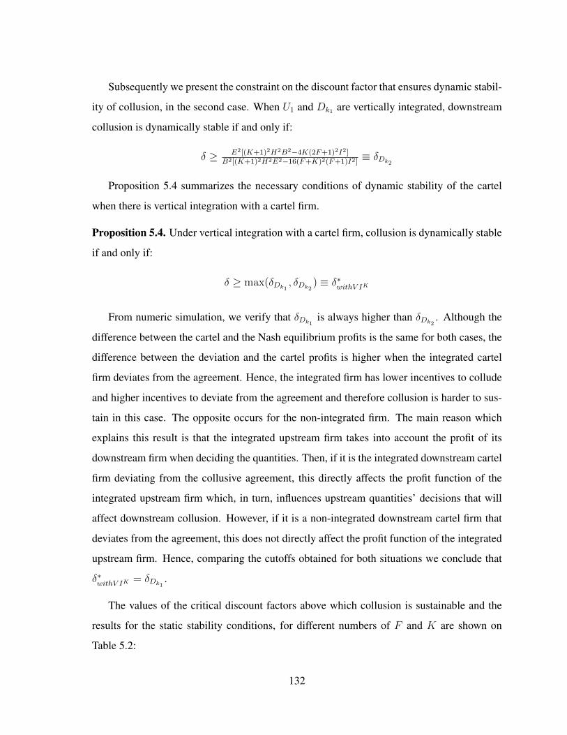
Subsequently we present the constraint on the discount factor that ensures dynamic stabil-

ity of collusion, in the second case. When U1 and Dk1 are vertically integrated, downstream

collusion is dynamically stable if and only if:

δ ≥ E2[(K+1)2H2B2−4K(2F+1)2I2]B2[(K+1)2H2E2−16(F+K)2(F+1)I2]

≡ δDk2

Proposition 5.4 summarizes the necessary conditions of dynamic stability of the cartel

when there is vertical integration with a cartel firm.

Proposition 5.4. Under vertical integration with a cartel firm, collusion is dynamically stable

if and only if:

δ ≥ max(δDk1, δDk2

) ≡ δ∗withV IK

From numeric simulation, we verify that δDk1is always higher than δDk2

. Although the

difference between the cartel and the Nash equilibrium profits is the same for both cases, the

difference between the deviation and the cartel profits is higher when the integrated cartel

firm deviates from the agreement. Hence, the integrated firm has lower incentives to collude

and higher incentives to deviate from the agreement and therefore collusion is harder to sus-

tain in this case. The opposite occurs for the non-integrated firm. The main reason which

explains this result is that the integrated upstream firm takes into account the profit of its

downstream firm when deciding the quantities. Then, if it is the integrated downstream cartel

firm deviating from the collusive agreement, this directly affects the profit function of the

integrated upstream firm which, in turn, influences upstream quantities’ decisions that will

affect downstream collusion. However, if it is a non-integrated downstream cartel firm that

deviates from the agreement, this does not directly affect the profit function of the integrated

upstream firm. Hence, comparing the cutoffs obtained for both situations we conclude that

δ∗withV IK = δDk1.

The values of the critical discount factors above which collusion is sustainable and the

results for the static stability conditions, for different numbers of F and K are shown on

Table 5.2:

132


K F δ∗withV IK

K F δ∗withV IK

3 1 0.882065∗ 8 6 0.997111

4 1 0.831454 9 6 0.991340

4 2 0.963883 9 7 0.998063

5 2 0.927391 10 7 0.993976

5 3 0.984628 10 8 0.998638

6 3 0.963152 11 8 0.995644

6 4 0.992100 11 9 0.999007

7 4 0.978966 12 9 0.996750

7 5 0.995419 12 10 0.999253

8 5 0.986926 ... ... ...∗For this value the ESC is not satisfied.

Analyzing Table 5.2 we conclude that, in order for collusion to be sustainable both stat-

ically and dynamically, we have to impose a lower bound for the number of cartel firms

(K > 3). As we can see, for K = 3 and F = 1 the external stability condition (ESC) is

not satisfied and therefore we do not have static stability. Once again, collusion is easier to

sustain the higher the number of cartel firms is and the lower the number of fringe firms is.

Comparing the results obtained by Proposition 5.4 with those obtained with Proposition

5.2 (see Table 5.1) we conclude that, for some level of market concentration, the vertical

merger with a cartel firm promotes collusion. However, due to the merger, collusion is less

easily sustained when the concentration in the market is low enough.

133

5.2.3 The Model of Vertical Integration with a fringe firm

Here we assume that there is vertical integration between one downstream fringe firm (Df1 ,

for instance) and one upstream firm (U1, for instance).


Again, we assume that although firmDf1 is vertically integrated with firmU1, it has autonomy

from the parent firm regarding the quantity decision.

The profit function of firm U1 is:

πV IF

1 = (w − c)qU1 + (a− bQK − bQF − w)qf1

Firm U2 has the same profit function as in the model without vertical integration. Both

upstream firms decide, simultaneously, the upstream quantity that maximizes each individual

profits.24 Therefore, the equilibrium profits are given by:

- πV IF1 = A2b2(F+1)(2F+1)2+F (2F+1)(2F+3)(3F+2F 2+2)

2(F+1)J2 , for the integrated firm, where J =

9F + 6F 2 + 2;

- πU2 = a2bF 2(2F+1)(2F+3)2

2(F+1)J2 , for the non-integrated upstream firm;

- πDkj = A2b(F+1)(2F+1)2

KJ2 , for j = 1, .., K downstream cartel firms; and

- πDfl = A2b(2F+1)2

J2 , for l = 1, .., F downstream fringe firms.

Looking at the numerical results25 we conclude that the profit of the vertically integrated

firm is always higher than the profit of the independent upstream firm U2. Once again, there

is an incentive for firms to vertically integrate because the total profit of the vertically inte-

grated firm is higher than the sum of the profits of Df1 and U1 without vertical integration.

The profits of the fringe and cartel firms are higher than in the case without vertical integra-

tion. That is, when there is vertical integration with a fringe firm, cartel firms have higher

incentives to collude and as we can see from the simulation, their profits are higher than

24For a more detailed explanation of the derivations see Appendix D.1.6.25See Appendix D.2.4.

134

the Cournot case or than the case where there is no vertical integration. Also, the vertical

merger with fringe firm reduces both wholesale and retail prices and increases the total quan-

tity in the market. Hence, as in the previous model, the vertical merger reduces the double

marginalization problem.

Once again to verify that the cartel is statically stable we have to ensure both internal and

external stability conditions:

◦ Internal Stability Condition:

K ≤ (2F+1)2(F+1)(21F+6F 2+17)2

(2F+3)2J2

◦ External Stability Condition:

K ≥ F (2F−1)2J2

(−3F+6F 2−1)2(2F+1)2 − 1

Proposition 5.5. When U1 and Df1 are vertically integrated, downstream collusion is stati-


F (2F+1)2J2

(−3F+6F 2−1)2(2F+1)2 − 1 ≤ K ≤ (2F+1)2(F+1)(21F+6F 2+17)2

(2F+3)2J2

Using the results from the numerical simulation26 we conclude that collusion is sustain-

able if and only if there are F +2 or F +3 cartel firms and if F > 1. This is the same result as

in the model without vertical integration, however here there is a lower bound for the number

of fringe firms. If there is only one fringe firm (F = 1), this firm finds it desirable to join

the cartel, making the cartel statically unstable. However, with more firms in the fringe, the

individual profit obtained by a fringe firm when it stays out of the cartel is higher than the

profit that it would get if it joins the cartel. Hence, fringe firms have no incentives to join the

cartel and therefore the external static stability condition is ensured. Then, in order to satisfy

the ESC and ensure the static stability of the cartel we impose the lower bound above.

26See Appendix D.2.1.

135

5.2.3.2 Cournot equilibrium

The Cournot results are the same as in the previous model because at the downstream market

all firms have the same behavior.


Considering that, for instance firm Dk1 deviates from the collusive agreement and, as before,

the fringe firms react to the deviation, the profits are the following:27

- πV IF1 = A2b4K(F+1)(K+1)2H2+(K+2FK−1)(5K+4FK+1)(14FK2+8F 2K2−2FK+7K2+1)H

4KL2(F+1), for

the integrated firm, with L = −8K + 42FK2 + 24F 2K2 − 6FK + 17K2 − 1;

- πU2 = A2bH(K+2FK−1)2(5K+4FK+1)2

4KL2(F+1), for the non-integrated upstream firm;

- πdk1= A2b (F+1)(K+1)2H2

L2 , for the deviation downstream cartel firm;

- πDkj = 2A2b (F+1)(K+1)H2

L2 , for the j = 2, .., K downstream cartel firms; and

- πDfl = A2bH2(K+1)2

L2 , for the l = 1, .., F downstream fringe firms.

By deviating from the collusive agreement, the cartel firm earns higher profit. However,

if the firm does not deviate it will earn lower profit than if there were no vertical integration.

Then the incentives to deviate from the collusive agreement are lower. The constraint de-

scribed by Proposition 5.6 ensure that collusion is dynamically stable.

Proposition 5.6. When U1 and Df1 are vertically integrated, downstream collusion is dy-

namically stable if and only if:

δ ≥ E2[(F+1)(K+1)2H2KJ2−(F+1)(2F+1)2L2]KJ2[(F+1)(K+1)2H2E2−4(F+K)2L2]

≡ δ∗withV IF

Table 5.3 shows the values of the critical discount factors above which collusion is sus-

tainable and the results of the static stability conditions, for different number of F and K

firms:27Appendix D.1.7. presents the detailed description of the results with deviation.

136


K F δ∗withV IF K F δ∗withV IF

3 1 0.744721∗ 8 6 0.996443

4 1 0.724597∗ 9 6 0.990245

4 2 0.940123 9 7 0.997678

5 2 0.901072 10 7 0.993323

5 3 0.977686 10 8 0.998401

6 3 0.953961 11 8 0.995231

6 4 0.989391 11 9 0.998853

7 4 0.974993 12 9 0.996476

7 5 0.994154 12 10 0.999149

8 5 0.984944 ... ... ...∗For these values the ESC is not satisfied.

From the results in Table 5.3 we conclude the cartel is not statically stable for F = 1

because the external stability condition is not satisfied. Then, only when there are F+2 or F+

3 and when F > 1 collusion is stable. Again, collusion is more difficult to sustain the lower

the number of cartel firms is and the higher the number of fringe firms is. Further, comparing

the results obtained with Proposition 5.6 with those obtained in Proposition 5.2 (see Table 5.1)

it is possible to conclude that vertical merger with a fringe firm always promotes collusion.

5.3 Welfare analysis

In this section we discuss the social welfare implications of the three models.

When there is vertical integration we can have two main effects. On one hand, we have

the collusive effects, that is, vertical integration increases the incentives for downstream firms

to collude. With high incentives to collude, downstream firms will increase the retail price

(P ) and decrease the total quantity (Q), which harms the social welfare. On the other hand,

137

vertical integration has efficiency effects: with the vertical merger the total retail quantity

increases and the retail price decreases, when comparing with the situation without the ver-

tical merger (model 1).28 Also, the vertical merger increases upstream competition which

decreases the wholesale price (w). Further, we find that the vertical integration (models 2 and

3) reduces the problem of double marginalization, but it does not solve it because upstream

firms are still setting the input price above their marginal cost. The reduction of the double

marginalization problem could also be obtained with other vertical restraints (for instance,

non-linear prices, royalties, resale price maintenance, among others) or even without collu-

sion (for instance, under Cournot). We find that the reduction of the double marginalization

problem triggered by the vertical merger is higher in the presence of collusion than without

it. Also, in this paper we assume that there are only two upstream firms. We believe that

the double marginalization problem could be totally eliminated if we increase the number of

upstream firms.

We conclude that the positive effects more than compensate the negative effects which

explains why there is an improvement in welfare when we move from model 1 to models 2

and 3.

Table 5.4 displays the differences of social welfare (SW) between models 1 and 2 and

between models 1 and 3, decomposing it into the variation of consumer surplus (CS) and

producer surplus (PS).

28In the comparison of prices and quantities for the three models, we assume that a = 1, b = 1 and c = 0.5.

We verify that changes in the values of the parameters a, b and c do not modify the discussion of the results

among the three models nor the variation of social welfare. More details on the calculations can be provided

upon request to the authors.

138

Table 5.4: Welfare analysis

Model 1 vs Model 2 Model 1 vs Model 3

K F 4 PS % 4 CS % 4 SW % 4 PS % 4CS % 4 SW %

3 1 - - - - - -

4 1 -0.08% 5.80% 1.88% - - -

4 2 -0.46% 3.42% 1.03% -0.63% 4.60% 1.38%

5 2 -0.36% 2.72% 0.82% -0.63% 4.60% 1.38%

5 3 -0.40% 1.93% 0.56% -0.50% 2.42% 0.70%

6 3 -0.33% 1.61% 0.47% -0.50% 2.42% 0.70%

6 4 -0.32% 1.25% 0.35% -0.38% 1.50% 0.42%

7 4 -0.27% 1.07% 0.30% -0.38% 1.50% 0.42%

7 5 -0.25% 0.87% 0.24% -0.29% 1.02% 0.28%

8 5 -0.22% 0.76% 0.21% -0.29% 1.02% 0.28%

8 6 -0.20% 0.64% 0.18% -0.23% 0.74% 0.20%

9 6 -0.18% 0.57% 0.16% -0.23% 0.74% 0.20%

9 7 -0.17% 0.50% 0.13% -0.19% 0.56% 0.15%

10 7 -0.15% 0.45% 0.12% -0.19% 0.56% 0.15%

10 8 -0.14% 0.39% 0.11% -0.15% 0.44% 0.12%

11 8 -0.13% 0.36% 0.10% -0.15% 0.44% 0.12%

11 9 -0.12% 0.32% 0.09% -0.13% 0.35% 0.09%

12 9 -0.11% 0.29% 0.08% -0.13% 0.35% 0.09%

12 10 -0.10% 0.27% 0.07% -0.11% 0.29% 0.08%

As we can observe from Table 5.4, under incomplete collusion, the social welfare in-

creases when we move from an industry with no vertical integration to an industry where

there is vertical integration either with a cartel or a fringe downstream firm. This is also true

when we compare the results obtained under Cournot. With vertical integration, consumers

see their welfare improving because the total quantity in the market increases. Also, firms

139

have lower profits due to the reduction of both retail and wholesale prices. The increase in

the consumer surplus is higher than the decrease in the producer surplus, hence the net ef-

fect is that vertical integration increases social welfare. These efficiency effects are similar

in both models 2 and 3, however the vertical merger with a fringe firm increases more the

total quantity in the market than the vertical merger with a cartel firm. This explains why the

increase of the social welfare is higher in model 3 than in model 2.

5.4 Discussion of Results

In order to verify if vertical integration promotes collusion, we compare the results of the

dynamic and static stability conditions for the three models.29

From the numerical results we conclude that, for the first model, the participation condi-

tions are verified if the number of cartel firms are F +2 or F +3, that is the cartel should have

respectively, 50% − 75% or 50% − 80% firms in the industry. However, for models 2 and 3

we have to introduce additional assumptions (K > 3 and F > 1, respectively) otherwise, the

external stability conditions (ESC) are not satisfied and therefore the cartel would become

statically unstable.

As mentioned in section 5.3, we identify two effects of the vertical merger: the effi-

ciency effect and the collusive effect. Under trigger strategies, the non-cooperative collusion

is stable because the difference between deviation and collusive payoffs is large enough to

outweigh, in present discounted value, the difference between collusive and NE payoffs. For

a downstream cartel firm, vertical integration increases the difference between collusive and

NE payoffs so tends to increase cartel stability. Therefore, vertical integration has a collusive

effect in the downstream market.30 However, this collusive effect is distinct when we analyse

a merger with a fringe firm or a merger with a cartel firm.

29See Appendix D.2.1.30The collusive effect obtained in this paper is different from Chen (2001) ’s because we have different

model’s specifications. Chen (2001) argues that the vertical merger softens price competition in the final

market and changes rival’s incentive in selecting input suppliers.

140

Figure 5.1: Model’s critical discount values for K=F+2

Figure 5.2: Model’s critical discount values for K=F+3

141

After analyzing the critical discount values (Figures 5.1 and 5.2), we conclude that verti-

cal integration always promotes collusion when the upstream firm merges with a downstream

fringe firm. This is justified because vertical integration with a fringe firm reinforces the

incentives for the cartel firms not to deviate from the collusive agreement. As the vertical

integrated firm is now in a privileged position, cartel firms take this as a threat and therefore

react defensively against this competitive firm. Furthermore, there is an incentive for firms

to vertically integrate because the profit of the vertical integrated firm is higher than the sum

of profits of a Df and an U firms, without vertical integration. Also, although the vertical

merger increases the difference between the collusive and NE payoffs, it also decreases the

difference between deviation and collusive payoffs. Since the second difference is higher

than the first, the vertical merger with a fringe firm decreases the critical discount factor (δ∗)

and therefore increases the cartel stability, for any level of downstream market concentration.

Differently, it is possible to find situations where vertical integration with a cartel firm

hinders collusion. This depends on the number of firms in the downstream market. Although

there is an incentive to vertically integrate due to the possibility of getting higher profits, this

could make collusion more difficult to sustain. For example, for K = 4 and F = 2, vertical

integration either with a fringe or a cartel firm promotes collusion. Also, for this case, vertical

integration with a fringe firm incentives more the collusion than vertical integration with a

cartel firm. But for K = 8 and F = 5 vertical integration increases cartel sustainability

only when it is with a fringe firm. One reason that explains why collusion is more difficult

to sustain when there is vertical integration with a cartel firm, is the low level of market

concentration. With a high number of firms in the market, the vertically integrated firm

continues to have higher profit than its rivals, however cartel individual profits will be lower

because they have to share the cartel total profit with a high number of firms and therefore they

will earn more from deviating. Also, although the vertical merger increases the difference

between the collusive and the NE payoffs, it also increases the difference between deviation

and collusive payoffs. Thus, since the second difference is higher than the first, the vertical

merger with a cartel firm increases the critical discount factor (δ∗) and makes collusion harder

to sustain.

142

Moreover, with the merger the collusive and the deviation profit of each cartel firm in-

crease in both models: when the merger is with a fringe firm, cartel firms have higher collu-

sive profits than when the merger is with cartel firms. Also, when the merger is with a fringe

firm, cartel firms have less incentives to deviate from the collusive agreement than when the

merger is with a cartel firm, because the cartel deviation profit in the third model is lower

than in the second model. This explains why the vertical merger with a fringe firm increases

more the incentives to collude than the merger with a cartel firm.

Furthermore, in both cases, we identify the efficiency effects of the vertical merger. The

vertical merger with a cartel or a fringe downstream firm makes the upstream market asym-

metric and this asymmetry is higher in model 3 than in model 2. Hence, with the verti-

cal merger the upstream competition increases and therefore the final result is that the total

wholesale quantity increases. This increase in the total quantity is smaller the larger is the

number of downstream firms. Also, the increase of the wholesale quantity is higher in model

3 than in model 2. With higher wholesale quantity, both wholesale and retail prices decrease,

which in turn, increase the quantity produced by the downstream firms and affects the stability

of collusion. Thus, the increase in upstream competition also affects downstream collusion.

Then, similar to Chen (2001)’s model, the vertical merger generates efficiency gains because

the merged firm improves the production of its inputs and also intensifies price competition in

the final market. Also, the vertical merger is efficiency increasing because, as we mentioned

in the previous section, it reduces the double marginalization problem and this reduction is

higher when there is collusion than if there was no collusion.

Summarizing, the vertical merger with a fringe firm always promotes downstream col-

lusion while if the merger is with a cartel firm we can have the two situations for different

levels of market concentration. For low level of market concentration, the vertical merger

with a cartel firm increases the difference between the collusive and NE profits. This increase

however decreases as the number of downstream firms increase and consequently vertical

integration with a cartel firm hinders collusion.

We compare models 1 and 2 to evaluate the difference between our results and those ob-

tained if there was full collusion (F = 0). We conclude that when an incomplete cartel faces

143

outsider competition it has a limited ability to charge a price above competition levels. Hence,

when the cartel is not all-inclusive the collusive prices are lower than under complete collu-

sion and therefore, incomplete collusion is harder to sustain than complete collusion. Also,

this explains why when the cartel is incomplete, the sustainability of collusion decreases, the

higher the number of fringe firms is. Moreover, we conclude that, under full collusion, a

vertical merger with a cartel firm always promotes collusion for low level of market concen-

tration (K ≤ 5). However, with a high number of cartel firms, the vertical merger with a

cartel firm also hinders collusion. This results are similar to those obtained with incomplete

collusion.

5.5 Concluding Remarks

This paper explores the effect of vertical integration on the incentives to collude, when there

is incomplete collusion in the downstream market. A central result of the paper is that in

general by acquiring a downstream firm (a cartel or a fringe firm), the vertically integrated

firm promotes collusion at downstream level. The vertical merger increases the cartel firms’

incentives to collude and decreases the deviation incentives from the collusive agreement.

However, for low downstream market concentration, the opposite result is found when

the vertical merger is with a cartel downstream firm. The larger the number of cartel firms is

the lower the profit that each cartel firm earns and therefore the higher the incentive to disrupt

the collusive agreement is. Hence, vertical integration with a cartel firm hinders downstream

collusion for high number of cartel firms in downstream market. The results we found are

very important to understand the type of strategies that firms follow in markets where there

is incomplete collusion and vertical integration. Further, the combination of these two types

of strategies does not have the same effects in markets with different level of concentration.

In spite of collusion, we verify that vertical integration increases social welfare due to the

partial elimination of double marginalization. These results could be important for antitrust

authorities that are concerned with the effects of such mergers on downstream collusion.

The framework and the assumptions we have assumed are of a particular kind. Further

144

research on the analysis of the relationship between vertical merger and incomplete collusion

should consider what happens if there is vertical integration with more than one downstream

firm. Also, it would be interesting to study the case where the downstream firm also takes into

account the profits of the upstream firm, relaxing the assumption that it has an independent

behavior from the upstream firm. We think that these are very important and useful subjects

for further research.

145

Appendix

Appendix D.1. Equilibrium Profits

Appendix D.1.1. Cournot profits for non-integrated equilibrium - Model 1

Under this case all downstream firms decide individually their quantity. Knowing that

the firms are symmetric, the quantity produced by each downstream firm is given by: qkj =

qfl = a−wb(F+K+1)

, with j = 1, .., K and l = 1, ..., F . Therefore, the inverse demand function

to upstream firms is w = a− b(F+K+1)QF+K

. At stage 1, the upstream firms decide the quantity,

maximizing their profits functions: πUi = (w − c)qUi = (a(F+K)−b(F+K+1)(qUi +qU2 )

F+K− c)qUi ,

with i = 1, 2. The equilibrium results are:

qUi = A(F+K)3(F+K+1)

, with A = a−cb

qDkj = qDfl = 2A3(F+K+1)

.

P = a(3+F+K)+2c(F+K)3(F+K+1)

w = a+2c3

πUi = A2b(F+K)9(F+K+1)

πDkj = πDfl = 4A2b9(F+K+1)2 .

Appendix D.1.2. Deviation profits for non-integrated firms - Model 1

FirmDk1 deviates from the collusive agreement knowing that firmsDkj , with j = 2, .., K,

produce the collusive quantities and fringe firms Dfl , with l = 1, .., F , react to the deviation.

Then residual demand for the deviating firm is given by: P = a− bqdk1− (K − 1)a−w

2K−

F a−w−bQK(F+1)

and the deviation quantity is qdeviationk1= (a−w)(K+1)

4bK.

At stage 1 the upstream firms decide the quantity, knowing that w = a− 4b(F+1)QH

, where

H = 3K + 4FK − 1. Then the upstream firms will produce ,in equilibrium, qUi = AH12K(F+1)

,

with i = 1, 2. The equilibrium prices are given by w = a+2c3

and P = a(3K+2FK+1)+cH6K(F+1)

and the downstream quantities are qdeviationk1= A(K+1)

6K, qkj = A

3K, with j = 2, .., K and

qfl = A(K+1)6K(F+1)

, with l = 1, .., F . The equilibrium profits are:

πUi = A2bH36K(F+1)

πdeviationk1= A2b(K+1)2

36K2(F+1)

πDkj = A2b(K+1)18K2(F+1)

, with j = 2, .., K πDfl = A2b(K+1)2

36K2(F+1)2 , with l = 1, .., F .

146

Appendix D.1.3. Collusion profits under Vertical Integration with a Cartel down-

stream firm - Model 2

At Stage 1, upstream firm 1, vertically integrated, maximizes the total profit that includes

the profits from the upstream and downstream activities. Upstream firm 2 maximizes its own

profit. Hence, the profit functions of firms U1 and U2 are:

πV IK

1 = (w − c)qU1 + (a− bQ− w)qk1

πU2 = (w − c)qU2

where w = a(2F+1)−2bQ(F+1)2F+1

, qk1 = a−w2bK

and Q = qU1 + qU2 . Then the upstream

firms will produce, in equilibrium, qU1 = A(2F+1)(K(2F+1)+1)2B(F+1)

and qU2 = A(2F+1)(K(2F+1)−1)2B(F+1)

,

where A = a−cb and B = 3K + 6FK − 1. By substitution we obtain the equilibrium prices

w = a(K(2F+1)−1)+2Kc(2F+1)B

and P =a((F+1)B−K(2F+1)2)+K(2F+1)2c

B(F+1)and the equilibrium

quantities for the downstream cartel and fringe firms qk1 = A(2F+1)B

and qfl = AK(2F+1)B(F+1)

.

The equilibrium profits are:

πV IK

1 = A2b(2F+1)[K(2F+1)(K+2FK+2)−1]2(F+1)B2 πU2 = A2b(2F+1)(K+2FK−1)2

2(F+1)B2

πDkj = A2bK(2F+1)2

(F+1)B2 , for j = 2, .., K πDfl = A2bK2(2F+1)2

(F+1)2B2 , for l = 1, .., F.

Appendix D.1.4. Cournot profits under Vertical Integration with a Cartel or Fringe

downstream firm - Models 2 and 3

Assuming that the downstream integrated behaves as a subsidiary firm that decides its

quantity in an independent way from the parent upstream firm, the first stage the results are

the same as in the model without vertical integration. The profit functions for upstream firms

are:

πV IK

1 = (w − c)qU1 + (a− b(qU1 + qU2 )− w)qk1

πU2 = (w − c)qU2

which lead to the following results:

qU1 = A(F+K)[(F+K+1)(F+K)+2](F+K+1)E

, where E = 3(F +K + 1)(F +K)− 2)

147

qU2 = A(F+K)(F+K−1)(F+K+2)(F+K+1)E

w = a[(F+K+1)(F+K)−2]+2c(F+K)(F+K+1)E

P = a[(F+K)2+3(F+K)−2]+2c(F+K)2

E

qkj = qfk = 2A(F+K)E

, with j = 1, .., K and l = 1, .., F .

πU2 = A2b(F+K)(F+K−1)(F+K+2)[(F+K+1)(F+K)−2]E2(F+K+1)

πDkj = πDfl = 4A2b(F+K)2

E2 , with j = 1, .., K and l = 1, .., F .

πV I1 = A2b(F+K)[(F+K+1)2(F+K)2−4](F+K+1)E2 + 4A2b(F+K)2

E2

Appendix D.1.5. Deviation profits under Vertical Integration with a Cartel downstream

firm - Model 2

First Case: Dk1 , that is vertically integrated, deviates from the collusive agreement know-

ing that Dkj , for j = 2, .., K produce the collusive quantities and that fringe firms Dfl react

to the deviation.

The residual demand for firm Dk1 is: P = a− bqdeviationk1− (K − 1)ba−w

2bK− bF a−w−bQK

b(F+1)

and the quantity is qdeviationk1= (K+1)(a−w)

4bK. The upstream firms maximize their profits, given

by

πV I1 = (w − c)qU1 + (a− b(qU1 + qU2 )− w)qdeviationk1

πU2 = (w − c)qU2

knowing that w = a− 4bK(F+1)QH

.

Then the equilibrium quantities, prices and profits are given by:

qU1 = AH(8FK2+7K2+1)4K(F+1)G

, where G = −8K + 24FK2 + 17K2 − 1

qU2 = AH(−4K+8FK2+5K2−1)4K(F+1)G

w = a(8FK2+5K2−4K−1)+4cKHG

P = a(8F 2K2+17FK2+8K2−F−2K−2)+cH2

(F+1)G

qdeviationk1= AH(K+1)

Gqfl = AH(K+1)

G(F+1), with l = 1, .., F qkj = 2AH

G, with

j = 2, .., K

πU2 = A2b(−4K+8FK2+5K2−1)2H4KG2(F+1)

πdeviationk1= A2b(K+1)2H2

(F+1)G2

πDkj = 2A2b(K+1)H2

(F+1)G2 πDfl = A2b(K+1)2H2

(F+1)2G2

πV IK

1 = A2b(−4K+8FK2+5K2−1)(8FK2+7K2+1)H4KG2(F+1)

+A2b(K+1)2H2

(F+1)G2

148

Second Case: Dk2 deviates from the collusive agreement, knowing that Dkj , with j =

1, .., K \ {2} produce the collusive quantities and the fringe downstream firms react to that

deviation.

The residual demand for firm Dk2 is given by P = a − bqdeviationk2− (K − 1) ∗ a−w

2K−

bF a−w−bQK(F+1)b

and the deviation quantity is qdeviationk2= (a−w)(K+1)

4bK.

The upstream firms maximize their profits, knowing that w = a − 4K(F+1)QbH

. Then the

equilibrium quantities, prices and profits are given by:

qU1 = AH(4FK2+3K2+1)4K(F+1)I

, where I = −4K+12FK2+9K2−1 qU2 = A(−2K+4FK2+3K2−1)H4K(F+1)I

w = a(4FK2+3K2−2K−1)+2cKHI

P = a(8F 2K2+18FK2+9K2−2F−2K−3)+cH2

2(F+1)I

qdeviationk2= AH(K+1)

2Iqfl = AH(K+1)

2I(F+1)qkj = AH

I

πU2 = A2bH(−2K+4FK2+3K2−1)2

4KI2(F+1)

πdeviationk2= A2b(K+1)2H2

4(F+1)I2 πDkj = A2b(K+1)H2

2(F+1)I2 , with j = 1, .., K\{2}

πDfl = A2b(K+1)2H2

4(F+1)2I2 , with l = 1, .., F

πV IK

1 = A2b(K+1)H2

2(F+1)I2 + A2(−2K+4FK2+3K2−1)(4FK2+3K2+1)H4KI2(F+1)

Appendix D.1.6. Collusion profits under Vertical Integration with a Cartel downstream

firm - Model 3

At Stage 1, uptream firm 1, vertically integrated, maximizes the total profit that includes

the profits from the upstream and downstream activities. Upstream firm 2 maximizes its own

profit. Hence, the profit functions of firms U1 and U2 are:

πV IF

1 = (w − c)qU1 + (a− bQK − bQF − w)qf1

πU2 = (w − c)qU2

The equilibrium upstream quantities are given by: qU1 =A(2F+1)(3F+2F 2+2)

2(F+1)J, where J =

9F + 6F 2 + 2 and qU2 = AF (2F+3)(2F+1)2(F+1)J

. By substitution we obtain the equilibrium prices

w = 2c(2F 2+3F+1)+a(2F 2+3F )J

and P = a(2F 2+5F+1)+c(4F 2+4F+1)J

and the equilibrium quantities

for the downstream cartel and fringe firms qkj = A(F+1)(2F+1)KJ

and qfl = A(2F+1)J

. The

equilibrium profits are:

πV IF

1 = A2b2(F+1)(2F+1)2+F (2F+1)(2F+3)(3F+2F 2+2)

2(F+1)J2 πU2 = a2bF 2(2F+1)(2F+3)2

2(F+1)J2

149

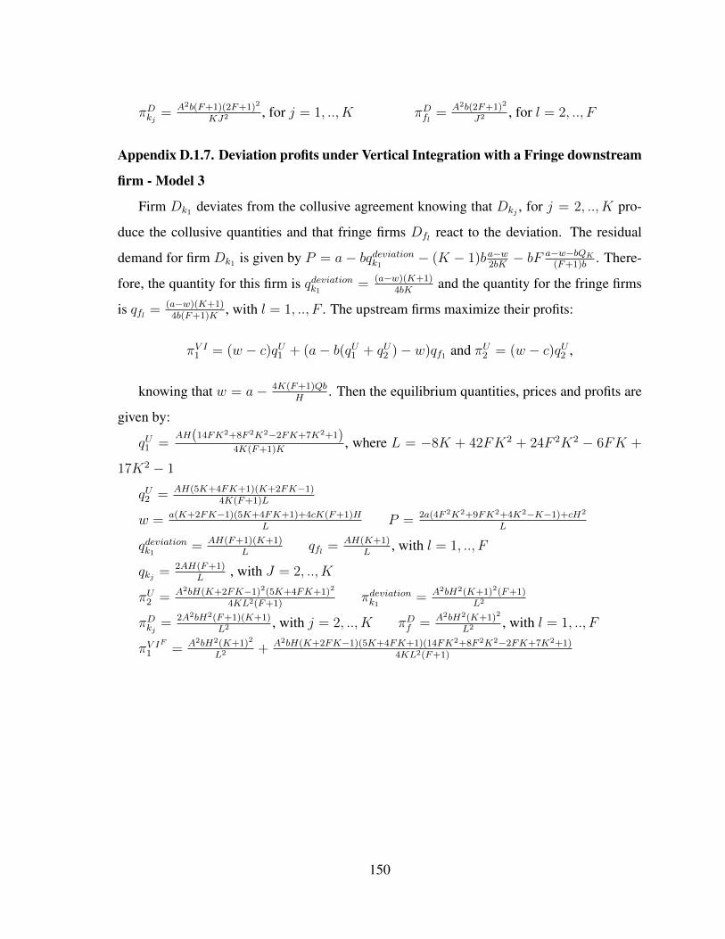
πDkj = A2b(F+1)(2F+1)2

KJ2 , for j = 1, .., K πDfl = A2b(2F+1)2

J2 , for l = 2, .., F

Appendix D.1.7. Deviation profits under Vertical Integration with a Fringe downstream

firm - Model 3

Firm Dk1 deviates from the collusive agreement knowing that Dkj , for j = 2, .., K pro-

duce the collusive quantities and that fringe firms Dfl react to the deviation. The residual

demand for firm Dk1 is given by P = a− bqdeviationk1− (K − 1)ba−w

2bK− bF a−w−bQK

(F+1)b. There-

fore, the quantity for this firm is qdeviationk1= (a−w)(K+1)

4bKand the quantity for the fringe firms

is qfl = (a−w)(K+1)4b(F+1)K

, with l = 1, .., F . The upstream firms maximize their profits:

πV I1 = (w − c)qU1 + (a− b(qU1 + qU2 )− w)qf1 and πU2 = (w − c)qU2 ,

knowing that w = a− 4K(F+1)QbH

. Then the equilibrium quantities, prices and profits are

given by:

qU1 =AH(14FK2+8F 2K2−2FK+7K2+1)

4K(F+1)K, where L = −8K + 42FK2 + 24F 2K2 − 6FK +

17K2 − 1

qU2 = AH(5K+4FK+1)(K+2FK−1)4K(F+1)L

w = a(K+2FK−1)(5K+4FK+1)+4cK(F+1)HL

P = 2a(4F 2K2+9FK2+4K2−K−1)+cH2

L

qdeviationk1= AH(F+1)(K+1)

Lqfl = AH(K+1)

L, with l = 1, .., F

qkj = 2AH(F+1)L

, with J = 2, .., K

πU2 = A2bH(K+2FK−1)2(5K+4FK+1)2

4KL2(F+1)πdeviationk1

= A2bH2(K+1)2(F+1)L2

πDkj = 2A2bH2(F+1)(K+1)L2 , with j = 2, .., K πDf = A2bH2(K+1)2

L2 , with l = 1, .., F

πV IF

1 = A2bH2(K+1)2

L2 + A2bH(K+2FK−1)(5K+4FK+1)(14FK2+8F 2K2−2FK+7K2+1)4KL2(F+1)

150

Appendix D.2. Numerical SimulationAppendix D.2.1. Results from Static and Dynamic Stability31

Static Stability Dynamic Stability

Model 1 Model 2 Model 3 Model 1 Model 2 Model 3

K F δ∗withoutV I δ∗Dk1δ∗Dk2

δ∗withV IF

3 1 ESC No ESC No ESC 0.892857 0.882065 0.860994 0.744721

ISC ISC ISC

4 1 ESC ESC No ESC 0.835052 0.831454 0.812044 0.724597

ISC ISC ISC

4 2 ESC ESC ESC 0.964989 0.963883 0.960915 0.940123

ISC ISC ISC

5 2 ESC ESC ESC 0.927536 0.927391 0.922718 0.901072

ISC ISC ISC

5 3 ESC ESC ESC 0.984802 0.984628 0.983868 0.977686

ISC ISC ISC

6 3 ESC ESC ESC 0.963020 0.963152 0.961592 0.953961

ISC ISC ISC

6 4 ESC ESC ESC 0.992129 0.992100 0.991830 0.989391

ISC ISC ISC

7 4 ESC ESC ESC 0.978852 0.978966 0.978320 0.974993

ISC ISC ISC

7 5 ESC ESC ESC 0.9954188 0.9954187 0.995301 0.994154

ISC ISC ISC

8 5 ESC ESC ESC 0.986848 0.986926 0.986615 0.984944

ISC ISC ISC

8 6 ESC ESC ESC 0.997106 0.997111 0.997052 0.996443

ISC ISC ISC

9 6 ESC ESC ESC 0.991288 0.991340 0.991174 0.990245

ISC ISC ISC

9 7 ESC ESC ESC 0.998057 0.998063 0.998030 0.997678

ISC ISC ISC

10 7 ESC ESC ESC 0.993940 0.993976 0.993879 0.993323

ISC ISC ISC

10 8 ESC ESC ESC 0.998634 0.998638 0.998619 0.998401

ISC ISC ISC

11 8 ESC ESC ESC 0.995619 0.995644 0.995584 0.995231

ISC ISC ISC

11 9 ESC ESC ESC 0.999003 0.999007 0.998994 0.998853

ISC ISC ISC

12 9 ESC ESC ESC 0.996732 0.996750 0.996711 0.996476

ISC ISC ISC

12 10 ESC ESC ESC 0.999251 0.999253 0.999245 0.999149

ISC ISC ISC

31Note that ESC - External Stability Condition and ISC - Internal Stability Condition.

151

Appendix D.2.2. Results for Model 132

a) Collusive Results

K F U qt K qt F qt U profit K profit F profit

3 1 0.25000 0.11111 0.16667 0.08333 0.01852 0.02778

4 1 0.25000 0.08333 0.16667 0.08333 0.01389 0.02778

4 2 0.27778 0.08333 0.11111 0.09259 0.00926 0.01235

5 2 0.27778 0.06667 0.11111 0.09259 0.00741 0.01235

5 3 0.29167 0.06667 0.08333 0.09722 0.00556 0.00694

6 3 0.29167 0.05556 0.08333 0.09722 0.00463 0.00694

6 4 0.30000 0.05556 0.06667 0.10000 0.00370 0.00444

7 4 0.30000 0.04762 0.06667 0.10000 0.00317 0.00444

7 5 0.30556 0.04762 0.05556 0.10185 0.00265 0.00309

8 5 0.30556 0.04167 0.05556 0.10185 0.00231 0.00309

8 6 0.30952 0.04167 0.04762 0.10317 0.00198 0.00227

9 6 0.30952 0.03704 0.04762 0.10317 0.00176 0.00227

9 7 0.31250 0.03704 0.04167 0.10417 0.00154 0.00174

10 7 0.31250 0.03333 0.04167 0.10417 0.00139 0.00174

10 8 0.31481 0.03333 0.03704 0.10494 0.00123 0.00137

11 8 0.31481 0.03030 0.03704 0.10494 0.00112 0.00137

11 9 0.31667 0.03030 0.03333 0.10556 0.00101 0.00111

12 9 0.31667 0.02778 0.03333 0.10556 0.00093 0.00111

12 10 0.31818 0.02778 0.03030 0.10606 0.00084 0.00092

b) Cournot Results

K F U qt K qt=F qt U profit K=F profit

3 1 0.26667 0.13333 0.08889 0.01778

4 1 0.27778 0.11111 0.09259 0.01235

4 2 0.28571 0.09524 0.09524 0.00907

5 2 0.29167 0.08333 0.09722 0.00694

5 3 0.29630 0.07407 0.09877 0.00549

6 3 0.30000 0.06667 0.10000 0.00444

6 4 0.30303 0.06061 0.10101 0.00367

7 4 0.30556 0.05556 0.10185 0.00309

7 5 0.30769 0.05128 0.10256 0.00263

8 5 0.30952 0.04762 0.10317 0.00227

8 6 0.31111 0.04444 0.10370 0.00198

9 6 0.31250 0.04167 0.10417 0.00174

9 7 0.31373 0.03922 0.10458 0.00154

10 7 0.31481 0.03704 0.10494 0.00137

10 8 0.31579 0.03509 0.10526 0.00123

11 8 0.31667 0.03333 0.10556 0.00111

11 9 0.31746 0.03175 0.10582 0.00101

12 9 0.31818 0.03030 0.10606 0.00092

12 10 0.31884 0.02899 0.10628 0.00084

32Note that the quantities are multiplied by A = a−cb and the profits by A2b.

152

c) Deviating Results

K F U qt K1 qt dev K qt F qt U profit K profit K dev profit F profit

3 1 0.27778 0.22222 0.11111 0.11111 0.09259 0.00617 0.02469 0.01235

4 1 0.28125 0.20833 0.08333 0.10417 0.09375 0.00347 0.02170 0.01085

4 2 0.29861 0.20833 0.08333 0.06944 0.09954 0.00347 0.01447 0.00482

5 2 0.30000 0.20000 0.06667 0.06667 0.10000 0.00222 0.01333 0.00444

5 3 0.30833 0.20000 0.06667 0.05000 0.10278 0.00222 0.01000 0.00250

6 3 0.30903 0.19444 0.05556 0.04861 0.10301 0.00154 0.00945 0.00236

6 4 0.31389 0.19444 0.05556 0.03889 0.10463 0.00154 0.00756 0.00151

7 4 0.31429 0.19048 0.04762 0.03810 0.10476 0.00113 0.00726 0.00145

7 5 0.31746 0.19048 0.04762 0.03175 0.10582 0.00113 0.00605 0.00101

8 5 0.31771 0.18750 0.04167 0.03125 0.10590 0.00087 0.00586 0.00098

8 6 0.31994 0.18750 0.04167 0.02679 0.10665 0.00087 0.00502 0.00072

9 6 0.32011 0.18519 0.03704 0.02646 0.10670 0.00069 0.00490 0.00070

9 7 0.32176 0.18519 0.03704 0.02315 0.10725 0.00069 0.00429 0.00054

10 7 0.32188 0.18333 0.03333 0.02292 0.10729 0.00056 0.00420 0.00053

10 8 0.32315 0.18333 0.03333 0.02037 0.10772 0.00056 0.00373 0.00041

11 8 0.32323 0.18182 0.03030 0.02020 0.10774 0.00046 0.00367 0.00041

11 9 0.32424 0.18182 0.03030 0.01818 0.10808 0.00046 0.00331 0.00033

12 9 0.32431 0.18056 0.02778 0.01806 0.10810 0.00039 0.00326 0.00033

12 10 0.32513 0.18056 0.02778 0.01641 0.10838 0.00039 0.00296 0.00027



K F U qt K1 qt dev K qt F qt U profit K profit K dev profit F profit

4 1 0.235714 0.2357143 0.085714 0.1714286 0.102245 0.074082 0.014694 0.029388

4 2 0.26836 0.26836 0.08475 0.11299 0.10509 0.08642 0.00958 0.01277

5 2 0.27027 0.27027 0.06757 0.11261 0.10257 0.08766 0.00761 0.01268

5 3 0.28606 0.28606 0.06731 0.08413 0.10468 0.09352 0.00566 0.00708

6 3 0.28700 0.28700 0.05600 0.08400 0.10343 0.09414 0.00470 0.00706

6 4 0.29627 0.29627 0.05590 0.06708 0.10496 0.09753 0.00375 0.00450

7 4 0.29681 0.29681 0.04787 0.06702 0.10425 0.09788 0.00321 0.00449

7 5 0.30290 0.30290 0.04783 0.05580 0.10539 0.10009 0.00267 0.00311

8 5 0.30323 0.30323 0.04183 0.05577 0.10495 0.10031 0.00233 0.00311

8 6 0.30753 0.30753 0.04180 0.04777 0.10583 0.10185 0.00200 0.00228

9 6 0.30776 0.30776 0.03714 0.04776 0.10553 0.10200 0.00177 0.00228

9 7 0.31095 0.31095 0.03713 0.04177 0.10623 0.10314 0.00155 0.00174

10 7 0.31111 0.31111 0.03341 0.04176 0.10602 0.10324 0.00140 0.00174

10 8 0.31358 0.31358 0.03340 0.03711 0.10659 0.10412 0.00124 0.00138

11 8 0.31369 0.31369 0.03036 0.03710 0.10644 0.10419 0.00113 0.00138

11 9 0.31565 0.31565 0.03035 0.03339 0.10690 0.10488 0.00101 0.00111

12 9 0.31574 0.31574 0.02782 0.03338 0.10679 0.10494 0.00093 0.00111

12 10 0.31734 0.31734 0.02781 0.03034 0.10718 0.10550 0.00084 0.00092


153

b) Cournot Results

K F U1 -qt U2 qt K qt=F qt VI - profit U profit K=F profit

4 1 0.30303 0.26515 0.11364 0.09965 0.08437 0.01291

4 2 0.30415 0.27650 0.09677 0.10045 0.08919 0.00937

5 2 0.30572 0.28464 0.08434 0.10123 0.09259 0.00711

5 3 0.30737 0.29076 0.07477 0.10194 0.09511 0.00559

6 3 0.30896 0.29552 0.06716 0.10258 0.09704 0.00451

6 4 0.31042 0.29933 0.06098 0.10314 0.09856 0.00372

7 4 0.31176 0.30245 0.05584 0.10364 0.09979 0.00312

7 5 0.31297 0.30505 0.05150 0.10409 0.10081 0.00265

8 5 0.31408 0.30725 0.04779 0.10449 0.10166 0.00228

8 6 0.31507 0.30913 0.04459 0.10485 0.10239 0.00199

9 6 0.31598 0.31076 0.04178 0.10518 0.10301 0.00175

9 7 0.31681 0.31218 0.03931 0.10547 0.10355 0.00155

10 7 0.31756 0.31344 0.03712 0.10574 0.10402 0.00138

10 8 0.31826 0.31456 0.03516 0.10598 0.10444 0.00124

11 8 0.31889 0.31555 0.03339 0.10620 0.10481 0.00112

11 9 0.31948 0.31645 0.03180 0.10641 0.10515 0.00101

12 9 0.32002 0.31726 0.03035 0.10660 0.10545 0.00092

12 10 0.32052 0.31800 0.02902 0.10677 0.10572 0.00084

c1) Deviating Results

K F U1 qt U2 qt K1 qt deviation K qt F qt VI - profit U2 profit K profit K dev profit F profit

4 1 0.326394 0.258678 0.04334 0.08668 0.10835 0.12354 0.07931 0.00939 0.02348 0.01174

4 2 0.328265 0.283784 0.04270 0.08540 0.07117 0.11918 0.08990 0.00608 0.01519 0.00506

5 2 0.327273 0.286364 0.03409 0.06818 0.06818 0.11808 0.09112 0.00465 0.01395 0.00465

5 3 0.328663 0.298168 0.03388 0.06777 0.05082 0.11628 0.09611 0.00344 0.01033 0.00258

6 3 0.328226 0.299429 0.02821 0.05642 0.04937 0.11576 0.09671 0.00279 0.00975 0.00244

6 4 0.329197 0.306235 0.02812 0.05623 0.03936 0.11480 0.09959 0.00221 0.00775 0.00155

7 4 0.328968 0.306945 0.02409 0.04818 0.03854 0.11452 0.09993 0.00186 0.00743 0.00149

7 5 0.32967 0.311355 0.02404 0.04808 0.03205 0.11394 0.10179 0.00154 0.00616 0.00103

8 5 0.329536 0.311794 0.02103 0.04205 0.03154 0.11377 0.10200 0.00133 0.00597 0.00099

8 6 0.330065 0.314878 0.02100 0.04200 0.02700 0.11338 0.10330 0.00113 0.00510 0.00073

9 6 0.32998 0.315169 0.01866 0.03732 0.02666 0.11327 0.10344 0.00099 0.00497 0.00071

9 7 0.33039 0.317444 0.01864 0.03729 0.02330 0.11300 0.10440 0.00087 0.00434 0.00054

10 7 0.330333 0.317646 0.01678 0.03355 0.02307 0.11292 0.10449 0.00077 0.00426 0.00053

10 8 0.330661 0.319392 0.01676 0.03353 0.02049 0.11272 0.10523 0.00069 0.00378 0.00042

11 8 0.33062 0.319538 0.01524 0.03048 0.02032 0.11266 0.10530 0.00062 0.00372 0.00041

11 9 0.330888 0.32092 0.01523 0.03046 0.01827 0.11251 0.10588 0.00056 0.00334 0.00033

12 9 0.330859 0.321029 0.01396 0.02792 0.01815 0.11247 0.10593 0.00051 0.00329 0.00033

12 10 0.331081 0.322149 0.013952 0.027905 0.016489 0.1123405 0.1064 0.00046 0.002991 0.000272

154

c2) Deviating Results


4 1 0.29888 0.27243 0.21160 0.08464 0.10580 0.10546 0.08796 0.00895 0.02239 0.01119

4 2 0.31030 0.29277 0.21037 0.08415 0.07012 0.10731 0.09568 0.00590 0.01475 0.00492

5 2 0.30896 0.29552 0.20149 0.06716 0.06716 0.10596 0.09704 0.00451 0.01353 0.00451

5 3 0.31504 0.30498 0.20109 0.06703 0.05027 0.10724 0.10056 0.00337 0.01011 0.00253

6 3 0.31445 0.30632 0.19530 0.05580 0.04882 0.10662 0.10121 0.00272 0.00954 0.00238

6 4 0.31822 0.31172 0.19512 0.05575 0.03902 0.10752 0.10319 0.00218 0.00761 0.00152

7 4 0.31792 0.31247 0.19103 0.04776 0.03821 0.10719 0.10355 0.00182 0.00730 0.00146

7 5 0.32049 0.31594 0.19093 0.04773 0.03182 0.10784 0.10481 0.00152 0.00608 0.00101

8 5 0.32032 0.31640 0.18789 0.04175 0.03131 0.10764 0.10503 0.00131 0.00588 0.00098

8 6 0.32218 0.31882 0.18783 0.04174 0.02683 0.10814 0.10590 0.00112 0.00504 0.00072

9 6 0.32207 0.31912 0.18547 0.03709 0.02650 0.10801 0.10605 0.00098 0.00491 0.00070

9 7 0.32348 0.32090 0.18543 0.03709 0.02318 0.10840 0.10668 0.00086 0.00430 0.00054

10 7 0.32340 0.32111 0.18355 0.03337 0.02294 0.10831 0.10678 0.00077 0.00421 0.00053

10 8 0.32451 0.32247 0.18353 0.03337 0.02039 0.10862 0.10726 0.00068 0.00374 0.00042

11 8 0.32446 0.32262 0.18199 0.03033 0.02022 0.10856 0.10734 0.00061 0.00368 0.00041

11 9 0.32535 0.32369 0.18197 0.03033 0.01820 0.10882 0.10771 0.00055 0.00331 0.00033

12 9 0.32531 0.32380 0.18070 0.02780 0.01807 0.10877 0.10777 0.00050 0.00327 0.00033

12 10 0.32604 0.32467 0.18068 0.02780 0.01643 0.10898 0.10807 0.00046 0.00297 0.00027



K F U1 -qt U2 qt K qt F qt VI - profit U2 profit K profit F profit

4 2 0.30303 0.26515 0.08523 0.11364 0.10933 0.08437 0.00968 0.01291

5 2 0.30303 0.27027 0.06818 0.11364 0.10933 0.08437 0.00775 0.01291

5 3 0.30572 0.28606 0.06747 0.08434 0.10656 0.09259 0.00569 0.00711

6 3 0.30572 0.28700 0.05622 0.08434 0.10656 0.09259 0.00474 0.00711

6 4 0.30896 0.29627 0.05597 0.06716 0.10596 0.09704 0.00376 0.00451

7 4 0.30896 0.29681 0.04797 0.06716 0.10596 0.09704 0.00322 0.00451

7 5 0.31176 0.30290 0.04786 0.05584 0.10598 0.09979 0.00267 0.00312

8 5 0.31176 0.30323 0.04188 0.05584 0.10598 0.09979 0.00234 0.00312

8 6 0.31408 0.30753 0.04182 0.04779 0.10621 0.10166 0.00200 0.00228

9 6 0.31408 0.30776 0.03717 0.04779 0.10621 0.10166 0.00178 0.00228

9 7 0.31598 0.31095 0.03714 0.04178 0.10649 0.10301 0.00155 0.00175

10 7 0.31598 0.31111 0.03343 0.04178 0.10649 0.10301 0.00140 0.00175

10 8 0.31756 0.31358 0.03341 0.03712 0.10677 0.10402 0.00124 0.00138

11 8 0.31756 0.31369 0.03037 0.03712 0.10677 0.10402 0.00113 0.00138

11 9 0.31889 0.31565 0.03036 0.03339 0.10704 0.10481 0.00101 0.00112

12 9 0.31889 0.31574 0.02783 0.03339 0.10704 0.10481 0.00093 0.00112

12 10 0.32002 0.31734 0.02782 0.03035 0.10729 0.10545 0.00084 0.00092


155

b) Cournot Results

K F U1 -qt U2 qt K qt=F qt VI - profit U profit K=F profit

4 2 0.30415 0.27650 0.09677 0.10045 0.08919 0.00937

5 2 0.30572 0.28464 0.08434 0.10123 0.09259 0.00711

5 3 0.30737 0.29076 0.07477 0.10194 0.09511 0.00559

6 3 0.30896 0.29552 0.06716 0.10258 0.09704 0.00451

6 4 0.31042 0.29933 0.06098 0.10314 0.09856 0.00372

7 4 0.31176 0.30245 0.05584 0.10364 0.09979 0.00312

7 5 0.31297 0.30505 0.05150 0.10409 0.10081 0.00265

8 5 0.31408 0.30725 0.04779 0.10449 0.10166 0.00228

8 6 0.31507 0.30913 0.04459 0.10485 0.10239 0.00199

9 6 0.31598 0.31076 0.04178 0.10518 0.10301 0.00175

9 7 0.31681 0.31218 0.03931 0.10547 0.10355 0.00155

10 7 0.31756 0.31344 0.03712 0.10574 0.10402 0.00138

10 8 0.31826 0.31456 0.03516 0.10598 0.10444 0.00124

11 8 0.31889 0.31555 0.03339 0.10620 0.10481 0.00112

11 9 0.31948 0.31645 0.03180 0.10641 0.10515 0.00101

12 9 0.32002 0.31726 0.03035 0.10660 0.10545 0.00092

12 10 0.32052 0.31800 0.02902 0.10677 0.10572 0.00084

c) Deviating Results


4 2 0.30833 0.29375 0.21003 0.08401 0.14002 0.10601 0.09632 0.00588 0.01470 0.00490

5 2 0.30896 0.29552 0.20149 0.06716 0.13433 0.10596 0.09704 0.00451 0.01353 0.00451

5 3 0.31335 0.30582 0.20081 0.06694 0.10041 0.10612 0.10111 0.00336 0.01008 0.00252

6 3 0.31377 0.30666 0.19519 0.05577 0.09760 0.10617 0.10143 0.00272 0.00952 0.00238

6 4 0.31692 0.31237 0.19491 0.05569 0.07797 0.10665 0.10362 0.00217 0.00760 0.00152

7 4 0.31719 0.31283 0.19092 0.04773 0.07637 0.10670 0.10379 0.00182 0.00729 0.00146

7 5 0.31948 0.31645 0.19078 0.04769 0.06359 0.10717 0.10515 0.00152 0.00607 0.00101

8 5 0.31966 0.31673 0.18779 0.04173 0.06260 0.10721 0.10525 0.00131 0.00588 0.00098

8 6 0.32138 0.31922 0.18771 0.04171 0.05363 0.10760 0.10617 0.00112 0.00503 0.00072

9 6 0.32151 0.31941 0.18539 0.03708 0.05297 0.10764 0.10624 0.00098 0.00491 0.00070

9 7 0.32283 0.32122 0.18534 0.03707 0.04633 0.10797 0.10690 0.00086 0.00429 0.00054

10 7 0.32293 0.32135 0.18348 0.03336 0.04587 0.10799 0.10694 0.00077 0.00421 0.00053

10 8 0.32398 0.32273 0.18345 0.03335 0.04077 0.10827 0.10744 0.00068 0.00374 0.00042

11 8 0.32405 0.32282 0.18193 0.03032 0.04043 0.10829 0.10747 0.00061 0.00368 0.00041

11 9 0.32490 0.32391 0.18191 0.03032 0.03638 0.10852 0.10786 0.00055 0.00331 0.00033

12 9 0.32496 0.32398 0.18065 0.02779 0.03613 0.10854 0.10788 0.00050 0.00326 0.00033

12 10 0.32567 0.32486 0.18063 0.02779 0.03284 0.10873 0.10820 0.00046 0.00297 0.00027

156

References

Abreu, D. (1986), ‘Extremal equilibria of oligopolistic supergames’, Journal of Economic

Theory 39(1), 191–225.

Amir, R., Diamantoudi, E. and Xue, L. (2009), ‘Merger performance under uncertain effi-

ciency gains’, International Journal of Industrial Organization 27(2), 264–273.

Banal-Estanol, A. (2007), ‘Information-sharing implications of horizontal mergers’, Interna-

tional Journal of Industrial Organization 25(1), 31–49.

Banal-Estanol, A., Macho-Stadler, I. and Seldeslachts, J. (2008), ‘Endogenous mergers and

endogenous efficiency gains: The efficiency defense revisited’, International Journal of

Industrial Organization 26, 69–91.

Besanko, D. and Spulber, D. (1993), ‘Contested mergers and equilibrium antitrust policy’,

Journal of Law, Economics and Organization .

Bos, I. and Harrington, J. (2010), ‘Endogenous cartel formation with heterogeneous firms’,

RAND Journal of Economics 41(1), 92–117.

Brito, D. and Catalao–Lopes, M. (2006), ‘Mergers and acquisitions: the industrial organiza-

tion perspective’, ISBN: 90-411-2451-9.

Brito, D. and Catalao–Lopes, M. (2011), ‘Small fish become big fish: Mergers in Stackelberg

markets revisited’, The B.E. Journal of Economic Analysis and Policy 11(1), 1–18.

Bundeskartellamt (2011), ‘Fuel sector inquiry, final report, may 2011 - summary’.

URL: Available at: www.bundeskartellamt.de

157

Catalao–Lopes, M. (2007), ‘Merger policy in an asymmetric industry’, The Icfai Journal of

Mergers and Acquisitions 4(4), 39–51.

Catalao–Lopes, M. (2008), ‘Merger stability in a cost asymmetric industry’, The Icfai Journal

of Mergers and Acquisitions 5(2), 7–25.

CERRE (2014), ‘Network industries: efficient regulation, affordable & adequate services -

CERRE regulation dossier for the incoming European Commission 2014-2018’.

Chen, Y. (2001), ‘On vertical mergers and their competitive effects’, The RAND Journal of

Economics 43(4), 667–685.

Chen, Y. and Riordan, M. (2007), ‘Vertical integration, exclusive dealing, and ex post

cartelization’, The RAND Journal of Economics 38(4), 1–21.

Clarke, R. (1983), ‘Collusion and the incentives for information sharing’, The Bell Journal

of Economics 14(2), 383–394.

Corchon, L. and Faulı-Oller, R. (2004), ‘To merge or not to merge: That is the question’,

Review of Economic Design 9(1), 11–30.

Cosnita, A. and Tropeano, J.-P. (2009), ‘Negotiation remedies: Revealing the merger effi-

ciency gains’, International Journal of Industrial Organization 27, 188–196.

D’Aspremont, C., Jacquemin, A., J., G. and Weymark, J. (1983), ‘On the stability of collusive

price leadership’, The Canadian Journal of Economics 16(1), 17–25.

Daughety, A. (1990), ‘Beneficial concentration’, American Economic Review 80(5), 1231–

1237.

Deneckere, R. and Davidson, C. (1985), ‘Incentives to form coalitions with Bertrand compe-

tition’, The RAND Journal of Economics 16(4), 437–486.

DOJ (2001), ‘Us vs Premdor - competitive impact statement, civil no.: 1:01cv01696’.

URL: www.usdoj.gov

158

Donsimoni, M. (1985), ‘Stable heterogeneous cartels’, International Journal of Industrial

Organization 3, 457–467.

Donsimoni, M., Economides, N. and Polemarchakis, H. (1986), ‘Stable cartels’, Interna-

tional Economic Review 27, 317–327.

EC (1996), ‘Case no iv/m.737- Ciba-Geigy/Sandoz’, Official Journal of the European Com-

munities L 201/40.

EC (2008), ‘Case: M.4854 - Tomtom/Tele Atlas’.

URL: europa.eu

Elberfeld, W. and O. Nti, K. (2004), ‘Oligopolistic competition and new technology adoption

under uncertainty’, Journal of Economics 82(2), 105–121.

Escrihuela-Villar, M. (2004), ‘Cartel sustainability and cartel stability’, Working Paper (45).

Escrihuela-Villar, M. (2008), ‘On endogenous cartel size under tacit collusion’, Investiga-

ciones Economicas XXXII(3), 325–338.

Escrihuela-Villar, M. (2009a), ‘Does cartel leadership facilitate collusion?’, DEA Working

Papers (39).

Escrihuela-Villar, M. (2009b), ‘A note on cartel stability and endogenous sequencing with

tacit collusion’, Journal of Economics 96(2), 137–147.

Escrihuela-Villar, M. and Faulı-Oller, R. (2007), ‘Mergers in asymmetric Stackelberg mar-

kets’, Spanish Economic Review pp. 1–10.

Farrell, J. and Shapiro, C. (1990), ‘Horizontal mergers: an equilibrium analysis’, American

Economic Review 8(1), 107–126.

Faulı-Oller, R. (2000), ‘Takeover waves’, Journal of Economics & Management Strategy

9(2).

159

Faulı-Oller, R. (2002), ‘Mergers between asymmetric firms: profitability and welfare’, The

Manchester School 70(1), 77–87.

Feltovich, N. (2001), ‘Mergers, welfare, and concentration: Results from a model of

Stackelberg-Cournot oligopoly’, Atlantic Economic Journal 29(4), 378–392.

Friedman, J. (1971), ‘A non-cooperative equilibrium for supergames’, The Review of Eco-

nomic Studies 38(1), 1–12.

FTC (1999), ‘Barnes & Noble/Ingram’.

URL: www.ftc.com

Fumagalli, E. and Nilssen, T. (2008), ‘Waiting to merge’, Working papers series, University

of Oslo, Department of Economics (13).

Fumagalli, E. and Vasconcelos, H. (2008), ‘Sequential cross-border mergers’, International

Journal of Industrial Organization 27, 175–187.

Gal-Or, E. (1985), ‘Information sharing in oligopoly’, Econometrica 53(2), 329–343.

Gal-Or, E. (1986), ‘Information transmission–Cournot and Bertrand equilibria’, The Review

of Economic Studies 53(1), 85–92.

Gal-Or, E. (1988), ‘The informational advantages or disadvantages of horizontal mergers’,

International Economic Review 29(4), 639–661.

Gonzalez, A. (2004), ‘Antitrust enforcement and the design of disclosure rules. an applica-

tion to merger control’, Econometric Society 2004 Latin American Meetings, Econometric

Society 199.

Gowrisankaran, G. (1999), ‘A dynamic model of endogenous horizontal mergers’, RAND

Journal of Economics 30(1), 56–83.

Graham, R. (2013), ‘Managerial Economics For Dummies’, ISBN: 978-1-118-41204-60 .

160

Hart, O. and Tirole, J. (1990), ‘Vertical integration and market foreclosure’, Brookings Papers

on Economic Activity. Microeconomics pp. 205–286.

Heywood, J. and McGinty, M. (2007), ‘Mergers among leaders and mergers among follow-

ers’, Economics Bulletin 12(12), 1–7.

Heywood, J. and McGinty, M. (2008), ‘Leading and merging convex costs, Stackelberg, and

the merger paradox’, Southern Economic Journal 74(3), 879–893.

Horn, H. and Persson, L. (2001), ‘The equilibrium ownership in an international oligopoly’,

Journal of International Economics 53(2), 307–333.

Horn, H. and Persson, L. (2001a), ‘Endogenous mergers in concentrated markets’, Interna-

tional Journal of Industrial Organization 19, 1213–1244.

Horn, H. and Persson, L. (2001b), ‘The equilibrium ownership in an international oligopoly’,

Journal of International Economics 53, 307–333.

Huck, S., Konrad, K. and Muller, W. (2001), ‘Big fish eat small fish: on merger in Stackelberg

markets’, Economics Letters 73, 213–217.

Jensen, R. (1992), ‘Innovation adoption and welfare under uncertainty’, The Journal of In-

dustrial Economics 40(2), 173–180.

Jovanovic, D. and Wey, C. (2012), ‘An equilibrium analysis of efficiency gains from mergers’,

DICE Discussion Papers 64 .

Kamien, M. and Zang, I. (1990), ‘The limits of monopolization through acquisition’, The

Quarterly Journal of Economics 105(2), 465–499.

Konishi, H. and Lin, P. (1999), ‘Stable cartels with a cournot fringe in a symmetric oligopoly’,

Keio Economic Studies 36, 1–10.

Lagerlof, J. and Heidhues, P. (2005), ‘On the desirability of an efficiency defense in merger

control’, International Journal of Industrial Organization 23, 803–827.

161

Lagerlof, J. N. (2007), ‘Insisting on a non-negative price: Oligopoly, uncertainty, welfare,

and multiple equilibria’, Journal of Law, Economics and Organization 25(4), 861–875.

Le Pape, N. and Zhao, K. (2013), ‘Horizontal mergers and uncertainty’, Economics Discus-

sion Papers, No. 2013-62, Kiel Institute for the World Economy .

URL: http://www.economics-ejournal.org/economics.

Li, L. (1985), ‘Cournot oligopoly with information sharing’, The RAND Journal of Eco-

nomics 16(4), 521–536.

Lofaro, A. (1999), ‘When imperfect collusion is profitable’, Jornal of Economics 70(3), 235–

259.

Lyons, B. (2002), ‘Could politicians be more right than economists? a theory of merger

standards’, Center for Competition and Regulation, UEA Norwich pp. 1–37.

Martin, S. (1993), Fringe size and cartel stability, in ‘Advanced Industrial Economics’, Ox-

ford: Blackwell Publishers.

Medvedev, A. (2004), ‘Structural remedies in merger regulation in a cournot framework’,

Discussion Paper 2004-006, Tilburg University, Tilburg Law and Economic Center .

Mendi, P., Moner-Colonques, R. and Sempere-Monerris, J. (2011), ‘Vertical integration, col-

lusion, and tariffs’, Journal of the Spanish Economic Association 2, 359–378.

Morgan, E. (2001), ‘Innovation and merger decisions in the pharmaceutical industry’, Review

of Industrial Organization 19, 181–197.

Motta, M. (2004), Competition Policy: Theory and Practice, Cambridge University Press.

Motta, M. and Vasconcelos, H. (2005), ‘Efficiency gains and myopic antitrust authority in a

dynamic merger game’, International Journal of Industrial Organization 23, 777–801.

Neven, D. and Roller, L.-H. (2005), ‘Consumer surplus vs. welfare standard in a political

economy model of merger control’, International Journal of Industrial Organization .

162

Nilssen, T. and Søgard, L. (1998), ‘Sequential horizontal mergers’, European Economic Re-

view 42, 1683–1702.

Nocke, V. and Whinston, M. (2010), ‘Dynamic merger review’, The Journal of Political

Economic 118(6), 1201–1251.

Nocke, V. and White, L. (2007), ‘Do vertical mergers facilitate upstream collusion’, Journal

of Economic Theory 97(4), 1321–1339.

Normann, H. (2009), ‘Vertical integration, raising rivals’ costs and upstream collusion’, Eu-

ropean Economic Review, Elsevier 53(4), 461–480.

Novshek, W. and Sonnenschein, H. (1982), ‘Fulfilled expectations Cournot duopoly with

information acquisition and release’, The Bell Journal of Economics 13(1), 214–218.

OFT (2011), ‘Investigation into certain large supermarkets and dairy processors regarding

retail pricing practices for certain dairy products’.

URL: Available at: www.oft.gov.uk

Ordover, J., Saloner, G. and Salop, S. (1990), ‘Equilibrium vertical foreclosure’, The Ameri-

can Economic Review 80(1), 127–142.

Padilla, J. (2002), ‘The Efficiency Offense Doctrine in European Merger Control’, Antitrust

Insights .

Perry, M. and Porter, R. (1985), ‘Oligopoly and the incentive for horizontal merger’, Ameri-

can Economic Review 75(1), 219–227.

Posada, P. (2001), ‘Leadership cartels in industries with differentiated products’, Warwick

Economic Research Papers (590).

Qiu, L. and Zhou, W. (2006), ‘International mergers: Incentives and welfare’, International

Journal of Industrial Organization 68(1), 38–58.

163

Raith, M. (1996), ‘A general model of information sharing in oligopoly’, Journal of Economic

Theory 71(1), 260–288.

Riordan, M. (2008), ‘Competitive effects of vertical integration’, available in B. Paolo, Hand-

book of antitrust economics .

Riordan, M. and Salop, S. (1995), ‘Evaluating vertical mergers: A post-chicago approach’,

Antitrust Law Journal 63, 513–568.

Roller, L.-H., Stennek, J. and Verboven, F. (2000), ‘Efficiency gains from mergers’, CIG

Working Papers FS IV 00-09, Wissenschaftszentrum Berlin (WZB), Research Unit: Com-

petition and Innovation (CIG) .

Roller, L.-H., Stennek, J. and Verboven, F. (2001), ‘Efficiency gains from mergers’, European

Economy 5, 32–127.

Rothschild, R., Heywood, J. and Monaco, K. (2000), ‘Spatial price discrimination and the

merger paradox’, Regional Science and Urban Economics 30(5), 491–506.

Sakai, Y. (1985), ‘The value of information in a simple duopoly model,’, Journal of Economic

Theory 36(1), 36–54.

Sakai, Y. and Yamato, T. (1989), ‘Oligopoly, information and welfare’, Journal of Economics

49(1), 3–24.

Salant, S., Switzer, S. and Reynolds, R. (1983), ‘Losses from horizontal mergers: The effects

of an exogenous change in industry structure on Cournot-Nash equilibrium’, Quarterly

Journal of Economics 98(2), 185–99.

Salinger, M. (1988), ‘Vertical mergers and market foreclosure’, The The Quarterly Journal

of Economics 103.

Salop, S. and Scheffman, D. (1987), ‘Cost-raising strategies’, Journal of Industrial Eco-

nomics 36, 19–34.

164

Salvo, A. (2006), ‘Sequential cross-border mergers in models of oligopoly’, Economica

77, 352–383.

Selten, R. (1973), ‘A simple model of imperfect competition, where 4 are few and 6 are

many’, International Journal of Game Theory 2(3), 141–201.

Shaffer, S. (1995), ‘Stable cartels with a Cournot fringe’, Southern Economic Journal

61(3), 744–754.

Shapiro, C. (1986), ‘Exchange of cost information in oligopoly’, The Review of Economic

Studies 53(3), 433–446.

Stenbacka, R. (1991), ‘Mergers and investments in cost reduction with private information’,

International Journal of Industrial Organization 9(3), 397–405.

Stennek, J. (2003), ‘Horizontal mergers without synergies may increase consumer welfare’,

The B.E. Journal of Economic Analysis and Policy 3(1), 1–14.

Stigler, G. (1950), ‘Monopoly and oligopoly by merger’, American Economic Review 40, 23–

34.

Stigler, G. (1963), ‘A theory of oligopoly’, Journal of Political Economy 72, 44–61.

Stigler, G. (1971), ‘The theory of economic regulation’, Bell Journal of Economics 71, 3–21.

Thoron, S. (1998), ‘Formation of a coalition proof stable cartel’, The Canadian Journal of

Economics 31(1), 63–76.

Vasconcelos, H. (2010), ‘Efficiency gains and structural remedies in merger control’, The

Journal of Industrial Economics LVIII(4), 742–766.

Vives, X. (1984), ‘Duopoly information equilibrium: Cournot and Bertrand’, Journal of Eco-

nomic Theory 34(1), 71–94.

Vives, X. (2002), ‘Private information, strategic behavior, and efficiency in Cournot markets’,

RAND Journal of Economics 33(3), 361–376.

165

Whalley, J. and Curwen, P. (2008), ‘Is functional separation bt-style the answer?’, Commu-

nications & Strategies 71, 145–165.

Williamson, O. E. (1968), ‘Economies as an antitrust defense: The welfare trade-offs’, Amer-

ican Economic Review 58(1), 18–36.

Wong, K. P. and Tse, M. (1997), ‘Mergers and investments in cost reduction with private

information revisited’, International Journal of Industrial Organization 15(5), 629–634.

Zhou, W. (2008a), ‘Endogenous horizontal mergers under cost uncertainty’, International

Journal of Industrial Organization 26(1), 903–912.

Zhou, W. (2008b), ‘Large is beautiful: Horizontal mergers for better exploitation of produc-

tion shocks’, The Journal of Industrial Economics 56(1), 68–93.

166

Documents

Essays on Antitrust Issues for Horizontal and Vertical Mergers · Essays on Antitrust Issues for Horizontal and ... O segundo ensaio utiliza um modelo semelhante ao caracterizado