Embed Size (px)
Citation preview
Essays on Decarbonising Energy Supply
Inaugural-Dissertation
zur Erlangung des akademischen Grades eines Doktors
der Wirtschafts- und Sozialwissenschaften
der Wirtschafts- und Sozialwissenschaftlichen Fakultat
der Christian-Albrechts-Universitat zu Kiel
vorgelegt von
Bettina Kretschmer, M.Sc.
aus Duren
Kiel, 2012
Gedruckt mit Genehmigung der
Wirtschafts- und Sozialwissenschaftlichen Fakultat
der Christian-Albrechts-Universitat zu Kiel
Dekan: Prof. Horst Raff, Ph.D.
Erstberichterstatterin: Prof. Dr. Katrin Rehdanz
Zweitberichterstatter: Prof. Dr. Rainer Thiele
Tag der Abgabe der Arbeit: 6. Juli 2012
Tag der mundlichen Prufung: 12. Oktober 2012

Acknowledgments
I thank my supervisors Prof. Dr. Katrin Rehdanz and Prof. Dr. Rainer Thiele for
continued support and detailed comments and guidance, above all in the preparation
of Chapter 4 of my dissertation.
The remaining chapters of my dissertation have been written together with former
colleagues to whom I am grateful for the good collaboration and for what I have
learned from them.
Numerous former colleagues from the research area The Environment and Natural
Resources at Kiel Institute for the World Economy have been of great value throughout
my time in Kiel, above all Dr. Sonja Peterson as a great head of the research area,
colleague and mentor during my time in Kiel, Prof. Gernot Klepper Ph.D. for valuable
oversight and guidance and several others for many pleasant lunch and coffee breaks,
amongst other things.
Finally, I am most grateful to my family and many close friends for commenting on and
discussing draft papers and other aspects of life as a doctoral student, for continued
encouragement and for simply being there during those last years.
Bettina Kretschmer
London, 14 June 2012
Contents
List of Figures iii
List of Tables iii
List of Acronyms iv
1 Introduction 1
1.1 The challenge of climate change . . . . . . . . . . . . . . . . . . . . . . . . . . 1
1.2 The energy-climate nexus . . . . . . . . . . . . . . . . . . . . . . . . . . . . . 3
1.3 Research needs . . . . . . . . . . . . . . . . . . . . . . . . . . . . . . . . . . . 6
1.4 Introducing the papers of this dissertation . . . . . . . . . . . . . . . . . . . . 7
2 Integrating Bioenergy into Computable General Equilibrium Models – A
Survey 11
3 The economic effects of the EU biofuel target 12
4 Energy intensity and R&D spending 13
4.1 Introduction . . . . . . . . . . . . . . . . . . . . . . . . . . . . . . . . . . . . . 13
4.2 Analytical background and hypotheses . . . . . . . . . . . . . . . . . . . . . . 17
4.2.1 Explaining energy and emission intensities . . . . . . . . . . . . . . . . 17
4.2.2 Anticipated impacts of energy R&D spending on energy and emission
intensities . . . . . . . . . . . . . . . . . . . . . . . . . . . . . . . . . . 18
4.2.3 Anticipated impacts of energy and climate policies and other control
variables on energy and emission intensities . . . . . . . . . . . . . . . 19
4.3 Data description and trends in main variables of interest . . . . . . . . . . . . 20
4.3.1 Data sources and construction of the policy variables . . . . . . . . . . 21
4.3.2 Trends in main variables of interest . . . . . . . . . . . . . . . . . . . . 23
4.4 Estimation procedure . . . . . . . . . . . . . . . . . . . . . . . . . . . . . . . 27
4.4.1 Econometric model . . . . . . . . . . . . . . . . . . . . . . . . . . . . . 28
4.4.2 Estimation in the presence of endogenous regressors . . . . . . . . . . 29
4.4.3 Applying the GMM estimator to dynamic panels . . . . . . . . . . . . 33
i
4.5 Estimation results . . . . . . . . . . . . . . . . . . . . . . . . . . . . . . . . . 36
4.5.1 Core GMM estimations . . . . . . . . . . . . . . . . . . . . . . . . . . 36
4.5.2 Robustness checks . . . . . . . . . . . . . . . . . . . . . . . . . . . . . 45
4.5.3 The results in perspective . . . . . . . . . . . . . . . . . . . . . . . . . 46
4.6 Conclusions . . . . . . . . . . . . . . . . . . . . . . . . . . . . . . . . . . . . . 48
5 Does Foreign Aid Reduce Energy and Carbon Intensities of Developing
Economies? 51
6 Conclusions 52
References 56
Appendices 60
A The integration of biofuel technologies in the DART model 60
B Data sources and descriptive statistics for Chapter 4 64
C Additional regression results for Chapter 4 71
Eidesstattliche Erklarung 80
ii
List of Figures
4.1 Policies and measures for renewable energy and energy efficiency . . . . . . . 24
4.2 Energy and emission intensities for 23 sampled OECD countries . . . . . . . . 24
4.3 Energy and total public R&D spending for 23 sampled OECD countries . . . 26
4.4 SEFI Global trends in sustainable energy investment data . . . . . . . . . . . 27
4.5 Public energy R&D spending disaggregated by groups as displayed for 23 sam-
pled OECD countries . . . . . . . . . . . . . . . . . . . . . . . . . . . . . . . . 27
A.1 Biofuel production structure in DART . . . . . . . . . . . . . . . . . . . . . . 61
A.2 Production structure in remaining (non fossil fuel) DART sectors . . . . . . . 62
List of Tables
4.1 Overview of variables and data sources . . . . . . . . . . . . . . . . . . . . . . 22
4.2 Overview of energy and climate policy variables . . . . . . . . . . . . . . . . . 23
4.3 Overview of variable definitions . . . . . . . . . . . . . . . . . . . . . . . . . . 29
4.4 Results from Difference GMM estimations – total energy R&D . . . . . . . . 41
4.5 Results from Difference GMM estimations – energy efficiency targeted R&D . 43
B.1 Summary statistics (based on yearly data) . . . . . . . . . . . . . . . . . . . . 64
B.2 Summary statistics (based on 5-year averages) . . . . . . . . . . . . . . . . . 64
B.3 Correlation matrices of core variables . . . . . . . . . . . . . . . . . . . . . . . 65
B.4 Correlation matrix of GDP per capita and policy variables . . . . . . . . . . . 66
B.5 Comparison of energy and carbon intensities across countries in 1975 and 2007 67
B.6 Comparison of RD&D spending relative to GDP across countries in 1975 and
2007 . . . . . . . . . . . . . . . . . . . . . . . . . . . . . . . . . . . . . . . . . 68
B.7 Classification of IEA (2008) public energy R&D expenditure data . . . . . . . 69
C.1 Results from Difference GMM estimations – R&D targeted at low-carbon tech-
nologies divided by GDP . . . . . . . . . . . . . . . . . . . . . . . . . . . . . . 72
C.2 Results from GMM estimations focusing on voluntary energy and climate mea-
sures . . . . . . . . . . . . . . . . . . . . . . . . . . . . . . . . . . . . . . . . . 74
C.3 Robustness check – GMM estimations including multiple policy variables . . 76
C.4 Robustness check – GMM estimations including investment as a share of GDP 78
iii
Acronyms
AR4 Fourth Assessment Report by the IPCC
CC Climate change
CCS Carbon capture and storage
CET Constant elasticity of transformation
CGE (model) Computable general equilibrium (model)
CO2 Carbon dioxide
DART model Dynamic Applied Regional Trade model
EE Energy efficiency
FAO Food and Agricultural Organization of the United Nations
GAMS Generalized Algebraic Modelling System
GDP Gross domestic product
GHG Greenhouse gases
GMM Generalised method of moments
GTAP Global trade analysis project
IEA International Energy Agency
IPCC Intergovernmental Panel on Climate Change
IV Instrumental variable
kgoe Kilogramme oil equivalent
kWh Kilowatt hour
LDV Lagged dependent variable
LSDV (estimator) Least squares dummy variable (estimator)
LSDVC (estimator) Corrected least squares dummy variable (estimator)
MPSGE Mathematical programming system for general equilibrium analysis
MTBE Methyl tertiary-butyl ether
OECD Organisation for Economic Cooperation and Development
OLS Ordinary least squares
R&D Research and development
RD&D Research, development and deployment
RE Renewable energy
SET Plan European Strategic Energy Technology Plan
UNEP SEFI United Nations Environment Programme Sustainable Energy finance Initiative
UNFCCC United Nations Framework Convention on Climate Change
WDI World Development Indicators
iv
1 Introduction
The scientific community with the Intergovernmental Panel on Climate Change (IPCC) at its
forefront has provided compelling evidence demonstrating that the “warming of the climate
system is unequivocal”, as stated in the IPCC’s Fourth Assessment Report (AR4; IPCC,
2007, p.30), and that it is anthropogenic emissions of greenhouse gases (GHG) that drive
global warming. The topic of this dissertation “Decarbonising energy supply” is embedded
in this wider debate on climate change and its mitigation.
1.1 The challenge of climate change
To set the scene for the remainder of this dissertation, this first section starts with high-
lighting the causes and manifold consequences of past and future climate change. Observed
consequences of a warming climate include rising sea levels that potentially affect and de-
stroy human and natural systems. More than half of the observed sea level rise since 1993
is attributed to the thermal expansion of oceans due to rising temperatures, the remaining
drivers being melting glaciers, ice caps and polar ice sheets (IPCC, 2007). Another conse-
quence are changes in precipitation levels, with the direction of change depending on the
geographic region. Increased precipitation is recorded in “eastern parts of North and South
America, northern Europe and northern and central Asia” while precipitation levels have
decreased “in the Sahel, the Mediterranean, southern Africa and parts of southern Asia”.
Furthermore, a “likely”1 increase in drought-affected areas globally is observed (IPCC, 2007,
p.30). Another important impact are changes in the occurrence of extreme weather and cli-
mate events. These impacts show complex regional variation, as evidenced in IPCC (2012)
assessing the trends in occurrences of cold and warm days and nights, heavy precipitation
events, tornados, droughts and floods, to name a few.2 Such events cause significant economic
1Likely and very likely denote probabilities of occurrence of greater than 66 and 90 per cent, respectively.These are derived from assessments “using expert judgement and statistical analysis of a body of evidence”.The trust in results based on more qualitative analysis is expressed in confidence levels on a scale from 0 to10, with high confidence scoring about 8 out of 10 and medium confidence about 5 out of 10. See IPCC (2007,p.27) for a full introduction to the “Treatment of uncertainty” and the definition of different confidence levelsand likelihood ranges.
2A brief summary of some of their findings: “It is likely that anthropogenic influences have led to warmingof extreme daily minimum and maximum temperatures at the global scale. There is medium confidence thatanthropogenic influences have contributed to intensification of extreme precipitation at the global scale. Itis likely that there has been an anthropogenic influence on increasing extreme coastal high water due to an
1
losses and fatalities with uneven impacts across world regions, with the IPCC concluding with
high confidence that “economic, including insured, disaster losses associated with weather,
climate, and geophysical events are higher in developed countries”. However, “fatality rates
and economic losses expressed as a proportion of gross domestic product (GDP) are higher
in developing countries” (IPCC, 2012, p.9).
With regard to the causes of this change, the AR4 has improved the certainty about the
link between anthropogenic emissions of GHG and climate change, stating that “most of the
observed increase in global average temperatures since the mid-20th century is very likely due
to the observed increases in anthropogenic GHG concentrations” (IPCC, 2007, p.39). It is
highlighted that the likelihood of this causal link has increased since the Third Assessment
Report dating from 2001 and calling the link likely. To stress the importance of human
activities, global anthropogenic GHG emissions have increased from 28.7 to 49 Giga tonnes
CO2-equivalents over the period 1970 to 2004 (IPCC, 2007), an increase of 93 per cent or
2.7 per cent annually on average. Carbon dioxide (CO2) is by far the most relevant GHG
currently amounting to more than three quarters of all emissions when converted to CO2
equivalents. The most important source of emissions is fossil fuel use, which contributed over
half (56.6 per cent) to total anthropogenic GHG emissions (in CO2 equivalents) in 2004. The
second most important source of emissions is the category “deforestation, decay of biomass
etc”. Attributing emissions across economic sectors, the most important source of emissions
in 2004 were energy supply with 25.9 per cent, followed by industry and forestry with 19.4
and 17.4 per cent, respectively (IPCC, 2007; Metz et al., 2007). The growth in emissions has
been much more rapid in the developing world. World Bank data display a growth in CO2
emissions3 between 1970 and 2008 of 38 per cent in OECD countries compared to 253 per
cent in non-OECD countries. This corresponds to average annual increases of 1.0 and 6.7 per
cent, respectively (World Bank, 2011).
How this growth in emissions projects into the future is the subject of continued scenario
modelling. The IPCC emission scenarios4 show different temperature changes, with likely
increase in mean sea level” (IPCC, 2012, p.9).3The World Bank data on CO2 emissions only include emissions from the burning of fossil fuels and the
manufacture of cement (World Bank, 2011).4These so-called ‘SRES scenarios’ have been put forward originally in the IPCC Special Report on Emis-
sions Scenarios (IPCC, 2000). The results are driven by the scenario-specific assumptions on socio-economic,demographic and technological parameters given current climate change mitigation policies are in place.
2
ranges between 1.1 to 2.9 and 2.4 to 6.4◦C temperature change at the end of the 21st century
compared to 1980-1999 (IPCC, 2007, p.45). The geographical pattern of projected climate
change impacts over the 21st century resulting from current and future warming are similar
to the impacts observed over recent decades (IPCC, 2007). Apart from further sea level
rises, extreme weather events and other aspects mentioned before, important future impacts
include ceasing resilience of ecosystems, loss of biodiversity and exacerbated water stress. One
important uncertainty prevails over the impacts on agricultural crop yields and the extent
to which reductions in yields will put additional pressure on agricultural markets already
strained by a growing global population, changing dietary patterns and increased use of
bioenergy. While some regions are expected to witness yield increases, others will see declines
in yields; the net effects and exact spatial distribution of impacts are not entirely understood.5
The IPCC concludes with medium confidence that on a global scale, “the potential for food
production is projected to increase with increases in local average temperature over a range
of 1 to 3◦C, but above this it is projected to decrease” (2007, p.46).
1.2 The energy-climate nexus
Present and future climate change impacts as well as the fact that it is anthropogenic emis-
sions that cause most of these impacts make a compelling case for mitigating climate change
by reducing GHG emissions and at the same time adapting to climate change in order to
cope with its consequences. The figures cited above on the sectoral origins of GHG emissions
provide the main rationale for the focus on the energy sector in this dissertation. The decar-
bonisation of energy supply, or in other words the reduction of GHG emissions resulting from
energy use while maintaining or even increasing energy services, is among the most critical
components of climate change mitigation. This is recognised by the International Energy
Agency (IEA) and the Organisation for Economic Cooperation and Development (OECD):
the latest World Energy Outlook provides a pessimistic outlook with regard to containing
climate change successfully as it sees only “few signs that the urgently needed change in
5As part of a recent FAO report, Fischer (2011) reports the impact of climate change scenarios on futureproduction potentials of rainfed wheat, maize and cereals on current cultivated land. While the effects in thedeveloped and developing world are similar for cereals (slight increases in production potential), the projectedclimate change impacts on the production potential are much more beneficial or much less harmful in thedeveloped to the developing world in the case of maize and wheat, respectively.
3
direction in global energy trends is underway. Although the recovery in the world economy
since 2009 has been uneven, and future economic prospects remain uncertain, global primary
energy demand rebounded by a remarkable 5 [per cent] in 2010, pushing CO2 emissions to
a new high”; furthermore, and “despite the priority in many countries to increase energy
efficiency, global energy intensity worsened for the second straight year” (OECD/IEA, 2011,
p.1).
Energy demand is projected to increase further and this makes for a particular challenge.
Even the more ambitious “New Policies Scenario”6 of the World Energy Outlook predicts
a strong growth in energy demand of one-third over the period 2010 to 2035. Non-OECD
countries are increasingly the driver behind this growth and determine the dynamics on global
energy markets (OECD/IEA, 2011). In order to stop or even reverse this growing trend, it
is undisputed that enhanced energy efficiency efforts are essential. At the same time, cleaner
technologies need to make additional contributions to reducing emissions. In this context, the
IPCC has recently published a “Special Report on Renewable Energy Sources and Climate
Change Mitigation” (IPCC, 2011) underlining the importance of promoting renewable energy
sources for climate change mitigation and accentuating the wider benefits of renewable energy
deployment for social and economic development. The transport sector represents a particular
challenge among the energy using sectors. The World Energy Outlook highlights that “all
of the net increase in oil demand comes from the transport sector in emerging economies”
(OECD/IEA, 2011, p.3), illustrating the global importance of the sector in climate change
mitigation. Emissions in the EU transport sector have continued to grow in the light of other
economic sectors showing decreasing trends over the last decade or two. The inclusion of a
10 per cent target for renewable energy in transport in the EU’s Renewable Energy Directive
or the mandate of using 36 billion gallons of biofuel by 2022 stipulated in the US Energy
Independence and Security Act represent policy responses to these concerns (energy security
and rural development are further stated goals of biofuel policies).
Access to energy is widely seen as a prerequisite for economic growth,7 which is the
6The ‘New Policies Scenario’ assumes that “recent government policy commitments are [. . . ] implementedin a cautious manner - even if they are not yet backed up by firm measures” (OECD/IEA, 2011, p.1).
7See for instance OECD/IEA (2011) and the fact that the United Nations General Assembly declared2012 the “International Year of Sustainable Energy for All” (http://www.sustainableenergyforall.org/,last accessed June 4, 2012).
4
source of a dilemma: Economic growth in the developing world is essential for raising income
levels and hence well-being of the poorest population groups. However, it also goes hand in
hand with increases in energy demand and emissions. The impressive growth performance
of a range of (large) developing and emerging economies in recent years and decades has
contributed to the situation of non-OECD countries increasingly dominating global energy
markets and driving global emissions (OECD/IEA, 2011; also Raupach et al., 2007). An
often-cited example is the one of China having overtaken the USA as the world’s largest
emitter in 2005. The fact that China’s per capita emissions in 2008 were still less than a
third of per capita emissions in the USA (based on World Bank, 2011, data) demonstrates
the large potential for further increases in global emissions from the emerging economies.
Initiatives such as the international Green Climate Fund, recently launched at the Durban
conference and drawn up to raise 100 billion US dollars of private and public climate financ-
ing per year by 2020, as well as the channelling of foreign aid to the energy sector aim at
contributing to decouple (or at least reduce the link between) economic and emission growth.
A way to achieve this is for developing countries to ‘leap-frog’ polluting technologies that
have led to the majority of accumulated emissions in the developed world. In the absence of
fully accounting for the external costs of polluting technologies, the deployment of advanced
technologies is expensive and therefore often not competitive with conventional technologies
such as fossil energy sources. Measures such as the Green Climate Fund and foreign aid can
help making them affordable for developing countries. Beyond their ability to affect energy
use and emissions, technology transfer and related financial measures are a crucial ‘carrot’
for developing countries in exchange of the stick of signing up to a global climate regime.
And indeed, the Durban summit has not only led to the launch of the Green Climate Fund
but has also led to all Parties, both developed and developing countries, signing up to the
Durban Platform for Enhanced Action, a pledge to come to a global agreement with legal
force to contain temperature rise within 2◦C. However, the conclusion of such an agreement
remains uncertain as it is only envisaged for 2015 with the operationalization not expected
to commence before 2020.8
8Draft decision on the Durban Platform for Enhanced Action: http://unfccc.int/files/meetings/
durban_nov_2011/decisions/application/pdf/cop17_durbanplatform.pdf (last accessed June 4, 2012).
5
1.3 Research needs
The energy-climate nexus calls for research to address the challenge of providing access to
energy to a growing population while embarking on a path to reduce global emissions. Key
challenges include:
• Defining future energy supply scenarios that help meet ambitious climate change miti-
gation scenarios;
• Fostering energy efficiency by providing energy-saving technologies and putting in place
the right incentives to trigger their adoption;
• Developing and bringing to market low-carbon energy technologies, including energy
from renewable sources and deploying carbon capture and storage (CCS) technology;
• Ensuring that energy-saving and low-carbon energy technologies diffuse to less developed
economies so as to enhance access to clean energy globally.
The listed challenges call for research from different disciplines. The development of new
technologies and other technical issues such as the integration of renewable energies in exist-
ing energy distribution infrastructure, most notably the electricity grid, call for engineering
expertise. Research in the field of (environmental) economics can provide answers to other
important aspects. Part of the challenge to bring to market energy-saving and low-carbon en-
ergy technologies is their cost disadvantage compared to prevailing conventional technologies.
Their relative costs are reduced when negative externalities of conventional technologies, e.g.
the costs of emitting greenhouse gases associated with fossil fuel use, are properly accounted
for and such approaches are at the heart of environmental economics.
Yet more targeted support for particular technologies is often needed. Focusing on renew-
able energy technologies, the IPCC Special Report confirms that “policy measures are still
required to ensure rapid deployment of many RE sources” (IPCC, 2011, p.13). Such policies
include regulatory schemes such as legally binding targets for renewable energy; an example is
the EU Renewable Energy Directive. Implementing measures to reach renewable energy tar-
gets include feed-in tariffs to promote renewable electricity, investment subsidies to increase
renewable energy installations, sectoral quotas for renewable energy use for instance in the
power generation and the transport sector and many others. Likewise, investment subsidies
6
may be introduced to increase the use of energy-saving technologies. Research and develop-
ment (R&D) spending by public and private bodies are important to invent the respective
technologies in the first place. Designing promising support mechanisms and monitoring their
effectiveness calls for research contributions from (environmental) economists.
Another aspect for economists to study is the macroeconomic context of supporting
energy-saving and low-carbon technologies. This includes estimating the short- and long-term
costs associated with the transition to low-carbon economies, including immediate investment
costs (e.g. capital expenditures for new renewable energy installations), costs (and benefits)
from (avoided) climate change and expenditures on energy services including the effects on
trade balances of individual countries or trading blocks. Other, possibly unintended macroe-
conomic effects of renewable energy policy need to be considered. Biofuel support policy is a
prime example for such unintended effects. Over the last years, many modelling studies have
addressed the consequences of increased biofuel use on global agricultural markets, focusing in
particular on the, highly publicised, effects on agricultural commodity and food prices and on
land use change. Over the years, compelling evidence has accumulated that biofuel induced
land use change is larger than anticipated and that the associated emissions considerably
reduce if not negate the greenhouse gas mitigation potential of some biofuel pathways.
Another important dimension introduced above is the growing role of developing and
emerging economies on global energy and carbon markets. Derived from this is the need to
study alternative designs for an international climate agreement in order to understand the
welfare implications for different countries and world regions (see for example Klepper and
Peterson, 2007). This is needed to eventually conclude a post-Kyoto climate agreement that
encompasses developed and developing country emitters. In a similar context, it is important
to understand the effectiveness of international financial transfers to developing countries in
bringing down energy use and emissions. This includes current and past flows of foreign aid
and, in the future, assessing how the Green Climate Fund fares in terms of effectiveness.
1.4 Introducing the papers of this dissertation
In the following, I outline in which way the four papers of this dissertation respond to some
of the research needs mentioned above.
Chapters 2 and 3 focus on one source of renewable energy, biofuels produced from agri-
7
cultural crops, and the effects of the EU support policy for renewable energy in transport.
Both chapters respond to the need to understand the macroeconomic impacts of promoting
low-carbon energies, in particular of supporting the use of liquid biofuels in the transport
sector. Ambitious renewable energy targets in the EU have increased the demand for biofuels
and the associated agricultural commodities that biofuels are predominantly produced from,
i.e. oilseeds for biodiesel and sugar crops and cereals for ethanol, the latter blended with or
replacing conventional petrol. Given the magnitude of the demand increase and the antic-
ipated reliance on imports for meeting mandatory biofuel quotas, there is a need to model
the impacts on agricultural markets using global economic models. Such modelling also has
to account for economy-wide effects given the increased link between agricultural and energy
markets brought about by biofuel policy (Schmidhuber, 2007). In order to improve under-
standing of the economic modelling of biofuel policy and to provide guidance and point out
research needs to modellers in the field, Chapter 29 surveys the most important earlier mod-
elling studies that have addressed the consequences of biofuel use. It considers both partial
and general equilibrium (CGE) models, focusing on the latter, and proposes a classification of
three types of biofuel modelling approaches. These are an “implicit approach”, a “latent tech-
nology approach” and an approach consisting of disaggregating the underlying data structure
of CGE models, the social accounting matrix. They differ in their complexity and the degree
of integration of the new modelling components with the original modelling structure. Fol-
lowing the latent technology approach, biofuel production technologies were integrated into
the CGE model DART.
Chapter 310 discusses the economic effects of EU biofuel use, addressing in particular
biofuel production and trade, agricultural market impacts including commodity prices and
welfare effects. Additionally, it addresses the role of biofuel support in the presence of sup-
port for renewable electricity and as such different ways of meeting the EU overall renewable
energy target. The basis for the analysis in Chapter 3 is the integration of biofuel technolo-
gies into the DART model, described in Kretschmer et al. (2008). As such, the chapter
presents an application of the extended model. The following components formed part of the
modelling work by Kretschmer et al. (2008) to introduce the new technologies: Some of the
9Chapter 2 is published in Energy Economics as Kretschmer and Peterson (2010).10Chapter 3 is published in Energy Economics as Kretschmer et al. (2009)
8
original GTAP sectors had to be disaggregated to carve out new individual sectors (diesel
and gasoline as well as corn), which required the collection of data on expenditure shares and
taxes for the new sectors. Further extensive data collection was undertaken on biofuel cost
structures, production and consumption shares as well as trade flows. Based on the data col-
lection work, the new biodiesel and bioethanol sectors were included in the model, requiring
programming and recalibration of the extended model. The model was calibrated so as to
align biofuel consumption, modelled as a perfect substitute to fossil fuel consumption, with
observed consumption shares in 2005. Subsequently, policy scenarios were formulated in order
to investigate the effects of growing biofuel industries. Chapter 3 describes some of the alter-
ations to the DART model, complemented by a description of the new production structures
and their integration into DART in Appendix A. More recently, especially the agricultural
and land use components of CGE models have become increasingly sophisticated and a range
of other studies have addressed the impacts of biofuel use in particular with a focus on the
land use change consequences of the EU and US policies as well as their combined effects (for
example Edwards et al., 2010; Hertel et al., 2010; Laborde, 2011; O’Hare et al., 2011).
Another, more long-term, form of public support for renewable energy is public spending
on research and development (R&D) in the energy sector. Effective R&D spending would
both bring down costs of, for example, proven renewable energy technologies, demonstrate
novel technologies on a commercial scale and/or develop entirely new technologies. In order
to make best use of public money, it is important to understand the effectiveness of such
budgetary support measures, to which Chapter 4 contributes. It addresses public energy
R&D spending in OECD countries and analyses whether spending over the period 1977 to
2006 has been successful in reducing energy use and emissions per GDP in a sample of 23
OECD economies. An important aspect of the analysis is that it controls for the presence of
policies targeted at renewable energy, energy efficiency and climate change mitigation. Various
theoretical papers introduced in the Chapter stress the importance of a regulatory framework
stimulating the demand for renewable-energy and energy-saving technologies to make R&D
expenditure effective. Likewise, the IPCC Special Report recognises that “[public] R&D
investments in [renewable energy] technologies are most effective when complemented by other
policy instruments, particularly deployment policies that simultaneously enhance demand for
new technologies. Together, R&D and deployment policies create a positive feedback cycle,
9
inducing private sector investment” (IPCC, 2011, p25). The analysis yields some evidence
for energy R&D spending to reduce energy intensities but not emission intensities in the
23 OECD countries considered. Concerning the effect of policies, some, though no robust
empirical evidence was gained supporting the theoretical work on the interplay of technology-
push and demand-pull measures, mostly in relation to renewable energy policies.
While the previous chapters have analysed the effectiveness and (international) impacts
of domestic policy measures, Chapter 511 analyses the extent to which foreign aid has
been successful in bringing down energy and carbon intensities of developing economies. In
particular, it uses a panel data set covering close to 80 countries and spanning the period 1973
to 2005 to analyse the impact of foreign aid, and specifically of aid targeted at the energy
sector, on the energy intensity and the carbon intensity of energy use. Using appropriate
econometric techniques as discussed below, the analysis yields evidence for aid to be effective in
reducing energy intensities of recipient countries, while carbon intensities are hardly affected.
The next chapters 2 to 5 contain the four studies referred to above. The final chapter 6
condenses the findings from the analyses of this dissertation by briefly summarising the main
results and deriving policy conclusions.
11Chapter 5 is published in the Journal of International Development as Kretschmer et al. (2013).
10
2 Integrating Bioenergy into Computable General Equilib-
rium Models – A Survey12
Full citationBettina Kretschmer, Sonja Peterson, Integrating bioenergy into computable general equilib-rium models A survey, Energy Economics, Volume 32, Issue 3, May 2010, Pages 673-686,ISSN 0140-9883, DOI: 10.1016/j.eneco.2009.09.011.
Permanent link: http://dx.doi.org/10.1016/j.eneco.2009.09.011
JEL classification: D58; Q42; Q48; Q54Keywords: Biofuels; Bioenergy; CGE model; Climate policy
AbstractIn the past years biofuels have received increased attention since they were believed to con-tribute to rural development, energy security and to fight global warming. It became clear,though, that bioenergy cannot be evaluated independently of the rest of the economy and thatnational and international feedback effects are important. Computable general equilibrium(CGE) models have been widely employed in order to study the effects of international cli-mate policies. The main characteristic of these models is their encompassing scope: Globalmodels cover the whole world economy disaggregated into regions and countries as well asdiverse sectors of economic activity. Such a modelling framework unveils direct and indirectfeedback effects of certain policies or shocks across sectors and countries. CGE models arethus well suited for the study of bioenergy/biofuel policies. One can currently find various ap-proaches in the literature of incorporating bioenergy into a CGE framework. This paper givesan overview of existing approaches, critically assesses their respective power and discussesthe advantages of CGE models compared to partial equilibrium models. Grouping differentapproaches into categories and highlighting their advantages and disadvantages is importantfor giving a structure to this rather recent and rapidly growing research area and to provide aguidepost for future work.
12This Chapter has been written jointly with Sonja Peterson (Kiel Institute for the World Economy). Anidentical version (apart from some small edits and layout changes) has been published in Energy Economicsas Kretschmer and Peterson (2010). We thank one anonymous referee and Tom Hertel for very helpful andextensive comments. Financial support from the German Federal Ministry of Education and Research (BMBF)within the WiN programme is gratefully acknowledged. My contribution was to develop the idea for the papertogether with Sonja Peterson; to undertake a literature review in order to classify the biofuel modelling studiesinto three different approaches; and to identify general modelling issues arising from the literature togetherwith Sonja Peterson.
11
3 The economic effects of the EU biofuel target13
Full citationBettina Kretschmer, Daiju Narita, Sonja Peterson, The economic effects of the EU biofueltarget, Energy Economics, Volume 31, Supplement 2, December 2009, Pages S285-S294,ISSN 0140-9883, DOI: 10.1016/j.eneco.2009.07.008.
Permanent link: http://dx.doi.org/10.1016/j.eneco.2009.07.008
JEL classification: D58; Q48; Q54Keywords: CGE model; Climate policy; EU; Biofuels
AbstractIn this paper we use the CGE model DART to assess the economic impacts and optimalityof different aspects of the EU climate package. A special focus is placed on the 10% biofueltarget in the EU. In particular we analyze the development in the biofuel sectors, the effectson agricultural production and prices, and finally overall welfare implications. One of themain findings is that the EU emission targets alone lead to only minor increases in biofuelproduction. Additional subsidies are necessary to reach the 10% biofuel target. This in turnincreases European agricultural prices by up to 7%. Compared to a cost-effective scenario inwhich the EU 20% emission reduction target is reached, additional welfare losses occur dueto separated carbon markets and the renewable quotas. The biofuel target has relatively smallnegative or even positive welfare effects in some scenarios.
13This Chapter is joint work with Daiju Narita and Sonja Peterson (both Kiel Institute for the WorldEconomy). An identical version (apart from some small edits and layout changes) has been published inEnergy Economics as Kretschmer, Narita and Peterson (2010). Financial support from the German FederalMinistry of Education and Research (BMBF) within the WiN programme is gratefully acknowledged. Mycontribution was to integrate biofuel technologies into the DART model as described in detail in Kretschmeret al. (2008) and summarised in Appendix A, including the underlying data collection, model calibration andactual programing in GAMS/MPSGE (with advice from Sonja Peterson); to contribute to the formulation andcalibration of the scenarios with regard to the biofuel components; to carry out the final scenario runs; and tocontribute majorly to interpreting and writing up the results.
12
4 Energy intensity and R&D spending14
4.1 Introduction
Uncertainties about a future international climate agreement, obliging both major historical
as well as emerging emitters to emission cuts, remain after the 2011 Durban climate summit.
A new ‘Durban Platform for Enhanced Action’ was the major outcome of the Conference.15
This platform entails the conclusion of an agreement with legal force encompassing all major
emitters, which would, however, only be drawn up by 2015 to enter into force in 2020. The
uncertainties and the renewed postponement of a global deal imposing ’top-down’ mitigation
targets make the greenhouse gas mitigation strategies pursued by national governments and
supranational bodies such as the European Commission all the more crucial. In the absence
of top-down targets, these bottom-up strategies can ensure that countries continuously un-
dertake efforts to decarbonise their economies. In 2009, the European Council announced
to reduce emissions in the EU by 80 to 95 per cent by the year 2050 compared to 1990
levels. First steps to concretise this headline target have been taken: The European Com-
mission published a ‘Roadmap for a Low Carbon Economy by 2050’ in March 2011.16 A
key challenge of mitigation strategies is to decarbonise energy supply by fostering low-carbon
and carbon-free renewable energy technologies. For this sake, the Commission published an
‘Energy Roadmap 2050’, outlining different scenarios towards decarbonising energy supply.17
Various modelling exercises have recently been undertaken to demonstrate how Europe,
individual Member States as well as other regions can reach renewable energy shares of up to
80, 90 per cent.18 Efforts on the demand side to achieve considerable gains in energy efficiency
14While this paper was written by myself, I am grateful to my supervisors Katrin Rehdanz and Rainer Thielefor most helpful support and advice. I furthermore thank my ‘peer reviewers’ Zohal Hessami, Alex Vasa andDaniel Mausli.
15Draft decision on ‘Establishment of an Ad Hoc Working Group on the Durban Platform forEnhanced Action’: http://unfccc.int/files/meetings/durban_nov_2011/decisions/application/pdf/
cop17_durbanplatform.pdf (last accessed June 4, 2012).16Communication COM(2011) 112 final from the Commission to the European Parliament, the Council, the
European Economic and Social Committee and the Committee of the Regions of 8 March 2011, ‘A Roadmap formoving to a competitive low carbon economy in 2050’, http://eur-lex.europa.eu/LexUriServ/LexUriServ.do?uri=COM:2011:0112:FIN:EN:PDF (last accessed June 5, 2012).
17Communication COM(2011) 885/2 from the Commission to the European Parliament, the Council, theEuropean Economic and Social Committee and the Committee of the Regions of 15 December 2011, ‘En-ergy Roadmap 2050’, http://ec.europa.eu/energy/energy2020/roadmap/doc/com_2011_8852_en.pdf (lastaccessed June 5, 2012).
18See, for example, the energy[r]evolution study for the EU by EREC and Greenpeace (2010), as well as
13
are crucial in order to meet ambitious renewable energy targets and hence to reduce emissions.
The EU therefore adopted a target to decrease primary energy consumption by 20 per cent
by the year 2020 compared to projected levels by improving energy efficiency as part of its
climate-energy package, reiterated in the 2011 proposal for an Energy Efficiency Directive.19
In contrast to the renewable energy targets, however, this target is non-binding, meaning it
is intended to persuade Member States to take measures to reduce energy consumption, but
there is no legal obligation for them to do so.
Most forms of energy from renewable sources are currently not competitive with conven-
tional energy sources and rely on various forms of public support. These can take the form
of technology-specific feed-in tariffs, renewable energy standards and targets, to name a few,
as well as R&D (research and development) subsidies in the earlier stages of development.
In the EU, the most important legislative driver for the uptake of renewable energy sources
is the Renewable Energy Directive20 obliging the EU to meet 20 per cent of its gross final
energy consumption from renewable sources by the year 2020. Examples for national support
measures in the different energy sectors include the German Renewable Energy Sources Act,
a feed-in tariff scheme to promote the use of renewable electricity; tax exemptions for biofuels
introduced in a range of European countries and tax credits for biofuels in the USA; and the
UK Renewable Heat Incentive, which gives tariff support to industrial heat users as well as
grants to households for investment in renewable heat technology.
In addition to the renewable energy targets, the European Commission stresses the need
to develop and commercialise new technologies to foster low-carbon energy sources and in-
crease energy efficiency. The EU’s key initiative in this respect is the ‘European Strategic
Energy Technology Plan’, or SET Plan, whose ambition is to make low-carbon and efficient
energy technologies affordable and competitive with conventional (e.g. fossil-based) energy
technologies.21 The SET Plan is not a European funding instrument; instead, it calls for the
global studies at http://www.energyblueprint.info/ (last accessed June 5, 2012), and the ’Energy Report’study by WWF and Ecofys (2011).
19Proposal COM(2011) 370 final of 22 June 2011 for a Directive of the European Parliament and of theCouncil on energy efficiency and repealing Directives 2004/8/EC and 2006/32/EC.
20Directive 2009/28/EC of the European Parliament and of the Council of 23 April 2009on the promotionof the use of energy from renewable sources and amending and subsequently repealing Directives 2001/77/ECand 2003/30/EC, Official Journal L140/16 5.6.2009.
21The SET Plan was introduced by the European Commission’s Communication COM(2007) 723 final of22 November 2007, http://ec.europa.eu/energy/res/setplan/doc/com_2007/com_2007_0723_en.pdf (lastaccessed June 5, 2012).
14
bulk of investment in energy innovation to be provided by EU Member States and the private
sector.
This focus on providing financial resources to achieve a successful transition to a low-
carbon energy system warrants an analysis of the performance of past R&D efforts in the
energy sector. The aim of this paper is therefore to take a closer look at the effectiveness of
public R&D spending targeted at the energy sector in reducing energy and emission intensities
or in other words the effectiveness in increasing energy efficiency and decarbonising economic
activity. Theoretical work in this area highlights the need for accompanying ‘market-creation’
or ‘demand-pull’ measures for ‘technology-push’ R&D efforts to be effective (Sagar and van
der Zwaan, 2006; Fischer, 2008; Fischer and Newell, 2008). These could take the form of
public procurement measures or carbon pricing by means of a carbon tax or an emissions
trading scheme. Any form of carbon pricing improves the competitiveness of low-carbon
renewable energy sources with regard to fossil fuels, thereby creating a market for renewable
technologies. In such a setting, R&D efforts are likely to be more effective in advancing
new technologies to market, as they will meet an actual demand. Likewise, Grubb (2004)
explains in the context of a six-step innovation chain model that technology-push measures are
important in earlier stages of the innovation chain while demand-pull policies gain importance
as technologies further advance towards diffusion.
Garrone and Grilli (2010) intend to enhance the understanding of innovation processes in
the energy sector and specifically the role of public R&D spending. In order to do so, they
empirically investigate the link between public R&D expenditures and energy and emission
intensities and the carbon factor in the framework of a bivariate panel analysis covering 13
industrialised countries and the period 1980 to 2004. They propose Granger causality tests to
investigate the direction of causality between R&D spending and the intensity variables. Their
data reveal no effect of R&D spending on either emission intensity (i.e. emissions divided by
GDP) or the carbon factor (i.e. emissions divided by energy use). They can demonstrate,
however, that public R&D spending reduces energy intensity, defined as energy use divided by
GDP. The long-term effect of doubling the energy R&D budget is estimated to reduce energy
intensity by 16 per cent. They refine their analysis by categorising energy R&D spending
into those measures targeted at energy efficiency and those targeted at decarbonising energy
use. Similar to the aggregate results, only the former reduce energy intensity (the long-term
15
effect being twice as large compared to using total energy R&D spending) while the latter do
not affect the carbon factor. They also find evidence for reverse causality: A doubling of the
energy intensity leads to a long-term increase in public energy R&D budgets of 37 or 22 per
cent, depending on the estimator used. Correspondingly, a doubling of the emission intensity
increases public R&D budgets by 42 or 29 per cent in the long run.
Energy and emission intensities but also public energy R&D spending has declined over
the last decades. This hints at the existence of further drivers taking energy and emission
intensities onto a decreasing path. In Garrone and Grilli’s bivariate analysis this remains hid-
den in the country fixed effects and/or the error term. By including further control variables,
the present paper intends to make the processes at work more transparent. In addition, by
relying on a bivariate analysis, Garrone and Grilli (2010) do not take into account further
variables that could, for instance, control for the presence of market-creation policies. The
work undertaken by Johnstone et al. (2010) does consider this dimension, though in a dif-
ferent context. The authors analyse the impact of renewable energy policies on the number
of patent applications for different renewable electricity technologies. Next to (technology-
specific) R&D expenditure, they include binary and continuous variables spanning a range
of renewable energy policy instruments.22 Their analysis extends over a sample of 25 OECD
countries and the period 1978 to 2003. Their main results include that policies rather than
prices drive innovation activity.
The approach of this paper is to take the work by Garrone and Grilli (2010) as the starting
point for an extended analysis based on a broader sample and taking further control variables
into account. Based on a macro panel of 23 OECD countries over the period 1977 to 2006
and using dynamic panel methods, this paper seeks to investigate the effect of R&D spending
on energy and emission intensities in the presence of policies targeting energy efficiency and
renewable energy sources.
Section 4.2 introduces the analytical background and formulates hypotheses. Section 4.3
presents the data employed in the analysis. Section 4.4 spells out the econometric model and
introduces the GMM estimation procedure. Section 4.5 summarises estimation results and
22Binary variables include tax measures, investment incentives, bidding systems, voluntary programs andquantity obligations. Besides R&D expenditures, other continuous variables are feed-in tariffs and renewableenergy certificates.
16
section 4.6 concludes.
4.2 Analytical background and hypotheses
The following sub-sections set out the choice of dependent variables as well as of control vari-
ables and put forward hypotheses about the potential impacts of the chosen control variables
on energy and emission intensities.
4.2.1 Explaining energy and emission intensities
The present analysis seeks to understand the main drivers of energy and emission intensities
in OECD countries. An economy’s energy intensity describes the efficiency at which energy
inputs are used to generate economic output. The fact that (fossil) energy sources become
increasingly scarce and hence expensive provides an important rationale for efforts targeted at
increasing the efficiency of energy use or in other words reducing the amount of energy input
needed to generate a unit of output (i.e. the energy intensity). Successful efficiency increases
can boost the competitiveness of economies by, for instance, lowering production costs and
decreasing the vulnerability to rising and fluctuating energy prices. More importantly from
an environmental point of view are the associated reductions in greenhouse gas emissions
given that the energy mix remains the same. Improving energy efficiency is a demonstrated
low-cost or even negative-cost mitigation option (see e.g. Enkvist et al., 2007). The energy
intensity of economies is hence an important variable to consider in environmental economic
analysis.23 Together with energy intensity reductions, the increased use of renewable energy
will cut emissions further. All other things equal, increasing the use of energy from low
carbon, renewable sources will increase their share in the energy mix, hence reducing the
amount of greenhouse gas emitted per unit of GDP generated or in other words reducing the
emission intensity of the economy. Both changes in the energy efficiency and the share of
renewable energy shape an economy’s emission intensity. I consider the emission intensity
in the analysis as it is the prime indicator whether or not economies are moving towards
23Increasing efficiency is a “crucial prerequisite for achieving a significant share of renewable energy sources inthe overall energy supply system” and hence to meet greenhouse gas reduction targets (EREC and Greenpeace,2010, p.12). The proposal for a new EU Energy Efficiency Directive recognises the need for increased efforts.While falling short of introducing binding targets for EU member states, the proposal introduces various newsectoral measures.
17
lower-carbon futures and it is therefore important to understand whether public funds for
energy R&D have been effective in reducing it.
4.2.2 Anticipated impacts of energy R&D spending on energy and emission
intensities
Reducing energy and emission intensities depends on the availability of energy-saving and
low-carbon technologies. This explains why the present analysis investigates the effectiveness
of energy R&D spending, which is essentially a ‘technology-push’ approach to bringing new
technologies to the forefront. Grubb (2004) has developed a six-stage innovation chain model
with the aim to dissolve the dichotomy between advocates of a technology-push approach to
energy technology innovation and those favouring a demand-pull approach and claiming that
e.g. emission trading schemes are sufficient to bring about the necessary innovations. Grubb
proposes that a mix of policies and instruments is needed when moving along the innovation
chain.24 He argues that public R&D spending helps contribute to the initial stages of basic
R&D and technology-specific RD&D (research, development & demonstration). Based on
this theoretical work and in line with previous empirical work by Garrone and Grilli, the
inclusion of public energy R&D spending as an explanatory variable is expected to reduce
energy and emission intensities. Whether the effects turn out significant or not, is, however,
expected to depend on the inclusion of policy variables. This hypothesis is derived from the
theoretical work by Sagar and van der Zwaan (2006), Fischer (2008) and Fischer and Newell
(2008) referred to above that point at the need for demand-pull policies for R&D spending
to be effective.
Besides specifications including total public energy R&D spending, the analysis below
investigates the effectiveness of disaggregated spending categories, specifically public R&D
spending targeted at energy savings and at low-carbon technologies. Because of their more
targeted nature, I expect these sub-categories to have a more significant and/or more pro-
nounced effect on energy and emission intensities, respectively.25 A final word on the potential
24The six stages identified in Grubb’s innovation chain are: basic research and development, technology-specific research, development and demonstration, market demonstration, commercialisation, market accumu-lation and diffusion (Grubb, 2004, p.116).
25Having said this, the use of sub-categories of R&D in Garrone and Grilli (2010) has not altered theirresults substantially: They again only find a significant effect on energy intensity by R&D spending targetedat reducing energy intensities. However, the long-term effect of the latter spending category doubles compared
18
endogeneity of R&D: It can be assumed that the size of energy R&D spending is partly deter-
mined by a country’s energy and/or emission intensities, in other words that R&D spending
is endogenous in the analysis. Indeed, Garrone and Grilli (2010) check for reverse causality
and find that both emission and energy intensity positively granger-cause public energy R&D
spending. In line with Garrone and Grilli (2010), this is remedied by including R&D as a
one period lag and, more importantly, by treating R&D as an endogenous variable in GMM
estimations, as explained in section 4.4.
4.2.3 Anticipated impacts of energy and climate policies and other control vari-
ables on energy and emission intensities
The need for parallel ‘technology push’ and ‘demand pull’ policies in order to bring about
successful commercialisation of low-carbon technologies warrants the inclusion of policy vari-
ables. This set up allows for testing the hypothesis that including policy variables in the
regressions increases the power of public energy R&D spending to reduce energy and emis-
sion intensities. In other words, it is expected that the statistical significance of the R&D
variables and the size of their coefficients increase in regressions that include policy variables
compared to regressions without policy variables.
Apart from the hypothesis that policy variables render R&D spending effective, i.e. sig-
nificant in the regressions, the policy variables are expected to have a direct effect in reduc-
ing energy and emission intensities as well. Grubb (2004) with his innovation chain model
attributes an important role to policies such as market engagement programmes, strategic
deployment policies and barrier removal for overcoming the “technology valley of death” be-
tween demonstration and full commercialisation of new technologies. Where these policies are
effective in commercialising low-carbon and energy-saving technologies, this should go along
with a reducing effect on energy and emission intensities. The policy variables introduced in
the next section can be linked to the types of policies that Grubb mentions. The database
includes information on feed-in tariffs and renewable energy obligations, classified as strategic
deployment policies by Grubb (2004) and internalisation policies such as emissions trading
and taxes, all deemed important for crossing the “valley of death” and hence with the po-
to total energy R&D.
19
tential to increase energy and emission efficiencies. Investment incentives including grants,
tax reductions and preferential loans are deemed particularly important, too. These may in-
clude measures targeted at the buildings sector (investment aid for energy-efficient renovation
and renewables deployment), but also grants for demonstration projects and for building up
renewable generation capacity. The here employed investment incentives policy variable is
constructed to include such measures that target the crucial middle stages of the innovation
chain and is therefore expected to be associated with reduced energy and emission intensities.
Section 4.3 explains in more detail the construction of the policy variables. At this stage, it
is sufficient to add that policies are grouped to construct variables that have either renew-
able energy or energy efficiency objectives.26 It is expected that the variables representing
renewable energy measures turn out significant in estimations with emission intensity as the
dependent variable, given that such measures intend to alter the energy mix in favour of more
low-carbon sources. Likewise, variables representing energy efficiency measures are expected
to be significant in estimations with the energy intensity as the dependent variable.
Regarding the hypothesised effects of other control variables: Higher GDP per capita
is expected to be associated with lower energy and emission intensities in the sample of
developed countries examined here.27 This is the case when GDP per capita as a proxy for
overall productivity of an economy goes along with the deployment of more advanced and
energy- and emission-saving technologies and/or a shift towards higher-value and less energy-
intensive sectors such as the services sector. Unless perfectly inelastic demand for energy
services prevails (which is not expected), increases in energy prices will result in less energy
consumption. At least part of this reduction is typically compensated by increases in other
factors of production (e.g. capital such as energy saving investments), hence reducing energy
and emission intensities.
4.3 Data description and trends in main variables of interest
This section presents the data used to test the hypotheses formulated in the previous section
and presents major trends in energy and emission intensities as well as in R&D spending.
26Additionally one variable represents voluntary measures for climate change mitigation.27The rationale for including GDP per capita becomes clear when considering the considerable differences
in GDP per capita levels within the present sample of countries. As an example, Turkey’s GDP per capita in2005 is 12 per cent of Norway’s, the highest GDP per capita in the sample.
20
4.3.1 Data sources and construction of the policy variables
Table 4.1 contains an overview of all variables (apart from the policy variables), their units
and sources and Tables B.1 and B.2 in Appendix B present summary statistics. Data on
energy use, emissions, total GDP and GDP per capita are retrieved from the World Devel-
opment Indicators database (World Bank, 2010). A real energy price index (total energy)
for households and industry comes from the IEA’s Energy Prices and Taxes database (IEA,
2010). It is available from 1978 onwards. Data on energy and emission intensities as well as
on GDP per capita are available for all OECD countries with few missing entries from the
World Development Indicators for the whole period 1977 to 2006. Data on public energy
R&D spending are retrieved from the IEA Energy Technology RD&D statistics,28 which con-
tains data for the period 1974 to 2005. These contain disaggregated spending categories for
a range of energy technologies. I classified them into 1) energy use and 2) carbon intensity
targeted spending in order to construct the two variables ‘Energy-efficiency R&D ratio’ and
‘Low-carbon R&D ratio’, respectively (see Appendix B). The choices of categories mostly
follow the classification put forward by Garrone and Grilli (2010, p.5611). The most impor-
tant difference is that I classify all spending on renewable energies as targeted at the carbon
intensity, given this is generally the most important stated rationale for these expenditures,
whereas Garrone and Grilli classified some of the sub-categories as targeted at energy use.
Furthermore, unlike in Garrone and Grilli I do not classify nuclear power as carbon intensity
targeted spending; while being a low-carbon energy source by itself, the use of nuclear power
is not considered to be a viable component of a low-carbon energy system given that its lack of
flexible deployment represents a hindrance to the increased use of renewables. Data on R&D
spending are available for most OECD countries, though there are some countries (mostly
Eastern European) for which no data are available at all. Excluding those yields a sample of
23 countries.29
The IEA’s online databases on policies and measures covering all OECD countries
allows for constructing the policy variables. Three databases are distinguished on ‘Global
28http://www.iea.org/stats/rd.asp (Edition 2008). RD&D denotes ‘Research, development and demon-stration’. For simplicity and in line with the terminology chosen in other papers I use ‘R&D’ throughout.
29Australia, Austria, Belgium, Canada, Denmark, Finland, France, Germany, Greece, Ireland, Italy, Japan,Netherlands, New Zealand, Norway, Portugal, Spain, Sweden, Switzerland, Turkey, United Kingdom, UnitedStates.
21
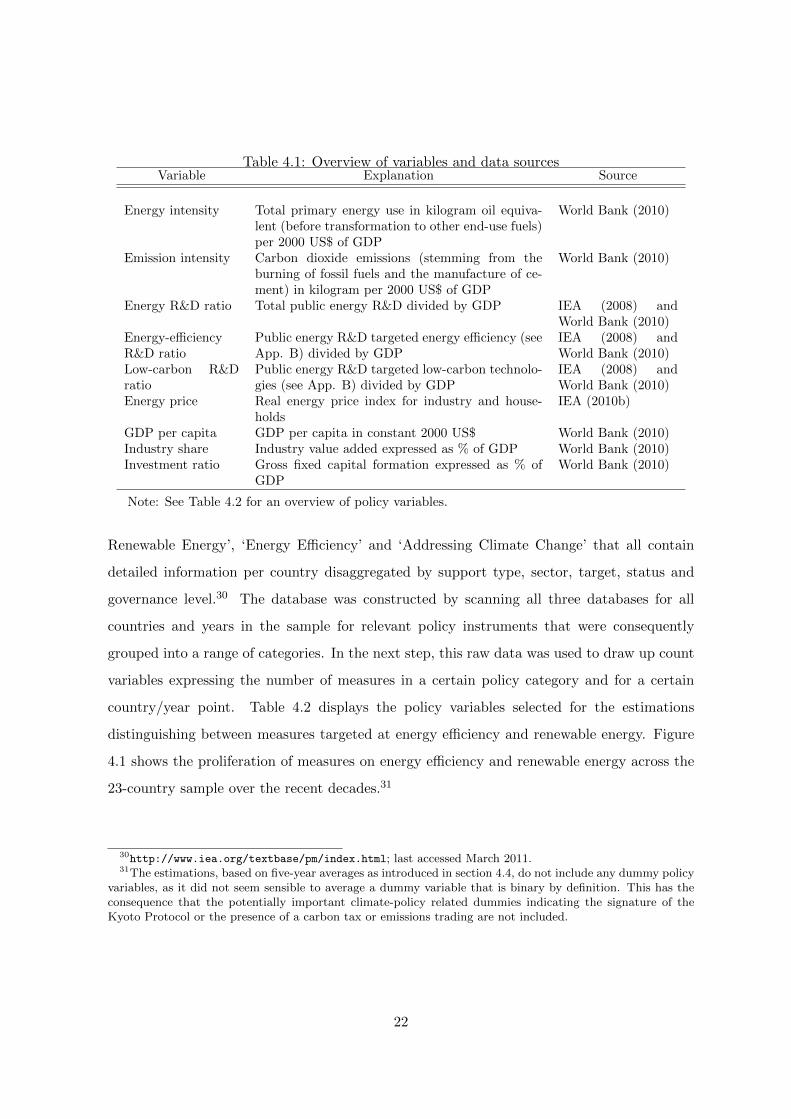
Table 4.1: Overview of variables and data sourcesVariable Explanation Source
Energy intensity Total primary energy use in kilogram oil equiva-lent (before transformation to other end-use fuels)per 2000 US$ of GDP
World Bank (2010)
Emission intensity Carbon dioxide emissions (stemming from theburning of fossil fuels and the manufacture of ce-ment) in kilogram per 2000 US$ of GDP
World Bank (2010)
Energy R&D ratio Total public energy R&D divided by GDP IEA (2008) andWorld Bank (2010)
Energy-efficiencyR&D ratio
Public energy R&D targeted energy efficiency (seeApp. B) divided by GDP
IEA (2008) andWorld Bank (2010)
Low-carbon R&Dratio
Public energy R&D targeted low-carbon technolo-gies (see App. B) divided by GDP
IEA (2008) andWorld Bank (2010)
Energy price Real energy price index for industry and house-holds
IEA (2010b)
GDP per capita GDP per capita in constant 2000 US$ World Bank (2010)Industry share Industry value added expressed as % of GDP World Bank (2010)Investment ratio Gross fixed capital formation expressed as % of
GDPWorld Bank (2010)
Note: See Table 4.2 for an overview of policy variables.
Renewable Energy’, ‘Energy Efficiency’ and ‘Addressing Climate Change’ that all contain
detailed information per country disaggregated by support type, sector, target, status and
governance level.30 The database was constructed by scanning all three databases for all
countries and years in the sample for relevant policy instruments that were consequently
grouped into a range of categories. In the next step, this raw data was used to draw up count
variables expressing the number of measures in a certain policy category and for a certain
country/year point. Table 4.2 displays the policy variables selected for the estimations
distinguishing between measures targeted at energy efficiency and renewable energy. Figure
4.1 shows the proliferation of measures on energy efficiency and renewable energy across the
23-country sample over the recent decades.31
30http://www.iea.org/textbase/pm/index.html; last accessed March 2011.31The estimations, based on five-year averages as introduced in section 4.4, do not include any dummy policy
variables, as it did not seem sensible to average a dummy variable that is binary by definition. This has theconsequence that the potentially important climate-policy related dummies indicating the signature of theKyoto Protocol or the presence of a carbon tax or emissions trading are not included.
22
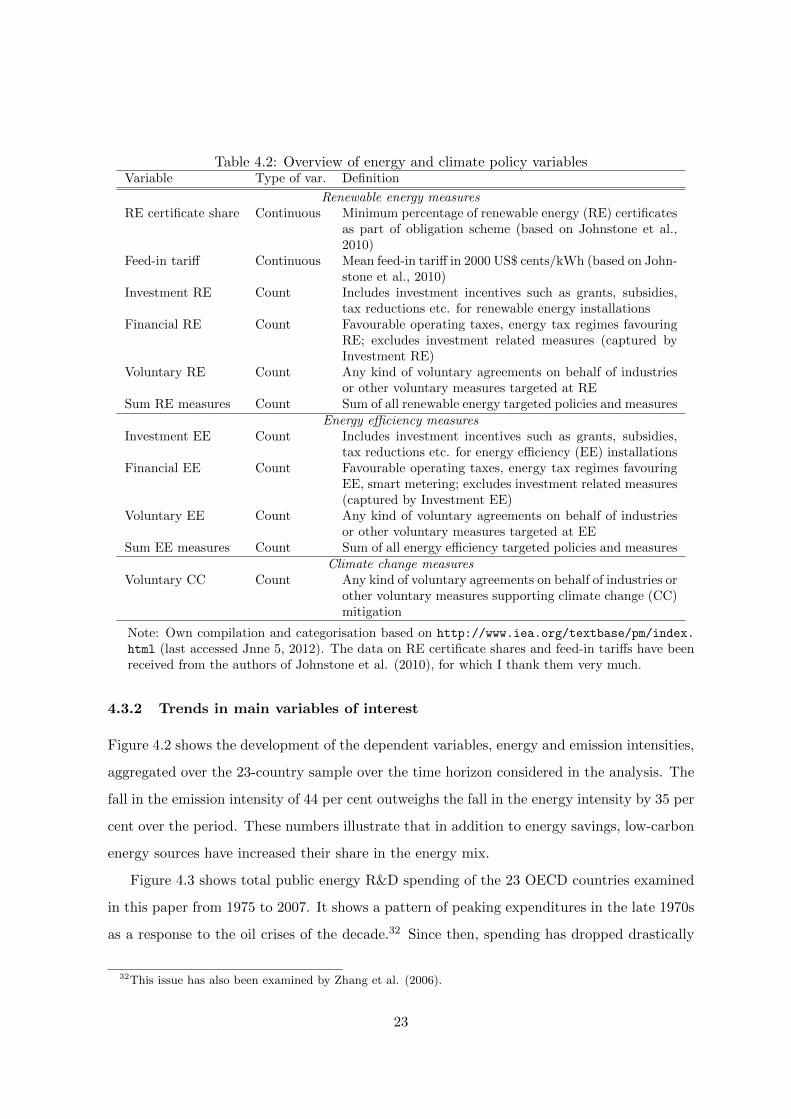
Table 4.2: Overview of energy and climate policy variablesVariable Type of var. Definition
Renewable energy measuresRE certificate share Continuous Minimum percentage of renewable energy (RE) certificates
as part of obligation scheme (based on Johnstone et al.,2010)
Feed-in tariff Continuous Mean feed-in tariff in 2000 US$ cents/kWh (based on John-stone et al., 2010)
Investment RE Count Includes investment incentives such as grants, subsidies,tax reductions etc. for renewable energy installations
Financial RE Count Favourable operating taxes, energy tax regimes favouringRE; excludes investment related measures (captured byInvestment RE)
Voluntary RE Count Any kind of voluntary agreements on behalf of industriesor other voluntary measures targeted at RE
Sum RE measures Count Sum of all renewable energy targeted policies and measuresEnergy efficiency measures
Investment EE Count Includes investment incentives such as grants, subsidies,tax reductions etc. for energy efficiency (EE) installations
Financial EE Count Favourable operating taxes, energy tax regimes favouringEE, smart metering; excludes investment related measures(captured by Investment EE)
Voluntary EE Count Any kind of voluntary agreements on behalf of industriesor other voluntary measures targeted at EE
Sum EE measures Count Sum of all energy efficiency targeted policies and measuresClimate change measures
Voluntary CC Count Any kind of voluntary agreements on behalf of industries orother voluntary measures supporting climate change (CC)mitigation
Note: Own compilation and categorisation based on http://www.iea.org/textbase/pm/index.
html (last accessed Jnne 5, 2012). The data on RE certificate shares and feed-in tariffs have beenreceived from the authors of Johnstone et al. (2010), for which I thank them very much.
4.3.2 Trends in main variables of interest
Figure 4.2 shows the development of the dependent variables, energy and emission intensities,
aggregated over the 23-country sample over the time horizon considered in the analysis. The
fall in the emission intensity of 44 per cent outweighs the fall in the energy intensity by 35 per
cent over the period. These numbers illustrate that in addition to energy savings, low-carbon
energy sources have increased their share in the energy mix.
Figure 4.3 shows total public energy R&D spending of the 23 OECD countries examined
in this paper from 1975 to 2007. It shows a pattern of peaking expenditures in the late 1970s
as a response to the oil crises of the decade.32 Since then, spending has dropped drastically
32This issue has also been examined by Zhang et al. (2006).
23
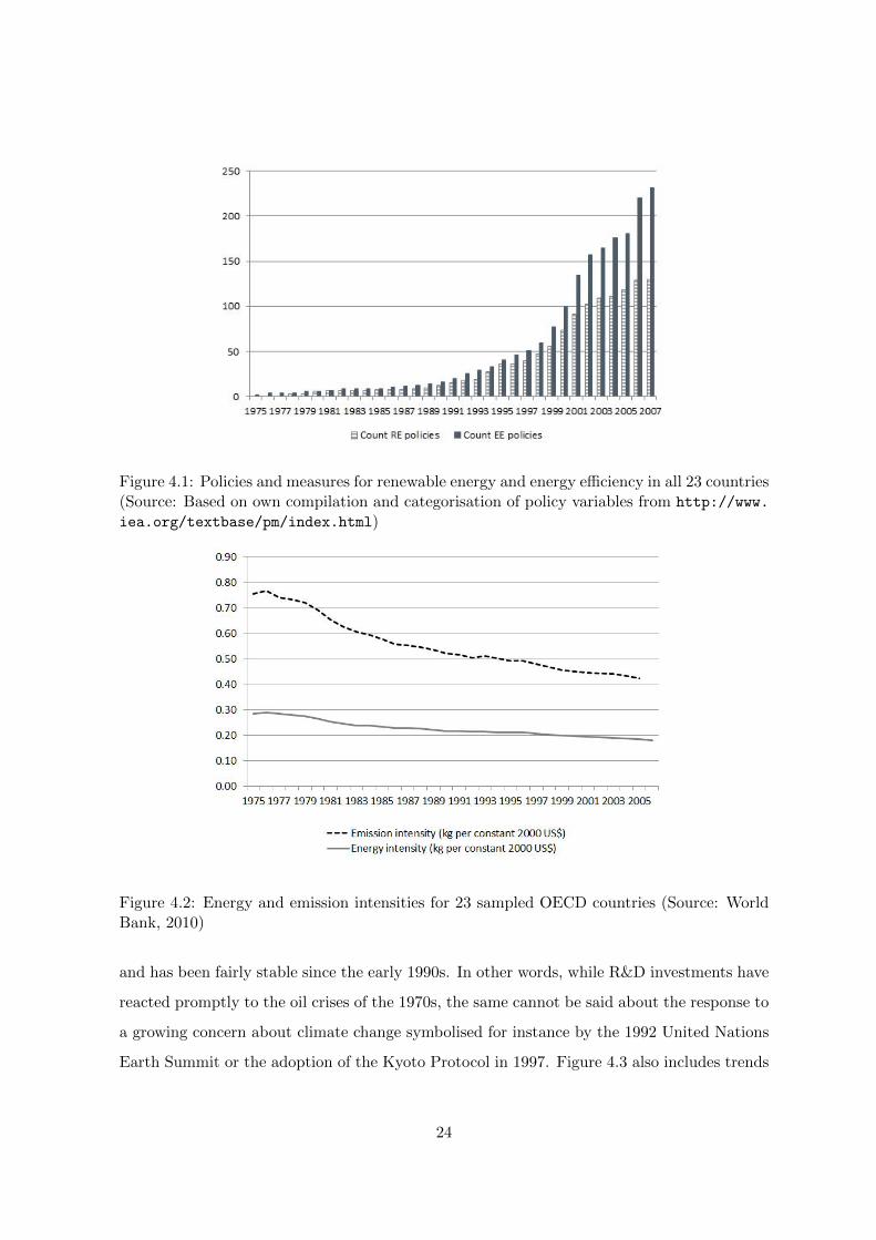
Figure 4.1: Policies and measures for renewable energy and energy efficiency in all 23 countries(Source: Based on own compilation and categorisation of policy variables from http://www.
iea.org/textbase/pm/index.html)
Figure 4.2: Energy and emission intensities for 23 sampled OECD countries (Source: WorldBank, 2010)
and has been fairly stable since the early 1990s. In other words, while R&D investments have
reacted promptly to the oil crises of the 1970s, the same cannot be said about the response to
a growing concern about climate change symbolised for instance by the 1992 United Nations
Earth Summit or the adoption of the Kyoto Protocol in 1997. Figure 4.3 also includes trends
24
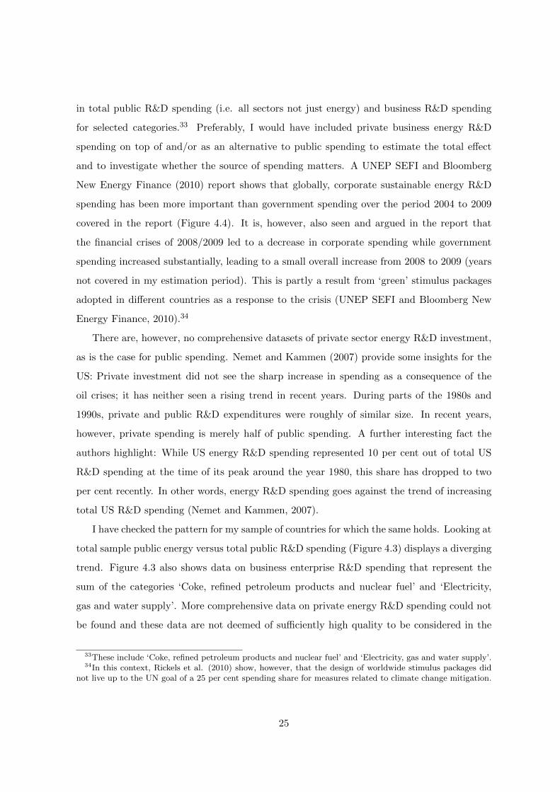
in total public R&D spending (i.e. all sectors not just energy) and business R&D spending
for selected categories.33 Preferably, I would have included private business energy R&D
spending on top of and/or as an alternative to public spending to estimate the total effect
and to investigate whether the source of spending matters. A UNEP SEFI and Bloomberg
New Energy Finance (2010) report shows that globally, corporate sustainable energy R&D
spending has been more important than government spending over the period 2004 to 2009
covered in the report (Figure 4.4). It is, however, also seen and argued in the report that
the financial crises of 2008/2009 led to a decrease in corporate spending while government
spending increased substantially, leading to a small overall increase from 2008 to 2009 (years
not covered in my estimation period). This is partly a result from ‘green’ stimulus packages
adopted in different countries as a response to the crisis (UNEP SEFI and Bloomberg New
Energy Finance, 2010).34
There are, however, no comprehensive datasets of private sector energy R&D investment,
as is the case for public spending. Nemet and Kammen (2007) provide some insights for the
US: Private investment did not see the sharp increase in spending as a consequence of the
oil crises; it has neither seen a rising trend in recent years. During parts of the 1980s and
1990s, private and public R&D expenditures were roughly of similar size. In recent years,
however, private spending is merely half of public spending. A further interesting fact the
authors highlight: While US energy R&D spending represented 10 per cent out of total US
R&D spending at the time of its peak around the year 1980, this share has dropped to two
per cent recently. In other words, energy R&D spending goes against the trend of increasing
total US R&D spending (Nemet and Kammen, 2007).
I have checked the pattern for my sample of countries for which the same holds. Looking at
total sample public energy versus total public R&D spending (Figure 4.3) displays a diverging
trend. Figure 4.3 also shows data on business enterprise R&D spending that represent the
sum of the categories ‘Coke, refined petroleum products and nuclear fuel’ and ‘Electricity,
gas and water supply’. More comprehensive data on private energy R&D spending could not
be found and these data are not deemed of sufficiently high quality to be considered in the
33These include ‘Coke, refined petroleum products and nuclear fuel’ and ‘Electricity, gas and water supply’.34In this context, Rickels et al. (2010) show, however, that the design of worldwide stimulus packages did
not live up to the UN goal of a 25 per cent spending share for measures related to climate change mitigation.
25
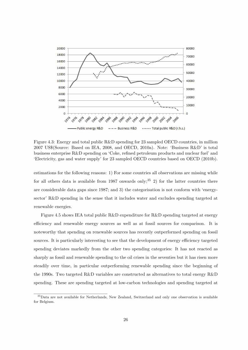
Figure 4.3: Energy and total public R&D spending for 23 sampled OECD countries, in million2007 US$(Source: Based on IEA, 2008, and OECD, 2010a). Note: ‘Business R&D’ is totalbusiness enterprise R&D spending on ‘Coke, refined petroleum products and nuclear fuel’ and‘Electricity, gas and water supply’ for 23 sampled OECD countries based on OECD (2010b).
estimations for the following reasons: 1) For some countries all observations are missing while
for all others data is available from 1987 onwards only;35 2) for the latter countries there
are considerable data gaps since 1987; and 3) the categorisation is not conform with ‘energy-
sector’ R&D spending in the sense that it includes water and excludes spending targeted at
renewable energies.
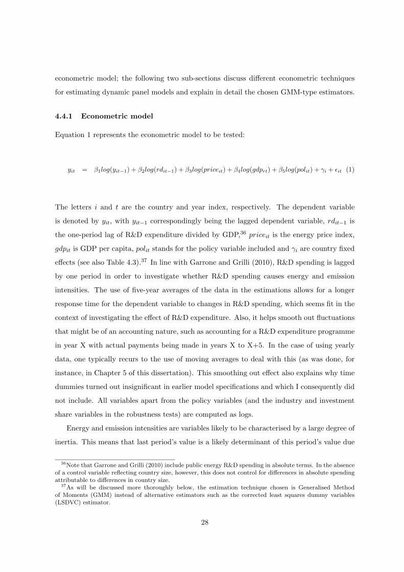
Figure 4.5 shows IEA total public R&D expenditure for R&D spending targeted at energy
efficiency and renewable energy sources as well as at fossil sources for comparison. It is
noteworthy that spending on renewable sources has recently outperformed spending on fossil
sources. It is particularly interesting to see that the development of energy efficiency targeted
spending deviates markedly from the other two spending categories: It has not reacted as
sharply as fossil and renewable spending to the oil crises in the seventies but it has risen more
steadily over time, in particular outperforming renewable spending since the beginning of
the 1990s. Two targeted R&D variables are constructed as alternatives to total energy R&D
spending. These are spending targeted at low-carbon technologies and spending targeted at
35Data are not available for Netherlands, New Zealand, Switzerland and only one observation is availablefor Belgium.
26
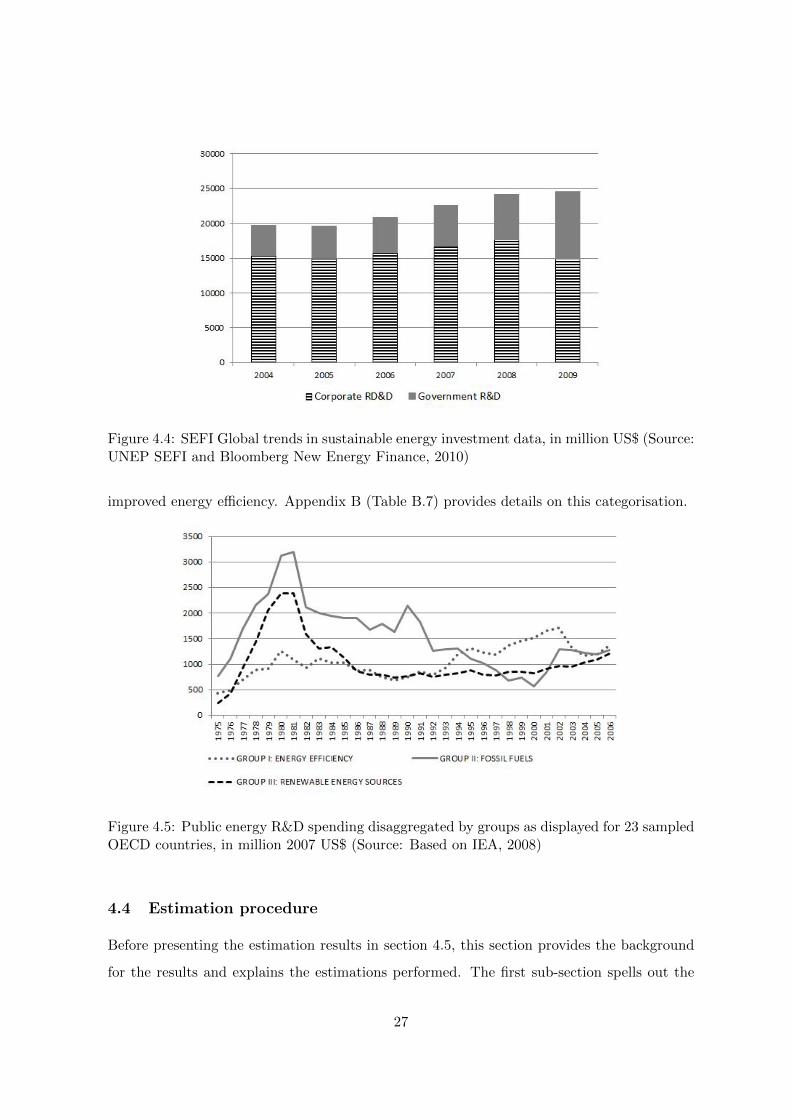
Figure 4.4: SEFI Global trends in sustainable energy investment data, in million US$ (Source:UNEP SEFI and Bloomberg New Energy Finance, 2010)
improved energy efficiency. Appendix B (Table B.7) provides details on this categorisation.
Figure 4.5: Public energy R&D spending disaggregated by groups as displayed for 23 sampledOECD countries, in million 2007 US$ (Source: Based on IEA, 2008)
4.4 Estimation procedure
Before presenting the estimation results in section 4.5, this section provides the background
for the results and explains the estimations performed. The first sub-section spells out the
27
econometric model; the following two sub-sections discuss different econometric techniques
for estimating dynamic panel models and explain in detail the chosen GMM-type estimators.
4.4.1 Econometric model
Equation 1 represents the econometric model to be tested:
yit = β1log(yit−1) + β2log(rdit−1) + β3log(priceit) + β4log(gdprt) + β5log(polit) + γi + εit (1)
The letters i and t are the country and year index, respectively. The dependent variable
is denoted by yit, with yit−1 correspondingly being the lagged dependent variable, rdit−1 is
the one-period lag of R&D expenditure divided by GDP,36 priceit is the energy price index,
gdpit is GDP per capita, polit stands for the policy variable included and γi are country fixed
effects (see also Table 4.3).37 In line with Garrone and Grilli (2010), R&D spending is lagged
by one period in order to investigate whether R&D spending causes energy and emission
intensities. The use of five-year averages of the data in the estimations allows for a longer
response time for the dependent variable to changes in R&D spending, which seems fit in the
context of investigating the effect of R&D expenditure. Also, it helps smooth out fluctuations
that might be of an accounting nature, such as accounting for a R&D expenditure programme
in year X with actual payments being made in years X to X+5. In the case of using yearly
data, one typically recurs to the use of moving averages to deal with this (as was done, for
instance, in Chapter 5 of this dissertation). This smoothing out effect also explains why time
dummies turned out insignificant in earlier model specifications and which I consequently did
not include. All variables apart from the policy variables (and the industry and investment
share variables in the robustness tests) are computed as logs.
Energy and emission intensities are variables likely to be characterised by a large degree of
inertia. This means that last period’s value is a likely determinant of this period’s value due
36Note that Garrone and Grilli (2010) include public energy R&D spending in absolute terms. In the absenceof a control variable reflecting country size, however, this does not control for differences in absolute spendingattributable to differences in country size.
37As will be discussed more thoroughly below, the estimation technique chosen is Generalised Methodof Moments (GMM) instead of alternative estimators such as the corrected least squares dummy variables(LSDVC) estimator.
28
to structural factors in the economy and the energy sector that do not change drastically from
one year to the next as a response to short term market signals. This justifies the inclusion of
the lagged dependent variable, which at the same time introduces challenges for estimation as
it biases OLS estimation. The next sections lay out the strategy to deal with these challenges.
Table 4.3: Overview of variable definitionsVariable Parameter values and definitions
YEnergy intensity (energy consumption / GDP)Emission intensity (emissions / GDP)
rdEnergy R&D ratio: Total public energy R&D spending / GDPEnergy-efficiency R&D ratio: Public R&D spending targeted at energy use/ GDP (see App. B)Low-carbon R&D ratio: Public R&D spending targeted at reducing emis-sions / GDP (see App. B)
pol Various policy variables as introduced in section 4.3.1
4.4.2 Estimation in the presence of endogenous regressors
The inclusion of the lagged dependent variable introduces a bias in the setting of a fixed time
dimension T . This bias derives from the fact that in panel OLS estimations employing fixed or
random effects, or first differencing, the lagged dependent variable exhibits contemporaneous
correlation with the error term or in other words is an endogenous regressor. The following
shortly introduces panel estimators focusing on the fixed effects and first difference estimator
and demonstrates where the bias originates and then introduces IV and GMM techniques as
the preferred way of eliminating the bias in the present setting.38
A main strength of the different panel estimators is that they deal with time-invariant
unobserved heterogeneity between individuals39 that are likely to be correlated with observed
explanatory variables in a panel data set. A standard example for time-invariant unobserved
heterogeneity is the inherent ability of individuals, for example of employees or students when
trying to explain differences in wages or test results, where ability is likely to be correlated
with ‘years of education’ or ‘hours studied’, respectively. In a macro panel, unobserved
heterogeneity includes country-specific characteristics such as long-standing and non-changing
38The introduction to estimation in the presence of endogenous regressors and to GMM estimation in thissection is primarily informed by Kennedy (2008) and Greene (2003).
39I.e. the cross section dimension of the data, ‘individuals’ in the present case being countries whereas inmicro panels typically individuals or firms make up the cross section.
29
(at least not over the sample period) cultural traditions or characteristics including geography
(e.g. land-locked) and climate conditions. Arguably, the latter can be observed and hence
could be included, however, the way in which both the fixed effects and the first difference
estimator deal with unobserved heterogeneity does not allow for the inclusion of such time-
invariant variables, as will be seen in the following.40 Equations 2 and 3 show how the fixed
effects and first difference estimators, respectively, remove the unobserved heterogeneity from
the data. The fixed effects estimator subtracts from all individual observations their mean
value or in other words demeans the data, with the mean being the average of all observations
for cross section i across time T . This transformation removes the unobserved heterogeneity,
which does not change over time and therefore cancels out. The same occurs when the data
is first-differenced as shown in equation 3.
(yit − yi) = β1(yit−1 − yi) + β2(Xit − Xi) + (γi − γi) + (εit − εi) (2)
(yit − yit−1) = β1(yit−1 − yit−2) + β2(Xit −Xit−1) + (γi − γi) + (εit − εit−1) (3)
Given that yit−1 = β1yit−2+β2Xit−1+γi+εit−1, it is easily detectable that the common element
εit−1 present in both the differenced lagged dependent variable as well as the differenced error
term (the same holds for the demeaned fixed effects model) introduces contemporaneous
correlation between an explanatory variable and the error term, violating one of the standard
assumptions underlying the OLS estimator and hence introducing a bias.
Instrumental variable (IV) and Generalised Method of Moments (GMM) estimators have
been developed in order to deal with the bias of dynamic panel data models. An alternative
way of dealing with the dynamic panel bias is the corrected least squares dummy variable
estimator (LSDVC) proposed by Bruno (2005a), introduced briefly in the next section. Refer-
ring to the first-difference model in equation 3, the underlying idea of employing instrumental
variables to eliminate the dynamic panel bias is to use deeper lags of the dependent variable in
40Time-invariant variables can be included in the random effects estimator due to a different derivation ofthis estimator. However, an underlying assumption of the random effects estimator is that the unobservedheterogeneity is uncorrelated with other explanatory variables, an assumption difficult to meet in many contextsincluding the examples just mentioned.
30
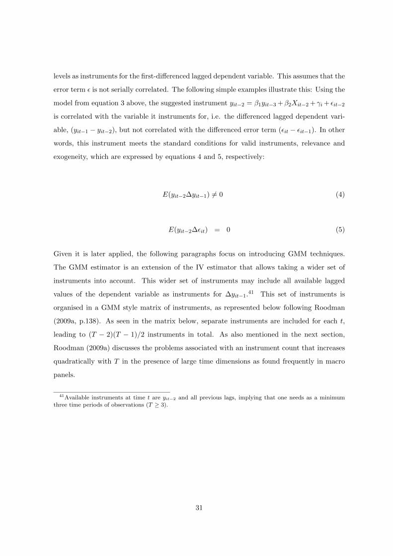
levels as instruments for the first-differenced lagged dependent variable. This assumes that the
error term ε is not serially correlated. The following simple examples illustrate this: Using the
model from equation 3 above, the suggested instrument yit−2 = β1yit−3 +β2Xit−2 + γi + εit−2
is correlated with the variable it instruments for, i.e. the differenced lagged dependent vari-
able, (yit−1 − yit−2), but not correlated with the differenced error term (εit − εit−1). In other
words, this instrument meets the standard conditions for valid instruments, relevance and
exogeneity, which are expressed by equations 4 and 5, respectively:
E(yit−2∆yit−1) 6= 0 (4)
E(yit−2∆εit) = 0 (5)
Given it is later applied, the following paragraphs focus on introducing GMM techniques.
The GMM estimator is an extension of the IV estimator that allows taking a wider set of
instruments into account. This wider set of instruments may include all available lagged
values of the dependent variable as instruments for ∆yit−1.41 This set of instruments is
organised in a GMM style matrix of instruments, as represented below following Roodman
(2009a, p.138). As seen in the matrix below, separate instruments are included for each t,
leading to (T − 2)(T − 1)/2 instruments in total. As also mentioned in the next section,
Roodman (2009a) discusses the problems associated with an instrument count that increases
quadratically with T in the presence of large time dimensions as found frequently in macro
panels.
41Available instruments at time t are yit−2 and all previous lags, implying that one needs as a minimumthree time periods of observations (T ≥ 3).
31
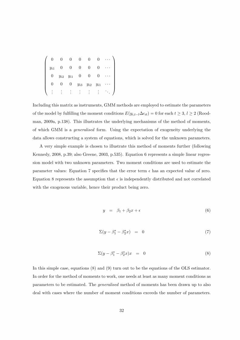
0 0 0 0 0 0 · · ·
yi1 0 0 0 0 0 · · ·
0 yi2 yi1 0 0 0 · · ·
0 0 0 yi3 yi2 yi1 · · ·...
......
......
.... . .
Including this matrix as instruments, GMM methods are employed to estimate the parameters
of the model by fulfilling the moment conditions E(yi,t−l∆εit) = 0 for each t ≥ 3, l ≥ 2 (Rood-
man, 2009a, p.138). This illustrates the underlying mechanisms of the method of moments,
of which GMM is a generalised form. Using the expectation of exogeneity underlying the
data allows constructing a system of equations, which is solved for the unknown parameters.
A very simple example is chosen to illustrate this method of moments further (following
Kennedy, 2008, p.39; also Greene, 2003, p.535). Equation 6 represents a simple linear regres-
sion model with two unknown parameters. Two moment conditions are used to estimate the
parameter values: Equation 7 specifies that the error term ε has an expected value of zero.
Equation 8 represents the assumption that ε is independently distributed and not correlated
with the exogenous variable, hence their product being zero.
y = β1 + β2x+ ε (6)
Σ(y − β∗1 − β∗2x) = 0 (7)
Σ(y − β∗1 − β∗2x)x = 0 (8)
In this simple case, equations (8) and (9) turn out to be the equations of the OLS estimator.
In order for the method of moments to work, one needs at least as many moment conditions as
parameters to be estimated. The generalised method of moments has been drawn up to also
deal with cases where the number of moment conditions exceeds the number of parameters.
32
In this case, not all moment conditions can be met and the parameter estimates are therefore
chosen to minimise the extent to which the total moment conditions are violated. After this
general introduction, the next section introduces different GMM estimators, focusing on the
specification used in the remainder of this paper.
4.4.3 Applying the GMM estimator to dynamic panels
This sub-section traces the development of applying the GMM estimator to dynamic panels
in general terms and then introduces its application in the context of the present analysis.
4.4.3.1 The general approach
A sizable body of econometric literature over the last decades has analysed the nature of the
bias introduced by the lagged dependent variable and developed estimation strategies to deal
with it, whose fundamentals the previous section introduced. Bruno (2005b) and Roodman
(2009b) provide overviews of the seminal papers and main estimators proposed. Anderson
and Hsiao (1982) introduced the IV-style estimator along the lines represented above. It first
transforms the model into first differences in order to eliminate unobserved cross-sectional
heterogeneity. The lagged dependent variable that is among the regressors is instrumented
by the second lag of the dependent variable either in levels or differenced form. Arellano
and Bond (1991) introduced the GMM estimator for the first-differenced model so as to use
additional internal instruments making it more efficient than Anderson and Hsiao’s estimator.
Blundell and Bond (1998) introduced a system GMM estimator that consists of a system of
one equation in levels containing first-differenced instruments and one equation in differences
containing levels instruments; the motivation underlying system GMM is to reduce a potential
small sample bias of IV and GMM estimators in the presence of highly persistent data.
With respect to the size of the bias, a seminal paper by Nickell (1981) has shown that
the bias is serious for small T and becomes less severe as T grows but has been shown
to still be significant with T as large as 30 (Judson and Owen, 1999). Attanasio et al.
(2000), on the other hand, advocate for considering simple OLS regressions given a “big
enough” time dimension. From their panel study comprising 38 to 123 countries and 24 to
34 years, they conclude that OLS estimators making use of T asymptotics are to be preferred
over instrumental variables (IV) techniques that have been designed for exploiting the N
33
asymptotics in micro panels because the higher precision of OLS outweighs the drawbacks of
the bias introduced by the lagged dependent variable.
Such evidence from Monte Carlo studies that cast doubt on the use of micro-econometric
methods in the context of macro panels provided a motivation for developing the LSDVC
estimator, proposed by Bruno (2005a) as an alternative way of dealing with the dynamic
panel bias. The LSDVC estimator is based on the standard, uncorrected least squares dummy
variable (LSDV) estimator, from which bias approximation estimates are subtracted. As
Bruno (2005b) explains, consistent initial estimators are needed for the calculation of these
bias approximation estimates42 Bruno (2005b) furthermore provides Monte Carlo evidence
comparing the different LSDVC estimators to the uncorrected LSDV and different GMM
estimators. According to both bias and root mean square error criteria, the LSDVC estimator
outperforms the others for samples with relatively few cross sections compared to their time
dimension (samples considered had cross-section to time dimensions of 20 to 20 and 10 to
40). Given that the cross-section dimension in the sample at hand is clearly larger than the
time dimension and for further reasons mentioned below, the preferred estimator employed
here is GMM.
4.4.3.2 Application in the present paper
Before spelling out the econometric details of the analysis, further arguments to mention in
favour of using GMM techniques in the present context are inconclusive unit root test results
for the main variables of interest employing the tests developed by Maddala and Wu (1999)
and Im et al. (2003). This could reduce the power of LSDVC estimations based on yearly
data but in the GMM estimations, the use of five-year averages erodes the basis for such
time-series concerns. The most important argument for using GMM estimation is, however,
the fact that R&D spending is likely to be endogenous and in fact has been demonstrated
as such in the analysis by Garrone and Grilli (2010). This approach is also in line with the
treatment of foreign aid as endogenous in regressions estimating the impact of aid on energy
and carbon intensities of developing economies in Kretschmer et al. (2013; also Chapter 5 of
this dissertation).
42The STATA routine xtlsdvc developed by Bruno (2005b) to implement the LSDVC estimator includes theGMM estimators by Anderson and Hsiao (1982), Arellano and Bond (1991) and Blundell and Bond (1998) asconsistent initial estimators.
34
One might question additionally whether policy variables are exogenous or whether the
levels of energy and carbon intensities actually determine policies. It can be safely argued,
however, that most renewable energy policies in advanced countries are enacted as a response
to a global concern, the threat of climate change, and can thus be considered exogenous.
Furthermore, measures that are a response to multilateral action (EU, UNFCCC) are unlikely
to be correlated with an individual country’s energy or emission intensities.43 They are hence
assumed exogenous variables in GMM estimations.
Some more specific remarks on the here chosen GMM techniques: I use the two-step
difference GMM estimator introduced by Arellano and Bond (1991) implemented in STATA
via the xtabond2 command written by Roodman (2009b). A main contribution of this com-
mand compared to the standard xtabond command is the inclusion of Windmeijer-corrected
standard errors for two-step estimation. The corrected standard errors by Windmeijer are im-
portant when it comes to using two-step GMM: As explained in Roodman (2009a), a singular
weighting matrix in two-step estimation is likely to occur when the number of instruments
approaches the number of cross sections. In that case, STATA makes use of the general-
ized matrix, which leaves the consistency of the parameter estimates unaffected but leads to
downward-biased standard errors. The advent of Windmeijer’s (2005) robust standard errors
reduces this problem. According to Roodman (2009b), making use of Windmeijer’s robust
standard errors renders two-step estimation superior to one-step estimation, with lower bias
and standard errors. With a larger T dimension and small cross-sectional dimension typical
for macro panels, the number of instruments included in the estimations, increasing quadrat-
ically in T , becomes a critical issue. A large instrument count is associated with weak Sargan
and Hansen J-tests that are used for testing the specification and more specifically the va-
lidity of instruments, frequently producing ‘perfect’ Hansen test-statistics of one (Roodman,
2009a). Given the limited number of time periods in the present setting due to the use of
five-year averages, excessive instrument counts do not arise and the full set of instruments
based on all available lags can be included.
43Rather, efforts taken by countries could be correlated with GDP per capita. However, Table B.4 inAppendix B does not reveal any serious multicollinearity between GDP per capita and policy count variablesand height of feed in tariffs and renewables obligations.
35
4.5 Estimation results
The first part of this section presents results for the original model specification as set out
above generated with GMM estimation techniques. The subsequent section presents results
for two separate robustness tests that introduce multiple policy variables and add control
variables. The final section discusses the results in light of other research.
4.5.1 Core GMM estimations
This section describes in detail the results from estimations with the overall energy R&D
ratio and the energy-efficiency targeted R&D ratio, as summarised in Tables 4.4 and 4.5,
respectively. Appendix C (Table C.1) reports results from estimations with R&D targeted
at low-carbon technologies. In these specifications, policy and R&D variables remain largely
insignificant and these estimations therefore do not yield many insights. Appendix C further
reports additional results focusing on voluntary measures in regressions with the energy in-
tensity on the left-hand side and including the different R&D spending variables (Table C.2).
In the following, I focus on Tables 4.4 and 4.5.
Turning to the description of the results: In all results tables, the numbering of specifica-
tions (column headings) indicates whether a certain specification includes the energy intensity
(E) or the emission intensity (C) as the dependent variable (the different specifications are
grouped into Panels A and B, respectively). Throughout the performed estimations, instru-
ments for the lagged differences of the dependent variable include all available lagged levels
of the dependent variable (from yit−2 onwards). The same holds for the R&D variables. The
test statistics demonstrate in most cases instrument validity as well as reasonable instrument
counts.
Looking at the results for the overall energy R&D ratio in Table 4.4: Energy R&D sig-
nificantly reduces energy intensity in specification E3 including the stringency of a renewable
energy obligation scheme. Given the log-linear model specification, coefficients can be in-
terpreted as elasticities: As an example, a one per cent increase in the energy R&D ratio
in specification E3 reduces the energy intensity by about 0.03 per cent; or put differently, a
doubling of R&D efforts (i.e. a 100 per cent increase) is needed to reduce the energy intensity
by about 3.2 per cent. Taking into account the coefficient of the lagged dependent variable,
36
the long-run effect of doubling R&D efforts can be calculated, amounting to 5.2 per cent.44
Energy R&D fails to reduce significantly energy intensity in the other specifications and nei-
ther reduces emission intensities. In some of the specifications with the energy intensity as
the dependent variable, the coefficient for energy R&D is close to significance at the 10 per
cent level (E1, E5 and E6). Even so, these results do not represent robust evidence for the
hypothesis that energy R&D spending reduces energy and emission intensities.
A further hypothesis put forward was that the significance and size of the effect of R&D
spending is conditional on the presence of demand-pull policies. There is, however, no ro-
bust increase in coefficients or t-statistics due to the inclusion of policy variables across the
different specifications. The one specification where energy R&D spending is significant is
E3 controlling for the stringency of a renewable energy obligation scheme, but this alone
cannot be interpreted as robust evidence supporting the hypothesis. Looking at the effect of
policies in their own right, Table 4.4 shows that in emission intensity specifications C4 and
C6 investment incentives for renewable energy and all renewable energy measures summed
together significantly reduce the emission intensity. This finding gives some support to the
hypothesis of expecting a reduction of the emission intensity in the presence of renewable
energy policies. However, also in the energy intensity specifications, it is renewable energy
rather than energy efficiency measures that display the highest t-statistics (feed-in tariff and
renewable energy investment support, i.e. specifications E2 and E4). The policy variables
targeting energy efficiency (E7 to E9 and C7 to C9) neither turn out significant nor influence
the effectiveness of R&D spending.
Looking at other control variables: The inertia in the lagged dependent variables is much
less pronounced than in unreported LSDVC regressions based on yearly data. While the
lagged energy intensity is highly significant, the lagged emission intensity is not significant.
GDP per capita robustly reduces energy and emission intensities and turns out highly signif-
icant in most specifications. This confirms the hypothesis that higher GDP per capita as a
proxy for productivity levels goes along with more energy efficient and cleaner technologies
and hence reduced energy and emission intensities. As an example, a one per cent increase
in GDP per capita leads to reductions in energy and emission intensities of up to 0.40 and
44This is calculated as β2/(1 − β1), where β1 and β2 are the coefficients of the lagged dependent variableand the R&D variable, respectively (see equation 1 above).
37
0.64 per cent, respectively. The energy price index generally reduces energy and emission
intensities, again confirming the previously formulated hypothesis that, all else equal, higher
energy prices make energy less and other factors of production more attractive hence reducing
an economy’s energy and (though to a less robust extent) emission intensity. The size of the
coefficients of the energy price index is generally smaller than the coefficients preceding GDP
per capita. Across all specifications in Table 4.4, the coefficients translate into a reduction of
the respective dependent variable of between 0.11 and 0.29 per cent for a one per cent increase
in the energy price index and a reduction between 0.22 and 0.64 per cent for a one per cent
increase in GDP per capita. It hence appears that the state of development of an economy
(as expressed by its GDP per capita level) is a more important determinant of energy and
emission intensities than the development of the energy price index.
Having said this, there are some anomalies in specifications E6 as well as C4, C6 and
C9, in the sense that the energy price index is no longer significant. In addition, no vari-
ables remain significant in specification E6. All of these specifications apart from C4 include
policy variables representing the count of all renewable energy or energy efficiency measures.
C4 includes the policy variable representing renewable energy investment incentives instead.
Several observations emerge that could form part of the explanation: In C4 and C6, the
respective policy variables are significant, potentially ‘taking away’ explanatory power of the
energy price index. In other words, it could be policy measures rather than energy price
signals that trigger the adoption of technologies that save energy and emissions.45 The same
does not hold for specifications E6 and C9, though t-statistics of the policy variables in those
specifications are higher than in some of the remaining ones. This observation is also valid for
Table 4.5 (and to a lesser extent for Table C.1, where the policy variable is only significant
in specification C4). Furthermore, the specifications scrutinised here are characterised by
rather low p-values of the Hansen J-test, a test for overall instrument validity. In particular,
the p-value of the Hansen test is lowest in E6 among all energy intensity specifications and
lowest for C4, C6 and C9 among all emission intensity specifications. This does not hold
in an equally robust way for Table 4.5. Nevertheless, at least the Hansen test statistic for
specification E6 is at the low end in Table 4.5.46 Weak instruments and hence a weaker model
45Though in a different context, this observation would be in line with the finding of Johnstone et al. (2010)that it is policies rather than prices that trigger innovation activity in the energy sector.
46This observation holds to some extent for Table C.1 as well, where the p-values for the Hansen test are
38
specification could form part of the explanation for the diverging results, though it is not clear
how this came about in the first place.
Turning to the results from estimations including R&D spending targeted at energy ef-
ficiency: Table 4.5 confirms the hypothesis that energy efficiency targeted R&D spending is
more likely to explain energy intensities than emission intensities and has greater explanatory
power than overall R&D spending. The R&D variable is significant in several specifications
including the baseline specification E1. However, total energy R&D spending (Table 4.4)
mostly displays larger coefficients in the energy intensity specifications. This is different in the
emission intensity specifications, where the coefficients of targeted R&D spending are higher
compared to those of overall R&D spending (though both are insignificant at conventional
levels). While energy efficiency targeted R&D spending is never significant in regressions with
the emission intensity as the dependent variable, in columns C2 to C9 (with the exception of
C5) both its coefficient and t-statistic increase in the presence of policies.
The largest significant effect of energy efficiency R&D spending is found in specification E3
(including the renewable energy certificate share): An increase in R&D spending of one per
cent reduces the energy intensity by 0.03 per cent, or in other words a rather small reduction
of 2.9 per cent results from a doubling of R&D spending. The long run effect is also highest
in specification E3 and equal to a reduction of 4.7 per cent for a doubling of R&D spending.
Focusing further on the left hand panel of Table 4.5, the presence and height of renewable
obligations strengthens the coefficient and t-statistic of R&D spending, as it did in Table 4.4
for the overall R&D spending ratio. The same holds for financial renewable energy incentives
and the sum of renewable energy measures (here the significance remains stable). In the
presence of investment incentives and the sum of energy efficiency measures, on the other
hand, R&D spending loses its significance. These results can be seen as some tentative, yet
mixed evidence supporting the hypothesis that the effectiveness of R&D spending increases
in the presence of policies. On the effect of the policy measures themselves: The results
are similar to those in Table 4.4: None of the policies is significant in the energy intensity
estimations but again renewable energy investment policies and the sum of all renewable
energy policies reduce emission intensities.
below or just above 0.10 in several specifications, indicating weak instruments and potentially explaining thelack of insights from these estimations.
39
Other control variables perform similarly as in Table 4.4. This also holds for the loss of
significance in the energy price index in specifications E6, C4, C6, C7 and C9. Potential
explanations have been proposed above already. Results for specification E6 are somewhat
different to the same specification in Table 4.4 in the sense that the lagged dependent variable
and R&D spending remain significant while GDP per capita and the energy price index turn
out insignificant.
A few remarks highlighting the main findings from the estimations summarised in Tables
C.1 and C.2 in Appendix C. As previously mentioned, Table C.1 shows that R&D spending
targeted at low-carbon technologies fails to reduce energy and emission intensities through-
out all specifications. Results for other variables are largely similar to what has been found
in estimations including the other R&D spending variables as discussed above. Turning to
Table C.2 in Appendix C focusing on voluntary measures: Somewhat surprisingly, while the
policy variables themselves all turn out insignificant, total R&D spending enters significantly
in energy-intensity estimations including voluntary measures targeted at renewable energy,
energy efficiency and climate mitigation, respectively. Energy-efficiency R&D remains signif-
icant in Columns E7 and E9 (renewables and climate voluntary measures). The same does
not hold for estimations with the emission intensity as the dependent variable.
Final remarks on the effect of the policy variables: Apart from what has been mentioned
in the previous paragraphs, I highlight the negative relationship between investment incen-
tives for renewable energy and the count of all renewable measures with emission intensities.
While not rendering R&D spending effective, their presence does increase the respective
coefficients of the R&D variables (and mostly their t-statistics as well). It is apparent that
energy efficiency measures do not turn out significant. This can be explained by energy
efficiency measures often being of a more soft nature without ‘hard’ and binding targets,
exemplified by the situation in the EU where binding renewable energy targets exist but no
equivalent for energy efficiency.
40
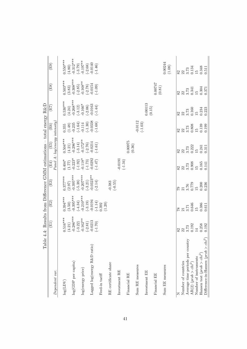
Tab
le4.4
:R
esu
lts
from
Diff
eren
ceG
MM
esti
mat
ion
s–
tota
len
ergy
R&
D(E
1)
(E2)
(E3)
(E4)
(E5)
(E6)
(E7)
(E8)
(E9)
Dep
end
ent
var.
Pa
nel
A:
log(
ener
gyin
ten
sity
)
log(L
DV
)0.5
16***
0.3
94***
0.3
77***
0.4
04*
0.5
04***
0.3
55
0.5
30***
0.5
03***
0.5
50***
(4.2
1)
(3.5
0)
(2.9
7)
(1.7
7)
(4.2
1)
(1.4
8)
(4.2
4)
(3.8
3)
(4.8
0)
log(G
DP
per
capit
a)
-0.2
86***
-0.3
95***
-0.3
95***
-0.2
23*
-0.2
96***
-0.2
35
-0.2
68***
-0.3
08***
-0.3
12***
(-3.2
2)
(-4.3
4)
(-5.3
8)
(-1.9
2)
(-3.1
4)
(-1.6
4)
(-3.1
2)
(-2.8
5)
(-3.7
9)
log(e
ner
gy
pri
ce)
-0.1
62**
-0.2
10***
-0.2
07***
-0.1
18*
-0.1
72**
-0.1
14
-0.1
66*
-0.1
68**
-0.1
97**
(-2.8
1)
(-3.1
9)
(-3.2
1)
(-1.7
3)
(-2.7
6)
(-1.3
0)
(-2.0
6)
(-2.7
8)
(-2.6
8)
Lagged
log(e
ner
gy
R&
Dra
tio)
-0.0
213
-0.0
194
-0.0
323**
-0.0
292
-0.0
214
-0.0
338
-0.0
163
-0.0
154
-0.0
140
(-1.7
0)
(-1.1
4)
(-2.1
4)
(-1.4
7)
(-1.6
1)
(-1.6
8)
(-1.4
4)
(-1.0
9)
(-1.4
6)
Fee
d-i
nta
riff
0.3
92
(1.2
0)
RE
cert
ifica
tesh
are
-0.3
83
(-0.5
5)
Inves
tmen
tR
E-0
.0191
(-1.3
4)
Fin
anci
al
RE
0.0
0975
(0.3
6)
Sum
RE
mea
sure
s-0
.0112
(-1.0
3)
Inves
tmen
tE
E0.0
0113
(0.1
5)
Fin
anci
al
EE
0.0
0747
(0.8
1)
Sum
EE
mea
sure
s0.0
0244
(1.0
8)
N82
78
79
82
82
82
82
82
82
Num
ber
of
countr
ies
22
21
21
22
22
22
22
22
22
Aver
age
tim
ep
erio
ds
per
countr
y3.7
33.7
13.7
63.7
33.7
33.7
33.7
33.7
33.7
3A
R(2
)(prob>chi2
)0.1
92
0.6
46
0.7
79
0.9
08
0.2
22
0.8
08
0.1
60
0.3
41
0.1
34
Num
ber
of
inst
rum
ents
14
15
15
15
15
15
15
15
15
Hanse
nte
st(prob>chi2
)0.2
58
0.3
86
0.2
00
0.1
65
0.2
41
0.1
39
0.2
34
0.3
04
0.3
48
Diff
eren
ce-i
n-H
anse
n(prob>chi2
)0.1
92
0.6
11
0.2
36
0.1
41
0.3
11
0.1
99
0.2
23
0.3
71
0.5
11
41

(C1)
(C2)
(C3)
(C4)
(C5)
(C6)
(C7)
(C8)
(C9)
Dep
end
ent
var.
Pa
nel
B:
log(
emis
sio
nin
ten
sity
)
log(L
DV
)0.1
66
0.1
49
0.1
23
0.1
43
0.1
40
0.0
879
0.1
43
0.1
70
0.1
01
(1.6
1)
(0.8
5)
(0.7
3)
(0.9
7)
(0.9
8)
(0.6
6)
(1.0
7)
(1.5
1)
(0.5
9)
log(G
DP
per
capit
a)
-0.5
86***
-0.6
40***
-0.6
42***
-0.4
88**
-0.6
12***
-0.4
80**
-0.5
87***
-0.5
77***
-0.5
57***
(-4.1
1)
(-4.1
3)
(-3.3
8)
(-2.3
6)
(-3.7
9)
(-2.4
0)
(-3.8
4)
(-4.2
7)
(-3.8
3)
log(e
ner
gy
pri
ce)
-0.2
47***
-0.2
87***
-0.2
40**
-0.1
42
-0.2
55**
-0.1
11
-0.2
06*
-0.2
43**
-0.1
60
(-3.0
7)
(-3.0
8)
(-2.2
6)
(-1.6
2)
(-2.5
4)
(-1.0
6)
(-1.9
3)
(-2.6
5)
(-1.2
5)
Lagged
log(e
ner
gy
R&
Dra
tio)
-0.0
128
-0.0
0543
-0.0
164
-0.0
153
-0.0
111
-0.0
234
-0.0
227
-0.0
147
-0.0
275
(-0.4
1)
(-0.1
7)
(-0.5
0)
(-0.4
3)
(-0.3
5)
(-0.6
2)
(-0.7
4)
(-0.4
7)
(-0.8
1)
Fee
d-i
nta
riff
0.5
12
(0.9
4)
RE
cert
ifica
tesh
are
-0.2
72
(-0.2
0)
Inves
tmen
tR
E-0
.0205*
(-2.0
5)
Fin
anci
al
RE
0.0
0115
(0.0
2)
Sum
RE
mea
sure
s-0
.0162*
(-1.7
9)
Inves
tmen
tE
E-0
.00572
(-0.5
5)
Fin
anci
al
EE
-0.0
0733
(-0.2
1)
Sum
EE
mea
sure
s-0
.00505
(-1.0
8)
N80
76
77
80
80
80
80
80
80
Num
ber
of
countr
ies
22
21
21
22
22
22
22
22
22
Aver
age
tim
ep
erio
ds
per
countr
y3.6
43.6
23.6
73.6
43.6
43.6
43.6
43.6
43.6
4A
R(2
)(prob>chi2
)0.2
83
0.2
92
0.2
82
0.3
22
0.2
75
0.4
16
0.3
36
0.2
93
0.3
37
Num
ber
of
inst
rum
ents
14
15
15
15
15
15
15
15
15
Hanse
nte
st(prob>chi2
)0.2
08
0.1
18
0.1
47
0.1
02
0.1
99
0.0
94
0.1
64
0.2
23
0.1
33
Diff
eren
ce-i
n-H
anse
n(prob>chi2
)0.6
78
0.6
38
0.8
15
0.7
74
0.4
73
0.7
31
0.7
21
0.8
43
0.9
52
Note
:t
stati
stic
sin
pare
nth
eses
;*p<
0.1
0,
**p<
0.0
5,
***p<
0.0
1***;
LD
Vden
ote
sla
gged
dep
enden
tva
riable
42
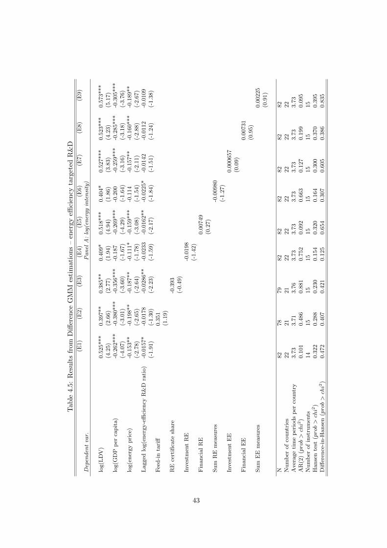
Tab
le4.5
:R
esu
lts
from
Diff
eren
ceG
MM
esti
mat
ion
s–
ener
gyeffi
cien
cyta
rget
edR
&D
(E1)
(E2)
(E3)
(E4)
(E5)
(E6)
(E7)
(E8)
(E9)
Dep
end
ent
var.
Pa
nel
A:
log(
ener
gyin
ten
sity
)
log(L
DV
)0.5
25***
0.3
97**
0.3
85**
0.4
09*
0.5
18***
0.4
04*
0.5
27***
0.5
23***
0.5
73***
(4.2
5)
(2.6
6)
(2.7
7)
(1.9
4)
(4.9
4)
(1.8
6)
(3.8
3)
(4.2
3)
(5.1
7)
log(G
DP
per
capit
a)
-0.2
62***
-0.3
80***
-0.3
56***
-0.1
87
-0.2
69***
-0.2
00
-0.2
59***
-0.2
85***
-0.3
05***
(-4.0
7)
(-3.0
1)
(-3.6
0)
(-1.6
7)
(-4.2
9)
(-1.6
4)
(-3.1
6)
(-3.1
8)
(-3.7
6)
log(e
ner
gy
pri
ce)
-0.1
53**
-0.1
98**
-0.1
87**
-0.1
11*
-0.1
59***
-0.1
14
-0.1
57**
-0.1
60***
-0.1
89**
(-2.7
8)
(-2.6
5)
(-2.6
4)
(-1.7
8)
(-3.0
8)
(-1.5
4)
(-2.1
1)
(-2.8
8)
(-2.6
7)
Lagged
log(e
ner
gy-e
ffici
ency
R&
Dra
tio)
-0.0
157*
-0.0
178
-0.0
286**
-0.0
233
-0.0
162**
-0.0
225*
-0.0
142
-0.0
112
-0.0
109
(-1.9
1)
(-1.3
0)
(-2.2
3)
(-1.5
9)
(-2.1
7)
(-1.8
4)
(-1.5
1)
(-1.2
4)
(-1.3
8)
Fee
d-i
nta
riff
0.3
51
(1.1
9)
RE
cert
ifica
tesh
are
-0.3
93
(-0.4
9)
Inves
tmen
tR
E-0
.0198
(-1.4
2)
Fin
anci
al
RE
0.0
0749
(0.2
7)
Sum
RE
mea
sure
s-0
.00980
(-1.2
7)
Inves
tmen
tE
E0.0
00657
(0.0
9)
Fin
anci
al
EE
0.0
0731
(0.9
5)
Sum
EE
mea
sure
s0.0
0225
(0.9
1)
N82
78
79
82
82
82
82
82
82
Num
ber
of
countr
ies
22
21
21
22
22
22
22
22
22
Aver
age
tim
ep
erio
ds
per
countr
y3.7
33.7
13.7
63.7
33.7
33.7
33.7
33.7
33.7
3A
R(2
)(prob>chi2
)0.1
01
0.4
86
0.8
81
0.7
52
0.0
92
0.6
63
0.1
27
0.1
99
0.0
95
Num
ber
of
inst
rum
ents
14
15
15
15
15
15
15
15
15
Hanse
nte
st(prob>chi2
)0.3
22
0.2
88
0.2
30
0.1
54
0.3
20
0.1
64
0.3
00
0.3
70
0.3
95
Diff
eren
ce-i
n-H
anse
n(prob>chi2
)0.4
72
0.4
07
0.4
21
0.1
25
0.6
54
0.3
07
0.6
05
0.3
86
0.8
35
43
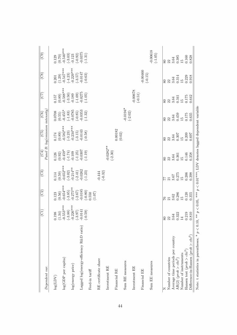
(C1)
(C2)
(C3)
(C4)
(C5)
(C6)
(C7)
(C8)
(C9)
Dep
end
ent
var.
Pa
nel
B:
log(
emis
sio
nin
ten
sity
)
log(L
DV
)0.1
98
0.1
23
0.1
14
0.1
26
0.1
74
0.0
708
0.1
57
0.2
01
0.1
29
(1.3
4)
(0.5
6)
(0.5
9)
(0.9
2)
(0.8
9)
(0.5
5)
(0.8
9)
(1.2
9)
(0.7
0)
log(G
DP
per
capit
a)
-0.5
53***
-0.6
54***
-0.6
52***
-0.4
59*
-0.5
82***
-0.4
55*
-0.5
88***
-0.5
47***
-0.5
40***
(-3.8
8)
(-3.8
5)
(-3.0
2)
(-1.7
4)
(-3.2
3)
(-1.8
3)
(-3.5
0)
(-4.2
3)
(-3.0
3)
log(e
ner
gy
pri
ce)
-0.2
26***
-0.2
75**
-0.2
14**
-0.1
09
-0.2
34***
-0.0
785
-0.1
89
-0.2
29***
-0.1
23
(-3.9
7)
(-2.6
7)
(-2.4
1)
(-1.2
5)
(-3.1
5)
(-0.8
5)
(-1.6
9)
(-3.5
7)
(-0.9
2)
Lagged
log(e
ner
gy-e
ffici
ency
R&
Dra
tio)
-0.0
141
-0.0
185
-0.0
262
-0.0
307
-0.0
143
-0.0
353
-0.0
275
-0.0
147
-0.0
375
(-0.5
9)
(-0.8
0)
(-1.2
3)
(-1.1
9)
(-0.5
8)
(-1.3
2)
(-1.0
5)
(-0.6
3)
(-1.3
1)
Fee
d-i
nta
riff
0.5
50
(1.0
7)
RE
cert
ifica
tesh
are
-0.4
44
(-0.3
2)
Inves
tmen
tR
E-0
.0282**
(-2.3
0)
Fin
anci
al
RE
0.0
0182
(0.0
2)
Sum
RE
mea
sure
s-0
.0194*
(-2.0
2)
Inves
tmen
tE
E-0
.00678
(-0.5
1)
Fin
anci
al
EE
-0.0
0460
(-0.1
5)
Sum
EE
mea
sure
s-0
.00618
(-1.0
5)
N80
76
77
80
80
80
80
80
80
Num
ber
of
countr
ies
22
21
21
22
22
22
22
22
22
Aver
age
tim
ep
erio
ds
per
countr
y3.6
43.6
23.6
73.6
43.6
43.6
43.6
43.6
43.6
4A
R(2
)(prob>chi2
)0.3
22
0.2
86
0.2
75
0.3
61
0.3
07
0.4
59
0.3
41
0.3
14
0.3
85
Num
ber
of
inst
rum
ents
14
15
15
15
15
15
15
15
15
Hanse
nte
st(prob>chi2
)0.2
19
0.1
20
0.2
06
0.1
46
0.2
09
0.1
75
0.1
75
0.2
29
0.1
60
Diff
eren
ce-i
n-H
anse
n(prob>chi2
)0.8
10
0.3
55
0.3
98
0.3
58
0.6
97
0.6
35
0.6
42
0.9
18
0.8
28
Note
:t
stati
stic
sin
pare
nth
eses
;*p<
0.1
0,
**p<
0.0
5,
***p<
0.0
1***;
LD
Vden
ote
sla
gged
dep
enden
tva
riable
44
4.5.2 Robustness checks
A first robustness test includes multiple policies. It could be argued that this is a more
realistic setting as policies targeted at different energy variables frequently coexist in the real
world. Policies were included one by one in the main regressions above in order to understand
better the effect of individual policies. Table C.3 in Appendix C reports the results. Results
on R&D variables are robust to the inclusion of multiple policy variables. Where total R&D
was significant in energy intensity estimations, it remains so with further policies accounted
for (Panel A). Robust, however, also means that the performance of R&D spending in emission
intensity estimations does not improve and remains insignificant throughout. The same holds
for the estimations including energy efficiency targeted R&D in Panel B of Table C.3. One
observation to point out is that the inclusion of multiple policy variables tends to rather
increase than decrease the t-statistics of the R&D variable, comparing for instance columns
(C4) and (C6) in Table C.3 to column (C3) in Table 4.5. Results are furthermore robust for
estimations including R&D spending targeted at low-carbon technologies (Panel C).
Another robustness check includes additional control variables to the econometric
model. I start out by adding industrial value added as a share of GDP. As in Kretschmer et
al. (2013) this serves to capture changes in the composition of the economy acknowledging
that the industrial sector is likely to be more energy intensive than activities in the agricultural
and services sector. In another set of estimations, I include the investment ratio (gross fixed
capital formation as a percentage of GDP). Enhanced investment activity could lead to a more
rapid replacement of the capital stock and thus could imply a shift towards a more efficient
production structure. This is at least an effect that would be expected for OECD countries,
where industrialisation has generally started prior to the beginning of our estimation period in
1976 hence subsequent investment is likely to indeed renew the existing capital stock instead
of newly introducing energy-intensive industry, which could be associated with higher energy
and emission intensities. I finally include both the industry share and the investment ratio in
the estimations.
It turns out that the previous results are sensitive to accounting for changes in the sec-
toral structure of the economies and more importantly for investment. The significance of
R&D spending and of policy variables remains in some of the estimations involving the indus-
try share, but not in all. This is even though the industry share itself remains insignificant
45
throughout.47 R&D spending is insignificant in all emission intensity estimations as before,
however, here the inclusion of the industry share increases coefficients (they mostly decrease
in energy intensity regressions) as well as t-statistics, which remain low nevertheless. The
inclusion of the investment ratio influences results more significantly (see Table C.4). Invest-
ment as a share of GDP displays a significant negative relationship with energy intensity while
it is insignificant (but also negative) in emission intensity estimations. When accounting for
investment, R&D spending is never significant anymore. Including both the investment ratio
and the industry share simultaneously implies that the investment ratio is no longer significant
in most cases. As before, R&D spending and most policy variables are insignificant.
4.5.3 The results in perspective
This section serves to put the results reported in the previous sections into the context of
related studies. Similar to the results that this study arrived at, Garrone and Grilli (2010) find
that energy R&D spending influences the energy efficiency but not the emission intensities of
a sample of OECD economies. R&D spending targeted at energy efficiency and low-carbon
technologies does not alter this pattern in either study. These results hold across the two
studies despite the difference in the data set: Garrone and Grilli work with a smaller data set of
13 countries spanning 25 years compared to 23 countries and 31 years in the present analysis.
They also hold despite the differences in defining the R&D variables. While the present
analysis uses R&D to GDP ratios in order to control for the size of the economies, Garrone
and Grilli (2010) use absolute R&D spending in their bivariate analysis, hence leaving country
size uncontrolled. This latter difference implies that a comparison between sizes of coefficients
in the two studies is meaningless. Garrone and Grilli (2010) offer additional results on reverse
causality and point out that both the emission and energy intensities positively granger-
cause energy R&D spending. They consequently interpret that “energy R&D budgeting is
critically exposed to political pressure [. . . ] and consequently deserves greater monitoring and
evaluation efforts” (p.5610).
47On the sign of the (albeit insignificant) coefficients: The industry share is largely preceded by a negativesign in energy-intensity estimations (unlike what was expected) while its sign is largely positive in emission-intensity estimations. This changes when I take into account the investment ratio simultaneously; in theseestimations, the industry share, while still remaining insignificant throughout, turns positive in almost allestimations for both dependent variables.
46
Similar to the present results though in a different context, Kretschmer et al. (2013) find
that foreign aid has some power to reduce energy intensities of developing economies but fails
to reduce the carbon intensity of energy supply, i.e. the carbon factor. While the developing-
country context is arguably specific and among others goes along with utterly different energy
mixes, the studies offer similar explanations for this pattern of results. Garrone and Grilli
(2010) point out that the inability of energy R&D to influence emission intensities is due
to its inability to influence the carbon factor. Unreported regressions undertaken in the
present analysis confirm this inability. Garrone and Grilli (2010) explain this with the greater
uncertainty of research programmes targeted at low-carbon technologies, “a field where the
design of policies complementary to public energy R&D is especially challenging” (p.5607)
and “accompanying measures (i.e. policies oriented to diffusion and deployment, a sharper
design of energy R&D budgets, a continuous assessment of research programmes” (p.5610)
are crucial alongside R&D investment. Likewise, Kretschmer et al. note that the “incentives
for emission savings could be strengthened through a carbon price, and possibly also through
a better targeting of financial and technological assistance” (2013, p.86).
As mentioned earlier, some of the policy variables have been adopted from Johnstone et
al. (2010). Given the different research question at hand in their study (the impact of R&D
expenditure and renewable energy policies on patent applications for different low-carbon
technologies), a comparison between their results and those generated here is hardly possible.
An interesting result from their study is that “policy, rather than prices, appears to be the
main driver of innovation” in low-carbon technologies (p.146). In other words, their market
related variables electricity price and growth of electricity consumption turn out insignificant.
This is different to the present results. In the context of economy-wide energy and carbon
intensities, market factors such as the energy price index as well as economic development as
represented by GDP per capita play a very important role. Their dominant role is likely to
explain some of the failure to detect longer-term effects from energy R&D spending, a result
that extends the bivariate analysis by Garrone and Grilli (2010).
As their analysis is disaggregated according to different low-carbon technologies, John-
stone et al. (2010) can furthermore identify differences in the impacts of renewable energy
policies on different technologies. They find that the effectiveness of policies depends on the
relative cost of a technology: As an example, renewable energy targets, a measure that usu-
47
ally does not distinguish between technologies, favour low-cost technologies while specifically
designed feed-in tariffs allow for innovation in high-cost technologies as well. While this exact
distinction is not relevant in the context at hand, the concluding section stresses the merits
of a more disaggregated analysis.
4.6 Conclusions
This paper empirically analyses the effect of energy R&D spending on energy and emission
intensities in OECD countries, accounting for the presence of policies targeted at renewable
energy, energy efficiency and climate change. I find some evidence for energy R&D spending
to reduce energy intensities but not emission intensities in the 23 OECD countries considered
and over the years 1977 to 2006. The negative effect on energy intensities is primarily found
in estimations using energy-efficiency targeted R&D spending whose effect becomes stronger
and/or more significant in the presence of renewable energy policy measures. R&D spending
targeted at low-carbon technologies shows negative coefficients throughout but fails to pass
conventional significance levels in all estimations.
A focus of the analysis was whether the inclusion of policy measures targeted at energy and
climate outcomes would improve the effectiveness of R&D spending according to theoretical
work that technology-push measures such as R&D spending would need to be accompanied
by market creation policies. In some instances, the introduction of policy variables does
indeed render R&D spending significant (or increases t-statistics without R&D becoming
significant) and/or increases the size of its coefficients. While this provides some empirical
evidence supporting the theoretical work on the interplay of technology-push and demand-
pull measures, this result is not robust across all estimations. Another conclusion is that it
was almost exclusively policies targeted at renewable energy wielding this effect, such as the
minimum percentage of renewable energy certificates as part of obligation schemes, investment
and other financial incentives for renewables and the sum of all renewable energy measures.
Surprisingly, while voluntary measures remained largely insignificant, their presence made the
reducing effect of the total R&D spending ratio on energy intensities significant in a robust
way.
Speaking of the significance of policy measures themselves, it is again renewable energy
measures rather than energy efficiency measures that turn out significant, especially the al-
48
ready mentioned minimum percentage of renewable energy certificates as part of obligation
schemes, investment incentives and the sum of all renewable energy measures. Speaking of fur-
ther control variables, both GDP per capita and energy prices show a largely robust negative
relationship with energy and emission intensities. The lagged dependent variable is significant
in energy intensity estimations but not in estimations explaining emission intensities.
The results prove to be largely robust to including multiple policy measures in the regres-
sions. They turned out to be sensitive, however, to the inclusion of the industry share and
more so of the investment ratio. This second robustness check could be interpreted as point-
ing out the difficulty of using R&D spending as an explanatory variable in an econometric
analysis because of its long lead times in having an effect whereas the effect of investment in
capital formation is much easier to detect.
Future research could be undertaken to tackle the present failure of providing more com-
pelling evidence for the effectiveness of R&D spending in the presence of policy measures.
Given the availability of a fine disaggregation of public R&D spending data according to
individual objectives and technologies, the obvious next step would be to also have sectoral
data on the left hand side of the estimations. In that way, one could try, for instance, to
explain the effect of energy efficiency spending targeted at the residential sector on the en-
ergy performance of buildings in the presence of policy measures supporting energy efficient
renovation. Likewise, the emission intensity of the power sector would be an obvious choice
for a sectoral dependent variable. The lack of precision of an aggregate, country-level analysis
as the present one is all the more relevant in a context where policy variables are used, which
might be very targeted in nature and only applicable to narrow sectors. While the approach
of counting the number of measures under one category has been put forward as a way of
at least capturing the variety of measures applied to all sectors in one policy variable, the
policy variables here are unweighted sums of measures. Subsequent analysis could improve
this aspect by weighting policies according to the size of the sector they are targeted at and
the budgeted size of the policy, where applicable.
Another limitation concerning the construction of the policy variables database is a de-
gree of inherent subjectivity or impreciseness associated with allocating policies to different
categories. In addition, the databases used for the construction of policy variables give no
indication about the effectiveness in implementing the policy measures and so aspects such as
49
poor management of certain policy measures cannot be captured by assigning them a lower
weight.
Finally, the availability of longer time series would allow covering the most recent years,
a period that was at least in EU countries characterised by the emergence of much more
coherent sets of policy measures to foster renewable energy as a response to the obligations
imposed by the Renewable Energy Directive.48 It will hence be interesting to see whether
R&D spending can be demonstrated to be more effective in the presence of a closer network
of market creation policies in the future.
48Reporting on the progress made by Member States, the Commission states that the introduction of bindingtargets has triggered a pronounced increase in the efforts made by Member States. Communication COM(2011)31 final from the Commission to the European Parliament and the Council of 31 January 2011: RenewableEnergy: Progressing towards the 2020 target.
50
5 Does Foreign Aid Reduce Energy and Carbon Intensities of
Developing Economies?49
Full citationBettina Kretschmer, Michael Hubler, Peter Nunnenkamp, Does foresign aid reduce energyand carbon intensities of developing economies?, Journal of International Development,Volume 25, Issue 1, January 2013, Pages 67-91, ISSN 1099-1328, DOI: 10.1002/jid.1788.
Permanent link: http://dx.doi.org/10.1002/jid.1788
JEL classification: F35; Q41; Q55Keywords: Energy intensity; CO2 emissions; Foreign aid; Developing countries
AbstractAdvanced OECD countries are widely held responsible for containing global carbon emissionsby providing financial and technical support to developing economies where emissions areincreasing most rapidly. It is open to question, however, whether more generous official de-velopment assistance would help fight climate change effectively. Empirical evidence on theeffects of foreign aid on energy and carbon emission intensities in recipient countries hardlyexists. We contribute to closing this gap by considering energy use and carbon emissionsas dependent climate-related variables and the volume and structure of aid as possible deter-minants. In particular, we assessed the impact of aid that donors classify to be specificallyrelated to energy issues. We performed dynamic panel Generalised Method of Moments andLeast Squares Dummy Variable Corrected estimations. We found that aid tends to be effec-tive in reducing the energy intensity of GDP in recipient countries. All the same, the carbonintensity of energy use is hardly affected. Scaling up aid efforts would thus be insufficient tofight climate change beyond improving energy efficiency.
49This Chapter has been written jointly with Michael Hubler (now Centre for European Economic Research,ZEW) and Peter Nunnenkamp (Kiel Institute for the World Economy). An identical version (apart from somesmall edits and layout changes) is published in the Journal of Intenational Development as Kretschmer et al.(2013). We would like to thank Michaela Rank and Stephan Baier for most helpful assistance in collecting thedata. Several colleagues provided kind support and advice with respect to methods and data issues, includingAxel Dreher, Holger Gorg, Matthias Hartmann, Dierk Herzer and Sebastian Petrick. My contribution wasto help in spelling out the econometric model; to do most of the data collection and preparation; to devisethe estimation strategy, especially with regard to the choice of appropriate estimators (with advice from myco-authors); to perform all estimations; and to contribute to the interpretation and writing up of results.
51
6 Conclusions
The research conducted in the framework of this dissertation contributes to the evidence
base on the effect of different policies including biofuel support mechanisms, public energy
R&D spending and foreign aid on the decarbonisation of energy supply. In particular, the
analyses have responded primarily to three key research questions derived from the energy-
climate nexus and the twin challenges of securing energy supply while decarbonising our
economies. These are 1) understanding the macroeconomic impacts of promoting energy-
saving and low-carbon technologies, here the impacts of promoting EU biofuel use up to the
year 2020; 2) understanding the effectiveness of public support mechanisms in decarbonising
economies, here the effectiveness of past public energy R&D spending in the presence of energy
and climate policies in OECD countries; and 3) understanding the way in which developed
countries can contribute to decarbonising the economies of developing countries by means of
foreign aid.
The analyses presented here are examples of both ex-ante (Chapters 2 and 3) and ex-
post (Chapters 4 and 5) policy evaluation. Both forms of policy evaluation are important to
draw lessons for designing effective policy measures and also to understand and eventually
mitigate potential unintended side effects. EU policy in the field of biofuels is a good example
for highlighting this need for evidence-based policy-making: ex-ante analyses were either not
(well) conducted or not considered and have consequently failed to highlight the inherent risks
the policy entails in terms of increased land use competition, land use emissions and higher
agricultural commodity prices.
Chapter 2 has reviewed different ways of modelling biofuel technologies in economic
CGE models, aiming to contribute to the ongoing improvements in models that will in turn
allow for better ex-ante modelling of the effects of policies. It distinguished three types of
biofuel modelling approaches, an “implicit approach”, a “latent technology approach” and
an approach consisting of disaggregating the underlying data structure of CGE models, the
social accounting matrix. The studies reviewed yield a wide range of results, suggesting
that crucial assumptions need to undergo continued ‘reality checks’ to narrow this range.
Further improvements in modelling were expected to be made with better data availability
and in fact this and considerable attention and resources devoted to the modelling of biofuel
policies have advanced the research considerably over the past years since the time of writing.
52
Especially the land use components of economic models have improved, an improvement need
that was particularly stressed by Kretschmer and Peterson (2010). Another improvement
still outstanding is the modelling of second-generation biofuel technologies that make use
of a broader feedstock basis (including for example forest and agricultural residues). These
biofuels are hoped to reduce some of the negative impacts of first-generation biofuels, most
notably (indirect) land use change and associated emissions, but in fact, their potential to
do so is as of yet neither well understood nor studied. Even so, there are calls from industry
and civil society for specific support measures for these fuels, which goes against the aim of
gathering the evidence before adopting policy measures.
Chapter 3 built on an extended version of the CGE model DART to analyse the economic
effects of a 10 per cent biofuel blending share in the EU in different scenarios including emission
mitigation targets and varying shares of renewable electricity. Given assumed technology
cost parameters and the development of carbon prices (endogenous in DART), it was found
that EU emission targets alone trigger only minor increases in biofuel production as biofuel
technologies remain largely uncompetitive making targeted subsidies necessary to reach a
10 per cent biofuel share. One focus of the analysis were the agricultural market impacts
and in particular the impacts on commodity prices. Significant price effects were found with
average EU agricultural sector prices increasing by up to 7 per cent in the biofuel scenarios
in 2020 compared to a reference scenario (up to 3.5 per cent for world agricultural prices).
The results of the welfare analysis yield the interesting observation of lower welfare losses,
compared to the reference scenario, in a scenario with a 10 per cent biofuel and a moderate
renewable electricity share than in a scenario with no biofuel target but a higher (30 per cent)
renewable electricity share. However, it also concluded that in the presence of biofuel targets
worldwide, greater distortionary effects from biofuel promotion leading to larger welfare losses
as well as larger increases in world agricultural prices would be expected. A policy implication
that emerges from this paper is the need for a better understanding of the cost-effectiveness
and welfare implications of the renewable energy mix especially when thinking about future,
higher renewable energy targets. Such analysis needs to take into account the actual amount
of emissions saved by different renewable options. This is especially relevant in the case of
bioenergy and its associated land use and land use change emissions.
The analysis of the impact of energy R&D spending in OECD countries in Chapter 4
53
yields some evidence of energy R&D spending having been effective in reducing energy but
not emission intensities. The further disaggregation of energy R&D spending shows that the
negative effect on energy intensities is primarily found in estimations using energy-efficiency
targeted R&D spending. This effect becomes stronger and/or more significant in the presence
of renewable energy policy measures. R&D spending targeted at low-carbon technologies
has not significantly reduced energy or carbon intensities. Some, but no robust empirical
evidence was found supporting the importance of demand-pull measures for R&D spending
to be effective as suggested by theoretical work. Where policies have increased the size or
significance of the effect of R&D on energy intensities, these were almost exclusively renewable
energy and not energy efficiency policies. Future research that would readdress the questions
within a sectoral analysis would be useful for refining the results reached here. The result
that renewable energy measures are found to be better suited to enhance or allow for the
effectiveness of R&D spending suggests that energy efficiency considerations need to figure
more prominently in energy policy making. This, for instance, could result in the adoption
of energy efficiency targets along with renewable energy targets.
The analysis of foreign aid to reduce energy and carbon intensities in developing economies
(Chapter 5) suggested a modest contribution of total aid inflows to reducing energy intensi-
ties in recipient countries. On the other hand, aid did not turn out to be effective in reducing
carbon intensities. Sectoral aid data were used accounting for aid targeted at the energy and
the industrial sector. The main results for total aid also hold for energy aid, while aid for
the industrial sector turns out to be ineffective. The main caveat of the results relates to
the fungibility of aid or in other words the potential that recipients may redirect domestic
funds away from the energy sector as a consequence of donors targeting this sector, which
could (partly) explain the lack of effectiveness of foreign aid to improve energy and carbon
intensities. The small contribution of aid inflows to reducing energy intensities suggests that
policy makers both in recipient and donor countries should conceive of aid as complementing
domestic (i.e. recipient countries’) policies for improving energy efficiency and preventing
wasteful use of energy (as for instance triggered by fossil fuel subsidies). Policy making could
strengthen the incentive for emission savings through the introduction of carbon pricing and
better targeting of financial and technological assistance, for example in the framework of
the Green Climate Fund. The fact that energy sector aid leaves the results qualitatively
54
unchanged calls for a more targeted approach of rigorously redirecting aid to renewable en-
ergy and energy efficiency funding and/or even identifying concrete projects with large and
cost-effective energy and emission saving potentials.
The continued analysis of different mechanisms to foster renewable energy deployment
and reduce energy and carbon intensities is important, especially given the continued failure
to reach a binding international agreement to contain climate change. In the meantime and
in parallel to the top-down, multilateral UNFCCC process, individual countries and regions
such as the EU have imposed or are in the process of imposing decarbonisation targets. This
suggests a gradual shift towards a bottom-up approach to climate change mitigation (see
for instance Carraro and Egenhofer, 2007). In the time until 2020 when a global agreement
is hopefully agreed and operationalised, domestic climate and energy policy, including the
elements studied in this dissertation, will be crucial to avoid carbon lock-in effects due to
carbon-intensive investments in emerging economies. The results of the research presented
here ideally contribute to the design of effective policy measures facilitated by a better under-
standing of anticipated impacts as well as by monitoring their effectiveness once implemented.
55
References
Anderson, T. W. and C. Hsiao (1982). Formulation and Estimation of Dynamic ModelsUsing Panel Data. Journal of Econometrics 18(1), 47–82.
Arellano, M. and S. Bond (1991). Some Tests of Specification for Panel Data: Monte CarloEvidence and an Application to Employment Equations. Review of Economic Studies 58(2), 277–297.
Attanasio, O.P., L. Picci and A.E. Scorcu (2000). Saving, Growth, and Investment: AMacroeconomic Analysis Using a Panel of Countries. Review of Economics and Statistics82(2), 182–211.
Blundell, R. and S. Bond (1998). Initial Conditions and Moment Restrictions in DynamicPanel Data Models. Journal of Econometrics 87(1), 115–143.
Bruno, G.S.F. (2005a). Approximating the Bias of the LSDV Estimator for DynamicUnbalanced Panel Data Models. Economics Letters 87(1), 361–366.
Bruno, G.S.F. (2005b). Estimation and Inference in Dynamic Unbalanced Panel DataModels with a Small Number of Individuals. Stata Journal 5(4), 473–500.
Carraro, C. and C. Egenhofer (eds.) (2007). Climate and Trade Policy: Bottom-upApproaches Towards Global Agreement. ESRI studies series on the environment. EdwardElgar, Cheltenham, USA and Northhampton, USA.
Edwards, R., Mulligan, D. and Marelli, L. (2010). Indirect Land Use Change from increasedbiofuels demand: Comparison of models and results for marginal biofuels production fromdifferent feedstocks. JRC Scientific and Technical Reports, European Commission JointResearch Centre, Institute for Energy, Ispra, Italy.
Enkvist, P.A., T. Naucler and J. Rosander (2007). A cost curve for greenhouse gas reduction.The McKinsey Quarterly 1, 34–45.
EREC and Greenpeace (2010). Energy[r]evolution: Towards a Fully Renewable EnergySupply in the EU 27. http://www.energyblueprint.info/fileadmin/media/documents/
national/2010/0910_gpi_E_R__eu_report_4_lr.pdf (last accessed January 22, 2012).
Fischer, C. (2008). Emissions pricing, spillovers, and public investment in environmentallyfriendly technologies. Energy Economics 30, 487–502.
Fischer, C. and R.G. Newell (2008). Environmental and technology policies for climatemitigation. Journal of Environmental Economics and Management 55, 142–162.
Fischer, G. (2011). How can climate change and the development of bioenergy alter thelong-term outlook for food and agriculture? In: Conforti, P. (Ed.) Looking ahead in world
56
food and agriculture: Perspectives to 2050. Food and Agriculture Organization of the UnitedNations, Rome, Italy.
Garrone, P. and L. Grilli (2010). Is there a relationship between public expenditures inenergy R&D and carbon emissions per GDP? An empirical investigation. Energy Policy 38,5600–5613.
Greene, W. H. (2003) (5th ed.). Econometric Analysis. Upper Saddle River, NJ [and others]:Prentice-Hall.
Grubb, M. (2004). Technology Innovation and Climate Change Policy: An Overview ofissues and Options. Keio Economic Studies 41(2), 103–132.
Hertel, T. W., Tyner, W. E. and Birur, D. K. (2010). Global Impacts of Biofuel Mandates.Energy Journal 31(1), 75-100.
IEA (2008). Energy Technology RD&D budgets database (2008 edition). InternationalEnergy Agency, Paris, France.
IEA (2010). Energy Prices and Taxes Statistics, IEA online database (3rd quarter 2010edition). International Energy Agency, Paris, France.
Im, K. S., M. H. Pesaran, and Y. Shin (2003). Testing for unit roots in heterogeneous panels.Journal of Econometrics 115, 53–74.
IPCC (2000). Summary for Policy Makers. In: IPCC Special Report Emissions Scenarios [N.Nakicenovic and R. Swart (eds.)], Cambridge University Press, Cambridge, United Kingdom.
IPCC (2007). Climate Change 2007: Synthesis Report of the Fourth Assessment Report ofthe Intergovernmental Panel on Climate Change. Cambridge University Press, Cambridge,UK, and New York, NY, USA.
IPCC (2011). Summary for Policymakers. In: IPCC Special Report on Renewable EnergySources and Climate Change Mitigation [O. Edenhofer, R. Pichs-Madruga, Y. Sokona, K.Seyboth, P. Matschoss, S. Kadner, T. Zwickel, P. Eickemeier, G. Hansen, S. Schlomer, C.von Stechow (eds.)], Cambridge University Press, Cambridge, United Kingdom and NewYork, NY, USA.
IPCC (2012). Summary for Policymakers. In: Managing the Risks of Extreme Events andDisasters to Advance Climate Change Adaptation [Field, C.B., V. Barros, T.F. Stocker, D.Qin, D.J. Dokken, K.L. Ebi, M.D. Mastrandrea, K.J. Mach, G.-K. Plattner, S.K. Allen,M. Tignor, and P.M. Midgley (eds.)]. A Special Report of Working Groups I and II of theIntergovernmental Panel on Climate Change. Cambridge University Press, Cambridge, UK,and New York, NY, USA, pp. 3-21.
Johnstone, N., I. Hascic and D. Popp (2010). Renewable Energy Policies and TechnologicalInnovation: Evidence Based on Patent Counts. Environmental and Resource Economics 45,
57
133–155.
Judson, R.A. and A.L. Owen (1999). Estimating Dynamic Panel Data Models: A Guide forMacroeconomists. Economic Letters 65(1), 9–15.
Kennedy, P. (2008) (6th ed.). A guide to econometrics. Malden, MA [and others]: Blackwell.
Klepper, G., S. Peterson and K. Springer (2003). DART97: A Description of the Multi-regional, Multi-sectoral Trade Model for the Analysis of Climate Policies. Kiel WorkingPaper 1149, Kiel Institute for the World Economy, Kiel, Germany.
Klepper, G. and S. Peterson (2007). Distribution Matters - Taxes vs. Emissions Tradingin Post-Kyoto Climate Regimes. Kiel Working Paper 1380, Kiel Institute for the WorldEconomy, Kiel, Germany.
Kretschmer, B., M. Hubler and P. Nunnenkamp (2013). Does Foreign Aid Reduce Energyand Carbon Intensities of Developing Economies? Journal of International Development 25,67-91.
Kretschmer, B., D. Narita and S. Peterson (2009). The economic effects of the EU biofueltarget. Energy Economics 31, S285–S294.
Kretschmer, B. and S. Peterson (2010). Integrating Bioenergy into Computable GeneralEquilibrium Models – A Survey. Energy Economics 32, 673–686.
Kretschmer, B., S. Peterson and A. Ignaciuk (2008). Integrating biofuels into the DARTmodel. Kiel Working Paper 1472, Kiel Institute for the World Economy, Kiel, Germany.
Maddala, G.S. and S. Wu (1999). A Comparative Study of Unit Root Tests With PanelData and A New Simple Test. Oxford Bulletin of Economics and Statistics 61, 631–652.
Nemet, G.F. and D.M. Kammen (2007). U.S. energy research and development: Declininginvestment, increasing need, and the feasibility of expansion. Energy Policy 35, 746–755.Data online: https://mywebspace.wisc.edu/nemet/web/RandD2006.html (last accessedJune 5, 2012).
Nickell, S.J. (1981). Biases in Dynamic Models with Fixed Effects. Econometrica 49(6),1417–1426.
OECD (2010a). OECD.Stat Gross Domestic Expenditure on R-D by sector of performanceand type of cost. Organisation for Economic Co-Operation and Development, Paris,France: http://stats.oecd.org/OECDStat_Metadata/ShowMetadata.ashx?Dataset=
GERD_COST&ShowOnWeb=true&Lang=en (last accessed May 2011).
OECD (2010b). OECD.Stat Business enterprise R-D expenditure by industry and bysource of funds. Organisation for Economic Co-Operation and Development, Paris,France: http://stats.oecd.org/OECDStat_Metadata/ShowMetadata.ashx?Dataset=
58
BERD_FUNDS&ShowOnWeb=true&Lang=en (last accessed May 2011).
OECD-IEA (2011). World Energy Outlook 2011 – Executive Summary. International EnergyAgency, Paris, France.
O’Hare, M., M. Delucchi, R. Edwards, U. Fritsche, H. Gibbs, T. Hertel, J. Hill, D. Kammen,D. Laborde, L. Marelli, D. Mulligan, R. Plevin and W. Tyner (2011). Comment on ”Indirectland use change for biofuels: Testing predictions and improving analytical methodologies”by Kim and Dale: statistical reliability and the definition of the indirect land use change(iLUC) issue. Biomass and Bioenergy 35(10), 4485-4487.
Raupach, M. R., G. Marland, P. Ciais, C. Le Qur, J. G. Canadell, G. Klepper and C. B.Field (2007). Global and Regional Drivers of Accelerating CO2 Emissions. Proceedings ofthe National Academy of Sciences (PNAS) 104(24), 10288–10293.
Rickels, W., L. Kleemann, G. Klepper, S. Peterson and S. Petrick (2010). Konjunkturfur den Klimaschutz? Klima- und Wachstumswirkung weltweiter Konjunkturprogramme.Aussenwirtschaft 2010 II, Universitat St. Gallen.
Roodman, D. (2009a). A Note on the Theme of Too Many Instruments. Oxford Bulletin ofEconomics and Statistics 71(1), 135–158.
Roodman, D. (2009b). How to do xtabond2: an introduction to difference and system GMMin Stata. Stata Journal 9(1), 86–136.
Sagar, A.D. and B. van der Zwaan (2006). Technological innovation in the energy sector:R&D, deployment, and learning-by-doing. Energy Policy 34, 2601–2608.
UNEP SEFI and Bloomberg New Energy Finance (2010). Global Trends in SustainableEnergy Investment 2010: Analysis of Trends and Issues in the Financing of RenewableEnergy and Energy Efficiency, http://sefi.unep.org/english/globaltrends2010.html
(last accessed June 5, 2012).
World Bank (2010). World Development Indicators. Washington, D.C., USA.
World Bank (2011). World Development Indicators. Washington, D.C., USA.
WWF and Ecofys (2011). The Energy Report: 100% Renewable Energy by 2050.www.panda.org/energyreport (last accessed June 5, 2012).
Zhang, J.-T. Y. Fan and Y-M. Wei (2006). An empirical analysis for national energy R&Dexpenditures. International Journal of Global Energy Issues 25(1-2), 141–159.
59
Appendices
A The integration of biofuel technologies in the DART model
The integration of biofuel technologies in the computable general equilibrium (CGE) model
DART forms the basis for the simulations in Chapter 3 of this dissertation. The way in
which we integrated biofuel technologies including the disaggregation of GTAP sectors to
introduce new sectors and all associated data collection and changes to the model’s structure
are described in detail in Kretschmer et al. (2008). General features of the DART model
are not repeated here, given they are introduced in Kretschmer et al. (2009) (Chapter 3).
Kretschmer et al. (2009) furthermore explain the general procedure of introducing biofuels in
DART as latent technologies. Here I focus on some more detailed aspects of the integration
of the new production sectors, i.e. the production structure in the new sectors compared
to the production structure in the original DART sectors and the way in which biofuels
are included on the consumption side of the model while at the same time presenting the
choice of important parameters. The following summary is informed both by Kretschmer et
al. (2008) as well as Klepper et al. (2003), the latter describing the standard DART model
without biofuels, on which we built.
Biofuel production
Bioethanol and biodiesel can be produced from different agricultural feedstocks (sugar cane
and beet, wheat and corn for bioethanol and different oilseeds and vegetable oil for biodiesel).
The shares of the respective feedstock and other inputs such as capital, labour and electric-
ity were determined on the basis of industry data provided by meo Consulting Team (as
shown in Table 2 of Kretschmer et al., 2009). The production structures in both biofuel
and other sectors in the DART model are described by multi-level nested constant elasticity
of substitution (CES) functions. Figure A.1 shows the production structure in the biofuel
sectors which translates into a corresponding MPSGE code, the ‘mathematical programming
system for general equilibrium analysis’ (developed by Rutherford, 1987) within the GAMS
programming language in which the DART model is written. At the top level, the feedstock
input, electricity and a value added composite of capital and labour are connected by a Leon-
60
tief function, i.e. are modelled as perfect complements with an elasticity of substitution of
zero. The fact that the agricultural feedstock as the raw material is the dominant input in
biofuel production justifies the lack of substitution potential. In the lower level nests, capital
and labour form the value added composite described by a Cobb-Douglas function with an
elasticity of substitution of one as in the standard DART model (Klepper et al., 2003) and
as commonly found in CGE models. Both feedstock and electricity inputs can be either im-
ported or domestically produced. In line with the Armington assumption commonly employed
in CGE models, imported and domestic goods are considered heterogeneous goods and are
hence imperfect substitutes (accounting for example for a home bias of consumers). Given
the global market for the agricultural commodities wheat, corn and vegetable oils (as well as
for gasoline and other refined oil products), a higher Armington elasticity of substitution of
8 as opposed to 4 for all remaining goods is chosen.
Figure A.1: Biofuel production structure in DART (Source: Adapted from Kretschmer et al.,2008)
Another important characteristic not apparent from Figure A.1 is that while the initial
feedstock shares are derived from actual 2005 production, a high elasticity of substitution
of 16 between the different feedstocks is assumed so that feedstock inputs can change in
accordance with changes in relative crop prices. However, in a given region a certain feedstock
61
is only available as a biofuel raw material if some biofuel production based on this feedstock
is recorded in 2005 (in line with Table 3 of Kretschmer et al., 2009). As is evident from
Figure A.1, the production factor land is not part of the nesting structure; it is, however,
indirectly an input to biofuel production given its use in producing biofuel feedstocks. This is
seen in Figure A.2, representing the standard DART production structure in other (non fossil
fuel) production sectors. Land is part of the “KLLE” nest, a multi-level CES function to
combine the factor inputs land, capital, labour and an energy aggregate. To represent a lower
substitutability between land and other factors of production, the relatively low constant
elasticity of substitution of 0.25 was chosen between land and the remaining factor inputs
and energy, “KLE” (the remaining elasticities within “KLE” are again in line with Klepper
et al., 2003).
As seen from the upper part in Figures A.1 and A.2, both biofuel and other outputs
can become either domestically consumed products or export goods. These are modelled as
imperfect substitutes in line with a constant elasticity of transformation (CET) of 2.
Figure A.2: Production structure in remaining (non fossil fuel) DART sectors (Source:Adapted from Klepper et al., 2003)
62
Biofuel consumption
Having explained the structure of biofuel production in DART, I turn to the consumption
side. The key modelling attribute here is that biofuels are modelled as perfect substitutes to
conventional fuels, i.e. consumers have no preference between conventional diesel and gasoline
as compared to biodiesel and bioethanol, respectively. This assumption is based on the fact
that with moderate overall biofuel consumption targets, biofuels are predominantly consumed
in low blends such as E10 (gasoline with a 10% bioethanol share) or B7 (diesel with a 10%
bioethanol share), which can be handled by (most) normal engines. This assumption would
not hold in the presence of higher blending shares that would involve transaction costs such
as requiring the existence of so-called flex-fuel vehicles whose engines take fuels of varying
blending shares. It should also be noted that the assumption of perfect substitutes disregards
concerns consumers may have with regard to biofuels, for example in relation to sustainability
or engine compatibility.
It is on the biofuel consumption side that we have included constraints in the model so as
to replicate bioethanol and biodiesel consumption shares as observed in 2005. Endogenously
determined subsidies on biofuel production force the model to replicate the 2005 shares. As
explained in the main text, in the reference scenario these shares are kept constant throughout
the modelling period up to 2020. When modelling the 10% biofuel consumption target, a new
constraint is imposed that becomes gradually more stringent over time so as to hit a 10% over-
all biofuel consumption share in 2020 (in EU Member States in line with the policy scenarios
modelled). As also explained in Kretschmer et al. (2009), biofuel consumption can be met
by imports, particular with bioethanol from Brazil and biodiesel from Malaysia/Indonesia.
63
B Data sources and descriptive statistics for Chapter 4
Table B.1: Summary statistics (based on yearly data)Variable No. of obs. Mean Std. Dev. Min Max
Energy intensity (kgoe/2000 US$ of GDP) 537 0.215 0.077 0.090 0.492Emission intensity (kg/2000 US$ of GDP) 525 0.498 0.200 0.133 1.102Energy R&D ratio 521 0.00050 0.00040 0.00000 0.00207Energy-efficiency R&D ratio 505 0.00013 0.00012 0 0.00079Low-carbon R&D ratio 505 0.00008 0.00008 0 0.00056GDP per capita (2000 US$) 537 20409 8730 2770 41901Energy price index (2005=100) 537 91.04 15.30 50.26 149.33Industry share (% of GDP) 524 0.307 0.047 0.190 0.448Investment ratio (% of GDP) 537 0.221 0.035 0.151 0.351Voluntary CC 537 0.071 0.278 0 2Investment RE 537 1.009 1.560 0 7Financial RE 537 0.209 0.564 0 3Voluntary RE 537 0.039 0.194 0 1Investment EE 537 1.086 1.853 0 10Financial EE 537 0.300 0.676 0 3Voluntary EE 537 0.490 0.989 0 8Sum RE measures 537 2.000 2.464 0 12Sum EE measures 537 2.957 3.887 0 20RE certificate share (% of renewable energy certificates) 504 0.001 0.008 0 0.104Feed-in tariff (in 2000US$ cents/kWh) 496 0.016 0.035 0 0.216
Note: R&D ratios are all calculated by dividing the respective R&D spending by total GDP (all in 2000 US$). Allpolicy variables are count variables, see the description of how the policy database was constructed in section 4.3.1
Table B.2: Summary statistics (based on 5-year averages)Variable No. of obs. Mean Std. Dev. Min Max
Energy intensity (kgoe/2000 US$ of GDP) 82 0.210 0.068 0.099 0.396Emission intensity (kg/2000 US$ of GDP) 82 0.493 0.193 0.156 0.960Energy R&D ratio 80 0.00036 0.00024 0.00001 0.00108Energy-efficiency R&D ratio 80 0.00010 0.00009 0 0.00054Low-carbon R&D ratio 80 0.00006 0.00005 0 0.00021GDP per capita (2000 US$) 82 21496 8411 3541 39715Energy price index (2005=100) 82 87.15 9.12 64.91 112.93Industry share (% of GDP) 82 0.292 0.042 0.192 0.407Investment ratio (% of GDP) 82 0.216 0.031 0.166 0.313Voluntary CC 82 0.107 0.295 0 1Investment RE 82 1.224 1.539 0 6Financial RE 82 0.244 0.571 0 3Voluntary RE 82 0.063 0.226 0 1Investment EE 82 1.293 1.808 0 9Financial EE 82 0.349 0.691 0 3Voluntary EE 82 0.634 0.994 0 6Sum RE measures 82 2.417 2.401 0 9Sum EE measures 82 3.590 3.706 0 17RE certificate share (% of renewable energy certificates) 79 0.002 0.009 0 0.065Feed-in tariff (in 2000US$ cents/kWh) 78 0.023 0.037 0 0.178
Note: The R&D ratios are all calculated by dividing the respective R&D spending (in 2000 US$) by total GDP (in2000 US$). All policy variables are count variables, see the description of how the policy database was constructedin section 4.3.1
64
Tab
leB
.3:
Cor
rela
tion
mat
rice
sof
core
vari
able
s(b
ased
on5-
year
aver
age
s)(1
)(2
)(3
)(4
)(5
)(6
)(7
)(8
)(9
)
(1)
En
ergy
inte
nsi
ty1
(2)
Em
issi
onin
ten
sity
0.78
88
1(3
)E
ner
gyR
&D
rati
o-0
.0481
-0.1
765
1(4
)E
ner
gy-e
ffici
ency
R&
Dra
tio
0.06
13
-0.0
948
0.7
362
1(5
)L
ow-c
arb
onR
&D
rati
o-0
.0973
-0.1
345
0.5
849
0.7
189
1(6
)G
DP
per
cap
ita
-0.3
559
-0.5
432
0.5
091
0.4
295
0.2
426
1(7
)E
ner
gyp
rice
-0.3
203
-0.0
741
-0.1
257
-0.2
62
-0.0
42
-0.2
206
1(8
)In
vest
men
tra
tio
-0.2
773
-0.1
316
-0.0
498
-0.0
562
0.0
148
-0.1
224
0.3
113
1(9
)In
du
stry
shar
e-0
.0304
-0.0
534
0.3
433
0.3
213
0.2
105
0.0
295
0.1
367
0.2
894
1
65
Tab
leB
.4:
Corr
elat
ion
matr
ixof
GD
Pp
erca
pit
aan
dp
olic
yva
riab
les
(bas
edon
5-y
ear
aver
age
s)(1
)(2
)(3
)(4
)(5
)(6
)(7
)(8
)(9
)(1
0)
(11)
(12)
(1)
GD
Pp
erca
pit
a1
(2)
RE
cert
ifica
tesh
are
0.12
751
(3)
Fee
d-i
nta
riff
-0.0
431
0.00
331
(4)
Inves
tmen
tR
E0.
3644
0.32
410.2
366
1(5
)F
inan
cial
RE
0.32
92-0
.022
7-0
.0626
0.2
618
1(6
)V
olu
nta
ryR
E0.
2423
0.11
44-0
.0471
0.1
623
0.2
575
1(7
)S
um
RE
mea
sure
s0.
4284
0.34
530.
2558
0.9
314
0.4
534
0.2
961
1(8
)In
ves
tmen
tE
E0.
3373
0.46
170.
1956
0.6
739
0.3
019
0.2
55
0.7
004
1(9
)F
inan
cial
EE
0.19
50.
0441
0.3
687
0.4
684
0.2
283
0.0
001
0.4
622
0.3
587
1(1
0)V
olu
nta
ryE
E0.
3478
0.20
12-0
.0198
0.5
137
0.1
617
0.2
63
0.5
447
0.5
736
0.1
409
1(1
1)S
um
EE
mea
sure
s0.
4274
0.42
240.2
636
0.7
541
0.3
51
0.3
603
0.8
107
0.9
214
0.4
88
0.6
957
1(1
2)V
olu
nta
ryC
C0.
1789
0.17
280.0
322
0.4
95
-0.0
007
0.2
578
0.4
868
0.3
803
0.1
793
0.6
199
0.5
099
1
66
Tab
leB
.5:
Com
pari
son
ofen
ergy
and
carb
onin
ten
siti
esac
ross
cou
ntr
ies
in19
75an
d200
7E
ner
gy
inte
nsi
ty(k
goe
ener
gy
use
per
2000U
S$)
Em
issi
on
inte
nsi
ty(k
gp
er2000
US$)
Carb
on
fact
or
(kg
emis
sions
per
kgoe
ener
gy
use
)1975
2007
1975
2007
1975
2007
Sw
itze
rland
0.1
03
Sw
itze
rland
0.0
90
Sw
itze
rland
0.2
35
Sw
itze
rland
0.1
33
Norw
ay2.0
31
Sw
eden
0.9
76
Japan
0.1
43
Japan
0.0
99
Norw
ay0.4
05
Sw
eden
0.1
65
Sw
eden
2.0
69
Fra
nce
1.4
09
Gre
ece
0.1
55
Irel
and
0.1
07
Japan
0.4
07
Norw
ay0.2
17
New
Zea
land
2.0
85
Sw
itze
rland
1.4
76
Port
ugal
0.1
55
Den
mark
0.1
10
Port
ugal
0.4
45
Japan
0.2
41
Sw
itze
rland
2.2
74
Norw
ay1.5
91
Spain
0.1
92
UK
0.1
20
Gre
ece
0.5
12
Fra
nce
0.2
46
Fin
land
2.3
38
Fin
land
1.7
58
Italy
0.1
96
Norw
ay0.1
36
Aust
ria
0.5
32
Den
mark
0.2
79
Canada
2.3
91
Bel
giu
m1.8
05
Aust
ria
0.1
97
Aust
ria
0.1
49
Sw
eden
0.5
32
UK
0.3
06
Turk
ey2.4
53
New
Zea
land
1.9
46
Den
mark
0.1
98
Italy
0.1
50
New
Zea
land
0.5
58
Aust
ria
0.3
10
Net
her
lands
2.5
91
Canada
2.0
67
Norw
ay0.2
00
Ger
many
0.1
59
Italy
0.5
75
Irel
and
0.3
14
Aust
ria
2.7
01
Aust
ria
2.0
70
Fra
nce
0.2
27
Sw
eden
0.1
66
Spain
0.6
06
Ger
many
0.3
80
US
2.7
05
Hungary
2.1
11
Irel
and
0.2
44
Fra
nce
0.1
75
Fra
nce
0.6
14
Italy
0.3
84
Fra
nce
2.7
07
Net
her
lands
2.1
52
UK
0.2
47
Net
her
lands
0.1
83
Den
mark
0.6
31
Bel
giu
m0.3
87
Port
ugal
2.7
76
Port
ugal
2.3
17
Sw
eden
0.2
58
Gre
ece
0.1
92
Turk
ey0.6
59
Net
her
lands
0.3
93
Bel
giu
m2.8
83
Ger
many
2.3
77
New
Zea
land
0.2
67
Spain
0.1
96
Fin
land
0.7
18
Fin
land
0.4
22
Aust
ralia
2.9
11
Japan
2.4
41
Turk
ey0.2
68
Port
ugal
0.1
98
UK
0.7
48
Port
ugal
0.4
78
Italy
2.9
29
US
2.4
92
Net
her
lands
0.3
00
US
0.2
00
Net
her
lands
0.7
78
Spain
0.4
89
Japan
3.0
16
Spain
2.4
94
Ger
many
0.3
02
Bel
giu
m0.2
15
Irel
and
0.8
07
New
Zea
land
0.5
00
UK
3.0
25
Den
mark
2.5
42
Fin
land
0.3
13
Aust
ralia
0.2
38
Bel
giu
m0.9
28
US
0.5
08
Spain
3.1
57
UK
2.5
52
Aust
ralia
0.3
22
Fin
land
0.2
39
Aust
ralia
0.9
38
Gre
ece
0.5
85
Den
mark
3.1
82
Italy
2.5
60
Bel
giu
m0.3
24
New
Zea
land
0.2
59
US
1.0
46
Canada
0.6
31
Hungary
3.2
88
Turk
ey2.8
84
US
0.3
85
Turk
ey0.2
68
Canada
1.1
56
Aust
ralia
0.7
16
Gre
ece
3.3
07
Irel
and
2.9
40
Canada
0.4
83
Canada
0.3
12
Hungary
2.2
97
Turk
ey0.7
74
Irel
and
3.3
15
Aust
ralia
3.0
12
Hungary
0.6
99
Hungary
0.4
31
Ger
many
.H
ungary
0.9
10
Ger
many
.G
reec
e3.0
47
Note
:kgoe
iskilogra
mm
eoil
equiv
ale
nt
67
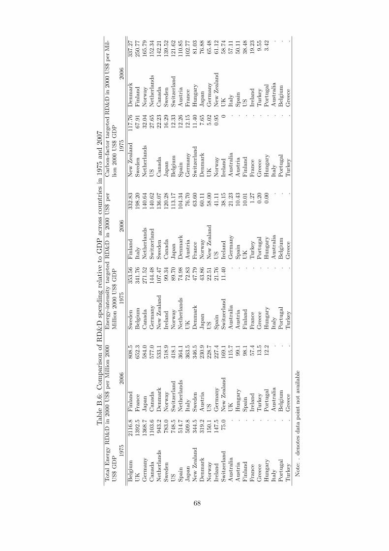
Tab
leB
.6:
Com
par
ison
of
RD
&D
spen
din
gre
lati
veto
GD
Pac
ross
cou
ntr
ies
in197
5an
d20
07T
ota
lE
ner
gy
RD
&D
in2000
US$
per
Million
2000
US$
GD
PE
ner
gy-i
nte
nsi
tyta
rget
edR
D&
Din
2000
US$
per
Million
2000
US$
GD
PC
arb
on-f
act
or
targ
eted
RD
&D
in2000
US$
per
Mil-
lion
2000
US$
GD
P1975
2006
1975
2006
1975
2006
Bel
giu
m2116.8
Fin
land
808.5
Sw
eden
353.5
6F
inla
nd
332.8
3N
ewZ
eala
nd
117.7
6D
enm
ark
337.2
7U
K1392.5
Fra
nce
652.3
Bel
giu
m341.7
6It
aly
198.2
0Sw
eden
67.9
1F
inla
nd
250.7
7G
erm
any
1368.7
Japan
584.0
Canada
271.5
2N
ether
lands
140.6
4N
ether
lands
32.0
4N
orw
ay165.7
9C
anada
1103.6
Canada
577.0
Ger
many
144.4
8Sw
itze
rland
140.6
2U
S27.6
5N
ether
lands
152.3
4N
ether
lands
943.2
Den
mark
533.1
New
Zea
land
107.4
7Sw
eden
136.0
7C
anada
22.2
3C
anada
142.2
1Sw
eden
783.0
Norw
ay518.9
Irel
and
99.3
4C
anada
120.2
8Japan
16.2
9Sw
eden
139.5
2U
S748.5
Sw
itze
rland
418.1
Norw
ay89.7
0Japan
113.1
7B
elgiu
m12.3
3Sw
itze
rland
121.6
2Spain
514.7
Net
her
lands
364.1
Net
her
lands
74.9
8D
enm
ark
104.3
4Spain
12.2
6A
ust
ria
110.8
5Japan
509.8
Italy
363.5
UK
72.8
3A
ust
ria
76.7
0G
erm
any
12.1
5F
rance
102.7
7N
ewZ
eala
nd
344.5
Sw
eden
346.5
Den
mark
47.7
9F
rance
63.6
0Sw
itze
rland
11.4
0H
ungary
81.0
3D
enm
ark
319.2
Aust
ria
230.9
Japan
43.8
6N
orw
ay60.1
1D
enm
ark
7.6
5Japan
76.8
8N
orw
ay150.1
US
228.7
US
22.5
1N
ewZ
eala
nd
58.0
0U
K5.0
2G
erm
any
65.4
8Ir
eland
147.5
Ger
many
227.4
Spain
21.7
6U
S41.1
1N
orw
ay0.9
5N
ewZ
eala
nd
61.1
2Sw
itze
rland
75.0
New
Zea
land
169.1
Sw
itze
rland
11.4
0Ir
eland
38.1
5Ir
eland
0U
K58.7
4A
ust
ralia
.U
K115.7
Aust
ralia
.G
erm
any
21.2
3A
ust
ralia
.It
aly
57.1
1A
ust
ria
.H
ungary
99.1
Aust
ria
.Spain
10.4
3A
ust
ria
.Spain
50.1
1F
inla
nd
.Spain
98.1
Fin
land
.U
K10.0
1F
inla
nd
.U
S38.4
8F
rance
.Ir
eland
57.4
Fra
nce
.T
urk
ey1.2
7F
rance
.Ir
eland
19.2
3G
reec
e.
Turk
ey13.5
Gre
ece
.P
ort
ugal
0.2
0G
reec
e.
Turk
ey9.5
5H
ungary
.P
ort
ugal
12.2
Hungary
.H
ungary
0.0
0H
ungary
.P
ort
ugal
3.4
2It
aly
.A
ust
ralia
.It
aly
.A
ust
ralia
.It
aly
.A
ust
ralia
.P
ort
ugal
.B
elgiu
m.
Port
ugal
.B
elgiu
m.
Port
ugal
.B
elgiu
m.
Turk
ey.
Gre
ece
.T
urk
ey.
Gre
ece
.T
urk
ey.
Gre
ece
.
Note
:.
den
ote
sdata
poin
tnot
available
68
Table B.7: Classification of IEA (2008) public energy R&D expenditure data
Energy
use
Carbon
intensity
GROUP 1: ENERGY EFFICIENCY X
I.1 Industry
I.2 Residential Commercial
I.3 Transportation
I.4 Other Conservation
GROUP II: FOSSIL FUELS
II.1 Total Oil and Gas
II.1.1 Enhanced oil and gas production
II.1.2 Refining transport and storage of oil and gas X
II.1.3 Non-conventional oil and gas production
II.1.4 Oil and gas combustion X
II.1.5 Oil and gas conversion
II.1.6 Other oil and gas
II.2 Total Coal
II.2.1 Coal production and preparation and transport X
II.2.2 Coal combustion X
II.2.3 Coal conversion (excluding IGCC)
II.2.4 Other coal
II.3 Total CO2 Capture and Storage X
II.3.1 CO2 capture/separation
II.3.2 CO2 transport
II.3.3 CO2 storage
GROUP III: RENEWABLE ENERGY SOURCES X
III.1 Total Solar Energy
III.1.1 Solar heating and cooling (including day lighting)
III.1.2 Photovoltaics
III.1.3 Solar thermal-power and high-temperature applications
III.2 Wind Energy
III.3 Ocean Energy
III.4 Total Bio-Energy
III.4.1 Production of transport biofuels including from wastes
III.4.2 Production of other biomass-derived fuels including from wastes
III.4.3 Applications for heat and electricity
III.4.4 Other bio-energy
III.5 Geothermal Energy
III.6 Total Hydropower
III.6.1 Large hydropower (capacity >10 MW)
III.6.2 Small hydropower (capacity <10 MW)
III.7 Other Renewables
69
GROUP IV: NUCLEAR FISSION and FUSION
IV.1 Total Nuclear Fission
IV.1.1 Light-water reactors (LWRs)
IV.1.2 Other converter reactors
IV.1.3 Fuel cycle
IV.1.4 Nuclear supporting technology
IV.1.5 Nuclear breeder
IV.1.6 Other nuclear fission
IV.2 Nuclear Fusion
GROUP V: HYDROGEN AND FUEL CELLS X
V.1 Total Hydrogen
V.1.1 Hydrogen production
V.1.2 Hydrogen storage
V.1.3 Hydrogen transport and distribution
V.1.4 Other infrastructure and systems R&D
V.1.5 Hydrogen end uses including combustion; excluding fuel cells
V.2 Total Fuel Cells
V.2.1 Stationary applications
V.2.2 Mobile applications
V.2.3 Other applications
GROUP VI: OTHER POWER AND STORAGE TECHS X
VI.1 Electric Power Conversion
VI.2 Electricity Transmission and Distribution
VI.3 Energy Storage
GROUP VII: TOTAL OTHER TECHNOLOGIES OR RESEARCH
VII.1 Energy System Analysis
VII.2 Other
TOTAL ENERGY RD&D
The public energy R&D expenditure categories have been classified into 1) energy use and 2)
carbon intensity targeted spending for the purpose of this study. The choices of categories
mostly follow the classification in Garrone and Grilli (2010, p.5611), with the most important
difference being that I classify all spending on renewable energies as targeted at the carbon
intensity, given this is generally the most important stated rationale for these expenditures,
whereas Garrone and Grilli classified some of the sub-categories as targeted at energy use.
Furthermore, unlike Garrone and Grilli I do not classify nuclear power as carbon intensity
targeted spending; while being a low-carbon energy source by itself, the use of nuclear power
is not considered to be a viable component of a low-carbon energy system given that its lack
of flexible deployment represents a hindrance to the increased use of renewables.
70

C Additional regression results for Chapter 4
71
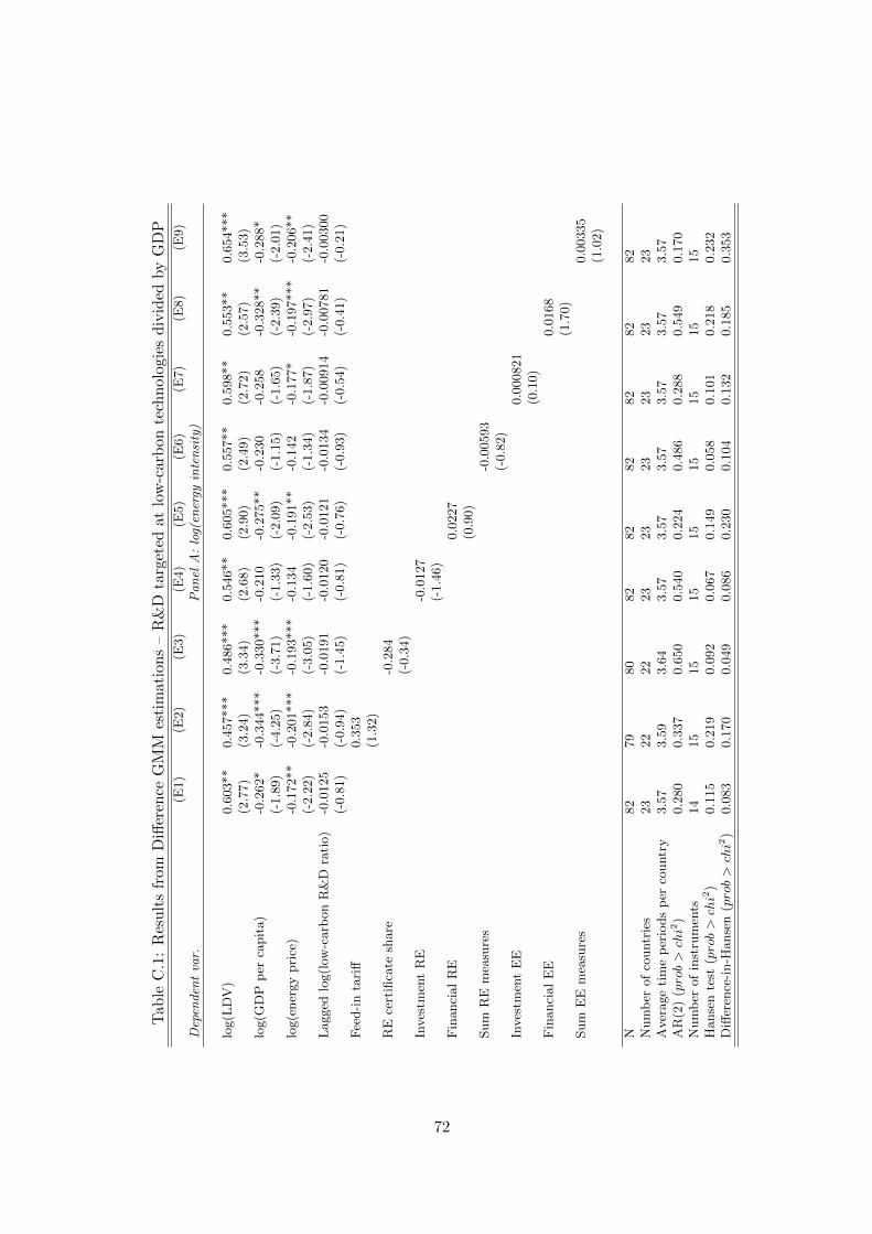
Tab
leC
.1:
Res
ult
sfr
om
Diff
eren
ceG
MM
esti
mat
ion
s–
R&
Dta
rget
edat
low
-car
bon
tech
nolo
gie
sd
ivid
edby
GD
P(E
1)
(E2)
(E3)
(E4)
(E5)
(E6)
(E7)
(E8)
(E9)
Dep
end
ent
var.
Pa
nel
A:
log(
ener
gyin
ten
sity
)
log(L
DV
)0.6
03**
0.4
57***
0.4
86***
0.5
46**
0.6
05***
0.5
57**
0.5
98**
0.5
53**
0.6
54***
(2.7
7)
(3.2
4)
(3.3
4)
(2.6
8)
(2.9
0)
(2.4
9)
(2.7
2)
(2.5
7)
(3.5
3)
log(G
DP
per
capit
a)
-0.2
62*
-0.3
44***
-0.3
30***
-0.2
10
-0.2
75**
-0.2
30
-0.2
58
-0.3
28**
-0.2
88*
(-1.8
9)
(-4.2
5)
(-3.7
1)
(-1.3
3)
(-2.0
9)
(-1.1
5)
(-1.6
5)
(-2.3
9)
(-2.0
1)
log(e
ner
gy
pri
ce)
-0.1
72**
-0.2
01***
-0.1
93***
-0.1
34
-0.1
91**
-0.1
42
-0.1
77*
-0.1
97***
-0.2
06**
(-2.2
2)
(-2.8
4)
(-3.0
5)
(-1.6
0)
(-2.5
3)
(-1.3
4)
(-1.8
7)
(-2.9
7)
(-2.4
1)
Lagged
log(l
ow-c
arb
on
R&
Dra
tio)
-0.0
125
-0.0
153
-0.0
191
-0.0
120
-0.0
121
-0.0
134
-0.0
0914
-0.0
0781
-0.0
0300
(-0.8
1)
(-0.9
4)
(-1.4
5)
(-0.8
1)
(-0.7
6)
(-0.9
3)
(-0.5
4)
(-0.4
1)
(-0.2
1)
Fee
d-i
nta
riff
0.3
53
(1.3
2)
RE
cert
ifica
tesh
are
-0.2
84
(-0.3
4)
Inves
tmen
tR
E-0
.0127
(-1.4
6)
Fin
anci
al
RE
0.0
227
(0.9
0)
Sum
RE
mea
sure
s-0
.00593
(-0.8
2)
Inves
tmen
tE
E0.0
00821
(0.1
0)
Fin
anci
al
EE
0.0
168
(1.7
0)
Sum
EE
mea
sure
s0.0
0335
(1.0
2)
N82
79
80
82
82
82
82
82
82
Num
ber
of
countr
ies
23
22
22
23
23
23
23
23
23
Aver
age
tim
ep
erio
ds
per
countr
y3.5
73.5
93.6
43.5
73.5
73.5
73.5
73.5
73.5
7A
R(2
)(prob>chi2
)0.2
80
0.3
37
0.6
50
0.5
40
0.2
24
0.4
86
0.2
88
0.5
49
0.1
70
Num
ber
of
inst
rum
ents
14
15
15
15
15
15
15
15
15
Hanse
nte
st(prob>chi2
)0.1
15
0.2
19
0.0
92
0.0
67
0.1
49
0.0
58
0.1
01
0.2
18
0.2
32
Diff
eren
ce-i
n-H
anse
n(prob>chi2
)0.0
83
0.1
70
0.0
49
0.0
86
0.2
30
0.1
04
0.1
32
0.1
85
0.3
53
72
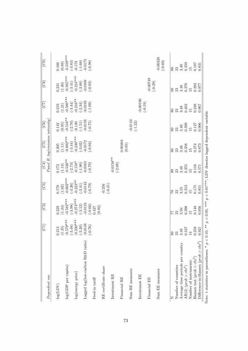
(C1)
(C2)
(C3)
(C4)
(C5)
(C6)
(C7)
(C8)
(C9)
Dep
end
ent
var.
Pa
nel
B:
log(
emis
sio
nin
ten
sity
)
log(L
DV
)0.2
13
0.2
29
0.1
70
0.1
73
0.2
05
0.1
42
0.2
19
0.2
31
0.1
66
(1.3
5)
(1.3
4)
(1.0
2)
(1.1
3)
(1.1
1)
(0.9
5)
(1.2
1)
(1.4
0)
(0.8
9)
log(G
DP
per
capit
a)
-0.5
79***
-0.5
82***
-0.6
02***
-0.5
26**
-0.6
02***
-0.5
16**
-0.5
80***
-0.5
65***
-0.5
59***
(-3.4
8)
(-3.9
8)
(-3.2
6)
(-2.7
3)
(-3.4
4)
(-2.7
0)
(-3.4
4)
(-3.4
1)
(-3.8
3)
log(e
ner
gy
pri
ce)
-0.2
30***
-0.2
74***
-0.2
23**
-0.1
58*
-0.2
36***
-0.1
40
-0.2
16**
-0.2
24***
-0.1
78
(-3.2
0)
(-3.1
2)
(-2.4
1)
(-1.9
0)
(-3.0
2)
(-1.5
1)
(-2.3
4)
(-3.0
0)
(-1.6
8)
Lagged
log(l
ow-c
arb
on
R&
Dra
tio)
-0.0
148
-0.0
124
-0.0
142
-0.0
165
-0.0
172
-0.0
158
-0.0
193
-0.0
168
-0.0
175
(-0.7
6)
(-0.6
6)
(-0.7
9)
(-0.7
9)
(-0.9
4)
(-0.7
5)
(-1.0
9)
(-0.9
3)
(-0.9
8)
Fee
d-i
nta
riff
0.4
27
(0.9
2)
RE
cert
ifica
tesh
are
-0.2
56
(-0.2
1)
Inves
tmen
tR
E-0
.0158**
(-2.0
8)
Fin
anci
al
RE
0.0
0404
(0.0
5)
Sum
RE
mea
sure
s-0
.0110
(-1.2
2)
Inves
tmen
tE
E-0
.00190
(-0.1
9)
Fin
anci
al
EE
-0.0
0749
(-0.2
9)
Sum
EE
mea
sure
s-0
.00328
(-0.6
9)
N80
77
78
80
80
80
80
80
80
Num
ber
of
countr
ies
23
22
22
23
23
23
23
23
23
Aver
age
tim
ep
erio
ds
per
countr
y3.4
83.5
03.5
53.4
83.4
83.4
83.4
83.4
83.4
8A
R(2
)(prob>chi2
)0.3
47
0.3
98
0.3
13
0.3
55
0.3
58
0.3
99
0.4
02
0.3
76
0.3
59
Num
ber
of
inst
rum
ents
14
15
15
15
15
15
15
15
15
Hanse
nte
st(prob>chi2
)0.2
58
0.1
48
0.1
75
0.1
16
0.2
74
0.1
27
0.2
38
0.2
82
0.1
87
Diff
eren
ce-i
n-H
anse
n(prob>chi2
)0.9
21
0.9
56
0.8
51
0.5
71
0.8
73
0.9
06
0.9
67
0.9
77
0.8
31
Note
:t
stati
stic
sin
pare
nth
eses
;*p<
0.1
0,
**p<
0.0
5,
***p<
0.0
1***;
LD
Vden
ote
sla
gged
dep
enden
tva
riable
73
Tab
leC
.2:
Res
ult
sfr
om
GM
Mes
tim
atio
ns
focu
sin
gon
volu
nta
ryen
ergy
an
dcl
imate
mea
sure
s(E
1)
(E2)
(E3)
(E4)
(E5)
(E6)
(E7)
(E8)
(E9)
(E10)
(E11)
(E12)
Dep
end
ent
var.
Pa
nel
A:
log(
ener
gyin
ten
sity
)
log(L
DV
)0.5
16***
0.5
25***
0.6
03**
0.4
34***
0.4
77***
0.5
18***
0.4
82***
0.5
21***
0.5
09***
0.5
71***
0.6
22***
0.6
21**
(4.2
1)
(4.2
5)
(2.7
7)
(3.2
5)
(2.9
0)
(4.3
6)
(3.7
0)
(2.8
9)
(4.3
5)
(2.9
4)
(3.0
9)
(2.7
9)
log(G
DP
per
cap
ita)
-0.2
86***
-0.2
62***
-0.2
62*
-0.2
99***
-0.2
90***
-0.2
93***
-0.2
74***
-0.2
61***
-0.2
76***
-0.2
66**
-0.2
68*
-0.2
63*
(-3.2
2)
(-4.0
7)
(-1.8
9)
(-3.7
0)
(-3.2
8)
(-3.7
4)
(-4.5
4)
(-4.2
7)
(-3.9
8)
(-2.0
9)
(-1.9
5)
(-1.7
4)
log(e
ner
gy
pri
ce)
-0.1
62**
-0.1
53**
-0.1
72**
-0.1
66***
-0.1
57**
-0.1
70***
-0.1
58***
-0.1
53**
-0.1
65***
-0.1
69*
-0.1
80**
-0.1
82**
(-2.8
1)
(-2.7
8)
(-2.2
2)
(-2.9
5)
(-2.6
1)
(-2.9
8)
(-2.9
4)
(-2.6
6)
(-2.8
6)
(-2.0
4)
(-2.1
8)
(-2.1
3)
Lagged
log(e
ner
gy
R&
Dra
tio)
-0.0
213
-0.0
281**
-0.0
243*
-0.0
213*
(-1.7
0)
(-2.1
0)
(-1.7
3)
(-2.0
2)
Lagged
log(e
ner
gy-e
ffici
ency
R&
Dra
tio)
-0.0
157*
-0.0
197*
-0.0
153
-0.0
161**
(-1.9
1)
(-2.0
1)
(-1.6
4)
(-2.3
2)
Lagged
log(l
ow
-carb
on
R&
Dra
tio)
-0.0
125
-0.0
143
-0.0
111
-0.0
109
(-0.8
1)
(-0.9
2)
(-0.8
9)
(-0.6
8)
Volu
nta
ryR
E-0
.0334
-0.0
279
-0.0
137
(-0.9
1)
(-0.6
0)
(-0.2
7)
Volu
nta
ryE
E-0
.00359
-0.0
00199
0.0
0344
(-0.3
8)
(-0.0
2)
(0.4
0)
Volu
nta
ryC
C0.0
0851
0.0
0560
0.0
149
(0.4
8)
(0.3
0)
(0.8
2)
N82
82
82
82
82
82
82
82
82
82
82
82
Nu
mb
erof
cou
ntr
ies
22
22
23
22
22
22
22
22
22
23
23
23
Aver
age
tim
ep
erio
ds
per
cou
ntr
y3.7
33.7
33.5
73.7
33.7
33.7
33.7
33.7
33.7
33.5
73.5
73.5
7A
R(2
)(prob>
chi2
)0.1
92
0.1
01
0.2
80
0.6
90
0.3
52
0.2
32
0.2
61
0.1
55
0.1
53
0.2
80
0.2
62
0.3
07
Nu
mb
erof
inst
rum
ents
14
14
14
15
15
15
15
15
15
15
15
15
Han
sen
test
(prob>
chi2
)0.2
58
0.3
22
0.1
15
0.2
60
0.2
59
0.2
71
0.2
92
0.3
23
0.3
27
0.1
12
0.1
29
0.1
12
Diff
eren
ce-i
n-H
an
sen
(prob>
chi2
)0.1
92
0.4
72
0.0
83
0.2
19
0.2
90
0.3
67
0.4
65
0.3
38
0.5
10
0.1
45
0.2
04
0.1
78
74
(C1)
(C2)
(C3)
(C4)
(C5)
(C6)
(C7)
(C8)
(C9)
(C10)
(C11)
(C12)
Dep
end
ent
var.
Pa
nel
B:
log(
emis
sio
nin
ten
sity
)
log(L
DV
)0.1
66
0.1
98
0.2
13
0.1
69
0.1
43
0.1
68
0.1
79
0.1
71
0.2
00
0.1
93
0.2
10
0.2
23
(1.6
1)
(1.3
4)
(1.3
5)
(1.5
3)
(1.0
4)
(0.8
7)
(1.1
7)
(1.1
9)
(1.0
9)
(1.5
5)
(1.3
9)
(1.2
3)
log(G
DP
per
cap
ita)
-0.5
86***
-0.5
53***
-0.5
79***
-0.5
45***
-0.5
42***
-0.5
43***
-0.5
05***
-0.5
21***
-0.5
27***
-0.5
61***
-0.5
64***
-0.5
53***
(-4.1
1)
(-3.8
8)
(-3.4
8)
(-4.1
2)
(-3.4
5)
(-3.8
2)
(-3.1
7)
(-2.9
9)
(-3.8
1)
(-3.6
5)
(-3.2
3)
(-3.1
4)
log(e
ner
gy
pri
ce)
-0.2
47***
-0.2
26***
-0.2
30***
-0.2
24**
-0.1
90**
-0.2
13**
-0.2
02***
-0.1
78**
-0.2
09**
-0.2
29***
-0.1
89**
-0.2
19**
(-3.0
7)
(-3.9
7)
(-3.2
0)
(-2.6
8)
(-2.4
5)
(-2.3
9)
(-2.8
9)
(-2.3
1)
(-2.4
7)
(-2.8
4)
(-2.7
3)
(-2.6
8)
Lagged
log(e
ner
gy
R&
Dra
tio)
-0.0
128
-0.0
242
-0.0
267
-0.0
186
(-0.4
1)
(-0.7
3)
(-0.8
1)
(-0.6
6)
Lagged
log(e
ner
gy-e
ffici
ency
R&
Dra
tio)
-0.0
141
-0.0
236
-0.0
280
-0.0
238
(-0.5
9)
(-0.9
4)
(-0.9
7)
(-1.0
2)
Lagged
log(l
ow
-carb
on
R&
Dra
tio)
-0.0
148
-0.0
171
-0.0
167
-0.0
174
(-0.7
6)
(-0.7
7)
(-0.9
2)
(-0.9
9)
Volu
nta
ryR
E-0
.0922
-0.0
973
-0.0
641
(-1.1
4)
(-0.9
9)
(-0.6
7)
Volu
nta
ryE
E-0
.0250
-0.0
171
-0.0
0875
(-1.0
0)
(-0.8
4)
(-0.5
1)
Volu
nta
ryC
C-0
.0405
-0.0
388
-0.0
250
(-1.1
7)
(-1.2
0)
(-0.8
9)
N80
80
80
80
80
80
80
80
80
80
80
80
Nu
mb
erof
cou
ntr
ies
22
22
23
22
22
22
22
22
22
23
23
23
Aver
age
tim
ep
erio
ds
per
cou
ntr
y3.6
43.6
43.4
83.6
43.6
43.6
43.6
43.6
43.6
43.4
83.4
83.4
8A
R(2
)(prob>
chi2
)0.2
83
0.3
22
0.3
47
0.3
51
0.3
25
0.3
34
0.3
26
0.3
62
0.3
78
0.3
60
0.3
70
0.4
06
Nu
mb
erof
inst
rum
ents
14
14
14
15
15
15
15
15
15
15
15
15
Han
sen
test
(prob>
chi2
)0.2
08
0.2
19
0.2
58
0.2
11
0.1
52
0.2
01
0.2
16
0.2
80
0.2
69
0.1
90
0.2
38
0.2
98
Diff
eren
ce-i
n-H
an
sen
(prob>
chi2
)0.6
78
0.8
10
0.9
21
0.9
68
0.8
50
0.7
76
0.9
34
0.9
35
0.8
03
0.8
64
0.9
55
0.9
46
Note
:t
stati
stic
sin
pare
nth
eses
;*p<
0.1
0,
**p<
0.0
5,
***p<
0.0
1***;
LD
Vd
enote
sla
gged
dep
end
ent
vari
ab
le
75
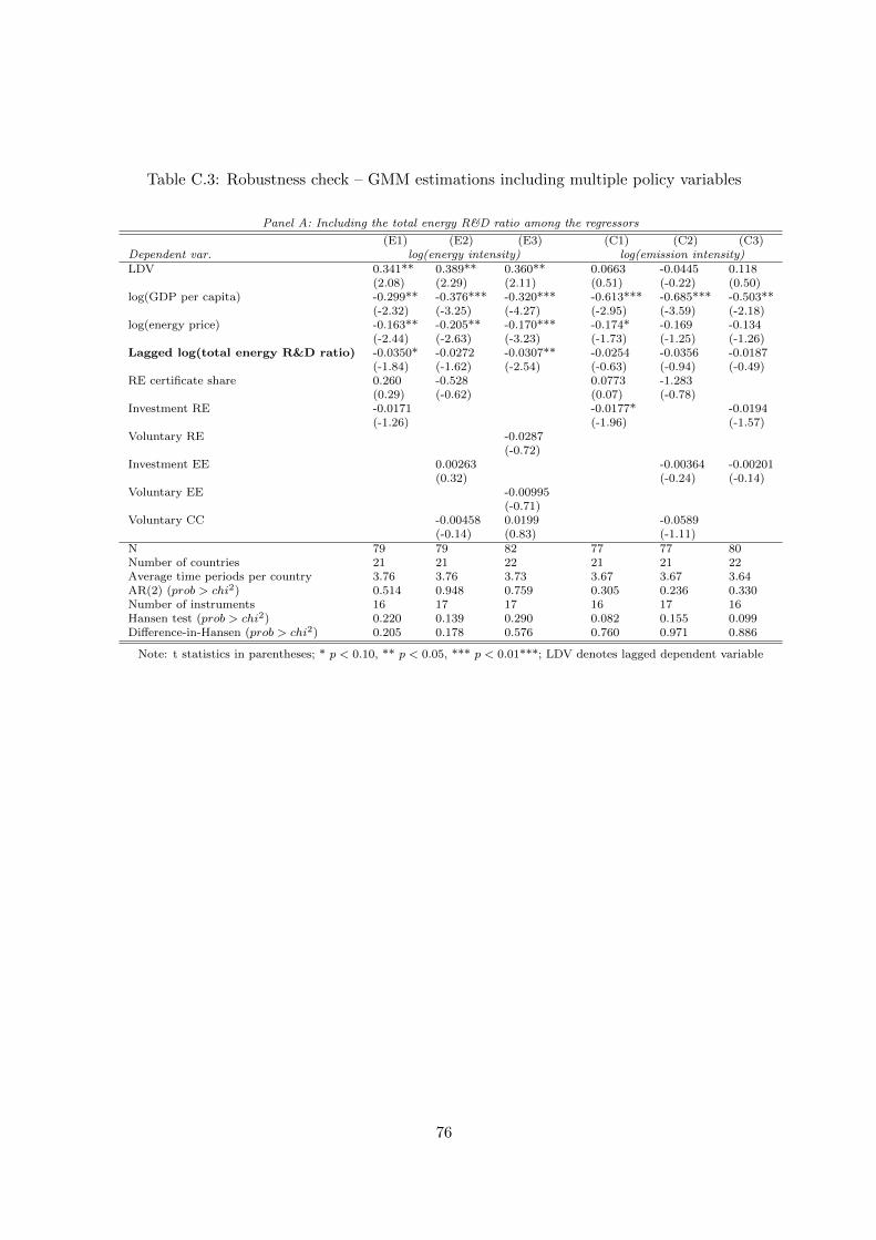
Table C.3: Robustness check – GMM estimations including multiple policy variables
Panel A: Including the total energy R&D ratio among the regressors
(E1) (E2) (E3) (C1) (C2) (C3)Dependent var. log(energy intensity) log(emission intensity)LDV 0.341** 0.389** 0.360** 0.0663 -0.0445 0.118
(2.08) (2.29) (2.11) (0.51) (-0.22) (0.50)log(GDP per capita) -0.299** -0.376*** -0.320*** -0.613*** -0.685*** -0.503**
(-2.32) (-3.25) (-4.27) (-2.95) (-3.59) (-2.18)log(energy price) -0.163** -0.205** -0.170*** -0.174* -0.169 -0.134
(-2.44) (-2.63) (-3.23) (-1.73) (-1.25) (-1.26)Lagged log(total energy R&D ratio) -0.0350* -0.0272 -0.0307** -0.0254 -0.0356 -0.0187
(-1.84) (-1.62) (-2.54) (-0.63) (-0.94) (-0.49)RE certificate share 0.260 -0.528 0.0773 -1.283
(0.29) (-0.62) (0.07) (-0.78)Investment RE -0.0171 -0.0177* -0.0194
(-1.26) (-1.96) (-1.57)Voluntary RE -0.0287
(-0.72)Investment EE 0.00263 -0.00364 -0.00201
(0.32) (-0.24) (-0.14)Voluntary EE -0.00995
(-0.71)Voluntary CC -0.00458 0.0199 -0.0589
(-0.14) (0.83) (-1.11)N 79 79 82 77 77 80Number of countries 21 21 22 21 21 22Average time periods per country 3.76 3.76 3.73 3.67 3.67 3.64AR(2) (prob > chi2) 0.514 0.948 0.759 0.305 0.236 0.330Number of instruments 16 17 17 16 17 16Hansen test (prob > chi2) 0.220 0.139 0.290 0.082 0.155 0.099Difference-in-Hansen (prob > chi2) 0.205 0.178 0.576 0.760 0.971 0.886
Note: t statistics in parentheses; * p < 0.10, ** p < 0.05, *** p < 0.01***; LDV denotes lagged dependent variable
76
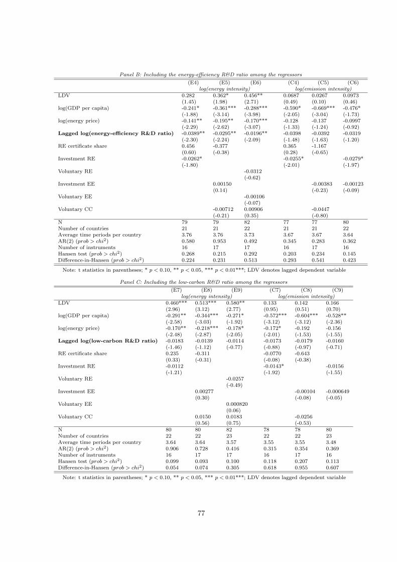
Panel B: Including the energy-efficiency R&D ratio among the regressors
(E4) (E5) (E6) (C4) (C5) (C6)log(energy intensity) log(emission intensity)
LDV 0.282 0.362* 0.456** 0.0687 0.0267 0.0973(1.45) (1.98) (2.71) (0.49) (0.10) (0.46)
log(GDP per capita) -0.241* -0.361*** -0.288*** -0.590* -0.669*** -0.476*(-1.88) (-3.14) (-3.98) (-2.05) (-3.04) (-1.73)
log(energy price) -0.141** -0.195** -0.170*** -0.128 -0.137 -0.0997(-2.29) (-2.62) (-3.07) (-1.33) (-1.24) (-0.92)
Lagged log(energy-efficiency R&D ratio) -0.0389** -0.0295** -0.0196** -0.0398 -0.0392 -0.0319(-2.30) (-2.24) (-2.09) (-1.48) (-1.63) (-1.20)
RE certificate share 0.456 -0.377 0.365 -1.167(0.60) (-0.38) (0.28) (-0.65)
Investment RE -0.0262* -0.0255* -0.0279*(-1.80) (-2.01) (-1.97)
Voluntary RE -0.0312(-0.62)
Investment EE 0.00150 -0.00383 -0.00123(0.14) (-0.23) (-0.09)
Voluntary EE -0.00106(-0.07)
Voluntary CC -0.00712 0.00906 -0.0447(-0.21) (0.35) (-0.80)
N 79 79 82 77 77 80Number of countries 21 21 22 21 21 22Average time periods per country 3.76 3.76 3.73 3.67 3.67 3.64AR(2) (prob > chi2) 0.580 0.953 0.492 0.345 0.283 0.362Number of instruments 16 17 17 16 17 16Hansen test (prob > chi2) 0.268 0.215 0.292 0.203 0.234 0.145Difference-in-Hansen (prob > chi2) 0.224 0.231 0.513 0.293 0.541 0.423
Note: t statistics in parentheses; * p < 0.10, ** p < 0.05, *** p < 0.01***; LDV denotes lagged dependent variable
Panel C: Including the low-carbon R&D ratio among the regressors
(E7) (E8) (E9) (C7) (C8) (C9)log(energy intensity) log(emission intensity)
LDV 0.460*** 0.513*** 0.580** 0.133 0.142 0.166(2.96) (3.12) (2.77) (0.95) (0.51) (0.70)
log(GDP per capita) -0.291** -0.344*** -0.271* -0.572*** -0.604*** -0.528**(-2.58) (-3.03) (-1.92) (-3.12) (-3.12) (-2.36)
log(energy price) -0.170** -0.218*** -0.178* -0.172* -0.192 -0.156(-2.48) (-2.87) (-2.05) (-2.01) (-1.53) (-1.55)
Lagged log(low-carbon R&D ratio) -0.0183 -0.0139 -0.0114 -0.0173 -0.0179 -0.0160(-1.46) (-1.12) (-0.77) (-0.88) (-0.97) (-0.71)
RE certificate share 0.235 -0.311 -0.0770 -0.643(0.33) (-0.31) (-0.08) (-0.38)
Investment RE -0.0112 -0.0143* -0.0156(-1.21) (-1.92) (-1.55)
Voluntary RE -0.0257(-0.49)
Investment EE 0.00277 -0.00104 -0.000649(0.30) (-0.08) (-0.05)
Voluntary EE 0.000820(0.06)
Voluntary CC 0.0150 0.0183 -0.0256(0.56) (0.75) (-0.53)
N 80 80 82 78 78 80Number of countries 22 22 23 22 22 23Average time periods per country 3.64 3.64 3.57 3.55 3.55 3.48AR(2) (prob > chi2) 0.906 0.728 0.416 0.315 0.354 0.369Number of instruments 16 17 17 16 17 16Hansen test (prob > chi2) 0.099 0.093 0.100 0.118 0.207 0.113Difference-in-Hansen (prob > chi2) 0.054 0.074 0.305 0.618 0.955 0.607
Note: t statistics in parentheses; * p < 0.10, ** p < 0.05, *** p < 0.01***; LDV denotes lagged dependent variable
77
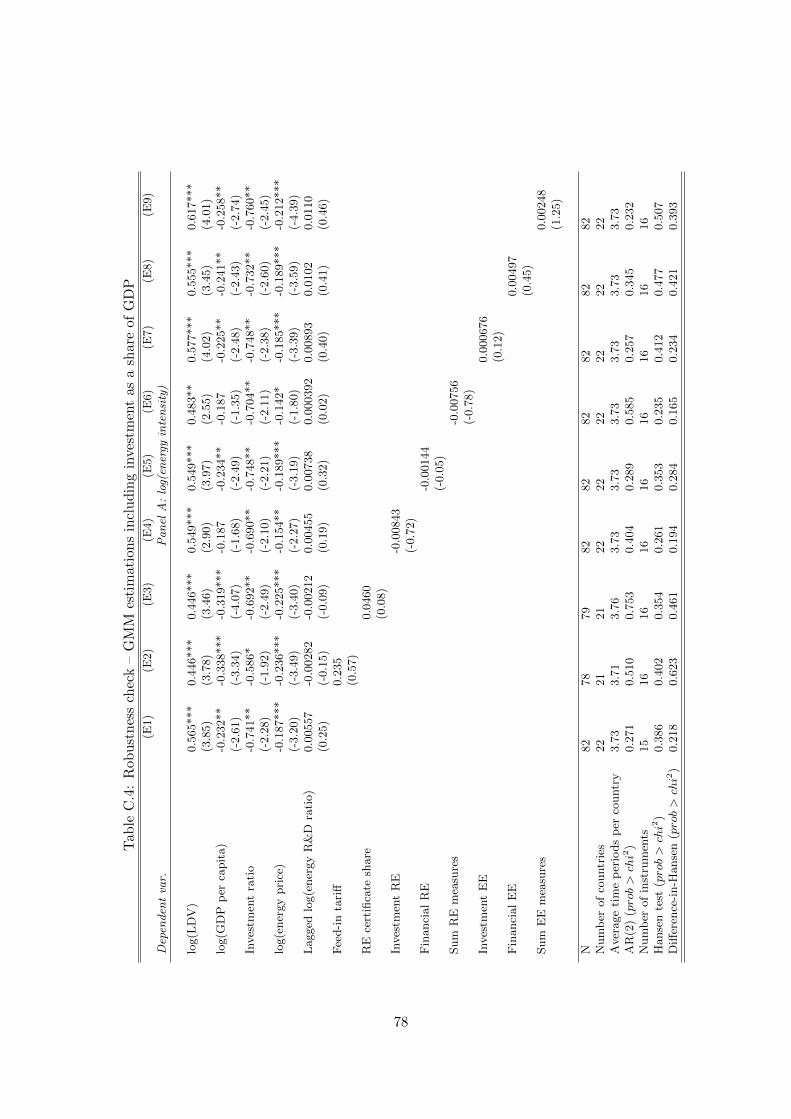
Tab
leC
.4:
Rob
ust
nes
sch
eck
–G
MM
esti
mat
ion
sin
clu
din
gin
vest
men
tas
ash
are
of
GD
P(E
1)
(E2)
(E3)
(E4)
(E5)
(E6)
(E7)
(E8)
(E9)
Dep
end
ent
var.
Pa
nel
A:
log(
ener
gyin
ten
sity
)
log(L
DV
)0.5
65***
0.4
46***
0.4
46***
0.5
49***
0.5
49***
0.4
83**
0.5
77***
0.5
55***
0.6
17***
(3.8
5)
(3.7
8)
(3.4
6)
(2.9
0)
(3.9
7)
(2.5
5)
(4.0
2)
(3.4
5)
(4.0
1)
log(G
DP
per
capit
a)
-0.2
32**
-0.3
38***
-0.3
19***
-0.1
87
-0.2
34**
-0.1
87
-0.2
25**
-0.2
41**
-0.2
58**
(-2.6
1)
(-3.3
4)
(-4.0
7)
(-1.6
8)
(-2.4
9)
(-1.3
5)
(-2.4
8)
(-2.4
3)
(-2.7
4)
Inves
tmen
tra
tio
-0.7
41**
-0.5
86*
-0.6
92**
-0.6
90**
-0.7
48**
-0.7
04**
-0.7
48**
-0.7
32**
-0.7
60**
(-2.2
8)
(-1.9
2)
(-2.4
9)
(-2.1
0)
(-2.2
1)
(-2.1
1)
(-2.3
8)
(-2.6
0)
(-2.4
5)
log(e
ner
gy
pri
ce)
-0.1
87***
-0.2
36***
-0.2
25***
-0.1
54**
-0.1
89***
-0.1
42*
-0.1
85***
-0.1
89***
-0.2
12***
(-3.2
0)
(-3.4
9)
(-3.4
0)
(-2.2
7)
(-3.1
9)
(-1.8
0)
(-3.3
9)
(-3.5
9)
(-4.3
9)
Lagged
log(e
ner
gy
R&
Dra
tio)
0.0
0557
-0.0
0282
-0.0
0212
0.0
0455
0.0
0738
0.0
00392
0.0
0893
0.0
102
0.0
110
(0.2
5)
(-0.1
5)
(-0.0
9)
(0.1
9)
(0.3
2)
(0.0
2)
(0.4
0)
(0.4
1)
(0.4
6)
Fee
d-i
nta
riff
0.2
35
(0.5
7)
RE
cert
ifica
tesh
are
0.0
460
(0.0
8)
Inves
tmen
tR
E-0
.00843
(-0.7
2)
Fin
anci
al
RE
-0.0
0144
(-0.0
5)
Sum
RE
mea
sure
s-0
.00756
(-0.7
8)
Inves
tmen
tE
E0.0
00676
(0.1
2)
Fin
anci
al
EE
0.0
0497
(0.4
5)
Sum
EE
mea
sure
s0.0
0248
(1.2
5)
N82
78
79
82
82
82
82
82
82
Num
ber
of
countr
ies
22
21
21
22
22
22
22
22
22
Aver
age
tim
ep
erio
ds
per
countr
y3.7
33.7
13.7
63.7
33.7
33.7
33.7
33.7
33.7
3A
R(2
)(prob>chi2
)0.2
71
0.5
10
0.7
53
0.4
04
0.2
89
0.5
85
0.2
57
0.3
45
0.2
32
Num
ber
of
inst
rum
ents
15
16
16
16
16
16
16
16
16
Hanse
nte
st(prob>chi2
)0.3
86
0.4
02
0.3
54
0.2
61
0.3
53
0.2
35
0.4
12
0.4
77
0.5
07
Diff
eren
ce-i
n-H
anse
n(prob>chi2
)0.2
18
0.6
23
0.4
61
0.1
94
0.2
84
0.1
65
0.2
34
0.4
21
0.3
93
78
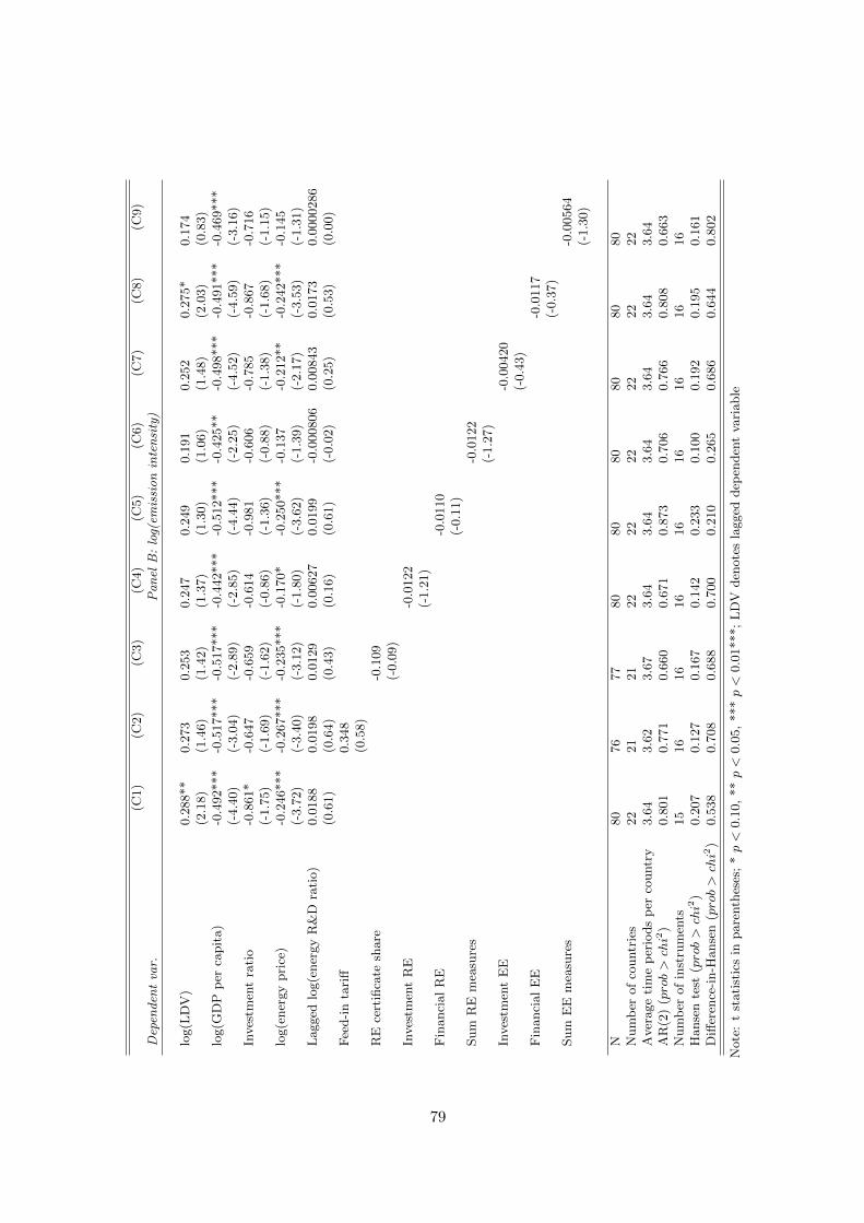
(C1)
(C2)
(C3)
(C4)
(C5)
(C6)
(C7)
(C8)
(C9)
Dep
end
ent
var.
Pa
nel
B:
log(
emis
sio
nin
ten
sity
)
log(L
DV
)0.2
88**
0.2
73
0.2
53
0.2
47
0.2
49
0.1
91
0.2
52
0.2
75*
0.1
74
(2.1
8)
(1.4
6)
(1.4
2)
(1.3
7)
(1.3
0)
(1.0
6)
(1.4
8)
(2.0
3)
(0.8
3)
log(G
DP
per
capit
a)
-0.4
92***
-0.5
17***
-0.5
17***
-0.4
42***
-0.5
12***
-0.4
25**
-0.4
98***
-0.4
91***
-0.4
69***
(-4.4
0)
(-3.0
4)
(-2.8
9)
(-2.8
5)
(-4.4
4)
(-2.2
5)
(-4.5
2)
(-4.5
9)
(-3.1
6)
Inves
tmen
tra
tio
-0.8
61*
-0.6
47
-0.6
59
-0.6
14
-0.9
81
-0.6
06
-0.7
85
-0.8
67
-0.7
16
(-1.7
5)
(-1.6
9)
(-1.6
2)
(-0.8
6)
(-1.3
6)
(-0.8
8)
(-1.3
8)
(-1.6
8)
(-1.1
5)
log(e
ner
gy
pri
ce)
-0.2
46***
-0.2
67***
-0.2
35***
-0.1
70*
-0.2
50***
-0.1
37
-0.2
12**
-0.2
42***
-0.1
45
(-3.7
2)
(-3.4
0)
(-3.1
2)
(-1.8
0)
(-3.6
2)
(-1.3
9)
(-2.1
7)
(-3.5
3)
(-1.3
1)
Lagged
log(e
ner
gy
R&
Dra
tio)
0.0
188
0.0
198
0.0
129
0.0
0627
0.0
199
-0.0
00806
0.0
0843
0.0
173
0.0
000286
(0.6
1)
(0.6
4)
(0.4
3)
(0.1
6)
(0.6
1)
(-0.0
2)
(0.2
5)
(0.5
3)
(0.0
0)
Fee
d-i
nta
riff
0.3
48
(0.5
8)
RE
cert
ifica
tesh
are
-0.1
09
(-0.0
9)
Inves
tmen
tR
E-0
.0122
(-1.2
1)
Fin
anci
al
RE
-0.0
110
(-0.1
1)
Sum
RE
mea
sure
s-0
.0122
(-1.2
7)
Inves
tmen
tE
E-0
.00420
(-0.4
3)
Fin
anci
al
EE
-0.0
117
(-0.3
7)
Sum
EE
mea
sure
s-0
.00564
(-1.3
0)
N80
76
77
80
80
80
80
80
80
Num
ber
of
countr
ies
22
21
21
22
22
22
22
22
22
Aver
age
tim
ep
erio
ds
per
countr
y3.6
43.6
23.6
73.6
43.6
43.6
43.6
43.6
43.6
4A
R(2
)(prob>chi2
)0.8
01
0.7
71
0.6
60
0.6
71
0.8
73
0.7
06
0.7
66
0.8
08
0.6
63
Num
ber
of
inst
rum
ents
15
16
16
16
16
16
16
16
16
Hanse
nte
st(prob>chi2
)0.2
07
0.1
27
0.1
67
0.1
42
0.2
33
0.1
00
0.1
92
0.1
95
0.1
61
Diff
eren
ce-i
n-H
anse
n(prob>chi2
)0.5
38
0.7
08
0.6
88
0.7
00
0.2
10
0.2
65
0.6
86
0.6
44
0.8
02
Note
:t
stati
stic
sin
pare
nth
eses
;*p<
0.1
0,
**p<
0.0
5,
***p<
0.0
1***;
LD
Vden
ote
sla
gged
dep
enden
tva
riable
79

Eidesstattliche Erklarung
Ich erklare hiermit an Eides Statt, dass ich meine Doktorarbeit “Essays on Decarbonising
Energy Supply” selbstandig und ohne fremde Hilfe angefertigt habe und dass ich alle von
anderen Autoren wortlich ubernommenen Stellen, wie auch die sich an die Gedanken anderer
Autoren eng anlehnenden Ausfuhrungen meiner Arbeit, besonders gekennzeichnet und die
Quellen nach den mir angegebenen Richtlinien zitiert habe.
Datum (Bettina Kretschmer)
80
Curriculum vitae
Personal informationName Bettina KretschmerAddress Rue du Chien Marin 20, 1000 BrusselsEmail [email protected] +32-487-383037Date of birth 05.08.1982, Duren
Education10/2007-10/2012 Doctoral programme ‘Quantitative Economics’, CAU Kiel09/2006-08/2007 Master of Science in ‘International Economic Studies’, Universiteit
Maastricht09/2002-08/2005 Bachelor of Arts in ‘European Studies’, Universiteit Maastricht08/1993-06/2002 Abitur, Burgau-Gymnasium Duren
Professional experienceSince 11/2010 Policy analyst at the Institute for European Environmental Policy,
London and Brussels10/2007-10/2010 Research assistant at the Kiel Institute for the World Economy,
research area ‘The Environment and Natural Resources’03/2010-07/2010 Traineeship in the European Commission, DG Energy, Brussels
Selected publicationsKeegan, D., Kretschmer, B., Elbersen, B. and Panoutsou, C. (forthcoming). Cascading Use:A Systematic Approach to Biomass beyond the Energy Sector. Biofuels, Bioproducts andBiorefining.
Kretschmer, B., Hubler, M. and Nunnenkamp, P. (2013). Does Foreign Aid Reduce Energyand Carbon Intensities of Developing Economies? Journal of International Development 25,67-91.
Kretschmer, B. and Peterson, S. (2010). Integrating Bioenergy into Computable GeneralEquilibrium Models A Survey. Energy Economics 32, 673-686.
Kretschmer, B., Narita, D. and Peterson, S. (2009). The economic effects of the EU biofueltarget. Energy Economics 31, S285-S294.
81