Embed Size (px)
Citation preview
Florida International UniversityFIU Digital Commons
FIU Electronic Theses and Dissertations University Graduate School
9-16-2008
Essays on Durable Goods Consumption and FirmInnovationZhao RongFlorida International University, [email protected]
DOI: 10.25148/etd.FI10022546Follow this and additional works at: https://digitalcommons.fiu.edu/etd
This work is brought to you for free and open access by the University Graduate School at FIU Digital Commons. It has been accepted for inclusion inFIU Electronic Theses and Dissertations by an authorized administrator of FIU Digital Commons. For more information, please contact [email protected].
Recommended CitationRong, Zhao, "Essays on Durable Goods Consumption and Firm Innovation" (2008). FIU Electronic Theses and Dissertations. 215.https://digitalcommons.fiu.edu/etd/215
FLORIDA INTERNATIONAL UNIVERSITY
Miami, Florida
ESSAYS ON DURABLE GOODS CONSUMPTION
AND FIRM INNOVATION
A dissertation submitted in partial fulfillment of the
requirements for the degree of
DOCTOR OF PHILOSOPHY
in
ECONOMICS
by
Zhao Rong
2008

ii
To: Dean Kenneth Furton College of Arts and Sciences
This dissertation, written by Zhao Rong, and entitled Essays on Durable Goods Consumption and Firm Innovation, having been approved in respect to style and intellectual content, is referred to you for judgment.
We have read this dissertation and recommend that it be approved.
_______________________________________ Cem Karayalcin
_______________________________________
Prasad Bidarkota
_______________________________________ Hassan Zahedi
_______________________________________
Peter Thompson, Major Professor
Date of Defense: September 16, 2008
The dissertation of Zhao Rong is approved.
_______________________________________ Dean Kenneth Furton
College of Arts and Sciences
_______________________________________ Dean George Walker
University Graduate School
Florida International University, 2008

iii
© Copyright 2008 by Zhao Rong
All rights reserved.

iv
DEDICATION
I dedicate this dissertation to my wife, Ying, without whose love this would never
have been completed; to my parents, whose belief in my abilities never wavered.

v
ACKNOWLEDGMENTS
The dissertation records some of my thoughts over the past three years, and it is just a
beginning of better ideas.
Special thanks to my advisor, Peter Thompson. Without him I would not accomplish
my dissertation. Other individuals inspired me at the Department of Economics are John
Boyd, Cem Karayalcin, Prasad Bidarkota, and Jonathan Hill.
I would also like to thank my family for their support. All my efforts become
meaningful because of them.
vi
ABSTRACT OF THE DISSERTATION
ESSAYS ON DURABLE GOODS CONSUMPTION
AND FIRM INNOVATION
by
Zhao Rong
Florida International University, 2008
Miami, Florida
Professor Peter Thompson, Major Professor
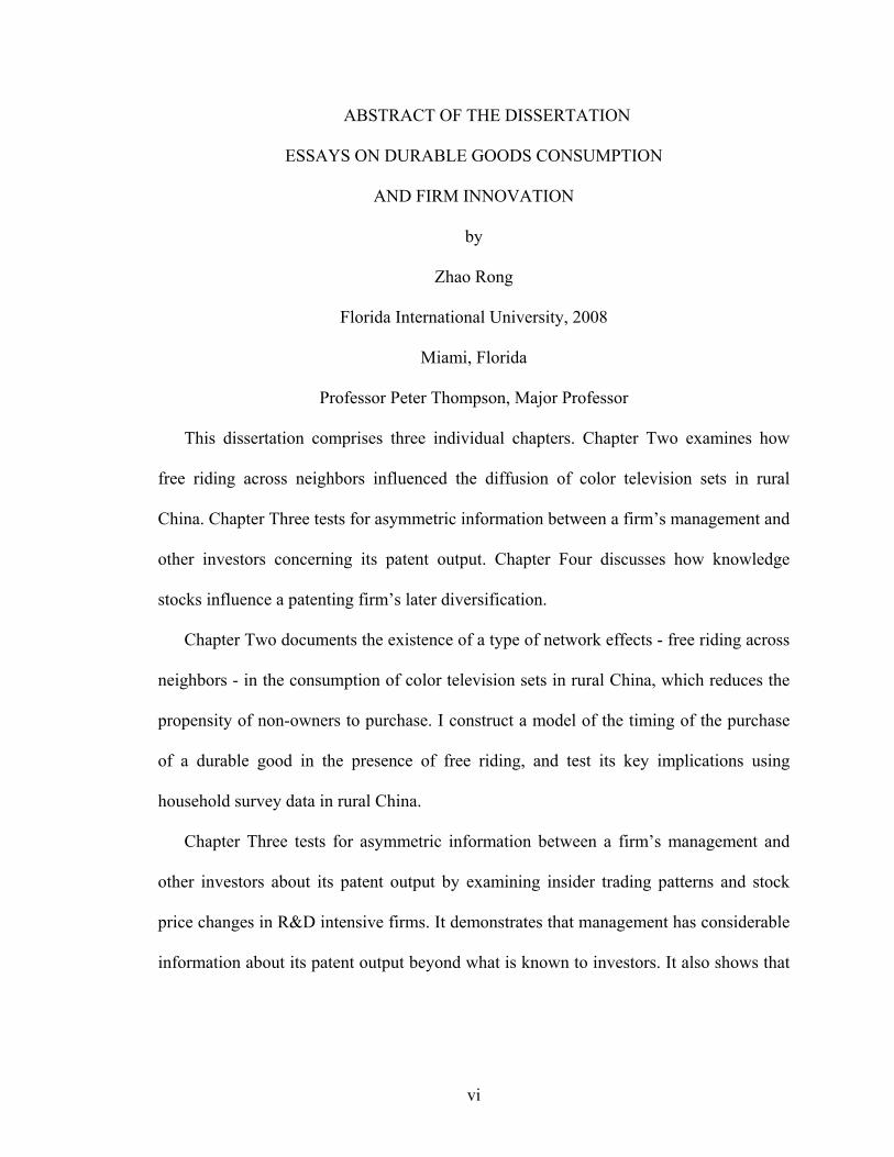
This dissertation comprises three individual chapters. Chapter Two examines how
free riding across neighbors influenced the diffusion of color television sets in rural
China. Chapter Three tests for asymmetric information between a firm’s management and
other investors concerning its patent output. Chapter Four discusses how knowledge
stocks influence a patenting firm’s later diversification.
Chapter Two documents the existence of a type of network effects - free riding across
neighbors - in the consumption of color television sets in rural China, which reduces the
propensity of non-owners to purchase. I construct a model of the timing of the purchase
of a durable good in the presence of free riding, and test its key implications using
household survey data in rural China.
Chapter Three tests for asymmetric information between a firm’s management and
other investors about its patent output by examining insider trading patterns and stock
price changes in R&D intensive firms. It demonstrates that management has considerable
information about its patent output beyond what is known to investors. It also shows that

vii
the predictive power of insider trading patterns on patent output comes from purchases
rather than sales.
Chapter Four discusses two sequential channels through which knowledge stocks may
influence a firm’s later diversification. One is that firms with more knowledge are more
likely to enter a new industry. The other is that firms’ businesses have a better chance of
surviving, conditional on being formed. By examining U.S. public patenting firms in
manufacturing sectors for 1984-1996, I find that knowledge stocks predict the likelihood
of new industry entry when controlling for firm size. However, this predictive power is
weakened when diversification effects are included. On the other hand, a survival study
of newly established segments shows that initial knowledge stocks have significant
positive effects on segment survival, whereas diversification effects are insignificant.

viii
TABLE OF CONTENTS
CHAPTER PAGE
I. INTRODUCTION............................................................................................................1 II. NETWORK EFFECTS AND DURABLE ADOPTION: A TEST USING TELEVISIONS IN RURAL CHINA...................................................................................3
II.1. Introduction ............................................................................................................. 3 II.2. The Model ............................................................................................................... 5 II.3. Data ....................................................................................................................... 10 II.4. Results ................................................................................................................... 12
II.4.1. Initial Ownership Rates.................................................................................. 13 II.4.2. Lagged Ownership Rates ............................................................................... 16 II.4.3. The Distance Effect........................................................................................ 18
II.5. Conclusions ........................................................................................................... 20 References..................................................................................................................... 22 Appendix....................................................................................................................... 23
III. DO INSIDER TRADING PATTERNS PREDICT A FIRM’S PATENT OUTPUT?..........................................................................................................................24
III.1. Introduction.......................................................................................................... 24 III.2. Estimation Settings .............................................................................................. 26 III.3. Data and Variables............................................................................................... 30
III.3.1. Dependent Variable: Patent Output .............................................................. 31 III.3.2. Independent Variable: Insider Trading Patterns ........................................... 36
III.4. Empirical Results ................................................................................................. 39 III.5. Conclusions.......................................................................................................... 51 References..................................................................................................................... 53 Appendix....................................................................................................................... 55
IV. HOW DO KNOWLEDGE STOCKS INFLUENCE THE START-UP AND SURVIVAL OF NEW MANUFACTURING SEGMENTS IN U.S. PATENTING FIRMS?..............................................................................................................................57
IV.1. Introduction......................................................................................................... 57 IV.2. A Simple Model.................................................................................................. 60 IV.3. Data..................................................................................................................... 64
IV.3.1. Dependent Variable: New Industry Entry .................................................. 65 IV.3.2. Independent Variable: Knowledge stocks .................................................. 69
IV.4. Results................................................................................................................. 71 IV.5. Conclusions......................................................................................................... 86 References..................................................................................................................... 88 Appendix....................................................................................................................... 91
VITA..................................................................................................................................98

ix
LIST OF TABLES
TABLE PAGE
Table 2.1. Demographics of 1999 CTV Non-Owners Versus Owners............................. 11
Table 2.2. Probit Estimation of Purchasing CTV Sets since 1997 ................................... 14
Table 2.3. Effects of Initial Ownership Rates on CTV Adoption (Probit) ....................... 15
Table 2.4. Effects of Ownership Rates on Three Durable Goods Adoption..................... 16
Table 2.5. Effects of Lagged Ownership Rates on CTV Adoption (Probit)..................... 18
Table 2.6. Distance Effects on Three Durables Adoption (Probit)................................... 19
Table 3.1. OLS Estimations of CACs on PACs ............................................................... 34
Table 3.2. Transaction Counts for Insider Types.............................................................. 37
Table 3.3. Transaction Counts for Transaction Types...................................................... 38
Table 3.4. Summary Statistics of Firms for 1987-94........................................................ 40
Table 3.5. The First-Stage Estimation using PACs .......................................................... 41
Table 3.6. Explanatory Power of Insider Trading Counts on PACs................................. 43
Table 3.7. The First-Stage Estimation Using CACs ......................................................... 44
Table 3.8. Explanatory Power of Insider Trading Counts on CACs ................................ 45
Table 3.9. Explanatory Power of Insider Trading Counts ................................................ 46
Table 3.10. The First-Stage Estimations by Technological Categories............................ 47
Table 3.11. The Influence of R&D Intensities.................................................................. 49
Table 3.12. Explanatory Power of Insider Trading Value on CACs ................................ 50
Table 4.1. Characteristics in 1984 of Patenting firms and Non-Patenting Firms ............. 66
Table 4.2. Characteristics in 1984 of Patenting firms with Entry VS Those without....... 72
Table 4.3. Probit Estimations of Entry Likelihood on Knowledge Stocks....................... 73
Table 4.4. LP Estimations of Entry Likelihood on Knowledge Stocks ............................ 74
x
Table 4.5. Entry Ratio by Manufacturing Segment Counts in 1984................................. 75
Table 4.6. LP Estimations of Entry Likelihood in all Manufacturing Firms.................... 76
Table 4.7. WLW Estimation of Entry Hazard on Knowledge Stocks .............................. 79
Table 4.8. PH Estimation for Segment Exit Hazard in Patenting Firms........................... 83
Table 4.9. PH Estimation for Segment Exit Hazard in Persistent Patenting Firms .......... 84
Table 4.10. PH Estimation for Segment Exit Hazard in Persistent Manufacturing Firms ......................................................................................................................... 85
Table 4.A1. LP Estimations of Entry Likelihood with Control for Firm Fixed Effects ... 95
Table 4.A2. WLW Estimation of Entry Hazard without Control for Industry Fixed Effects ....................................................................................................................... 96
Table 4.A3. WLW Estimation of Entry Hazard in all Manufacturing Firms ................... 97
xi
LIST OF FIGURES
FIGURE PAGE
Figure 2.1. Solution(s) to the Agent’s Purchasing Problem ............................................... 8
Figure 3.1. Mean Characteristics of the 88 Firms for 1980-99......................................... 33
Figure 3.2. Insider Trading Counts for 1987-99 ............................................................... 39
Figure 4.1. Entry Counts of the 1,101 Firms for 1985-96 ................................................ 67
Figure 4.2. Distributions of Recurrent Entries for 1985-96.............................................. 69
Figure 4.3. Mean Characteristics of Persistent Firms for 1984-96 ................................... 71
Figure 4.4. Kaplan Meier Survival Estimates................................................................... 81

1
I. INTRODUCTION
This dissertation is organized into three main chapters. Chapter II examines how free
riding across neighbors influenced the diffusion of color television sets in rural China.
Chapter III tests for asymmetric information between a firm’s management and other
investors concerning its patent output. Chapter IV discusses how knowledge stocks
influence a patenting firm’s later diversification.
Chapter II documents the existence of a type of network effects - free riding across
neighbors - in the consumption of color television sets in rural China, which reduces the
propensity of non-owners to purchase. I construct a model of the timing of the purchase
of a durable good in the presence of free riding, and test its key implications using
household survey data in rural China.
Chapter III tests for asymmetric information between a firm’s management and other
investors about its patent output by examining insider trading patterns and stock price
changes in R&D intensive firms. It demonstrates that management has considerable
information about its patent output beyond what is known to investors. It also shows that
the predictive power of insider trading patterns on patent output comes from purchases
rather than sales.
Chapter IV discusses two sequential channels through which knowledge stocks may
influence a firm’s later diversification. One is that firms with more knowledge are more
likely to enter a new industry. The other is that firms’ businesses have a better chance of
surviving, conditional on being formed. By examining U.S. public patenting firms in
manufacturing sectors for 1984-1996, I find that knowledge stocks predict the likelihood
of new industry entry when controlling for firm size. However, this predictive power is

2
weakened when diversification effects are included. On the other hand, a survival study
of newly established segments shows that initial knowledge stocks have significant
positive effects on segment survival, whereas diversification effects are insignificant.
3
II. NETWORK EFFECTS AND DURABLE ADOPTION: A TEST USING
TELEVISIONS IN RURAL CHINA
II.1. Introduction
Over a decade ago, Liebowitz and Margolis (1994) noted that "[a]lthough network
effects are pervasive in the economy, we see scant evidence of [their] existence." Since
then, empirical studies establishing the existence of empirically significant network
externalities remain relatively scarce. Moreover, much of this evidence relates to
technology adoption by firms,1 while studies documenting network externalities among
consumers are few and far between. Among the few exceptions, Gandal (1994) shows
that consumers were willing to pay a premium for spreadsheet software compatible with
the Lotus platform and with external database programs; Goolsbee and Klenow (2002)
report that people are more likely to buy their first home computer in areas where a high
fraction of households already own computers; Berndt, Pindyck and Azonlay (2001)
document how network externalities influence the demand for prescription
pharmaceuticals; and Park (2004) finds that network externalities in video cassette
recorders explain much of the dominance of VHS relative to Betamax.
This chapter provides evidence of a type of network effects - the free-riding effect -
among consumers of color television sets (CTVs) in rural China. The intuition is
straightforward, and it reflects a type of consumption externalities that is perhaps peculiar
to developing countries. In rural China, as in other developing countries, the CTV serves
1 For a recent example, see Gowrisankaran and Stavins (2004) on the adoption of electronic transfers, or Bandiera and Rasul (2006) on the adoption of new crops in Mozambique.
4
in part the role of a public good for the neighborhood. When a household purchases a
CTV, neighbors gain because they frequently visit to watch television. The nature of
social interactions within a village induces the host to share use of her television. There is
a network effect involved since the higher the CTV ownership rate the more convenient it
is for a non-owner to free ride. As far as I know, I am the first to document a situation
where a type of network effects deters the purchase of a durable good.
The difficulty in identifying the free-riding effect on CTV adoption comes from the
fact that it is mixed with other effects, here especially network externalities as in
Goolsbee and Klenow (2002), where the larger the size of the network, the more
attractive the durable is to non-owners to purchase. These two effects influence CTV
adoption in the opposite direction and both are generally measured by the local
ownership rate. If one detects a negative gross effect of the ownership rate on the
likelihood of household CTV adoption, he may conclude there is a free-riding effect by
showing that it dominates the effect of network externalities. However, I find that this
gross effect is positive, and thus I fail to detect dominance of the free-riding effect.
In this chapter I test some other implications consistent with the existence of the free-
riding effect. First, in other durable goods such as washing machines and refrigerators,
where there is no free-riding effect, the effect of local ownership rates should be stronger
than CTV. While rural Chinese commonly watch their neighbor’s television, they do not
generally keep food in their refrigerators or use their washing machines. My finding is
consistent with this implication. Second, a proxy to measure the free-riding effect is the
distance between neighbors. As distance raises visiting cost, the free-riding effect would
be weakened, thus having less negative influence on CTV adoption. My regression

5
results show a significantly positive relationship between the likelihood of CTV adoption
and distance when controlling for the local ownership rate. But I fail to detect this in
either washing machine or refrigerator adoption. These conclusions provide evidence of a
free-riding effect in CTV adoption.
The chapter is organized as follows. In Section II.2, I present a dynamic model of a
durable purchase with the presence of free riding and its implications. Section II.3
describes data. Section II.4 reports empirical results. Section II.5 concludes.
II.2. The Model
The model is based on Leahy and Zeira (2005), who discuss the timing and quality
choice of durable goods purchases in a general equilibrium dynamic model. In their
model, both durable and non-durable goods are consumed and the durable good is lumpy.
I ignore general equilibrium considerations and the question of quality choice, while
introducing a free-riding effect.
I consider a village with a continuum of infinitely-lived agents, each of which derives
utility from consumption of a durable and a non-durable good. Agents are identical
except for the utility they receive from consumption of the durable good. The durable
good is homogeneous, does not depreciate, and only a single unit of it can be purchased.
Agents begin life with zero wealth at time t=0, earn income at the rate y, and must pay a
price p for the durable good out of savings.2 Agents discount at the rate ρ, which I
2 The absence of consumption loans and the exogeneity of p are assumptions consistent with the situation in rural China during the period of the survey. In the 1990s, the rural market for CTVs was small relative to urban demand, so consumer prices would reflect primarily urban market conditions.

6
assume equals the interest rate r. Let u(c) denote utility from non-durable good
consumption, and let v denote the flow of utility from durable good consumption. I
assume u(c) is the same for all agents, it is increasing, strictly concave and satisfies
0lim '( )c u c→ = +∞ and lim '( ) 0c u c→∞ = . The flow of utility from consumption of the
durable good is given by
( )
( ),
t v t Tv t
v t T
β γ <⎧⎪= ⎨≥⎪⎩
, (2.1)
where T is the time of the durable purchase, ( )tβ is the local ownership rate, and
[0,1]γ ∈ is a parameter governing the strength of the free-riding effect. Agents differ in
their valuation of v, which for each one is a draw from F(v). Larger value of ( )tβ and γ
increase the utility from consumption of other people’s durable goods and will ceteris
paribus discourage an agent from purchasing her own.
Since I have assumed the interest rate and discount rate are equal, consumption
smoothing implies that non-durable good consumption is constant during the interval
[0, ]T and also during the interval ( , )T ∞ . Thus, under perfect foresight on ( )tβ , the
agent’s problem is
[ ] [ ]1 2
1 2, ,0
max ( ) ( ) ( )T
rt rt
c c TT
e u c t v dt e u c v dtβ γ∞
− −+ + +∫ ∫ , (2.2)
subject to
1 20 0
TrT rt rt rt
T
pe e c dt c e dt ye dt∞ ∞
− − − −+ + ≤∫ ∫ ∫ , (2.3)
10 0
T TrT rt rtpe e c dt ye dt− − −+ ≤∫ ∫ . (2.4)

7
The consumer maximizes her discounted lifetime utility by choosing the amount of
non-durable good consumption at each point in time, and the time of the durable good
purchase, subject to her lifetime budget constraint, (2.3), and her financing constraint,
(2.4).
It is helpful to begin with the situation without externalities, where 0γ = . Local non-
satiation implies that both (2.3) and (2.4) are binding, and that 2c y= .3 It then follows
that 1c y s= − , where
1
rT
rT
rpes
e
−
−=−
(2.5)
is the constant saving rate during [0, ]T . Equation (2.5) enables me to rewrite the agent’s
problem as
( ) ( )
0
1max ( )
1
rT rT rT
rTT
e rpe eU u y u y vr e r
− − −
−≥
− ⎛ ⎞= − + +⎜ ⎟−⎝ ⎠
, (2.6)
with necessary condition
( ) ( )1 1( ) ( )rTe v u y u c u c s− ′+ − ≤⎡ ⎤⎣ ⎦ . (2.7)
The left hand side is the discounted present value of a marginal change in T, at which
time the flow of utility changes from ( )1u c to ( )2v u c+ . At an interior optimum, this
must equal the cost of a marginal change in T, which is given by
( ) ( )0 1/rtTd u y s e dt dT u c s−∫ ′ ′⎡ ⎤− =⎣ ⎦ . If ( )v rpu y′< , then (2.7) is a strict inequality and the
3 After time T, the only good available for purchase is the non-durable, so 2c y≥ . The inequality is strict only when the consumer saves in the interval [0, ]T more than is necessary to purchase the durable good. The financing constraint imposes the strict inequality 1c y< for any finite T. Hence, 1 2c c< and there is no incentive to save more than p in the interval [0, ]T because of consumption smoothing.
8
agent never purchases the durable good. Let ( )T T v= satisfy (2.7) when the solution is
interior. I verify that ( ) 0T v′ < . Thus, its inverse ( )v V T= exists, with ( ) 0.V T′ <
Reintroducing the free-riding effect simply adds an additional term to the objective
function, (2.6):
( )
( )0
0
1max ( ) ( )
1
rT rT rT T
rTT
e rpe eU u y u y v v t dtr e r
γ β− − −
−≥
− ⎛ ⎞= − + + +⎜ ⎟−⎝ ⎠
∫ . (2.9)
yielding the first-order condition
( ) ( )1v T V Tβ γ− =⎡ ⎤⎣ ⎦ . (2.10)
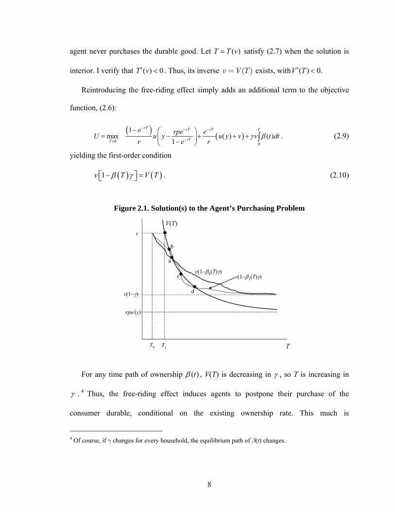
Figure 2.1. Solution(s) to the Agent’s Purchasing Problem
For any time path of ownership ( )tβ , V(T) is decreasing in γ , so T is increasing in
γ . 4 Thus, the free-riding effect induces agents to postpone their purchase of the
consumer durable, conditional on the existing ownership rate. This much is
4 Of course, if γ changes for every household, the equilibrium path of β(t) changes.
a
b
c
d
V(T)
v(1−γ)
v
rpu/(y)
T1T0 T
v(1−β0(T)γ)v(1−β1(T)γ)
9
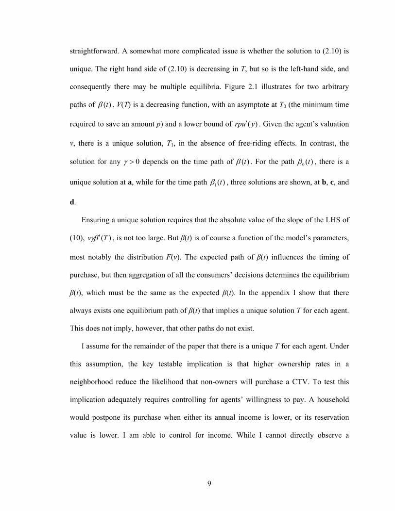
straightforward. A somewhat more complicated issue is whether the solution to (2.10) is
unique. The right hand side of (2.10) is decreasing in T, but so is the left-hand side, and
consequently there may be multiple equilibria. Figure 2.1 illustrates for two arbitrary
paths of ( )tβ . V(T) is a decreasing function, with an asymptote at T0 (the minimum time
required to save an amount p) and a lower bound of ( )rpu y′ . Given the agent’s valuation
v, there is a unique solution, T1, in the absence of free-riding effects. In contrast, the
solution for any 0γ > depends on the time path of ( )tβ . For the path 0 ( )tβ , there is a
unique solution at a, while for the time path 1( )tβ , three solutions are shown, at b, c, and
d.
Ensuring a unique solution requires that the absolute value of the slope of the LHS of
(10), ( )v Tγβ ′ , is not too large. But β(t) is of course a function of the model’s parameters,
most notably the distribution F(v). The expected path of β(t) influences the timing of
purchase, but then aggregation of all the consumers’ decisions determines the equilibrium
β(t), which must be the same as the expected β(t). In the appendix I show that there
always exists one equilibrium path of β(t) that implies a unique solution T for each agent.
This does not imply, however, that other paths do not exist.
I assume for the remainder of the paper that there is a unique T for each agent. Under
this assumption, the key testable implication is that higher ownership rates in a
neighborhood reduce the likelihood that non-owners will purchase a CTV. To test this
implication adequately requires controlling for agents’ willingness to pay. A household
would postpone its purchase when either its annual income is lower, or its reservation
value is lower. I am able to control for income. While I cannot directly observe a
10
household’s reservation value, I will examine several likely correlates, including the
stability of electricity, the quality of TV reception, and the electricity price, each of which
would influence the utility of TV consumption.
II.3. Data
The data used in this chapter are mainly from an October 1999 survey of rural durable
goods consumption conducted by the Rural Survey Organization (RSO), the National
Bureau of Statistics (NBS) of China.5 I also use data from the RSO’s regular annual
household survey of 1998. The consumption survey covered 20,000 households from all
the Chinese continental provinces except Tibet. They were drawn by a stratified random
sampling method from the RSO regular survey frame of about 68,300 households. The
survey was designed to assess the potential demand for durables in rural China. I exclude
from my sample the 0.7 percent of households with no power. Further eliminating
households with invalid data entries leaves me with around 18,800 households.
Since owning more than one CTV is rare in rural China, I follow convention in the
literature on the demand for durable goods (e.g. Dubin and McFadden (1984); Farrell
(1954)) and treat the demand for CTVs as a binary decision of buying or not. I also treat
CTV purchases in rural China during the 1990s as first purchases rather than
replacements. Before 1980, the start of China’s reform program, televisions were scarce
even in urban China, CTVs even more so. Most rural households didn’t purchase CTVs
until the 1990s. If the replacement cycle is 10 years or more, the assumption that most
5 Rong and Yao (2003) used the same data set to study the impact of public service provision on the rural consumption of electric appliances.
11
rural CTV purchases in the late 1990’s were first purchases seems reasonable. This
assumption is important because the external effect would be severely weakened if the
purchases recorded in the household survey were replacements. CTVs may have replaced
black and white sets, but in such cases I still treat CTV purchase as a first purchase.6
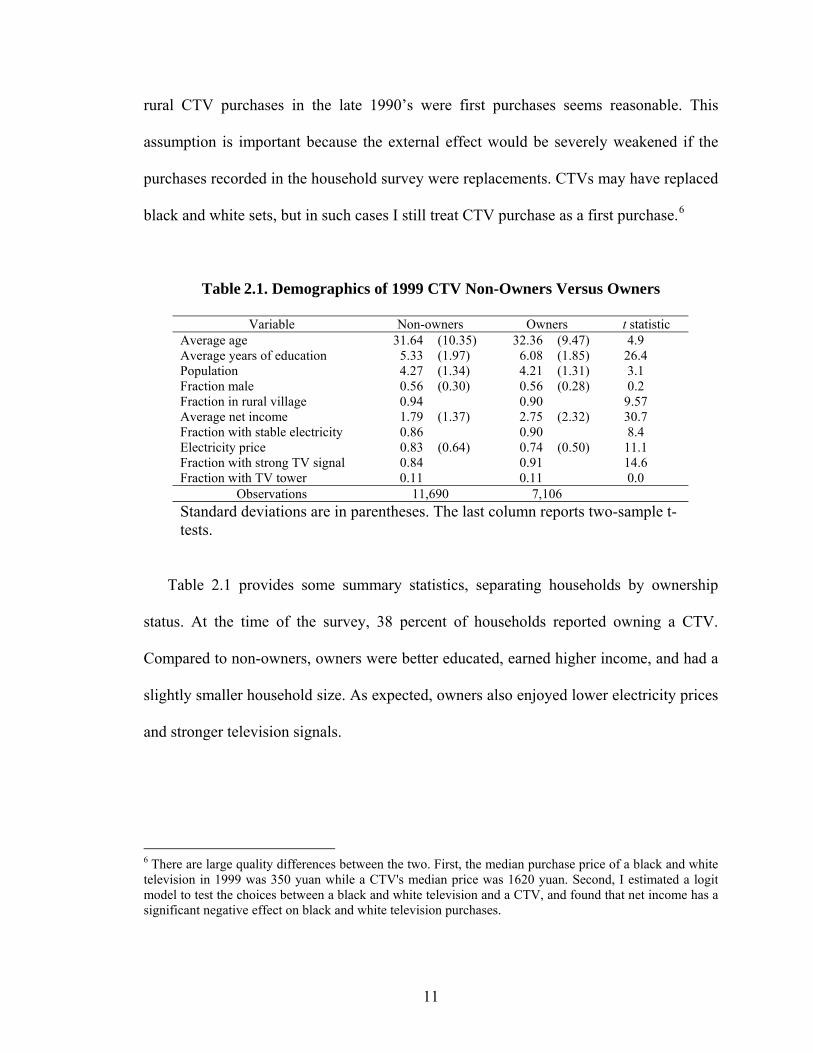
Table 2.1. Demographics of 1999 CTV Non-Owners Versus Owners
Variable Non-owners Owners t statistic Average age 31.64 (10.35) 32.36 (9.47) 4.9 Average years of education 5.33 (1.97) 6.08 (1.85) 26.4 Population 4.27 (1.34) 4.21 (1.31) 3.1 Fraction male 0.56 (0.30) 0.56 (0.28) 0.2 Fraction in rural village 0.94 0.90 9.57 Average net income 1.79 (1.37) 2.75 (2.32) 30.7 Fraction with stable electricity 0.86 0.90 8.4 Electricity price 0.83 (0.64) 0.74 (0.50) 11.1 Fraction with strong TV signal 0.84 0.91 14.6 Fraction with TV tower 0.11 0.11 0.0
Observations 11,690 7,106 Standard deviations are in parentheses. The last column reports two-sample t-tests.
Table 2.1 provides some summary statistics, separating households by ownership
status. At the time of the survey, 38 percent of households reported owning a CTV.
Compared to non-owners, owners were better educated, earned higher income, and had a
slightly smaller household size. As expected, owners also enjoyed lower electricity prices
and stronger television signals.
6 There are large quality differences between the two. First, the median purchase price of a black and white television in 1999 was 350 yuan while a CTV's median price was 1620 yuan. Second, I estimated a logit model to test the choices between a black and white television and a CTV, and found that net income has a significant negative effect on black and white television purchases.

12
II.4. Results
I analyze the effect of local ownership rates on CTV purchases using cross-sectional
probit regressions of household purchases on local ownership rates. The dependent
variable is a binary variable that equals one if a household purchased a CTV after the
initial year. The independent variable of interest is the village ownership rate before the
initial year. The ownership rate within a village is an ideal proxy for network effects.
However, I have on average fewer than ten households in each village, and as a result one
might be concerned that the sample village ownership rates are imprecise estimates of
their population means. To reduce this measurement error, I restrict my sample to
villages with at least ten observations when using the village ownership rate.7
My control variables are divided into three groups. The first group includes variables
describing household characteristics. They are household population, average age, the
fraction of the household that is male, average schooling years of members above sixteen
years of age, location of the household (town, suburban village, or rural village), and net
income per capita. Income measures the household’s budget constraint. All other
variables are intended to control for a household’s preference for electric appliances. The
location variable needs a little more elaboration. Location favors a rural household close
to a town in two ways. First, living in or close to a town provides households easy access
to the market and complementary services, and thus reduces its cost of buying and using
durable goods. Second, a household’s consumption style may be more like an urban
household if it lives in or close to a town.
7 I repeat the regressions with the sample of villages with at least 5 observations. I also run the regressions using the county-level ownership rate. In either case, the main results are persistent.

13
The second group collects variables describing the public service conditions enjoyed
by a household. They are binary variables for stability of the power supply (stable=1),
availability of tap water (yes=1), access to a TV signal receiving tower (yes=1), and TV
signal strength (good=1).8 Continuous controls in this group are the average prices of
electricity (in yuan/ kWh) and tap water (in yuan/ton) in 1997-99. If a village did not
have tap water, the average price in the county is used.
The third group of controls includes price indices for CTVs, as well as for
refrigerators, washing machines, bicycles, housing, fertilizers, and food. For CTVs,
refrigerators and washing machines, I calculate price indices from my survey data. The
remaining indices are constructed from RSO’s 1998 annual household survey. I am
unable to control for possible quality differences among the goods purchased by
households. I include province dummies to control for the fixed effect across provinces.
II.4.1. Initial Ownership Rates
To provide a complete picture of these regressions, I report in Table 2.2 the complete
sets of coefficients for CTV adoption since 1997. Half of the estimates are significant at
the one percent level, with signs consistent with expectations. In the group of family
characteristics, higher household population, greater average education, and higher
income increase a household’s probability of purchasing a CTV set. The effects of
average age and the fraction of the household that is male are not significant. The positive
effect of income is as expected. More family members reduce the cost per capita of 8 Power supply stability and TV signal strength are subjective measures. Since the survey did not provide respondents with clear definitions for these two variables, there may be considerable measurement error in these variables.

14
sharing a CTV, which increases the household’s willingness to buy. Higher educational
levels have two effects. First, people with more education tend to have a higher desire for
a modern living style. Second, more education implies easier adaptation to modern
technologies. Geographic location also matters. Households living in a rural village are
less likely to purchase than those in town or a suburban village. As expected, a stronger
TV signal makes a household more likely to purchase a CTV set. However, the effects of
electricity stability and electricity price are not significant.
Table 2.2. Probit Estimation of Purchasing CTV Sets since 1997
Standard Variable Coefficient Error
Intercept -3.29 *** 0.64 Average age -0.13 0.15 Average years of education 0.06 *** 0.01 Population 0.07 *** 0.01 Fraction male 0.06 0.06 Town dummy -0.08 0.11 Rural village dummy -0.2 *** 0.06 Average net income 0.09 *** 0.01 Electricity stability 0.05 0.06 Electricity price -0.01 0.02 Strength of TV signal 0.13 *** 0.05 Having TV tower or not 0 0.05 PI: bicycles 0.13 ** 0.06 PI: Housing -0.01 0.04 PI: Fertilizers 0.05 0.07 PI: Food 1.16 *** 0.15 PI: CTVs -0.03 0.09 PI: Refrigerators -0.17 0.37 PI: Washing machines 0.57 0.86 Ownership rate 0.83 *** 0.1 Province dummies Y
Mean Log-likelihood -0.49 Observations 10370
*, **, ***: Coefficient different from zero at 10, 5, 1 percent significance levels, respectively.

15
The results clearly show that a household was more likely to purchase a CTV set in a
given period when the ownership rate was higher at the beginning of the period. I change
the time scale and report the regressions in Table 2.3. The positive effect remains
significant. These indicate that either the free-riding effect did not influence household
CTV adoption or it was overwhelmed by the effect of network externalities.
Table 2.3. Effects of Initial Ownership Rates on CTV Adoption (Probit)
Adoption Adoption Adoption Adoption Adoption Variable 1998 1997 1996 1995 1994 (1) (2) (3) (4) (5)
Ownership rate 0.94 0.83 1.00 1.25 1.34 (0.10) (0.10) (0.14) (0.12) (0.14)
Mean log-likelihood -0.39 -0.49 -0.52 -0.54 -0.55 Observations 9423 10370 10904 11539 11844
Notes: Standard errors are in parentheses. Each column regresses the decision to buy a CTV starting at the beginning of 1998-1994, respectively.
If it is the case that free riding influenced CTV adoption but was overwhelmed, one
should expect that the estimated coefficient on the ownership rate in regressions of either
washing machine or refrigerator adoption will be larger than for CTV because it is
unlikely that neighbors share the former two durable goods. Table 2.4 reports results
from probit regressions of washing machine and refrigerator adoption since 1997. As
expected, the estimated coefficient on the initial ownership rate in the regression of CTV
adoption is significantly lower than the other two. Since coefficient values are hard to
compare across probit regressions, Table 2.4 also reports the logit and linear probability
regression, respectively. The differences are persistently significant.
16
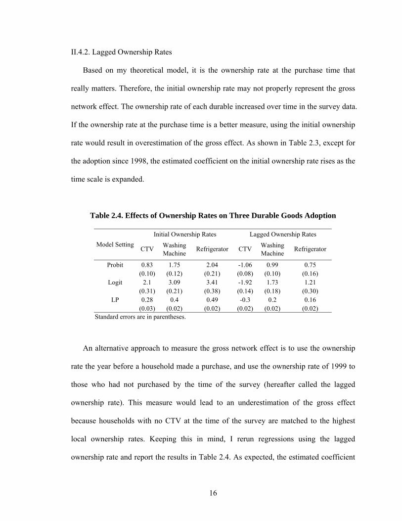
II.4.2. Lagged Ownership Rates
Based on my theoretical model, it is the ownership rate at the purchase time that
really matters. Therefore, the initial ownership rate may not properly represent the gross
network effect. The ownership rate of each durable increased over time in the survey data.
If the ownership rate at the purchase time is a better measure, using the initial ownership
rate would result in overestimation of the gross effect. As shown in Table 2.3, except for
the adoption since 1998, the estimated coefficient on the initial ownership rate rises as the
time scale is expanded.
Table 2.4. Effects of Ownership Rates on Three Durable Goods Adoption
Initial Ownership Rates Lagged Ownership Rates
Washing Washing Model Setting CTV
Machine Refrigerator CTV
Machine Refrigerator
Probit 0.83 1.75 2.04 -1.06 0.99 0.75 (0.10) (0.12) (0.21) (0.08) (0.10) (0.16)
Logit 2.1 3.09 3.41 -1.92 1.73 1.21 (0.31) (0.21) (0.38) (0.14) (0.18) (0.30)
LP 0.28 0.4 0.49 -0.3 0.2 0.16 (0.03) (0.02) (0.02) (0.02) (0.02) (0.02) Standard errors are in parentheses.
An alternative approach to measure the gross network effect is to use the ownership
rate the year before a household made a purchase, and use the ownership rate of 1999 to
those who had not purchased by the time of the survey (hereafter called the lagged
ownership rate). This measure would lead to an underestimation of the gross effect
because households with no CTV at the time of the survey are matched to the highest
local ownership rates. Keeping this in mind, I rerun regressions using the lagged
ownership rate and report the results in Table 2.4. As expected, the estimated coefficient

17
on the ownership rate in the regression of CTV adoption decreases significantly and in
fact becomes negative. In contrast, although they too decline, the corresponding
coefficient for washing machine and refrigerator adoption remain significantly positive.
Both are consistent with the hypothesis of that there is a free-riding effect in CTV
adoption.
In Table 2.5 I report two robustness tests of the negative effect of the lagged
ownership rate on CTV adoption. To save space, I again restrict attention to purchases
made since 1997. To ensure that results are not driven by excessive variation in reported
income, I keep only those households whose income is within one standard deviation of
the mean. The result is reported in column 1 of Table 2.5. The effect of the lagged
ownership rate remains significantly negative after the refinement.
I next add more variables that are plausibly correlated with a household’s purchase
decision. If the results are due to unobserved factors, adding these variables should
reduce the effect of the lagged ownership rate. In column 2 of Table 2.5, I add three
interactions of the demographic variables (income*education, education*age, and
income*age), and three dummies for ownership of other electrical appliances (black and
white televisions, washing machines, and refrigerators). I have no particular expectations
for the coefficients on the interaction terms, so they are suppressed in the table. As one
should expect, ownership of a black and white television reduces the likelihood that the
household owns a CTV. In contrast, households that own a washing machine or a
refrigerator are more likely also to own a CTV. I conjecture that ownership of these other
appliances is correlated with unobserved household characteristics that affect the
likelihood of durable purchases. It is notable that addition of these additional controls
18
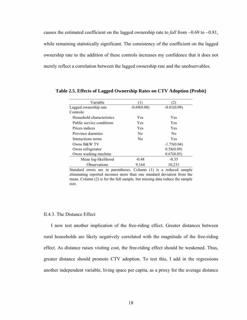
causes the estimated coefficient on the lagged ownership rate to fall from −0.69 to −0.81,
while remaining statistically significant. The consistency of the coefficient on the lagged
ownership rate to the addition of these controls increases my confidence that it does not
merely reflect a correlation between the lagged ownership rate and the unobservables.
Table 2.5. Effects of Lagged Ownership Rates on CTV Adoption (Probit)
Variable (1) (2) Lagged ownership rate -0.69(0.08) -0.81(0.09) Controls: Household characteristics Yes Yes Public service conditions Yes Yes Prices indices Yes Yes Province dummies No No Interactions terms No Yes Owns B&W TV -1.75(0.04) Owns refrigerator 0.58(0.09) Owns washing machine 0.67(0.05)
Mean log-likelihood -0.48 -0.35 Observations 9,164 10,231
Standard errors are in parentheses. Column (1) is a reduced sample eliminating reported incomes more than one standard deviation from the mean. Column (2) is for the full sample, but missing data reduce the sample size.
II.4.3. The Distance Effect
I now test another implication of the free-riding effect. Greater distances between
rural households are likely negatively correlated with the magnitude of the free-riding
effect. As distance raises visiting cost, the free-riding effect should be weakened. Thus,
greater distance should promote CTV adoption. To test this, I add in the regressions
another independent variable, living space per capita, as a proxy for the average distance
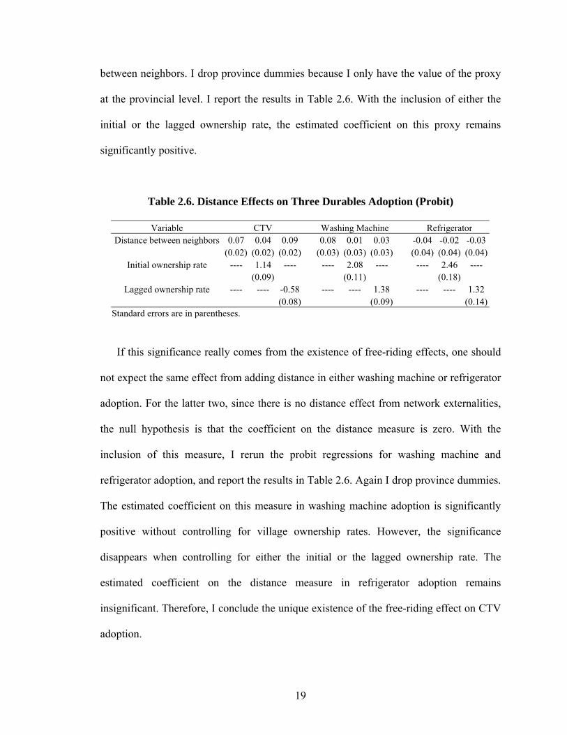
19
between neighbors. I drop province dummies because I only have the value of the proxy
at the provincial level. I report the results in Table 2.6. With the inclusion of either the
initial or the lagged ownership rate, the estimated coefficient on this proxy remains
significantly positive.
Table 2.6. Distance Effects on Three Durables Adoption (Probit)
Variable CTV Washing Machine Refrigerator Distance between neighbors 0.07 0.04 0.09 0.08 0.01 0.03 -0.04 -0.02 -0.03
(0.02) (0.02) (0.02) (0.03) (0.03) (0.03) (0.04) (0.04) (0.04)Initial ownership rate ---- 1.14 ---- ---- 2.08 ---- ---- 2.46 ----
(0.09) (0.11) (0.18) Lagged ownership rate ---- ---- -0.58 ---- ---- 1.38 ---- ---- 1.32
(0.08) (0.09) (0.14)Standard errors are in parentheses.
If this significance really comes from the existence of free-riding effects, one should
not expect the same effect from adding distance in either washing machine or refrigerator
adoption. For the latter two, since there is no distance effect from network externalities,
the null hypothesis is that the coefficient on the distance measure is zero. With the
inclusion of this measure, I rerun the probit regressions for washing machine and
refrigerator adoption, and report the results in Table 2.6. Again I drop province dummies.
The estimated coefficient on this measure in washing machine adoption is significantly
positive without controlling for village ownership rates. However, the significance
disappears when controlling for either the initial or the lagged ownership rate. The
estimated coefficient on the distance measure in refrigerator adoption remains
insignificant. Therefore, I conclude the unique existence of the free-riding effect on CTV
adoption.
20
II.5. Conclusions
Motivated by the observation that CTV owners in rural China typically welcome their
non-owner neighbors to watch television with them, I set out to evaluate how this free
riding would influence CTV adoption. I constructed a model of the timing of purchasing
a durable good in the presence of this free-riding effect, and showed that the stronger the
effect and the greater the local ownership rate, the more likely a non-owner is to postpone
purchase.
Using micro level data on nearly 19,000 rural China households surveyed in 1999, I
produce evidence that the free-riding effect exists in household CTV adoption. Because
of the coexistence of network externalities and free riding, I find that the greater the
initial ownership rate, the more likely a non-owner is to purchase a CTV. However, the
estimated coefficient on initial ownership rates is significantly lower than that in either
washing machine or refrigerator adoption. These differences are similar across different
specifications. Moreover, when I estimate CTV adoption using the lagged ownership rate,
its estimated coefficient turns to be significantly negative. The negative sign persists with
the inclusion of numerous controls. I fail to detect this change in sign when I estimate
washing machine and refrigerator adoption using the lagged ownership rate. These results
are consistent with the hypothesis that the free-riding effect exists in CTV adoption in
rural China.
I further test another implication of the free-riding effect. Greater distances between
rural households are likely negatively correlated with the magnitude of the free-riding
effect. Controlling for the ownership rate, the distance effect on CTV adoption is
significantly positive. In contrast, it is insignificant in washing machine or refrigerator

21
adoption. While this effect is not evident in the data for washing machines and
refrigerators, it is likely not unique to rural CTV adoption. Other durable goods with the
characteristic of a public good should lead to similar results. One notable example is that
of local phone service.
22
References
Bandiera, O., and I. Rasul (2006): “Social Networks and Technology Adoption in Northern Mozambique.” The Economic Journal, 116(514):869–902.
Berndt, E. R., R. S. Pindyck, and P. Azoulay (2000): “Consumption Externalities and Diffusion in Pharmaceutical Markets: Antiulcer Drugs.” NBER Working Paper No. 7772.
Dubin, J. A., and D. McFadden (1984): “An Econometric Analysis of Residential Electric Appliance Holdings and Consumption.” Econometrica, 52(2):345-362.
Farrell, M. J. (1954): “The Demand for Motor Cars in the United States.” Journal of the Royal Statistical Society, Series A, 117(2):171-201.
Gandal, N. (1994): “Hedonic Price Indexes for Spreadsheets and an Empirical Test for Network Externalities.” RAND Journal of Economics, 25(2):160-170.
Goolsbee, A., and P. J. Klenow (2002): “Evidence on Learning and Network Externalities in the Diffusion of Home Computers.” Journal of Law and Economics, 45(2):317-343.
Gowrisankaran, G., and J. Stavins (2004): “Network Externalities and Technology Adoption: Lessons from Electronic Payments.” RAND Journal of Economics, 35(2):260-276.
Karshenas, M., and P. L. Stoneman (1993): “Rank, Stock, Order, and Epidemic Effects in the Diffusion of New Process Technologies: An Empirical Model.” Rand Journal of Economics, 24:503--28.
Leahy, J. V., and J. Zeira (2005): “The Timing of Purchases and Aggregate Fluctuations.” Review of Economic Studies, 72(6):1127-1151.
Liebowitz, S. J., and S. E. Margolis (1994): “Network Externality: An Uncommon Tragedy.” Journal of Economic Perspectives, 8(2):133-150.
Manski, C. F. (1993): “Identification of Endogenous Social Effects: The Reflection Problem”, Review of Economic Studies, 60(3):531-542.
Park, S. (2004): “Quantitative Analysis of Network Externalities in Competing Technologies: The VCR Case.” Review of Economics and Statistics, 86(4):937-945.
Rong, Z., and Y. Yao (2003): “Public Service Provision and the Demand for Electric Appliances in Rural China.” China Economic Review, 14(2):131-141.

23
Appendix
If there is a unique solution to equation (2.10) for any v, then ( )tβ is uniquely
defined for all t. The ownership rate must satisfy
[ ]
( )
min
min
0, 0,( )
( )1 , ,
1 ( )
t Tt
V tF t T
t
β
β γ
∈=
− ∈ ∞−
⎧⎪⎪⎨⎪ ⎛ ⎞
⎜ ⎟⎪ ⎝ ⎠⎩
, (2.A1)
where ( )1min ln ( ) /T r rp y y−= + . I need only consider values of mint T≥ . It is easy to verify
that
11
VFβ
βγ= −
−⎛ ⎞⎜ ⎟⎝ ⎠
(2.A2)
has a unique solution for any given V . The LHS of (2.A2) is increasing in β while the
RHS is decreasing. At 0β = , the RHS is ( ) 0.F V β≥ = At 1β = the RHS is (1
)VFγ−
1.β≤ = Since both functions are continuous, there exists a unique solution
( ) [0,1]Vβ ∈ satisfying (2.A2). But as V(t) is uniquely defined for any mint T≥ then
( ) [0,1]tβ ∈ is uniquely defined for all mint T≥ .
24
III. DO INSIDER TRADING PATTERNS PREDICT A FIRM’S PATENT OUTPUT?
III.1. Introduction
Numerous studies have documented that “corporate insiders”9 earn excess returns
from trading the securities of their firms (e.g., Jaffe (1974); Finnerty (1976); Seyhun
(1986)). However, the specific sources of information asymmetry that lead to insider
gains have not been comprehensively investigated. Aboody and Lev (2000) demonstrate
that R&D is a major contributor to information asymmetry by finding that insider gains in
R&D intensive firms are substantially larger than those in firms that conduct little
R&D. 10 They argue that the uniqueness of R&D investments 11 makes it difficult for
outsiders to learn about the productivity of a given firm’s R&D. The absence of
organized R&D markets and the ambiguity of R&D accounting rules further exacerbate
the information asymmetry associated with R&D.
It is interesting to further ask how each R&D-related source contributes to
information asymmetry. This chapter explores a potential source, the value of a firm’s
patent output, which has been widely used to measure a firm’s R&D success. The value
of patent output (hereafter patent output) refers to the discounted present value of a firm’s
9 Corporate insiders are defined by the 1934 Securities and Exchange Act as corporate officers, directors, and owners of 10 percent or more of any equity class of securities.
10 There is other empirical evidence consistent with a relatively large information asymmetry associated with R&D. Barth, Kasznik, and McNichols (1998) report that analyst coverage is significantly larger for R&D intensive firms. Similarly, Tasker (1998) reports that R&D intensive firms conduct more conference calls with analysts than less R&D intensive firms.
11 According to Kothari, Laguerre, and Leone (1998), in the regression of future earnings variability on investment in R&D, PP&E (property, plant, and equipment), and other determinants of earning variability like firm size and leverage, the coefficient on R&D is three times as large as that on PP&E.

25
future net cash flow contributed by its granted patents. Since it is practically impossible
to distinguish the contribution of patents from many other factors, a considerable
literature uses the count of granted patents as a proxy for R&D success (e.g., Scherer
(1965); Schmookler (1966); Griliches (1995)). But this proxy is limited by the large
variance in the value of individual patents. One way to account for this heterogeneity is to
use citation-weighted patent counts. That is, a firm’s patent counts are supplemented with
the number of subsequent citations.12
Patents are economically valuable, and their potential impact on firm value has been
recognized by investors in the stock market. Empirical evidence shows that patent value
is partially reflected in the stock price before relevant information is fully released. Hall,
Jaffe, and Trajtenberg (2005) report that the market value of a listed firm is positively
correlated with the portion of forward citations that cannot be predicted based upon past
citations of its granted patents. Deng, Lev, and Narin (1999) find that the number of
granted patents and patent citations are strongly related to investors’ growth expectations
in the chemicals, drugs, and electronics industries. Given this recognition by investors, it
is interesting to ask whether management possesses information about its patent output
beyond what is known to investors. However, as far as I know little evidence has been
provided on this question.
In this chapter I use corporate insider trading records during the period of patent
application to test whether management possesses privileged information about its patent
output. I only include corporate officers and directors, which are regarded as the
12 See Section III.3 for a detailed discussion on measures of patent output.

26
management. Hereafter, “insider trading” refers to corporate officers and directors trading
in their own stocks, which has been reported to the SEC. The motivation for examining
insider trading records is that the information management has about patent output, but
that is not known to other market participants, is likely to be reflected in insider trading
when management exploits its information advantage in the stock market.
Specifically, I ask whether, given market reactions, insider trading patterns have
significant effects on predicting patent output. To analyze this question, I examine
regressions of patent output on insider trading patterns and abnormal stock returns. I find
that management possesses statistically significant additional information. Moreover, the
predictive power of insider trading patterns on patent output comes from purchases while
insider sales appear to have little predictive power. These findings are similar across
different measures of patent output, across different time scales, and across different
measures of insider trading patterns.
This chapter is organized as follows. Section III.2 develops a two-stage estimation
model. Section III.3 describes the data and variables. Section III.4 reports the empirical
results. Section III.5 concludes.
III.2. Estimation Settings
The rational expectations hypothesis implies that investors react only to unexpected
shocks. The occurrence of a fully expected event should not influence investment
behavior, and hence should have no impact on the stock price. The same logic applies to
patent output. Both management and investors react only when they observe unexpected
fluctuations of patent output. To examine the relationship between insider trading
27
patterns and a firm’s patent output, one should first estimate the unexpected portion of
this output.
Pakes and Grilliches (1980) provide an empirical model to estimate the relationship
between patents applied for and R&D expenditures. A statistically significant relationship
has been found. I use a similar model here to estimate market expectations about a firm’s
patent output given the current R&D expenditures. I choose a linear production function
instead of Cobb-Douglas because OLS estimation results show that the R² with the linear
function is higher.13 I ignore the lagged effects of R&D expenditures in light of the
finding of Hall, Griliches, and Hausman (1986) that the contribution of the observed
R&D history to the current year’s patent application is quite small. Thus, the first-stage
estimation model is as follows.
1 2
1, 1 , ,' 'i t i t i t i tPC RD FIRM YEARα θ η η ε= + + + + (3.1)
where ,i tPC is a measure of firm i’s patent output in year t. It is not directly observable in
year t because no one knows the future net cash flow that these patents will contribute to.
,i tRD is the R&D expenditures in year t. It measures firm i’s patent-related R&D
investment. iFIRM is a vector of firm dummies to control for the fixed effects across
firms. iYEAR is a vector of year dummies to control for annual differences of the patent
granting process. 1,i tε includes the contribution of ignored factors, such as managerial
skills in R&D process, and uncertainty in R&D investment. They are not publicly
observable.
13 Redoing the regressions using the Cobb-Douglas function has little effect on the main results.

28
In the second stage, I use the difference between the realized and the estimated patent
output from model (3.1), ( , ,i t i tPC PC∧
− ) to measure the unexpected portion of patent
output. Management should not react promptly to ( , ,i t i tPC PC∧
− ) unless it has
considerable information about the realized patent output, ,i tPC . Thus, if the effects of
contemporary insider trading patterns are significant to explain ( , ,i t i tPC PC∧
− ), it would
indicate that management does have timely considerable information about ,i tPC .
Since my interest is in management’s timely knowledge about realized patent output,
I only include insider trading measures in the years around the observation year. Those
measures in the later years may help to explain ( , ,i t i tPC PC∧
− ) either because additional
information about patent value is gradually released or because management strategically
delays its reaction. Because it is impossible to distinguish between these two effects, I
ignore the possible delay effect and focus on examining contemporary insider activities. I
use the following empirical model to examine how insider trading patterns explain
( , ,i t i tPC PC∧
− ).
1 1
2, , 2 , , ,
1 1i t i t j i t j j i t j i t
j j
PC PC IP ISα β γ ε∧
+ +=− =−
− = + + +∑ ∑ (3.2)
where the insider purchase measures, IP and insider selling measures, IS from year 1t −
to 1t + are included. I treat insider purchases and insider sales separately in case that they
have different explanatory power. Several empirical studies have revealed this difference.
By examining listed companies for 1975-95, Lakonishok and Lee (2001) find that the
informative of insider activities in predicting stock returns comes from purchases while

29
insider sales appear to have no predictive power. Jeng, Metrick, and Zeckhauser (2003)
report that for a one year holding period insider gains on purchases are 0.4 percent
abnormal returns per month while the abnormal returns for sales are insignificant.
Admittedly, this approach may not reveal management’s knowledge about the
realized patent output. Insider trading patterns should reflect the aggregation effect of all
shocks during the period, among which fluctuations in patent output may be a small part.
However, as long as we detect significant estimated coefficients on either IP or IS in
model (3.2), we should confirm management’s timely considerable information about
patent output. Even if the effects of insider trading patterns are significant to explain
( , ,i t i tPC PC∧
− ) in model (3.2), it is still unclear whether management knows better about
patent output than investors.
An alternative explanation is that management follows the market, and the market
knows about ( , ,i t i tPC PC∧
− ). To reject this hypothesis, I then test whether management
possesses considerable information about patent output beyond what is known to
investors. Romer and Romer (2000) find out that the Federal Reserve has considerable
information about inflation beyond what is known to commercial forecasters by
examining whether individuals who know the commercial forecasts could make better
forecasts if they also knew the Federal Reserve’s. I use a similar approach by testing
whether investors who know the market reactions would know better about
( , ,i t i tPC PC∧
− ) if they also knew insider trading patterns. The empirical model is as
follows.

30
1 1
, , 3 , ,1 1
i t i t j i t j j i t jj j
PC PC IP ISα β γ∧
+ +=− =−
− = + +∑ ∑
( )4
3, ,
1
mj i t j t j i t
j
R Rδ ε+ +=−
+ − +∑ (3.3)
where the abnormal returns from year 1t − to 4t + are included. These measure the
market reactions around the patent application period as well as in the later years.14 ,i tR is
the rate of return on firm i’s stock in year t. mtR is the S&P Industrial Index annual return
in year t. If any estimated coefficient on either IP or IS in model (3.3) remains significant,
I would reject the null hypothesis that management knows about patent output no more
than the market while accepting that it knows better.
Model (3.3) would be seriously flawed if the interaction between management and
investors is significant. Fortunately, this problem is minor due to their weak relationship
revealed by empirical evidence. Lakonishok and Lee (2001) find that little market
movement is observed when insiders trade or when they report their trades to the SEC.
Seyhun (1986) and Rozeff and Zaman (1988) show that, net of transaction costs,
investors do not benefit by imitating insiders.15
III.3. Data and Variables
The variables used in this chapter are extracted from three major data sources. One is
patent data from the NBER, which includes information on granted patents and their
14 Redoing the regressions using different length of leads in abnormal returns has little effect on the results.
15 It is still debatable whether investors can profit from knowing what insiders are doing. Bettis, Vickrey, and Vichrey (1997) show that investors can earn abnormal returns, net of transaction costs, by analyzing publicly available information about transactions by top management.
31
citations. Another is firm-level financial data from the Compustat annual company files.
Both active and subsequently delisted companies are included. The last are insider
trading data starting at 1986 from the Thomson Financial (TFN), containing all purchase
and sales transactions made by insiders and reported to the SEC.
If insiders react to fluctuations of patent output, it would be more likely to happen in
R&D intensive firms where fluctuations are much stronger. For this reason, I focus on
examining R&D intensive firms. In the analysis, I only include firms whose average
patent annual counts (hereafter PACs) for 1986-94 are greater than 30. The PACs refer to
the number of granted patents that are applied for in a given year. After excluding firms
with no insider trading record, I end up with 88 firms.16
III.3.1. Dependent Variable: Patent Output
Before November 2000, patent applications in the US were kept secret until the patent
issues. 17 The USPTO only published the granted patents. Access to pending patent
applications in the USPTO was governed by 35 USC 122, which states:
Applications for patents shall be kept in confidence by the Patent and
Trademark Office and no information concerning the same given without
authority of the applicant or owner unless necessary to carry out the
provisions of any Act of Congress or in such special circumstances as may
be determined by the Commissioner.
16 A list of the 88 firms is in the Appendix.
17 After 2000, patent applications in the USPTO are required to publish within 18 months after the earliest date of the application. Even so, management's foreknowledge of patent applications is still apparent.
32
Since the invention date of a patent is not available, I treat its application date as its
invention date. Proxies are used to measure patent output by examining granted patents,
valid patents18, international patent applications, or patent citations (Earnst (1999)) due to
the absence of an organized patent market. To measure the realized patent output, I count
the number of granted patents that are applied for in a given year, which comes to be
PACs.
A truncation bias is involved in patent counting. In a later year a larger fraction of
patent applications are likely to stay in the examination process. Thus, fewer patents are
expected to appear in the data set. My last observation year is 1994, with granting records
until 1999 as the reference. This truncation bias is ignorable because the likelihood that a
1994 patent application still stayed in the examination process in 1999 was rare.19
According to the USPTO website, a lag between the application time and the granted
time (hereafter called grant lag) is 24.6 months on average. The grant rate historically
was about 66%, which has dropped to 54% recently, as claimed by the USPTO.
Therefore, the current PACs were unobservable to either management or investors.
The fluctuation in PACs is hard to predict within a firm. Pakes and Grilliches (1980)
find that R&D expenditures can only explain on average 20-30% of the volatility of
PACs in the within-firm time-series dimension. This percentage is expected to be even
lower in R&D intensive firms in which PACs are more volatile.
18 A patent is valid if it has been previously granted and its protection fee is still paid.
19 According to Hall, Jaffe, and Trajtenberg (2001), less than 2% of applications submitted during 1990-92 had a grant lag of more than 4 years.
33
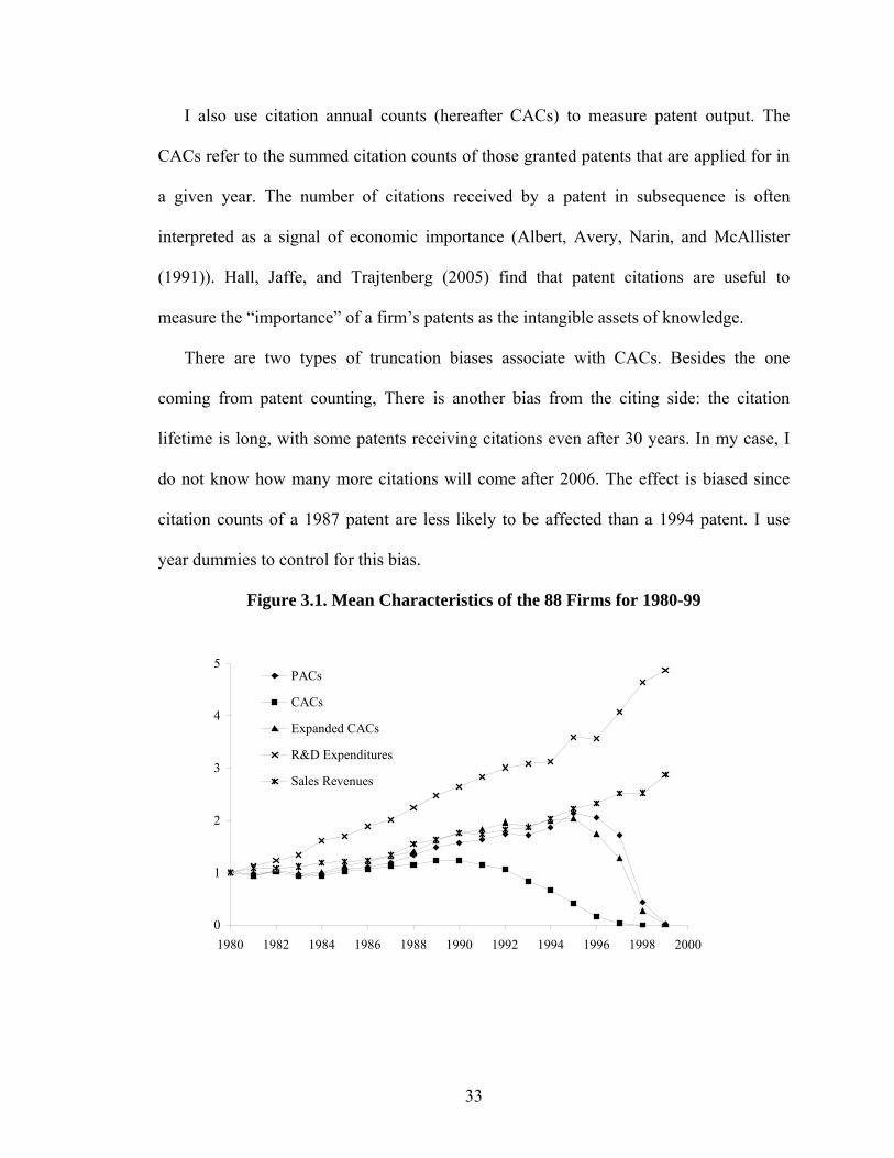
I also use citation annual counts (hereafter CACs) to measure patent output. The
CACs refer to the summed citation counts of those granted patents that are applied for in
a given year. The number of citations received by a patent in subsequence is often
interpreted as a signal of economic importance (Albert, Avery, Narin, and McAllister
(1991)). Hall, Jaffe, and Trajtenberg (2005) find that patent citations are useful to
measure the “importance” of a firm’s patents as the intangible assets of knowledge.
There are two types of truncation biases associate with CACs. Besides the one
coming from patent counting, There is another bias from the citing side: the citation
lifetime is long, with some patents receiving citations even after 30 years. In my case, I
do not know how many more citations will come after 2006. The effect is biased since
citation counts of a 1987 patent are less likely to be affected than a 1994 patent. I use
year dummies to control for this bias.
Figure 3.1. Mean Characteristics of the 88 Firms for 1980-99
0
1
2
3
4
5
1980 1982 1984 1986 1988 1990 1992 1994 1996 1998 2000
PACs
CACs
Expanded CACs
R&D Expenditures
Sales Revenues
34
Figure 3.1 shows some mean characteristics of the 88 firms for 1980-99 in Figure 3.1.
Each variable is normalized by dividing by its 1980 value. R&D expenditures increased
four-fold from 1980 to 1999 while sales increased only 2-fold. The upward trend in PACs
reversed in 1995. The same reverse in CACs happened in 1990. These are because the
granting records in the NBER data stop in 1999. For the same reason, both variables
dropped to near zero in 1999.
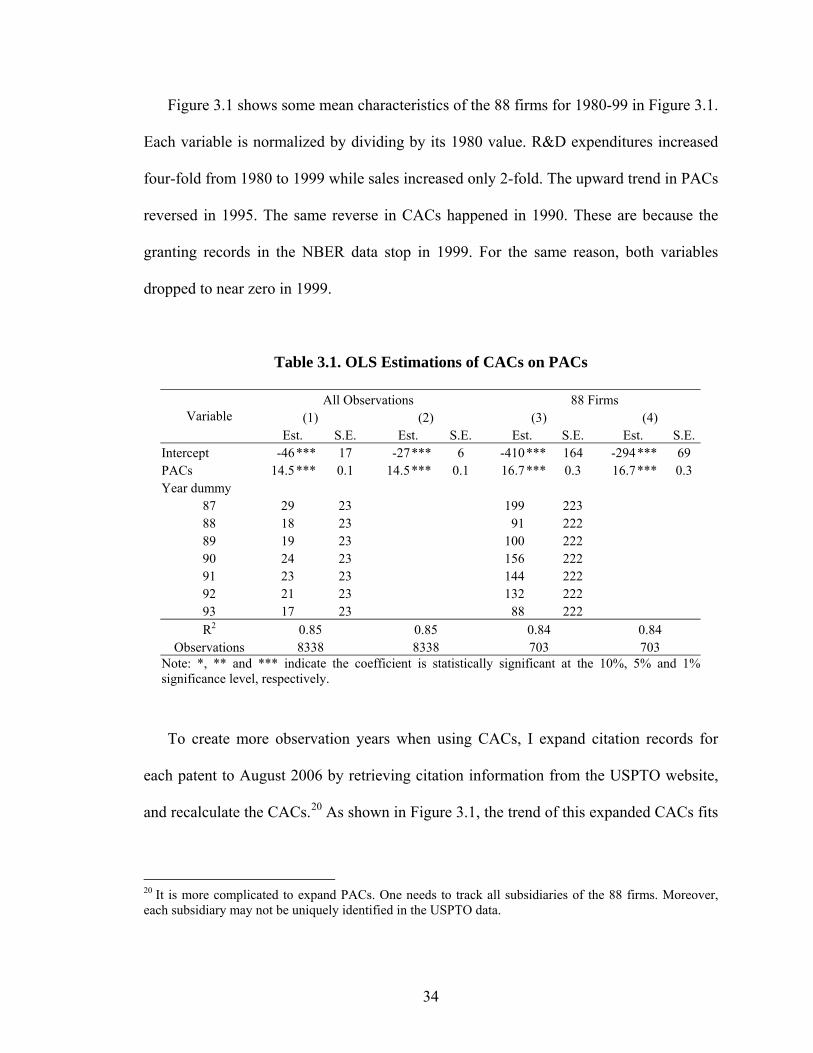
Table 3.1. OLS Estimations of CACs on PACs
All Observations 88 Firms (1) (2) (3) (4) Variable
Est. S.E. Est. S.E. Est. S.E. Est. S.E.Intercept -46 *** 17 -27*** 6 -410*** 164 -294 *** 69 PACs 14.5 *** 0.1 14.5*** 0.1 16.7*** 0.3 16.7 *** 0.3 Year dummy
87 29 23 199 223 88 18 23 91 222 89 19 23 100 222 90 24 23 156 222 91 23 23 144 222 92 21 23 132 222 93 17 23 88 222 R2 0.85 0.85 0.84 0.84
Observations 8338 8338 703 703 Note: *, ** and *** indicate the coefficient is statistically significant at the 10%, 5% and 1% significance level, respectively.
To create more observation years when using CACs, I expand citation records for
each patent to August 2006 by retrieving citation information from the USPTO website,
and recalculate the CACs.20 As shown in Figure 3.1, the trend of this expanded CACs fits
20 It is more complicated to expand PACs. One needs to track all subsidiaries of the 88 firms. Moreover, each subsidiary may not be uniquely identified in the USPTO data.
35
well with the PACs till 1995.21 I only use the expanded CACs in my estimations for
1987-94.
To better understand the relationship between PACs and CACs, I run the OLS
estimations of CACs on PACs for the years 1987-94 and report the results in Table 3.1. I
first use all observations that have at least one PAC. In column (1), I include year
dummies to control for the second truncation bias. It shows that the model explains 85%
of the volatility in CACs. The estimated coefficient on PACs is significantly positive
while those on year dummies are insignificant. I test the null hypothesis that each
coefficient on year dummies is zero and fail to reject the null at the significance level of
10%. Thus, the effect of the second truncation bias is negligible. In column (2) I exclude
year dummies. The effect of PACs remains significant with the same R². In column (3)
and (4), I repeat the estimations using the 88-firm observations with at least one PAC.
The R² is slightly lower while the estimated coefficient on PACs increases by 15%,
indicating higher citation counts per patent in R&D intensive firms.22
Though they are similar, these two measures are different in information utilization.
Hall, Jaff and Trajtenberg (2001) document that it took over 10 years for a 1975 patent to
receive 50% of its citations, the total of which is measured within a 35-year time
21 To check the correctness of the citation data that I retrieve from the USPTO website, I compare it with the NBER data by examining the patents with patent number from 6000001 to 6009554. It turns out that my data is quit precise with respect to the NBER data. I find 4 patents with citation errors, with an error rate of only 0.04%. Among them, 3 patents have citations incomplete because a rare situation is not taken into account in my program, and 1 patent has no citation due to the download problem. Since the error rate is within tolerance and no sampling bias is expected, I use the data as it is. Comparatively, the NBER data has 15 patents with errors, of which 10 patents have been withdrawn and 5 have updated citations.
22 It may be because R&D intensive firms tend to focus on more influential R&D programs. Or it may simply reflect that the distribution of citation counts is right-skewed.

36
window.23 In my case, CACs utilize citation records for at least 12 years. Comparatively,
more than 95% of patent applications during 1973-75 were granted in four years.
III.3.2. Independent Variable: Insider Trading Patterns
Insiders were required to inform the SEC of any trades in the firm’s stock by filing a
“Statement of Change in Beneficial Ownership of Securities” form by the tenth of the
month24 following the month in which they trade. Trading on privileged information is
illegal, by Sections 17(a) and 10(B) of the Securities and Exchange Act of 1934 and SEC
Rule 10(b)-5. However, since patent applications are submitted frequently in an R&D
intensive firm, insider trading based on them is less likely to face legal jeopardies.25
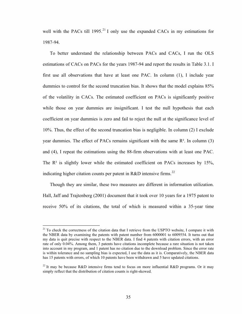
Table 3.2 summarizes the transaction counts of each insider type for 1987-94.26 The
Vice President, Officer, and Director are the three types who engage in the heaviest
trading. They account for 73% of the total counts. Since my interest is in management, I
exclude the following personals: SH, AF, B, UT, T, R, TR, GC, CP, AI, and IA. About
6% of the total transaction counts are eliminated.
23 It would be useful to know how reliable it is to estimate a firm’s life-time (say 35 years) CACs by examining the CACs of the first 10 years. Unfortunately, no one did it so far as I know.
24 Effective on August 29, 2002, insiders must report to the SEC certain changes in their beneficial ownership of their company's securities within 2 business days after the date of the transaction.
25 Insider trading has been found in many corporate events, such as bankruptcy (Seyhun and Bradley (1997)), dividend initiation (John and Lang (1991)), seasoned equity offerings (Karpoff and Lee (1991)), stock repurchases (Lee, Mikkelson, and Parch (1992)), and takeover (Seyhun (1990)).
26 See TFN Insider Filing Data for details.
37
Table 3.2. Transaction Counts for Insider Types
Code Count Percentage Description VP 40060 37.77 Vice President O 22501 21.21 Officer D 14749 13.91 Director OX 6532 6.16 Divisional Officer OD 5092 4.80 Officer and Director CB 4838 4.56 Chairman of the Board P 3070 2.89 President * SH 2655 2.50 Shareholder * AF 1542 1.45 Affiliated Person (A person who is able to exert influence on a
corporation, often as a result of minority ownership.)
OS 1538 1.45 Officer of Subsidiary Company * B 1520 1.43 Beneficial Owner of more than 10% of a Class of Security MC 570 0.54 Member of Committee or Advisory Board CF 294 0.28 Chief Financial Officer * UT 269 0.25 Unknown * T 221 0.21 Trustee OT 180 0.17 Officer and Treasurer H 142 0.13 Officer, Director and Beneficial Owner * R 97 0.09 Retired DO 53 0.05 Director and Beneficial Owner of more than 10% of a Class of Security CE 35 0.03 Chief Executive Officer * TR 28 0.03 Treasurer CO 23 0.02 Chief Operating Officer CEO 16 0.02 Chief Executive Officer GM 13 0.01 General Manager * GC 8 0.01 General Counsel VC 8 0.01 Vice Chairman F 6 0.01 Founder * CP 3 0.00 Controlling Person ("Control” means ownership of, or the power to vote,
twenty-five percent (25%) or more of the outstanding voting securities of a licensee or controlling person.)
* AI 1 0.00 Affiliate of Investment Advisor CFO 1 0.00 Chief Financial Officer * IA 1 0.00 Investment Advisor
Sum 106063 100 Note: * indicates the type is eliminated. There are 12 trading records with the code empty.
Table 3.3 summarizes the counts of each transaction type for 1987-94. I only take into
account two of them: P and S, which represent “open market or private purchase of non-
derivative or derivative security” and “open market or private sale of non-derivative or
derivative security”, respectively. Even though these definitions do not preclude the
38
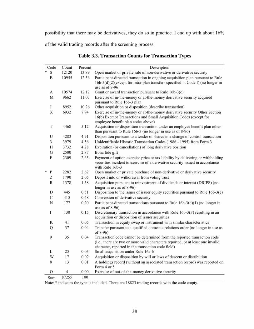
possibility that there may be derivatives, they do so in practice. I end up with about 16%
of the valid trading records after the screening process.
Table 3.3. Transaction Counts for Transaction Types
Code Count Percent Description * S 12120 13.89 Open market or private sale of non-derivative or derivative security B 10955 12.56 Participant-directed transaction in ongoing acquisition plan pursuant to Rule
16b-3(d)(2)(except for intra-plan transfers specified in Code I) (no longer in use as of 8-96)
A 10574 12.12 Grant or award transaction pursuant to Rule 16b-3(c) M 9662 11.07 Exercise of in-the-money or at-the-money derivative security acquired
pursuant to Rule 16b-3 plan J 8952 10.26 Other acquisition or disposition (describe transaction) X 6932 7.94 Exercise of in-the-money or at-the-money derivative security Other Section
16(b) Exempt Transactions and Small Acquisition Codes (except for employee benefit plan codes above)
T 4468 5.12 Acquisition or disposition transaction under an employee benefit plan other than pursuant to Rule 16b-3 (no longer in use as of 8-96)
U 4283 4.91 Disposition pursuant to a tender of shares in a change of control transaction 3 3979 4.56 Unidentifiable Historic Transaction Codes (1986 - 1995) from Form 3 H 3732 4.28 Expiration (or cancellation) of long derivative position G 2500 2.87 Bona fide gift F 2309 2.65 Payment of option exercise price or tax liability by delivering or withholding
securities incident to exercise of a derivative security issued in accordance with Rule 16b-3
* P 2282 2.62 Open market or private purchase of non-derivative or derivative security Z 1790 2.05 Deposit into or withdrawal from voting trust R 1378 1.58 Acquisition pursuant to reinvestment of dividends or interest (DRIPS) (no
longer in use as of 8-96) D 445 0.51 Disposition to the issuer of issuer equity securities pursuant to Rule 16b-3(e) C 415 0.48 Conversion of derivative security N 177 0.20 Participant-directed transactions pursuant to Rule 16b-3(d)(1) (no longer in
use as of 8-96) I 130 0.15 Discretionary transaction in accordance with Rule 16b-3(F) resulting in an
acquisition or disposition of issuer securities K 41 0.05 Transaction in equity swap or instrument with similar characteristics Q 37 0.04 Transfer pursuant to a qualified domestic relations order (no longer in use as
of 8-96) 9 35 0.04 Transaction code cannot be determined from the reported transaction code
(i.e., there are two or more valid characters reported, or at least one invalid character, reported in the transaction code field)
L 25 0.03 Small acquisition under Rule 16a-6 W 17 0.02 Acquisition or disposition by will or laws of descent or distribution 8 13 0.01 A holdings record (without an associated transaction record) was reported on
Form 4 or 5 O 4 0.00 Exercise of out-of-the-money derivative security
Sum 87255 100 Note: * indicates the type is included. There are 18823 trading records with the code empty.
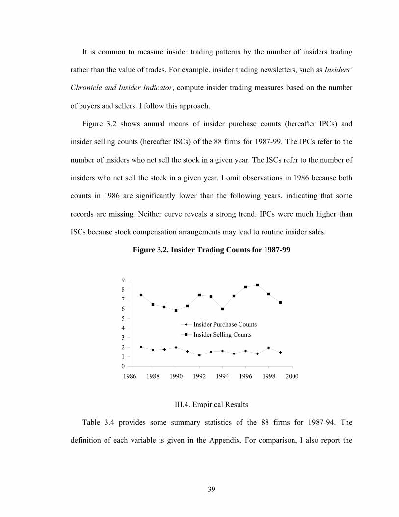
39
It is common to measure insider trading patterns by the number of insiders trading
rather than the value of trades. For example, insider trading newsletters, such as Insiders’
Chronicle and Insider Indicator, compute insider trading measures based on the number
of buyers and sellers. I follow this approach.
Figure 3.2 shows annual means of insider purchase counts (hereafter IPCs) and
insider selling counts (hereafter ISCs) of the 88 firms for 1987-99. The IPCs refer to the
number of insiders who net sell the stock in a given year. The ISCs refer to the number of
insiders who net sell the stock in a given year. I omit observations in 1986 because both
counts in 1986 are significantly lower than the following years, indicating that some
records are missing. Neither curve reveals a strong trend. IPCs were much higher than
ISCs because stock compensation arrangements may lead to routine insider sales.
Figure 3.2. Insider Trading Counts for 1987-99
0123456789
1986 1988 1990 1992 1994 1996 1998 2000
Insider Purchase CountsInsider Selling Counts
III.4. Empirical Results
Table 3.4 provides some summary statistics of the 88 firms for 1987-94. The
definition of each variable is given in the Appendix. For comparison, I also report the
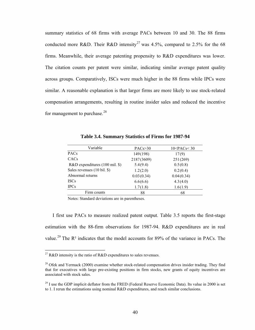
40
summary statistics of 68 firms with average PACs between 10 and 30. The 88 firms
conducted more R&D. Their R&D intensity27 was 4.5%, compared to 2.5% for the 68
firms. Meanwhile, their average patenting propensity to R&D expenditures was lower.
The citation counts per patent were similar, indicating similar average patent quality
across groups. Comparatively, ISCs were much higher in the 88 firms while IPCs were
similar. A reasonable explanation is that larger firms are more likely to use stock-related
compensation arrangements, resulting in routine insider sales and reduced the incentive
for management to purchase.28
Table 3.4. Summary Statistics of Firms for 1987-94
Variable PACs>30 10<PACs< 30 PACs 149(198) 17 (9) CACs 2187(3609) 251 (269) R&D expenditures (100 mil. $) 5.4(9.4) 0.5 (0.8)
Sales revenues (10 bil. $) 1.2(2.0) 0.2 (0.4) Abnormal returns 0.03(0.34) 0.04 (0.34) ISCs 6.6(6.6) 4.3 (4.0) IPCs 1.7(1.8) 1.6 (1.9)
Firm counts 88 68 Notes: Standard deviations are in parentheses.
I first use PACs to measure realized patent output. Table 3.5 reports the first-stage
estimation with the 88-firm observations for 1987-94. R&D expenditures are in real
value.29 The R² indicates that the model accounts for 89% of the variance in PACs. The
27 R&D intensity is the ratio of R&D expenditures to sales revenues.
28 Ofek and Yermack (2000) examine whether stock-related compensation drives insider trading. They find that for executives with large pre-existing positions in firm stocks, new grants of equity incentives are associated with stock sales.
29 I use the GDP implicit deflator from the FRED (Federal Reserve Economic Data). Its value in 2000 is set to 1. I rerun the estimations using nominal R&D expenditures, and reach similar conclusions.
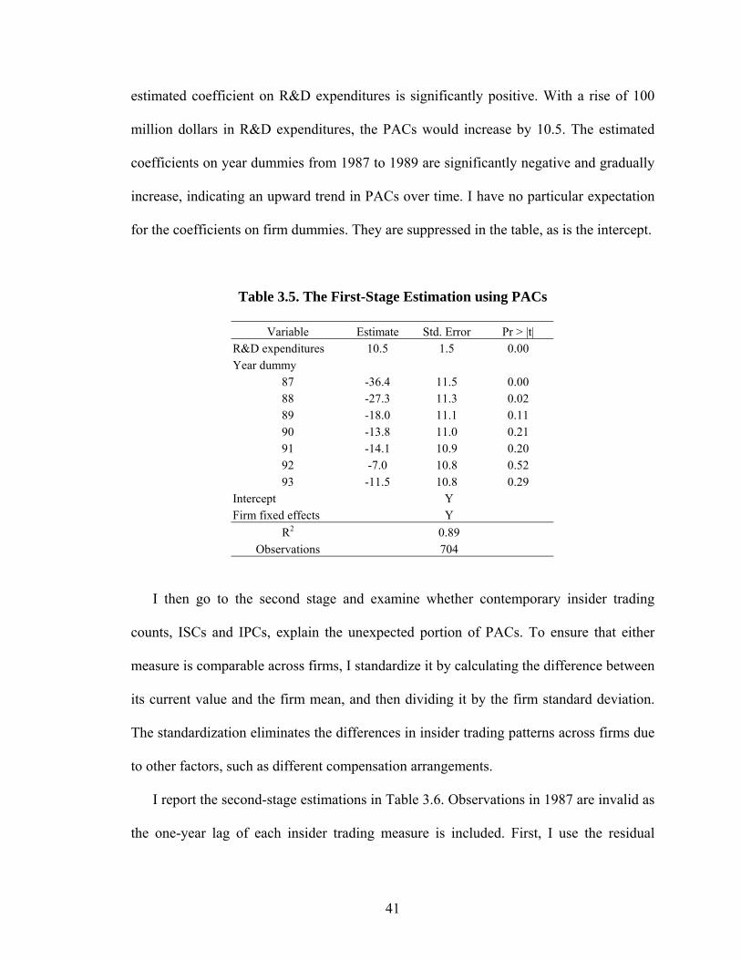
41
estimated coefficient on R&D expenditures is significantly positive. With a rise of 100
million dollars in R&D expenditures, the PACs would increase by 10.5. The estimated
coefficients on year dummies from 1987 to 1989 are significantly negative and gradually
increase, indicating an upward trend in PACs over time. I have no particular expectation
for the coefficients on firm dummies. They are suppressed in the table, as is the intercept.
Table 3.5. The First-Stage Estimation using PACs
Variable Estimate Std. Error Pr > |t| R&D expenditures 10.5 1.5 0.00 Year dummy
87 -36.4 11.5 0.00 88 -27.3 11.3 0.02 89 -18.0 11.1 0.11 90 -13.8 11.0 0.21 91 -14.1 10.9 0.20 92 -7.0 10.8 0.52 93 -11.5 10.8 0.29
Intercept Y Firm fixed effects Y
R2 0.89 Observations 704
I then go to the second stage and examine whether contemporary insider trading
counts, ISCs and IPCs, explain the unexpected portion of PACs. To ensure that either
measure is comparable across firms, I standardize it by calculating the difference between
its current value and the firm mean, and then dividing it by the firm standard deviation.
The standardization eliminates the differences in insider trading patterns across firms due
to other factors, such as different compensation arrangements.
I report the second-stage estimations in Table 3.6. Observations in 1987 are invalid as
the one-year lag of each insider trading measure is included. First, I use the residual

42
directly from the first-stage estimation. In column (2), I do not include abnormal returns.
The estimated coefficients on IPCs in each year and that on ISCs in year t+1 are
significantly different from zero with the expected sign, indicating that management
possesses timely considerable information about its patent output and trade accordingly.
The effects of ISCs are less influential than IPCs. This difference may lie in stock-related
compensations. Take stock bonuses for example. Suppose that the annual amount of
stock bonus payment is higher than what management wants to purchase. In a regular
year, we should expect routine insider sales. Management may reduce the amount of
sales when they realize the stock is underpriced. Only when the magnitude of this
underpricing is great enough would they begin to purchase. Therefore, the effects of IPCs
are more significant explanations of fluctuations of patent output than ISCs.
In column (3), I add abnormal returns to control for market effects. The estimated
coefficients on abnormal returns in year t and t+4 are significantly positive, indicating
that the unexpected portion of realized patent output is gradually reflected in stock price.
The effects of both IPCs and ISCs are persistent. For comparison, in column (1) I include
abnormal returns only. The estimation fails to pass the overall F-test at the significance
level of 10%, indicating that abnormal returns have little explanatory power on the PACs
residual. The different explanatory power between insider trading patterns and abnormal
returns further confirms that management does process timely considerable information
about its realized patent output beyond what is known to investors.
With firm dummies in the first-stage estimation, the difference in the mean PACs
across firms is eliminated from the estimated residual. Thus, the residual only reflects
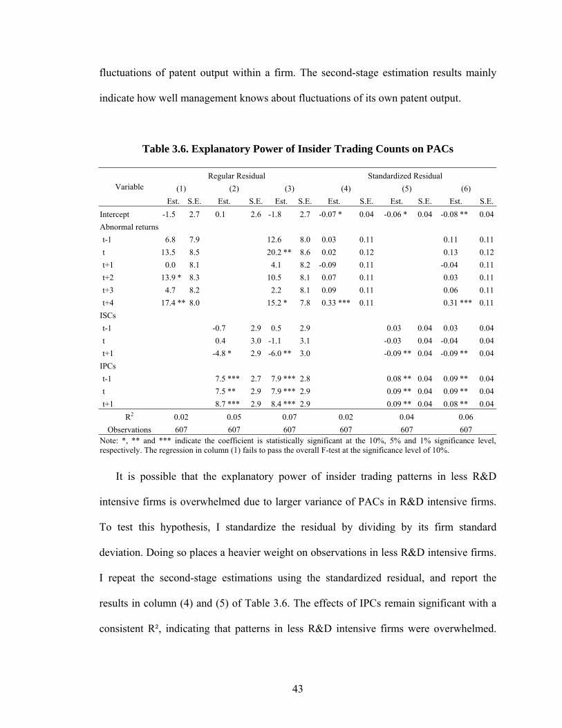
43
fluctuations of patent output within a firm. The second-stage estimation results mainly
indicate how well management knows about fluctuations of its own patent output.
Table 3.6. Explanatory Power of Insider Trading Counts on PACs
Regular Residual Standardized Residual (1) (2) (3) (4) (5) (6) Variable
Est. S.E. Est. S.E. Est. S.E. Est. S.E. Est. S.E. Est. S.E.Intercept -1.5 2.7 0.1 2.6 -1.8 2.7 -0.07 * 0.04 -0.06 * 0.04 -0.08 ** 0.04Abnormal returns t-1 6.8 7.9 12.6 8.0 0.03 0.11 0.11 0.11 t 13.5 8.5 20.2 ** 8.6 0.02 0.12 0.13 0.12 t+1 0.0 8.1 4.1 8.2 -0.09 0.11 -0.04 0.11 t+2 13.9 * 8.3 10.5 8.1 0.07 0.11 0.03 0.11 t+3 4.7 8.2 2.2 8.1 0.09 0.11 0.06 0.11 t+4 17.4 ** 8.0 15.2 * 7.8 0.33 *** 0.11 0.31 *** 0.11ISCs t-1 -0.7 2.9 0.5 2.9 0.03 0.04 0.03 0.04 t 0.4 3.0 -1.1 3.1 -0.03 0.04 -0.04 0.04 t+1 -4.8 * 2.9 -6.0 ** 3.0 -0.09 ** 0.04 -0.09 ** 0.04IPCs t-1 7.5 *** 2.7 7.9 *** 2.8 0.08 ** 0.04 0.09 ** 0.04 t 7.5 ** 2.9 7.9 *** 2.9 0.09 ** 0.04 0.09 ** 0.04 t+1 8.7 *** 2.9 8.4 *** 2.9 0.09 ** 0.04 0.08 ** 0.04
R2 0.02 0.05 0.07 0.02 0.04 0.06 Observations 607 607 607 607 607 607
Note: *, ** and *** indicate the coefficient is statistically significant at the 10%, 5% and 1% significance level, respectively. The regression in column (1) fails to pass the overall F-test at the significance level of 10%.
It is possible that the explanatory power of insider trading patterns in less R&D
intensive firms is overwhelmed due to larger variance of PACs in R&D intensive firms.
To test this hypothesis, I standardize the residual by dividing by its firm standard
deviation. Doing so places a heavier weight on observations in less R&D intensive firms.
I repeat the second-stage estimations using the standardized residual, and report the
results in column (4) and (5) of Table 3.6. The effects of IPCs remain significant with a
consistent R², indicating that patterns in less R&D intensive firms were overwhelmed.
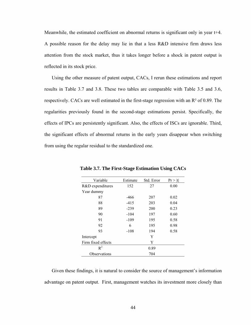
44
Meanwhile, the estimated coefficient on abnormal returns is significant only in year t+4.
A possible reason for the delay may lie in that a less R&D intensive firm draws less
attention from the stock market, thus it takes longer before a shock in patent output is
reflected in its stock price.
Using the other measure of patent output, CACs, I rerun these estimations and report
results in Table 3.7 and 3.8. These two tables are comparable with Table 3.5 and 3.6,
respectively. CACs are well estimated in the first-stage regression with an R² of 0.89. The
regularities previously found in the second-stage estimations persist. Specifically, the
effects of IPCs are persistently significant. Also, the effects of ISCs are ignorable. Third,
the significant effects of abnormal returns in the early years disappear when switching
from using the regular residual to the standardized one.
Table 3.7. The First-Stage Estimation Using CACs
Variable Estimate Std. Error Pr > |t| R&D expenditures 152 27 0.00 Year dummy
87 -466 207 0.02 88 -415 203 0.04 89 -239 200 0.23 90 -104 197 0.60 91 -109 195 0.58 92 6 195 0.98 93 -108 194 0.58
Intercept Y Firm fixed effects Y
R2 0.89 Observations 704
Given these findings, it is natural to consider the source of management’s information
advantage on patent output. First, management watches its investment more closely than
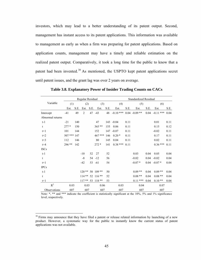
45
investors, which may lead to a better understanding of its patent output. Second,
management has instant access to its patent applications. This information was available
to management as early as when a firm was preparing for patent applications. Based on
application counts, management may have a timely and reliable estimation on the
realized patent output. Comparatively, it took a long time for the public to know that a
patent had been invented.30 As mentioned, the USPTO kept patent applications secret
until patent issues, and the grant lag was over 2 years on average.
Table 3.8. Explanatory Power of Insider Trading Counts on CACs
Regular Residual Standardized Residual (1) (2) (3) (4) (5) (6) Variable
Est. S.E. Est. S.E. Est. S.E. Est. S.E. Est. S.E. Est. S.E.Intercept -41 49 2 47 -43 48 -0.10 *** 0.04 -0.09 ** 0.04 -0.11 *** 0.04Abnormal returns t-1 -21 140 47 143 -0.04 0.11 0.01 0.11 t 277 * 150 365 ** 155 0.06 0.11 0.15 0.12 t+1 101 144 152 147 -0.07 0.11 -0.02 0.11 t+2 507 *** 147 467 *** 146 0.20 * 0.11 0.17 0.11 t+3 112 146 80 145 0.04 0.11 0.02 0.11 t+4 296 ** 142 272 * 141 0.38 *** 0.11 0.36 *** 0.11ISCs t-1 -10 52 27 52 0.03 0.04 0.05 0.04 t -8 54 -12 56 -0.02 0.04 -0.02 0.04 t+1 -42 53 -61 54 -0.07 * 0.04 -0.07 * 0.04IPCs t-1 120 ** 50 109 ** 50 0.09 ** 0.04 0.09 ** 0.04 t 114 ** 52 116 ** 52 0.08 ** 0.04 0.08 ** 0.04 t+1 117 ** 53 118 ** 53 0.11 *** 0.04 0.10 ** 0.04
R2 0.03 0.03 0.06 0.03 0.04 0.07 Observations 607 607 607 607 607 607
Note: *, ** and *** indicate the coefficient is statistically significant at the 10%, 5% and 1% significance level, respectively.
30 Firms may announce that they have filed a patent or release related information by launching of a new product. However, a systematic way for the public to instantly know the current status of patent applications was not available.
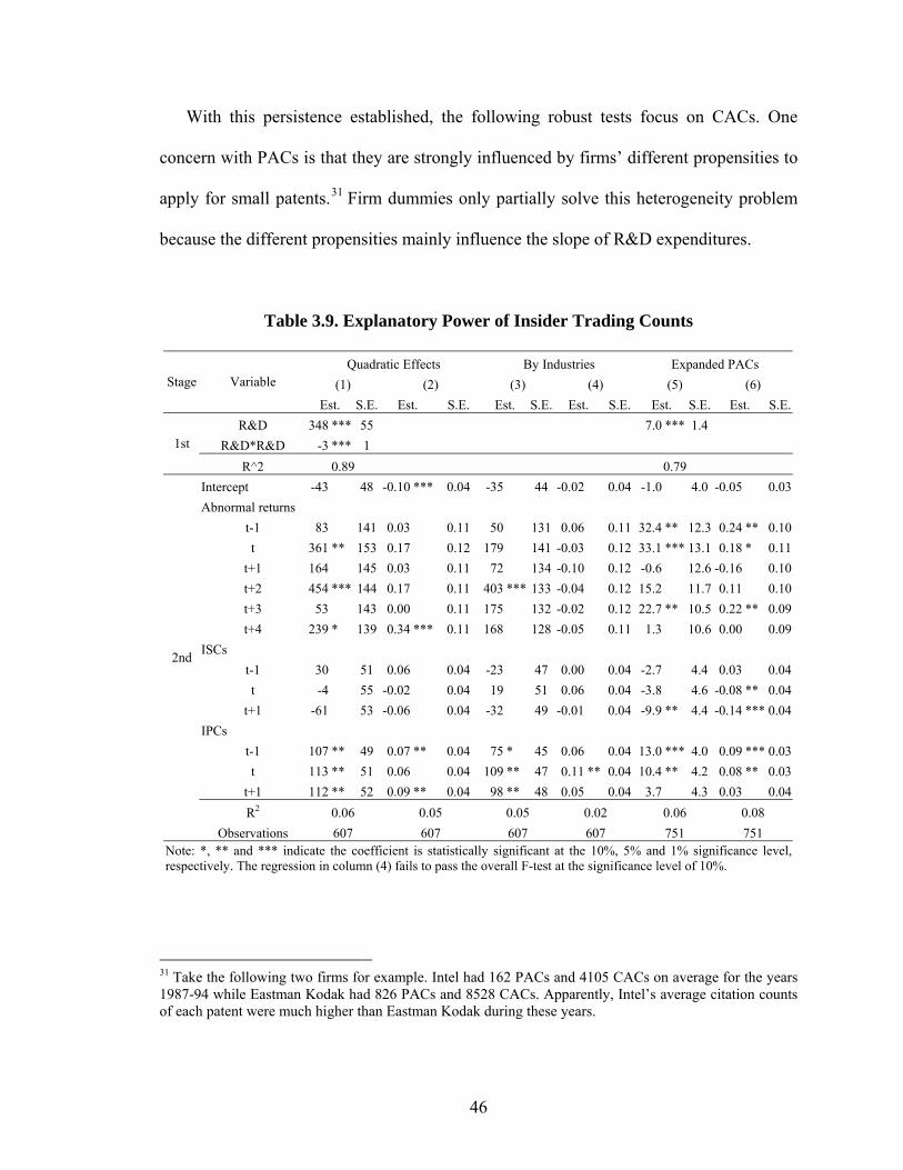
46
With this persistence established, the following robust tests focus on CACs. One
concern with PACs is that they are strongly influenced by firms’ different propensities to
apply for small patents.31 Firm dummies only partially solve this heterogeneity problem
because the different propensities mainly influence the slope of R&D expenditures.
Table 3.9. Explanatory Power of Insider Trading Counts
Quadratic Effects By Industries Expanded PACs (1) (2) (3) (4) (5) (6) Stage Variable
Est. S.E. Est. S.E. Est. S.E. Est. S.E. Est. S.E. Est. S.E.R&D 348 *** 55 7.0 *** 1.4
R&D*R&D -3 *** 1 1st
R^2 0.89 0.79 Intercept -43 48 -0.10 *** 0.04 -35 44 -0.02 0.04 -1.0 4.0 -0.05 0.03Abnormal returns
t-1 83 141 0.03 0.11 50 131 0.06 0.11 32.4 ** 12.3 0.24 ** 0.10t 361 ** 153 0.17 0.12 179 141 -0.03 0.12 33.1 *** 13.1 0.18 * 0.11
t+1 164 145 0.03 0.11 72 134 -0.10 0.12 -0.6 12.6 -0.16 0.10t+2 454 *** 144 0.17 0.11 403 *** 133 -0.04 0.12 15.2 11.7 0.11 0.10t+3 53 143 0.00 0.11 175 132 -0.02 0.12 22.7 ** 10.5 0.22 ** 0.09t+4 239 * 139 0.34 *** 0.11 168 128 -0.05 0.11 1.3 10.6 0.00 0.09
ISCs t-1 30 51 0.06 0.04 -23 47 0.00 0.04 -2.7 4.4 0.03 0.04t -4 55 -0.02 0.04 19 51 0.06 0.04 -3.8 4.6 -0.08 ** 0.04
t+1 -61 53 -0.06 0.04 -32 49 -0.01 0.04 -9.9 ** 4.4 -0.14 *** 0.04IPCs
t-1 107 ** 49 0.07 ** 0.04 75 * 45 0.06 0.04 13.0 *** 4.0 0.09 *** 0.03t 113 ** 51 0.06 0.04 109 ** 47 0.11 ** 0.04 10.4 ** 4.2 0.08 ** 0.03
t+1 112 ** 52 0.09 ** 0.04 98 ** 48 0.05 0.04 3.7 4.3 0.03 0.04R2 0.06 0.05 0.05 0.02 0.06 0.08
2nd
Observations 607 607 607 607 751 751 Note: *, ** and *** indicate the coefficient is statistically significant at the 10%, 5% and 1% significance level,respectively. The regression in column (4) fails to pass the overall F-test at the significance level of 10%.
31 Take the following two firms for example. Intel had 162 PACs and 4105 CACs on average for the years 1987-94 while Eastman Kodak had 826 PACs and 8528 CACs. Apparently, Intel’s average citation counts of each patent were much higher than Eastman Kodak during these years.
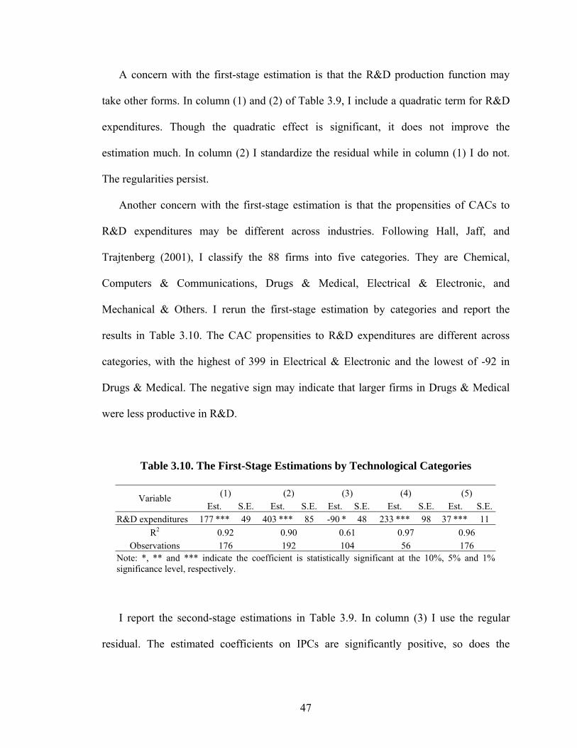
47
A concern with the first-stage estimation is that the R&D production function may
take other forms. In column (1) and (2) of Table 3.9, I include a quadratic term for R&D
expenditures. Though the quadratic effect is significant, it does not improve the
estimation much. In column (2) I standardize the residual while in column (1) I do not.
The regularities persist.
Another concern with the first-stage estimation is that the propensities of CACs to
R&D expenditures may be different across industries. Following Hall, Jaff, and
Trajtenberg (2001), I classify the 88 firms into five categories. They are Chemical,
Computers & Communications, Drugs & Medical, Electrical & Electronic, and
Mechanical & Others. I rerun the first-stage estimation by categories and report the
results in Table 3.10. The CAC propensities to R&D expenditures are different across
categories, with the highest of 399 in Electrical & Electronic and the lowest of -92 in
Drugs & Medical. The negative sign may indicate that larger firms in Drugs & Medical
were less productive in R&D.
Table 3.10. The First-Stage Estimations by Technological Categories
(1) (2) (3) (4) (5) Variable Est. S.E. Est. S.E. Est. S.E. Est. S.E. Est. S.E.
R&D expenditures 177 *** 49 403 *** 85 -90 * 48 233 *** 98 37 *** 11 R2 0.92 0.90 0.61 0.97 0.96
Observations 176 192 104 56 176 Note: *, ** and *** indicate the coefficient is statistically significant at the 10%, 5% and 1% significance level, respectively.
I report the second-stage estimations in Table 3.9. In column (3) I use the regular
residual. The estimated coefficients on IPCs are significantly positive, so does the

48
coefficient on abnormal returns in year t+2. In column (4) I use the standardized residual.
The estimation fails to pass the overall F-test at the significance level of 10%. However,
it passes the test when abnormal returns are excluded. To verify that the significance of
insider trading effects does not come from the poor estimation in Drugs & Medical firms,
I exclude these firms, and reach similar estimation results.
I manage to extend the patent granting record up to 2002 based on the updated patent
file in Bronwyn Hall’s website. I repeat the estimations in Table 3.5 and 3.6 with
observations of two more years, and report the results briefly in column (5) and (6) of
Table 3.9. The estimated PAC propensity to R&D expenditures drops significantly from
7.7 to 5.2 with these additional observations. In column (6) I standardize the residual
while in column (5) I do not. In either case, the estimated coefficients on IPCs remain
significant but only for year t-1 and t, indicating management’s prompt reactions to
patent output after 1994. It is interesting to see that market reactions also happened
earlier. It is hard to explain why the effects of ISCs become more influential. Again, the
R² increases significantly when I switch to using the standardized residual.
To double check how the explanatory power of insider trading patterns is influenced
by firms’ R&D intensity, I divide the 88 firms into two groups based on the mean PACs,
with the highest 44 firms in one group and the lowest 44 firms in the other. I rerun the
estimations for each group, and report the results in Table 3.11. The estimated
coefficients on IPCs are significantly postive in the highest 44 firms but not in the lowest
44 firms. Therefore, I conclude that it is more likely to detect the explanatory power of
IPCs in R&D intensive firms. In the estimations of the highest 44 firms, the R² increases
significantly from 0.09 to 0.14 when switching from using the regular residual to the
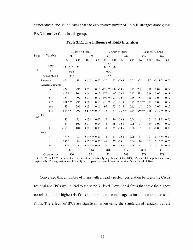
49
standardized one. It indicates that the explanatory power of IPCs is stronger among less
R&D intensive firms in this group.
Table 3.11. The Influence of R&D Intensities
Highest 44 firms Lowest 44 firms Highest 40 firms (1) (2) (3) (4) (5) (6) Stage Variable
Est. S.E. Est. S.E. Est. S.E. Est. S.E. Est. S.E. Est. S.E.
R&D 130 *** 39 300*** 80
R2 0.88 0.59 1st
Observations 352 352 Intercept -76 89 -0.11 ** 0.05 -25 33 -0.08 0.05 -83 97 -0.11 ** 0.05Abnormal returns
t-1 227 296 0.05 0.16 -178 ** 90 -0.06 0.15 238 310 0.07 0.17t 612 ** 304 0.16 0.17 179 * 102 0.08 0.17 532 * 319 0.09 0.18
t+1 126 297 0.01 0.17 197 ** 93 -0.01 0.15 157 310 0.00 0.17t+2 801 *** 296 0.16 0.16 230 ** 92 0.18 0.15 707 ** 312 0.09 0.17t+3 52 290 -0.13 0.16 95 93 0.14 0.15 167 306 -0.09 0.17t+4 668 ** 297 0.43 *** 0.16 -3 87 0.27 * 0.14 659 ** 316 0.42 ** 0.17
ISCs t-1 50 95 0.13 ** 0.05 19 36 -0.03 0.06 3 104 0.11 ** 0.06t 24 109 0.01 0.06 -11 36 -0.05 0.06 -24 119 -0.02 0.07
t+1 -156 104 -0.08 0.06 -1 35 -0.05 0.06 -152 112 -0.08 0.06IPCs
t-1 170 * 93 0.14 *** 0.05 1 34 0.00 0.06 156 101 0.14 ** 0.06t 186 * 94 0.17 *** 0.05 49 37 -0.01 0.06 116 101 0.13 ** 0.06
t+1 169 * 96 0.15 *** 0.05 24 36 0.03 0.06 154 103 0.14 ** 0.06R2 0.10 0.14 0.08 0.04 0.08 0.11
2nd
Observations 306 306 301 301 278 278 Note: *, ** and *** indicate the coefficient is statistically significant at the 10%, 5% and 1% significance level, respectively. The regression in column (4) fails to pass the overall F-test at the significance level of 10%.
Concerned that a number of firms with a nearly perfect correlation between the CACs
residual and IPCs would lead to the same R² level, I exclude 4 firms that have the highest
correlation in the highest 44 firms and rerun the second-stage estimations with the rest 40
firms. The effects of IPCs are significant when using the standardized residual, but are
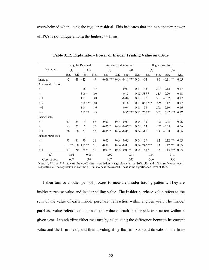
50
overwhelmed when using the regular residual. This indicates that the explanatory power
of IPCs is not unique among the highest 44 firms.
Table 3.12. Explanatory Power of Insider Trading Value on CACs
Regular Residual Standardized Residual Highest 44 firms (1) (2) (3) (4) (5) (6) Variable
Est. S.E. Est. S.E. Est. S.E. Est. S.E. Est. S.E. Est. S.E.Intercept -2 48 -42 49 -0.09 *** 0.04 -0.11 *** 0.04 -64 90 -0.11 ** 0.05Abnormal returns t-1 -18 147 0.01 0.11 135 307 0.12 0.17 t 306 * 160 0.13 0.12 587 * 315 0.20 0.18 t+1 117 148 -0.06 0.11 90 301 -0.02 0.17 t+2 518 *** 148 0.18 0.11 858 *** 299 0.17 0.17 t+3 114 146 0.04 0.11 56 292 -0.10 0.16 t+4 313 ** 143 0.37 *** 0.11 766 ** 302 0.47 *** 0.17Insider sales t-1 -43 54 9 56 -0.02 0.04 0.01 0.04 33 102 0.05 0.06 t -5 53 7 56 -0.07 * 0.04 -0.07 * 0.04 33 107 -0.08 0.06 t+1 20 50 23 52 -0.06 * 0.04 -0.05 0.04 -15 99 -0.08 0.06Insider purchases t-1 78 51 70 51 0.05 0.04 0.05 0.04 129 92 0.12 ** 0.05 t 103 ** 50 115 ** 50 -0.01 0.04 -0.01 0.04 242 *** 93 0.12 ** 0.05 t+1 73 50 84 * 50 0.07 * 0.04 0.07 * 0.04 163 * 92 0.15 *** 0.05
R2 0.01 0.05 0.02 0.04 0.09 0.11 Observations 607 607 607 607 306 306
Note: *, ** and *** indicate the coefficient is statistically significant at the 10%, 5% and 1% significance level, respectively. The regression in column (1) fails to pass the overall F-test at the significance level of 10%.
I then turn to another pair of proxies to measure insider trading patterns. They are
insider purchase value and insider selling value. The insider purchase value refers to the
sum of the value of each insider purchase transaction within a given year. The insider
purchase value refers to the sum of the value of each insider sale transaction within a
given year. I standardize either measure by calculating the difference between its current
value and the firm mean, and then dividing it by the firm standard deviation. The first-

51
stage estimation remains the same as in Table 3.7. The second-stage estimations are
reported in Table 3.12. In column (1) and (3) the estimations without control for
abnormal returns fail to pass the overall F-test at the significance level of 10%.
In column (5) and (6) I only include the highest 44 firms. The estimated coefficient
on IPCs turn to be significant while the R2 of the regression using the standardized
residual is lower than that in column (2) of Table 3.11. It indicates that the explanatory
power of insider trading patterns on patent output is stronger when using the number of
insiders trading instead of insider trading values as the measure. This finding is consistent
with the business convention of using the number of insiders engaged in trading. The
reason may lie in that good news becomes less reliable when it is spread from top
management to ordinary managers. When an ordinary manager, whose income is not
comparable to top management, makes a relatively small purchase based on this less
reliable information, it should add more credit to the significance of the good news than
what is reflected by his purchase value.
III.5. Conclusions
My purpose of this chapter is to identify how informative insider trading patterns are
in predicting a firm’s patent output. By examining R&D intensive firms, I found strong
evidence that the effects of contemporary insider trading patterns are significant to
explain fluctuations of patent output when controlling for market effects, as well as R&D
input effects. The findings are consistent across different measures of patent output,
across different time scales, and across different measures of insider trading patterns.
Therefore, I concluded that management has timely and privileged information about its

52
realized patent output beyond what is known to investors. I also found that the
explanatory power of insider trading patterns on patent output comes from purchases
rather than sales.
In business practice, comparing patent output between firms may help to evaluate
which firm stands a better chance to beat the market. My findings suggest that, to obtain a
timely estimate of a firm’s realized patent output, it is worth to take IPCs into account.
Moreover, this approach is more effective in R&D intensive firms. My further study
would be to investigate whether the explanatory power of insider trading patterns on
patent output is consistent over time at the firm level; and if so, what factors would
explain the consistency.
In this study I do not join the debate on the social consequence of insider trading.
However, for those concerned with this issue, my results point to an important source of
private information - patent output. Improved disclosure on its relevant information, such
as patent applications, may be considered as means for reducing information asymmetry.
Doing so would make investors better informed of a firm’s R&D performance. Since
document preparation takes time, management would still have early access to
application information. Thus, management would not have much incentive to change the
pattern of patent applications when this disclosure is required.
53
References
Aboody, D., and B. Lev (2000): “Information Asymmetry, R&D, and Insider Gains.” Journal of Finance 55(6):2747-2766.
Albert, M. B., D. Avery, F. Narin, and P. McAllister (1991): “Direct Validation of Citation Counts as Indicators of Industrially Important Patents.” Research Policy 20:251-259.
Barth, M., R. Kasznik, and M. McNichols (2001): “Analyst Coverage and Intangible Assets.” Journal of Accounting Research 39(1):1-34.
Bettis, C., D. Vickrey, and D. W. Vickrey (1997): “Mimickers of Corporate Insiders Who Make large Volume Trades.” Financial Analysts Journal 53:57-66.
Deng, Z., B. Lev, and F. Narin (1999): “Science and Technology as Predictors of Stock Performance.” Financial Analysts Journal 55:20-32.
Earnst, H. (1999): “Evaluation of Dynamic Technological Developments by Means of Patent Data.” The Dynamics of Innovation: Strategic and Managerial Implications. K. Brochhoff, A. K. Chakrabarti, and J. Hauschildt ed. Springer, Berlin.
Finnerty, J. E. (1976): “Insiders and Market Efficiency.” Journal of Finance 31(4):1141-1148.
Griliches, Z. (1995): “R&D and Productivity: Econometric Results and Measurement Issues.” Handbook of the Economics of Innovation and Technological Change. Paul Stoneman ed. Blackwell, Oxford.
Hall, B. H., A. B. Jaffe and M. Trajtenberg (2001): “The NBER Patent Citation Data File: Lessons, Insights and Methodological Tools.” National Bureau of Economic Research Working Paper No. 8498.
Hall, B. H., A. B. Jaffe and M. Trajtenberg (2005): “Market Value and Patent Citations.” RAND Journal of Economics 36(1):16-38.
Hall, B. H., Z. Griliches, and J. A. Hausman (1986): “Patents and R and D: Is There a Lag?” International Economic Review 27(2):265-283.
Jaffe, J. (1974): “Special Information and Insider Trading.” Journal of Business 47:410-428.
Jeng, L., A. Metrick, and R. Zeckhauser (2003): “Estimating the Returns to Insider Trading: A Performance-Evaluation Perspective.” Review of Economics and Statistics 85(2):453-471.

54
John, K., and L. Lang (1991): “Strategic Insider Trading around Dividend Announcements: Theory and Evidence.” Journal of Finance 46:1361--1398.
Karpoff, J. M., and D. Lee (1991): “Insider Trading before New Issue Announcements.” Financial Management 20:18--26.
Kothari, S. P., T. Laguerre, and A. Leone (2002): “Capitalization versus Expensing: Evidence on the Uncertainty of Future Earnings from Capital Expenditures versus R&D Outlays.” Review of Accounting Studies 7:355-382.
Lee, D. S., W. H. Mikkelson, and M. M. Partch (1992): “Managers’ Trading around Stock Repurchases.” Journal of Finance 47:1947-1961.
Lakonishok, J., and I. Lee (2001): “Are Insider Trades Informative?” Review of Financial Studies 14: 79-111.
Ofek, E., and D. Yermack, (2000): “Taking Stock: Equity-Based Compensation and the Evolution of Managerial Ownership.” Journal of Finance 55:1367-1384.
Pakes, A., and Z. Griliches (1980): “Patents and R&D at the Firm Level: A First Report.” Economics Letters 5:377-381.
Romer, C. D., and D. H. Romer (2000): “Federal Reserve Information and the Behavior of Interest Rates.” American Economic Review 90(3):429-457.
Rozeff, M. S., and M. A. Zaman (1988): “Market Efficiency and Insider Trading: New Evidence.” Journal of Business 61:25-44.
Scherer, F. M. (1965): “Firm Size, Market Structure, Opportunity, and the Output of Patented Innovations.” American Economic Review 55:1097-1123.
Schmookler, J. (1966): Invention and Economic Growth. Cambridge: Harvard University Press.
Seyhun, N. (1986): “Insiders’ Profits, Costs of Trading, and Market Efficiency.” Journal of Financial Economics 16:198-212.
Seyhun, N. (1990): “Do Bidder Managers Knowingly Pay Too Much for Target Firms?” Journal of Business 63:439-464.
Seyhun, N. and M. Bradley (1997): “Corporate Bankruptcy and Insider Trading.” Journal of Business 70:189-216.
Tasker, S. (1998): “Technology Company Conference Calls: A Small Sample Study.” Journal of Financial Statement Analysis 4:6-14.

55
Appendix
Variable Description
The specific variables used in the analysis are defined as follows:
. Patent Annual Counts (PACs) is defined as the number of granted patents that are applied for in a given year.
. Citation Annual Counts (CACs) is defined as the summed citation counts of those granted patents that are applied for in a given year. Here, citation counts of a patent are the number of citations that the patent received until August 2006.
. R&D Expenditures is R&D expenditures (Compustat item 46) in the fiscal year.
. Sales Revenues is sales revenues (Compustat item 12) in the fiscal year.
. Abnormal Return equals the stock annual return minus the S&P Industrial Index annual return.
. Insider Selling Counts (ISCs) is the number of insiders who net sell the stock in a given year.
. Insider Purchase Counts (IPCs) the number of insiders who net buy the stock in a given year.
. Insider Selling Value is the sum of the value of each insider sale transaction within a given year. The value of an insider sale transaction equals the transaction volume times the transaction price.
. Insider Purchase Value is the sum of the value of each insider purchase transaction within a given year. The value of an insider purchase transaction equals the transaction volume times the transaction price.

56
A List of the 88 Firms by Categories
Chemical Computers & Communications AIR PRODUCTS & CHEMICALS AT&T CORP AMOCO CORP ADVANCED MICRO DEVICES ATLANTIC RICHFIELD CO AMP INC BETZDEARBORN INC APPLE COMPUTER INC COLGATE-PALMOLIVE CO COMPAQ COMPUTER CORP DOW CHEMICAL CORNING INC DRESSER INDUSTRIES INC DIGITAL EQUIPMENT DU PONT (E I) DE NEMOURS GTE CORP FMC CORP HARRIS CORP GOODYEAR TIRE & RUBBER C HEWLETT-PACKARD CO HERCULES INC HONEYWELL INC INTL PAPER CO INTEL CORP KIMBERLY-CLARK CORP INTL BUSINESS MACHINES C LUBRIZOL CORP MICRON TECHNOLOGY INC MEAD CORP MOLEX INC NALCO CHEMICAL CO MOTOROLA INC PPG INDUSTRIES INC NATIONAL SEMICONDUCTOR C PROCTER & GAMBLE CO RAYTHEON CO ROHM AND HAAS CO SEAGATE TECHNOLOGY-OLD SCHLUMBERGER LTD SUN MICROSYSTEMS INC TEXACO INC TEXAS INSTRUMENTS INC UNION CARBIDE CORP UNISYS CORP VLSI TECHNOLOGY INC Drugs & Medical XEROX CORP ABBOTT LABORATORIES ALZA CORP Mechanical & Others BAXTER INTERNATIONAL INC BAKER HUGHES INC BECTON DICKINSON & CO BOEING CO BRISTOL-MYERS SQUIBB CO BRUNSWICK CORP JOHNSON & JOHNSON CATERPILLAR INC LILLY (ELI) & CO CHRYSLER CORP MEDTRONIC INC DANA CORP MERCK & CO DEERE & CO PFIZER INC EATON CORP SCHERING-PLOUGH FORD MOTOR CO U S SURGICAL CORP GENERAL MOTORS CORP WARNER-LAMBERT CO GOODRICH CORP HALLIBURTON CO Electrical & Electronics ILLINOIS TOOL WORKS EASTMAN KODAK CO LITTON INDUSTRIES INC EMERSON ELECTRIC CO MCDONNELL DOUGLAS CORP GENERAL ELECTRIC CO OLIN CORP RAYCHEM CORP OUTBOARD MARINE CORP TEKTRONIX INC PITNEY BOWES INC WHIRLPOOL CORP SUNDSTRAND CORP ZENITH ELECTRONICS CORP TRW INC TEXTRON INC UNITED TECHNOLOGIES CORP
57
IV. HOW DO KNOWLEDGE STOCKS INFLUENCE THE START-UP AND
SURVIVAL OF NEW MANUFACTURING SEGMENTS IN U.S. PATENTING
FIRMS?
IV.1. Introduction
Penrose (1959) explains how investment in research and development (R&D) can
induce later diversification.32 The reasoning is that the output of R&D is new knowledge,
and markets for exchanging new knowledge are subject to well-known problems.33 This
makes market exchange relatively costly for appropriating returns to new knowledge. As
a result, firms often diversify into the new industry in order to more fully appropriate
these returns.
Conversely, diversification may stimulate research activities. The idea - first explored
by Nelson (1959) - is as follows. Research is an uncertain activity, resulting in inventions
in unexpected areas. A diversified firm is more likely to be able to produce and market
these unexpected inventions than a firm characterized by a narrow product line.
Therefore, more diversified firms would expect a higher profit from research. And this, in
turn, leads the firm to support more research. Inspired by this theory, subsequent studies
have shown that there is a positive relation between diversification and R&D intensity.34
32 R&D is not the only reason for new industry entry. Supply relationships or marketing similarities may also induce diversification (Williamson (1979); Penrose (1959)). Montgomery (1994) provides an excellent summary.
33 Teece (1980) first points out that the new knowledge Penrose describes has no implication for new industry entry unless the external exchange is subject to market failure.
34 Using patent counts as a measure of a firm’s knowledge intensity, Scherer (1983) finds that diversified firms patent more than other firms. Controlling for scale, Grabowski (1968) shows that firms’ R&D-to-sales ratios are positively related to how diversified the firms are in the chemical and drug industries but

58
With these diversification effects, it becomes unclear how new knowledge influences
ensuing industry entry. Diversification stimulates R&D activities and generates more
knowledge. However, this newly acquired knowledge is more likely to be absorbed
within the currently existing lines of business that the firm is operating, and thus is less
likely to take the form of new industry entry. It is an empirical question how knowledge
accumulation influences new industry entry in the presence of diversification effects.
Unfortunately, few clues to the solution can be found in the literature. Empirical
studies mostly concentrate on diversification at a point in time (e.g., Gollop and Monahan
(1991); Baldwin and Gu (2005)). They fail to identify the relationship between
innovation and firm dynamics, specifically here new industry entry. Among the few
exceptions are Gort (1969), who finds that firms with high proportions of technical
personnel have a greater tendency to merge. Further, MacDonald (1985) and Hall (1988)
both find that high R&D firms tend to enter other high R&D industries.
By examining U.S. public patenting firms35 in manufacturing sectors for 1985-96, I
find that cumulative patent counts, as a measure of knowledge stocks, predict the
likelihood of new market entry. This predictive power is weakened when diversification
effects are taken into account. Moreover, these diversification effects are significantly
positive in predicting entry likelihood. What I find is consistent with a refined version of
Nelson’s theory: knowledge stocks stimulate R&D productivity; the effect of absorbing
not in the oil industry. Gort (1962) shows that more diversified firms employ relatively more complex technology. Other empirical studies that relate diversification and innovation at the firm level are based on technological diversification measures (e.g., Audretsch and Feldman (1999)).
35 A patenting firm is defined as having at least one patent registered by the USPTO (United States Patent and Trademark Office) before 1985. See more details in Section IV.3.

59
new knowledge within lines of business does not dominate; and the appropriation still
takes the form of new industry entry.
Knowledge stocks may also influence subsequent diversification of a firm by
enhancing the survival likelihood of the newly established business. How firm
characteristics influence plant survival is an active area of empirical research. Studies on
plant deaths in declining industries confirm that larger plants are less likely to exit (e.g.,
Dunne, Robert, and Samuelson (1989a)). Studies on a wide range of industries generally
report lower death rates for plants in multi-product firms (e.g., Dunne, Robert, and
Samuelson (1989b); Disney, Haskel, and Heden (2003)).36 However, after controlling for
plant and industry characteristics, Bernard and Jensen (2007) find that plants are more
likely to close in multi-product firms or in U.S. multinationals.37
My survival study of newly established segments in patenting firms shows that initial
knowledge stocks have a significantly positive influence on segment survival, and the
influence fades over time. In contrast with traditional findings in plant survival studies, I
find that neither initial segment size, initial firm size, nor the degree of diversification
shows any significant effect. This insignificance persists when I include all
manufacturing firms in my sample. Doing so also removes the significance of knowledge
effects.
36 In fact, the finding of Disney, Haskel, and Heden (2003) is undetermined. The result is reversed when conditioned on the average characteristics. Single establishments with average group characteristics have a lower hazard than group establishments with the characteristics of singles.
37 They suggest that the ability to enter and exit flexibly may be itself a capability of firms. See also Sutton (2005).

60
This chapter is organized as follows. In Section IV.2, I present a dynamic model of a
firm’s entry and exit along with a description of its implications. Section IV.3 describes
the data used and Section IV.4 reports empirical results. Section IV.5 concludes.
IV.2. A Simple Model
The following dynamic model of a firm’s entry and exit in different product lines is a
modification of the model developed by Klette and Kortum (2004). A firm produces a
portfolio of products. Each product is provided by only one firm and yields an equalized
profit 0 1π< < .38 A firm with n products receives profit rate nπ . Further, the firm is
characterized by an independent Poisson process of becoming either a firm with 1n −
products or 1n + products. By investing in innovation, the firm influences both hazard
rates. A firm with n products chooses an innovation policy ( ) ( )( )1 2,I n I n to maximize
its expected present value, ( )V n , given an interest rate r. A firm with 0n = exits
permanently, so (0) 0V = . The corresponding Bellman equation is
( ) ( )1 2
21 1 2 1 1 2 2,
( ) max ( , ) ( ) ( 1) ( 1)I I
IrV n n C I n nc I n V n n I V nn
π γ γ⎧ ⎫= − − + + Δ + + − Δ −⎨ ⎬⎩ ⎭
(4.1)
where ( ) ( ) ( 1)V n V n V nΔ ≡ − − , and the Poisson hazard rate of losing a product equals 0
if 2 2I nγ> . When 2 0I = and 1 0γ = , equation (4.1) collapses to the Klette and Kortum
(2004) model.
38 An interpretation of such a market structure is the quality ladder model of Grossman and Helpman (1991). Innovations take the form of quality improvements. The innovator with the highest quality for a particular good captures the entire market.

61
A firm may employ resources in innovation in order to increase 1I , as a result of
which the Poisson hazard rate of acquiring a good would increase. The innovation
productivity is enhanced by the firm’s cumulative knowledge stocks. These stocks are
properly indexed by the number of product lines in which it is currently operating. The
degree of diversification, which is also indexed by product scope n, is supposed to
influence the entry hazard. This influence is measured by the rate 1γ . This parameter
reflects the first-order effect of diversification. Given an innovation for a particular good,
the firm would successfully beat the incumbent and take over the market.
Meanwhile, a firm faces the possibility that some other firm will innovate a good it is
producing. Should this happen, the firm will lose that good from its portfolio. The
Poisson hazard rate of this occurring for a particular product is 2 0γ > . With the
assumption of symmetry, the effort put forth to prevent losing any operating product
should be equalized. Thus, a firm with n products would put forth an equalized
innovative effort to determine 2 /I n by which the hazard rate of losing a particular
product would decrease.
In the above Bellman, I assumed that the production processes of 1I and 2 /I n are
divisible. I assume further that the production of 1I follows constant returns to scale with
respect to the knowledge stocks n. Therefore,
1 11 1 1 1( , ) ( ,1) ( )I IC I n nC nc
n n= = (4.2)
Both unit cost functions, 1c and 2c , are well behaved.39
39 That is ( )0 0c = , ( )c x is twice differentiable, and strictly convex for 0x ≥ .

62
Under these assumptions, equation (4.1) yields the following first-order conditions:
11' ( ) ( 1)Ic V n
n= Δ + (4.3)
22' ( ) ( )Ic V n
n= Δ . (4.4)
It is easy to verify that the solution to (4.1) is
1 1
2 2
( ) ,( ) ,( ) ,
V n vnI n nI n n
λλ
===
(4.5)
where 1λ , 2λ , and v are constants and solve40
( ) ( )
1 1 2 2
1 1 2 2 1 2 1 2
' ( ) ' ( ) ,( ) ( ) .
c c vrv c c v v
λ λπ λ λ λ λ γ γ= =
= − − + + + − (4.6)
I refer to the term 1 1( ) /I n nλ = as the firm’s external innovation intensity, and
2 2 ( ) /I n nλ = to be the firm’s internal innovation intensity. Both are independent of firm
size since both production functions are homogeneous of degree one with respect to n. It
turns out that the value of entering a product line and the value of preventing the loss of
one are identical, so the firm would distribute its R&D resources such that the marginal
cost of innovation to favor its expansion in each area is equalized. This is what is shown
in (4.6). The solution to (4.6) is unique. Furthermore, both innovation intensities are
40 I exclude the possibility of corner solutions by assuming that it is always better off to invest in both innovations, and that investing all the profit in innovations is not optimal. I also assume that it is too expensive for 2 /I n to reach its upper bound 2γ . See the proof in the Appendix for details.

63
increasing in π and 2γ . They are decreasing in 1γ , r, and an upward shift of marginal
cost 'c . See the Appendix for the proof.
We can now characterize the dynamic process for an individual firm. Consider a firm
with n products. At any given time it will remain in its current state, acquire a product
and grow to 1n + , or lose a product and shrink to 1n − . The firm that is likely to become
more diversified has a hazard rate of acquiring a product greater than that of losing one.41
In my setting, the hazard rate of acquiring a product (given product scope n) at period
T is
1 1 1 1( 1| , )HR n n T I n n nγ λ γ+ = + = + . (4.7)
The first term indicates that the likelihood of entry is positively related to knowledge
stocks when they enhance the productivity of external innovations. The second term
captures the diversification effect. Following Nelson (1959), 1γ is positive. This effect
may not be detectable when new entry occurs within current lines of business. Moreover,
my model indicates an identification problem between the knowledge effect and the
diversification effect because of their linear correlation.
The hazard of losing a product at period T is
( )2 2 2 2( 1| , )HR n n T n I nγ γ λ− = − = − . (4.8)
41 Klepper and Thompson (2006) obtain a similar result at the submarket level. They construct a model of industry evolution in which the central force for change is the creation and destruction of submarkets. A firm expands when it is able to exploit new opportunities that arrive in the form of submarkets; it contracts when its submarkets are destroyed. They prove that the number of submarkets it is involved in, which is a good measure of diversification, in the stationary state is θλμ , where θ is the mean entry rate and λμ is the mean active life of submarkets.
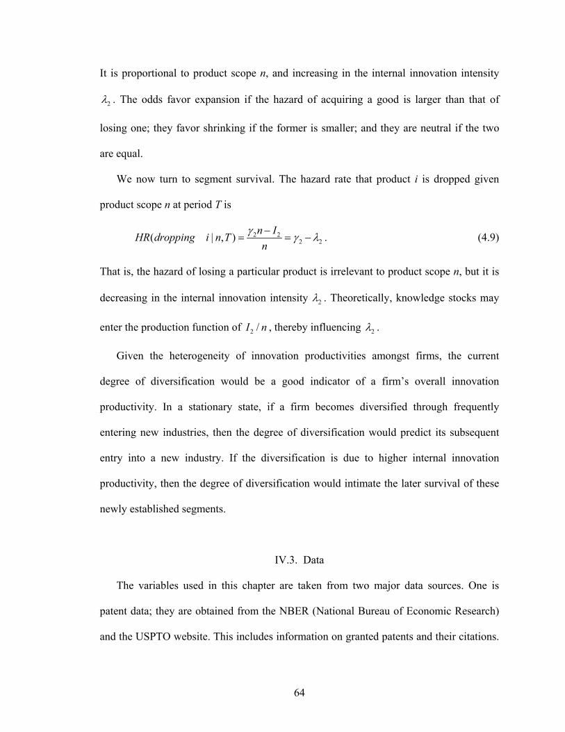
64
It is proportional to product scope n, and increasing in the internal innovation intensity
2λ . The odds favor expansion if the hazard of acquiring a good is larger than that of
losing one; they favor shrinking if the former is smaller; and they are neutral if the two
are equal.
We now turn to segment survival. The hazard rate that product i is dropped given
product scope n at period T is
2 22 2( | , ) n IHR dropping i n T
nγ γ λ−
= = − . (4.9)
That is, the hazard of losing a particular product is irrelevant to product scope n, but it is
decreasing in the internal innovation intensity 2λ . Theoretically, knowledge stocks may
enter the production function of 2 /I n , thereby influencing 2λ .
Given the heterogeneity of innovation productivities amongst firms, the current
degree of diversification would be a good indicator of a firm’s overall innovation
productivity. In a stationary state, if a firm becomes diversified through frequently
entering new industries, then the degree of diversification would predict its subsequent
entry into a new industry. If the diversification is due to higher internal innovation
productivity, then the degree of diversification would intimate the later survival of these
newly established segments.
IV.3. Data
The variables used in this chapter are taken from two major data sources. One is
patent data; they are obtained from the NBER (National Bureau of Economic Research)
and the USPTO website. This includes information on granted patents and their citations.
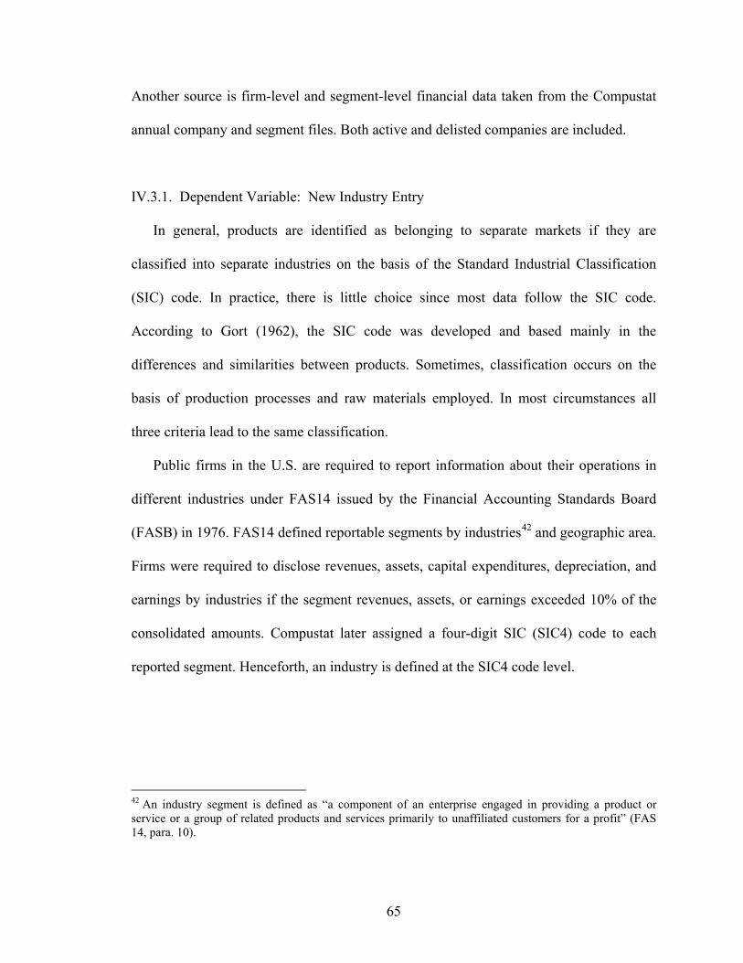
65
Another source is firm-level and segment-level financial data taken from the Compustat
annual company and segment files. Both active and delisted companies are included.
IV.3.1. Dependent Variable: New Industry Entry
In general, products are identified as belonging to separate markets if they are
classified into separate industries on the basis of the Standard Industrial Classification
(SIC) code. In practice, there is little choice since most data follow the SIC code.
According to Gort (1962), the SIC code was developed and based mainly in the
differences and similarities between products. Sometimes, classification occurs on the
basis of production processes and raw materials employed. In most circumstances all
three criteria lead to the same classification.
Public firms in the U.S. are required to report information about their operations in
different industries under FAS14 issued by the Financial Accounting Standards Board
(FASB) in 1976. FAS14 defined reportable segments by industries42 and geographic area.
Firms were required to disclose revenues, assets, capital expenditures, depreciation, and
earnings by industries if the segment revenues, assets, or earnings exceeded 10% of the
consolidated amounts. Compustat later assigned a four-digit SIC (SIC4) code to each
reported segment. Henceforth, an industry is defined at the SIC4 code level.
42 An industry segment is defined as “a component of an enterprise engaged in providing a product or service or a group of related products and services primarily to unaffiliated customers for a profit” (FAS 14, para. 10).
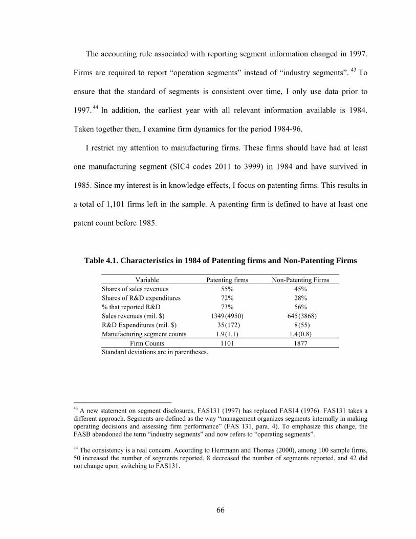
66
The accounting rule associated with reporting segment information changed in 1997.
Firms are required to report “operation segments” instead of “industry segments”. 43 To
ensure that the standard of segments is consistent over time, I only use data prior to
1997. 44 In addition, the earliest year with all relevant information available is 1984.
Taken together then, I examine firm dynamics for the period 1984-96.
I restrict my attention to manufacturing firms. These firms should have had at least
one manufacturing segment (SIC4 codes 2011 to 3999) in 1984 and have survived in
1985. Since my interest is in knowledge effects, I focus on patenting firms. This results in
a total of 1,101 firms left in the sample. A patenting firm is defined to have at least one
patent count before 1985.
Table 4.1. Characteristics in 1984 of Patenting firms and Non-Patenting Firms
Variable Patenting firms Non-Patenting Firms Shares of sales revenues 55% 45% Shares of R&D expenditures 72% 28% % that reported R&D 73% 56% Sales revenues (mil. $) 1349(4950) 645 (3868) R&D Expenditures (mil. $) 35(172) 8 (55) Manufacturing segment counts 1.9(1.1) 1.4 (0.8)
Firm Counts 1101 1877 Standard deviations are in parentheses.
43 A new statement on segment disclosures, FAS131 (1997) has replaced FAS14 (1976). FAS131 takes a different approach. Segments are defined as the way “management organizes segments internally in making operating decisions and assessing firm performance” (FAS 131, para. 4). To emphasize this change, the FASB abandoned the term “industry segments” and now refers to “operating segments”.
44 The consistency is a real concern. According to Herrmann and Thomas (2000), among 100 sample firms, 50 increased the number of segments reported, 8 decreased the number of segments reported, and 42 did not change upon switching to FAS131.
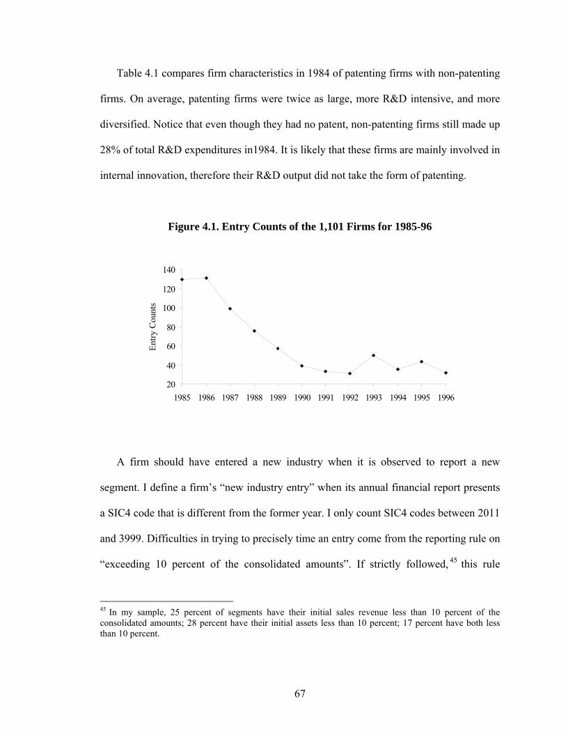
67
Table 4.1 compares firm characteristics in 1984 of patenting firms with non-patenting
firms. On average, patenting firms were twice as large, more R&D intensive, and more
diversified. Notice that even though they had no patent, non-patenting firms still made up
28% of total R&D expenditures in1984. It is likely that these firms are mainly involved in
internal innovation, therefore their R&D output did not take the form of patenting.
Figure 4.1. Entry Counts of the 1,101 Firms for 1985-96
20
40
60
80
100
120
140
1985 1986 1987 1988 1989 1990 1991 1992 1993 1994 1995 1996
Entry
Cou
nts
A firm should have entered a new industry when it is observed to report a new
segment. I define a firm’s “new industry entry” when its annual financial report presents
a SIC4 code that is different from the former year. I only count SIC4 codes between 2011
and 3999. Difficulties in trying to precisely time an entry come from the reporting rule on
“exceeding 10 percent of the consolidated amounts”. If strictly followed, 45 this rule
45 In my sample, 25 percent of segments have their initial sales revenue less than 10 percent of the consolidated amounts; 28 percent have their initial assets less than 10 percent; 17 percent have both less than 10 percent.
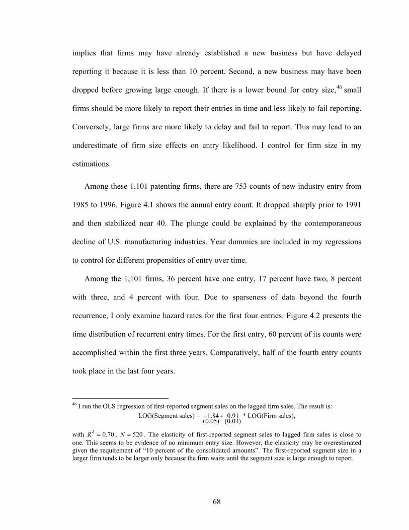
68
implies that firms may have already established a new business but have delayed
reporting it because it is less than 10 percent. Second, a new business may have been
dropped before growing large enough. If there is a lower bound for entry size,46 small
firms should be more likely to report their entries in time and less likely to fail reporting.
Conversely, large firms are more likely to delay and fail to report. This may lead to an
underestimate of firm size effects on entry likelihood. I control for firm size in my
estimations.
Among these 1,101 patenting firms, there are 753 counts of new industry entry from
1985 to 1996. Figure 4.1 shows the annual entry count. It dropped sharply prior to 1991
and then stabilized near 40. The plunge could be explained by the contemporaneous
decline of U.S. manufacturing industries. Year dummies are included in my regressions
to control for different propensities of entry over time.
Among the 1,101 firms, 36 percent have one entry, 17 percent have two, 8 percent
with three, and 4 percent with four. Due to sparseness of data beyond the fourth
recurrence, I only examine hazard rates for the first four entries. Figure 4.2 presents the
time distribution of recurrent entry times. For the first entry, 60 percent of its counts were
accomplished within the first three years. Comparatively, half of the fourth entry counts
took place in the last four years.
46 I run the OLS regression of first-reported segment sales on the lagged firm sales. The result is:
LOG(Segment sales) = 1.84 0.91(0.05) (0.03)− + * LOG(Firm sales),
with 2 0.70R = , 520N = . The elasticity of first-reported segment sales to lagged firm sales is close to one. This seems to be evidence of no minimum entry size. However, the elasticity may be overestimated given the requirement of “10 percent of the consolidated amounts”. The first-reported segment size in a larger firm tends to be larger only because the firm waits until the segment size is large enough to report.
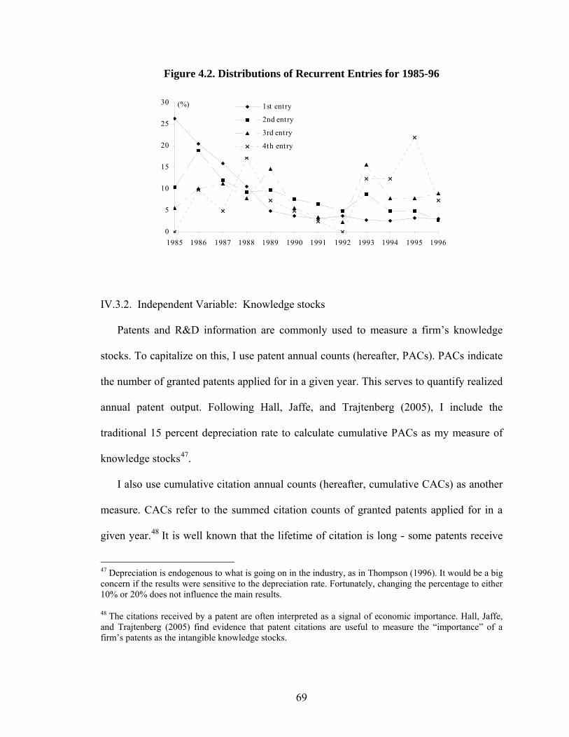
69
Figure 4.2. Distributions of Recurrent Entries for 1985-96
0
5
10
15
20
25
30
1985 1986 1987 1988 1989 1990 1991 1992 1993 1994 1995 1996
(%) 1st entry
2nd entry
3rd entry
4th entry
IV.3.2. Independent Variable: Knowledge stocks
Patents and R&D information are commonly used to measure a firm’s knowledge
stocks. To capitalize on this, I use patent annual counts (hereafter, PACs). PACs indicate
the number of granted patents applied for in a given year. This serves to quantify realized
annual patent output. Following Hall, Jaffe, and Trajtenberg (2005), I include the
traditional 15 percent depreciation rate to calculate cumulative PACs as my measure of
knowledge stocks47.
I also use cumulative citation annual counts (hereafter, cumulative CACs) as another
measure. CACs refer to the summed citation counts of granted patents applied for in a
given year.48 It is well known that the lifetime of citation is long - some patents receive
47 Depreciation is endogenous to what is going on in the industry, as in Thompson (1996). It would be a big concern if the results were sensitive to the depreciation rate. Fortunately, changing the percentage to either 10% or 20% does not influence the main results.
48 The citations received by a patent are often interpreted as a signal of economic importance. Hall, Jaffe, and Trajtenberg (2005) find evidence that patent citations are useful to measure the “importance” of a firm’s patents as the intangible knowledge stocks.
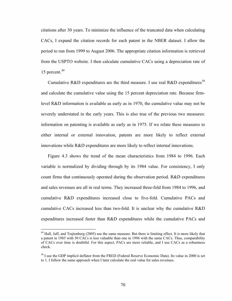
70
citations after 30 years. To minimize the influence of the truncated data when calculating
CACs, I expand the citation records for each patent in the NBER dataset. I allow the
period to run from 1999 to August 2006. The appropriate citation information is retrieved
from the USPTO website. I then calculate cumulative CACs using a depreciation rate of
15 percent.49
Cumulative R&D expenditures are the third measure. I use real R&D expenditures50
and calculate the cumulative value using the 15 percent depreciation rate. Because firm-
level R&D information is available as early as in 1970, the cumulative value may not be
severely understated in the early years. This is also true of the previous two measures:
information on patenting is available as early as in 1975. If we relate these measures to
either internal or external innovation, patents are more likely to reflect external
innovations while R&D expenditures are more likely to reflect internal innovations.
Figure 4.3 shows the trend of the mean characteristics from 1984 to 1996. Each
variable is normalized by dividing through by its 1984 value. For consistency, I only
count firms that continuously operated during the observation period. R&D expenditures
and sales revenues are all in real terms. They increased three-fold from 1984 to 1996, and
cumulative R&D expenditures increased close to five-fold. Cumulative PACs and
cumulative CACs increased less than two-fold. It is unclear why the cumulative R&D
expenditures increased faster than R&D expenditures while the cumulative PACs and
49 Hall, Jaff, and Trajtenberg (2005) use the same measure. But there is limiting effect. It is more likely that a patent in 1985 with 50 CACs is less valuable than one in 1996 with the same CACs. Thus, comparability of CACs over time is doubtful. For this aspect, PACs are more reliable, and I use CACs as a robustness check.
50 I use the GDP implicit deflator from the FRED (Federal Reserve Economic Data). Its value in 2000 is set to 1. I follow the same approach when I later calculate the real value for sales revenues.
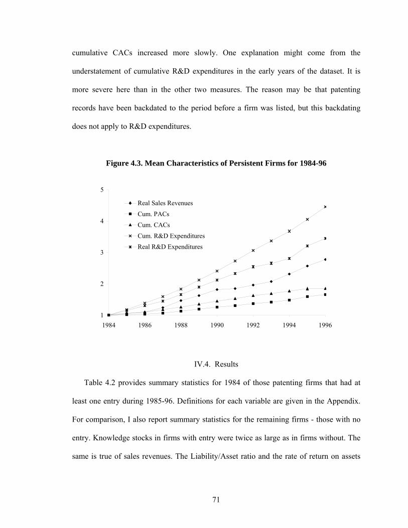
71
cumulative CACs increased more slowly. One explanation might come from the
understatement of cumulative R&D expenditures in the early years of the dataset. It is
more severe here than in the other two measures. The reason may be that patenting
records have been backdated to the period before a firm was listed, but this backdating
does not apply to R&D expenditures.
Figure 4.3. Mean Characteristics of Persistent Firms for 1984-96
1
2
3
4
5
1984 1986 1988 1990 1992 1994 1996
Real Sales Revenues
Cum. PACsCum. CACs
Cum. R&D ExpendituresReal R&D Expenditures
IV.4. Results
Table 4.2 provides summary statistics for 1984 of those patenting firms that had at
least one entry during 1985-96. Definitions for each variable are given in the Appendix.
For comparison, I also report summary statistics for the remaining firms - those with no
entry. Knowledge stocks in firms with entry were twice as large as in firms without. The
same is true of sales revenues. The Liability/Asset ratio and the rate of return on assets
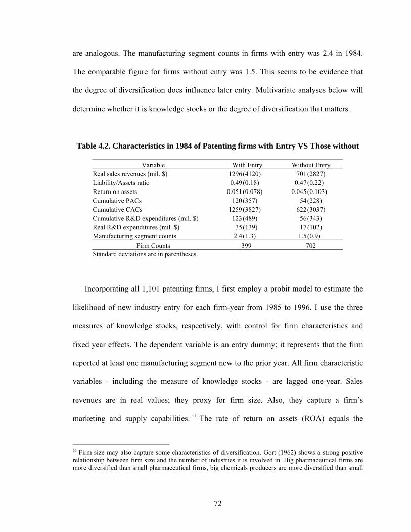
72
are analogous. The manufacturing segment counts in firms with entry was 2.4 in 1984.
The comparable figure for firms without entry was 1.5. This seems to be evidence that
the degree of diversification does influence later entry. Multivariate analyses below will
determine whether it is knowledge stocks or the degree of diversification that matters.
Table 4.2. Characteristics in 1984 of Patenting firms with Entry VS Those without
Variable With Entry Without Entry Real sales revenues (mil. $) 1296(4120) 701 (2827) Liability/Assets ratio 0.49(0.18) 0.47 (0.22) Return on assets 0.051(0.078) 0.045 (0.103) Cumulative PACs 120(357) 54 (228) Cumulative CACs 1259(3827) 622 (3037) Cumulative R&D expenditures (mil. $) 123(489) 56 (343) Real R&D expenditures (mil. $) 35(139) 17 (102) Manufacturing segment counts 2.4(1.3) 1.5 (0.9)
Firm Counts 399 702 Standard deviations are in parentheses.
Incorporating all 1,101 patenting firms, I first employ a probit model to estimate the
likelihood of new industry entry for each firm-year from 1985 to 1996. I use the three
measures of knowledge stocks, respectively, with control for firm characteristics and
fixed year effects. The dependent variable is an entry dummy; it represents that the firm
reported at least one manufacturing segment new to the prior year. All firm characteristic
variables - including the measure of knowledge stocks - are lagged one-year. Sales
revenues are in real values; they proxy for firm size. Also, they capture a firm’s
marketing and supply capabilities. 51 The rate of return on assets (ROA) equals the
51 Firm size may also capture some characteristics of diversification. Gort (1962) shows a strong positive relationship between firm size and the number of industries it is involved in. Big pharmaceutical firms are more diversified than small pharmaceutical firms, big chemicals producers are more diversified than small
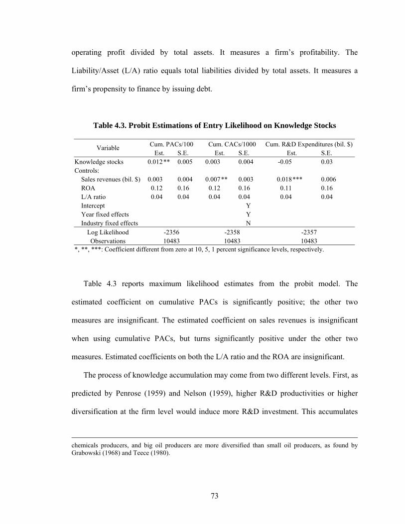
73
operating profit divided by total assets. It measures a firm’s profitability. The
Liability/Asset (L/A) ratio equals total liabilities divided by total assets. It measures a
firm’s propensity to finance by issuing debt.
Table 4.3. Probit Estimations of Entry Likelihood on Knowledge Stocks
Cum. PACs/100 Cum. CACs/1000 Cum. R&D Expenditures (bil. $)Variable Est. S.E. Est. S.E. Est. S.E.
Knowledge stocks 0.012 ** 0.005 0.003 0.004 -0.05 0.03 Controls: Sales revenues (bil. $) 0.003 0.004 0.007** 0.003 0.018 *** 0.006 ROA 0.12 0.16 0.12 0.16 0.11 0.16 L/A ratio 0.04 0.04 0.04 0.04 0.04 0.04 Intercept Y Year fixed effects Y Industry fixed effects N
Log Likelihood -2356 -2358 -2357 Observations 10483 10483 10483
*, **, ***: Coefficient different from zero at 10, 5, 1 percent significance levels, respectively.
Table 4.3 reports maximum likelihood estimates from the probit model. The
estimated coefficient on cumulative PACs is significantly positive; the other two
measures are insignificant. The estimated coefficient on sales revenues is insignificant
when using cumulative PACs, but turns significantly positive under the other two
measures. Estimated coefficients on both the L/A ratio and the ROA are insignificant.
The process of knowledge accumulation may come from two different levels. First, as
predicted by Penrose (1959) and Nelson (1959), higher R&D productivities or higher
diversification at the firm level would induce more R&D investment. This accumulates
chemicals producers, and big oil producers are more diversified than small oil producers, as found by Grabowski (1968) and Teece (1980).
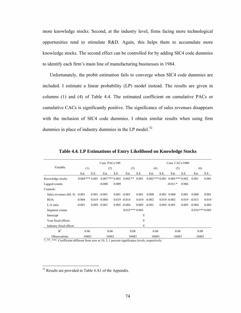
74
more knowledge stocks. Second, at the industry level, firms facing more technological
opportunities tend to stimulate R&D. Again, this helps them to accumulate more
knowledge stocks. The second effect can be controlled for by adding SIC4 code dummies
to identify each firm’s main line of manufacturing businesses in 1984.
Unfortunately, the probit estimation fails to converge when SIC4 code dummies are
included. I estimate a linear probability (LP) model instead. The results are given in
columns (1) and (4) of Table 4.4. The estimated coefficient on cumulative PACs or
cumulative CACs is significantly positive. The significance of sales revenues disappears
with the inclusion of SIC4 code dummies. I obtain similar results when using firm
dummies in place of industry dummies in the LP model.52
Table 4.4. LP Estimations of Entry Likelihood on Knowledge Stocks
Cum. PACs/100 Cum. CACs/1000
(1) (2) (3) (4) (5) (6) Variable
Est. S.E. Est. S.E. Est. S.E. Est. S.E. Est. S.E. Est. S.E.
Knowledge stocks 0.004 *** 0.001 0.007 *** 0.002 0.002** 0.001 0.002 *** 0.001 0.005 *** 0.002 0.001 0.001
Lagged counts -0.008 0.009 -0.011 * 0.006
Controls:
Sales revenues (bil. $) -0.001 0.001 -0.001 0.001 -0.001 0.001 0.000 0.001 0.000 0.001 0.000 0.001
ROA -0.004 0.019 -0.004 0.019 -0.014 0.019 -0.002 0.019 -0.002 0.019 -0.013 0.019
L/A ratio -0.001 0.005 -0.001 0.005 -0.004 0.005 -0.001 0.005 -0.001 0.005 -0.004 0.005
Segment counts 0.033*** 0.003 0.034 *** 0.003
Intercept Y
Year fixed effects Y
Industry fixed effects Y
R2 0.06 0.06 0.08 0.06 0.06 0.08
Observations 10483 10483 10483 10483 10483 10483 *, **, ***: Coefficient different from zero at 10, 5, 1 percent significance levels, respectively.
52 Results are provided in Table 4.A1 of the Appendix.
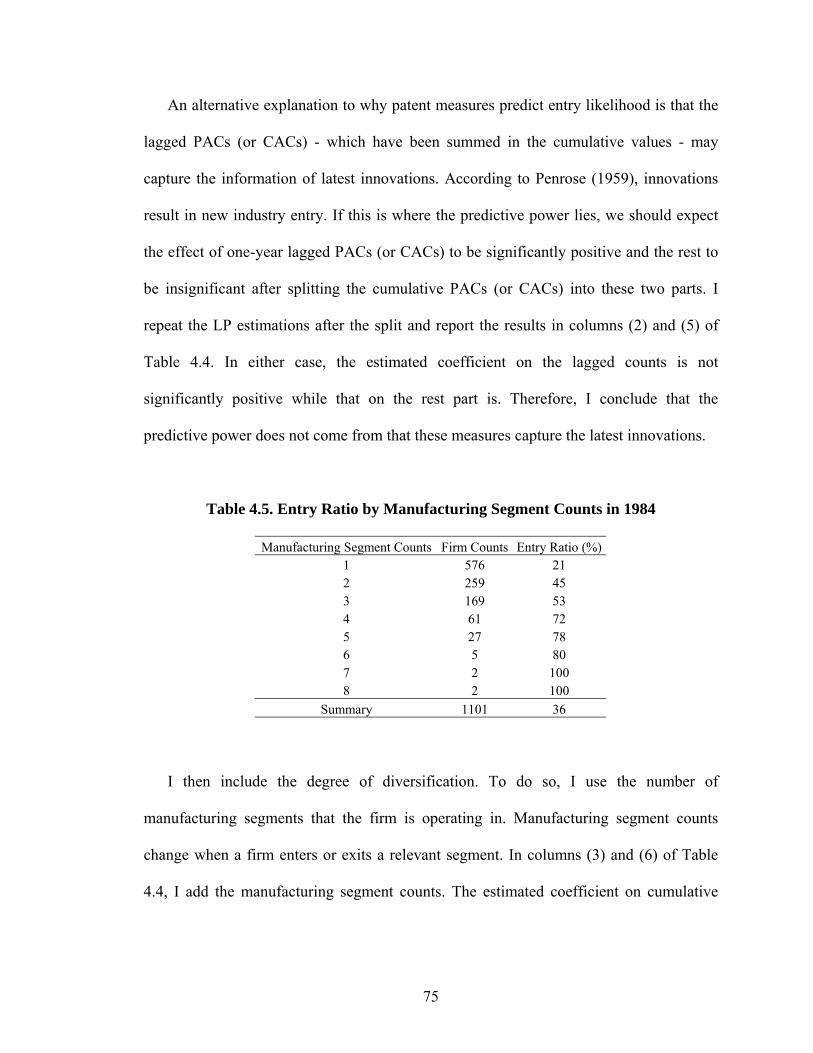
75
An alternative explanation to why patent measures predict entry likelihood is that the
lagged PACs (or CACs) - which have been summed in the cumulative values - may
capture the information of latest innovations. According to Penrose (1959), innovations
result in new industry entry. If this is where the predictive power lies, we should expect
the effect of one-year lagged PACs (or CACs) to be significantly positive and the rest to
be insignificant after splitting the cumulative PACs (or CACs) into these two parts. I
repeat the LP estimations after the split and report the results in columns (2) and (5) of
Table 4.4. In either case, the estimated coefficient on the lagged counts is not
significantly positive while that on the rest part is. Therefore, I conclude that the
predictive power does not come from that these measures capture the latest innovations.
Table 4.5. Entry Ratio by Manufacturing Segment Counts in 1984
Manufacturing Segment Counts Firm Counts Entry Ratio (%) 1 576 21 2 259 45 3 169 53 4 61 72 5 27 78 6 5 80 7 2 100 8 2 100
Summary 1101 36
I then include the degree of diversification. To do so, I use the number of
manufacturing segments that the firm is operating in. Manufacturing segment counts
change when a firm enters or exits a relevant segment. In columns (3) and (6) of Table
4.4, I add the manufacturing segment counts. The estimated coefficient on cumulative
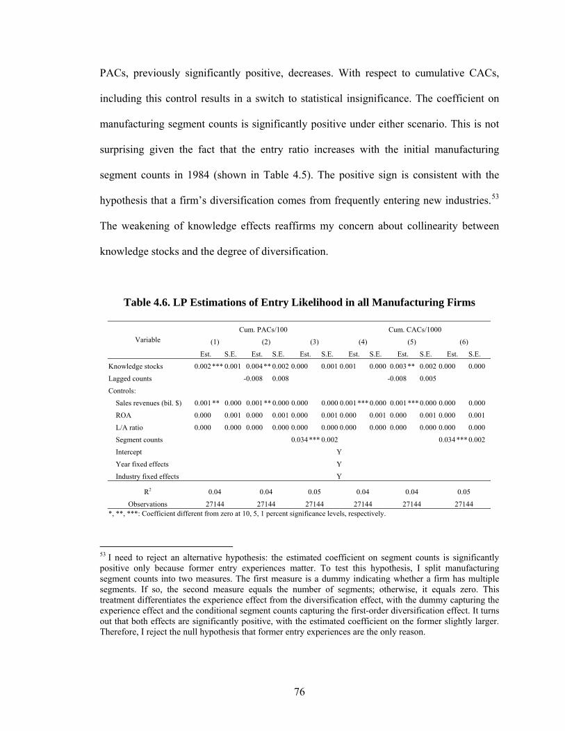
76
PACs, previously significantly positive, decreases. With respect to cumulative CACs,
including this control results in a switch to statistical insignificance. The coefficient on
manufacturing segment counts is significantly positive under either scenario. This is not
surprising given the fact that the entry ratio increases with the initial manufacturing
segment counts in 1984 (shown in Table 4.5). The positive sign is consistent with the
hypothesis that a firm’s diversification comes from frequently entering new industries.53
The weakening of knowledge effects reaffirms my concern about collinearity between
knowledge stocks and the degree of diversification.
Table 4.6. LP Estimations of Entry Likelihood in all Manufacturing Firms
Cum. PACs/100 Cum. CACs/1000
(1) (2) (3) (4) (5) (6) Variable
Est. S.E. Est. S.E. Est. S.E. Est. S.E. Est. S.E. Est. S.E.
Knowledge stocks 0.002 *** 0.001 0.004** 0.002 0.000 0.001 0.001 0.000 0.003 ** 0.002 0.000 0.000
Lagged counts -0.008 0.008 -0.008 0.005
Controls:
Sales revenues (bil. $) 0.001 ** 0.000 0.001** 0.000 0.000 0.000 0.001 *** 0.000 0.001 *** 0.000 0.000 0.000
ROA 0.000 0.001 0.000 0.001 0.000 0.001 0.000 0.001 0.000 0.001 0.000 0.001
L/A ratio 0.000 0.000 0.000 0.000 0.000 0.000 0.000 0.000 0.000 0.000 0.000 0.000
Segment counts 0.034 *** 0.002 0.034*** 0.002
Intercept Y
Year fixed effects Y
Industry fixed effects Y
R2 0.04 0.04 0.05 0.04 0.04 0.05
Observations 27144 27144 27144 27144 27144 27144 *, **, ***: Coefficient different from zero at 10, 5, 1 percent significance levels, respectively.
53 I need to reject an alternative hypothesis: the estimated coefficient on segment counts is significantly positive only because former entry experiences matter. To test this hypothesis, I split manufacturing segment counts into two measures. The first measure is a dummy indicating whether a firm has multiple segments. If so, the second measure equals the number of segments; otherwise, it equals zero. This treatment differentiates the experience effect from the diversification effect, with the dummy capturing the experience effect and the conditional segment counts capturing the first-order diversification effect. It turns out that both effects are significantly positive, with the estimated coefficient on the former slightly larger. Therefore, I reject the null hypothesis that former entry experiences are the only reason.
77
Since those firms with no patent before 1985 shared 28% of the total R&D
expenditures in 1984, I include them in the sample and examine how the results are
influenced. With the inclusion of 1877 non-patenting firms as shown in Table 4.1, I
repeat the LP estimations as in Table 4.4, and report the results in Table 4.6. The
estimated coefficient on sales revenues becomes significantly positive. However, it turns
to be insignificant with the inclusion of Manufacturing segment counts. When using
cumulative PACs as the measure of knowledge stocks, their coefficient is significantly
positive. It also turns to be insignificant with the inclusion of segment counts. When
using cumulative CACs, the coefficient is insignificant except for in column (5) when the
cumulative CACs are splitted into two parts. Diversification effects remain significantly
positive. The weakening of knowledge effects comes from the sample expansion. One
explanation may be that knowledge stocks stimulate innovation productivities only when
the capacity is large enough; thus, including less R&D intensive firms weakens the
average knowledge effects.
Is it possible that the positive relationship between knowledge stocks and entry
likelihood comes from the fact that destination industry R&D attracts diversification, as
asserted by Scherer (1965)? McGowan (1971) provides a reason for this: R&D intensive
industries are often populated by rapidly growing firms. These firms find themselves
short of managerial, financial, and marketing skills. Merging with a diversified firm
remedies this problem. If this is true, the firm in shortage should be the smaller one -
thus, it would be acquired. One likely outcome is that the acquired firm remains listed.
Another outcome could be that it becomes a private sector. In either case, it would not
appear in the data as if the acquired firm had added a new segment. The acquiring firm,

78
however, would have a new entry. However, this hypothesis provides no intuition for its
knowledge characteristics. In conclusion, McGowan’s theory does not explain this
positive relationship.
However, it may be problematic for either the probit or the LP model to assume entry
decisions are made independently across firm-years. In fact, many firms reported more
than one entry during the observation period. Two specific characteristics of these
recurrent entries should be taken into account. First, a firm may already have planned the
second entry before it accomplishes the first one. Second, a firm may enter more than one
industry in a single year.54
Concerned with these characteristics, I adopt the methodology of Wei, Lin, and
Weissfeld (1989) - hereafter referred to as the WLW model. Their treatment of recurrent
failure times imposes no particular structure of dependence between the distinct failure
times of each subject. Each marginal distribution of the failure times takes the form of a
Cox proportional hazards (PH) model. Estimators are asymptotically jointly normal with
a covariance matrix that can be consistently estimated.
Failure time is defined to be an event that adds a new segment. Consider a firm with
no entry in the first year, but two in the second. The event of the second entry is in the
second year, simultaneous to that of the first entry. Firm characteristics, such as real sales
54 Allowing comparison of independent variables over time may lead to underestimation of the positive relationship between knowledge stocks and entry likelihood. For a persistently existing firm, its real sales revenues increase over time, so do knowledge stocks, as shown in Figure 4.3. Meanwhile, most of entries were clustered in the first several years as shown in Figure 4.2.
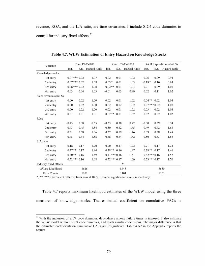
79
revenue, ROA, and the L/A ratio, are time covariates. I include SIC4 code dummies to
control for industry fixed effects.55
Table 4.7. WLW Estimation of Entry Hazard on Knowledge Stocks
Cum. PACs/100 Cum. CACs/1000 R&D Expenditures (bil. $) Variable Est. S.E. Hazard Ratio Est. S.E. Hazard Ratio Est. S.E. Hazard Ratio
Knowledge stocks 1st entry 0.07 *** 0.02 1.07 0.02 0.01 1.02 -0.06 0.09 0.94 2nd entry 0.07 *** 0.02 1.08 0.03 * 0.01 1.03 -0.18 * 0.10 0.84 3rd entry 0.08 *** 0.02 1.08 0.02 ** 0.01 1.03 0.01 0.09 1.01 4th entry 0.03 0.04 1.03 -0.01 0.03 0.99 0.02 0.11 1.02
Sales revenues (bil. $) 1st entry 0.00 0.02 1.00 0.02 0.01 1.02 0.04 ** 0.02 1.04 2nd entry 0.00 0.02 1.00 0.02 0.02 1.02 0.07 *** 0.02 1.07 3rd entry 0.00 0.02 1.00 0.02 0.01 1.02 0.03 * 0.02 1.04 4th entry 0.01 0.01 1.01 0.02 ** 0.01 1.02 0.02 0.02 1.02
ROA 1st entry -0.43 0.38 0.65 -0.33 0.38 0.72 -0.30 0.39 0.74 2nd entry 0.43 0.45 1.54 0.50 0.42 1.65 0.49 0.42 1.63 3rd entry 0.31 0.58 1.36 0.37 0.59 1.46 0.39 0.58 1.48 4th entry 0.45 0.34 1.58 0.48 0.34 1.62 0.50 0.33 1.66
L/A ratio 1st entry 0.18 0.17 1.20 0.20 0.17 1.22 0.21 0.17 1.24 2nd entry 0.37 ** 0.17 1.44 0.38 ** 0.16 1.47 0.38 ** 0.17 1.46 3rd entry 0.40 ** 0.16 1.49 0.41 *** 0.16 1.51 0.42 *** 0.16 1.52 4th entry 0.52 *** 0.16 1.68 0.52 *** 0.17 1.69 0.53 *** 0.17 1.70
Industry fixed effects Y -2*Log Likelihood 8626 8645 8650
Firm Counts 1101 1101 1101 *, **, ***: Coefficient different from zero at 10, 5, 1 percent significance levels, respectively.
Table 4.7 reports maximum likelihood estimates of the WLW model using the three
measures of knowledge stocks. The estimated coefficient on cumulative PACs is
55 With the inclusion of SIC4 code dummies, dependence among failure times is imposed. I also estimate the WLW model without SIC4 code dummies, and reach similar conclusions. The major difference is that the estimated coefficients on cumulative CACs are insignificant. Table 4.A2 in the Appendix reports the results.

80
significant and positive up to the third entry. This indicates that knowledge stocks
contributed to entry likelihood. For the first entry, each addition of 100 cumulative PACs
increased the probability by 7 percent per year. The clustering of the forth entry in the
later years and the sparseness of its counts may be the reason for the insignificance of
cumulative PACs. The coefficient on cumulative CACs is positively significant in the
second and the third entry.
New industry entry may stimulate R&D investment. Thus, any fluctuation in
knowledge stocks may reflect a firm’s early entries. With respect to the hazard of
multiple entries, this would result in an overestimation of knowledge effects. To examine
the seriousness of this endogeneity problem, I run an OLS regression of knowledge
stocks on the current entry dummy with control for fixed year effects and fixed firm
effects. I include firm dummies instead of industry dummies because the focus here is on
the fluctuation of knowledge stocks within a firm. The estimated coefficient on the entry
dummy is insignificant at a significance level of 10 percent. I therefore conclude that
even for multiple entries, overestimation is not a serious problem.
Again I stress that there is no evidence that cumulative R&D expenditures
significantly influence entry likelihood. Based on my model, it indicates that cumulative
R&D expenditures are not a good measure of the knowledge stocks that would favor
external innovations. An explanation is that R&D investment focuses mainly on internal
innovation, and the proportion spent on external innovations is random. This result is also
consistent with my concern that cumulative R&D expenditures may be understated in the
early years. The coefficient on sales revenues achieves significance when using
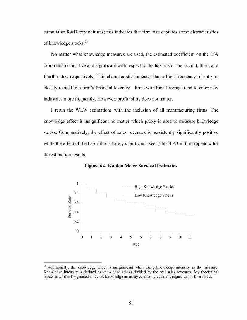
81
cumulative R&D expenditures; this indicates that firm size captures some characteristics
of knowledge stocks.56
No matter what knowledge measures are used, the estimated coefficient on the L/A
ratio remains positive and significant with respect to the hazards of the second, third, and
fourth entry, respectively. This characteristic indicates that a high frequency of entry is
closely related to a firm’s financial leverage: firms with high leverage tend to enter new
industries more frequently. However, profitability does not matter.
I rerun the WLW estimations with the inclusion of all manufacturing firms. The
knowledge effect is insignificant no matter which proxy is used to measure knowledge
stocks. Comparatively, the effect of sales revenues is persistently significantly positive
while the effect of the L/A ratio is barely significant. See Table 4.A3 in the Appendix for
the estimation results.
Figure 4.4. Kaplan Meier Survival Estimates
0
0.2
0.4
0.6
0.8
1
0 1 2 3 4 5 6 7 8 9 10 11
Age
Surv
ival
Rat
e
High Knowledge Stocks
Low Knowledge Stocks
56 Additionally, the knowledge effect is insignificant when using knowledge intensity as the measure. Knowledge intensity is defined as knowledge stocks divided by the real sales revenues. My theoretical model takes this for granted since the knowledge intensity constantly equals 1, regardless of firm size n.

82
I then turn to a survival study of the segments established since 1985. Note that
establishments in 1996 are excluded because there is no information about their survival.
Also excluded are segments with initial assets equal to the contemporary total assets of
their firms.57 This leaves 682 segments distributed in 399 firms; 54 percent have one
entry, 24 percent with two, 13 percent with three, and the others with four and above. I
label a “firm exit” as when an established segment (based on the SIC4 code) is dropped
from the financial report. Under this definition, if a firm terminates its financial report, it
exits all of its business segments. I treat these exits as ordinary.
To proceed, I first separate these 682 segments into two groups, one from high
knowledge firms and the other from low knowledge firms, based on the median
cumulative PACs in 1984. Figure 4.4 shows the estimated segment survival curves of
these two groups. Both survival curves are much flatter than start-up firms. In either
group, half of the segments are still alive when six years old. Segments in high patenting
firms seem to have a survival advantage - albeit quite mild. The following multivariate
analyses determine the importance of knowledge stocks.
MacDonald (1985) and Hall (1988) show that R&D intensive firms are more likely to
enter high R&D industries, which are generally riskier. Even if these firms have some
advantage in survival because of knowledge stocks, this selective entry may offset this. I
therefore include SIC4 code dummies to control for any industry fixed effects that a
segment may be subject to. I also include year dummies to control for the cohort of
establishments. All firm characteristic variables are static and take the value when the
57 I also run the estimations when keeping these segments, and reach similar conclusions.
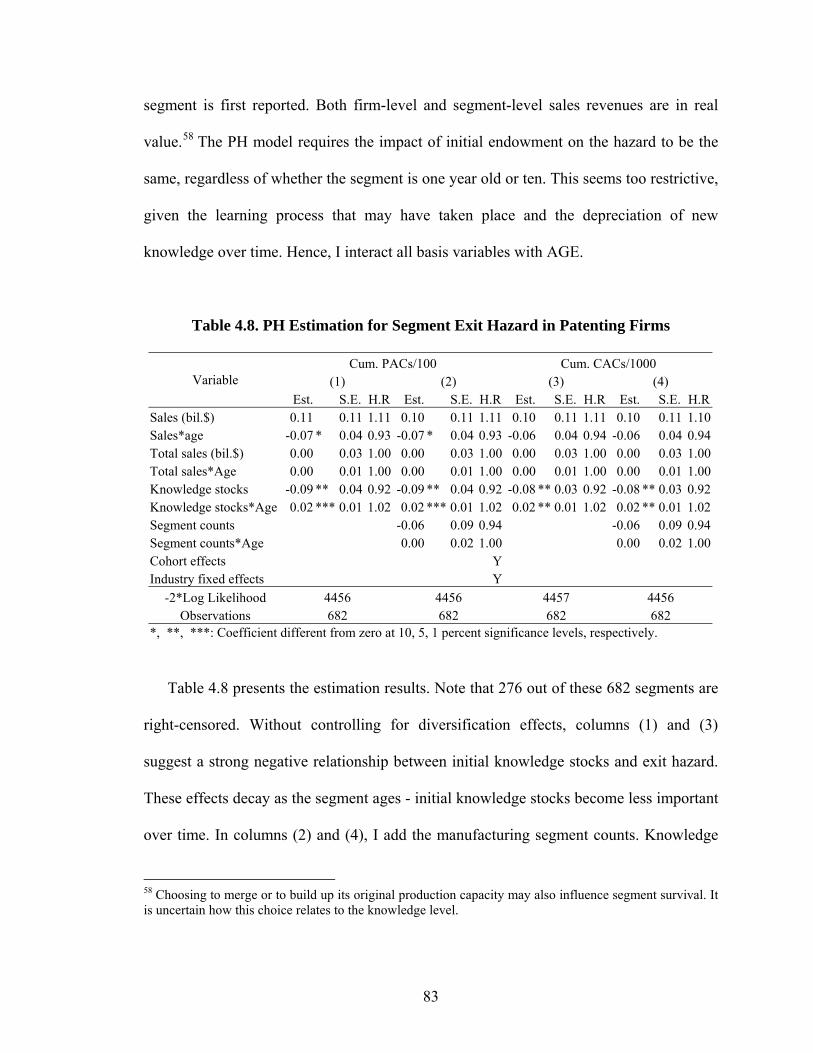
83
segment is first reported. Both firm-level and segment-level sales revenues are in real
value.58 The PH model requires the impact of initial endowment on the hazard to be the
same, regardless of whether the segment is one year old or ten. This seems too restrictive,
given the learning process that may have taken place and the depreciation of new
knowledge over time. Hence, I interact all basis variables with AGE.
Table 4.8. PH Estimation for Segment Exit Hazard in Patenting Firms
Cum. PACs/100 Cum. CACs/1000 (1) (2) (3) (4) Variable
Est. S.E. H.R Est. S.E. H.R Est. S.E. H.R Est. S.E. H.RSales (bil.$) 0.11 0.11 1.11 0.10 0.11 1.11 0.10 0.11 1.11 0.10 0.11 1.10Sales*age -0.07 * 0.04 0.93 -0.07 * 0.04 0.93 -0.06 0.04 0.94 -0.06 0.04 0.94Total sales (bil.$) 0.00 0.03 1.00 0.00 0.03 1.00 0.00 0.03 1.00 0.00 0.03 1.00Total sales*Age 0.00 0.01 1.00 0.00 0.01 1.00 0.00 0.01 1.00 0.00 0.01 1.00Knowledge stocks -0.09 ** 0.04 0.92 -0.09 ** 0.04 0.92 -0.08 ** 0.03 0.92 -0.08 ** 0.03 0.92Knowledge stocks*Age 0.02 *** 0.01 1.02 0.02 *** 0.01 1.02 0.02 ** 0.01 1.02 0.02 ** 0.01 1.02Segment counts -0.06 0.09 0.94 -0.06 0.09 0.94Segment counts*Age 0.00 0.02 1.00 0.00 0.02 1.00Cohort effects Y Industry fixed effects Y
-2*Log Likelihood 4456 4456 4457 4456 Observations 682 682 682 682
*, **, ***: Coefficient different from zero at 10, 5, 1 percent significance levels, respectively.
Table 4.8 presents the estimation results. Note that 276 out of these 682 segments are
right-censored. Without controlling for diversification effects, columns (1) and (3)
suggest a strong negative relationship between initial knowledge stocks and exit hazard.
These effects decay as the segment ages - initial knowledge stocks become less important
over time. In columns (2) and (4), I add the manufacturing segment counts. Knowledge
58 Choosing to merge or to build up its original production capacity may also influence segment survival. It is uncertain how this choice relates to the knowledge level.
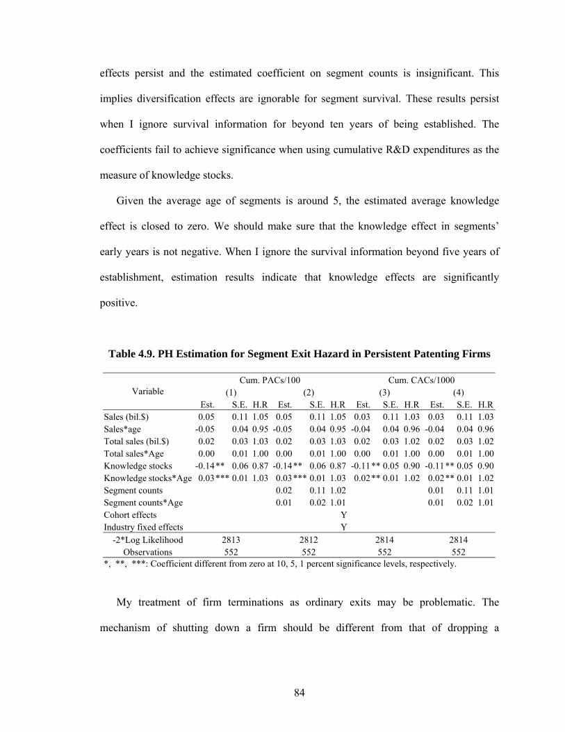
84
effects persist and the estimated coefficient on segment counts is insignificant. This
implies diversification effects are ignorable for segment survival. These results persist
when I ignore survival information for beyond ten years of being established. The
coefficients fail to achieve significance when using cumulative R&D expenditures as the
measure of knowledge stocks.
Given the average age of segments is around 5, the estimated average knowledge
effect is closed to zero. We should make sure that the knowledge effect in segments’
early years is not negative. When I ignore the survival information beyond five years of
establishment, estimation results indicate that knowledge effects are significantly
positive.
Table 4.9. PH Estimation for Segment Exit Hazard in Persistent Patenting Firms
Cum. PACs/100 Cum. CACs/1000 (1) (2) (3) (4) Variable
Est. S.E. H.R Est. S.E. H.R Est. S.E. H.R Est. S.E. H.RSales (bil.$) 0.05 0.11 1.05 0.05 0.11 1.05 0.03 0.11 1.03 0.03 0.11 1.03Sales*age -0.05 0.04 0.95 -0.05 0.04 0.95 -0.04 0.04 0.96 -0.04 0.04 0.96Total sales (bil.$) 0.02 0.03 1.03 0.02 0.03 1.03 0.02 0.03 1.02 0.02 0.03 1.02Total sales*Age 0.00 0.01 1.00 0.00 0.01 1.00 0.00 0.01 1.00 0.00 0.01 1.00Knowledge stocks -0.14 ** 0.06 0.87 -0.14** 0.06 0.87 -0.11** 0.05 0.90 -0.11 ** 0.05 0.90Knowledge stocks*Age 0.03 *** 0.01 1.03 0.03*** 0.01 1.03 0.02** 0.01 1.02 0.02 ** 0.01 1.02Segment counts 0.02 0.11 1.02 0.01 0.11 1.01Segment counts*Age 0.01 0.02 1.01 0.01 0.02 1.01Cohort effects Y Industry fixed effects Y
-2*Log Likelihood 2813 2812 2814 2814 Observations 552 552 552 552
*, **, ***: Coefficient different from zero at 10, 5, 1 percent significance levels, respectively.
My treatment of firm terminations as ordinary exits may be problematic. The
mechanism of shutting down a firm should be different from that of dropping a
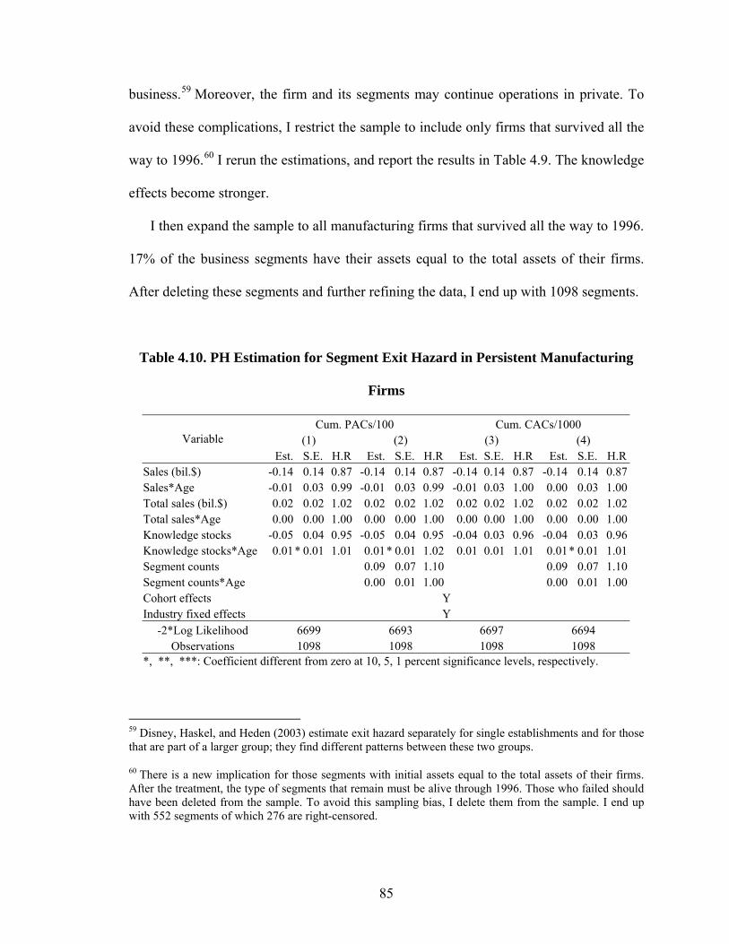
85
business.59 Moreover, the firm and its segments may continue operations in private. To
avoid these complications, I restrict the sample to include only firms that survived all the
way to 1996.60 I rerun the estimations, and report the results in Table 4.9. The knowledge
effects become stronger.
I then expand the sample to all manufacturing firms that survived all the way to 1996.
17% of the business segments have their assets equal to the total assets of their firms.
After deleting these segments and further refining the data, I end up with 1098 segments.
Table 4.10. PH Estimation for Segment Exit Hazard in Persistent Manufacturing
Firms
Cum. PACs/100 Cum. CACs/1000 (1) (2) (3) (4) Variable
Est. S.E. H.R Est. S.E. H.R Est. S.E. H.R Est. S.E. H.RSales (bil.$) -0.14 0.14 0.87 -0.14 0.14 0.87 -0.14 0.14 0.87 -0.14 0.14 0.87Sales*Age -0.01 0.03 0.99 -0.01 0.03 0.99 -0.01 0.03 1.00 0.00 0.03 1.00Total sales (bil.$) 0.02 0.02 1.02 0.02 0.02 1.02 0.02 0.02 1.02 0.02 0.02 1.02Total sales*Age 0.00 0.00 1.00 0.00 0.00 1.00 0.00 0.00 1.00 0.00 0.00 1.00Knowledge stocks -0.05 0.04 0.95 -0.05 0.04 0.95 -0.04 0.03 0.96 -0.04 0.03 0.96Knowledge stocks*Age 0.01* 0.01 1.01 0.01* 0.01 1.02 0.01 0.01 1.01 0.01 * 0.01 1.01Segment counts 0.09 0.07 1.10 0.09 0.07 1.10Segment counts*Age 0.00 0.01 1.00 0.00 0.01 1.00Cohort effects Y Industry fixed effects Y
-2*Log Likelihood 6699 6693 6697 6694 Observations 1098 1098 1098 1098
*, **, ***: Coefficient different from zero at 10, 5, 1 percent significance levels, respectively.
59 Disney, Haskel, and Heden (2003) estimate exit hazard separately for single establishments and for those that are part of a larger group; they find different patterns between these two groups.
60 There is a new implication for those segments with initial assets equal to the total assets of their firms. After the treatment, the type of segments that remain must be alive through 1996. Those who failed should have been deleted from the sample. To avoid this sampling bias, I delete them from the sample. I end up with 552 segments of which 276 are right-censored.
86
I rerun the PH estimations as in Table 4.9, and report the results in Table 4.10.
Among these 1098 segments, 540 are right-censored. The coefficient on initial
knowledge stocks, though keeping a negative sign, shows no statistical significance.
These results persist when I follow the process as in Table 4.8. This difference also
comes from the sample expansion. One explanation may be that new industry entry in
patenting firms follows a mechanism different from that in non-patenting firms: patenting
firms are more likely to enter R&D intensive industries, where knowledge stocks play a
more important role in segment survival.
There is evidence that a firm’s pre-entry background plays an important role in its
survival. According to Klepper and Simons (2000), the surviving firms in the U.S.
television receiver industry were almost exclusively those that had diversified out of
producing radios. Knowledge effects and background effects may be correlated. To
address this background question, I employ a fixed effects estimation procedure.
Unfortunately, the regressions fail to converge when firm dummies are included.
IV.5. Conclusions
By examining U.S. public patenting firms in manufacturing sectors for 1984-96, I
find that knowledge stocks predict the likelihood of a firm’s new market entry. However,
this predictive power is vanished when diversification effects are taken into account. The
diversification effects are significantly positive in predicting entry likelihood. The
knowledge effect is weaker when I include all manufacturing firms in my sample.

87
One shortcoming of my results is that there may involve an endogeneity problem
because of the interactions between knowledge stocks and diversification. The detected
positive significance of knowledge effects may come from the positive correlation of
knowledge stocks and the degree of diversification. Ignoring the endogeneity problem
would lead to overestimation of the coefficient on knowledge stocks.
A survival study of newly established segments in patenting firms shows that initial
knowledge stocks have significantly positive influence on the segments’ later survival.
However, contradictory to traditional findings in plant survival studies, neither initial
segment size, initial firm size, nor degree of diversification shows any significant effect.
When I expand my examination to all manufacturing firms, the hazard estimations of
segment exits show no significant knowledge effects. Meanwhile, diversification effects
are insignificant.
My study provides a preliminary basis for which to select the measure of knowledge
stocks. Patent measures consistently perform better than R&D measures, either in
estimating entry likelihood or in estimating segment exit hazard.
88
References
Audretsch, D., and M. Feldman (1999): “Innovation in Cities: Science-Based Diversity, Specialization and Localized Competition.” European Economic Review 43(2):409-429.
Baldwin, J., and Gu, W. (2005): “The Impact of Trade on Plant Scale, Production-Run Length and Diversification.” Statistics Canada, mimeograph.
Bernard, A. B., and J. B. Jensen. (2007):“ Firm Structure, Multinationals and Manufacturing Plant Deaths.” Review of Economics and Statistics 89(2):193-204.
Disney, R., J. Haskel, and Y. Heden (2003): “Entry, Exit, and Establishment Survival in UK Manufacturing.” Journal of Industrial Economics 51(1):91-112.
Dunne, T., M. J. Roberts, and L. Samuelson (1989a): “The Growth and Failure of U.S. Manufacturing Plants.” Quarterly Journal of Economics 104(4):671-698.
Dunne, T., M. J. Roberts, and L. Samuelson (1989b): “Plant Turnover and Gross Employment Flows in the U.S. Manufacturing Sector.” Journal of Labor Economics 7(1):48-71.
Gollop, F. M., and J. L. Monahan (1991): “A Generalized Index of Diversification: Trends in U.S. Manufacturing.” Review of Economics and Statistics 73(2):318-330.
Gort, M. (1962): Diversification and Integration in American Industry. Princeton: Princeton University Press.
- (1969): “An Economic Disturbance Theory of Mergers.” Quarterly Journal of Economics 83(4):624-642.
Grabowski, H. G. (1968): “The Determinants of Industrial Research and Development: A Study of the Chemical, Drug, and Petroleum Industries.” Journal of Political Economy 76(2):292-306.
Grossman, G. M., and E. Helpman (1991): innovation and Growth in the Global Economy. Cambridge: MIT Press.
Hall, B. (1988): “The Effect of Takeover Activity on Corporate Research and Development.” In Alan Auerbach, ed., Corporate Takeovers: Causes and Consequences. Chicago: University of Chicago Press.
-, A. B. Jaffe, and M. Trajtenberg (2005): “Market Value and Patent Citations.” RAND Journal of Economics 36(1):16-38.

89
Herrmann, D., and W. B. Thomas (2000): “An Analysis of Segment Disclosures under SFAS No. 131 and SFAS No. 14.” Accounting Horizons 14(3):287-302.
Klepper, S., and K. Simons (2000): “Dominance by Birthright: Entry of Prior Radio Producers and Competitive Ramifications in the U.S. Television Receiver Industry.” Strategic Management Journal 21:997-1016.
- and P. Thompson (2006): “Submarkets and the Evolution of market Structure.” RAND Journal of Economics 37(4):862-888.
Klette, T. J., and S. Kortum (2004): “Innovating Firms and Aggregate Innovation.” Journal of Political Economy 112(5):986-1018.
MacDonald, J. M. (1985): “R&D and the Direction of Diversification.” Review of Economics and Statistics 67(4):583-590.
McGowan, J. J. (1971): “International Comparisons of Merger Activity.” Journal of Law and Economics 14(1):233-250.
Montgomery, C. A. (1994): “Corporate Diversification.” Journal of Economic Perspectives 8(3):163-178.
Nelson, R. R. (1959): “The Simple Economics of Basic Scientific Research.” Journal of Political Economy 67(3):297-306.
Penrose, E. (1959): The Growth of the Firm. White Pains, N.Y.: Sharpe.
Scherer, F. M. (1965): “Firm Size, Market Structure, Opportunity, and the Output of Patented Inventions.” American Economic Review 55(5):1097-1125.
- (1983): “The propensity to patent.” International Journal of Industrial Organization 1(1):107-128.
Shaked, A., and Sutton, J. (1990): “Multi-product Firms and Market Structure.” Rand Journal of Economics 21(1):45-62.
Sutton, J. (2005): Competing in Capabilities, Clarendon Lectures. Oxford: Oxford University Press.
Teece, D. (1980): “Economies of Scope and the Scope of the Enterprise.” Journal of Economic Behavior and Organization 1(3):223-247.
Thompson, P. (1996): “Technological Opportunity and the Growth of Knowledge: A Schumpeterian Approach to Measurement.” Journal of Evolutionary Economics 6(1):77-98

90
Wei, L. J., D. Y. Lin, and L. Weissfeld (1989): “Regression Analysis of Multivariate Incomplete Failure Time Data by Modeling Marginal Distributions.” Journal of the American Statistical Association 84(408):1065-1073.
Williamson, O. E. (1979): “Transaction-Cost Economics: The Governance of Contractual Relations.” Journal of Law & Economics 22(2):233-261.

91
Appendix
Variable Description
Specific variables used in the analysis are defined as follows:
. Patent Annual Counts (PACs) is defined as the number of granted patents applied for in a given year.
. Cumulative PACs is the summation of PACs before a given year using a depreciation rate of 15 percent.
. Citation Annual Counts (CACs) is defined as the summed citation counts of granted patents applied for in a given year. Here, citation counts of a patent are the number of citations that the patent received until August 2006.
. Cumulative CACs is the sum of CACs before a given year using 15 percent as the depreciate rate.
. R&D expenditures is R&D expenditures (Compustat item 46) in the fiscal year. In real 2000 values.
. Cumulative R&D expenditures is the sum of real R&D expenditures before a given year using 15 percent as the depreciation rate.
. Sales revenues is sales revenues (Compustat item 12) in the fiscal year. In real 2000 values.
. Ratio of return on assets (ROA) equals operating profit (Compustat item 181) divided by total assets (Compustat item 6).
. Liability/Asset ratio (L/A) equals total liabilities (Compustat item 12) divided by total assets (Compustat item 6).
. Manufacturing segment counts is the number of manufacturing segments (SIC4 codes 2011 to 3999) that the firm is involved in.

92
The Firm’s Innovation Policy
To derive the properties of the innovation policy of a firm with product scope n, I
construct a function
( )
1 1 2 21 2
1 2 1 2
( ) ( )( , ) c x c xf x xr x xπγ γ− −
=− + − +
(4.A1)
The solution (4.6) to the Bellman equation (4.1) implies 1 2( , )f vλ λ = .
I first introduce Lemma 4.1 as follows.
Lemma 4.1: If there is * *1 2( , )x x such that * * * *
1 2 1 1 2 2( , ) '( ) '( )f x x c x c x= = , then * *11 1 2( , ) 0f x x <
and * *22 1 2( , ) 0f x x < .
Proof. The first-order derivatives of 1 2( , )f x x are
( )
1 2 1 11 1 2
1 2 1 2
( , ) '( )( , ) f x x c xf x xr x xγ γ
−=
− + − +, (4.A2)
( )
1 2 2 12 1 2
1 2 1 2
( , ) '( )( , ) f x x c xf x xr x xγ γ
−=
− + − +. (4.A3)
And its second-order derivatives are
[ ] ( ) [ ]
( )1 1 2 1 1 1 2 1 2 1 2 1 1
11 1 2 21 2 1 2
( , ) ''( ) ( , ) '( )( , )
f x x c x r x x f x x c xf x x
r x x
γ γ
γ γ
− − + − + + −⎡ ⎤⎣ ⎦=− + − +⎡ ⎤⎣ ⎦
, (4.A4)
[ ] ( ) [ ]
( )2 1 2 2 2 1 2 1 2 1 2 2 2
22 1 2 21 2 1 2
( , ) ''( ) ( , ) '( )( , )
f x x c x r x x f x x c xf x x
r x x
γ γ
γ γ
− − + − + + −⎡ ⎤⎣ ⎦=− + − +⎡ ⎤⎣ ⎦
. (4.A5)
Given * * * *1 2 1 1 2 2( , ) '( ) '( )f x x c x c x= = , we have * * * *
1 1 2 2 1 2( , ) ( , ) 0f x x f x x= = . Substitute them
into (4.A4) and (4.A5), we have

93
( ) ( )
* * * ** * 1 1 2 1 1 1 1
11 1 2 * * * *1 2 1 2 1 2 1 2
( , ) ''( ) ''( )( , ) 0f x x c x c xf x xr x x r x xγ γ γ γ
− −= = <
− + − + − + − + (4.A4)
( ) ( )
* * * ** * 2 1 2 2 2 2 2
22 1 2 * * * *1 2 1 2 1 2 1 2
( , ) ''( ) ''( )( , ) 0f x x c x c xf x xr x x r x xγ γ γ γ
− −= = <
− + − + − + − + (4.A5)
since ''(.) 0c > .■
I then prove that the optimal innovation policy exists and is unique in Proposition 4.1.
Proposition 4.1: Given that
(1) At the point 02(0, )x such that 0
1 2 2'(0) '( )c c x= with 02 0x ≥ , 0
2 1(0, ) '(0)f x c> and
0 02 2 2(0, ) '( )f x c x> ;61
(2) At the point _ _
1 2( , )x x such that _ _
1 2x x nπ+ = and _ _
1 1 2 2'( ) '( )c x c x= , _ _ _
1 2 1 1( , ) '( )f x x c x< and
_ _ _
1 2 2 2( , ) '( )f x x c x< ;
(3) 1 2 2 2( , ) '( )f x cγ γ< , [ ]1 20,x π γ∀ ∈ − ,
then there exists one and only one solution to (4.6), ( )1 2,λ λ , which is the optimal
innovation policy of the firm.
Proof. First I prove that there exists _ _
0 * *2 1 2 1 2(0, ) ( , ) ( , )x x x x x , such that
* * * *1 2 1 1 2 2( , ) '( ) '( ).f x x c x c x= = Let 1 1 2 1 1( ) ( , ) '( )g x f x x c x= − with 2x satisfying
1 1 2 2'( ) '( )c x c x= . 1( )g x is continuous since each component in it is continuous. With
61 Proposition 4.1 holds when condition (1) changes to: At the point 0
1( ,0)x such that 01 1 2'( ) '(0)c x c= with
01 0x ≥ , 0
1 1( ,0) '(0)f x c> and 01 2( ,0) '(0).f x c>

94
condition (1) and (2), we have (0) 0g > and _
1( ) 0g x < . By the intermediate value
theorem, there exits a point ( )1 2,λ λ with _
1 1(0, )xλ ∈ , such that 1( ) 0g λ = and
1 1 2 2'( ) '( )c cλ λ= .
I then prove the uniqueness of ( )1 2,λ λ . Suppose not, and there is more than one
solution to 1( ) 0g x = . Then the curve 1( )g x should cross the x-axis from negative to
positive at one of the intersections, denoted as 1x∧
. This implies that the first
differentiation 1'( ) 0g x∧
≥ . Therefore, either 11 1 2( , ) 0f x x∧ ∧
≥ or 22 1 2( , ) 0f x x∧ ∧
≥ given
1 1 2 2'( ) '( )c x c x∧ ∧
= . This contradicts Lemma 4.1. Therefore, I prove that the solution to (4.6)
is unique.
It is straightforward that 1 2( , )λ λ is global optimal given its uniqueness. Because
1 1(0, )x λ∀ ∈ , 1( ) 0g x < , thus 1 1 2( , ) 0f x x < and 2 1 2( , ) 0f x x < ; _
1 1 1( , )x xλ∀ ∈ , 1( ) 0g x > , thus
1 1 2( , ) 0f x x > and 2 1 2( , ) 0f x x > . Therefore, 1 2( , )f x x is decreasing when 1x deviates
from 1λ . This ends the proof that 1 2( , )λ λ is global optimal.■
The unique intersection between 1( )g x and the x-axis determines 1λ , and 1( )g x is
downward sloping. An increase of π shifts up 1( )g x , leading to an increasing in 1λ .
Similarly, an increase in r and 1γ , or a decrease in 2γ shifts 1( )g x down, leading to a
decrease in 1λ . A shift up in 1 'c leads to an increase in 1c and an increase in 1 'c . Both
shift down 1( )g x , leading to a decrease in 1λ . Similarly, a shift up in 2 'c leads to a
decrease in 1λ .
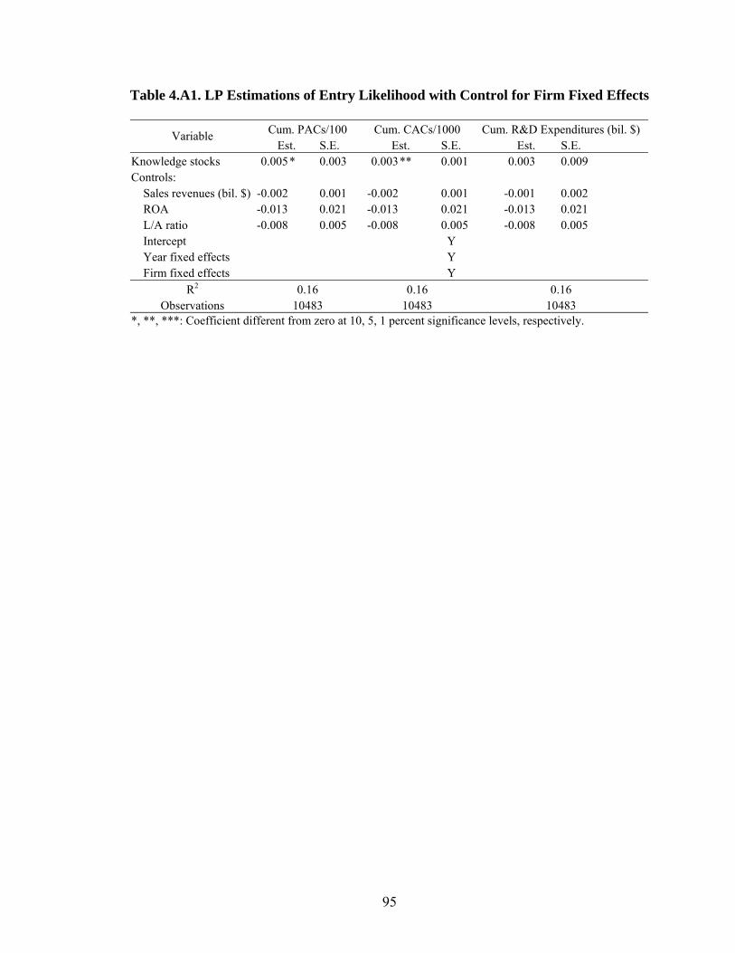
95
Table 4.A1. LP Estimations of Entry Likelihood with Control for Firm Fixed Effects
Cum. PACs/100 Cum. CACs/1000 Cum. R&D Expenditures (bil. $) Variable Est. S.E. Est. S.E. Est. S.E.
Knowledge stocks 0.005 * 0.003 0.003** 0.001 0.003 0.009 Controls: Sales revenues (bil. $) -0.002 0.001 -0.002 0.001 -0.001 0.002 ROA -0.013 0.021 -0.013 0.021 -0.013 0.021 L/A ratio -0.008 0.005 -0.008 0.005 -0.008 0.005 Intercept Y Year fixed effects Y Firm fixed effects Y
R2 0.16 0.16 0.16 Observations 10483 10483 10483
*, **, ***: Coefficient different from zero at 10, 5, 1 percent significance levels, respectively.
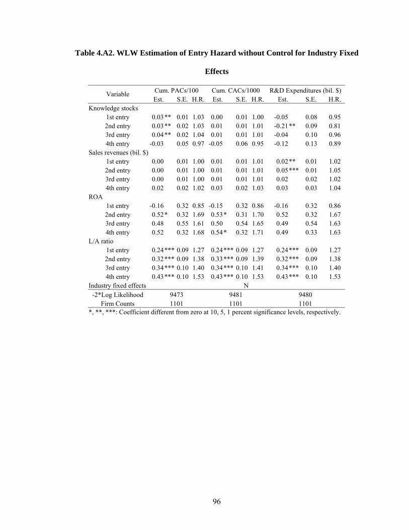
96
Table 4.A2. WLW Estimation of Entry Hazard without Control for Industry Fixed
Effects
Cum. PACs/100 Cum. CACs/1000 R&D Expenditures (bil. $) Variable Est. S.E. H.R. Est. S.E. H.R. Est. S.E. H.R.
Knowledge stocks 1st entry 0.03 ** 0.01 1.03 0.00 0.01 1.00 -0.05 0.08 0.95 2nd entry 0.03 ** 0.02 1.03 0.01 0.01 1.01 -0.21 ** 0.09 0.81 3rd entry 0.04 ** 0.02 1.04 0.01 0.01 1.01 -0.04 0.10 0.96 4th entry -0.03 0.05 0.97 -0.05 0.06 0.95 -0.12 0.13 0.89
Sales revenues (bil. $) 1st entry 0.00 0.01 1.00 0.01 0.01 1.01 0.02 ** 0.01 1.02 2nd entry 0.00 0.01 1.00 0.01 0.01 1.01 0.05 *** 0.01 1.05 3rd entry 0.00 0.01 1.00 0.01 0.01 1.01 0.02 0.02 1.02 4th entry 0.02 0.02 1.02 0.03 0.02 1.03 0.03 0.03 1.04
ROA 1st entry -0.16 0.32 0.85 -0.15 0.32 0.86 -0.16 0.32 0.86 2nd entry 0.52 * 0.32 1.69 0.53* 0.31 1.70 0.52 0.32 1.67 3rd entry 0.48 0.55 1.61 0.50 0.54 1.65 0.49 0.54 1.63 4th entry 0.52 0.32 1.68 0.54* 0.32 1.71 0.49 0.33 1.63
L/A ratio 1st entry 0.24 *** 0.09 1.27 0.24*** 0.09 1.27 0.24 *** 0.09 1.27 2nd entry 0.32 *** 0.09 1.38 0.33*** 0.09 1.39 0.32 *** 0.09 1.38 3rd entry 0.34 *** 0.10 1.40 0.34*** 0.10 1.41 0.34 *** 0.10 1.40 4th entry 0.43 *** 0.10 1.53 0.43*** 0.10 1.53 0.43 *** 0.10 1.53
Industry fixed effects N -2*Log Likelihood 9473 9481 9480
Firm Counts 1101 1101 1101 *, **, ***: Coefficient different from zero at 10, 5, 1 percent significance levels, respectively.
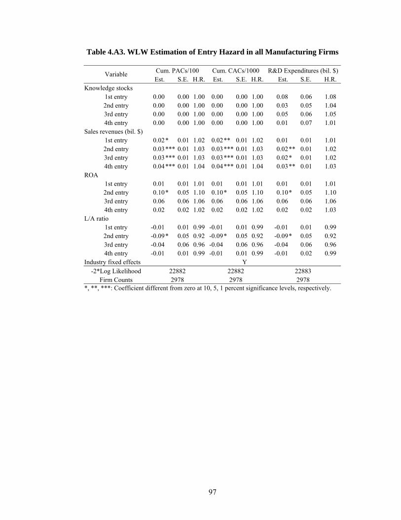
97
Table 4.A3. WLW Estimation of Entry Hazard in all Manufacturing Firms
Cum. PACs/100 Cum. CACs/1000 R&D Expenditures (bil. $)Variable Est. S.E. H.R. Est. S.E. H.R. Est. S.E. H.R.
Knowledge stocks 1st entry 0.00 0.00 1.00 0.00 0.00 1.00 0.08 0.06 1.08 2nd entry 0.00 0.00 1.00 0.00 0.00 1.00 0.03 0.05 1.04 3rd entry 0.00 0.00 1.00 0.00 0.00 1.00 0.05 0.06 1.05 4th entry 0.00 0.00 1.00 0.00 0.00 1.00 0.01 0.07 1.01
Sales revenues (bil. $) 1st entry 0.02* 0.01 1.02 0.02** 0.01 1.02 0.01 0.01 1.01 2nd entry 0.03*** 0.01 1.03 0.03*** 0.01 1.03 0.02 ** 0.01 1.02 3rd entry 0.03*** 0.01 1.03 0.03*** 0.01 1.03 0.02 * 0.01 1.02 4th entry 0.04*** 0.01 1.04 0.04*** 0.01 1.04 0.03 ** 0.01 1.03
ROA 1st entry 0.01 0.01 1.01 0.01 0.01 1.01 0.01 0.01 1.01 2nd entry 0.10* 0.05 1.10 0.10* 0.05 1.10 0.10 * 0.05 1.10 3rd entry 0.06 0.06 1.06 0.06 0.06 1.06 0.06 0.06 1.06 4th entry 0.02 0.02 1.02 0.02 0.02 1.02 0.02 0.02 1.03
L/A ratio 1st entry -0.01 0.01 0.99 -0.01 0.01 0.99 -0.01 0.01 0.99 2nd entry -0.09* 0.05 0.92 -0.09* 0.05 0.92 -0.09 * 0.05 0.92 3rd entry -0.04 0.06 0.96 -0.04 0.06 0.96 -0.04 0.06 0.96 4th entry -0.01 0.01 0.99 -0.01 0.01 0.99 -0.01 0.02 0.99
Industry fixed effects Y -2*Log Likelihood 22882 22882 22883
Firm Counts 2978 2978 2978 *, **, ***: Coefficient different from zero at 10, 5, 1 percent significance levels, respectively.
98
VITA
ZHAO RONG
1993-1997 B.E., Industrial Management Engineering Xi’an Jiaotong University Xi’an, China 1997-2000 M.A., Economics Peking University Beijing, China 2000-2002 Project manager Beijing State-Owned Assets Management Co. Ltd. Beijing, China 2003-2008 Doctoral Candidate in Economics Florida International University Miami, FL, USA PUBLICATION
Rong, Zhao and Yang Yao (2003): “Public Service Provision and the Demand for Electric Appliances in Rural China.” China Economic Review 14(2):131-141.


![Consumption Taxation on Durable Consumer Goods...Consumption Taxation on Durable Consumer Goods 沼田博幸 Hiroyuki NUMA T A [キ}ワード]消費税、付加価値税、耐久消費財、不動産、中古品](https://img.pdfslide.net/doc/110x75/5e7e68e73d2a9a6b3b7c2a80/consumption-taxation-on-durable-consumer-goods-consumption-taxation-on-durable.jpg)