Embed Size (px)
Citation preview

ESSAYS ON INDUSTRIAL ORGANIZATION IN CHINA’S
MANUFACTURING SECTOR
by
Yifan Zhang
B.A., Renmin University of China, 1994
M.A., Renmin University of China, 1997
Submitted to the Graduate Faculty of
Arts and Sciences in partial fulfillment
of the requirements for the degree of
Doctor of Philosophy
University of Pittsburgh
2005

UNIVERSITY OF PITTSBURGH
FACULTY OF ARTS AND SCIENCES
This dissertation was presented
by
Yifan Zhang
It was defended on
August 2, 2005
and approved by
Daniel Berkowitz University of Pittsburgh
Steven Klepper
Carnegie Mellon University
Alexis Leon University of Pittsburgh
Soiliou Namoro
University of Pittsburgh
Thomas Rawski University of Pittsburgh
Dissertation Director
ii

Copyright by Yifan Zhang
2005
iii

ESSYAYS ON INDUSTRIAL ORGANIZATION IN CHINA’S
MANUFACTURING SECTOR
Yifan Zhang, PhD
University of Pittsburgh, 2005
This dissertation consists of three essays that study the industrial organization of China’s
manufacturing sector from an empirical perspective. It focuses on applying industrial
organization theory and econometrics to the analysis of the effects of market forces and
globalization forces on the productivity of China’s manufacturing firms.
Chapter 2 examines theories of vertical specialization dated back to Adam Smith. China’s
economic reform offers an ideal opportunity to test the relationship between the market forces
and vertical specialization of firms. Using a comprehensive firm-level dataset in China’s
manufacturing sector, we find that vertical specialization increases total factor productivity of
firms. Our estimation results support Smith’s extent-of-market theory, Marshall’s input sharing
theory and Coase’s transaction cost theory, but not Stigler’s theory of industry lifecycle. We also
find that transaction cost theory is more powerful than other theories in explaining vertical
specialization of firms. Market reform that facilitates inter-firm transactions is the driving force
behind the vertical specialization process that occurred in China’s manufacturing firms during
the reform period.
Using a panel dataset of China’s manufacturing firms from 2000 to 2003, Chapter 3
examines whether there exist productivity spillovers from foreign direct investment to domestic
firms. In estimating productivity, we control for a possible simultaneity bias by using semi-
parametric estimation techniques. We investigate FDI spillovers through horizontal, backward,
iv

forward and local linkages. Moreover, we allow for different spillover effects depending on the
origin and market orientation of FDI and domestic firms’ absorptive capacity. Our evidence
suggests that FDI in China tends to generate spillovers mainly through backward and local
linkages. We find little evidence of horizontal and forward spillovers.
Chapter 4 analyzes the relationship between firm productivity and export behavior in
China’s manufacturing firms. We find that exporters show superior initial performance relative
to non-exporters, which is consistent with the self-selection hypothesis. Moreover, using
matching and difference-in-difference methods, we find strong evidence supporting the learning-
by-exporting hypothesis. On average, exporting raises the productivity by 13 percent in the first
year.
v

TABLE OF CONTENTS
ACKNOWLEDGEMENTS............................................................................................................ x 1. INTRODUCTION .................................................................................................................. 1
1.1. Background of the Dissertation ...................................................................................... 1 1.2. Vertical Specialization and Firm Performance ............................................................... 2 1.3. FDI and Spillover effects ................................................................................................ 5 1.4. Exporting and Performance ............................................................................................ 7
2. VERTICAL SPECIALIZATION OF FIRMS: EVIDENCE FROM CHINA’S MANUFACTURING SECTOR ................................................................................................... 13
2.1. Conceptual Framework................................................................................................. 13 2.2. Evolution of Vertical Specialization in China’s Industrial Sector................................ 15 2.3. Theories and Hypotheses .............................................................................................. 18
2.3.1. A Theoretical Example ......................................................................................... 18 2.3.2. Developing Hypotheses ........................................................................................ 25
2.4. Measurement and Data ................................................................................................. 31 2.4.1. Measuring Variables ............................................................................................. 31 2.4.2. The Data................................................................................................................ 33
2.5. Empirical Tests ............................................................................................................. 34 2.5.1. Determinants of Vertical Specialization ............................................................... 34 2.5.2. Vertical Specialization and Productivity .............................................................. 38
3. DO DOMESTIC FIRMS BENEFIT FROM FOREIGN DIRECT INVESTMENT? THE CASE OF CHINA......................................................................................................................... 54
3.1. Overview of FDI Spillover Channels ........................................................................... 54 3.1.1. Horizontal Spillovers ............................................................................................ 54 3.1.2. Vertical Spillovers ................................................................................................ 56 3.1.3. Local Spillovers .................................................................................................... 56
3.2. Foreign Direct Investment in China.............................................................................. 57 3.3. Measurement and Data ................................................................................................. 60
3.3.1. Measuring Horizontal Spillovers .......................................................................... 60 3.3.2. Measuring Backward Spillovers ........................................................................... 60 3.3.3. Measuring Forward Spillovers.............................................................................. 61 3.3.4. Measuring Local Spillovers .................................................................................. 61 3.3.5. The Data and Basic Patterns ................................................................................. 61
3.4. Empirical Strategy ........................................................................................................ 63 3.4.1. First Differences Estimation ................................................................................. 64 3.4.2. Semi-Parametric Estimation ................................................................................. 65
3.5. Estimation Results ........................................................................................................ 68 3.5.1. Baseline Specifications ......................................................................................... 68 3.5.2. HMT firms versus OECD firms............................................................................ 69 3.5.3. Technological Gap................................................................................................ 70
vi
3.5.4. Export-Oriented versus Domestic-Market-Oriented FDI ..................................... 71 4. EXPORTING AND PERFORMANCE: FIRM LEVEL EVIDENCE FROM CHINA ....... 85
4.1. Overview of the Literature............................................................................................ 85 4.1.1. Related Theories ................................................................................................... 85 4.1.2. Empirical Studies .................................................................................................. 86
4.2. Growth of China’s Exports ........................................................................................... 87 4.3. The Data and Basic Patterns ......................................................................................... 89 4.4. Testing Self-Selection Hypothesis................................................................................ 90 4.5. Testing Learning-by-Exporting Hypothesis ................................................................. 92
4.5.1. Empirical Strategy ................................................................................................ 92 4.5.2. Estimation Results ................................................................................................ 95
5. CONCLUSIONS................................................................................................................. 104 BIBLIOGRAPHY....................................................................................................................... 107
vii

LIST OF TABLES
Table 2.1 Evolution of Vertical Specialization of China’s Industry (1949-2003)...................... 42 Table 2.2 Evolution of Vertical Specialization by Industry (1980-2000) .................................. 43 Table 2.3 Evolution of Vertical Specialization by Region (1980-2000) .................................... 44 Table 2.4 China’s Ten Youngest and Oldest Industries in 2002 ................................................ 45 Table 2.5 Summary Statistics of the Variables........................................................................... 46 Table 2.6 Determinants of Vertical Specialization ..................................................................... 47 Table 2.7 Determinants of Vertical Specialization: Robustness Checks I.................................. 48 Table 2.8 Determinants of Vertical Specialization: Robustness Checks II ................................ 49 Table 2.9 Determinants of Vertical Specialization: Robustness Checks III ............................... 50 Table 2.10 Determinants of Vertical Specialization ................................................................... 51 Table 2.11 Vertical Specialization and Productivity: OLS Estimation ...................................... 52 Table 2.12 Vertical Specialization and Productivity: IV Estimation.......................................... 53 Table 3.1 Horizontal Spillover Variable by Two-Digit Industry................................................ 73 Table 3.2 Backward Spillover Variable by Two-Digit Industry................................................. 74 Table 3.3 Forward Spillover Variable by Two-Digit Industry ................................................... 75 Table 3.4 Local Spillover Variable by Province......................................................................... 76 Table 3.5 Coverage of the Database ........................................................................................... 77 Table 3.6 Number of Foreign Firms in the Database.................................................................. 77 Table 3.7 Summary Statistics ..................................................................................................... 78 Table 3.8 Additional Summary Statistics of Spillover Variables ............................................... 79 Table 3.9 Firm Differentials of Characteristics between Foreign and Domestic Firms ............. 79 Table 3.10 OLS with Lagged and Contemporaneous Spillover Variables................................. 80 Table 3.11 Regression in First Differences: Baseline Specifications ......................................... 81 Table 3.12 Regression in Second Differences: Baseline Specifications..................................... 82 Table 3.13 Regression in First Differences: Robustness Checks ............................................... 83 Table 3.14 Regression in First Differences: Robustness Checks (Continued) ........................... 84 Table 4.1 The Structure of China’s Exports ............................................................................... 97 Table 4.2 Number of Exporting Firms in the Dataset................................................................. 97 Table 4.3 Export Propensity by Industry (2000-2003) ............................................................... 98 Table 4.4 Firm Differentials of Characteristics between Exporters and Non-Exporters ............ 99 Table 4.5 Determinants of Starting to Export........................................................................... 100 Table 4.6 Matching Estimation of Average Treatment Effect on the Treated (ATT) .............. 101 Table 4.7 Difference-in-Difference Estimation Results (Full Sample) .................................... 101 Table 4.8 Difference-in-Difference Estimation Results (Subsamples)..................................... 102 Table 4.9 Difference-in-Difference Estimation by Selected Industries.................................... 103
viii
LIST OF FIGURES Figure 1.1 Evolution of Vertical Specialization of China’s Industry (1980-2000) .................... 10 Figure 1.2 FDI Inflow into China (1983-2004) .......................................................................... 11 Figure 1.3 China’s Exports (1980-2004) .................................................................................... 12 Figure 2.1 Vertical Specialization Index versus Provincial Marketization Index ....................... 41
ix

ACKNOWLEDGEMENTS
During the course of my Ph.D. study, a long list of mentors, classmates, friends and
family provided many years of support. It is my privilege to express my sincere appreciation to
several people who guided, encouraged, and supported me in the completion of this dissertation.
First in order of gratitude is my dissertation advisor, Professor Thomas Rawski, who
stood solidly behind me during my many years of dissertation work. My understanding of
China’s economy benefited enormously from my work as a research assistant for Prof. Rawski in
the past three years. I also want to thank him for allowing me to use his dataset in the
dissertation.
I would also like to express my sincere gratitude to my dissertation committee. I am
indebted to Prof. Daniel Berkowitz, Prof. Steven Klepper, Prof. Alexis Leon, and Prof. Soiliou
Namoro. I am grateful for their continuous help and guidance in my dissertation research.
The dissertation is dedicated to my family in both China and the U.S., especially to my
wife, Chunmei. Without her support, I could never have reached this point in my life.
x

1. INTRODUCTION
1.1. Background of the Dissertation
In December 1978, the Central Committee of the Communist Party of China held a historic
meeting in Beijing. One of the important decisions made at this meeting was to adopt reform and
open-door policies. The reform policy was aimed at invigorating the economy through market-
oriented reforms. The open-door policy was expected to utilize the opportunities in the
international economy. Since then, China has embarked on a gradual switch from a planned
economy to a market economy and from a closed economy to an open economy. It turned out
that marketization and internationalization became two most fundamental changes in China’s
economy in the past twenty-five years. This dissertation collects three empirical studies aiming at
assessing the impacts of market forces and globalization forces on the China’s manufacturing
firms.
Chapter 2 studies the market forces. It examines the effects of market expansion and
reduction of transaction cost on vertical specialization of firms. We test alternative theories of
vertical specialization dating back to Adam Smith. These widely accepted theories have
surprisingly little empirical support. This chapter attempts to fill the gap in the literature by
exploiting rich variation in regional market development and vertical specialization in China’s
manufacturing sector.
Chapter 3 and Chapter 4 study the globalization forces. We distinguish the impacts of
“passive” internationalization from “active” internationalization. Chapter 3 focuses on “passive”
1

internationalization, looking at the effects of inward foreign direct investment on domestic firms.
Chapter 4 examines “active” internationalization, testing the impacts of active exporting on
firms’ performance.
The rest of Chapter 1 is a brief introduction to the three topics in this dissertation: vertical
specialization, FDI and exporting.
1.2. Vertical Specialization and Firm Performance
When production involves more than one stage, firms must decide whether to vertically
specialize or integrate all stages. The study of vertical specialization goes far back to Adam
Smith’s idea of division of labor. In the very first sentence of Wealth of Nations, Adam Smith
claims that, “the greatest improvement in the productive power of labor, and the greater skill,
dexterity, and judgment with which it is anywhere directed or applied, seem to have been the
effects of the division of labor” (Smith, 1776, Chapter 1). Division of labor allows workers to
exploit their comparative advantage, improve their skills, and increase the efficiency of firms.
Although Adam Smith’s original idea was about specialization within a firm, his insight has been
extended to specialization between firms (Young, 1928; Stigler, 1951).
Adam Smith further claims that division of labor is limited by the extent of market. Based
on this idea, Stigler (1951) discusses the relationship between vertical specialization and industry
lifecycle. He argues that new industries are usually vertically integrated. Then as intermediate-
inputs suppliers enter the market, the degree of vertical specialization rises. In the declining stage
of the lifecycle, the industries become vertically integrated again. Also following the idea of
extent of market, Marshall (1920) explains that industries concentrated in particular regions
2

should be more vertically specialized because input sharing allows the emergence of more
specialized intermediate-inputs suppliers.
Another related theory is the transaction cost literature originated by Coase (1937) and
further developed by Williamson (1975, 1985). Coase argues that a firm will purchase from the
market if the cost of organizing production within the firm is higher than the cost of carrying out
the transaction through the market. Thus, a firm’s vertical specialization decision rests on the
comparison of internal organizational cost and external market transaction cost.
Given the importance of these ideas in economics, one might presume that there is
extensive empirical study on the nature of vertical specialization. Surprisingly, this is not the
case. In particular, at the firm level, there is little systematic evidence quantifying vertical
specialization (Perry, 1989). A rare example of the firm-level empirical evidence on Smith’s idea
that vertical specialization increases productivity appears in Murakami, Liu and Otsuka’s (1996)
study of China’s machine tool industry. There is no firm-level empirical study of Smith’s idea of
extent of market, because existing empirical work focuses either on nation or state level data
(Ades and Glaeser, 1999), or on the division of labor within firms (Ippolito, 1977; Caricano and
Hubbard, 2003). Stigler’s industry lifecycle theory was tested by Tucker and Wilder (1977),
among others, with mixed results. Holmes (1999) finds evidence from U.S. that supports
Marshall’s theory. There are also some studies on agglomeration and input sharing in regional
economics. The transaction cost literature provides relatively abundant firm-level evidence, but
most of it comes from case studies.
There may be two reasons for the lack of empirical study. First, the availability of large
firm-level dataset has always been a major difficulty for researchers (Yang and Ng, 1993, pp.
434-436). Our dataset provides extremely detailed information for all state firms and all non-
3

state firms1 with sales above 5 million Yuan (or about $600,000) in China’s manufacturing
sector in 2002. Total number of firms in our dataset exceeds 160,000. Second, in a mature
market economy like the United States, cross section and time series variations of market
development and vertical specialization are quite small. In the past forty years, the vertical
specialization index of U.S. manufacturing changed by only one percentage point.2 As we see in
Figure 1.1, China’s substantial rise in vertical specialization was accompanied by enormous
growth of market forces during the reform period, which began in the late 1970s. The
development of market system also differed markedly across sectors and regions in China. We
believe that China’s market reform offers a unique opportunity to examine the effects of market
expansion and reduction of transaction cost on vertical specialization of firms.
This dissertation is the first study that examines all the alternative theories simultaneously
and compares their explanatory power. In Chapter 2, using industry size as an instrument for
vertical specialization, we find that an increase in vertical specialization raises total factor
productivity of the firms. Our OLS estimation of the determinants of vertical specialization
supports Smith’s extent-of-market theory, Marshall’s input sharing theory and Coase’s
transaction cost theory. In terms of quantitative significance, our results suggest that transaction
cost may have the largest impact on vertical specialization of firms, which implies that market
reform in China that facilitates inter-firm transactions and reduces transaction cost is the driving
force of the vertical disintegration process after the reform. However, we fail to find strong
evidence in support of Stigler’s industry lifecycle theory.
1 “State firms” include all wholly state-owned firms and state shareholding firms. 2 Vertical specialization index is defined as 1-value added/sales. See discussions in Section 2.1. Vertical specialization index of U.S. manufacturing decreased from 0.54 in 1963 to 0.53 in 2001. Source: Author’s calculation based on Statistical Abstracts of United States (1970) and (2003).
4

1.3. FDI and Spillover effects
One of the primary motivations for governments around the world to attract foreign direct
investment (FDI) is the belief that FDI will generate positive spillovers to domestic firms. World
Bank (1993) writes that “FDI brings with it considerable benefits: technology transfer,
management know-how, and export marketing access. Many developing countries will need to
be more effective in attracting FDI flows if they are to close the technology gap with high-
income countries, upgrade managerial skills, and develop their export markets.” These claims
have encouraged developing countries as well as developed countries to create costly programs,
such as tax breaks, subsidized industrial infrastructure, and duty exemptions, in order to attract
FDI. From 1991 to 2002, developing countries made over 1,500 regulatory changes favorable to
FDI (UNCTAD, 2003, p.21).
Despite its importance to policy choices, recent empirical studies on FDI spillovers find
mixed results. In a summary of the existing evidence, Rodrik (1999, p.37) concludes, “today’s
policy literature is filled with extravagant claims about positive spillovers from FDI, but the hard
evidence is sobering.”
According to the theories, FDI spillovers can work through a number of channels. First,
domestic firms can benefit from the presence of FDI in the same industry, leading to intra-
industry or horizontal spillovers, through labor turnover, demonstration effects, competition
effects, etc. Second, there may be spillovers from foreign firms operating in other industries,3
leading to inter-industry or vertical spillovers. This type of spillover effect is often attributed to
buyer-supplier linkages and therefore may be towards upstream (backward spillovers) or
3 Here “foreign firms” include all firms partly or fully funded by investors from foreign countries as well as Hong Kong, Macao and Taiwan.
5

downstream industries (forward spillovers). Third, domestic firms may also benefit from the FDI
in the same region, leading to local spillovers.
Chapter 3 examines the extent of FDI spillovers using firm-level panel data from China’s
manufacturing sector. China is of particular interest because it is the largest economy among
developing countries, and more importantly the largest recipient of FDI in the world. Guided by
FDI-oriented philosophy, Chinese local governments at all levels compete with each other to
offer tax breaks and other incentives to foreign investors. In the past 25 years, tens of thousands
of global corporations invested in China, bringing with them over 560 billion dollars in FDI.
Figure 1.2 shows the FDI inflow into China between 1980 and 2004.
The general approach in this chapter is to regress firm-level TFP on measures of foreign
presence in the firm’s related industries and region. We use a first differences model to remove
firm-specific unobservable variables. In line with previous studies such as Pavcnik (2002) and
Javorcik (2004), we employ a semi-parametric estimation technique following Levinsohn and
Petrin (2003) to get consistent estimates of total factor productivity (TFP).
We find strong effects of backward and local spillovers. In our study, however, there is
little evidence of horizontal and forward spillovers. We further conduct several robustness
checks. First, we allow the effect of spillovers to differ for overseas Chinese FDI and OECD
FDI. Second, we allow for the heterogeneity of FDI by distinguishing spillovers from primarily
export-oriented and domestic-market-oriented FDI. Third, we allow for different spillover effects
depending on domestic firms’ absorptive capacity. The results of the robustness checks are
consistent with our main findings.
6

1.4. Exporting and Performance
A growing body of empirical literature has documented the superior performance of exporters
relative to non-exporters. The theories suggest at least two mechanisms that can explain a
positive correlation between exporting and productivity. The first is related to self-selection: only
the best firms are able to compete in the international markets. The second explanation is
“learning-by-exporting”: after firms enter the export markets, they gain new knowledge and
expertise that improve their productivity. While the self-selection hypothesis has been confirmed
by various studies, the evidence on the learning hypothesis is mixed. In this dissertation, we
carry out empirical tests for both hypotheses using a large panel dataset from China’s
manufacturing firms.
Learning-by-exporting theory is often cited as an argument for active export promotion
policies such as export subsidies in developing countries. World Bank (1998) writes that,
“improving the policy and business environments to create conditions favorable to trade,
especially exports, is one of the most important ways for countries to obtain knowledge from
abroad.” In particular, the economic success of East Asian economies has been attributed, to a
large extent, to the export-led development strategy. For example, Krueger (1995) argues that the
key distinction between East Asian success and Latin American stagnation is the openness of
international trading regimes in East Asia. Our study sheds some light on these policy issues,
although the hypotheses tested in this chapter are only a subset of the arguments for export
promotion.
There is an ongoing debate on the link between exports and growth. Some economists
believe that exports generate economic growth (e.g., Edwards, 1998) while others argue that the
reality is more complicated and the role of exports overstated (e.g., Rodrik and Rodriguez,
7

2000). Our study contributes to this basically macroeconomic debate by adding microeconomic
evidence.
Being a major exporter in the world, the case of China is of considerable interest in this
context. Since the economic reform started in the late 1970s, China’s government has actively
promoted exports. In 1978, the share of China’s exports in world trade was negligible. After a
quarter century of rapid growth, China surpassed Japan as the world’s third largest trading
economy (behind the United States and Germany) in 2004.4 Figure 1.3 shows the growth of
China exports between 1980 and 2004.
In searching for causal links between exporting and firm productivity, we use propensity
score matching and difference-in-difference techniques developed in microeconometrics (e.g.,
Heckman, Ichimura, and Todd, 1997). Such methods allow us to construct a reasonable
counterfactual and determine the changes in productivity that can be reliably attributed to
exporting.
Our main findings can be summarized as follows. First, we find that Chinese exporters
and non-exporters differ significantly. The exporters tend to have higher TFP but lower labor
productivity. They are larger, less capital intensive and pay higher wages. Second, our estimation
from a probit model shows that more productive firms self-select into export markets. Third, our
difference-in-difference estimates based on matched samples suggest that exporting helps
improve performance. On average, exporting raises the productivity by 13 percentage points in
the first year. The learning effects of exporting last at lest three years. Fourth, we distinguish
foreign invested firms from domestic firms. We find that although multinationals usually have
more international experience and are often closer to the world technology frontier, there are still
4 Source: “China replaced Japan as world’s 3rd largest exporter,” People’s Daily online, April 15, 2005. http://english.people.com.cn/200504/15/eng20050415_181246.html.
8

significant learning effects for foreign invested firms in China. However, compared to domestic
firms, the size of their learning effects is smaller. In summary, our results support both self-
selection and learning-by-exporting theories.
9

Figure 1.1 Evolution of Vertical Specialization of China’s Industry (1980-2000)
0.6260.626
0.643
0.653
0.703
0.691
0.726
0.705
0.727
0.694
0.6
0.65
0.7
0.75
1980 1985 1990 1995 2000
Vert
ical
Spe
cial
izat
ion
Inde
x
Series 1 Series 2
Notes: Vertical specialization index is defined as 1 – Value Added/Gross Output. Series 1 does not control for structural change. Series 2 controls for structural change. In Series 2, 1980 industry output shares are used as weights to calculate weighted average.
Sources: 1980 and 1985 Author’s calculation based on Industry Volume, The Data of Industrial Census of People’s Republic of China in 1985.
1990 Author’s calculation based on China Statistical Yearbook (1991). 1995 Author’s calculation based on Industry Volume, The Data of Third National Industrial Census of
People’s Republic of China in 1995. 2000 Author’s calculation based on China Statistical Yearbook (2001).
10

Figure 1.2 FDI Inflow into China (1983-2004)
Unit: Billion US Dollars
0
10
20
30
40
50
60
70
1983 1984 1985 1986 1987 1988 1989 1990 1991 1992 1993 1994 1995 1996 1997 1998 1999 2000 2001 2002 2003 2004
Sources: 1983-2003: China Statistical Yearbook, 1988, 1995, 2004;
2004: Statistical Communiqué National Economic and Social
of the People’s Republic of China on the 2004
Development, www.stats.gov.cn/english/newrelease/statisticalreports/t20050228_402231957.htm.
11

Figure 1.3 China’s Exports (1980-2004) Unit: Billion US Dollars
0
100
200
300
400
500
600
700
1980 1981 1982 1983 1984 1985 1986 1987 1988 1989 1990 1991 1992 1993 1994 1995 1996 1997 1998 1999 2000 2001 2002 2003 2004
Sources: 1980-2003: China Statistical Yearbook, 1991, 2004;
2004: Statistical Communiqué of the People’s Republic of China on the 2004 National Economic and Social
Development, www.stats.gov.cn/english/newrelease/statisticalreports/t20050228_402231957.htm.
12

2. VERTICAL SPECIALIZATION OF FIRMS: EVIDENCE FROM CHINA’S
MANUFACTURING SECTOR
2.1. Conceptual Framework
two or more sequential stages; (2)
two or
the same
city, ve
I),
defined as the ratio of intermediate inp of intermediate
inputs and value added, VSI is also equal to one minus the ratio of value added to sales. Thus,
Vertical specialization occurs when: (1) a good is produced in
more firms provide value added during its production. “Vertical disintegration” and
“outsourcing” are common synonyms conveying similar idea.5
Technology is probably the most important determinant of vertical specialization. Some
industries are less decomposable than others. A typical example is the energy saving from not
having to reheat steel in the production of steel sheet. Technology explains why even in
rtical specialization of firms varies widely by industry. In the regression, we will include
two-digit industry dummies to control for the industry-specific technology differences.
Our measure of vertical specialization of firms is the vertical specialization index (VS
uts to sales. Since total sales are the sum
5 There is a closely related but different concept of vertical specialization in international trade literature. Rather than produce final products, countries increasingly specialize in particular stages of production (Yi, 2003). This leads to discussions of vertical specialization spanning regions or countries. It differs from our concept which focuses on specialization among firms. To illustrate the difference, suppose a multinational firm operates several subsidiaries in different countries. Vertical specialization of countries occurs if these subsidiaries constitute a global vertical production chain. According to our definition, however, vertical specialization is zero because this activity is confined within a single firm.
13

,1Y
VAYMVSI −== (2.1)
where M is intermediate inputs, VA is value added, and Y is sales. If a firm were entirely
vertically integrated,
have lower VSI than a firm in later stages of production. This limitation complicates cross-
ining
and utilities and focus only on manufacturing sector. In addition, our two-digit industry dummies
no change in vertical specialization. This is particularly relevant in China. Before reform, the
liberalized price system, the relative prices of raw materials rose rapidly. Since an increase in the
evolution of VSI in China’s industrial sector, we include the mining and utilities industries and
The use of VSI was pioneered by Adeleman (1955). Despite these shortcomings, it is
re (see, for example, Tucker and Wilder, 1977; Levy,
1984; Holmes, 1999).
VSI would be zero. Over time, an increase (decrease) in VSI suggests that a
firm has become more vertically specialized (integrated).
However, VSI is not a perfect measure of vertical specialization. First, given the same
amount of value adding activity, a firm that specializes in the earlier stages of production will
sectional comparison of industries or firms. In the regression analysis, we will exclude m
in the regression should control for the positions of industries in the production chain.
Second, a change in relative prices of final products will change VSI even when there is
prices of raw materials such as coal were artificially depressed by the government. When reform
relative prices of raw materials tends to raise VSI in the downstream sectors, time-series
comparison of VSI requires caution. To deal with this problem, in Section 2.2, when we study the
control for structural change by using 1980 fixed industry weights.
widely accepted and used in the literatu
14

2.2. Evolution of Vertical Specialization in China’s Industrial Sector
After the People’s Republic of China was founded in 1949, Chinese economic system was
modeled on the Soviet planned economy. Vertical integration of firms was a hallmark of China’s
industrial structure under planning system.6 As shown by Table 2.1, VSI defined by net value
decreased from 0.68 in 1949 to 0.62 in 1970 and remained below 0.65 in the 1970s.7 Vertically
integrated firms were often referred to as “big and complete” or “small and complete.” In 1976,
for example, 80 percent of over 6,100 firms under the supervision of the First Machinery
Ministry were “full-function” firms (Ji and Rong, 1980). Because Chinese firms relied heavily
on self-supply, most of the large and medium firms even built their own schools and hospitals. It
is widely acknowledged by Chinese economists that such production structure of firms fails to
reach the optimal scale and scope (Sheng, 1994, pp. 1-5). Chinese government began to address
this problem as early as the 1950s. However, little progress had been made until the reform
began in the late 1970s (Rawski, 1980).
Why do firms in planned economies tend to be more vertically integrated than their
market economy counterparts? Coase’s idea of transaction cost can be applied to socialist firms
with slight modification. Although there is no formal market transaction in a planned economy,
other types of external transaction costs do exist and can be very high. According to Kornai
(1980), Soviet-type firms face chronic vertical shortage as well as horizontal shortage (pp. 200-
201). In the presence of vertical shortage, firms’ requests for resources are frequently turned
down by administrative authority because the sum of claims often exceeds the quantity available
6 The lack of vertical specialization is a universal problem of all socialist economies. See, for example, Berliner (1957) and Granick (1960) for the Soviet Union, and Rawski (1980) and Sheng (1994) for China. 7 China’s statistical system did not report value added until 1992. Net value = value added -- depreciation (National Statistical Bureau, 1992).
15

to the authority. Even if the administrative authority meets the requests, firms still face horizontal
shortage. In the relationship of seller and buyer, refused orders, long waiting time and forced
substitution are not unusual. In order to get full supply on time, firms must bargain with
administrative authority and suppliers. When such costs exceed in-house organizational cost, it is
optimal for the firms to produce intermediate inputs internally. Coase’s original idea is to
compare the costs associated with hierarchy and market. In a planned economy, firm’s decision
is actually based on comparing internal hierarchy cost with external hierarchy cost. Our
explanation here is consistent with the behavior of Chinese firms. Rawski (1980) finds that
before reform, Chinese managers often preferred to make rather than buy inputs because they
wanted to reduce the dependence on potentially unreliable suppliers (p. 128).
China’s tax system borrowed from the Soviet Union was based on sales taxes (Wong and
Bird, 2004). By taxing the portion of sales, the product taxes or industrial-commercial taxes
encouraged vertical integration within firms. In 1994, Chinese government replaced the old tax
system with value added taxes and eliminated such distortionary effect.
When reform began in the late 1970s, markets emerged and developed quickly. As a
result, state firms purchased more and more intermediate inputs through markets. In the
machinery industry, for example, thousands of parts production units within those “full-function”
firms were spun off during the “sixth five-year plan” period between 1981 and 1985 (He, 1990,
p. 92). The government also merged different firms’ production units with similar products into
“specialized firms” (He, 1990, pp. 94-96). In addition, new foreign firms, private firms and
township and village enterprises entered the markets of intermediate inputs, supplying
specialized products to state firms.
16

Murakami, Liu and Otsuka (1996) study a survey of 44 firms in China’s machine tool
industry. They find a positive relationship between production efficiency and purchased parts
ratio in 1991 but not in 1980. Their results suggest that at the beginning of the reform, vertical
integration production structure still had an advantage over vertical specialization. The
comparative advantage of vertical integration declined gradually and almost disappeared in the
1980s.
Figure 1.1 illustrates the evolution of VSI in China’s industrial sector after reform. The
VSI continued to rise between 1980 and 1995 and declined slightly after 1995. There are two
possible reasons why the trend was reversed after 1995. First, China National Statistical Bureau
(NBS) changed the definition and coverage of gross industrial output in 1995 (for details, see
NBS, 1997, pp. 89-106). The new definition reduced the level of 1995 gross industrial output by
about 10 percent (Third National Industrial Census Office, 1997, p. 46). Second, in 1998, NBS
revised its statistical system to limit the coverage to state firms and those non-state firms
reporting more than 5 million Yuan in annual sales. To the extent that smaller firms are more
vertically specialized, excluding small non-state firms may lower VSI.
Since the change in industry structure and relative price may affect VSI, we control for
the structural change by calculating industry weighted average of VSI with weights being 1980
industry output shares. As shown in Series 2 of Figure 1.1, controlling for structural change does
not make much difference.
The evolution of vertical specialization of two-digit industries is reported in Table 2.2.
Between 1980 and 2000, the largest increase in VSI occurred in petroleum processing, coking
products and gas production. During the twenty-year period, 27 out of 31 two-digit industries
became more vertically specialized.
17

Table 2.3 documents the regional evolution of VSI between 1980 and 2000. Zhejiang was
the most vertically specialized province in 2000, followed by Tianjin, Jiangsu, Shanghai, and
Guangdong, all located in the most developed coastal region. The five least vertically specialized
regions in 2000 were Tibet, Yunnan, Heilongjiang, Xinjiang and Inner Mongolia, all located in
interior regions that form part of China’s land borders. The last two rows of Table 2.3 compare
coastal regions with non-coastal regions. In 1980, the coastal regions were not very different
from non-coastal regions in terms of vertical specialization. After twenty years of reform, the
average VSI of coastal regions was 8.1 percentage points above that of non-coastal regions in
2000. Actually, the average VSI of non-coastal regions even decreased between 1980 and 2000.
2.3. Theories and Hypotheses
Theories of vertical specialization address two questions. First, what determines the degree of
vertical specialization across firms? Second, does vertical specialization improve firms’
productivity? In this section, we first introduce a simple model of vertical specialization that
attempts to answer both questions. Then on the basis of existing theories and the model, we
develop testable hypotheses.
2.3.1. A Theoretical Example
In a very influential paper, Dixit and Stiglitz (1977) construct a theoretical model of competition
under increasing returns. In the Dixit-Stiglitz framework, Holmes (1999) develops a model that
shows the relationship between geographic concentration and vertical specialization. Here we
incorporate the transaction cost and labor productivity into the model and use it to derive
predictions that are consistent with major theories of vertical specialization.
18

Assume there is only one industry in the economy, which is populated by L individuals.
Each individual is endowed with one unit of labor. Only one firm produces final good but there
are many intermediate good producers. There is a continuum of intermediate goods that are
differentiated and indexed by . Each intermediate good producer specializes in the
production of one good. We further assume that in the equilibrium there is only one producer of
each intermediate good. The final-good producer uses labor and intermediate goods to produce
final good that will be consumed by all L individuals. In this context, the final-good producer can
be a car assembly firm, purchasing various auto parts manufactured by specialized firms.
]1,0[∈x
The production function of the final good is specified as follows:
( ) ,)()(, 1 ρα⎟⎟
⎠⎜⎜
⎝= ∫− dxxmlxmlf
where l is the labor directly used in final good production and )(xm denotes the quantity of
1α
0
ρ⎞⎛ (2.2)
intermediate good x. The production function has a Cobb-Douglas form
where M can be treated as a composite intermediate good
: ( ) ααMlMlf −= 1, ,
and its production function is given by
,)( ρ⎟⎟
⎜⎜= ∫ dxxmM (2.3)
11
0
ρ
⎠
⎞
⎝
⎛
The CES-type functional form of M has important properties of constant returns to scale
and constant elasticity of substitution.
The technology allows firms to produce one unit of intermediate good with one unit of
labor. The final-good firm can produce intermediate goods by itself. Alternatively, it can
purchase intermediate goods from the specialized firms.
19

If intermediate goods are manufactured within the final-good firm, there is an extra cost
of γ units of labor that is proportional to the quantity produced. This additional cost is needed to
coordinate the production of different goods. Thus, in-house production of units of
intermediate good x costs the final-good firm
)(xm
)()1( xmγ+ units of labor. We assume
that 1)1( >>+ρ
γ . Basically this assumption states that the coordination cost should be high
enough to guarantee the existence of the equilibrium. Specialized intermediate-good firms do not
have coordination cost because they produce only one good. However, a fixed set-up cost of
1
θ
units of labor occurs when the firm is establi . In addition, there is a transaction cost ofshed δ
units of labor that is devoted to contract negotiation or contract enforcement. Assume δ is fixed
and independent of quantity produced. For simplicity, we further assume that specialized firms
bear all the transaction cost. Therefore, the labor cost of units of interm x
equal to
)(xm ediate good is
( )δθ ++)(xm if the good is produced in a specialized firm. It can be easily seen that the
The final good is taken as the numeraire (price set to unity). Let w denote the price of
labor in ter
marginal cost of specialized firms is lower, while the disadvantages of specialized firms are the
fixed set-up cost and transaction cost.
ms of final good. Without loss of generality, assume all the intermediate goods
produced by
intermediate good x. The remaining intermediate goods indexed s to 1 are produced by the final-
good firm.
The final-good firm maximizes its profit by choosing labor l and a vector of intermediate
goods:
specialized firms are indexed between 0 and s. Let )(xp be the price of specialized
20

.)()1()()()(max0
11
0
⎫
⎪⎨
⎧
−−⎟⎠
⎜⎝
∫ ∫∫s
dxxmxpdxxml1
⎪⎭
⎪⎬
⎩
⎪−+⎟
⎞⎜⎛
−s
wldxxwmγρα
ρα (2.4)
The first term is the value of total output. The second term is final-good firm’s total
expenditure on specialized intermediate goods. The third term is total labor cost associated with
producing intermediate goods within the firm. It is equal to the sum of quantity of labor used in
internal production and coordination, )()1( xmγ+ , multiplied by labor price, w. The last term is
total cost of labor directly applied in final-good production.
Given the symmetry of the intermediate goods, let and be the equilibrium output
price of a representative specialized intermediate good and represent the equilibrium
output of a typical internally produced interm
and yields the following first order conditions
Sm Sp
and Im
ediate good. Taking derivatives with respect to Sm
Im
,)( 11
0⎟⎠
⎜⎝
and
1SS pmdxxml =⎟
⎞⎜⎛
−
−
− ∫ ρρρα
ραα (2.5)
.)1()( 11
1 ρρρα
ρα ⎟⎞
⎜⎛
−
−
−
0
wmdxxml I γα +=⎟⎠
⎜⎝∫ (2.6)
Equations (2.5) and (2.6) imply that
.)1(1
SS
I wm γρ
+=⎟⎟
⎞⎜⎜⎛
−
(2.7) pm ⎠⎝
With constant elasticity, Dixit and Stiglitz (1977) give the standard result to pin down
: profit maximization of specialized firms implies that price is a constant markup over Sp
21

marginal cost, or ρwp = . AssumiS ng free entry, we can derive the zero profit condition for
specialized firms
).( δθρ S
wm
e left-hand side is sales revenue and the right-hand side is total cost. Solving (2.8)
for equilibrium output
++=S mw (2.8)
Here th
of the specialized intermediate good gives
.)(1 ρ
δθρ−+
=Sm (2.9)
Plugging ρ
pS = into (2.7) yields w
[ ] .)1( 11
SI mm −+= ρργ (2.10)
Since our final-good production function is Cobb-Dougla
show that the equilibrium quantity of labor directly applied to final good production
equals
s form in nature, it is easy to
*l
L)1( α− . The rest of labor in the economy is allocated to the production of intermediate
goods. Thus we have
.)1)(1()( Lmsms IS αγδθ =+−+++ (2.11)
Recall that s is the measure of the set of differentiated intermediate goods that are
produced by specialized firms. Plugging (2.9) and (2.10) into (2.11) and solving for s give
[ ]
[ ].
1
)1()1()(
1
1−++−+
)1( 1−
=ρργγ
δθρ
)1()1( 1−++− ρργγρ
ραL
s (2.12)
22

Given the assumption that 11)1( >>+ γ , it is straightforward to show ρ
[ ] 0)1()1(11 >++− −ρργγ
ρ and therefore
10>
∂∂Ls . Our result is consistent with Adam Smith’s
extent-of-market theory: when the industry size (em loyment in the model) increases, more
intermediate goods will be produced by specialized firms.
p
L. s will be zero if Since ]1,0[∈s , we have two critical values for
[ ] .)1()1()( 1
1
L 1 ραργδθρ ρ
−++
=≤ −L (2.13)
And 1=s when
.)1(2 ρα
δθ−+
=≥ LL (2.14)
To summarize, when the industry size is small, all intermediate goods will be produced
internally by the final-good producer. After industry size exceeds , the range of intermediate
goods produced by final-good firm decreases and specialized firms begin to produce some
intermediate goods. If the industry size is larger than , all intermediate goods will be produced
by specialized firms. The following prediction summarizes the discussion.
Prediction 1: When
1L
2L
,21 LLL ≥≥ 0>∂∂Ls .
o theory. From (2.12), it is straightforward to
show th
The m del also supports transaction cost
e following prediction.
Prediction 2: Under the assumptions in the model, 0<∂∂δ
.
This prediction implies that the final-good producer will spin off
s
more intermediate
goods production to specialized firms when transaction cost is lower.
23

Now let us examine the relationship between productivity and vertical specialization. In
equilibrium, total income equals total output of final good. So we have the following equation
[ ] [ ] .)1()1()1( 11 ρ
αρ
ρρ
ρα ργ⎭⎬⎫⎧ +− −
−Sms (2.15)
Solving (2.11) for L and plugging it into (2.15) lead to an expression for w
α⎩⎨ +−= SsmLwL
[ ] .)1()1()1(
)1(
11 ρ
ρα
ρρ
ααα ργραα
−
−−−
⎭⎩
Since
⎬⎫
⎨⎧ +−+−= ssw (2.16)
11)1( >>+ γ , we have the following prediction. ρ
Prediction 3: Under the assumptions in the model, 0>∂∂
sw .
B d as wage rate or labor productivity, the model predicts that a ecause w can be interprete
higher degree of vertical specialization raises living standard or productivity.
Our measure of vertical specialization equals intermediate inputs/sales. In the model, we
have
./wL
After rearrangement, (2.17) implies that
pwsmVSI S= (2.17)
[ ] [ ].
)1()1(1 11 −− ++⎭⎬
⎩⎨ +−
=ρρ
ρρ
ργργ ⎫⎧α
ns
sVSI (2.18)
It is easy to verify that VSI is strictly increasing in s. However, the nonlinear relationship
between VSI and s illustrates the complications of VSI in measuring vertical specialization of
firms.
24

2.3.2. Developing Hypotheses
Now we develop the hypotheses based on the theories and model predictions. We begin with the
first question raised at the beginning of this section: what determines the vertical specialization
of firms? The existing theories can be grouped into two categories: extent-of-market theory and
transaction cost theory.
The first theory comes from Smith’s famous theorem: the division of labor is limited by
the ext
to dedicate himself entirely to one employment” (1776, Chapter 3). Smith uses
the pin
of labor.
ent of market. Smith writes “when the market is very small, no person can have any
encouragement
factory example to show that division of labor requires a large market.
Ippolito (1977) formulates Smith’s theory of division of labor within the firm and tests it
with data from shipbuilding industry during World War II. His results are strongly supportive of
the theory. In a recent study, Garicano and Hubbard (2003) use a dataset of law firms and find
that lawyers’ field scope narrows as market size increases and individuals specialize. Ades and
Glaeser (1999) present some evidence of Smith’s theorem at the regional level. They examine
twentieth century less developed countries and nineteenth century U.S. states. The authors find in
both datasets that openness and initial development are substitutes in generating growth. This
finding indicates the importance of the extent-of-market. They also show that the extent-of-
market works, in part, through deeper division
To summarize, we have the following hypothesis.
Hypothesis 1: Firms in larger markets tend to have higher degree of vertical
specialization.
Marshall (1920) identifies three sources of agglomeration economies: knowledge
spillovers, labor pooling and input sharing. He believes that geographical concentration of firms
25

in the same industry creates a market for specialized inputs and lowers the cost of inputs.
Suppose, for example, an apparel firm is able to purchase buttons from a local firm that
specializes in button manufacturing. If the button production is subject to increasing returns to
scale a
of “pur ed inputs divided by sales. He uses pantyhose
industr
t in the industry. The purchased input intensity of
pantyh
nd if transportation is costly, then the presence of other apparel firms nearby will allow
them to purchase their buttons more cheaply. Thus, geographic concentration of an industry
makes it possible to host more specialized intermediate inputs suppliers. Instead of emphasizing
internal increasing returns of specialized intermediate-inputs suppliers, Marshall refers to input
sharing as an example of external economies.
The input sharing of geographically concentrated firms is modeled in economic
geography literature (e.g., Fujita, Krugman and Venables, 1995). In an empirical study of U.S.
manufacturing sector, Holmes (1999) finds that more concentrated industries have a higher value
chased input intensity,” defined as purchas
y as an example. Pantyhose industry is concentrated in North Carolina, which accounts
for 62 percent of national employmen
ose industry in North Carolina is 53 percent, compared to 40 percent among other
pantyhose firms throughout the United States.
Young (2000) argues that industries have been less concentrated in China because of
interregional trade barriers and fragmentation of the domestic markets. In contrast, Bai, Du, Tao,
and Tong (2004) find the evidence that Chinese industries have become increasingly
concentrated during the reform era. It is well documented that in some Chinese industrial
clusters, the vertical specialization is highly developed. For example, Jinxiang township of
Zhejiang province supplies about 40 percent of badges in the world. Over ten stages of
26

production, from design to packing, are undertaken by different firms. The whole production
process involves more than 800 firms specializing in different stages of production (Qian, 2003).
ustry. During the early stages of
produc e supply of inputs may not
be ava
ate inputs. The
integra
ay that is
consist
Hence, we have the following hypothesis.
Hypothesis 2: Vertical specialization of firms tends to rise in the presence of other firms
of the same industry in the same region.
Building on Smith’s extent-of-market theory, Stigler (1951) emphasizes that vertical
specialization is closely related to the lifecycle of an ind
tion, firms are likely to be vertically integrated. A competitiv
ilable because the industry is new. Usually these young firms must design and
manufacture their own specialized equipment and intermediate inputs. As the industry matures,
new firms may enter each stage, creating a competitive supply of intermedi
ted firms may also choose to spin off vertically distinct stages into separate firms. In the
declining stages, the industry becomes vertically integrated again because the market scale can
no longer support vertically specialized firms. Thus, Stigler writes, “vertical integration should
be a typical development in the growing industry, with vertical disintegration more prominent in
declining industries” (1951, p. 82).
Tucker and Wilder (1977) examine 54 American manufacturing firms and find that
vertical integration of a firm appears to be related to the age of the firm in a w
ent with Stigler’s idea. Levy (1984) explores census data for 38 industries from 1963,
1967 and 1972. His results confirm those of Tucker and Wilder. By contrast, Stuckey (1983)
finds opposite results from a study of the aluminum industry.
We summarize the discussion with the following hypothesis.
27

Hypothesis 3: The degree of vertical specialization is low in infant industries, high in
mature industries, and low in declining industries. In particular, there is an inverted “U” shape
relatio ertical specialization.
transaction cost to explain the boundary of the firms. According to
Coase,
irm size
stops a
s 2 and 3 can be
regarde
nship between industry lifecycle and the degree of v
The second major theory, transaction cost theory, began with the work of Coase (1937),
in which the author uses
all market transactions generate transaction costs. Transaction costs can be generally
summarized as “costs of using the price mechanism.” Coase believes that in-house production
may replace price mechanism if the cost of coordinating internalized transactions is lower than
the otherwise cost if the transaction is implemented through markets. The expansion of f
t the point where the organizational cost is equal to the market transaction cost.
Beginning with Williamson (1975, 1985), a body of literature has developed that clarifies
the role of transaction cost and asset specificity. The inefficiency from “hold-up” problem gives
a reason for vertical integration. In property rights theory, Grossman and Hart (1986) analyze the
vertical integration problem from the perspectives of incomplete contracts and control rights.
Grossman and Helpman (2002) provide a general equilibrium framework that incorporates these
models.
To summarize, we have the following hypothesis.
Hypothesis 4: The degree of vertical specialization is higher for firms that face lower
market transaction cost.
The hypotheses discussed above are not mutually exclusive. Hypothese
d as the extensions of Hypothesis 1, since theories of industry lifecycle and input sharing
are built upon Smith’s idea of extent-of-market. Transaction cost theory and extent-of-market
theory are also closely related because markets expand when transaction cost is reduced.
28

However, major differences exist between extent-of-market theory and transaction cost
theory. The extent-of-market theory adopts a disintegration approach, starting with a fully
integrated firm. It tries to explain why the production process can be divided into different tasks
that are undertaken by different firms and coordinated by the market mechanism. The focus of
the theory is the increasing returns of production generated from concentrating on a limited set of
activities. In contrast, the transaction cost theory adopts an integration approach, starting with
fully specialized firms. The questions are whether and under what circumstances the vertically
specialized firms will be integrated. Later development of transaction cost theory focuses on the
bilateral relationship between the firm and its supplier. It is fair to say that the disintegration
approach is relatively neglected and underdeveloped as compared with integration approach,
even though the former has logical and historical advantages (Andersen, 1998).
Now we turn to the second question. The idea that specialization increases productivity is
older th
would be able to produce if they worked independently. Smith concludes that there are
three a
an economics itself. More than 2300 years ago, Plato (380 BC, pp. 102-106) discussed
the welfare implications of market and division of labor. Adam Smith is commonly referred to as
the first person to systematically study division of labor. According to Smith, specialization of
functions and division of labor are fundamental to higher productivity and economic growth. He
describes how workers in a modern economy do different jobs and enhance each other’s
productivity. Thus, a group of people working in this way can produce much more per person
than they
dvantages of division of labor, each leading to higher productivity: the increase in
workers’ skill, the saving of time which would be otherwise lost in switches from one type of
work to another, and the invention of machines that facilitate special tasks. Smith’s view of
division of labor is broader than what his example of pin factory indicates. He has in mind
29

specialization not only by skills but also by occupation, firms and industries. In the later context
of his book, Smith also refers to so-called territorial division of labor, the basis for interregional
and international trade.
There are numerous models to formalize Smith’s idea of division of labor. Stigler (1951)
shows with a graph that a firm’s productivity increases as it narrows down the range of
production activities. Becker’s model (1981) demonstrates that division of labor occurs when an
efficient household exploits comparative advantage among household members. In Kim (1989),
labor specialization is modeled based on each worker’s human capital decision. Yang and
Borland
e. For Ricardo, ex ante difference in productivity generates
special ce in productivity. In the
interna
advantage” from “natural comparative advantage.” Krugman (1979, 1980) shows
at gains from trade exist even if all countries are identical. Smith’s idea of specialization also
plays an important role in endogenous growth theory. For example, in Romer (1986),
endogenous increase in the number of intermediate inputs raises the productivity in the
(1991) construct a model which explains economic growth by the evolution of division
of labor.
Smith’s discussion of division of labor provides an exceptionally lucid analysis of
specialization, increasing returns and gains from trade -- principles upon which many fields of
modern economics rest. His idea of specialization is more general than Ricardo’s concept of
comparative advantage. According to Adam Smith, even two ex ante identical individuals can
benefit from specialization and trad
ization. For Smith, specialization causes ex post differen
tional trade literature, Grossman and Helpman (1989) distinguish the so-called “acquired
comparative
th
production of final goods.
30

Extending the analysis of division of labor within a firm to vertical specialization
betwee
r to enhance the productivity
of the economy, there is no such authority in the vertical
relation
of vertical specialization tend to be more
produc
2.4. Measurement and Data
centration
Following Holmes (1999), we measure geographical concentration by own-industry
neighboring output. I define the neighbor of a firm as all the firms other than the firm itself in the
n firms requires some caution. Division of labor within a firm looks more like a
cooperative game, because even though workers may have their private goals, there is an
authority that coordinates and organizes the division of labor in orde
firm as a whole. In a market
ship between firms. Therefore, the setting of vertical specialization between firms looks
more like a non-cooperative game.
The following hypothesis summarizes the above discussion.
Hypothesis 5: Firms with higher degrees
tive.
2.4.1. Measuring Variables
We discussed the measurement of vertical specialization in Section 2.1. Here we explain other
variables that will be used in the regression analysis.
A. Extent of Market
To test the hypothesis that firms in a larger market tend to be more vertically specialized,
we use industry size to proxy the extent of market. This measure is also consistent with the
model in Section 2.3. We define the industry at the four-digit level.
B. Geographical Con
31

same c
outpu
, writing, monitoring and implementing
ontracts.
W ncial marketization index of 2001 complied by Fan, Wang and Zhu (2003)
as ou
ity. Therefore, own-industry neighboring output shows the total sales of same four-digit
industry in the same city except the firm concerned.
C. Industry Lifecycle
Our primary measure of the lifecycle of an industry is the weighted average of ages of all
the firms in that industry, with the weights given by firms’ share of sales. Table 2.4 shows the 10
youngest industries and 10 oldest industries in 2002. To capture the quadratic form of industry
age in the hypothesis, we include industry age and industry age squared in our regression. An
alternative measure of industry lifecycle is the industry growth rate, which was first proposed by
Tucker and Wilder (1977) and later used by Levy (1984). According to these authors, a higher
(lower) growth rate of an industry shows that the industry is in its earlier (later) stage of the
lifecycle. Again, the industry is defined at the four-digit level. We calculate industry growth rate
between 1996 and 2002 using NBS Enterprise Dataset (1996) and (2002).8 The industry gross
t of 2002 is deflated by sectoral ex-factory price index (China Statistical Yearbook, 2003).
D. Transaction Cost
Transaction cost is difficult to measure. As Coase explains, transaction cost includes cost
of discovering input price and costs of negotiating
c
e use provi
r measure. There are five components in this index: (1) Size of the government in the
regional economy; (2) Economic structure, mainly concerning the growth of the non-state sector;
(3) Interregional trade barriers; (4) Factor market development, including factor mobility; (5)
Note that there is a difference in the coverage between 1996 dataset and 2002 dataset. The 1996 dataset includes
all firms with independent accounting system. The 2002 dataset includes all state firms and all non-state firms above
8
designated size. We assume that the difference in coverage does not vary substantially across industries.
32

Legal framework. To construct the index, these five variables were first transformed into 0-to-10
scale values. Then principal component analysis was used to generate the weights. The index
shows the relative position of a province in the progress towards market economy compared to
other provinces. According to the authors, higher index indicates better developed market
economy. This index was used before by Zhang (2005) in a study of China’s private enterprises.
Market transaction cost is lower if the market system is better developed. We believe the
marketization index captures the core of the Coase’s concept of transaction cost. Figure 2.1 plots
e marketization index and VSI of Chinese provinces. As shown by the figure, marketization
index has a strong and positive relationship with VSI.
Th
rms and all non-state firms above designated scale. Only non-
state firm with sales under 5 million Yuan are excluded. The total number of observations in the
manufacturing sector is 161,868. The industry section of China Statistical Yearbook (2003) is
complied based on this dataset. China Markets Yearbook (2004) reports the basic information of
each four-digit industry. The dataset contains detailed information of about 100 variables,
including ID number, sales revenue, value added, export, four-digit industry code, six-digit
geographical code (county or district level), founding year, ownership type, employment, capital
stock, and intermediate inputs. Our data cover 527 four-digit manufacturing industries and 348
cities across the country. Summary statistics of the variables defined in this section are reported
in Table 2.5.
th
2.4.2. The Data
e empirical study is based on a large dataset of Chinese industrial firms built from cross-
sectional data collected in a regular survey by China National Bureau of Statistics in 2002. The
survey covers all state-owned fi
s
33

2.5. Empirical Tests
2.5.1. Determinants of Vertical Specialization
In this section, we carry out econometric tests of the hypotheses outlined in Section 2.3.
We begin with the estimation of the determinants of VSI. On the basis of Hypotheses 1-4, we
estimate the following equation
AgeIndustryOutputgNeighborinSizeIndustryVSI ___ 321 ∗+∗+∗+= βββα
,_)_( 52
4 ελββ ++∗+∗+ ∑i
ii XIndexionMarketizatAgeIndustry (2.19)
where iX ‘s are control variables.
The explanatory variables are characteristics of the firm’s industry, home city or home
province, so they are unlikely to be endogenous. The upper panel of Table 2.6 reports the
coefficients and standard errors of OLS estimation, while the lower panel shows the quantitative
significance of the variables. The standard errors reported throughout the chapter are corrected
for two-digit industry-province clustering. All the coefficients in specification (1) are statistically
significant at the 1 percent level. The positive coefficient of industry age and the negative
coefficient of industry age squared imply an inverted U-shape relationship between VSI and
industry age. All four hypotheses are supported by the regression results of specification (1).
irms into four groups: state,
collective, private, and foreign firms. In the regression, the dummy for state ownership is
omitted. The coefficients hardly change and remain statistically significant at the 1 percent level.
Suspecting that vertical specialization differs systematically among firms with different
ownership, we add ownership dummies in specification (2) of Table 2.6. Based on China’s
official categorization scheme, we divide the ownership of the f
34

The es
the absolute value of the coefficients for both
industr
ariables is much lower.
A one
timation results also show that private firms have the highest degree of vertical
specialization, followed by collectives and foreign invested firms. State firms appear to have the
lowest degree of vertical specialization. The VSI of the private firms is, on average, 2.08
percentage points higher than that of the state firms.
As explained in Section 2.1, because VSI can be affected by industry-specific technology
and the relative positions in production chain, it is critical to include two-digit industry dummies
in the regression. To control for the huge difference between coastal regions and non-coastal
regions, we also add a coastal dummy. The estimation results appear in specification (3) of Table
2.6. The vertical specialization of firms in coastal regions is significantly higher than non-coastal
regions. This specification substantially reduces
y age and industry age squared. The most important change is that the coefficient of
industry age squared is no longer statistically significant.
In the last column of Table 2.6, instead of industry age, we use industry growth rate as an
alternative measure of industry lifecycle. Industry growth rate and industry growth rate squared
both have the expected signs, but neither is statistically significant.
Now we turn to the quantitative significance of the variables, which indicates the
response of the dependent variable to a one-standard-deviation increase in the corresponding
explanatory variable. In all four cases reported in Table 2.6, provincial marketization index has
by far the largest impact on VSI. The quantitative significance of other v
standard deviation increase in the marketization index raises VSI by about 1.7 percentage
points. Table 2.3 shows that the gap of VSI between coastal and non-coastal regions is 8.1
percentage points in 2000. If the marketization index jumps from the average of non-coastal
regions (4.46) to the average of coastal regions (6.73), VSI would increase by (6.73-
35

4.46)×1.35=3.12 percentage points, which accounts for about 40 percent of the gap of VSI
between coastal and non-coastal regions in 2000.
In Table 2.7 and Table 2.8, our objective is to see whether these results are robust to
different definitions of industry and region. Most of the firms in our dataset have multiple
products. Since each firm reports only one four-digit industry code, it is possible that when we
measure the extent of market, four-digit industry is too narrow. In specifications (1) and (2) of
Table 2.7, we estimate (2.19) with three-digit industry size and two-digit industry size. The
coefficients of both of them are positive and statistically significant. Similarly, the extent of
market for some firms goes beyond the national border. To take international markets into
consideration, we include three-digit and four-digit industry exports in the regression. The last
two columns of Table 2.7 show estimates similar to our baseline results.
In the first two columns of Table 2.8, we replace four-digit industry age and growth rate
with three-digit industry age and growth rate. None of the coefficients of these variables are
statistically significant. In fact, we obtain an unexpected positive sign for industry age squared in
the firs
oring output are still positive and statistically significant.
In Table 2.9, we conduct two more robustness
tend to be more vertically specialized (Tucker and Wilder, 1977). In the baseline specification,
we add
t column. In addition, we redefine neighboring output at three-digit industry-city and
three-digit industry-county level. As shown by the last two columns of Table 2.8, the estimated
coefficients of neighb
checks. It is possible that smaller firms
the firm size as an independent variable. The results reported in the first column shows
that this is true for Chinese firms. Given that the main purpose of this dissertation is to examine
the effects of market forces and globalization forces on firm-level performance, we are interested
in the impact of globalization on vertical specialization. In particular, we would like to know if
36

the entry of foreign firms increases the vertical specialization in their industries. For example,
when foreign car markers built assembly plants in China, they often purchased parts locally,
helping create many specialized auto parts suppliers. In the regression, we use the share of FDI
in industry output as a proxy for the presence of foreign firms. The second column of Table 2.9
shows that FDI did have a positive effect on vertical specialization, but its quantitative effect is
relatively small.
Given that VSI is defined to be bounded between 0 and 1, it may not be appropriate to use
VSI as a dependent variable. We reestimate (2.19) using logistic transformation of VSI as the
dependent variable:
.1
ln ⎟⎠⎞
⎜⎝⎛−
=VSI
VSILOGITVSI (2.20)
T 0 show a similar pattern. In the first two
ate is included as a measure of industry lifecycle, the coefficient of
tative significance of
9
In summary, we find evidence that supports Smith’s extent-of-market theory, Marshall’s
input sharing theory and Coase’s transaction cost theory. Our data do not support Stigler’s
industry lifecycle theory because the results obtained in specification (1) of Table 2.6 and Table
2.10 are not robust to the inclusion of industry dummies and coastal dummy. Perhaps the
relationship between industry lifecycle and vertical specialization is more complicated than a
he estimation results reported in Table 2.1
specifications, the coefficients of all the variables of interest show expected signs and are
statistically significant. When industry and coastal dummies are added into specification (3), the
coefficient of industry age squared is no longer statistically significant. In specification (4),
where industry growth r
industry growth rate squared is not significant. Again, the quanti
marketization index is much larger than all other variables.
9 I also did the robustness checks for LOGITVSI. The results are available upon request.
37

simple
l Specialization and Productivity
This su
inverted-U relationship. Indeed, the evolution of some industries, including computers
(Fine, 1998) and semiconductors (Langlois, 2000), exhibits successive cycles of integration and
specialization.
2.5.2. Vertica
bsection tests the hypothesis that other things being equal, more vertically specialized
firms tend to be more productive. Following Murakami, Liu and Otsuka (1996), we estimate a
production function that includes VSI as an explanatory variable. Specifically, we assume the
Cobb-Douglas form of10
{ }.exp )(VSIcMLKY ∑++= θµγβα ,iiZ (2.21)
where Y
Taking logarithm, we obtain the following estimable equation:
is sales, K is capital stock, L is total employment, M is intermediate inputs, and Z ’s are
control variables.
i
.)(lnlnlnln εθµγβα ++++++= ∑ ii
i
We begin our analysis by regressing lnY on lnK, lnL, lnM and VSI using OLS. The
estimation results are reported in the first column of Table 2.11. The coefficient of VSI is positive
and statistically significant at the 5 percent level. However, the quantitative significance is
relatively low. The output increases by only 0.36 percent in response to a one-standard-deviation
increase in V
ZVSIMLKcY (2.22)
SI.
It is well known that ownership has a strong impact on firm-level productivity (see, for
example, Jefferson, Rawski, Wang and Zheng (2000) for Chinese industry). Thus, we include
ownership dummies in specification (2) of Table 2.11. The coefficient of VSI is now smaller but
10 I also estimated translog form of production function. The results are qualitatively the same.
38

still significant at the 10 percent level. In specification (3), VSI is not statistically significant after
we add two-digit industry dummies and province dummies.
By definition, VSI is a function of Y, so it is clearly an endogenous variable in (2.22).
Instrumental variable (IV) method is needed to obtain unbiased estimates.
Independent variables in (2.19) are natural candidates for instrumental variables. A
preliminary examination of these variables indicates that marketization index, neighboring
output, industry age are unlikely to be exogenous in (2.22). Since marketization index correlates
with the quality of the institutions, it may have a direct effect on firm’s productivity.
Neighb
(1), the second-stage regression results show that the coefficient of VSI is
signific
about 1.6
percent increase in output. An increase of 8.1 percentage points in VSI, which is the gap between
coastal and non-coastal regions in 2000, would imply 0.8 percent higher output after controlling
for inputs.
oring output correlates with geographic concentration of an industry, which may affect
firm-level productivity through externalities such as labor pooling and knowledge spillovers.
Regarding the industry age, old industries may exhibit lower productivity if they use outdated
technology.
However, no theory indicates that industry size should be a determinant of a firm’s
productivity. Therefore, we use four-digit industry size as an excluded instrument to estimate
(2.22). Panel A of Table 2.12 reports the estimation results of second-stage regression. For
specification
ant at the 1 percent level. Compared with OLS, the coefficient is much larger. We add
ownership dummies, two-digit industry dummies and province dummies in specification (2). In
this case, the coefficient of VSI is smaller than specification (1) but still statistically and
quantitatively significant. A one-standard-deviation increase in VSI is associated with
39

As a robustness check, in specifications (3) and (4) of Table 2.12, we replace four-digit
dustry size with three-digit industry size as an instrumental variable. The results are almost
entical to the baseline estimates. In specifications (5) and (6), we use both four-digit industry
ze and three-digit industry size. Again, the estimates change very little. The Sargan test of
ecifications (5) and (6) reported at the bottom of Panel A does not reject the null hypothesis of
rthogonality of the IV residuals to the instruments. Subject to the caveats related to the power of
e overidentification tests, this gives us additional confidence that industry size is a valid
strument.
Panel d (6), the F-
statistics for joint significance of four-digit industry size and three-digit industry size are 23.02
and 17.85 respectively. In all six specifications, the excluded instruments are all significant at the
1 percent level, which serves to indicate the strength of these variables as instruments.
in
id
si
sp
o
th
in
B of Table 2.12 reports first-stage estimates.11 For specifications (5) an
11 In fac nd Baker, 1 us variable, a first stag F-statistic below 10 is cause for concern (Staiger and Stock, 1997). In a recent study, Stock and Yogo
004) refine this rule and replace it with simulated critical values. Our first stage F-statistics far exceed the critical values at the 5 percent level reported in Stock and Yogo (2004), so we conclude that our instruments are not weak.
t if the instruments are weak, even very large samples can yield unreliable estimates (Bound, Jaeger, a995). To test whether instruments are weak, one rule of thumb is that for a single endogenoe
(2
40

Figure 2.1 Vertical Specialization Index versus Provincial Marketization Index
0.40
0.45
0.50
0.55
0.60
0.65
0.70
0.75
0.80
0.00 1.00 2.00 3.00 4.00 5.00 00 7.00 8.00 9.00
Provincial Marketization In
Vert
ical
Spe
cial
izat
ion
Inde
x
Note: Provincial tization index is the value of 20 e Fan, Wang and Zhu (2003). Vertical specialization ind he value of 2002. Sources: Provin arketization index is taken fr n, Wang and Zhu (2003). Vertical specialization ind alculated based on Table 13-8 of Statistical Yearbook (2003).
6.
dex
marke 01. Seex is t
cial m om FaChinaex is c
41

Table 2.1 lution of Vertical Specialization ina’s Industry (1949-2003)
VSI = 1 – Valu /Gross Output
Evo of Ch
e Added
2003 0.710 2002 0.702 2001 0.703
1994 0.714 1993 0.677 1992 0.724
VSI = 1 – Net Value/Gross Output
1992 0.731
1989 0.717 1988 0.703 1987 0.692 1986 0.680 1985 0.675 1984 0.670 1983 0.669
0 2 9 1 1 0
1960 0.655 1955 0.665 1950 0.686 1949 0.679
2000 0.704 1999 0.703 1998 0.713 1997 0.710 1996 0.713 1995 0.719
1991 0.732 1990 0.724
1982 0.665 1981 0.659 1980 0.651979 0.651978 0.641975 0.641970 0.621965 0.64
a’s statistical system switched from net v valu d in 1 alue = net ion (China National ical Bureau, 1992). Figures of 1949-1997 include all
ting system. Figures of 1998-2001 include all state firms and all non-ed size.
culation on China Industrial Economy ok (1lculation on C atistic rbook ).
uthor’s calculation on C atistic rbook .
Notes: Chin alue to e adde 992. V added Value + depreciat Statistfirms with independent accounstate firms above designatSources: 1949-1991 Author’s cal based Yearbo 992).
1992-2002 Author’s ca based hina St al Yea (2003 2003 A based hina St al Yea (2004)
42

Table 2.2 Evolution of Vertic ali by I (1 00)
al Speci zation ndustry 980-20
1980 1985 1990 1995 2000
Nation 0.626 0.653 0.691 0.726 0.703 Coal Mining & Processing 0.484 0.480 0.551 0.491 0.543 P .343 0.326 0.454 0.349 0.294 FN 0.577 0.658 0.655 NonL 0.377 0.541 0.492 Food Pr 821 0.847 0.758 Beverage Production 0.626 0.643 0.669 0.701 0.647 Tobacco Processing 0.332 0.361 0.411 0.404 0.355 Textile 0.705 0.746 0.762 0.811 0.753 Garments & Other Fiber Products 0.751 0.701 0.739 0.771 0.742 Timber Processing 0.760 Furniture Manufacturing 0.634 0.659 0.705 0.768 0.744 Papermaking & Paper Products 0.662 0.678 0.730 0.777 0.741 Stationery, Educational & Sports Goods 0.596 0.697 0.690 0.761 0.749 Petroleum Processing, Coking Products, & Gas 0.576 0.564 0.708 0.725 0.822 Raw Chemical Materials & Chemical Products 0.658 0.667 0.698 0.757 0.754 Medical & Pharmaceutical Products 0.663 0.692 0.715 0.728 0.644 Chemical Fibers 0.590 0.617 0.675 0.751 0.762 Rubber Products 0.618 0.647 0.712 0.779 0.731 Plastic Products 0.532 0.706 0.730 0.806 0.756 Nonmetal Mineral Products 0.558 0.572 0.645 0.716 0.695 Smelting & Pressing of Ferrous Metals 0.656 0.650 0.724 0.714 0.725 Smelting & Pressing of Non-Ferrous Metals 0.733 0.737 0.781 0.783 0.765 Metal Products 0.630 0.652 0.704 0.776 0.760 Machinery & Equipment Manufacturing 0.594 0.621 0.675 0.734 0.729 Transportation Equipment Manufacturing 0.652 0.649 0.705 0.763 0.753 Electric Equipment & Machinery 0.640 0.665 0.713 0.770 0.745 Electronic & Telecommunications 0.619 0.663 0.725 0.751 0.758 Instruments, Meters, Cultural & Office Equipment 0.523 0.542 0.596 0.716 0.753 Electric Power, Steam & Hot Water 0.338 0.385 0.539 0.505 0.495
etroleum & Natural Gas Extraction 0errous Metals Mining & Processing 0.474 0.443 0.578 0.645 0.622 on-Ferrous Metals Mining & Processing 0.497 0.478
metal Minerals Mining & Processing 0.397 0.418 0.587 0.655 0.656 ogging & Transport of Timber & Bamboo 0.393 0.356
ocessing & Production 0.848 0.834 0.
, Bamboo, Cane &Palm 0.668 0.685 0.733 0.786
Note: Vertical Specialization is defined in Section 2.1. Sources: 1980 and 1985 Author’s calculation based on Industry Volume, The Data of Industrial Census of People’s Republic of
China in 1985. 1990 Author’s calculation based on China Statistical Yearbook (1991).
1995 Author’s calculation based on Industry Volume, The Data of Third National Industrial Census of People’s Republic of China in 1995.
2000 Author’s calculation based on China Statistical Yearbook (2001).
43

Table 2.3 Evolution of Vertical Specialization by Region (1980-2000)
Guangdong. In t d Chongqing are included in Guangdong and Sichuan, respectively. ensus of People’s Republic
of China in 1985. 1990, 1995 and 2000 Author’s calculation based on China Statistical Yearbook (2001).
Rank of 2000 ion
Reg 1980 1985 1990 1995 2000
1 Zhejiang 0.663 0.684 0.727 0.773 0.764 2 Tianjin 0.664 0.681 0.723 0.732 0.758 3 Jiangsu 0.701 0.711 0.751 0.764 0.751 4 Shanghai 0.617 0.648 0.714 0.726 0.728 5 Guangdong 0.660 0.679 0.701 0.756 0.726 6 Liaoning
i
ia
ang n
29 T
0.634 0.639 0.686 0.723 0.719 7 Beijing 0.615 0.636 0.683 0.683 0.718 8 Jiangxi 0.676 0.683 0.709 0.746 0.711 9 Gansu
Jilin 0.618 0.634 0.644 0.659 0.709
10 0.676 0.667 0.674 0.696 0.705 11 Fujian 0.660 0.690 0.687 0.737 0.695 12 Anhui 0.677 0.690 0.714 0.742 0.695 13 Shandong 0.665 0.647 0.713 0.716 0.693 14 Ningxia 0.629 0.652 0.649 0.696 0.692 15 Sichuan
Henan 0.649 0.662 0.673 0.722 0.681
16 0.661 0.669 0.679 0.692 0.681 17 Guangx 0.662 0.669 0.667 0.707 0.677 18 Hunan 0.669 0.666 0.679 0.708 0.676 19 Hubei 0.685 0.682 0.703 0.721 0.670 20 Hebei 21
0.637 0.676
0.675 0.705 0.647
0.687 0.657
0.669 0.667 Qinghai 0.625
22 Guizhou 0.621 0.629 0.600 0.630 0.656 23 Shaanxi 0.670 0.676 0.671 0.687 0.653 24 Shanxi 0.621 0.650 0.642 0.647 0.648 25 Inner Mongol
Xinjiang 0.669 0.664 0.641 0.653 0.627
26 0.623 0.623 0.635 0.629 0.581 27 Heilongji 0.559 0.625 0.586 0.590 0.507 28 Yunna 0.627 0.613 0.549 0.524 0.500
ibet
0.666
0.
693 0.468 0.474
0.437
Coast
0.652 0.669 0.709 0.730 0.722 Non-coast 0.649 0.658 0.642 0.662 0.641
Notes: Coastal regions include Beijing, Tianjin, Hebei, Liaoning, Shanghai, Jiangsu, Zhejiang, Fujian, Shandong and his table, Hainan an
Sources: 1980 and 1985 Author’s calculation based on Region Volume, The Data of Industrial C
44

Table 2.4 China’s Ten Youngest and Oldest Industries in 2002
y. The weights are firms’ sales shares. Source: Author’s calculation based on NBS Enterprise Dataset (2002).
Industry Code Age (unit: year) Industry
Youngest Industries
4181 Communication Equipment Repairs
ent Fertilizer
Instruments Repairs
1353 reserved Aquatic Products 6.31
dustries
l Carriers
ment
ic and Film Equipment
4092 Industrial Electric Furnaces 37.04
2.99 1443 Citrid Acid 4.48 1441 Amino Acid 5.15 4141 Computers 5.46 1912 Heavy Leather 5.61 2625 Trace Elem 5.65 3724 Mini-cars 5.80 3685 Medical Apparatus and 5.84 4173 Electronic Calculators 6.25
P
Oldest In
3712 Passenger Rai 71.28 3711 Locomotives 68.48 3761 Ocean Shipping Vessels 56.47 3716 Special Railway Equip 55.74 3713 Railway Freight Cars 51.15 4251 Photograph 50.00 1620 Cigarettes 43.42 3781 Railroad Equipment Repairing 41.70 3512 Internal Combustion Engines 39.50
Note: Industry age = weighted average of ages of all firms in that industr
45

Table 2.5 Summary Statistics of the Variables
Std. Mini Max Mean Dev. mum imum
VSI (percent) 6 1 99.43 5.88 0.01 9.95
Four-digit Industry Size (100 billion Yuan) 0.53 0.70 0.0005 4.00
Three-digit Industry Size (100 billion Yuan) 0.0011 5.66
0.2 1
Neighboring Output: Three-digit industry-County (billion
1 7
year2) 0.009 5.08
1 3
ween 1996 and 2002)
0.0 3130.4
ween 1996 and 2002)
te)2 0.0018 601.7
Yuan) 4 0.00
3 0.00 3894.3
Share of FDI in Industrial Output 0.21 0.16 0 0.98
1.04 1.06
Two-digit Industry Size (100 billion Yuan) 4.07 2.39 5 0.96
Four-digit Industry Exports (100 billion Yuan) 0.14 0.31 0 1.35
Three-digit Industry Exports (100 billion Yuan) 0.29 0.56 0 1.89
Neighboring Output: Four-digit industry-City (billion Yuan) 1.47 3.62 0 55.8
Neighboring Output: Three-digit industry-City (billion Yuan) 2.61 6.53 0 93.8
Yuan) 0.72 2.63 0 85.7
Four-digit Industry Age (year) 3.16 5.85 2.99 1.28
(Four-digit Industry Age)2 (1000 0.21 0.24
Three-digit Industry Age (year) 2.61 3.43 6.58 4.28
(Three-digit Industry Age)2 (1000 year2) 0.17 0.11 0.04 1.18
Four-digit Industry Growth Rate (bet 1.45 1.43 -0.85 55.97
(Four-digit Industry Growth Rate)2 4.14 47.9 00045
Three-digit Industry Growth Rate (bet 1.39 1.24 -0.42 24.53
(Three-digit Industry Growth Ra 3.36 22.3
Provincial Marketization Index 6.52 1.26 1.81 8.56
Value Added (million Yuan) 16.2 130.5 0.001 1664.5
Sales Revenue (million 57.9 32.0 2 4825.3
Employment (person) 283 997 2 137962
Capital (million Yuan) 67.4 524.4 0.003 6821.5
Intermediate Inputs (million Yuan) 42.4 40.5 1
Note: All variables are defined in Section 2.4.
46

Table 2.6 De ecialization
Dependent variable: VSI
ion
terminants of Vertical Sp
Specificat (1) VSI
(2) VSI
(3) VSI
(4) VSI
Four-digit Industry Size 0.50*** (0.11)
0.48*** (0.10)
0.55*** (0.11)
0.44*** (0.08)
Neighboring Output: Four-digit industry- 0.095*** (0
0
-2.06*** (0
-2.02*** (0
-0.38 (0
e)2
n Index 1.97*** (0.06)
ip
0.57*** (
0.41** 0.52***
try Dummies
ast Dummy 2.43*** 2.44**
R2 0.0553 0.0569
Quantitative Significance
Neighboring Output: Four-digit industry- 0
-0 9 -0 8 -0 9
e)2
Provincial Marketization Index 2.48 2.37 1.69 1.71
City 0.11*** (0.02)
0.11*** (0.02)
0.12*** (0.03) .02)
Four-digit Industry Age 0.19*** (0.03)
0.18*** (0.03)
.08*** (0.03)
(Four-digit Industry Age)2.72) .66) .28)
Four-digit Industry Growth Rate 0.14 (0.09)
(Four-digit Industry Growth Rat -0.0022 (0 .0019)
Provincial Marketizatio 1.88*** (0.07)
1.34*** (0.09)
1.36*** (0.10)
Collective Ownersh 0.87*** (0.11)
0.62*** (0.10)
0.66*** (0.10)
Private Ownership 2.08*** (0.10)
1.65*** (0.10)
1.73*** (0.10)
Foreign Ownership 0.21) (0.19) (0.19)
Two-digit Indus No No Yes Yes
Co No No (0.26) *
(0.26) 0.0319 0.0346
Four-digit Industry Size 0.35 0.34 0.39 0.31
City 0.40 0.40 0.43 .34
Four-digit Industry Age 1.11 1.05 0.47
(Four-digit Industry Age)2 .4 .4 .0
Four-digit Industry Growth Rate 0.20
(Four-digit Industry Growth Rat -0.11
el. ** denotes statistical significance at the 0.05 level. *** denotes statistical significance at the 0.01 level.
Notes: Numbers in parentheses are standard errors corrected for two-digit industry-province clustering. Quantitative significance indicates the response of the dependent variable implied by the point estimate of a one-standard-deviation increase in the corresponding explanatory variable. In regressions with ownership dummies, the dummy for state ownership is omitted. * denotes statistical significance at the 0.10 lev
47

Table 2.7 Determinants n: Robustness Checks I
Dependent variable: VSI
n (2) VSI
(3) VSI
(VSI
of Vertical Specializatio
Specificatio (1) VSI
4)
Three-digit Industry Size 0.21** (0 .09)
Two-digit Industry Size 0.29*** (0
0.93* (0
Neighboring Output: Four-digit industry- 0 0 0
0
n Index 1.35*** 1.26*** 1.34*** 1.34***
try Dummies
ast Dummy
R2 0.0571 0.0570
Quantitative Significance
0.13
0.69
0.29
Neighboring Output: Four-digit industry-
Provincial Marketization Index 1.70 1.59 1.69 1.69
.04)
Four-digit Industry Exports .55)
Three-digit Industry Exports 0.59* (0.35)
City .10***
(0.036) 0.10** (0.039)
.12***(0.040)
.11***(0.039)
Four-digit Industry Age 0.058 (0.046)
.180***(0.050)
0.039 (0.047)
0.045 (0.044)
(Four-digit Industry Age)2 -0.32 (1.03)
-1.62 (1.13)
0.23 (2.30)
0.19 (1.19)
Provincial Marketizatio (0.10) (0.19) (0.10) (0.10)
Ownership Dummies Yes Yes Yes Yes
Two-digit Indus Yes No Yes Yes
Co Yes Yes Yes Yes
0.0568 0.0389
Three-digit Industry Size
Two-digit Industry Size
Four-digit Industry Exports
Three-digit Industry Exports 0.33
City 0.36 0.36 0.43 0.40
Four-digit Industry Age 0.34 1.05 0.29 0.26
(Four-digit Industry Age)2 -0.08 -0.39 0.05 0.05
* denotes statistical significance at the .05 level. *** denotes statistical significance at the 0.01 level.
Notes: Numbers in parentheses are standard errors corrected for two-digit industry-province clustering. Quantitative significance indicates the response of the dependent variable implied by the point estimate of a one-standard-deviation increase in the corresponding explanatory variable. * denotes statistical significance at the 0.10 level. * 0
48

Table 2.8 Determinants : Robustness Checks II
Dependent variable: VSI
ion VSI VSI VSI
of Vertical Specialization
Specificat (1) VSI
(2) (3) (4)
Three-digit Industry Age 0.14 (0.13)
(Three-digit Industry Age)2 0.58 (0
2 -0.0025 (0.0024)
-0.86 (0
0.044* (0.023)
Neighboring Output: Three-digit industry- 0.065** (0.027)
r-digit industry-City
arketization Index 1.35*** 1.37*** 1.35*** 1.36***
R2 72 0.0543 0.0551
Quant Significance
0
2 -0 6
-0 1
0.29
.35)
Three-digit Industry Growth Rate 0.12 (0.08)
(Three-digit Industry Growth Rate)
Four-digit Industry Age 0.087* (0.048)
0.13 (0.10)
(Four-digit Industry Age)2 -0.80 (1.05) .85)
Neighboring Output: Three-digit industry-City
County
Neighboring Output: Fou 0.092** ( 0.038)
0.093*** ( 0.026)
Four-digit Industry Size 0.40** (0.20)
0.42*** (0.13)
0.62*** (0.20)
0.53*** (0.17)
Provincial M (0.10) (0.10) (0.10) (0.10)
0.0569 0.05
itative
Three-digit Industry Age 0.48
(Three-digit Industry Age)2 .63
Three-digit Industry Growth Rate 0.15
(Three-digit Industry Growth Rate) .0
Four-digit Industry Age 0.51 0.76
(Four-digit Industry Age)2 -0.19 .2
Neighboring Output: Three-digit industry-City
Neighboring Output: Three-digit industry-County 0.17
r-digit industry-City
Provincial Marketization Index 1.70 1.73 1.70 1.72
Neighboring Output: Fou 0.33 0.34
Four-digit Industry Size 0.28 0.29 0.43 0.37
0.10 level. ** denotes statistical level. *** denotes statistical sign cance at the 0.01 level.
Notes: All regressions include ownership dummies, two-digit industry dummies and coast dummy. Numbers in parentheses are standard errors corrected for two-digit industry-province clustering. Quantitative significance indicates the response of the dependent variable implied by the point estimate of a one-standard-deviation increase
the corresponding explanatory variable. * denotes statistical significance at the insignificance at the 0.05 ifi
49

Table 2.9 Determinants : Robustness Checks III
Dependent v riable: VSI
VSI
of Vertical Specialization
a
(1) VSI
(2)
Firm Size -0.0013*** (0.0002)
Share of FDI in Industry Output 0.26**
(0.1226)
Four-digit Industry Size 0.51*** (0.0979)
0.32*** (0.0997)
Neighboring Output: Four-digit industry-City
0 0
arketization Index 1.41*** 1.31***
R2 0.0575
Quantitative Sign ce
-0.56
r-digit industry-City
Provincial Marketization Index 1.78 1.65
0.13*** (0.0360)
0.15*** (0.0519)
Four-digit Industry Age .074***(0.0254)
.082***(0.0295)
(Four-digit Industry Age)2 -0.42 (0.3684)
-0.44 (0.2667)
Provincial M (0.0862) (0.0835)
0.0778
ifican
Firm Size
Share of FDI in Industry Output 0.04
Four-digit Industry Size 0.36 0.22
Neighboring Output: Fou 0.47 0.54
Four-digit Industry Age 0.43 0.48
(Four-digit Industry Age)2 -0.09 -0.11
0 level. ** denotes statistical significance at the 0.05 level. *** denotes statistical significance at the 0.01 vel.
Notes: All regressions include ownership dummies, two-digit industry dummies and coast dummy. Numbers in parentheses are standard errors corrected for two-digit industry-province clustering. Quantitative significance indicates the response of the dependent variable implied by the point estimate of a one-standard-deviation increase in the corresponding explanatory variable. In regressions with ownership dummies, the dummy for state ownership is omitted. * denotes statistical significance at the 0.1
le
50

Table 2.10 ation
Dependent variable: LOGITVSI
ion LOGITVSI LOGITVSI LOGITVSI LOGITVSI
Determinants of Vertical Specializ
Specificat (1) (2) (3) (4)
Four-digit Industry Size 0.024* (0.013)
0.022* (0.012)
0.028** (0.012)
0.022* (0.012)
Neighboring Output: Four-digit industry- 0.0065*** (0.0022)
0 0 (
0 (
-0.13* (0
-0.12 (0
-0.05 (0
)2
n Index 0.088*** (0.005)
0 0 0
ip
0
0.026** (0 )
0.016* (
0.024** (
try Dummies
ast Dummy 0.17*** 0.16***
R2 0.0436 0.0434
Quantitative Significance
Neighboring Output: four-digit industry- 0.0235
-0.0320 -0.0296 -0. 00
)2
Provincial Marketization Index 0.1109 0.1061 0.1121 0.0644
City 0.0074*** (0.0024)
0.0073*** (0.0023)
0.0071*** (0.0025)
Four-digit Industry Age .010***(0 .0025)
.010***0.0028)
.0065**0.0033)
(Four-digit Industry Age)2.07) .07) .05)
four-digit Industry Growth Rate 0.092* (0.053)
(four-digit Industry Growth Rate -0.17 (0.10)
Provincial Marketizatio .084***(0.005)
.051***(0.006)
.051***(0.006)
Collective Ownersh 0.011 (0.010)
0.0026 ( 0.0867)
0.0026 ( 0.0087)
Private Ownership 0.069*** (0.009)
.049***(0.008)
0.053*** (0.008)
Foreign Ownership .011 0.009) 0.010)
Two-digit Indus No No Yes Yes
Co No No (0.02) (0.02)
0.0210 0.0219
four-digit Industry Size 0.0168 0.0154 0.0196 0.0154
City 0.0268 0.0264 0.0279
four-digit Industry Age 0.0591 0.0585 0.0380
(four-digit Industry Age)2 01
four-digit Industry Growth Rate 0.0001
(four-digit Industry Growth Rate 0.0000
tes statistical significance at the 0.05 level. *** denotes statistical significance at the 0.01 level.
Notes: LOGITVSI is defined as LOGITVSI = ln [VSI/(1-VSI)]. Numbers in parentheses are standard errors corrected for Two-digit industry-province clustering. Quantitative significance indicates the response of the dependent variable implied by the point estimate of a one-standard-deviation increase in the corresponding explanatory variable. In regressions with ownership dummies, the dummy for state ownership is omitted. * denotes statistical significance at the 0.10 level. ** deno
51
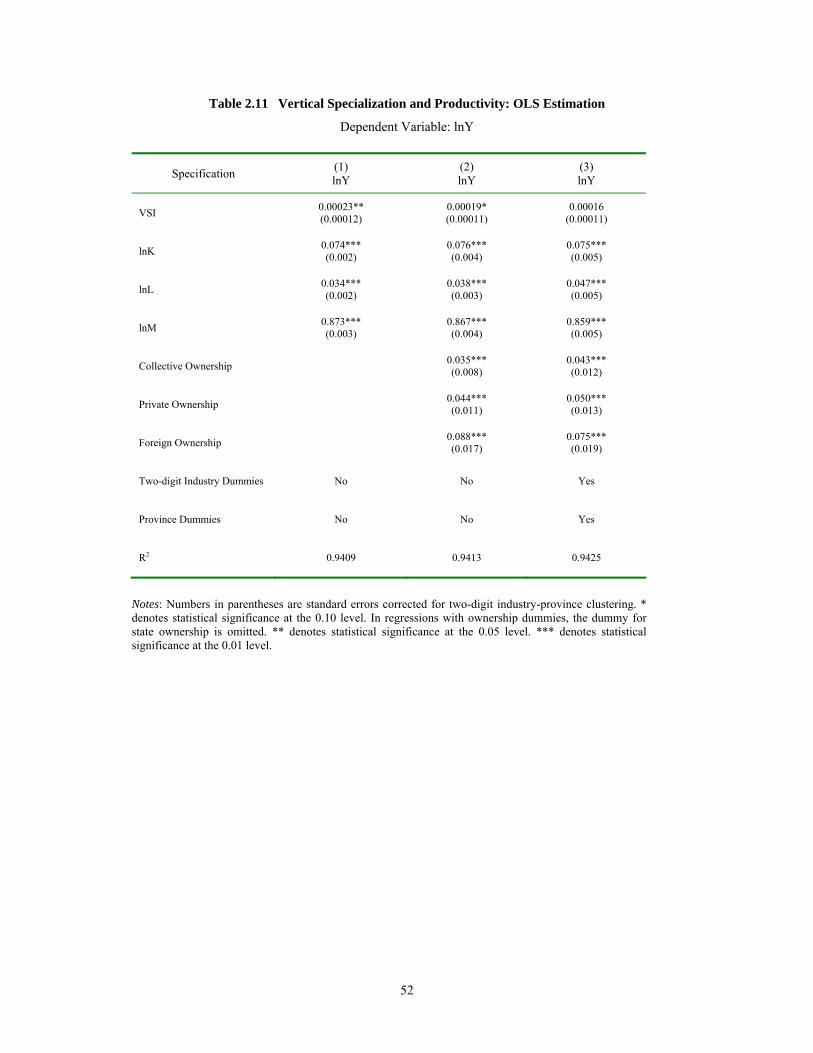
Table 2.11 Vertical Sp vity: OLS Estimation
Dependent Variable: lnY
Specification
ecialization and Producti
(1) lnY
(2) lnY
(3) lnY
VSI 0.00023** 0.00019* 0.00016 (0.00012) (0.00011) (0.00011)
lnK 0.074*** 0.076*** 0.075***
lnL 0.034*** 0.038*** 0.047***
lnM 0.873*** (0.003)
0.867*** 0.859***
Collective Ownership 0.035*** 0.043***
Private Ownership 0.044*** 0.050***
Foreign Ownership 0.088*** (0
0.075*** (0
Two-digit Industry Dummies No No Yes
Province Dummies No No Yes
R2 0.9409 0.9413 0.9425
(0.002) (0.004) (0.005)
(0.002) (0.003) (0.005)
(0.004) (0.005)
(0.008) (0.012)
(0.011) (0.013)
.017) .019)
Notes: Numbers in parentheses are standard errors corrected for two-digit industry-province clustering. * denotes statistical significance at the 0.10 level. In regressions with ownership dummies, the dummy for state ownership is omitted. ** denotes statistical significance at the 0.05 level. *** denotes statistical significance at the 0.01 level.
52

Table 2.12 Vertical Specializatio and Productivity: IV Estimation
Specification (1) (2) (3) (4) (5) (6)
n
Pa nd-S essi den : lnYnel A: Seco tage Regr on Depen t Variable
VSI 0.0012 0.0012 0.0012
0.101*** 0.050*** 0.097*** 0.048*** 0.100*** 0.049***
0.078*** 0.034*** 0.073*** 0.032*** 0.077*** 0.032**
lnM 0.801*** (0 )
0.928*** (
0.810*** (0 )
0.933*** (
0.805*** (0 )
0.930*** (
s No Yes No Yes No Yes
Two-digit Industry
No Yes No Yes No Yes
P-Value of Sargan test 0.4583 0.3985
Pa rst-St ssion dent VSI
-1.61*** -1.22*** -1.63*** -1.21*** -1.63*** -1.22***
lnL
lnM 4.21*** (0
3.53*** (0
0.55*** (0
0.27*** (0
0.34*** (
0.22*** (
0.17*** (
0.13*** (
s
Two-digit Industry No Yes No Yes No Yes
Province Dummies No Yes No Yes No Yes
R2 0.0697 0.1184 0.0696 0.1184 0.0697 0.1185
*** (0.0004)
0.0010** (0.0005)
*** (0.0004)
0.0010** (0.0005)
*** (0.0004)
0.0010** (0.0005)
lnK (0.013) (0.013) (0.012) (0.013) (0.012) (0.013)
lnL (0.013) (0.013) (0.019) (0.011) (0.019) (0.013)
.033 0.048) .030 0.046) .030 0.048)
Ownership Dummie
No Yes No Yes No Yes Dummies
Province Dummies
nel B: Fi age Regre Depen Variable:
lnK (0.04) (0.05) (0.04) (0.05) (0.05) (0.05)
-2.74*** (0.05)
-2.21*** (0.05)
-2.64*** (0.05)
-2.24*** (0.06)
2.71*** (0.05)
-2.25*** (0.06)
4.22*** (0.04)
3.46*** (0.04) .04) .05)
4.19*** (0.04)
3.56*** (0.05)
four-digit Industry Size .06) .05) 0.39*** (0.08)
0.19*** (0.06)
Three-digit Industry Size 0.04) 0.05) 0.04) 0.04)
Ownership Dummie No Yes No Yes No Yes
Dummies
Notes: Numbers in parentheses are standard errors corrected for two-digit industry-province clustering. * denotes statistical significance at the 0.10 level. ** denotes statistical significance at the 0.05 level. *** denotes statistical significance at the 0.01 level.
53

3. DO DOMESTIC FIRMS BENEFIT FROM FOREIGN DIRECT INVESTMENT?
THE CASE OF CHINA
3.1. Overview of FDI Spillover Channels
3.1.1. Horizontal Spillovers
Horizontal spillovers of FDI take place when the presence of FDI increases the productivity of
the domestic firms in the same industry. Teece (1977) argues that such spillovers can occur
through various channels. The first channel is the demonstration effect. Domestic firms may be
able to reduce the innovation costs simply by observing and imitating the foreign firms. The
second channel is labor turnover. Workers employed and trained by foreign firms may join
domestic firms or create their own firms. The third channel is the competition effect. The entry
of foreign firms can force domestic firms to restructure and improve their production techniques
and management.
However, the increased intensity of competition may hurt domestic firms at least in the
short run by reducing their market share and output. As shown by Aitken and Harrison (1999),
the productivity of domestic firms would fall if they have to spread their fixed costs over smaller
sales volume. This is usually interpreted as a crowding-out effect. The entry of foreign firms may
also raise labor costs of domestic firms. Since foreign firms often pay higher wages, they may
raise wages for all firms in competitive labor markets (Aitken, Harrison, and Lipsey, 1996).
Theoretically, the net horizontal effect of FDI on domestic firms is inconclusive.
54

There are two generations of empirical studies on horizontal effects. The first generation
is characterized by industry-level studies. A partial list includes Caves (1974) for Australia,
Globerman (1979) for Canada, and Blomstrom and Persson (1983) for Mexico. Most of the first
generation studies find a positive correlation between FDI and industry productivity. Since they
rely on cross-sectional data, it is difficult to distinguish whether FDI actually increases domestic
firms’ productivity, or whether foreign investors are simply attracted to high-productivity
industries.
The second generation of empirical studies is based on firm-level panel data. The
advantage of the panel data approach is that it can control for foreign investor selection bias.
These studies examine whether foreign presence increases the productivity of the firms in the
same industry. The results, however, have been mixed. In a study of Venezuelan factories,
Aitken and Harrison (1999) find net negative benefits to domestic firms, a result that they
attribute to the crowding-out effect. Other studies that find negative spillovers include Haddad
and Harrison (1993) for Morocco, Djankov and Hoekman (2000) for the Czech Republic,
Konings (2001) for Bulgaria, Romania, and Poland, and Javorcik (2004) for Lithuania. In
contrast, studies on developed countries often find evidence of positive spillovers. They include
Haskel, Pereira, and Slaughter (2002) for the United Kingdom, Keller and Yeaple (2003) for the
United States, Castellani and Zanfei (2002) for Italy, and Gorg and Strobl (2003) for Ireland.
In the case of China, Cheung and Lin (2003) find positive effects of FDI in China on the
number of patents by using a provincial panel dataset. Based on 1995 industrial census data in
China, Tong and Hu (2003) find significant horizontal spillovers from FDI.
55
3.1.2. Vertical Spillovers
Backward spillovers of FDI refer to the technology transfer through supply chains from
foreign firms to domestic suppliers. If foreign firms are successful at preventing the leakage of
their firm-specific knowledge to domestic competitors in the same industry, there is no scope for
intra-industry technology spillovers. It is possible, however, that foreign firms voluntarily or
involuntarily help increase efficiency of domestic suppliers through backward linkages. Foreign
firms can provide technical assistance, training and other help to their domestic suppliers in order
to improve the quality of intermediate purchases.
Similarly, forward spillovers occur when domestic firms gain access to new or less costly
intermediate inputs as a result of the foreign investment in upstream industries.
Evidence of technology transfer through vertical supply chains is well documented in
case studies. For example, Kenney and Florida (1993) and Macduffie and Helper (1997) provide
a rich description of technology transfer to U.S. parts suppliers following the entry of Japanese
car makers. Blalock (2002) analyzes Indonesian firms and Javorcik (2004) studies a panel dataset
from Lithuanian industries, both of which find positive FDI spillovers through backward
linkages. Using both industry level and firm level data, Liu and Lin (2004) find evidence of
backward spillovers in China.
3.1.3. Local Spillovers
Given that labor turnover and demonstration effect are among the most important channels for
technology spillovers, there are good reasons to expect that any benefits to the domestic firms
from foreign investment would be received primarily by the firms located nearby: (1) if a skilled
worker leaves a foreign firm to work for a domestic firm, he or she is likely to choose a firm in
56

the same region; (2) if a new technology or a new management technique is introduced by a
foreign firm, the domestic firms located close to it have an advantage over more distant firms in
observing and imitating the foreign firm. Of course, domestic firms that are closer to foreign
firms may also suffer more from the competition.
Note that if the workers’ skills, new technologies and management techniques are
transferable across industries, local spillovers may still occur even without direct horizontal or
vertical linkages between domestic and foreign firms.
In the case of China, the entry of FDI can facilitate the institutional changes and the
improvements in the legal system. Thus, a region with a longer history of FDI tends to have
better business environment. All these factors may contribute to improving the productivity of
local firms.
The geographic dimension of FDI spillovers has been investigated in a number of
empirical studies. Using cross-sectional data for Indonesia, Sjoholm (1999) finds no evidence for
local spillovers. Aitken and Harrison (1999) also fail to find positive spillovers from the foreign
firms to nearby domestic firms in Venezuela. From firm-level panel data, Girma and Wakelin
(2002) find evidence for positive spillovers from FDI in the same region and same industry in
United Kingdom.
3.2. Foreign Direct Investment in China
For the past 25 years, China has aggressively pursued policies that encourage FDI inflow.
For example, China developed the first law governing foreign investment in 1979, while the first
laws relevant to domestic firms were not enacted until 1988.
57

According to Chinese laws, foreign firms can invest in China through joint ventures,
cooperative enterprises, and solely owned enterprises. The establishment of solely foreign-owned
enterprises was subject to strict restrictions from Chinese government, such as export volume
and local procurement. These restrictions were removed in 2001 in accordance with WTO
framework. Consequently, solely foreign-owned enterprises became the most popular form of
FDI in post-WTO China.
Hong Kong is the most important source of FDI in China. In 2003, Hong Kong invested
17.7 billion dollars in China, accounting for 33 percent of the total.12 Other sources of FDI
include Japan, United States, South Korea, Taiwan and Virgin Islands.13 In recent years, an
increasing share of FDI came from global giants in industrialized countries such as Motorola,
SONY and Siemens.
Nearly 70 percent of FDI in China was poured into the manufacturing sector. This is
mainly due to the competitive edge of relatively low production cost in China for manufacturing.
The other reason is that FDI in service sector has not been fully liberalized.
The geographic distribution of FDI has been quite uneven. China initiated its “open door”
policy by establishing four special economic zones in 1980. In 1984, it further opened 14 coastal
cities. Then in the early 1990s, China expanded its open regions from the coastal cities to the
inland regions and from the east to the west. Due to their convenient location, better
infrastructure and legal environment, the coastal regions have been the main recipients of FDI in
China. For example, in 2003, the coastal provinces received 88 percent of the total FDI in China.
12 Part of the investment from Hong Kong is originated from Chinese firms who register in Hong Kong and re-enter China as “foreign investment.” This is often called “round-tripping.” 13 Many foreign firms, especially those from Taiwan and Hong Kong, invest in China via such international tax havens as Virgin Islands.
58

The contribution of foreign invested firms to China’s economy has been remarkable. FDI
accounted for about 9 percent of total investment in fixed assets, 31 percent of industrial output,
and 55 percent of foreign trade in 2003.14
When a foreign firm acquires a domestic firm or sets up a joint venture with a domestic
firm, it usually brings more advanced technology and managerial techniques to the new firm. In
a survey of 127 foreign invested firms by Jiang (2002), 65 percent of the firms adopted some
technology that filled in the technological gaps in China. In addition, in a transition economy like
China, foreign investment can facilitate the restructuring of state-owned enterprises by cutting
government-enterprise relation and hardening the budget constraint. For example, when foreign
investors join an existing firm, they usually demand that professional managers take over the
decision rights from government-appointed officials.
The technology spillovers from FDI to domestic firms can be found in mobile phone
industry. China’s domestic firms began to produce mobile phones in 1999. Driven by the rapid
growth of the market, domestic firms quickly improve their products by borrowing new
technology from foreign invested firms in China. In only a few years, their market share jumped
from 2 percent in 1999 to over 60 percent in 2003 (Long, 2005).
The foreign firms often develop close vertical relationships with Chinese firms. For
example, Motorola plant in Tianjin is supplied by about 80 supporting firms in Tianjin and 170
firms outside Tianjin. Most of them are domestic firms. Motorola often sends personnel to offer
technical guidance to these local suppliers.
14 Source: Author’s Calculation based on China Statistical Yearbook (2004).
59

3.3. Measurement and Data
3.3.1. Measuring Horizontal Spillovers
The variable, jtHorizontal , measures the foreign presence in the firm’s own industry j at time t. It
is calculated as follows:
,∑
∑
∈
∈
×
=
jiit
jiitit
jt Sales
SalesreForeignShaHorizontal (3.1)
where reoreignSha is define as the share of firm i’s total equity owned by foreigners. We
define the industry at the four-digit le
itF
vel.
3.3.2. Measuring Backward Spillovers
jtBackward captures the foreign presence in the downstream industries that are supplied by
industry j. Since the firm-level dataset does not provide information about backward linkage, we
use backward linkage values of the firm’s industry. In particular, we have
.∑≠ jk
jk
= ktjkjt HorizontalBackward α (3.2)
α is the proportion of industry j’s total output that is purchased by industry k. We exclude the
purchase by own industry because we have already included
15
its in the regression.
coefficient
jtHorizontal
he jkαT is calculated using the input-output table of 1997.
15 For example, suppose industry A sells 10% of its output to industry B, 30% to industry C and 60% to industry D, where Foreign Share is 30%, 20% and 25%, respectively. In this example, Backward of industry A = 0.1×0.3 + 0.3×0.2 + 0.6×0.25 = 0.24.
60

3.3.3. Measuring Forward Spillovers
Similarly, jtForward shows the foreign presenc stream industries from e in the up which industry
j purchas di ing way:
jkktjkjt
es its interme ate inputs. We calculate jtForward in the follow
.∑= HorizontalForward β (3.3) ≠
is the proportion of industry j’s intermediate inputs that is supplied by industry k. The jkβ
coefficient jkβ is calculated based on the input-output table of 1997.
is a proxy for foreign presence in region r. We define the region at city level (four-digit
3.3.4. Measuring Local Spillovers
rtLocal
geographic level). The computation of rtLocal is similar to jtHorizontal :
,∑
∑ ×=
it
itit
rt Sales
SalesreForeignShaLocal (3.4)
∈
∈
ri
ri
Tables 3.1-3.4 present basic information about these four spillover variables at the two-
digit industry level or at the provincial level. In all these variables, there is large variation across
industries or regions. For example, as can be seen from Table 3.1, in 2003 Horizontal ranges
from 0.2 percent in tobacco processing to 69.1 percent in electronics and telecommunications.
3.3.5. The Data and Basic Patterns
This empirical study is based on a large dataset of Chinese industrial firms built from cross-
sectional data collected in regular surveys by China National Bureau of Statistics between 2000
and 2003. The surveys cover all state-owned firms and all non-state firms above designated
61

scale. O
c information of each four-digit industry. The dataset contains detailed information of
about 1
out 60
percen
ID numbers
after re
Table 3.6 shows that in our dataset, foreign firms account for about 20 percent of total
nly non-state firms with sales under 5 million Yuan are excluded. The firms in our
sample accounted for about 65 percent of total industrial value added in 2000 (Table 3.5). This
share dropped to 53 percent in 2001 and rose to 72 percent and 79 percent in 2002 and 2003.
Since we only focus on manufacturing sector, the sample size decreases to 140,000 to
180,000 firms per year. The number of observations is further reduced by deleting those with
missing values and those that fail to satisfy some basic error checks. The industry section of
China Statistical Yearbook is complied based on this dataset. China Markets Yearbook reports
the basi
00 variables, including ID number, ownership, sales revenue, value added, four-digit
industry code, six-digit geographic code, exports, employment, capital stock, and intermediate
inputs.
We construct a panel dataset by matching the firms by their ID numbers. Only ab
t of the firms in the dataset can be matched throughout the entire period (four years). This
is because in addition to normal exit and entry, existing firms often change their
structuring, which significantly reduces the percentage of firms that we can match.
number of firms in each year. Summary statistics are reported in Tables 3.7 and 3.8.
To compare foreign firms with domestic firms, we estimate the following equation:
,ln 0 ijrii reForeignShaS εααβα +++∗+= (3.5)
where iS refers to firm i’s characteristics, including TFP, labor productivity defined as value-
added per worker, sales, employment, capital intensity, and wage. We estimate (3.5) separately
for each year in our sample. In the regression, we also control for two-digit industry and
provincial fixed effects.
62

The estimation results reported in Table 3.9 suggest that foreign firms differ significantly
from domestic firms. The estimated coefficient, β, has a clear economic interpretation, i.e., it
shows the percentage differential between a wholly foreign-owned firm and a domestic firm. For
example, in 2003, the TFP of a wholly foreign-owned firm was on average 40 percent higher
an that of a domestic firm. In general, foreign firms are larger, more productive, more capital
intensive, and pay higher wages. Our findings are consistent with previous studies on other
countries (e.g., Bellak, 2004)
3.4. Empirical Strategy
hip between FDI and the productivity of domestic firms, we follow an
oa that is commonly used in the literature (e.g., Aitken and Harrison, 1999). We estimate a
t n th t inclu illovers measures as explanatory variables. Our starting point
HorizontalreForeignShaKLY lnlnln
th
To investigate the relations
appr ch
production func io a des sp
is the following equation:
ijrtijrtijrtijrt 21210 jtγγββα ++++=
ijrtjrt 543 rtjtjt LocalForwardBackward ,γγγ ++++ εααα +++ (3.6)
where
ijrtY is the real value-added of firm i in industry j and region r at time t, which is deflated
by industry-specific ex-factory price index. ijrtL is the number of employees. ijrtK stands for the
net value of fixed assets deflated by investment price index.16
As an exploratory regression, (3.6) is estimated with OLS on the full sample and the
subsample of domestic firms only. Since the spillovers may take time to materialize, we also
16 According to China’s accounting practice, net value of fixed assets of year t = net value of fixed assets of year t-1 + investment of year t – depreciation of year t. To get net value of fixed assets of year t in constant price, ideally we should only deflate investment of year t. Since the price level was almost constant during 2000-2003, deflating net value of fixed assets by investment price index makes little difference.
63

estimate (3.6) with one-year lagged spillover variables. The model includes a full set of year,
two-digit industry, and provincial dummies. The results are reported in Table 3.10. The standard
errors reported throughout the chapter are corrected for two-digit industry-province clustering
oulton, 1990). In all cases, we find positive and statistically significant coefficients on
ble of Horizontal does not appear to be significant. The
ometric concerns with the estimation of (3.6). The first is the omission of
firm-sp
ent team.
O e solution to this problem is time differencing model. Following Haskel, Pereira, and
Slaughter (2002) and Javorcik (2004), instead of (3.6), we estimate the following first differences
(M
Backward and Local variables. The varia
coefficient on Forward is significant only when lagged values are used.
3.4.1. First Differences Estimation
There are two econ
ecific unobservable variables. These variables may affect the correlation between firm
productivity and FDI presence. Examples include government subsides or strong senior
managem
n
model:
jtijrtijrtijrtijrt HorizontalreForeignShaKLY ∆+∆+∆+∆=∆ 2121 lnlnln γγββ
3 Backwar ,54 ijrtjrtrtjtjt LocalForwardd εαααγγγ ++++∆+∆+ (3.7)
ince differencing also removes time, region and industry effects, unlike (3.6), year, region and
dustry dummies in (3.7) will control for unobservables that are related to the change in time,
∆+
S
in
region and industry effects.17
17 For example, we control not just for “Shanghai is an attractive city for foreign investment” but also for “the attraction of Shanghai for foreign investment changes over time.”
64

3.4.2. Semi-Parametric Estimation
The second econometric problem is that OLS is biased when estimating the production function
in (3.6) because labor and intermediate inputs are not exogenous. Griliches and Mairesse (1998)
argue that inputs should be endogenous since they are chosen by firms after productivity is
observed. To correct the endogeneity bias, Olley and Pakes (1996) propose a semi-parametric
estimation procedure that uses investment as a proxy for the unobservable productivity shock.
Since t
cedure can avoid this problem because usually
the inte
h the Levinsohn-Petrin procedure does not account
for sele
) and Levinsohn and Petrin (2003) find that controlling for selection has
little effect on the final parameter estimates.
he Olley-Pakes procedure requires the information of investment which is not available in
our dataset,18 we opt for the Levinsohn and Petrin (2003) procedure, which uses intermediate
inputs rather than investment to address the underlying endogeneity issues.
There are two advantages for the Levinsohn-Petrin procedure. First, because there is
substantial adjustment cost with capital stock, in many firm-level datasets, a large number of
observations have zero investment. These observations must be deleted to satisfy the strict
monotonicity condition. The Levinsohn-Petrin pro
rmediate inputs must be positive. Second, intermediate inputs provide a better proxy for
productivity shock than investment because investment does not respond to the productivity
shock quickly enough due to the adjustment cost.
The advantage of the Olley-Pakes method is that the original three-stage procedure
explicitly controls for selection bias. Althoug
ction bias, the authors argue that the use of unbalanced panel minimizes such bias. Both
Olley and Pakes (1996
18 In our dataset, the investment in year t can be calculated as the difference in the original value of fixed assets between year t and year t - 1, but we will lose one year data, leaving only three years in our panel.
65

To briefly discuss the consider the following
io u 20
Levinsohn-Petrin procedure,19 let us
product n f nction:
,0 ititkitlit ly it ηωββββ ++++= (3.8)
where ity , itl , and itk denote logarithms of value-added, labor and capital. Note that the error
term has two components: (1) productivity shock, itω ; (2) the error term that is uncorrelated with
input choices, itη . In t equa onhe ti , itω is a state variable and affects the input decision.
Levinsohn and Petrin assume that demand for
firm’s
the intermediate inputs depends on the
state variables itk and itω :
).,( itititit kmm ω= (3.9)
Levinsohn and Petrin show that the dem nd a function is monotonically increasing in itω .
It is possible to invert the intermediate input dem
productivity shock
and function and express the unobserved
as a function of and : itk itmitω
).,( ititit mkωω = (3.10)
A further assumption follows Olley and Pakes (1996). Levinsohn and Petrin assume that
the productivity shock follows a first-order Markov process:
[ ] ,| 1 itititit E ξωωω += − (3.11)
where itξ is a change in productivity uncorrelated with .
Equation (3.8) can now be rewritten as
itk
.),( ititititlit mkly ηφβ ++= (3.12)
19 For complete exposition of the procedure, please refer to Levinsohn and Petrin (2003). 20 There are two versions of Levinsohn-Petrin procedure: one based on revenue and one based on value-added. In the former case, revenue is a function of labor, capital and intermediate inputs. When revenue is used, Levinsohn-Petrin procedure requires GMM estimation in the second stage. The coefficients will only be weakly identified in GMM estimation with our data because we have a relatively short panel (only four years). Thus the version of value-added is chosen in this study.
66

where ),(),( 0 itititkitit mkkmk ωββφ ++= .
By substituting a third-order polynomial approximation in and for itk itm ),( itit mkφ , it is
possibl
3 pqpmkly ηδβδ +++= ∑∑
−
(3.13)
Therefore, we can obtain consistent estimates of
e to consistently estimate (3.12) using OLS as
.3
0 00 it
p qititpqitlit
= =
lβ and itφ , which completes the first
stage of the procedure.
In the second stage, we first compute the estimated value for itφ using
itlitit ly βφ ˆˆˆ −=
3 3 p−
.ˆˆˆ0 0p q= =
0 itlqit
pitpq lmk βδδ −+= ∑∑ (3.14)
For any candidate values *kβ , we can compute a prediction for itω for all periods t, since
. Using these predicted values, a consistent ap ation to itEitkitit k*ˆˆ βφω −= proxim | −it[ ]1ωω ,
[ ]1|ˆ−ititE ω , is given by the predicted values from tω he regression
(3.15)
c puted as
.ˆ 313
212110 ititititit εωγωγωγγω ++++= −−−
It then follows that the sample residual of the production function can be om
[ ].|ˆˆ1
*−−−−=+ itititkitlititit Ekly ωωββξη . (3.16)
The estimate kβ̂ is defined as the solution to
[ ]( ).|ˆˆ *∑ −−−t
Eklyk
ωωβββ
min 1−itititkitlit (3.17)
A bootstrap approach is used to . calculate the standard errors for lβ̂ and β̂k
67

The Levinsohn-Petrin procedure is implemented in this dissertation using the Stata
module “levpet” developed by Petrin, Levinsohn and Poi (2004).
We perform the Levinsohn-Petrin procedure for each two-digit industry separately. The
measure of lnTFP is calculated as follows:
milar results. The size of the
coefficients does not ch
deviation (5 percentage points) increase in the foreign presence in the downstream industries is
associated with 3.2 percent increase in TFP of the domestic firms in the supplying industry. A
.itkitlitit klyTFP ββ +−= (3.18)
3.5. Estimation Results
3.5.1. Baseline Specifications
The estimation of the first differences model, Equation (3.7), produces findings of
backward spillovers and local spillovers. The first two columns of Table 3.11 present the
estimation results for all firms (full sample) and the subsample of domestic firms, respectively.
In both cases, the coefficients on backward spillovers and local spillovers appear to be positive
and statistically significant. The third and fourth columns report the results from the regressions
with ∆lnTFP, which is calculated through the Levinsohn-Petrin procedure. Again positive and
significant coefficients on backward spillovers and local spillovers can be found for both the full
sample and the subsample of domestic firms. As shown by the last two columns of Table 3.11,
the regressions with labor productivity produce qualitatively si
ˆˆln
ange very much across specifications. In the case of domestic firms, the
coefficient on backward spillovers is larger while the coefficient on local spillovers is smaller.
The backward and local spillover effects are also quantitatively significant. A one-standard-
68

one-standard-deviation (13 percentage points) increase in the foreign presence in a city raises the
TFP of the domestic firms in the same city by 4 percent.21
rted in Table 3.12. A positive and significant coefficient on backward
illovers can be found in all regressions except in the case of labor productivity for the
pl e of local spillovers has a significantly positive
s not clear which types of foreign firms are more
likely to generate spillovers to domestic firms. Hong Kong, Macao and Taiwan are among newly
Little evidence can be found for other channels of spillovers. In most cases, the
coefficient on the horizontal spillovers bears a negative sign but appears statistically
insignificant. This finding is consistent with previous research that generally fails to find positive
horizontal spillovers in developing countries. The variable of forward spillovers has a positive
sign but it is not statistically significant.
In order to check the robustness of the results, we estimate a model in second differences.
The main cost of differencing is that it can aggravate measurement error in the independent
variables. Longer time differences tend to attenuate this problem (Griliches and Hausman, 1986)
but they also reduce the sample size. The estimation results of the regressions with second
differences are repo
sp
subsam e of domestic firms. The variabl
coefficient in all cases, although the size of the coefficient is smaller compared to first
differences. There is no robust evidence of horizontal and forward spillovers in the model of
second differences.
3.5.2. HMT firms versus OECD firms
Chinese statistics identify two types of foreign invested firms in China: those invested by
overseas Chinese from Hong Kong, Macao and Taiwan (HMT), and those invested by foreign
investors mainly from OECD countries. It i
21 The calculation is based on the fourth column of Table 3.10.
69

industr
ized brand names.
.22 We find robust evidence of backward spillovers and local spillovers from both
MT and OECD firms, which is consistent with our previous findings. The size of the
aller in the case of OECD firms, indicating that these firms rely
to domestic firms are only generated if the technology
gap be
ialized economies. The investors from these regions have additional advantages of same
culture, same language, geographical proximity, or even family ties. Compared with HMT firms,
the advantages of OECD firms lie in their more advanced technology, global production chain
and internationally recogn
To investigate whether there exist different impacts of HMT and OECD firms, we
estimate (3.7) separately for these two types of firms. Spillover variables are constructed using a
new modified Foreign Share variable, which is now defined as the share of firm’s equity owned
by HMT (OECD) firms.
The results from the regressions with the subsample of domestic firms are reported in
Table 3.13
H
coefficient on Backward is sm
more on their own global supply chain. There is little evidence of spillovers through other
channels.
3.5.3. Technological Gap
Recent studies on FDI find that horizontal spillovers depend on the absorptive capacity of the
domestic firms. If the technological gap between foreign and domestic firms is large, domestic
firms may lack the ability needed to adopt the new technology. Borensztein, Gregorio and Lee
(1998) argue that positive FDI spillovers
tween the foreign firms and the domestic firm is not too wide. Using a cross-section of
firm-level data for Uruguay, Kokko, Tansini, and Zejan (1996) find evidence for productivity
22 There is no big difference between the results from the full sample and the subsample. Since we are more interested in the spillover effects on domestic firms, we only report the results using the subsample of domestic firms.
70

spillovers to domestic firms with moderate technological gaps, but not for firms that use
considerably lower levels of technology.
Technological gap can also be important for vertical spillovers. Even if the foreign firms
outsour
to local
supplie
ne
ecification. In most cases, the coefficients on Backward and Local have positive signs and are
rizontal is negative and
international markets tend to put less pressure on domestic competitors. Second,
export-
ce locally, their local suppliers may fail to learn and absorb the technology transferred if
they are far behind their foreign partners in productivity (Smarzynska, 2002). Thus absorptive
capacity of local supplier is an important factors driving technology transfer from FDI
rs.
We reestimate the first differences model with the subsample of the most productive
domestic firms. For each two-digit industry, we select those domestic firms whose average TFP
over the period 2000-2003 falls into top 25 percent of all domestic firms in that industry.
The results shown in Table 3.14 exhibit patterns that are similar to the baseli
sp
statistically significant. A notable difference is that the coefficient on Ho
statistically significant in the cases of TFP and labor productivity. This finding is consistent with
the observation that foreign firms are often competing head-to-head with elite domestic firms.
3.5.4. Export-Oriented versus Domestic-Market-Oriented FDI
It has been suggested that the market orientation of the foreign firms is likely to affect both
horizontal and vertical spillovers (Sgard, 2001; Javorcik, 2004). First, domestic-market-oriented
foreign firms take market share directly from domestic firms, while export-oriented foreign firms
that target
oriented foreign firms are often part of global production network. They usually depend
on the suppliers from their parent company or their affiliates in other countries. Therefore,
71

export-oriented foreign firms are more likely to generate horizontal spillovers but not backward
spillovers.
To test this hypothesis, we estimate (3.7) using only export-oriented foreign firms as our
measure of foreign presence. In our dataset, about 70 percent of foreign firms were engaged in
exports between 2000 and 2003. Export-oriented firms are defined as those firms that exported
90 percent of their production.
The estimation results in the last three columns of Table 3.14 indicate that in terms of
ductivity spillovers, export-oriented foreign firms are not very different from domestic-
market-oriented foreign firms. Again we find the same positive backward and local spillovers.
The coefficient on Horizontal turns positive but remains statistically insignificant.
pro
72

Table 3.1 Horizontal Spillover Variable by Two-Digit Industry Unit: %
Code Industry 2000 2001 2002 2003 6 Coal Mining & Processing 1.0 0.7 0.6 0.6 7 Petroleum & Natural Gas Extraction 2.3 7.2 6.8 5.7 8 Ferrous Metals Mining & Processing 1.2 0.8 0.9 0.7 9 Non-Ferrous Metals Mining & Processing 1.2 1.1 1.4 1.3 10 Nonmetal Minerals Mining & Processing 4.6 4.3 4.1 4.6 13 Food Processing 0.0 0.0 0.0 0.8 14 Food Production 17.8 17.3 18.7 19.1 15 Beverage Production 31.4 34.3 30.2 31.9 16 Tobacco Processing 23.6 24.4 26.1 27.3 17 Textile 0.2 0.2 0.2 0.2 18 Garments & Other Fiber Products 15.3 16.4 16.7 17.9 19 Leather, Fur, Feather and Related Products 36.0 36.0 35.1 36.5 20 Timber Processing, Bamboo, Cane &Palm 44.9 42.6 41.5 40.6 21 Furniture Manufacturing 21.3 22.1 21.0 20.9 22 Papermaking & Paper Products 36.3 37.0 37.1 42.8 23 Printing, Reproduction of Recording Media 24.0 25.5 25.5 25.3 24 Stationery, Educational & Sports Goods 20.8 23.9 23.2 24.6 25 Petroleum Processing, Coking Products, & Gas 51.2 50.9 51.6 52.0 26 Raw Chemical Materials & Chemical Products 4.7 6.6 7.6 6.9 27 Medical & Pharmaceutical Products 15.3 16.6 17.3 19.1 28 Chemical Fibers 16.5 15.4 15.1 15.4 29 Rubber Products 23.2 18.7 18.5 15.3 30 Plastic Products 26.7 27.4 29.3 29.6 31 Nonmetal Mineral Products 35.3 34.5 33.1 35.0 32 Smelting & Pressing of Ferrous Metals 12.9 13.7 13.5 12.1 33 Smelting & Pressing of Non-Ferrous Metals 4.9 6.0 6.4 7.4 34 Metal Products 8.3 8.2 8.2 8.8 35 General Machinery & Equipment Manufacturing 28.8 27.4 27.6 26.8 36 Special Machinery & Equipment Manufacturing 17.3 17.1 17.7 19.5 37 Transportation Equipment Manufacturing 11.8 14.6 15.1 15.9 40 Electric Equipment & Machinery 19.1 20.3 19.0 21.9 41 Electronic & Telecommunications 27.7 28.1 28.1 29.0 42 Instruments, Meters, Cultural & Office Equipment 56.2 59.7 63.1 69.1 43 Manufacture of Artwork and Other Manufacturing 51.4 53.4 55.5 61.5 44 Production and Distribution of Electric Power and Heat 35.0 35.1 35.3 32.8 45 Production and Distribution of Gas 4.5 4.6 4.5 4.4 46 Production and Distribution of Water 11.3 11.1 15.9 20.9
Note: See Section 3.3 for the definition of the horizontal spillover variable. Source: Author’s calculation based on the database.
73

Table 3.2 Backward Spillover Variable by Two-Digit Industry Unit: %
Code Industry 2000 2001 2002 2003 6 Coal Mining & Processing 10.3 10.7 10.1 10.4 7 Petroleum & Natural Gas Extraction 4.7 5.4 6.6 6.1 8 Ferrous Metals Mining & Processing 9.7 9.7 10.0 10.6 9 Non-Ferrous Metals Mining & Processing 9.7 9.7 10.0 10.6 10 Nonmetal Minerals Mining & Processing 14.7 15.3 14.6 15.2 13 Food Processing 31.2 30.3 28.6 29.5 14 Food Production 31.2 30.3 28.6 29.5 15 Beverage Production 31.2 30.3 28.6 29.5 16 Tobacco Processing 31.2 30.3 28.6 29.5 17 Textile 33.4 32.9 31.2 32.1 18 Garments & Other Fiber Products 19.2 20.2 19.4 20.3 19 Leather, Fur, Feather and Related Products 19.2 20.2 19.4 20.3 20 Timber Processing, Bamboo, Cane &Palm 23.3 23.9 23.0 23.8 21 Furniture Manufacturing 23.3 23.9 23.0 23.8 22 Papermaking & Paper Products 21.7 22.4 21.5 22.7 23 Printing, Reproduction of Recording Media 21.7 22.4 21.5 22.7 24 Stationery, Educational & Sports Goods 21.7 22.4 21.5 22.7 25 Petroleum Processing, Coking Products, & Gas 13.1 13.4 12.8 13.3 26 Raw Chemical Materials & Chemical Products 23.9 25.0 24.2 25.5 27 Medical & Pharmaceutical Products 23.9 25.0 24.2 25.5 28 Chemical Fibers 23.9 25.0 24.2 25.5 29 Rubber Products 23.9 25.0 24.2 25.5 30 Plastic Products 23.9 25.0 24.2 25.5 31 Nonmetal Mineral Products 23.3 24.5 24.0 25.9 32 Smelting & Pressing of Ferrous Metals 23.7 23.9 23.1 23.9 33 Smelting & Pressing of Non-Ferrous Metals 23.7 23.9 23.1 23.9 34 Metal Products 21.5 22.6 21.8 23.0 35 General Machinery & Equipment Manufacturing 15.9 16.3 15.1 15.6 36 Special Machinery & Equipment Manufacturing 15.9 16.3 15.1 15.6 37 Transportation Equipment Manufacturing 14.7 15.2 14.8 15.4 40 Electric Equipment & Machinery 24.7 27.0 26.3 28.9 41 Electronic & Telecommunications 26.3 27.2 26.5 28.3 42 Instruments, Meters, Cultural & Office Equipment 15.2 15.7 15.0 15.6 43 Manufacture of Artwork and Other Manufacturing 19.5 20.2 19.5 20.5 44 Production and Distribution of Electric Power and Heat 15.2 15.5 15.0 15.6 45 Production and Distribution of Gas 15.5 15.8 15.4 16.2 46 Production and Distribution of Water 17.2 17.7 17.0 17.7
Note: See Section 3.3 for the definition of the backward spillover variable. Source: Author’s calculation based on the database and 1997 input-output table.
74

Table 3.3 Forward Spillover Variable by Two-Digit Industry Unit: %
Code Industry 2000 2001 2002 2003 6 Coal Mining & Processing 14.9 15.1 14.6 15.1 7 Petroleum & Natural Gas Extraction 17.2 17.8 17.2 17.9 8 Ferrous Metals Mining & Processing 15.8 16.1 15.3 15.8 9 Non-Ferrous Metals Mining & Processing 15.8 16.1 15.3 15.8 10 Nonmetal Minerals Mining & Processing 15.1 15.6 14.7 15.2 13 Food Processing 20.7 21.3 20.3 20.8 14 Food Production 20.7 21.3 20.3 20.8 15 Beverage Production 20.7 21.3 20.3 20.8 16 Tobacco Processing 20.7 21.3 20.3 20.8 17 Textile 19.9 20.0 18.7 19.5 18 Garments & Other Fiber Products 17.0 18.1 17.6 18.5 19 Leather, Fur, Feather and Related Products 17.0 18.1 17.6 18.5 20 Timber Processing, Bamboo, Cane &Palm 18.5 18.7 18.0 18.6 21 Furniture Manufacturing 18.5 18.7 18.0 18.6 22 Papermaking & Paper Products 20.1 20.6 19.7 20.6 23 Printing, Reproduction of Recording Media 20.1 20.6 19.7 20.6 24 Stationery, Educational & Sports Goods 20.1 20.6 19.7 20.6 25 Petroleum Processing, Coking Products, & Gas 2.8 3.3 3.7 3.3 26 Raw Chemical Materials & Chemical Products 12.5 13.2 12.8 13.1 27 Medical & Pharmaceutical Products 12.5 13.2 12.8 13.1 28 Chemical Fibers 12.5 13.2 12.8 13.1 29 Rubber Products 12.5 13.2 12.8 13.1 30 Plastic Products 12.5 13.2 12.8 13.1 31 Nonmetal Mineral Products 13.9 14.3 13.7 14.0 32 Smelting & Pressing of Ferrous Metals 8.7 9.0 8.7 8.9 33 Smelting & Pressing of Non-Ferrous Metals 8.7 9.0 8.7 8.9 34 Metal Products 9.3 9.6 9.7 10.3 35 General Machinery & Equipment Manufacturing 16.7 17.0 16.9 17.9 36 Special Machinery & Equipment Manufacturing 16.7 17.0 16.9 17.9 37 Transportation Equipment Manufacturing 16.4 16.9 16.5 17.3 40 Electric Equipment & Machinery 17.6 18.1 17.7 18.9 41 Electronic & Telecommunications 21.6 21.7 21.1 21.9 42 Instruments, Meters, Cultural & Office Equipment 28.9 30.9 30.6 33.3 43 Manufacture of Artwork and Other Manufacturing 18.6 19.0 18.4 19.1 44 Production and Distribution of Electric Power and Heat 10.2 10.8 10.7 11.2 45 Production and Distribution of Gas 5.4 5.9 5.8 5.8 46 Production and Distribution of Water 13.0 13.2 12.3 12.6
Note: See Section 3.3 for the definition of the forward spillover variable. Source: Author’s calculation based on the database and 1997 input-output table.
75

Table 3.4 Local Spillover Variable by Province Unit: %
Rank in 2003 Region 2000 2001 2002 2003
1 Guangdong 44.7 49.4 50.7 55.1 2 Fujian 47.8 49.5 46.8 46.9 3 Shanghai 34.2 35.3 37.7 45.0 4 Tianjin 33.7 40.1 28.8 37.8 5 Jiangsu 21.8 23.4 25.2 28.4 6 Beijing 16.2 29.9 25.5 26.9 7 Liaoning 15.5 15.3 16.0 16.1 8 Zhejiang 13.9 14.4 12.8 12.8 9 Hainan 17.3 14.1 12.3 12.3 10 Chongqing 10.9 10.8 10.4 12.1 11 Guangxi 7.5 9.0 11.6 12.0 12 Shandong 11.4 10.5 9.7 9.7 13 Anhui 8.6 10.9 10.2 9.5 14 Hebei 6.8 6.3 6.5 7.6 15 Hubei 6.0 6.3 6.7 7.5 16 Inner Mongolia 4.3 4.9 6.6 17 Hunan 6.2 5.7 5.5 5.7 18 Jilin 10.9 4.6 5.3 19 Sichuan 4.5 4.8 5.1 5.1 20 Jiangxi 5.2 6.0 4.1 4.4 21 Xinjiang 1.0 0.7 2.8 4.2 22 Guizhou 4.0 3.7 4.5 4.1 23 Henan 5.1 3.7 3.7 3.8 24 Ningxia 3.3 2.9 3.0 3.8 25 Shaanxi 3.4 4.3 3.4 3.4 26 Heilongjiang 2.3 2.7 2.9 3.2 27 Shanxi 2.1 2.5 2.3 2.8 28 Yunnan 1.6 1.7 2.4 1.9 29 Qinghai 1.2 0.4 1.1 1.8 30 Gansu 0.9 1.8 1.9 1.5 31 Tibet 0.7 0.1 0.1 0.1
Note: See Section 3.3 for the definition of the local spillover variable. Source: Author’s calculation based on the database.
76

Table 3.5 Coverage of the Database
Unit: Trillion Yuan
(a) Value Added of All Firms in the Database (b) GDP of Industrial Sector (a)/(b)
2000 2.54 3.90 0.65
2001 2.23 4.24 0.53
2002 3.30 4.60 0.72
2003 4.20 5.31 0.79
Source: Figures of GDP of industrial sector are from China Statistical Yearbook (2004), Table 3-1.
Table 3.6 Number of Foreign Firms in the Database
2000 2001 2002 2003
Total Number of Firms 129,432 131,631 157,687 178,044
Total Number of Foreign Firms 26,965 28,327 32,766 37,443
─ HMT Firms 15,677 16,375 18,056 20,520
─ OECD Firms 12,499 13,281 16,452 18,677
Source: China National Statistical Bureau Enterprise Database. HMT firms are partly or fully funded by investors
from Hong Kong, Macao and Taiwan. OECD firms are partly or fully funded by investors from OECD countries.
77

Table 3.7 Summary Statistics
Summary Statistics for Levels
__________________________________
Summary Statistics for First Differences _________________________________
Number of Observations Mean Standard
Deviation Number of
Observations Mean Standard Deviation
lnY 548,421 8.3536 1.4526 290,122 0.1330 0.9701
lnL 548,421 8.2685 1.7035 290,122 0.0559 0.6465
lnK 548,421 4.8865 1.1321 290,122 0.0151 0.4263
ln(Foreign Share) 545,076 0.1553 0.3297 287,511 0.0015 0.1192
Horizontal 548,421 0.2349 0.1647 290,122 0.0040 0.0608
Backward 548,421 0.2352 0.0503 290,122 0.0032 0.0150
Forward 548,421 0.1661 0.0408 290,122 0.0023 0.0113
Local 548,421 0.2000 0.1890 290,122 0.0078 0.0355
Source: Author’s calculation based on the database.
78

Table 3.8 Additional Summary Statistics of Spillover Variables
Horizontal ______________________
Backward ______________________
Forward ______________________
Local ______________________
Year
Number of
Industries Mean St.
Dev.
Number of
Industries Mean St.
Dev.
Number of
Industries Mean St.
Dev. Number of Cities Mean St.
Dev.
2000 520 0.2204 0.1889 29 0.2294 0.0526 29 0.1641 0.0521 364 0.0870 0.1285
2001 521 0.2300 0.1947 29 0.2348 0.0495 29 0.1698 0.0535 357 0.0799 0.1298
2002 530 0.2235 0.1882 29 0.2252 0.0471 29 0.1643 0.0512 351 0.0821 0.1298
2003 525 0.2245 0.1915 29 0.2357 0.0496 29 0.1710 0.0554 351 0.0855 0.1342
Source: Author’s calculation based on the database.
Table 3.9 Firm Differentials of Characteristics between Foreign and Domestic Firms
2000 2001 2002 2003
lnTFP 0.5477 (0.0374)
0.6220 (0.0301)
0.4596 (0.0239)
0.3959 (0.0230)
ln(Value Added per Worker) 0.4570 (0.0638)
0.4904 (0.0507)
0.2919 (0.0412)
0.1804 (0.0398)
ln(Sales) 0.8216 (0.0369)
0.7440 (0.0301)
0.6953 (0.0432)
0.6657 (0.0261)
ln(Employment) 0.2957 (0.0386)
0.3518 (0.0349)
0.3890 (0.0340)
0.4419 (0.0326)
ln(Captial per Worker) 0.7368 (0.0601)
0.7221 (0.0510)
0.6545 (0.0432)
0.5798 (0.0396)
ln(Wage per Worker) 0.4411 (0.0295)
0.4068 (0.0246)
0.3819 (0.0277)
0.3503 (0.0188)
Number of Observations 128,589 130,747 156,450 176,768
Notes: All coefficients are significant at the 1% level. All regressions include a full set of two-digit industry, ownership and provincial dummies. Numbers in parentheses are standard errors corrected for two-digit industry-province clustering.
79

Table 3.10 OLS with Lagged and Contemporaneous Spillover Variables
Dependent Variable: lnY
Contemporaneous Spillover variables
____________________________
Lagged Spillovers Variables
_____________________________
All Firms Domestic Firms All Firms Domestic Firms
lnK 0.2522*** (0.0035)
0.2219*** (0.0040)
0.2661*** (0.0042)
0.2312*** (0.0048)
lnL 0.5454*** (0.0064)
0.5625*** (0.0072)
0.5650*** (0.0073)
0.5909*** (0.0084)
Foreign Share 0.2353*** (0.0279) 0.2468***
(0.0293)
Horizontal 0.0589 (0.0387)
0.0305 (0.0451)
Horizontal Lagged 0.0365
(0.0404) 0.0353
(0.0575)
Backward 1.3673** (0.6455)
1.6190** (0.6840)
Backward Lagged 1.0736***
(0.3012) 1.1630*** (0.3580)
Forward 1.3722 (1.3417)
1.5139 (1.3662)
Forward Lagged 0.4894* (0.2845)
0.8733** (0.3548)
Local 0.1209*** (0.0395)
0.1598*** (0.0457)
Local Lagged 0.1877*** (0.0494)
0.1689*** (0.0575)
Number of Observations 545,076 425,462 288,743 218,864
R2 0.9319 0.9241 0.9379 0.9354
Notes: All regressions include time dummies, two-digit industry dummies and provincial dummies. Numbers in parentheses are standard errors corrected for two-digit industry-province clustering. * denotes statistical significance at the 0.10 level. ** denotes statistical significance at the 0.05 level. *** denotes statistical significance at the 0.01 level.
80

Table 3.11 Regression in First Differences: Baseline Specifications
∆lnY ____ _________________
∆ln(TFP)
____ _________________
∆ln(Labor Productivity)
____ _________________
All Firms Domestic Firms All Firms Domestic
Firms All Firms Domestic Firms
∆lnK 0.0854*** (0.0040)
0.0827 (0.0041)
∆lnL 0.3038*** (0.0082)
0.2913 (0.0091)
∆Foreign Share
0.1143* (0.0604) 0.1256**
(0.0608) 0.0356 (0.0668)
∆Horizontal -0.0014 (0.0354)
-0.0435 (0.0396)
-0.0033 (0.0352)
-0.0459 (0.0395)
0.0115 (0.0380)
-0.0264 (0.0424)
∆Backward 0.6322** (0.3128)
0.8149** (0.3532)
0.6448** (0.3103)
0.8189** (0.3501)
0.5347* (0.3201)
0.7457** (0.3754)
∆Forward 0.1571 (0.2416)
0.0413 (0.2862)
0.1685 (0.2370)
0.0514 (0.2818)
0.1411 (0.2710)
0.0721 (0.3214)
∆Local 0.3949*** (0.1038)
0.2971** (0.1181)
0.3975*** (0.1027)
0.2917** (0.1170)
0.4153*** (0.1139)
0.3296** (0.1297)
Number of Observations 287,511 218,864 287,511 218,864 287,511 218,864
R2 0.12 0.13 0.10 0.11 0.09 0.10
Notes: All regressions include time dummies, two-digit industry dummies and provincial dummies. Numbers in parentheses are standard errors corrected for two-digit industry-province clustering. * denotes statistical significance at the 0.10 level. ** denotes statistical significance at the 0.05 level. *** denotes statistical significance at the 0.01 level.
81

Table 3.12 Regression in Second Differences: Baseline Specifications
∆lnY ____ _________________
∆ln(TFP)
____ _________________
∆ln(Labor Productivity)
____ _________________
All Firms Domestic Firms All Firms Domestic
Firms All Firms Domestic Firms
∆lnK 0.1169*** (0.0049)
0.1118*** (0.0054)
∆lnL 0.4216*** (0.0093)
0.4072*** (0.0098)
∆Foreign Share
0.3408*** (0.0996) 0.3358***
(0.0965) 0.3127*** (0.1056)
∆Horizontal -0.0759 (0.0594)
-0.1185* (0.0654)
-0.0796 (0.0589)
-0.1174* (0.0648)
-0.0659 (0.0639)
-0.0832 (0.0745)
∆Backward 0.3689* (0.2072)
0.5861** (0.2664)
0.3765** (0.1910)
0.5979** (0.2608)
0.3587* (0.2084)
0.4595 (0.3321)
∆Forward -0.0822 (0.4063)
0.0014 (0.4219)
-0.0871 (0.4159)
0.0023 (0.4394)
-0.0736 (0.3689)
0.0036 (0.4398)
∆Local 0.1346** (0.0635)
0.1548** (0.0731)
0.1456** (0.0677)
0.1626** (0.0730)
0.1226* (0.0705)
0.1775* (0.0986)
Number of Observations 141,516 104,698 141,516 104,698 141,516 104,698
R2 0.12 0.14 0.09 0.10 0.06 0.07
Notes: All regressions include time dummies, two-digit industry dummies and provincial dummies. Numbers in parentheses are standard errors corrected for two-digit industry-province clustering. * denotes statistical significance at the 0.10 level. ** denotes statistical significance at the 0.05 level. *** denotes statistical significance at the 0.01 level.
82

Table 3.13 Regression in First Differences: Robustness Checks
Spillovers from HMT FDI ____________________________________
Spillovers from OECD FDI
____________________________________
∆lnY ∆ln(TFP) ∆ln(Labor Productivity) ∆lnY ∆ln(TFP) ∆ln(Labor
Productivity)
∆lnK 0.0840*** (0.0041) 0.0839***
(0.0039)
∆lnL 0.2994*** (0.0090) 0.2971***
(0.0083)
∆Horizontal 0.0313 (0.0447)
0.0326 (0.0424)
0.0445 (0.0538)
-0.1006* (0.0593)
-0.1192 (0.0757)
-0.0674 (0.0764)
∆Backward 0.9171** (0.4497)
0.9090** (0.4332)
0.8116* (0.4505)
0.3304 (0.2065)
0.3419* (0.1987)
0.4904** (0.2071)
∆Forward 0.0241 (0.0417)
0.0195 (0.0388)
0.0124 (0.0488)
-0.2598 (0.2564)
-0.2651 (0.2521)
-0.2194 (0.2851)
∆Local 0.2925*** (0.0962)
0.3007*** (0.0978)
0.2958** (0.1278)
0.2187** (0.1094)
0.2209** (0.0995)
0.3210*** (0.1202)
Number of Observations 255,875 255,875 255,875 250,401 250,401 250,401
R2 0.12 0.10 0.10 0.12 0.12 0.10
Notes: We only report the results from the subsample of the domestic firms. All regressions include time dummies, two-digit industry dummies and provincial dummies. Numbers in parentheses are standard errors corrected for two-digit industry-province clustering. * denotes statistical significance at the 0.10 level. ** denotes statistical significance at the 0.05 level. *** denotes statistical significance at the 0.01 level.
83
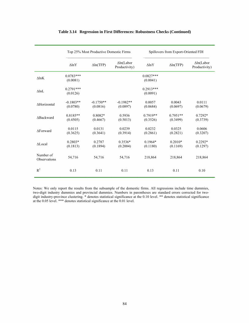
Table 3.14 Regression in First Differences: Robustness Checks (Continued)
Top 25% Most Productive Domestic Firms ____________________________________
Spillovers from Export-Oriented FDI
____________________________________
∆lnY ∆ln(TFP) ∆ln(Labor Productivity) ∆lnY ∆ln(TFP) ∆ln(Labor
Productivity)
∆lnK 0.0783*** (0.0081) 0.0827***
(0.0041)
∆lnL 0.2791*** (0.0126) 0.2913***
(0.0091)
∆Horizontal -0.1803** (0.0780)
-0.1750** (0.0816)
-0.1982** (0.0897)
0.0057 (0.0684)
0.0043 (0.0697)
0.0111 (0.0679)
∆Backward 0.8185** (0.4505)
0.8082* (0.4667)
0.5936 (0.5013)
0.7919** (0.3526)
0.7951** (0.3499)
0.7292* (0.3739)
∆Forward 0.0115 (0.3625)
0.0131 (0.3641)
0.0239 (0.3914)
0.0232 (0.2861)
0.0325 (0.2821)
0.0606 (0.3207)
∆Local 0.2803* (0.1813)
0.2787 (0.1894)
0.3536* (0.2004)
0.1964* (0.1180)
0.2010* (0.1169)
0.2292* (0.1297)
Number of Observations 54,716 54,716 54,716 218,864 218,864 218,864
R2 0.13 0.11 0.11 0.13 0.11 0.10
Notes: We only report the results from the subsample of the domestic firms. All regressions include time dummies, two-digit industry dummies and provincial dummies. Numbers in parentheses are standard errors corrected for two-digit industry-province clustering. * denotes statistical significance at the 0.10 level. ** denotes statistical significance at the 0.05 level. *** denotes statistical significance at the 0.01 level.
84

4. EXPORTING AND PERFORMANCE: FIRM LEVEL EVIDENCE FROM CHINA
4.1. Overview of the Literature
4.1.1. Related Theories
With an increasing availability of panel data at the firm level, it has been widely documented that
exporters are “better,” more productive, larger, survive longer and pay higher wages, than non-
exporters (e.g., Bernard, Eaton, Jensen and Kortum, 2003; Pavcnik, 2002). There are basically
two theoretical explanations, each emphasizing one direction of the causal relationship.
Self-selection theory stresses the sunk costs of entering foreign markets. Recent
theoretical works introduce heterogeneity of firms into standard monopolistic competition
models with increasing returns. Melitz (2003) provides a general equilibrium model showing that
firms with higher ex ante productivity self-select into export markets, i.e. only more efficient
firms can afford the fixed costs of entry into export markets. Helpman, Melitz and Yeaple (2004)
extend the model and demonstrate that given equal trade and investment opportunities within
sectors, firms sort according to productivity into different organizational forms: the least
productive firms serve only the domestic markets, more productive firms export, and most
productive firms choose to invest in foreign markets.
Learning-by-exporting theory argues that exporting firms may benefit from the technical
expertise of foreign buyers. For the firms in less developed economies in particular, foreign
85

buyers may share knowledge of the latest design specifications and production techniques that
might otherwise be unavailable.
4.1.2. Empirical Studies
Most of the empirical studies on exporting and productivity are based on firm-level panel data.
The results, however, have been mixed. The first study to make a clear empirical distinction
between correlation and causality is Bernard and Jensen (1999). The authors find evidence for
the existence of sunk costs in exporting. They also find that productivity increases take place
before exporting, suggesting selection rather than technological improvement as result of
exporting. Using a slightly different method, Clerides, Lach and Tybout (1998) also find strong
evidence for self-selection in their data from Colombia, Mexico and Morocco. They do not find
any evidence for learning effects from exporting. Aw, Chung and Roberts (2000) come to the
same conclusions for Taiwan and Korea in the late 1980s and early 1990s. Delgado, Farinas and
Ruano (2002) consider the case of Spanish firms and find evidence of self-selection into export
markets but no evidence for learning from exporting.
In contrast, more recent studies find some evidence to support learning-by-exporting
theory. These studies include Wager (2002) for Germany, Girma, Greenway and Kneller (2003)
for the United Kingdom, Alvarez and Lopez (2005) for Chile, De Loecker (2005) for Slovenia,
and Van Biesebroeck (2005) for sub-Saharan African countries.
In the case of China, using a survey dataset of 2,105 firms between 1989 and 1994, Kraay
(1999) confirms that Chinese exporters are more productive. He employes dynamic panel
methods and finds that exporting improves labor productivity.
86

4.2. Growth of China’s Exports
Before the reforms began in the late 1970s, almost all trade was carried out through specialized
foreign trade companies, whose primary responsibility was implementing central government’s
mandatory plan. The foreign trade companies purchased goods from manufacturing firms and
sold them in the international markets. Manufacturing firms could not negotiate and sign
contracts with foreign customers directly because only foreign trade companies were granted the
“trading rights for exporting.” Since the procurement prices were fixed, the foreign trade
companies frequently incurred export losses, which were usually subsidized by the central
government. All foreign exchange received was handed over to the central bank at the official
rate.
China’s reforms of its foreign trade system took place in several key aspects, including
granting trading rights to manufacturing firms, a reduction and eventual elimination of the
mandatory plan, and reforming foreign exchange regime (Lardy, 2001, p. 46). The most dramatic
change was the expansion of trading rights. In 1978, only 12 specialized foreign trade companies
had the trading rights. By 2001 the government had granted trading rights to 35,000 firms,
including many private firms (Lardy, 2005). The direct planning of exports was replaced by
decentralized, market-oriented transactions. The mandatory export plan was sharply reduced in
the 1980s and abolished in 1991. China established the dual-track system of foreign exchange in
the 1980s. The government unified the exchange rate in 1994, which led to substantial
depreciation of the official exchange rate.
These trade reforms, combined with other export promotion policies such as rebate of
value-added taxes on exports and duty drawback system, have helped transform China into a
major trading power. China’s exports grew from $18 billion in 1980 to $593 billion in 2004
87

(Figure 1.3), while over the same period the ratio of exports to GDP rose from 0.06 to 0.31
(Table 4.1). During the period of this study (2000-2003), stimulated by China’s entry into WTO
in early 2001, the annual growth rate of Chinese exports was as high as 30 percent.
The most impressive export performance in China came from foreign invested firms and
Chinese firms that are engaged in export processing. As compared with ordinary trade, export
processing plays an increasingly important role in China’s exports. Foreign parts and
components are brought in, assembled or processed using relatively low-cost Chinese labor, and
then exported to the international markets. In 2002, 55 percent of China’s exports came from
export processing.23
A large part of the China’s overall success in exports can be attributed to the strong
export orientation of foreign invested firms (Huang, 2001). The contribution of foreign invested
firms to total exports jumped from only 1 percent in 1985 to 55 percent in 2003 (Table 4.1).24 In
the electronics and telecommunications industry, for example, foreign invested firms accounted
for 95 percent of Chinese exports.
According to Chinese trade data, China’s five largest export markets in 2003 were the
United States, Hong Kong, the European Union, Japan, and South Korea.25 Regarding the
regional pattern of exports within China, the exporting sector is highly concentrated in coastal
provinces. In 2003, Guangdong province alone accounted for one third of China’s exports.
Table 4.1 also shows the change of the composition of China’s exported goods. In the
first half of the 1980s, boosted by the exports of crude oil, primary products (mainly agricultural
23 Source: Author’s calculation based on Table 2-7, China Foreign Economic Statistical Yearbook (2003), p. 19. 24 Source: China Foreign Economic Statistical Yearbook (2003), Table 2-26, p. 102. 25 China’s trade data often differ significantly from those of its major trading partners. This is because a large share of China’s trade passes through Hong Kong. China treats a large share of its exports through Hong Kong as Chinese exports to Hong Kong, while countries that import Chinese products through Hong Kong generally attribute their origin to China.
88

products and minerals) comprised about half of China’s exports. Primary products are essentially
homogeneous goods, therefore little marketing knowledge is needed to sell them. The exporting
of manufactured goods requires more sophisticated understanding of consumer preference,
quality standard, and so forth. After the mid-1980s, the share of manufactured products rose
continuously from 49 percent in 1985 to 92 percent in 2003. The largest exporting sector under
Standard International Trade Classification (SITC) is machinery and transport equipment,
accounting for 39 percent of the total exports in 2003.
4.3. The Data and Basic Patterns
The data came from the regular surveys by China National Bureau of Statistics between
2000 and 2003. We described the data in Section 3.3.
In this chapter, a firm is defined as an exporter if its exports are positive. Table 4.2 shows
that in our dataset, exporters account for about 25 percent of total number of firms in each year.
Table 4.3 presents basic information about the export propensity (exports to sales ratio) at two-
digit industry level.
To see how exporters and non-exporters differ, following Bernard and Jensen (1999) and
others, we estimate the following equation:
ln ,321 iii ProvinceIndustryOwnershipEXPS εγγγβα +++++= (4.1)
where i is firm i’s characteristics, including TFP, labor productivity defined as value-added per
worker, sales, employment, capital intensity, and wage. The measure of TFP is obtained through
the Levinsohn-Petrin procedure, which was discussed in Section 3.4. is a dummy variable
S
iEXP
89

indicating the export status.26 In the regression, we also control for ownership, two-digit industry
and provincial fixed effects. We estimate (4.1) separately for each year in our sample. The
coefficient on iXP tells us whether the relevant firm characteristic is different for exporting
firms relative to non-exporting firms. More precisely, it reveals the percentage differential
between exporters and non-ex
E
porters.
The estimation results are reported in Table 4.4. We find significant difference between
exporters and non-exporters for all characteristics. Using TFP as a measure for firm
performance, exporters were on average 46 percent more productive in 2000, but the TFP gap
decreased to 36 percent in 2003. Furthermore, exporters are larger in size and pay higher wages.
These results are generally consistent with previous findings. In contrast to the existing studies,
we find that exporters are less capital intensive and have lower labor productivity. Given China’s
comparative advantage in labor intensive goods, it is not surprising that exporters are less capital
intensive in China. Exporters tend to have higher TFP but lower labor productivity probably
because they are more labor intensive and they utilize capital more efficiently.
4.4. Testing Self-Selection Hypothesis
The self-selection hypothesis suggests that exporting will be profitable only for more productive
firms. In this context, initial productivity would be important to explain why some firms begin to
export and others only sell in the domestic markets. To examine the empirical validity of this
hypothesis, we focus on those firms that do not export initially, which can be further classified
into two groups: those that start exporting in the next year and those that stay as non-exporters.
26 We can also use the export propensity as a measure. When the export propensity is used in the regression, the results are qualitatively the same.
90

Since our data span 2000-2003, we have three cohorts of export starters and non-exporters:
2000-2001, 2001-2002, and 2002-2003. Pooling these cohorts results in data for 10,391 export
starters and 189,358 non-exporters. We estimate the probability of exporting as a function of ex-
ante firm performance. In this framework, a positive relationship between ex-ante TFP and
probability of exporting would support the self-selection hypothesis. Our probit model is
specified as follows:
{ } { },,,,,11 YearIndustryProvinceOwnershipXNEWEXPP itit Φ==+ (4.2)
where )(⋅ is the normal cumulative distribution funct XP { }1,0∈ is an indicator
variable of whether the firm entered the export markets. X is a vector of firm characteristics that
affect the probability of exporting. Based on previous literature (for example, Bernard and
Jensen, 2004), these variables include TFP, firm size measured by sales, firm age, capital
intensity, wage rate and the share of new product in sales. The wage rate reflects the skill level of
the labor, while the share of new product in sales measures the innovation activity. We also
include a full set of ownership, three-digit industry, year and provincial dummies. Since we have
three cohorts in the regression, the year dummies capture the effects of events tha
Φ ion.
t occur in
calenda
age, capital intensity and wage all
ear expected signs, but they are not statistically significant.
NEWE
r time.
The results reported in Table 4.5 support the self-selection hypothesis. The estimates,
which correspond to the marginal effects, show that the probability of exporting is, as expected,
increasing in the initial productivity of the firms. The estimation results also indicate that those
firms initially bigger, with foreign ownership, and with larger share of new product in sales, are
more likely to enter the export markets. The coefficients on
b
91

4.5. Testing Learning-by-Exporting Hypothesis
4.5.1. Empirical Strategy
Assume a study finds that firms entering the export markets have substantially higher
productivity in the following years than non-exporters. That finding does not imply a causal
effect of exporting on productivity. If better firms self-select into exporting, we would expect
that they should perform better in the future even if they do not start to export. But we cannot
observe what they would do had they not started to export because we simply do not observe the
counterfactual situation.
Our problem closely resembles the central issue in the program evaluation literature (for
example, Heckman, Ichimura, and Todd, 1997): if the treated units are not selected randomly
from a population but are self-selected according to certain criteria, the effect of a treatment
cannot be evaluated by comparing the average performance of the treated and the non-treated.
One solution is to construct a control group such that treated units are matched to untreated units
that are as similar as possible at the time before the treatment. Differences after the treatment
between the treated groups and the matched non-treated group can then be attributed to the
treatment.
In our analysis, let represent the outcome variable that measures the performance of
firm i at time t. Our primary interest lies in TFP, but we will also look at other variables such as
labor productivity. The causal effect of starting to export for firm i at time period t + is thus
defined as
itZ
s
,01sitsit ZZ ++ − (4.3)
92

where 1sitZ + denotes the value of Z at time st + if firm i started exporting, while 0
sitZ + the
value of Z for firm i had it not participated in export markets.
As we discussed earlier, the fundamental problem of causal inference i
is
s that is
s . Following the program evaluation literature, we define the average treatment
effect o
Our causal inference relies on the construction of the counterfactual for the last term in
the ab
An essential feature in the construction of the counterfactual is the selection of a valid
control group. We use the method of matching to pair each export starter with a firm with similar
characteristics drawn from a sample of non-exporters. Since matching involves comparing a
vector of pre-entry characteristics, X, it is difficult to decide along which dimension to match the
firms and what weights to use. To solve the dimensionality problem, Rosenbaum and Rubin
(1983) show that under the assumption of conditional independence, if we can match on X, we
can also match on
0sitZ +
unob ervable
n the treated (average effect of exporting on export starters in our case) as
].1|[]1|[]1|[ 0101 =−===− (4.4) ++++ itsititsititsitsit NEWEXPZENEWEXPZENEWEXPZZE
ove equation. It is estimated instead by the average value of non-exporters,
]0|[ 0 =+ itsit NEWEXPZE .
)|1()( XNEWEXPPrXP it== , the so-called propensity score.
The selection of X comes from the independent variables in (4.2) in Section 4.4. To
match an export starter, we choose a non-exporter that is “closest” in terms of its propensity
score. The matching is based on “nearest-neighbor,” which selects a non-exporter j on the
n
0 jiNEWEXPkji
followi g criteria:
{ })(min|| pppp −=− , (4.5)
=∈
where p is the propensity score.
93

In this study, the matching procedure is implemented with Stata module “psmatch2”
developed by Leuven and Sianesi (2003).
The use of a matching approach to search for causal effects of starting to export on
produc
nstructed the control group to match the new exporters, we can use the
standard matching estimator to evaluate the causal ef
tivity was pioneered by Wagner (2002) and later used by Girma, Greenaway and Kneller
(2003) and Alvarez and Lopez (2005).
After we have co
fect of starting to export on performance,
which can be written as
sjtsitM ZZ ++ −=δ , (4.6)
where the bar indicates the average over the firms in each group.
Blundell and Costa Dias (2000) argue that matching combined with difference-in-
difference (DID) will improve the quality of non-experimental evaluation studies. The
difference-in-difference estimator removes effects of common shocks, and provides a more
escription of the impact of exporting. This approach is a three-step procedure. First,
the difference of average value of Z between time t and st
accurate d
+ is calculated for the exporting
group, itsit ZZ −+ . Second, repeat step 1 for control grou calculatp and e jtsjt ZZ −+ . Third, the
difference obtained in the step 1 is further differenced with respect to the difference obtained in
step 2. Formally, difference-in-difference estimator is given by
( ) ( )jtsjtitsitDID ZZZZ −−−= ++δ . (4.7)
Alternatively, the difference-in ined by running the following -difference estimator can be obta
regression (Meyer, 1995):
itgtDIDgtit ddddZ εδββα +⋅+++= )(21 , (4.8)
94

where the dummy variable, ∈gd {1,0}, denotes the exporting group and the control group, while
∈d {1,0} denotes post- and pre-exporting periods. To control for possible unobservable t factors
at may be correlated with the performance, we extend this basic framework by addi
ct performance. In particular, we estimate the following equation:
th ng more
covariates that may affe
ddZ ityearregionindustryownershipgtDIDgtit ddddddδββ εγγγγα +++++⋅ 4321) . (4.9)
hen s = 2, the effect of exporting over the two-year period is estimated to be
14.2 percen
of the positive effect of exporti
+++= 21 (
4.5.2. Estimation Results
Table 4.6 reports the results for lnTFP from standard matching estimator. For s = 1, we created
an exporting group of 10,391 firms and a control group of 9,345 firms.27 When we examine the
effect of longer period, the size of both exporting group and control group decreases quickly.
Table 4.6 shows that the average treatment effect on the treated is positive and statistically
significant in all cases. In the first year of exporting, the causal effect of exporting on TFP is 11.5
percentage points. W
tage points. In the third year, the cumulative effect is even larger, reaching 16.6
percentage points.
The estimation results from regression (4.9) are presented in Table 4.7. The estimation
with difference-in-difference produces similar results. However, the TFP effect estimated from
difference-in-difference is larger in all three cases. For example, the causal effect of exporting on
TFP is 13.3 percentage points in the entry year. In addition to TFP, we also find robust evidence
ng on labor productivity, sales and employment. There is little
evidence of a wage effect since the coefficient on ln(wage) is significant only when s = 2.
27 Matching is implemented with replacement, so each non-exporter can be matched to more than one export starter.
95

Since foreign firms come from international markets, it is not clear whether learning-by-
exporting theory can be applied to foreign invested firms in China. Therefore, we estimate the
exporting effect separately for the subsamples of domestic firms and foreign invested firms. The
results reported in Table 4.8 indicate that there is still a significant exporting effect for foreign
investe
e estimation are presented in Table
4.9. Although the general pattern is consiste t with our main findings, Table 4.9 shows
significant heterogeneity among industries. Transport equipment, special machinery, garments
and textile industries appear to have largest learning effects.
d firms but the size of the effect is smaller. Although foreign investors already have
international experience, for the foreign invested firms (usually in the form of joint venture),
there is some room for learning effects.
In our analyses, we pool all industries in the regression assuming that firms of different
industries have the same learning effects of exporting. However, this assumption might be too
strong. To see the differences among industries, we estimate (4.9) for selected industries. Those
industries with fewer than 200 new exporters are excluded. The new exporters are matched by
non-exporters in the same two-digit industry. The results of th
n
96

Table 4.1 The Structure of China’s Exports
Unit: Billion US Dollars
Year Exports Share of
Manufactured Products (%)
Share of Foreign Invested Firms (%)
Exports/GDP
1980 18.1 49.7 0.0 0.06
1985 27.3 49.4 1.1 0.09
1990 62.9 74.4 12.4 0.16
1995 148.8 85.6 31.5 0.22
2000 249.2 89.8 47.9 0.23
2001 266.2 90.1 50.0 0.23
2002 325.6 91.2 52.2 0.26
2003 438.2 92.1 54.8 0.31
Sources: China Foreign Economic Statistical Yearbook (2003) and China Statistical Yearbook (2004).
Table 4.2 Number of Exporting Firms in the Dataset
2000 2001 2002 2003
Total Number of Firms 129432 131631 157687 178044
Total Number of Exporters 33224 34411 42205 48493
─ Domestic Exporters 16778 17043 22236 25333
─ Foreign Exporters 16446 17368 19969 23160
Source: China National Statistical Bureau Enterprise Database.
97

Table 4.3 Export Propensity by Industry (2000-2003) Unit: %
Code Industry 2000 2001 2002 2003 6 Coal Mining & Processing 6.96 7.97 6.87 5.12 7 Petroleum & Natural Gas Extraction 3.12 3.07 2.25 1.88 8 Ferrous Metals Mining & Processing 0.27 0.17 0.53 0.29 9 Non-Ferrous Metals Mining & Processing 3.92 7.77 4.60 4.92 10 Nonmetal Minerals Mining & Processing 9.94 8.47 9.67 8.17 12 Logging & Transport of Timber & Bamboo 0.36 0.93 1.52 6.49 13 Food Processing 11.71 11.43 11.78 12.54 14 Food Production 9.92 8.87 9.52 9.87 15 Beverage Production 2.83 2.92 3.34 3.83 16 Tobacco Processing 0.80 0.78 0.85 1.04 17 Textile 30.51 30.14 28.77 28.90 18 Garments & Other Fiber Products 60.70 55.58 56.38 55.63 19 Leather, Fur, Feather and Related Products 63.03 58.82 58.83 56.76 20 Timber Processing, Bamboo, Cane &Palm 15.50 17.29 19.70 21.29 21 Furniture Manufacturing 40.21 38.82 43.50 46.98 22 Papermaking & Paper Products 7.94 8.05 7.80 8.27 23 Printing, Reproduction of Recording Media 6.60 8.07 8.73 11.54 24 Stationery, Educational & Sports Goods 67.64 66.31 68.52 67.55 25 Petroleum Processing, Coking Products, & Gas 2.96 3.19 3.52 3.51 26 Raw Chemical Materials & Chemical Products 10.22 9.60 9.75 9.98 27 Medical & Pharmaceutical Products 10.44 9.72 9.42 10.80 28 Chemical Fibers 5.62 7.33 7.51 7.32 29 Rubber Products 26.60 23.52 22.96 22.72 30 Plastic Products 27.72 25.75 26.86 27.07 31 Nonmetal Mineral Products 9.86 10.22 10.29 10.77 32 Smelting & Pressing of Ferrous Metals 5.77 3.64 3.07 2.80 33 Smelting & Pressing of Non-Ferrous Metals 11.60 8.86 10.82 10.67 34 Metal Products 30.38 27.70 29.27 28.78 35 General Machinery & Equipment Manufacturing 17.30 15.73 15.82 15.25 36 Special Machinery & Equipment Manufacturing 9.58 10.89 8.79 9.41 37 Transportation Equipment Manufacturing 10.76 8.89 9.69 9.80 40 Electric Equipment & Machinery 21.31 21.81 23.78 26.08 41 Electronic & Telecommunications 43.85 44.56 51.08 54.39 42 Instruments, Meters, Cultural & Office Equipment 45.22 51.96 49.70 51.27 43 Manufacture of Artwork and Other Manufacturing 57.05 56.23 58.59 57.74 44 Production of Electric Power and Heat Power 0.05 0.08 0.08 0.26 45 Production and Distribution of Gas 0.54 0.04 0.71 1.40 46 Production and Distribution of Water 0.35 0.34 0.39 0.87
Notes: Export Propensity is defined as export to sales ratio. Source: Author’s calculation based on the database.
98

Table 4.4 Firm Differentials of Characteristics between Exporters and Non-Exporters
Characteristics 2000 2001 2002 2003
lnTFP 0.4635 (0.0203)
0.3998 (0.0180)
0.3828 (0.0171)
0.3590 (0.0170)
ln(Value Added per Worker)
-0.0638 (0.0202)
-0.1158 (0.0160)
-0.1226 (0.0155)
-0.1401 (0.0159)
ln(Sales) 0.6935 (0.0248)
0.6023 (0.0254)
0.5905 (0.0230)
0.5747 (0.0216)
ln(Employment) 0.7497 (0.0199)
0.7242 (0.0187)
0.7062 (0.0173)
0.6900 (0.0169)
ln(Captial per Worker) -0.0733 (0.0258)
-0.1119 (0.0256)
-0.1286 (0.0252)
-0.1620 (0.0250)
ln(Wage per worker) 0.1048 (0.0096)
0.0686 (0.0091)
0.0677 (0.0076)
0.0730 (0.0081)
Number of Observations 129,368 131,631 157,685 178,044
Notes: See Section 4.3 for the description of the regressions. All coefficients are significant at the 1%. All regressions include a full set of two-digit industry, ownership and provincial dummies. Numbers in parentheses are standard errors corrected for two-digit industry-province clustering.
99

Table 4.5 Determinants of Starting to Export
Dependent Variable: Export Indicator at time t + 1
Probit (1) Probit (2)
lnTFP at time t 0.0803*** (0.0051)
0.0817*** (0.0052)
Age at time t -0.0002 (0.0005)
Sales at time t 0.0236*** (0.0022)
New Product Share in Sales at time t 0.2692*** (0.0335)
Capital per worker at time t -0.0266 (0.0399)
Wage per worker at time t 0.0005 (0.0004)
Foreign Ownership at time t 0.8431*** (0.1374)
0.8321*** (0.1375)
Private Ownership at time t 0.2578* (0.1371)
0.2574* (0.1376)
Collective Ownership at time t 0.0454 (0.1374)
0.0469 (0.1375)
Number of Observations 199,713 199,713
Pseudo R2 0.12 0.15
Notes: Both regressions include full sets of three-digit industry, year and provincial dummies. In the regressions, the dummy for state ownership is omitted. * denotes statistical significance at the 0.10 level. ** denotes statistical significance at the 0.05 level. *** denotes statistical significance at the 0.01 level.
100
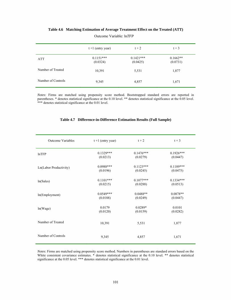
Table 4.6 Matching Estimation of Average Treatment Effect on the Treated (ATT)
Outcome Variable: lnTFP
t +1 (entry year) t + 2 t + 3
ATT 0.1151*** (0.0324)
0.1421*** (0.0425)
0.1662** (0.0731)
Number of Treated 10,391 5,531 1,877
Number of Controls 9,345 4,857 1,671
Notes: Firms are matched using propensity score method. Bootstrapped standard errors are reported in parentheses. * denotes statistical significance at the 0.10 level. ** denotes statistical significance at the 0.05 level. *** denotes statistical significance at the 0.01 level.
Table 4.7 Difference-in-Difference Estimation Results (Full Sample)
Outcome Variables t +1 (entry year) t + 2 t + 3
lnTFP 0.1329*** (0.0213)
0.1476*** (0.0279)
0.1926*** (0.0447)
Ln(Labor Productivity) 0.0988*** (0.0196)
0.1123*** (0.0245)
0.1189*** (0.0475)
ln(Sales) 0.1101*** (0.0215)
0.1077*** (0.0288)
0.1334*** (0.0513)
ln(Employment) 0.0549*** (0.0188)
0.0488** (0.0249)
0.0878** (0.0447)
ln(Wage) 0.0179 (0.0120)
0.0289* (0.0159)
0.0101 (0.0282)
Number of Treated 10,391 5,531 1,877
Number of Controls 9,345 4,857 1,671
Notes: Firms are matched using propensity score method. Numbers in parentheses are standard errors based on the White consistent covariance estimates. * denotes statistical significance at the 0.10 level. ** denotes statistical significance at the 0.05 level. *** denotes statistical significance at the 0.01 level.
101

Table 4.8 Difference-in-Difference Estimation Results (Subsamples)
Domestic Firms
__________________________________
Foreign Firms
__________________________________ Outcome Variables
t +1
(entry year) t + 2 t + 3
t +1
(entry year) t + 2 t + 3
lnTFP 0.1557*** (0.0244)
0.1606*** (0.0303)
0.2231*** (0.0528)
0.1002*** (0.0368)
0.1089** (0.0480)
0.1673** (0.0728)
ln(Labor
Productivity) 0.1179*** (0.0230)
0.1283*** (0.0298)
0.1324*** (0.0557)
0.0659* (0.0352)
0.0814* (0.0446)
0.0958 (0.0647)
ln(Sales) 0.1149*** (0.0257)
0.1101*** (0.0344)
0.1417*** (0.0632)
0.0943** (0.0375)
0.0959* (0.0491)
0.1109 (0.0822)
ln(Employment) 0.0510** (0.0226)
0.0494** (0.0241)
0.0901 (0.0532)
0.0475 (0.0324)
0.0444 (0.0424)
0.0869 (0.0720)
ln(Wage) 0.0187 (0.0139)
0.0296* (0.0169)
0.0105 (0.0316)
0.0216 (0.0224)
0.0075 (0.0289)
0.0042 (0.0458)
Number of Treated 6,893 3,619 1,130 3,442 1,928 753
Number of Controls 6,451 3,287 1,084 2,868 1,592 596
Notes: Firms are matched using propensity score method. Numbers in parentheses are standard errors based on the White consistent covariance estimates. * denotes statistical significance at the 0.10 level. ** denotes statistical significance at the 0.05 level. *** denotes statistical significance at the 0.01 level.
102

Table 4.9 Difference-in-Difference Estimation by Selected Industries
Code Industry
Number of
Treated
Number of
Controls
Average Treatment
Effect
13 Food Processing 321 243 0.1174 (0.0902)
14 Food Production 301 264 0.0762 (0.1045)
17 Textile 2314 1914 0.1432*** (0.0412)
18 Garments & Other Fiber Products 1273 965 0.1523*** (0.0575)
19 Leather, Fur, Feather and Related Products 454 386 -0.012 (0.1021)
20 Timber Processing, Bamboo, Cane &Palm 214 157 -0.0454 (0.1179)
24 Stationery, Educational & Sports Goods 324 261 0.1421 (0.1001)
26 Raw Chemical Materials & Chemical Products 612 544 0.1385** (0.0732)
30 Plastic Products 724 672 0.1082 (0.0841)
31 Nonmetal Mineral Products 512 484 0.0611 (0.0716)
34 Metal Products 701 662 0.1231* (0.0637)
35 General Machinery & Equipment Manufacturing 614 571 0.1121 (0.0823)
36 Special Machinery & Equipment Manufacturing 297 281 0.1735* (0.0936)
37 Transportation Equipment Manufacturing 363 315 0.1841* (0.0982)
40 Electric Equipment & Machinery 813 732 0.0904* (0.0521)
41 Electronic & Telecommunications 617 547 0.1390** (0.0671)
Notes: Firms are matched using propensity score method. Numbers in parentheses are standard errors based on the White consistent covariance estimates. * denotes statistical significance at the 0.10 level. ** denotes statistical significance at the 0.05 level. *** denotes statistical significance at the 0.01 level.
103

5. CONCLUSIONS
As shown by the studies of vertical specialization, FDI and exporting in this dissertation, market
forces and globalization forces changed China’s economy in a profound way. We find the
evidence that market reforms reduced transaction costs, increased vertical specialization, and
raising firms’ productivity. We also find the spillover effects of FDI and learning effects of
exporting.
Chapter 2 contributes to the literature by exploiting rich variation in regional market
development and vertical specialization in China’s manufacturing sector. Using instrumental
variable method, we find a statistically and quantitatively significant relationship between
vertical specialization and total factor productivity of firms. Our estimation results also indicate
that industry size, neighboring output and provincial marketization index are all determinants of
the vertical specialization. Thus, we find evidence that supports Smith’s extent-of-market theory,
Marshall’s input sharing theory and Coase’s transaction cost theory. By studying the quantitative
significance, we also find that transaction cost theory is more powerful in explaining vertical
specialization of firms. This finding implies that market-oriented reform that reduces transaction
costs is the major determinant of vertical specialization in China. We fail to find strong evidence
that supports Stigler’s theory of industry lifecycle.
In Chapter 3 we analyze productivity spillovers from foreign direct investment using
firm-level panel data from China manufacturing industries. We investigate whether there exist
productivity spillovers from FDI to domestic firms through horizontal, backward, forward and
104

local linkages. We apply the Levinsohn and Petrin (2003) method to the estimation of TFP,
which allows us to control for the potential endogeneity of input factors. The estimation results
from baseline specifications produce findings that support backward and local spillovers. As was
the case with previous studies on developing countries, little evidence of horizontal spillovers
can be found. As robustness checks, we distinguish spillovers from HMT investors versus OECD
investors, and export-oriented FDI versus domestic-market-oriented FDI. Moreover, we take into
account the absorptive capacity of domestic firms. The estimation results are consistent with our
main findings.
FDI is often regarded as an engine to economic development, an assumption that has led
many governments around the world to attract FDI by offering generous financial incentives.
Since we find positive backward and local spillovers, our study provides some support for such
policies.
Chapter 4 analyzes the relationship between firm productivity and export behavior in
China’s manufacturing firms. We find that firms that enter export markets show superior initial
performance compared to non-exporters; in other words, we discover evidence consistent with
self-selection theory. In order to determine the direction of causality between exporting and
productivity, we use propensity score matching technique to construct a counterfactual control
group. The matching method controls for the non-random selection of exporting firms in our
sample, and allows us to interpret our results as causal effects. Our findings suggest that
exporting leads to better performance of the firms. They become on average 13 percent more
productive after they start to export, which gives support to the learning-by-exporting hypothesis.
The results of this study are broadly consistent with the idea that increasing access to
export markets boosts productivity in developing countries. From an industrial policy
105

perspective, there is a good reason to promote foreign sales over domestic sales because firms
become better once they are active in export markets.
106

BIBLIOGRAPHY
Adelman, M. (1955) “Concepts of Statistical Measurement of Vertical Integration,” in G. Stigler
(ed.), Business Concentration and Price Policy, Princeton: Princeton University Press.
Ades, A., and E. Glaeser (1999) “Evidence on Growth, Increasing Returns, and the Extent of
Market,” Quarterly Journal of Economics, 114, pp. 1025-1045.
Aitken, B., and A. Harrison (1999) “Do Domestic Firms Benefit from Direct Foreign
Investment? Evidence from Venezuela,” American Economic Review, 89, pp. 605-618.
Aitken, B., A. Harrison, and R. Lipsey (1996) “Wages and Foreign Ownership: A Comparative
Study of Mexico, Venezuela, and the Unites States,” Journal of International Economics,
40, pp. 345-71.
Alvarez, R., and R. Lopez (2005) “Exporting and Performance: Evidence from Chilean Plants,”
forthcoming, Canadian Journal of Economics.
Andersen, E. (1998) “The Evolution of the Organisation of Industry,” DRUID working paper.
Aw, B., S. Chung, and M. Roberts (2000) “Productivity and Turnover in the Export Market:
Micro-level Evidence from the Republic of Korea and Taiwan (China),” World Bank
Economic Review, 14, pp. 65-90.
Bai, C., M. Du, Z. Tao, and S. Tong (2004) “Local Protection and Regional Specialization:
Evidence from China’s Industries,” Journal of International Economics, 63, pp. 397-417.
107

Baumgardner, J. (1988) “The Division of Labor, Local Market, and Worker Organization,”
Journal of Political Economy, 96, pp. 509-527.
Becker, G. (1981) “Altruism in the Family and Selfishness in the Market Place,” Economica, 48,
pp. 1-15.
Becker, G., and K. Murphy (1992) “The Division of Labor, Coordinating Costs, and
Knowledge,” Quarterly Journal Economics, 107, pp. 1137-1160.
Bellak, C. (2004) “How Domestic and Foreign Firms Differ and Why Does it Matter?” Journal
of Economic Surveys, 18, pp. 483-514.
Berliner, J. (1957) Factory and Manager in the USSR, Cambridge: Harvard University Press.
Bernard, A., J. Eaton, B. Jensen, and S. Kortum (2003) “Plants and Productivity in International
Trade,” American Economic Review, 93, pp. 1268-1290.
Bernard, A., and B. Jensen (1999) “Exceptional Exporter Performance: Cause, Effect, or Both?”
Journal of International Economics, 47, pp. 1-25.
Bernard, A., and J. Jensen (2004) “Why Some Firms Export,” Review of Economics and
Statistics, 86, pp. 561-568.
Bernard, A., and J. Wagner (1997) “Exports and Success in German Manufacturing,”
Weltwirtschaftliches Archiv, 133, pp. 134-157.
Blalock, G. (2002) “Technology from Foreign Direct Investment: Strategic Transfer though
Supplies Chains,” Dissertation at Haas School of Business, University of California,
Berkeley.
108

Blomstrom, M., and H. Persson (1983) “Foreign Investment and Spillover Efficiency in an
Underdeveloped Economy: Evidence from the Mexican Manufacturing Industry,” World
Development, 11, pp. 493-501.
Blundell, R., and M. Costa Dias (2000) “Evaluation Methods for Non-Experimental Data,”
Fiscal Studies, 2, pp. 427-468.
Borenstein, E., J. De Gregorio, and J-W Lee (1998) “How Does Foreign Direct Investment
Affect Economic Growth?” European Economics Review, 43, pp. 915-923.
Bound, J., D. Jaeger, and R. Baker (1995) “Problems with Instrumental Variables Estimation
When the Correlation between the Instruments and the Endogenous Explanatory
Variables is Weak,” Journal of the American Statistical Association, 90, pp. 443-450.
Castellani, D., and A. Zanfei (2002) “Technology Gaps, Absorptive Capacity and the Impact of
Inward Investments on Productivity of European Firms,” mimeo, University of Urbino,
Italy.
Caves, R. (1974) “Multinational Firms, Competition and Productivity in Host-Country Markets,”
Economica, 41, pp. 176-193.
Cheung, K.Y., and P. Lin (2003) “Spillover Effects of FDI on Innovation in China: Evidence
from the Provincial Data,” China Economic Review, 15, pp. 25-44.
Clerides, S., S. Lach, and J. Tybout (1998) “Is Learning by Exporting Important? Micro-dynamic
Evidence from Colombia Mexico, and Morocco,” Quarterly Journal of Economics, 113,
pp. 903-947.
Coase, R. (1937) “The Nature of the Firm,” Economica, 4, pp.386-405.
109

De Loecker, J. (2005) “Do Exporters Generate Higher Productivity? Evidence from Slovenia,”
working paper, Economics Department, K. U. Leuven.
Delgado, M., J. Farinas, and S. Ruano (2002) “Firm Productivity and Export Markets: a
Nonparametric Approach,” Journal of International Economics, 57, pp. 397- 422.
Dixit, A., and J. Stiglitz (1977) “Monopolistic Competition and Optimum Product Diversity,”
American Economic Review, 67, pp. 297-308.
Djankov, S., and B. Hoekman (2000) “Foreign Investment and Productivity Growth in Czech
Enterprises,” World Bank Economic Review, 14, pp. 49-64.
Edwards, S. (1998) “Openness, Productivity and Growth: What Do We Really Know?”
Economic Journal, 108, pp. 383-398.
Fine, C. (1998) Clockspeed, New York: Perseus Press.
Fujita, M., P. Krugman, and A. Venables (1999) The Spatial Economy, Cambridge: MIT Press.
Fan, G., X. Wang, and H. Zhu (2003) China’s Marketization Index by Province [Zhongguo
Fensheng Shichang Hua Zhishu], Beijing: Economic Science Press.
Garicano, L., and T. Hubbard (2003) “Specialization, Firms, and Markets: The Division of Labor
Within and Between Law Firms,” NBER Working Papers 9719.
Girma, S., D. Greenaway, and R. Kneller (2003) “Export Markets, Exit and Performance
Dynamics: A Causality Analysis of Matched Firms,” Economics Letters, 80, pp. 181-187.
Girma, S., and K. Wakelin (2002) “Are there Regional Spillovers from FDI in the UK?” in
Greenaway, David, Richard Upward, and Katharine Wakelin (ed.), Trade, Investment,
Migration and Labour Markets, Basingstoke: Macmillan.
110

Globerman, S. (1979) “Foreign Direct Investment and Spillover Efficiency Benefits in Canadian
Manufacturing Industries,” Canadian Journal of Economics, 12, pp. 42-56.
Gorg, H., and E. Strobl (2003) “Multinational Companies, Technology Spillovers and Plant
Survival,” Scandinavian Journal of Economics, 105, pp. 581-595.
Granick, D. (1960) The Red Executive: A Study of the Organization Man in Russian Industry,
Garden City: Doubleday.
Griliches, Z., and J. Hausman (1986) “Errors in Variables in Panel Data,” Journal of
Econometrics, 31, pp. 93-118.
Griliches, Z., and J. Mairesse (1998) “Production Function: The Search for Identification,” in S.
Stom (ed.), Econometrics and Economic Theory in the 20th Century: The Ragnar Frisch
Centennial Symposium, Cambridge University Press, U.K., pp. 169-203.
Grossman, S., and O. Hart (1986) “The Costs and Benefits of Ownership: A Theory of Vertical
and Lateral Integration,” Journal of Political Economy, 94, pp. 691-719.
Grossman, G., and E. Helpman (1989) “Product Development and International Trade,” Journal
of Political Economy, 97, pp. 1261-1283.
Grossman, G., and E. Helpman (2002) “Integration versus Outsourcing in Industry Equilibrium,”
Quarterly Journal of Economics, 117, pp. 85-120.
Haddad, M., and A. Harrison (1993) “Are There Positive Spillovers from Direct Foreign
Investment? Evidence from Panel Data for Morocco,” Journal of Development
Economics, 42, pp. 51-74.
111

Haskel, J., S. Pereira, and M. Slaughter (2002) “Does Inward Foreign Direct Investment Boost
the Productivity of Domestic Firms?” NBER Working Paper 8724.
He, X. (1990) Avenue towards Specialization of Production in Chinese Machinery Industry
[Zhongguo Jixie Gongye Zhuanye Hua De Daolu], Beijing: Machinery Industry
Publication House.
Heckman, J., H. Ichimura, and P. Todd (1997) “Matching as an Econometric Evaluation
Estimator,” Review of Economic Studies, 65, pp. 261-294.
Helpman, E., M. Melitz, and S. Yeaple (2004) “Export vs. FDI with Heterogeneous Firms,”
American Economic Review, 94, pp. 300-316.
Holmes, T. (1999) “Localization of Industry and Vertical Disintegration,” Review of Economics
and Statistics, 81, pp. 314-325.
Huang, Y. (2001) “The Role of Foreign-Invested Enterprises in the Chinese Economy: An
Institutional Foundation Approach,” in S. Chen and C. Wolf (eds.), China, the United
States and the Global Economy, Santa Monica, Rand Corporation.
Ippolito, R. (1977) “The Division of Labor in the Firm,” Economic Inquiry, 15, pp. 469-492.
Isgut, A. (2001) “What’s Different about Exporters? Evidence from Colombian Manufacturing,”
Journal of Development Studies, 37, pp. 57-82.
Jefferson, G., T. Rawski, L. Wang, and Y. Zheng (2000) “Ownership, Productivity Change, and
Financial Performance in Chinese Industry,” Journal of Comparative Economics, 28, pp.
786-813.
112

Javorcik, B. S. (2004) “Does Foreign Direct Investment Increase the Productivity of Domestic
Firms? In Search of Spillovers through Backward Linkages,” American Economic
Review, 94, pp. 605-627.
Ji, C., and W. Rong (1980) Actively Promote Industrial Specialization [Jiji Gaohao Gongye
Zhuanyehua Gongzuo], Beijing: China Social Sciences Press.
Jiang, X. (2002) China’s FDI Economy [Zhongguo De Waizi Jingji], Beijing: Renmin University
Press.
Kim, S. (1989) “Labor Specialization and the Extent of the Market,” Journal of Political
Economy, 97, pp. 692-705.
Keller, W., and S. Yeaple (2003): “Multinational Enterprises, International Trade, and
Productivity Growth: Firm-Level Evidence from the United States,” GEP Research Paper
03/03, University of Nottingham.
Kokko, A., R. Tansini, and M. Zejan (1996) “Local Technological Capability and Productivity
Spillovers from FDI in the Uruguayan Manufacturing Sector,” Journal of Development
Studies, 32, pp. 602-611.
Konings, J. (2001) “The Effects of Foreign Direct Investment on Domestic Firms: Evidence
from Firm Level Panel Data in Emerging Economies,” Economics of Transition, 9, pp.
619-633.
Kornai, J. (1980) Economics of Shortage, Amsterdam: North-Holland.
Kraay, A. (1999) “Exports and Economic Performance: Evidence from a Panel of Chinese
Enterprises,” Revue d’Economie Du Developpment, 1-2, pp. 183-207.
113

Krueger, A. (1995) “The Role of Trade in Growth and Development: Theory and Lessons from
Experience,” in R. Garnaut, E. Grilli, and J. Riedel (ed.), Sustaining Export-Oriented
Development: Ideas from East Asia, Cambridge: Cambridge University Press.
Krugman, P. (1979) “Increasing Returns, Monopolistic Competition, and International Trade,”
Journal of International Economics, 89, pp. 469-479.
Krugman, P. (1980) “Scale Economies, Product Differentiation, and the Pattern of Trade,”
American Economic Review, 70, pp. 950-959.
Langlois, R. (2000) “Capabilities and Vertical Disintegration in Process Technology: The Case
of Semiconductor Fabrication Equipment,” in N. Foss, and P. Robertson (ed.), Resources,
Technology, and Strategy: Explorations in the Resource-based Perspective, London:
Routledge Press.
Lardy, N. (2001) Integrating China into the Global Economy, Brookings Institution Press.
Lardy, N. (2005) “China’s Embrace of Globalization,” mimeo.
Leuven, E., and B. Sianesi (2003) “PSMATCH2: Stata Module to Perform Full Mahalanobis and
Propensity Score Matching, Common Support Graphing, and Covariate Imbalance
Testing,” http://ideas.repec.org/c/boc/bocode/ s432001.html.
Levinsohn, J., and A. Petrin (2003) “Estimating Production Functions Using Inputs to Control
for Unobservables,” Review of Economic Studies, 70, pp. 317-342.
Levy, D. (1984) “Testing Stigler’s Interpretation of `The Division of Labor is Limited by the
Extent of the Market,” Journal of Industrial Economics, 32, pp. 377-389.
Liu, Z., and P. Lin (2004) “Backward Linkages of Foreign Direct Investment: Evidence from
China,” mimeo, Lingnan University of Hong Kong.
114

Long, G. (2005) “China’s Policies on FDI: Review and Evaluation,” in T. Moran, E. Graham,
and M. Blomstrom (ed.), Does Foreign Direct Investment Promote Development?
Institution for International Economics, Washington DC.
Marshall, A. (1920) Principle of Economics, 8th edition, London: Macmillan.
Melitz, M. (2003) “The Impact of Trade on Intra-industry Reallocations and Aggregate Industry
Productivity,” Econometrica, 71, pp. 1695-1725.
Moulton, B. (1990) “An Illustration of a Pitfall in Estimating the Effects of Aggregate Variables
on Micro Units,” Review of Economics and Statistics, 72, pp. 724-726.
Murakami, N., D. Liu, and K. Otsuka (1996) “Market Reform, Division of Labor, and Increasing
Advantage of Small-Scale Enterprises: The Case of the Machine Tool Industry in China,”
Journal of Comparative Economics, 23, pp. 256-277.
National Statistical Bureau (1992) Explanations of the Main Statistical Indices in National
Economy [Guomin Jingji Zhuyao Tongji Zhibiao Jieshi], Beijing: China Statistical Press.
National Bureau of Statistics (1997) Organization and Implementation of Third National
Industrial Census [Di Sanci Quanguo Gonye Pucha De Zuzhi Yu Shishi], Beijing: China
Statistical Press.
Olley, G., and A. Pakes (1996) “The Dynamics of Productivity in the Telecommunication
Equipment Industry,” Econometrica, 64, pp. 1263-1297.
Pavcnik, N. (2002) “Trade Liberalization, Exit and Productivity Improvements: Evidence from
Chilean Plants,” Review of Economic Studies, 69, pp. 245-276.
115

Perry, M. (1989) “Vertical Integration: Determinants and Effects,” in Richard Schmalensee and
Robert Willig (ed.), Handbook of Industrial Organization, Netherlands: North-Holland.
Petrin, A., J. Levinsohn, and B. Poi (2004) “Production Function Estimation in Stata Using
Inputs to Control for Unobservables,” Stata Journal, pp. 113-123.
Plato, (380 BC) [1993] The Republic, translated by R. Waterfield, New York: Oxford University
Press.
Qian, P. (2003) “Industrial Clustering: A Strategy for China’s Economic Development,” [Chanye
Jiju: Zhongguo Jingji Fazhan Zhanlue], working Paper, China Development Research
Center.
Rawski, T. (1980) China’s Transition to Industrialism, Ann Arbor: University of Michigan
Press.
Rodrik, D. (1999) The New Global Economy and Developing Countries: Making Openness
Work, Policy Essay 24, Overseas Development Council, Johns Hopkins University Press,
Washington DC.
Rodrik, D., and F. Rodriguez (2000) “Trade Policy and Export Growth: A Skeptic’s Guide to the
Cross-Sectional Evidence,” in B. Bernanke and K. Rogoff (ed.), NBER Macroeconomic
Annual, Cambridge: MIT Press.
Romer, P. (1986) “Increasing Returns and Long-run Growth,” Journal of Political Economy, 94,
pp. 1002-1037.
Rosenbaum, P., and D. Rubin (1983) “Assessing Sensitivity to an Unobserved Binary Covariate
in an Observational Study with Binary Outcome,” Journal of the Royal Statistical
Society, Series B, 45, pp. 212-218.
116

Sgard, J. (2001) “Direct Foreign Investments and Productivity Growth in Hungarian Firms,
1992-1999,” William Davidson Institute Working Paper 425.
Sheng, H. (1994) Division of Labor and Transaction [Fengong Yu Jiaoyi], Shanghai: Shanghai
Sanlian Press and Shanghai People’s Publishing House.
Sjoholm, F. (1999) “Productivity Growth in Indonesia: The Role of Regional Characteristics and
Direct Foreign Investment,” Economic Development and Cultural Change, 47, pp. 559-
584.
Smarzynska, B., and M. Spatareanu (2002) “FDI Spillovers through Backward Linkages in
Romania: Some Determinants,” mimeo, World Bank.
Smith, A. (1776) [1976] The Wealth of Nations, reprinted, Chicago: University of Chicago Press.
Staiger, D., and J. Stock (1997) “Instrumental Variables Regression with Weak Instruments,”
Econometrica, 65, pp. 557-586.
Stock, J., and M. Yogo (2004) “Testing for Weak Instruments in Linear IV Regression,” working
paper, Department of Economics, Harvard University.
Stigler, G. (1951) “The Division of Labor is Limited by the Extent of the Market,” Journal of
Political Economy, 59, pp. 185-193.
Teece, D. (1977) “Technology Transfer by Multinational Firms: The Resource Cost of
Transferring Technological Know-How,” Economic Journal, 87, pp. 242-261.
Third National Industrial Census Office (1997) Collection of Materials of Third National
Industrial Census [Di Sanci Quanguo Gongye Pucha Ziliao Huibian], Comprehensive
and Industry Volume, Beijing: China Statistics Press.
117

Tong, S., and A. Hu (2003) “Do Domestic Firms Benefit from Foreign Direct Investment? Initial
Evidence from Chinese Manufacturing,” mimeo, University of Hong Kong.
Tucker, I., and R. Wilder (1977) “Trend in Vertical Integration in the U.S. Manufacturing
Sector,” Journal of Industrial Economics, 26, pp. 81-94.
UNCTAD (2003) World Investment Report 2003, UNCTAD: New York and Geneva.
Van Biesebroeck, J. (2005) “Exporting Raises Productivity in Sub-Saharan African
Manufacturing Firms,” Journal of International Economics, forthcoming.
Wagner, J. (2002) “The Causal Effect of Exports on Firm Size and Labor Productivity: First
Evidence from a Matching Approach,” Economics Letters, 77, pp. 287-292.
Williamson, O. (1975) Markets and Hierarchies: Analysis and Antitrust Implications, New
York: The Free Press.
Williamson, O. (1985) The Economic Institutions of Capitalism: Firms, Markets, Relational
Contracting, New York: The Free Press.
World Bank (1993) Foreign Direct Investment -- Benefits Beyond Insurance, Development Brief,
Washington DC.
World Bank (1998) World Development Report: Knowledge for Development, Oxford University
Press, New York.
Yang, X., and J. Borland (1991) “A Microeconomic Mechanism for Economic Growth,” Journal
of Political Economy, 99, pp. 460-482.
118

Wong, C., and R. Bird (2004) “China’s Fiscal System: A Work in Progress,” Conference on
China Economic Transition: Origins, Mechanisms and Consequences, November 5-7,
2004, Pittsburgh, PA.
Yi, K-M (2003) “Can Vertical Specialization Explain the Growth of World Trade?” Journal of
Political Economy, 111, pp. 52-102.
Young, A. (1928) “Increasing Returns and Economic Progress,” Economic Journal, 38, pp. 527-
542.
Young, A. (2000) “The Razor’s Edge: Distortions and Incremental Reform in the People’s
Public of China,” Quarterly Journal of Economics, 115, pp. 1091-1135.
Zhang, Y. (2005) “Local Government and Private Sector Development in China,” in S. Bao, S.
Lin, and C. Zhao (ed.), Chinese Economy after WTO Accession, UK: Ashgate Publishing
Limited.
119