Embed Size (px)
Citation preview

Essays on
Information and Heterogeneity
in Macroeconomics
by Piotr Denderski

ISBN: 978-90-3610-473-9
Cover design: Crasborn Graphic Designers bno, Valkenburg a.d. Geul
This book is no. 683 of the Tinbergen Institute Research Series, established through
cooperation between Rozenberg Publishers and the Tinbergen Institute. A list of books
which already appeared in the series can be found in the back.

VRIJE UNIVERSITEIT
ESSAYS ON INFORMATION AND HETEROGENEITY IN MACROECONOMICS
ACADEMISCH PROEFSCHRIFT
ter verkrijging van de graad Doctor aan
de Vrije Universiteit Amsterdam,
op gezag van de rector magnificus
prof.dr. V. Subramaniam,
in het openbaar te verdedigen
ten overstaan van de promotiecommissie
van de Faculteit der Economische Wetenschappen en Bedrijfskunde
op dinsdag 24 januari 2017 om 11.45 uur
in de aula van de universiteit,
De Boelelaan 1105
door
Piotr Rafał Denderski
geboren te Częstochowa, Polen

promotor: prof.dr. E. Bartelsman
copromotor: dr. B.A. Brügemann

Mojej rodzinie.
To my family.


Contents
Contents vii
1 Introduction 1
2 Public Data Quality and International Risk Sharing 9
2.1 Introduction . . . . . . . . . . . . . . . . . . . . . . . . . . . . . . . . . . 9
2.2 Public data quality and international risk sharing . . . . . . . . . . . . . 16
2.3 Environment . . . . . . . . . . . . . . . . . . . . . . . . . . . . . . . . . . 21
2.4 Analytical results . . . . . . . . . . . . . . . . . . . . . . . . . . . . . . . 25
2.5 Efficient allocations . . . . . . . . . . . . . . . . . . . . . . . . . . . . . . 32
2.6 Quantitative evaluation . . . . . . . . . . . . . . . . . . . . . . . . . . . . 36
2.7 Conclusions . . . . . . . . . . . . . . . . . . . . . . . . . . . . . . . . . . 48
2.A Proofs . . . . . . . . . . . . . . . . . . . . . . . . . . . . . . . . . . . . . 50
2.B Data and numerical solution . . . . . . . . . . . . . . . . . . . . . . . . . 62
3 Monetary Policy and Foreign-Owned Banks in Emerging Economies 65
3.1 Introduction . . . . . . . . . . . . . . . . . . . . . . . . . . . . . . . . . . 65
3.2 Data and Estimation Procedure . . . . . . . . . . . . . . . . . . . . . . . 69
3.3 Results . . . . . . . . . . . . . . . . . . . . . . . . . . . . . . . . . . . . . 73
3.4 Discussion and further tests . . . . . . . . . . . . . . . . . . . . . . . . . 80
3.5 Conclusions . . . . . . . . . . . . . . . . . . . . . . . . . . . . . . . . . . 81
3.A Data Description . . . . . . . . . . . . . . . . . . . . . . . . . . . . . . . 83
vii

4 A Model of Confounded Entrepreneurial Choice 87
4.1 Introduction . . . . . . . . . . . . . . . . . . . . . . . . . . . . . . . . . . 87
4.2 Empirical Facts . . . . . . . . . . . . . . . . . . . . . . . . . . . . . . . . 95
4.3 Basic Features of the Environment . . . . . . . . . . . . . . . . . . . . . 100
4.4 Learning . . . . . . . . . . . . . . . . . . . . . . . . . . . . . . . . . . . . 104
4.5 Illustration of the working of the model . . . . . . . . . . . . . . . . . . . 109
4.6 Quantitative Analysis . . . . . . . . . . . . . . . . . . . . . . . . . . . . . 116
4.7 Conclusions . . . . . . . . . . . . . . . . . . . . . . . . . . . . . . . . . . 123
4.A Plots and Tables . . . . . . . . . . . . . . . . . . . . . . . . . . . . . . . 124
4.B Proofs . . . . . . . . . . . . . . . . . . . . . . . . . . . . . . . . . . . . . 129
4.C Numerical algorithm . . . . . . . . . . . . . . . . . . . . . . . . . . . . . 135
5 Efficient insurance in market theory of payroll and self-employment 137
5.1 Introduction . . . . . . . . . . . . . . . . . . . . . . . . . . . . . . . . . . 137
5.2 Model environment . . . . . . . . . . . . . . . . . . . . . . . . . . . . . . 144
5.3 Equilibrium definition . . . . . . . . . . . . . . . . . . . . . . . . . . . . 147
5.4 Existence and efficiency of equilibrium . . . . . . . . . . . . . . . . . . . 152
5.5 Efficient insurance policy . . . . . . . . . . . . . . . . . . . . . . . . . . . 158
5.6 A dynamic model . . . . . . . . . . . . . . . . . . . . . . . . . . . . . . . 160
5.7 Conclusions . . . . . . . . . . . . . . . . . . . . . . . . . . . . . . . . . . 163
5.A Proofs for the static model . . . . . . . . . . . . . . . . . . . . . . . . . . 164
5.B Proofs for the dynamic model . . . . . . . . . . . . . . . . . . . . . . . . 174
Summary 179
Bibliography 183
Acknowledgements 193

Chapter 1
Introduction
Modern economics recognizes that frictions and differences between agents are key to
understanding the evolution of macroeconomic aggregates. However, it is the specific
research topic that determines the relevance of various aspects of heterogeneity and fric-
tions. This thesis is focused on two such topics. First, understanding the consequences
of international financial integration. Second, understanding how people choose in their
careers between payroll and self-employment.
At first sight these two are rather disconnected. Choice of those topics came from my
personal experience and background to which I relate shortly in the following sections.
However, there is a more subtle link that I only became aware of later in my studies.
The improvements in information technology that made countries more interconnected
also made it easier to dissect production chains and outsource some activities abroad
thus forcing people in developed economies to rely more on non-standard working ar-
rangements. On the other hand, they offered new ways of marketing one’s labor in the
market. Thus, these two research topics share, to a certain extent, a common cause in
the real world.

2 Introduction
International financial integration
The first two chapters of this dissertation are concerned with a process of integration
of financial markets that took off in the late 80s of the previous century. This was
prompted by technological advancement which made the information, people and goods
travel faster and more efficiently, by political integration, harmonization of regulations
etc. A starting observation about this process is that some countries, like emerging
economies in Latin America, South-East Asia or transition economies in Central and
Eastern Europe, including Poland, my home country, entered this process with inferior
production technologies and underdeveloped or absent local financial markets. Hence,
integration of financial markets had to involve vertical integration and take overs. Thus,
one of the chapters in my dissertation looks into the consequences of heterogeneous
ownership of banks (foreign, private, state owned) for the conduct of monetary policy
in Central and Eastern Europe.
Thirty years later we know (Obstfeld, 1995; Baxter, 2011; Kose et al., 2009; Bai and
Zhang, 2012) that the benefits of integration are distributed asymmetrically. In partic-
ular, international financial markets don’t provide much of insurance against country
specific idiosyncratic shocks to GDP to some countries while others do significantly bet-
ter. The literature (Chinn and Ito, 2006) has focused mostly on the role of economic
development and institutions. With my coauthor we take a different route and focus on
transparency and quality of publicly available information in explaining heterogeneity
in cross-country insurance against idiosyncratic GDP fluctuations.
In the first chapter of my dissertation, which is based on Denderski and Stoltenberg
(2016) we investigate the role of public data quality in international risk sharing. Based
on the Penn World Tables, we document a U-shaped relationship, implying that risk
sharing initially worsens and eventually ameliorates when data quality improves.
The U-shaped relationship between the quality of public information and risk shar-
ing is hard to explain in standard risk sharing models. In complete market models,

Introduction 3
better information has a monotone negative Hirshleifer (1971) effect: releasing better
information on idiosyncratic country risk realizations before trading harms social welfare
by limiting risk-sharing opportunities in international financial markets. In a standard
incomplete markets model on the other hand, countries can only self insure using a
non-state contingent bond. Here, better information helps countries to more accurately
make their decisions on borrowing and lending, leading to a monotone positive Blackwell
(1953) effect of information on risk sharing.
We develop a model that yields a prediction consistent with the data. In our model,
better public information has two opposite effects. First, it has a detrimental effect on
risk sharing by limiting risk-sharing possibilities as emphasized by Hirshleifer (1971).
Second, it mitigates the adverse selection problem resulting from private information
which improves risk sharing. The more severe is the private information friction in a
country, the more likely is that better public information improves risk sharing. As our
novel theoretical contribution, we provide a complete analytical characterization how
public and and non-contractible private information on future shocks affect risk sharing
in efficient insurance contracts.
In the second chapter of my dissertation, based on Denderski and Paczos (2016), we
provide new evidence on the bank lending channel of monetary policy using bank-level
panel data from Central and Eastern Europe economies. We examine loan granting
behavior of 440 banks in the period between 1998 and 2012.
The bank lending channel theory, analysed by Bernanke and Blinder (1992) on ag-
gregate data and Kashyap and Stein (2000) on bank-level data assumes that, at the
bank-level, deposits and other sources of financing are imperfect substitutes. Therefore,
when a central bank raises interest rates, the supply of credit at the bank level goes
down.
We find that foreign owned banks banks adjust their loans to changes in host coun-
try’s monetary policy. We test the conventional view behind the heterogeneity in bank
lending channel in foreign banks, the internal market hypothesis. This hypothesis im-

4 Introduction
plies that foreign owned banks trade with their parent bank and its other subsidiaries
which renders them less reliant on local cost of money.
We find that the data don’t uniformly support the claim that foreign banks are less
dependent on the cost of money in a host country because they may have access to funds
from parent banks. As an alternative we propose a market segmentation hypothesis. For-
eign banks may have a competitive advantage (better screening technology, inheritance
of customer relationship from parent bank country) so that their loan portfolio adjusts
less to changes in monetary policy instrument. Thus, increase in foreign penetration of
the banking sector does not necessarily render monetary policy less effective.
Next, we investigate the anatomy of the bank lending channel. We find that when
one focuses on all but ownership dimensions of bank level heterogeneity, the bank lend-
ing channel operates mostly through bank size. By incorporating type of ownership
heterogeneity we find that when the bank lending channel is confirmed in the data, it
is the foreign banks higher profitability that allows them to mute their response to the
monetary policy indicator.
We highlight two possible rationales. First, a foreign bank may inherit credit rela-
tionships with firms that are clients of its parent bank. When there is selection into
foreign expansion, then foreign-owned banks lend to more productive companies. Such
credit is less sensitive to changes of host country’s monetary policy because of implicit
costs embedded in adjusting terms of contracts. Second, if foreign-owned banks have
better know-how (e.g. screening technology or marketing) then they grant credit to more
reliable customers which can still service their liabilities under higher interest rates.
Type of employment choice
The other two chapters of this dissertation are on the drivers of type of employment
choice. My inspiration for pursuing this topic was my work as a free-lancer during my
studies in Warsaw. I then realised that self-employment involves operating in a more
complex environment than working as an employee, engaging a broader set of skills. It

Introduction 5
also seemed likely to me that more able people would, in general, do better in both types
of employment. Thus, finding out about one’s suitability to work in self-employment
seems to be a harder task but there is some cross-learning going on. Exactly this idea is
reflected in my job market paper which developes a model of correlated learning about
one’s abilities in the two types of employment. Because both types of employment
make use of heterogeneous individual abilities but self-employment requires supplying a
broader set of skills, identifying comparative advantage of a worker in self-employment
can be subject to confounding.
Finally, in the last chapter of the dissertation the role of different exposure to risk
in the two types of employment is investigated. Self-employed are the sole claimants of
the fruit of their labor but face risk of not selling their products/services on their own.
Searching for a job at a firm entails the risk of unemployment but offers a shield against
the risk in the goods market.
In the third chapter, based on Denderski (2016), I ask whether young people should
be encouraged to become entrepreneurs. The theory of occupational choice of Miller
(1984) prescribes experimenting with more uncertain jobs at the early stage of one’s
career for the sake of fast identification of one’s comparative advantages. According to
the theory, there is value in learning even in the case of entrepreneurial failure. However,
certain empirical findings put entrepreneurial learning in question.
First, entrepreneurs keep on running under-performing businesses, not switching
to payroll jobs even with long business tenure (Hamilton, 2000; Hurst and Pugsley,
2011). Thus, entrepreneurs are believed to be consistently over-optimistic to rationalise
frequent entry in face of low business survival rates (de Meza and Southey, 1996). I
argue it is the more complex “jack of all trades” nature of entrepreneurship that is
behind these facts. In my model, income of employees depends only on their ability
while entrepreneurial income depends jointly on the ability and the business acumen.
Both the factors are unknown and agents learn about them through noisy production.
Entrepreneurial income only provides one signal on two unobservables. Entrepreneurs

6 Introduction
who overestimate their acumen assign a fraction of disappointing performance to their
ability which leads to a “lock-in” effect in entrepreneurship. Early quits and switching
between the two types of employment, which produce high entry and exit rates, are
required to identify one’s business acumen. Reducing individual uncertainty on ability
improves productivity and selection into entrepreneurship.
The models of Roy (1951), Lucas (1978) and Jovanovic (1994) postulate that income
in one activity (entrepreneurship versus payroll employment) is a one to one function of
an ability dedicated solely to this particular activity. A notable exception is the “jack
of all trades” theory by (Lazear, 2004, 2005). According to this paper entrepreneurs are
generalists that have to do well in many different tasks, in contrast to specialists that
make great narrowly-focused employees. My paper can thus be viewed as a dynamic
learning version of Lazear (2004).
In the last chapter, based on Denderski and Sniekers (2016) we propose a theory of
self-employment which, contrary to earlier studies, does not rely on ex-ante heterogeneity
across agents. Households face a choice between self-employment and searching for a
job at a firm. Both labor and product markets have search frictions. In the mixed
equilibrium, households trade the risk of not meeting a customer when self-employed
against the risk of unemployment and the rent extraction in a guaranteed wage contract.
There is a variety of theories explaining self-selection into self-employment. A large
fraction of this literature puts individual characteristics and heterogeneity as a reason for
self-employment. We list a limited selection of those papers, whereas Parker (2004) offers
an extensive survey. Lucas (1978), Jovanovic (1982) and Poschke (2013) assume that
being an entrepreneur/self-employed requires a separate skill, potentially different than
a skill needed to be an employee. Kihlstrom and Laffont (1979) postulate differences in
risk aversion that lead to undertaking entrepreneurial activities. Lindquist et al. (2015)
document the importance of family background. We complement this literature, because
in our model self-employment is an equilibrium outcome that does not require any ex
ante individual heterogeneity.

Introduction 7
To the best of our knowledge, this chapter provides the first model of self-employment
with frictions in the goods market. Existing papers study the macroeconomic con-
sequences of goods market frictions (See e.g. Petrosky-Nadeau and Wasmer (2015);
Kaplan and Menzio (2013)), or characteristics of firms that operate in a frictional goods
market.
Under risk aversion of prospective workers, the equilibrium is inefficient under risk-
aversion due to excessive vacancy creation and self-insurance by self-employed, who
attract too many customers by low prices. Type of employment dependent differenti-
ated taxes and unemployment insurance benefits can restore efficiency under a balanced
budget.


Chapter 2
Public Data Quality and International Risk
Sharing
2.1. Introduction
International risk sharing has important consequences for social welfare. When coun-
tries’ engagement in international risk sharing is absent or not efficient, households in
those countries suffer from undesirable fluctuations in their consumption. The theoreti-
cal literature has emphasized the importance of public and private information for risk
sharing in general.1 However, relatively little is known about how the quality of infor-
mation affects international risk sharing in reality. Based on the Penn World Tables,
we document and explain a novel fact: there are significant differences in international
risk sharing across countries depending on countries’ public information quality on real
GDP.
After controlling for observable differences between countries such as the stage of eco-
nomic development and measures of financial openness, we find a U-shaped relationship
between public data quality and a country’s degree of international risk sharing. The
differences in risk sharing resulting from public data quality are not negligible. Coun-
1Exemplary papers are Schlee (2001); Atkeson and Lucas (1992) or the classical paper by Hirshleifer(1971)

10 International Risk Sharing
tries with low quality of information achieve a degree of risk sharing (0.31) that is more
than two times higher than the degree of risk sharing in countries with medium quality
(0.14) but lower than risk sharing in countries with high data quality (0.35).2 However,
the Global Open Data Index project (http://index.okfn.org) documents that countries
do not necessarily provide all relevant information they possess. Thus, we argue that
the U-shaped relationship can be rationalized as a result of an interaction between the
country’s quality of public information and its degree of transparency.
The U-shaped relationship between the quality of public information and risk shar-
ing is hard to explain in standard risk sharing models. In complete market models,
better information has a monotone negative Hirshleifer (1971) effect: releasing better
information on idiosyncratic country risk realizations before trading harms social welfare
by limiting risk-sharing opportunities in international financial markets. In a standard
incomplete markets model on the other hand, countries can only self insure using a
non-state contingent bond. Here, better information helps countries to more accurately
make their decisions on borrowing and lending, leading to a monotone positive Blackwell
(1953) effect of information on risk sharing.
In our model, representative households or governments of small countries insure
against country-specific shocks to real GDP by engaging in risk sharing with a complete
set of contracts on international financial markets. There are, however, endogenous
limits to risk sharing because contract enforceability is limited. In any period follow-
ing the realization of idiosyncratic risk, countries have the option to walk away from
the arrangement with the consequence of exclusion from international risk sharing as in
Grossman and Huyck (1988) and Bulow and Rogoff (1989). Limited contract enforce-
ment is motivated by the lack of a supranational authority to guarantee compliance with
the terms agreed in international borrowing and lending arrangements. In equilibrium,
consumption allocations across countries follow from optimal state-contingent insurance
contracts. As in Hirshleifer (1971), the model features complete financial markets but
2In Section 2.2, we provide the details on the country panel and on the estimation strategy.

Introduction 11
the model does not necessarily yield full insurance due to imperfect contract enforce-
ment. On the contrary, when contract enforcement matters, country-specific shocks can
only be partially insured.
Each country receives in every period two orthogonal signals on their future id-
iosyncratic income realization, private and public signals. The public signals capture
information on a country’s future GDP that is publicly available to other countries, for
example the real GDP growth forecast provided in the IMF World Economic Outlook
(WEO). Private signals are exclusively observed by a particular country. Thus, private
signals capture how transparent a country is in granting access to national statistics.
A high precision of private signals indicates secrecy, i.e., useful information exists but
that information is not publicly shared. This may happen for example because of in-
stitutional lags or legal boundaries to revelation or processing of information and data
provided. Thus, we assume that private information is not contractible and becomes
a friction which can reduce risk sharing possibilities in equilibrium. The more precise
are private signals, the more severe is the drop in risk sharing caused by the private
information friction.
As our novel theoretical contribution, we provide a complete analytical characteri-
zation how public and and non-contractible private information on future shocks affect
risk sharing in efficient insurance contracts.
In particular, we formally show that better public information can be beneficial
for risk sharing when private information is sufficiently precise. To the best of our
knowledge, our paper is the first in showing that releasing better public information can
improve risk sharing in an environment with a full set of state-contingent securities. The
positive effect of public information on risk sharing is intriguing but can be understood as
a trade off between costs and benefits from releasing more precise public signals. In our
model, better public information has two opposite effects. First, more informative public
signals increase the riskiness of the consumption allocation that can be supported in self-
enforceable arrangements. Second, however, more informative public signals mitigate
12 International Risk Sharing
the private information friction and thereby lead to better risk sharing. When private
information is sufficiently precise, risk sharing improves with better public information
and countries prefer informative public signals.
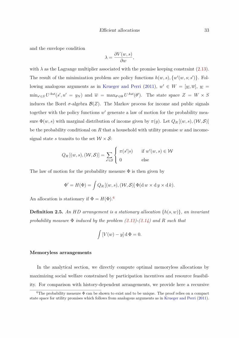
Further, we show that the importance of the private information friction not only
influences the amount of risk sharing in equilibrium but also to what extent past events
can enter the terms of the optimal insurance contract. In general, the optimal insur-
ance contract is contingent on the history of income shocks a country has experienced.
However, the more important is non-contractible private information, the shorter is the
history of income shocks that can be contracted upon in the efficient insurance contract.
As one extreme, the optimal insurance can not be contingent on any shock history but
only on current income shocks. Thus, the more private information a country has about
its future real GDP, the more difficult it becomes for the country to negotiate long-term
debt arrangements.
Based on the Penn World Tables, we construct a panel that comprises 75 countries
from 1991 to 2004. After controlling for observable differences between countries such
as the level of development and financial openness, we employ the data quality grades
provided in the Penn World Tables to bin countries’ risk sharing with respect to the
quality of public information. The data-quality grades rank from the highest data-
quality A to the lowest quality D. Thereby, a low data quality grade can result for
example because information on real GDP is not reported and thus incomplete or when
real GDP figures are sensitive with respect to the particular method used in aggregation.
To quantify public data quality, we compute mean-squared forecast errors based on the
IMF WEO and scale the error by the country’s volatility of income growth. The degree of
risk sharing is measured following the tradition of Obstfeld (1995) by regressing country-
specific fluctuations in consumption growth on country-specific fluctuations of income
growth. With this data and methodology, we estimate a U-shaped relationship between
the quality of public information and the degree of international risk sharing.
To take the model to the data, we calibrate the volatility of country-specific income

Introduction 13
shocks to match the corresponding estimated volatility of real GDP in the Penn World
Tables. For the quality of public information, we vary the precision of public signals until
the implied mean forecast squared-error for GDP growth in the model yields the error as
estimated from the WEO data. The unobservable precision of private signals is identified
using the model such that the cross-country consumption distribution in equilibrium
mimics the degree of risk sharing estimated in the country panel. Ex-ante, countries
are heterogenous with respect to the quality of public information and the degree of
transparency captured by the precision of private signals. Ex-post, countries differ with
respect to their success in smoothing their consumption in response to country-specific
shocks.
Quantitatively, we find that the model can capture the U-shaped relationship between
risk sharing and the quality of information. Private information plays a key role in
generating this relationship. In particular, the model suggests that countries with a
medium public data quality such as Portugal, South Korea and Spain are countries in
which the private information friction plays an important role, resulting in the relatively
low degrees of international risk sharing observed in the data. This interpretation is
consistent with findings of the Global Open Data Index project. While for all of the
countries with a medium public data quality in our sample data on national statistics
exist, none of the countries provided the data openly licensed until at least 2013, i.e.,
legally the data could not be freely reused and distributed to forecast real GDP growth.
Since our model captures the new stylized fact from the data, we can ask how better
public data quality affects risk sharing and welfare. We consider two scenarios for the
release of better public information. In the first scenario, data quality improves because
the IMF improves her real GDP growth forecast for a group of countries. The second
scenario captures the possibility that countries change their disclosure policies toward
transparency and release their private information on the country’s future GDP growth
to the worldwide public.
We find that in countries with an important private information friction, better public

14 International Risk Sharing
data quality improves risk sharing in both scenarios. Quantitatively, the improvements
in risk sharing resulting from changes in disclosure policies of countries towards trans-
parency are ten times more important than the improvements achieved by better IMF
forecasts. In both scenarios, better data quality in a particular group of countries can
trigger positive spillover effects to risk sharing and welfare in other countries.
Related Literature The main novel contribution of this paper is to document the
U-shaped relationship between public data quality and international risk sharing and to
develop a model to explain it.
The most closely related paper is Broer, Klein, and Kapicka (2015) who analyze the
effect of unobservable income shocks on consumption risk sharing of U.S. households
when contract enforcement is limited. As in Atkeson and Lucas (1992, 1995), agents
can be induced to report their income truthfully and private information reports become
contractible. The main difference is that we consider public and non-contractible private
signals on future income shocks, current income shocks are publicly observable. Our
focus is on documenting and rationalizing the role of public data quality in international
risk sharing.
With this paper, we build a bridge between the theoretical literature on the social
value of information (Morris and Shin, 2002; Schlee, 2001; Hirshleifer, 1971) and the
quantitative literature on sovereign risk (Arellano, 2008; Bai and Zhang, 2012).
Hirshleifer (1971) is among the first to point out that perfect information makes
risk-averse agents ex-ante worse off if such information leads to evaporation of risks
that otherwise could have been shared in a competitive equilibrium with full insurance.
Schlee (2001) provides general conditions under which better public information about
idiosyncratic risk is undesirable in a competitive equilibrium. There are two main dif-
ferences to these papers in our work. First, we consider optimal insurance contracts
with limited enforcement that hinder agents from full insurance. Second, we allow for
two sources of information, private and public. Notably, our main theoretical result on

Introduction 15
the positive effect of public information only applies in the empirically realistic case of
partial insurance and when private information is important.
In a global games framework, Morris and Shin (2002) show that when the coordi-
nation of agents is driven by strategic complementarities in their actions, better public
information on aggregate shocks may be undesirable in the presence of private informa-
tion on these shocks. The main difference to Morris and Shin (2002) is that we analyze
the social value of private and public information on idiosyncratic shocks in international
risk sharing.
Arellano (2008) and Bai and Zhang (2012) consider economies in which small coun-
tries engage in international risk sharing using non-state contingent bonds. Arellano
(2008) focuses on the interaction of sovereign default with output, consumption and
interest rates over the business cycle. Bai and Zhang (2012) ask whether financial lib-
eralization helped to improve on the insurance of idiosyncratic country risk. None of
these papers focuses on the relationship between data quality and risk sharing. Further,
with non-state contingent bonds, improving public and private data quality would both
have an indistinguishable and monotone positive effect on risk sharing. To capture the
documented non-monotone relationship between public data quality and risk sharing,
we develop a model with public and private information and a complete set of securities
with limited enforcement of contracts.
The remainder of the paper is organized as follows. In the next section, we document
cross-country differences in risk sharing with respect to the quality of public information.
Afterwards, we present the theoretical model and show analytically that it has the
potential to explain the risk-sharing differences observed in the data. In Section 2.6,
we take the model to the data and provide normative implications. The last section
concludes.

16 International Risk Sharing
2.2. Public data quality and international risk sharing
Using a large panel of countries, we ask how better public information affects in-
ternational risk sharing in the data. As our key result, we find that the relationship
between public information and risk sharing in the cross section follows a U-shape. For
low quality of public information, improvements in public information deteriorate risk
sharing, further improving data quality however ameliorates the degree of international
risk sharing. This fact is robust to controlling for the level of economic development and
financial integration, two measures that are widely recognized to be important drivers
of international risk sharing.
To empirically assess how risk sharing varies across countries that differ with respect
to public data quality, we employ data on real consumption and real GDP per capita from
the Penn World Tables, version 8.1. We use two different measures to assess the quality
of public information on real GDP. The first measure is discrete and is given by the data
quality grade provided in the Penn World Tables. The data-quality grades rank from the
highest data-quality A to the lowest quality D. Thereby, a low data quality grade can
result for example because information on real GDP is not reported and thus incomplete
or when real GDP figures are sensitive with respect to the particular method used in
aggregation. As a second measure and based on data from the IMF World Economic
Outlook, we compute mean squared forecast errors for real GDP growth for all countries
in our sample and scale them by the variance of GDP growth. We generate measures of
risk sharing by regressing the idiosyncratic component of changes in consumption per
capita in country i on the idiosyncratic component of changes in GDP per capita.
To facilitate comparisons with related studies, we build our sample starting with the
data of Kose, Prasad, and Terrones (2009), a study that utilised Penn World Tables data
to investigate the evolution of the risk sharing measures in time. However, Kose et al.
(2009)’s sample contains only one D-quality grade country (Togo). Thus, we expand the
sample by adding D-quality grade countries with population no smaller than 1 million

Public data quality and international risk sharing 17
inhabitants. Eventually, our data set comprises observations on 75 countries for the
years 1991-2004. In Appendix 3.A, we provide further details about the final sample.
Results As a first step, for each country in our data we compute the mean squared
error of one year ahead IMF GDP growth rate forecasts relative to actual realized real
GDP growth over the sample period. This measure closely corresponds to the treatment
of information in our model presented in the next section, however, because this measure
is scale dependent, we normalize it by country’s realized GDP growth rate variances.
In Table 2.1, we report the averages of normalized mean squared errors for each of the
public data quality country groups. The resulting monotone pattern confirms the data
quality grade assignment from the Penn World Tables.
We proceed with documenting the relationship between data quality grade and in-
ternational risk sharing. Following Obstfeld (1995), for each country i in our sample we
separately run a baseline risk sharing regression:
∆ ln (cit) − ∆ ln (Ct) = β0i + β1i [∆ ln (yit) − ∆ ln (Yt)] + εit, (2.1)
where ∆cit/yit stands for country’s i log-difference of consumption/GDP per capita
in year t. Capital letter variables are logs of sample aggregates intended to capture
uninsurable aggregate risk. The standard measure of risk sharing is β∆y,i ≡ 1 − β1i
which attains 0 (no insurance) if changes in country’s i consumption growth react one-
to-one to changes in country’s i GDP growth rate and 1 if consumption growth does not
react to changes in GDP growth at all (full insurance).
A representative risk averse household would ideally fully smooth its consumption,
thus insuring itself against the idiosyncratic fluctuations in GDP. Feasibility of such an
allocation crucially relies on the possibilities of trading in international asset markets
with representative households of other countries. Hence, in this sense, this regression
measures the degree of risk sharing against country-specific risk, one that could not be
insured against within the country itself.

18 International Risk Sharing
For each data quality grade group, we report an average β∆y,i as an unconditional
risk sharing coefficient in the second row of Table 2.1. Group A countries attain the
highest level of risk sharing, nearly three times as high as countries in group B and
twice as large as for C-countries. For D countries, we face data limitations: except for
one country, there is no consumption data available in the Penn World Tables. For this
reason, we exclude these countries from the risk-sharing regressions. The IMF data on
GDP growth rate forecasts and realizations includes D countries and we employ these
countries as a reference point for calibrating public information precision.
Next, we run a panel risk sharing regression adding interactions with country fixed
effect:
∆ ln (cit) − ∆ ln (Ct) = β0 + (β1 + βi) [∆ ln (yit) − ∆ ln (Yt)] + εit.
We report resulting group averages of risk sharing coefficients βF E∆y,i = 1 − β1 − βi in
the third row of Table 2.1. The U-shaped pattern prevails, however, the advantage of
A-countries over the other two groups of countries decreases.
Following the practice in the international risk sharing literature, we control for the
effect of the level of development and the degree of financial integration on risk sharing.
In the second step, we regress the country specific risk sharing coefficients β∆y,i on
combinations of controls that include the log of the average GDP per capita ln (yi) and
a measure of within-period average financial integration FinInti
β∆y,i = γ0 + γGDP ln (yi) + γF IFinInti + ζi. (2.2)
Subsequently, we control for three measures of financial integration. The first one
is the Chinn-Ito index (Chinn and Ito, 2006) which is derived from a set of underlying
measures of financial openness of a country. The other two measures are the ratio of
total assets and liabilities to GDP taken from the External Wealth of Nations Database.
Unlike the Chinn-Ito index which is a continuous de jure measure of financial integration,
the other two measures are de facto measures.

Public data quality and international risk sharing 19
Table 2.1
Data quality, forecast accuracy and risk sharingMSFEj is the annual mean-squared forecast error in country group j ∈ {A, B, C} normalizedby the variance of GDP growth. IMF World Economic Outlook Forecast for GDP growth inyear t is given by the Fall forecast in t − 1, the GDP growth realization is given by the valuereported in Fall t+1. Financial integration measure is the Chinn-Ito index. Data: Penn WorldTables, IMF World Economic Outlook, 1991–2004.
Data Quality GradeA B C D
MSEj , normalized 1.04 1.15 1.26 1.49
Risk sharing, β∆y,j , uncond. 0.46 0.16 0.22 −Risk sharing, β∆y,j , uncond., country FE 0.40 0.20 0.22 −Risk sharing, β∆y,j , cond. 0.35 0.14 0.31 −
In the last row of Table 2.1, we report conditional risk sharing coefficients for the
data-quality groups A, B and C3. This exercise demonstrates that the inferior risk
sharing of countries in groups B and C compared to the highest grade A countries
is partly driven by differences in level of economic development and their economies’
financial integration. For example, grade C countries tend to have lower average GDP
per capita levels than countries in A and B group. In fact, about 80 percent of the
difference in risk sharing between groups A and C can be attributed to the level of
economic development and financial integration; B countries’ decrease in risk sharing
from 0.16 to 0.14 is due to their relatively high level of GDP per capita and substantial
openness as compared to C countries.
The main message is that improvements in public data quality on country’s idiosyn-
cratic GDP risk, do not impact on risk sharing monotonically. Increasing data quality
from grade C to B worsens risk sharing but further improvements ameliorate risk shar-
ing.
The pattern that we report here survives the use of alternative specification of con-
trols in the first stage regression. Details of those tests are provided in Appendix 3.A.
The magnitude of the differences in risk sharing across countries depends only to a3Residuals ζi centered at β∆y,i, the sample average from regression with GDP as the sole control.

20 International Risk Sharing
small extent on the specification of controls (see Table 2.B.1). To address this issue, we
formally test the significance of differences between countries relative to the B group.
When regressing the conditional risk sharing coefficients on dummies that identify A and
C countries, we find that the low degree of risk sharing in B countries is statistically
significant (see Table 2.B.2).
Measurement Error Theoretically, the U-shaped pattern that we find in the data
could be driven by a measurement error in the explanatory variable that is potentially
the largest for C countries. It is well known that a classical measurement error in the
explanatory variable can introduce an attenuation bias, thus lowering the estimated
β1i coefficients in regression (2.1). Formally, if the true data ∆y∗it is measured with
noise, ∆yit = ∆y∗it + εm.err. and the true underlying first stage coefficient is β∗
1i then the
estimated value β1i in the limit reads:
β1i =σ2
∆ ln(y∗it)−∆ ln(Y ∗
t )σ2
∆ ln(y∗it)−∆ ln(Y ∗
t ) + σ2m.err.
β∗1i ≡ λβ∗
1i (2.3)
The attenuation factor λ depends solely on the variances of the measurement error and
the true data ∆y∗it. Getting rid of this error could bring the C-group risk sharing measure
below the one of the B-countries, breaking the U-shaped pattern as a result. It seems
unlikely, however, that the measurement error could be the sole driver of the U-shaped
pattern, for at last two reasons.
First, assuming measurement error independent of the second-stage regressors and
that risk sharing measures for A and B countries were estimated without attenuation
bias, we can use (2.3) to compute the magnitude of the measurement error variance
necessary to yield the conditional β∆,j identical for B and C-countries. Back of the
envelope calculations yield that the measurement error variance would have to be equal
to one-fourth of the true GDP change variance in C-countries. To put it differently,
one-fifth of the observed GDP changes in C-countries would have to be coming from
mis-measurement. Thus, a C-country growing on average by 4 percent on an annual
basis could accumulate to a level of GDP that is mis-measured by 10 percent after a

Environment 21
decade which is not plausible.
Second, C-group comprises the poorest and the least integrated countries in our
sample. Thus, in the second stage regression we would recover an even stronger positive
effect of average GDP and financial openness on the risk sharing measure β∆y,j. This
could decrease the average conditional β∆y,j of B-countries even more relative to the
average conditional β∆y,j of C-countries. Hence, it’s not clear that the direction of the
difference in conditional risk sharing measures could be explained by the measurement
error.
We conclude that although the measurement error can affect the numbers that we
report, it’s unlikely that it can break the U-shaped pattern between public data quality
and risk sharing. In the following sections, we present a theoretical model to rationalize
the U-shaped pattern observed in the data.
2.3. Environment
Preferences and endowments Consider a world economy that is populated by a
continuum of representative households or benevolent governments of small countries
indexed i and limited enforcement of contracts as in as in Kehoe and Levine (1993) and
Krueger and Perri (2011). The time is discrete and indexed by t from zero onward.
Households have identical preferences over consumption streams
U ({ct}∞t=0) = (1 − β) E0
∞∑t=0
βtu(ct), (2.4)
where the instantaneous utility function u : R+ → R is strictly increasing, strictly
concave and satisfies the Inada conditions.
The income stream of household i, {yit}∞
t=0, is governed by a stochastic process where
the set of possible realizations in each period is time invariant, ordered and finite: yit ∈
Y ≡ {y1, ..., yN} ⊆ R++, and yt denotes the history (y0, ...yt). Income realizations are
independent across households and evolve across time according to a first-order Markov
chain with constant transition probabilities π(y′|y). The Markov chain induces a unique

22 International Risk Sharing
invariant distribution of income π(y) such that average income is y = ∑y yπ(y). Current-
period income is publicly observable and the transition probabilities of the Markov chain
are public knowledge.
Information and utility allocation Each period t ≥ 0, household i receives a public
signal kit ∈ Y (observed by all representative households) and a private signal ni
t ∈ Y
(observed only by household i) that inform about her income realization in the next
period. Both signals have as many realizations as income states and are assumed to
follow exogenous independent first-order Markov processes. Further, both processes
exhibit the same transition probabilities as income, i.e., π(k′ = yj|k = yi) = π(y′ =
yj|y = yi). The precision of the public signal is denoted by the conditional probability
κ = π(y′ = yj|k = yj), while the precision of the private signal is given by ν = π(y′ =
yj|n = yj), κ, ν ∈ [1/N, 1]. Uninformative signals are characterized by precision 1/N
while perfectly informative signals exhibit precision of one. The pair (κ, ν) captures both
how good the public data quality is and how transparent a country is. A country with
high precision of public but low precision of private signals has a high public data quality
and is transparent; a country with low public signal but high private signal precision is
characterized by low public data quality and secrecy.
The publicly observable part of the state vector is st = (yt, kt), st ∈ S, where
S = Y ×Y . Let st = (yt, kt) denote the public history of the state (s0, ...st). The history
of the public and private state is denoted by θt = (st, nt), with θt ∈ Θ = S ×Y . The con-
ditional distribution of signals and income is a time-invariant Markov chain described by
transition matrices Pθ, Ps with the conditional probabilities π(θ′|θ) and π(s′|s).4 House-
holds differ with respect to their initial utility entitlements w0 and the initial state θ0.
For all θt, the utility allocation is h = {ht(w0, θt)}∞t=0 = {ht(w0, st)}∞
t=0 and the con-
sumption allocation c can be obtained as c = {C (ht(w0, st))}∞t=0, where C : R → R+
is the inverse of the instantaneous utility function u. Thus, the allocation is assumed
to be contingent solely on the public state, private information is not contractible and
4The computation of the conditional probabilities can be found in Appendix 2.A.

Environment 23
Figure 2.1
Timing of events
-t t + 1
?
Income
yit
?
Signals
kit, ni
t
?
Decision?
Exchange?
Consumption
cit
cannot be revealed for institutional reasons.
International risk sharing arrangements To protect their consumption from un-
desirable fluctuations, households can engage in insurance contracts that cover the com-
plete state space but have limited enforceability because households have the option to
default to autarky. As illustrated in Figure 5.2, each period after receiving the cur-
rent income and the two signals, households can decide to participate in international
risk-sharing contracts implementing the allocation c or to deviate into autarky forever
consuming only their income. Households have no incentive to default if the allocation
satisfies enforcement or participation constraints for each history θt and all periods t
(1 − β)u (C (ht)) + β∑θt+1
π(θt+1|θt)Ut+1({C (hτ )}∞
τ=t+1
)≥
(1 − β)u(yt) + β∑yt+1
π(yt+1|θt)Ut+1({yτ }∞
τ=t+1
)= UAut(θt), (2.5)
with ht = ht(w0, st), hτ = hτ (w0, sτ ), Uτ = (1 − β) Eτ∑∞
t=τ βt−τ u (ct) and UAut(θt) as
the value of the outside option (autarky). While private information is not-contractible,
it nevertheless influences the consumption allocation through countries’ incentives to
participate in international risk sharing or to deviate to autarky.
Optimal allocations Let Φ0 be a distribution over initial utility promises w0 and the
initial shocks s0. In the following definitions, we summarize the notions of constrained
feasible and efficient allocations.
Definition 2.1. An allocation h = {ht(w0, st)}∞t=0 is constrained feasible if

24 International Risk Sharing
(i) the allocation delivers the promised utility w0
w0 = (1 − β) Es0
[ ∞∑t=0
βtht(w0, st)]
= U(w0, s0, c); (2.6)
(ii) the allocation satisfies enforcement constraints (2.5) for each history θt in each
period t
(iii) and the allocation is resource feasible for for each history θt in each period t
∑θt
∫[C (ht) − yt] π(st|s0) d Φ0 ≤ 0. (2.7)
Atkeson and Lucas (1992, 1995) show by applying a duality argument that efficient
allocations can be computed either by directly maximizing households’ utility over the
distribution Φ0 or, alternatively, by minimizing resource costs to deliver the promises
made in Φ0.
Definition 2.2. An allocation {ht(w0, st)}∞t=0 is efficient if it is constrained feasible and
either
(i) maximizes households’ ex-ante utility over the distribution Φ0
E U(c) =∫
U(w0, s0, c) d Φ0
(ii) or, that there is no other constrained feasible allocation {ht(w0, st)}∞t=0 with respect
to Φ0 that requires fewer resources in at least one period t
∃t :∑θt
∫ [C(ht
)− C (ht)
]π(st|s0) d Φ0 < 0.
The second part of the definition is relevant with a continuum of agents and when
allocations depend on the state history. Using the first approach, there would be a
continuum of promise-keeping constraints (2.6) the planner would have to respect which
makes the approach to optimize directly over ex-ante utility impossible. The first ap-
proach can be applied however in the absence of promises as a state variable such that
allocations just depend on the current state but not on the history. We refer to such
allocations as memoryless allocations which are defined as follows.

Analytical results 25
Definition 2.3. An allocation {ht(w0, st)}∞t=0 is a memoryless allocation (denoted hML)
if:
∀st{ht(w0, st)
}∞
t=0= {ht(st)}∞
t=0 ≡ hML.
In the next section, we employ the simplified structure resulting from memoryless
allocations to derive analytical results on how the interplay of public and private infor-
mation affects risk sharing.
2.4. Analytical results
In this section, we show analytically that the model has the potential to capture
the U-shaped relationship between public data quality and risk sharing observed in the
data. In particular, we find that countries with more precise public signals can have lower
degrees of risk sharing if these countries are less transparent. As our main normative
result, we find that public data improvements by the IMF can improve or worsen risk
sharing depending how transparent a country is.
To analytically characterize the welfare effect of public information, we abstract in
this section from a number of features. First, we assume that the set of possible income
realizations consists of two states, a high income yh = y+δy and a low income yl = y−δy,
where δy > 0 is the standard deviation of income. Second, the states are equally likely
and the income realizations are independent across time and agents. Correspondingly,
signals are i.i.d. as well and can indicate either a high income (“good” or “high” signals)
or a low income (“bad” or “low” signals) in the future. By definition, a memoryless
allocation does not depend on past events but just on current realizations of the state.
A utility allocation in this simplified setting is hML = {u(cj
i
)}, with cj
i = C[h(y =
yj, k = yi)] and social welfare is
E U(c) = (1 − β)14
∞∑t=0
∑j∈{l,h}
∑i∈{l,h}
βtu(cj
i
). (2.8)

26 International Risk Sharing
Resource feasibility requires in each period t
14
∑j∈{l,h}
∑i∈{l,h}
cji = 1
2∑
j∈{l,h}yj. (2.9)
Further, constrained feasibility requires that allocations are consistent with rational in-
centives to participate. For example, the enforcement constraints of high-income house-
holds with high public and high private signals are
(1 − β)u(chh) +
β(1 − β)[κνV h
rs + (1 − κ)(1 − ν)V lrs
]κν + (1 − κ)(1 − ν)
+ β2Vrs ≥
(1 − β)u(yh) + β(1 − β) [κνu(yh) + (1 − κ)(1 − ν)u(yl)]κν + (1 − κ)(1 − ν)
+ β2Vout, (2.10)
while the constraints for high-income agents with low public and high private signals
read
(1 − β)u(chl ) +
β(1 − β)[(1 − κ)νV h
rs + κ(1 − ν)V lrs
](1 − κ)ν + κ(1 − ν)
+ β2Vrs ≥
(1 − β)u(yh) + β(1 − β) [(1 − κ)νu(yh) + κ(1 − ν)u(yl)](1 − κ)ν + κ(1 − ν)
+ β2Vout, (2.11)
with
V hrs = 1
2[u(ch
h) + u(chl )], V l
rs = 12[u(cl
h) + u(cll])
and
Vrs = 12[V h
rs + V lrs
], Vout = 1
2(u(yh) + u(yl)) .
As a next step, we provide the definition of an optimal memoryless allocation.
Definition 2.4. An optimal memoryless arrangement (ML arrangement) is a consump-
tion allocation {cji } that maximizes households’ utility (2.8) subject to resource feasibility
(2.9) and enforcement constraints in all periods t ≥ 0.
In an influential paper, Grossman and Huyck (1988) entertain an equivalent formula-
tion to compute optimal memoryless arrangements. In their formulation, representative
agents in small countries engage in risk-sharing arrangements provided by risk neutral
foreign insurers that act under perfect competition. Representative households then

Analytical results 27
maximize expected utility (2.8) subject to participation incentives and a zero-profit con-
dition for the insurers (corresponding to the resource constraint in our formulation)
14
∑j∈{l,h}
∑i∈{l,h}
τ ji = 0,
where τ ji = yj − cj
i are insurance transfers. A negative value denotes a payment to the
country and a positive value an insurance premium paid by the country.
The optimal memoryless arrangement exists and is unique. The arrangement and
social welfare are continuous functions in the precision of the public and private signal.
The proof follows from the maximum theorem under convexity and is omitted here.
Further, one can show that in memoryless arrangements only participation constraints
of high-income agents can be binding.5 Allocations depend only on public information
but not on private information. Thus, for each public state allocations must be consistent
with the participation incentives of households with high private signals as the highest
outside option value. For this reason, only constraints (2.10) and (2.11) can be binding
in the optimal memoryless arrangement.
Optimal memoryless arrangements may feature either perfect risk sharing (all agents
consume y in all states), no insurance against income risk (autarky, all agents consume
their income in all states) or partial risk sharing. The effect of private and public
information in the first two cases are analyzed in Appendix 2.A. In the main text, we
focus on the empirically relevant case of partial risk sharing.
We begin our analysis with the effect of private information on risk sharing. In
our quantitative analysis, we positively ask whether the model for given public signal
precisions of countries can capture the different degrees of international risk sharing by
allowing for heterogeneity in private signals’ precision. In the following proposition, we
show that the model has the potential to deliver exactly this.
5A proof for this result can be found for example in Lepetyuk and Stoltenberg (2013). In optimalhistory-dependent arrangements also participation constraints of low-income agents are occasionallybinding.

28 International Risk Sharing
Proposition 2.1 (Risk Sharing and Private Information). Let participation constraints
of high-income agents with a good private signal (2.10) and (2.11) be binding. Assume
that autarky is not the only constrained feasible memoryless arrangement and consider
κ ∈ [0.5, 1). Then risk sharing and social welfare are decreasing in the precision of the
private signal for ν ∈ [0.5, 1).
The proof is provided in Appendix 2.A. The welfare effect of increases in private
signal precision is negative independent of the precision of public signals. The intuition
for this result is as follows. An increase in private signal precision increases the value
of the outside option of all high-income agents because only the high private signal is
relevant for the optimal arrangement. As a consequence, consumption of high income
agents increases, and risk sharing and welfare decrease.
Despite of its positive implications, Proposition 2.1 has also normative implications
that we study in Section 2.6. In particular, we can compute how a move toward trans-
parency affects risk sharing by reducing private signal precision.
Given private signal precision, we also analyze how better public information pro-
vided by the IMF affects international risk sharing and welfare. In the following The-
orem, we show that – in contrast to the conventional wisdom as represented by the
Hirshleifer (1971) effect – better public information can improve risk sharing even with
state-contingent insurance contracts if the private information friction is sufficiently se-
vere.
Theorem 2.1 (Positive Value of Public Information). Consider the case when the par-
ticipation constraints (2.10) and (2.11) of high-income agents are binding. Assume that
autarky is not the only constrained feasible memoryless arrangement. Then there exists
a precision of the private signal ν, such that for ν ≥ ν and ν ∈ [0.5, 1), risk sharing and
social welfare are increasing in the precision of the public signal κ over κ ∈ [0.5, 1).
The proof is provided in Appendix 2.A. The logic of the proof is as follows. First, we
show that for an uninformative private signal the social value of information is negative,

Analytical results 29
while for a perfectly informative signal the effect is positive. Continuity then implies
that there exist a level of private information for which the welfare effect of better public
information is positive.
There is a negative and a positive effect on risk sharing as a result of releasing better
public information when private signals are informative. First – and in the spirit of
the traditional Hirshleifer (1971) effect – more precise public information in advance of
trading limits risk-sharing possibilities. Second – and this is the new effect here – more
informative public signals facilitate a better tracking of households’ true willingness to
share the income risk which improves risk sharing and social welfare.
The main theorem is illustrated in Figure 2.2 that depicts social welfare as a function
of public information precision for different precisions of private information. When
private information is uninformative or not precise (see the upper two functions), the
negative effect dominates and social welfare is decreasing in public signal precision. For
ν = 0.7, the negative and the positive effect neutralize each other. However, when
private signals are sufficiently precise the latter positive effect dominates the negative
effect, and social welfare increases in public signal precision (see the lower two functions).
To gain intuition, consider an increase in the precision of the public signal. By (2.10)
and (2.11), this results in an increase in the value of the outside option for high-income
agents with a good public signal and a decrease for agents with a bad public signal as
illustrated in Figure 2.3.
Agents with a bad signal are more willing while the agents with a good signal are
less willing to share their current high income. When the private signal is uninformative
(see the lower part of Figure 2.3 with ν = 0.5), the changes in the value of the outside
option of high-income agents with a good signal (V hh,out) and with a bad signal (V h
l,out)
are symmetric.
The high-income agents with a good public signal have a lower marginal utility of
consumption and thus require more additional resources than the high-income agents

30 International Risk Sharing
Figure 2.2
Welfare effects of public informationThis figure presents the effects of varying public signal precision for different degrees of precisionof private information.
0.5 0.55 0.6 0.65 0.7 0.75 0.8 0.85 0.91
1.005
1.01
1.015
1.02
1.025
1.03
1.035
Precision of public information, κ
Welfare
incertainty
equivalentconsu
mption
ν = 0.5ν = 0.6ν = 0.7ν = 0.8ν = 0.9
with a bad public signal are willing to give up. In sum, average consumption of high-
income agents increases which by resource feasibility reduces the risk-sharing possibilities
for low-income agents. As a consequence, the allocation becomes riskier ex ante and
social welfare decreases.
When the private signal is sufficiently informative and public-signal precision in-
creases (see the upper part of Figure 2.3 for ν = 0.9), the value of the outside option of
high-income agents with a good public signal increases less than the outside option of
high-income agents with a bad public signal decreases (in absolute terms). The asymmet-
ric change in the outside option creates room for redistribution from high to low-income
agents stemming from high-income agents with low public signals. For a sufficiently
informative private signal, better public information facilitates additional risk-sharing

Analytical results 31
Figure 2.3
Response of outside option values to public informationThis figure presents outside option values of high-income agents as a function of public infor-mation precision for different precisions of private information.
0.5 0.55 0.6 0.65 0.7 0.75 0.8 0.85 0.90.05
0.1
0.15
0.2
0.25
0.3
0.35
0.4
0.45
0.5
Precision of public information, κ
Valueoftheoutsideoptionin
utility
ν = 0.5, high signalν = 0.5, low signalν = 0.9, high signalν = 0.9, low signal
transfers between high-and low-income agents, and social welfare increases.
As the main result in this section, we have shown that the model has the potential to
capture the U-shaped relationship between public data quality and risk sharing observed
in the data. Countries with more precise public signals can have lower degrees of risk
sharing if these countries are less transparent. Public data improvements by the IMF can
then improve or worsen risk sharing depending how transparent a country is. To ease the
exposition, we focused in this section on memoryless allocations that are not necessarily
efficient allocations. In the following section, we proceed with efficient allocations that
can depend on the history of the state.

32 International Risk Sharing
2.5. Efficient allocations
In this section, we show that with non-contractible private information efficient al-
locations can be memoryless or history-dependent.
History-dependent arrangements
Stationary history-dependent allocations can be computed by solving recursive plan-
ner problems. A financial intermediary is responsible for allocating resources to a par-
ticular household. There are many intermediaries and they can inter-temporally trade
resources with each other at the given shadow price 1/R with R ∈ (1, 1/β]. The equi-
librium interest rate is the interest rate that guarantees resource feasibility.
V (w, s) = minh,{w′(s′)}
[(1 − 1
R
)C(h) + 1
R
∑s′
π(s′|s)V (w′(s′), s)]
(2.12)
to deliver the promised value w(s) and to satisfy the participation constraints
w =(1 − β)h + β∑s′
π(s′|s)w′(s′) (2.13)
w′ (s′) ≥UAut (s′, n′) , ∀s′, n′. (2.14)
A stationary allocation {ht(w0, st)}∞t=0 is a candidate for an optimal allocation if it
is induced by an optimal policy from the functional equation above with R > 1 and
satisfies the resource constraint (2.7) with equality. The difference to a memoryless
allocation is that there can be more than one current utility h(s) for each s, depending
on the history st captured by promises as a state variable which allows for better risk
sharing.
The solution is characterized by the first order conditions:
C ′(h) ≤ 1 − β
β(R − 1)V ′ (w′(s′), s′) (2.15)
C ′(h) = 1 − β
β(R − 1)V ′ (w′(s′), s′) , if w′(s′) > UAut(s′, n′), (2.16)
Efficient allocations 33
and the envelope condition
λ = ∂V (w, s)∂w
,
with λ as the Lagrange multiplier associated with the promise keeping constraint (2.13).
The result of the minimization problem are policy functions h(w, s), {w′(w, s; s′)}. Fol-
lowing analogous arguments as in Krueger and Perri (2011), w′ ∈ W = [w, w], w =
mins′∈S UAut(s′, n′ = yN) and w = maxθ′∈Θ UAut(θ′). The state space Z = W × S
induces the Borel σ-algebra B(Z). The Markov process for income and public signals
together with the policy functions w′ generate a law of motion for the probability mea-
sure Φ(w, s) with marginal distribution of income given by π(y). Let QR [(w, s), (W , S)]
be the probability conditional on R that a household with utility promise w and income-
signal state s transits to the set W × S:
QR [(w, s), (W , S)] =∑s′∈S
π(s′|s) if w′(w, s) ∈ W
0 else
The law of motion for the probability measure Φ is then given by
Φ′ = H(Φ) =∫
QR [(w, s), (W , S)] Φ(d w × d y × d k).
An allocation is stationary if Φ = H(Φ).6
Definition 2.5. An HD arrangement is a stationary allocation {h(s, w)}, an invariant
probability measure Φ induced by the problem (2.12)-(2.14) and R such that∫
[V (w) − y] d Φ = 0.
Memoryless arrangements
In the analytical section, we directly compute optimal memoryless allocations by
maximizing social welfare constrained by participation incentives and resource feasibil-
ity. For comparison with history-dependent arrangements, we provide here a recursive6The probability measure Φ can be shown to exist and to be unique. The proof relies on a compact
state space for utility promises which follows from analogous arguments as in Krueger and Perri (2011).

34 International Risk Sharing
representation with W = E U(c) as social welfare.
W = max{h(s)}
∑s
π(s)W (s) (2.17)
s.t. w (s, n) ≥ UAut (s, n) ∀s, n (2.18)
and the resource feasibility constraint, (2.19)
with
W (s) = (1 − β)h(s) + β∑s′|s
π(s′|s)W ′(s′),
and w (s, n) as the lifetime utility of a household in state (s, n). Unlike in the history-
dependent case, w are not a state variable but a solution to the following functional
equation
w (s, n) ≡ (1 − β) h (s) + β∑
s′|s,n
π(s′|s, n)w′(s′, n′). (2.20)
From the definition of a memoryless allocation, we get ∀s ∃!h(s). This implies that
w(s, n) = w′(s′, n′) = w(s′, n′) for s = s′ and n = n′ and the invariant probability
measure Φ is given by the exogenous joint distribution of income and public signals.
Equivalent to Definition 2.4 but using the recursive formulation, an optimal memoryless
arrangement is defined as follows.
Definition 2.6. An ML arrangement is a stationary utility allocation {h(s)} as a so-
lution to (2.17)-(2.19) with Φ is given by the exogenous distribution over income and
public signals.
Existence of risk sharing arrangements
In the standard case without signals, whenever there is risk sharing constrained
feasible in memoryless arrangements, it is also constrained feasible in history-dependent
arrangements (Krueger and Perri, 2011). In the following proposition, we generalize the
standard case by accounting for public and non-contractible private information.

Efficient allocations 35
Proposition 2.2 (Existence of history dependent arrangement). A history dependent
arrangement with risk sharing exists if
β ≥[
u′(yh)u′(yl)
12 − z1 − z2
].
The proof in provided in Appendix 2.A. The proposition has two key implications.
First, more precise private information increases the degree of patience needed to make
history-dependent arrangements constrained feasible. Second, better public information
decreases the degree of patience needed to support risk sharing in history-dependent
arrangements when private signals are informative. Thus, better public information can
improve risk sharing by rendering history-dependent contracts constrained feasible.
Comparing the conditions for existence of risk sharing in history-dependent arrange-
ments (see Proposition 2.2) and for existence of memoryless arrangements (see Proposi-
tion 2.4 in Appendix 2.A) reveals a novel result; when private signals are not contractible
and sufficiently informative only memoryless but not history-dependent arrangements
can provide risk sharing. In others words, the more important is the private information
friction, the shorter is the history of shocks that can be contracted upon in efficient
insurance arrangements. As one extreme, the optimal insurance contract can not be
contingent on any shock history but only on current income shocks and public signals
in memoryless arrangements. This novel result is illustrated in Figure 2.4 for the case
of uninformative public signals.
For low levels of private information, there is a region (in the left bottom of Figure
2.4) in which risk sharing can be supported in history-dependent arrangements but not
in memoryless arrangements, and efficient allocations are history dependent. The logic
follows from the standard case without private signals: history-dependent arrangements
require a lower degree of patience and facilitate better risk sharing. Continuity then
implies that this is also true when private information becomes slightly informative.
When precision of private information increases a region with both types of arrange-
ments emerges. The joint region is followed by a region in which only memoryless

36 International Risk Sharing
arrangements can provide risk sharing. Thus, when private information is very precise
only memoryless arrangements can provide insurance and memoryless allocations are
efficient. The reason for this result is as follows. Private information is not contractible
such that the planner promises too much to high-income agents with a low private signal.
This results in slack participation constraints for these agents and thereby reduces the
resources available for transfers to low-income agents. Since utility promises are a state
variable, the effect of slack participation constraints accumulates over time and even-
tually renders history-dependent arrangements with risk sharing constrained infeasible.
While memoryless arrangements also promise too much to high-income agents with a
low signal, the resource costs of these promises do not accumulate because promises are
not a state variable. Summing up, private information does not only worsen risk shar-
ing within a particular type of arrangement – history-dependent or memoryless – but
can also restrict risk sharing to memoryless arrangements that offer inferior risk sharing
compared to history-dependent arrangements.
In the following section, we compute quantitative results for efficient allocations that
can be either history-dependent or memoryless.
2.6. Quantitative evaluation
In this section, we assess the positive and normative implications of the model pre-
sented in the previous sections. Quantitatively, we find that the model can capture
differences in risk sharing that result from the differences in the quality of public infor-
mation.
Risk-sharing environments and public data improvements scenarios
Agents in our model correspond to representative households across country groups
A, B, C. The world economy comprises three groups of countries indexed by A, B, C,
each group comprises a continuum of households with equal measure of 1/3. The country
groups differ with respect to the importance of private and public information and the

Quantitative evaluation 37
Figure 2.4
Risk sharing regimes: role of β and ν
Here we present partition of the β − ν parameter space into types of sustainable efficient risksharing arrangements.
0.5 0.55 0.6 0.65 0.7 0.75 0.8 0.85 0.9 0.95 10.5
0.55
0.6
0.65
0.7
0.75
0.8
0.85
0.9
0.95
1
Discount
factor,
β
Precision of private information, ν
Full Risk SharingRS = 1
PRS0 < RS < 1HD and ML
PRS0 < RS < 1Only HD
Partial Risk Sharing (PRS)0 < RS < 1Only ML
No Risk SharingRS = 0
degree of risk sharing. We consider two different risk-sharing environments.
First and similar to the environment outlined in Section 2.3, we consider only trade
that occurs Within each group of countries, i.e., between agents with the same precision
of private and public signals.
The Within-and-between or World risk sharing environment considers risk sharing
between agents with the same but also with agents with different precision of signals.
Focussing on memoryless allocations, the solution concept and equilibrium features ex-
tend naturally from the within-group environment described in (2.17)-(2.19). Optimal
allocations {cA(s)}, {cB(s)}, {cC(s)}, maximize world social welfare

38 International Risk Sharing
E UW = 13
∑j∈{A,B,C}
∑s
πj(s)u (cj(s))
subject to enforcement constraints for households in country groups A, B and C and
resource feasibility13
∑j∈{A,B,C}
∑s
πj(s)[cj(s) − y(s)
],
where cj(s) is household consumption in state s and πj(s) is the stationary probability
of state s in country group j = A, B, C.
Better public data quality scenarios As a normative question, we ask how better
public data quality affects risk sharing and welfare. We consider two scenarios for the
release of better public information. In the first scenario, public data quality improves
while private information precision remains unaffected. The idea of the scenario is that
the IMF improves her real GDP growth forecast for a particular group of countries while
these countries do not change their disclosure policies which is why we refer to it as the
IMF Scenario. The second scenario captures the possibility that countries change
their disclosure policies toward transparency and release their private information on
future country risk. Correspondingly, we refer to this scenario as the Transparency
Scenario of better public data quality.
Calibration
Preferences and endowments We start with standard values for the specification
of preferences. The instantaneous utility function features CRRA with risk aversion
parameter σ = 1.5 and we choose an annual discount factor of β = 0.89 as for example
recently employed in Bai and Zhang (2012). The logarithm of income of country i is
modeled as an auto-regressive process
log(yit) = ρ log(yit−1) + ϵit,
where ρ ∈ [0, 1) and ϵit is normally distributed with mean zero and variance σ2ϵ . To
capture the volatility of log income, we compute the variance of the idiosyncratic GDP

Quantitative evaluation 39
Table 2.2
Baseline parameters and data moments
Parameter Valueσ Risk aversion 1.5β Discount factor 0.89κA Precision public information A countries 0.77κB Precision public information B countries 0.74κC Precision public information C countries 0.69ρ Auto-correlation 0σ2
ϵ Variance of i.i.d. term 0.01Θ Income-signals states 8
vary Variance log income 0.01β∆y,A Risk-sharing coefficient A countries 0.35β∆y,B Risk-sharing coefficient B countries 0.14β∆y,C Risk-sharing coefficient C countries 0.31MSFEA Scaled mean-squared forecast error A countries 1.04MSFEB Scaled mean-squared forecast error B countries 1.15MSFEC Scaled mean-squared forecast error C countries 1.26MSFED Scaled mean-squared forecast error D countries 1.49
component ln yit − ln Yt and control for country-specific fixed effects to eventually receive
an idiosyncratic income risk variance of 0.0121.
We normalize the mean of income to one, and employ the method proposed by
Tauchen and Hussey (1991) to approximate the income process by a Markov process with
two states and time-invariant transition probabilities to yield the unconditional variance
observed in our data set. The joint distribution of income and signals is therefore
approximated by 8 states.7 For our baseline, we employ an i.i.d. income process, i.e.,
ρ = 0.
Information, forecast errors and risk sharing measures To calibrate the pre-
cision of public information κj for the countries with data quality j ∈ {A, B, C}, we
7The cardinality of the set of all θt is N3 which makes computing optimal allocations a challengingtask. A description of the numerical solution algorithm can be found in Appendix 2.B.

40 International Risk Sharing
compute the percentage reduction of income risk κ as measured by the reduction in
the mean-squared forecast error resulting from conditioning expectations on informative
public signals in our model
κ = MSFEy − MSFEs
MSFEy
, (2.21)
with
MSFEy =∑
y
π(y)∑y′
π(y′|y) [y′ − E(y′|y)]2
MSFEs =∑
s
π(s)∑y′
π(y′|s) [y′ − E(y′|s)]2 ,
and π(s) as the joint invariant distribution of income and signals. If signals are un-
informative, κ is equal to zero and if signals are perfectly informative, κ equals one.
We choose D countries as reference point and express the scaled mean-squared forecast
error relative to these countries. To be more precise, we assume that κD = 1/N such
that MSFED = MSFEy. For example, A countries’ mean-squared forecast error is 30
percent lower than the corresponding forecast error in D countries. For the given in-
come process, we adjust κ such that κA = 0.30 which results in a calibrated precision of
public information of κA = 0.77. For the other country groups we receive κB = 0.23 and
κC = 0.15 leading to κB = 0.74 and κC = 0.69, respectively. In Table 2.2, we summa-
rize the mean-squared forecast errors and the resulting parameter values for precision of
public information in the three country groups.
To identify the unobserved private information in the different country groups, we
employ our model. As shown in Proposition 2.1, risk sharing in the model decreases
monotonically in the precision of private information for given public signal precision.
Thus, given the public information precision κ pinned down from the IMF forecast, we
seek to identify the precision of private information νj by varying it until equilibrium
consumption in our model mimics the degrees of risk sharing β∆y,j for j ∈ {A, B, C} as
listed in Table 2.2. In the following subsection, we start with analyzing the effects of
better public information on risk sharing when risk sharing is restricted to take place

Quantitative evaluation 41
Figure 2.5
Risk sharing regimes for calibrated signal precisions,within-group risk sharing
Risk-sharing regimes and allocations as a function of the precision of public information κ andprivate information ν. Within-group risk sharing.
Precision of private information, ν0.5 0.55 0.6 0.65 0.7 0.75 0.8 0.85 0.9 0.95 1
Precision
ofpublicinform
ation,κ
0.5
0.55
0.6
0.65
0.7
0.75
0.8
0.85
0.9
0.95
1
R1
0 < RS < 1HD and ML exist
R2
0 < RS < 1Only ML exist
R3
RS = 0Autarky
(κC , νC)
(κB , νB)
(κA, νA)
within the same group of countries. In the next step, we also allow for risk sharing
between country groups.
Within-country group risk sharing
Quantitatively, we find that private information can explain the differences in risk
sharing for groups A, B and C. Thereby, the private information friction plays the most
important role in countries of group B. To capture the low degree of risk sharing of
β∆y,B = 0.14, the private information friction is with νB = 0.76 more severe than in
country groups A with νA = 0.67, and in C countries, νC = 0.66, respectively. For
these values of ν, the model matches the risk sharing in A, β∆y,A = 0.35 and in C,
β∆y,C = 0.31.

42 International Risk Sharing
Figure 2.5 pictures the conditions for allocations different from autarky from Propo-
sitions 2.4 and 2.2 in a ν − κ space. For the calibrated values of private signal precision,
optimal allocations for all country groups are memoryless but with increases in better
public information κ may change to history dependent. For countries in group A, this
change occurs for κA > 0.84. For B countries, even better public information is neces-
sary to induce a switch to history-dependent arrangements and occurs for precision of
κB larger than 0.92. Group C countries can switch to history-dependent arrangements
already for κC > 0.83 because the private information friction is the weakest for these
countries.
In the following paragraphs, we employ the model to ask how improvements in
the IMF’s GDP growth forecasts and more transparency in the country groups affect
international risk sharing.
IMF Scenario Quantitatively, we find that better public data quality provided by
the IMF leads to modest improvements in risk sharing and social welfare for all country
groups.
As an initial step, we compute the following counterfactual. Suppose the IMF was to
provide uninformative GDP growth forecasts. As displayed in Table 2.3, for B countries,
reducing the quality of public information from κB = 0.76 to κ = 0.5 as the quality in
D countries would lead to a decrease in risk sharing from 0.14 to 0.02. The resulting
welfare losses are roughly 0.2 percent measured in certainty equivalent consumption.
Thus, private information is sufficiently precise in the sense of Theorem 2.1.
A relevant question is by how much risk sharing and welfare would improve when
the IMF improves the quality of information for a particular group of countries to reach
the next quality category. The results for this exercise are displayed in Table 2.3. When
C countries improve their quality of public information to achieve the same quality
of information as in B countries, risk sharing improves from 0.31 to 0.33 and welfare
increases by 0.02 percent. For B countries, the improvements in risk sharing and welfare

Quantitative evaluation 43
Table 2.3
IMF Scenario: welfare and risk sharing effects of publicinformation improvements
Within-country group risk sharing. The table lists changes in risk sharing and welfare resultingfrom changes in the quality of public information with constant private information precision.Risk sharing effects are expressed as absolute changes, welfare effects as percentage changes incertainty equivalent consumption. κC = 0.69, κB = 0.74 and κA = 0.77.
Risk-sharing effect Welfare effect, %A B C A B C
All countries, κ = 0.5 → κj 0.09 0.12 0.05 0.08 0.19 0.04Only C countries, κC → κB – – 0.02 – – 0.02Only B countries, κB → κA – 0.04 – – 0.05 –
are larger. Risk sharing increases from 0.14 to 0.18 and welfare improves by 0.05 percent.
The changes in the quality of public information are in general not information neutral,
i.e., the mean-squared forecast error for future changes in real GDP conditional on
private and public signals is affected. For example, in C countries the reduction in the
mean-squared forecast error (relative to D-countries), improves from 0.20 percent to
0.26 for κC = κB. For B countries, the forecast accuracy increases from 0.32 to 0.35.
Transparency Scenario In this paragraph, we consider the second possibility of im-
proving public data quality. Here, countries in group A, B and C reveal their private
information on future shocks to real GDP by releasing better public information. To be
more precise, private information is rendered uninformative and public signal precision
is increased until the resulting mean-squared forecast error equals the forecast error in
the original situation with informative public and private signals. For example, for C
countries the mean-squared forecast error reduction that agents achieve with private sig-
nal precision νC = 0.66 and public signal precision κC = 0.69 – relative to D countries
– is 0.20. With uninformative private signals, public signals with precision κC = 0.73
yield the same reduction in the mean-squared forecast error. Thus, the improvement in
public data quality is information neutral. It is a quantitative question whether the wel-

44 International Risk Sharing
fare effects of the transparency scenario are positive. On the one hand, reducing private
signal precision improves risk sharing and welfare. However, simultaneously increasing
the precision of public signals increases the riskiness of the consumption allocation when
private information is uninformative (see Theorem 2.1). In Table 2.4, we display the
resulting effects on risk sharing and welfare in case of the transparency scenario.
Improving public data quality by releasing private information has positive effects
on risk sharing and welfare, and the effects are quantitatively more important than in
case of the IMF scenario. For B countries, risk sharing improves by 68 percent and
welfare improves by a bit more than half a percentage point each year, permanently.
With informative private signals, optimal allocations are memoryless, with only public
signals being informative, optimal allocations are history dependent (see Section 2.5).
Thus, there is a change in the type of contracts available for risk sharing, and changes in
risk sharing and welfare can be decomposed into two parts: changes due to better public
information with memoryless allocations and improvements that follow from switching
to history-dependent allocations. For B countries, 71 percent of the total increase in
risk sharing of 0.68 (and 84 percent of the increase in welfare of 0.57 in total) can
be attributed to better public information with memoryless allocations, the remaining
improvements in risk sharing and welfare follow from the possibility of inter-temporal
trade with history-dependent allocations.
As an intermediate summary, we find that improving public data quality yields pos-
itive welfare effects in both scenarios. However, improving public data quality by en-
couraging countries to release their private information on future country risk is quanti-
tatively more important for risk sharing than improvements in the IMF’s GDP growth
forecasts.
World risk sharing
In reality, A, B and C countries engage in risk sharing contracts with each other. This
case is analyzed in the within-and-between environment or World risk sharing. Despite

Quantitative evaluation 45
Table 2.4
Transparency Scenario: welfare and risk sharing effects ofpublic information improvements
Within-country group risk sharing. The table lists changes in risk sharing and welfare result-ing from changes in the quality of public information. Risk sharing effects are expressed asabsolute changes, welfare effects as percentage changes in certainty equivalent consumption.Risk sharing effect expressed as difference. Starting from κC = 0.69, κB = 0.74 and κA = 0.77,public signal precision increases are information neutral.
Risk-sharing effect Welfare effect, %A B C A B C
Only C countries, κC → 0.73, νC → 0.5 – – 0.54 – – 0.36Only B countries, κB → 0.78, νB → 0.5 – 0.68 – – 0.57 –Only A countries, κA → 0.78, νA → 0.5 0.47 – – 0.30 – –
of this change in the risk sharing environment, private information can still explain
the estimated differences in risk sharing across country groups. Further, we find that
better public information in one country group now also has positive spillover effects to
countries in other groups, both in case of the IMF and even more so in the Transparency
scenario of better public data quality.
Within-versus world risk sharing To gain intuition on the difference between
within-and world risk sharing, we start with the calibrated values of signal precision
from the within-group risk sharing model, i.e., νA = 0.67, νB = 0.77 and νC = 0.66. As
displayed in the first column of Table 2.5, after opening up trade between the country
groups the degree of risk sharing for group B countries increases while A and B countries
realize lower degrees of risk sharing.
The changes are a consequence of the possibility to smooth consumption not only
across income states within each country group, but also to smooth it across income
states across country groups. To compensate for the low degree of risk sharing in B
countries, the optimal allocation features additional transfers from A and C countries
to B countries as the country groups with the lowest degree of risk sharing.

46 International Risk Sharing
Table 2.5
Within-group versus world risk sharingThis table demonstrates the effects of opening trade between groups of countries. For theparameters calibrated in the within-group setting we compute the resulting risk sharing inthe world economy (first row). Then, we compute the required degree of private informationprecision to achieve our target insurance ratios in the world economy setting (second row).
Within-group WorldA B C A B C
Risk sharing, β∆y,j 0.31 0.22 0.29 0.35 0.14 0.31Signal precision, νj 0.67 0.76 0.66 0.62 0.86 0.66
The possibility of engaging in risk-sharing arrangements not only within but also
between country groups imposes a challenge for the model to match the risk sharing
estimates from the data. Nevertheless, we find that private information can again cap-
ture risk sharing across country groups. Matching the target risk sharing ratios, requires
now more precise private signals in B countries with νB = 0.86 and a less severe private
information friction in A. Countries of group C are characterized by a similar degree of
private information as in the Within environment (see the second column of Table 2.5).
IMF Scenario As displayed in the first row of Table 2.6, better public information
in C countries now benefits risk sharing and welfare of all countries and thus also for
the world as a whole. The logic behind this positive spillover effect of better public
information can be explained as follows. As a first direct effect, better public information
results in better risk sharing within the groups of C countries because private information
is sufficiently precise in these countries in the sense of Theorem 2.1. This in turn allows
for more transfers from C countries to B countries such that risk sharing in B countries
improves as well. Further, higher transfers from C countries frees up resources in A
countries to improve risk sharing within the group of A countries.
Improving public information in B countries affects almost exclusively risk sharing
and welfare in B countries, the spillover effects to other countries are negligible. Also

Quantitative evaluation 47
Table 2.6
IMF Scenario: welfare and risk sharing effects of publicinformation improvements
World risk sharing. The table lists changes risk sharing and welfare resulting from changes inthe quality of public information. Risk sharing effects are expressed as absolute changes, welfareeffects as percentage changes in certainty equivalent consumption. κC = 0.69, κB = 0.74 andκA = 0.77.
Risk-sharing effect Welfare effect, %A B C A B C World
Only C countries, κC → κB 0.00 0.01 0.01 0.01 0.01 0.00 0.01Only B countries, κB → κA 0.00 0.02 0.00 0.00 0.02 0.00 0.01
Table 2.7
Transparency Scenario: welfare and risk sharing effects ofpublic information improvements
World risk sharing. The table lists changes risk sharing and welfare resulting from changes inthe quality of public information. Risk sharing effects are expressed as absolute changes, welfareeffects as percentage changes in certainty equivalent consumption. κC = 0.69, κB = 0.74 andκA = 0.77.
Risk-sharing effect Welfare effect, %A B C A B C World
Only C countries, κC → 0.72, νC → 0.5 0.07 0.09 0.18 0.09 0.17 0.12 0.13Only B countries, κB → 0.84, νB → 0.5 0.10 0.36 0.11 0.14 0.29 0.17 0.20Only A countries, κA → 0.78, νA → 0.5 0.11 0.06 0.05 0.07 0.11 0.07 0.08
here the positive effect of better public information facilitates better risk sharing within
the B countries as a direct effect. Since risk sharing in B countries is lower than in A
and C countries, the optimal allocation predominantly prescribes more transfers from
high to low-income agents within the B countries. Nevertheless, world welfare improves
by similar quantities as in the case when C countries improve their quality.
Transparency Scenario In Table 2.7, we summarize the quantitative results for the
Transparency scenario. Confirming the results from the within-risk sharing, better public

48 International Risk Sharing
data quality has positive welfare effects that are quantitatively important. Compared
to the IMF scenario, the direct and spillover welfare effects of better data quality are
over ten times larger. For example, for B countries improving data quality by releasing
private information improves risk sharing from 0.14 to 0.5, thereby improving welfare in
all three country groups and facilitating up to 1/3 of a percentage point higher annual
consumption, permanently.
Remarkably, the transparency scenario yields both positive direct and indirect wel-
fare effects when country groups A and C improve their data quality. In all cases, B
countries with the lowest initial degree of risk sharing benefit the most from the im-
provements in data quality, directly (see the second row) and indirectly (see the fifth
column). This result follows from optimal insurance that ideally seeks to equalize risk
sharing across country groups. However, full equalization is prevented by countries’ het-
erogenous incentives to participate in international risk sharing resulting from different
precisions of public and private information across country groups.
2.7. Conclusions
In this paper, we have studied the role of public data quality on international risk
sharing. Based on the Penn World Tables, we estimate a U-shaped relationship, im-
plying that risk sharing initially worsens and eventually ameliorates when data quality
improves. While standard risk sharing models imply a monotone relationship, we de-
velop a model that yields a relationship consistent with the data. In our model, better
public information has two opposite effects. First, it has a detrimental effect on risk
sharing by limiting risk-sharing possibilities in the spirit of Hirshleifer (1971). Second,
it mitigates the private information friction which improves risk sharing.
The more severe is the private information friction in a country, the more likely is
that better public information improves risk sharing. The improvements in risk sharing
can either result from improvements in the quality of public information provided by
the IMF or – and quantitatively more important – when countries move its disclosure

Conclusions 49
policies toward transparency. In both cases, the improvements in public data quality
can induce positive spillover effects to consumption smoothing in other countries.
The quality of public information is not only relevant for international risk sharing
but can also be a relevant factor in other environments where also private information
is present. One example includes commercial banks facing idiosyncratic liquidity shocks
against which they seek insurance. Banks have private information about their future
liquidity position, and there is also a public source of information on liquidity risk of in-
dividual banks provided by the Federal Reserve System (Fed). Recently, the Fed moved
towards more transparency in providing more timely information on banks’ liquidity
risk than ever before in its history. While the transparency move is puzzling and detri-
mental according to the standard view, our model provides a rationale for the case of
transparency.
In this paper, private information stems from institutional lags or legal boundaries to
revelation. For this reason, private signals are not contractible. Another possibility is to
consider information that is withheld for strategic reasons which will result in an adverse
selection problem similar to Atkeson and Lucas (1992) or more recently to Broer, Klein,
and Kapicka (2015).

50 International Risk Sharing
2.A: Proofs
Proof of Proposition 2.1
In the proof, we employ an envelope theorem to show that social welfare decreases
in better private information. Take the derivative of social welfare with respect to ν
∂Vrs
∂ν= 1
4
[u′(ch
h)∂chh
∂ν+ u′(ch
l )∂chl
∂ν− u′(cl)
(∂ch
h
∂ν+ ∂ch
l
∂ν
)]≤ 0, (2.A.1)
where we used that in the optimal memoryless arrangement consumption of low-income
agents is the same for a good and a bad public signal, clh = cl
l = cl and that u is
Inada. The derivatives of consumption with respect to the signal precision follow from
the implicit function theorem. Further, in optimum, the following conditions holds
u′(chh) − u′(cl)
Fchh
+ Gchh
= u′(chl ) − u′(cl)
Fchl
+ Gchl
,
with both denominators being strictly positive. Using this and dividing by u′(chl ) −
u′(cl) < 0 leads to a negative derivative of social welfare with respect to ν when(Fch
h+ Gch
h
) α1Gchl
− α2Fchl
FchhGch
l− Fch
lGch
h
+(Fch
l+ Gch
l
) α2Fchh
− α1Gchh
FchhGch
l− Fch
lGch
h
≥ 0
⇔ (α1 + α2)Fch
hGch
l− Fch
lGch
h
FchhGch
l− Fch
lGch
h
≥ 0
⇔ α1 + α2 ≥ 0,
with the coefficients α1, α2 defined as
α1 = −∂F
∂ν= β(1 − β)(u(yh) − V h
rs − u(yl) + V lrs)
κ(1 − κ)(κν + (1 − κ)(1 − ν))2 ≥ 0
α2 = −∂G
∂ν= β(1 − β)(u(yh) − V h
rs − u(yl) + V lrs)
κ(1 − κ)((1 − κ)ν + κ(1 − ν))2 ≥ 0,
where strict inequalities apply and social welfare is strictly decreasing in ν for κ ∈ [0.5, 1).
Proof of Theorem 2.1
Take the derivative of social welfare with respect to κ

Proofs 51
∂Vrs
∂κ
= 14
[u′(ch
h)∂chh
∂κ+ u′(ch
l )∂chl
∂κ− u′(cl)
(∂ch
h
∂κ+ ∂ch
l
∂κ
)]≡ I(ν, κ), (2.A.2)
where we used that in the optimal memoryless arrangement consumption of low-income
agents is the same for a good and a bad public signal, clh = cl
l = cl and that u is
Inada. The derivatives of consumption with respect to the signal precision follow from
the implicit function theorem. For the latter, re-write the two binding participation
constraints
F (chh, ch
l ) ≡ (1 − β)u(chh) + β(1 − β)z1V
hrs + β(1 − β)(1 − z1)V l
rs + β2Vrs
− (1 − β)u(yh) − β(1 − β) (z1u(yh) + (1 − z1)u(yl)) − β2Vout = 0,
G(chh, ch
l ) ≡ (1 − β)u(chl ) + β(1 − β)z2V
hrs + β(1 − β)(1 − z2)V l
rs + β2Vrs
− u(yh) − β(1 − β) (z2u(yh) + (1 − z2)u(yl)) − β2Vout = 0,
with z1 ≥ z2 defined as before as
z1 = κν
κν + (1 − κ)(1 − ν)
and
z2 = (1 − κ)ν(1 − κ)ν + κ(1 − ν)
In the following, it is useful to employ the sum of derivatives of high-income agents’
consumption with respect to κ which is given by
∂chh
∂κ+ ∂ch
l
∂κ=
x2Fchl
+ x1Gchl
FchhGch
l− Fch
lGch
h
−x2Fch
h+ x1Gch
h
FchhGch
l− Fch
lGch
h
where
x1 = −∂F
∂κ= β(1 − β)(u(yh) − V h
rs − u(yl) + V lrs)
ν(1 − ν)(κν + (1 − κ)(1 − ν))2 ≥ 0
x2 = ∂G
∂κ= β(1 − β)(u(yh) − V h
rs − u(yl) + V lrs)
ν(1 − ν)((1 − κ)ν + κ(1 − ν))2 ≥ 0.

52 International Risk Sharing
The partial derivatives are
Fchh
= (1 − β)[u′(ch
h) + βz1
2u′(ch
h) − β1 − z1
2u′(cl)
]+ β2
4[u′(ch
h) − u′(cl)]
Fchl
= (1 − β)[β
z1
2u′(ch
l ) − β1 − z1
2u′(cl)
]+ β2
4[u′(ch
l ) − u′(cl)]
Gchl
= (1 − β)[u′(ch
l ) + βz2
2u′(ch
l ) − β1 − z2
2u′(cl)
]+ β2
4[u′(ch
l ) − u′(cl)]
Gchh
= (1 − β)[β
z2
2u′(ch
h) − β1 − z2
2u′(cl)
]+ β2
4[u′(ch
h) − u′(cl)]
.
Autarky is not the only constrained feasible allocation. This implies that at the
optimal memoryless allocation the following holds
FchhGch
l− Fch
lGch
h> 0. (2.A.3)
Together with the properties of the utility function u (·), this establishes the unique
existence of the continuous differentiable functions chh(κ), ch
l (κ), while at the autarky
allocation, (2.A.3) is negative (see Proposition 2.4 in Appendix 2.A ), i.e.,
FchhGch
l− Fch
lGch
h
∣∣∣∣∣{cj
i }={yj}= u′(yh) + β
z1 + z2
2[u′(yh) + u′(yl)]
− βu′(yl) − β2
1 − β
12
[u′(yl) − u′(yh)] < 0.
For ν = 0.5 , x1 = x2 = x > 0, chh ≥ ch
l and ∂chh/∂κ ≥ 08, the derivative with respect
to κ satisfies
I(0.5, κ) ≤ 14
[u′(chl ) − u′(cl)]
(∂ch
h
∂κ+ ∂ch
l
∂κ
).
which is negative whenever the sum of derivatives with respect to κ on the right-hand side
is positive. Evaluated at ν = 0.5, the sum of derivatives reads (with a strict inequality
for κ > 0.5)
∂chh
∂κ+ ∂ch
l
∂κ= x
Fchl
+ Gchl
− Fchh
− Gchh
FchhGch
l− Fch
lGch
h
8At the optimal memoryless arrangement with binding participation constraints, Fchl
+ Gchl
> 0follows from the first order conditions. For ν = 0.5, x1 = x2 ≥ 0 which implies the positive sign of thederivative when autarky is not the only constrained feasible memoryless arrangement.

Proofs 53
= x(1 − β)(1 + β z1+z2
2 + β2
(1−β)12)(u′(ch
l ) − u′(chh))
FchhGch
l− Fch
lGch
h
≥ 0.
For ν → 1, we get chh → ch
l = ch, the derivative of social welfare with respect to κ is
I(1, κ) = 14
[u′(ch) − u′(cl)](
∂chh
∂κ+ ∂ch
l
∂κ
),
and the sum of derivatives is negative
∂chh
∂κ+ ∂ch
l
∂κ≤ 0
⇔−x2
x1(Fch
h− Fch
l) + Gch
l− Gch
h
FchhGch
l− Fch
lGch
h
= (1 − β)
(1 − κ2
(1−κ)2
)u′(ch)
FchhGch
l− Fch
lGch
h
≤ 0,
where we used that for ν → 1, Fchl
→ Gchh, Fch
h→ Gch
land x1/x2 = κ2/(1 − κ)2; for
κ > 0.5, the strict inequality applies. Existence of ν follows from continuity of I(ν, κ)
for ν ∈ [0.5, 1).
Information, perfect risk sharing and autarky
Optimal memoryless arrangements may feature either perfect risk sharing (all agents
consume y in all states), no insurance against income risk (autarky, all agents consume
their income in all states) or partial risk sharing. The first case is analyzed in the
following proposition.
Proposition 2.3 (Perfect Risk Sharing). Consider the optimal memoryless arrange-
ment.
1. There exists a unique cutoff point, 0 < β(κ, ν) < 1, such that for any discount
factor 1 > β ≥ β(κ, ν) the optimal allocation for any signal precision is perfect
risk sharing.
2. The cutoff point β(κ, ν) is increasing in the precision of the public and private
signal.
Proof. Let Vrs = u(y) be social welfare under perfect risk sharing. First, perfect risk
sharing provides the highest ex-ante utility among the consumption-feasible allocations.

54 International Risk Sharing
The existence of β(κ, ν) follows from monotonicity of participation constraints in β and
Vrs > Vout. A higher β increases the future value of perfect risk sharing relative to the
allocation in the equilibrium without transfers, leaving the current incentives to deviate
unaffected. Therefore, if the participation constraints are not binding for β(κ, ν), they
are not binding for any β ≥ β(κ, ν). The cutoff point is characterized by the tightest
participation constraint (2.10), i.e., by the participation constraint with the highest value
of the outside option. Solving this constraint yields a unique solution for β(κ, ν) in (0, 1)
because u(y) < u(yh). Second, the tightest constraint at the first best allocation is
u(y) ≥ (1 − β)u(yh) + β(1 − β)z1u(yh) + β(1 − β)(1 − z1)u(yl) + β2Vout,
z1 = κν/[κν + (1 − κ)(1 − ν)]. Differentiating the constraint fulfilled with equality with
respect to κ using the implicit function theorem gives
∂β(κ, ν)∂κ
=β(1 − β)[u(yh) − u(yl)]∂z1
∂κ
D> 0,
results in a positive sign for yh > yl,
∂z1
∂κ= ν(1 − ν)
[κν + (1 − κ)(1 − ν)]2> 0
and
D = (1 − β)[u(yh) − z1u(yh) − (1 − z1)u(yl)] + β[z1u(yh) + (1 − z1)u(yl) − u(yl)] > 0.
For ν ∈ [0.5, 1), the cutoff point increases strictly in precision of the public signal.
Similarly, taking the derivative with respect to the ν results in a positive sign as well (a
strictly positive sign for κ ∈ [0.5, 1)).
The cutoff point for perfect risk sharing is determined by the tightest participation
constraints which are the ones of high income agents with good public and private
signals. The long-term gains from risk sharing can only outweigh the desire to leave
the arrangement if agents are sufficiently patient. Furthermore, the value of the outside
option at the tightest participation constraint is increasing in the precision of both
signals.

Proofs 55
On the other extreme, autarky may be the only constrained feasible memoryless
allocation. In the next proposition, we provide conditions for this case.
Proposition 2.4 (Autarky). Consider the case when the participation constraints of
high-income agents (2.10) and (2.11) are binding. Let z1 = κν/[κν + (1 − κ)(1 − ν)] and
z2 = (1 − κ)ν/[(1 − κ)ν + κ(1 − ν)]. If and only if
u′(yh) + βz1 + z2
2[u′(yh) + u′(yl)] − βu′(yl) − β2
1 − β
12
[u′(yl) − u′(yh)] ≥ 0 (2.A.4)
autarky is the optimal memoryless arrangement.
Proof. The optimal memoryless arrangement can be analyzed as a fixed-point problem
expressed in terms of the period value of the arrangement.
The fixed-point problem is constructed as follows. Let W = E U(c) be the uncon-
ditional expected value of an arrangement before any signal has realized. We restrict
attention to W ∈ [Vout, Vrs) because per assumption participation constraints for high-
income households are binding. The binding participation constraints are given by the
following
u(chh) +
β{κν[u(ch
h) + u(chl )]/2 + (1 − κ)(1 − ν)u(2y − (ch
h + chl )/2)
}κν + (1 − κ)(1 − ν)
= u(yh) + β [κνu(yh) + (1 − κ)(1 − ν)u(yl)]κν + (1 − κ)(1 − ν)
+ β2
1 − β(Vout − W ), (2.A.5)
u(chl ) +
β{(1 − κ)ν[u(ch
h) + u(chl )]/2 + κ(1 − ν)u(2y − (ch
h + chl )/2)
}(1 − κ)ν + κ(1 − ν)
= u(yh) + β [(1 − κ)νu(yh) + κ(1 − ν)u(yl)](1 − κ)ν + κ(1 − ν)
+ β2
1 − β(Vout − W ), (2.A.6)
and resource feasibility is used. The objective function of the problem to compute the
optimal memoryless arrangement is given by the following expression
Vrs(W ) ≡ 14[u(ch
h(W )) + u(chl (W )) + 2u(2y − (ch
h(W ) + chl (W ))/2)
].
The optimal memoryless arrangement should necessary solve the fixed-point problem
W = Vrs(W ). We will show that Vrs(W ) is strictly increasing. V (W ) is also strictly
concave, therefore there exist at most two solutions to the fixed-point problem.

56 International Risk Sharing
From the participation constraints (2.A.5) and (2.A.6), the derivative of V (W ) is
given by
V ′rs(W ) = 1
4
[(u′(ch
h) − u′(cl))∂ch
h
∂W+ (u′(ch
l ) − u′(cl))∂ch
l
∂W
]which is strictly increasing in W because perfect risk sharing is not constrained feasible
which implies that ∂chh/∂W and ∂ch
l /∂W are negative and chh, ch
l = y.
By construction, one solution to the fixed-point problem is Vout. The concavity of
Vrs(W ) implies that the derivative of Vrs(W ) at Vout is higher than at any partial risk-
sharing allocation. Therefore, autarky is the optimal memoryless arrangement if the
derivative of V ′rs(w) at Vout must be smaller than or equal to 1 which implies
V ′rs(W ) = 1
4[(u′(yh) − u′(yl)]
(∂ch
h
∂W+ ∂ch
l
∂W
) ∣∣∣∣∣{cj
i }={yj}≤ 1
The two derivatives are
∂chh
∂W= −
∣∣∣∣∣∣∣β2 Pch
l
β2 Qchl
∣∣∣∣∣∣∣∣∣∣∣∣∣∣Pch
hPch
l
Qchh
Qchl
∣∣∣∣∣∣∣,
∂chl
∂W= −
∣∣∣∣∣∣∣Pch
hβ2
Qchh
β2
∣∣∣∣∣∣∣∣∣∣∣∣∣∣Pch
hPch
l
Qchh
Qchl
∣∣∣∣∣∣∣,
with the auxiliary derivatives P, Q as the partial derivatives of the binding participation
constraints (2.A.5) and (2.A.6) evaluated at the autarky allocation given by
Pchh
= (1 − β)[u′(yh) + β
2z1u
′(yh) − β
2(1 − z1)u′(yl)]
Pchl
= Pchh
− (1 − β)u′(yh)
Qchl
= (1 − β)[u′(yh) + β
2z2u
′(yh) − β
2(1 − z2)u′(yl)]
Qchh
= Qchl
− (1 − β)u′(yh).
Using these expression, the sum of the partial derivatives with respect to W evaluated
at {cji } = {yj} is given by(
∂chh
∂W+ ∂ch
l
∂W
)= − 2β2(1 − β)u′(yh)
(1 − β)u′(yh)[Pchh
+ Qchl
− (1 − β)u′(yh)]

Proofs 57
= −4β
(1 − β)[u′(yh)
(z1 + 2
β+ z2
)− (2 − z1 − z2)u′(yl)
] .
Using this expression in V ′rs(W ) and collecting terms eventually results in
u′(yh) + βz1 + z2
2[u′(yh) + u′(yl)] − βu′(yl) − β2
1 − β
12
[u′(yl) − u′(yh)] ≥ 0.
Under this condition, the optimal memoryless arrangement is the outside option. If
the condition is strictly negative then there exists an alternative constrained feasible
allocation that is preferable to the outside option. This result is used in the main
theorem.
This condition can be related to the corresponding condition in case of uninformative
signals (κ = ν = 0.5). In this case, z1 = z2 = 0.5, and the condition reads
u′(yh)[(1 − β) + β
1 − β
2+ β2
2
]− u′(yl)β
[1 − β − 1 − β
2+ β
2
]≥ 0
⇔ u′(yh)(
1 − β
2
)− u′(yl)
β
2≥ 0
u′(yh) ≥ β
2 − βu′(yl),
which corresponds to the condition derived in Krueger and Perri (2011) and in Lepetyuk
and Stoltenberg (2013). From the other end, suppose that autarky is the optimal mem-
oryless arrangement and that participation constraints (2.10) and (2.11) are binding.
Then, the value of this arrangement Wout = Vout must be a solution to the fixed-point
problem. This requires that the slope of Vrs(W ) at {cji } = {yj} must be necessarily
smaller than or equal to unity. Otherwise, due to the concavity of Vrs(W ), there exists
another solution to the fixed-point problem with an allocation that Pareto dominates
the autarky allocation.
The more patient agents are the more restrictive is the condition stated in the propo-
sition. The effect of information is source dependent. Thereby, the terms 1 − z1 and
1 − z2 as the weights to the low-income state in the next period capture the relevance of

58 International Risk Sharing
insurance for high-income agents. An increase in precision of the private signal decreases
the importance of insurance by increasing z1 and z2, making it more likely that autarky
is the only constrained feasible arrangement. The effect of an increase in public informa-
tion precision leads to an increase in the importance of insurance as the sum of z1 and
z2 decreases whenever private information is informative. The increase in importance of
insurance makes it less likely that autarky is the optimal memoryless arrangement.
Proof of Proposition 2.2
First, if β > u′(yh)/u′(yl), autarky is not a solution to the recursive problem. With
informative private information, this is not sufficient. We construct an alternative distri-
bution Φ that dominates the stationary distribution ΦAut({UAut(y), y}) = q(y) and show
that the distribution is resource-feasible if the condition of the proposition is satisfied.
Let Φ be the following distribution over utility promises, income and public signals with
a one-period history
Φ({UAut(yh, kh, nh), yh}) = πhπ(kh), Φ({UAut(yh, kl, nh), yh}) = πhπ(kl),
Φ({UAut(yl, kh, nh), yl}) = (1 − πh)(1 − πh)π(kh),
Φ({UAut(yl, kl, nh), yl}) = (1 − πh)(1 − πh)π(kl),
Φ({ωkhkh
, yl}) = (1 − πh)πhπ(kh)π(kh), Φ({ωkhkl
, yl}) = (1 − πh)πhπ(kh)π(kl),
Φ({ωklkh
, yl}) = (1 − πh)πhπ(kl)π(kh), Φ({ωklkl
, yl}) = (1 − πh)πhπ(kl)π(kl),
where ωkj
ki= UAut(yl, ki, nh) + ϵ
kj
kifor small ϵ
kj
kiand and the upper (lower) index indicates
the previous (current) period signal. In the following, we consider two equally likely
income state such that πh = π(k) = 0.5. Let {δmij }, i, j, m ∈ {l, h} be transfers in terms
of utility, with the first lower index as current income, the second index as the current
public signal and the upper index as previous period public signal. The transfers are
implicitly defined for the low-income agents by
ωkhkh
= (1 − β)(u(yl) + δhlh) + β
[(1 − z1)UAut(yl) + z1U
Aut(yh)]
ωklkh
= (1 − β)(u(yl) + δllh) + β
[(1 − z1)UAut(yl) + z1U
Aut(yh)]

Proofs 59
ωkhkl
= (1 − β)(u(yl) + δhll) + β
[(1 − z2)UAut(yl) + z2U
Aut(yh)]
ωklkl
= (1 − β)(u(yl) + δlll) + β
[(1 − z2)UAut(yl) + z2U
Aut(yh)].
Utility of high-income are equal to their outside options which do not depend on previous
period signals which leads to δhhh = δl
hh = δhh and δhhl = δl
hl = δhl. Transfers of high-
income agents are implicitly defined by
UAut(yh, kh, nh) = (1 − β)(u(yh) − δhh) + β
(1 − z1)ωkh
kl+ ωkh
kh
2+ z1U
Aut(yh)
UAut(yh, kl, nh) = (1 − β)(u(yh) − δhl) + β
(1 − z2)ωkl
kl+ ωkl
kh
2+ z2U
Aut(yh)
,
where UAut(yh) = 0.5[UAut(yh, kh, nh) + UAut(yh, kl, nh)], and UAut(yl) defined, accord-
ingly. The marginal utility of low-income agents before the transfer is identical for each
combination of past and current public signal and low-income agents receive the same
transfer, δjli = ϵ/[4(1 − β)] for all i, j. Transfers of high-income agents can be then di-
rectly derived from binding participation constraints and the scheme can be summarized
by
δl ≡∑i,j
δjli = ϵ
1 − βδhh = βϵ
(1 − z1)4(1 − β)
δhl = βϵ(1 − z2)4(1 − β)
.
The distribution Φ requires the following increase in resources
Υ = πh(1 − πh)c′(u(yl))δl/4 − πh
2c′(u(yh))(δhh + δhl)
= πh(1 − πh)ϵ4(1 − β)
[1
u′(yl)− β(2 − z1 − z2)
2(1 − πh)u′(yh)
].
Solving for β, if
β ≥[
(1 − πh)u′(yh)u′(yl)
22 − z1 − z2
]=[
u′(yh)u′(yl)
12 − z1 − z2
],
the constructed allocation Φ uses less resources and dominates ΦAut by making the
low-income agents strictly better off.
Transition laws
There are four transition laws of interest, namely:

60 International Risk Sharing
– π (s′|s) = π (y′, k′|y, k),
– π (s′|s, n) = π (y′, k′|y, k, n),
– π (y′|s, n) = π (y′|y, k, n)
– π (θ′|θ) = π (y′, k′, n′|y, k, n).
The conditional probability for income is
π (y′ = yj|k = ym, n = yl, y = yi) = π (y′ = yj, k = ym, n = yl, y = yi)π (k = ym, n = yl, y = yi)
.
The denominator can be derived by using the following identity
K∑z=1
π (y′ = yz|k = ym, n = yl, y = yi) = 1
which implies
π (k = ym, n = yl, y = yi) =K∑
z=1π (y′ = yz, k = ym, n = yl, y = yi) .
The elements of the sum on the right hand side are products that depend on z, m, l, i
and the precisions of signals (we treat the current income simply as a yet another signal).
It follows
π (y′ = yz, k = ym, n = yl, y = yi) = pizκ1m=z
( 1 − κ
K − 1
)1−1m=z
ν1l=z
( 1 − ν
K − 1
)1−1l=z
,
where piz is the Markov transition probability for moving from income i to income z.
When the signal is wrong, m = Z, we assume that all income states are equally likely.
The general formula for the conditional expectations reads:
π (y′ = yj|k = ym, n = yl, y = yi) =pijκ
1m=j
(1−κK−1
)1−1m=j
ν1l=j
(1−νK−1
)1−1l=j
∑Kz=1 pizκ1m=z
(1−κK−1
)1−1m=z
ν1l=z
(1−νK−1
)1−1l=z.
(2.A.7)
With both signals following independent exogenous processes, the conditional probability
for the full state is for all k′, n′
π (y′ = yj, k′, n′|k = ym, n = yl, y = yi)

Proofs 61
= π(k′|k = ym)π(n′|n = yl)pijκ
1m=j
(1−κK−1
)1−1m=j
ν1l=j
(1−νK−1
)1−1l=j
∑Kz=1 pizκ1m=z
(1−κK−1
)1−1m=z
ν1l=z
(1−νK−1
)1−1l=z. (2.A.8)
The transition probabilities for the signals follow the corresponding transition probabil-
ities for income, i.e., π(k′|k = ym) = π(y′|ym) and vise versa for π(n′|n = yl). Finally,
the formula for π (y′, k′|k, y) naturally follows and is given for all k′ by
π (y′ = yj, k′|k = ym, n = yl, y = yi)
= π(y′|y = ym)pijκ
1m=j
(1−κK−1
)1−1m=j
ν1l=j
(1−νK−1
)1−1l=j
∑Kz=1 pizκ1m=z
(1−κK−1
)1−1m=z
ν1l=z
(1−νK−1
)1−1l=z. (2.A.9)
For example, with two equally likely i.i.d. income states, the conditional probability
of receiving a low income in the future conditional on a low private high, a high public
signal and a low income today is given according to (2.A.7)
π (y′ = yl|k = yh, n = yl, y = yl) = π (y′ = yl|k = yh, n = yl) = (1 − κ)ν(1 − κ)ν + (1 − ν)κ
.
Computing the outside options
Here we provide detailed derivations of how the values of the outside options UAut (y, k, n)
were computed. Let P be the transition matrix for income with elements π(y′|y). Scrap-
ping the time index we have:
UAut(y, k, n) = (1 − β)u(y) + β(1 − β)∑y′
π(y′|k, n, y)u(y′)
+ β2(1 − β)∑y′′
π(y′′|y, k, n)u(y′′) + β3(1 − β)∑y′′′
π(y′′′|y, k, n)u(y′′′) + ...
Now, we need to distinguish two cases depending on income autocorrelation. If income
is i.i.d, we have that π (yn|y, k, n) = π (y) , n ≥ 2. For an autocorrelated income process
we have that π (yn|y, k, n) = π (yn−1|y, k, n)T P, n ≥ 2. Let UAut,i be the outside option
under iid income and UAut,p be the outside option with persistent income. By the virtue
of infinite sum for matrices formula we then have the following

62 International Risk Sharing
UAut,i (y, k, n) = (1 − β) u (y) + β (1 − β) π(y′|k, n, y)T u(y′) + β2π (y′′)Tu (y′′)
UAut,p (y, k, n) = (1 − β) u (y) + β(1 − β)π(y′|k, n, y)T (I − βP )−1 u (y′) .
2.B: Data and numerical solution
Numerical algorithm
Here we describe the design of the algorithm to solve for the HD allocations.
1. We collapse the 3-D state space to one state variable q. We order the new variable
q from lowest to highest value of the outside option. Hence, we have the collapsed
state space Q = {q1, ..., qL}′ which induces the transition law Qi,j.
2. We construct grid for promises W = {w1, ..., wM} with M reasonably larger than
L.
3. We identify the set of all possible combinations of incentive-compatible promises at
each state q, denoted Wic where Wic = {(w1
ic, ..., wLic
)} ∈ W L : wj
ic ≥ Uaut (qj) , w1ic ≤
wnic ≤ wL
ic where by W L we denote the set of all L-tuples with elements from W .
With this step, we endogeneize the grid on the multidimensional promises space.
4. We proceed with a Howard policy function algorithm looping over Q, Wic and
Q′ (set of future states) until the convergence of the value function up to a pre-
specified tolerance is achieved. The minimizing combinations of promised values
for each q determine a Markov chain over Q × Wic which we than use to find an
invariant distribution of state-promised values combinations which we then use to
validate the resource feasibility constraint.
5. If the demand for consumption in the optimal arrangement exceeds/is lower than
the available resources we decrease/increase the interest R and do the policy iter-
ation again until we find the market clearing R∗.

Data and numerical solution 63
The tolerance for the Howard step is set at 10−5. Because solving for an HD al-
locations is much more costly than finding an ML allocation, we compute the HD
allocations on a loose grid on κ values.
Data
We list out countries in the sample partitioned accordingly to the data quality grade.
We start with the sample of Kose et al. (2009) and add D-grade quality countries. Then,
we drop countries with no data on IMF GDP growth rate forecasts and with population
lower than 1 million of inhabitants.
1. Grade A: Austria, Australia, Belgium, Canada, Denmark, Finland, France, Ireland,
Italy, Japan, the Netherlands, Norway, Sweden, the United Kingdom, the United
States
2. Grade B: Argentina, Chile, Germany, Greece, Israel, Korea, New Zealand, Portu-
gal, Spain, Uruguay
3. Grade C : Bolivia, Brasil, China, Ivory Coast, Cameroon, Colombia, Costa Rica,
Dominicana, Ecuador, Egypt, Gabon, Ghana, Guatemala, India, Indonesia, Iran,
Jamaica, Jordan, Sri Lanka, Mexico, Mauritius, Malaysia, Pakistan, Peru, Philip-
pines, Paraguay, Senegal, Trinidad Tobago, Tunisia, Turkey, Venezuela, South
Africa, Zimbabwe
4. Grade D: Angola, Belarus, Central African Republic, Guinea Bissau, Cambo-
dia, Laos, Lesotho, Mongolia, Mozambique, Namibia, Niger, Sudan, Chad, Togo,
Uganda, Uzbekistan, Yemen.

64 International Risk Sharing
Table 2.B.1
Second stage risk sharing regressions
m1 m2 m3 m4 m5 m6 m7average GDP p.c. 0.0885 0.105** 0.112*** 0.102***
(0.0550) (0.0464) (0.0418) (0.0384)Chinn-Ito index 0.0171 0.0718**
(0.0478) (0.0342)average assets to GDP -0.00643 0.0647
(0.0569) (0.0492)average liab. to GDP -0.0325 0.0239
(0.0550) (0.0536)Observations 58 58 58 58 58 58 58R2 0.115 0.113 0.118 0.113 0.073 0.004 0.030Adjusted R2 0.083 0.081 0.086 0.097 0.057 -0.014 0.013Standard errors in parentheses* p < 0.10, ** p < 0.05, *** p < 0.010
Table 2.B.2
Test of significance of conditional risk sharing coefficients
m1 m2 m3 m4 m5 m6 m7rating==A 0.228** 0.240** 0.254** 0.236** 0.228* 0.282** 0.242**
(0.111) (0.111) (0.110) (0.111) (0.114) (0.115) (0.116)rating==C 0.190* 0.194* 0.199** 0.192* 0.131 0.0700 0.0854
(0.0980) (0.0977) (0.0970) (0.0979) (0.101) (0.101) (0.102)Observations 58 58 58 58 58 58 58R2 0.080 0.086 0.095 0.084 0.068 0.125 0.083Adjusted R2 0.047 0.053 0.062 0.051 0.034 0.093 0.050Standard errors in parentheses* p < 0.10, ** p < 0.05, *** p < 0.010

Chapter 3
Monetary Policy and Foreign-Owned Banks
in Emerging Economies
3.1. Introduction
Financial liberalization has led to an increased integration of financial markets over
the last 30 years. The emerging and developing countries, however, entered this process
with under-capitalized and weak banks. In result, large shares of the financial sector in
these countries are controlled by subsidiaries of foreign banks. Thus, the financial inte-
gration was accompanied by a development of asymmetric cross-border owner-subsidiary
relationships.
We explore the consequences of this asymmetric integration in the particular area of
the Central and Eastern Europe (CEE). Banks dominate financial structure of the CEE
economies and most of these banks are majority foreign-owned. As of 2009 the share of
the majority foreign-owned banks in the total assets of the banking sector in the CEE
economies is greater than 80 percent on average. For the other European Union members
this number stands at 25 percent1. The relationship between bank ownership and the
1Own calculations based on Claessens and Van Horen (2013). In 2009 in the eleven CEE economiesthis number varies between 64 and 99 percent. In the non-CEE EU economies foreign bank penetrationis more heterogeneous and varies from 2 percent (Spain and Netherlands) to 95 percent (Luxembourg),with Ireland, Belgium and Luxembourg having more than 50 percent of their banking system foreign-
65

66 Bank lending channel
growth of credit is currently receiving an increased interest in the literature starting with
Peek and Rosengren (1997), who show that Japanese-owned banks in the US contracted
their lending significantly in a response to a slump in the Japanese stock market. Micco
and Panizza (2006) show, using the world-wide sample of 119 countries in the years
1995-2002, that the lending of state-owned banks is less responsive to macroeconomic
shocks than that of privately-owned banks .
The CEE transition countries have become a natural field for empirical studies of
foreign-owned banks behavior. Bonin et al. (2005) find that in the CEE countries foreign-
owned banks are more cost-efficient and provide better services, Naaborg and Lensink
(2008) in the similar sample find a somewhat contrary result, that foreign-owned banks
are less profitable. De Haas and van Lelyveld (2006) is the first study that looks at
the relationship between foreign ownership in the CEE countries and the growth of
credit. Their main finding is that in the years 1993-2000 there is a positive relationship
between foreign banks and the private sector credit growth, that during crisis periods
domestic banks contract their credit base, while greenfield foreign banks do not, and
that the conditions in a home country matter for the foreign bank growth in a host
country. Aydin (2008) studies the period 1988-2005 and further confirms that credit
growth is higher in foreign banks. However, contrary to the former, she shows that
conditions in a home country do not matter for the credit granting behavior of a foreign
bank in a host country. Allen et al. (2013) show that during domestic financial crises
foreign banks provide credit, while government banks contract and that the reverse has
happened during the global financial crisis of 20082. None of the cited studies however,
pay attention to monetary policy in host countries and whether foreign and domestic
banks reactions to changes in interest rates are different. That is, in other words,
how presence of foreign banks affects the bank lending channel of the monetary policy
transmission.
owned.2Another contributions that look at the role of foreign banks during the global financial crisis in a
wider geographical setting are Adams-Kane et al. (2013), Ongena et al. (2013), while Popov and Udell(2012) use paired firm-banking data in 16 CEE economies to show, inter alia, that firm’s access tocredit reflects the balance sheet conditions of foreign parent bank.

Introduction 67
The bank lending channel pioneered by Bernanke and Blinder (1992) on aggregate
data and Kashyap and Stein (2000) on bank-level data assumes that, at the bank-level,
deposits and other sources of financing are imperfect substitutes. Therefore, when a
central bank raises interest rates, the supply of credit at the bank level goes down. The
only contribution in the literature that studies the bank lending channel in the CEE
economies (pooled together with Latin America and South-East Asia economies) is Wu
et al. (2011). Using bank level data for the period of 1996-2003 they show that foreign
banks are less responsive to monetary shocks in host countries. After a monetary policy
contraction the growth of credit in foreign banks goes down less compared to domestic
banks (and the reverse is true after a monetary policy expansion). They suggest that
the most convincing mechanism that can explain those differences is an access of foreign
banks to funding from parent banks through an internal capital market. However, a
close inspection of their results shows that the existence of the bank lending channel
and differences between domestic and foreign banks reactions are only present during
periods of crises and not in tranquil times.
In this paper we contribute to the empirical literature by documenting that lending
by foreign banks is less responsive to both tightening and loosening of host country’s
monetary policy in both tranquil times and during financial crisis. We collect data on
credit growth and ownership for 440 banks in the eleven CEE countries3 in the years
1998-2012. We regress the real rate of growth of net credit on the foreign ownership
dummy, the change in the monetary policy rate and their interaction (plus bank-level and
macroeconomic controls). The existence of the bank lending channel and the differences
between domestic and foreign banks in both crisis and normal times comes out as a
robust finding of this paper.
Next, we investigate the anatomy of the bank lending channel. We find that when
one focuses on other dimensions of bank level heterogeneity, the bank lending channel
operates mostly through bank size. By incorporating foreign banks heterogeneity we find
3Bulgaria, Croatia, the Czech Republic, Estonia, Hungary, Latvia, Lithuania, Poland, Romania,Slovakia, and Slovenia.

68 Bank lending channel
that when the bank lending channel is confirmed in the data, foreign banks profitability
further tames their response to the monetary policy indicator.
Then, we contrast these findings with the internal capital market hypothesis as in
Wu et al. (2011). We show that the data don’t provide strong support for the predictions
of this theory. As an alternative, we propose market segmentation that favors foreign
banks. The bottom line of this analysis is that observing a different micro lending
behavior of foreign and domestic-owned banks on its own is not a sufficient statistic for
deriving conclusions on shifts in the aggregate lending channel.
The first explanation assumes that foreign-owned banks may trade easily within the
financial conglomerate they are a part of, which would make host country monetary
policy less relevant for their operations. Foreign-owned banks could also be forced to
transfer liquidity in the case of a direct dependence, especially when a parent bank is in
troubles.
The second explanation assumes that the links with a parent bank are not important
for the credit granting behavior of a foreign bank in a host country, but instead assumes
that foreign banks operate their business differently than domestic banks. We highlight
two possible rationales. First, a foreign bank may inherit credit relationships with firms
that are clients of its parent bank. When there is selection into foreign expansion, then
foreign-owned banks lend to more productive companies. Such credit is less sensitive
to changes of host country’s monetary policy because of implicit costs embedded in
adjusting terms of contracts. De Haas and Naaborg (2006) find that an acquisition
of a domestic bank by a foreign bank leads to a bias in the acquired bank’s lending
towards large multinational companies. Second, if foreign-owned banks have better
know-how (e.g. screening technology or marketing) then they grant credit to more
reliable customers which can still service their liabilities under higher interest rates. In
this world, domestic banks have larger shares of contracts that are prone to termination
because of an increase in interest rates. Bonin et al. (2005) shows evidence that foreign
banks indeed bring know-how into the CEE economies banking sector.

Data and Estimation Procedure 69
3.2. Data and Estimation Procedure
We construct our sample using bank-level and macroeconomic data. Our primary
source of data is Bankscope, a commercial database provided by Bureau van Dijk.
Bankscope provides a large set of standardized and comparable bank-level data in a
form of a panel. Our sample with identified ownership structure includes 440 banks
in the CEE countries active for at least one year between 1998 and 2012 (out of the
total number of 514 banks registered in Bankscope) giving rise to a total number of
4008 bank-year observations. Schmitz (2004) compares Bankscope data with the IFS
data and finds that approximately 70% to 90% of total banking assets is covered by
Bankscope for the CEE countries. Mathieson and Roldos (2001) on the other hand es-
timate data coverage to be about 90% of the total banking assets in the CEE countries.
The coverage of Bankscope data increases in time due to market concentration and data
quality improvements.
We use data on net loans to construct our dependent variable, the real rate of growth
of net loans at the bank level. We also use Bankscope to construct four bank control
variables: size, liquidity, capitalization and profitability4. The first one is a ratio of
total assets of a bank in a given year to the sum of total assets in all banks in the same
country in the same year. The remaining three are ratios of each bank’s liquid assets,
operating profit and total equity to total assets. All original variables are denominated
in local currencies.
Identifying foreign-owned banks is the most important (and the most cumbersome)
aspect of our data collection. We define a bank as foreign-owned if immediate share-
holders owning more than 50 percent of its capital are located in a different country
than the bank itself. The ownership data however, is not easily accessible. Bankscope
4This similar set of controls is also used in related studies: Allen et al. (2013) use the same setplus a lagged ratio of deposits to total assets, De Haas and van Lelyveld (2006) use the same set plusa a net interest margin to measure efficiency, Wu et al. (2011) use size, liquidity, capitalization, costefficiency and credit risk, while Aydin (2008) uses somewhat different measures for size, liquidity andcapitalization, two measures for profitability plus a net interest margin, costs to income and depositsand loan loss provisions to total assets.

70 Bank lending channel
does not provide a panel view of the ownership data, only the most recent record. We
collected the data on banks’ ownership using three sources: Claessens and Van Horen
(2013) dataset, most recent records on Bankscope and investigating individual bank re-
ports history both on Bankscope and outside this database (banks’ websites). We use
the same procedure to identify banks that are government-owned. Our final sample
with identified ownership covers on average 97.25% of the volume of net loans reported
in Bankscope. Tables 3.A.4 and 3.A.5 in the Appendix present data coverage of our
sample broken down into individual countries and years. The coverage of the ownership
data is reasonably balanced across both years and countries. We construct analogous
bank-level characteristics for the parent banks identifying 124 parent banks with 2151
bank-year observations.
The second key variable in our study is the interest rate set by a central bank. We
collect data on central bank monetary policy instruments from Eurostat and central
bank websites. Our variable of interest is a change in the yearly average of the short
term interest rate. The sample covers rich variation in the stance of monetary policy
across countries. Between years 1998 and 2012 negative interest rate changes stood for
about 60% of all covered cases. The pre-2008 sample is more balanced: negative changes
correspond to 55% of all cases. We use the same sources for the macroeconomic controls,
the growth rate of GDP, inflation and (for the robustness analyses) the euro exchange
rates.
We provide some details of a first unconditional look at the data in Tables 3.2 and
3.1. Further, larger banks tend to be more profitable. More profitable parent banks have
more profitable subsidiaries while more levered parent banks have less liquid subsidiaries.
We also find that foreign-owned banks are larger than domestic banks and have lower
liquidity and capitalization. Loans on average grow in the sample.
We document in further detail the cross-sectional facts about foreign and domestic
banks and their evolution in time in Appendix A. We also find that the capitalization
and liquidity measures were decreasing in time in both groups. The average size of a

Data and Estimation Procedure 71
Table 3.1
Bank ownership, means difference testNote: one-sided t-test with Welch correction.
Domestic Foreign difference p-value, one sided testliquidity 31.36 26.31 5.05 0.00size 4.03 4.68 -0.65 0.01profitability 0.76 0.89 -0.13 0.07capitalization 13.88 11.82 2.05 0.00∆ loans 12.20 11.17 1.02 0.17
Table 3.2
Unconditional correlations
∆ loans liq. size prof. cap. liq.p cap.p prof.p∆ loans 1.00
liq -0.01 1.00(0.78)
size 0.02 0.00 1.00(0.32) (0.95)
prof. 0.18∗∗∗ 0.02 0.09∗∗∗ 1.00(0.00) (0.27) (0.00)
cap. -0.05∗∗ 0.14∗∗∗ -0.16∗∗∗ 0.09∗∗∗ 1.00(0.01) (0.00) (0.00) (0.00)
liq.p 0.06 0.02 0.12∗∗∗ 0.00 -0.12∗∗∗ 1.00(0.07) (0.49) (0.00) (0.91) (0.00)
cap.p -0.02 0.06∗ -0.03 0.08∗ -0.02 -0.26∗∗∗ 1.00(0.64) (0.05) (0.35) (0.01) (0.43) (0.00)
prof.p 0.11∗∗∗ 0.07∗ -0.06 0.10∗∗∗ 0.04 -0.14∗∗∗ 0.61∗∗∗ 1.00(0.00) (0.03) (0.05) (0.00) (0.25) (0.00) (0.00)
N 3687Note: P-values in parentheses∗ p < 0.05, ∗∗ p < 0.01, ∗∗∗ p < 0.001
domestic bank declined sharply after 2002 which roughly corresponds to the end of the
biggest wave of penetration of local markets by foreign banks.

72 Bank lending channel
Estimation Specification
We estimate the model of the real rate of growth of loans of bank i in country j at
time t, denoted by ∆Lijt. To test if there are differences between foreign and domestic
banks reactions to monetary policy we employ several variants of the following model
specification:
∆Lit = β0+β1FGNit+β2∆MPjt+β3∆MPjt∗FGNit+β4Bankit+β5Economyjt+βj+βt+εit
(3.1)
We introduce the foreign ownership dummy FGNit that equals one if more than
50% of bank’s capital is owned by shareholders located abroad and zero otherwise. In
this, we label FGN both subsidiaries of foreign banks operating in host country j and
independent banks that have majority owership located abroad. If foreign banks have
different credit policies then this estimate should be significant, as in Aydin (2008)
and Allen et al. (2013), who find it to be significant and positive. Our main variables of
interest are: the change in the monetary policy instrument in country j in time t denoted
by ∆MPjt and its interaction with the foreign dummy ∆MPjt ∗ FGNit. If the bank
lending channel is at work then the first estimate will be significant and negative. If the
bank lending channel operates differently in foreign and domestic banks then the second
estimate will be significant. If foreign banks react more to changes in monetary policy
then we should see a negative estimate, if on the other hand they react less, we should
see a positive estimate. Apart from the foreign dummy we employ four bank controls
Bankit of bank i in time t including size Sizeit (0), liquidity Liqit (+/-), capitalization
Capit (-) and profitability Profit (+) with expected signs in parentheses5.
We also use macroeconomic conditions Economyjt differing across countries j and
time t to control for demand effects by putting the GDP growth rate GDPjt and the
5Out of the four most related studies to ours Wu et al. (2011) do not report estimates of bankcontrols, others find consistently that size does not matter for credit growth, Allen et al. (2013) findpositive estimate of profitability, negative of liquidity and capitalization to be not significant, De Haasand van Lelyveld (2006) find positive estimate of profitability and capitalization and liquidity to be notsignificant, while Aydin (2008) finds mixed evidence for profitability and positive estimate for liquidity.
Results 73
inflation rate πjt to control for possible demand effects and economic instability of high
inflation. We expect credit growth to respond positively to GDP growth and negatively
to inflation. We also introduce lagged real rate of net loans and deposits as explanatory
variables.The details of construction of the all variables are provided in the Appendix
A.
It is well recognised (Wu et al., 2011; Adams-Kane et al., 2013; Claessens and
Van Horen, 2013; Gambacorta, 2005; Brzoza-Brzezina et al., 2010) that the presence
of bank-specific controls induces an endogeneity problem in the estimation of equation
3.1. Thus, our method of choice is the “system-GMM” approach based on the Arellano
and Bond (1991) estimator and further augmented in the works of Arellano and Bover
(1995) and Blundell and Bond (1998). In this estimation we allow the dependent vari-
able (∆Lijt) to be potentially autocorrelated and contemporary bank controls (Sizeit,
Liqit, Capit and Profit) to be endogenous. In the next section we provide an overview
of our results tested via various robustness checks on the go.
3.3. Results
We begin with an illustrative estimation comparing the system-GMM approach,
panel with bank fixed effect and a pooled OLS focusing on bank level characteristics.
We recognize however, that the estimates from the OLS might be biased due to the
endogeneity problem. Furthermore, we treat the pre-crisis and financial crisis periods
equivalently. The results of this exercise are presented in Table 3.1. In this fashion we
wish to test our assertions on the working of the bank level controls.
First, the results confirm the existence of the bank lending channel. Banks contract
their credit action after an increase in the monetary policy rate (and expand after a
decrease in the MP rate). Second, foreign banks react differently than domestic banks
to changes in the monetary policy rate. The reaction of their credit is more tamed (by
more than a half). In this exercise we find no significant differences in bank lending
behavior that depends solely on the type of ownership.

74 Bank lending channel
Table 3.1
Determinants of bank lending 1998-2012Column (1) contains pooled OLS estimates, column (2) contains panel regression with fixedeffects estimates, column (3) contains system GMM estimates, robust standard errors.
(1) (2) (3)∆ Loanst−1 0.301*** 0.102*** 0.241***
(0.0374) (0.0306) (0.0394)FGN -1.822 1.224 -2.882*
(1.189) (4.196) (1.522)MP -1.434** -1.338** -1.505***
(0.497) (0.442) (0.539)FGN×MP 1.395** 1.033* 1.317**
(0.498) (0.523) (0.605)Size -0.0378 -0.0440 -0.686***
(0.0360) (0.214) (0.217)Liq -0.0836** -0.242*** -0.349***
(0.0342) (0.0629) (0.0973)Cap -0.247** -0.549*** -0.753***
(0.0880) (0.160) (0.251)Prof 1.345*** 1.513*** 2.045***
(0.387) (0.355) (0.392)N of observations 2025 2019 2025AR(1) test p-value 0.00AR(2) test p-value 0.929Hansen stat. p-value 0.128Hansen stat. df 232N of instruments 266N of banks 329 329R-sqared 0.347 0.344adj. R-squared 0.338 0.337F . . 27.53Standard errors in parentheses* p<0.10, ** p<0.05, *** p<0.010
We find that credit grows faster in smaller banks. More liquid banks and better
capitalized banks extend less credit (as in Allen et al. (2013)). As expected, profitability
increases the growth of credit at the bank-level in all three estimations. The growth of
credit is positively autocorrelated, albeit the coefficient is not high.

Results 75
Robustness
We test the robustness of estimates on the bank lending channel by considering five
additional scenarios.
Type of ownership. Our first-round results reported in Table 3.1 may suffer from
possible endogeneity of the take-over decision by foreign investors. First, the timing of
a take-over may be determined by previous performance which can be correlated with
past credit growth. Second, bank-specific characteristics may change abruptly in the
wake of a take over. Finally, many domestic banks in the CEE region are state owned.
Their behavior can be different from the behavior of privately owned banks due to, for
example, political reasons.
To confirm the robustness of our results we run three alternative specifications of
our benchmark model. First, we exclude the take-over observations, that is, bank-years
observations in a year that a bank changes its type of ownership (no switch years).
Second, we remove bank-years observations for all banks that experienced a change of
the type of onwership (no switching banks). Third, we include government ownership
dummy GOVit and its interactions with the change in the monetary policy rate and with
the crisis dummy. The results of this exercise are presented in the first three columns
of Table 3.2. Heterogeneity in the bank lending channel between foreign and domestic
banks is robust to those checks.
Monetary policy independence. Our sample consists of countries with similar,
albeit not identical monetary policy arrangements. While in the analyzed period the
majority of the countries followed an independent monetary policy interest rate setting
rule, some countries had their exchange rate pegged to the euro and some did not enjoy
an independent monetary policy at all, due to their presence in the common currency
area. Our hypothesis is that banks, when deciding on their credit growth, take into
account monetary policy rate regardless of what a monetary policy regime produced
that interest rate. Thus, we expand our baseline model to include the dummy variable

76 Bank lending channel
Table 3.2
Robustness: ownership, monetary policy and crisis(1) contains estimates with bank-year observations excluded for which there was a change inthe type of ownership, (2) contains estimates with all observations for banks that experienced atake over excluded, (3) controls additionally for state-owned banks, while (4) introduces dummyvariables to control for various degrees of monetary policy independence and (5) introducesa crisis dummy control and its interactions. Bank-level controls coefficients not displayed.System GMM estimation, robust standard errors in parentheses.
(1) (2) (3) (4) (5)FGN -3.327** -4.245** -2.051 -3.518*** -0.129
(1.546) (1.649) (1.630) (1.178) (3.062)MP -1.623*** -1.499** -1.465** -1.769** -1.223**
(0.550) (0.672) (0.665) (0.514) (0.549)FGN×MP 1.557*** 1.324* 1.277* 1.212** 1.475**
(0.569) (0.735) (0.709) (0.639) (0.714)N of observations 1954 1520 2025 2019 2019AR(1) test, p-value 0.00 0.00 0.00 0.00 0.00AR(2) test, p-value 0.827 0.472 0.933 0.560 0.939Hansen stat., p-value 0.1802 0.438 0.130 0.278 0.312Hansen stat., df 232 232 232 289 288N of instruments 266 266 268 301 313N of banks 326 270 329 329 329∗p < 0.10, ∗ ∗ p < 0.05, ∗ ∗ ∗p < 0.010
IndependentMP and its interactions. This variable takes value 1 for countries that in
the given year enjoyed independent monetary policy regime and 0 otherwise. Results of
this analysis are reported in column (4). The monetary policy independence does not
affect the growth of credit at the bank-level.
The role of the financial crisis. Next, we distinguish between reactions to mon-
etary policy in normal times and during financial turmoil. Potentially, the difference
in bank lending channel between foreign and domestic banks could be driven solely by
a differential response to the financial crisis. To do that we introduce a crisis dummy
(equals 1 for years 2008-2010) and its interactions and present the results of this exercise
in column (5).
Having establised its robustness, we continue with a closer examination of the muted
response of foreign owned banks’ loans to host country monetary policy.

Results 77
Anatomy of the Bank Lending Channel
Once we established that the foreign owned-banks response to host country monetary
policy is muted, relative to domestic banks, a natural question to ask is what are the
underlying drivers of this fact. Thus, we now expand the baseline estimation equation
with interaction terms between monetary policy indicator and bank-level characteristics.
The results of this exercise are displayed in Table 3.3. In the first three columns we
abstract from controlling for demand effects, in the last three columns we add macro
variables (GDP and inflation) to control for those. We also control for state ownership
and its interactions. Columns (1) and (4) represent the baseline scenario, when we don’t
dissect the response of banks to the monetary policy indicator.
There are two major lessons to be learned from this. First, if one focuses only
on differences in size, liquidity, profitability and capitalization, the driver of the bank-
lending channel in our sample seems to be operating mostly through the larger banks
and banks with larger shares of short-term assets on their balance sheets (columns (2)
and (5)). There is nothing, however, to be learned about the difference in the bank
lending channel between foreign and domestic banks, the coefficient at the interaction of
foreign ownership dummy and monetary policy indicator is still positive and significant.
Once we incorporate within-foreign-banks heterogeneity (columns (3) and (6)) we learn
two things. First, the bank lending channel operates through larger banks. Second, it’s
foreign banks profitability that differentiates their loans’ response to monetary policy
indicator. Based on this pattern we offer an alternative way of understanding the bank
lending channel differences between domestic and foreign banks.
Foreign banks are on average more profitable than their domestic counterparts. As
our results point out, these are the two characteristics that have some power in explaining
the bank lending channel. Both can be related to demand heterogeneity, competitive
advantage (better selection) and strategic interactions between banks but not necessarily
to some additional flows and transfers between parent-bank and bank-subsidiary. The
latter manifest themselves during the crisis episodes. Thus, we believe that the tamed

78 Bank lending channel
Table 3.3
Inside the bank lending channelIn the first three columns we abstract from controlling for demand effects, in the last threecolumns we add macro variables (GDP and inflation) to control for those. We also controlfor state ownership and its interactions. Robust standard errors in parentheses, system GMMestimation.
(1) (2) (3) (4) (5) (6)FGN -1.980 -1.935 -2.053 -1.105 -0.978 -1.171
(1.605) (1.661) (1.661) (1.573) (1.660) (1.671)MP -1.472** 0.521 -0.196 -1.942*** 0.145 -0.307
(0.655) (0.963) (1.093) (0.665) (0.926) (1.115)FGN×MP 1.308* 1.470** 1.931 1.663** 1.904** 1.923
(0.699) (0.714) (1.329) (0.737) (0.754) (1.464)MP×Cap -0.0475 -0.0245 -0.0452 -0.0230
(0.0314) (0.0413) (0.0297) (0.0386)MP×Size -0.0904*** -0.0860* -0.111*** -0.113**
(0.0322) (0.0438) (0.0327) (0.0468)MP×Prof 0.0629 -0.388* 0.0719 -0.364*
(0.152) (0.204) (0.138) (0.215)MP×Liq -0.0327 -0.00827 -0.0364* -0.0192
(0.0200) (0.0258) (0.0194) (0.0246)FGN×MP×Cap -0.0127 -0.00814
(0.0601) (0.0586)FGN×MP×Size 0.0398 0.0513
(0.0622) (0.0647)FGN×MP×Prof 0.616** 0.602**
(0.248) (0.265)FGN×MP×Liq -0.0322 -0.0217
(0.0316) (0.0321)N of observations 2025 2025 2025 2025 2025 2025AR(1) test, p-value 0.00 0.00 0.00 0.00 0.00 0.00AR(2) test, p-value 0.898 0.873 0.972 0.851 0.829 0.925Hansen stat., p-value 0.323 0.275 0.283 0.436 0.409 0.415Hansen stat., df 285 285 285 285 285 285N of instruments 321 325 329 324 328 332N of banks 329 329 329 329 329 329∗p < 0.10, ∗ ∗ p < 0.05, ∗ ∗ ∗p < 0.010
response of foreign banks to monetary policy in normal times may be due to market
segmentation rather than an effect of intra-group capital flows. We move on to test the
robustness of our results.
Parent bank controls. We replace foreign bank level controls with their parents’ con-
trols. We don’t employ all of those controls (bank-level and parent-bank level) jointly

Results 79
Table 3.4
Robustness - parent bank controls(1) is the baseline case, in (2) we introduced macro controls to capture possible demand effects.System GMM estimation, robust standard errors in parentheses.
(1) (2)FGN -2.187 -0.856
(1.672) (1.632)MP 0.0359 -0.260
(1.090) (1.046)FGN×MP 2.087** 2.583**
(1.014) (1.015)MP×Cappar. 0.0247 0.0251
(0.0341) (0.0325)MP×Profpar. -0.187 -0.183
(0.172) (0.164)MP×Liqpar. -0.0177 -0.0178
(0.0260) (0.0260)MP×Cap -0.0200 -0.0177
(0.0394) (0.0381)MP×Size -0.0768*** -0.0950***
(0.0291) (0.0308)MP×Prof -0.230 -0.216
(0.177) (0.181)MP×Liq -0.0204 -0.0268
(0.0284) (0.0276)N of observations 1497 1497AR(1) test, p-value 0.00 0.00AR(2) test, p-value 0.53 0.54Hansen statistic, p-value 0.61 0.68Hansen statistic, df. 232 236N of instruments 275 282N of banks 260 260* p<0.10, ** p<0.05, *** p<0.010
to avoid over-parametrisation. The results are displayed in Table 3.4. We find that the
parent bank level controls are insignificant. Larger banks contract their loans strongly,
the interaction of foreign ownership dummy and monetary policy indicator is again sig-
nificant. We conclude that the parent bank characteristics don’t explain the differential
response of foreign owned banks to host country monetary policy.

80 Bank lending channel
3.4. Discussion and further tests
We have already indicated that the results we arrived at may be due either to the
so called internal market hypothesis and/or competitive advantages, heterogeneity of
customers etc. of foreign owned banks. We label the second possibility market segmen-
tation hypothesis. The implications for the behavior of the aggregate loans of the two
mechanisms are different, though.
Under the internal market hypothesis, increased presence of foreign-owned banks
weakens monetary policy transmission channel in a country which becomes prone to
instability abroad, as foreign bank import foreign shocks through the internal capital
market. On the other hand, due to low dependence on host country conditions foreign
banks should be less prone to variations not only in the monetary policy rate, but also
in host country’s GDP.
Under market segmentation hypothesis (which can be linked to bank customer het-
erogeneity so that foreign owned banks service more profitable clients whose credit re-
spond less to macroeconomic conditions on both the extensive and intensive margins)
increased presence of foreign owned banks has no impact on the bank lending channel in
the aggregate. The data used or the empirical part of this paper do not allow us to de-
tect internal capital market directly. However, we can test which of the two hypotheses
is more relevant indirectly, by testing its implications.
The internal market hypothesis could manifest, for example by: i) the foreign banks
adjusting their capital structure more easily, ii) volatility of dividends being larger in
foreign banks. Those assumption yield following consequences, that should be observed
at the bank-level data: i) standard deviation of capitalization in foreign banks is signifi-
cantly higher than in domestic banks, ii) standard deviation of dividend ratio in foreign
banks is significantly higher than in domestic banks.
The consequence of the market segmentation hypothesis is that domestic banks should
be on average less profitable and smaller than foreign banks. We collect these testable

Conclusions 81
Table 3.1
Indirect test of the two hypothesesIM - internal market hypothesis, MS - market segmentation.
Hypothesis Data Test Result Conclusion
IM σ(Capfgn) − σ(Capdom) = -0.951*** NO
σ(Divfgn) − σ(Divdom) = -4.005 NO
MS Profdom − Prof fgn Table 3.1 YES
Sizedom − Sizefgn Table 3.1 YES
* p<0.10, ** p<0.05, *** p<0.010
differences and test results in Table 3.1.
None of the internal market hypothesis indirect implications are to be found in the
data. The data, on the other hand, point towards the direction of the alternative hy-
pothesis, the market segmentation. We note that to conduct a direct test we would
need finer data on the demand for loans in domestic and foreign owned banks hence the
results we provide in this section have to be treated with caution.
3.5. Conclusions
We have discussed whether foreign-owned banks presence may pose additional chal-
lenges for policy makers. This happens when the differential response to monetary
policy by banks with different ownership is driven by flows between the subsidiary and
the owner. When this was case, an increased presence of foreign owned banks would
decrease the strength of the bank balance sheet transmission channel.
We argue that industry competition dynamics in the banking sector is a more likely
driver of the empirical patterns. If that is indeed the case then an increased presence
of foreign-owned banks in the economy does not weaken the bank balance sheet trans-

82 Bank lending channel
mission channel but may skew the impact of monetary policy within the banking sector
negatively towards domestic owned banks. That is, an increasing penetration by for-
eign banks may up to some point yield competition concerns for the policy makers. If
the weakest, least productive banks are not taken over by foreign banks then monetary
policy may affect their profitability and sector concentration.
We think it is worthwhile to approach the issue of foreign banks penetration and
monetary policy in a dynamic industry competition model which we leave for future
research. It would be interesting to analyze individual country data complementing the
cross-country patterns. Possibly different individual experiences can be explained in
greater detail by country-specific banking competition factors.

Data Description 83
3.A: Data Description
Table 3.A.1
Estimation variables construction
Panel A: Bank level characteristics
∆Lijt Growth rate of Net Loans in bank i in country j in year t less Inflation rate incountry j in year t multiplied by 100. To neutralize the impact of outliers thisvariable is winsorized at 5th and 95th percentile. Net Loans reported in localcurrency. Source of Net Loans: Bankscope. Source of Inflation: Eurostat.
F GNijt Foreign ownership dummy. Takes value 1 if more than 50% of the shares of banki in country j in year t are owned by a party located in country different than j.Source: Bankscope and individual banks’ websites.
GOVijt Government ownership dummy. Takes value 1 if more than 50% of the shares ofbank i in country j in year t are owned by a government of country j. Source:Bankscope and individual banks’ websites.
Sizeijt Bank’s size; Total Assets in bank i in country j in year t divided by the sum of TotalAssets in all banks in country j in time t times 100; winsorized at 99th percentile.Total Assets reported in local currency. Source: Bankscope.
Liqijt Bank’s liquidity; Liquid Assets divided by Total Assets in bank i in country j inyear t times 100; winsorized at 99th percentile and cleared from negative values.Total Assets and Liquid Assets reported in local currency. Source: Bankscope.
Capijt Bank’s capitalization; Total Equity divided by Total Assets in bank i in country jin year t times 100; winsorized at 99th percentile and cleared from negative values.Total Assets and Total Equity reported in local currency. Source: Bankscope.
P rofijt Bank’s profitability; Operating Profit divided by Total Assets in bank i in countryj in year t times 100; winsorized at 1st and 99th percentile. Total Assets andOperating Profit reported in local currency. Source: Bankscope.
Panel B: Macro controls definitions
MPjt Monetary policy tool; yearly average of Repo Rate of the central bank in country jin year t less yearly average in year t − 1. To neutralize the impact of outliers thisvariable has been cleaned from values lower than -10 (no observations were higherthan +10). Source: ECB and central bank’s websites.
MPp,ijt Parent-bank country monetary policy tool; defined only for observations withF GN = 1; yearly average of Repo Rate of the central bank in a residence countryof major foreign owner in year t less yearly average in year t − 1. Source: ECB andcentral bank’s websites.
Ind.MP Independent Monetary Policy dummy; takes value 0 if a country is withing a Eu-rozone or in a currency peg and 1 otherwise.
GDPjt Growth rate of real GDP per capita in country j in year t. Source: Eurostat.EzoneGDP Growth rate of real GDP per capita in Eurozone in year t. Source: Eurostat.P ijt Inflation in country j in year t. Source: Eurostat.Crisis Financial Crisis dummy, takes value 1 for years 2008-2012.EUR x-rate Relative change of a yearly average local currency to Euro exchange rate in country
j in year t. Source: Eurostat.

84 Bank lending channel
Data coverage and overview
Table 3.A.2
Comparison of bank controls across countries and ownership
Panel A: Size and Liquidity
Size DOM Size FGN Liq. DOM Liq. FGNBG 4.28 6.22 40.05 28.58CZ 3.30 3.89 33.12 24.71EE 2.12 8.22 35.42 26.96HR 1.39 5.82 30.06 28.64HU 6.73 2.89 35.05 29.35LT 4.42 13.19 29.88 22.59LV 4.97 7.30 42.56 30.16PL 3.94 2.87 16.05 20.10RO 4.70 4.24 34.98 30.73SI 5.76 3.51 21.19 16.95SK 5.31 6.42 39.55 30.13Total 4.04 4.79 31.17 26.29
Panel B: Capitalization and Profitability
Cap. DOM Cap. FGN Prof. DOM Prof. FGNBG 17.74 13.02 1.13 1.34CZ 10.55 10.19 0.42 1.04EE 16.62 15.70 0.61 0.24HR 15.76 13.40 0.55 0.78HU 9.90 11.68 0.91 0.91LT 12.91 9.58 0.07 -0.07LV 13.47 10.60 0.83 -0.13PL 11.82 13.12 1.41 1.44RO 18.21 13.01 0.96 0.74SI 9.35 7.79 0.74 0.31SK 21.12 10.15 0.39 0.85Total 14.05 11.93 0.79 0.90

Data Description 85
Table 3.A.3
Comparison of bank controls across years and ownership
Panel A: Size and Liquidity
Size DOM Size FGN Liq. DOM Liq. FGN1998 5.89 4.78 38.09 42.691999 5.87 4.59 37.43 42.022000 5.83 4.62 41.97 40.542001 5.67 5.42 46.40 40.422002 5.18 5.75 42.12 38.202003 3.88 5.76 38.18 34.252004 3.50 5.30 33.59 31.662005 3.26 4.69 32.71 30.272006 3.09 4.82 30.27 28.232007 3.08 4.83 26.19 24.932008 2.84 4.50 21.46 19.422009 2.98 4.28 20.96 17.682010 2.91 4.33 22.49 17.132011 3.08 4.48 22.31 17.152012 3.37 5.27 22.03 16.38Total 4.16 4.88 32.35 27.87
Panel B: Capitalisation and Profitability
Cap. DOM Cap. FGN Prof. DOM Prof. FGN1998 16.88 12.05 0.14 0.931999 16.75 14.32 1.09 0.832000 17.73 13.27 1.22 1.122001 16.36 12.74 0.98 1.072002 15.45 13.05 1.48 1.652003 14.38 12.59 1.13 1.472004 13.26 12.74 1.60 1.462005 13.50 11.20 1.63 1.392006 13.03 11.48 1.41 1.202007 13.11 10.95 1.54 1.302008 13.81 11.11 0.53 0.892009 12.72 10.99 0.16 -0.162010 11.37 11.63 -0.23 0.242011 10.62 11.77 -0.81 0.402012 11.11 12.13 0.02 0.36Total 14.21 12.02 0.79 0.92

86 Bank lending channel
Table 3.A.4
Data coverage by country
Number of bank-years Sample coverage (in %)ownership net loans in # of bank-years in volume of net loans
BG 353 288 95.83 99.31CZ 430 381 88.19 91.00EE 114 97 91.75 99.25HR 527 476 98.32 99.69HU 448 455 84.40 98.50LT 145 130 99.23 99.31LV 310 229 98.69 98.76PL 683 478 92.68 98.56RO 437 344 92.44 99.57SI 282 256 92.58 97.66SK 279 246 93.09 95.49Total 4008 3380 92.75 97.25
Table 3.A.5
Data coverage by year
Number of bank-years Sample coverage (in %)ownership net loans in # of bank-years in volume of net loans
1998 242 163 93.87 88.341999 242 168 91.67 89.222000 252 183 88.52 89.782001 244 176 86.93 87.292002 251 179 90.50 90.402003 266 188 94.68 93.312004 271 223 94.62 96.952005 282 251 95.22 96.702006 268 249 95.18 96.752007 266 253 93.28 96.952008 289 267 95.13 99.732009 282 283 91.52 98.432010 284 286 91.61 99.032011 284 272 93.75 97.652012 285 239 92.05 98.43Total 4008 3380 92.75 97.25

Chapter 4
A Model of Confounded Entrepreneurial
Choice
4.1. Introduction
I try to go against many of these bromides that people have in Silicon
Valley and one of the ones that I really dislike is that somehow failure is
this great learning experience or something like that– Peter Thiel, co-founder of Pay Pal.
Should the society support entrepreneurial ventures? Without a doubt, we benefit
from the innovations brought by super star entrepreneurs like Peter Thiel, Elon Musk or
Steve Jobs. However, the experience of these superstars is markedly different from that
of the average entrepreneur. It is the relative popularity of entrepreneurship in light of
this harsher reality to which I turn my attention in this paper.
I focus on two groups of facts about entrepreneurship. First, most entrepreneurs in
the cross-section earn less than what they could earn as employees. Furthermore, this
difference persists even among entrepreneurs with long tenure in business (Hamilton,
2000). Second, many workers become entrepreneurs, quit relatively fast yet then re-
enter entrepreneurship several times. Previous work aimed at exploring these facts

88 Confounded Entrepreneurial Choice
in isolation, claiming existence of significant compensating non-pecuniary benefits in
entrepreneurship or consistent initial over-optimism of entrepreneurs who quickly learn
the true prospects of their businesses. These explanations, although plausible, are at
odds with each other. In this paper I propose confounded entrepreneurial learning as a
parsimonious explanation of all those facts jointly.
In my model, individuals endowed with general ability and business acumen choose
between entrepreneurship, payroll employment and non-participation in the labor mar-
ket. Ability and acumen are both unknown and can be learned about only via production
that is subject to transitory idiosyncratic productivity shocks. Employees execute well-
defined routine tasks so that payroll employment income depends only on the general
ability. Entrepreneurs engage not only in repetitive but in creative activities as well.
Thus, general ability and business acumen are jointly used, potentially to a different ex-
tent, in generating entrepreneurial income. Hence, income from entrepreneurship only
provides one signal on two unobserved factors. This feature of entrepreneurial income
leads to confounding of beliefs in Bayesian updating. The existence of non-participation
generates additional incentives to learn the true values of acumen and ability. If busi-
ness acumen is scarce, so that few agents improve in entrepreneurship on their payroll
income, then more of individuals are likely to consider non-participation as an option
superior to entrepreneuership which increases the fraction of short entrepreneurial spells.
Because of confounding, when confronted with worse than expected entrepreneurial
income, a rational outcome of Bayesian updating is to decrease the belief not only on
the business acumen, but also on the ability. This effect is strongest for individuals who
initially overestimate their business acumen and underestimate their general ability. On
top of that, these agents are the most likely to become entrepreneurs as their initial
information points to strong comparative advantage in entrepreneurship. The strength
of this effect is increasing in initial uncertainty on ability. Hence, the decision to switch
back to payroll employment may be postponed for some time, or even forever. Based on
a set of observable characteristics, such underperforming entrepreneurs may well look

Introduction 89
like enjoying additional non-pecuniary benefits of flexibility, not having a boss to report
to etc.
The prevalence of short entrepreneurial episodes, usually interpreted as an evidence
of high failure rate in entrepreneurship, is in fact required to refine individual information
on business acumen. Because of confounding it is not possible to reduce uncertainty on
acumen without gathering additional information on ability in payroll employment. This
is why so many entrepreneurs instead of running their business for many years in a row
rather prefer to switch back and forth. Only those who are sufficiently optimistic about
their acumen don’t switch.
I assume for tractability that ability and acumen are time invariant individual specific
characteristics. This may seem restrictive, as at least some of entrepreneurs experiment
with new business ideas, as did Peter Thiel and Elon Musk. However, in that case
the effects of confounding would be magnified. If the potential of the first business
idea was overestimated, the unsuccesful entrepreneur could be susceptible to trying
out ideas of lower quality as her judgement on her own ability would be low. This
story is in particular compelling for entrepreneurs who have their first start-up early
if the young are more prone to over-optimism than the old. In this sense, the model
developed in this paper provides the lower bound on the size of confounding effects in
entrepreneurship. Apart from that, focusing on superstars may again be misleading.
Several studies document (Hurst and Pugsley, 2011; Koellinger, 2008) that a majority of
entrepreneurs run small scale businesses and don’t innovate, yet, it is beyond argument
that they face more complex challenges than employees.
This paper aims at making two contributions, one is theoretical and the other one
is quantitative. As my theoretical contribution, I extend the model of learning devel-
oped in the seminal works of Jovanovic (1979, 1982) and Miller (1984). In those papers
agents choose between independent alternatives with payoffs that depend on uncertain
parameters. In particular, Jovanovic (1982) has entrepreneurial outside option (a pay-
roll job) to be homogenous and certain across entrepreneurs. In my model one of the

90 Confounded Entrepreneurial Choice
two outside options is uncertain and heterogeneous and the returns of payroll jobs and
entrepreneurship are not independent. I also discuss the implications of the frequently
made assumption on separate observation of all the relevant components of individual
payoffs.
As a quantitative contribution, I test the relevance of learning for the type of em-
ployment choice using moments from a panel on US workers. The model can generate
frequent short entrepreneurial spells and, due to the value of experimentation, most en-
trepreneurs earn less than employees. My model can generate about 40 percent of the
earnings differential in the cross-section and also matches the fraction of underperform-
ing entrepreneurs with longer business experience found in the data. The model predicts
a 2-year exit rate from entrepreneurship at around 55 percent, in the ball park of the
approximately 70 percent share of businesses that terminate early found in my sample.
There are two counterfactual predictions of the model. First, it generates self-
employment rate that decreases with age. Second, it predicts the fraction of workers
trying entrepreneurship to be more than two times the corresponding number in the
data. This is due to the assumption on the “entrepreneurial factor” to be time-invariant
business acumen. A reformulation of the model with business acumen replaced by busi-
ness ideas arriving at a certain exogenous rate is bound to improve on the baseline
specification. Part of the model overshooting the data in this respect may also be due
to the annual frequency of measurement which leaves out, for example, entrepreneurial
spells of quarterly length.
Then, I check the effects that reducing uncertainty about ability has on the produc-
tivity of entrepreneurs. This can be interpreted, for example, as an exogenous improve-
ment in the quality of education by providing students with apprenticeships and alike.
The background for the results is that in the model population of workers, the cost
of information friction is moderate and amounts to about 4 percent of median annual
earnings. However, this burden is distributed in a highly uneven way. In particular,
without information friction the median entrepreneur would earn 24 percent more while

Introduction 91
for the median employee this gain is roughly equal to 2 percent.
I find that the reduction of uncertainty on individual ability by 10 percent increases
the median of entrepreneurial income by about 1.1 percent. If the initial uncertainty
on general ability was decreased by half, then the average entrepreneurial income would
increase by about 4.8 percent only due to improved selection. In the absence of in-
formation friction, the entrepreneurship rate would be as low as 2.8 percent. Thus,
the resource cost of information friction lies in experimentation of young agents and in
inferior long-run selection in entrepreneurship.
At first glance, the improvement in the quality of entrepreneurs may seem rather
small. However, entrepreneurs compete against each other for patents, financing and
markets. Without a doubt they also affect the productivity of their employees. Thus,
improving the selection and reducing the number of entrepreneurs can have potentially
much greater implications for overall efficiency because of all the other effects my parsi-
monious model abstracts from.
Related Literature This paper is linked to two strands of literature. The first one
is research on entrepreneurship. The contribution to this strand of the literature is
threefold. First, it provides an alternative to the compensating differentials hypothesis
in accounting for the differences between entrepreneurial and employee income distribu-
tions. Second, it proposes a mechanism behind relatively high exit and entry rates in
entrepreneurship. Third, the confounded learning offers a way of bridging the learning
and cognitive biases theories of entrepreneurship.
This paper is also related to the literature on occupational choices and learning
which focus is mostly on employees choosing between different jobs and the costs of
unemployment. The contribution of this paper is to propose a framework with some un-
certain characteristics being transferable between activities which naturally corresponds
to modeling jobs as compositions of tasks. Also, non-participation margin is introduced.
This setting can be further expanded to account for interactions that go beyond simple

92 Confounded Entrepreneurial Choice
correlations of returns. Below I explain those links in greater detail.
The model introduced in this paper is a partial equilibrium extension of the learning
framework of ?. In that paper the entrepreneurs enter with uncertainty about the quality
of their business, there modeled as an unknown cost, and can switch at any point in time
back to payroll employment that has a known value. In my model the value of payroll
employment is also uncertain, the only choice of certain value is non-participation. A
setting similar to the entrepreneurial learning component of my model is employed in
recent work of Jovanovic (2015). He focuses on the dynamics of recombination of matches
between agents of different, unknown abilities that are complementary in production.
The key difference in my setup is the existence of an alternative source of information
– payroll employment – and how its presence affects individual switching between the
technologies of production. Another related recent paper is Guiso et al. (2015) who show
that entrepreneurs may learn from other entrepreneurs. They find that the density
of firms in the location in which a young business operates matters for selection and
survival. My model can nest the implications of their setup by varying the level of
initial uncertainty about one’s entrepreneurial ability.
The models of Roy (1951), ? and Jovanovic (1994) postulate that income in one
activity (entrepreneurship versus payroll employment) is a one to one function of an
ability dedicated solely to this particular activity. A notable exception is the “jack of
all trades” theory by (Lazear, 2004, 2005). According to this paper entrepreneurs are
generalists that have to do well in many different tasks, in contrast to specialists that
make great narrowly-focused employees. My paper can thus be viewed as a dynamic
learning version of Lazear (2004).
This paper is related to studies that explain the puzzle of low returns to entrepreneur-
ship because of the option value of entrepreneurship. Vereshchagina and Hopenhayn
(2009) show that the discrete occupational choice decision introduces non-concavities
that can be dealt with by the choice of the size of investment and the option to switch
back to payroll employment. A similar argument about a real option continuation value

Introduction 93
of start-ups has been made by Hintermaier and Steinberger (2005) and Campanale
(2010). I argue that the assessment of the outside option value in entreprenuership may
be subject to an information friction. The value of learning through entrepreneurship is
also present in my model.
There are two recent papers that argue it is the learning mechanism that helps
reproduce the observed cross-sectional distribution of earnings conditional on type of
employment. Manso (2014) convincingly shows that the cross-sectional distribution of
earnings may understate the premium to entrepreneurship when one does not account for
the value of learning. His focus is on comparing life cycle earnings patterns as a function
of entrepreneurial experience. He finds that short entrepreneurial spells have no negative
effect on life cycle earnings profile and that omitting longitudinal dimension may lead to
biased estimates of earnings differentials. Dilon and Stanton (2014) structurally estimate
a complex dynamic model of type of employment choice. In their model the value of
employment evolves stochastically subject to wage shocks but otherwise the learning is
only on entrepreneurial ability, independent from the wage process. They argue that
short entrepreneurial spells are a result of either fast identification of the quality of
business idea or a response to a wage shock. I complement those papers by providing
an alternative specification of how entrepreneurs learn and introduce direct dependence
between payroll and entrepreneurial incomes.
My paper is complementary to studies that argue in favor of the existence of sig-
nificant non-pecuniary benefits (Hurst and Pugsley, 2011). The model developed here
suggests that any empirical estimates of the size of non-pecuniary benefits may be biased
if the nature of learning in entrepreneurship is not properly accounted for. However, as
the results of my quantitative exercise suggest, introducing non-pecuniary benefits helps
matching the negative difference between entrepreneur and employee incomes even in
the presence of learning. This paper is also complementary to the literature that em-
phasizes the importance of financial constraints in entry into entrepreneurship (Evans
and Jovanovic, 1989; Evans and Leighton, 1989; Buera, 2009), as financial constraints

94 Confounded Entrepreneurial Choice
could be incorporated in the environment I build in this paper.
There is a vast body of research on cognitive biases and hubris in entrepreneurship,
examples include Lowe and Ziedonis (2006), Hayward et al. (2006) and Baron (1998)
which are all put forth to explain either some form of lock-in effect in entrepreneurship
or frequent business start ups despite seemingly high failure rates. In my paper this
arises as a result of information updating by sophisticated agents and the link between
the entrepreneurial performance and entrepreneur beliefs on the value of her outside
options.
The type of employment decision is a version of occupational choice which has been
studied extensively. The occupational mobility and learning models usualy assume that
all factors that determine the income from a match (employee ability, employer character-
istics, occupation) are learned about through observing separate signals and that those
factors are either independent (Miller, 1984; McCall, 1990) or correlated (Moscarini,
2005; Papageorgiou, 2013). I contribute to this literature by lifting up the assumption
of separate observation of underlying latent factors. Following up on the discussion on
the confounding mechanism, my model nests (depending on the exact formulation of
payoffs, random changes to the underlying heterogeneity etc.) the standard learning
framework with or without correlation. Also, there is no unemployment in my model
which is replaced with non-participation.
Gibbons et al. (2005) structurally estimate a model of learning in the labor market.
They constrain the sample to include employees only. This is a standard practice as it
permits to assume that a competitive market bids the employees wages on a particular
job up to the publicly observable belief on worker’s ability dedicated to that job. It is
hard to argue the same would hold for entrepreneurs, thus, I rely to a different empirical
strategy that relies on simulation based matching of moments in the data.
The signal extraction problem resembles the one found in Lucas (1972) and Li and
Weinberg (2003). In those papers the learning friction is resolved over time as the
observations arrive at different instants of time (one signal before agents make their
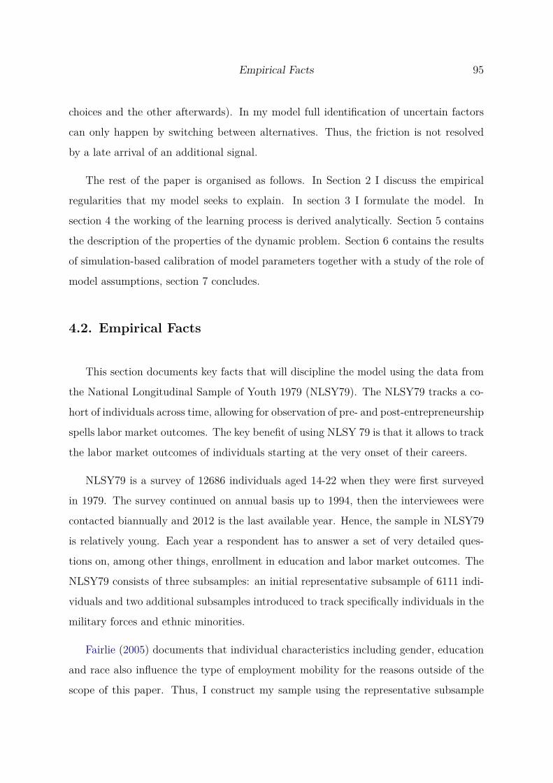
Empirical Facts 95
choices and the other afterwards). In my model full identification of uncertain factors
can only happen by switching between alternatives. Thus, the friction is not resolved
by a late arrival of an additional signal.
The rest of the paper is organised as follows. In Section 2 I discuss the empirical
regularities that my model seeks to explain. In section 3 I formulate the model. In
section 4 the working of the learning process is derived analytically. Section 5 contains
the description of the properties of the dynamic problem. Section 6 contains the results
of simulation-based calibration of model parameters together with a study of the role of
model assumptions, section 7 concludes.
4.2. Empirical Facts
This section documents key facts that will discipline the model using the data from
the National Longitudinal Sample of Youth 1979 (NLSY79). The NLSY79 tracks a co-
hort of individuals across time, allowing for observation of pre- and post-entrepreneurship
spells labor market outcomes. The key benefit of using NLSY 79 is that it allows to track
the labor market outcomes of individuals starting at the very onset of their careers.
NLSY79 is a survey of 12686 individuals aged 14-22 when they were first surveyed
in 1979. The survey continued on annual basis up to 1994, then the interviewees were
contacted biannually and 2012 is the last available year. Hence, the sample in NLSY79
is relatively young. Each year a respondent has to answer a set of very detailed ques-
tions on, among other things, enrollment in education and labor market outcomes. The
NLSY79 consists of three subsamples: an initial representative subsample of 6111 indi-
viduals and two additional subsamples introduced to track specifically individuals in the
military forces and ethnic minorities.
Fairlie (2005) documents that individual characteristics including gender, education
and race also influence the type of employment mobility for the reasons outside of the
scope of this paper. Thus, I construct my sample using the representative subsample

96 Confounded Entrepreneurial Choice
only and I focus on white men with at least some college experience. Furthermore, I
also remove farmers and workers from disadvantaged families. These data adjustments
serve the purpose of constructing a sample of ex-ante similar individuala, similar to the
approach of Papageorgiou (2013) to avoid blurring the type of employment mobility
patterns due to factors other than individual abilities. I consider an individual a worker
(either an entrepreneur or an employee) for a particular year if they reported income and
worked at least 400 hours in a given year and don’t report more than 60 hours worked
per week. Finally, I drop individuals with less than 3 observations on income as they
are the most likely to be mismeasured. In my sample I have 1080 individuals and 15083
observations. Income is defined as annual earnings, assigned to the job the respondent
reported working the most hours in a given year. An entrepreneurial spell (or spell in
short) is defined as a set of consecutive observations (at least one) in entrepreneurship
that ends with return to payroll employment or leaving the survey. Several stylised facts
can be identified.
Many workers try entrepreneurship and switch between activities. I find
that about 29 percent of workers have some entrepreneurial experience meaning they
have at least one observation in entrepreneurship. The first entry into entrepreneurship
usually happens in the early years of one’s career. About 45 percent of individuals
with some entrepreneurial experience have their first spell in the first five years after
entering the labor market as depicted on Figure 4.A.4. First entrepreneurial entry
after more than 10 years of labor market experience is very rare. Next, almost 40
percent of individuals who tried entrepreneurship are “serial” entrepreneurs, that is,
they have more than one distinct spell of entrepreneurship in their career separated by
periods of payroll employment. Thus, there is substantial type of employment mobility
among the young workers. These facts are demonstrated on Figure 4.A.3. Re-entering
entrepreneurship is most frequent among the earliest entrants. Interestingly, about two-
third of entrepreneurial spells are very short and last up to two years. These spells are
not limited to individuals who quit entrepreneurship and never return to it, they are also
prevalent among the serial entrepreneurs. The average time spent in entrepreneurship,

Empirical Facts 97
Table 4.1
Unconditional earningsNLSY 1979-2012, pooled data on white men, farmers, members of military and disadvantagedfamilies excluded. Income in thousands of 2012 dollars.
Entrepreneurs Employeesmean annual earnings 66.5 64.3median annual earnings 44.9 51.0std of annual earnings 72.2 57.8
conditional on having at least one spell, is 2.8 years which is about a sixth of average
individual history length.
Negative median earnings differential in entrepreneurship. The cross-sectional
distribution of annual earnings conditional on type of employment features larger disper-
sion of entrepreneurial income. The fatter right tail of entrepreneurial income drives the
mean enterpreneurial income up so that it exceeds, although only slightly, the mean of
employee income. The median entrepreneur earns about 12 percent less than a median
employee. The key characteristics of the pooled sample are described in Table 4.1 and
on Figure 4.A.1 the histograms of these distributions are provided.
To some extent, the income differentials may come from the timing of entrepreneurial
spells which for a large fraction of entrepreneurs happen at the early stage of their ca-
reers. Thus, the differential may be due, in particular, to human capital accumulation or
aggregate time-varying conditions. The earnings may also depend on the pre-entry char-
acteristics that determine the industry and occupation the individuals work at, including
the university degree etc. To remove the effect of observable factors in shaping the in-
come distribution I run a panel regression on log of annual earnings yit controlling for
observables Xit (labor market tenure, hours worked, years of education, degree obtained,
year fixed effect, industry) with an interacted individual type of employment fixed effect
βi × βei (t) which has βe
i (t) equal to 1 if an individual i at year t is self-employed and

98 Confounded Entrepreneurial Choice
zero otherwise:
yit = β0 + βXXit + βt + βind + βi × βei (t) + εit.
This approach, however, has some limitations given that for some workers with
shortest entrepreneurial spells it’s not possible to fully disentangle the fixed effect and
the individual independent shock (residual in the earnings regression). The histogram
of combined residual from the earnings equation including the individual fixed effect,
βiβet + εit, is provided on Figure 4.A.2. The residuals in entrepreneurship are more
dispersed. Then, to wash out the effects of observable characteristics I shift the residuals
to have the mean that corresponds to the mean of the log-earnings in the sample. By
converting back to levels it turns out that the median differential increases, the median
entrepreneurial earnings are 84 percent of median employee earnings. The ratio of the
means is roughly unchanged and stands at about mean entrepreneurial income being
larger by 2 percent.
Most early entrepreneurs earn less than what they could earn as employees.
Given the individual estimates of βiβet I can define under-performing entrepreneurs for
which it holds that the estimated βet < 0. The data on the subsample of workers with
at least 3 years of experience in either of the types of employment show that about
52 percent of entrepreneurs would earn more upon return to payroll employment. For
entrepreneurs with at least 5 years of experience this fraction drops to 36 percent. Thus,
it seems that the entrepreneurial learning is slow. However, this is difficult to reconcile
with large fraction of very short entrepreneurial spells. On the one hand, the first fact
implies that it is necessary to spend a lot of time as entrepreneur to correctly asses
the type of employment comparative advantage. On the other hand, the second fact
implies, at least at face value, that entrepreneurs efficiently learn about abandoning
entrepreneurship and quit fast. As my sample
Employee and entrepreneur earnings are positively correlated. After control-
ling for observable differences between agents the data show a positive correlation be-

Empirical Facts 99
Figure 4.1
Correlation of conditional payoffsIndividual averages of earnings condtional on observables in each type of employment for agentswith at least 3 observations in each of the activities.
50000 0 50000 100000 150000 200000 250000employee earnings
50000
0
50000
100000
150000
200000
250000
entr
epre
neur
earn
ings
tween earnings rank of employees and entrepreneurs. The location of an individual in the
earnings distribution of employees is similar to her location among entrepreneurs when
choosing that activity. The scatter plot of individual averages of income conditional on
observable characteristics for workers with experience in entrepreneurship and payroll
employment of at least 3 years is provided on Figure 4.1. The Spearman rank coefficient
is 0.67 and is significant at 1-percent level.
A priori there is no clear argument for correlation of any particular sign. For example,
it could be the case that business skills decline during formal education that increases
general ability. Then, if business skills were more important in entrepreneurship and
general ability more important in payroll employment, there should be a negative rank
correlation.
The evidence presented in this section poses some targets for the theory of en-
trepreneurial learning. First, the theory should be able to address how can the frequent
switches between entrepreneurship and payroll employment coexist with the large frac-

100 Confounded Entrepreneurial Choice
tion of underperforming entrepreneurs. In the baseline learning by doing model the en-
trepreneurs run their businesses and return to payroll employment only if their business
doesn’t perform as well as expected. Entrepreneurial learning has no frequent switching
back and forth between entrepreneurship and payroll employment. Second, the theory
should be able to generate sufficient incentives for experimentation in entrepreneurship,
reflected in the negative earnings differential, given the positive correlation of employee
and entrepreneurial incomes. For example, the latter fact suggests that the baseline
model should be extended with heterogeneity in the entrepreneurial outside option.
4.3. Basic Features of the Environment
In this section I introduce the key features of the entrepreneurial choice model which
is further expanded in the next sections. I also provide a short discussion of the assump-
tions implicit in the model formulation.
Preferences and Technology.
The economy is inhabited by a unit mass of individuals who value their consumption
ct and have utility function u (ct). There is no storage of the consumption good so that
the production within period yt is consumed fully. All individuals live for T periods.
The size of the population is kept constant as new generations enter the economy and
the size of each population is constant and equal to 1T
. The agents discount the future
at a rate β.
There are two types of income generating activities: entrepreneurship and payroll
jobs. Each individual i has some endowment of general ability a∗i and business acumen
m∗i . The endowment of (a∗
i , m∗i ) is distributed in the economy according to a distribution
function F (a∗i , m∗
i ), bivariate normal with parameters {µa∗ , µm∗ , σ2a∗ , σ2
m∗ , ρ∗}. The indi-
viduals may opt out from productive activities choosing not to participate in the labor
market and enjoy a value of leisure of b which can be thought of as home production
that does not require any specific skills.

Basic Features of the Environment 101
The production function is type of employment (p for payroll and e for entrepreneur-
ship) specific and is subject to idiosyncratic productivity shocks εpi,t, εe
i,t which volatilities
σ2p and σ2
e can depend on the type of employment1. The agents supply their ability and
acumen inelastically. Most importantly, income in entrepreneurship can, in general,
depend on both general ability and acumen while payroll income is postulated to be a
function of a∗i . Formally:
ypi,t = a∗
i + εpi,t, where ∀i εp
i,t ∼ N(0, σ2
p
), (4.1)
yei,t = γa∗
i + m∗i + εe
i,t, where ∀i εei,t ∼ N
(0, σ2
e
), (4.2)
yni,t = b. (4.3)
The parametric specification of production in entrepreneurship features an additional
parameter γ which scales the effect of general ability on entrepreneurial income. γ is
assumed to be in the [0, 1] interval. This implies that there are some gains from higher
ability in entrepreneurship on top of the business acumen and that for agents with low
acumen the payroll employment dominates entrepreneurship.
Information friction
The individual ideas and abilities are not observable and can only be learned by
observing production. Hence, the entrepreneurial income constitutes a confounded signal
on the pair (a∗, m∗) whenever γ > 0. The entrepreneur faces an identification problem
learning from one signal about two unobservables. All agents at time of birth receive
an initial unbiased signal about true abilities (a∗, m∗). The signal produces individual
agent’s prior about her composition of abilities Ii,0, bivariate normal with parameters{ai,0, mi,0, σ2
a,i,0, σ2m,i,0, ρi,0
}.
Intuition for the role of γ and ρ
Observe that the special case of γ = 0 and ρ∗ = 0 implies that individual em-
ployee and entrepreneurial incomes are uncorrelated and each provides a signal on one1The equations (4.1)-(4.2) will describe either the level or log of product, depending on the context.

102 Confounded Entrepreneurial Choice
dimension of unobservable heterogeneity. In that case the model developed here can be
considered a version of the Jovanovic model of entrepreneurial learning, extended with
learning about the outside option of payroll income.
Unconditionally, these two parameters can’t be jointly identified without the knowl-
edge of the initial distribution of the beliefs, as both introduce observationally some
correlation between the individual payoffs in the two types of employment. However,
if a consistent estimate of the distribution of individual ability a in the population is
available, one can disentangle the two. Without loss of generality, I will only consider
parametrisations that produce positive correlation of individual payoffs in the two types
of employment.
First, let there be γ = 1 but ρ > 0. This implies that the entry rates into en-
trepreneurship increase while exit rates decrease with increasing employee earnings and,
on top of that, the highly skilled employees also enjoy an increasing comparative ad-
vantage in entrepreneurship. On the other hand, let ρ = 0 but γ < 1. This means
that the entry rate in entrepreneurship falls with ability but the distribution of com-
parative advantage in entrepreneurship is negatively correlated with employee earnings
(because γ < 1) and the correlation decreases towards the left tail of employee earnings
distribution.
The dynamic problem
The decision problem the worker is facing is to choose an action plan ξT = (ξ1, ..., ξT )
that contains the decision to work in entrepreneurship, in a payroll or to remain out of the
labor force. The actions ξt thus are in the discrete set Ξt ∈ {ξe, ξp, ξn}. Each action plan
ξt generates a set of all possible income realization histories St with a typical element
being the history of production yt = (y1 (ξ1) , ..., yt (ξt)). A priori, the plan is conditional
on all future possible realizations of income. The optimization problem P that the
households solve is given below, the dependence on all model-relevant parameters is
omitted for convenience.

Basic Features of the Environment 103
P : max{ξt(It)}T −1
t=0
V = EI0
T −1∑t=0
βtu (yt (ξt (It))) subject to:
belief updating: It = f(It−1, yt−1
), given I0
and the production function.
One can think of P as of an agent choosing an action plan for all possible states of
the world captured in her beliefs, or making the decision sequentially. Observe that P is
an example of a multi armed bandit problem (MBP) with bandit arms corresponding to
choices of activity. Unless γ = 0 and ρ∗ = 0 the payoffs ypi,t and ye
i,t are not independent.
Either because of the lack of independence of arms or the finite horizon (or both)the
problem P does not meet the criteria for applicability of the standard approach of index
policies proposed in Gittins (1979). It means that it is not possible to decompose the
problem of choosing between M arms into M one-dimensional problems and solve them
forward. The exact solution has to make use of M -dimensional dynamic programming
techniques. Following the standard approach in the literature on MBPs, I work with the
expected Bayesian regret2. Intuitively, the regret is a measure of the cost of uncertainty
about the optimal (in expectations) course of action.
Definition 4.1 (Bayesian regret). Let ξ∗t be the optimal arm in period t. The expected
Bayesian regret R is:
R = EI0
T −1∑t=0
βt [u (yt (ξ∗t )) − u (yt (ξt))] . (4.4)
Observe that minimization of the discounted sum of expected Bayesian regret yields
identical policy as the one that solves P . As the optimal arm in each period is fixed
and doesn’t depend on the action plan ξT , we can decompose the sum in equation (4.4),
as the returns to the best arm V and the target function V in problem P so that2An alternative is an approximate algorithm that employs an idea similar to the maximum likelihood
test, proposed by Brezzi and Lai (2002). A popular reference on Bayesian regret is Bubeck and Cesa-Bianchi (2012).

104 Confounded Entrepreneurial Choice
V (It) = V −R (It). From this relationship it follows that maximizing V is equivalent to
minimizing R. Intuitively, the choices the agents make affect their future information set
and the incoming information is used in the decision making. I start with a description
of the learning process, the analytical characterization of the regret follows.
4.4. Learning
The goal of this section is to build insight on the consequences of the structure of
the signals and describe the dynamics of the evolution of the beliefs, It = f (It−1, yt−1).
Without loss of generality let’s consider an agent of age t ≤ T . We consider an action
plan ξT and some particular history of production st =(yp
1, ..., yptp
, ye1, ..., ye
te, b1, ..., btn
)without taking stand about its optimality. A key feature of history st is how much time
was spent not producing tn ≥ 0 or producing either in payroll employment tp ≥ 0 or in
entrepreneurship te ≥ 0 with ti = ∑1ξt=ξi . Naturally, any such partition exhausts st in
the following sense:
t − tn = tp + te. (4.1)
The following two results can be shown with the proof relegated to Appendix 4.B.
Proposition 4.1 (Sufficient statistic). The sufficient statistic for It given I0 is {yp, ye, te, tp}
with yk = 1tk
∑tkl=0 yk
l , the sample mean.
Proposition 4.2 (No learning when not producing). Let ξt = ξn, then It = It−1.
The proposition 4.1 permits the use of standard dynamic programming techniques, in
line with the results in chapter 10 of Bertsekas and Shreve (2007), including a recursive
representation of the dynamic problem. Theorem 4.1 characterizes the belief It as a
function of initial beliefs and history st, the dependence of the beliefs on agent’s index
i is omitted for convenience.

Learning 105
Theorem 4.1. Consider an agent with an initial belief I0 with a type employment history
st summarized by a sufficient statistic (te, tp, yp, ye). Let’s introduce3 the uncertainty
reduction scaling factors:
ησ2e
(te, tp) = te
σ2e
+ 1(1 − ρ2
0) σ2m,0
ησ2p
(te, tp) = tp
σ2p
+ γ2te
σ2e
+ 1(1 − ρ2
0) σ2a,0
,
the confounding correction factor:
κ (te) = ρ0
(1 − ρ20) σa,0σm,0
− γte
σ2e
,
and the posterior mean updates:
ϕa∗ (tp, te, yp, ye) = tpyp
σ2p
+ γteye
σ2e
+ a0
(1 − ρ20) σ2
a,0− ρ0m0
(1 − ρ20) σa,0σm,0
ϕm∗ (tp, te, yp, ye) =(
teye
σ2e
+ m0
(1 − ρ20) σ2
m,0− ρ0a0
(1 − ρ20) σa,0σm,0
).
Then, the belief It has:
– posterior means:
at =ϕa∗ησ2
e+ ϕm∗κ
ησ2pησ2
e− κ2
mt =ϕm∗ησ2
p+ ϕa∗κ
ησ2pησ2
e− κ2
– posterior variances:
σ2a,t =
ησ2e
ησ2pησ2
e− κ2
σ2m,t =
ησ2p
ησ2pησ2
e− κ2
– and the correlation coefficient:
ρt = κ√
ησ2pησ2
e
3I scrap the dependence of those on the model primitives only the role of sufficient statistic is keptvisible.

106 Confounded Entrepreneurial Choice
Observe that only with γ = 0 the confounding factor κ has a non-vanishing effect
on posterior beliefs (there is some effect coming from ρ0 but it vanishes asymptotically).
Next, one can show that the standard property of rational updating holds, namely that
the belief means at and mt are martingales. Thus, the agents don’t expect any drifts in
their beliefs.
Theorem 4.2 (Martingale property of beliefs). Take a belief It with some at, mt and
history st with te, tp = 0. It holds that
∀ξt+1 Etat+1|It = at and Etmt+1|It = mt.
Asymptotic beliefs
Now, for illustrative purposes let’s consider an extreme situation of indefinitely long
learning for an agent with life length T 7→ ∞. To contrast the model developed here
with the baseline learning model I start with an assumption that the agents choose their
type of employment once-and-for-all at birth. For convenience let γ = 1.
Corollary 4.1 (Asymptotic beliefs, fixed type of employment.). Let γ = 1. Consider
the infinite horizon updating problem of an agent with true individual abilities bundle
(a∗, m∗). Then the limiting belief distribution satisfies:
– in payroll employment:
limt 7→∞
at = a∗ limt 7→∞
mt = m0 + ρ0σm,0
σa,0(a∗ − a0)
limt 7→∞
σ2a,t = lim
t 7→∞ρt = 0 lim
t 7→∞σ2
m,t =(1 − ρ2
0
)σ2
m,0
– in entrepreneurship:
limt 7→∞
at =(a∗ + m∗)
(1
σ2m,0
+ ρ0σa,0σm,0
)+ a0
σ2a,0
− m0σ2
m,0+ ρ0
σa,0σm,0(a0 − m0)
1σ2
a,0+ 1
σ2m,0
+ 2ρ0σm,0σa,0
,

Learning 107
limt 7→∞
mt =(a∗ + m∗)
(1
σ2a,0
+ ρ0σa,0σm,0
)− a0
σ2a,0
+ m0σ2
m,0+ ρ0
σa,0σm,0(m0 − a0)
1σ2
a,0+ 1
σ2m,0
+ 2ρ0σm,0σa,0
,
limt 7→∞
σ2a,t = lim
t 7→∞σ2
t = 1 − ρ20
1σ2
a,0+ 1
σ2m,0
+ 2ρ0σm,0σa,0
,
limt 7→∞
ρt = −1
Thus, an agent that spends the entire career as an employee can consistently estimate
a∗ and remove uncertainty about it completely. The correlation coefficient of beliefs on
a∗ and m∗ goes to zero as the prior belief I0 is dominated by an infinite sequence
of payroll income signals that have no correlation with m∗. If there’s some correlation
between (a∗, m∗) then the employee career provides additional insight about the business
acumen. Otherwise the agent learns nothing about m∗ on top of the information in the
prior distribution. The correction of m0 is the linear projection of the data on the initial
beliefs.
The entrepreneur can identify her skill bundle up to a line on the (a∗, m∗) plane
with -1 slope on which the limiting belief is bivariate normal distributed. The negative
correlation in the limiting belief comes from a∗ and m∗ being complements to each
other in entrepreneurship. The mass is symmetrically (as indicated by asymptotic m
and a variances) centered around the confusion-adjusted point (limt 7→∞ at, limt 7→∞ mt).
The confusion adjustment factor is a function of uncertainty-adjusted initial information
about one’s abilities. Whenever either a0 = a∗ or m0 = m∗ the entrepreneur can not
consistently estimate her endowment. This is contrary to the payroll employment case
where the limiting belief on a∗ is consistent irrespectively of prior information.
Observe, however, that the entrepreneur updating problem allows for consistent es-
timation of the individual entrepreneurial return, exactly as in the Jovanovic model, as
by taking the sum of the limits we get:
limt 7→∞
at + limt 7→∞
mt = a∗ + m∗.
Because of the confounding nature of the signal the prior information constantly weighs

108 Confounded Entrepreneurial Choice
in on the estimates of the means of both unobservable factors. If an agent believes
that her acumen/ability is higher than its true value, then this decreases the mean of
the ability/acumen, respectively, in the updated belief. Thus, it may not be possible
to infer the value of the outside option as individual ability and the business acumen
jointly determine entrepreneurial income. The magnitude of the confusion effect hinges
on the quality of initial information. To see why this is the case consider the rewritten
formulation of the asymptotic belief about the business acumen limt 7→∞ mt under an
additional simplification of ρ0 = 0:
limt 7→∞
mt =σ2
m,0
σ2m,0 + σ2
a,0(a∗ − a0) +
σ2m,0
σ2m,0 + σ2
a,0m∗ +
σ2a,0
σ2m,0 + σ2
a,0m0. (4.2)
Equation (4.2) is vital to understanding the implications of the model. The belief is a
weighted sum of the prior information m0 and the true value m∗ shifted by the rescaled
error on the general ability a∗. Thus, there are two factors that make agents value
entrepreneurship above payroll employment even if the evidence points to a∗ + m∗ < a∗.
First, agents that have initial belief on their general ability below its true value will
tend to have better opinion about their business acumen. Second, a similar effect has
an initial overestimation of m∗.
Next, the more precise the estimate of the general ability, the smaller the interference
of ability on the belief on acumen due to the confounded nature of the entrepreneurial
learning. In particular, it follows that:
limσ2
a,0 7→0limt 7→∞
mt = m∗,
as in the baseline model. However, this discussion depends to some extent on the
assumption of fixed careers, as the following corollary demonstrates.
Corollary 4.2. If te = tp and tp + te = t 7→ ∞, then the asymptotic beliefs have:
limt 7→∞
at = a∗ limt7→∞
mt = m∗
limt 7→∞
σ2a,t = lim
t 7→∞ρt = lim
t 7→∞σ2
t = 0

Illustration of the working of the model 109
Hence, the agents can refine their belief on the business acumen by switching between
the two types of employment. Payroll employment experience is necessary to recover
the true value of business acumen. Now we are in position to characterize the regret
function and to solve the dynamic problem P . Before we do that, however, I will provide
more intuition for the consequences of one of the key ingredients of confounding, the
individual uncertainty about one’s ability.
Intuition for the consequences of uncertain individual ability
If we were to assume that every agent knows her ability a∗, the model would become
a variant of Jovanovic model. There the negative premium to entrepreneurship may
occur (meaning that the median entrepreneur will earn significantly less than a median
employee) if there is a large mass to the left of the entry threshold in the distribution
of entrepreneurial ideas and the right tail is relatively thin.
However, a model with a certain and safe return to payroll employment can not
generate persistence of the negative premium to entrepreneurship (relative to employee
earnings) over longer tenures in running a business venture. Thus, because of this
“Darwinian selection” feature, such models can’t match the findings of Hamilton (2000)
whereas the model with confounding can.
4.5. Illustration of the working of the model
In this section the analytical properties of the regret function are derived. Then,
the dependence of the dynamics of type of employment choice on model parameters
is discusssed in a 3-period setting. Unless stated otherwise, the earnings process is
considered to hold in levels of income and the utility is linear. To begin with, I provide
the solution to the dynamic problem P sans information friction.

110 Confounded Entrepreneurial Choice
Choice in the absence of information friction
As we have three choices and the composition of the ability-acumen endowment is
fixed, one choice is optimal in all periods and the optimal action plan sequence {ξ∗1 , ξ∗
2 , ξ∗3}
satisfies:
∀t ∈ {1, 2, 3} : ξ∗t =
ξp if max{b, γa∗ + m∗} ≤ a∗
ξe if max{b, a∗} ≤ γa∗ + m∗
ξn otherwise.
When the endowments are unobservable and can only be learned by producing, the
individual outcomes will differ from the perfect information case.
Baseline regret function: no opportunity cost of ability
For ease of exposition I start with a somewhat special parametric case, focusing first
on the choice between the two types of employment by putting b = −∞. This rules out
non-participation as a valid choice for the agents. I also fix γ = 1 so that the returns
to general ability are identical in the two activities. The opportunity cost of switching
between the activities is the value of agent’s business acumen, m∗i . It is also assumed
that ρ∗ = 0 so that refining the precision of information on a∗i does not provide additional
information on m∗i . Then, the definition of the regret within a particular period t is:
R (It, ξt) =
PIt (m∗ > 0)EIt (m∗|m∗ > 0) if ξt = ξp
PIt (m∗ < 0)EIt (−m∗|m∗ < 0) if ξt = ξe
(4.1)
Observe that the regret is an expectation of a truncated normal variable with pa-
rameters m, σ2m weighted by the probability of a tail event of m∗ being either below or
above zero. Thus, the analytical representation of the regret in period t is:
Et [y (ξ∗) − y (ξt) |It] =
(1 − Φ
(− mt
σm,t
))mt + σm,tϕ
(− mt
σm,t
)if ξt = ξp
−Φ(− mt
σm,t
)mt + σm,tϕ
(− mt
σm,t
)if ξt = ξe

Illustration of the working of the model 111
Proposition 4.3 (Regret dependence on It.). Let b = −∞, ρ = 0, γ = 1, then the
regret is increasing in σ2m. The minimum of the regret is decreasing in |m|. The regret
does not directly depend on a, σ2a.
The regret of each arm is a convex function of the mean of individual belief on m∗,
as demonstrated on Figure 4.A.5. The minimum envelope of the regret is always non-
negative, has a maximum at mi = 0 which is the threshold for the change of arm, and
decreases to zero the more extreme the values of the mean of the beliefs on m∗i . In
other words, the more convinced agents are about their advantage in one of the types
of employment, the less likely they expect themselves to choose the wrong arm ex ante.
This is the exploitation motive in the agent’s optimization problem. The arm that seems
to generate a higher reward is more desirable to choose.
Regret is also increasing in uncertainty on m∗ which reflects the experimentation
motive. Getting rid of uncertainty is valued because it decreases the probability of
choosing the wrong arm given all other available information. The impact of decreasing
uncertainty diminishes the more extreme means of the beliefs are. Hence, the more
extreme the mean of the belief about the acumen, the smaller is the expected gain from
learning. Intuitively, the more extreme the belief on m∗ is, the less the agents expect to
be wrong about m∗ which makes the gains from reducing uncertainty about it smaller
than for the beliefs near the m = 0 switching threshold.
Knowledge of a∗ plays no role in this formulation as the choice of ξt = ξe does not
entail any losses of the true ability a∗ which only holds when γ = 1. In this case the
uncertainty on a∗ can only create additional (on top of initial uncertainty about the
acumen) confusion about m∗ and interact with the pace of uncertainty reduction on m∗.

112 Confounded Entrepreneurial Choice
The role of ρ, γ and non-participation.
Now, let’s allow 0 ≤ γ < 1 and −1 < ρ < 1 keeping b = −∞. Observe that in this
case the regret definition is:
R (It, ξt) =
(1 − PIt (m∗ < (1 − γ) a∗))EIt (m∗ + (γ − 1) a∗|m∗ > (1 − γ) a∗) if ξt = ξp
(1 − PIt (m∗ > (1 − γ) a∗)EIt ((1 − γ) a∗ − m∗|m∗ < (1 − γ) a∗)) if ξt = ξe
This can be rewritten introducing a new variable z∗ = m∗ − (1 − γ) a∗ which is
distributed as univariate normal with mean z = m − (1 − γ) a and variance σ2z = σ2
m +
(1 − γ)2 σ2a + 2ρ|γ − 1|σaσm. Then, one can rewrite the regret equation (4.1) using z
and σz instead of m and σm. In that case the proposition 4.3 extends naturally to z∗.
The minimum of the regret is decreasing in the belief on the ability-adjusted individual
advantage in entrepreneurship |z|. The regret increases with σz. This fact is further
illustrated on Figure 4.A.6 with changes in σa now translating in different values of
regret, contrary to Figure 4.A.5.
Thus, having γ = 1 introduces a motive for learning a∗. This comes from the fact
that now the agents advantage in entrepreneurship is a function of ability as well and
the agents may make mistakes due to imperfect identification of the switching threshold
m∗ = (1 − γ) a∗.
Finally, non-participation is an absorbing state. In other words, when b > −∞,
if an agent chooses ξt = ξn the subsequent periods will have ξt+k = ξn, k > 0. The
intuition behind this result is as follows - agents with beliefs that imply their value of
home production exceeds their value of productive activities can still decide to begin
their career producing solely for the sake of learning. The benefits of learning are
decreasing with agent’s experience thus if they don’t justify undertaking production
in period t, they will also not be big enough to make the agent produce in all future
periods. However, because of this property of non-participation the agents have strong
incentives to improve the finesse of their estimates of ability and acumen before leaving
the labor market. The introduction of non-participation also implies that the optimal

Illustration of the working of the model 113
choice is not only driven by the comparative advantage between the two productive
abilities, z∗. Because of non-participation, location of agent’s beliefs in (a, m) space is
also relevant for the dynamics.
Dynamics of Type of Employment Choice
Let’s again assume that b = −∞ so that the choice is between two productive arms
only. Deriving the optimal decision rule is easiest for the last period. Observe that for
t = 0, 1, 2 the following identity holds:
R (It, ξt = ξp) − R (It, ξt = ξe) = z.
Hence, in the final period the optimal decision is to choose the e-arm when m2 >
(1 − γ) a2 and p-arm when m2 < (1 − γ) a2, breaking the tie arbitrarily. This reflects
the fact that in a one-period setting there is no value from experimentation, solely the
exploitation motive is present. To put it simply, the benefits of reducing uncertainty
today are only available in the next period which is absent when t = 2. In the first two
periods wtih t = 0, 1, however, there is the experimentation gain, namely the decrease of
regret coming from the reduction in σ2z which may dominate the current-period increase
of regret from choosing a suboptimal arm. From the fact that the decrease of the regret
function due to reducing σz diminishes with |z| the following result naturally follows.
Observation 4.1 (Reservation property). Consider an agent with belief It with some
zt. If it is optimal for this agent to choose ξt = ξe then it is also optimal to choose
ξt = ξe for all agents with posterior It such that zt ≥ zt other things equal.
Informational gains
In the first and second period the agents may opt for choosing an inferior arm to
decrease their uncertainty about the (a∗, m∗) pair. The size of those informational
benefits depends, however, on the signal to noise ratio in both types of employment
and initial uncertainty. Intuitively, the more uncertain agents are about one of their

114 Confounded Entrepreneurial Choice
endowments, the greater the incentive to experiment. The more noisy an activity is, the
less desirable a choice for learning it represents. The more correlated are the individual
beliefs, the smaller the relative difference in informational gains of the two choices shall
be.
An additional source of complexity is that the use of ability and acumen in en-
trepreneurship yields some information on both endowments, yet in a confounded way.
On the one hand, entrepreneurship brings informational gains on both components of
zt. On the other hand, informational gains of choosing entrepreneurship in consecutive
periods decrease faster than in payroll employment as there are limits to learning in
entrepreneurship.
For the magnitude of the informational gains the relative initial uncertainty and
signal to noise ratios in the two activities are key. Thus, let’s have all the variances
σ2m,0, σ2
a,0, σ2p, σ2
e normalised to one to investigate the role of γ and ρ∗. On Figure 4.A.7
the reduction of uncertainty about z∗ is presented, measured as the ratio of period-1
variance of the z estimate to its initial variance. On Figure 4.A.8 the same measure
after two periods is plotted. In each case, the informational gains depend on the choices
the agents made.
In the noisy learning case the initial period informational gains are identical, as the
uncertainty about both unobserved endowments and the noise-to-signal ratios are the
same. This is not the case in the initial period in the confounded learning case. There,
for larger values of γ entrepreneurship dominates informationally payroll employment.
This is because the uncertainty about m∗ weighs more in the overall uncertainty about
z∗. Only when γ goes to zero, the relative informational advantage of entrepreneurship
vanishes.
In the second period, using each arm once produces uniformly largest informational
gase n the noisy learning case. If there is confounding, however, this is not always the
case. In particular, for large values of γ choosing entrepreneurship twice may informa-
tionally dominate other choices. What is more, choosing entrepreneurship twice and in

Illustration of the working of the model 115
particular, switching between occupations dominates the choice of payroll employment
in the first two periods to a significantly larger extent when γ > 0 than in the noisy
learning case.
The magnitudes of the effects described above depend to some extent on the desire
to experiment about entrepreneurship, expressed as a ratio of initial beliefs σ2m,0
σ2a,0
and the
speed of learning in each activity measured by the signal to noise ratio. To fix ideas,
let’s keep σ2a,0 = σ2
p = 1. Then, by increasing σ2m,0 the incentives to learn about m∗
increase. These incentives are diminished when variance of shocks to entrepreneurial
income increases. However, the interaction of the two effects can be non-trivial. As
demonstrated on Figures 4.A.9 and 4.A.10, with σ2m,0 increased twofold and σ2
e increased
threefold, the informational gains of entrepreneurship in the confounded learning case
increase in the first two periods while they decrease in the noisy learning case.
Reservation thresholds
For illustration of trade-offs in the dynamic problem, two cases are considered, strong
correlation (ρ = 0.8, γ = 0) in a noisy, confounding-free setting and strong (γ = 1,
ρ∗ = 0) confounding, labelled NL and SC respectively. The assumption of all relevant
variances normalised to one made at the beginning of the previous section is maintained.
In line with lack of the experimentation motive, in the last period the switching threshold
in all cases is at z2 = 0.
Let’s start with the noisy learning case. As in the first period both arms offer identical
learning benefits, the agents have no experimentation motive to prefer one arm over the
other. Thus, the switching threshold is zNL0 = 0. In the second period agents have
an experimentation incentive to switch. This incentive is identical in the case of initial
period entrepreneurs and employees given the symmetry of all relevant variances. The
individuals who started as employees are now willing to try entrepreneurship provided
their estimate of z1 is not too low. The same holds for first period entrepreneurs, who
are willing to give away some benefits of entrepreneurship. Thus, we obtain the following

116 Confounded Entrepreneurial Choice
set of conditions:
zNL0 = zNL
2 = 0 ∧ 0 > zNL1 (ξ0 = ξp) = −zNL
1 (ξ0 = ξe) .
Now, in the confounding case there are strong incentives to identify m∗ which domi-
nate analogous incentives to identify a∗. In line with the results on informational gains,
it holds that z0SC < 0. Then, the first-period employees will have an incentive to switch
into entrepreneurship for some z1 (ξ0 = ξp) < 0. The first period entrepreneurs have
no incentives to switch as the learning via switching and continuation provide identical
relative information gains. Thus, in the strong confounding setup we have:
zSC1 (ξ0 = ξe) = zSC
2 = 0 ∧ 0 > zSC1 (ξ0 = ξp) > zSC
0 .
Thus, keeping initial uncertainty constant, the increases in γ yield larger experimen-
tation incentives via entrepreneurship and increase the fraction of shorter entrepreneurial
spells compared to changes in the correlation of beliefs. This comes from the difference
between zSC1 (ξ0 = ξe) − zSC
0 . The switching tresholds are depicted on Figure 4.A.11.
4.6. Quantitative Analysis
This section starts with the description of the numerical simulation procedure that
pins down the parameters of the model. Then, I investigate the implications of introduc-
ing non-pecuniary benefits of entrepreneurship and the role of non-participation margin.
The learning model has γ > 0 which makes entrepreneurial learning confounded, the
ability and acumen are independently distributed. Finally, I use the parameter values
for the confounded entrepreneurial learning specification and conduct an experiment on
the impact of the reduction of uncertainty of the initial prior on the general ability.
Simulation based estimation setup
I employ Simulated Method of Moments (SMM) to pin the parameters of the model.
The preferences are logarithmic, u (c) = log (c) and the production equations are as-
sumed to hold in logs of product. Observe that this yields the regret function analogous

Quantitative Analysis 117
to the level-level case in expected utilities. Thus, agents seek to minimize the distance
to the arm offering highest expected utility.
Because there is substantial evidence that pre-retirement considerations, health and
technological changes interact with type of employment choice of older workers, I assume
that agents in my model have in total 30 periods/years to choose their activity and then
stay on this activity until retirement after 40 years since entering the labor market.
This assumption is due to that in later age the learning motive may be dominated by
aforementioned factors.
The sole externally calibrated parameter is the discount factor β set to 0.96. The
parameters of interest include the parametrization of F (a, m), the precision of initial
beliefs, the variance of idiosyncratic shocks σ2p and σ2
e and the value of non-participation
b. Then, I assume that acumen and ability are independent, ρ∗ = 0 and allow γ to vary.
Below I provide a discussion of identification of each of the parameters.
The primary source of targets for the simulations are the moments of the log-residuals
from the earnings equation. In particular, the targets include the standard deviations
of those residuals and standard deviations of individual averages of the residuals, all
conditional on type of employment. These four distributions provide natural targets for
σ2a∗ , σ2
m∗ and σ2p, σ2
e .
As the choice of productive activities works is driven by relative returns, I normalise
the mean of the general ability in the population µa∗ to zero. To compare the model with
the data I then shift the log-residuals to produce the same mean log-residual earnings in
payroll employment. Then, conditionally on the standard deviations of ability, acumen
and individual shocks the mean of the business acumen distribution µm∗ is matched by
a restriction of the ratio of the means of the two income distributions. The level of
initial uncertainty about ability is matched exogenously to the noise variance in payroll
employment so that an agent who never tries entrepreneurship learns the ability at the
end of the 30-year period4. The identification of uncertainty on individual business4An alternative calibration strategy would have the value of non-participation calibrated from the

118 Confounded Entrepreneurial Choice
acumen relies on the desire to experiment between the productive activities as relative
informational gains are a function of relative uncertainty on m∗ and a∗. Thus, I target
the entrepreneurship rate in the cross section which is decreasing in initial uncertainty,
given all other parameters of the model.
The untargeted moments consist of the features of the data that will be driven by the
learning process. Those include the distribution of spells and switches, the differential
of median earnings of entrepreneurs and employees in the cross-section and the fraction
of underperforming entrepreneurs among the individuals with 10 years of labor market
experience, frequency of returns to entrepreneurship after the first spell. The model is
solved in the space of beliefs on a grid that approximates the F (a, m) distribution. The
description of the numerical algorithm is relegated to Appendix 4.C.
Learning, non-pecuniary benefits and non-participation.
I estimate the parameters of the baseline model and then I re-estimate the parameters
considering the role of several features of the model. To this end, I test the importance
of the lack of separate observation of ability and acumen in entrepreneurship (with γ = 0
but two separate signals on a and m) and the role of non-participation. The results of
this exercise are represented in Tables 4.1 - 4.2. The model is able to match most of
the targeted moments relatively well, as demonstrated in the Table 4.1. Due to strong
experimentation motives, both against non-participation and payroll employment, the
cross-sectional entrepreneurship rate is slightly above and non-participation rate is below
those in the data.
For the untargeted moments (Table 4.2), the model is able to generate negative
median earnings differential, although a bit less than a half (6 percent) of the magnitude
of the differential (16 percent) in the data. The model replicates about 90 percent of
the magnitude of short spells pointing to high exit rates from entrepreneurship. The
estimated parameters are presented in Table 4.A.1.
literature as a function of average employee income which would allow the uncertainty on the generalability to vary.

Quantitative Analysis 119
Table 4.1
Effects of confounding and non-participationSMM implied targeted moments (reestimated for each).
Targeted Moments data model no confounding no non-partic.
σ(log
(yp
i,t
))0.73 0.71 0.73 0.73
σ(log (yp
i ))
0.60 0.59 0.60 0.61σ(log
(ye
i,t
))1.08 1.07 1.16 1.14
σ(log (ye
i ))
0.83 0.86 0.92 0.64corr
(log
(yp
i,t
), log
(ye
i,t
))0.68 0.65 0.29 0.60
ratio of mean incomes entr.emp. 1.02 1.04 1.03 1.05
non-participation rate 0.10 0.08 0.07 –cross-sec. entrepreneurship rate 0.06 0.10 0.19 0.10
Table 4.2
Untargeted moments and the role of model assumptions
Untargeted Moments data model no confounding no non-partic.ratio of medians entr.
emp.0.84 0.94 0.86 0.96
frac. of underpeforming entr. 0.36 0.32 0.20 0.22share of serial entrepreneurs 0.39 0.51 0.06 0.76ever trying entrepreneurship 0.29 0.71 1.00 0.88share of 1-2 p. spells in entr. 0.68 0.54 0.04 0.42share of entries with 0-5 experience 0.41 0.65 1.00 0.86entr. rate up to 5 yrs. of activity 0.03 0.45 0.86 0.49
Let’s start with the analysis of the true skills space which are depicted on Fig-
ure 4.A.12. There are three blue lines which demark six regions in the parameter space.
First, there is the a∗ = b line which separates the beliefs that point to payroll employment
being better/worse than non-participation. Second, there is a line m∗ = (1 − γ) a∗ that
separates the beliefs that imply entrepreneurship dominating/being dominated by pay-
roll employment. Finally, the lne m∗ +γa∗ = b separates the regions of non-participation
being better/worse than entrepreneurship.

120 Confounded Entrepreneurial Choice
Then, the implied distribution of initial begins is presented on Figure 4.A.13. In the
regions R1 and R6 the incentives to choose entrepreneurship are the strongest. These
beliefs are likely to have the acumen overestimated, as indicated by the comparison of
the corresponding regions on the true types distribution plot. The regions R4 and R5
imply that the agents should leave the labor market. In those two regions experimen-
tation determines the behavior of agents until they learn better their underlying type
or indeed leave the labor market. Those two regions generate additional entrepreneurial
spells. In the last two regions R2 and R3 can only suffer from some of the high-quality
entrepreneurs choosing payroll employment.
The dynamics of the model are such that at early age the experimentation thresholds
shift in favor of entrepreneurship which provides information on a∗ and m∗. This is
responsible for a counterfactual prediction of the model on the share of entrepreneurs
among the agents with tenure in the labor market no longer than 5 years which well
exceeds the low entrepreneurship rate in the data. However, this is a mechanical feature
of the model as the young workers have the strongest incentives to experiment and that
there are no entry restrictions in entrepreneurship. Imposing a random idea arrival rate
would solve this problem but it would also require tracking the full history of ideas
agents have tried leading to an increase of the state space size. On the other hand, that
also means the potential of confounding is diminished and, in line with the discussion of
this issue in the introduction, the median differential reported here constitutes a lower
bound of the difference if one was to consider multiple ideas etc. Thus, the entry rate into
entrepreneurship is too high in the model, as reflected by the share of agents who ever
tried entrepreneurship. However, the size of this discrepancy is most likely overstated
in the model, as the shortest entrepreneurial spells are likely to be under-represented in
the sample.
The assumption of confounded signal is an important one. The model with sepa-
rate observation of the two underlying dimensions of individual heterogeneity although
also able to generate the negative median income differential, predicts an even larger

Quantitative Analysis 121
entrepreneurship rate and completely misses the features of the entrepreneurial spells
distribution. For example, the exit rate in the first two years is by a factor of ten smaller
than the corresponding moment in the data. There are fewer serial entrepreneurs. Those
predictions of the model are a consequence of too great an informational advantage of
entrepreneurship. Essentially all agents try entrepreneurship at their early age and stay
for several years before they efficiently learn what type of employment suits them best.
The role of non-participation is less trivial. Certainly, it decreases the exit rate from
entrepreneurship by one-fifth. The cross-sectional cost of experimentation decreases be-
cause there is one less activity available for the agents, now relatively fewer highly-skilled
agents select into entrepreneurship. The non-participation in the baseline model was re-
moving mostly least skilled employees so that the median negative earnings differential is
larger than for the baseline model and gets closer to unity as the distribution of employee
earnings has more mass to the left.
Then, using the estimated values of the model parameters I introduce non-pecuniary
compensation in entrepreneurship to match exactly the median differential between en-
trepreneurial and employee incomes. As expected and demonstrated in Table 4.A.3, the
frequency of switches between the two activities decreases and the entrepreneurship rate
goes up.
Cost of uncertainty and the effects of reducing uncertainty.
Based on the estimated values of the parameters I check the effects of an exogenous
decrease in the dispersion of the prior beliefs. The results of this exercise are reported
in Table 4.A.4. A real world counterpart of the exogenous decrease in prior uncertainty
is easier to find for the case of general ability. For example, it can be thought of as
an exogenous improvement in the quality of teaching and its alignment to the needs of
the labor market. The reduction in business acumen uncertainty is presented solely for
comparison. It seems plausible to say that the only way of learning about entrepreneurial
abilities is to try entrepreneurship.

122 Confounded Entrepreneurial Choice
In the absence of information friction the median entrepreneur earns about 17 percent
more than the median employee. In the cross-section the cost mostly comes from exces-
sive selection into entrepreneurship, as there is almost four times as many entrepreneurs
as in the case without the information friction. By removing the uncertainty and im-
proving selection the productivity increase in entrepreneurship can go up as much as
by 24 percent. The intuition behind this result is simple. First, there are many well-
skilled agents trying entrepreneurship who are, however, below the optimal threshold of
m∗ ≥ (1 − γ) a∗. The high ability agents who select intro entrepreneurship incur larger
costs of scaling of the ability. Furthermore, low ability agents face lower opportunity
cost of trying entrepreneurship and drag the entrepreneurial income distribution further
to the left. However, exactly for that reason, the effect of information friction on the me-
dian employee earnings is relatively small and equal to 2 percent. Intuitively, it’s easier
to identify the non-participation selection margin from the entrepreneurship selection
margin.
Now, let’s consider a change in the precision of initial information about the general
ability. Such change can be thought of as promoting apprenticeships and student intern-
ships. I assume that through providing the students with additional working experience
the reduction in initial uncertainty reaches either 10 or 50 percent of its initial value
and investigate its effects on productivity and selection into entrepreneurship. Two key
findings emerge.
First, as there is now relatively more uncertainty about business acumen, the fraction
of young individuals that wish to learn through entrepreneurship goes up. Thus, fewer
talented entrepreneurs are left behind because of their initial pessimism about their
acumen. Second, long-run selection improves as fewer agents become entrepreneurs or
employees by mistake due to uncertainty about their ability. Hence, the productivity of
an average entrepreneur, measured as a mean in the cross-section distribution of income
increases by about 1.1/4.8 percent, respectively. For comparison, reducing uncertainty
on business acumen has stronger effects on the productivity of entrepreneurs. Providing

Conclusions 123
a reduction in σ2m,0 by 10/50 percent increases the median entrepreneur earnings by
3.3/10.6 percent, respectively.
4.7. Conclusions
I show that incorporating learning on ability and business acumen into a model of
entrepreneurial choice helps meeting certain puzzling facts about entrepreneurship. The
value of experimentation yields negative earnings differential between entrepreneurs and
employees because there are stronger incentives to learn about business acumen than
there are to learn about general ability. Unlike the theory of non-pecuniary benefits and
heterogeneous tastes, my model can explain the large frequency of short entrepreneurial
spells and frequent termination and re-entering by many entrepreneurs.
Future work should investigate the dynamics of entrepreneurial outside options. An
important question is on the form of the returns to ability in entrepreneurship and its
variability across industries. For example, assuming decreasing or increasing returns to
scale will lead to change in the magnitude of the confounding effects. It is also interesting
to consider a case of workers with deteriorating skills and business ideas. In the frame-
work I propose, entrepreneurship offers a clear advantage over payroll employment which
comes from the usage of ability in entrepreneurship. Next, a natural extension is to think
of a life cycle of an enterprise. At its nascent stage, the ability of an entrepreneur should
shape the value of a business to a larger extent. More mature businesses, that employ
many workers, have their value driven to a greater extent by the quality of the initial
business ida or the acumen of the owner. Finally, linked employer-employee-tax regis-
ter data can offer ultimate answers to the questions on the dynamics of entrepreneurial
income and provide a more accurate benchmark for the theory.

124 Confounded Entrepreneurial Choice
4.A: Plots and Tables
Figure 4.A.1
The distribution of annual earnings, source: NLSY79.
0 50 100 150 200 250Annual earnings in 2012 dollars.
0.000
0.002
0.004
0.006
0.008
0.010
0.012
0.014
Densi
ty
EmployeesEntrepreneurs
Figure 4.A.2
The residuals from log-earnings regression
4 3 2 1 0 1 2 3 4Log-Earnings Residuals
0.0
0.1
0.2
0.3
0.4
0.5
0.6
0.7
Densi
ty
EmployeesEntrepreneurs

Plots and Tables 125
Figure 4.A.3
Distributions of number of entrepreneurial spells and theirlength
Computed for agents with at least one spell.
1 - 2 3 - 4 5 - 6 7+ Length of Spells
0.0
0.1
0.2
0.3
0.4
0.5
0.6
0.7
Frequency
1 2 3 4Number of entrepreneurial spells.
0.0
0.1
0.2
0.3
0.4
0.5
0.6
0.7
Frequency
Figure 4.A.4
Distribution of years of labor market experience at first entryinto entrepreneurship
0 - 5 6 - 10 11 - 15 16 - 20 21 - 25 26 + Years of Labor Market Experience
0.00
0.05
0.10
0.15
0.20
0.25
0.30
0.35
0.40
0.45
Frequency
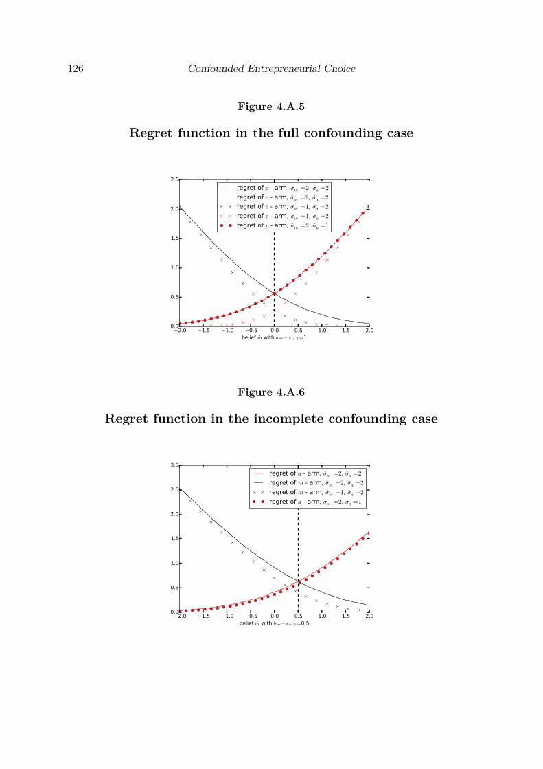
126 Confounded Entrepreneurial Choice
Figure 4.A.5
Regret function in the full confounding case
2.0 1.5 1.0 0.5 0.0 0.5 1.0 1.5 2.0belief m with b=−∞, γ=1
0.0
0.5
1.0
1.5
2.0
2.5
regret of p - arm, σm =2, σa =2
regret of e - arm, σm =2, σa =2
regret of e - arm, σm =1, σa =2
regret of p - arm, σm =1, σa =2
regret of p - arm, σm =2. σa =1
Figure 4.A.6
Regret function in the incomplete confounding case
2.0 1.5 1.0 0.5 0.0 0.5 1.0 1.5 2.0belief m with b=−∞, γ=0.5
0.0
0.5
1.0
1.5
2.0
2.5
3.0
regret of a - arm, σm =2, σa =2
regret of m - arm, σm =2, σa =2
regret of m - arm, σm =1, σa =2
regret of a - arm, σm =2. σa =1

Plots and Tables 127
Figure 4.A.7
Informational benefits after the first period, homogeneousinitial uncertainty and noise
0.0 0.2 0.4 0.6 0.8 1.0Correlation coefficient, ρ
0.50
0.55
0.60
0.65
0.70
0.75
0.80
Unce
rtain
ty r
educt
ion σ
2 z,1
σ2 z,0
p-arm in the first periode-arm in the first period
0.0 0.2 0.4 0.6 0.8 1.0Scaling of ability, γ
0.60
0.65
0.70
0.75
0.80
0.85
0.90
0.95
1.00
Unce
rtain
ty r
educt
ion σ
2 z,1
σ2 z,0
Figure 4.A.8
Informational benefits after the second period, homogeneousinitial uncertainty and noise
0.0 0.2 0.4 0.6 0.8 1.0Correlation coefficient, ρ
0.3
0.4
0.5
0.6
0.7
0.8
0.9
1.0
Unce
rtain
ty r
educt
ion σ
2 z,2
σ2 z,0
p-arm twicee-arm twiceeach arm once
0.0 0.2 0.4 0.6 0.8 1.0Scaling of ability, γ
0.3
0.4
0.5
0.6
0.7
0.8
0.9
1.0
Unce
rtain
ty r
educt
ion σ
2 z,2
σ2 z,0

128 Confounded Entrepreneurial Choice
Figure 4.A.9
Informational benefits after the first period, heterogeneousinitial uncertainty and noise
0.0 0.2 0.4 0.6 0.8 1.0Correlation coefficient, ρ
0.50
0.55
0.60
0.65
0.70
0.75
0.80
0.85
Unce
rtain
ty r
educt
ion σ
2 z,1
σ2 z,0
p-arm in the first periode-arm in the first period
0.0 0.2 0.4 0.6 0.8 1.0Scaling of ability, γ
0.60
0.65
0.70
0.75
0.80
0.85
0.90
0.95
1.00
Unce
rtain
ty r
educt
ion σ
2 z,1
σ2 z,0
Figure 4.A.10
Informational benefits after the second period, heterogeneousinitial uncertainty and noise
0.0 0.2 0.4 0.6 0.8 1.0Correlation coefficient, ρ
0.0
0.2
0.4
0.6
0.8
1.0
Unce
rtain
ty r
educt
ion σ
2 z,2
σ2 z,0
0.0 0.2 0.4 0.6 0.8 1.0Scaling of ability, γ
0.0
0.2
0.4
0.6
0.8
1.0
Unce
rtain
ty r
educt
ion σ
2 z,2
σ2 z,0
p-arm twicee-arm twiceeach arm once

Proofs 129
Figure 4.A.11
Illustration of reservation thresholds as a function of ρ and γ
−0.6 −0.4 −0.2 0.0 0.2 0.4 0.6
Individual belief zt = mt − (1− γ)at
γ = 1, ρ = 0
γ = 0, ρ = 0.8
z0
zp1
ze1
z2, identical in both cases
zp1 ze
1
z0
bad entrepreneurs good entrepreneurs
Figure 4.A.12
Frictionless assignment
−4 −3 −2 −1 0 1 2 3 4
General ability a∗
−4
−3
−2
−1
0
1
2
3
Bus
ines
sac
umen
m∗
light gray area:entrepreneurship is optimal
dark gray area:non-participation is optimal
white area:payroll job is optimal
0.0400.
080
0.120
0.160
0.20
0
0.240
Allocation of individuals to activities in the absence of information friction
SMM results and effects of confounding and non-participation
Non-pecuniary benefits
4.B: Proofs
In this section the proofs for analytical results are provided.

130 Confounded Entrepreneurial Choice
Figure 4.A.13
Initial Beliefs
−4 −3 −2 −1 0 1 2 3 4
General ability a∗
−5
−4
−3
−2
−1
0
1
2
3
Bus
ines
sac
umen
m∗
R1, e > p > n
R5, n > e > p
R6, e > n > p
R2, p > e > n
R3, p > n > eR4, n > p > e
0.015
0.03
0
0.045
0.0600.
0750.090
0.10
5
Distribution of initial beliefs
Table 4.A.1
Estimated Parameters
Estimated parameters of the baseline model. The variance of initial estimates σ2a,0, σ2
m,0 are asum of population uncertainty σ2
a∗ , σ2m∗ and the variance of initial signals σεa,0 = 0.81, σεm,0 =
1.05. Value of initial uncertaint on ability pinned down by an exogenous requirement of fullidentification of a∗ at the end of the learning period.
Parameter estimatemean population ability µa∗ 0(norm.)mean population acumen µm∗ -1.68std population ability σa∗ 0.64std population acumen σm∗ 0.91scaling of ability in entrepreneurship γ 0.85initial uncertainty about ability σa,0 1.02initial uncertainty about acumen σm,0 1.39std of individual shocks in entr. σe 0.87std of individual shocks in emp. σp 0.51value of home production b -0.72
Proof of Proposition 1 and 2. Let the data be yt =(yp
1, ..., yptp
, ye1, ..., ye
te
). The likelihood

Proofs 131
Table 4.A.2
Targeted moments - model versus non-pecuniary benefitsSMM implied targeted moments based on the main specification of the model estimated pa-rameters - consequences of non-pecuniary benefits in entrepreneurship.
Targeted Moments data model + non-pecuniary
σ(log
(yp
i,t
))0.73 0.71 0.74
σ(log (yp
i ))
0.60 0.59 0.63σ(log
(ye
i,t
))1.08 1.07 1.13
σ(log (ye
i ))
0.83 0.86 0.84corr
(log
(yp
i,t
), log
(ye
i,t
))0.68 0.65 0.60
ratio of mean incomes entr.emp. 1.02 1.04 0.97
non-participation rate 0.10 0.08 0.06cross-sec. entrepreneurship rate 0.06 0.10 0.20
Table 4.A.3
Untargeted moments - model versus non-pecuniary benefitsSMM implied untargeted moments based on the main specification of the model estimatedparameters - consequences of non-pecuniary benefits in entrepreneurship.
Untargeted Moments data model + non-pecuniaryratio of medians entr.
emp.0.84 0.93 0.84(target)
frac. of underpeforming entr. 0.36 0.25 0.47share of serial entrepreneurs 0.39 0.51 0.36ever trying entrepreneurship 0.29 0.71 0.92share of 1-2 p. spells in entr. 0.68 0.54 0.22share of entries with 0-5 experience 0.41 0.65 0.77entr. rate up to 5 yrs. of activity 0.03 0.45 0.53
of the data can be written as:
L(yt|a∗, m∗) ∝ exp
{−
(1
2σ2e
te∑j=1
(ye
j − a∗ − m∗)2 + 12σ2
p
tp∑j=1
(yp
j − a∗)2
)}=
exp
{−te
2σ2e
(1te
te∑j=1
(yei )2 − 2 (a∗ + m∗) ye + (a∗ + m∗)2
)−te
2σ2e
(1te
te∑j=1
(yei )2 − 2 (a∗) ye + (a∗)2
)}.
So that ye is a sufficient statistic for a∗ + m∗ with variance σ2e
teand yp is a sufficient

132 Confounded Entrepreneurial Choice
Table 4.A.4
Cost of information frictionRelative productivity change ∆ in response to reduction of initial uncertainty measured as aratio of median incomes before and after the change in prior uncertainty and the accompanyingratio of median incomes in the two types of employment.
∆ entr ∆ emp. median entr.emp.
decrease in σ2a,0 by 10% 1.011 1.000 0.95
decrease in σ2a,0 by 50% 1.048 1.006 0.99
decrease in σ2a,0 by 100% 1.207 1.011 1.14
decrease in σ2m,0 by 10% 1.033 1.005 0.96
decrease in σ2m,0 by 50% 1.106 1.010 1.05
decrease in σ2m,0 by 100% 1.238 1.016 1.16
statistic for a∗ with variance σ2p
tpwhich proves Corollary 1. Observe that the difference
ye − yp is a sufficient statistic for m∗. Corollary 2 follows as the value of home production
is independent of It.
The ommission of γ is without loss of generality, as an alternative is to formulate
the model with ability gains 1γ, 0 < γ ≤ 1 in payroll employment as follows:
yp = 1γ
a∗ + εp
ye = a∗ + m∗ + εe
so that it’s possible to introduce a new signal yp = γyp with variance σ2p = γ2σ2
p.
Proof of Theorem 1. Let’s assume that the prior on (a∗, m∗) is a bivariate normal with
mean vector µ and variance-covariance matrix Σ as follows:
µ =
a0
m0
Σ =
σ2a,0 ρσa,0σm,0
ρσa,0σm,0 σ2m,0
.

Proofs 133
Then, the posterior H(a∗, m∗|y =
{ye
1, yete
, yp1, ..., yp
tp
})is:
H ∝ exp −
1
2σ2e
te∑j=1
(ye
j − γa∗ − m∗)2
+ 12σ2
p
tp∑j=1
(yp
j − a∗)2+
11 − ρ2
((a∗ − a0)2
σ2a,0
+ (m∗ − m0)2
σ2m,0
− 2ρ (a∗ − a0) (m∗ − m0)σa,0σm,0
).
The posterior can be collapsed to the following representation:
H ∝ exp −12
(a∗)2(
γ2te
σ2e
+ tp
σ2p
+ 1(1 − ρ2
0) σ2a,0
)+ (m∗)2
(te
σ2e
+ 1(1 − ρ2
0) σ2m,0
)
+ a∗(
γteye
σ2e
+ tpyp
σ2p
+ a0
(1 − ρ20) σ2
a,0− ρ0m0
(1 − ρ20) σa,0σm,0
)
+ m∗(
teye
σ2e
+ m0
(1 − ρ20) σ2
m,0− ρ0a0
(1 − ρ20) σa,0σm,0
)
+ a∗m∗(
ρ0
(1 − ρ20) σa,0σm,0
− γte
σ2e
)
Lemma 4.1 (Parametrization of the posterior). The distribution of (x, y) on the plane
that is proportional to
exp −12[ax2 − 2bx + cy2 − 2dy − 2exy
]is a bivariate normal with means µx, µy:
µx = bc + ed
ac − e2 µy = da + eb
ac − e2 ,
variances σ2x, σ2
y:
σ2x = c
ac − e2 σ2y = a
ac − e2 ,
and correlation ρ:
ρ = e√ac
The proof follows from algebraic expansion of the distribution formula and can be
found in Farzinnia and McCardle (2010)]. By applying this approach we can identify

134 Confounded Entrepreneurial Choice
the posterior parameters as a, b, c, d, e naturally follow5:
a = γ2te
σ2e
+ tp
σ2p
+ 1(1 − ρ2
0) σ2a,0
b = γteye
σ2e
+ tpyp
σ2p
+ a0
(1 − ρ20) σ2
a,0− ρ0m0
(1 − ρ20) σa,0σm,0
c = te
σ2e
+ 1(1 − ρ2
0) σ2m,0
d = teye
σ2e
+ m0
(1 − ρ20) σ2
m,0− ρ0a0
(1 − ρ20) σa,0σm,0
e = ρ0
(1 − ρ20) σa,0σm,0
− γte
σ2e
.
What is left is to plug these results back to Lemma 4.1 equations.
Martingale property of beliefs. The proof involves tedious and cumbersome algebraic
manipulations. Mathematica codes deriving the martingale property of beliefs are avail-
able on request from the author.
Regret Properties. First, let’s show that the regret is increasing in uncertainty. To do
that let’s consider within-period regret. It has the following form:
∂R (It, ξ)∂σm,t
= ϕ
(− mt
σm,t
)1 +(
mt
σm,t
)2
+ mt
σm,t
> 0 ∀mt, σm,t
Observe that when m > 0 all the factors of the sum in the square bracket are
positive. When −1 < mσm,t
< 0 the last two factors are jointly negative but less than 1
in absolute value and the sum remains positive. Finally, when mσm,t
< −1 the squared
term dominates the last negative factor and the sum again is positive. For the case of
0 < γ < 1, let’s introduce a variable z∗ = m∗ + (γ − 1) a∗ and then the regret can be
rewritten as:
Et [y (ξ∗) − y (ξt) |It] =
(1 − ΦIt
(− zt
σz,t
))zt + σz,tϕ
(− zt
σz,t
)if ξt = p
−Φ(− zt
σz,t
)zt + σz,tϕ
(− zt
σz,t
)if ξt = s.
5Observe that the formula for the e-term in (Farzinnia and McCardle, 2010) contains an error.

Numerical algorithm 135
4.C: Numerical algorithm
The problem of each agent is uniquely identified by initial beliefs m0, a0, t = te + tp
and ye, yp. At step t the belief distribution is given accordingly to the Theorem 1 in the
paper. The algorithm proceeds as follows:
1. Given the distribution F (a, m) construct a grid of pairs (ai, mj)i,j∈{1,...,Ng} that
approximates F .
2. For each initial belief means (ai, mj) construct a grid on sufficient statistics space
(ye (i, j)k , yp (i, j)l)i,j∈{1,...,Nm} × (te, tp). The set of productive times (te, tp) has
the power equal to the number of integer solutions to the diophantine equation
t = te + tp which equals(
t+22
).
3. Solve the P problem by backward induction, approximating the within-period
regret with a product Gauss-Hermite quadrature and using two-dimensional linear
interpolation for the next period value function to obtain the switching thresholds
for each sufficient statistic. Observe that choosing ξt = ξn implies ξn is chosen for
all future periods.
4. Simulate Na agents indexed by k with initial belief (ai, mj) and true endowment
(a∗k, m∗
k), interpolating the switching thresholds implied by the solution to P .
5. Store the status in employment for each agent k in time t and the earnings yk,t
weighted by the probability mass at (ai, mj), discard the value function and policy
functions, move to the next (a, m) pair.
The main advantage of the last two steps is that they save on backward induction
step which is the most costly part of the algorithm. It does introduce, however, some
inaccuracy in the first period as all Na (i, j) agents make identical first period choice,
their trajectories begin to differ with the first period different income realisations. The
SMM exercise target function is a weighted sum of squared deviations from the targeted

136 Confounded Entrepreneurial Choice
moments. The key source of possible inaccuracy is the location of first period switching
threshold in the z space and the rate at which it goes to zt = 0 boundary. Thus, I use
a finer grid for the approximation of F at the expense of the grid on average returns.
The policy functions tend to differ only near the switching thresholds, thus the policy on
sufficient statistics which are off the grid are usually well approximated by the policy at
the boundary. The grid on average returns is chosen endogenously, conditionally on the
initial belief means and uncertainty. Observe that the number of agents Na has virtually
no bearing on the computational cost, as it relies on the same value function at a given
(ai, mj) pair which is collapsed to two reservation thresholds at any of the histories te, tp.
Thus, I have Ng = 20, Nm = 15, Na = 500.

Chapter 5
Efficient insurance in market theory of
payroll and self-employment
5.1. Introduction
Over the last two decades, the majority of the developed economies have experienced
a shift in the composition of employment towards more own-account work and freelanc-
ing. For example, about half of the new jobs taken up in the United Kingdom in the
last decade were self-employment jobs. As a result of the shift in the composition of
employment, the self-employed now constitute a group larger than the unemployed in
many countries. Furthermore, there is significant variation of the self-employment rate
between developed economies. These facts, illustrated in Table 5.1, are difficult to rec-
oncile with existing theories of self-employment that emphasize individual heterogeneity
of skills, preferences, or cognitive biases (Parker, 2012), which we don’t expect to vary
much over time and across countries.
To make this point more rigorously and go beyond anecdotal evidence, we com-
piled a sample of 19 OECD countries for years 1990-2009 and regressed the log of self-
employment rate on logs of unemployment rate, benefit-wage replacement rate and the
level of GDP (all lagged) and a time trend. Table 5.2 provides an overview of what we
treat as unconditional correlations in the data. This simple exercise confirms the widely

138 Market theory of payroll and self-employment
Table 5.1
Incidence of own-account workShare of own-account workers in total employment. Source: Key Indicators of the LaborMarket, ILO.
Country 1993 2013
UK 9.1 11.7Netherlands 6.9 11.8Germany 4.0 6.0Italy 11.8 16.4Sweden 7.8 6.4Denmark 4.7 5.4
held belief that the self-employment rate decreases in the level of GDP per capita, de-
creases in the generosity of UI for employees but there also is a significant time trend.
Although it’s impossible to claim causality in this exercise, we believe that the coeffi-
cients of this regressions provide a proxy of unconditional correlations in the data and
further corroborate our narrative.
In this paper we propose a theory of the composition of employment that focuses on
the key distinction between self- and payroll employment: exposure to the risk of not
selling output versus exposure to the risk of not finding a job. The self-employed are the
sole claimants of the fruits of their labor, but bear the risk of not selling their products
or services fully on their own. The wage contract limits this risk for the employee, but
requires sharing any surplus of a match with the firm. Moreover, not all of those looking
for a wage contract are able to find one, so that some become unemployed. In order
to highlight these differences between payroll and self-employment, we explicitly and
jointly model the problems of finding a job in the labor market and selling output in the
goods market.
All developed countries offer some form of unemployment insurance for those that
do not find a job. Denmark and Sweden have recently also introduced unemployment

Introduction 139
Table 5.2
Pooled OLS estimationEvidence for 19 OECD countries for the years 1990-2009. Log of replacement rate of wageswith benefits b
w for married households, u is the log of unemployment rate and YN is the log
of GDP per capita, SE is the log of the self-employment rate, time is the linear time trendvariable.
explained variable: SEt
ut−1 -0.0334(0.0468)
YN t−1 -1.172***
(0.0991)bw t−1 -0.286***
(0.110)time 0.0177***
(0.00402)N 321R2 0.417Standard errors in parentheses* p < 0.1, ** p < 0.05, *** p < 0.01
insurance schemes that are designed specifically for the self-employed. However, in the
majority of developed countries this type of insurance is still absent. On the one hand,
it is widely believed that being self-employed is riskier than being an employee. On the
other hand, if self-employment is driven by the desire to be one’s own boss or by higher
tolerance for risks, insurance for the self-employed is hard to justify.
We aim to make two contributions. First, we propose a novel parsimonious theory
of self-employment that does not rely on individual-level differences between people but
focuses on trade-offs between labor and goods market frictions. Changes in these mar-
kets, possibly resulting from the spread of modern communication technologies, provide
a natural explanation for the long run behavior of self-employment rates.
Second, we show that there should be insurance benefits for the self-employed that fail
to sell, solely for the purpose of maximizing the volume of goods traded with customers.
Insurance for the self-employed eliminates business stealing by risk averse self-employed

140 Market theory of payroll and self-employment
who have an incentive to set their prices too low from the societal point of view, in order
to reduce the risk of not selling their output. This paper therefore provides a rationale
for the UI policies of Denmark and Sweden that is not only based on risk sharing, but
also on efficiency.
We consider an economy represented in Figure 5.1. It is inhabited by homogenous
individuals producing an indivisible good. The good cannot be consumed by these
individuals but can be exchanged with buyers for a divisible endowment from which
the individuals do derive utility. The individuals face a one-shot career choice problem.
They can either become self-employed, which implies producing and trying to sell their
output by themselves, or seek a job at a firm, which tries to sell the goods produced by
the individual it employs.
Individuals entering the labor market cannot coordinate their job applications to
firms that post wages, which results in involuntary unemployment. Similarly, buyers
cannot coordinate their visits to firms and self-employed that post prices, resulting in
unsold inventories. An employee is guaranteed the wage even if the firm fails to sell
the goods. However, an employee has to share the expected surplus with the firm. The
self-employed face the risk of not selling, but they forego the risk of unemployment.
Unlike in the standard Mortensen-Pissarides framework, in our model a match with a
firm is thus not necessary to generate income. Our model endogenously determines a
vacancy and self-employment rate depending on, among others, search technology and
the existence of some advantageous business conditions for firms. One can think of these
advantageous business conditions as productivity or quality gains to firm formation,
resulting from additional capital, training or knowledge that the firm has at its disposal
after the investment of an entry cost k. In a richer framework with intermediate inputs,
such gains may result from economizing on internal transaction costs as in Coase (1937).
Alternatively, advantageous business conditions for firms can result from a superior
visibility in the goods market after the investment of cost k. This is the interpretation
used in this chapter. Firms in our model are both an intermediary between the employee

Introduction 141
Figure 5.1
A snapshot of the model economy
Individualsindivisible endowment (leisure)
want buyers’ endowmentcan produce indivisible goodscannot consume these goods
Firmsshares traded in fin. marketmaximize expected profitsneed worker to producepost one vacancy, cost k
Buyersdivisible endowment (money)
want one indivisible goodvalue of buying vb = 1
value of not buying = 0
competitive search
competitive search
and the buyers, and a vehicle of production and marketing that cannot exist without any
form of competitive advantage over independent production by the self-employed. Yet,
the trade-off between the frictions in the goods and labor market leads to the coexistence
of firm employment and self-employment in equilibrium.
The presence of firms and self-employed implies the goods market consists of two
different types of sellers. If individuals are risk averse, these two different types of
sellers have different objectives, creating inefficiencies that can be potentially corrected
by policy. Risk averse self-employed, unlike risk neutral firms, have an incentive to
self-insure via their pricing decision. By decreasing prices they attract on average more
buyers so that their selling probability increases. However, the lowering of prices by
the self-employed steals business away from firms. Other things equal, firms’ expected
profits fall. Consequently, fewer firms enter and the economy benefits to a lesser extent
from their advantageous business conditions. As a result, the volume of the goods traded

142 Market theory of payroll and self-employment
drops.
The ability to self-insure makes a career in self-employment relatively more attractive
than entering the labor market. This effect is countered by the conventional effect
that firms post lower wages to increase the job finding rate of risk averse job seekers.
The latter, however, comes at the cost of excessive vacancy creation. Generally, the
employment composition is different than the composition that would maximize the
volume of goods traded net of firm entry costs. For some parameter values, the ability
to self-insure in self-employment can dominate the market insurance offered by firms.
As a result, the self-employment rate may increase in risk aversion.
We find that the combination of type-of-employment dependent lump-sum taxes and
income support benefits under a balanced budget can maximize the output sold net of
entry costs, while offering insurance to risk averse individuals. This optimal policy mix
consists of differentiated taxes and unemployment insurance benefits for both workers
and self-employed. Optimal UI benefits for the self-employed eliminate business stealing,
while optimal UI benefits for job seekers raise wages and stop excessive firm entry.
Differentiated taxes then balance the budget while ensuring an optimal employment
allocation via the career choice of individuals. We show that whenever the job finding
probability exceeds the selling probability (so that the self-employment income can be
considered riskier), the UI benefits for the self-employed should be more generous than
the UI benefits for employees.
Related literature. Our paper is related to three strands of the literature: on the
drivers of self-employment, on frictional goods markets and intermediation, and on op-
timal unemployment insurance. Below we describe our contribution to those papers.
There is a variety of theories explaining self-selection into self-employment. A large
fraction of this literature puts individual characteristics and heterogeneity as a reason
for self-employment. We list a limited selection of those papers, whereas Parker (2004)
offers an extensive survey. Lucas (1978), Jovanovic (1982) and Poschke (2013) assume

Introduction 143
that being an entrepreneur/self-employed requires a separate skill, potentially different
than a skill needed to be an employee. Kihlstrom and Laffont (1979) postulate differ-
ences in risk aversion that lead to undertaking entrepreneurial activities. De Meza and
Southey (1996) find that self-employed entrepreneurs are significantly more optimistic
than employees. Lindquist et al. (2015) document the importance of family background.
We complement this literature, because in our model self-employment is an equilibrium
outcome that does not require any ex ante individual heterogeneity. Besides, Rissman
(2003, 2007) assumes returns to self-employment are drawn from an exogenous distribu-
tion riskier than the wage distribution. We offer a model that endogenously generates
those risk differentials. Finally, our model is complementary to papers that explain self-
employment from financing frictions (Evans and Jovanovic, 1989; Buera, 2009), because
a frictional financial market could be introduced as an additional stage in the career
choice game for those who choose self-employment.
To the best of our knowledge, self-employment has not been introduced into models
with frictions in the goods market. Existing papers study the macroeconomic conse-
quences of goods market frictions (See e.g. Michaillat and Saez (2015); Petrosky-Nadeau
and Wasmer (2015); Kaplan and Menzio (2013)), or characteristics of firms that operate
in a frictional goods market. Most closely related are Shi (2002), who explains the size-
wage differential in the labor market by a sufficiently large size-revenue differential in the
goods market, and Godenhielm and Kultti (2009), who allow for endogenous capacity
choice and study the resulting firm size distribution.
Our model can also be framed as a choice of producers to trade with buyers via
a middleman (firm) or to trade with buyers directly. The papers in the literature on
intermediation that are most closely related are Watanabe (2010, 2013). Unlike in those
papers, the choice that producers (individuals) face in our model is exclusive. Also, the
meetings with the middlemen are subject to a friction. Wright and Wong (2014) offer a
general model of middlemen with search and bargaining problems. We employ posting,
allow for bypassing of the middlemen, and discuss labor policy implications.

144 Market theory of payroll and self-employment
Papers on efficient unemployment insurance for risk averse individuals either do
not take self-employment (e.g. Acemoglu and Shimer (1999)) or market frictions into
account (e.g. Parker (1999)). Our paper shows that the interaction of risk averse self-
employed and goods market frictions is crucial for understanding efficient unemployment
insurance.
The rest of the paper is organized as follows. In Section 5.2 we outline the structure
of the model. Then, in Section 5.3 we characterize the market equilibrium. In Section
5.4 we present and characterize the conditions under which a unique mixed strategy
equilibrium exists, and prove that it maximizes net output sold for risk neutral pref-
erences. In Section 5.5 we show that the decentralized allocation is not efficient for
risk averse preferences, but that introducing a type-of-employment dependent tax and
unemployment insurance policy can restore efficiency. Section 5.6 presents the steady
state of a dynamic version of the model in which jobs in expectation last for multiple
periods, and shows how the composition of employment depends on the key parameters
of the model. The final section concludes.
5.2. Model environment
We consider a one-shot game of an economy populated by firms, buyers, and individu-
als interacting in two markets. Individuals face a career choice between self-employment
and entering the labor market. In the goods market, firms and the self-employed ex-
change with buyers an indivisible produced consumption good (a coconut) for a divisible
endowment (money). In the labor market, individuals exchange with firms indivisible
labor for money. There are coordination frictions in both markets.
Population and technology. The measure of individuals is normalized to one. In-
dividuals value consumption according to a weakly concave utility function u (c), suffer
no disutility from labor, but cannot consume coconuts. Instead, they derive utility from

Model environment 145
money.1 For convenience, we also postulate that u (0) = 0. There is a unit mass of buyers
B in the goods market that can consume money and exactly one coconut. They enjoy a
utility v from consuming the coconut, and a smaller, linear utility from their endowment
of money, which individuals can also consume. We normalize buyers’ utility from not
buying to zero and the utility from consuming the coconut to one. We consider a partial
equilibrium setup with buyers and individuals living in separate households. Finally,
there is an endogenously determined mass V of vacancies opened by profit-maximizing
firms upon paying a cost k > 0.
The career choice of individuals results in an endogenous measure SE of self-employed
and LM = 1 − SE of agents entering the labor market. A match of a single worker
and vacancy results in an active firm. The measure of active firms is denoted by F .
Because of search frictions in the labor market we have F ≤ V . Both a self-employed
and an active firm produce one coconut. Each opens one outlet to sell its coconut in the
goods market and posts a price with commitment. However, an active firm’s outlet and
price is visible in the goods market with probability A ∈ (0, 1], whereas a self-employed
individual’s outlet and price is visible with probability a ∈ (0, 1].2 One can also think of
1 − A and 1 − a as probabilities of a coconut rotting before the goods market opens up.
Goods Market. Buyers observe prices of visible outlets, can only visit one of these,
but cannot coordinate which one to visit. For that reason, the goods market is subject
to urn-ball frictions. As a result, some visible sellers face more customers than they can
serve and others are not able to sell, while some buyers fail to buy the good. If there is a
mass of buyers BSE at the visible outlets opened by the self-employed, then the average
queue length at each outlet is xSE = BSE/(aSE). The average queue length of buyers at
1For instance, because money can be exchanged in a perfectly competitive third market for anotherdivisible consumption good (which is thus not a coconut).
2Here we allow for differences in the visibility of self-employed and active firms. This formulation isnot restrictive. A model in which a and A denote the number of coconuts produced by the self-employedand active firms, respectively, is almost identical (exactly identical under risk neutral preferences) aslong as every coconut is sold in a separate outlet. If multiple coconuts are sold at one outlet, thereexists a selling advantage to larger inventories, see Watanabe (2010). Alternatively, one can write avery similar model with differences in qualities of coconuts, which scale up the utility of buyers.

146 Market theory of payroll and self-employment
a visible active firm xF is defined analogously. The corresponding service probabilities for
a buyer are denoted by η (xSE) and η (xF ), at self-employed and active firms respectively.
The selling probabilities of visible outlets λ (xSE) = xSEη (xSE) and λ (xF ) = xF η (xF )
are the complementary probabilities of having no buyers visiting a visible outlet at all.
Using the large market assumption to characterize these probabilities, λ (x) = 1 − e−x.
Labor Market. Upon paying an entry cost to open a vacancy, a firm posts a wage
and commits to it. Workers observe all wages but can apply to one vacancy only, while
a vacancy can be filled by only one worker. As standard in the literature, to capture the
coordination frictions we restrict our attention to symmetric and anonymous strategies.
We denote the average queue length by xLM = LM/V where V is the measure of open
vacancies. Due to coordination frictions, some firms fail to fill their vacancy and do
not become active, while some workers remain unemployed. The probability of filling a
vacancy is denoted by q (xLM), and by the large market assumption q (xLM) = 1−e−xLM .
The job finding probability is simply µ (xLM) = q (xLM) /xLM . Finally, we assume that
the firms can insure in a competitive market against the risk of not being able to pay
the wage, so that the worker is guaranteed a wage once matched. The shares of firms are
traded by financial investors (not modeled explicitly) who can buy a market portfolio of
those shares so that the firms maximize expected profits upon entry.
Timing. The timing of the game is displayed in Figure 5.2. First, a measure of firms
enter the labor market by opening vacancies. In the career choice stage the unit mass
of individuals parts into self-employed and prospective workers. In the third stage, the
frictional labor market matches vacancies and prospective workers, resulting in a measure
F = q (xLM) V of active firms and a measure U = (1 − µ (xLM)) LM of unemployed
workers. In the fourth stage, all active firms and self-employed individuals produce and
become sellers in the goods market. In the fifth stage, a fraction of the sellers become
visible and buyers direct their search to them such that the following accounting identity
is satisfied:
axSESE + AxF F = 1, (5.1)

Equilibrium definition 147
Figure 5.2
Timing of events
-t = 0 t = 1
?
firmsenter
?
careerchoice
?
labormarket
?
production
?
goodsmarket
?
individualsconsume
which means that no buyers stay at home not trying to visit any seller. Now we are in
position to define the market equilibrium of this economy in the following section.
5.3. Equilibrium definition
We decompose the one-shot game into two stages: the career choice and the labor
market as the first stage, and the goods market as the second stage. We solve the game
backwards, starting from the goods market. We focus on equilibria that feature both
self-employment and payroll employment. The existence conditions for such a mixed
strategy equilibrium of the career choice game are presented in the next section.
Goods market. As is standard in competitive search models, separate submarkets
open and buyers choose between visiting each of the submarkets such that in equilibrium
they are indifferent between all active submarkets and obtain value V B. Given the
specification of buyers preferences, this value reads
V B = η (xF ) (1 − pF ) = η (xSE) (1 − pSE) . (5.1)
Given that the wage is sunk, active firms maximize expected revenue: Aλ (xF ) pF .
The self-employed maximize expected utility. The expected value of self-employed sell-
ers, dropping zero utility of not receiving any income, is then
V SE = aλ (xSE) u (pSE) . (5.2)
The goods market outcomes and payoffs are depicted in Figure 5.3.

148 Market theory of payroll and self-employment
Figure 5.3
Goods market sub-equilibrium
Self-Employed, SE Active Firms, F
SE submarketprice pSE
queue length:xSE = BSE
aSEselling probability:
aλ (xSE) = a (1 − exp (−xSE))buying probability:η (xSE) = λ(xSE)
xSE
F submarketprice pF
queue length:xF = BF
AFselling probability:
Aλ (xF ) = A (1 − exp (−xF ))buying probability:
η (xF ) = λ(xF )xF
Buyers, B1 = BF + BSE
Equilibrium: V BSE = V B
F
V SE = aλ (xSE) pSE revenue = Aλ (xF ) pF
V BF = η (xF ) (1 − pF )V B
SE = η (xSE) (1 − pSE)
Sellers post prices to maximize their expected payoffs subject to the constraint that
buyers must receive their market utility V B. The optimal prices and an associated goods
market sub-equilibrium characterization are presented below.
Lemma 5.1 (Optimal price posting). Assume SE > 0, F > 0, BF > 0, BSE > 0 fixed.
Let ϕ (x) = −x∂η(x)η(x)∂x
be the elasticity of the buying probability with respect to the queue
length x. Given queue lengths xSE = BSE
aSE, xF = BF
AFthe optimal price posting conditions
are:
ϕ (xSE) (1 − pSE)1 − ϕ (xSE)
= u (pSE)u′ (pSE)
, (5.3)
pF = ϕ (xF ) . (5.4)
Proof. See Appendix 5.A.

Equilibrium definition 149
Definition 5.1 (Goods market sub-equilibrium). Let SE > 0, F > 0 be fixed. A goods
market sub-equilibrium is a tuple {xSE, xF , pSE, pF } such that given xSE, xF the sellers
optimally post prices according to (5.3) and (5.4), and the buyers’ indifference condition
(5.1) and accounting identity (5.1) hold.
Labor market. Now we consider a non-zero mass of prospective workers LM > 0 and
analyze labor market outcomes. We do that in two steps. First, we fix the measure of
vacancies V > 0; then we allow for free entry in posting vacancies by prospective firms.
Given that the entry cost k is sunk, potential firms post a wage in the labor market
to maximize expected profits, taking into account equilibrium outcomes in the goods
market. They compete with other potential firms for workers, under the constraint that
they must at least offer the market utility level of workers searching for jobs:
V LM = µ (xLM) u (w) . (5.5)
Lemma 5.2 (Optimal wage posting). Assume LM > 0 and V > 0 fixed. Given queue
length xLM = LM/V , the optimal wage w that maximizes firms profits subject to workers’
market utility (5.5) solves the following equation:
ϕ (xLM) [Aλ (xF ) pF − w]1 − ϕ (xLM)
= u (w)u′ (w)
, (5.6)
where pF and xF come from the goods market sub-equilibrium {xSE, xF , pSE, pF } induced
by SE = 1 − LM and F = q (xLM) V and where ϕ (xLM) = xLM ∂q(xLM )q(xLM )∂xLM
is the elasticity
of the job filling probability with respect to the queue length.
Proof. See Appendix 5.A.
Expected profits are therefore shared with workers according to the elasticity of the
matching function in the labor market, and are decreasing in risk aversion. By posting
lower wages when workers are risk averse, firms offer market insurance in the form of
higher job finding probabilities from larger firm entry. The free-entry condition drives
the value of posting a vacancy net of the entry cost k down to zero. Firms’ entry takes

150 Market theory of payroll and self-employment
Figure 5.4
Labour market sub-equilibrium
Prospective Workers, LM Vacancies, V
Labor Marketwage w
queue length:xLM = LM
Vjob filling probability:
q (xLM ) = 1 − exp (−xLM )job finding probability:
µ (xLM ) = q(xLM )xLM
Unemployed, UU = (1 − µ (xLM )) LM
Active Firms, FF = q (xLM ) V
V LM = µ (xLM ) u (w)
entry cost k
expected revenuesq (xLM ) (AλF pF − w)
into account the resulting goods-market sub-equilibrium where SE = 1−LM . Formally,
we can define the labor market sub-equilibrium as follows.
Definition 5.2 (Labor market sub-equilibrium). Assume LM, SE > 0. The labor mar-
ket sub-equilibrium is a pair {xLM , w} such that given xLM , firms optimally post wages
according to (5.6) and the following free-entry condition holds:
q (xLM) [Aλ(xF )pF − w] − k = 0, (5.7)
with pF and xF from the goods market sub-equilibrium {xSE, xF , pSE, pF } induced by SE
and F = q (xLM) V with V = LM/xLM .
The labor market equilibrium is represented in Figure 5.4. Now we are in the position
to define a mixed strategy equilibrium for our career choice game.
Definition 5.3 (Mixed strategy career choice equilibrium). A mixed strategy career
choice equilibrium is a tuple {SE∗ > 0, LM∗ > 0, x∗LM , w∗, x∗
SE, x∗F , p∗
F , p∗SE} such that:

Equilibrium definition 151
1. all individuals either become self-employed or enter the labor market: SE∗+LM∗ =
1;
2. given SE∗ and LM∗, {x∗LM , w∗} is a labor market sub-equilibrium,
and {x∗SE, x∗
F , p∗SE, p∗
F } is a corresponding goods market sub-equilibrium;
3. individuals are indifferent between self-employment and entering the labor market,
i.e. V SE∗ = V LM∗ as defined in (5.2) and (5.5), respectively.
Observe that the indifference condition requires that whenever the job finding prob-
ability µ exceeds the selling probability λ the income from self-employment is higher,
conditional on selling, than the wage (and the opposite holds when λ > µ).
An interesting special case of the mixed strategy equilibrium is the case of risk neu-
tral individuals. If the self-employed are risk neutral, they maximize expected revenue
aλ (xSE) pSE. As follows from Lemma 5.1, risk neutral self-employed post prices accord-
ing to pSE = ϕ (xSE). Substituting this price in the buyers’ indifference condition (5.1),
it follows that firm and self-employed sellers can expect the same queue length and set
the same prices.
If workers are risk neutral, the wage posting decision of firms as given in (5.6) implies
w = ϕ (xLM) Aλ (xF ) pF . Substituting this wage in (5.7) results in the following free
entry condition:
q (xLM) [1 − ϕ (xLM)] Aλ(xF )pF = k. (5.8)
Besides, as µ (xLM) ϕ (xLM) = q′ (xLM), the value of being a worker can in this case be
written as
V LM = q′ (xLM) Aλ (xF ) pF . (5.9)
As a result, indifference in the career choice game simply requires
V SE = aλ (xSE) pSE = q′ (xLM) Aλ (xF ) pF = V LM . (5.10)
Because self-employed and firms post the same prices, indifference in career choice im-
plies
a/A = q′ (xLM) = e−xLM → xLM = log(
A
a
)(5.11)

152 Market theory of payroll and self-employment
Thus, if the mixed strategy equilibrium exists, the queue length of prospective workers
is independent of the vacancy posting cost k and only depends on a and A. The next
section shows that the mixed strategy equilibrium can exist, both for risk neutral and
for risk averse preferences.
5.4. Existence and efficiency of equilibrium
In this section we state the conditions and explain the reasons for the existence of a
mixed strategy equilibrium. Afterwards, we prove that it maximizes net output sold if
and only if individuals are risk neutral.
Existence. The equilibrium can be shown to exist, to be unique, and to involve mixing
of careers if the exogenous parameters {a, A, k} are appropriately chosen. Outside of a
certain set of {a, A, k} the equilibrium still exists and is unique but features no mixing
of careers. The proof is an application of the Implicit Function Theorem.
As a first step, using the accounting identities in the goods and in the labor market,
we arrive at the following mixing condition:
LM = 1 − axSE
AxF µ (xLM) − axSE
, 0 < LM < 1. (5.1)
Then, we need to solve for the queue lengths {xSE, xF , xLM} and corresponding
prices of goods and labor {pSE, pF , w} using the remaining six equilibrium conditions.
A necessary condition for this set of equations to have a solution is that the ratio
u (c) /u′ (c) is increasing in c, which holds for any utility function with u′ (c) > 0 and
u′′ (c) < 0. For analytical convenience we make the proof operational under CRRA
preferences. However, as the previous remark implies, this is without loss of generality.
Proposition 5.1 (Existence of equilibrium). Let A, a ∈ (0, 1] fixed and u (c) = c1−γ
1−γwith
γ ∈ [0, 1]. Then there exist numbers k (A, a, γ), k (A, a, γ) such that the mixed strategy
equilibrium described in Definition 5.3 exists and is unique if and only if the following

Existence and efficiency of equilibrium 153
inequalities hold:
A > a, (5.2)
k (A, a, γ) < k < k (A, a, γ) . (5.3)
Furthermore, if k > k (A, a, γ) then SE∗ = 1 and if k < k (A, a, γ) then SE∗ = 0.
Proof. See Appendix 5.A.
A direct result of the working of the proof under risk neutral preferences is the set
of comparative statics encapsulated in Corollary 5.1. Intuitively, the net gain of setting
up a vacancy can be neither too small, nor too big for agents to play a mixed strategy
in the career choice game.
Corollary 5.1 (Comparative statics). Consider risk neutral individuals and a, A and
k such that the conditions (5.2) and (5.3) hold, and let there be a corresponding mixed
strategy career choice game equilibrium {SE∗, LM∗, x∗LM , w∗, x∗
SE, x∗F , p∗
F , p∗SE}. Then,
the following inequalities hold:
∂SE∗
∂k> 0,
∂k
∂A> 0,
∂k
∂A> 0,
∂k
∂a< 0,
∂k
∂a< 0.
There are two reasons a corner solution in the career choice game could occur. First,
there may be no firms willing to enter, so that there is no chance of finding a job on a
payroll. This may happen, for example, when the vacancy posting cost k is prohibitively
large. Second, the business conditions of firms may be too advantageous to sustain self-
employment as a valid alternative to seeking a payroll job.
Hence, the key driving force of the composition of employment in the model is the
relative size of the probabilities of becoming visible in the goods market, adjusted for
entry costs, which can be loosely described by comparing A/k to a. One can argue that

154 Market theory of payroll and self-employment
the spread of modern communication technologies has contributed to a relative increase
in the visibility of the outlets of the self-employed, a. The theory then predicts a rise in
self-employment rates, roughly in line with the recent increases in self-employment rates
as documented in Table 5.1.
More generally, the ratio between A/k and a captures the improvement in business
conditions on top of producing on one’s own that comes with setting up a firm. Cor-
recting expected utility with binomial probabilities, one can interpret A and a as the
number of units produced by active firms and self-employed, respectively, as long as
each unit is sold at a separate outlet. One can then think of the ratio of A/k over a as
a statistic for substitutability between the “self-employment technology” and “payroll
employment technology”, or the additional returns to innovation from firm formation.
For example, a large-scale production industry like an automotive industry is a sector
with a very high A/k and low a. In contrast, one can expect the difference between A/k
and a to be low in service industries like hairdressing or taxi-driving. A prediction of
the model is therefore that self-employment rates are higher in hair-dressing than in the
automotive industry. Another prediction is that when the share of low capital intensity
services in the economy increases, the share of self-employment goes up as well. Finally,
the model can shed some light on cross-country differentials in economic development
and the composition of employment. In underdeveloped countries the technologies that
are used in firms offer very little gains, or no gains at all, from organizing workers and
capital into a firm. As our model predicts, those countries exhibit high self-employment
rates.
Necessity of goods market frictions It turns out that the presence of goods market
frictions is necessary for the co-existence of the two types of employment, unless a
certain knife-edge equation is jointly satisfied by k, a and A. Formally, we can show the
following:
Proposition 5.2 (Knife-edge condition in the absence of goods market friction). Assume
the measure of buyers is infinite so that the probability of selling produced good equals

Existence and efficiency of equilibrium 155
unity once it is visible in the goods market. Then, the type of employment choice features
mixing if, and only if the following equality holds:
k
A= 1 − a
A
(1 − log
(a
A
))
The proof is provided in the Appendix 5.A. Intuitively, if there is no relevant adding-
up restriction of buyers, then the value of self-employment V SE is constant and inde-
pendent of the free entry condition. Value of entering the labour market, V LM increases
in firm entry. Thus, there can only exist one level of firm entry that yields the individ-
uals indifferent between the two types of employment. In other words, what we need
for non-degenerate range of parameters to support mixed strategy equilibrium is that
increasing firm entry decreases the value of self-employment (converse is true as well).
To have a meaningful notion of goods market frictions we need finite measure of buyers
and selling uncertainty in the goods market.
Efficiency. We move onto investigating the efficiency of the decentralized equilibrium.
We use output sold net of entry costs as our measure of efficiency and allow the social
planner to choose the measure of vacancies to be opened and the measure of households
to enter self-employment (and thus the measure to enter the labor market). Thus, the
reference point is the optimal use of available individuals. However, this is not equivalent
to maximizing the utility of individuals or buyers.
The social planner faces the same visibility probabilities and coordination frictions
within every (sub)market as present in the decentralized equilibrium, but can decide the
measure of buyers to go shopping at the visible self-employed (and thus the measure of
buyers that visits visible active firms). Finally, note that choosing the latter, given SE
and V , amounts to choosing xSE. The problem of the social planner is then to maximize:
V SP (V, xSE, SE) = Aλ (xF ) q (xLM) V + aλ (xSE) SE − V k,
where xLM = (1 − SE)/V and xF = (1 − xSEaSE) / (Aq (xLM) V ) from the unit mass
of individuals and the accounting identity in (5.1), respectively. Similar to Acemoglu
and Shimer (1999), for this measure of efficiency the following result can be shown.

156 Market theory of payroll and self-employment
Proposition 5.3 (Efficiency of equilibrium). The decentralized allocation is constrained
efficient if and only if individuals are risk neutral.
Proof. See Appendix 5.A.
Consequently, the equilibrium allocation that is implicitly given by (5.1), (5.8), and
(5.10), with pF = ϕ (xF ) and pSE = ϕ (xSE), maximizes output sold net of entry costs.
From Proposition 5.3 it follows that the outcome of the market interactions under
risk aversion does not maximize output sold net of entry costs. The drivers of this result
are the price and wage posting decisions. When agents are risk averse, the price pSE that
the self-employed charge is lower than the efficient pSPSE for a given queue length xSP
SE. The
self-employed self-insure by decreasing their price to improve the odds of selling their
output. By doing so they generate an inefficient distribution of queues which decreases
the total output sold. Furthermore, firms offer market insurance as well. They increase
the job finding rate of workers by increasing entry at the expense of lower wages. This
distorts the allocation by an inefficient increase in entry costs. On top of that, the
underpricing by the self-employed forces the firms to lower their prices as well, which
exerts another downward pressure on wages. Consequently, wages and both prices are
lower than in the efficient allocation.
Risk aversion tilts the career choice decision towards the safer alternative, so that
the composition of employment is distorted as well. The two other sources of inefficiency
also affect the career choice decision, however, so that the self-employment rate can be
either lower or higher than in the planner equilibrium. Thus, the self-employment rate
may increase when we make all agents identically risk averse, a prediction of the model
that goes against the conventional wisdom that postulates less risk averse individuals to
self-select into self-employment.
As demonstrated in Figure 5.5, the composition of employment in the market equi-
librium can even coincide with the planner equilibrium. Generically, however, the decen-
tralized allocation features too little or too much self-employment, depending on entry
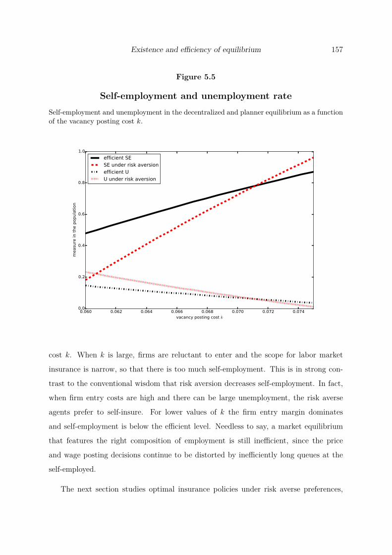
Existence and efficiency of equilibrium 157
Figure 5.5
Self-employment and unemployment rateSelf-employment and unemployment in the decentralized and planner equilibrium as a functionof the vacancy posting cost k.
0.060 0.062 0.064 0.066 0.068 0.070 0.072 0.074vacancy posting cost k
0.0
0.2
0.4
0.6
0.8
1.0
measu
re in t
he p
opula
tion
efficient SESE under risk aversionefficient UU under risk aversion
cost k. When k is large, firms are reluctant to enter and the scope for labor market
insurance is narrow, so that there is too much self-employment. This is in strong con-
trast to the conventional wisdom that risk aversion decreases self-employment. In fact,
when firm entry costs are high and there can be large unemployment, the risk averse
agents prefer to self-insure. For lower values of k the firm entry margin dominates
and self-employment is below the efficient level. Needless to say, a market equilibrium
that features the right composition of employment is still inefficient, since the price
and wage posting decisions continue to be distorted by inefficiently long queues at the
self-employed.
The next section studies optimal insurance policies under risk averse preferences,

158 Market theory of payroll and self-employment
when the market is not efficient. We investigate policies that make use of type-dependent
insurance and taxes to maximize output net of recruitment costs.
5.5. Efficient insurance policy
Having discussed the inefficiency of a market equilibrium under risk averse prefer-
ences, we now move towards an analysis of an efficient insurance policy. We consider
type-of-employment-dependent policies that satisfy the following definition:
Definition 5.4 (Balanced budget policies). A balanced budget policy is a tuple of taxes
and unemployment benefits P = {τSE, τLM , bSE, bLM} that satisfy the following condition:
bE (1 − µ (xLM)) LM + bSE (1 − aλ (xSE)) SE = τLMLM + τSESE. (5.1)
For analytical tractability, we illustrate the features of the policy under CARA pref-
erences with a risk aversion parameter θ:
u (c) = 1 − e−θc
θ.
Observe that the introduction of the policy instruments affects the price posting by self-
employed, wage posting by firms, and values of workers and self-employed, respectively.
These equations now read:
ϕ (xLM) [Aλ (xF ) pF − w]1 − ϕ (xLM)
= u (w − τLM) − u (bLM − τLM)u′ (w − τLM)
,
ϕ (xSE) (1 − pSE)1 − ϕ (xSE)
= u (pSE − τSE) − u (bSE − τSE)u′ (pSE − τSE)
,
V LM (P) = µ (xLM) u (w − τLM) + (1 − µ (xLM)) u (bLM − τLM) ,
V SE (P) = aλ (xSE) u (pSE − τSE) + (1 − aλ (xSE)) u (bSE − τSE) .
A natural question unfolds: is it possible to decentralize the planner equilibrium
using a balanced budget policy of type-of-employment-dependent taxes and unemploy-
ment benefits? The answer, as provided in the following proposition, is positive. More
interestingly, there is a clear pattern on how the unemployment benefits and otherwise
lump-sum taxes should be conditioned on the type of employment.

Efficient insurance policy 159
Proposition 5.4 (Efficient insurance policy). Let agents’ preferences be described by a
CARA utility function with a risk aversion parameter θ, and let there be a correspond-
ing equilibrium {x∗LM , w∗, x∗
SE, p∗SE, x∗
F , p∗F } denote the under risk neutral preferences.
Then there exists a balanced budget policy P∗ that for every θ decentralizes a planner
equilibrium such that:
bLM = w∗ − 1θ
log (1 + θw∗) ,
bSE = p∗SE − 1
θlog (1 + θp∗
SE) ,
V LM (P∗) = V SE (P∗) .
Moreover, the taxes are characterized by the following inequality:
τLM ≤ τSE ⇐⇒
log (1 + (1 − µ (x∗LM)) θw∗) − θw∗ ≥ log (1 + (1 − aλ (x∗
SE)) θp∗SE) − θp∗
SE.(5.2)
Proof. See Appendix 5.A.
It follows from the proof that the policy instruments separately target the three
margins of inefficiency. The unemployment insurance for the self-employed corrects
their pricing decision. The unemployment benefits for workers corrects the wage posting
decision. Finally, the mix of taxes ensures the correct composition of employment and
balances the budget.
Observe that whenever the price that prevails in the decentralized equilibrium under
risk neutrality is larger than the wage, the unemployment insurance for the self-employed
should be more generous. From the career choice indifference condition that implements
the efficient allocation we know that this happens if and only if the selling probability is
lower than the job finding probability. Thus, whenever the income from self-employment
is riskier, the benefits targeting the self-employed should be higher. This has nothing to
do, however, with risk sharing considerations and is solely driven by efficiency.
If θ is small, the ranking of the taxes in (5.2) can be approximated by
τLM ≤ τSE ⇐⇒ µ (x∗LM) w∗ ≤ aλ (x∗
SE) p∗SE,

160 Market theory of payroll and self-employment
so that self-employment should be taxed more heavily than labor market participation
whenever risk neutral individuals would prefer self-employment over entering the labor
market in an environment without taxation, given the unemployment benefits. When-
ever we find that bSE > bLM , which always happens if µ (x∗LM) > λ (x∗
SE), we may expect
to have τSE > τLM .
5.6. A dynamic model
In this section we describe the steady state of a dynamic version of the model, and
perform some comparative statics exercises. The dynamic model captures the idea that
employment at a firm is a long-term relationship. In particular, jobs last in expectation
for multiple periods and are destructed exogenously with a constant probability δ. Time
is discrete, individuals and buyers live forever, and they discount future periods at
a factor β. Self-employment’s and buyers’ outcomes are assumed independent across
periods. Therefore, the dynamic version of the model has consequences neither for
modeling self-employment and buyers, nor for the firms’ pricing decision. The value of
being a buyer is thus given by:
(1 − β) V B = η (xF ) (1 − pF ) = η (xSE) (1 − pSE) ,
while the value of the self-employed is given by
(1 − β) V SE = aλ (xSE) u (pSE) .
To minimize the differences with the static model, the timing of the model is such
that (1) existing jobs are destroyed, (2) vacancies enter, (3) individuals make their career
choice, (4) matches form, (5) buyers visit, and (6) individuals consume. To highlight the
time spent in unemployment within the model, we allow for an unemployment benefit.
As a result, the value of entering the labor market is equal to
V LM = µ (xLM) u (w) + (1 − µ (xLM)) u (b) + ... (5.1)
... + β[(1 − µ (xLM) (1 − δ)) V LM + µ (xLM) (1 − δ) V E
],

A dynamic model 161
with the value of employment V E being:
V E = u (w) + β[δV LM + (1 − δ) V E
].
Solving for V E and substituting the result in (5.1), it can be seen that the value of enter-
ing the labor market is still a weighted average of the expected time spent in employment
and in unemployment. As a result, the career choice is not so much different in the dy-
namic version of the model, and individuals are indifferent between self-employment and
entering the labor market if and only if
aλ (xSE) u (pSE) = µ (xLM) u (w) + (1 − µ (xLM)) (1 − β (1 − δ)) u (b)µ (xLM) + (1 − µ (xLM)) (1 − β (1 − δ))
.
The assumption that jobs in expectation last for multiple periods also affects firm
entry. The value of opening a vacancy is now
V V = −k + q (xLM) V J , (5.2)
where V J is the value of a filled vacancy (the value of a job to the firm):
V J = Aλ (xF ) pF − w + β (1 − δ) V J .
Solving for V J , substituting the result in (5.2), and closing the model by free entry
implies:
q (xLM) Aλ (xF ) pF − w
1 − β (1 − δ)= k (5.3)
As before, firms maximize expected profits by posting a wage, taking into account
its effect on xLM , constrained by the requirement to offer at least V LM to workers. As
shown in Appendix 5.B, this results in the following wage condition:
ϕ (xLM)1 − ϕ (xLM)
[Aλ (xF ) pF − w] = 1 − β (1 − δ)1 − β (1 − δ) (1 − µ (xLM))
u (w) − u (b)u′ (w)
.
Finally, we consider the stocks and flows of the dynamic model. Let Ft now denote
the measure of active firms at time t, and Vt the measure of vacancies opened in period
t. The flows are such that
Ft = q (xLM,t) Vt + (1 − δ) Ft−1,

162 Market theory of payroll and self-employment
Ut = (1 − µ (xLM,t)) (1 − SEt − (1 − δ)Et−1) ,
Et = µ (xLM,t) (1 − SEt − (1 − δ)Et−1) + (1 − δ) Et−1,
with the measure of active jobs Et = Ft, the measure of workers in period t equal to
1−SEt−(1−δ)Et−1, the queue length xLM,t = (1−SEt−(1−δ)Et−1)/Vt, and the measure
of labor market matches µ (xLM,t) (1 − SEt − (1 − δ)Et−1) = q (xLM,t) Vt. In steady state
the measure of self-employed is constant, and by definition 1−SE − (1− δ)E = U + δE,
so that the steady state satisfies:
q (xLM) V = δF = δE = µ (xLM) (U + δE) .
In Appendix 5.B, we show that for risk neutral preferences, the decentralized steady
state allocation of the dynamic model coincides with the steady state allocation that a
social planner would choose, if the planner maximizes the present discounted number
of goods sold net of recruiting costs. The social planner then solves the following op-
timisation problem of deciding on the type of employment choice, firm entry and the
allocation of buyers:
max{xSE,t,Vt,Et,SEt}∞
t=1
∞∑t=1
βt [xF,tη (xF,t) AEt + xSE,tη (xSE,t) aSEt − Vtk] ,
subject to:
Et = q (xLM,t) Vt + (1 − δ)Et−1,
and an initial condition E0, where xLM,t = (1−SEt−(1−δ)Et−1)/Vt from the unit mass of
households, the career choice, and job survival, and where xF,t = (1 − xSE,taSEt)/(AEt)
from the accounting identity in the goods market. In every period we again allow the
social planner to choose the measure of vacancies to be opened and the measure of
households to enter self-employment (and thus the measure to enter the labor market).
The social planner still faces the same visibility probabilities and coordination frictions
within every (sub)market as present in the decentralized equilibrium, but can still decide
upon the measure of buyers to go shopping at the self-employed (and thus the measure
of buyers that visits firms). Finally, note that choosing the latter, given SEt and Vt,

Conclusions 163
still amounts to choosing xSE,t, because the only state variable Et is also determined by
SEt and Vt (and Et−1). Since the decentralized and the planner’s allocation coincide,
the equilibrium of the dynamic model is efficient when individuals are risk neutral, just
as the static model.
On the one hand, the steady state of a dynamic version of the model is not so much
different from the static model, because the the value of entering the labor market is still
a weighted average of the expected time spent in employment and in unemployment. On
the other hand, the dynamic model captures the idea that jobs last for multiple periods
and introduces two additional parameters: patience, and the expected duration of the
wage contract. In Figure 5.6 we show the response of the equilibrium self-employment
rate to changes in the discount factor β and the job destruction probability δ. Not
surprisingly, a higher discount factor and lower job separation probability make the
long-term nature of a wage contract more valuable to individuals, which decreases the
self-employment rate.
5.7. Conclusions
We propose a new theory of self-employment that emphasizes the trade-off between
the frictions in the goods and in the labor market. Our theory, unlike a vast body of
earlier research, does not rely on individual heterogeneity. It also offers microfoundations
for the differences in the riskiness of payroll and self-employment incomes. In our model
the self-employed forego coordination frictions in the labor market and the sharing of
the match surplus with the firm. They are exposed, however, to coordination frictions
in the goods market.
We also show that the decentralized equilibrium is inefficient if individuals are risk
averse. In this case explicitly modeling trade in the goods market is crucial, as risk
averse self-employed steal business from risk neutral firms by charging low prices. This
under-pricing is a form of self-insurance, which reduces output sold net of recruiting
costs. Interestingly, we show that in this environment unemployment insurance for self-

164 Market theory of payroll and self-employment
Figure 5.6
Comparative statics in dynamic modelEquilibrium self-employment rate as a function of β and δ.
0.90 0.91 0.92 0.93 0.94 0.95discount factor β
0.1
0.2
0.3
0.4
0.5
self-e
mplo
ym
ent
rate
0.05 0.06 0.07 0.08 0.09 0.10firm-employee separation rate δ
0.1
0.2
0.3
0.4
0.5
self-e
mplo
ym
ent
rate
employed individuals can improve efficiency, because it decreases the incentives to self-
insure. As a result, firm entry increases and prospects in the labor market improve. Such
insurance can therefore increase output sold net of recruiting costs, while simultaneously
sharing risks.
5.A: Proofs for the static model
Proof of Lemma 5.1 (Optimal price posting).
The self-employed post prices to maximize their expected utility as given in (5.2),
offering buyers at least their value V B as given in (5.1). Using the latter, the price that

Proofs for the static model 165
the self-employed post can be written as a function of V B and xSE:
pSE = 1 − V B
η (xSE).
Substituting out pSE, the self-employed problem can then be written as a choice op the
optimal queue length:
maxxSE
axSEη (xSE) u
(1 − V B
η (xSE)
).
The first-order condition yields:
aη (xSE) u (pSE) + axSEη′ (xSE) u (pSE) + axSEη (xSE) u′ (pSE) ∂pSE
∂η (xSE)η′ (xSE) = 0.
Dividing by aη (xSE) gives:
(1 − ϕ (xSE)) u (pSE) − η (xSE) ϕ (xSE) u′ (pSE) ∂pSE
∂η (xSE)= 0
Using that ∂pSE
∂η(xSE) = V B
η2(xSE) , and substituting out V B, we get:
(1 − ϕ (xSE)) u (pSE) = ϕ (xSE) u′ (pSE) (1 − pSE) , (5.A.1)
which is equal to (5.3). The price-posting problem of firms is the same, except that firms
maximize expected revenue instead of utility. Replacing u (pSE) by pF and u′ (pSE) by
1 results in (5.4).
Proof of Lemma 5.2 (Optimal wage posting).
After paying an entry cost k, the firm optimally chooses the queue length to maximize
profits
Π = q (xLM) (Aλ (xF ) pF − w) ,
subject to the market utility of workers V LM as given in (5.5). Via this outside option,
the wage to be paid also depends on xLM , so that the first-order condition is
q′ (xLM) (Aλ (xF ) pF − w) − q (xLM) dw
dxLM
= 0.

166 Market theory of payroll and self-employment
The derivative of the wage is obtained from totally differentiating V LM , which is fixed:
0 = µ′ (xLM) u (w) + µ (xLM) u′ (w) dw
dxLM
,
so that the optimality condition reads
q′ (xLM) (Aλ (xF ) pF − w) = −q (xLM) µ′ (xLM)µ (xLM)
u (w)u′ (w)
.
Finally, note that −xLM µ′(xLM )µ(xLM ) = 1 − ϕ (xLM), and (5.6) results.
Proof of Proposition 5.1 and Corollary 5.1 (Existence of equilibrium and
comparative statics).
The mixing condition in (5.1) can be obtained by combining (5.1) with the first con-
dition of Definition 5.3. It follows that limaxSE 7→1− LM = 0+ and limAxF µ(xLM )7→1+ LM =
1− as long as the denominator of (5.1) is not approaching zero and is positive. Then,
we can substitute out prices and the wage out of the remaining six equilibrium condi-
tions, so that - together with the mixing condition - we are left with the following three
equations in three unknowns {xSE, xF , xLM}:
ϕ (xLM)[
kq(xLM )
]1 − ϕ (xLM)
=u(Aλ (xF ) ϕ (xF ) − k
q(xLM )
)u′(Aλ (xF ) ϕ (xF ) − k
q(xLM )
) (5.A.2)
µ (xLM) u
(Aλ (xF ) ϕ (xF ) − k
q (xLM)
)= (5.A.3)
= aλ (xSE) u
(1 − η (xF ) (1 − ϕ (xF ))
η (xSE)
)ϕ (xSE)
(η(xF )(1−ϕ(xF ))
η(xSE)
)1 − ϕ (xSE)
=u(1 − η(xF )(1−ϕ(xF ))
η(xSE)
)u′(1 − η(xF )(1−ϕ(xF ))
η(xSE)
) . (5.A.4)
Existence and uniqueness follow from invoking the Implicit Function Theorem on this
system of equations. To demonstrate the logic of the proof, we prove the risk neutral
case first. Afterwards we show that the same argument applies for CRRA preferences.
Risk neutral preferences. For risk neutral preferences, (5.A.4) boils down to e−xSE =
e−xF , so that xF = xSE, which echoes the fact that risk neutral self-employed and firms

Proofs for the static model 167
set the same prices. Then, (5.A.3) implies xLM = log (A/a), as in (5.11). The mixing
condition can now be restated as
0 <1 − axSE(
A−a
log(Aa ) − a
)xSE
< 1,
which places bounds on xSE. In particular, for 1 > LM > 0, it must hold that 1/a >
xSE >log(A
a )A−a
, which can only be true ifA
a> 1 + log
(A
a
). (5.A.5)
Observe that this condition - the first inequality constraint on the exogenous parameters
to have a mixed strategy equilibrium - also guarantees that the share of prospective
workers LM is non-negative and finite. Besides, note that condition (5.A.5) is always
satisfied if A > a.
Equation 5.A.2 - the only equilibrium condition that is left - can after manipulation
and evaluation at xLM = log (A/a) be defined as
h (xSE, a, A, k) ≡A − a − a log
(Aa
)A
(1 − xSEe−xSE − e−xSE
)− k = 0. (5.A.6)
Differentiating (5.A.6), we find the following relationships:
∂h
∂xSE
=A − a − a log
(Aa
)A
xSEe−xSE > 0,
∂h
∂k= −1 < 0,
∂h
∂A= a
A2 log(
A
a
)(1 − xSEe−xSE − e−xSE
)> 0,
∂h
∂a= − 1
Alog
(A
a
) (1 − xSEe−xSE − e−xSE
)< 0.
Thus, from the Implicit Function Theorem we get, in particular, that ∂xSE
∂k> 0. Then,
the bounds for the mixed strategy equilibrium to exist follow from evaluating (5.A.6) at
xSE 7→ 1a
− to get k (A, a) and xSE 7→ log(Aa )
A−a
+to get k (A, a).
The comparative statics of the self-employment rate follow from total differentiation
of the accounting identity on individuals:∂SE∗
∂k= −∂LM∗
∂k.

168 Market theory of payroll and self-employment
To find the latter, we make use of chain rule: ∂LM∗
∂k= ∂LM∗
∂xSE
∂xSE
∂k. From the Implicit
Function Theorem applied to (5.A.6), we have that ∂xSE
∂k> 0. The derivative of LM∗
with respect to xSE reads−(
A−a
log(Aa ) − a
)[(
A−a
log(Aa ) − a
)xSE
]2 < 0,
which implies that
∂SE∗
∂k= − ∂LM∗
∂xSE︸ ︷︷ ︸<0
>0︷ ︸︸ ︷∂xSE
∂k> 0.
The derivatives of bounds on k, k (A, a) and k (A, a), with respect to A and a also
follow from the Implicit Function Theorem:
∂k
∂A= −
∂h∂k∂h∂A
> 0,
∂k
∂a= −
∂h∂k∂h∂a
< 0.
Preferences with risk aversion. We show that the argument above applies to the
more general case case of u (c) = c1−γ
1−γwith γ ∈ [0, 1], so that now u(c)
u′(c) = c1−γ
. From
(5.A.4), the price posting by the self-employed then leads to the following relationship
between queue lengths in the mixed strategy equilibrium:
xF = xSE + log (1 − γϕ (xSE)) .
Observe that this implies xF = xSE if and only if γ = 0. Otherwise, we have that
xF < xSE whenever the mixed strategy equilibrium exists, and this ratio is decreasing
in risk aversion parameter γ. Reformulating (5.A.4) and (5.A.4), we then have two
equations with two unknowns xLM and xSE:
(1 − γ) ϕ (xLM)[
kq(xLM )
]1 − ϕ (xLM)
= Aλ (xF ) ϕ (xF ) − k
q (xLM)(5.A.7)
µ (xLM)(
Aλ (xF ) ϕ (xF ) − k
q (xLM)
)1−γ
= aλ (xSE)(
1 − η (xF ) (1 − ϕ (xF ))η (xSE)
)1−γ
(5.A.8)

Proofs for the static model 169
We can further simplify (5.A.7) to
k
q (xLM)= Aλ (xF ) ϕ (xF )
[1 − ϕ (xLM)
1 − γϕ (xLM)
],
so that (5.A.8) becomes
µ (xLM)(
Aλ (xF ) ϕ (xF ) (1 − γ) ϕ (xLM)1 − γϕ (xLM)
)1−γ
= aλ (xSE)(
1 − η (xF ) (1 − ϕ (xF ))η (xSE)
)1−γ
.
Now we set this equation to zero and define it as z (xLM , xSE) = 0. Collecting terms,
taking logs and differentiating, results in:
∂z
∂xLM
= µ′ (xLM)µ (xLM)
+ (1 − γ) ϕ′ (xLM)ϕ (xLM) (1 − γϕ (xLM))
< 0 whenever xLM = 0.
The part of z (xLM , xSE) that is relevant for computing ∂z∂xSE
reads:
z (xLM , xSE) = log(
λ (xF )λ (xSE)
)− γ log (λ (xF )) + (1 − γ) log
(pF
pSE
).
Under risk neutrality, γ = 0 and we have that the derivative of z with respect to xSE is
zero which also implies that xLM does not respond to xSE. After some tedious algebra
one can show that∂z
∂xSE
< 0,
which also implies that there exists a function xLM (xSE), decreasing in its argument.
From here we can already establish the existence of equilibrium bounds on k, as the
right hand side of identity:
k = q (xLM) Aλ (xF ) ϕ (xF )[
1 − ϕ (xLM)1 − γϕ (xLM)
],
is strictly increasing in xSE so that the logic of the existence proof for the risk neutral
preferences carries over.
Proof of Proposition 5.3 (Efficiency of equilibrium).
Using the accounting identity in (5.1), the planner’s objective can be written as:
V SP (V, xSE, SE) = xSEaSE (η (xSE) − η (xF )) + η (xF ) − V k. (5.A.9)

170 Market theory of payroll and self-employment
For future reference, note that the partial derivatives of xF with respect to the choice
variables of the social planner are given by:
∂xF
∂V= xF
V(ϕ (xLM) − 1) ,
∂xF
∂xSE
= − aSE
Aq(xLM)V,
∂xF
∂SE= xF Aq′ (xLM) − axSE
Aq(xLM)V.
Taking the first order condition with respect to the measure of firms:
∂V SP
∂V= η′ (xF ) ∂xF
∂V(1 − xSEaSE) − k = 0,
= η′ (xF ) (xF )2 Aq (xLM) (ϕ (xLM) − 1) − k = 0,
= (1 − ϕ (xLM)) Aq (xLM) λ (xF ) ϕ (xF ) − k = 0,
which is exactly the free entry condition in the decentralized equilibrium if workers are
risk neutral as given in (5.8), since firms always post pF = ϕ (xF ).
Let ∆η ≡ η (xSE)−η (xF ). Taking the first order condition with respect to the queue
length at the self-employed:
∂V SP
∂xSE
= SEa∆η + xSEaSEη′ (xSE) + (1 − xSEaSE) η′ (xF ) ∂xF
∂xSE
= 0,
= η (xSE) (1 − ϕ (xSE)) − η (xF ) (1 − ϕ (xF )) = 0,
which (only) for risk neutral self-employed is exactly the buyer indifference condition in
the goods market as in (5.1), since they post pSE = ϕ (xSE) (and firms post pF = ϕ (xF )).
Finally, the first order condition with respect to the measure of self-employed:
∂V SP
∂SE= xSEa∆η + (1 − xSEaSE) η′ (xF ) ∂xF
∂SE= 0,
= xSEa∆η + xF η′ (xF ) (xF Aq′ (xLM) − xSEa) = 0,
= ∆η + η (xF ) ϕ (xF )(
1 − xF Aq′ (xLM)xSEa
)= 0,
= η (xSE)(
1 − xF η (xF ) Aq′ (xLM) ϕ (xF )xSEaη (xSE)
)− η (xF ) (1 − ϕ (xF )) = 0.

Proofs for the static model 171
This equation is equal to the buyer indifference condition in the goods market if
ϕ (xSE) = Aλ (xF ) q′ (xLM) ϕ (xF )aλ (xSE)
,
which is exactly the condition that makes risk neutral households indifferent between
entering the goods market as self-employed on the one hand and entering the labor
market on the other. Indeed, it makes V LM as given in (5.9) equal to (5.2) when
self-employed post pSE = ϕ (xSE). Hence, risk neutrality is sufficient for constrained
efficiency.
Now, let us assume that in the decentralized allocation we have the measure of
firms, the composition of employment, and the queues in the goods market that coincide
with the planner solution. In other words, we assume that the decentralized allocation
{V ∗, SE∗, x∗SE} exactly matches its planner counterpart
{V SP , SESP , xSP
SE
}. Then, let
us assume that individuals are risk averse. Given that xSPSE = x∗
SE, we can directly
compare p∗SE and the pSP
SE = ϕ (xSE) that decentralizes the planner’s solution. From the
optimal price posting condition we get that under risk aversion pSPSE = p∗
SE, which implies
that the buyers’ indifference condition is violated: the buying probabilities equal their
counterparts from the planner’s solution, but the buyers have an incentive to choose
visits at the self-employed more often. Thus, one of the planner’s solution conditions is
violated. This demonstrates the necessity of the risk neutrality assumption.
Consequently, the decentralized allocation is maximizing net output sold if and only
if individuals are risk neutral.
Proof of Proposition 5.4 (Efficient insurance policy).
Formally, we consider policies that have to satisfy the balanced-budget identity:
bLM (1 − µ (xLM)) LM + bSE (1 − aλ (xSE)) SE = τLMLM + SEτSE. (5.A.10)
The introduction of taxes and insurance changes the wage posting by firms and the price
posting by the self-employed. These equations now read:ϕ (xLM) [Aλ (xF ) pF − w]
1 − ϕ (xLM)= u (w − τLM) − u (bLM − τLM)
u′ (w − τLM),

172 Market theory of payroll and self-employment
ϕ (xSE) (1 − pSE)1 − ϕ (xSE)
= u (pSE − τSE) − u (bSE − τSE)u′ (pSE − τSE)
.
Observe that the taxes themselves are not relevant in the pricing/wage posting deci-
sion, as they affect agents’ wealth in all states (employed/unemployed/selling/not sell-
ing). Because CARA preferences feature no wealth effect, τi drop out. They do matter,
however, in making the relative comparison of the career choices available. Starting with
pricing by the self-employed:
ϕ (xSE) (1 − pSE)1 − ϕ (xSE)
= 1θ
e−θ(bSE−τSE) − e−θ(pSE−τSE)
e−θ(pSE−τSE) = 1θ
(e−θ(bSE−pSE) − 1
).
Now, suppose we wish to find bSE that implements pSE = ϕ (x∗SE) with the queue
length as in the (efficient) allocation under risk neutral preferences. Then, it has to
satisfy the following condition:
bSE = ϕ (x∗SE) − 1
θlog (1 + θϕ (x∗
SE)) .
The wage posting works in an analogous way, namely:
ϕ (xLM) [Aλ (xF ) pF − w]1 − ϕ (xLM)
= 1θ
(e−θ(bLM −w) − 1
).
Let’s do the same for bLM . The efficient wage satisfies w = ϕ (x∗LM) Aλ (x∗
F ) p∗F so
that:
ϕ (x∗LM) Aλ (x∗
F ) p∗F = 1
θ
(e−θ(b∗
LM −w∗) − 1)
bLM = ϕ (x∗LM) Aλ (x∗
F ) p∗F − 1
θlog (1 + θϕ (x∗
LM) Aλ (x∗F ) p∗
F )
Observe, that these conditions have an easy interpretation, namely:
bLM = w∗ − 1θ
log (1 + θw∗)
bSE = p∗SE − 1
θlog (1 + θp∗
SE)

Proofs for the static model 173
The worker indifference condition reads:
V LM = V SE with:
V LM = µ (xLM) u (w − τLM) + (1 − µ (xLM)) u (bLM − τLM)
V SE = aλ (xSE) u (pSE − τSE) + (1 − aλ (xSE)) u (bSE − τSE)
so that:
µ (xLM) u (w − τLM) + (1 − µ (xLM)) u (bLM − τLM) =
aλ (xSE) u (pSE − τSE) + (1 − aλ (xSE)) u (bSE − τSE) .
With u (c) = 1−e−θc
θ, we arrive at the following:
µ (xLM) e−θ(w−τLM ) + (1 − µ (xLM)) e−θ(bLM −τLM ) =
aλ (xSE) e−θ(pSE−τSE) + (1 − aλ (xSE)) e−θ(bSE−τSE)
so that:eθτLM
eθτSE= aλ (xSE) e−θpSE + (1 − aλ (xSE)) e−θbSE
µ (xLM) e−θw + (1 − µ (xLM)) e−θbLM
Using the analytical expressions for bLM and bSE we can rewrite the career choice equa-
tion as:
θτLM − θw∗ + log (1 + (1 − µ (x∗LM)) θw∗) = θτse − θp∗
SE + log (1 + (1 − aλ (x∗SE)) θp∗
SE) .
The taxes can therefore be ranked such that
τLM < τSE ⇐⇒ log (1 + (1 − µ (x∗LM)) θw∗)−θw∗ > log (1 + (1 − aλ (x∗
SE)) θp∗SE)−θp∗
SE.
Proof of the knife-edge condition
Whatever the price in the goods market is, it’s the same for all the sellers and thus
can be normalised to 1. Now, the wage posting condition implies
w = xwe−xw
1 − e−xwA.

174 Market theory of payroll and self-employment
The worker indifference condition requires:
1 − e−xw
xw
w = a
which together with the first equation gives us:
a
A= e−xw .
Finally, the free entry condition is:
k =(1 − e−xw
)(A − w) .
Putting this together with the wage posting condition we get:
k =(1 − e−xw − xwe−xw
)A
so that:k
A= 1 − a
A+ a
Alog
(a
A
)to finally get
k
A= 1 − a
A
(1 − log
(a
A
))
5.B: Proofs for the dynamic model
Optimal wage posting under general preferences
To derive the wage condition under general preferences, let firms maximize the left-
hand side of the free-entry condition:
ϕ (xLM) [Aλ (xF ) pF − w]1 − ϕ (xLM)
= u (w) − (1 − β (1 − δ)) u (b) − β (1 − δ) (1 − β) V LM
u′ (w),
=(
1 − β (1 − δ) µ (xLM)µ (xLM) + (1 − µ (xLM)) (1 − β (1 − δ))
)u (w) − u (b)
u′ (w),
= 1 − β (1 − δ)1 − β (1 − δ) (1 − µ (xLM))
u (w) − u (b)u′ (w)
.

Proofs for the dynamic model 175
Risk-neutral individuals
If workers are risk neutral and bSE = 0, then the optimal wage posting simplifies to
ϕ (xLM)1 − ϕ (xLM)
[Aλ (xF ) pF − w] = 1 − β (1 − δ)1 − β (1 − δ) (1 − µ (xLM))
w,
ϕ (xLM) Aλ (xF ) pF [1 − β (1 − δ) (1 − µ (xLM))] = [1 − β (1 − δ) (1 − µ (xLM) ϕ (xLM))] w,
w = ϕ (xLM) Aλ (xF ) pF [1 − β (1 − δ) (1 − µ (xLM))]1 − β (1 − δ) (1 − µ (xLM) ϕ (xLM))
. (5.B.1)
Under these conditions, the value of entering the labor market is given by
(1 − β)V LM = µ (xLM) w
1 − β (1 − δ) (1 − µ (xLM)),
so that individuals are indifferent between careers if and only if
[1 − β (1 − δ) (1 − µ (xLM))] aλ (xSE) pSE = µ (xLM) w. (5.B.2)
Substituting the wage of (5.B.1) in this individuals’ indifference condition, yields:
aλ (xSE) pSE = µ (xLM) ϕ (xLM) Aλ (xF ) pF
1 − β (1 − δ) (1 − µ (xLM) ϕ (xLM)). (5.B.3)
Finally, substituting the wage of (5.B.1) in the free entry condition of (5.3), yields:[Aλ (xF ) pF − ϕ (xLM) Aλ (xF ) pF [1 − β (1 − δ) (1 − µ (xLM))]
1 − β (1 − δ) (1 − µ (xLM) ϕ (xLM))
]= k [1 − β (1 − δ)]
q (xLM),
q (xLM) Aλ (xF ) pF[1 − β (1 − δ)] (1 − ϕ (xLM))
1 − β (1 − δ) (1 − µ (xLM) ϕ (xLM))= k [1 − β (1 − δ)] ,
q (xLM) Aλ (xF ) pF (1 − ϕ (xLM))1 − β (1 − δ) (1 − µ (xLM) ϕ (xLM))
= k. (5.B.4)
Efficiency
Using xF,t = 1−xSE,taSEt
AEt, and defining ∆ηt ≡ η (xSE,t) − η (xF,t), simplifies the objec-
tive of the social planner to:
max{xSE,t,Vt,Et,SEt}∞
t=1
∞∑t=1
βt [xSE,taSEt∆ηt + η (xF,t) − Vtk] . (5.B.5)

176 Market theory of payroll and self-employment
Choosing xSE,t is only an intra-temporal problem, but both SEt and Vt determine future
values of employment E. For that reason, we set up a Lagrangian:
L =∞∑
t=1
{βt [xSE,taSEt∆ηt + η (xF,t) − Vtk] + νt [q (xLM,t) Vt + (1 − δ)Et−1 − Et]
},
where νt is the Lagrange multiplier on the law of motion for Et.
The first-order condition with respect to xSE,t is
∂L∂xSE,t
= βt[aSEt∆ηt + xSE,taSEt
(η′ (xSE,t) + η′ (xF,t)
aSEt
AEt
)− η′ (xF,t)
aSEt
AEt
]= 0,
= aSEt∆ηt + aSEtxSE,tη′ (xSE,t) − aSEtxF,tη
′ (xF,t) = 0,
= η (xSE,t) (1 − ϕ (xSE,t)) − η (xF,t) (1 − ϕ (xF,t)) = 0, (5.B.6)
which is the same intra-temporal condition for the goods market as in the static model.
If the self-employed are risk neutral, then pSE,t = ϕ (xSE,t). Together with the price-
setting of firms, this condition then coincides with the buyers’ indifference condition of
the decentralized allocation as given above. Consequently, the decentralized allocation
in the goods market is efficient if individuals are risk neutral.
The first-order condition with respect to Vt is
∂L∂Vt
= −βtk + νt [q (xLM,t) − q′ (xLM,t) xLM,t] = 0, (5.B.7)
βtk
q (xLM,t) (1 − ϕ (xLM,t))= νt. (5.B.8)
The first-order condition with respect to Et is
∂L∂Et
= βtη′ (xF,t)xF,t
Et
[xSE,taSEt − 1] − νt + νt+1 [(1 − δ) − q′ (xLM,t) (1 − δ)] = 0,
= −βtη′ (xF,t) Ax2F,t − νt + νt+1 (1 − δ) (1 − ϕ (xLM,t) µ (xLM,t)) = 0,
= βtAλ (xF,t) ϕ (xF,t) − νt + νt+1 (1 − δ) (1 − ϕ (xLM,t) µ (xLM,t)) = 0.
Substituting (5.B.8), yields
βtAλ (xF,t) ϕ (xF,t) = βtk
q (xLM,t) (1 − ϕ (xLM,t))− βt+1k (1 − δ) (1 − ϕ (xLM,t) µ (xLM,t))
q (xLM,t+1) (1 − ϕ (xLM,t+1)),

Proofs for the dynamic model 177
k = q (xLM,t) (1 − ϕ (xLM,t)) Aλ (xF,t) ϕ (xF,t)
1 − q(xLM,t)(1−ϕ(xLM,t))q(xLM,t+1)(1−ϕ(xLM,t+1))β (1 − δ) (1 − ϕ (xLM,t) µ (xLM,t))
,
which is a first-order difference equation for optimal entry. In steady state the ratio of
today’s and tomorrow’s matching rates and elasticities is equal to one, and this equation
simplifies to
k = q (xLM) Aλ (xF ) ϕ (xF ) (1 − ϕ (xLM))1 − β (1 − δ) (1 − µ (xLM) ϕ (xLM))
, (5.B.9)
which equals the free entry condition in (5.B.4) given that pF = ϕ (xF ). Consequently,
free entry in the decentralized allocation is optimal if wages are set for the case that
workers are risk neutral.
The first-order condition with respect to SEt is
∂L∂SEt
= βt
[xSE,ta∆ηt +
x2SE,taSEtη
′ (xF,t)AEt
− η′ (xF,t) xSE,ta
AEt
]− νtq
′ (xLM,t) = 0,
= βt [xSE,ta∆ηt − xSE,taxF,tη′ (xF,t)] − νtµ (xLM,t) ϕ (xLM,t) = 0,
= βtxSE,ta [η (xSE,t) − η (xF,t) (1 − ϕ (xF,t))] − νtµ (xLM,t) ϕ (xLM,t) = 0.
Substituting (5.B.8) and rearranging, results in
βtxSE,ta [η (xSE,t) − η (xF,t) (1 − ϕ (xF,t))] = βtkµ (xLM,t) ϕ (xLM,t)q (xLM,t) (1 − ϕ (xLM,t))
,
η (xSE,t) − η (xF,t) (1 − ϕ (xF,t)) = η (xSE,t) kµ (xLM,t) ϕ (xLM,t)aλ (xSE,t) q (xLM,t) (1 − ϕ (xLM,t))
,
η (xSE,t)(
1 − kµ (xLM,t) ϕ (xLM,t)aλ (xSE,t) q (xLM,t) (1 − ϕ (xLM,t))
)= η (xF,t) (1 − ϕ (xF,t)) ,
which coincides with the goods market condition in (5.B.6) if and only if
ϕ (xSE,t) = kµ (xLM,t) ϕ (xLM,t)aλ (xSE,t) q (xLM,t) (1 − ϕ (xLM,t))
.
Using the steady state optimal firm entry decision in (5.B.9) to substitute for k,
aλ (xSE,t) ϕ (xSE,t) = µ (xLM,t) ϕ (xLM,t) q (xLM,t) Aλ (xF,t) ϕ (xF,t) (1 − ϕ (xLM,t))q (xLM,t) (1 − ϕ (xLM,t)) [1 − β (1 − δ) (1 − µ (xLM,t) ϕ (xLM,t))]
,
= µ (xLM,t) ϕ (xLM,t) Aλ (xF,t) ϕ (xF,t)1 − β (1 − δ) (1 − µ (xLM,t) ϕ (xLM,t))
.

178 Market theory of payroll and self-employment
Given that firms set pF = ϕ (xF,t) and that risk neutral self-employed set pSE = ϕ (xSE,t),
this is exactly the individuals’ indifference condition in the career choice game if they
are risk neutral, as can be seen in (5.B.3). Consequently, also the career choice of risk
neutral individuals maximizes total output sold. We conclude that {xSE,t, Vt, Et, SEt}∞t=1
are chosen efficiently by the market.

Summary
This book consists of four self-contained essays in macroeconomics with a special focus
on international economics and labour economics. The common theme of this research is
the role of information frictions and micro level heterogeneity in shaping of the macroe-
conomic aggregates. The first two chapters focus on pitfalls and perils of cross-country
financial integration, while the other two chapters investigate the drivers and conse-
quences of career choice between payroll- and self-employment.
Chapter 2, Public Data Quality and International Risk Sharing, documents striking
relationship between the quality of public information and cross-country risk sharing. We
document that certain countries with good quality data and efficient statistical agencies
receieve less insurance against fluctuations in their GDP growth rate than countries
that either do much better or much worse in terms of the quality of data they supply
to the general public. Standard theories of borrowing and lending when applied to
cross-country consumption and GDP data predict that the relationship between public
information quality and insurance was monotone. It should be either strictly increasing,
if the set of available securities is incomplete, or strictly decreasing when there were no
constraints on available assets.
We provide a theoretical model that can replicate the pattern found in the data.
Our key novelty is that we also account for countries transparency. Hence, a country
can provide very narrow, but high quality data to the general public, withhelding parts
of the data due to either institutional lags, legal reasons or for political gain. Thus,
high quality public information may coexist with various degrees of withheld private
179

information. The interaction of the two is the source of non-monotone relationship
between data quality and cross-country insurance. The more precise withheld private
information is, the more difficult it is for a country to negotiate terms of its borrowing
and lending. If private information is sufficiently precise, public information improves
risk sharing by reducing the adverse selection problem.
In our quantitative exercise we demonstrate that efforts towards improving publicly
available data by, say, the IMF or the World Bank are dwarved by effects of individual
countries move towards more transparency, thus revealing more of their privately stored
information to the world.
In Chapter 3, Monetary Policy and Foreign-Owned Banks in Emerging Economies,
we investigate the effects of banking system penetration by foreign owned banks in
Central and Eastern Europe economies. Ongoing political debate points towards perils
of uncontrolled cross-country capital flows which can be perilous especially in times of
financial crisis and calls for increased scrutiny of foreign banks subsidiaries.
We look at the differences in the type of bank ownership and the conduct of monetary
policy. We find that foreign-owned banks are less-responsive to host country monetary
policy. This finding at first glance supports the narrative of increase in exposure to risk
in emerging economies that comes from financial integration. However, when we dissect
this effect we find that it is fully explained by higher foreign owned banks profitability.
Thus, our findings suggest that the tamed response of these banks to monetary policy is
not necessarily a manifestation of hidden threat of sudden capital outflow. It is rather
coming from competitive advantage of foreign banks over domestic banks.
In Chapter 4, A Model of Confounded Entrepreneurial Choice, I build a model of
labour market learning that aims at understanding frequent switches between payroll
and self-employment of young workers. This chapter reconciles the switching behaviour
with other studies that document a sizeable fraction of entrepreneurs persistently earn
less than what they would be earning as employees with similar characteristics.

In my model earnings in entrepeneurship and payroll employment are correlated, as
individual abilities that determine employee earnings, are also supplied in entrepreneur-
ship and determine entrepreneurial outcomes jointly with the business idea. However,
entrepreneurs can’t disentangle the two, as they only observe the income their business
generates. Because of that, an underperforming entrepreneur might confuse the negative
quality of the business idea with low own ability, postponing return to payroll employ-
ment. Thus, because of a more complicated learning problem, entrepreneurs may suffer
from a lock-in effect. This finding provides an alternative to the non-pecuniary benefits
of being one’s own boss. My model suggest that reducing uncertainty about individual
ability through internships and payroll jobs improves selection into entrepreneurship.
Finally, Chapter 5, Efficient insurance in market theory of payroll and self-employment,
continues to investigate the choice between payroll- and self-employment but it focuses
on the role of goods market frictions. We show that it is possible to think of this choice as
a randomisation of identical workers who trade the risk of not finding a job and sharing
the surplus of the match with a firm against the risk of not finding a consumer on their
own when self-employed. The key driver force of our model are differentiated business
conditions, like productivity or ease of finding customers by firms and self-employed.
Thus, our theory may explain the fraction of probability of selecting into each of the
two types of employment that is not captured by differences in gender, education and
alike and speaks well to the increase of the so called ‘gig-economy’ and the prevalence
of ‘tap-workers’.
In our model, if workers’ preferences feature aversion towards risk, the market equi-
librium is inefficient, because wages paid by the firms are too low, but also because the
self-employed down-price their good attracting inefficiently many customers given their
production capacities. We show that there should be unemployment benefits for unem-
ployed together with income support for self-employed who fail to generate income to
ameliorate the inefficiency. Financing of such an insurance scheme also requires trans-
fers between the two types of employment via differentiated taxes. Thus, our theory

provides rationale for benefit policies introduced recently in Denmark and Sweden.

Bibliography
Acemoglu, D. and R. Shimer (1999): “Efficient Unemployment Insurance,” Journal
of Political Economy, 107, 893–928.
Adams-Kane, J., J. A. Caballero, and J. J. Lim (2013): “Foreign bank behavior
during financial crises,” Policy Research Working Paper Series 6590, The World Bank.
Allen, F., K. Jackowicz, and O. Kowalewski (2013): “The effects of foreign
and government ownership on bank lending behavior during a crisis in Central and
Eastern Europe,” MPRA Paper 48059, University Library of Munich, Germany.
Arellano, C. (2008): “Default Risk and Income Fluctuations in Emerging
Economies,” American Economic Review, 98, 690–712.
Arellano, M. and S. Bond (1991): “Some Tests of Specification for Panel Data:
Monte Carlo Evidence and an Application to Employment Equations,” Review of
Economic Studies, 58, 277–97.
Arellano, M. and O. Bover (1995): “Another look at the instrumental variable
estimation of error-components models,” Journal of Econometrics, 68, 29 – 51.
Atkeson, A. and R. E. Lucas (1992): “On Efficient Distribution with Private In-
formation,” Review of Economic Studies, 59, 427–453.
——— (1995): “Efficiency and Equality in a Simple Model of Efficient Unemployment
Insurance,” Journal of Economic Theory, 66, 64–88.
183

Aydin, B. (2008): “Banking Structure and Credit Growth in Central and Eastern
European Countries,” IMF Working Papers 08/215, International Monetary Fund.
Bai, Y. and J. Zhang (2012): “Financial integration and international risk sharing,”
Journal of International Economics, 86, 17–32.
Baron, R. A. (1998): “Cognitive mechanisms in entrepreneurship: Why and when
enterpreneurs think differently than other people,” Journal of Business Venturing,
13, 275 – 294.
Baxter, M. (2011): “International Risk Sharing in the Short Run and in the Long
Run,” NBER Working Papers 16789, National Bureau of Economic Research, Inc.
Bernanke, B. S. and A. S. Blinder (1992): “The Federal Funds Rate and the
Channels of Monetary Transmission,” American Economic Review, 82, 901–21.
Bertsekas, D. P. and S. E. Shreve (2007): Stochastic Optimal Control: The
Discrete-Time Case, Athena Scientific.
Blackwell, D. (1953): “Equivalent comparisons of experiments,” Ann. Math. Stat.,
24, 265–272.
Blundell, R. and S. Bond (1998): “Initial conditions and moment restrictions in
dynamic panel data models,” Journal of Econometrics, 87, 115 – 143.
Bonin, J. P., I. Hasan, and P. Wachtel (2005): “Bank performance, efficiency
and ownership in transition countries,” Journal of Banking & Finance, 29, 31–53.
Brezzi, M. and T. L. Lai (2002): “Optimal learning and experimentation in bandit
problems,” Journal of Economic Dynamics and Control, 27, 87 – 108.
Broer, T., P. Klein, and M. Kapicka (2015): “Consumption Risk Sharing with
Private Information and Limited Enforcement,” Tech. rep., Working paper, CERGE-
EI.

Brzoza-Brzezina, M., T. Chmielewski, and J. Niedzwiedzinska (2010): “Sub-
stitution between domestic and foreign currency loans in Central Europe. Do central
banks matter?” Working Paper Series 1187, European Central Bank.
Bubeck, S. and N. Cesa-Bianchi (2012): “Regret analysis of stochastic and non-
stochastic multi-armed bandit problems,” arXiv preprint arXiv:1204.5721.
Buera, F. (2009): “A dynamic model of entrepreneurship with borrowing constraints:
theory and evidence,” Annals of Finance, 5, 443–464.
Bulow, J. and K. Rogoff (1989): “Sovereign Debt: Is to Forgive to Forget?” Amer-
ican Economic Review, 79, 43–50.
Campanale, C. (2010): “Private Equity Returns in a Model of Entrepreneurial Choice
with Learning,” The BE Journal of Macroeconomics, 10.
Chinn, M. D. and H. Ito (2006): “What matters for financial development? Capital
controls, institutions, and interactions,” Journal of Development Economics, 81, 163
– 192.
Claessens, S. and N. Van Horen (2013): “Impact of Foreign Banks,” Journal of
Financial Perspectives, 1, 29–42.
Coase, R. H. (1937): “The nature of the firm,” Economica, 4, 386–405.
De Haas, R. and I. Naaborg (2006): “Foreign banks in transition countries. To
whom do they lend and how are they financed?” MPRA Paper 6320, University
Library of Munich, Germany.
De Haas, R. and I. van Lelyveld (2006): “Foreign banks and credit stability in
Central and Eastern Europe. A panel data analysis,” Journal of Banking & Finance,
30, 1927–1952.
De Meza, D. and C. Southey (1996): “The Borrower’s Curse: Optimism, Finance
and Entrepreneurship,” Economic Journal, 106, 375–86.

de Meza, D. and C. Southey (1996): “The Borrower’s Curse: Optimism, Finance
and Entrepreneurship,” Economic Journal, 106, 375–86.
Denderski, P. (2016): “A Model of Confounded Entrepreneurial Choice,” Tech. rep.
Denderski, P. and W. Paczos (2016): “Foreign Banks and Monetary Policy in
Emerging Economies,” Tech. rep.
Denderski, P. and F. Sniekers (2016): “Efficient Insurance in a Market Theory of
Payroll and Self-Employment,” Tech. rep.
Denderski, P. and C. Stoltenberg (2016): “Public Data Quality and Risk Shar-
ing,” Working Paper Series TI 2015-074/VI, Tinbergen Institute.
Dilon, E. and C. Stanton (2014): “Self-Employment Dynamics and the Returns to
Entrepreneurship,” Working Paper.
Evans, D. S. and B. Jovanovic (1989): “An estimated model of entrepreneurial
choice under liquidity constraints,” The Journal of Political Economy, 808–827.
Evans, D. S. and L. S. Leighton (1989): “Some Empirical Aspects of Entrepreneur-
ship,” The American Economic Review, 79, pp. 519–535.
Fairlie, R. W. (2005): “Entrepreneurship among disadvantaged groups: An analysis
of the dynamics of self-employment by gender, race and education,” Handbook of
entrepreneurship, 2, 437–478.
Farzinnia, N. and K. F. McCardle (2010): “Bayesian Updating with Confounded
Signals,” Communications in StatisticsTheory and Methods, 39, 956–972.
Gambacorta, L. (2005): “Inside the bank lending channel,” European Economic Re-
view, 49, 1737–1759.
Gibbons, R., L. F. Katz, T. Lemieux, and D. Parent (2005): “Comparative Ad-
vantage, Learning, and Sectoral Wage Determination,” Journal of Labor Economics,
23, 681–724.

Gittins, J. C. (1979): “Bandit processes and dynamic allocation indices,” Journal of
the Royal Statistical Society. Series B (Methodological), 148–177.
Godenhielm, M. and K. Kultti (2009): “Directed search with endogenous capacity,”
Tech. rep., mimeo, University of Helsinki.
Grossman, H. I. and J. B. V. Huyck (1988): “Sovereign Debt as a Contingent
Claim: Excusable Default, Repudiation, and Reputation,” American Economic Re-
view, 78, 1088–1097.
Guiso, L., L. Pistaferri, and F. Schivardi (2015): “Learning Entrepreneurship
From Other Entrepreneurs?” Working Paper 21775, National Bureau of Economic
Research.
Hamilton, B. H. (2000): “Does Entrepreneurship Pay? An Empirical Analysis of the
Returns to Self-Employment,” Journal of Political Economy, 108, 604–631.
Hayward, M. L. A., D. A. Shepherd, and D. Griffin (2006): “A Hubris Theory
of Entrepreneurship,” Management Science, 52, 160–172.
Hintermaier, T. and T. Steinberger (2005): “Occupational choice and the private
equity premium puzzle,” Journal of Economic Dynamics and Control, 29, 1765–1783.
Hirshleifer, J. (1971): “The Private and Social Value of Information and the Reward
to Inventive Activity,” American Economic Review, 61, 561–574.
Hurst, E. and B. W. Pugsley (2011): “What Do Small Businesses Do?” NBER
Working Papers 17041, National Bureau of Economic Research, Inc.
Jovanovic, B. (1979): “Job Matching and the Theory of Turnover,” Journal of Polit-
ical Economy, 87, pp. 972–990.
——— (1982): “Selection and the Evolution of Industry,” Econometrica, 50, 649–70.
——— (1994): “Firm formation with heterogeneous management and labor skills,”
Small Business Economics, 6, 185–191.

——— (2015): “Learning and Recombination,” Working Paper.
Kaplan, G. and G. Menzio (2013): “Shopping externalities and self-fulfilling unem-
ployment fluctuations,” Working Paper No. 18777, NBER.
Kashyap, A. K. and J. C. Stein (2000): “What Do a Million Observations on Banks
Say about the Transmission of Monetary Policy?” American Economic Review, 90,
407–428.
Kehoe, T. J. and D. K. Levine (1993): “Debt-Constrained Asset Markets,” The
Review of Economic Studies, 60, 865–888.
Kihlstrom, R. and J.-J. Laffont (1979): “A General Equilibrium Entrepreneurial
Theory of Firm Formation Based on Risk Aversion,” Journal of Political Economy,
87, 719–48.
Koellinger, P. (2008): “Why are some entrepreneurs more innovative than others?”
Small Business Economics, 31, 21–37.
Kose, M. A., E. S. Prasad, and M. E. Terrones (2009): “Does financial global-
ization promote risk sharing?” Journal of Development Economics, 89, 258–270.
Krueger, D. and F. Perri (2011): “Public versus Private Risk Sharing,” Journal of
Economic Theory, 146, 920–956.
Lazear, E. P. (2004): “Balanced Skills and Entrepreneurship,” American Economic
Review, 94, 208–211.
——— (2005): “Entrepreneurship,” Journal of Labor Economics, 23, pp. 649–680.
Lepetyuk, V. and C. A. Stoltenberg (2013): “Policy Announcements and Wel-
fare,” Economic Journal, 123, 962–997.
Li, W. and J. Weinberg (2003): “Firm-Specific Learning and the Investment Behav-
ior of Large and Small Firms,” International Economic Review, 44, 599–625.

Lindquist, M., J. Sol, and M. V. Praag (2015): “Why Do Entrepreneurial Parents
Have Entrepreneurial Children?” Journal of Labor Economics, 33, 269 – 296.
Lowe, R. A. and A. A. Ziedonis (2006): “Overoptimism and the Performance of
Entrepreneurial Firms,” Management Science, 52, 173–186.
Lucas, R. (1978): “On the Size Distribution of Business Firms,” Bell Journal of Eco-
nomics, 9, 508–523.
Lucas, R. E. (1972): “Expectations and the Neutrality of Money,” Journal of economic
theory, 4, 103–124.
Manso, G. (2014): “Experimentation and the Returns to Entrepreneurship,” Working
Paper.
Mathieson, D. J. and J. Roldos (2001): “The Role of Foreign Banks in Emerging
Markets,” .
McCall, B. P. (1990): “Occupational Matching: A Test of Sorts,” Journal of Political
Economy, 98, 45–69.
Micco, A. and U. Panizza (2006): “Bank ownership and lending behavior,” Eco-
nomics Letters, 93, 248–254.
Michaillat, P. and E. Saez (2015): “Aggregate Demand, Idle Time, and Unem-
ployment,” Quarterly Journal of Economics, 130, 507–569.
Miller, R. A. (1984): “Job Matching and Occupational Choice,” Journal of Political
Economy, 92, 1086–120.
Morris, S. and H. S. Shin (2002): “Social Value of Public Information,” American
Economic Review, 92, 1521–1534.
Moscarini, G. (2005): “Job matching and the wage distribution,” Econometrica, 73,
481–516.

Naaborg, I. and R. Lensink (2008): “Banking in transition economies: does foreign
ownership enhance profitability?” The European Journal of Finance, 14, 545–562.
Obstfeld, M. (1995): “International capital mobility in the 1990s,” in Understanding
Interdependence, ed. by P. Kenen, Princeton: Oxford University Press.
Ongena, S., J. Peydro, and N. v. Horen (2013): “Shocks Abroad, Pain at Home?
Bank-firm Level Evidence on the International Transmission of Financial Shocks,”
Discussion Paper 2013-040, Tilburg University, Center for Economic Research.
Papageorgiou, T. (2013): “Learning your comparative advantages,” The Review of
Economic Studies, rdt048.
Parker, S. (1999): “The optimal linear taxation of employment and self-employment
incomes,” Journal of Public Economics, 73, 107–123.
Parker, S. C. (2004): The economics of self-employment and entrepreneurship, Cam-
bridge University Press.
——— (2012): “Theories of entrepreneurship, innovation and the business cycle,” Jour-
nal of Economic Surveys, 26, 377–394.
Peek, J. and E. S. Rosengren (1997): “The International Transmission of Financial
Shocks: The Case of Japan,” American Economic Review, 87, 495–505.
Petrosky-Nadeau, N. and E. Wasmer (2015): “Macroeconomic Dynamics in a
Model of Goods, Labor and Credit Market Frictions,” Journal of Monetary Economics,
72, 97–113.
Popov, A. and G. F. Udell (2012): “Cross-border banking, credit access, and the
financial crisis,” Journal of International Economics, 87, 147–161.
Poschke, M. (2013): “Who becomes an entrepreneur? Labor market prospects and
occupational choice,” Journal of Economic Dynamics and Control, 37, 693–710.

Rissman, E. (2003): “Self-employment as an alternative to unemployment,” Working
Paper Series WP-03-34, Federal Reserve Bank of Chicago.
——— (2007): “Labor market transitions and self-employment,” Working Paper 07-14,
Federal Reserve Bank of Chicago.
Roy, A. D. (1951): “Some thoughts on the distribution of earnings,” Oxford economic
papers, 3, 135–146.
Schlee, E. E. (2001): “The Value of Information in Efficient Risk-Sharing Arrange-
ments,” American Economic Review, 91, 509–524.
Schmitz, B. (2004): “What role do banks play in monetary policy transmission in EU
accession countries,” in 3rd Macroeconomic Policy Research Workshop on October,
29–30.
Shi, S. (2002): “Product market and the size-wage differential,” International Economic
Review, 43, 21–54.
Tauchen, G. and R. Hussey (1991): “Quadrature-Based Methods for Obtaining
Approximate Solutions to Nonlinear Asset Pricing Models,” Econometrica, 59, 371–
96.
Vereshchagina, G. and H. A. Hopenhayn (2009): “Risk Taking by En-
trepreneurs,” American Economic Review, 99, 1808–30.
Watanabe, M. (2010): “A model of merchants,” Journal of Economic Theory, 145,
1865–1889.
——— (2013): “Middlemen: A directed search equilibrium approach,” Tech. rep.
Wright, R. and Y.-Y. Wong (2014): “Buyers, sellers, and middlemen: Variations
on search-theoretic themes,” International Economic Review, 55, 375–397.

Wu, J., A. C. Luca, and B. N. Jeon (2011): “Foreign bank penetration and the
lending channel in emerging economies: Evidence from bank-level panel data,” Journal
of International Money and Finance, 30, 1128–1156.

Acknowledgements
Dear Reader,
If you are still reading this (or, as you are just taking a sneak peek, as otherwise this
book will serve only as a support for your leaning furniture), then I want you to know
that I feel really happy writing these words.
When entering the graduate program at the Tinbergen Institute I would not bet a
dime on this book being about self-employment and international financial integration.
To me this ”surprising” outcome is a proof of intellectual development and growth I
enjoyed on the way. However, I would not take stock of this experience if it was not for
many people around me.
It is quite likely that I would not have done all this if it had not been for my parents
who would always tell me that education is the most important thing to be acquired in
preparation for the adult life. I was very fortunate to find that this necessity turned out
to be also my passion. Mom and Dad, I will always be grateful for your love, support
and guidance. Mamo i Tato, dziękuję Wam za wszystko.
I was very lucky to receive support from my wife Kasia even though the lifestyle
my work imposed on our relationship was not easy for her to bear with. My Dearest,
thank you for your love, patience and understanding. Your presence helped me keep the
balance along the path.
It was always important to me to be able to think that I might have made my
Grandma, my Brother and my wife’s family proud. Each and every one of you were
193

involved in shaping my views and my thinking and for that I am thankful.
I have received substantial academic encouragement and assistance from many very
smart people. Needless to say, if there are any mistakes in this thesis, they are my
full responsibility despite their efforts to improve it. Primus inter pares on that list
is my advisor, Professor Eric Bartelsman. Dear Eric, thank you for many stimulating
conversations, your guidance, patience and freedom you offered to me. Inspiration for
half of this thesis comes directly from our talks over lunches. I am looking forward to
drawing more inspiration from you in the future.
I was privileged to be granted both mentorship and coauthorship by Christian
Stoltenberg. I have learned a great deal from Christian not only about methods or
models, but, perhaps more importantly, about general approach to academic work. I
am very happy that we build on the first chapter of my thesis, opening new avenues for
research. I am indebted to Professors Wouter den Haan and Boyan Jovanovic for their
accommodative attitude during my stays in London and New York and providing me
with stimulating intellectual challenges. Their support during the academic job market
was priceless.
I have often sought, and always found, inspiration in conversations with Professors
Bjöern Brügemann, Pieter Gautier and Makoto Watanabe. Work of all those people
is a source of inspiration for me. I wish to thank Kostas Mavromatis, Marcelo Zouain
Pedroni and Sweder van Wijnbergen for their invaluable suggestions and comments on
my work.
I wish to express my gratitude to Professors Jan Boone, Iman van Lelyveld, Markus
Poschke and Julien Prat who agreed to form my doctoral committee (together with
aforementioned Eric Bartelsman, Bjöern Brügemann and Pieter Gautier) and provided
me with many excellent comments.
Last, but certainly not least, there were the fellows-sufferers, other graduate students.
I am fortunate to say that this was a large crowd to all of whom I thank for their

friendship. Without any of you this experience would certainly be less enjoyable.
To begin with, two people must be mentioned first by the virtue of their contributions
to this book. Thus, I want to let Florian and Wojtek know that I very much appreciate
having the honour to work with them. Thank you for being on this journey with me,
you helped me grow.
Special thanks go to my housemates in Amstelveen. I thank Anghel and Erkki for
their humour, for them putting up with me being sometimes a less than perfect house-
mate and for doing sports together. With Sait I shared not only a house in Amstelveen,
but also many fun evenings in New York. I am looking forward to more of those to come
in the UK.
I am in great debt to Marcin, who was not only a great housemate both in Haarlem
and in Amsterdam but who also become my friend. Without him this book might have
not made it to print on time which is just one instance of many of him helping me resolve
crises induced by my poor time management and not keeping track of the deadlines.
It was always a great pleasure to hang out with Arturas and Christiaan and enjoy
their wit and sarcasm. I am grateful to my flex and not-so-flex desk office mates Fujin,
Simas, Travers, Sandor, Zlata for their warm camaraderie. I thank my homeland com-
patriots Olga, Karolina, Gosia, Tomasz and Łukasz for easing the burden of emigration
with their company.
Alex and Pedro welcomed me warmly in London and I am happy to say that we
still keep in touch. Thanks for everything, guys. Among many others, David, Dennis,
Eszter, Lerby, Nadine, Nienke, Michael, Paul, Rutger, Swapnil, Uyanga, Violeta and
Xiaoming made this journey so much more fun. I thank you all for that.
I realised I wanted to pursue a career of an academic economist about eleven year
ago, so, as you can see, it took me a while to cross the finish line of my PhD studies. A
line that, I hope, also marks the beginning of many exciting journeys into the world of
ideas. I am ready.


The Tinbergen Institute is the Institute for Economic Research, which was founded
in 1987 by the Faculties of Economics and Econometrics of the Erasmus University
Rotterdam, University of Amsterdam and VU University Amsterdam. The Institute is
named after the late Professor Jan Tinbergen, Dutch Nobel Prize laureate in economics
in 1969. The Tinbergen Institute is located in Amsterdam and Rotterdam. The following
books recently appeared in the Tinbergen Institute Research Series:
631 M.G. WEBER, Behavioral Economics and the Public Sector
632 E. CZIBOR, Heterogeneity in Response to Incentives: Evidence from Field Data
633 A. JUODIS, Essays in Panel Data Modelling
634 F. ZHOU, Essays on Mismeasurement and Misallocation on Transition
Economies
635 P. MULLER, Labor Market Policies and Job Search
636 N. KETEL, Empirical Studies in Labor and Education Economics
637 T.E. YENILMEZ, Three Essays in International Trade and Development
638 L.P. DE BRUIJN, Essays on Forecasting and Latent Values
639 S. VRIEND, Profiling, Auditing and Public Policy: Applications in Labor and
Health Economics
640 M.L. ERGUN, Fat Tails in Financial Markets
641 T. HOMAR, Intervention in Systemic Banking Crises
642 R. LIT, Time Varying Parameter Models for Discrete Valued Time Series
643 R.H. KLEIJN, Essays on Bayesian Model Averaging using Economic Time Series
644 S. MUNS, Essays on Systemic Risk
645 B.M. SADABA, Essays on the Empirics of International Financial Markets
646 H. KOC, Essays on Preventive Care and Health Behaviors
647 V.V.M. MISHEVA, The Long Run Effects of a Bad Start
648 W. LI, Essays on Empirical Monetary Policy
649 J.P. HUANG, Topics on Social and Economic Networks
650 K.A. RYSZKA, Resource Extraction and the Green Paradox: Accounting for Po-
litical Economy Issues and Climate Policies in a Heterogeneous World

651 J.R. ZWEERINK, Retirement Decisions, Job Loss and Mortality
652 M. K. KAGAN, Issues in Climate Change Economics: Uncertainty, Renewable
Energy Innovation and Fossil Fuel Scarcity
653 T.V. WANG, The Rich Domain of Decision Making Explored: The Non-Triviality
of the Choosing Process
654 D.A.R. BONAM, The Curse of Sovereign Debt and Implications for Fiscal Policy
655 Z. SHARIF, Essays on Strategic Communication
656 B. RAVESTEIJN, Measuring the Impact of Public Policies on Socioeconomic
Disparities in Health
657 M. KOUDSTAAL, Common Wisdom versus Facts; How Entrepreneurs Differ in
Their Behavioral Traits from Others
658 N. PETER, Essays in Empirical Microeconomics
659 Z. WANG, People on the Move: Barriers of Culture, Networks, and Language
660 Z. HUANG, Decision Making under Uncertainty-An Investigation from Economic
and Psychological Perspective
661 J. CIZEL, Essays in Credit Risk, Banking, and Financial Regulation
662 I. MIKOLAJUN, Empirical Essays in International Economics
663 J. BAKENS, Economic Impacts of Immigrants and Ethnic Diversity on Cities
664 I. BARRA, Bayesian Analysis of Latent Variable Models in Finance
665 S. OZTURK, Price Discovery and Liquidity in the High Frequency World
666 J. JI, Three Essays in Empirical Finance
667 H. SCHMITTDIEL, Paid to Quit, Cheat, and Confess
668 A. DIMITROPOULOS, Low Emission Vehicles: Consumer Demand and Fiscal
Policy
669 G.H. VAN HEUVELEN, Export Prices, Trade Dynamics and Economic Devel-
opment
670 A. RUSECKAITE, New Flexible Models and Design Construction Algorithms for
Mixtures and Binary Dependent Variables
671 Y. LIU, Time-varying Correlation and Common Structures in Volatility

672 S. HE, Cooperation, Coordination and Competition: Theory and Experiment
673 C.G.F. VAN DER KWAAK, The Macroeconomics of Banking
674 D.H.J. CHEN, Essays on Collective Funded Pension Schemes
675 F.J.T. SNIEKERS, On the Functioning of Markets with Frictions
676 F. GOMEZ MARTINEZ, Essays in Experimental Industrial Organization: How
Information and Communication affect Market Outcomes
677 J.A. ATTEY, Causes and Macroeconomic Consequences of Time Variations in
Wage Indexation
678 T. BOOT, Macroeconomic Forecasting under Regime Switching, Structural Breaks
and High-dimensional Data
679 I. TIKOUDIS, Urban Second-best Road Pricing: Spatial General Equilibrium Per-
spectives
680 F.A. FELS, Empirical Studies of Consumer and Government Purchase Decisions
681 Y. GAO, Stability and Adaptivity: Preferences over Time and under Risk
630 M. ZAMOJSKI, Panta Rhei, Measurement and Discovery in Financial Markets