Essays on macroeconomic implicationsof the Labour Market

The London School of Economics and Political Science

Charles Dennery

A thesis submitted to the Department of Economicsof the LSE for the degree of Doctor of Philosophy

October 2018

DeclarationI certify that the thesis I have presented for examination for the PhD degreeof the London School of Economics and Political Science is solely my ownwork other than where I have clearly indicated that it is the work of others.

The copyright of this thesis rests with the author. Quotation from it ispermitted, provided that full acknowledgement is made. This thesis maynot be reproduced without my prior written consent. I warrant that thisauthorisation does not, to the best of my belief, infringe the rights of anythird party.

I declare that my thesis consists of approximately 20, 000 words.

AcknowledgmentsI want to thank my supervisor, Gianluca Benigno for his support and guid-ance throughout the MRes and PhD at LSE. I am in particular grateful tohim for highlighting the policy relevance of some of my research, and foralways pushing me towards greater clarity.

I am also indebted to Ricardo Reis, who has been my advisor in the finalyear of the PhD. I have always been impressed by his calm mastery of avery large scope of macroeconomics, and economics in general. I have alwaysfound our discussions extremely dense. Wouter den Haan has also beenextremely supportive, both for my research and as placement officer duringthe job market. It was also a pleasure to teach for him the MSc macrocourse. Coming from a “macro” approach, Alan Manning has been veryhelpful in giving me a more “labour” perspective for some of my researchand for guiding me through the labour literature, in particular regardingcollective bargaining and monopsony.

This thesis has been enriched by conversations I had at the LSE and else-where. I thank Jordi Gali for the encouraging and useful comments he gaveme while during his quick stay at LSE. I have also benefited from commentsreceived during the job markets, in interviews or in seminars.

I want to thank Laura, Chao and Marc-Antoine. We have been in thisPhD journey at the same time, I want to thank them for our endless conver-sations regarding anything from broad economics to politics, and for theirintuitions and comments when discussing research.

Last but not least, I would like to thank my family. My parents, mybrother and my sister, as well as my grandparents, have given unconditionallove and support during these years. All this would have not been possiblewithout them and I cannot thank them enough.

Abstract

This thesis examines some features of the labour market, and their macroe-conomic consequences.

The first paper relates the observed flatter Phillips Curve to the rise inlabour turnover and temporary employment. In a New Keynesian modelof sticky wages, workers or unions discount future wage income with a lowdiscount factor if there is a strong flow of job turnover. In the New Keynesianwage Phillips Curve, this implies that future inflation is discounted moreheavily than without job turnover. In the long run, the Phillips Curve ismuch flatter, and is no longer vertical or near-vertical; in the middle andlong run, the curve appears flatter as turnover creates a bias if it is notaccounted for.

The second paper studies the impact of a rise in monopsony in the labourmarket: wages are set by employers instead of workers/unions. If rigid wagesare set by monopsonistic employers and there is inflation, the fall in the realwage lowers the labour supply. In such a world, inflation is contractionary:the Phillips curve is inverted. The paper then examines a model whereemployers and employees both have market power, and use it to bargainover wages. The slope of the bargained Phillips Curve depends on eachside’s relative power. An increase in employers’ power flattens the PhillipsCurve.

The last paper accounts for the possibility of featherbedding (or overman-ning) in the labour market. In such a case, unions are able to impose a levelof employment above the firm’s optimum. In other words, the wage is abovethe worker’s marginal rate of substitution, and above the firm’s marginalproduct of labour. In this case labour market rigidities act as a distortionarytax on profits rather than employment; this generates a different source ofinefficiency. While these distortions are very costly in the long run, removingthem can be detrimental to employment in the short run.

Contents

1 Job Turnover and the slopeof the Phillips Curve 51.1 Introduction . . . . . . . . . . . . . . . . . . . . . . . . . . . . 61.2 The model . . . . . . . . . . . . . . . . . . . . . . . . . . . . . 10

1.2.1 A microfounded model . . . . . . . . . . . . . . . . . . 101.2.2 Sticky wages and the Phillips Curve . . . . . . . . . . . 13

1.3 A flatter Phillips curve . . . . . . . . . . . . . . . . . . . . . . 161.3.1 Predictions of the model . . . . . . . . . . . . . . . . . 161.3.2 Empirical results . . . . . . . . . . . . . . . . . . . . . 19

1.4 Price or inflation targeting? . . . . . . . . . . . . . . . . . . . 211.4.1 Turnover and price targeting . . . . . . . . . . . . . . . 211.4.2 Long run optimal inflation . . . . . . . . . . . . . . . . 23

1.5 Conclusion . . . . . . . . . . . . . . . . . . . . . . . . . . . . . 25

2 Monopoly, Monopsony,and the Phillips Curve 272.1 Introduction . . . . . . . . . . . . . . . . . . . . . . . . . . . . 282.2 The Phillips curve with monopsony . . . . . . . . . . . . . . . 32

2.2.1 Flexible steady state . . . . . . . . . . . . . . . . . . . 322.2.2 Calvo wage rigidity . . . . . . . . . . . . . . . . . . . . 33

2.3 Phillips curve with Nash bargaining . . . . . . . . . . . . . . . 352.3.1 Model and flexible equilibrium . . . . . . . . . . . . . . 372.3.2 The wage bargain Phillips curve . . . . . . . . . . . . . 40

2.4 Applications . . . . . . . . . . . . . . . . . . . . . . . . . . . . 432.4.1 Interpretation . . . . . . . . . . . . . . . . . . . . . . . 432.4.2 Monetary policy in a world of monopsony . . . . . . . 45

2.5 Robustness of the model . . . . . . . . . . . . . . . . . . . . . 472.5.1 Labour aggregates . . . . . . . . . . . . . . . . . . . . 472.5.2 The bargaining assumptions . . . . . . . . . . . . . . . 48

2.6 Conclusion . . . . . . . . . . . . . . . . . . . . . . . . . . . . . 51

3

3 Featherbedding,wage bargaining,and labour market reforms 533.1 Introduction . . . . . . . . . . . . . . . . . . . . . . . . . . . . 543.2 The model . . . . . . . . . . . . . . . . . . . . . . . . . . . . . 57

3.2.1 Featherbedding: labour demand . . . . . . . . . . . . . 573.2.2 Labour supply . . . . . . . . . . . . . . . . . . . . . . . 593.2.3 Capital intensity . . . . . . . . . . . . . . . . . . . . . 61

3.3 Application: labour market reforms . . . . . . . . . . . . . . . 633.3.1 The dynamic equilibrium . . . . . . . . . . . . . . . . . 653.3.2 A reduction in featherbedding only . . . . . . . . . . . 673.3.3 Fall in both markups . . . . . . . . . . . . . . . . . . . 69

3.4 Conclusion . . . . . . . . . . . . . . . . . . . . . . . . . . . . . 71

A Appendix of Chapter 2 73

B Appendix of Chapter 3 75

Chapter 1

Job Turnover and the slopeof the Phillips Curve

5

1.1 Introduction

The Phillips Curve is central to macroeconomics but its shape has beenquestioned recently. The strong short run relationship between inflation andoutput (or unemployment) seems to have vanished in the aftermath of the2008 financial crisis: unemployment increased and then fell sharply, whileinflation remained low and positive. The relationship seems to have brokendown. This would suggest that the short-run Phillips curve has becomeflatter, as evidenced by Blanchard et al. (2015) or Ball and Mazumder (2014).

The idea of a vertical, or near-vertical long-run Phillips Curve, has alsobeen questioned. In a recent Peterson policy brief (2016), Blanchard arguesthat the long run Phillips curve has become flatter, largely due to inflationexpectations anchoring at zero or low levels. As such, there would be a realtrade-off between output and inflation in the long run. Some explanationssuch as menu costs and anchored expectations have been put forward, butthey either lack microfoundations or tractability, which would be useful forwelfare analysis. Others relate it to globalisation (see Carney, 2017).

This paper, instead, relates these evolutions to job turnover. The advan-tage of this microfoundation is that it is more observable and more tractable.As we shall see in the next subsection, there has been a secular trend in jobturnover and other features of the labour market over the past decades (seeHaldane, 2016). This paper shows how it can explain the evolution of thePhillips curve: a flatter long run curve which is no longer vertical or nearvertical. And in the short run, the curve will look flatter than if turnover isproperly accounted for. The optimal monetary policy, in terms of inflationtarget and stabilisation, are then derived.

Job turnover

In the New Keynesian wage Phillips curve models, such as the one pioneeredby Erceg, Henderson and Levin (2000), workers (or unions) set staggeredwages optimally. Current (wage) inflation depends on future (wage) inflationexpectations as well as the output gap. In the log linear approximation, thecoefficient of future inflation is β, the riskless discount factor.

However, when there is a significant probability that a worker quits, orthat he will be fired and replaced by someone else, the net present valueof his job will be discounted with a lower factor than the risk-less discountfactor. It is important to distinguish layoffs and (personal) dismissals becausepersons who quit or are dismissed are replaced and hence count as turnover,

6

while layoffs diminish employment and are not replaced by new hires. 1 Thisprobability of turnover makes the wage setting decision, and hence the wagePhillips curve, less forward looking.

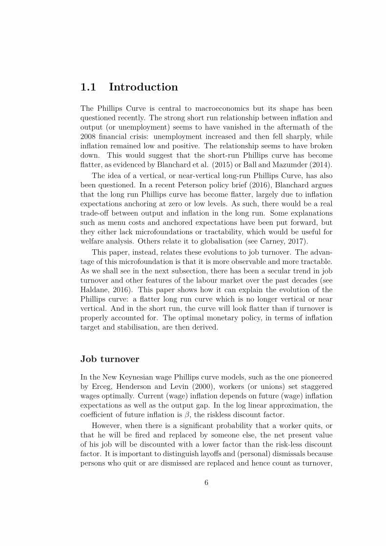
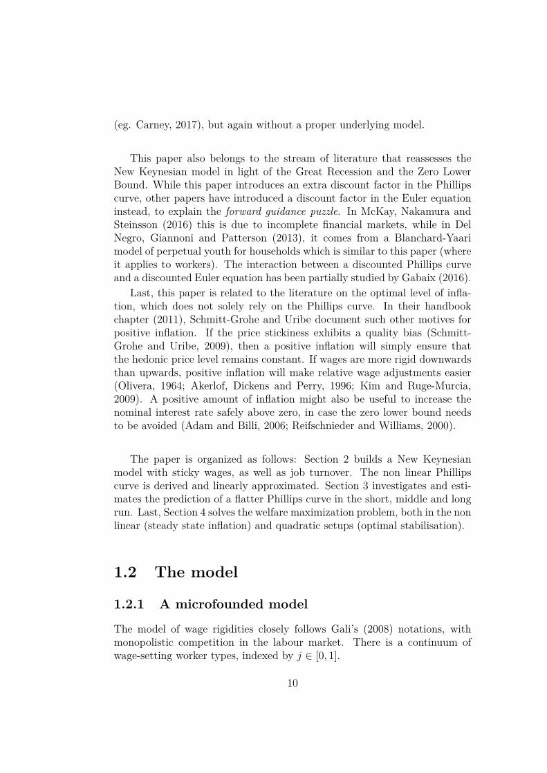
Figure 1.1 comes from the job tenure survey from the OECD, for peopleaged 25 − 54. The proportion of people less than a year into their job is agood indicator of yearly job turnover, though temporary contracts probablyoverstate the figure. In most countries, there has been an increase in the lessthan one year proportion of workers, which indicates a rising turnover. Thiscan also be seen with the increase of the less than three years proportion,which is less sensible to temporary employment. Last, the proportion ofpeople more than ten years into thir job has fallen accross most countries.This is highly suggestive of an increased turnover.

.05

.1.1

5.2

.25

turn

over

1990 1995 2000 2005 2010 2015Time

AUS BEL DNK DEU FINFRA ITA IRL NLD SWE

Figure 1.1: Turnover (OECD job tenure survey)

The increasing share of temporary contracts, and the recent rise in the1The probability of being laid off should not matter for the worker, if the union acts as

an insurance mechanism. Because the union is assumed to split the wage income betweenemployed and unemployed members, the employee does not lose his income when he islaid off. But turnover relates to quits and personal dismissals, not layoffs. And it is notthe purpose of the union to insure against these, so the turnover probability is a relevantdiscount factor.

7

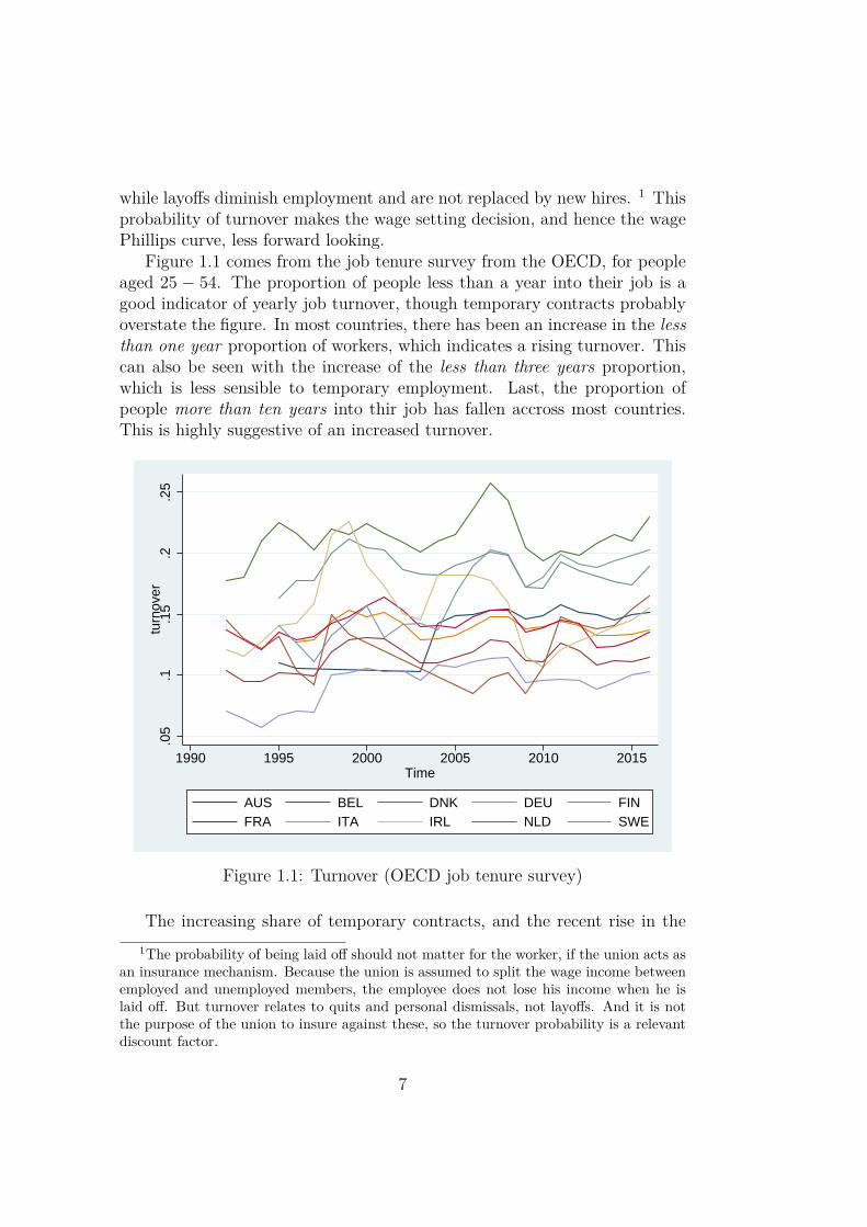
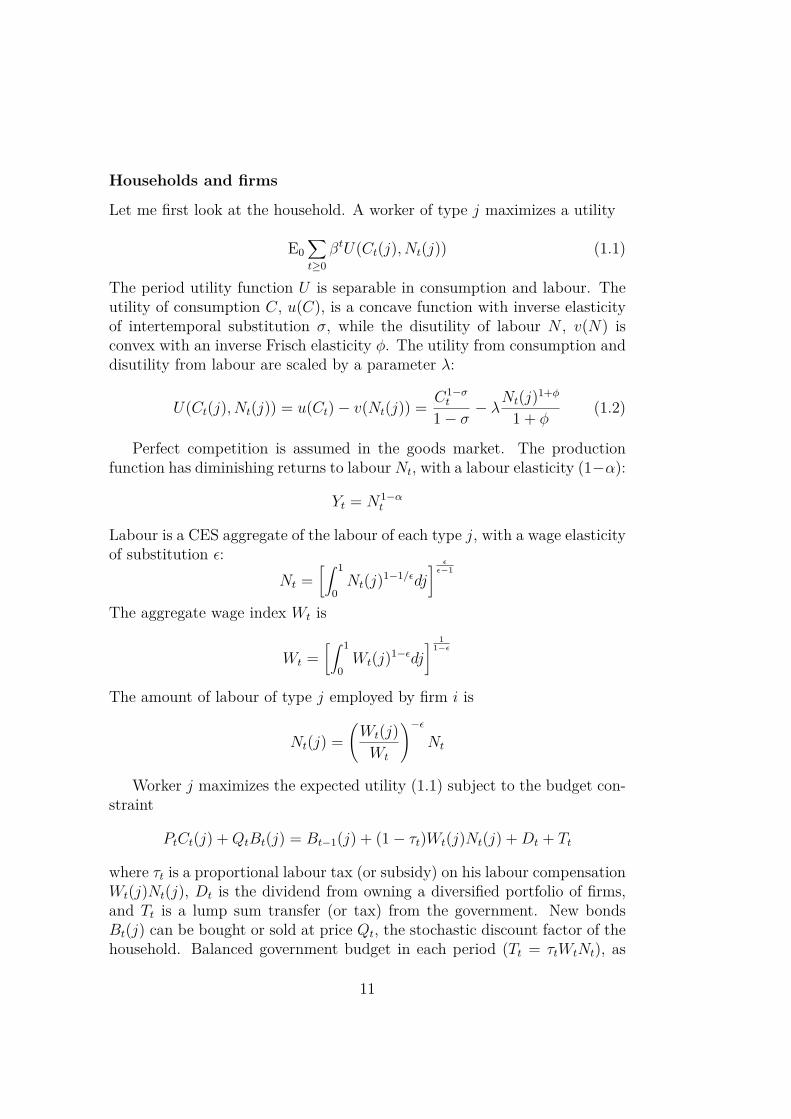
“gig economy”(part time contracts, self-employed contractors, zero-hours inBritain) are also likely to weaken collective bargaining in favour of moreindividual bargaining, as suggested by Haldane (2017). This would suggestlower wages, but also less forward looking decisions, which is the point of thispaper. Table 1.2 shows how the share of temporary contracts has evolvedover time (again using OECD data). While the upward trend is not alwaysmonotonic and varies in magnitude accross countries, it is relatively strong,especially in countries like France, Italy or the Netherlands).

05

1015

tem

pora

ry e

mpl

oym

ent (

%)

1980 1990 2000 2010 2020time

AUT BEL DNK DEU FINFRA ITA IRL NLD SWE

Figure 1.2: Share of temporary employment (OECD)

Calvo meets perpetual youthA crucial assumption is that when a worker quits (or is dismissed) and isreplaced by an entrant worker, the wage stickiness will be (at least partially)transmitted to the entrant. The entrant does not renegotiate its wage im-mediately, and has to abide by the wage of the previous incumbent it hasreplaced. Or equivalently, there is no difference between incumbents and en-trants in their distribution of wages. Assuming wage rigidity for new hires iscrucial in models such as Hall (2005) or Gertler and Trigari (2009), who com-bine wage and labour search frictions. Gertler, Huckfeldt and Trigari (2016)

8

find no evidence that the wage of new hires is more cyclical than for existingworkers. Galuscak et al. (2012) find similar results for 15 EU countries.

This model of entry has some perpetual youth flavour as in Blanchard(1985). As hinted by Weil (1989), the crucial feature in these models is asmuch the probability of death of the agent, as the stream of newborns, whodon’t have a say over decisions made before their birth. 2 Here, when a newworker starts a job, he is bound by the decisions of his predecessor. 3 Theexternality between existing and new agents creates the extra discounting.

Related literatureSnower and Tesfaselassie (2017) derive a positive optimal long run inflationtarget in the presence of job turnover, but they do not investigate the shortrun properties much. Bilbiie, Ghironi and Melitz (2012; 2016) as well asBilbiie, Fujiwara and Ghironi (2014) look at the optimal long run monetarypolicy in similar setup: sticky prices with firm entry and exit. In theirmodel, the exit probability affects the Phillips curve and the optimal longrun Ramsey policy. While these papers use a Rotemberg instead of a Calvoframework, and inflation offsets different long run distortions, the intuition,as well as the assumption that new workers cannot reset their wage, is largelythe same 4. But this paper shows how turnover leads to a flatter long runPhillips curve, and a perceived flatter curve in the short run. It also explainshow the optimality of price targeting is broken, compared to the classicalresult in Woodford (2003), Benigno and Woodford (2004), or Gali (2008).Last, it shows how optimal short run policies are affected.

Different explanations have been put forward for the recently flatterPhillips Curve. Ball and Mazumder (2011) suggest that with menu costs,price changes will be less frequent when inflation is low, and the resultingPhillips Curve will be flatter. Blanchard (2016) relies on anchored inflationexpectations. My approach has the advantage of tractability and observablemicro-foundations, which allow for a welfare analysis. While the labour mar-ket has been highlighted as a possible driver of the flatter Phillips Curve (seeHaldane, 2017 or chapter 2 of the October 2017 World Economic Outlook),no proper model has been suggested yet. The idea of a global Phillips Curve– inflation reacting to global not domestic conditions – has also been floated

2In the positive sense, the death probability creates the lower discount factor, but inthe normative sense, the externality is caused by the stream of new workers.

3Or if wages are set by a union, it only cares about the welfare of its existing members.4In my Calvo framework, workers adopt the wage distribution of existing workers. In

a Rotemberg setup, it is assumed that new workers (or firms) take the existing symmetricwage (or price), and are not free to choose their starting wage (price) optimally

9

(eg. Carney, 2017), but again without a proper underlying model.

This paper also belongs to the stream of literature that reassesses theNew Keynesian model in light of the Great Recession and the Zero LowerBound. While this paper introduces an extra discount factor in the Phillipscurve, other papers have introduced a discount factor in the Euler equationinstead, to explain the forward guidance puzzle. In McKay, Nakamura andSteinsson (2016) this is due to incomplete financial markets, while in DelNegro, Giannoni and Patterson (2013), it comes from a Blanchard-Yaarimodel of perpetual youth for households which is similar to this paper (whereit applies to workers). The interaction between a discounted Phillips curveand a discounted Euler equation has been partially studied by Gabaix (2016).

Last, this paper is related to the literature on the optimal level of infla-tion, which does not solely rely on the Phillips curve. In their handbookchapter (2011), Schmitt-Grohe and Uribe document such other motives forpositive inflation. If the price stickiness exhibits a quality bias (Schmitt-Grohe and Uribe, 2009), then a positive inflation will simply ensure thatthe hedonic price level remains constant. If wages are more rigid downwardsthan upwards, positive inflation will make relative wage adjustments easier(Olivera, 1964; Akerlof, Dickens and Perry, 1996; Kim and Ruge-Murcia,2009). A positive amount of inflation might also be useful to increase thenominal interest rate safely above zero, in case the zero lower bound needsto be avoided (Adam and Billi, 2006; Reifschnieder and Williams, 2000).

The paper is organized as follows: Section 2 builds a New Keynesianmodel with sticky wages, as well as job turnover. The non linear Phillipscurve is derived and linearly approximated. Section 3 investigates and esti-mates the prediction of a flatter Phillips curve in the short, middle and longrun. Last, Section 4 solves the welfare maximization problem, both in the nonlinear (steady state inflation) and quadratic setups (optimal stabilisation).

1.2 The model

1.2.1 A microfounded model

The model of wage rigidities closely follows Gali’s (2008) notations, withmonopolistic competition in the labour market. There is a continuum ofwage-setting worker types, indexed by j ∈ [0, 1].

10

Households and firms

Let me first look at the household. A worker of type j maximizes a utility

E0∑t≥0

βtU(Ct(j), Nt(j)) (1.1)

The period utility function U is separable in consumption and labour. Theutility of consumption C, u(C), is a concave function with inverse elasticityof intertemporal substitution σ, while the disutility of labour N , v(N) isconvex with an inverse Frisch elasticity φ. The utility from consumption anddisutility from labour are scaled by a parameter λ:

U(Ct(j), Nt(j)) = u(Ct)− v(Nt(j)) = C1−σt

1− σ − λNt(j)1+φ

1 + φ(1.2)

Perfect competition is assumed in the goods market. The productionfunction has diminishing returns to labour Nt, with a labour elasticity (1−α):

Yt = N1−αt

Labour is a CES aggregate of the labour of each type j, with a wage elasticityof substitution ε:

Nt =[∫ 1

0Nt(j)1−1/εdj

] εε−1

The aggregate wage index Wt is

Wt =[∫ 1

0Wt(j)1−εdj

] 11−ε

The amount of labour of type j employed by firm i is

Nt(j) =(Wt(j)Wt

)−εNt

Worker j maximizes the expected utility (1.1) subject to the budget con-straint

PtCt(j) +QtBt(j) = Bt−1(j) + (1− τt)Wt(j)Nt(j) +Dt + Tt

where τt is a proportional labour tax (or subsidy) on his labour compensationWt(j)Nt(j), Dt is the dividend from owning a diversified portfolio of firms,and Tt is a lump sum transfer (or tax) from the government. New bondsBt(j) can be bought or sold at price Qt, the stochastic discount factor of thehousehold. Balanced government budget in each period (Tt = τtWtNt), as

11

well as zero net supply of bonds, ensures that consumption and output areequal in each period:

PtCt = WtNt +Dt = PtYt

With perfect competition for goods, prices are equal to marginal costs, or

Pt = MCt = WtNαt

1− α

Hence the real wage is linked to output as

Ωt = (1− α)Y −α

1−αt

With decreasing returns to scale, firms make a profit Dt = αPtYt.

As in Erceg et al. (2000) or Gali (2008), let us assume markets withcomplete contingent claims for consumption but not leisure. This ensuresfull consumption smoothing accross agents.

Lemma 1. With complete markets, there is full consumption smoothing:

∀(t, j), Ct(j) = Ct = Yt

The Euler equation of consumption pins down the riskless discount factor

Qt = EtβPtPt+1

u′(Ct+1)u′(Ct)

= βPtPt+1

(Ct+1

Ct

)−σ(1.3)

The labour supply decision for a worker j in problem (1.1) is equivalent tomaximizing the following quantity in each period

u′(Yt)(1− τ)Wt(j)Nt(j)

Pt− λNt(j)1+φ

1 + φ(1.4)

Distortions and dispersions

Let us define the first-best and flexible outcomes. Using the utility andproduction function, the first-best level of output is

Y =(1− α

λ

) 1σ+φ+α

1−α

12

Lemma 2. In the flexible outcome, the real wage Ω = WP

is a markup µabove the marginal rate of substitution of the worker:

µ =(

ε

(ε− 1) (1− τ)

)

The flexible-wage output is

Y =(

1− αλµ

) 1σ+φ+α

1−α = Y

(1µ

) 1σ+φ+α

1−α

The markups depend on the wage elasticity – with a high elasticity, themarkup is close to 1. But it also depends on the wage tax τ . A positive taxcreates an additional wedge, but a subsidy can offset the inefficiency causedby the finite wage elasticity. Unless the subsidies fully offset the wedges(µ = 1), the flexible output will be inefficiently low as Y < Y .

With staggered wages, the wage dispersion will be costly in terms ofwelfare. When wages are heterogeneous, the aggregate number of hoursmust increase to produce the same amount of goods.

Lemma 3. The aggregate utility function can be written

∫ 1

0U(Ct, Nt(j))dj = Y 1−σ

(YtY

)1−σ

1− σ −1−α1+φ∆t

(YtY

) 1+φ1−α

µ

(1.5)

with the wage dispersions

∆t =∫ 1

0

(Wt(j)Wt

)−ε(1+φ)

dj ≥ 1 (1.6)

1.2.2 Sticky wages and the Phillips CurveWorker discounting

A fraction θ of workers have sticky wages, and a fraction δ keeps their jobfrom one period to another; the two are independent. The discount factoraccounts for the price and the firms survival probabilities θ and δ. Insteadof maximizing the discounted sum of expression (1.4) with a discount factorβ, the applicable rate of time preference will be βθδ: the disutility of labour– attached to a wage and a worker – is discounted by βθδ, while the labourcompensation is discounted by θδQt.

13

It is assumed that when a worker is replaced, the new worker cannotautomatically renegotiate his wage. Instead, he faces the same probability ofsticky wages than existing workers. If they were completely free to choose newwages, the effect would die out; but as long as the new wage partly takes intoaccount the wage of existing workers, the effect would be lessened but not dieout. This gives a discrepancy between the joint survival probability θδ of theoptimal wage setting decision, and the true wage stickiness θ that is featuredin the dynamics of the aggregate wage and dispersion. This is the cause ofthe flatter wage Phillips curve5. As mentioned before, evidence in Gertler etal. (2016) or Galuscak et al (2012) tends to support this assumption.

It is also possible to think about the case where it is the union whichsets the wage of workers of type j, and the union insures workers againstlayoffs but not quits or dismissals. When a worker quits, or is dismissed, wecan assume that he leaves his labour type and finds a different occupation,where wages are set by a different union. As such, if the union maximizesthe utility of its existing members, employed or not, it will have a shortdiscounting horizon. And it will not take into account the utility of futuremembers, because they do not belong to this union yet.

The non linear Phillips curve

When a worker is free to set a wage wt(j), he seeks to maximize the discountedsum of the wage compensation minus the disutility, defined in expression(1.4).

Et

∑(θβδ)T−t

[u′(YT )(1− τT )wt(j)NT (j)

PT− λNT (j)1+φ

1 + φ

]

Lemma 4. The re-optimizing price w∗t is :

(w∗tWt

)1+φε=

Et∑(θβδ)T−tµt

(Wt

WT

)−ε(1+φ)λN1+φ

T

Et∑(θβδ)T−t

(Wt

WT

)1−εΩTu′(YT )NT

=(Kt

Ft

)(1.7)

with recursive terms Ft and Kt

Ft = (1− α)Y 1−σt + θβδEtFt+1Πε−1

t+1 (1.8)

Kt = µtλY1+φ1−αt + θβδEtKt+1Πt+1

ε(1+φ) (1.9)5. In their Rotemberg setup, Snower and Tesfaselassie (2017) (or Bilbiie Ghironi and

Melitz, 2012;2016) assume that new workers (or firms) start with the symmetric wage(price) of existing workers (firms). It is similar to here: entrants are bound by incumbents

14

This is where the job survival probability, δ plays a role, compared tothe standard model. δ is an extra factor, appearing here in the worker’sdiscounting, through the recursive Ft and Kt. In the recursive equation, Ftdepends on the expected future value EtFt+1, multiplied by the inflation anda discount factor θβδ. The exact same phenomenon occurs for the recursiveterm Kt. The δ makes these two terms less forward looking than in thestandard model, and it makes the wage Phillips curve flatter, as we will seewith the linear approximation.

In each period, only a fraction (1 − θ) of wages are re-optimized at thevalue w∗t , while a fraction θ still follows the previous distribution of wages,with an aggregate Wt−1.Using the definition of the aggregate wage, the wagelevel Wt is a weighted aggregate of the previous wage level Wt−1 and thecurrent optimal wage w∗t : 6

W 1−εt = θW 1−ε

t−1 + (1− θ)(w∗t )1−ε

This provides the dynamics for the wage inflation and dispersion

1− θΠtε−1

1− θ = w(Πt) =(w∗tWt

)1−ε=(FtKt

) ε−11+φε

(1.10)

∆t = θ∆t−1Πtε(1+φ) + (1− θ)w(Πt)

ε(1+φ)ε−1 (1.11)

Linear quadratic setup

Although we will look at the optimal steady state level of inflation that thenon linear model yields, it is useful to derive a linear quadratic approximationaround a zero inflation steady state. In the flexible price steady state, thereis no inflation (Π = 1), and no dispersion (∆ = 1). The steady state valuesY , Ω, F and K are easy to pin down. Let us define the percentage deviationof each variable: πt = log Πt, and dt = log ∆t. Similarly yt, ωt, ft and ktdenote log deviations of the capital-letter variables from the steady state.

Proposition 1. The linear wage Phillips curve is

πt = κyt + βδEt [πt+1] (1.12)

with κ =(φ+α1−α + σ

)(1−θ)(1−θβδ)

θ1

1+φε

This linear wage Phillips curve is broadly similar with the standard wagePhillips curve in a model of price and wage stickiness. Current wage inflation

6Importantly, the new hires follow existing wages, so that turnover δ doesn’t play arole in this law of motion of the aggregate wage

15

positively depends on the output gap and future expected wage inflation,and negatively on the real wage. However, two differences stand out. Thecoefficient κ is slightly different as it features the parameter δ. But mostimportantly, future inflation is discounted by βδ instead of simply β. In termsof intuition, this is because βδ is now the discount factor that is applicableto the job tenure of the worker.

1.3 A flatter Phillips curve

1.3.1 Predictions of the modelNon vertical long run Phillips curve

The long run version of (1.12) implies a flatter long-run Phillips curves, andit is no longer vertical or nearly vertical as without turnover:

π = κ

1− βδ Y

When δ is smaller than 1, κ increases slightly. However the increasing effecton the denominator (1 − βδ) largely dominates. This means that long runinflation will depend less strongly on the long run output gap, and the curveis not as vertical.

Property 1. In the long run Phillips curve between inflation and output ofthe form π = χY , the coefficient χ decreases with turnover ( δ falls):

χ =(φ+ α

1− α + σ

)(1− θ)θ(1 + φε)

1− θβδ1− βδ

Because the linear equation is only an approximation of a highly non-linear model, it is useful to see the impact of turnover on the non linearlong run Phillips Curve. In steady state the price and wage inflation mustbe equalized: Π = Π. Taking the steady state in equations (1.8), (1.9) and(1.10), output can be written in terms of inflation

Lemma 5. The non linear long-run Phillips curve is

(Y

Y

)φ+α1−α+σ

=[

1− θβδΠε(1+φ)

1− θβδΠε−1 w(Π)−1+φεε−1

](1.13)

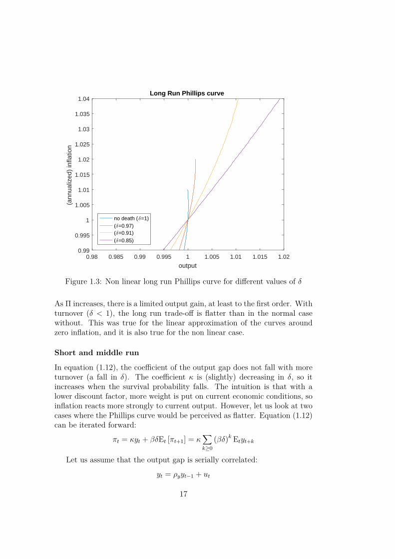
Figure (1.3) displays the output level Y associated to a long run (annual-ized, price and wage) inflation Π. When Π = 1, Y = 1 (the flex price case).

16

0.98 0.985 0.99 0.995 1 1.005 1.01 1.015 1.02

output

0.99

0.995

1

1.005

1.01

1.015

1.02

1.025

1.03

1.035

1.04

(ann

ualiz

ed)

infla

tion

Long Run Phillips curve

no death (δ=1)(δ=0.97)(δ=0.91)(δ=0.85)

Figure 1.3: Non linear long run Phillips curve for different values of δ

As Π increases, there is a limited output gain, at least to the first order. Withturnover (δ < 1), the long run trade-off is flatter than in the normal casewithout. This was true for the linear approximation of the curves aroundzero inflation, and it is also true for the non linear case.

Short and middle run

In equation (1.12), the coefficient of the output gap does not fall with moreturnover (a fall in δ). The coefficient κ is (slightly) decreasing in δ, so itincreases when the survival probability falls. The intuition is that with alower discount factor, more weight is put on current economic conditions, soinflation reacts more strongly to current output. However, let us look at twocases where the Phillips curve would be perceived as flatter. Equation (1.12)can be iterated forward:

πt = κyt + βδEt [πt+1] = κ∑k≥0

(βδ)k Etyt+k

Let us assume that the output gap is serially correlated:

yt = ρyyt−1 + ut

17

with ut a mean-zero disturbance. Then we can write inflation as

πt = κ

(1− ρyβδ)yt

Property 2. The slope of a traditional Phillips Curve displaying only currentinflation and output, πt = κyt , will depend on the ratio

(1− θβδ)(1− ρyβδ)

As long as ρy > θ (the output gap being more persistent than wages), theslope will decrease when δ falls (turnover increases).

Let us also look at an estimated New Keynesian Phillips curve with arestricted β, if the turnover is not accounted for. Using the assumptionsabove,

πt − βEt [πt+1] = κyt − β(1− δ)Et [πt+1]

πt − βEt [πt+1] = κ

yt − β(1− δ)∑k≥1

(βδ)k Etyt+k

Property 3. The estimated slope in this case will be

κ∗ = cov(πt − βEt [πt+1] , yt)var(yt)

= (1− βρy)(1− ρyβδ)

κ

As long as ρy > θ (the output gap being more persistent than wages), theslope will decrease when δ falls (turnover increases).

This is the case in the empirical estimates of Gali and Gertler (1999),where they use marginal costs instead of the output gap. They estimateπt = λmct +βEπt+1. The estimated coefficient of marginal costs, λ, dependson the assumption about the coefficient of future inflation, β. When thiscoefficient is restricted to β = 1, the estimated value of λ is smaller thanwhen there is no restriction and β.takes a lower value.

Remark We have to assume here that the output gap is more persistentthan sticky wages (ρy > θ) in order to generate a downward bias in thetraditional PC, and the restricted New Keynesian PC. This is not difficultas ρy ≈ 0.95 in the US for example. However, such an assumption would notbe necessary in a Rotemberg setup. In such a setup, the coefficient κ doesnot depend on turnover. Assuming yt = ρyyt−1 + ut as before, (1− ρyβδ)increases when δ falls, so the traditional and restricted New Keynesian slopesare always smaller with turnover.

18

1.3.2 Empirical resultsI rely on data from the OECD to test a wage Phillips curve between inflationand cyclical unemployment7. I have 21 countries, between 1996 and 2014(or fewer years for some countries). Cyclical unemployment ut is definedas unemployment minus the NAIRU, or structural unemployment. Wagegrowth is the yearly percentage increase in nominal compensation per worker.For turnover, I rely on the job tenure survey. While the proportion of workerwho have been in their job for less than a year is not a perfect metrics forthe rate of yearly job turnover, it is nevertheless a relatively good indicator.Therefore my turnover variable τt is the proportion of worker between 25 and54 who have been in their job for a year or less.

I run two regressions.8 The first is a short run expectation-based curve:

πt = γ(τt)ut + β(τt)πt+1 + vt

where vt is an error term. γ(τt) is expected to be negative, and decreaseslightly with turnover τt (a slightly steeper curve). β(τt) is positive andsmaller than 1, and it should decrease with τt. In order to test the effect ofturnover on these coefficients, I add the cross terms (τt × ut) and (τt × πt+1)in the regression. The two estimates are expected to be negative. I also addtime and country fixed effects in the regression. Last, to rule out commontrends in turnover and the coefficients, I also allow a trend in the coefficients.As such, the equation can be written

πn,t = αn + αt + γ1un,t + γ2(τn,t × un,t) + γ3(t× un,t)+βπn,t+1 + β2(τn,t × πn,t+1) + β3(t× πn,t+1) + vn,t

The results are coherent with the predictions of the model. The effect ofturnover on the coefficient of future inflation is negative and significant, aspredicted. And allowing for a trend in the coefficient does not make turnoverinsignificant. Contrary to the prediction, the unemployment coefficient in-creases with turnover (which makes the curve flatter). But this effect waspredicted to be small, and in the data the change is positive but insignificant.The flatter unemployment coefficient might be caused by less frequent wagechanges as in the menu costs model of Ball and Mazumder (2011): changes

7It as long been argued (see, eg. Gali and Gertler, 1999; or Gali, 2011) that Phillipscurve are easier to estimate with real marginal costs or unemployment than with output

8Consistency of my OLS approach requires that unemployment and turnover are ex-ogenous. In particular, they cannot be correlated with any lead or lag of the error termvt – which also captures variations of the desired wage markup. If there is such a correla-tion, OLS would be inconsistent, and models such as VAR or GMM could control for theendogeneity issue.

19

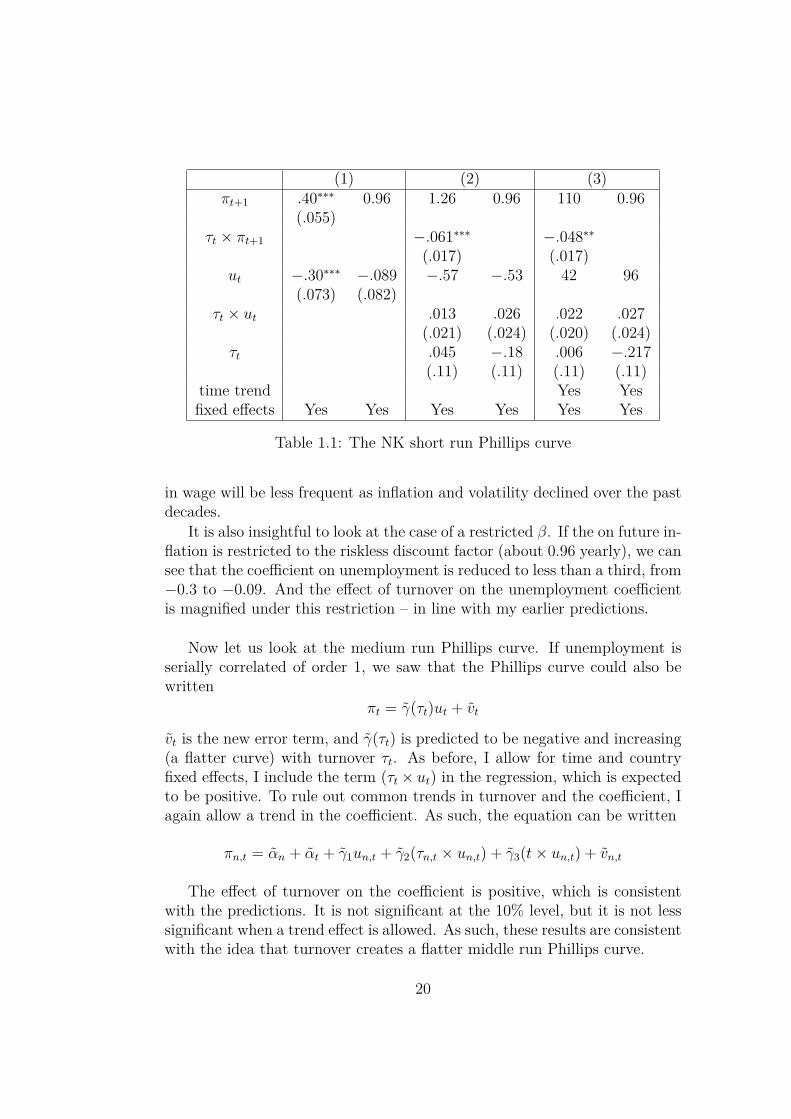
(1) (2) (3)πt+1 .40∗∗∗ 0.96 1.26 0.96 110 0.96

(.055)τt × πt+1 −.061∗∗∗ −.048∗∗

(.017) (.017)ut −.30∗∗∗ −.089 −.57 −.53 42 96

(.073) (.082)τt × ut .013 .026 .022 .027

(.021) (.024) (.020) (.024)τt .045 −.18 .006 −.217

(.11) (.11) (.11) (.11)time trend Yes Yesfixed effects Yes Yes Yes Yes Yes Yes

Table 1.1: The NK short run Phillips curve

in wage will be less frequent as inflation and volatility declined over the pastdecades.

It is also insightful to look at the case of a restricted β. If the on future in-flation is restricted to the riskless discount factor (about 0.96 yearly), we cansee that the coefficient on unemployment is reduced to less than a third, from−0.3 to −0.09. And the effect of turnover on the unemployment coefficientis magnified under this restriction – in line with my earlier predictions.

Now let us look at the medium run Phillips curve. If unemployment isserially correlated of order 1, we saw that the Phillips curve could also bewritten

πt = γ(τt)ut + vt

vt is the new error term, and γ(τt) is predicted to be negative and increasing(a flatter curve) with turnover τt. As before, I allow for time and countryfixed effects, I include the term (τt× ut) in the regression, which is expectedto be positive. To rule out common trends in turnover and the coefficient, Iagain allow a trend in the coefficient. As such, the equation can be written

πn,t = αn + αt + γ1un,t + γ2(τn,t × un,t) + γ3(t× un,t) + vn,t

The effect of turnover on the coefficient is positive, which is consistentwith the predictions. It is not significant at the 10% level, but it is not lesssignificant when a trend effect is allowed. As such, these results are consistentwith the idea that turnover creates a flatter middle run Phillips curve.

20

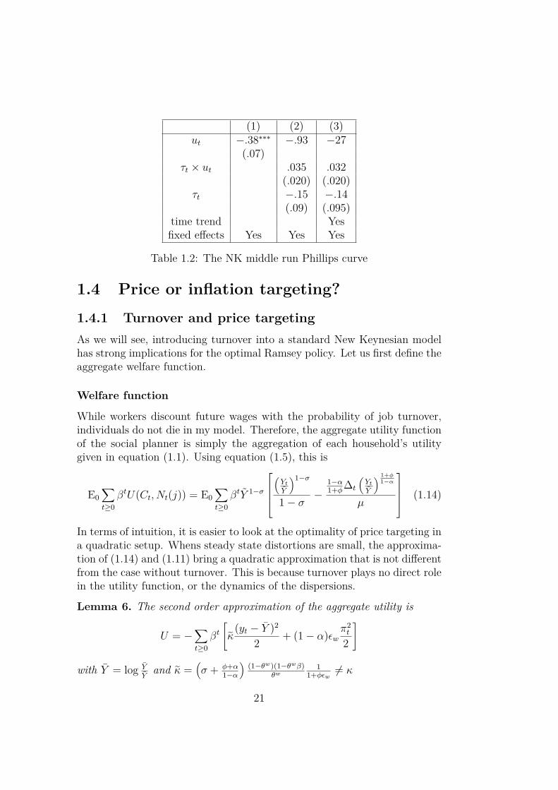
(1) (2) (3)ut −.38∗∗∗ −.93 −27

(.07)τt × ut .035 .032

(.020) (.020)τt −.15 −.14

(.09) (.095)time trend Yesfixed effects Yes Yes Yes

Table 1.2: The NK middle run Phillips curve

1.4 Price or inflation targeting?

1.4.1 Turnover and price targetingAs we will see, introducing turnover into a standard New Keynesian modelhas strong implications for the optimal Ramsey policy. Let us first define theaggregate welfare function.

Welfare function

While workers discount future wages with the probability of job turnover,individuals do not die in my model. Therefore, the aggregate utility functionof the social planner is simply the aggregation of each household’s utilitygiven in equation (1.1). Using equation (1.5), this is

E0∑t≥0

βtU(Ct, Nt(j)) = E0∑t≥0

βtY 1−σ

(YtY

)1−σ

1− σ −1−α1+φ∆t

(YtY

) 1+φ1−α

µ

(1.14)

In terms of intuition, it is easier to look at the optimality of price targeting ina quadratic setup. Whens steady state distortions are small, the approxima-tion of (1.14) and (1.11) bring a quadratic approximation that is not differentfrom the case without turnover. This is because turnover plays no direct rolein the utility function, or the dynamics of the dispersions.

Lemma 6. The second order approximation of the aggregate utility is

U = −∑t≥0

βt[κ

(yt − Y )2

2 + (1− α)εwπ2t

2

]

with Y = log YY

and κ =(σ + φ+α

1−α

)(1−θw)(1−θwβ)

θw1

1+φεw 6= κ

21

Contrary to κ, δ does not appear in κ, which is exactly the same coefficientas in the case with no turnover. This is because the distortion is discountedwith the discount factor of the household, where the death shocks play norole.

Let us also assume cost push shocks in the Phillips curve:

πt = κyt + βδEtπt+1 + ut

with ut the cost push shock, an error term. We allow it to be an AR(1)process with autocorrelation ρu (ρu = 0 denoting the white noise case).

The optimality of price targeting

Proposition 2. When δ = 1, price targeting is optimal for the Ramsey pol-icy: even with steady state distortions, the long run optimal level of inflationis zero; while inflation reacts to cost push shocks in the short run, this isaccompanied by deflation in the future, so that there is full mean reversion ofthe price level. In other words, there is long-run price targeting in responseboth to long term distortions and short term cost push shocks

When δ < 1, price targeting is no longer optimal: long run inflation isnon zero if there are steady state distortions; in response to cost push shocks,some deflation in the future offsets the initial response of inflation, but thereis no longer full mean reversion of the price level. In other words, pricetargeting does not hold anymore.

The intuition is as follows: in the benchmark, by committing to giveup some discretion in the future, the planner has some extra discretion inthe present correct cost push shocks, or an inefficient steady state. So thatprice stability is optimal from today’s perspective, but there is an incentive torenege tomorrow. With the death shock, firms are less responsive to commit-ments, so that the current gain in terms of commitment no longer offsets theinefficiency in the future. Thus, even with a credible commitment, inflationwill always be used to offset cost push shocks or steady state inefficiencies.

To better grasp the logic, it is useful to compare the Ramsey policy,which is history dependent, to an optimal state dependent policy. While sucha solution is not Ramsey optimal, it features no dynamic inconsistency. Wecan call this solutionMarkovian, or Recursively Pareto Optimal as in Brendonand Ellison (2015). Let us assume that the optimal inflation is a function ofthe first-best rate of output and the current cost push shock: πt = π + γπut.

In such a Markovian setup, the optimal inflation is not zero even withoutturnover. This is because the long run Phillips Curve is not vertical withoutturnover, and a very little amount of inflation is welfare improving. On

22

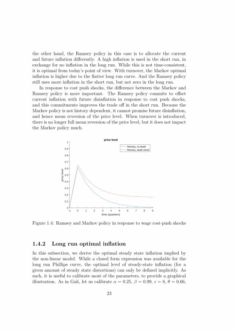
the other hand, the Ramsey policy in this case is to allocate the currentand future inflation differently. A high inflation is used in the short run, inexchange for no inflation in the long run. While this is not time-consistent,it is optimal from today’s point of view. With turnover, the Markov optimalinflation is higher due to the flatter long run curve. And the Ramsey policystill uses more inflation in the short run, but not zero in the long run.

In response to cost push shocks, the difference between the Markov andRamsey policy is more important. The Ramsey policy commits to offsetcurrent inflation with future disinflation in response to cost push shocks,and this commitments improves the trade off in the short run. Because theMarkov policy is not history dependent, it cannot promise future disinflation,and hence mean reversion of the price level. When turnover is introduced,there is no longer full mean reversion of the price level, but it does not impactthe Markov policy much.

-1 0 1 2 3 4 5 6 7 8 9

time (quarters)

0

0.1

0.2

0.3

0.4

0.5

0.6

0.7

0.8

0.9

1

pric

e le

vel

price level

Ramsey, no deathRamsey, death shock

Figure 1.4: Ramsey and Markov policy in response to wage cost-push shocks

1.4.2 Long run optimal inflationIn this subsection, we derive the optimal steady state inflation implied bythe non-linear model. While a closed form expression was available for thelong run Phillips curve, the optimal level of steady-state inflation (for agiven amount of steady state distortions) can only be defined implicitly. Assuch, it is useful to calibrate most of the parameters, to provide a graphicalillustration. As in Gali, let us calibrate α = 0.25, β = 0.99, ε = 8, θ = 0.66,

23

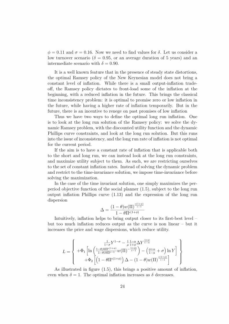
φ = 0.11 and σ = 0.16. Now we need to find values for δ. Let us consider alow turnover scenario (δ = 0.95, or an average duration of 5 years) and anintermediate scenario with δ = 0.90.

It is a well known feature that in the presence of steady state distortions,the optimal Ramsey policy of the New Keynesian model does not bring aconstant level of inflation. While there is a small output-inflation trade-off, the Ramsey policy dictates to front-load some of the inflation at thebeginning, with a reduced inflation in the future. This brings the classicaltime inconsistency problem: it is optimal to promise zero or low inflation inthe future, while having a higher rate of inflation temporarily. But in thefuture, there is an incentive to renege on past promises of low inflation

Thus we have two ways to define the optimal long run inflation. Oneis to look at the long run solution of the Ramsey policy: we solve the dy-namic Ramsey problem, with the discounted utility function and the dynamicPhillips curve constraints, and look at the long run solution. But this runsinto the issue of inconsistency, and the long run rate of inflation is not optimalfor the current period.

If the aim is to have a constant rate of inflation that is applicable bothto the short and long run, we can instead look at the long run constraints,and maximize utility subject to them. As such, we are restricting ourselvesto the set of constant inflation rates. Instead of solving the dynamic problemand restrict to the time-invariance solution, we impose time-invariance beforesolving the maximization.

In the case of the time invariant solution, one simply maximizes the per-period objective function of the social planner (1.5), subject to the long runoutput inflation Phillips curve (1.13) and the expression of the long rundispersion

∆ = (1− θ)w(Π)ε(1+φ)ε−1

1− θΠε(1+φ)

Intuitively, inflation helps to bring output closer to its first-best level –but too much inflation reduces output as the curve is non linear – but itincreases the price and wage dispersions, which reduce utility.

L =

11−σY

1−σ − 1µ

1−α1+φ∆Y

1+φ1−α

+Φ1

[ln(

1−θβδΠε(1+φ)

1−θβδΠε−1 w(Π)−1+φεε−1

)−(φ+α1−α + σ

)ln Y

]+Φ2

[(1− θΠε(1+φ)

)∆− (1− θ)w(Π)

ε(1+φ)ε−1

]

As illustrated in figure (1.5), this brings a positive amount of inflation,even when δ = 1. The optimal inflation increases as δ decreases.

24

For the timeless Ramsey policy, we write the full dynamic Lagrangian(with Yt, Ωt, Kt and Ft renormalized to flex price values).

The social planner maximizes the discounted sum of the per period util-ities (1.5), subject, in each period, to the recursive expressions of Ft and Kt

(equations 1.8 and 1.9), the ratio KtFt

(equation 1.10), as well as the dynamicsof ∆t (equations 1.11).

Intuitively the trade-offs are similar to the time invariant problem: in-flation increases output at the first order, but increases the costly price andwage distortions. However, the fully dynamic setting is different from thepreviously static one. The Lagrangian of the problem writes

L =∑

βt

[1

1−σY1−σt − 1

µt1−α1+φY

1+φ1−αt ∆t

]+φ1,t

[Ktw(Πt)

1+φεε−1 − Ft

]+φ2,t

[Ft − Y 1−σ

t − θβδEtFt+1Πε−1t+1

]+φ3,t

[Kt − Y

1+φ1−αt − θβδEtKt+1Πt+1

ε(1+φ)]

+φ4,t

[∆t − θ∆t−1Πt

ε(1+φ) − (1− θ)w(Πt)ε(1+φ)ε−1

]

After taking the first order conditions, we look at the steady state value

of each constraint and multiplier. Figure (1.5) displays the optimal rate ofinflation depending on the amount of steady state distortions, for differentvalues of δ. When δ = 1, we have the classic result of zero inflation in thelong run, but it increases as this parameter decreases.

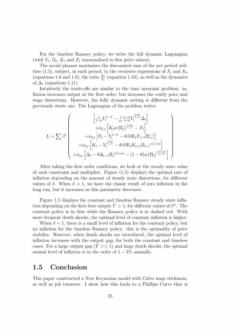
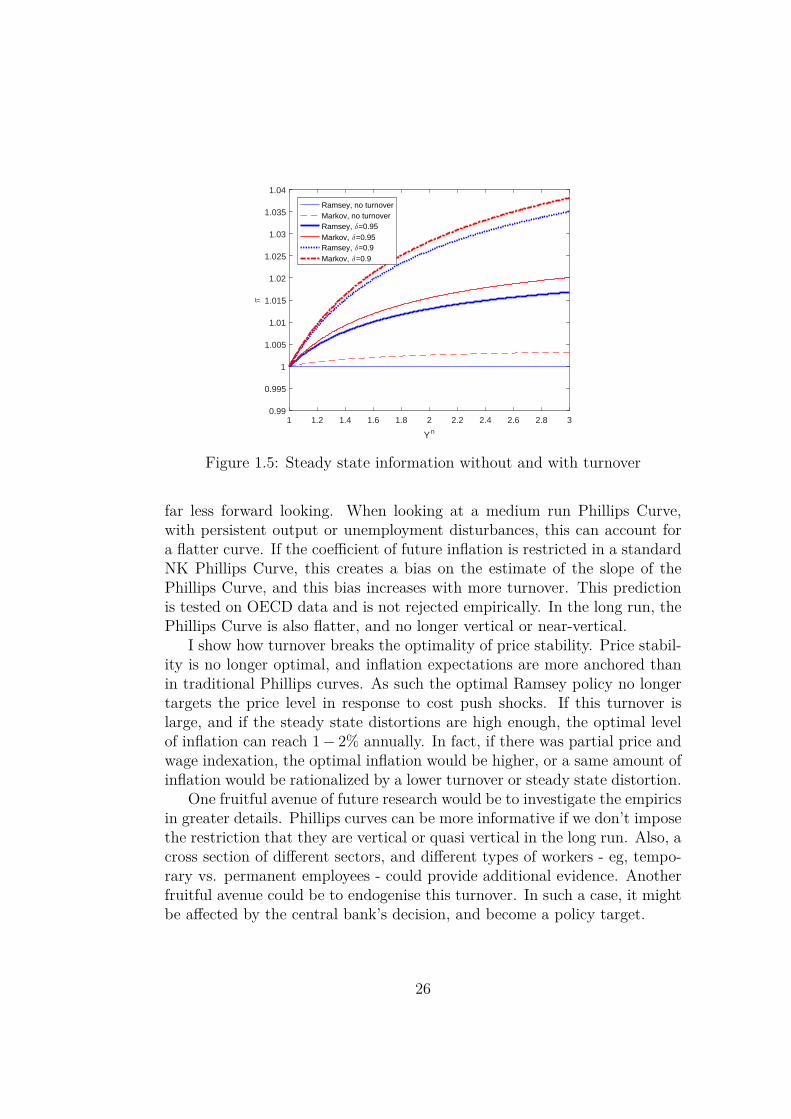
Figure 1.5 displays the constant and timeless Ramsey steady state infla-tion depending on the first-best output Y > 1, for different values of δw. Theconstant policy is in blue while the Ramsey policy is in dashed red. Withmore frequent death shocks, the optimal level of constant inflation is higher.

When δ = 1, there is a small level of inflation for the constant policy, butno inflation for the timeless Ramsey policy: this is the optimality of pricestability. However, when death shocks are introduced, the optimal level ofinflation increases with the output gap, for both the constant and timelesscases. For a large output gap (Y >> 1) and large death shocks, the optimalannual level of inflation is in the order of 1− 3% annually.

1.5 ConclusionThis paper constructed a New Keynesian model with Calvo wage stickiness,as well as job turnover. I show how this leads to a Phillips Curve that is

25

1 1.2 1.4 1.6 1.8 2 2.2 2.4 2.6 2.8 3

Yn

0.99

0.995

1

1.005

1.01

1.015

1.02

1.025

1.03

1.035

1.04

π

Ramsey, no turnoverMarkov, no turnoverRamsey, δ=0.95Markov, δ=0.95Ramsey, δ=0.9Markov, δ=0.9

Figure 1.5: Steady state information without and with turnover

far less forward looking. When looking at a medium run Phillips Curve,with persistent output or unemployment disturbances, this can account fora flatter curve. If the coefficient of future inflation is restricted in a standardNK Phillips Curve, this creates a bias on the estimate of the slope of thePhillips Curve, and this bias increases with more turnover. This predictionis tested on OECD data and is not rejected empirically. In the long run, thePhillips Curve is also flatter, and no longer vertical or near-vertical.

I show how turnover breaks the optimality of price stability. Price stabil-ity is no longer optimal, and inflation expectations are more anchored thanin traditional Phillips curves. As such the optimal Ramsey policy no longertargets the price level in response to cost push shocks. If this turnover islarge, and if the steady state distortions are high enough, the optimal levelof inflation can reach 1− 2% annually. In fact, if there was partial price andwage indexation, the optimal inflation would be higher, or a same amount ofinflation would be rationalized by a lower turnover or steady state distortion.

One fruitful avenue of future research would be to investigate the empiricsin greater details. Phillips curves can be more informative if we don’t imposethe restriction that they are vertical or quasi vertical in the long run. Also, across section of different sectors, and different types of workers - eg, tempo-rary vs. permanent employees - could provide additional evidence. Anotherfruitful avenue could be to endogenise this turnover. In such a case, it mightbe affected by the central bank’s decision, and become a policy target.

26

Chapter 2

Monopoly, Monopsony,and the Phillips Curve

27

2.1 IntroductionAfter the 2008 financial crisis, unemployment increased and then fell sharply,while inflation remained low and positive. The correlation between inflationand unemployment – the Phillips Curve – is not as strong empirically as itwas before. The Phillips Curve has become flatter, as evidenced by Blanchardet al. (2015) or Ball and Mazumder (2014).

Policymakers such as Haldane (2016), Kuroda (2017) or the IMF (WEO,Oct 2017) are hinting towards the labor market as a possible cause for this.The bargaining power of workers and unions has declined over time in mostcountries. As a result, their ability to obtain wage increases might be reduced.The gig economy, temporary employment, work agencies, and more generallythe increased bargaining power of employers, might be causes of the weakerlink between employment and wage inflation. It is however unclear whetherthe impact of these trends is permanent or temporary. To the extent that thiscan affect the real wage, are we simply observing a temporary lower nominalwage growth while the real wage slowly falls? Is this simply a temporarydeflationary pressure? Or does this gig economy have a more fundamentalimpact on inflation and the way we think monetary policy?

The interplay between structural reforms – in the goods and labour mar-ket – and monetary policy has also been debated in the Eurozone. At Sintrain 2015, ECB President Mario Draghi famously pushed for market reformsand flexibility as a complement to monetary policy: "Any reforms under-taken now will in fact have an improved interaction with macroeconomicstabilisation policies." Is there a role for structural policies to stabilize eco-nomic activity and inflation, alongside fiscal and monetary policy? Did theNew Deal’s "codes of fair competition" simply create inflationary pressure byraising prices and wages, or did the reduced competition interact with themonetary and fiscal expansions? Did market deregulation and the weakeningof unions and collective bargaining in the US and the UK in the 1980s playa role in their disinflation? By shifting power from workers to firms, did theGerman Hartz reforms change the German Phillips curve for good?

This paper argues that the rise in monopsony power – the bargainingpower of employers in the labour market – not only influences the limitedwage growth that has been observed recently, but also has a more profoundimpact on the Phillips Curve and on monetary policy.

28

Monopsony in the labour marketLiterally, monopsony is a market situation in which there is only one buyer,as opposed to monopoly with only one seller. More generally, it encompassesthe case of an individual buyer facing an elastic supply curve. This couldbe the result of a pure monopsony with only one buyer, or a limited numberof buyers (oligopsony). But modern theories of monopsony emphasize therole of other frictions in the market. In the same way that a one percentincrease in a firm’s price is unlikely to crowd out all consumption, a onepercent reduction in the wage it pays will not crowd all employment.

The candidates for monopsonistic frictions are the same as those for mo-nopolistic frictions. If workers cannot observe the wage offered by every firm,or if a supplier cannot observe the price paid by all downstream buyers, therewill be a search friction where it takes time, effort or money to find a newemployer or customer – in the same way that finding a new worker or suppliercan be costly in monopolistic models. In terms of mobility costs, the canoni-cal Salop or Hotelling model can be used for either monopoly or monopsony.But one can also assume that employers or buyers are differentiated alongmeaningful characteristics, so that they are imperfect substitutes.

Any market, goods or services, could be monopsonistic in theory. Inthe goods market, the most common examples are agriculture, mining andforestry. Cattle, corn, fruits, wood logs are very homogeneous commodities,used as intermediate inputs for food processing or manufacturing. While thecommodity is very homogeneous, with little room for product differentiation,and with a large number of small producers, food processing and manufactur-ing firms are much bigger and more differentiated, giving them more marketpower both for their output and input goods.

Traditionally, only a few labour markets were considered monopsonic.Nurses, policemen, teachers may have only one potential employer: the localor national government. Even with local governments, monopsony will bestrong if pay is decided at the national or regional level. Company townsof the Industrial Revolution were another example of monopsonic employers,providing employment, housing and amenities for the whole town.

But some labour economist have recently argued that monopsony is per-vasive in other employment markets. With the fall in unionization and col-lective bargaining, monopoly is losing relevance as a description of the labourmarket. The increase in self-employment, flexible and part-time work – theso called gig economy – has made work more divisible and insecure (Hal-dane 2017). This divisibility and insecurity is a likely further shift in marketpower from workers to employers, making monopsony even more relevant tounderstand the labour market.

29

Monopsony and the Phillips CurveThis paper formalizes the policymakers’ insight of a link between the gigeconomy and the Phillips Curve, by looking at the role that monopsonicemployers can have in the determination of wages and inflation. The NewKeynesian model usually assumes that wages are set by workers or unionshaving monopoly power. Individual workers face a labor demand curve thatis not perfectly elastic. Here, I relax the assumption that wages are set byemployees, and I look at the effect of employers setting wages for their em-ployees. Individual employers face a labor supply curve that is not perfectlyelastic: they have monopsony power.

In the normal wage Phillips Curve with monopoly power, wages are set byemployees (or unions) who face nominal rigidities. When there is inflation,the nominal wage cannot be fully adjusted. The real wage falls, and labourdemand – hence output – increases. This provides the positive correlationbetween inflation and output under the classical monopoly case.

But if wages are set by firms who face nominal rigidities, and there isinflation, firms cannot adjust their wages fully. The real wage falls, andlabour supply hence output decreases. This provides a Phillips Curve wherethe output gap is negatively correlated with wage inflation.

The same would be true in the goods market. If sticky prices are set byproducers, and there is inflation, the markup falls, and demand increases.But if sticky prices are set by monopsonic consumers (or, possibly, by largeretailers and supermarkets), then the supply of goods by producers will fallwhen inflation lowers the price compared to nominal costs.

This paper also studies the interplay of monopoly and monopsony powerin the same market: workers and firms both have limited market power to seta wage. Instead of one agent choosing the level of employment in response tothe wage set by the other agent, there is a two-stage process for determiningthe wage and employment, and there is Nash bargaining in the two stages.

The result is different from monopoly pricing, monopsony pricing or per-fect competition. As such it can be thought of the general case encompassingthese particular cases. This setup can be used to study a gradual shift inbargaining power from workers to firms. As the bargaining power of firmsincreases, the Phillips Curve flattens, up to a point when the slope is inverted.

30

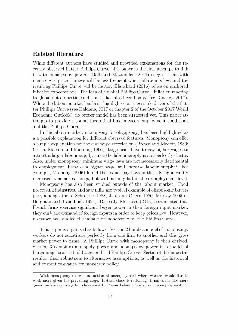
Related literatureWhile different authors have studied and provided explanations for the re-cently observed flatter Phillips Curve, this paper is the first attempt to linkit with monopsony power. Ball and Mazumder (2011) suggest that withmenu costs, price changes will be less frequent when inflation is low, and theresulting Phillips Curve will be flatter. Blanchard (2016) relies on anchoredinflation expectations. The idea of a global Phillips Curve – inflation reactingto global not domestic conditions – has also been floated (eg. Carney, 2017).While the labour market has been highlighted as a possible driver of the flat-ter Phillips Curve (see Haldane, 2017 or chapter 2 of the October 2017 WorldEconomic Outlook), no proper model has been suggested yet. This paper at-tempts to provide a sound theoretical link between employment conditionsand the Phillips Curve.

In the labour market, monopsony (or oligopsony) has been highlighted asa a possible explanation for different observed features. Monopsony can offera simple explanation for the size-wage correlation (Brown and Medoff, 1989;Green, Machin and Manning 1996): large firms have to pay higher wages toattract a larger labour supply, since the labour supply is not perfectly elastic.Also, under monopsony, minimum wage laws are not necessarily detrimentalto employment, because a higher wage will increase labour supply.1 Forexample, Manning (1996) found that equal pay laws in the UK significantlyincreased women’s earnings, but without any fall in their employment level.

Monopsony has also been studied outside of the labour market. Foodprocessing industries, and saw mills are typical example of oligopsonic buyers(see, among others, Schroeter 1988, Just and Chern 1980, Murray 1995 orBergman and Brännlund, 1995). Recently, Morlacco (2018) documented thatFrench firms exercise significant buyer power in their foreign input market:they curb the demand of foreign inputs in order to keep prices low. However,no paper has studied the impact of monopsony on the Phillips Curve.

This paper is organised as follows. Section 2 builds a model of monopsony:workers do not substitute perfectly from one firm to another and this givesmarket power to firms. A Phillips Curve with monopsony is then derived.Section 3 combines monopoly power and monopsony power in a model ofbargaining, so as to build a generalised Phillips Curve. Section 4 discusses theresults: their robustness to alternative assumptions, as well as the historicaland current relevance for monetary policy.

1With monopsony there is no notion of unemployment where workers would like towork more given the prevailing wage. Instead there is rationing: firms could hire moregiven the low real wage but choose not to. Nevertheless it leads to underemployment.

31

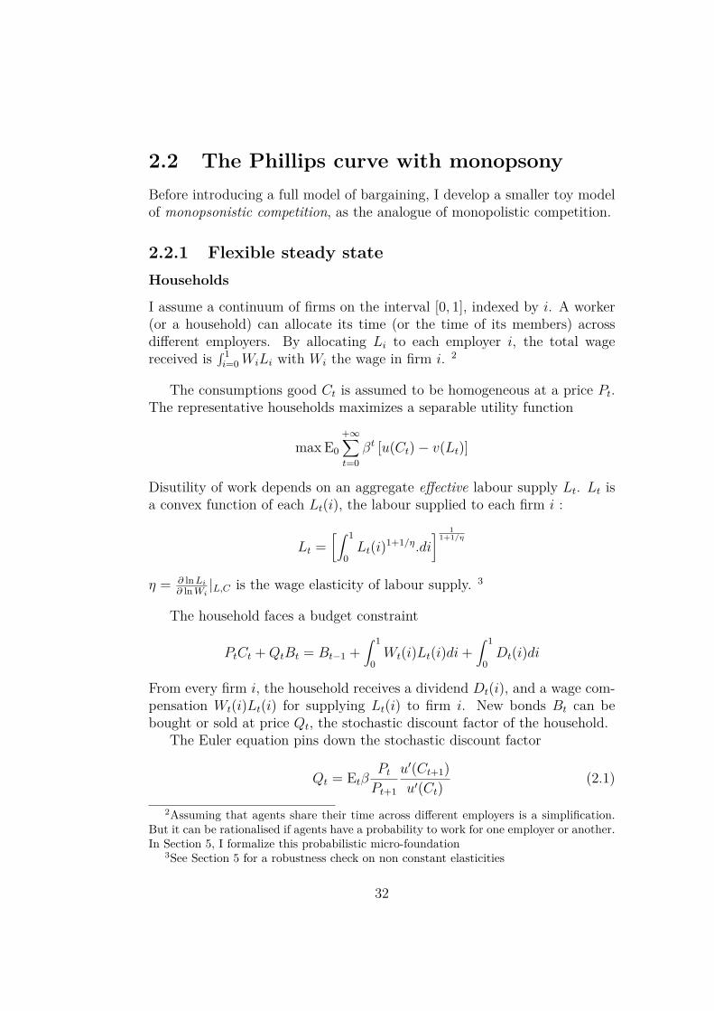
2.2 The Phillips curve with monopsonyBefore introducing a full model of bargaining, I develop a smaller toy modelof monopsonistic competition, as the analogue of monopolistic competition.

2.2.1 Flexible steady stateHouseholds

I assume a continuum of firms on the interval [0, 1], indexed by i. A worker(or a household) can allocate its time (or the time of its members) acrossdifferent employers. By allocating Li to each employer i, the total wagereceived is

∫ 1i=0WiLi with Wi the wage in firm i. 2

The consumptions good Ct is assumed to be homogeneous at a price Pt.The representative households maximizes a separable utility function

max E0

+∞∑t=0

βt [u(Ct)− v(Lt)]

Disutility of work depends on an aggregate effective labour supply Lt. Lt isa convex function of each Lt(i), the labour supplied to each firm i :

Lt =[∫ 1

0Lt(i)1+1/η.di

] 11+1/η

η = ∂ lnLi∂ lnWi

|L,C is the wage elasticity of labour supply. 3

The household faces a budget constraint

PtCt +QtBt = Bt−1 +∫ 1

0Wt(i)Lt(i)di+

∫ 1

0Dt(i)di

From every firm i, the household receives a dividend Dt(i), and a wage com-pensation Wt(i)Lt(i) for supplying Lt(i) to firm i. New bonds Bt can bebought or sold at price Qt, the stochastic discount factor of the household.

The Euler equation pins down the stochastic discount factor

Qt = EtβPtPt+1

u′(Ct+1)u′(Ct)

(2.1)

2Assuming that agents share their time across different employers is a simplification.But it can be rationalised if agents have a probability to work for one employer or another.In Section 5, I formalize this probabilistic micro-foundation

3See Section 5 for a robustness check on non constant elasticities

32

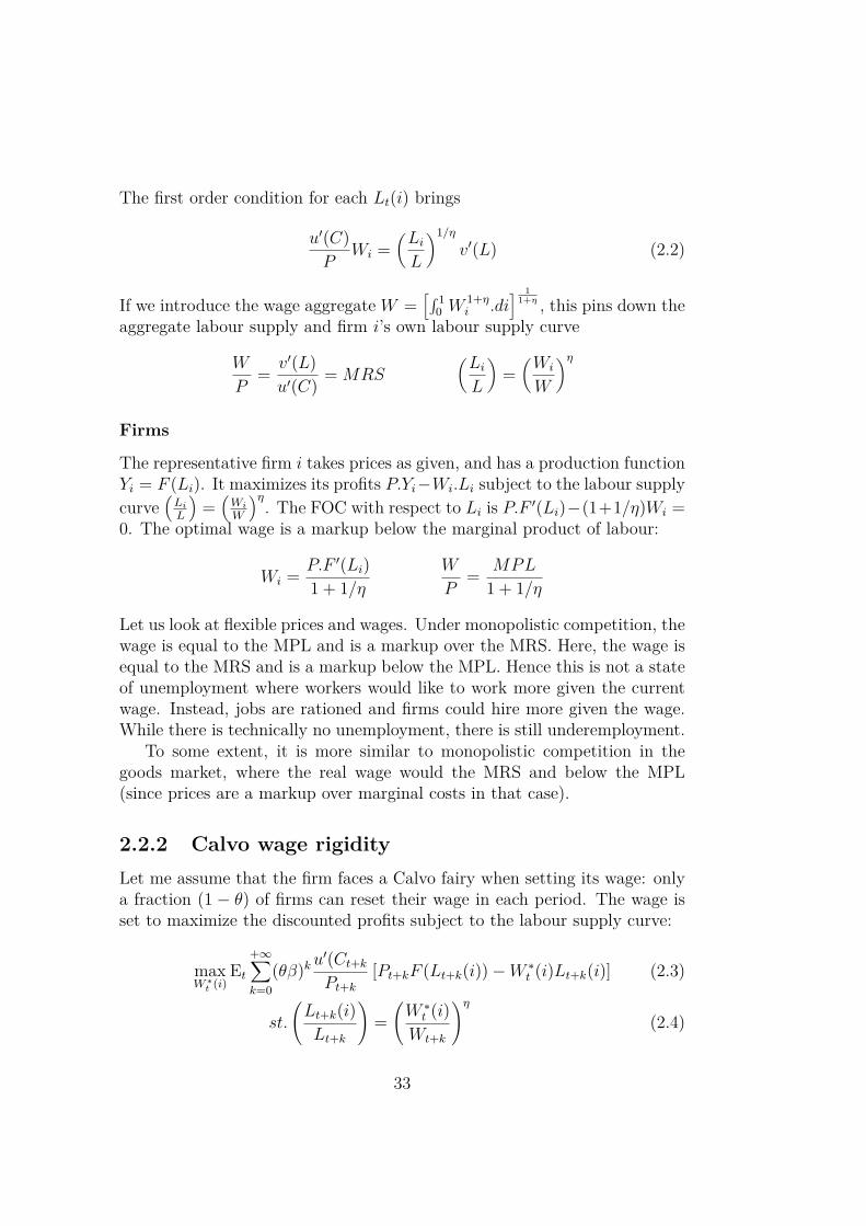
The first order condition for each Lt(i) brings

u′(C)P

Wi =(LiL

)1/ηv′(L) (2.2)

If we introduce the wage aggregate W =[∫ 1

0 W1+ηi .di

] 11+η , this pins down the

aggregate labour supply and firm i’s own labour supply curve

W

P= v′(L)u′(C) = MRS

(LiL

)=(Wi

W

)η

Firms

The representative firm i takes prices as given, and has a production functionYi = F (Li). It maximizes its profits P.Yi−Wi.Li subject to the labour supplycurve

(LiL

)=(Wi

W

)η. The FOC with respect to Li is P.F ′(Li)−(1+1/η)Wi =

0. The optimal wage is a markup below the marginal product of labour:

Wi = P.F ′(Li)1 + 1/η

W

P= MPL

1 + 1/η

Let us look at flexible prices and wages. Under monopolistic competition, thewage is equal to the MPL and is a markup over the MRS. Here, the wage isequal to the MRS and is a markup below the MPL. Hence this is not a stateof unemployment where workers would like to work more given the currentwage. Instead, jobs are rationed and firms could hire more given the wage.While there is technically no unemployment, there is still underemployment.

To some extent, it is more similar to monopolistic competition in thegoods market, where the real wage would the MRS and below the MPL(since prices are a markup over marginal costs in that case).

2.2.2 Calvo wage rigidityLet me assume that the firm faces a Calvo fairy when setting its wage: onlya fraction (1 − θ) of firms can reset their wage in each period. The wage isset to maximize the discounted profits subject to the labour supply curve:

maxW ∗t (i)

Et

+∞∑k=0

(θβ)ku′(Ct+kPt+k

[Pt+kF (Lt+k(i))−W ∗t (i)Lt+k(i)] (2.3)

st.

(Lt+k(i)Lt+k

)=(W ∗t (i)

Wt+k

)η(2.4)

33

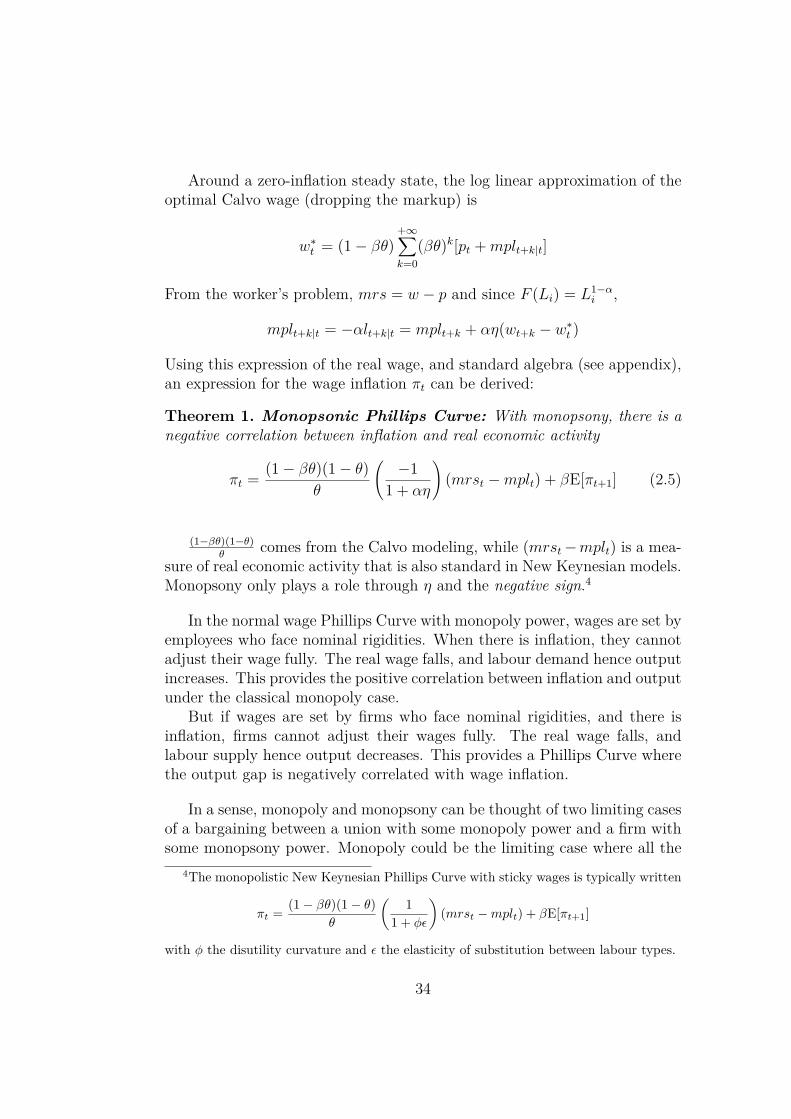
Around a zero-inflation steady state, the log linear approximation of theoptimal Calvo wage (dropping the markup) is

w∗t = (1− βθ)+∞∑k=0

(βθ)k[pt +mplt+k|t]

From the worker’s problem, mrs = w − p and since F (Li) = L1−αi ,

mplt+k|t = −αlt+k|t = mplt+k + αη(wt+k − w∗t )

Using this expression of the real wage, and standard algebra (see appendix),an expression for the wage inflation πt can be derived:

Theorem 1. Monopsonic Phillips Curve: With monopsony, there is anegative correlation between inflation and real economic activity

πt = (1− βθ)(1− θ)θ

(−1

1 + αη

)(mrst −mplt) + βE[πt+1] (2.5)

(1−βθ)(1−θ)θ

comes from the Calvo modeling, while (mrst−mplt) is a mea-sure of real economic activity that is also standard in New Keynesian models.Monopsony only plays a role through η and the negative sign.4

In the normal wage Phillips Curve with monopoly power, wages are set byemployees who face nominal rigidities. When there is inflation, they cannotadjust their wage fully. The real wage falls, and labour demand hence outputincreases. This provides the positive correlation between inflation and outputunder the classical monopoly case.

But if wages are set by firms who face nominal rigidities, and there isinflation, firms cannot adjust their wages fully. The real wage falls, andlabour supply hence output decreases. This provides a Phillips Curve wherethe output gap is negatively correlated with wage inflation.

In a sense, monopoly and monopsony can be thought of two limiting casesof a bargaining between a union with some monopoly power and a firm withsome monopsony power. Monopoly could be the limiting case where all the

4The monopolistic New Keynesian Phillips Curve with sticky wages is typically written

πt = (1− βθ)(1− θ)θ

(1

1 + φε

)(mrst −mplt) + βE[πt+1]

with φ the disutility curvature and ε the elasticity of substitution between labour types.

34

power and surplus accrues to the union/workers, while monopsony would bethe situation where all the power and surplus accrues to the firm. Lookingat the intermediate case can then provide insights about what happens whenthere is a gradual shift of power from one side to the other.

In the next section, I attempt to build such a generalised bargainingmodel that encompasses monopoly and monopsony as the two limiting cases.

2.3 Phillips curve with Nash bargaining

I construct a model with both monopoly power for workers and monopsonypower for firms. I assume that a firm employs a continuum of workers, anda worker works with a continuum of firms. Each pair of worker and firm is amatch. I assume a two-stage process: in the second stage, there is bargainingover the match-specific surplus, while the first-stage bargaining shares thetotal surplus of the worker and the firm. The imperfect substitutability offirms and workers takes place in the second stage but not the first stage.The result of the second stage is to create a labour bargain curve L(w) thatshares the surplus of the match. In the first stage, the bargaining maximizesthe joint aggregate surplus, subject to the labour bargain curve. 5

I assume a modified version of Manning’s (1987) model:6 In the firststage, the firm and worker bargain over the wage, and in the second stagethey bargain over employment. Hence the second stage provides a functionL(w): for each wage there is a bargained level of employment. But Nashbargaining is most often done over a payment or a rate, not a quantity. Itmakes more sense to assume that the agents in the second stage behave asif they were bargaining over the wage, for a given employment.

If there is a project of size L, the firm and worker bargain over the wagecompensationWL over a wage or a payoff makes more sense than bargainingover quantities. This provides a function w(L), a wage for each amount ofwork, which implicitly defines the reciprocal function L(w).

5There is no commitment between the two stages because the agents bargain over adifferent surplus in each stage, and it is as if the agents were different in the two stages.From the first stage point of view, the second stage is done by a representative firm andworker not the the first stage agents. One way to think about it could be that the secondstage features an individual worker and an individual employer, while the first stage wouldbe conducted by a sectoral union and a sectoral business group.

6See section 5 for a critical discussion of this model, and a comparison with the literatureon collective bargaining in general, and in particular the differences with Manning’s model.

35

The surplus of the match

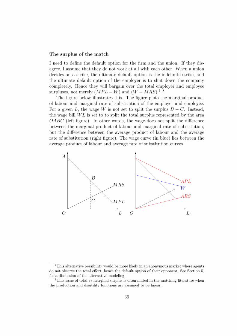
I need to define the default option for the firm and the union. If they dis-agree, I assume that they do not work at all with each other. When a uniondecides on a strike, the ultimate default option is the indefinite strike, andthe ultimate default option of the employer is to shut down the companycompletely. Hence they will bargain over the total employer and employeesurpluses, not merely (MPL−W ) and (W −MRS).7 8

The figure below illustrates this. The figure plots the marginal productof labour and marginal rate of substitution of the employer and employee.For a given L, the wage W is not set to split the surplus B − C. Instead,the wage bill WL is set to to split the total surplus represented by the areaOABC (left figure). In other words, the wage does not split the differencebetween the marginal product of labour and marginal rate of substitution,but the difference between the average product of labour and the averagerate of substitution (right figure). The wage curve (in blue) lies between theaverage product of labour and average rate of substitution curves.

-

6

O

A

B

C

L

MPL

MRS

@@@@@@@@@@@@

-

6

Li

@@@@@@@@@@

O

ARS

HHHHHH

HHHHHHAPL

XXXXXXXXXXXXW

7This alternative possibility would be more likely in an anonymous market where agentsdo not observe the total effort, hence the default option of their opponent. See Section 5,for a discussion of the alternative modeling.

8This issue of total vs marginal surplus is often muted in the matching literature whenthe production and disutility functions are assumed to be linear.

36

2.3.1 Model and flexible equilibriumI introduce the representative production and disutility functions

Assumption 1. (1) Production is a function of a concave labour aggregate

F (L) = L1−α with L1−1/ε =∫ 1

i=0L

1−1/εi di (2.6)

(2) Labour disutility is a function of a convex labour aggregate

v(L) = L1+φ with L1+1/η =∫ 1

j=0L

1+1/ηj dj (2.7)

(3) Concavity of the production function requires 1 > α > 1/ε > 0;Convexity of the disutility requires φ > 1/η > 0 9

payoff functions in the two stage

I can now introduce the payoff functions of the agents in the two stages.

Lemma 7. First StageIn the first stage, the payoffs of the firm and worker depend on the aggre-

gate labour Li and wage Wi that they agree together. Respectively,

pf (Li,Wi) = F (Li)−WiLiP

and pw(Li,Wi) = WiLiP− v(Li)u′(C) (2.8)

A worker working an aggregate L has a marginal disutility of working Liwith firm i: ∂v

∂Li=(LiL

)1/ηv′(L) while a firm employing an aggregate L and Li

from worker i has a marginal product with him writing ∂F∂Li

=(LiL

)−1/εF ′(L)

Hence, conditional on aggregate L, the total surplus of the match is

S(Li|L) =∫ Li

l=0

( lL

)−1/ε

MPL−(l

L

)1/η

MRS

.dlS(Li|L) = ε

ε− 1L

1−1/εi

L−1/ε MPL− η

η + 1L

1+1/ηi

L1/η MRS

Let me now write the second stage payoffs, which depend on match specificemployment Li and wage Wi, as well as aggregate labour L

9This provides the concavity/convexity of the production/disutility with respect toeach Li or Lj , but also with respect to the number of varieties

37

Lemma 8. Second StageIn the second stage, the payoff of the firm (in real terms) is

Pf (Li,Wi|L) = ε

ε− 1L

1−1/εi

L−1/ε MPL− WiLiP

(2.9)

The worker’s payoff in the second stage is, in terms of the goods

Pw(Li,Wi|L) = WiLiP− η

η + 1L

1+1/ηi

L1/η MRS (2.10)

Second stage bargaining

In each match, the wage bargaining is as follows: for each level of employmentLi in the match, the wage bill WiLi maximizes the Nash product

maxWi

Pw(Li,Wi|L)γPf (Li,Wi|L)1−γ

γ and (1− γ) are the bargaining power of the employee and the firm respec-tively. As a result, the wage bill is a weighted average of the total productionand disutility in the match.

Theorem 2. Labour bargain curveThe second stage defines the relationship between Wi and Li in the match,

for a given level of employment L (and hence given MRS and MPL).

Wi

P= (1− γ) η

η + 1

(LiL

)1/ηMRS + γ

ε

ε− 1

(LiL

)−1/εMPL (2.11)

and the labour bargain elasticity is e = ∂ lnLi∂ lnWi

|W,L

This model does not boil down exactly to the usual model of monopoly,or the monopsony one I have introduced previously, when γ = 1 or γ = 0.

When γ = 1, Wi

P= ε

ε−1

(LiL

)−1/εMPL = ε

ε−1MMPL(Li). In a classicalmodel of monopolistic unions, the firm would take the wage and equalize themarginal match product of labour with the wage. However, here, the workeris able to extract more than his MMPL, because he is able to capture thesurplus that he generates for the firm. From a contract theory point of view,this is price discrimination instead of linear pricing.

Similarly, when γ = 0, Wi

P= η

η+1

(LiL

)1/ηMRS = η

η+1MMRS(Li). Thewage is below the worker’s MMRS, because the firm captures the totalsurplus generated by the match.

38

First stage bargaining

Having derived a match specific labour bargain curve, I can now turn to thefirst stage of the bargaining. In the match bargaining, each worker is facingone type of firm, and each firm is facing one type of worker. However, inthe first stage, when the wage and employment is decided, workers are nowfacing the continuum of firms, and firms face the continuum of workers.

The payoff of the worker now is WiLiP− v(Li)

u′(C) and the payoff of the firm isF (Li)− WiLi

P. The Nash bargaining maximizes the joint product, subject to

the labour bargain curve:

maxWi,Li

[γ ln

(WiLiP− v(Li)u′(C)

)+ (1− γ) ln

(F (Li)−

WiLiP

)](2.12)

stWi

P= (1− γ) η

η + 1

(LiL

)1/ηMRS + γ

ε

ε− 1

(LiL

)−1/εMPL

This yields an efficient, symmetric equilibrium when prices are flexible

Theorem 3. Irrespective of γ, the flexible symmetric equilibrium always has

MPL = MRS =(

1 + 1e

)W

P(2.13)

e = ∂ lnLi∂ lnWi

|W,L, the labour bargain elasticity around the steady state, satisfies

1e

=(1−γ)η+1 −

γε−1

(1− γ) ηη+1 + γ ε

ε−1or 1

e+ 1 = (1− γ)η + 1 −

γ

ε− 1

We can look at three particular values for γ

Property 4. (1) When γ = 1, e = −ε and we have perfect monopoly:

MPL = MRS =(

1− 1ε

)W

Pand Wi

W=(LiL

)−1/ε

(2) When γ = 0, e = η and we have perfect monopsony:

MPL = MRS =(

1 + 1η

)W

Pand Wi

W=(LiL

)1/η

(3) When γε−1 = (1−γ)

η+1 , the bargain is isomorphic to perfect competition:WP

= MPL = MRS and labour in a match is perfectly elastic: 1e

= 0

39

It is first worthy to note that the MPL and MRS are equal, but candiffer from the wage. This is due to the assumption of bargaining over thetotal surplus. As a result, since the wage lies between the average product oflabour and average disutility of work, it can be above or below. Of course,this might no longer be efficient with capital or entry in the labour market:the incentives to invest or search for a job would be altered. But here, as weabstract from this, the outcome is always efficient.

Second, this model, which allows the bargaining power to vary betweenthe union and the firm, is able to encompass monopoly and monopsony as thetwo limiting cases. As the bargaining shifts smoothly in the interior of theinterval, the slope of the Phillips curve smoothly changes sign. Also, withthis model, perfect competition and flexible prices can be thought as thecase where the relative bargaining power of employers and employees exactlyoffsets their relative market power coming from the imperfect substitutability.

2.3.2 The wage bargain Phillips curveUnder flexible wages, the timing of the game didn’t really matter. The secondstage featured a bargaining over the wage Wi (or compensation WiLi) in theatomistic match i, for a given match labour Li. Since wages were flexible,they could be agreed on in the second stage as a normal wage bargaining.

However, this isn’t as straightforward in the case of rigid wages. I have toassume that agents in the second stage behave as if they could bargain overthe wage, despite the sticky wage having been decided in the first stage. Sothe second stage bargaining described previously will still apply when wagesare rigid, and the bargained wage is a weighted average of the MPL andMRS. Since it provides a relationship between the wage and the labour inthe match, this relationship can then be used to provide a level of employmentLi for each wage Wi. 10

Payoff functions and Nash problem

With Calvo wage rigidity, the firm and worker maximize a joint product ofpayoffs. The discounted payoff of the worker and the firm are, respectively

Pw =+∞∑k=0

(βθ)k(u′(Ct+k)Pt+k

WtLt+k|t − v(Lt+k|t))

Pf =+∞∑k=0

(βθ)ku′(Ct+k)Pt+k

(Pt+kF (Lt+k|t)−WtLt+k|t

)10See section 5 for a further discussion of this assumption

40

Hence the maximization problem is11

maxWt

P γwP

1−γf st ∂ lnWi

∂ lnLi|W,L = 1

e

First order approximation

I take the first order condition with respect toWt, and around a zero inflationequilibrium, I can use MRS = MPL =

(1 + 1

e

)WP. (see appendix)

The log linear approximation around the steady stare becomes

γ+∞∑k=0

(βθ)k (w∗t − pt+k −mrst+k|t)∑+∞k=0(βθ)k

(1− Pv(L)

u′(C)WL

)=(1− γ)

+∞∑k=0

(βθ)k (w∗t − pt+k −mplt+k|t)∑+∞k=0(βθ)k

(PF (L)WL

− 1) (2.14)

Around the steady state, the denominators in the previous equationsare constant, and can be greatly simplified under the assumption of constantcurvature for the production and disutility function. This constant curvatureis also helpful for an expression of the labour supplied at time t+ k to a firmwhose wage was set at time t (and the labour demanded at t + k from aworker whose wage was set at time t).

Lemma 9. Under the assumption that F (L) = L1−α and v(L) = L1+φ,(1) The steady state labour satisfies

PF (L)WL

− 1 =1e

+ α

1− α and 1− Pv(L)u′(C)WL

=φ− 1

e

1 + φ

(2 )At time (t+ k), the log linear approximation of the MRS and MPL is

mrst+k|t = mrst+k + eφ(w∗t − wt+k)mplt+k|t = mplt+k − eα(w∗t − wt+k)

Taking logs of equation (2.13) in theorem 2, the log of the real wage is

wt+k − pt+k = (1− γ)mrst+k + γmplt+k

with γ = γ εε−1

(1−γ) ηη+1 +γ ε

ε−1= γ ε

ε−1ee+1

All this combined, the log linear approximation provides a Phillips Curve11Gertler and Trigari (2009) also have a model of bargaining with staggered wage ad-

justments, and their bargaining also maximizes a joint product of two discounted payoffs

41

Theorem 4. Nash Bargaining Phillips Curve

πt = (1− βθ)(1− θ)θ

λ (mrst −mplt) + βπt+1 (2.15)

with a slope coefficient

λ =γ2(1+φ)(1+1/e)

φ−1/eεε−1 + (1−γ)2(1−α)(1+1/e)

α+1/eηη+1

γ (1 + φ) + (1− γ) (1− α)

(−1e

)

The coefficient (1−βθ)(1−θ)θ

simply comes from Calvo rigidities, and is com-mon in any Calvo New Keynesian model. (mrst −mplt) = (φlt + σct) + αltthe measure of real economic activity, is also standard in monetary models.Here the relative power of monopoly and monopsony is in the coefficient λ.

Property 5. From property (1), we have φ > 1/η and α > 1/ε, so−α < 1/e < φ. Hence the slope of the Phillips Curve solely depends on

−1e

=γε−1 −

(1−γ)η+1

(1− γ) ηη+1 + γ ε

ε−1

(1) If γε−1 >

(1−γ)η+1 (monopolistic competition), −1

e> 0, the slope is positive

(2) If (1−γ)η+1 > γ

ε−1 (monopsonistic case), −1e> 0, the slope is negative

(3) When γε−1 = (1−γ)

η+1 , the Phillips curve is flat

This model provides a tractable reduced-form Phillips Curve that encom-passes both monopoly and monopsony power, and depends on the relativebargaining power of workers and firms. With both monopoly and monopsonypower, the sign of the slope depends on the relative bargaining power of thetwo sides, as well as the built-in market power that arises from the imperfectsubstitutability of employees for firms and jobs for workers. 12

It is easy to verify that the cases γ = 1 and γ = 0 give the normalmonopoly and monopsony Phillips curves respectively. As with other Calvomodels of the Phillips Curve, this is only an approximation valid around azero inflation steady state where output is equal to its natural level. 13

12If one side does not have market power at all (ε or η is infinite), then a shift ofbargaining power would not change the sign of the slope, but only its magnitude

13But here the natural rate of output around which the log linear approximation is doneis also the first-best efficient outcome

42

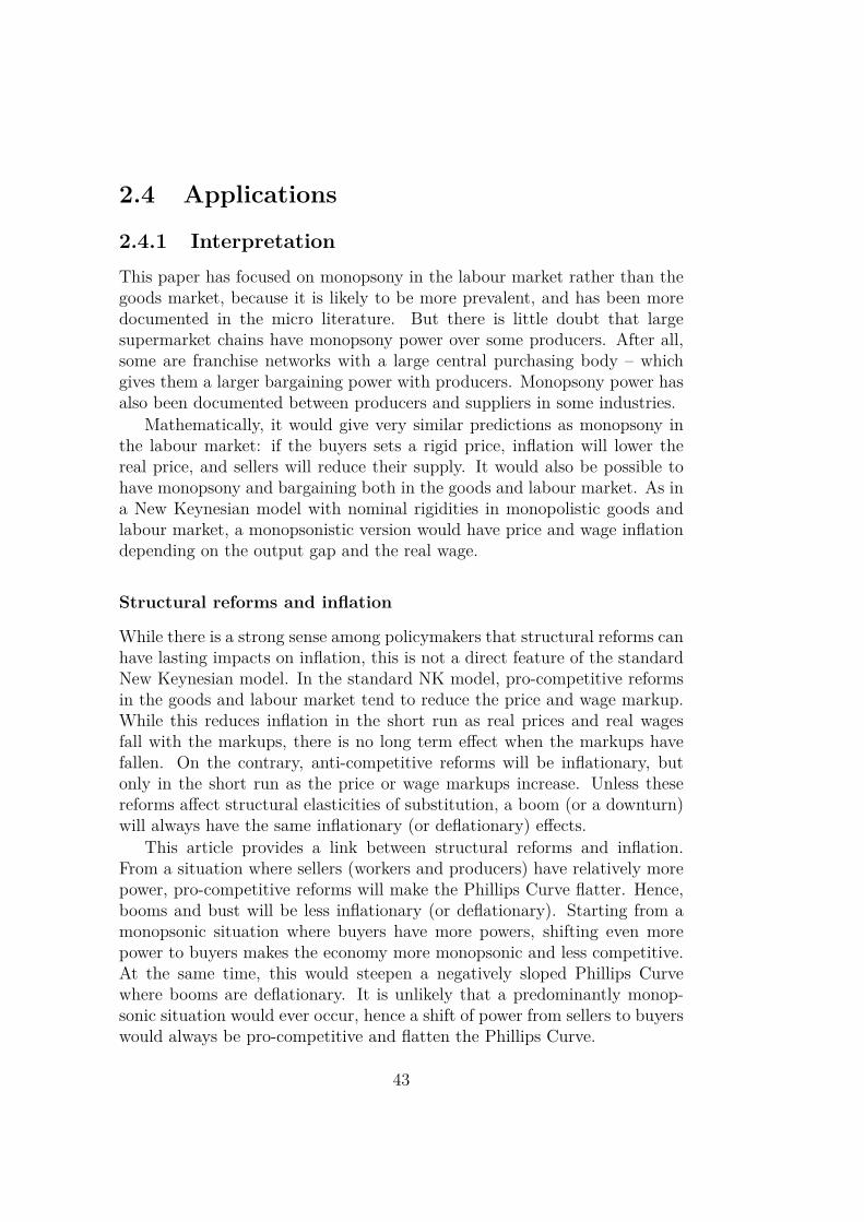
2.4 Applications

2.4.1 InterpretationThis paper has focused on monopsony in the labour market rather than thegoods market, because it is likely to be more prevalent, and has been moredocumented in the micro literature. But there is little doubt that largesupermarket chains have monopsony power over some producers. After all,some are franchise networks with a large central purchasing body – whichgives them a larger bargaining power with producers. Monopsony power hasalso been documented between producers and suppliers in some industries.

Mathematically, it would give very similar predictions as monopsony inthe labour market: if the buyers sets a rigid price, inflation will lower thereal price, and sellers will reduce their supply. It would also be possible tohave monopsony and bargaining both in the goods and labour market. As ina New Keynesian model with nominal rigidities in monopolistic goods andlabour market, a monopsonistic version would have price and wage inflationdepending on the output gap and the real wage.

Structural reforms and inflation

While there is a strong sense among policymakers that structural reforms canhave lasting impacts on inflation, this is not a direct feature of the standardNew Keynesian model. In the standard NK model, pro-competitive reformsin the goods and labour market tend to reduce the price and wage markup.While this reduces inflation in the short run as real prices and real wagesfall with the markups, there is no long term effect when the markups havefallen. On the contrary, anti-competitive reforms will be inflationary, butonly in the short run as the price or wage markups increase. Unless thesereforms affect structural elasticities of substitution, a boom (or a downturn)will always have the same inflationary (or deflationary) effects.

This article provides a link between structural reforms and inflation.From a situation where sellers (workers and producers) have relatively morepower, pro-competitive reforms will make the Phillips Curve flatter. Hence,booms and bust will be less inflationary (or deflationary). Starting from amonopsonic situation where buyers have more powers, shifting even morepower to buyers makes the economy more monopsonic and less competitive.At the same time, this would steepen a negatively sloped Phillips Curvewhere booms are deflationary. It is unlikely that a predominantly monop-sonic situation would ever occur, hence a shift of power from sellers to buyerswould always be pro-competitive and flatten the Phillips Curve.

43

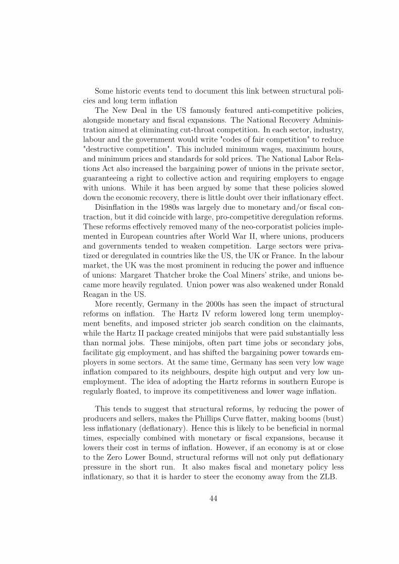
Some historic events tend to document this link between structural poli-cies and long term inflation

The New Deal in the US famously featured anti-competitive policies,alongside monetary and fiscal expansions. The National Recovery Adminis-tration aimed at eliminating cut-throat competition. In each sector, industry,labour and the government would write "codes of fair competition" to reduce"destructive competition". This included minimum wages, maximum hours,and minimum prices and standards for sold prices. The National Labor Rela-tions Act also increased the bargaining power of unions in the private sector,guaranteeing a right to collective action and requiring employers to engagewith unions. While it has been argued by some that these policies sloweddown the economic recovery, there is little doubt over their inflationary effect.

Disinflation in the 1980s was largely due to monetary and/or fiscal con-traction, but it did coincide with large, pro-competitive deregulation reforms.These reforms effectively removed many of the neo-corporatist policies imple-mented in European countries after World War II, where unions, producersand governments tended to weaken competition. Large sectors were priva-tized or deregulated in countries like the US, the UK or France. In the labourmarket, the UK was the most prominent in reducing the power and influenceof unions: Margaret Thatcher broke the Coal Miners’ strike, and unions be-came more heavily regulated. Union power was also weakened under RonaldReagan in the US.

More recently, Germany in the 2000s has seen the impact of structuralreforms on inflation. The Hartz IV reform lowered long term unemploy-ment benefits, and imposed stricter job search condition on the claimants,while the Hartz II package created minijobs that were paid substantially lessthan normal jobs. These minijobs, often part time jobs or secondary jobs,facilitate gig employment, and has shifted the bargaining power towards em-ployers in some sectors. At the same time, Germany has seen very low wageinflation compared to its neighbours, despite high output and very low un-employment. The idea of adopting the Hartz reforms in southern Europe isregularly floated, to improve its competitiveness and lower wage inflation.

This tends to suggest that structural reforms, by reducing the power ofproducers and sellers, makes the Phillips Curve flatter, making booms (bust)less inflationary (deflationary). Hence this is likely to be beneficial in normaltimes, especially combined with monetary or fiscal expansions, because itlowers their cost in terms of inflation. However, if an economy is at or closeto the Zero Lower Bound, structural reforms will not only put deflationarypressure in the short run. It also makes fiscal and monetary policy lessinflationary, so that it is harder to steer the economy away from the ZLB.

44

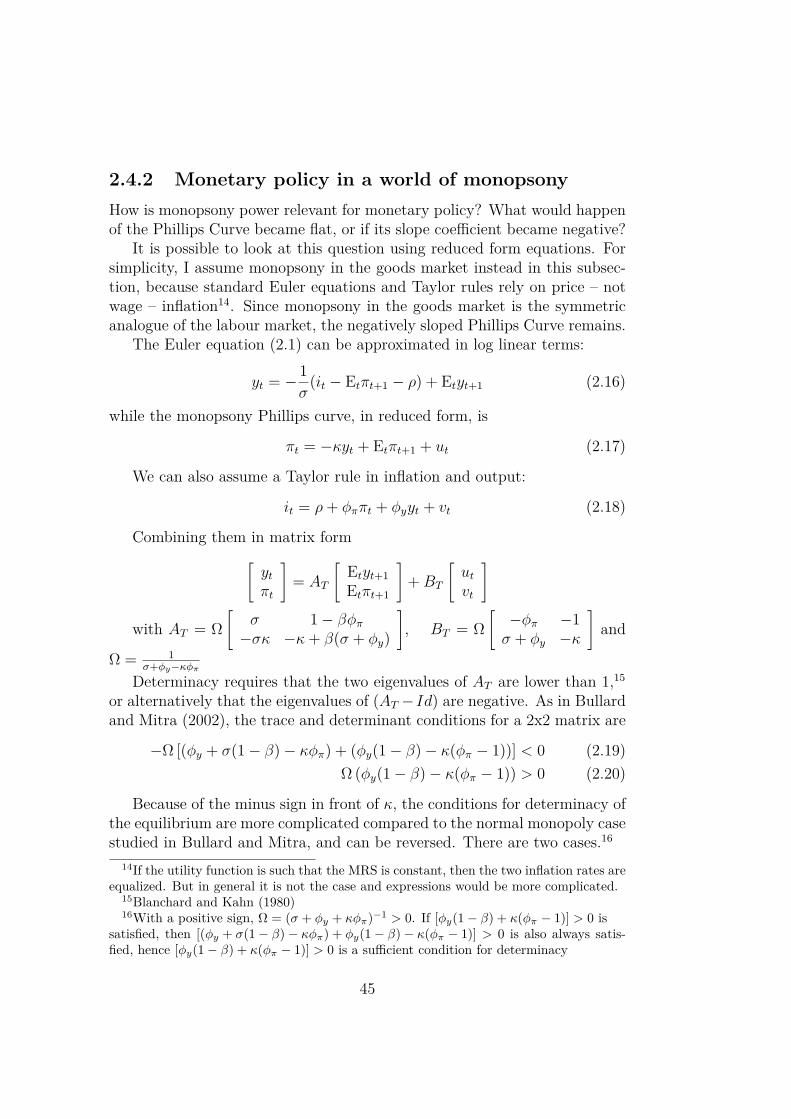
2.4.2 Monetary policy in a world of monopsonyHow is monopsony power relevant for monetary policy? What would happenof the Phillips Curve became flat, or if its slope coefficient became negative?

It is possible to look at this question using reduced form equations. Forsimplicity, I assume monopsony in the goods market instead in this subsec-tion, because standard Euler equations and Taylor rules rely on price – notwage – inflation14. Since monopsony in the goods market is the symmetricanalogue of the labour market, the negatively sloped Phillips Curve remains.

The Euler equation (2.1) can be approximated in log linear terms:

yt = − 1σ

(it − Etπt+1 − ρ) + Etyt+1 (2.16)

while the monopsony Phillips curve, in reduced form, is

πt = −κyt + Etπt+1 + ut (2.17)

We can also assume a Taylor rule in inflation and output:

it = ρ+ φππt + φyyt + vt (2.18)

Combining them in matrix form[ytπt

]= AT

[Etyt+1Etπt+1

]+BT

[utvt

]

with AT = Ω[

σ 1− βφπ−σκ −κ+ β(σ + φy)

], BT = Ω

[−φπ −1σ + φy −κ

]and

Ω = 1σ+φy−κφπ

Determinacy requires that the two eigenvalues of AT are lower than 1,15

or alternatively that the eigenvalues of (AT − Id) are negative. As in Bullardand Mitra (2002), the trace and determinant conditions for a 2x2 matrix are

−Ω [(φy + σ(1− β)− κφπ) + (φy(1− β)− κ(φπ − 1))] < 0 (2.19)Ω (φy(1− β)− κ(φπ − 1)) > 0 (2.20)

Because of the minus sign in front of κ, the conditions for determinacy ofthe equilibrium are more complicated compared to the normal monopoly casestudied in Bullard and Mitra, and can be reversed. There are two cases.16

14If the utility function is such that the MRS is constant, then the two inflation rates areequalized. But in general it is not the case and expressions would be more complicated.

15Blanchard and Kahn (1980)16With a positive sign, Ω = (σ + φy + κφπ)−1 > 0. If [φy(1− β) + κ(φπ − 1)] > 0 is

satisfied, then [(φy + σ(1− β)− κφπ) + φy(1− β)− κ(φπ − 1)] > 0 is also always satis-fied, hence [φy(1− β) + κ(φπ − 1)] > 0 is a sufficient condition for determinacy

45

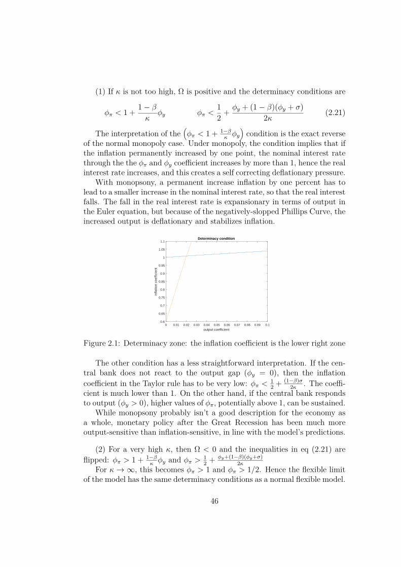
(1) If κ is not too high, Ω is positive and the determinacy conditions are

φπ < 1 + 1− βκ

φy φπ <12 + φy + (1− β)(φy + σ)

2κ (2.21)

The interpretation of the(φπ < 1 + 1−β

κφy)condition is the exact reverse

of the normal monopoly case. Under monopoly, the condition implies that ifthe inflation permanently increased by one point, the nominal interest ratethrough the the φπ and φy coefficient increases by more than 1, hence the realinterest rate increases, and this creates a self correcting deflationary pressure.

With monopsony, a permanent increase inflation by one percent has tolead to a smaller increase in the nominal interest rate, so that the real interestfalls. The fall in the real interest rate is expansionary in terms of output inthe Euler equation, but because of the negatively-slopped Phillips Curve, theincreased output is deflationary and stabilizes inflation.

0 0.01 0.02 0.03 0.04 0.05 0.06 0.07 0.08 0.09 0.1

output coefficient

0.6

0.65

0.7

0.75

0.8

0.85

0.9

0.95

1

1.05

1.1

infla

tion

coef

ficie

nt

Determinacy condition

Figure 2.1: Determinacy zone: the inflation coefficient is the lower right zone

The other condition has a less straightforward interpretation. If the cen-tral bank does not react to the output gap (φy = 0), then the inflationcoefficient in the Taylor rule has to be very low: φπ < 1

2 + (1−β)σ2κ . The coeffi-

cient is much lower than 1. On the other hand, if the central bank respondsto output (φy > 0), higher values of φπ, potentially above 1, can be sustained.

While monopsony probably isn’t a good description for the economy asa whole, monetary policy after the Great Recession has been much moreoutput-sensitive than inflation-sensitive, in line with the model’s predictions.

(2) For a very high κ, then Ω < 0 and the inequalities in eq (2.21) areflipped: φπ > 1 + 1−β

κφy and φπ > 1

2 + φy+(1−β)(φy+σ)2κ

For κ→∞, this becomes φπ > 1 and φπ > 1/2. Hence the flexible limitof the model has the same determinacy conditions as a normal flexible model.

46

2.5 Robustness of the model

2.5.1 Labour aggregatesMicrofoundations for constant elasticities

How can we model monopsony in the labour market? There needs to beimperfect substitutability between different firms or occupations. Of coursemost employees only work with one company – the gig economy where anemployee faces many employers is still a tiny fraction of the workforce.

But even if individuals perfectly substitute, there can still be imperfectaggregate substitutability. Take the Hotelling or Salop model: firms arelocated on a line or a circle, and a mass of consumers is evenly distributed onthe line or circle. Workers can choose where they want to work, but face atransportation cost linked to their distance from the firm. Each worker onlyworks for a single firm, but since workers are distributed over a continuousinterval, some will work for one company and others for another company.A firm will attract more labour by paying a higher wage, but this will notattract the whole mass of workers: there is imperfect substitutability.

Instead of using the Salop or Hotelling model, I will try to remain asclose as possible to the usual monopolistic CES setup, because a CES can bemodeled as the aggregate of probabilistic individuals. Assume N firms. Anindividual j can allocate his time among the N firms. But for each firm i,he has a particular distaste ai,j for the job. The disutility of working is

v

(N∑i=1

ai,jLi,j

)

where Li,j is labour supplied by j to firm i. There is perfect substitutabilityacross jobs. The worker maximizes a separable utility

u

(∑Ni=1wiLi,jP

)− v

(N∑i=1

ai,jLi,j

)

Worker j chooses to work (only) for the company with the highest (wi/ai,j).If the (ai,j) are independent random variables, then the number of workersin firm i is the probability that it has the highest ratio for one individual:

Li = P [wi/ai,j > maxk 6=i

(wk/ak,j)]

Now, if the (ai,j) follow an appropriate Frechet distribution as in Eaton andKortum (2002), this can provide a CES structure: Li

Lk=(Wi

Wk

)ηwith a one to

one mapping between η and the parameters of the Frechet distribution.

47

Labour aggregates with non constant elasticities

Assuming a constant elasticity of substitution for the labour aggregates,the production function and the disutility function makes the model moretractable, but it is not essential. I can assume the more general form for theproduction function and its corresponding labour aggregate:17 Y = F (L)with

L = g−1[∫ 1

i=0g(Li)di

]I can assume a general labour disutility function with its correspondinglabour aggregate:18 v(L) with

L = h−1[∫ 1

j=0h(Lj)dj

]The match product of labour and match rate of substitution are now

TMPL(Li) = g(Li)g′(L)MPL and TMRS(Lj) = h(Lj)

h′(L)MRS

Property 6. Define(η, ε, α, φ, α, φ

)locally by 1

η= Lh′(L)

h(L) −1, 1ε

= 1− Lg′(L)g(L) ,

α = 1− LF ′(L)F (L) , φ = Lv′(L)

v(L) − 1, α = −LF ′′(L)F ′(L) and φ = Lv′′(L)

v′(L)(1) Theorem (3) is unaffected: the steady state expression of the wage

and the labour bargain elasticity with η and ε remain unchanged(2) The Phillips curve in eq (2.15) simply has a modified slope coefficient

λ =γ2(1+φ)φ−1/e

1+1/e1−1/ε + (1−γ)2(1−α)

α+1/e1+1/e1+1/η

γ(1 + φ

)φ−1/eφ−1/e + (1− γ) (1− α) α+1/e

α+1/e

(−1e

)

Since(φ− 1/e

),(φ− 1/e

), (α + 1/e) and (α + 1/e) are all strictly posi-

tive19, the sign of the slope still only depends on(−1e

).

2.5.2 The bargaining assumptionsrelation with the literature and the Manning model

While there is no existing model that combines monopolistic and monopson-istic power together, the labour literature on collective bargaining has some

17Both F (·) and g(·) are increasing, concave function satisfying F (0) = g(0) = 0. Con-cavity of production requires that F (g−1(·)) is also concave, which is a stronger condition

18Both v(·) and h(·) are increasing, convex function satisfying v(0) = h(0) = 0. Con-vexity of disutility requires that v(h−1(·)) is also convex, which is a stronger condition

19Concavity and convexity assumptions on production and disutility require φ > 1/η,φ > 1/η, α > 1/ε and α > 1/ε

48

related elements, in micro models with just one firm and one union. Some-times called a bilateral monopoly it is de-facto a monopoly and a monopsony.

In the right-to-manage model of Nickell and Andrews (1983), the unionand the firm bargain over a wage in the first stage, but in the second stagethe firm is free to choose employment as it sees fit. But this implies that thesecond-stage labour demand curve gives no role to bargaining. McDonaldand Solow (1981) consider a model where the union and the firm bargainsimultaneously over wages and employment, but the simultaneity doesn’tallow for a second stage labour curve. Manning (1987) builds a two stagemodel where the firm and the union first bargain over the wage, and overemployment in the second stage. Given a wage w, the firm would like todemand Ld(w) while the union would like to supply Ls(w). The bargainedemployment L∗(w) will maximize a Nash product of the payoffs.

While Manning’s two-stage timing is very appealing, this model does fea-ture some dubious axiomatic properties that come from the way the second-stage modeled. First, the Nash bargaining is done over employment, for agiven wage, while Nash bargaining is most often done over a price or payment.More importantly, since the bargained labour L∗(w) is some form of averageof the labour demand and the labour supply, the labour bargain curve willend up steeper than the demand or supply curve. Applied to the context ofmonopoly and monopsony power with imperfect substitutability, the result-ing labour bargain curve when bargaining power is more or less balanced willbe steeper, as if substitutability was lower than under either pure monopolyor monopsony. The labour bargain curve could be perfectly inelastic, whichwould be very problematic in the first stage of the bargaining. Last, if eitherthe labour demand or supply is perfectly elastic (with a linear productionfunction or a linear disutility from labour), the labour bargain curve wouldalso be perfectly elastic, irrespective of the bargaining power.

Instead of bargaining over employment, for a given wage, I assumed thatthe firm and union behave as if they were bargaining over the wage, for agiven employment. This has a few advantages. First, this labour bargaincurve will always be more elastic than the pure monopoly or monopsonycurve, and cannot be inelastic. In a sense, when the bargaining power is bal-anced between the firm and union, this is as if there was perfect competition.Hence perfect competition can be thought as a well-balanced market.

Alternative bargaining

I have assumed that there are two stages of Nash bargaining, and the workerand firm have the same relative bargaining power in the two stages. Thisis however not crucial. If the bargaining power were different in the two

49

stages, this would imply minimal changes for the coefficient λ. Crucially,what matters for the elasticity e, and hence the sign of the slope of thePhillips curve, is the bargaining power in the second stage match bargaining.

I have assumed that a firm and a worker share the total surplus of theirmatch, because the default option is to not work with each other at all. Ifinstead, I assume that the default option is to work one hour less with eachother, the labour bargain curve would be

Wi

P= (1− γ)

(LiL

)1/ηMRS + γ

(LiL

)−1/εMPL

One consequence is that the flexible steady state is no longer efficient: in gen-eral: MRS 6= MPL. For low and high values of γ, we have MPL > MRS,which ensures that the surplus of a match is positive. But for intermediatevalues this is not the case, so that the match "surplus" would be negative.In the range where bargaining occurs, it is possible to define an appropri-ate steady state and labour bargain elasticity. The log linear approximationaround the (new) steady state is the same as equation (2.14):

γ∑+∞

k=0(βθ)k[w∗t−pt+k−mrst+k|t]∑+∞k=0(βθ)k

(1− Pv(L)

u′(C)WL

) = (1− γ)∑+∞

k=0(βθ)k[w∗t−pt+k−mplt+k|t]∑+∞k=0(βθ)k(PF (L)

WL−1)

Lemma (1) still holds and provides a log linear MRS and MPL

Now however, since MPL 6= MRS in steady state, the log linear approx-imation of the real wage in equation (2.13) is slightly modified:

wt+k − pt+k = (1− γ)(MRS)mrst+k + γ(MPL)mplt+k(1− γ)MRS + γMPL

A Phillips Curve can still be built, by adjusting the coefficient λ

50

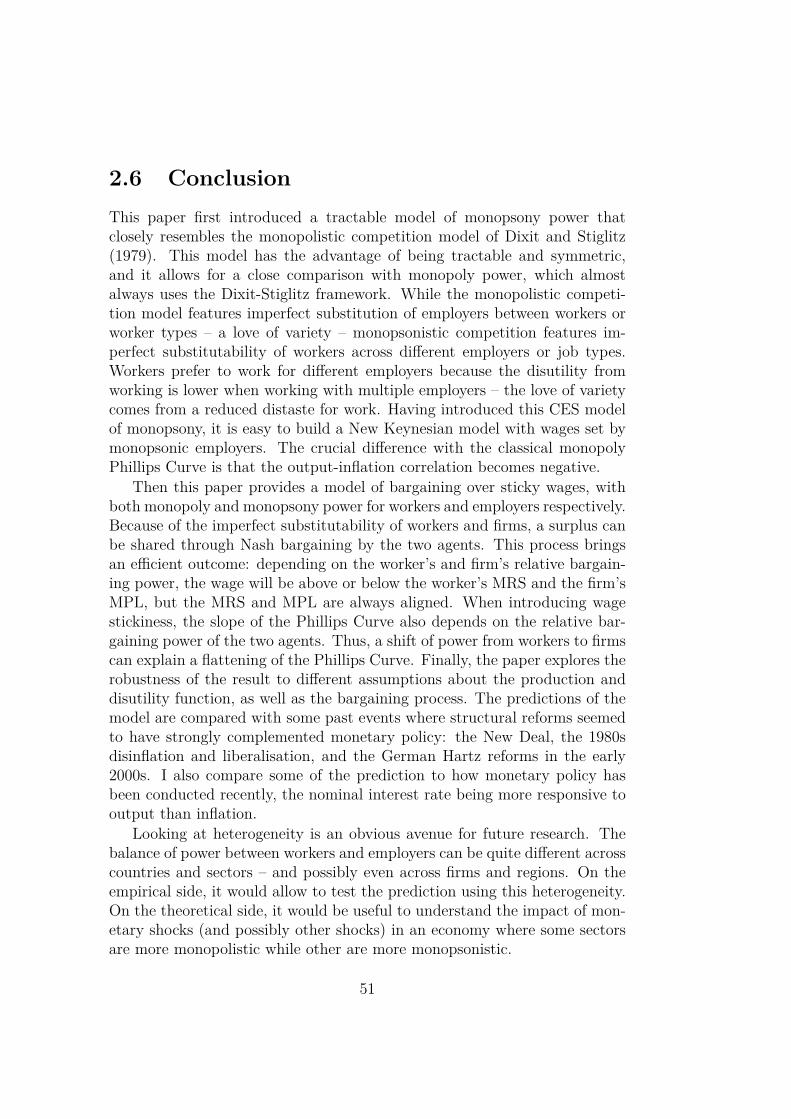
2.6 ConclusionThis paper first introduced a tractable model of monopsony power thatclosely resembles the monopolistic competition model of Dixit and Stiglitz(1979). This model has the advantage of being tractable and symmetric,and it allows for a close comparison with monopoly power, which almostalways uses the Dixit-Stiglitz framework. While the monopolistic competi-tion model features imperfect substitution of employers between workers orworker types – a love of variety – monopsonistic competition features im-perfect substitutability of workers across different employers or job types.Workers prefer to work for different employers because the disutility fromworking is lower when working with multiple employers – the love of varietycomes from a reduced distaste for work. Having introduced this CES modelof monopsony, it is easy to build a New Keynesian model with wages set bymonopsonic employers. The crucial difference with the classical monopolyPhillips Curve is that the output-inflation correlation becomes negative.

Then this paper provides a model of bargaining over sticky wages, withboth monopoly and monopsony power for workers and employers respectively.Because of the imperfect substitutability of workers and firms, a surplus canbe shared through Nash bargaining by the two agents. This process bringsan efficient outcome: depending on the worker’s and firm’s relative bargain-ing power, the wage will be above or below the worker’s MRS and the firm’sMPL, but the MRS and MPL are always aligned. When introducing wagestickiness, the slope of the Phillips Curve also depends on the relative bar-gaining power of the two agents. Thus, a shift of power from workers to firmscan explain a flattening of the Phillips Curve. Finally, the paper explores therobustness of the result to different assumptions about the production anddisutility function, as well as the bargaining process. The predictions of themodel are compared with some past events where structural reforms seemedto have strongly complemented monetary policy: the New Deal, the 1980sdisinflation and liberalisation, and the German Hartz reforms in the early2000s. I also compare some of the prediction to how monetary policy hasbeen conducted recently, the nominal interest rate being more responsive tooutput than inflation.

Looking at heterogeneity is an obvious avenue for future research. Thebalance of power between workers and employers can be quite different acrosscountries and sectors – and possibly even across firms and regions. On theempirical side, it would allow to test the prediction using this heterogeneity.On the theoretical side, it would be useful to understand the impact of mon-etary shocks (and possibly other shocks) in an economy where some sectorsare more monopolistic while other are more monopsonistic.

51

52

Chapter 3

Featherbedding,wage bargaining,and labour market reforms

53

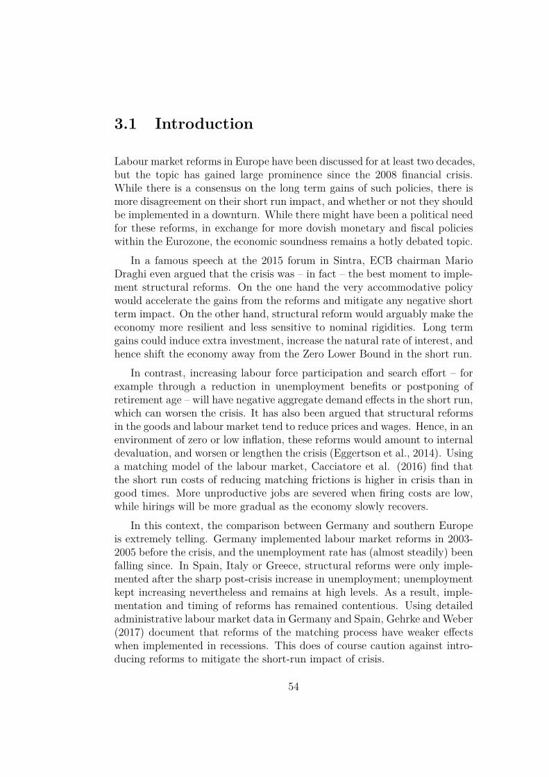
3.1 Introduction

Labour market reforms in Europe have been discussed for at least two decades,but the topic has gained large prominence since the 2008 financial crisis.While there is a consensus on the long term gains of such policies, there ismore disagreement on their short run impact, and whether or not they shouldbe implemented in a downturn. While there might have been a political needfor these reforms, in exchange for more dovish monetary and fiscal policieswithin the Eurozone, the economic soundness remains a hotly debated topic.

In a famous speech at the 2015 forum in Sintra, ECB chairman MarioDraghi even argued that the crisis was – in fact – the best moment to imple-ment structural reforms. On the one hand the very accommodative policywould accelerate the gains from the reforms and mitigate any negative shortterm impact. On the other hand, structural reform would arguably make theeconomy more resilient and less sensitive to nominal rigidities. Long termgains could induce extra investment, increase the natural rate of interest, andhence shift the economy away from the Zero Lower Bound in the short run.

In contrast, increasing labour force participation and search effort – forexample through a reduction in unemployment benefits or postponing ofretirement age – will have negative aggregate demand effects in the short run,which can worsen the crisis. It has also been argued that structural reformsin the goods and labour market tend to reduce prices and wages. Hence, in anenvironment of zero or low inflation, these reforms would amount to internaldevaluation, and worsen or lengthen the crisis (Eggertson et al., 2014). Usinga matching model of the labour market, Cacciatore et al. (2016) find thatthe short run costs of reducing matching frictions is higher in crisis than ingood times. More unproductive jobs are severed when firing costs are low,while hirings will be more gradual as the economy slowly recovers.

In this context, the comparison between Germany and southern Europeis extremely telling. Germany implemented labour market reforms in 2003-2005 before the crisis, and the unemployment rate has (almost steadily) beenfalling since. In Spain, Italy or Greece, structural reforms were only imple-mented after the sharp post-crisis increase in unemployment; unemploymentkept increasing nevertheless and remains at high levels. As a result, imple-mentation and timing of reforms has remained contentious. Using detailedadministrative labour market data in Germany and Spain, Gehrke and Weber(2017) document that reforms of the matching process have weaker effectswhen implemented in recessions. This does of course caution against intro-ducing reforms to mitigate the short-run impact of crisis.

54

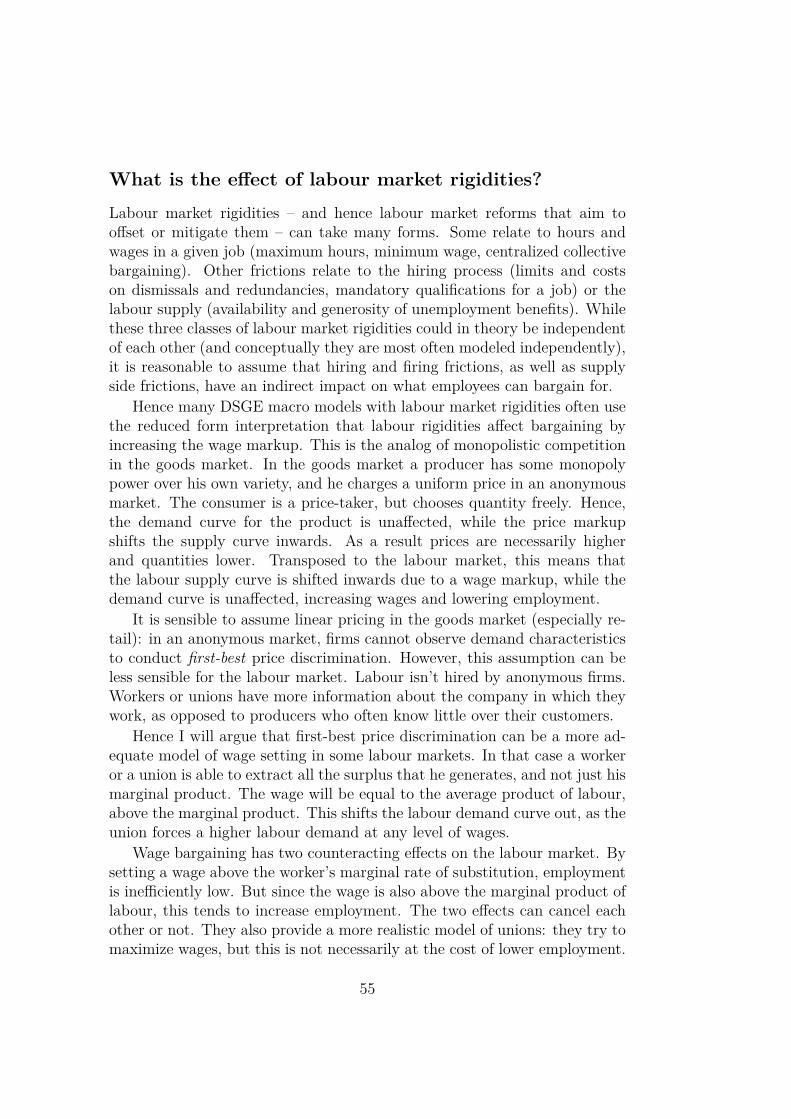
What is the effect of labour market rigidities?Labour market rigidities – and hence labour market reforms that aim tooffset or mitigate them – can take many forms. Some relate to hours andwages in a given job (maximum hours, minimum wage, centralized collectivebargaining). Other frictions relate to the hiring process (limits and costson dismissals and redundancies, mandatory qualifications for a job) or thelabour supply (availability and generosity of unemployment benefits). Whilethese three classes of labour market rigidities could in theory be independentof each other (and conceptually they are most often modeled independently),it is reasonable to assume that hiring and firing frictions, as well as supplyside frictions, have an indirect impact on what employees can bargain for.

Hence many DSGE macro models with labour market rigidities often usethe reduced form interpretation that labour rigidities affect bargaining byincreasing the wage markup. This is the analog of monopolistic competitionin the goods market. In the goods market a producer has some monopolypower over his own variety, and he charges a uniform price in an anonymousmarket. The consumer is a price-taker, but chooses quantity freely. Hence,the demand curve for the product is unaffected, while the price markupshifts the supply curve inwards. As a result prices are necessarily higherand quantities lower. Transposed to the labour market, this means thatthe labour supply curve is shifted inwards due to a wage markup, while thedemand curve is unaffected, increasing wages and lowering employment.

It is sensible to assume linear pricing in the goods market (especially re-tail): in an anonymous market, firms cannot observe demand characteristicsto conduct first-best price discrimination. However, this assumption can beless sensible for the labour market. Labour isn’t hired by anonymous firms.Workers or unions have more information about the company in which theywork, as opposed to producers who often know little over their customers.

Hence I will argue that first-best price discrimination can be a more ad-equate model of wage setting in some labour markets. In that case a workeror a union is able to extract all the surplus that he generates, and not just hismarginal product. The wage will be equal to the average product of labour,above the marginal product. This shifts the labour demand curve out, as theunion forces a higher labour demand at any level of wages.

Wage bargaining has two counteracting effects on the labour market. Bysetting a wage above the worker’s marginal rate of substitution, employmentis inefficiently low. But since the wage is also above the marginal product oflabour, this tends to increase employment. The two effects can cancel eachother or not. They also provide a more realistic model of unions: they try tomaximize wages, but this is not necessarily at the cost of lower employment.

55

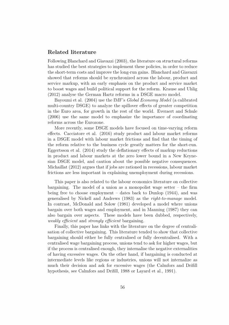
Related literatureFollowing Blanchard and Giavazzi (2003), the literature on structural reformshas studied the best strategies to implement these policies, in order to reducethe short-term costs and improve the long-run gains. Blanchard and Giavazzishowed that reforms should be synchronized across the labour, product andservice markup, with an early emphasis on the product and service marketto boost wages and build political support for the reform. Krause and Uhlig(2012) analyse the German Hartz reforms in a DSGE macro model.

Bayoumi et al. (2004) use the IMF’s Global Economy Model (a calibratedmulti-country DSGE) to analyze the spillover effects of greater competitionin the Euro area, for growth in the rest of the world. Everaert and Schule(2006) use the same model to emphasize the importance of coordinatingreforms across the Eurozone.

More recently, some DSGE models have focused on time-varying reformeffects. Cacciatore et al. (2016) study product and labour market reformsin a DSGE model with labour market frictions and find that the timing ofthe reform relative to the business cycle greatly matters for the short-run.Eggertsson et al. (2014) study the deflationary effects of markup reductionsin product and labour markets at the zero lower bound in a New Keyne-sian DSGE model, and caution about the possible negative consequences.Michaillat (2012) argues that if jobs are rationed in recessions, labour marketfrictions are less important in explaining unemployment during recessions.

This paper is also related to the labour economics literature on collectivebargaining. The model of a union as a monopolist wage setter – the firmbeing free to choose employment – dates back to Dunlop (1944), and wasgeneralised by Nickell and Andrews (1983) as the right-to-manage model.In contrast, McDonald and Solow (1981) developed a model where unionsbargain over both wages and employment, and in Manning (1987) they canalso bargain over aspects. These models have been dubbed, respectively,weakly efficient and strongly efficient bargaining.

Finally, this paper has links with the literature on the degree of centrali-sation of collective bargaining. This literature tended to show that collectivebargaining should either be fully centralised or fully decentralised. With acentralised wage bargaining process, unions tend to ask for higher wages, butif the process is centralised enough, they internalise the negative externalitiesof having excessive wages. On the other hand, if bargaining is conducted atintermediate levels like regions or industries, unions will not internalize asmuch their decision and ask for excessive wages (the Calmfors and Drifillhypothesis, see Calmfors and Drifill, 1988 or Layard et al., 1991).

56

The paper is organised as follows. Section 2 develops a model of differen-tiated workers/unions with monopoly power over employers. If they engagein monopoly pricing, they charge a price and the firm chooses employment.But there is another possibility, that I call featherbedding, where the firmcan be forced to hire more labour than what it wishes given the wage. I showthat given the stock of capital, featherbedding can be efficient, but as it actsas a tax on profits, it vastly reduces 8investment and the level of capital inthe economy. Section 3 looks at structural reforms that reduce the extent offeatherbedding in an economy. The reforms are welfare enhancing becausethey increase the capital stock, but the impact on employment is ambiguous.

3.2 The modelDunlop’s monopoly union model (1944) considered a union setting a wageunilaterally, knowing the labor demand of the firm. This assumption thatthe union can only set a wage, and the firm can choose employment freely,has been generalised by Nickell and Andrews (1983), and is often referredas right-to-manage: hiring and firing is the prerogative of the manager. Incontrast, McDonald and Solow (1981) consider a model where the union andthe firm bargain simultaneously over wages and employment. If the union isable to enforce a level of employment above the firm’s own labour demand,this leads to over-employment, also referred to as featherbedding. This canhowever lead to an efficient contract where over-employment does offset thenegative employment effect of the wage markup.

This paper will compare the right-to-manage and featherbedding models.In the first the union sets a wage, subject to a labour demand curve. Inthe second, the union sets both the wage and the level of employment. Ofcourse, the wage and employment need to be compatible with the firm notmaking a loss, otherwise the plant could simply be shut down entirely. Inthe following subsection I detail the participation constraint of this problem.

3.2.1 Featherbedding: labour demandI model the wage bargaining between a worker and a firm as a principal-agent problem. There are N workers (or worker types), indexed by i. Therepresentative firm has a production function F (L). The aggregate laboursupply L is an aggregate of the labour supplied by each worker i, implicitlydefined by:

g(L) = 1N

N∑i=1

g(Li)

57

Both F (·) and g(·) are increasing, concave function satisfying F (0) = g(0) =0. Concavity of production requires that F (g−1(·)) is also concave, which isa stronger condition.1

If the firm observes a wage Wi and is free to choose the amount of labourLi, the firm’s optimal choice equalizes the marginal surplus with the wage.The marginal surplus product of type-i labour is

MS(Li) = ∂F

∂Li= 1N

g′(Li)g′(L) F

′(L) = 1N

g′(Li)g′(L) MPL (3.1)

On the other hand, if the worker or union of type i is able to choose thewage and employment together, there is a participation constraint: the firmmust be better off acceptingWi and Li than not employing type i at all. Theparticipation constraint is that the total surplus is higher than the wage bill:

TS(Li) = F (L1, . . . , Li, . . . , LN)− F (L1, . . . , Li−1, 0, Li+1, . . . , LN)

= F

[g−1

(1N

N∑k=1

g(Lk))]− F

g−1

1N

∑k 6=i

g(Lk) ≥ WiLi

When N is large, the binding participation constraint can be approximated:

TS(Li) = 1N

g(Li)g′(L)F

′(L) = 1N

g(Li)g′(L)MPL = WiLi

In other words, the wage is the average surplus product of labour

Wi = AS(Li) = TS(Li)Li

= 1N

g(Li)g′(L)Li

MPL (3.2)

Property 7. (1) Under perfect competition and linear pricing, the firm ob-serves the wages (Wi) and chooses its labour demands (Li) to maximize itsprofits. The marginal surplus product of worker i is equal to the wage.

Wi = MS(Li) = 1N

g′(Li)g′(L) MPL

∂ lnWi

∂ lnLi= g′′(Li)Li

g′(Li)

(2) Under price discrimination, the worker of type i is able to capture all ofthe total surplus that he generates for the firm, WiLi = TS(Li), or

Wi = AS(Li) = 1N

g(Li)g′(L)Li

MPL∂ lnWi

∂ lnLi= g′(Li)Li

g(Li)− 1

1For constant elasticities in the production function and labour aggregate, F (L) = L1−α

and L =(

1N

∑Ni=1 L

ε−1ε

i

) εε−1

, these conditions imply 1/ε < α < 1

58

From the concavity of g(·), g(Li)g′(Li)Li > 1 hence AS(Li) > MS(Li)

The labour demand elasticity, ε = − ∂ lnLi∂ lnWi

is equal under (1) and (2) ifg(·) has a constant elasticity of substitution.

Under the featherbedding case, the wage is higher for every level of em-ployment. Or put differently, there is a higher labor demand for every levelof wage. The union imposes a higher demand curve to the firm.

3.2.2 Labour supplyThe household of type i maximize the representative utility function

max E0

+∞∑t=0

βt [u(N.Ct(i))− v(Lt(i))]

subject to a budget constraint

Ct(i) +QtBt(i) = Bt−1(i) +Wt(i)Lt(i) + Dt

N

The numeraire is the homogeneous consumption good Ct.2 The householdreceives a dividend Dt from a diversified equity portfolio, and a wage com-pensation Wt(i)Lt(i). New bonds Bt can be bought or sold at price Qt, thestochastic discount factor of the household. As in Erceg et al. (2000) orGali (2008), let us assume markets with complete contingent claims for con-sumption but not leisure. This ensures full consumption smoothing accrossagents.

Lemma 10. With complete markets, there is full consumption smoothing:

∀(t, i) Ct(i) = CtN

Qt = Etβu′(Ct+1)u′(Ct)

(3.3)

The labour supply decision for a worker i is equivalent to maximizing thefollowing quantity in each period

u′(Ct)Wt(i)Lt(i)− v(Lt(i)) (3.4)

subject to the labour demand curve defined in property (1)2The factor N is simply introduced for scaling reasons as in the labour aggregate previ-

ously. With N symmetric agents, each consumes 1/N of the available total consumption,Ct(i) = Ct/N but the MRS will feature the marginal utility of aggregate consumption

59

Property 8. (1) Under perfect competition, the wage is equal to the marginalrate of substitution, Wi = MRSi

N= 1

Nv′(Li)u′(C)

(2) Under both linear pricing and price discrimination, the wage is amarkup over the MRS, with the elasticity ε = − ∂ lnLi

∂ lnWidefined in property (1)

Wi = 1N

ε

ε− 1MRSi = 1N

ε

ε− 1v′(Li)u′(C)

As a result, both the competitive market and featherbedding case havean efficient level of employment, since the MPL is equal to the MRS. Withlinear pricing, employment is inefficiently low.

I now assume a continuum of workers/unions, to get rid of the factor N :

Theorem 5. In the symmetric equilibrium(1) Under perfect competition W = MPL = MRS

(2) Under linear pricing W = MPL = εε−1MRS with ε = − g′(L)

g′′(L)L(3) Under featherbedding MPL = MRS = ε−1

εW with ε = 1

1− g′(L)Lg(L)

Featherbedding is efficient even though the wage is above the MPL andMRS. However, dividends are abnormally low in this economy:

D = Y −WL = F (L)− ε

ε− 1MPL.L < F (L)−MPL.L

discussion

Labour market rigidities are usually modeled as an employment tax, as itcreates a wedge between the demand and supply of labour. But here, theserigidities are acting instead as a capital income tax. Instead of having awedge between the marginal product of labour and the marginal rate ofsubstitution, featherbedding creates a wedge between the marginal productof capital and the returns to capital, and can be thought of as a tax.

Under featherbedding, unions are not detrimental to employment but toprofits. Conditional on the MPL and MRS curves, featherbedding providesan efficient level of employment and output. But this efficiency is conditionalon a fixed amount of capital. This is no longer the case when I introduceinvestment. Featherbedding makes firms’ profits abnormally low, and thisreduces the steady state level of capital in the economy. Firms under invest,because they will be "held up" once capital is installed (Grout, 1984). Thewedge between the MPK and returns to capital acts as a capital income tax.

60

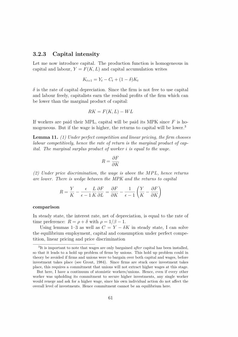
3.2.3 Capital intensityLet me now introduce capital. The production function is homogeneous incapital and labour, Y = F (K,L) and capital accumulation writes

Kt+1 = Yt − Ct + (1− δ)Kt

δ is the rate of capital depreciation. Since the firm is not free to use capitaland labour freely, capitalists earn the residual profits of the firm which canbe lower than the marginal product of capital:

RK = F (K,L)−WL

If workers are paid their MPL, capital will be paid its MPK since F is ho-mogeneous. But if the wage is higher, the returns to capital will be lower.3

Lemma 11. (1) Under perfect competition and linear pricing, the firm chooseslabour competitively, hence the rate of return is the marginal product of cap-ital. The marginal surplus product of worker i is equal to the wage.

R = ∂F

∂K

(2) Under price discrimination, the wage is above the MPL, hence returnsare lower. There is wedge between the MPK and the returns to capital

R = Y

K− ε

ε− 1L

K

∂F

∂L= ∂F

∂K− 1ε− 1

(Y

K− ∂F

∂K

)

comparison

In steady state, the interest rate, net of depreciation, is equal to the rate oftime preference: R = ρ+ δ with ρ = 1/β − 1.

Using lemmas 1–3 as well as C = Y − δK in steady state, I can solvethe equilibrium employment, capital and consumption under perfect compe-tition, linear pricing and price discrimination

3It is important to note that wages are only bargained after capital has been installed,so that it leads to a hold up problem of firms by unions. This hold up problem could intheory be avoided if firms and unions were to bargain over both capital and wages, beforeinvestment takes place (see Grout, 1984). Since firms are stuck once investment takesplace, this requires a commitment that unions will not extract higher wages at this stage.But here, I have a continuum of atomistic workers/unions. Hence, even if every other

worker was upholding its commitment to secure higher investments, any single workerwould renege and ask for a higher wage, since his own individual action do not affect theoverall level of investments. Hence commitment cannot be an equilibrium here.

61

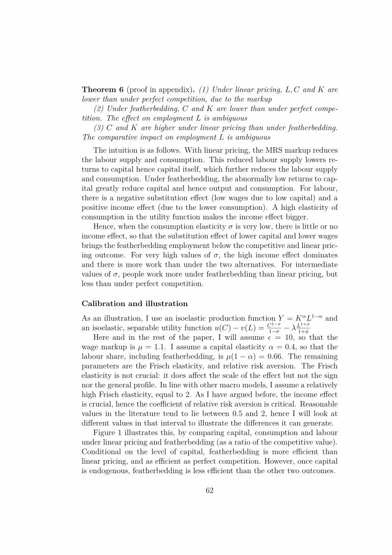
Theorem 6 (proof in appendix). (1) Under linear pricing, L,C and K arelower than under perfect competition, due to the markup

(2) Under featherbedding, C and K are lower than under perfect compe-tition. The effect on employment L is ambiguous

(3) C and K are higher under linear pricing than under featherbedding.The comparative impact on employment L is ambiguous

The intuition is as follows. With linear pricing, the MRS markup reducesthe labour supply and consumption. This reduced labour supply lowers re-turns to capital hence capital itself, which further reduces the labour supplyand consumption. Under featherbedding, the abnormally low returns to cap-ital greatly reduce capital and hence output and consumption. For labour,there is a negative substitution effect (low wages due to low capital) and apositive income effect (due to the lower consumption). A high elasticity ofconsumption in the utility function makes the income effect bigger.

Hence, when the consumption elasticity σ is very low, there is little or noincome effect, so that the substitution effect of lower capital and lower wagesbrings the featherbedding employment below the competitive and linear pric-ing outcome. For very high values of σ, the high income effect dominatesand there is more work than under the two alternatives. For intermediatevalues of σ, people work more under featherbedding than linear pricing, butless than under perfect competition.

Calibration and illustration

As an illustration, I use an isoelastic production function Y = KαL1−α andan isoelastic, separable utility function u(C)− v(L) = C1−σ

1−σ − λL1+φ

1+φHere and in the rest of the paper, I will assume ε = 10, so that the

wage markup is µ = 1.1. I assume a capital elasticity α = 0.4, so that thelabour share, including featherbedding, is µ(1 − α) = 0.66. The remainingparameters are the Frisch elasticity, and relative risk aversion. The Frischelasticity is not crucial: it does affect the scale of the effect but not the signnor the general profile. In line with other macro models, I assume a relativelyhigh Frisch elasticity, equal to 2. As I have argued before, the income effectis crucial, hence the coefficient of relative risk aversion is critical. Reasonablevalues in the literature tend to lie between 0.5 and 2, hence I will look atdifferent values in that interval to illustrate the differences it can generate.

Figure 1 illustrates this, by comparing capital, consumption and labourunder linear pricing and featherbedding (as a ratio of the competitive value).Conditional on the level of capital, featherbedding is more efficient thanlinear pricing, and as efficient as perfect competition. However, once capitalis endogenous, featherbedding is less efficient than the other two outcomes.

62

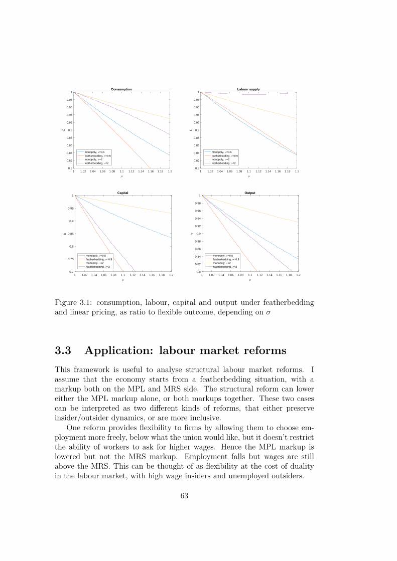
1 1.02 1.04 1.06 1.08 1.1 1.12 1.14 1.16 1.18 1.2

µ

0.8

0.82

0.84

0.86

0.88

0.9

0.92

0.94

0.96

0.98

1

C

Consumption

monopoly, σ=0.5featherbedding, σ=0.5monopoly, σ=2featherbedding, σ=2

1 1.02 1.04 1.06 1.08 1.1 1.12 1.14 1.16 1.18 1.2

µ

0.8

0.82

0.84

0.86

0.88

0.9

0.92

0.94

0.96

0.98

1

L

Labour supply

monopoly, σ=0.5featherbedding, σ=0.5monopoly, σ=2featherbedding, σ=2

1 1.02 1.04 1.06 1.08 1.1 1.12 1.14 1.16 1.18 1.2

µ

0.7

0.75

0.8

0.85

0.9

0.95

1

K

Capital

monopoly, σ=0.5featherbedding, σ=0.5monopoly, σ=2featherbedding, σ=2

1 1.02 1.04 1.06 1.08 1.1 1.12 1.14 1.16 1.18 1.2

µ

0.8

0.82

0.84

0.86

0.88

0.9

0.92

0.94

0.96

0.98

1

YOutput

monopoly, σ=0.5featherbedding, σ=0.5monopoly, σ=2featherbedding, σ=2

Figure 3.1: consumption, labour, capital and output under featherbeddingand linear pricing, as ratio to flexible outcome, depending on σ

3.3 Application: labour market reformsThis framework is useful to analyse structural labour market reforms. Iassume that the economy starts from a featherbedding situation, with amarkup both on the MPL and MRS side. The structural reform can lowereither the MPL markup alone, or both markups together. These two casescan be interpreted as two different kinds of reforms, that either preserveinsider/outsider dynamics, or are more inclusive.

One reform provides flexibility to firms by allowing them to choose em-ployment more freely, below what the union would like, but it doesn’t restrictthe ability of workers to ask for higher wages. Hence the MPL markup islowered but not the MRS markup. Employment falls but wages are stillabove the MRS. This can be thought of as flexibility at the cost of dualityin the labour market, with high wage insiders and unemployed outsiders.

63

The other reform affects both the hiring decision of the firm and the wagedemand of workers. While firms have more freedom to choose a lower levelof employment (the fall in MPL markup), the wage demands of workers alsofall (with the MRS markup). Hence this is a more inclusive reform whichdoesn’t protect wages at the cost of employment.

Allowing the MPL or both markups to fall has immediate consequences onemployment, but it also leads to higher investment driven by higher expectedprofits. Hence in the long run capital increases, which improves the efficiencyof the economy. This improved efficiency has two effects on employment: thehigher capital increases the real wage while increased consumption will lowerthe labour supply. For a very high relative risk aversion, the income effectcan be stronger then the substitution effect.

1 1.02 1.04 1.06 1.08 1.1 1.12 1.14 1.16 1.18 1.2

µ

-0.5

-0.4

-0.3

-0.2

-0.1

0

0.1

0.2

d ln

L /

d µ

σ=0.5σ=1σ=2

(a) MPL markup only

1 1.02 1.04 1.06 1.08 1.1 1.12 1.14 1.16 1.18 1.2

µ

-0.2

0

0.2

0.4

0.6

0.8

1d

ln L

/ d µ

σ=0.5σ=1σ=2

(b) Both markups

Figure 3.2: Marginal (long term) percentage increase in labour with a reduc-tion in one or two of the markups, depending on the relative risk aversionσ

Figure 2 shows the long run percentage change in employment causedby a marginal reduction in one or two of the markups. Not surprisingly,an inclusive reform is better at reducing unemployment. In fact, reducingonly the MPL markup will often lead to a fall in employment in the longrun. This fall in employment is not welfare deteriorating, especially sinceconsumption does increase in the long run hence households consume moreand work less. But this does illustrate that not all structural reforms arebeneficial to employment in the long run.

But in a dynamic model, investment demand will have an additionaleffect on employment. The rest of the section studies when and how thesestructural reforms are beneficial or not to employment in the short run.

64

3.3.1 The dynamic equilibriumI assume an isoelastic production function

Yt = Kαt L

1−αt (3.5)

The utility function is also isoelastic:

+∞∑t=0

βt[u(Ct)− v(Lt)] =+∞∑t=0

βt[C1−σt

1− σ − λL1+φt

1 + φ

]

I assume that the economy starts in a steady state with labour market rigidi-ties, corresponding to what I have described above: the wage is above theMRS and the MPL (the two markups being potentially different4)

Wt = µ1tMRSt = µ1

tLφtC

σt (3.6)

Wt = µ2tMPLt = (1− α)µ2

t

(Kt

Lt

)α(3.7)

The returns to capital is not the MPK, but the residual profits: Rt = Yt−WtLtKt

If capital can be invested freely, the budget constraint and Euler equationare, respectively

Kt+1 = (1− δ)Kt + Yt − Ct (3.8)

C−σt = βEt

[(1− δ + Yt+1 −Wt+1Lt+1

Kt+1

)C−σt+1

](3.9)

I also look at quadratic costs of adjusting capital. The budget constraintand Euler equation now become

Kt+1 = (1− δ)Kt + Yt − Ct − ψ(Kt+1 −Kt)2

2Kt

(3.10)

C−σt = βEt

(1− δ + Yt+1−Wt+1Lt+1Kt+1

− ψKt+1−KtKt

)C−σt+1

+βψKt+2−Kt+1Kt+1

C−σt+2

(3.11)

Equations 3.6, 3.7, and 3.5, combined with 3.8 and 3.9 (or eqs 3.10 and3.11) are a system of 5 equations in Y, K, L C and W. Starting from steadystate values for µ1 and µ2, it is possible to observe the response to a structuralreform shock that would lower either or both of these markups.

4Perfect competition corresponds to the two markups being equal to 1, and linearpricing has the MPL markup equal to 1

65

fall of MPL markup

I will consider first a sudden fall in the MPL markup at time t. This is anunanticipated "MIT shock". The economy was at steady state before, andwill converge to the new steady state without facing any additional shock.But the MRS markup is unaffected: µ2

t−1 = µ1t−1 = µ and

∀T ≥ t, µ2T = µ− ut and µ2

T = µ

I consider the case of flexible investment, as well as medium (ψ = 3) and high(ψ = 10) quadratic costs of adjusting capital. In a downturn, investment isarguably hindered and these high adjustment costs reflect this.

gradual fall of both markups

Later I look at a structural reform that lowers both the MPL and MRSmarkups. However, I assume that these two markups do not fall at the samespeed because realistically, some changes can only be gradual. In particular,even if a policy aims at reducing the two wage markups, it is likely thatthe MPL markup will fall more rapidly than the MRS markup. From asituation of featherbedding, if right-to-manage is introduced (for example byliberalizing layoffs and reducing the scope of tools available to union), theeffects are likely to be rapid. On the other hand, resisting a fall in the MRSmarkup would likely be easier, so that this markup would fall more slowly.

This is not a model of sticky wages. There is a downward rigidity on oneof the wage markups, not on the wage itself. I simply assume that it takestime for workers to accept that their wage markup is falling. Apart from themarkup, the wage does adjust to market changes like capital or investment.

Hence, I modify the previous set of equations as follows. There is a longterm, permanent markup shock ut and the MPL markup falls immediately

∀T ≥ t, µ2T = µ− ut

However, the MRS markup does fall more gradually: µ1t−1 = µ and

∀T ≥ t, µ1T = θµ1

T−1 + (1− θ)(µ− ut)

θ ∈ (0, 1) is a parameter for the persistence of the MRS markup. I assumea relatively high θ = 0.95, that corresponds to strong resistance to a fall inthe wage markup, that is likely to occur if there is downward wage rigidity,particularly in a downturn with low inflation. As with the MPL-only case, Iconsider flexible investment and quadratic costs with ψ = 3 and ψ = 10.

66

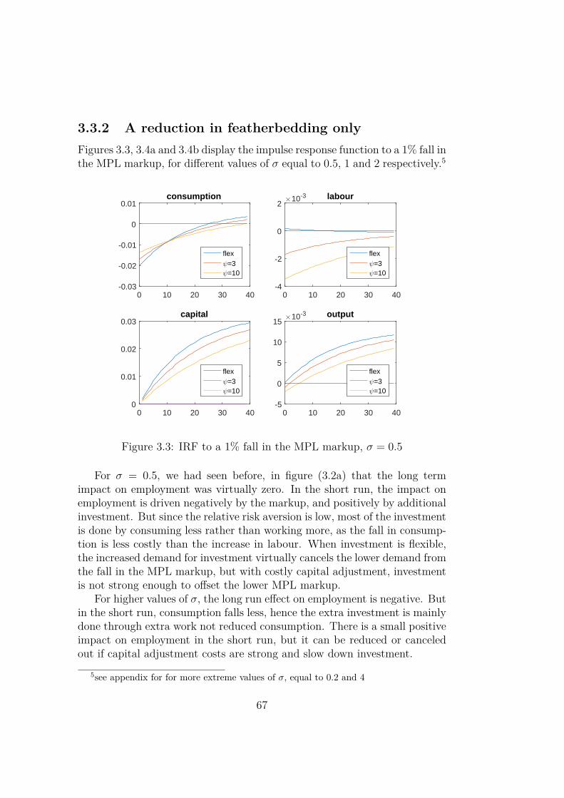
3.3.2 A reduction in featherbedding onlyFigures 3.3, 3.4a and 3.4b display the impulse response function to a 1% fall inthe MPL markup, for different values of σ equal to 0.5, 1 and 2 respectively.5

0 10 20 30 40-0.03

-0.02

-0.01

0

0.01consumption

flexψ=3ψ=10

0 10 20 30 40-4

-2

0

2×10-3 labour

flexψ=3ψ=10

0 10 20 30 400

0.01

0.02

0.03capital

flexψ=3ψ=10

0 10 20 30 40-5

0

5

10

15×10-3 output

flexψ=3ψ=10

Figure 3.3: IRF to a 1% fall in the MPL markup, σ = 0.5

For σ = 0.5, we had seen before, in figure (3.2a) that the long termimpact on employment was virtually zero. In the short run, the impact onemployment is driven negatively by the markup, and positively by additionalinvestment. But since the relative risk aversion is low, most of the investmentis done by consuming less rather than working more, as the fall in consump-tion is less costly than the increase in labour. When investment is flexible,the increased demand for investment virtually cancels the lower demand fromthe fall in the MPL markup, but with costly capital adjustment, investmentis not strong enough to offset the lower MPL markup.

For higher values of σ, the long run effect on employment is negative. Butin the short run, consumption falls less, hence the extra investment is mainlydone through extra work not reduced consumption. There is a small positiveimpact on employment in the short run, but it can be reduced or canceledout if capital adjustment costs are strong and slow down investment.

5see appendix for for more extreme values of σ, equal to 0.2 and 4

67

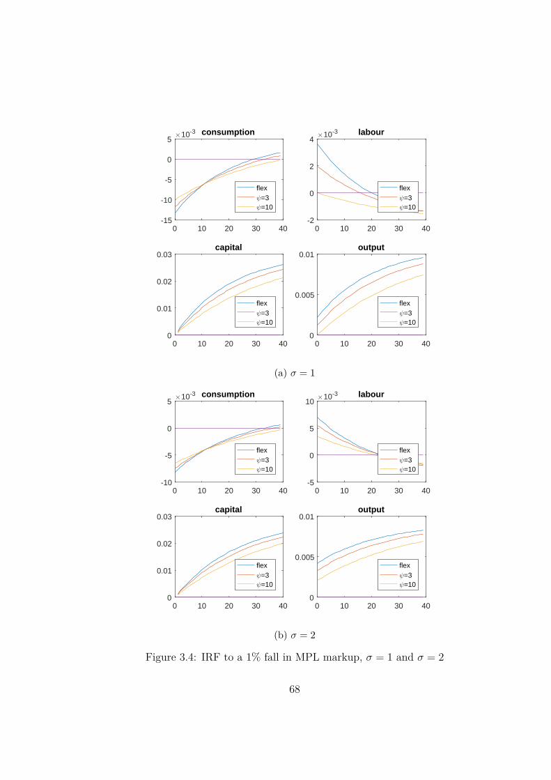
0 10 20 30 40-15

-10

-5

0

5×10-3 consumption

flexψ=3ψ=10

0 10 20 30 40-2

0

2

4×10-3 labour

flexψ=3ψ=10

0 10 20 30 400

0.01

0.02

0.03capital

flexψ=3ψ=10

0 10 20 30 400

0.005

0.01output

flexψ=3ψ=10

(a) σ = 1

0 10 20 30 40-10

-5

0

5×10-3 consumption

flexψ=3ψ=10

0 10 20 30 40-5

0

5

10×10-3 labour

flexψ=3ψ=10

0 10 20 30 400

0.01

0.02

0.03capital

flexψ=3ψ=10

0 10 20 30 400

0.005

0.01output

flexψ=3ψ=10

(b) σ = 2

Figure 3.4: IRF to a 1% fall in MPL markup, σ = 1 and σ = 2

68

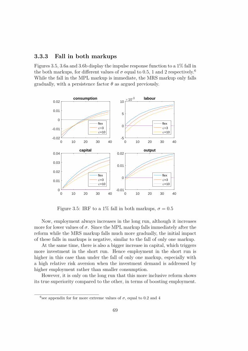
3.3.3 Fall in both markupsFigures 3.5, 3.6a and 3.6b display the impulse response function to a 1% fall inthe both markups, for different values of σ equal to 0.5, 1 and 2 respectively.6While the fall in the MPL markup is immediate, the MRS markup only fallsgradually, with a persistence factor θ as argued previously.

0 10 20 30 40-0.02

-0.01

0

0.01

0.02consumption

flexψ=3ψ=10

0 10 20 30 40-5

0

5

10×10-3 labour

flexψ=3ψ=10

0 10 20 30 400

0.01

0.02

0.03

0.04capital

flexψ=3ψ=10

0 10 20 30 40-0.01

0

0.01

0.02output

flexψ=3ψ=10

Figure 3.5: IRF to a 1% fall in both markups, σ = 0.5

Now, employment always increases in the long run, although it increasesmore for lower values of σ. Since the MPL markup falls immediately after thereform while the MRS markup falls much more gradually, the initial impactof these falls in markups is negative, similar to the fall of only one markup.

At the same time, there is also a bigger increase in capital, which triggersmore investment in the short run. Hence employment in the short run ishigher in this case than under the fall of only one markup, especially witha high relative risk aversion when the investment demand is addressed byhigher employment rather than smaller consumption.

However, it is only on the long run that this more inclusive reform showsits true superiority compared to the other, in terms of boosting employment.

6see appendix for for more extreme values of σ, equal to 0.2 and 4

69

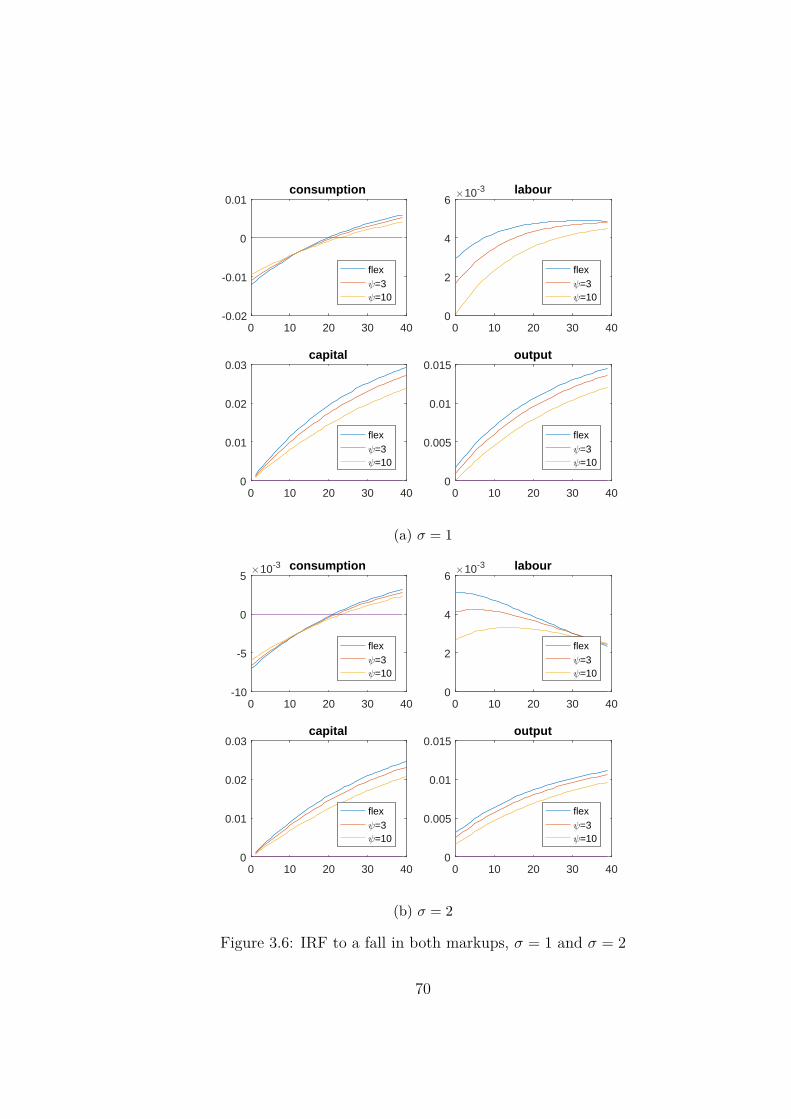
0 10 20 30 40-0.02

-0.01

0

0.01consumption

flexψ=3ψ=10

0 10 20 30 400

2

4

6×10-3 labour

flexψ=3ψ=10

0 10 20 30 400

0.01

0.02

0.03capital

flexψ=3ψ=10

0 10 20 30 400

0.005

0.01

0.015output

flexψ=3ψ=10

(a) σ = 1

0 10 20 30 40-10

-5

0

5×10-3 consumption

flexψ=3ψ=10

0 10 20 30 400

2

4

6×10-3 labour

flexψ=3ψ=10

0 10 20 30 400

0.01

0.02

0.03capital

flexψ=3ψ=10

0 10 20 30 400

0.005

0.01

0.015output

flexψ=3ψ=10

(b) σ = 2

Figure 3.6: IRF to a fall in both markups, σ = 1 and σ = 2

70

3.4 ConclusionIn this paper I have built a model of featherbedding in the labour market,and I have argued that it can be a good description of some sectors or in-dustries where labour unions are relatively strong. I have shown that withfeatherbedding, the wage is a markup over workers’ marginal rate of substi-tution (MRS), but the wage is also a markup over firms’ marginal productof labour. If these two markups are equal, the MPL and MRS are equalised,in contrast to monopoly pricing where there is a markup on the MRS butnot the MPL. However, since the wage is above the MPL, firms’ profits areabnormally low. Hence when capital is introduced, this leads to an ineffi-ciently low level of capital, with ambiguous effect on employment dependingon agents’ relative risk aversion. I argue that with featherbedding labourmarket rigidities act as a tax on capital and not as a tax on labour.

I than considered the impact – particularly on employment – of structuralreforms that aim to reduce the featherbedding rigidity. If the reform onlyallows firm to choose employment more freely without reducing the monopolymarkup of unions, welfare improves, but the short and long term effects onemployment are small or negative. This has resemblance to the insider-outsider literature where reforms that only affect new entrants in the labourmarket tend to be less effective. On the other hand, if the reform lowersboth markups at the same time, welfare improves more, and employmentdoes increase more, or at least fall less. In the short and middle run, theeffect of these two kind of reforms strongly depends on the relative speed ofadjustment of the two markups, and on the easiness with which investmentdemand for labour can offset any negative short term effect.

Using this framework in larger DSGE models is an obvious possibility offuture research. This paper did not introduce nominal rigidities per se, andhas no role for a central bank. But a larger model would enable me to see howa central bank can accompany the structural reform and ease any negativeeffect in the short run. Introducing entry by firms would also make capitaladjustment more gradual, so that short term pain might be lengthened.

While featherbedding is likely more prevalent in the labour market, somesimilar can exist in the market for goods and services. In sectors with verylittle competition, it is not uncommon that consumers have little choice aboutthe amount of goods or services that they can buy, and are forced to buymore than what they would wish. One of the first effects of liberalisation,in such cases, is that new entrants break the one-size-fit-all equilibrium andcater more closely to the needs of the consumer, by selling in more divisiblequantities, or by creating low cost products. The framework of this papercould hence also be used in the goods and labour market.

71

72

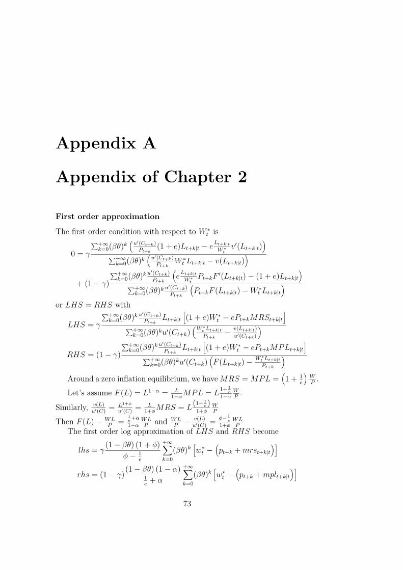
Appendix A

Appendix of Chapter 2

First order approximation

The first order condition with respect to W ∗t is

0 = γ

∑+∞k=0(βθ)k

(u′(Ct+k)Pt+k

(1 + e)Lt+k|t − eLt+k|tW ∗t

v′(Lt+k|t))

∑+∞k=0(βθ)k

(u′(Ct+k)Pt+k

W ∗t Lt+k|t − v(Lt+k|t)

)+ (1− γ)

∑+∞k=0(βθ)k u

′(Ct+k)Pt+k

(eLt+k|tW ∗t

Pt+kF′(Lt+k|t)− (1 + e)Lt+k|t

)∑+∞k=0(βθ)k u′(Ct+k)

Pt+k

(Pt+kF (Lt+k|t)−W ∗

t Lt+k|t)

or LHS = RHS with

LHS = γ

∑+∞k=0(βθ)k u

′(Ct+k)Pt+k

Lt+k|t[(1 + e)W ∗

t − ePt+kMRSt+k|t]

∑+∞k=0(βθ)ku′(Ct+k)

(W ∗t Lt+k|tPt+k

− v(Lt+k|t)u′(Ct+k)

)RHS = (1− γ)

∑+∞k=0(βθ)k u

′(Ct+k)Pt+k

Lt+k|t[(1 + e)W ∗

t − ePt+kMPLt+k|t]

∑+∞k=0(βθ)ku′(Ct+k)

(F (Lt+k|t)−

W ∗t Lt+k|tPt+k

)Around a zero inflation equilibrium, we haveMRS = MPL =

(1 + 1

e

)WP.

Let’s assume F (L) = L1−α = L1−αMPL = L

1+ 1e

1−αWP.

Similarly, v(L)u′(C) = L1+φ

u′(C) = L1+φMRS = L

(1+ 1e)

1+φWP

Then F (L)− WLP

=1e

+α1−α

WLP

and WLP− v(L)

u′(C) = φ− 1e

1+φWLP

The first order log approximation of LHS and RHS become

lhs = γ(1− βθ) (1 + φ)

φ− 1e

+∞∑k=0

(βθ)k[w∗t −

(pt+k +mrst+k|t

)]

rhs = (1− γ)(1− βθ) (1− α)1e

+ α

+∞∑k=0

(βθ)k[w∗t −

(pt+k +mplt+k|t

)]

73

mrst+k|t = mrst+k + φ(lt+k|t − lt+k) = mrst+k + eφ(w∗t − wt+k), so

lhs = γ(1− βθ) (1 + φ)

φ− 1e

+∞∑k=0

(βθ)k [(1− eφ) (w∗t − wt+k) + (wt+k − pt+k)−mrst+k]

mplt+k|t = mrst+k − α(lt+k|t − lt+k) = mplt+k − eα(w∗t − wt+k), so

rhs = (1−γ)(1− βθ) (1− α)1e

+ α

+∞∑k=0

(βθ)k [(1 + eα) (w∗t − wt+k) + (wt+k − pt+k)−mplt+k]

The aggregate wage satisfies WP

= (1− γ) ηη+1MRS + γ ε

ε−1MPL, sowt+k − pt+k = (1− γ)mrst+k + γmplt+k

with γ = γ εε−1

(1−γ) ηη+1 +γ ε

ε−1= γ ε

ε−1ee+1

lhs = γ(1− βθ) (1 + φ)

φ− 1e

+∞∑k=0

(βθ)k[

(1− eφ) (w∗t − wt+k)+γ (mplt+k −mrst+k)

]

rhs = (1− γ)(1− βθ) (1− α)1e

+ α

+∞∑k=0

(βθ)k[

(1 + eα) (w∗t − wt+k)+(1− γ) (mrst+k −mplt+k)

]

Setting lhs = rhs implies

(γ (1 + φ) + (1− γ) (1− α))w∗t

= (1− βθ)+∞∑k=0

(βθ)k[

(γ (1 + φ) + (1− γ) (1− α))wt+k+(γ(1+φ)eφ−1 γ + (1−γ)(1−α)

1+αe (1− γ))

(mplt+k −mrst+k)

]

This can be written recursively as

(w∗t − wt) = (1−βθ)γ(1+φ)eφ−1 γ + (1−γ)(1−α)

1+αe (1− γ)γ (1 + φ) + (1− γ) (1− α) (mrst −mplt)+βθ

(w∗t+1 − wt

)As a result, I get a Phillips curve

πt = (1− βθ)(1− θ)θ

λ (mrst −mplt) + βπt+1

with a slope coefficient

λ =γ(1+φ)φ−1/e γ + (1−γ)(1−α)

α+1/e (1− γ)γ (1 + φ) + (1− γ) (1− α)

(−1e

)

λ =γ2(1+φ)(1+1/e)

φ−1/eεε−1 + (1−γ)2(1−α)(1+1/e)

α+1/eηη+1

γ (1 + φ) + (1− γ) (1− α)

(−1e

)

74

Appendix B

Appendix of Chapter 3

ProofsTheorem 7. (1) Under linear pricing, L,C and K are lower than underperfect competition, due to the markup

(2) Under featherbedding, C and K are lower than under perfect compe-tition. L is ambiguous

(3) C and K are higher under monopoly than under featherbedding. L isambiguous

Proof : (1) write (K,L,C) as a function of the markup µ

MPL(K,L)− µMRS(C,L) = 0MPK(K,L)− (ρ+ δ) = 0

F (K,L)− δK − C = 0

Differentiating this system with a Jacobian,KFKLFL

LFLLFL− Lv′′(L)

v′(L)u′′(C)u′(C)C

KFKK LFKL 0KFK −Kδ LFL −C

∂ lnK∂ lnµ∂ lnL∂ lnµ∂ lnC∂ lnµ

=100

SinceMPL andMPK are homogenous of degree 0 in (K,L), it can be shownthat

∂ lnK∂ lnµ = ∂ lnL

∂ lnµ = ∂ lnC∂ lnµ = −1

σ + φ

with σ and φ the (possibly local) elasticities of the utility of consumptionand disutility of work.

75

(2) write (K,L,C) as a function of the markup µ

MPL(K,L)−MRS(C,L) = 0F (K,L)− µLMPL(K,L)− (ρ+ δ)K = 0

F (K,L)− δK − C = 0

A similar differentiation bringsKFKLFL

LFLLFL− Lv′′(L)

v′(L)u′′(C)u′(C)C

(µ− 1)− µKFKLFL

(1− µ)− µLFLLFL

0KFK −Kδ LFL −C

∂ lnK∂ lnµ∂ lnL∂ lnµ∂ lnC∂ lnµ

=0µ0

Using the (possibly local) elasticities of the production and utility function,this gives

∂ lnK∂ lnµ =

α + φ+ σLFLC

α− (µ−1)µ

−1φ+ σ

<−1φ+ σ

∂ lnC∂ lnµ =

[α + φ (KFK−Kδ)

C

]α− (µ−1)

µ

−1φ+ σ

<−1φ+ σ

∂ lnL∂ lnµ =

α− σ (µ−1)δ(1−α)+ραµδ(1−α)+ρ

α− (µ−1)µ

−1φ+ σ

≷ 0

(3) Comparing the cases (1) and (2) above, one simply needs to look at

∂ lnK∂ lnµ |(2) <

∂ lnK∂ lnµ |(1)

∂ lnC∂ lnµ |(2) <

∂ lnC∂ lnµ |(1)

∂ lnL∂ lnµ |(2) ≷

∂ lnL∂ lnµ |(1)

76

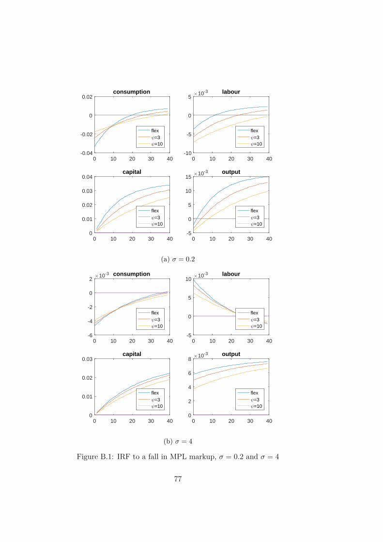
0 10 20 30 40-0.04

-0.02

0

0.02consumption

flexψ=3ψ=10

0 10 20 30 40-10

-5

0

5×10-3 labour

flexψ=3ψ=10

0 10 20 30 400

0.01

0.02

0.03

0.04capital

flexψ=3ψ=10

0 10 20 30 40-5

0

5

10

15×10-3 output

flexψ=3ψ=10

(a) σ = 0.2

0 10 20 30 40-6

-4

-2

0

2×10-3 consumption

flexψ=3ψ=10

0 10 20 30 40-5

0

5

10×10-3 labour

flexψ=3ψ=10

0 10 20 30 400

0.01

0.02

0.03capital

flexψ=3ψ=10

0 10 20 30 400

2

4

6

8×10-3 output

flexψ=3ψ=10

(b) σ = 4

Figure B.1: IRF to a fall in MPL markup, σ = 0.2 and σ = 4

77

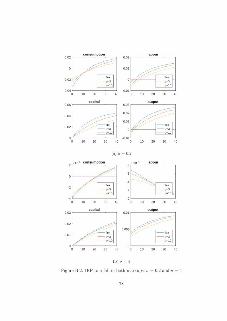
0 10 20 30 40-0.04

-0.02

0

0.02consumption

flexψ=3ψ=10

0 10 20 30 40-0.01

0

0.01

0.02labour

flexψ=3ψ=10

0 10 20 30 400

0.02

0.04

0.06capital

flexψ=3ψ=10

0 10 20 30 40-0.01

0

0.01

0.02

0.03output

flexψ=3ψ=10

(a) σ = 0.2

0 10 20 30 40-4

-2

0

2×10-3 consumption

flexψ=3ψ=10

0 10 20 30 400

2

4

6

8×10-3 labour

flexψ=3ψ=10

0 10 20 30 400

0.01

0.02

0.03capital

flexψ=3ψ=10

0 10 20 30 400

0.005

0.01output

flexψ=3ψ=10

(b) σ = 4

Figure B.2: IRF to a fall in both markups, σ = 0.2 and σ = 4

78

Bibliography

[Akerlof et al., 1996] Akerlof, G. A., Dickens, W. R., and Perry, G. L. (1996).The macroeconomics of low inflation. Brookings Papers on Economic Ac-tivity, 27(1):1–76.

[Ball and Mazumder, 2011] Ball, L. and Mazumder, S. (2011). Inflation Dy-namics and the Great Recession. Brookings Papers on Economic Activity,42(1 (Spring):337–405.

[Bayoumi et al., 2004] Bayoumi, T., Laxton, D., and Pesenti, P. (2004). Ben-efits and spillovers of greater competition in europe: a macroeconomicassessment. Working Paper Series 341, European Central Bank.

[Benigno and Woodford, 2004] Benigno, P. and Woodford, M. (2004). Opti-mal stabilization policy when wages and prices are sticky: The case of adistorted steady state. NBER w10839.

[Benigno and Woodford, 2005] Benigno, P. and Woodford, M. (2005). Infla-tion stabilization and welfare: The case of a distorted steady state. Journalof the European Economic Association, 3(6):1185–1236.

[Bergman and Brannlund, 1995] Bergman, M. A. and Brannlund, R. (1995).Measuring oligopsony power: An application to the swedish pulp and paperindustry. Review of Industrial Organization, 10(3):307–321.

[Bilbiie et al., 2014] Bilbiie, F., Ghironi, F., and Fujiwara, I. (2014). Optimalmonetary policy with endogenous product variety. Journal of MonetaryEconomics, 64:1–20.

[Bilbiie et al., 2012] Bilbiie, F., Ghironi, F., and Melitz, M. (2012). En-dogenous entry, product variety and business cycles. Journal of PoliticalEconomy, 120(2):304–345.

[Bilbiie et al., 2013] Bilbiie, F., Ghironi, F., and Melitz, M. (2013). Mono-poly power and endogenous product variety: Distortions and remedies.NBER WP w14383.

79

[Blanchard, 2016] Blanchard, O. (2016). The us phillips curve: Back to the60s? Peterson Institute for International Economics.

[Blanchard and Gali, 2007] Blanchard, O. and Gali, J. (2007). Real wagerigidities and the new keynesian model. Journal of Money, Credit andBanking, 39:35–65.

[Blanchard and Giavazzi, 2003] Blanchard, O. and Giavazzi, F. (2003).Macroeconomic effects of regulation and deregulation in goods and labormarkets*. The Quarterly Journal of Economics, 118(3):879–907.

[Brendon and Ellison, 2015] Brendon, C. and Ellison, M. (2015). Time-consistent institutional design. mimeo.

[Brown and Medoff, 1989] Brown, C. and Medoff, J. (1989). The employersize-wage effect. Journal of Political Economy, 97(5):1027–1059.

[Cacciatore et al., 2016] Cacciatore, M., Duval, R., Fiori, G., and Ghironi,F. (2016). Market reforms in the time of imbalance. Journal of EconomicDynamics and Control, 72:69 – 93.

[Cahuc and Zylberberg, 2004] Cahuc, P. and Zylberberg, A. (2004). LaborEconomics. The MIT Press.

[Calmfors and Driffill, 1988] Calmfors, L. and Driffill, J. (1988). Bargainingstructure, corporatism and macroeconomic performance. Economic Policy,3(6):14–61.

[Calvo, 1983] Calvo, G. A. (1983). Staggered prices in a utility-maximizingframework. Journal of Monetary Economics, 12(3):383–398.

[Carney, 2017] Carney, M. (2017). [de]globalisation and inflation. 2017 IMFMichel Camdessus Central Banking Lecture.

[Dunlop, 1944] Dunlop, J. (1944). Wage determination under trade unions.New York, NY: Macmillan. New York, NY: Macmillan.

[Eggertsson et al., 2014] Eggertsson, G., Ferrero, A., and Raffo, A. (2014).Can structural reforms help europe? Journal of Monetary Economics,61(C):2–22.

[Erceg et al., 2000] Erceg, C., Henderson, D., and Levin, A. (2000). Opti-mal monetary policy with staggered wage and price contracts. Journal ofMonetary Economics, 46(2):281 – 313.

80

[Everaert and Schule, 2008] Everaert, L. and Schule, W. (2008). Why it paysto synchronize structural reforms in the euro area across markets and coun-tries. IMF Staff Papers, 55(2):356–366.

[Friedman, 1968] Friedman, M. (1968). The role of monetary policy. TheAmerican Economic Review, 58(1):1–17.

[Gabaix, 2016] Gabaix, X. (2016). A behavioral new keynesian model. NBERw22954.

[Gali, 2008] Gali, J. (2008). Monetary Policy, Inflation, and the BusinessCycle: An Introduction to the New Keynesian Framework and Its Applica-tions. Princeton University Press.

[Gali, 2011] Gali, J. (2011). The return of the wage phillips curve. Journalof the European Economic Association, 9(3):436–461.

[Gali and Gertler, 1999] Gali, J. and Gertler, M. (1999). Inflation dynam-ics: A structural econometric analysis. Journal of Monetary Economics,44(2):195 – 222.

[Galuscak et al., 2012] Galuscak, K., Keeney, M., Nicolitsas, D., Smets, F.,Strzelecki, P., and Vodopivec, M. (2012). The determination of wages ofnewly hired employees: Survey evidence on internal versus external factors.Labour Economics, 19(5):802 – 812.

[Gehrke and Weber, 2017] Gehrke, B. and Weber, E. (2017). Identifyingasymmetric effects of labor market reforms. IAB Discussion Paper 201723.

[Gertler et al., 2016] Gertler, M., Huckfeldt, C., and Trigari, A. (2016). Un-employment fluctuations, match quality, and the wage cyclicality of newhires. NBER w22341.

[Gertler and Trigari, 2009] Gertler, M. and Trigari, A. (2009). Unemploy-ment fluctuations with staggered nash wage bargaining. Journal of Polit-ical Economy, 117(1):38–86.

[Green et al., 1996] Green, F., Machin, S., and Manning, A. (1996). The em-ployer size-wage effect: Can dynamic monopsony provide an explanation?Oxford Economic Papers, 48(3):433–455.

[Haldane, 2017] Haldane, A. (2017). Work, wages and monetary policy.speech given at Bradford.

81

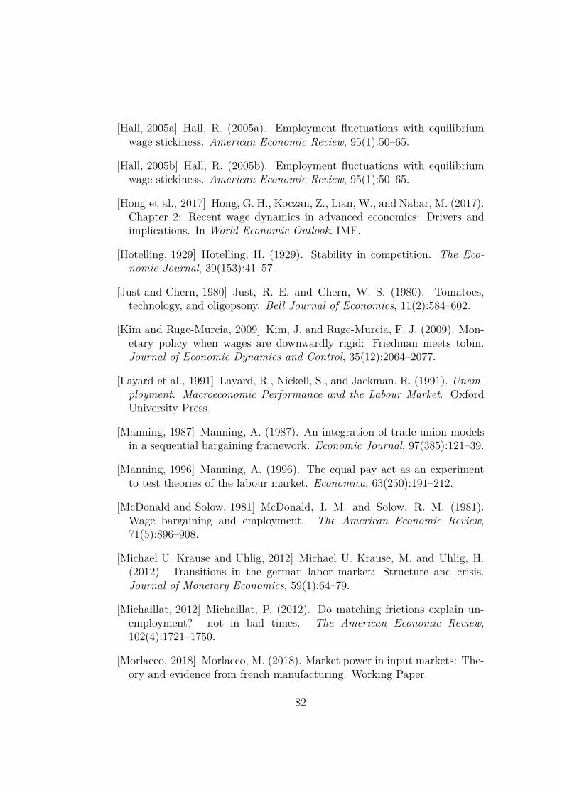
[Hall, 2005a] Hall, R. (2005a). Employment fluctuations with equilibriumwage stickiness. American Economic Review, 95(1):50–65.

[Hall, 2005b] Hall, R. (2005b). Employment fluctuations with equilibriumwage stickiness. American Economic Review, 95(1):50–65.

[Hong et al., 2017] Hong, G. H., Koczan, Z., Lian, W., and Nabar, M. (2017).Chapter 2: Recent wage dynamics in advanced economics: Drivers andimplications. In World Economic Outlook. IMF.

[Hotelling, 1929] Hotelling, H. (1929). Stability in competition. The Eco-nomic Journal, 39(153):41–57.

[Just and Chern, 1980] Just, R. E. and Chern, W. S. (1980). Tomatoes,technology, and oligopsony. Bell Journal of Economics, 11(2):584–602.

[Kim and Ruge-Murcia, 2009] Kim, J. and Ruge-Murcia, F. J. (2009). Mon-etary policy when wages are downwardly rigid: Friedman meets tobin.Journal of Economic Dynamics and Control, 35(12):2064–2077.

[Layard et al., 1991] Layard, R., Nickell, S., and Jackman, R. (1991). Unem-ployment: Macroeconomic Performance and the Labour Market. OxfordUniversity Press.

[Manning, 1987] Manning, A. (1987). An integration of trade union modelsin a sequential bargaining framework. Economic Journal, 97(385):121–39.

[Manning, 1996] Manning, A. (1996). The equal pay act as an experimentto test theories of the labour market. Economica, 63(250):191–212.

[McDonald and Solow, 1981] McDonald, I. M. and Solow, R. M. (1981).Wage bargaining and employment. The American Economic Review,71(5):896–908.

[Michael U. Krause and Uhlig, 2012] Michael U. Krause, M. and Uhlig, H.(2012). Transitions in the german labor market: Structure and crisis.Journal of Monetary Economics, 59(1):64–79.

[Michaillat, 2012] Michaillat, P. (2012). Do matching frictions explain un-employment? not in bad times. The American Economic Review,102(4):1721–1750.

[Morlacco, 2018] Morlacco, M. (2018). Market power in input markets: The-ory and evidence from french manufacturing. Working Paper.

82

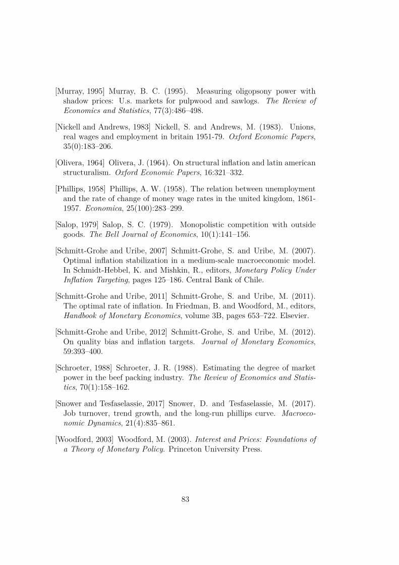
[Murray, 1995] Murray, B. C. (1995). Measuring oligopsony power withshadow prices: U.s. markets for pulpwood and sawlogs. The Review ofEconomics and Statistics, 77(3):486–498.

[Nickell and Andrews, 1983] Nickell, S. and Andrews, M. (1983). Unions,real wages and employment in britain 1951-79. Oxford Economic Papers,35(0):183–206.

[Olivera, 1964] Olivera, J. (1964). On structural inflation and latin americanstructuralism. Oxford Economic Papers, 16:321–332.

[Phillips, 1958] Phillips, A. W. (1958). The relation between unemploymentand the rate of change of money wage rates in the united kingdom, 1861-1957. Economica, 25(100):283–299.

[Salop, 1979] Salop, S. C. (1979). Monopolistic competition with outsidegoods. The Bell Journal of Economics, 10(1):141–156.

[Schmitt-Grohe and Uribe, 2007] Schmitt-Grohe, S. and Uribe, M. (2007).Optimal inflation stabilization in a medium-scale macroeconomic model.In Schmidt-Hebbel, K. and Mishkin, R., editors, Monetary Policy UnderInflation Targeting, pages 125–186. Central Bank of Chile.

[Schmitt-Grohe and Uribe, 2011] Schmitt-Grohe, S. and Uribe, M. (2011).The optimal rate of inflation. In Friedman, B. and Woodford, M., editors,Handbook of Monetary Economics, volume 3B, pages 653–722. Elsevier.

[Schmitt-Grohe and Uribe, 2012] Schmitt-Grohe, S. and Uribe, M. (2012).On quality bias and inflation targets. Journal of Monetary Economics,59:393–400.

[Schroeter, 1988] Schroeter, J. R. (1988). Estimating the degree of marketpower in the beef packing industry. The Review of Economics and Statis-tics, 70(1):158–162.

[Snower and Tesfaselassie, 2017] Snower, D. and Tesfaselassie, M. (2017).Job turnover, trend growth, and the long-run phillips curve. Macroeco-nomic Dynamics, 21(4):835–861.

[Woodford, 2003] Woodford, M. (2003). Interest and Prices: Foundations ofa Theory of Monetary Policy. Princeton University Press.

83