Embed Size (px)
Citation preview

Essays on Taxation and Transfers in Middle-Income Countries
by
Pierre Bachas
A dissertation submitted in partial satisfaction of the
requirements for the degree of
Doctor of Philosophy
in
Economics
in the
Graduate Division
of the
University of California, Berkeley
Committee in charge:
Professor Emmanuel Saez, ChairProfessor Edward MiguelProfessor Paul Gertler
Professor Andres Rodriguez-clare
Spring 2016
Essays on Taxation and Transfers in Middle-Income Countries
Copyright 2016by
Pierre Bachas

1
Abstract
Essays on Taxation and Transfers in Middle-Income Countries
by
Pierre Bachas
Doctor of Philosophy in Economics
University of California, Berkeley
Professor Emmanuel Saez, Chair
At a time of growing inequality and under-investment in public infrastructure, my re-search has focused on understanding governments’ constraints in raising tax revenue andproviding redistribution. These challenges are particularly important for low and middle-income countries: despite improvements in their institutional capacity in the last decades,their ratios of tax revenue to GDP remain much lower than OECD countries’ (Besley andPersson 2013a), and their tax and transfer systems are often distributionally neutral, insteadof progressive.In the first chapter, I ask whether developing countries with limited information and tax ca-pacity can use the corporate income tax to raise additional revenue, and design it optimallygiven these constraints. I explore this question for Costa Rica, using the universe of corpo-rate tax returns and a novel methodology which exploits the country’s unique tax design:firms with marginally di↵erent revenue face discontinuously higher average tax rates. Thisnotch feature allows me to first estimate the elasticity of profits with respect to the tax rate,and second to separate it into its components, namely the revenue and cost elasticities. Ifind that firms facing a higher tax rate slightly decrease reported revenue, but considerablyincrease reported costs, leading to a large drop in reported profits. Using additional datasources, firms’ behavioral responses appear to occur through tax evasion, with no evidenceof production responses. Taken together, this implies that Costa Rican firms evade taxeson a massive 70% of their profits when faced with a 30% tax rate. In this context, loweringcorporate tax rates could increase tax revenue, since we estimate the revenue maximizingrate to be below 25%. Alternative tax rules, that limit the deductibility of costs could bepreferable since they would reduce evasion opportunities on this crucial margin. The resultshighlight the limitations of standard business taxation as an instrument to raise revenue indeveloping countries.The first chapter points to limitations for revenue collection, when given the current en-forcement environment. In the Second Chapter, I study how third-party information mightspread to the government, in order to improve tax enforcement. Firm level tax compli-ance depends on the stock of information accessible to the government. Theoretical work

2
(Gordon and Li 2009b, Kleven, Kreiner, and Saez 2016) highlights two specific informationtrails: access to formal finance and the number of employees. I test whether firms with moreemployees and with access to formal finance are more likely to be audited and less prone toevading taxes. I use firm-level data on 108,000 firms across 79 countries in the World BankEnterprise Surveys and construct instruments for finance and worker-size at the industrylevel, using an out of sample extrapolation strategy related to Rajan and Zingales (1998).The instruments isolate variation in industry technological demand for labour and formalfinance by taking the US industry distributions as undistorted benchmarks. I find that firmswith more employees are more likely to be audited and to comply, but find no evidence thatfirms using the financial sector are under higher scrutiny.Finally, in the third chapter, I turn to the redistributive role of governments, and study howa new technology to deliver cash transfers can be used to impact transfer beneficiaries’ trustin financial institutions and their savings behavior. It is well documented that trust is anessential element of economic transactions, however trust in financial institutions is espe-cially low among the poor, which may explain in part why the poor do not save formally.Debit cards provide not only easier access to savings (at any bank’s ATM as opposed to thenearest bank branch), but also a mechanism to monitor bank account balances and therebybuild trust in financial institutions. I study a natural experiment in which debit cards wererolled out to beneficiaries of a Mexican conditional cash transfer program, who were alreadyreceiving their transfers in savings accounts through a government bank. Using administra-tive data on transactions and balances in over 300,000 bank accounts over four years, I findthat after receiving a debit card, the transfer recipients do not increase their savings for thefirst 6 months, but after this initial period, they begin saving and their marginal propensityto save increases over time. During this initial period, however, they use the card to checktheir balances frequently; the number of times they check their balances decreases over timeas their reported trust in the bank increases. Using household survey panel data, I find theobserved e↵ect represents an increase in overall savings, rather than shifting savings; I alsofind that consumption of temptation goods (alcohol, tobacco, and sugar) falls, providingevidence that saving informally is di�cult and the use of financial institutions to save helpssolve self-control problems.

i
To my godmother, my biggest fan, my parents for their guidance, and Natalie for all hersupport and attention.

ii
Contents
Contents ii
List of Figures iv
List of Tables vi
1 Not(ch) Your Average Tax System: Corporate Taxation Under WeakEnforcement 11.1 Introduction . . . . . . . . . . . . . . . . . . . . . . . . . . . . . . . . . . . . 11.2 Tax System and Theoretical Framework . . . . . . . . . . . . . . . . . . . . 51.3 Behavioral Responses and Tax Elasticities . . . . . . . . . . . . . . . . . . . 91.4 Model-Based Estimation of Revenue and Cost Elasticities . . . . . . . . . . . 181.5 Mechanisms: Evasion Responses . . . . . . . . . . . . . . . . . . . . . . . . . 211.6 Mechanisms: Dynamic, Real and Avoidance Responses . . . . . . . . . . . . 241.7 Conclusion . . . . . . . . . . . . . . . . . . . . . . . . . . . . . . . . . . . . . 28
2 An Empirical Test of Information Trails: Do Firm Finance and SizeMatter for Tax Collection? 522.1 Introduction . . . . . . . . . . . . . . . . . . . . . . . . . . . . . . . . . . . . 522.2 Theory . . . . . . . . . . . . . . . . . . . . . . . . . . . . . . . . . . . . . . . 552.3 Data and Identification Strategy . . . . . . . . . . . . . . . . . . . . . . . . . 592.4 Regression Results . . . . . . . . . . . . . . . . . . . . . . . . . . . . . . . . 622.5 Conclusion . . . . . . . . . . . . . . . . . . . . . . . . . . . . . . . . . . . . . 662.6 Appendix A: Additional Results . . . . . . . . . . . . . . . . . . . . . . . . . 742.7 Appendix B: Data Sources . . . . . . . . . . . . . . . . . . . . . . . . . . . . 79
3 Banking on Trust: How Debit Cards Enable the Poor to Save 823.1 Introduction . . . . . . . . . . . . . . . . . . . . . . . . . . . . . . . . . . . . 823.2 Institutional Context . . . . . . . . . . . . . . . . . . . . . . . . . . . . . . . 853.3 Data . . . . . . . . . . . . . . . . . . . . . . . . . . . . . . . . . . . . . . . . 873.4 E↵ect of Debit Cards on Stock of Savings . . . . . . . . . . . . . . . . . . . . 883.5 E↵ect of Debit Cards on Marginal Propensity to Save . . . . . . . . . . . . . 90

iii
3.6 Mechanisms . . . . . . . . . . . . . . . . . . . . . . . . . . . . . . . . . . . . 933.7 Increase in Overall Savings vs. Substitution . . . . . . . . . . . . . . . . . . 953.8 Does Money Burn a Hole in Your Pocket? . . . . . . . . . . . . . . . . . . . 983.9 Robustness . . . . . . . . . . . . . . . . . . . . . . . . . . . . . . . . . . . . 1033.10 Conclusion . . . . . . . . . . . . . . . . . . . . . . . . . . . . . . . . . . . . . 107
Bibliography 129

iv
List of Figures
1.1 Corporate Tax Revenue and Income . . . . . . . . . . . . . . . . . . . . . . . . . 311.2 Corporate Tax Rate and Income . . . . . . . . . . . . . . . . . . . . . . . . . . . 311.3 Costa Rica’s Corporate Tax Schedule . . . . . . . . . . . . . . . . . . . . . . . . 321.4 Bunching Theory . . . . . . . . . . . . . . . . . . . . . . . . . . . . . . . . . . . 321.5 Firm Density and Average Profit Margin . . . . . . . . . . . . . . . . . . . . . 331.6 Revenue Bunching Estimation . . . . . . . . . . . . . . . . . . . . . . . . . . . . 341.7 Cost Discontinuity . . . . . . . . . . . . . . . . . . . . . . . . . . . . . . . . . . 351.8 Linear Relation of Average Costs by Revenue . . . . . . . . . . . . . . . . . . . 361.9 E↵ective Tax Rate on Revenue . . . . . . . . . . . . . . . . . . . . . . . . . . . 371.10 Quartiles of Profit Margin by Revenue . . . . . . . . . . . . . . . . . . . . . . . 371.11 Industry Results . . . . . . . . . . . . . . . . . . . . . . . . . . . . . . . . . . . 381.12 Excess Mass and Profit Discontinuity by Industry . . . . . . . . . . . . . . . . . 391.13 Structural Assumption - Stable Profit Margin Distributions . . . . . . . . . . . . 391.14 Numerical Estimation of Bunching Behavior . . . . . . . . . . . . . . . . . . . . 401.15 Dynamic Firm Behavior by Tax Bracket . . . . . . . . . . . . . . . . . . . . . . 411.16 Profit Margin Change for Growing Firms . . . . . . . . . . . . . . . . . . . . . . 411.17 Correction Letters by Revenue (2012) . . . . . . . . . . . . . . . . . . . . . . . . 421.18 Share of Subsidiaries by Revenue . . . . . . . . . . . . . . . . . . . . . . . . . . 421.19 Employment and Wage Bill by Revenue . . . . . . . . . . . . . . . . . . . . . . 431.20 Cost Categories Breakdown . . . . . . . . . . . . . . . . . . . . . . . . . . . . . 441.21 Worldwide Corporate Tax Systems by Income Quintiles . . . . . . . . . . . . . . 44
2.1 Tax inspection and Sales Tax Compliance Across Firm Size . . . . . . . . . . . . 702.2 Tax Inspection and Sales Tax Compliance Across External Financial Use . . . . 702.3 Distributions of Firm Size Conditional on External Financial Use . . . . . . . . 712.4 Distributions of External Financial Use Conditional on Firm Size . . . . . . . . 712.5 Firm Size Rank-Rank Relation: U.S. Industries on WB Countries . . . . . . . . 722.6 Impact of Firm Size and External Finance on Tax Inspection . . . . . . . . . . . 722.7 Impact of Firm Size and External Finance on Sales Tax Compliance . . . . . . . 73
3.1 Low Trust in Banks Around the World . . . . . . . . . . . . . . . . . . . . . . . 1083.2 Low Trust in Banks by Education Level in Mexico . . . . . . . . . . . . . . . . . 108

v
3.3 Cross-Country Comparison of Trust in Banks and Saving in Financial Institutions 1093.4 Timing of Roll-out and Data . . . . . . . . . . . . . . . . . . . . . . . . . . . . . 1103.5 Geographic Coverage and Expansion of Debit Cards . . . . . . . . . . . . . . . . 1113.6 Evolution of Average Balances . . . . . . . . . . . . . . . . . . . . . . . . . . . . 1113.7 Di↵erence between Treatment and Control in Average Balances . . . . . . . . . 1123.8 Withdrawal to Deposit Ratio per Bimester . . . . . . . . . . . . . . . . . . . . . 1123.9 Distribution of Withdrawals . . . . . . . . . . . . . . . . . . . . . . . . . . . . . 1133.10 Di↵erence between Treatment and Control in Net Balances . . . . . . . . . . . . 1143.11 Di↵erence between Treatment and Control in Marginal Propensity to Save Out
of Transfer . . . . . . . . . . . . . . . . . . . . . . . . . . . . . . . . . . . . . . . 1153.12 Trust and Knowledge Over Time with the ATM Card . . . . . . . . . . . . . . . 1163.13 Balance Checks (Administrative Data) . . . . . . . . . . . . . . . . . . . . . . . 1173.14 Parallel Pre-Treatment Trends in Household Survey Data . . . . . . . . . . . . . 1173.15 E↵ect of the debit card on consumption, income, total savings, purchase of
durables, and assets . . . . . . . . . . . . . . . . . . . . . . . . . . . . . . . . . 1183.16 E↵ect of the debit card on di↵erent categories of consumption . . . . . . . . . . 1193.17 Placebo Tests . . . . . . . . . . . . . . . . . . . . . . . . . . . . . . . . . . . . . 1203.18 Di↵erence between Treatment and Control in Marginal Propensity to Save Out
of Transfer, Separated by Time with Account . . . . . . . . . . . . . . . . . . . 127

vi
List of Tables
1.1 Summary of Estimates and Assumptions . . . . . . . . . . . . . . . . . . . . . . 451.2 Robustness of Bunching Estimates . . . . . . . . . . . . . . . . . . . . . . . . . 461.3 Cost on Revenue Distance to Threshold Relation . . . . . . . . . . . . . . . . . 471.4 Alternative Models for Cost Discontinuity by Revenue . . . . . . . . . . . . . . 481.5 Elasticity Estimates - Point of Convergence . . . . . . . . . . . . . . . . . . . . 481.6 Model-Based Numerical Estimation: Iteration Steps . . . . . . . . . . . . . . . . 491.7 Industry Level Results 1st Threshold . . . . . . . . . . . . . . . . . . . . . . . . 491.8 Dynamic Firm Behavior . . . . . . . . . . . . . . . . . . . . . . . . . . . . . . . 501.9 Revenue Shifting at the End of the Fiscal Year . . . . . . . . . . . . . . . . . . . 501.10 Threat of Audit Impact at the Industry Level . . . . . . . . . . . . . . . . . . . 51
2.1 Tax Inspection Results . . . . . . . . . . . . . . . . . . . . . . . . . . . . . . . . 682.2 Sales Tax Compliance Results . . . . . . . . . . . . . . . . . . . . . . . . . . . . 692.3 Tax Inspection Results with Controls . . . . . . . . . . . . . . . . . . . . . . . . 752.4 Sales Tax Compliance Eesults with Controls . . . . . . . . . . . . . . . . . . . . 752.5 Tax Inspection Results when Tax Inspection is Number of Days . . . . . . . . . 762.6 Sales Tax Compliance when Tax Inspection is Number of Days . . . . . . . . . . 762.7 Tax Inspection Results Using Alternative Sample for US External Finance . . . 772.8 Sales Tax Compliance Results Using Alternative Sample for US External Finance 772.9 Tax Inspection Results with Alternative Non-Rank Measures of Firm Size and
External Finance . . . . . . . . . . . . . . . . . . . . . . . . . . . . . . . . . . . 782.10 Sales Tax Compliance Results with Alternative Non-Rank Measures of Firm Size
and External Finance . . . . . . . . . . . . . . . . . . . . . . . . . . . . . . . . . 782.11 Summary of Financing Sources . . . . . . . . . . . . . . . . . . . . . . . . . . . 80
3.1 Comparison of Baseline Means . . . . . . . . . . . . . . . . . . . . . . . . . . . . 1213.2 Trust and Knowledge Over Time with the ATM Card . . . . . . . . . . . . . . . 1223.3 Other Barriers to Saving Informally . . . . . . . . . . . . . . . . . . . . . . . . . 1233.4 Supply-Side Response . . . . . . . . . . . . . . . . . . . . . . . . . . . . . . . . 1243.5 Crime as a Barrier to Saving Informally . . . . . . . . . . . . . . . . . . . . . . 1253.6 Change in Savings and Assets After Receiving Card . . . . . . . . . . . . . . . . 1263.7 Computation of Mechanical E↵ect . . . . . . . . . . . . . . . . . . . . . . . . . . 128

vii
Acknowledgments
I thank my advisors Emmanuel Saez and Edward Miguel for their guidance and many in-sightful suggestions and for providing such a fruitful and open environment for research. Ialso have benefited greatly from comments of faculty at UC Berkeley, including Alan Auer-bach, Fred Finan, Paul Gertler, Andres Rodriguez Clare, Danny Yagan and Gabriel Zucman.
I thank my co-authors Sean Higgins, Anders Jensen, Enrique Seira and Mauricio Soto fortheir hard work and motivation. I have benefited from many work sessions and discussionswith my classmates, Juan-Pablo Atal, Youssef Benzarti, Dorian Carloni, Natalie Cox, SimonGalle, David Silver and Moises Yi. I am also indebted to Miguel Almunia, Jorge RichardMunoz Nunez, Gerard Padro-i-Miquel, Dina Pomeranz, Alvaro Ramos-Chavez and OscarFonseca Villalobos who greatly helped me at various stages of the PhD process.
I have received financial support from the Burch Center for Tax Policy, the Center forE↵ective Global Action, the Center for Equitable Growth and UC MEXUS.
Finally, I am very grateful to my family for their teaching, advice and support throughall these years. I thank my parents, Costas and Pascale, my brother, Alexis, for frequentvisits, my godmother, Deppy, and my cousins, Angelina, Georgina and Xavier.

1
Chapter 1
Not(ch) Your Average Tax System:Corporate Taxation Under WeakEnforcement
with Mauricio Soto
1.1 Introduction
Boosting tax revenue is an important challenge for lower-income countries, which only collect20% of their GDP in taxes, compared to 35% on average for OECD countries (Besley andPersson 2013a). Low levels of tax revenue limit countries’ ability to redistribute income andinvest in public goods1 and have been highlighted as major impediments to inclusive growth(United Nations 2014).
Recent research shows that tax revenue can be increased by designing tax systems andincentives which consider the constraints faced by tax administrations in low income coun-tries (Best et al. 2014, Pomeranz 2015a, Khan, Khwaja, and Olken 2015, Naritomi 2015).In particular, tax administrations have di�culty monitoring income and transactions, dueto the structure of their economy and lower fiscal capacity2, which leads to informality andtax evasion. Given these constraints, we ask whether developing countries can rely on the
1Taxation can also relax aid-dependence: in the last decade revenue increases have dwarfed foreign aidflows, and even in Sub-Saharan Africa, governments collect $10 in own-revenue for every dollar in foreignaid (World Bank 2013).
2Information and capacity constraints are certainly not the only reasons for di↵erences in tax revenueacross income levels: an exciting new literature studies preferences for redistribution and tax morale as othercandidate explanations (Luttmer and Singhal 2011, Luttmer and Singhal 2014, Kleven 2014). Moreover,Olken and Singhal 2011 show that households in low-income countries pay substantial informal taxes, whichcould get substituted for formal taxes through the development path.

Chapter 1: Corporate Taxation Under Weak Enforcement 2
corporate income tax to raise revenue, and how should they optimally design it? Two im-portant features in the design of the corporate income tax are the tax rate and definition ofthe tax base. When tax evasion is a primary concern, firms’ behavioral response to highertax rates can be large, which limits the range of optimal tax rates. In addition, the standardcorporate tax base, which allows for all costs to be deducted, might not be desirable since itprovides evasion opportunities both on the revenue and on the cost margin.
In this paper we make four contributions. First, we show that even for a middle-incomecountry, here Costa Rica, the elasticity of declared profit with respect to the tax rate forsmall and medium firms is very large and the top of the La↵er curve appears to correspondto a tax rate below 25%.
Second, we separate the profit elasticity into changes in declared revenue versus declaredcost, and show that the cost elasticity is substantially larger than the revenue elasticity. Thishighlights a novel mechanism: even though manipulating business revenue is relatively di�-cult, observing business costs is so hard for the tax administration, that the standard profittax collects little income. Firms’ ease in understating profit by misreporting cost rational-izes the use of broad tax bases and policies determined by revenue, instead of profits. Suchpolicies, while rare in rich countries, are in fact often observed in lower-income countries3.
Third, we provide evidence that tax evasion is a driver of our results, while real e↵ectsand avoidance responses seem limited. Taken together, the results imply that Costa Ricanfirms evade up to 70% of taxes on their profits when faced with a 30% tax rate.
Fourth, we develop a new methodology, which combines bunching at tax notches and adiscontinuity, to separate the profit response into revenue and cost responses.
Estimating the parameters needed to evaluate the design of tax policy in developingcountries is challenging. However, new estimation techniques in public economics (Saez2010, Chetty et al. 2011, Kleven and Waseem 2013), combined with improved access to largeand high quality administrative datasets, are increasing researchers’ capacity to address thesequestions. Even five years ago, many low and middle income countries had neither online taxfillings with automatic quality checks, nor integrated data systems covering the universe oftaxpayers. As part of this small but growing literature, we use rich administrative data andthe design of the corporate tax in Costa Rica to study small and medium firm’ behavioralresponses to taxation.
Our unique setup allows us to estimate the elasticity of corporate profits with respectto the net of tax rate and to separate the profits response into revenue and cost responses.While most corporate tax systems tax profits at a flat rate, Costa Rica imposes increasingaverage tax rates on profits as a function of firms’ revenue. The average tax rate jumps from10 to 20% at the first revenue threshold and from 20 to 30% at the second threshold. Thechange in average tax rate generates two distinct behavioral responses. First, some firmsreduce their revenue below the threshold, in order to lower the tax rate they face on their
3Examples of such policies are presumptive taxes, which tax revenue instead of profits, enforcement andregistration thresholds determined by revenue (e.g. Large Taxpayers Units), and corporate tax systems withdi↵erent rates as a function of revenue.

Chapter 1: Corporate Taxation Under Weak Enforcement 3
whole profit base. This generates excess mass in the firm distribution just below the thresh-old and missing mass above it, which we use to measure the elasticity of revenue, followingthe notch estimation technique in Kleven and Waseem 2013. Second, firms remaining abovethe revenue threshold respond to the higher tax rate by sharply dropping their reportedprofits. This is evidenced by a large discontinuity in average profits on either side of thethreshold, when plotted against revenue. The response of profits to higher average tax ratesis a mix of revenue and cost responses. Using the revenue elasticity, estimated with thebunching methodology, we hold revenue responses constant, such that the remaining profitsdiscontinuity only identifies changes in reported costs. Finally, by combining the revenue andcost responses we estimate the elasticity of profits with respect to the net of tax rate. Theresulting elasticities are very large: 5 at the first threshold and 3 at the second threshold.These are an order of magnitude higher than those of small firms in OECD countries, esti-mated at around 0.5 (Devereux, Liu, and Loretz 2014, Patel, Seegert, and Smith 2015) andseverely constrain the range of optimal tax rates: given the current policy and enforcementenvironment, rates above 25% are on the wrong side of the La↵er curve for Costa Rica.
The reduced form estimation provides a robust measure of the profit elasticity: an over-estimate of the revenue responses would mechanically underestimate cost responses, leavingprofit responses practically unchanged. In contrast, the relative shares of revenue and costresponses are not as robust to this estimation. Under heterogeneity in revenue elasticities thebunching method recovers the response of the highest revenue elasticity firm, hence providingan upper bound to the true revenue elasticity. This mechanically implies that the estimatedcost elasticity is a lower bound of the average cost elasticity. If we make no assumptionabout the counterfactual distribution of profit margin by revenue, then our estimates are thetightest possible bounds on the revenue and cost elasticities. However, if we assume thatthe counterfactual distribution of profit margin by revenue is constant around the threshold,then these elasticities are rejected by the data, as they predict substantially more bunchingthan observed. With this new counterfactual, we develop a model-based numerical methodto estimate the revenue and cost responses, as a joint function of the revenue distance tothe threshold and the costs of the firm. This new estimation recovers the average elastic-ity of revenue, while dealing with two-dimensional selection into bunching. Our preferredestimates show that cost responses account for 71% of the drop in reported profits, whilerevenue responses only for 29%. The relative ease to manipulate cost, compared to revenue,rationalizes the use of tax bases with few deductions and policies based on revenue insteadof profits, often observed in lower-income countries.
Behavioral responses due to evasion responses, real production responses or avoidancehave the same impact on revenue collection, but call for di↵erent policy action. To study themechanisms of firms’ responses we draw on rich administrative datasets. In addition to thecorporate tax returns, we use information on audits, the central bank’s firm registry, socialsecurity data on wages and employment, and monthly sales tax receipts. We find evidencethat tax evasion is a key driver of responses for bunching firms: these firms are significantlymore likely to display inconsistencies with third-party reported information and adjust rev-enue upwards following audit threats at the industry level. Furthermore, all statistical tests

Chapter 1: Corporate Taxation Under Weak Enforcement 4
for real e↵ects and avoidance responses are rejected: the social security data shows no dis-continuity in the number of employees and wage bill at the threshold, monthly sales receiptsdo not display evidence of revenue shifting across fiscal years and the registry of economicgroups only shows very modest evidence of firms dividing themselves into smaller firms. In aliterature that often remains agnostic on the mechanisms of behavioral response, our papertakes innovative steps to support tax evasion as the key mechanism. Further, if we assumethat profit responses are only due to evasion, then firms facing a 30% tax rate evade taxeson as much as 70% of their profits.
Our paper contributes to the literature on tax design and tax enforcement in low andmiddle income countries. We are the first to estimate a corporate tax elasticity4 in thiscontext and find that it is substantially higher than in rich countries: Devereux, Liu, andLoretz 2014 for the UK and Patel, Seegert, and Smith 2015 for the US both estimate corpo-rate elasticities of 0.5. These estimates are particularly relevant for comparison since theyalso concern small and medium firms. To make sense of the magnitude of our results, it isimportant to consider the weak enforcement environment - an expanding empirical litera-ture (Pomeranz 2015a, Naritomi 2015) shows that di�culties in monitoring transactions andmissing third-party information lead to large evasion rates in developing countries. Evenin Denmark, Kleven et al. 2011a estimate tax evasion rates as high as 40% on income notsubject to third-party reporting5. In Costa Rica, firms facing a 30% tax rate have an impliedevasion rate on profits of 70%, which is comparable to the 60% evasion rate estimated withmicro-data for large Pakistani firms by Best et al. 2014 and the 65% average evasion forCosta Rican firms, estimated with aggregate data by the IMF 2012.Our paper also builds on a recent literature on the two-dimensional aspect of the corporatetax declaration and provides the first separation of the elasticity of profit into cost and rev-enue responses. The relative ease to manipulate costs, compared to revenue, complementsthe findings of Carrillo, Pomeranz, and Singhal 2014 and Slemrod et al. 2015: both studiesshow that following tighter enforcement on revenue by the tax administration, firms’ re-ported revenue increases to limit the risk of an audit, but reported costs also increase, suchthat overall profits and tax liability are practically unchanged. Regarding tax policy, the re-sult supports theoretical work on the desirability of “production ine�cient” tax instrumentsunder evasion (Emran and Stiglitz 2005, Gordon and Li 2009a) and the empirical findingsof Best et al. 2014: when evasion opportunities are large, limiting deductions or switchingto a turnover tax with no deductions could be optimal.
Finally, from a methodological standpoint, we contribute to the literature using discon-
4A large literature summarized in Auerbach, Devereux, and Simpson 2010 studies firms’ responses tothe tax code but few studies estimate corporate tax elasticities. An exception is Gruber and Rauh 2007 whoestimate an elasticity of 0.2 for large US corporations, using panel data and an instrument for the e↵ectivetax rate change. With a similar methodology, Dwenger and Steiner 2012 estimates a corporate tax elasticityof 0.5 in Germany
5Kleven et al. 2011a and Slemrod, Blumenthal, and Christian 2001 use randomized audits to estimatetax evasion - the latter study also finds that tax evasion is concentrated among self-employed individuals inMinnesota

Chapter 1: Corporate Taxation Under Weak Enforcement 5
tinuities in tax design to identify structural parameters. Saez 2010 and Chetty et al. 2011developed the framework to recover taxable income elasticties from kink points, which wasextended to notches by Kleven and Waseem 2013. In our setting, tax notches are determinedby revenue, but the tax rate applies to profit: we show how to use this variation to estimatethe profit elasticity, and for the first time in the literature, to separate revenue and costelasticities. Revenue-dependent policies, such as registration and enforcement thresholds6,are common in low-income countries, and our methodology could be applied to these settings
The remainder of the paper is organized as follows. Section 1.2 introduces the tax systemand provides a theoretical framework. Section 1.3 presents the data, methods and results.Section 1.4 adds structure to refine the previous results. Section 1.5 shows evidence of evasionas a key mechanism, while Section 1.6 rejects some specific real and avoidance mechanisms.Section 1.7 discusses policy implications and concludes.
1.2 Tax System and Theoretical Framework
Corporate Tax System in Costa Rica
Figure 1.3 presents the Costa Rican corporate tax schedule. A corporation pays an averagetax rate of 10%, 20% or 30% on its profit as a function of its revenue - firms with revenuebelow the first threshold7 face a 10% average tax rate, firms with revenue in between the twothresholds face a 20% rate and firms with revenue above the second threshold face a 30% taxrate. A unique feature of this tax design is that the determinant of the tax rate, revenue, isdi↵erent from the tax base, profits. Importantly the revenue thresholds only determine taxliability and are not used to determine any other policy. Loss carry-forwards are limited tothe manufacturing sector and a three year period, while loss carry-backs are never allowed.The current tax design was implemented in 1988 and has been unchanged since then. Priorto 1988, corporations were taxed at increasing marginal tax rates on profits, with multiplebrackets ranging from 5 to 50%: the original tax reform of 1987 proposed a flat 30% taxrate on profits, but was strongly contested by small and medium enterprises who would,on average, face an increase to their tax liability (Naranjo and Zuniga 1990). The politicalpressure to apply preferential rates to these firms led to the addition of two tax rates,determined by firms’ revenue.
Theoretical Framework: Baseline
We develop a simple theoretical framework of firm behavior, to consider simultaneous revenueand cost responses to tax changes, and allow for heterogeneity in revenue and in cost for a
6For example, Almunia and Lopez-Rodriguez 2015 study the impact of an enforcement threshold, theLarge Taxpayer Unit, on Spanish firms’ reporting behavior.
7In 2014, the revenue thresholds are 49,969,000 and 10,0513,000 Colones, corresponding to 150,000 and300,000 USD in Purchasing Power Parity. The thresholds are indexed on inflation and therefore grow 5%yearly, on average.

Chapter 1: Corporate Taxation Under Weak Enforcement 6
given revenue. A representative firm decides how much to produce and can simultaneouslyevade taxes by under-reporting revenue and over-reporting cost. When evading taxes, thefirm incurs resource costs and risks detection. Under this simple framework, we discussthe impact of the Costa Rican corporate tax system on firm behavior. We then derive theempirical predictions of the model and extend it to discuss heterogeneity in revenue and costelasticities.
Consider a firm that produces good y, subject to a convex cost function c(y). The costsincurred by the firm are fully tax-deductible and therefore a flat tax rate on profit is non-distortionary8. The firm can under-report revenue, such that revenue evasion is (y
i
� yi
),where y
i
is declared revenue, and over-report cost, such that cost evasion is (ci
� ci
), whereci
is declared cost. In doing so it incurs resource costs9 and risks detection: this generatesa convex cost of evasion R(y
i
� yi
, ci
� ci
). The convexity captures the idea that detectionis increasingly likely for large amounts evaded. Finally, the firm faces the tax rate ⌧ thatapplies to declared profit, ⇡ = y
i
� ci
. The firm’s expected profits are therefore:
E⇡i
= yi
� c(yi
)� ⌧.(yi
� ci
)�R(yi
� yi
, ci
� ci
) (1.1)
To generate heterogeneity and simplify the exposition we make two more assumptions.First, we assume that the cost function takes the following form c(y
i
;�i
,↵i
) = ↵i
+ k(yi)�i
, where↵i
is the fixed cost, equivalent to a demand shifter, and �i
is a productivity parameter, whichscales variable costs k(y
i
). Second, we assume that the cost of evasion function is separablein revenue and cost evasion such that R(y
i
� yi
, ci
� ci
) = h(yi
� yi
) + g(ci
� c(yi
)). Underthese conditions the firm’s expected profits are:
E⇡i
= yi
� c(yi
;�i
,↵i
)� ⌧.(yi
� ci
)� h(yi
� yi
)� g(ci
� c(yi
)) (1.2)
The firm maximizes expected profits, by choosing the triple of revenue to produce, revenueto declare and costs to declare (y
i
, yi
, ci
). An interior optimum satisfies the following firstorder conditions:
1 =k0(y
i
)
�i
(1.3)
h0(yi
� yi
) = ⌧ (1.4)
g0(ci
� ci
) = ⌧ (1.5)
Equation (1.3) determines the revenue produced y. Since, in our model, taxation is non-distortionary, the production decision is independent of the tax rate. Equations (1.4) and
8We do not pretend that corporate taxation is generally non-distortionary but make this assumption forthe tractability of the model. The corporate tax is non-distortionary in a cost of capital model (Jorgenson andHall 1967) with immediate expensing: if all costs, including returns to capital, are immediately deductible,then the corporate income tax is a tax on pure profits and does not impact production decisions.
9Resource costs from evasion include, forgoing business opportunities with formal firms, keeping mul-tiple sets of accounting records and limiting interactions with the financial sector. See Chetty 2009a for adiscussion.

Chapter 1: Corporate Taxation Under Weak Enforcement 7
(1.5) state that the marginal return to revenue and cost evasion, ⌧ , equals the marginal cost,which is a function of the amount evaded. Firm revenue is a function of its productivitydraw �
i
but independent of the fixed cost draw ↵i
, such that dy
⇤i
d�i> 0 and dy
⇤i
d↵i= 0. Firm
costs are given by c⇤(y⇤;�i
,↵i
) = ↵i
+ k(y⇤)�i
and depend both on the productivity draw �i
and the fixed cost ↵i
, such that dc
⇤i
d�i> 0 and dc
⇤i
d↵i> 0. Finally, we define profit margin as
profit over revenue, ⇡margin
= y
⇤�c
⇤
y
⇤ , and is determined jointly by �i
and ↵i
.Under a continuous and di↵erentiable joint distribution of productivity and fixed cost
parameters f0(�,↵) the distribution of revenue and cost is smooth. We assume that the costof evasion functions h(y
i
� yi
) and g(ci
� ci
) are continuous and di↵erentiable and thereforethe distributions of reported revenue, reported costs and reported profit margins are alsosmooth.
Theoretical framework: Impact of the tax system
A noteworthy aspect of Costa Rica’s corporate schedule is that the average tax rate appliedon profits increases from ⌧ to ⌧ +d⌧ when firms declare revenue above the threshold yT . Taxliability is a function of declared revenue y and declared costs c:
T (yi
� ci
; yi
) = ⌧(yi
� ci
) if yi
yT
T (yi
� ci
; yi
) = (⌧ + d⌧)(yi
� ci
) if yi
> yT
T (yi
� ci
; yi
) = 0 if yi
� ci
0
(1.6)
We consider that the above tax system is imposed as a tax reform over a previously flatcorporate tax at rate ⌧ . Since only the productivity parameter �
i
determines firm revenueand all firms face the same cost of evasion, there exists a productivity threshold � such thata firm with productivity �
i
= � reports revenue exactly equal to the threshold yi
= yT , andall firms with �
i
� declare revenue below the threshold y yT . These firms are not af-fected by the tax change. For firms with �
i
> � there are two possible responses: (1) reducerevenue, declared or real, by an amount such that the new revenue equals the threshold (the“bunchers”) or (2) stay above the threshold and face a higher tax rate. These firms thenchange their reporting revenue and cost such that the marginal cost of evasion equals thenew tax rate.
Firms choose one of two responses depending on their productivity and fixed cost draw:for every productivity draw �
i
in an interval [�,�max
] there exists a fixed cost ↵i
such that
all firms within the interval [�,�↵
] bunch at the threshold. �↵
is determined by the indi↵er-ence condition between expected profits at the threshold and expected profits at the interiorsolution, E⇡Threshold(y, yT , c|�
↵
,↵) = E⇡Interior(y0, y0, c0|�↵
,↵). Firms with �i
> �↵
remainabove the threshold and adjust their reporting behavior.
To illustrate the e↵ect of costs on the bunching decision we consider a firm with produc-tivity �
i
> � and fixed costs ↵i
mapping into true revenue and cost (y0, c0) and reportedrevenue and cost (y0, c0) such that y0 > yT before the tax change. To reach the threshold the

Chapter 1: Corporate Taxation Under Weak Enforcement 8
firm can reduce declared income with a combination of real and reporting behavior. Real in-come reduction is dy and reported income is dy. The total change in revenue is �y = dy+dysuch that �y is the revenue distance to the threshold, �y = y0� yT . We compare the firm’sutility when it reports revenue at the threshold versus when it report its pre-tax changerevenue - and approximate the expected gains from bunching as:
E Gains ⇡ d⌧(yT � c0) +�y(⌧ + d⌧)� dy.h0(y0 � y0 + dy)� dy.[1� c0(y0 � dy)] (1.7)
Where we have used the envelope condition and ignored intensive margin changes pastthe threshold. The first term of equation (1.7) is a noteworthy feature of the Costa Ricansetting: it shows that the gains from lowering revenue to reach the threshold are proportionalto the change in the tax rate d⌧ and to the firm’s declared tax base at the threshold, yT � c0.Therefore variation in cost, due to fixed cost heterogeneity, generate di↵erent incentives tobunch for firms of equal productivity.The other terms of equation (1.7) state that the firm directly gains by not paying taxeson undeclared and non-produced revenue �y, but incurs larger resource costs, due to theadditional revenue under-reporting (evasion responses) and looses profit due to its lowerproduction level (real responses). Note that if all responses are due to revenue under-reporting, equation (1.7) simplifies to: EGains ⇡ d⌧(yT � c0)+dy(⌧ +d⌧)�h0(y0� y0+dy)
Prediction 1: Bunching at the revenue thresholdsFrom the distribution of productivity and fixed cost parameters f(�,↵) we obtain a directmapping into the distribution of declared revenue and declared costs 0(y0, c0) such that thetotal number of firms bunching at the revenue threshold is:
B =
Z
c0
Zy
T+�y(c0)
y0=y
T
0(y, c)dy.dc (1.8)
With knowledge of the joint distribution of revenue and cost we can estimate the elas-ticity of revenue ✏
y
that generates a given amount of bunching.Absent the counterfactual cost distribution we can still estimate the revenue response of themarginal buncher, defined as the firm with the maximal revenue change. For firms with thesame revenue distance to the threshold the marginal buncher is the firm with the lowestdeclared costs: given a support of costs [c0; c0] the marginal buncher’s revenue response is�ymb = �y(c0 = c0). With knowledge of the lower support of the distribution of c0, we canidentify the revenue response of the marginal buncher as the maximum revenue response,which in the model corresponds to the response of the firm with the lowest costs. Underhomogeneous revenue elasticities the marginal buncher’s revenue elasticity and the averagerevenue elasticity are the same.
Prediction 2: Missing mass above the thresholds but no strictly dominated re-gion

Chapter 1: Corporate Taxation Under Weak Enforcement 9
A corollary to the first prediction states that some revenue intervals past the threshold displaymissing density, which corresponds to the excess density at the threshold. At each revenuelevel past the threshold, the missing density is a function of the distance to the thresholdand the cost distribution at that revenue level. In the standard notch setting (Kleven andWaseem 2013) there is a deterministic dominated revenue interval just above the threshold:firms that report revenue in that interval are making an irrational decision under any pref-erences, since lowering production would increase their after tax profits. Whereas, for theCosta Rican notches, only a subset of firms with su�ciently low costs are dominated. Forexample, a firm with zero profits has no incentives to lower its revenue since its tax liability isalready null. Being dominated is not only a feature of the revenue distance to the thresholdbut also of costs and hence firm specific. As a consequence, even in a frictionless world, therewill be firm density in revenue intervals just past the threshold.
Prediction 3: Increased Revenue and Cost Evasion Past the ThresholdsInfra-marginal firms do not bunch at the revenue threshold but face an increase in themarginal return to evasion, which jumps from ⌧ to ⌧ + d⌧ . They respond to the tax hikeby increasing revenue and cost evasion such that the marginal resource costs of each evasiontype equals the new tax rate. As a consequence firms above the threshold declare less rev-enue and more costs than under the counterfactual. As a consequence observed profits andprofit margins by revenue, jump downwards discontinuously at the threshold.
Prediction 4: Excess Profit at the Thresholds (Under evasion responses)On the one hand, firms selecting into bunching have higher profit than the average firm(Selection e↵ect). On the other hand, by lowering declared revenue to reach the thresh-old, bunchers lower their profits (Evasion e↵ect). Theoretically, the average declared profitmargin of firms at the threshold could be higher or lower than that of firms below the thresh-old, depending on the variance of the distribution of costs, in the revenue bins above thethreshold. Under homogeneous costs (no variance) then the Evasion e↵ec dominates andthe average observed profit margin of bunchers is lower than that of firms below the thresh-old. With su�cient heterogeneity in the cost distribution the Selection e↵ect dominates andbunching firms display excess profit at the threshold. The domination of the selection e↵ectis better understood from equation 1.7: while gains from bunching are linear in the firm’scosts, the cost of bunching are convex in the firm’s revenue distance to the threshold, due tothe convexity of the resource cost of evasion. Therefore, for a su�ciently large revenue dis-tance to the threshold, the revenue change is small compared to the cost di↵erence betweenselected bunchers and the average firm.
1.3 Behavioral Responses and Tax Elasticities
The goal of this section is to estimate the firms’ elasticity of profit with respect to thenet of tax rate and separate the profit response between changes in revenue versus changesin costs. To this end, we develop an estimation procedure that deals with the interlinked

Chapter 1: Corporate Taxation Under Weak Enforcement 10
revenue and cost responses, without assuming a functional form for firms’ utility. Elasticitiesare defined with respect to the net of tax rate and when discussing size and bounds we referto their absolute value. Under mild assumptions, we can estimate the profit elasticity andobtain an upper bound on the revenue elasticity and a lower bound on the cost elasticity.In section (1.4) we impose additional structure and obtain tighter estimates for each ofthe revenue and cost elasticities. The profit elasticity, which combines revenue and costresponses, is stable across the di↵erent estimation strategies10. We summarize the di↵erentmethodologies, elasticity estimates and assumptions in Table 1.1.
Our identification relies on two assumptions: first, absent the tax rate increase past thethreshold, the distribution of firms by revenue would be smooth and continuous and thereforecan be approximated by a flexible polynomial11. Second, average cost by revenue would notjump discontinuously precisely at this revenue-size. Under these assumptions we develop athree step methodology: in a first step, we use bunching at the revenue thresholds to identifyrevenue responses to higher tax rates. In a second step, we use the discontinuity in averagecost by revenue, on both sides of the thresholds, to estimate the cost response. The noveltyof the approach is to adjust the cost discontinuity to take intensive margin revenue responsesinto account, using the revenue elasticity estimated in the first step. We then recover theaverage increase in reported cost at the threshold, holding revenue responses constant. Ina third and final step, we combine the revenue and cost responses to compute the profitresponse at the threshold.
Setting and Data
Costa Rica is a middle-income country, with GDP per capita slightly under 15,000 US dollarsat purchasing power parity, and is considered to have stable and well-functioning institutionsfor its income level. Its government collects 21% of its GDP in revenue, of which 14% istax revenue and 7% social security contributions. Following several failed attempts at taxreforms, Costa Rica’s revenue collection has stagnated in the last decade: increasing it isconsidered a key priority by the main political parties, in order to reduce the large deficit.We base our study on administrative data from the Ministry of Finance (Ministerio de Ha-cienda) and have access to the universe of corporate tax returns over the 2008-2014 period.All registered corporations are required to submit yearly tax declaration D101 (“DeclaracionJurada del Impuesto Sobre la Renta”) and report their profits, revenue and costs. The taxdeclaration can be filled electronically since 2008, and a large majority of firms have optedfor this format.The data consists of 617,929 firm-year observations and 222,352 unique firms. As a whole, the
10The estimation strategy induces a mechanical negative correlation between the estimates of the revenueand cost elasticities. Since the profit elasticity combines the two, it is very robust to their respectiveseparation.
11The ability to approximate the counterfactual density with a flexible polynomial is the standard as-sumption in the bunching literature and we show that in our data the parametric choices (polynomial order,bunching interval limits, etc.) have little e↵ect on estimated parameters.

Chapter 1: Corporate Taxation Under Weak Enforcement 11
corporate income tax raises 18% of tax revenue12, around 2.5% of GDP. The firms we studyare small enterprises with yearly revenue below 150 million Costa Rican Colones ($450,000in PPP). They represent 85% of the 80,000 firms filling taxes in a given year and declare25% of total profits, which generates 15% of corporate tax revenue.
Figure 1.5 presents the key features of the data by revenue bins of half million CRC,pooling all years together. Panel A shows the number of firms by revenue. We observe aclear excess mass below each revenue threshold and missing mass just above, as predictedby theory. Panel B shows the average profit margin by revenue, where profit margin is de-fined as profit over revenue. Profit margin by revenue resembles a downward step function- constant within a given tax bracket and jumping down at the thresholds. Average profitmargin within the first tax bracket is 16%, 7-8% in the second bracket and 4-5% in the thirdbracket. We also observe that firms reporting revenue at the thresholds display profit mar-gins in excess of 22% and 9%, respectively at the first and second thresholds. As discussedin theory (Prediction 4), this could arise from the selection into bunching of firms with lowcosts.
The estimation strategy combines the distributions of Figure 1.5 to estimate profit elas-ticities and separate them between revenue and cost responses. Intuitively, the excess massat the revenue thresholds provides evidence of revenue responses while the jump in profitmargin combines revenue and cost responses. Therefore, in a first step we apply the bunch-ing methodology to the firm density to estimate revenue elasticities. In a second step, weuse the discontinuity in profit margin on either sides of the thresholds to estimate the costelasticity, holding constant revenue responses. In a third step, we combine the revenue andcost responses to obtain profit elasticities.
Revenue elasticity estimation
Bunching methodology
To estimate the revenue elasticity, we use the distribution of firms by revenue and the pointof convergence method described in Kleven and Waseem 201313. We slice the data in halfmillion CRC bins. To obtain the counterfactual density, we fit a flexible polynomial of degreefive14:
Fj
=5X
k=0
�k
.(yj
)k +yuX
i=yl
�i
.1(yj
= i) + ⌫j
(1.9)
where Fj
is the number of firms in revenue bin j, yj
is the revenue midpoint of intervalj, [y
l
, yu
] is the excluded region and �i
’s are dummy shifters for the excluded region. We use
12This share concerns tax revenue only and excludes social security contributions13The notch estimation builds upon the kink method of Saez 2010 and Chetty et al. 201114The order of the polynomial is chosen to maximize Akaike’s criteria. Table 1.2 shows the impact on the
results of using di↵erent orders of polynomial.

Chapter 1: Corporate Taxation Under Weak Enforcement 12
the estimated �k
’s to obtain the counterfactual firm distribution by revenue absent the taxchange:
Fj
=5X
k=0
�k
.(yj
)k (1.10)
The estimation procedure requires that the excess mass below the threshold (E) equalsthe missing mass past the threshold (M), defined as:
E =y
⇤X
j=yl
(Fj
� Fj
) and M =yuX
j=y
⇤
(Fj
� Fj
) (1.11)
Where y⇤ is the revenue threshold and the bounds of the excluded region [yl
, yu
] are ob-tained as follows: the lower limit y
l
is chosen by the researchers as the revenue bin whereexcess density starts appearing15. The upper limit, y
u
= y⇤+dy, is estimated using the iden-tity that the excess mass (E) has to equal the missing mass (M). Starting from y
u
just abovethe threshold, we estimate equation (1.9) and compute E and M . For a low value of y
u
, theexcess density is much larger than the missing density (E > M). We iteratively increaseyu
until the excess mass equals the missing mass (E = M). The estimated upper bound,yu
, is the revenue of the marginal firm responding to the tax change. Under heterogeneityin revenue elasticities, this is the response of the highest elasticity individual and thereforeprovides an upper bound on revenue responses.
By forcing the excess mass to equal the missing mass, the point of convergence methodgenerates two potential concerns16. First, it assumes that there are no extensive marginresponses. Extensive responses could occur if firms decided to become informal when facedwith higher tax rates. This would generate additional missing mass past the threshold andimply that E < M . In our setting extensive margin responses should play a limited role, asCosta Rica is one of Latin America’s country with the least informality (ILO 2012), and itis unlikely that firms with growing revenue and already registered decide to reverse back toinformality, after increasing their revenue past the threshold. In terms of results, if extensivemargin responses exist, then the true revenue elasticity is smaller than the estimated one.Second, the standard bunching method ignores intensive margin revenue responses past thethreshold. Intensive responses imply that, above the threshold, the counterfactual firm dis-tribution should be higher than the observed distribution. We take into account this secondorder e↵ect by shifting the counterfactual distribution above the threshold with the factorimplied from the estimated revenue elasticity. The intensive margin adjustment occurs si-multaneously with the point of convergence method and the iterative process of determiningthe upper bound on revenue y
u
. In our setting where elasticities are substantial, this ad-justment does have a modest impact on the results, reducing slightly the estimated revenueresponse.
In the case of a notch, and in particular of a notch with two-dimensional incentives,
15We show in table 1.2 that changing yl
does not impact the results.16These limitations are also noted in Kleven and Waseem 2013.

Chapter 1: Corporate Taxation Under Weak Enforcement 13
revenue distance to threshold and costs, obtaining the change in the marginal tax rate is lessstraightforward than with a kink. Given the tax liability T (y � c; y), we define the implicitmarginal tax rate ⌧ ⇤, for an increase in revenue dy, as the change in tax liability over thechange in revenue:
⌧ ⇤ =T (y⇤ + dy)� T (y⇤)
dy=
(⌧0 + d⌧)(y⇤ + dy � c)� ⌧0(y⇤ � c)
dy
⌧ ⇤ = (⌧0 + d⌧) +d⌧(y⇤ � c)
dy(1.12)
Where ⌧0, d⌧ and y⇤ are known parameters and dy is estimated with the bunching pointof convergence method. However, the cost of the marginal buncher c is unknown. From thetheory section we know that the marginal buncher is the firm with the lowest cost, withinits revenue bin. Therefore, the marginal buncher should have costs in the 1st percentile ofthe cost distribution for its revenue bin. To ensure that we obtain an upper bound on therevenue elasticity we assume the cost of the marginal buncher are at the 10th percentile.With this assumption, we obtain c and can compute the implicit marginal tax rate ⌧ ⇤, giventhe estimate of the revenue response dy. The revenue elasticity is then defined as:
✏y,1�t
=%change revenue
%change (net of tax rate)=
dy
y⇤.(1� t0)
(t⇤ � t0)(1.13)
Bunching results
Figure 1.6 shows the distribution of firms by revenue and the counterfactual density, es-timated from the polynomial fit around each threshold17. The estimated parameters aredisplayed in the top right corner of each panel. For the first threshold (Panel A), the excessmass is 2.3 times the counterfactual, meaning that there is 3.3 times the density that shouldbe expected. In the absence of the notch, the marginal buncher would have an income of58.3 million CRC, 16% higher than the threshold. For the second threshold (Panel B), theexcess mass is 1.1 times the counterfactual and the marginal buncher has revenue of 107.7M CRC, 7.6% higher than the threshold.
Given the estimated revenue responses, we compute with equation (1.12) the implicitmarginal tax rate faced by the marginal buncher: at the first threshold the resulting revenueelasticity with respect to the net of tax rate is 0.33. This implies that firms respond to a10% reduction in the net of tax rate by reducing reported revenue by 3.3%. At the secondthreshold, the elasticity of revenue is 0.08. Table 1.5 reports the parameters and the resultingrevenue elasticities at each threshold. Standard errors are estimated from 1,000 bootstrapiterations from residuals resampling of the polynomial fit18.
17Due to the intensive margin adjustment above the threshold, the counterfactual does not exactly fit theobserved density for revenue bins above y
u
.18Since the data contains the universe of corporate tax returns, the source of uncertainty arises from the
functional form of the polynomial. When running the bootstrap iterations we therefore draw from the sample

Chapter 1: Corporate Taxation Under Weak Enforcement 14
Despite being graphically compelling, the large behavioral responses to the revenuenotches produce moderate revenue elasticities. Three points are worth mentioning. First, ona small profit base a modest change in revenue could generate a large profit elasticity, hold-ing costs constant. Second, notches di↵er from kinks in that they generate sizable changesin implicit marginal tax rates and therefore large behavioral responses are consistent withmoderate elasticities. Third, firms can also reduce their tax liability by increasing reportedcosts and therefore lowering revenue is only one of two possible margins of response to anincrease in the tax rate. We investigate the latter point in the next section.
Cost discontinuity
Figure 1.5, Panel B, presented the step-like pattern of average profit margins by revenue.Profit margins by revenue are visually attractive since unit free and, in our data, very stablewithin tax brackets. However, to quantify the jump in costs at the threshold, caused by thetax rate increase, we turn to the relation between reported costs and revenue. Figure 1.7plots average reported costs by revenue at the first threshold. Importantly, some firms haveselected into the revenue range around the threshold, as a function of their costs. From thebunching analysis, we know that selection occurs precisely in the revenue bins correspondingto the excess and missing mass intervals, [y
l
, yu
]. Therefore, we exclude these intervals fromthe cost discontinuity analysis, with dummy variables for the excess and missing mass areas.We measure the discontinuity in cost at the threshold with the following specification:
costj
= ↵ + �.1(yj
> 0) + �1.yj + �2.yj1(yj > 0) +yuX
j=yl
�j
1(yj
= j) + ✏j
(1.14)
where costj
is firms’ average cost in bin j, yj
= yj
�y⇤ is the revenue distance to the thresholdand �
j
are dummy shifters for firms with revenue in the excluded excess and missing massintervals. �1 provides the slope of average cost on revenue below the threshold and �1 + �2the slope past the threshold. The parameter of interest is �, the discontinuity in costs at thethreshold. The specification directly provides the percentage change in cost at the thresholdas dc = �
↵
.Our objective is to measure the discontinuity in costs, holding revenue responses constant.
However, the cost discontinuity estimated from equation (1.14) could entirely be due tointensive margin responses of revenue. To understand this, note that the “running” variableis revenue, which is also distorted by the change in the tax rate: absent the tax change, firmsin the upper tax bracket would have declared larger revenue. Since we have estimated therevenue elasticity in Section (1.3), we can adjust for intensive margin revenue responses. Toillustrate the revenue adjustment, we consider firms belonging to revenue bin j, with revenue
of residuals of equation 1.9 and obtain new firm densities, with which we repeat the point of convergencemethod.

Chapter 1: Corporate Taxation Under Weak Enforcement 15
midpoint yj
. Absent the tax change their counterfactual revenue would be:
yadjj
= yj
if yj
y⇤
yadjj
= yj
+ ✏y,1�t
.yj
.dt
1� t= y
j
+ 0.33 ⇤ yj
⇤ 0.1
0.9= y
j
⇤ 1.037 if yj
> y⇤(1.15)
We clarify three aspects of the revenue adjustment. First, the adjustment only applies tofirms with revenue above the threshold. Second, for firms with revenue su�ciently above thethreshold the increase in the average tax rate is equivalent to an increase in the marginal taxrate. Since we exclude firms from the missing mass interval, this holds for the vast majorityof firms. Third, the revenue adjustment assumes that the revenue elasticity is the averagerevenue elasticity. Since under heterogeneity in revenue responses the revenue elasticity isan upper bound of the average elasticity, the revenue adjustment is an upper bound of thetrue adjustment. We return to this point when interpreting the cost elasticity.
We apply the revenue adjustment, that is we replace y = yj
� y⇤ with yadjj
= yadjj
� y⇤,and then estimate equation (1.14). � now measures the increase in reported costs due to thetax change, but holding revenue responses constant. The discontinuity in costs, with andwithout the revenue adjustment19, are reported in Table 1.3. Figure 1.7 presents graphicallythe results for the first threshold: Panel A plots average cost by revenue and shows therevenue adjustment, which shifts costs horizontally for firms past the threshold. We thenfit separate lines to the right and to the left of the threshold, excluding the interval a↵ectedby bunching responses between z
l
and zu
. The linear extrapolation to the threshold on theleft provides a counterfactual average cost for firms at the threshold under a 10% tax rateand absent the notch. The linear extrapolation to the right, provides the average cost fora 20% tax rate, assuming no revenue responses. The resulting discontinuity is the changein reported costs that arises at the threshold due to the change in the tax rate. In PanelB, we zoom in on the discontinuity in the predicted average cost at the first threshold. Weestimate a large jump in average cost of 2.5 million on a cost base of 42 million. Given thenet of tax rate increase of 11%, the elasticity of cost is:
✏c,1�t
=dc
c⇤.(1� t0)
dt=
�2.55
41.97⇤ 0.9
0.1= �0.55
This implies that when the net of tax rate is reduced by 10%, firms respond by increasingtheir reported costs by 5.5%. At the second threshold costs jump by 1.2 Million on a 92Million base. Together with the net of tax rate increase of 12.5% this implies a cost elasticityof -0.11.
The estimation is equivalent to a donut RD, with a local linear fit. Linearity is an impor-tant assumption to which we provide empirical support. First, figure 1.8 shows the linear and
19The revenue adjustment method shifts horizontally average costs, such that under a su�ciently largerevenue elasticity, the entire cost discontinuity could arise due to intensive margin revenue responses. Forthis to be the case, the elasticity of revenue would have to be 0.83 at the first threshold and 0.21 at thesecond, slightly under three times what we estimated.

Chapter 1: Corporate Taxation Under Weak Enforcement 16
quadratic fits of average costs by revenue, above and below each threshold. The quadraticfit is indistinguishable from the linear fit20. Second, table 1.4 displays the coe�cients fromEquation (1.14) using a quadratic fit instead of a linear fit: the cost discontinuity is evenlarger than under the linear model, and therefore if assuming linearity introduces bias, wewould be underestimating the discontinuity in cost and the cost and profit elasticities. Inaddition, table 1.4 shows that the results are robust to variation in the revenue interval usedto estimate the model and to the assumption that the revenue elasticity falls with revenue21.
Profit elasticity
By combining the revenue and cost responses, we can now estimate the elasticity of profitwith respect to the net of tax rate. The elasticity of profit is a central parameter to setoptimal tax rates and a su�cient statistic for revenue collection under a flat tax rate. It isdefined as:
✏⇡,1�t
=% change profit
% change (net of tax rate)=
�⇡
⇡⇤ 1� ⌧
�⌧=
(�y ��c)
⇡⇤ 1� ⌧
�⌧(1.16)
We already estimated the change in cost at the threshold �c and compute the change inrevenue �y using the revenue elasticity: �y = y ⇤ ✏
y,1�t
⇤ �t
1�t
.Table 1.5 summarizes the elasticity estimates and changes in revenue, cost and profit,
at each threshold. At the first threshold, we estimate a profit elasticity with respect to thenet of tax rate of 4.9, and at the second threshold an elasticity of 2.9. These are very largeelasticities and imply that the revenue maximizing rate is 17% for micro firms and 25% forsmall firms22. Tax rates above these are on the wrong side of the La↵er curve and Paretodominated, since government revenue would fall, as the base diminishes faster than the rateincreases. These large elasticities are a function of the current policy environment and ofevasion and avoidance opportunities, which we investigate in further detail in Sections 1.5and 1.6. However, we highlight in Figure 1.9 that the estimated elasticities correspond to aninteresting reporting behavior. The figure shows average tax payment as a share of revenueby revenue: despite the 10% tax rate increase at each threshold, tax liability as a share ofrevenue is continuous and stable, at roughly 1.5% of revenue. It appears that faced with atax hike, firms adjust their reported profits such that tax payments represent a near constantshare of their revenue.
20When comparing the adjusted R-squared from the linear, quadratic and cubic regressions we find thatthe linear model has the highest adjusted R-squared.
21The revenue adjustment uses the estimated elasticity at the threshold and applies it homogeneously toall firms with revenue above the threshold. Since the revenue elasticity is larger at the first than secondthreshold, an alternative is to assume a linearly decreasing elasticity as a function of the firm’s revenue, witha slope proportional to the drop in revenue elasticities between the first and second threshold.
22Under a flat corporate tax, the government revenue maximizing rate is ⌧⇤ = 11+✏⇡,1�⌧

Chapter 1: Corporate Taxation Under Weak Enforcement 17
Another novel result in Table 1.5 is the comparison between the cost and revenue elastic-ities. Slightly over 60% of the discontinuity in profit is due to an increase in costs and 40%from an increase in revenue23. The di↵erence is statistically significant at the first thresh-old, and holds qualitatively at the second: reported costs react stronger to a change in thetax rate than reported revenue. This holds despite estimating a lower bound on the costelasticity and an upper bound on the revenue elasticity. In Section 1.4 we add a counterfac-tual assumption on the distribution of costs by revenue to obtain average revenue and costelasticities.
Robustness and heterogeneity
We discuss three important dimensions of robustness and heterogeneity: elasticity estimates,distributional results and industry variation.
The large drop in average profit margin on either side of the threshold is the key identi-fying variation for the total profit response, while the two step estimation decomposes thisvariation into revenue and cost responses. In doing so, a near perfect negative correlationmechanically arises, due to the revenue adjustment term applied to the cost discontinuity: alarger revenue elasticity implies a larger revenue adjustment, which reduces the cost elastic-ity. Accordingly, the profit elasticity is robust to results from the bunching estimation andhinges upon the assumption that average reported costs by revenue would have been smootharound the threshold, absent the tax change. Following the same logic, the cost to revenueelasticity ratio estimate is less robust and a lower bound of the true ratio: our preferredestimate of this ratio is this of Section (1.4).
Another robustness is whether the decrease in profit margins is driven by a few prof-itable firms or by an entire shift in the distribution. Figure 1.10 shows the quartiles of profitmargin: the median profit margin starts at 6% below the threshold and drops to 3% aboveit. We observe similar proportional falls at the 25th and 75th percentiles. It appears thatprofit margin discontinuities arise from an entire downward shift of the distribution of profitmargin and not only from a change in profit of a few high profitability firms.
Finally, some of the results could be driven by industry variation. Our estimation method-ology relies on large sample sizes such that the firm distribution24 and average cost aresmooth. As a consequence we can not estimate revenue and cost elasticities at the industrylevel with precision. Instead, to summarize the revenue response at the industry level, weturn to the excess mass of bunchers25 at the threshold, E
s
for industry s. The industryexcess ratio E
s
is robust to the polynomial fit and provides a proxy for the size of revenue
23In addition, costs are measured on a smaller base than revenue, therefore the cost elasticity is larger inabsolute terms than the revenue elasticity at both thresholds (✏
c,1�t
> ✏y,1�t
).24The main limitation to apply the two-step estimation method for each industry arises from the point of
convergence method, which iteratively fits the polynomial to equate the excess mass with the missing mass.With small sample sizes the iterative process can fail to converge.
25We fit a new polynomial for each industry but do not re-estimate, yu
the upper bound of the excludedinterval.

Chapter 1: Corporate Taxation Under Weak Enforcement 18
responses. We also estimate the profit margin discontinuity for each industry using equa-tion (1.14). Table 1.7 shows the industry level responses26and Figure 1.12 plots for the firstthreshold the excess mass on the percentage change in profit margins by industry. On theone hand, we observe a large variation in excess mass ranging from just above one for re-tailers and wholesalers to six for consultancies. On the other hand, the proportional changein profit margin is very homogeneous: most sectors declare margins 40 to 50% lower abovethe threshold. Despite large variation in revenue responses, total profit responses are fairlyhomogeneous. All industries display excess mass at the threshold, however sectors withhigh evasion potential such as construction, real estate and legal and economic consultan-cies exhibit stronger bunching than retailers and manufacturers. Most importantly, averageprofit margin drops discontinuously for all industries and the proportional downward fall inmargins appears homogeneous. The only sector which does not display any discontinuity isNGOs and public administration27.
1.4 Model-Based Estimation of Revenue and CostElasticities
The elasticity of profits with respect to the tax rate is robust to the separation into revenueand cost responses and if we make no assumption about the counterfactual distribution ofcost by revenue, the estimation of Section 1.3 provides the tightest possible bounds on therevenue and cost elasticities. This estimation faces however several limitations: first, underheterogeneity in revenue elasticity, it provides an upper bound to the true revenue elasticityand a lower bound on the cost elasticity. Second, it does not take into account selectioninto bunching as a function of costs. Third, it does not consider the feedback e↵ect of costresponses on revenue responses.
To address these limitations, we assume a counterfactual distribution of profit margins:absent the tax change, the distribution of profit margins by revenue remains constant withinthe revenue intervals around the threshold. We then combine the counterfactual firm densityby revenue with the new counterfactual profit margin distribution, to determine jointly therevenue and cost elasticities at which the number of counterfactual firms which should bebunching corresponds to the observed bunching mass. The additional structure allows us tomodel responses to the notch as a joint function of the firms’ revenue distance to the thresh-old and costs, as suggested by the model. It also considers the impact of cost responses onthe bunching decision: we assume that firms’ cost responses, if not bunching, would equalthe average cost response, estimated with the discontinuity approach. With an additionalcounterfactual assumption, the numerical model-based method allows us to estimate aver-
26Graphically shown in Figure 1.1127Public administration includes all local levels of government, which are required to withhold taxes on
all transactions

Chapter 1: Corporate Taxation Under Weak Enforcement 19
age revenue and cost elasticities and hence obtain a more precise decomposition of profitresponses into cost and revenue responses.
Main Estimation
We impose the restriction that absent the tax change, the entire distribution of profit marginby revenue would stay constant in an interval around the threshold. Under this restriction,we use the profit margin distribution of firms with revenue below the threshold, and awayfrom the bunching zone, as the counterfactual for firms with revenue just below or just abovethe threshold. Specifically, this assumes that the profit margin distribution of firms with 45million CRC in revenue, would apply to firms with revenue 10 to 20% larger, absent the taxchange. We test if this assumption holds away from the first threshold. Figure 1.13, PanelA, plots several distributions of profit margin for revenue intervals below the threshold. Thedistributions of profit margin appear extremely stable across di↵erent revenue intervals 10to 20% lower than the threshold, and we can never reject the Kolmgorov-Smirnov tests thatprofit margins are generated from identical distributions. Figure 1.13, Panel B, also showsthat within revenue intervals 20 to 30% higher than the threshold, the new distributions ofprofit margins are stable. Firms in these revenue intervals are not impacted by selectioninto bunching: therefore the stability of profit margin distributions across these intervalsgives supports the assumption of locally constant counterfactual profit margin distributions.Thereafter, we use the distributions in Panel A as the counterfactual profit margin distribu-tion for firms in the bunching impacted zone, under a flat 10% corporate tax rate.
By combining the constant counterfactual profit margin distribution within each revenuebin, with the distribution of firms by revenue from the polynomial fit, we obtain a jointcounterfactual distribution of revenue and costs. This allows us to model selection intobunching as a common function of the firms’ costs and revenue distance to the threshold.For each revenue bin past the threshold, and given an elasticity of revenue, we can computethe cost threshold at which the firm is indi↵erent between bunching and remaining above thethreshold. To compute the cost threshold, we first return to the expression of the implicitmarginal tax rate, t⇤, and model cost responses, dc:
⌧ ⇤i
=T (y⇤ + dy
i
)� T (y⇤)
dyi
=(⌧0 + d⌧)(y⇤ + dy
i
� ci
� dci
)� ⌧0(y⇤ � ci
)
dyi
⌧ ⇤i
= (⌧0 + d⌧) +d⌧(y⇤ � c
i
)� (⌧0 + d⌧).dci
dyi
(1.17)
The above equation states that the implicit marginal tax rate t⇤i
, faced by firm i, isa function of the firm’s revenue distance to the threshold dy
i
, costs ci
, and the change inreported costs conditional on facing the higher tax rate dc
i
. To understand this later term,consider a firm that can easily evade costs: facing the higher average tax rate hardly increasesits implicit marginal tax rate, since it can freely adjust its tax liability by reporting highercosts (large dc). On the contrary, a firm facing large resource costs of evasion on costs, can

Chapter 1: Corporate Taxation Under Weak Enforcement 20
not adjust it tax liability by over-reporting costs, and therefore faces a large increase in itsimplicit marginal tax rate (low dc). With the explicit marginal tax rate we can now expressthe revenue elasticity as:
✏y,1�⌧
=dy
y.1� ⌧0d⌧
=dy
y.1� ⌧0⌧ ⇤ � ⌧0
✏y,1�⌧
=(dy)2
y.
(1� ⌧0)
d⌧.dy + d⌧(y⇤ � c)� (⌧0 + d⌧).dc(1.18)
With knowledge of dc, then for a given elasticity of revenue, ✏y,1�⌧
, and distance to thethreshold, dy, we can measure the cost threshold, c, such that all firms with cost lowerthan c bunch. dc is the change in reported costs of bunchers, had they remained above thethreshold and faced the higher tax rate. In practice dc is unknown: our preferred estimationassumes that the cost response of bunchers would have equaled the average cost response(dc = dc). This is equivalent to say that bunchers, would have had the same cost responseas infra-marginal firms, had they not selected into bunching28. The average cost response,dc, is estimated from the cost discontinuity, adjusted for revenue responses, following themethodology of section 1.3.
We rewrite equation 1.18 such that the cost threshold is a function of all parameters:
cj
= y⇤ + dyj
� (dyj
)2.(1� ⌧0)
d⌧.✏y,1�⌧
.(y⇤ + dyj
)� (⌧0 + d⌧).dc
d⌧(1.19)
Equation 1.19 states that firm i in revenue bin yj
, with distance dyj
to the threshold,will bunch under revenue elasticity ✏
y,1�⌧
, if its costs are below the cost threshold, cij
< cj
.With the counterfactual revenue distribution, we know the number of firms that would havedeclared revenue in bin y
j
, absent the tax change. With the counterfactual profit margindistribution, we know the distribution of costs within each revenue bin. Therefore we cannumerically estimate the number of bunching firms for a given elasticity of revenue.
The estimation is an iterative procedure: the initial values of the revenue elasticity, ✏Step1y,1�t
,and of the cost response, dcStep1, are taken from our estimation in Section 1.3. This com-bination of revenue and cost responses predict substantially more bunching than observed.We estimate the new revenue elasticity ✏Step2
y,1�t
, such that the number of numerically estimatedbunchers equates the excess mass at the threshold. With the resulting revenue elasticity,✏Step2y,1�t
, we measure the average cost response from the cost discontinuity equation (Equation1.14), adjusted for the newly estimated revenue elasticity, and obtain a new average costresponse, dcStep2. dcStep2 is then used as the average cost response to measure a new revenue
28In our model, under heterogeneous cost elasticities, this assumption provides an upper bound on theelasticity of revenue: bunchers select into bunching because their revenue elasticity is large and becausetheir cost elasticity is low. Therefore, assuming the average cost response over-estimates bunchers potentialresponse, and under-estimates bunching for a given elasticity. However, with a resource cost of evasionfunction non-separable into revenue and cost responses the estimation is not necessarily an upper bound:if revenue and cost evasion are easily substitutable, then firms with large cost evasion can substitute forrevenue evasion to reach the threshold.

Chapter 1: Corporate Taxation Under Weak Enforcement 21
elasticity ✏Step3y,1�t
. We iterate this process29 until we converge to the fixed point (✏y,1�t
, ✏c,1�t
),where the revenue and cost elasticities are consistent with each other.
We report the iteration steps in table 1.6 and represents graphically the last iteration inFigure 1.14. In Panel A, The number of bunchers are represented by the area between theelasticity curve and the counterfactual density. We show the elasticity curves for three valuesof the revenue elasticities. On the one hand, even under a very small revenue elasticity, somefirms with revenue just above the threshold bunch, since their implicit marginal tax rate isabove one. On the other hand, even with a very large revenue elasticity some firms do notbunch since they have very large costs. As the revenue elasticity increase firms further awayfrom the threshold bunch. Panel B shows the number of bunching firms by revenue bins, forthe equlibrium revenue and cost elasticities.
At the first threshold, the resulting revenue elasticity is 0.22, while the cost elasticity is-0.65 and the profit response is practically unchanged at 4.9. This implies that 71% of thetotal profit responses are due to an increase in reported costs and only 29% to a decrease inreported revenue. The share of cost to revenue responses is substantially larger than the oneestimated from the point of convergence bunching method. This result was expected sinceunder heterogeneity in revenue elasticity, the point of convergence method estimated therevenue elasticity of the highest revenue elasticity firm. Instead the model-based estimationmeasures the average revenue elasticity, in a frictionless environment, which mechanicallygives us the average cost elasticity via the discontinuity method. This comes at the price oftwo additional assumptions: first the profit margin counterfactual distribution by revenue isstable around the threshold and second the counterfactual cost responses of bunchers, hadthey not bunched, would equal the average cost response.
1.5 Mechanisms: Evasion Responses
Behavioral responses generated by evasion, real production e↵ects or tax avoidance responseshave similar impacts on the government’s tax revenue collection, but entail di↵erent policyresponses. In the literature, it has often been di�cult to separate the di↵erent mechanisms:evasion responses are by nature secretive and measuring real responses requires precise pro-duction data linked to tax records. Using additional dimensions of the data and new datasources we perform a series of empirical test of the mechanisms. Even though these testsare not exhaustive, we believe that taken together they provide a convincing picture thatevasion and misreporting is a key driver while real e↵ects and avoidance responses appearlimited.
In this section we study two direct channels to uncover evasion behavior. First we lookat the percentage of firms being flagged in the internal data cross-checks and show that firmsreporting revenue at the threshold are significantly more likely to be selected for discrepan-cies. Second we look at variation in audit intensity by sectors across years. We find evidence
29At each iteration we also re-estimate the counterfactual density distribution of firms, since we applieda correction for intensive margin responses. This only has second order e↵ects

Chapter 1: Corporate Taxation Under Weak Enforcement 22
that bunching firms under higher scrutiny increase their declared revenue and move past thethreshold but also increase cost by a similar amount. These empirical tests both supportthe idea that reporting responses are strong drivers of revenue bunching.
Audits and tax corrections in Costa Rica
Costa Rica undertakes five hundred in depth taxpayer audits every year, of which three hun-dred are targeted to firms. As a consequence, only 0.4 % of all firms are audited in a givenyear. Taxpayers are selected following a risk based analysis which incorporates informationfrom third-parties, deviation from industry averages and the taxpayers’ history.The smalland medium firms we study are rarely audited: just above 50 audits a year correspondingto a 0.2% probability of being audited. The percentage of audited firms increases with firmrevenue to reach over 3% for large firms.
The low capacity to conduct in depth audits is partly mitigated by the extensive au-tomatic warning system: auditors send notification letters to firms raising “red flags” inthe internal data intelligence process. Specifically, anytime a computer operated systemobserves discrepancies between self-declared revenue and revenue based on third-parties re-ports, it generates a correction letter. A large part of third-party information is collectedthrough the D151 informative tax form, which requires all individuals and firms to declarepurchases and sales to the same entity when the value within the tax year is above two mil-lion Colones ($6,000 in PPP) and any commission, professional fee or rental agreement abovefifty thousand Colones ($150). Other third-party information such as sales tax retentions,credit card payments and insurance policies also enter the database.
The letters sent by tax auditors ask for a correction or justification of the tax declarationin order to match the amount assessed by the tax administration. Importantly, this pro-cess does not treat bunching firms di↵erently. For legal reasons this information can not belinked to the individual tax records, however we obtained the number of correction letterssent by revenue bins for the year 2012. Figure 1.17 shows the proportion of firms receivinga letter by revenue bins of two Million CRC. The green line shows the linear fit excludingthe revenue intervals around the thresholds. Around a third of small Costa Rican firmsreceive correction letters, which highlights that tax declarations are often incomplete andthat the environment is prone to evasion. Bunchers face large and significant increase in theprobability of receiving correction letters compared to their expected probability: they are8.3% more likely to receive correction letters at the first threshold and 11.5% at the second.This result highlights that bunching and revenue changes are most likely the result of taxevasion and that bunchers get noticed for inconsistencies at a higher rate but are willing toincur the expected costs30.
30Measuring precisely the expected costs from tax evasion is a di�cult task and from our discussions it isunclear how many firms actually make significant adjustments to their tax payment following a correctionletter. Firms can certainly revise their tax payment at minimal cost and do not get systematically prosecuted.However failure to comply increases the risk of an in depth audit which is considered to be very costly forthe firm.

Chapter 1: Corporate Taxation Under Weak Enforcement 23
Two other results are worth noticing. First, firms declaring revenue just above the threshold(potentially dominated firms) are less likely to get flagged and the joint F-test shows thatthe di↵erence is significant at both thresholds. This might indicate that firms that do notadjust their revenue to the threshold do so partly because of honesty. Second the proportionof correction letters by revenue is fairly constant on either side of the threshold contrar-ily to profit margins. However we saw that the increase in declared costs explains a largeshare of the discontinuity. A possible explanation is that third-party information on costsis not su�cient to establish evasion as it only provides a lower bound on the true cost. Onthe contrary, third-party information on revenue provides an upper bound on true revenue,hence a clear signal of tax evasion. Carrillo, Pomeranz, and Singhal 2014 also observe thisasymmetry in the case of Ecuador.
Sectors of special audit attention
A second test of tax evasion uses the variation in audit probability generated at the industrylevel by the program of “Special audit attention”. In 2012 the tax agency determined duringthe first semester of the calendar year a list of industries assigned to special audit attention,which was posted on the ministry of finance website. In practical terms it implied that theselected industries are assigned a dedicated group of auditors and that their risk of an auditincreased. Industries are not randomly selected but determined by the underlying evasionrisk and the industry’s growth rate compared to its tax revenue growth. The twelve sectorsselected in 2012 were real estate, private education, hotels and tour agencies, transport ofmerchandise, sale of vehicles, sports, production of pineapple, yucca, flowers and plants,casinos and betting, performances and recycling31. The di↵erence in di↵erence analysis offirms within the audit sectors versus other sectors shows significant growth in reported profitsfollowing the assignment of the sector to “special audit attention”. However it is di�cult toestablish causality due to the endogenous selection mechanism.Instead we use a triple di↵erence strategy to study firms’ evasion behavior at the threshold:we compare the change in revenue, costs and profits reported by bunchers in the sectors ofspecial audit attention with bunchers in other sectors and non-bunchers in the same sectors.Our hypothesis is that bunchers are evading more revenue compared to smaller firms anddominated firms. Therefore, when faced with a higher audit probability, bunching firmsshould lower revenue evasion and increase reported revenue by more than non-bunchers. Weestimate the following equation:
yist
= ↵i
+�⇤Bunchi
⇤Auditj
⇤Postt
+�⇤Bunchi
⇤Postt
+�⇤Audits
⇤Postt
+Postt
+✏ijt
(1.20)
Where depending on the specification yijt
is revenue, costs or profits of firm i in sector jat time t. Bunch is a firm level dummy equal to one if the firm declared revenue in the twoMillion revenue interval below the threshold in 2011 and zero otherwise. Audit is a sector
31The Sectors selected in 2013 were quasi-identical and therefore we do not perform a sector event studyfor each year of the variation

Chapter 1: Corporate Taxation Under Weak Enforcement 24
level dummy that equals one if the firm belongs to the sectors of special audit attention andzero otherwise. Post is a time dummy equal to one in 2012 and 2013 and zero in 2011.
Table 1.10 presents two sets of results: one using firms with revenue in 2011 below thebunching interval (declared revenue 4 to 8 Million CRC below the threshold) as a controlgroup in columns (1)-(3) and one using dominated firms (revenue 0 to 3 M Colones abovethe threshold) as a control group in columns (4)-(6). Columns (1) and (4) presents the mainresult: bunchers in special audit sectors increase revenue by 10% or more of their initial sizecompared to non-bunchers. However they simultaneously increase their reported costs by alarge amount in columns (2) and (5), leading to a statistical significant decrease in declaredprofits of above 1 M Colones column (3) and (6). Placebo treatment e↵ects for previousyears are not significant on any of the three margin.
These results support the idea that bunching firms are evading revenue, since bunchersbelonging to audit sectors increase their declared revenue substantially more than firms inthe control groups following an increase in their audit probability. Interestingly, reportedcost also increase by a large amount, which indicates that away from the bunching segmentfirms lower their tax liability by increasing cost. Firms with revenue just above the thresholdhave strong incentives for revenue evasion in order to decrease both their tax base and taxrate, while for firms with revenue further past the threshold it is equivalent to under-reportrevenue or over-report costs which only decreases the tax base.
1.6 Mechanisms: Dynamic, Real and AvoidanceResponses
In this section we investigate four other dimensions of firm behavior: dynamic responses,firm division, labor input usage and time-shifting of monthly revenue.
First, we show that over time firms slightly increase their profit margin, conditionally onstaying within the same tax bracket. However when changing tax bracket, firms display largejumps in profit margin mirroring the cross-sectional results. Second, we investigate whetherlarger firms divide themselves and create subsidiaries with revenue below the threshold onwhich to o✏oad their profits. We show that this is unlikely to be an important mechanism.Few firms repeatedly bunch which would be a prediction of this model. More importantlya dataset of economic groups collected by the central bank shows very limited excess profitof subsidiaries when compared to non-subsidiaries and no excess mass of subsidiaries at thethreshold. Third, we explore responses to employment and wage bill using data from socialsecurity, which is considered to be well-reported information. Neither employment nor wagebill show any discontinuity at either threshold. Finally, looking at monthly revenue fromsales tax receipts we do not observe reduced economic activity in the last month of the fiscalyea nor any time-shifting to the first month of the next fiscal year.

Chapter 1: Corporate Taxation Under Weak Enforcement 25
Dynamic Responses
Do the discontinuous profit margins in the cross-section also apply within the same firmsacross years? To answer this question we use the panel dimension of the data and look at thedi↵erence in reported profit margin as a function of the firm’s tax bracket in a given year.Figure 1.15 shows the average profit margin di↵erence between years t+1 and t, conditionalon firms tax bracket in those years. Firms remaining within the same bracket in consecutiveyears do not change on average their profit margins. Whereas, growing firms jumping to ahigher tax bracket declare lower profit margins and symmetrically, shrinking firms falling toa lower bracket declare higher profit margins.
Nonetheless, profit margins could decrease with revenue for structural reasons, in partic-ular if firms are facing decreasing returns to scale 32. To investigate this claim, we focus on asubsample of firms with similar revenue growth: Figure (1.16) shows that firms that grew butstayed within their own tax brackets slightly increased their reported profit margin, whilefirms that jumped past the threshold significantly decreased their reported profit margin. Asystematic way to test the within-firm drop in profit margin when crossing the threshold isto regress firm revenue on profit margins while controlling for the tax bracket:
marginit
= ↵i
+ �t
+ �yit
+ �1(⌧it
= ⌧ + d⌧) +yuX
j=yl
j
1(yj
= j) + ✏it
Where ↵i
and �t
are respectively firm and year fixed e↵ects, yit
is the revenue of firm i attime t, ⌧
it
is the average tax rate faced by firm i at time t and the dummy variables areshifters for the revenue intervals impacted by bunching. Table (1.8) presents the results fromthe above regression. The coe�cients on revenue � shows that conditional on staying withinthe same tax bracket, growing firms increase their declared profit margins rejecting thepossibility that profit margin should be falling for a growing firms. The dummy coe�cientsfor changing tax bracket measures the discontinuity that occurs at the threshold and aresignificant and negative at each threshold. A firm growing past the first threshold decreasesits profit margin by 3.06% and a firms growing past the second threshold decreases its profitmargin by 0.86%. For these results to be consistent with real responses under distortionarytaxation firms would need to have increasing returns to scale such that lowering productionwould also lower profit margin.
Firm Division
Given the design of the corporate tax system, it seems attractive for a large “mother” firm tocreate a subsidiary firm on which to “o✏oad” its profits: the small subsidiary then declareshigh profits, taxed at a 10% rate, while the larger firm declares low profits, taxed at a 30%rate. If there are large profits to shift, then the subsidiary should locate its revenue just
32In the model this corresponds to a positive correlation between changes in productivity � and changesin fixed costs ↵.

Chapter 1: Corporate Taxation Under Weak Enforcement 26
below the threshold. Therefore, su�cient firm division and profit shifting could explain therevenue bunching and the discontinuities in profit margins. To test for firm division we usethe registry of economic groups, a unique dataset, compiled by the Central Bank exclusivelyfor statistical purposes. It links corporate groups and their subsidiaries by combining theregistry of corporate ownership, the census and direct visits and calls to firms o�ces33.
Firms operating under common ownership are defined as forming part of an economicgroup. On the one hand, shared ownership structure of firms can exist for structural reasonsand the existence of subsidiaries does not provide in itself evidence of tax avoidance. On theother hand, if avoidance motivations are important, the following hypothesis should hold:First, firms in the 10% tax bracket should be more likely to be subsidiaries compared tofirms in the 20% tax bracket since they represent better tax instruments, while subsidiariesin the 30% tax bracket do not serve any tax goal. Second, there should be an excess numberof subsidiaries with revenue in the bunching interval and few subsidiaries with revenue justabove the threshold: if subsidiaries are tax-related vehicles, then changing their declaredrevenue should produce minimal resource costs, while generating large tax gains. Third, theprofitability of subsidiaries should be large since these are profit-shifting vehicles while theprofitability of mother firms should be low.Figure 1.18 shows the share of subsidiaries by revenue bin and fits a linear relation on bothsides of the threshold, excluding revenue bins in the bunching and dominated intervals. Onaverage 4 to 5% of firms are subsidiaries of larger firms, however the relation appears rathercontinuous on either sides of the threshold: The estimated drops in the number of subsidiariesat the first threshold of 0.39% and 0.42% at the second threshold are not significant. Qual-itatively this still represents a 10% decrease in the probability of being a subsidiary pastthe threshold, which indicates that the strategy might exist but is marginal in explainingour results. Bunchers do not exhibit a significant particularly large response. Finally, whencomparing subsidiaries to non-subsidiary firms we only find very modest evidence of excessprofitability.
To summarize, we only find modest evidence of firms dividing themselves and gamingthe tax system. The results can not explain the excess bunching nor the large di↵erence inprofitability on each side of the thresholds. The absence of firm division could be a combi-nation of several factors. The monetary and non-monetary costs of setting up a corporationand keeping it active are not trivial: In addition to cumbersome administrative work, CostaRica has a registration fee and a yearly stamp duty payment. related to the above, therelative ease of evading taxes by inflating costs might make this avoidance strategy subop-timal. Finally, the data might not reveal the full extent of firm division. Economic groupsmight have hard to detect dilution ownership strategies, and the Central Bank dataset is a(large) subset of the universe of tax filling corporations (around 80% of firms filling a taxdeclaration).
33This data project, named REVEC, was motivated by the updating of the input-output matrix for CostaRica in 2012 and to obtain an accurate view of corporate ownership structure.

Chapter 1: Corporate Taxation Under Weak Enforcement 27
Employment and wage bill
The breakdown of costs into the five categories reported on the tax return brings limitedinsights. In figure 1.20 we show the cost discontinuity by revenue, for three cost categories.The two main categories, “Administrative and Operational Costs” and “Material and Pro-duction Costs” explain respectively 60% and 40% of the cost discontinuity. The other threecategories, interest deductions, depreciation and other costs do not display a discontinuityand together represent less than 15% of total costs.In the above cost categorization, wages are reported as part of administrative and opera-tional costs and can not be separately identified. In order to study employment and wagebill we turn to data from social security records, a separate database obtained from thecentral bank. There are reasons to believe that labor inputs in social security records arebetter reported than deductible costs from the corporate tax returns. First, employees haveincentives for accurate reporting of their wages as social security benefits depend upon it andare generous in Costa Rica. Second estimated evasion on payroll tax and personal incometax of wage earners is much lower than evasion on other margins: the International LaborOrganization estimates that among formal firms, only 9% of employees are informal. Finally,the sum of personal income taxes and payroll taxes is larger than the corporate income taxwithin all tax brackets and, if anything, a firm has incentives to under-report labor and notover-report it.
Figure 1.19 plots the average number of employees and average wage bill by revenuearound each threshold and shows the linear fit of employment on revenue on each side ofthe threshold, excluding revenue bins in the bunching and dominated intervals. We run thefollowing regression:
Ej
= ↵ + �.1(yj
> 0) +yuX
j=yl
�j
1(yj
= j)�1.yj + �2.yj1(yj > 0) + ✏j
(1.21)
Where Ej
is average employment or average wage bill in revenue bin j, yj
is the midpointof revenue bin j and [y
l
, yu
] is the excluded revenue interval around the threshold. The esti-mated discontinuity and the bunchers dummy are reported on Figure 1.19: neither averageemployment nor the wage bill discontinuity are significant. The only possible indication ofdi↵erential labor inputs usage is the significantly lower wage bill for bunchers at the secondthreshold34. Overall the absence of a dip in labor inputs for bunchers and of a downwarddiscontinuity past the threshold suggests that firms are not limiting their labor input use anddistorting their production. It also rules out a strategy where firm owner-managers increasetheir own wages when faced with a higher tax rate
34We are not controlling for average profitability which could minimize the significant lower tax billestimated at the second threshold.

Chapter 1: Corporate Taxation Under Weak Enforcement 28
Production and timing responses
Another potential strategy for bunching is to either limit production or shift revenue acrossfiscal years. For example, firms could limit their operations in September, the last monthof the fiscal year and/or date September revenue in October, such that their revenue in thefiscal year remains below the threshold. We use the subsample of firms liable for sales taxes35
to obtain a monthly revenue for the years 2008 to 2013. We run the following specification:
yimt
= �11(m = Sept)⇤Bunchit
+�21(m = Oct)⇤Bunchit
+�⇤Bunchit
+↵m
+�t
+✏imt
(1.22)
where �1 measures the di↵erential monthly revenue of bunchers in September and �2 inOctober. Under limitation of production at the end of the fiscal year, we should observe �1to be negative and significant and under time-shifting we should observe �2 to be positiveand significant. Table 1.9 reports the results for the first threshold for all firms in columns(1)-(4) and for firms who’s corporate income tax revenue equals the sum of the monthly salestax in column (5)-(8) and who therefore have no revenue not subjected to sales tax. Theregressions reject evidence of either responses: bunchers do not report revenue di↵erently inSeptember and October compared to other months and other non-bunching firms. The onlysignificant coe�cient shows a positive revenue increase of bunchers revenue in September -possibly a sign of reverse time-shifting: as firm realize their revenue fall in the lower taxbracket they decide to bring revenue forward due to uncertainty about next year’s revenue.A caveat to keep in mind when interpreting this non-result is that sales tax liable firmsbelong to sectors with lower bunching intensity such as retails, restaurants and car dealers.Nonetheless those results support the limiting role of real production e↵ects and time-shiftingresponses in bunching behavior.
1.7 Conclusion
In this paper we highlighted the role of firms’ behavioral responses to higher tax rates as achannel contributing to low tax revenue collection in developing countries. We focused on thecorporate income tax and showed that even in a middle-income country, the capacity to taxsmall and medium enterprises is limited due to large evasion responses to higher tax rates.We also quantified a new mechanism: even though business revenue is somewhat di�cult tomanipulate, observing business costs is so hard that the standard profit tax, which allows forall costs to be deducted, collects little tax revenue. To obtain this result we used the uniquedesign of Costa Rica’s corporate income tax, administrative data on the universe of formalfirms and a novel estimation strategy, which combined bunching at revenue thresholds witha discontinuity in profits on either sides of the thresholds.
Two key dimensions should be considered for the external validity of the results: the
35The sales tax in Costa-Rica works like an incomplete VAT: it exempts some industries (e.g. liberalprofessions) and only allows deductions of physically observable inputs, such as materials, and is thereforedi↵erent from a full value-added tax.

Chapter 1: Corporate Taxation Under Weak Enforcement 29
size of firms in our study and Costa Rica’s institutional environment. First, our elasticityestimates concern small and medium firms and might not apply to large firms. Based ononly two observations, one at each threshold, the elasticity of profits with respect to the netof tax rate appears to decrease with firm revenue. However large firms could have access tomore elaborate evasion and avoidance schemes and it is therefore hard to conclude that theelasticity of profit is necessarily falling with firm revenue. Second, tax elasticities are alwaysdependent on the institutional and policy environment. On the one hand, Costa Rica’s insti-tutions are solid given its per-capita income: for example, the country ranks above its incomelevel on Transparency International’s corruption perception index. In weaker institutionalenvironments, profit elasticities could be even larger. On the other hand, Costa Rica’s taxstructure is complex and fragmented36, which could contribute to the large estimated profitelasticity and the ease of over-reporting costs.
With these caveats about interpretation in mind, how should low and middle-incomecountries design their corporate income tax? We discuss four types of corporate tax design,and their potential implications for tax collection and e�ciency. Across countries, the mostcommon corporate schedule taxes profits at a flat rate and permits the deduction of mostproduction costs. As a direct consequence of the large estimated elasticities, flat rates above17-25% are on the wrong side of the La↵er curve and should be excluded37. Some countrieshave increasing marginal tax rates on profits, which reduce bunching incentives but generatea loss in tax revenue, as infra-marginal firms with large profits would see their tax bill de-crease on the initial portion of their earnings. These concerns are particularly important ifthe profit elasticity falls with firm revenue, such that large firms with a lower profit elasticity,obtain a reduction of their tax liability without substantially increasing reported profits. Inlight of this plausible assumption, Costa Rica’s tax system permits to tag38 firms based onrevenue, which we show is relatively hard to manipulate, and to assign increasing tax rates,potentially satisfying an inverse elasticity rule. In addition, the low initial tax rate for smallfirms might contribute to firm registration and formalization: once firms are registered itcould be di�cult to return to informality and at this stage increasing enforcement couldyield revenue gains. However, the current system does not satisfy horizontal equity (i.e.quasi-identical firms face vastly di↵erent tax treatment) and only imperfectly deals with thelarge cost over-reporting. To this end the introduction of presumptive tax schemes could bebeneficial. Under such schemes, tax liability is the maximum amount of a low rate appliedon revenue and a higher rate on profits. Best et al. 2014 show that in Pakistan, the revenuegains from a presumptive scheme could outweigh the production distortion it generates. The
36In addition to the corporate and personal income taxes, Costa Rica has a self-employed regime and amicro-sellers regime, which applies to firms with revenue substantially below the firms we study. In additionit does not have a fully fledged VAT system (Pomeranz 2015a), even though its sales tax mimics certainaspects of a VAT.
37Gorodnichenko, Martinez-Vazquez, and Sabirianova Peter 2009 and Kopczuk 2012 both find that flattax reforms in Eastern Europe, which decreased substantially the rate and simplified the tax code, led tolarge increases in reported income.
38See Ito and Sallee 2014 for a model of attribute based regulation and enforcement.

Chapter 1: Corporate Taxation Under Weak Enforcement 30
large ratio of cost to revenue elasticity we estimate, further supports their empirical resultson the desirability of using revenue as the tax base. More generally, a tax design which limitsdeductions and/or requires tangible evidence of incurred costs, such as electronic receipts,could generate a substantial increase in tax revenue.To conclude, we show in Figure 1.21 the types of corporate tax systems used worldwide,grouping countries in per-capita income quintiles. Tax system with flat rates and increasingmarginal rates are the most common and ubiquitous in the top-quintile of the income dis-tribution. However, within low and middle-income countries, we observe large variation incorporate income tax policies: presumptive schemes are common, especially in the bottomquintile, while systems with revenue dependent rates, like Costa Rica’s, are sometimes usedin middle-income countries. The observed heterogeneity in corporate tax systems highlightsthat developing countries do use non-standard tax instruments, potentially as a response tothe behavioral responses constraining revenue collection which we documented in this study.
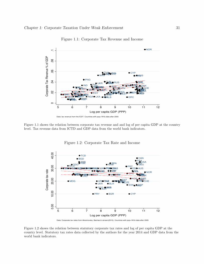
Chapter 1: Corporate Taxation Under Weak Enforcement 31
Figure 1.1: Corporate Tax Revenue and Income
ALB
ARM
AUS
AUT
BEL
BFABGD
BGR
BIH
BLR
BRACANCHE
CHLCRI
CYP
CZE
DEU
DNK
DOMEGY ESPESTETH
FINFRA
GAB
GBRGEO
GHA
GRC
GTM
HKG
HNDHRV
IND
IRL
ITAJOR
JPN
KAZ
KENKOR
LAOLKA
MAR
MDG
MLI
MNG
MOZ
MRT
MWI
MYS
NAM
NER NGA
NLD
NOR
NPL
NZL
PAK
PAN
PER
PHL
PNG
POL
PRT
PRY
RUS
SDN
SEN
SGP
SLESRB
SVN
SWESWZ
SYR
TCD
TGO
THA
TUN
TUR
TZAUGA
UKR
URYUSA
ZAF
ZMB
ZWE
0.0
2.0
4.0
6.0
8.1
Cor
pora
te T
ax R
even
ue %
of G
DP
5 6 7 8 9 10 11 12
Log per capita GDP (PPP)
Data: tax revenue from the ICDT. Countries with pop>1M & data after 2005
Figure 1.1 shows the relation between corporate tax revenue and and log of per capita GDP at the countrylevel. Tax revenue data from ICTD and GDP data from the world bank indicators.
Figure 1.2: Corporate Tax Rate and Income
ALB
ARM
AUS
AUT
BEL
BGD
BGR
BLR
BRA
CAN
CHECHL
CRI
CYP
CZE
DEU
DNK
DOM
EGY
ESP
EST
ETH
FIN
FRA
GAB
GBR
GEO
GHAGRC
GTM
HKG
HND
HRV
IND
IRL
ITA
JOR
JPN
KAZ
KEN
KORLAO
LKAMAR
MDG
MNG
MOZ
MRT
MWI
MYS
NAM
NGA
NLDNOR
NPL
NZL
PAK
PAN
PERPHLPNG
POL
PRT
PRY
RUS
SEN
SGP
SLE
SRBSVN
SWE
SWZSYR
TCD
TGO
THA
TUN
TUR
TZAUGA
UKR
URY
USA
ZAF
ZMB
ZWE
0.00
10.0
020
.00
30.0
040
.00
Cor
pora
te ta
x ra
te
5 6 7 8 9 10 11 12
Log per capita GDP (PPP)
Data: Corporate tax rates from Abramovsky, Bachas & Jensen(2015). Countries with pop>1M & data after 2005
Figure 1.2 shows the relation between statutory corporate tax rates and log of per capita GDP at thecountry level. Statutory tax rates data collected by the authors for the year 2014 and GDP data from theworld bank indicators.

Chapter 1: Corporate Taxation Under Weak Enforcement 32
Figure 1.3: Costa Rica’s Corporate Tax Schedule
0 20 40 60 80 100 120 140
10%
20%
30%
Revenue (Million crc)
Ave
rage
Tax
Rat
e
Tax Base isProfits = Revenue - Costs
T1 T2
Figure 1.3 shows the design of the corporate income tax in Costa Rica. Firms pay increasing average taxrates on their profits as a function of their revenue. When revenue exceeds the first threshold, the averagetax rate jumps from 10% to 20% and from 20% to 30% past the second threshold.
Figure 1.4: Bunching Theory
Revenue (Million crc)
Firm
Den
sity
Costs too High to bunch
Exce
ss M
ass
Missing mass
Observed density
Counterfactualdensity
y_T
Figure 1.4 displays the theoretical density distribution. Under a flat 10% tax rate the counterfactual firmdensity follows a smooth distribution. The notch induces some firms, with counterfactual revenue abovethe threshold, to reduce their revenue and bunch just below the threshold. The bunching decision is a jointfunction of the firm’s revenue distance to the threshold and costs, such that at each revenue bin past thethreshold, only firms with su�ciently low costs bunch.

Chapter 1: Corporate Taxation Under Weak Enforcement 33
Figure 1.5: Firm Density and Average Profit Margin0
500
1000
1500
2000
2500
3000
Num
ber
of F
irms
20 30 40 50 60 70 80 90 100 110 120 130 140
Revenue (Million crc)
Panel A: Firm Density
0.0
5.1
.15
.2.2
5
Ave
rage
Pro
fit M
argi
n
20 30 40 50 60 70 80 90 100 110 120 130 140
Revenue (Million crc)
Panel B: Profit Margin
Figure 1.5 presents the key patterns of the corporate tax returns, pulling together the years 2008 to 2014.Panel A shows the density of firms by revenue. Panel B displays the average profit margin by revenue,where profit margin is defined as profits over revenue. The size of the revenue bins is 575,000 CRC.

Chapter 1: Corporate Taxation Under Weak Enforcement 34
Figure 1.6: Revenue Bunching Estimation
B = 2.3 y_u = 58.3
y_l y_u
500
1000
1500
2000
2500
3000
Num
ber
of fi
rms
30 40 50 60 70 80
Revenue (Million crc)
Panel A: First threshold
B = 1.1 y_u = 107.7
y_l y_u
300
400
500
600
700
800
900
Num
ber
of fi
rms
80 90 100 110 120 130
Revenue (Million crc)
Panel B: Second threshold
Figure 1.6 displays the density of firms by revenue and fits the counterfactual distribution for the first andsecond thresholds. In the boxes on the top right, B is the excess mass as a share of the counterfactual, andyu
the revenue of the marginal buncher, obtained with the point of convergence method. Thecounterfactual is obtained from the regression of a polynomial of degree 5 (maximizes Akaike criteria), onall data points outside the [y
l
, yu
] interval. The lower bound yl
is chosen by the researchers as the revenuebin which starts exhibiting excess. The upper bound y
u
is estimated from an iterative process: startingfrom y
u
close to the threshold, we obtain the counterfactual and estimate the excess mass (B) below thethreshold and missing mass (M) above the threshold. For low y
u
, the excess mass is larger than the missingmass, B >> M . We increase y
u
until the two masses are equal, B = M .

Chapter 1: Corporate Taxation Under Weak Enforcement 35
Figure 1.7: Cost Discontinuity
y_l y_u
2030
4050
6070
Ave
rage
Cos
t (M
illio
n cr
c)
30 40 50 60 70 80
Revenue (Million crc)
Average Cost
Cost adjusted for e_y
Linear fit
Extrapolated linear fit
Panel A: First Threshold Cost by Revenue
y_l y_u
Cost jump= 2.55 M
3540
4550
55
Ave
rage
Cos
t (M
illio
n cr
c)
40 45 50 55
Revenue (Million crc)
Panel B: Cost discontinuity (zoom)
Figure 1.7 displays the average declared cost for each revenue bin around the first threshold. To estimatethe cost discontinuity at the threshold, absent revenue responses, we adjust for intensive margin revenueresponses: firms declaring revenue above the threshold reduced their declared revenue, due to the the taxrate increase. To take intensive responses into account, we horizontally shift firms’ costs proportionally tothe elasticity of revenue, estimated from bunching. For example, given an elasticity of revenue of 0.25 anda firm with revenue of 60M: revenue
counter
= 60 + ✏y,1�t
.y. dt
1�t
= 60 + 0.25 ⇤ 60 ⇤ 0.10.9 ⇡ 61.6. We linearly fit
costs by revenue, below and above the threshold. On either side, we exclude revenue bins impacted bybunching behavior. We then extrapolate the linear fits to the threshold. The resulting cost discontinuityrepresents the average increase in declared costs, for a firm at the threshold, due to an increase in the taxrate from 10 to 20%.

Chapter 1: Corporate Taxation Under Weak Enforcement 36
Figure 1.8: Linear Relation of Average Costs by Revenue
20
25
30
35
40
Avera
ge C
osts
30 35 40 45
Revenue (Million crc)
Below 1st Threshold
55
60
65
70
Avera
ge C
osts
60 65 70 75
Revenue (Million crc)
Above 1st Threshold
70
75
80
85
90
Avera
ge C
osts
80 85 90 95
Revenue (Million crc)
Below 2nd Threshold
105
110
115
120
Avera
ge C
osts
110 115 120 125
Revenue (Million crc)
Above 2nd Threshold
Average costs linear fit quadratic fit
Figure 1.8 shows the linearity of the relation between average costs and revenue. For each of the fourrevenue intervals considered (below and above the first and second threshold), we plot the linear andquadratic fits of the data. Quadratic fits are practically indistinguishable from Linear fits providingsupport to our linear extrapolation assumption.

Chapter 1: Corporate Taxation Under Weak Enforcement 37
Figure 1.9: E↵ective Tax Rate on Revenue
ATR=10% ATR=20% ATR=30%
0.0
05.0
1.0
15.0
2.0
25.0
3
Tax P
aym
ent a
s Sha
re o
f Rev
enue
20 30 40 50 60 70 80 90 100 110 120 130 140
Revenue (Million crc)
Figure 1.9 plots average tax payment as a share of revenue for revenue bins of half million CRC. The largeprofit elasticity implies that despite a 10% tax rate increase past each threshold, taxes e↵ectively paid areconstant at 1 to 1.5% of the firm’s revenue for all tax brackets.
Figure 1.10: Quartiles of Profit Margin by Revenue
0.0
1.0
2.0
3
Pro
fit m
arg
in, P
25
20 40 60 80 100 120 140
Revenue (Mil CRC)
Bottom quartile
0.0
2.0
4.0
6.0
8.1
Pro
fit m
arg
in, M
edia
n
20 40 60 80 100 120 140
Revenue (Mil CRC)
Median
0.1
.2.3
.4
Pro
fit m
arg
in, P
75
20 40 60 80 100 120 140
Revenue (Mil CRC)
Top quartile
Note: The y−axis scale is not constant across figures
Figure 1.10 shows the distribution of profit margins by revenue for each quartile within a revenue bin. Thediscontinuous step pattern observed for average profit margins is observed for all percentiles and isgenerated by an entire downwards shift of the distribution and not only by the reduced reportedprofitability of a few high profitability firms.

Chapter 1: Corporate Taxation Under Weak Enforcement 38
Figure 1.11: Industry Results
0.1
.2.3
.4
0.0
2.0
4
Agriculture
0.1
.2.3
.4
0.0
2.0
4
Manufacture
0.1
.2.3
.4
0.0
2.0
4
Construction
0.1
.2.3
.4
0.0
2.0
4
Wholesale & Motor vehicle
0.1
.2.3
.4
0.0
2.0
4
Retail
0.1
.2.3
.4
0.0
2.0
4
Hotel & restaurants
0.1
.2.3
.4
0.0
2.0
4
Transport
0.1
.2.3
.4
0.0
2.0
4
Fin. activities & equipment rental
0.1
.2.3
.4
0.0
2.0
4Real estate
0.1
.2.3
.4
0.0
2.0
4
Legal & econ. consultancies
0.1
.2.3
.4
0.0
2.0
4
Other services
0.1
.2.3
.4
0.0
2.0
4
Education & Culture
0.1
.2.3
.4
0.0
2.0
4
Health
0.1
.2.3
.4
0.0
2.0
4
Assoc. & Public admin.
0.1
.2.3
.4
0.0
2.0
4
Undetermined
Within industry density(Blue) & profit margin(Green)
Figure 1.11 presents the firm density and profit margin by revenue, separating the economy in fifteenindustries. In blue, the within industry firm density by revenue and in green the average profit margin byrevenue. We observe for all sectors a large discontinuous drop in average profit margins, while bunchingbehavior is more heterogeneous.

Chapter 1: Corporate Taxation Under Weak Enforcement 39
Figure 1.12: Excess Mass and Profit Discontinuity by Industry
Agriculture
Manufacture
Construction
Wholesale & Motor vehicleRetail
Hotel & Restaurants
Transport
Fin. ActivitiesReal Estate
Legal & Econ. consultancies
Other Services
Education & Culture
Health
Public Admin.
Undetermined
01
23
45
6Ex
cess
Mas
s
−.7 −.6 −.5 −.4 −.3 −.2 −.1 0 .1 .2Percentage Change in Profit
Figure 1.12 shows the relation between the profit margin discontinuity and excess mass by industry, at thefirst threshold.
Figure 1.13: Structural Assumption - Stable Profit Margin Distributions
01
23
45
67
Dens
ity
0 .2 .4 .6 .8
Profit margin
[−6,−8] [−8,−10]
[−10,−12] [−12,−14]
Revenue Distance to 1st Thresh. (Mil)
Panel A: Below threshold
01
23
45
67
Dens
ity
0 .2 .4 .6 .8
Profit margin
[10,12] [12,14]
[14,16] [16,18]
Revenue Distance to 1st Thresh. (Mil)
Panel B: Above threshold
Figure 1.13 shows that the distribution of profit margin is stable across revenue intervals 10 to 20% belowthe threshold (Panel A), and revenue intervals 20 to 30% above the threshold (Panel B). The legendindicates the revenue intervals to the threshold considered. We use an Epanechnikov kernel with bandwithof 0.04 across all distributions. Within each panel, we never reject the Kolmgorov-Smirnov tests, that profitmargins are sampled from populations with identical distributions across all pairs of revenue intervals.

Chapter 1: Corporate Taxation Under Weak Enforcement 40
Figure 1.14: Numerical Estimation of Bunching Behavior0
500
1000
1500
Num
ber o
f Firm
s
0 2 4 6 8 10
Revenue Distance to 1st Threshold (Million crc)
Counterfactual Density e_y=0.03
e_y=0.14 e_y=0.33
Panel A: Revenue Elasticity Scenarios
050
010
0015
00
Num
ber o
f Firm
s
0 2 4 6 8 10
Revenue Distance to 1st Threshold (Million crc)
Bunching Firms Counter. Density e_y=0.22
Panel B: Estimated Revenue Easticity
Figure 1.14 displays the results from the numerical model-based estimation, when assuming a jointcounterfactual distribution of revenue and costs and that bunchers cost response correspond to the averagecost response. For a given revenue elasticity, e
y
and cost elasticity, ec
, the area between the counterfactualdensity and the curves represents the number of bunching firms. In panel A, we display the profile of thesecurves for several values of the revenue elasticity. Panel B, displays the result for the last iteration: thenumber of estimated bunchers equals the observed bunchers and the revenue and cost elasticity are inequilibrium.

Chapter 1: Corporate Taxation Under Weak Enforcement 41
Figure 1.15: Dynamic Firm Behavior by Tax Bracket−5
−4−3
−2−1
01
23
45
Diffe
renc
e in
prof
it mar
gin b
etwe
en ye
ar t
and
t+1
(%)
10% at t 20% at t 30% at t
Dynamic behavior of firms by tax group
10% at t+1 20% at t+1 30% at t+1
Figure 1.15 shows the average change in firms’ profit margins between year t and t+1 as a function of theirtax brackets in year t and t+1. On the one hand, firms remaining within their initial tax bracket hardlychange reported profits. On the other hand, firms jumping to higher tax brackets drop their profit marginsand symmetrically firms falling to lower tax bracket increase their profit margins.
Figure 1.16: Profit Margin Change for Growing Firms
−.04
−.02
0.0
2.0
4
Chan
ge in
Pro
fit M
argin
(t=0
to t=
1)
−11−10 −9 −8 −7 −6 −5 −4 −3 −2 −1 0 1 2 3
Distance from Threshold (2 Mill CRC bins) at t=0
Firms with 3−5 Million growth in revenue
−.06
−.04
−.02
0.0
2.0
4
Chan
ge in
Pro
fit M
argin
(t=0
to t=
1)
−11−10 −9 −8 −7 −6 −5 −4 −3 −2 −1 0 1 2 3
Distance from Threshold (2 Mill CRC bins) at t=0
Firms with 7−9 Million growth in revenue
Figure 1.16 plots the average change in firms’ profit margins between year t and t+1 for the subset of firmswho’s revenue grew by 3 to 5 Million (Left Panel) and by 7-9 Million (Right Panel). This figure visuallyshows the di↵erence in di↵erences across the group of firms that jumped past the threshold versus the firmsthat stayed within the same tax bracket, while controlling for revenue growth.

Chapter 1: Corporate Taxation Under Weak Enforcement 42
Figure 1.17: Correction Letters by Revenue (2012).2
.25
.3.3
5.4
.45
% o
f Firm
s re
ceivi
ng le
tter
30 40 50 60 70 80 90 100
Revenue (Million CRC)
Ratio Fitted line excl. dotted area 95% CI
Figure 1.17 displays the percentage of firms receiving correction letters due to an inconsistency in their taxdeclaration or a discrepancy with third party information. Bunching firms are significantly more likely toreceive a letter showing an inconsistency with their third-party reports. Each revenue bin represents a 2Million CRC interval. The fitted line excludes the revenue intervals impacted by the bunching selection.
Figure 1.18: Share of Subsidiaries by Revenue
disc_T1 = −.39 (.26)buncher = .31 (.34)
02
46
8
Shar
e of
Sub
sidi
ary
firm
s (%
of t
otal
)
−20 −10 0 10 20
Revenue distance to threshold (Mil crc)
1st Threshold
disc_T2 = −.14 (.39)buncher = .83 (.33)
02
46
8
Shar
e of
Sub
sidi
ary
firm
s (%
of t
otal
)
−20 −10 0 10 20
Revenue distance to threshold (Mil crc)
2nd Threshold
Figure 1.18 shows the percentage of firms that are subsidiaries of a larger firm, by revenue. The lack ofdiscontinuity in the share of subsidiaries around the thresholds empirically shows that firm division toevade taxes is not a first order strategy.

Chapter 1: Corporate Taxation Under Weak Enforcement 43
Figure 1.19: Employment and Wage Bill by Revenue
disc_T1 = −.035 (.053)buncher = −.016 (.059)
01
23
45
67
8A
vera
ge e
mplo
ym
ent
−20 −10 0 10 20Revenue distance to threshold (Million CRC)
Employment, 1st Threshold
disc_T2 = −.122 (.089)buncher = −.028 (.101)
01
23
45
67
8A
vera
ge e
mplo
ym
ent
−20 −10 0 10 20Revenue distance to threshold (Million CRC)
Employment, 2nd Threshold
disc_T1 = .015 (.01)buncher = .011 (.015)
0.0
5.1
.15
.2.2
5.3
Wage b
ill share
of re
venue
−20 −10 0 10 20Revenue distance to threshold (Million CRC)
Wage bill, 1st Threshold
disc_T2 = 0 (.006)buncher = −.016 (.006)
0.0
5.1
.15
.2.2
5.3
Avg w
age b
ill (M
il C
RC
)
−20 −10 0 10 20Revenue distance to threshold (Million CRC)
Wage bill, 2nd Threshold
Figure 1.19 shows the average number of employees and wage bill by revenue around the first and secondthresholds. The data is obtained from a merge of social security records with corporate income tax returns.We display the coe�cient and standard errors from the discontinuity regression at the threshold and thedummy coe�cient for firms in the bunching interval.

Chapter 1: Corporate Taxation Under Weak Enforcement 44
Figure 1.20: Cost Categories Breakdown0
.1.2
.3.4
.5.6
.7
Cost
as a
shar
e of
reve
nue
30 40 50 60 70 80
Revenue (Million crc)
Admin and Operations Materials Other (Depr., Fin.)
Cost Category
Figure 1.20 shows the cost discontinuity by revenue, broken down into the three main cost categoriesreported on the tax returns (“Formulario D101”). Each cost category is displayed as a percentage ofrevenue. The five categories on the corporate tax returns are: administrative and operational costs,material and production costs, depreciation, interest deductions and other costs and we group the laterthree categories together.
Figure 1.21: Worldwide Corporate Tax Systems by Income Quintiles
0.2
.4.6
.81
Shar
e of
cou
ntrie
s
Lower−Income Middle−Income OECD
Note: Authors’ computation based on data collected by Abramovsky, Bachas & Jensen (2015)
Presumptive tax Revenue dependent rate Flat or increasing MTR
Corporate Income Tax types
Figure 1.21 shows the worldwide distribution of corporate income tax types, dividing country into threeincome groups. The sample contains 120 countries, with data on corporate incomes tax types collectedfrom international tax guides by Abramovsky, Bachas, and Jensen 2015 and per-capita income data fromthe Penn Tables. Presumptive tax systems are very common for low-income countries, while CIT withrevenue dependent rate, such as Costa Rica’s, are sometimes used in middle-income countries. In richcountries, the corporate income is almost always taxed at a flat or increasing marginal rate.

Chap
ter1:
Corp
orateTaxation
Under
Weak
Enforcem
ent45
Table 1.1: Summary of Estimates and Assumptions
Method Estimation strategy Elasticity Bound Assumptions
Reduced form
Step 1 ! ✏y
Bunching: empirical ✏y,1�⌧
= 0.33 Upper bound: Counterfactual firm density
+ point of convergence ✏y
of marginal buncher by revenue is regular
Step 2 ! ✏c
(✏y
) Cost discontinuity ✏c,1�⌧
= �0.55 Lower bound: Linear cost extrapolation
+adjustment for ✏
y
! is correct✏c
negative relation with ✏y
Step 3 ! ✏⇡
(✏y
, ✏c
) d⇡ = dy � dc ✏⇡,1�⌧
= 4.93
Added structure Profit margin distribution of firms with revenue 10% below the threshold would apply to firmswith revenue just above the threshold absent the tax change
With dc = dc
Step 1 ! ✏y
(✏c
) Bunching: numerical ✏y,1�⌧
= 0.22 Bunchers would have dc = dc
m Iterateelasticity ✏
y
if not bunching
Step 2 ! ✏c
(✏y
) Cost discontinuity ✏c,1�⌧
= �0.65
+
Step 3 ! ✏⇡
(✏y
, ✏c
) d⇡ = dy � dc ✏⇡,1�⌧
= 4.90
With dc = 0
Step 1 ! ✏y
Bunching: numerical ✏y,1�⌧
= 0.095 Lower bound: Bunchers would have dc = 0
+ elasticity ✏y
Assumption dc=0 if not bunching
Step 2 ! ✏c
Cost discontinuity ✏c,1�⌧
= �0.79 Upper bound:
+ ✏c
negative relation with ✏y
Step 3 ! ✏⇡
(✏y
, ✏c
) d⇡ = dy � dc ✏⇡,1�⌧
= 4.90

Chapter 1: Corporate Taxation Under Weak Enforcement 46
Table 1.2: Robustness of Bunching Estimates
Panel A: Varying the order of the PolynomialOrder of Polynomial 4 5 6
First ThresholdB 2.4 2.2 2.2yu
59.4 58.3 58.8✏y,1�⌧
0.41 0.33 0.36
Second ThresholdB 1.1 1.1 1.1yu
108.3 107.7 107.7✏y,1�⌧
0.10 0.08 0.08
Panel B: Varying the excluded zone, yl
Number of excluded bins 6 7 8
First ThresholdB 2.0 2.2 2.3yu
57.1 58.3 58.3✏y,1�⌧
0.25 0.33 0.33
Second ThresholdB 1.1 1.1 1.0yu
107.1 107.7 106.6✏y,1�⌧
0.07 0.08 0.06
Table 1.2 shows under di↵erent scenarios the estimates of the excess mass B, the revenue of the marginalbuncher y
u
and the resulting revenue elasticity ✏y,1�⌧
. Panel A varies the order of the polynomial andPanel B the number of excluded bins on the lower side, which corresponds to y
u
.

Chapter 1: Corporate Taxation Under Weak Enforcement 47
Table 1.3: Cost on Revenue Distance to Threshold Relation
1st Threshold 2nd Threshold
Cost Cost(revenue adjust.) Cost Cost(revenue adjust.)
Jump in cost � 4.203** 2.548** 2.223** 1.277**(0.212) (0.226) (0.416) (0.432)
Slope below T. �1 0.834** 0.834** 0.933** 0.933**(0.010) (0.010) (0.015) (0.015)
Slope change above T. �2 0.103** 0.069** 0.017 0.008(0.014) (0.014) (0.026) (0.026)
Intercept ↵ 41.971 41.971 93.863 93.863Observations 80 80 80 80
% Jump in Cost �
↵
+10.01% +6.07% +2.37% +1.36%
Table (1.3) shows the results from the regression of average costs by revenue on revenue distance to thethreshold, estimated from equation (1.14). For each threshold we report the discontinuity in cost � withand without the revenue adjustment. The revenue adjustment holds revenue responses above the thresholdconstant, using the revenue elasticity estimated with bunching, such that the discontinuity in the cost torevenue relation, after adjustment, only identifies cost responses: the results from column (2) & (4) are ourmain estimate of the cost discontinuity. An observation is a revenue bin of 0.575 Million Colones. Standarderrors are shown in parentheses and stars indicate statistical significance level. *=5% level, **=1% level.

Chapter 1: Corporate Taxation Under Weak Enforcement 48
Table 1.4: Alternative Models for Cost Discontinuity by Revenue
1st Threshold 2nd Threshold
Model Specification (1) (2) (3) (4) (5) (6) (7) (8)
Narrow WideFalling ✏
y
QuadraticNarrow Wide
Falling ✏y
QuadraticWindow Window Window Window
Jump in cost � 2.688** 2.465** 2.326** 3.804** 1.389* .85* 1.277** 3.113**(.249) (.204) (.246) (.583) (.591) (.392) (.432) (.726)
Slope below T. .823** .841** .834** .603** .924** .944** .933** .821**(.012) (.007) (.009) (.089) (.02) (.012) (.015) (.078)
� Slope above T. .079** .063** .107** .297** .014 .018 .008 -.052(.017) (.011) (.014) (.092) (.042) (.021) (.026) (.098)
Quadratic below T. -.009** -.004(.003) (.003)
� Quadratic above T. .009** .01**(.003) (.003)
Intercept, ↵ 41.86 42.046 41.971 40.682 93.777 93.99 93.863 93.217
Observations 70 90 80 80 70 90 80 80
% Jump in Cost �
↵
+6.42% +5.86% +5.54% +9.34% +1.48% +0.91% +1.36% +3.36%
Table 1.4 shows the regressions of average costs by revenue on revenue for di↵erent model specifications.The parameter of interest is the jump in declared costs at the threshold, �, from Equation (1.14).Compared to the main specification of Table (1.3), Rows (1)-(2) & (5)-(6) vary the revenue interval overwhich the line is fitted. Rows (3) & (7) assume that the revenue elasticity is falling with revenue, at thespeed estimated between the first and second threshold. Rows (4) & (8) assume a quadratic fit instead of alinear fit. An observation is a revenue bin of 0.575 Million Colones. Standard errors are shown inparentheses and stars indicate statistical significance level. *=5% level, **=1% level.
Table 1.5: Elasticity Estimates - Point of Convergence
Parameters Elasticity Threshold jumpy⇤ dy⇤ 1� ⌧0 ⌧ ⇤ Revenue Cost Profit �y �c �⇡
50 8.3** 0.9 0.55 0.33** -0.55** 4.93** -1.84 2.55 -4.39(1.3) (0.07) (0.06) (0.28)
100.5 7.2** 0.8 0.77 0.08* -0.11* 2.92** -0.99 1.27 -2.26(1.8) (0.04) (0.05) (0.71)
Table (1.5) shows the elasticity estimates obtained with the point of convergence method. Cost elasticitiesare estimated with the threshold discontinuity, holding constant revenue responses. The profit elasticitycombines revenue and cost responses. Standard errors are obtained through 1,000 bootstrap iterations. y⇤
is the revenue threshold in Million CRC and dy⇤ is the revenue response of the marginal buncher estimatedwith bunching. 1� ⌧0 is the average tax rate below each threshold and ⌧⇤ is the implicit marginal tax ratefaced by the marginal buncher. Standard errors are shown in parentheses and stars indicate statisticalsignificance level. *=5% level, **=1% level.

Chapter 1: Corporate Taxation Under Weak Enforcement 49
Table 1.6: Model-Based Numerical Estimation: Iteration Steps
Iteration Revenue Elasticity Cost Jump Cost ElasticityStep ✏
y,1�t
dc ✏c,1�t
1 0.33 2.55 -0.552 0.17 3.25 -0.703 0.26 2.83 -0.614 0.19 3.17 -0.685 0.24 2.93 -0.636 0.21 3.07 -0.667 0.23 2.98 -0.64
Final 0.22 3.02 -0.65
Table 1.6 shows the iteration steps of the model-based numerical bunching estimation. With acounterfactual firm density by revenue and a counterfactual profit margin distribution, the methodnumerically estimates the number of bunching firms as a joint function of their revenue distance to thethreshold and costs. Step 1 uses as initial values the revenue and cost elasticity from section 1.3. Underthose parameters the revenue elasticity of Step 2 is su�cient such that the number of bunchers equal thatof the excess mass. With this new revenue elasticity we re-estimate the cost elasticity using thediscontinuity method of 1.3. We iterate this procedure until we find the fixed point at which the revenueand cost elasticities are consistent with the observed bunching behavior.
Table 1.7: Industry Level Results 1st Threshold
Profit Margin (%) Bunching # FirmsSector Drop Base % Drop Excess Mass Total % Below T1
Agriculture -4.1 8.4 -48.8 1.95 33,095 59.5Manufacture -3.2 6.8 -47.1 2.34 34,799 45.4Construction -5.2 9.5 -54.7 3.17 26,410 51Wholesale & Motor Vehicle -3.5 7 -50 1.11 63,544 45.1Retail -4.9 8.5 -57.6 1.17 100,552 47.9Hotel & Restaurants -3.5 7 -50 1.41 21,483 49Transport -4.1 9.9 -41.4 2 36,294 54.7Financial Activities -10.3 21.8 -47.2 3.93 26,366 71.9Real Estate -13 36.4 -35.7 4.05 91,525 85.1Legal & Econ. Consultants -9.5 17 -55.9 6.27 64,617 73.3Other Services -9.3 14.6 -63.7 4.37 37,091 69.3Education & Culture -1.3 5.8 -22.4 2.64 14,228 56.8Health -8.4 17.1 -49.1 3.23 19,611 65.2NGO & Public Admin. .8 28.1 2.8 -.19 10,608 68.8Undetermined -9.6 19.9 -48.2 3.66 36,044 80.8

Chapter 1: Corporate Taxation Under Weak Enforcement 50
Table 1.8: Dynamic Firm Behavior
Profit Margin1st Threshold 2nd Threshold
Revenue (Million CRC) 0.0115** 0.0071*(0.0039) (0.0029)
Higher Tax Bracket -3.06** -0.86**(0.17) (0.14)
Buncher (Narrow) 1.56** 0.46**(0.27) (0.14)
Bunching (Broad) 0.84** 0.60*(0.20) (0.27)
Above threshold (Narrow) -0.33 -0.10(0.18) (0.17)
Above threshold (Broad) -0.12 0.02(0.11) (0.10)
Constant (Avg across years) 14.63 5.62
Firm & Year fixed e↵ects YES YES
Observations 289,744 88,493
All firms with revenue in a 70 Million CRC window centered around the thresholds are included in thesample. Profit margin is defined as profit over revenue. The Bunching and above threshold are dummiesfor declaring revenue in the intervals around the threshold. Bunching narrow is defined as the havingrevenue in the half Million interval below the threshold. Bunching wide as having revenue between 4 and0.5 Million below the threshold. Above threshold narrow is defined as having revenue between 0 to 3Million above the threshold and wide as having revenue 3 to 9M above threshold. Standard errors areshown in parentheses and stars indicate statistical significance level. *=5% level, **=1% level.
Table 1.9: Revenue Shifting at the End of the Fiscal Year
Dependent Variable: Monthly Revenue (Million CRC)All firms CIT rev. = sales tax rev.
(1) (2) (3) (4) (5) (6) (7) (8)
Buncher*Sept 0.10 0.05 -0.17 0.30**(0.12) (0.09) (0.32) (0.07)
Buncher*Oct -0.02 -0.21 -0.62 -0.12(0.12) (0.13) (0.48) (0.10)
Firm FE NO YES NO YES NO YES NO YES
Observations 596,705 596,705 596,705 596,705 115,649 115,649 115,649 115,649
Table 1.9 tests for revenue shifting at the end of the fiscal year using the revenue declared for the monthlysales tax payment. Robust standard errors are shown in parentheses and stars indicate statisticalsignificance level. *=5% level, **=1% level.
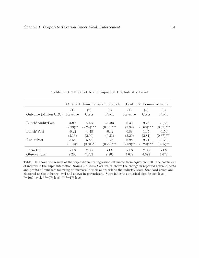
Chapter 1: Corporate Taxation Under Weak Enforcement 51
Table 1.10: Threat of Audit Impact at the Industry Level
Control 1: firms too small to bunch Control 2: Dominated firms
(1) (2) (3) (4) (5) (6)Outcome (Million CRC) Revenue Costs Profit Revenue Costs Profit
Bunch*Audit*Post 4.87 6.43 -1.23 6.30 9.76 -1,68(2.39)** (2,24)*** (0.33)*** (3.99) (3.63)*** (0.57)***
Bunch*Post -0.22 -0.48 -0.42 0.88 1.35 -1.50(2.13) (2.00) (0.31) (3.20) (2.81) (0.37)***
Audit*Post 5.55 5.88 -1.25 6.98 9.21 -1.70(3.10)* (3.01)* (0.29)*** (2.89)** (3.29)*** (0.65)**
Firm FE YES YES YES YES YES YESObservations 7,203 7,203 7,203 4,672 4,672 4,672
Table 1.10 shows the results of the triple di↵erence regression estimated from equation 1.20. The coe�cientof interest is the triple interaction Bunch ⇤Audit ⇤ Post which shows the change in reported revenue, costsand profits of bunchers following an increase in their audit risk at the industry level. Standard errors areclustered at the industry level and shown in parentheses. Stars indicate statistical significance level.*=10% level, **=5% level, ***=1% level.

52
Chapter 2
An Empirical Test of InformationTrails: Do Firm Finance and SizeMatter for Tax Collection?
with Anders Jensen
2.1 Introduction
Governments enforcing taxes are constrained by the stock and flows of information on trans-actions in the economy. Third-party reporting, verifiable paper trails, and whistle-blowingmechanisms have been shown empirically to create important information flows that facili-tate tax enforcement (Kopczuk and Slemrod 2006, Kleven et al. 2011b, Kumler, Verhoogen,and Frias 2012, Pomeranz 2015b, Carillo, Pomeranz, and Singhal 2015).In the theoretical literature, two settings in particular have been emphasized as powerfulgenerators of tax-relevant information: the firm’s interaction with the financial system andthe firm’s worker size. The financial trail is based on the insight that when accessing formalbanking firms generate a paper trail of information, often including financial statements andlists of customers Gordon and Li (2009b). If this financial information trail is shared by thebank with the tax authority, it may constitute the basis for stronger tax enforcement onfinancially connected firms.The firm-size information trail is related to the idea that firms with more employees are morecomplex and thus require more accurate book-keeping (Kleven, Kreiner, and Saez 2016). Inthe hands of a tax auditor, such book-keeping constitutes the paper trail necessary to en-force tax liability. Larger firms can still evade by keeping parallel books (one for their ownuse, one for the tax authority) but evasion will be more costly and collusion to under-reportactivities between employer and employees more likely to break down. This could be due

Chapter 2: An Empirical Test of Information Trails 53
either to random shocks that reveal the true internal records or to whistle-blowing.Despite the importance of the worker-size and the financial information trails in the theoret-ical literature no studies has tested their empirical relevance. We provide the first empiricaltest to study whether larger-sized firms and more financially externally reliant firms facehigher tax inspection and comply more with sales taxes. To motivate the empirical speci-fication, we formulate a reduced-form model in which firm behavior generates informationtrails that tax authorities can use to enforce tax collection.We use the World Bank Enterprise Surveys (WBES) 2002-2010, a firm level survey withinformation on firm-size, external financial reliance, tax inspection and reported sales taxcompliance for 108,000 firms in 79 countries. In Fig.1, pooling all countries together, wegroup firms in twenty equal-sized groups (vingtiles) of firm-size distribution, and plot meantax inspection and sales tax compliance across the twenty vingtiles. Enforcement and com-pliance clearly increase monotonically by firm-size. In Fig.2 we construct the same graph,with twenty quantiles of external financial reliance. The upwards-sloping relationship ismuch less clear, both with regards tax inspection and sales tax compliance. These figuressummarize a general trend in all our regressions results: we systematically uncover a strongpositive e↵ect of the firm-size information trail on tax inspection and sales tax complianceand an insignificant e↵ect of the external finance trail.In the regression setting, we isolate exogenous demand-driven variation in external fundingand firm-size at the industry-level, by adopting an identification strategy related to Rajanand Zingales (1998), (RZ hereafter). The identification strategy consists in predicting thesize-ranks and the external finance-ranks of an industry within a WBES country from thesize and external finance rankings of the same set of industries in the U.S. This out-of-sampleextrapolation technique relies on the assumption that the labor and finance markets of theU.S. are relatively undistorted and thus that the ranking of industries in external relianceand number of workers in the U.S. reflects “benchmark” technological di↵erences in demandfor labour and funding inputs. The first stage shows the extent to which US industry-ranksin firm-size and funding choice explain the WBES countries’ corresponding industry-ranks.As RZ did not have data on external funding for firms in developing countries, we believeour study is the first to test the hypotheses of industry-specific country-invariant demandtechnologies for finance and firm-size in a large dataset of both developed and developingcountries. We find strong evidence in favor of the industry-specific technology for workers,but weak evidence in the case of financial external reliance. In a double IV specification,which simultaneously instruments external reliance rank and firm-size rank by the U.S. rank-ings in external reliance and the US firm-size, we uncover strong e↵ects for the worker-sizetrail on both tax inspection and sales tax compliance, but no discernible impact of externalreliance. Finally, we study the impact of the information trails on tax evasion through thetax inspection channel. The exclusion restriction is less strong in this setting, as informationtrails could impact tax compliance through other channels than solely tax inspection. Withthat caveat in mind, we find that exogenous changes in firm-size and external reliance predictlarge positive changes to tax compliance through increased tax enforcement. These resultsspeak to the importance of information trails and third party information in understanding

Chapter 2: An Empirical Test of Information Trails 54
firm level tax compliance behavior. The results also relate to the revenue versus productione�ciency trade-o↵ the tax authority faces when choosing enforcement instruments. On theone hand, the tax administration may consciously choose to leave aside relevant informationtrails generated from firm-size and external funding, since any enforcement based on firmsize and funding will distort the firm input choices and generate socially costly productionine�ciencies. On the other hand, using the information trails would help to maximize rev-enue for a given amount of enforcement e↵ort: tax collection yield will be higher for theinformation-intensive firms since their paper trails allow the discovery of more evaded taxes.Empirically we find a significant firm-size e↵ect on the probability of tax inspection, suggest-ing tax administrations do actively levy the size-information trail via targeted enforcementon larger firms. We also find that tax compliance increases significantly when due to size-based enforcement, which suggests that levying the firm-size information trail generates largetax revenue returns.The non-results concerning the financial trail are interesting in their own right. The insignif-icance in all regressions could point to the lack of willingness to use financial informationby tax administrations or to the lack of access to such information. Despite an importantpush for the availability of bank information to tax authorities (OECD 2000, 2006) banksecrecy laws have often prevented significant improvements. In many countries, even in thecase of an audit, accessing bank information can be long and tedious and typically requiresthe signature of a judge.This paper contributes to the literature focusing on the importance of administrations’ infor-mation constrains in understanding tax enforcement and tax structure policy. Brockmeyeret al. (2015) study the minimum tax scheme in Pakistan where firms are taxed either onprofits or turnover depending on whichever liability is larger. The authors show that thisproduction ine�cient policy can be rationalized by revenue-e�ciency considerations, sinceit is typically harder to evade on the broader turnover tax base than on the profit tax base.Wingender (2008) tests of the relation between finance and evasion at the industry level,using an empirical strategy related to ours, uncovers a much larger impact of the finance in-formation trail than we do. Other information trails have also been discussed. For example,Pomeranz (2015b) studies the paper trail generated by VAT payments among firms in Chile.She shows that an audit threat to a firm producing at the end of the supply chain a↵ects taxpayments for the whole chain of suppliers. In addition she shows that firms already coveredby a paper trail are not a↵ected by the audit threat. She concludes that the VAT chain actsas a substitute for the paper trail in case of an audit. Artavanis, Morse, and Tsoutsoura(2012) show that a large Greek bank had informally embedded into its credit models totalincome instead of reported income. However, the authors argue that the lack of tax enforce-ment does not arise because of a lack of information but because of a lack of political will.In this case the information trail is left on the side, not for production-e�ciency reasons, butdue to political factors. Finally, Besley and Persson (2013b) develop a series of models whichstudy the government’s choice of investment in tax capacity, recognizing the practical limitsimposed on administration policy, including information constraints and political instability.Section 2 outlines an industry-representative firm model of external reliance, firm-size, tax

Chapter 2: An Empirical Test of Information Trails 55
enforcement and tax compliance, and derives the two sets of empirical predictions. Section3 discusses the data and the identification strategy. Section 4 presents the results for taxinspection and sales tax evasion and then performs robustness checks. Section 5 concludes.
2.2 Theory
Industry-representative firm specification
In order to study the relationship between information trails and tax under-reporting, wemodel the reduced-form interactions between access to external funds and tax enforcementon the one hand, and between firm-size and tax enforcement on the other hand.
Number of WorkersThe number of workers channel, formalized by Kleven, Kreiner, and Saez (2016), high-lights random shocks and whistle blowing as two mechanisms which could reveal the truebusiness records to the tax authority. The model generates a critical threshold firm-size,N, below which full evasion can be the optimal strategy. Further, the optimal amount ofunder-reporting on the intensive margin will be decreasing in N above the threshold: in thewhistle-blowing case, the reward to the whistle blower will be a share of total uncovered rev-enue, which is increasing in the size of the firm; in the random shocks case, the probabilitythat any employee reveals the true, internal records, is also increasing in the total numberof workers employed.
External Finance RelianceThe second information channel is generated by a firm’s interaction with the financial mar-kets. The important distinction is between the use of internal and external sources of funding,where the latter is characterized to generate an information trail on firm’s real activities. Wemodel the choice of internal and external cash flow based on Kaplan and Zingales (1997),a workhorse model in the finance literature. In a one-period setting, a firm chooses a levelof investment W to maximize (net-of-tax) profits. Any investment W can be financed withinternal and with external funds, denoted respectively I and E: W ⌘ I + E. The cost ofinternal funds is its opportunity cost in capital markets, which we normalize to 1. Thereexists a wedge, r, is between the firm’s internal and external cost of funds: r � 1. This wedgecould arise due to information or agency problems, which are passed on as costs to the firm.Investment financed internally is limited by the upper bound of available internal funds, I.The firm should therefore use external finance only once it has exhausted its internal fundsand reached the I limit.
Formal SettingOur model incorporates the internal and external funding choice and number of workerschoice into a standard representative-firm setting of under-reporting Chetty (2009b). Itmodels the firms tax-gain benefit of evasion e weighted against the evasion cost c(e). Later

Chapter 2: An Empirical Test of Information Trails 56
in the text we discuss some possible functional forms for c(e). Under convexity of c(e) therewill be an interior solution for evasion e.Based on our above discussion, and a novel feature to this type of reduced-form evasion-costmodels, we model the probability and cost of getting detected c(e;E;N) as increasing in thelevel of evasion e; in the amount of external funds E; and in the number of workers N weaklyabove the threshold N . The industry-representative firm faces the optimization problem:
max{I,E,N,e}
(1� t) (f(W,N)� e) + e� c�e, E, 1
�N � N
�·N
�� (rE + I)� wN (2.1)
subject to W = I + E I I e f (W,N) We define two empirical variables directlyobservable in the data and which will allow us to derive the empirical predictions:
• ↵ is external finance reliance, the share of a firm’s finance that is not met by internalfunds: ↵ = 1 � I
W
= E
E+I
. This is equivalent to the Rajan and Zingales empiricalmeasure of external financial reliance.
• � is the share of production reported for tax purposes: � = f(W,N)�e
f(W,N) .
Given the above structure, we can characterize the optimal choice of internal and externalfunds, number of workers, and evasion. The representative firm makes optimal choices basedon three first-order conditions, which are characterized by
FOC wrt e: t = ce
(e, E,N) (2.2)
FOC wrt E: (1� t)fW
(W,N) = r + cE
(e, E,N) (2.3)
FOC wrt N : (1� t)fN
(W,N) = w + cN
(e, E,N) (2.4)
Modeling the probability of tax inspection
The reduced-form evasion-cost c(e, E,N) contains the first central prediction of our study,namely that firms with more workers and with more external finance face higher tax enforce-ment. There are a number of distinct ways to model these enforcement information trails.One possibility is to specify a form for c(·) as the expected monetary loss under a tax audit,such as
c (e, E,N) = p (E,N) · (✓e) (2.5)
where p (E,N) is the probability a firm will receive a tax inspection - assumed to be in-dependent of evasion - and ✓ is the amount of evaded taxes that have to be paid in fines.Under this formulation, a firm which is perfectly compliant (e = 0) faces no compliance-cost,independently of how large and externally reliant it is. On the other hand, it may be thatlarger and more externally dependent firms face higher administrative compliance costs sim-ply from the time spent dealing with tax inspectors, such that c(0, E,N) > 0. This couldbe modeled by introducing an firm administrative cost of compliance ', such that:
c (e, E,N ;') = p (E,N) · ('+ ✓e) (2.6)

Chapter 2: An Empirical Test of Information Trails 57
Finally, the amount evaded can enter directly the probability of tax inspection, p (e, E,N),so that evading is more costly both because detection is more likely and because fines arelarger.One policy that a large number of administrations have followed to manage enforcement oftaxes on subsets of the tax-payer population is the establishment of special dedicated units,usually refereed to as Large Taxpayer Units (LTU hereafter). A firm’s inclusion in the LTUimplies an increase in the auditing probability and intensity, corresponding to a discreteupwards jump of p(·) in our model. As anecdotal policy-evidence to support modelingp = p (N), firm size N seems to constitute one of the main criteria to assign a firm tothe LTU. Pooled survey responses from administrative revenue authorities in 67 countries1
indicate that a threshold criteria in terms of number of employees is amongst the 6 mostcommon criteria for allocating a firm to the country LTU.2 In both Denmark and the UnitedKingdom a firm is assigned to the LTU once it employs in excess of 250 people; in Ghana,the threshold lies at 500, while in Sweden it is at 800; in Lithuania, allocation to the LTUis based on jointly meeting the criteria of 10+ employees and large sales revenue. Othercountries seem in practice to also target audits based on size. Goyette (2012) shows usingfirm-level data in Uganda that sales tax audits are e↵ectively based on number of employeesrather than the o�cial cut-o↵ rule which is in terms of sales. In the Finnish setting, Harju,Kosonen, and Ropponen (2014) discuss how the desk audit inspection probability for VATreturns is increasing in size for labor intensive firms. Similarly information on finance isused to select audit cases. The World Bank Risk-based tax audits report discusses thecase of Turkey which automatically cross checks VAT receipts with credit card information(Risk-Based Tax Audits: Approaches and Country Experiences 2011).
Empirical predictions of the model
There are two sets of empirical testable implications that the model delivers. The firstconcerns the relationship between tax inspection probability and the firm information trails,E and N .
Empirical prediction (1)The industry-representative firm tax inspection probability is increasing in firm-size and theamount of external funds
@p (E,N)
@N� 0 and
@p (E,N)
@E� 0 (2.7)
The positive derivative of the tax inspection probability with respect to the two informationtrails is motivated by the discussions in Section 2.1. In the case where N and E are chosen as
1Survey answers provided in Economic Development and Co-Operation (2013), totaling 52 surveyedcountries, and the International Tax Dialogue Information Series (2010), totaling 15 Sub-Saharan Africancountries.
2Other criteria cited include annual gross turnover; potential revenue contribution of the firm; size ofassets; and significant international business activity.

Chapter 2: An Empirical Test of Information Trails 58
interior solutions (i.e. N > N and E > 0), the first-order conditions (2)� (3)� (4) allow usto directly derive the second set of empirical predictions of our model. Supposing some formof underlying heterogeneity cause some firms to optimally choose higher levels of fundingand size, this will impact the firm’s compliance decision towards larger reliance on externalfinancing, ↵, and towards an increase in the optimal size of the firm, N ; these changes leadto higher tax-compliance, partly through increased tax inspection intensity. Formally
Empirical prediction (2)An exogenous increase in firm-demand for labor input causes sales tax compliance to increasein general
@�
@N� 0 (2.8)
and in particular through the channel of tax inspection
@�
@p (E,N)
@p (E,N)
@N� 0 (2.9)
Similarly, the total impact of an exogenous increase in firm reliance on external finance isfor sales tax compliance to increase
@�
@↵� 0 (2.10)
and a specific channel is through increased tax inspection
@�
@p (E,N)
@p (E,N)
@E� 0 (2.11)
In our empirical setting we will try to isolate exogenous changes in demand for labor andexternal finance input which should drive sales tax compliance through the informationtrails and the change to the cost of evasion: these are the direct tests (8) and (10). But wealso provide the empirical tests for the impact of information trails on sales tax compliancethrough changes in tax inspection probability, given by (9) and (11). In both empiricalpredictions, we simply assume that there exists heterogeneity at the industry-level causingvariation in input demands for size and external funding. One way to model this is tosuppose that there exists an industry-specific productivity-parameter ✓
i
, and that industriesdi↵er in the following sense
✓i
> ✓j
) fW
(W,N ; ✓i
) > fW
(W,N ; ✓j
) andfN
(W,N ; ✓i
) > fN
(W,N ; ✓j
) (2.12)
In the empirical exercise, we will treat di↵erences in demand for labor and external reliancebetween two U.S. industries i and j as reflective of underlying technological di↵erences.

Chapter 2: An Empirical Test of Information Trails 59
2.3 Data and Identification Strategy
Data description
Throughout the analysis the unit of observation is a country-industry, where industries areclassified using the ISIC 3 digit methodology, produced by the U.N. Statistics Division.The World Bank Enterprise Survey is the primary data source: it is a firm level surveycollected by the World bank between 2002 and 2010 in more than a hundred countries.To our knowledge this is the only standardized firm data set spanning countries across thedevelopment spectrum. Since the survey was clearly administered by a third party not relatedto the government or the statistical o�ce it could ask unique questions on tax behavior andcorruption.We rely on two data sources to construct our instrumental variables: the Compustat databaseof publicly listed firms in the U.S. and the U.S. Bureau of Labour Statistics Quarterly Censusof Employment and Wages. The final sample is 2597 country-ISIC3 observations from 77countries.3
Tax inspection and tax compliance
To operationalize a measure of tax enforcement, we use the firm’s reported answer to thequestion: “Total days spent with o�cials from: tax inspectorate.” In particular we con-structed a tax inspection dummy equals to one if the firm has been visited for at least oneday by tax auditors. This proxies for the extensive margin of tax inspection. The industry-average tax inspection probability is .71, with a standard deviation of .35. This is themeasure of tax enforcement which we used to produce Figs.1-2 in the introduction. In , wealso report the results from the ’intensive margin’ measure of total number of days. Theseresults using the ’intensive margin’ number of days visited by tax inspectors are discussedin Section 4.3.4
In a second stage of the analysis we use the WB survey question on sales tax evasion: “Rec-ognizing the di�culties many enterprises face in fully complying with taxes and regulations,what percentage of total sales would you estimate the typical establishment in your areaof activity reports for tax purposes?” There are obvious di�culties in assuming that thefirm’s answer to this question reflects its own industry tax evasion and even harder that it isthe firm’s own evasion level, but since our theory suggests that information trails ultimatelyimpact tax compliance, we also use this measure of sales tax compliance (in Section 3.4)The average share of sales reported for tax purpose is 84.21% with a standard deviation of20.79%.
3For details on construction of the dataset, please see Appendix B.4Regression results from using the continuous number of days measures are in Appendix A, Tables 5-6.
Chapter 2: An Empirical Test of Information Trails 60
External reliance
To construct a measure of external reliance, we follow the methodology presented in Rajanand Zingales (1998). The measure of external dependence proxies for the amount of invest-ment that is not be financed through internal sources such as retained earnings. For theU.S. values of this measure, we use Compustat over the years 2000-2012.5 In the WorldBank sample, firms’ balance sheets give information on the shares of financing from di↵er-ent sources of earnings. The measure of external reliance is defined as the ratio of externalsources’ share over the sum of external and internal shares:
share exti
=external
i
externali
+ internali
Internal finance is the sum of retained earnings, friends and family and informal finance.External finance is defined as banking finance which includes loans, overdrafts and creditcard finance.6 . In Appendix B we provide some summary statistics on the di↵erent sourcesof financing. Retained earnings is the dominant method of financing. A compelling featureof our data is the possibility to construct the same measure of external reliance in both theWorld Bank and the Compustat sample
Firm size
We choose as number of workers the Enterprise Survey firm’s reported average number ofpermanent workers. Workers which are permanent employees are more likely to have accessto the internal books of the firm and thus are more able than temporary employees to ’blowthe whistle’ and report tax under-reporting. The sample-wide distribution of firms has along right tail: while the median is at 17 workers, the mean of 105 is largely influenced bya few very large firms. Given the shape of the marginal density, we always use the naturallog of firm size in the regressions. U.S. data is taken from the 2002 Census of Employmentand Wages.Figure 3 uses the pooled Enterprise Survey firm-level observations to plot the density distri-butions of firm-size in terciles of the external financial reliance distribution: zero, low, andhigh. The size-distribution appears increasingly right skewed as external funding reliance de-creases which could suggest non-zero cross-derivatives of the production function and of theevasion-cost function with respect to inputs N and E. Though less clear, this ’interaction’between the inputs is also reflected in the density distributions of external reliance acrossterciles of the firm-size distribution, plotted in Figure 4. The possibility of interactions inthe production and evasion functions highlights the importance of estimating jointly the twofirst stages to predict exogeneous variation in firm-size and external reliance, as detailed inthe following section.
5Detailed description of this ratio is in Appendix B6We believe that these sources all generate an information trail in the case of external funding, and are
non-visible in the case of internal funds. The main findings are robust to only including retained earningsas internal funding source and local bank access as external funding source.
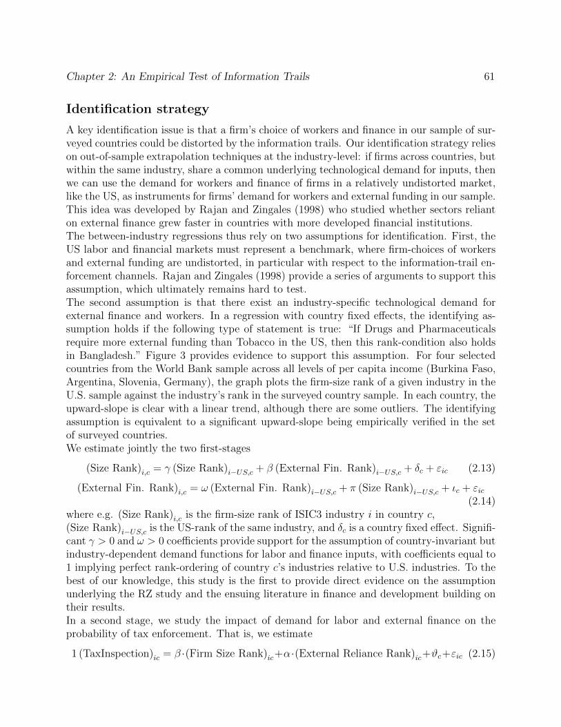
Chapter 2: An Empirical Test of Information Trails 61
Identification strategy
A key identification issue is that a firm’s choice of workers and finance in our sample of sur-veyed countries could be distorted by the information trails. Our identification strategy relieson out-of-sample extrapolation techniques at the industry-level: if firms across countries, butwithin the same industry, share a common underlying technological demand for inputs, thenwe can use the demand for workers and finance of firms in a relatively undistorted market,like the US, as instruments for firms’ demand for workers and external funding in our sample.This idea was developed by Rajan and Zingales (1998) who studied whether sectors relianton external finance grew faster in countries with more developed financial institutions.The between-industry regressions thus rely on two assumptions for identification. First, theUS labor and financial markets must represent a benchmark, where firm-choices of workersand external funding are undistorted, in particular with respect to the information-trail en-forcement channels. Rajan and Zingales (1998) provide a series of arguments to support thisassumption, which ultimately remains hard to test.The second assumption is that there exist an industry-specific technological demand forexternal finance and workers. In a regression with country fixed e↵ects, the identifying as-sumption holds if the following type of statement is true: “If Drugs and Pharmaceuticalsrequire more external funding than Tobacco in the US, then this rank-condition also holdsin Bangladesh.” Figure 3 provides evidence to support this assumption. For four selectedcountries from the World Bank sample across all levels of per capita income (Burkina Faso,Argentina, Slovenia, Germany), the graph plots the firm-size rank of a given industry in theU.S. sample against the industry’s rank in the surveyed country sample. In each country, theupward-slope is clear with a linear trend, although there are some outliers. The identifyingassumption is equivalent to a significant upward-slope being empirically verified in the setof surveyed countries.We estimate jointly the two first-stages
(Size Rank)i,c
= � (Size Rank)i�US,c
+ � (External Fin. Rank)i�US,c
+ �c
+ "ic
(2.13)
(External Fin. Rank)i,c
= ! (External Fin. Rank)i�US,c
+ ⇡ (Size Rank)i�US,c
+ ◆c
+ "ic
(2.14)where e.g. (Size Rank)
i,c
is the firm-size rank of ISIC3 industry i in country c,(Size Rank)
i�US,c
is the US-rank of the same industry, and �c
is a country fixed e↵ect. Signifi-cant � > 0 and ! > 0 coe�cients provide support for the assumption of country-invariant butindustry-dependent demand functions for labor and finance inputs, with coe�cients equal to1 implying perfect rank-ordering of country c’s industries relative to U.S. industries. To thebest of our knowledge, this study is the first to provide direct evidence on the assumptionunderlying the RZ study and the ensuing literature in finance and development building ontheir results.In a second stage, we study the impact of demand for labor and external finance on theprobability of tax enforcement. That is, we estimate
1 (TaxInspection)ic
= � ·(Firm Size Rank)ic
+↵·(External Reliance Rank)ic
+#c
+"ic
(2.15)

Chapter 2: An Empirical Test of Information Trails 62
where the rank of firm size and external reliance may be replaced by their predicted valuesfrom the first stage.Using the rank of firm size as opposed to actual firm size values to predict tax enforcementis motivated by the idea that in the absence of administrative and information constraintswithin a country, tax authorities will e↵ectively target enforcement and auditing towardsindustry-firms in descending order of these industries’ reliance on external finance and laborinputs. Thus actual firm-size and external finance only matter to the extent that theydetermine an industry’s relative location in terms of the country-wide distributions of laborinput and external dependency. A rank-rank regression also provides a more direct test ofthe identification assumption than a regression using actual values.7
2.4 Regression Results
In 4.1 we present the impact of information trails on the probability of tax inspection. In 4.2we go one step further and study the e↵ect of an increase in tax enforcement, predicted bythe information trails, on sales tax compliance. In the final section 4.3 we test the robustnessof the results.
Main results
Table 2 presents the results of information trails on tax inspection. Column 1 presents thelinear regression of tax inspection probability on the surveyed country’s industry-rank interms of workers and finance.8 The results show that while the rank of firm-size positivelypredicts the probability of tax inspection, there is no e↵ect for the external reliance channel.The joint explanatory power of the two trails in determining tax enforcement is strong (F-test equal to 16.07).The non-impact of external reliance may arise if the true relationship between externalfunding and tax inspection is highly non-linear, while our OLS assumes a linear relationship.To get at this, Figure 6 illustrates graphically the regression result of Col.1 of Table 1 usingbinned scatter plots. To construct the left (right) plot, we first take the residuals of the thetax-inspection variable and the firm-size rank (external reliance rank) variable with respect toexternal reliance rank (firm-size rank) and country fixed e↵ects. We then divide the residualfirm-size rank (external reliance rank) into twenty equal-sized groups (vingtiles) and plot themeans of the tax-inspection residual within each bin against the mean value of residual firm-size rank (external reliance rank). The solid line shows the best linear fit estimated on the
7In Appendix A Tables 9-10, we show that using actual industry-average values of size and externalreliance yield very similar results.
8All standard errors are clustered at the country level, to account for country-wide correlation. We useas analytical weights the ratio of country-industry number of firm observations to the total number of firmobservations in the raw Enterprise Survey sample; country-industry averages which reflect a larger underlyingnumber of firms, and thus are likely to be more important and more accurate, receive higher weight in theregression.

Chapter 2: An Empirical Test of Information Trails 63
underlying micro-data using OLS and corresponds to the regression coe�cient for firm-size(external reliance) in Col.1 Table 1.9 The scatter-plot provides no evidence of a non-linearunderlying relationship, and the flat linear OLS provides a good fit. The linear OLS alsoseems to fit well the size-tax inspection scatter plot. This linear relationship substantiatesour choice of modeling the inspection dummy outcome as a linear probability model oversize and external finance inputs.In column 2, we present the reduced form results based on the extrapolation technique wherethe US-industry ranks of firm size and external reliance are used to directly predict cross-industry variation in tax enforcement in the WBES country. The coe�cient on firm sizeis small but highly significant at the 1% level; a one standard deviation increase in the USfirm-size industry-ranking leads to a 2.38 percentage points increase in the probability of taxinspection for that industry in the surveyed country. However, the coe�cient on externalreliance again fails to explain tax inspection.In columns 3 and 4, we study the identifying assumption that industry-di↵erences in US-ranks of firm size and external reliance predict di↵erences in the industry-ranks of the WorldBank countries. Column 3 shows that a one-rank increase in the US-ladder of a given industrypredicts a 0.24 rank increase in the industry-ladder of the WB surveyed country, significantat 1%. The U.S. industry of firm-size rank also seems to positively predict external reliancein the World Bank country industry-rank, again significant at 1%. The US-industry rank inexternal dependency explains positively, albeit with a small coe�cient, firm-size, and evennegatively external reliance; this last result however, is no longer as significant when controlsare added. The joint F-test on the U.S. values in predicting cross-industry ranking in firmsize and external reliance remain large, respectively at 43.34 and 10.13, implying a strongfirst stage.We estimate the joint instrumental variables model (13) � (14) � (15) in column 5. Thefirm-size information trail is again significant at 1% while the external reliance channel isnot significant, despite a first stage F-test in excess of 10. This estimate suggests that aone standard deviation in the surveyed country size-ranking caused by exogenous industry-di↵erences in size and external finance leads to an 8.34 percentage points industry averagetax auditing probability, or a 12% increase at a sample mean tax inspection probability of71%.In Appendix A (Tables 3-4), we report the results for Tables 1-2 when controlling for age,legal status (a dummy for sole proprietorship), exporter status, and reported di�culty inaccessing finance.10 There is a small loss in significance, but the results are largely unchanged.
9The same methodology is used in Chetty et al. (2014)10We do not include the log of sales for several reasons: first, it is likely to be endogenous to our setting;
second, log workers and external finance are arguably amongst the primitives which determine sales volume;third, total sales is not reported for a large set of firms which do disclose worker size and external reliance.

Chapter 2: An Empirical Test of Information Trails 64
Extension to sales tax compliance
As an extension, we study the impact of the information trails on sales tax compliance, bothdirectly and through tax inspection. The industry-average measure of sales tax compliancecomes with the caveats discussed in Section 3; on the other hand, it should be noted thatstudies of corruption and informality ( Svensson 2003, Almeida and Carneiro 2012) have usedthe same survey formulation of the question and interpreted the values as the true measureof own firm behavior.The results from this extension are presented in Table 3.11 In column 1, the simple OLSspecification shows that within country industry-ranked firm-size significantly predicts salestax compliance, while external reliance does not. Again, the non-significance on the externalfinance trail may arise if the true relationship is highly non-linear. Constructed similarly toFigure 6, in Figure 7 we present the graphical results of the regression in Column 1. Theexternal reliance - tax compliance relationship seems to be well approximated by a linearOLS, alleviating concerns of mis-specification in the econometric model.In the reduced-form specification of column 2, US-industry rank di↵erences in firm size arefound to have a significant reduced-form impact on sales tax compliance, while there is nopattern across external reliance ranks. In the double IV estimation, a one standard devi-ation increase in the surveyed country’s size-industry rank, caused by exogenous industry-di↵erences in demand for size and finance, leads to a 4.22 percentage points increase in salestax compliance, significant at 5%.In columns 4-6, we study whether exogenous di↵erences in firm-size and external fundingreliance explain sales tax compliance through tax inspection. Column 4 simply documents apositive correlation between higher tax inspection and sales tax compliance, which is poten-tially a↵ected by endogeneity. In column 5, we therefore use directly the US-industry ranksin firm-size and external reliance; that is, we estimate the IV model in which the secondstage is:
(Sales Tax Compliance)ic
= ✓ · 1 (TaxInspection)ic
+ µc
+ "ic
(2.16)
and the first stage is:
1 (TaxInspection)ic
= � ·(Firm Size Rank)i�US,c
+↵·(External Reliance Rank)i�US,c
+ c
+"ic
(2.17)The estimated impact ✓IV is very large, and significant at 5%: increased tax inspection causedby exogenous industry-di↵erences in labor and finance inputs causes sales tax compliance toincrease by 43.5 percentage points. While the extrapolation technique almost by constructionguarantees orthogonal instruments, it is harder to entirely validate the exclusion restrictionin this IV-setting. There are other plausible mechanisms than tax inspection, through whichfirm-size and external reliance would cause sales tax compliance to increase.Finally in column 6 we estimate the full three stage least squares model. We use the values
11In the firm-level survey data, there are 3330 ISIC3-matched observations which do not report an answerto the sales tax compliance question; this leads to a loss of 88 ISIC3-country observations. Average taxinspection in the two groups are not significantly di↵erent at the 5% level.

Chapter 2: An Empirical Test of Information Trails 65
of external reliance and firm-size in the surveyed country that are predicted by variation inU.S. industry rankings (cols.3-4 of Table 2) to estimate changes in tax inspection, which inturn explains variation in sales tax compliance. Formally, while the third-stage is now (16),the second stage becomes:
1 (TaxInspection)ic
= ! ·(Firm Size Rank)ic
+�·(External Reliance Rank)ic
+⌘c
+"ic
(2.18)
and we add two first stages (13)�(14). The estimated ✓3SLS equals 43.50 and is significant at1%.12 Note that ✓IV and ✓3SLS are very close, suggesting U.S. variation in industry-size andexternal finance explain tax inspection and sales tax compliance mainly through impactingthe surveyed country’s variation in industry size and external reliance.
Robustness checks
Number of days spent with tax inspector as tax enforcement measure
As a continuous measure of tax enforcement, this intensive margin variable of the firm’sreported number of days spent with tax inspectors provides a robustness check to the taxinspection and compliance results. The mean number of days spent with tax inspectors isat 2.23, with a standard deviation of 2.27.The results carry over using this intensive margin variable.13 Full results are reported inAppendix Tables 5-6. The double-IV estimates show that from exogenous changes to tech-nological demand for labour and finance input, increased firm-size leads to an increase of1.18 tax inspection days, significant at 5% (Table A5, Col.5).When instrumented by the U.S. industry-ranks in firm-size and external reliance, one moreday spent with tax inspectors causes sales tax compliance to increase by 2.28 percentagepoints, just below significance at 1%. This ’intensive margin’ e↵ect of increased tax inspec-tion is almost 20 times smaller than the ’extensive margin’ e↵ect estimated using the binarytax inspection dummy (Table 2, Col.5), suggesting that broadening the set of industries in-spected and audited may contribute significantly more to revenue collection than intensifyingenforcement on a smaller set of firms.
12We have not been able to find other papers which estimate a 3SLS with two first stages. Our estimateof ✓3SLS is essentially an IV in the second and third stages ((18) & (16)) and a 2SLS in the first and secondstage; we plug the predicted values from (13) and (14) into (20), then perform an IV using (16) and (18).Parameter estimates are consistent in each stage. If instead we estimated the whole system through a seriesof 2SLS, the coe�cient ✓2x[2SLS] reported in column (7) is equal to 43.51 and significant at 1%.
13In this double instrumental variables model, the second stage is now:
1 (# Days spent with tax inspectors)ic
= � · (Firm Size Rank)ic
+ ↵ · (External Reliance Rank)ic
+ #c
+ "ic
(2.19)and the first stages remain (13)� (14)
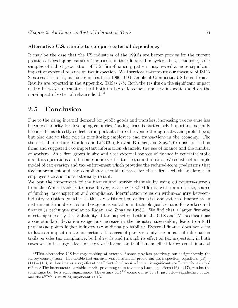
Chapter 2: An Empirical Test of Information Trails 66
Alternative U.S. sample to compute external dependency
It may be the case that the US industries of the 1990’s are better proxies for the currentposition of developing countries’ industries in their finance life-cycles. If so, then using oldersamples of industry-variation of U.S. firm-financing pattern may reveal a more significantimpact of external reliance on tax inspection. We therefore re-compute our measure of ISIC-3 external reliance, but using instead the 1990-1999 sample of Compustat US listed firms.Results are reported in the Appendix, Tables 7-8. Both the results on the significant impactof the firm-size information trail both on tax enforcement and tax inspection and on thenon-impact of external reliance hold.14
2.5 Conclusion
Due to the rising internal demand for public goods and transfers, increasing tax revenue hasbecome a priority for developing countries. Taxing firms is particularly important, not onlybecause firms directly collect an important share of revenue through sales and profit taxes,but also due to their role in monitoring employees and transactions in the economy. Thetheoretical literature (Gordon and Li 2009b, Kleven, Kreiner, and Saez 2016) has focused onfirms and suggested two important information channels: the use of finance and the numberof workers. As a firm grows in size and uses external sources of finance it generates trailsabout its operations and becomes more visible to the tax authorities. We construct a simplemodel of tax evasion and tax enforcement which provides the reduced-form predictions thattax enforcement and tax compliance should increase for these firms which are larger inemployee-size and more externally reliant.We test the importance of the finance and worker channels by using 80 country-surveysfrom the World Bank Enterprise Survey, covering 108,500 firms, with data on size, sourceof funding, tax inspection and compliance. Identification relies on within-country between-industry variation, which uses the U.S. distribution of firm size and external finance as aninstrument for undistorted and exogenous variation in technological demand for workers andfinance (a technique similar to Rajan and Zingales 1998,). We find that a larger firm-sizea↵ects significantly the probability of tax inspection both in the OLS and IV specifications:a one standard deviation exogenous increase in the industry size-ranking leads to a 8.34percentage points higher industry tax auditing probability. External finance does not seemto have an impact on tax inspection. In a second part we study the impact of informationtrails on sales tax compliance, both directly and through its e↵ect on tax inspection: in bothcases we find a large e↵ect for the size information trail, but no e↵ect for external financial
14This alternative U.S-industry ranking of external finance predicts positively but insignificantly thesurvey-country rank. The double instrumental variables model predicting tax inspection, equations (13) �(14) � (15), still estimates a significant coe�cient for firm-size but an insignificant coe�cient for externalreliance.The instrumental variables model predicting sales tax compliance, equations (16)� (17), retains thesame signs but loses some significance. The estimated ✓IV comes out at 39.31, just below significance at 1%;and the ✓3SLS is at 38.74, significant at 1%.

Chapter 2: An Empirical Test of Information Trails 67
dependence. Instrumented by exogenous industry-di↵erences in labor and external finance,an increase in tax inspection leads sales tax compliance to increase by 43.51 percentagepoints.The non-result regarding external funding reliance leaves open the question on why don’t taxadministrations use financial information. One possibility is that the induced misallocationfrom levying the finance information trail is prohibitively large. Another is that politicaleconomy factors prevent tax administrations from systematically accessing this information.A final possibility is that tax authorities of developing countries have not yet made theinvestments in tax capacity to e�ciently manage financial information.

Chapter 2: An Empirical Test of Information Trails 68
Table and Figures
Table 2.1: Tax Inspection Results
Reduced Forms First Stages IV
Tax Inspection Rank WB Worker Rank WB ExtRel Tax InspectionOLS OLS OLS OLS IV(1) (2) (3) (4) (5)
Rank WB Worker .003 .006(.000) *** (.002)***
Rank WB External Reliance .000 .003(.000) (.006)
Rank US Worker .002 .248 .085(.000)*** (.033)*** (.021) ***
Rank US External Reliance .000 .075 -.039(.000) (.035)** (.019)**
F test joint significance 16.07 8.02 43.43 10.13 8.08(.000) (.000) (.000) (.000) (.000)
Observations 2597 2597 2597 2597 2597Clusters 78 78 78 78 78
Standard errors clustered at the country level. All regressions include country fixed e↵ects⇤ p < 0.10, ⇤⇤ p < 0.05, ⇤⇤⇤ p < 0.01
Column (5) is a double IV which uses Cols. (3)-(4) as first stages. See Section 4.2 for more details

Chapter 2: An Empirical Test of Information Trails 69
Table 2.2: Sales Tax Compliance Results
Sales Tax Compliance (Percent)OLS OLS IV OLS IV 3SLS 2*2SLS(1) (2) (3) (4) (5) (6) (7)
Tax Inspection 5.65 43.51 43.51 43.52(2.57)** (17.37)** (17.37)** (14.39)***
Rank WB Worker .202 .317(.034)*** (.145)**
Rank WB Ext Rel -.031 -.032(.027) (.300)
Rank US Worker .076(.026)***
Rank US Ext Rel .025(.028)
F test joint significance 17.28 4.64 4.62(.000) (.012) (.012)
1st Stage (3)-(4)Table1 (2) Table2 (3)-(4)-(5) Table1 (3)-(4)-(5)Table1
Observations 2509 2509 2509 2509 2509 2509 2509Clusters 77 77 77 77 77 77 77
Standard errors clustered at the country level. All regressions include country fixed e↵ects⇤ p < 0.10, ⇤⇤ p < 0.05, ⇤⇤⇤ p < 0.01
Column (6) is a 3SLS where Cols.(3)-(4) Table 1 are first stages, and Col.5 Table 1 is the second stage. Column (7) estimates the 3SLS as a set of 2SLS
See Section 4.2 for more details

Chapter 2: An Empirical Test of Information Trails 70
Figure 2.1: Tax inspection and Sales Tax Compliance Across Firm Size
.5.6
.7.8
.91
Mea
n %
Tax
Insp
ectio
n, S
ales
Tax
Com
plia
nce
1 2 3 4 5 6 7 8 9 10 11 12 13 14 15 16 17 18 19 2020 quantiles of firm−size
Avg Sales Tax Compliance Avg Tax Inspection 95% CI
Figure 2.1 plots averages of sales tax compliance (X-series) and tax inspection (circle-series) across 20quantiles of firm size. The quantiles are constructed based on the pooled sample of country-ISIC3 industryobservations in the World Bank Enterprise database (2,597 observations). Firm size is measured by thereported number of permanent employees in the firm. Tax inspection is the dummy indicator for whetherthe firm had a tax inspection visit over the last year. Sales tax compliance is the share of sales that a firmestimates its competitors report for tax purposes. See section 3.1 for further details.
Figure 2.2: Tax Inspection and Sales Tax Compliance Across External Financial Use
Mass at 0=6 quants
.5.6
.7.8
.91
Mea
n %
Tax
Insp
ectio
n, S
ales
Tax
Com
plia
nce
1 2 3 4 5 6 7 8 9 10 11 12 13 14 15 16 17 18 19 2020 Quantiles of External Finance Reliance
Avg Sales Tax Compliance Avg Tax Inspection 95% CI
Figure 2.2 plots averages of sales tax compliance (X-series) and tax inspection (circle-series) across 20quantiles of share of external financial reliance. The quantiles are constructed based on the pooled sampleof country-ISIC3 industry observations in the World Bank Enterprise database (2,597 observations).External reliance is measured as the percent share of financing which is sourced in retained earnings, familyand friends and informal finance. Firms with zero external reliance represent 34% of the total number offirms. Tax inspection is the dummy indicator for whether the firm had a tax inspection visit over the lastyear. Sales tax compliance is the share of sales that a firm estimates its competitors report for taxpurposes. See section 3.1 for details.
Chapter 2: An Empirical Test of Information Trails 71
Figure 2.3: Distributions of Firm Size Conditional on External Financial Use
0.1
.2.3
.4M
argi
nal d
ensi
ty
0 2 4 6 8 10 12Log permanent workers
0% External Finance EF: 0 < .. < 34% EF >=34%
Figure 2.3 This graph superposes external financial reliance kernel density distributions wheresample-restriction is based on the number of permanent employees at the firm-level. Respectively the blue,red dashed, and green lines depict the external reliance density distribution in the first, second and thirdtercile of the firm-size distribution. External reliance is measured as the percent share of financing which issourced in retained earnings, family and friends and informal finance. Total firm-level sample-size: 108,538.
Figure 2.4: Distributions of External Financial Use Conditional on Firm Size
05
1015
Mar
gina
l den
sity
0 .2 .4 .6 .8 1Share external financial reliance
1st tercile of firm−size dist. 2nd tercile 3rd tercile
Figure 2.4 This graph superposes firm-size kernel density distributions where sample-restriction is based onexternal financial reliance at the firm-level. Respectively the blue, red dashed, and green lines depict thefirm-size density distribution for firms in the first, second, and third terciles of the external reliancedistribution. The first group has zero percent external reliance, the second external reliance strictlypositive but below 34%, and the third group has external reliance greater than 34%. External reliance ismeasured as the percent share of financing which is sourced in retained earnings, family and friends andinformal finance. Total firm-level sample-size: 108,538.

Chapter 2: An Empirical Test of Information Trails 72
Figure 2.5: Firm Size Rank-Rank Relation: U.S. Industries on WB Countries
05
1015
Indu
stry
−ran
k B
urki
na F
aso
0 5 10 15Industry−rank US
Burkina Faso
05
1015
20In
dust
ry−r
ank
Arg
entin
a
0 5 10 15 20Industry−rank US
Argentina0
1020
3040
Indu
stry
−ran
k S
love
nia
0 10 20 30 40Industry−rank US
Slovenia
010
2030
4050
Indu
stry
−ran
k G
erm
any
0 10 20 30 40 50Industry−rank US
Germany
Figure 2.5 plots the rank-rank relation for firm-size in 4 selected WB surveyed countries: Burkina Faso,Argentina; Slovenia; and Germany. Each observation represents the ranking-position of a given ISIC-3industry, in the WB country industry-rank and in the U.S. industry-rank. Blue lines are linear fits. SeeSection 4.2 for details.
Figure 2.6: Impact of Firm Size and External Finance on Tax Inspection
−.2
−.1
5−
.1−
.05
0.0
5.1
.15
.2R
esid
ua
l ta
x in
sp
ectio
n p
rob
ab
ility
−40 −20 0 20 40Residual firm−size rank
−.2
−.1
5−
.1−
.05
0.0
5.1
.15
.2R
esid
ua
l ta
x in
sp
ectio
n p
rob
ab
ility
−40 −20 0 20 40Residual external reliance rank
In Figure 2.6 the right and left panels are binned scatter plots of tax inspection versus respectivelyfirm-size rank and external financial reliance rank. These plots correspond to regression Col.1 of Table 1and use the same sample and variable definitions. To construct the left (right) plot, we first residualize thetax-inspection variable and the firm-size rank (external reliance rank) variable with respect to externalreliance rank (firm-size rank) and country fixed e↵ects. We then divide the residual firm-size rank (externalreliance rank) into twenty equal-sized groups (vingtiles) and plot the means of the tax-inspection residualwithin each bin against the mean value of residual firm-size rank (external reliance rank). The solid lineshows the best linear fit estimated on the underlying microdata using OLS and corresponds to theregression coe�cient for firm-size (external reliance) in Col.1 Table 1.

Chapter 2: An Empirical Test of Information Trails 73
Figure 2.7: Impact of Firm Size and External Finance on Sales Tax Compliance
−1
0−
50
51
0R
esid
ua
l sa
les t
ax c
om
plia
nce
−40 −20 0 20 40Residual firm−size rank
−1
0−
50
51
0R
esid
ua
l sa
les t
ax c
om
plia
nce
−40 −20 0 20 40Residual external reliance rank
In Figure 2.7 the right and left panels are binned scatter plots of sales tax compliance versus respectivelyfirm-size rank and external financial reliance rank. These plots correspond to regression Col.1 of Table 2and use the same sample and variable definitions. To construct the left (right) plot, we first residualize thesales tax compliance variable and the firm-size rank (external reliance rank) variable with respect toexternal reliance rank (firm-size rank) and country fixed e↵ects. We then divide the residual firm-size rank(external reliance rank) into twenty equal-sized groups (vingtiles) and plot the means of the sales taxcomplianxe residual within each bin against the mean value of residual firm-size rank (external reliancerank). The solid line shows the best linear fit estimated on the underlying microdate using OLS, andcorresponds to the regression coe�cient for firm-size (external reliance) in Col.1 Table 2.

Chapter 2: An Empirical Test of Information Trails 74
2.6 Appendix A: Additional Results
• Table 3: Tax inspection results with a set of country-industry specific controls: age,legal status, exporter status, self-reported financial constraints.
• Table 4: Sales tax compliance results with a set of country-industry specific controls:age, legal status, exporter status, self-reported financial constraints.
• Table 5: Tax inspection results using self-reported number of days spent with taxinspector as outcome variable (instead of binary tax inspection variable used in maintext).
• Table 6: Sales tax compliance results using self-reported number of days spent as taxinspection variable.
• Table 7: Tax inspection results using Compustat 1990-99 sample to compute USindustry-averages of financial external reliance.
• Table 8: Sales tax compliance results using Compustat 1990-99 sample to compute USindustry-averages of financial external reliance.
• Table 9: Tax inspection results using actual firm size and share of external reliance.
• Table 10: Sales tax compliance results using actual firm size and share of reliance.

Chapter 2: An Empirical Test of Information Trails 75
Table 2.3: Tax Inspection Results with Controls
Reduced Forms First Stages Double IV
Tax Inspection Rank WB Worker Rank WB ExtRel Tax InspectionOLS OLS OLS OLS IV(1) (2) (3) (4) (5)
Rank WB Worker .003 .007(.000)*** (.004)*
Rank WB External Reliance .000 .001(.000) (.007)
Rank US Worker .001 .166 .089(.000)*** (.028)*** (.022)***
Rank US External Reliance .000 .049 -.037(.000) (.028)* (.020)*
F test joint significance 10.34 4.35 26.54 9.10 4.01(.000) (.016) (.000) (.000) (.022)
Controls included Age, legal status, exporter status, reported financial constraints
Observations 2532 2532 2532 2532 2532Clusters 77 77 77 77 77
Standard errors clustered at the country level. All regressions include country fixed e↵ects⇤ p < 0.10, ⇤⇤ p < 0.05, ⇤⇤⇤ p < 0.01
Table 2.4: Sales Tax Compliance Eesults with Controls
Sales Tax Compliance (Percent)OLS OLS IV OLS IV 3SLS 2*2SLS(1) (2) (3) (4) (5) (6) (7)
Tax Inspection 4.88 42.41 42.41 42.0(2.53)* (24.67)* (24.67)* (19.84)**
Rank WB Worker .161 .291(.042)*** (.221)
Rank WB Ext Rel -.019 .072(.028) (.369)
Rank US Worker .056(.025)**
Rank US Ext Rel .010(.026)
F test joint significance 7.52 2.42 2.61(.001) (.095) (.080)
1st Stage (3)-(4)Table3 (2)Table4 (3)-(4)Table3 (3)-(4)-(5)Table3
Controls included Age, legal status, exporter status, reported financial constraintsObservations 2449 2449 2449 2449 2449 2449 2449Clusters 76 76 76 76 76 76 76
Standard errors clustered at the country level. All regressions include country fixed e↵ects⇤ p < 0.10, ⇤⇤ p < 0.05, ⇤⇤⇤ p < 0.01

Chapter 2: An Empirical Test of Information Trails 76
Table 2.5: Tax Inspection Results when Tax Inspection is Number of Days
Reduced Forms First Stages Double IV
Tax Inspection nr. Days Rank WB Worker Rank WB ExtRel Tax Inspection nr. daysOLS OLS OLS OLS IV(1) (2) (3) (4) (5)
Rank WB Worker .047 .089(.009)*** (.037)**
Rank WB External Reliance .010 .135(.009) (.127)
Rank US Worker .033 .248 .085(.007)*** (.033)*** (.021)***
Rank US External Reliance .001 .075 -.039(.005) (.035)** (.019)**
F test joint significance 15.05 10.02 43.34 10.13 11.27(.000) (.016) (.000) (.000) (.022)
Observations 2597 2597 2597 2597 2597Clusters 78 78 78 78 78
Standard errors clustered at the country level. All regressions include country fixed e↵ects⇤ p < 0.10, ⇤⇤ p < 0.05, ⇤⇤⇤ p < 0.01
Table 2.6: Sales Tax Compliance when Tax Inspection is Number of Days
Sales Tax Compliance (Percent)OLS OLS IV OLS IV 3SLS 2*2SLS(1) (2) (3) (4) (5) (6) (7)
Tax Inspection Nr. Days .093 2.28 2.28 2.39(.090) (.922)** (.922)** (.795)***
Rank WB Worker .161 .291(.042)*** (.221)
Rank WB Ext Rel -.019 .072(.028) (.369)
Rank US Worker .056(.025)**
Rank US Ext Rel .010(.026)
F test joint significance 7.52 2.42 2.61(.001) (.095) (.080)
1st Stage (3)-(4)Table5 (2)Table6 (3)-(4)Table5 (3)-(4)-(5)Table5hline
Observations 2509 2509 2509 2509 2509 2509 2509Clusters 77 77 77 77 77 77 77
Standard errors clustered at the country level. All regressions include country fixed e↵ects⇤ p < 0.10, ⇤⇤ p < 0.05, ⇤⇤⇤ p < 0.01

Chapter 2: An Empirical Test of Information Trails 77
Table 2.7: Tax Inspection Results Using Alternative Sample for US External Finance
Reduced Forms First Stages Double IV
Tax Inspection Rank WB Worker Rank WB ExtRel Tax InspectionOLS OLS OLS OLS IV(1) (2) (3) (4) (5)
Rank WB Worker .003 .005(.000) *** (.002)*
Rank WB External Reliance .000 .005(.000) (.010)
Rank US Worker .001 .274 .078(.000)*** (.031)*** (.022) ***
Rank US Ext Rel 1990-99 .000 .132 -.010(.000) (.031)*** (.031)
F test joint significance 16.07 11.60 44.98 7.45 9.47(.000) (.000) (.000) (.001) (.000)
Observations 2597 2597 2597 2597 2597Clusters 78 78 78 78 78
Standard errors clustered at the country level. All regressions include country fixed e↵ects⇤ p < 0.10, ⇤⇤ p < 0.05, ⇤⇤⇤ p < 0.01
Table 2.8: Sales Tax Compliance Results Using Alternative Sample for US External Finance
Sales Tax Compliance (Percent)OLS OLS IV OLS IV 3SLS 2*2SLS(1) (2) (3) (4) (5) (6) (7)
Tax Inspection 5.65 39.31 39.31 38.749(2.57)** (14.99)** (14.99)** (12.73)***
Rank WB Worker .202 .119(.034)*** (.177)
Rank WB Ext Rel -.031 .603(.027) (.694)
Rank US Worker .081(.026)***
Rank US Ext Rel 1990-99 .011(.022)
F test joint significance 17.28 4.71 5.31(.000) (.011) (.006)
1st Stage (3)-(4)Table7 (2)Table8 (3)-(4)Table7 (3)-(4)-(5)Table7
Observations 2509 2509 2509 2509 2509 2509 2509Clusters 77 77 77 77 77 77 77
Standard errors clustered at the country level. All regressions include country fixed e↵ects⇤ p < 0.10, ⇤⇤ p < 0.05, ⇤⇤⇤ p < 0.01

Chapter 2: An Empirical Test of Information Trails 78
Table 2.9: Tax Inspection Results with Alternative Non-Rank Measures of Firm Size andExternal Finance
Reduced Forms First Stages Double IV
Tax Inspection Lg Firm Size WB Share Ext Rel WB Tax InspectionOLS OLS OLS OLS IV(1) (2) (3) (4) (5)
Lg Firm Size WB .040 .172(.006) *** (.112)
Share Ext Rel WB .018 -.781(.017) (1.04)
Lg Firm Size US .025 .303 .034(.007)*** (.039)*** (.007) ***
Share Ext Rel US .006 .021 -.003(.003) (.015) (.005)
F test joint significance 19.23 8.82 37.90 9.75 3.93(.000) (.000) (.000) (.000) (.023)
Observations 2597 2597 2597 2597 2597Clusters 78 78 78 78 78
Standard errors clustered at the country level. All regressions include country fixed e↵ects⇤ p < 0.10, ⇤⇤ p < 0.05, ⇤⇤⇤ p < 0.01
Table 2.10: Sales Tax Compliance Results with Alternative Non-Rank Measures of Firm Sizeand External Finance
Sales Tax Compliance (Percent)OLS OLS IV OLS IV 3SLS 2*2SLS(1) (2) (3) (4) (5) (6) (7)
Tax Inspection 5.65 49.37 49.37 50.85(2.57)** (16.35)*** (16.35)*** (16.41)***
Lg Firm Size WB 2.415 .527(.371)*** (.423)
Share Ext Rel WB -.367 -93.43(.902) (88.38)
Lg Firm Size US .753(.483)***
Share Ext Rel US .677(.207)***
F test joint significance 21.97 6.82 1.04(.000) (.001) (.359)
1st Stage (3)-(4)Table9 (2)Table10 (3)-(4)Table9 (3)-(4)-(5)Table9
Observations 2509 2509 2509 2509 2509 2509 2509Clusters 77 77 77 77 77 77 77
Standard errors clustered at the country level. All regressions include country fixed e↵ects⇤ p < 0.10, ⇤⇤ p < 0.05, ⇤⇤⇤ p < 0.01

Chapter 2: An Empirical Test of Information Trails 79
2.7 Appendix B: Data Sources
Throughout the analysis the unit of observation is a country-industry, where industries areclassified using the ISIC 3 digit methodology, produced by the U.N. Statistics Division. TheISIC3 methodology classifies distinct and refined groups; per example, ’Manufacture of dairyproducts’ is classified as ISIC152, while ’Manufacture of grain mill products, starches andstarch products, and prepared animal feed’ is classified as ISIC153.The World Bank Enterprise Survey is the primary data source: this is a firm level surveycollected by the World bank between 2002 and 2010 in more than a hundred countries. Toour knowledge this is the only standardized firm data set spanning countries across the de-velopment spectrum. Since the survey was clearly administered by a third party not relatedto the government or the statistical o�ce it could ask unique questions on tax behavior andcorruption.We also rely on two other data sources to construct our instrumental variables: the Compu-stat database of firms listed in the stock exchange in the US and the U.S. Bureau of LabourStatistics Quarterly Census of Employment and Wages. We mapped the U.S. industry cod-ing, NAICS, into the ISIC classification using the appropriate U.N. tables and merged U.S.industry-averages with the industry averages from the Enterprise Survey based on commonISIC3 codes. The final sample is 2597 country-ISIC3 observations from 77 countries.
Tax inspection and tax compliance
We use the firm’s reported answer to the question: “Total days spent with o�cials from: taxinspectorate.” In particular we construct a tax inspection dummy equal to one if the firmhas been visited for at least one day by tax auditors. The industry-average tax inspectionprobability is .71, with a standard deviation of .35. This is the main measure of tax enforce-ment that we use throughout the main text.We also use the question on sales tax evasion: “Recognizing the di�culties many enterprisesface in fully complying with taxes and regulations, what percentage of total sales would youestimate the typical establishment in your area of activity reports for tax purposes?” Thereare obvious di�culties in assuming that the firm’s answer to this question reflects its ownindustry tax evasion and even harder that it is the firm’s own evasion level.
External reliance
To construct a measure of external reliance, we strictly follow the methodology presented inRajan and Zingales 1998 (RZ hereafter). The measure of external dependence proxies forthe amount of investment that cannot be financed through internal sources, i.e. the retainedearnings generated by the business. For the U.S. values of this measure, we use Compustatover the years 2000-2012, and compute external reliance as the ratio of capital expendituresminus cash flow from operations divided by capital expenditures. For each firm, we sumthe numerator and denominator over time before dividing, with the intention of smoothing

Chapter 2: An Empirical Test of Information Trails 80
temporal fluctuations. As in RZ we use the industry median, to reduce the impact of largerfirms. For the decades after 1990, the reporting in Compustat changes from the original RZsample. We follow the instructions in RZ and the conventions in the finance literature toconstruct the measure of external reliance.In the World Bank sample, firm’s balance sheets give information on the shares of financ-ing from di↵erent sources of earnings. The measure of external reliance is defined as theratio of external sources’ share over the sum of external and internal shares: share ext
i
=externali
externali+internaliInternal finance is the sum of retained earnings, friends and family and infor-
mal finance. External finance is defined as banking finance which incudes loans, overdraftsand credit card finance. An important advantage of the Enterprise Surveys is the possibilityto construct the same measure of external reliance in both the World Bank and the Com-pustat sample. In the Enterprise Survey, the industry-average external reliance is .38, witha standard deviation of .47. Table 1 provides some summary statistics for sources of firm-financing, distinguishing between finance-sources for working capital and for new investment.In both cases, retained earnings is the dominant method of financing, with respectively 63.9and 63.8 percent of working capital and new investment financed through the internal cashflow of the firm. Bank finance comes second for both capital and investment, at respectively15.4 and 19.6 percent.For some sources of financing it is ambiguous whether they generate any tax-relevant infor-mation trail (such as trade credit and leasing arrangements). In all results presented, theyare excluded when constructing our measure of external reliance.
Table 2.11: Summary of Financing Sources
Working Capital New Investmentmean sd mean sd
Retained earnings 63.9 38.0 63.8 42.2Bank finance 15.4 27.5 19.6 34.3Trade credit 11.8 22.5 4.3 16.5Friends 3.7 13.8 3.5 15.1Non bank finance 1.6 9.3 1.9 11.5Other 3.3 14.2 5.6 19.8N 69985 43869
Firm size
We choose as number of workers the Enterprise Survey firm’s reported average number ofpermanent workers. Workers which are permanent employees are more likely to have accessto the internal books of the firm and thus are more able than temporary employees to “blow
Chapter 2: An Empirical Test of Information Trails 81
the whistle” and report tax under-reporting. The sample-wide distribution of firms has heavynegative skew, with a long right tail: while the median is at 17 workers, the mean of 105is largely influenced by a few very large firms. Given the shape of the marginal density, wealways use the natural log of firm size in the regressions. We retrieve data in the U.S. fromthe 2002 version of the Census of Employment and Wages to U.S. ISIC3-specific averagefirm-size.

82
Chapter 3
Banking on Trust: How Debit CardsEnable the Poor to Save
with Paul Gertler, Sean Higgins & Enrique Seira
3.1 Introduction
Trust is an essential element of economic transactions and an important driver of economicdevelopment (Banfield 1958; Knack and Keefer 1997; Porta et al. 1997; Narayan and Pritch-ett 1999; Algan and Cahuc 2010). Trust is the “subjective probability with which an agentassesses that another . . . will perform a particular action (Gambetta 1988, p. 217). It isparticularly important in financial transactions where people pay money in exchange forpromises, and essential where the legal institutions that enforce contracts are weak (McMil-lan and Woodru↵ 1999; Karlan et al. 2009). Given the nature of financial decisions, it isnot surprising that trust has been shown to be key to stock market participation (Guiso,Sapienza, and Zingales 2008), use of checks instead of cash (Guiso, Sapienza, and Zingales2004), and decisions to not withdraw deposits from financial institutions in times of financialcrisis (Iyer and Puri 2012; Sapienza and Zingales 2012).
Trust in financial institutions is low, as evidenced by the fact that majorities in 40percent of countries included in the World Values Survey report lack of confidence in banks(Figure 3.1). Trust is especially low among the poor. In Mexico, for example, 71% of thosewith less than primary school report low trust in banks, compared to 55% of those whocompleted primary school and 46% of those who completed university (Figure 3.2). Alongwith fees and minimum balance requirements, trust is frequently listed as a primary reasonfor not saving in formal bank accounts (e.g., Dupas et al. 2016). At the country level, lowtrust in financial institutions is strongly correlated with the proportion of the populationwithout bank accounts (Figure 3.3). Despite its importance, trust as a potential barrier to

Chapter 3: Banking on Trust 83
the poor saving in financial institutions has not been extensively studied (Karlan, Ratan,and Zinman 2014).1
Lack of trust in financial institutions may not be unfounded. Cohn, Fehr, and Marchal(2014) provide evidence that the banking industry fosters a culture of dishonesty relative toother industries. In Mexico in particular, bankers have been found to loot money by directinga large portion of bank lending to “related parties,” i.e. shareholders of the bank and theirfirms (La Porta, Silanes, and Zamarripa 2003). Mexican newspapers report many instancesof outright bank fraud where depositors have lost their savings. For example, an extensivelycovered scandal involved Ficrea whose majority shareholder reportedly stole USD 200 millionfrom savers (CNBV 2014).2 It is also telling that articles with financial advice in Mexicannewspapers have titles like “How to Save for Your Graduation and Avoid Frauds” and“Retirement Savings Accounts, with Minimal Risk of Fraud.” When contract enforcementis poor and fraud is rampant, trust becomes even more important (Guiso, Sapienza, andZingales 2004; Karlan et al. 2009) and people are understandably even more reluctant to useuntrustworthy financial institutions (Bohnet, Herrmann, and Zeckhauser 2010).
While trust is important, it is not an innate characteristic but rather can be influencedby experience and information (Hirschman 1984; Williamson 1993; Attanasio, Pellerano,and Reyes 2009). Debit cards (and mobile money) provide a low cost technology to monitoraccount balances and thereby build trust that a bank will neither explicitly steal deposits norcharge unexpectedly large hidden fees. Previous studies on debit cards and mobile moneyhave focused on the e↵ect of the lower transaction costs facilitated by these technologies tomake purchases (Zinman 2009), access savings and remittances (Suri, Jack, and Stoker 2012;Schaner forthcoming), and transfer money (Jack, Ray, and Suri 2013; Jack and Suri 2014),but not their capacity to monitor and build trust in financial institutions. We hypothesizethat new debit card clients first use the cards to check balances and thereby establish trust,after which they take advantage of the cards lower transaction costs to use the servicesof formal financial institutions. In this sense, we argue that building trust in a financialinstitution is a necessary condition for the use of formal financial services; i.e., financialinclusion requires trust. Indeed, a lack of trust could explain why a number of randomizedfield experiments have found that even when take-up of accessible and a↵ordable formalsavings products is high, use is low in that most opened accounts have few transactions afterthe first 6 to 12 months (Ashraf, Karlan, and Yin 2006; Dupas and Robinson 2013a; Karlanand Zinman 2014; Schaner 2015).
We examine this hypothesis in the context of a natural experiment in which debit cardswere rolled out geographically over time to beneficiaries of the Mexican conditional cashtransfer program Oportunidades. The beneficiaries had been receiving their transfers into
1Increased trust is proposed—but not explored further—as one channel through which no-fee savingsaccounts led to saving in Prina (2015).
2This type of fraud is not uncommon: we scraped the online news archives of all electronic newspapersand news websites we could find in Mexico (129 total) using several keywords, then filtered the results byhand to keep only relevant stories. We found 1338 news stories associated with savings fraud in 2014 and2015 alone.

Chapter 3: Banking on Trust 84
savings accounts for five years on average before debit cards were attached to their accounts,but typically did not use the accounts to save as they immediately withdraw most if notall of the transfer.3 The phased geographic rollout provides plausibility exogenous variationin assignment of debit cards to beneficiaries in a di↵erence in di↵erence context. For theanalysis, we use high frequency administrative data on bank transactions for over 340,000beneficiary accounts in 370 bank branches over 4 years as well as several household surveysof a sample of the same beneficiaries.
Using the high frequency administrative data, we find that beneficiaries initially useddebit cards to check account balances without any increase in savings, but over time thefrequency of account balance checks fell and savings rates rose. We estimate that after oneyear, the share of total income saved each payment period increased by 5 percentage pointsand that after nearly two years those with cards saved 8 percentage points more per period.
The delayed initiation of savings suggests some kind of learning. We explore three kindsof learning that may be occurring: (i) learning to trust the bank, (ii) learning to use thedebit cards and ATMs, and (iii) learning that the program will not drop beneficiaries whoaccumulate savings. Using household survey data, we find support for the learning to trusthypothesis but not for the other two types of learning. Specifically, we find that 27 percentof beneficiaries who have had the debit card for less than 6 months report that they do nottrust the bank, compared to just 17 percent of those who have had the card for more than 6months. We find very few beneficiaries who report not knowing how to use the technologyor fear the program will drop them if they accumulate savings, and no change over timecomparing those that have had the debit card less than and more than 6 months. We alsofind that those who have had the card more than 6 months report checking their balancessignificantly less frequently than those who have had the card less than 6 months, consistentwith our finding from administrative data that when beneficiaries first get the debit card,they check their balances often, but the frequency of checking falls over time.
We then test whether the increase in the bank account balances is an increase in totalsavings or a substitution from other forms of saving, both formal and informal. Using panelhousehold survey data, we find that after one year the treatment group increases total savingsby about 5 percent of income relative to the control group, which is close in magnitude tothe e↵ect we see in the administrative account data. We find no di↵erential change inincome or assets in the treatment group compared to the control. These results suggest thatthe increase in saving is not driven by higher income but by (voluntarily) lowering currentconsumption and that that the increase in bank savings does not crowd out other forms ofsaving (consistent with Ashraf, Karlan, and Yin 2015; Dupas and Robinson 2013a; Kast,Meier, and Pomeranz 2012).
Finally, a portion of the increase in savings in achieved through a decrease in the con-sumption of alcohol, tobacco, and sugar—the most frequently mentioned temptation goods
3This is consistent with findings from other countries such as Brazil, Colombia, and South Africa, inwhich cash transfers are paid through bank accounts, but recipients generally withdraw the entire transferamount each pay period and do not save in the account (Bold, Porteous, and Rotman 2012).

Chapter 3: Banking on Trust 85
in Banerjee and Mullainathan (2010). Indeed, this is the only consumption category witha statistically significant decrease after receiving the card. Although the poor do save viacash at home (Collins et al. 2009), saving informally is harder as the money is hot andsusceptible to temptation spending, either by the beneficiary herself or by her husband ifshe lacks control over his access to her savings (Ashraf 2009). Indeed, we also find thatamong beneficiaries living with a spouse or partner, those with lower baseline bargainingpower relative to their spouse have a higher increase in savings after receiving the debitcard. Our results suggest that saving in formal financial institutions may help solve someof the intra-household bargaining and self-control problems associated with trying to saveinformally.
These results are important for public policy as building savings in formal financialinstitutions has positive welfare e↵ects for the poor and nearly half of the world’s adultsdo not use financial institutions (Demirg-Kunt et al. 2015). The poor have used savingsproducts to decrease income volatility (Chamon, Liu, and Prasad 2013), accumulate moneyfor microenterprise investments (Dupas and Robinson 2013a), invest in preventative healthproducts and pay for unexpected health emergencies (Dupas and Robinson 2013b), andinvest in childrens education (Prina 2015). Various randomized experiments have foundthat providing a↵ordable and accessible savings accounts to the poor increases their futureagricultural/business output and household consumption (Brune et al. 2016; Dupas andRobinson 2013a), decreases debt (Kast, Meier, and Pomeranz 2012; Atkinson et al. 2013),and improves their ability to cope with shocks (Prina 2015). For these reasons, Mullainathanand Shafir (2009) conclude that access to formal savings services may provide an importantpathway out of poverty.
Given our results, government cash transfer programs could be a promising channelto increase financial inclusion and enable the poor to save, not only because of the sheernumber of the poor that are served by cash transfers, but also because many governmentsare already embarking on digitizing their cash transfer payments through banks and mobilemoney. Furthermore, the technologies of debit cards and ATMs or point of sale (POS)terminals—which can be used to check balances and access savings—are simple, prevalent,and potentially scalable to millions of government cash transfer recipients worldwide.
3.2 Institutional Context
We examine the the rollout of debit cards to urban beneficiaries of Mexicos conditionalcash transfer program Oportunidades whose benefits were already being deposited directlyinto savings accounts without debit cards. Oportunidades is one of the largest and mostwell-known conditional cash transfer programs worldwide with a history of rigorous impactevaluation (e.g., Gertler 2004; Parker and Teruel 2005). The program provides bimonthlycash transfers to poor families in Mexico, seeking to alleviate poverty in the short term andbreak the intergenerational poverty cycle in the long term by requiring families to invest inthe human capital of childen by sending their children to school and having health check-ups.

Chapter 3: Banking on Trust 86
It began in rural Mexico in 1997 under the name Progresa, and later expanded to urbanareas starting in 2002. Today, nearly one-fourth of Mexican households receive benefits fromOportunidades (Levy and Schady 2013).
Oportunidades opened savings accounts in banks for a portion of beneficiaries in ur-ban localities and began depositing the transfers directly into those accounts. The originalmotives for paying through bank accounts were to (i) decrease corruption as automatic pay-ments through banks lowers both the ability of corrupt local o�cials to skim o↵ benefits andof local politicians to associate themselves with the program through face-to-face contactwith recipients when they receive their transfers, (ii) decrease long wait times for recipientswho previously had to show up to a “payment table” on a particular day to receive theirbenefits, (iii) decrease robberies and assaults of program o�cers and recipients transportingcash on known days, and (iv) increase the financial inclusion of poor households. By theend of 2004, over one million families received their benefits directly deposited into savingsaccounts in Bansefi, a government bank created to increase savings and financial inclusionof underserved populations (Figure 3.4).4
The Bansefi savings accounts have no minimum balance requirement or monthly fees andpay essentially no interest.5 Before the introduction of debit cards, beneficiaries could onlyaccess their money at Bansefi bank branches. Because there are only about 500 Bansefibranches nationwide, many beneficiaries live far from their nearest branch, meaning thataccessing their accounts involved large transaction costs for many beneficiaries. Overall, thesavings accounts were barely used prior to the introduction of debit cards. In 2008, theyear before the rollout of debit cards, the average number of deposits per bimester6 was 1.05including the deposit from Oportunidades, the average number of withdrawals was 1.02, and98.9 percent of the transfer was taken during the first withdrawal following payment.
In 2009, the government announced that they would issue Visa debit cards to beneficiariesthat were receiving their benefits directly deposited into Bansefi savings accounts. The cardsenabled account holders to withdraw cash from, make deposits into, and check balances oftheir account at any banks ATM as well as make electronic payments at any store acceptingVisa. The cards included two free ATM withdrawals every bimester at any banks ATM,after which ATM withdrawal fees averaged 13 pesos (about $1 using 2009 exchange rates)but varied by bank.
Opportunities used direct deposit into savings accounts for its beneficiaries in 275 out ofMexicos 550 urban localities. Of these, debit cards were rolled out to approximately 100,000beneficiaries in 143 localities in 2009 (wave 1) and to an additional 75,000 beneficiaries in88 localities in late 2010 (wave 2). Another 170,000 beneficiaries in the remaining localities
4Originally Oportunidades partnered with two banks: Bansefi, a government bank, and Bancomer, acommercial bank. However, working with a commercial bank proved to be di�cult, and Oportunidadesphased out the Bancomer accounts and transferred them to Bansefi by mid-2006.
5Nominal Interest rates were between 0.09 and 0.16 percent per year compared to an inflation of around5 percent per year during our sample period.
6The program is paid in two-month intervals, which we refer to throughout the paper as bimesters. (TheSpanish word bimestre is more common than its English cognate, and is used by Bansefi and Oportunidades.)

Chapter 3: Banking on Trust 87
were scheduled to receive cards between November 2011 and February 2012 (control group)after the end date of our data period. The map in Figure 3.5 shows that the treatment andcontrol waves had substantial geographical breadth and that some treatment and controllocalities were physically close.
The sequence with which localities switched was determined as a function of the pro-portion of households in the locality that were eligible for the program but were not yetreceiving benefits. This is because the introduction of debit cards to existing recipients wascoupled with an e↵ort to incorporate more beneficiaries. Table 3.1 compares the meansof locality-level variables and account-level variables from the control, wave 1, and wave 2localities using data from the population census from 2005, poverty estimates from Oportu-nidades from 2005, Bansefi branch locations from 2008, and the administrative account dataon average balances and transactions from Bansefi in 2008. Column 6 shows the p-valueof an F-test of equality of means. Because the rollout was not random, it is not surprisingthat there are some di↵erences across treatment and control localities: treatment localitiesare slightly larger and beneficiaries in these localities receive higher transfer amounts. Thepercent of the transfer withdrawn also di↵ers (it is lower in wave 1 than the control andinsignificantly di↵erent but with a higher point estimate in wave 2), but is high in all cases(ranging from 97.5 percent to 99.6 percent of the transfer), indicating very low savings inthe account prior to receiving the card. In Sections 3.4 and 3.9, we will test and show thattrends of saving, income and consumption were parallel across waves.
3.3 Data
We use a rich combination of administrative and survey data sources. To examine the e↵ectof rollout of the debit cards on savings we use administrative data from Bansefi at the accountlevel for 342,709 accounts at 380 Bansefi branches for a four-year period, from November2007 to October 2011. These data include the bimonthly transfer amount the timing andamount of transactions made in the account, bimonthly average savings balances, the datethe savings account was opened, and the month the card was awarded to the account holder.The average account had been opened 5.3 years before getting the card.
To test whether the delayed savings e↵ect and increasing propensity to save over timecan be explained by learning to use the technology, learning the program rules, or buildingtrust in the bank, we use the Survey of Urban Households Sociodemographic Characteristics(ENCASDU), conducted by Oportunidades at the end of 2010. We also use the PaymentMethod Survey, a household survey conducted by Oportunidades in 2012 aimed at elicitingsatisfaction with and use of the debit cards.
To explore whether the increased savings in the Bansefi accounts is an increase in overallsavings or a substitution from other forms of saving, we use the Survey of Urban HouseholdCharacteristics (ENCELURB), a panel survey with three pre-treatment waves in 2002, 2003,and 2004, and one post-treatment wave conducted from November 2009 to early 2010. Thissurvey has comprehensive modules on consumption, income, and assets. We merge these data

Chapter 3: Banking on Trust 88
with administrative data from Oportunidades on the transfer histories for this sample—which we use to add transfer income into total income and to identify which householdsare Oportunidades recipients, given the common misreporting of transfer receipt in surveys(Meyer, Mok, and Sullivan 2015)—and on the dates that debit cards were distributed ineach locality.
Because the final pre-treatment wave of ENCELURB in 2004 is five years prior to wave1 of the debit card rollout, we supplement our parallel trends test in ENCELURB with datafor the intervening period (2004-2008) from the National Household Income and Expen-diture Survey (ENIGH), a repeated cross-section; we merge the publicly available ENIGHwith restricted-access locality identifiers provided by the National Institute of Statistics andGeography (INEGI) to determine which surveyed households were in treatment and controllocalities, and restrict the analysis to the poorest 20 percent of surveyed households to proxyfor Oportunidades recipients.
Figure 3.4a shows the timing of the administrative Bansefi account balance and trans-action data, while Figure 3.4b shows the timing of the household survey data (merged withadditional administrative data) we use, both relative to the rollout of debit cards.
3.4 E↵ect of Debit Cards on Stock of Savings
Figure 3.6 presents average balances over time; even the raw data are very telling. Panel (a)compares the first wave of debit card recipients to the control group, with a dashed verticalline indicating the time when wave 1 localities received debit cards, while Panel (b) comparesthe second wave to the control, with a dashed vertical line indicating the time when wave 2localities received debit cards. Strikingly, average balances increase sharply for the first waveafter receiving the card, but the e↵ect is not immediate: it begins about four bimesters afterreceiving the card and the larger increase happens after a year with the card. By October of2011, wave 1 has average balances of around 2000 pesos, over three times that of the controlgroup. Average balances also increase over time with the card in wave 2, although we haveinformation for less bimesters after wave 2’s later switch to debit cards.
Although our data on average balances is by bimester, some payments get shifted tothe end of the prior bimester, so we group adjacent bimesters into four-month periods forthe remainder of the analysis. Because we have four years of data, this leaves us with 12four-month periods. To compare the stock of savings in the treatment and control groupswhile controlling for individual observables and unobservables, as well as any common timeshocks, we use a period-by-period di↵erence-in-di↵erences (DID) strategy and estimate:
Balanceit
= �i
+ �t
+12X
k=1
�k
Tj(i) ⇥ I(t = k) + "
it
(3.1)
where Balanceit
is the average balance in account i over period t (specifically, end of daybalances were averaged over the number of days in the bimester by Bansefi, and we average

Chapter 3: Banking on Trust 89
the average balances over the two adjacent bimesters that make up the four-month period).Following other papers measuring savings (chetty14; e.g., Kast, Meier, and Pomeranz 2012;Mel, McIntosh, and Woodru↵ 2013; Karlan and Zinman 2014; Akbas et al. 2015; Dupaset al. 2016), we winsorize average balances to avoid results driven by outliers; our mainresults winsorize at the 95th percentile, and the results are robust to other cut-o↵s.7 The �
i
are account-level fixed e↵ects which control for observable and unobservable time-invariantcharacteristics of the beneficiaries, �
t
are time-period dummies that control for general macrotrends such as bimester-specific shocks that a↵ect both treatment and control groups, T
j(i) =1 if locality j in which account holder i lives is a treatment (i.e., wave 1 or 2) locality, andI(t = k) are time period dummies. Thus, the T
j(i) ⇥ I(t = k) terms pick up the di↵erence inbalances between treatment and control localities in each period. We estimate cluster-robuststandard errors, "
it
, clustering by Bansefi branch. Since one time period dummy must beomitted from (3.1), we follow the standard procedure of omitting the four-month periodimmediately preceding the change to cards. We estimate (3.1) separately for wave 1 andwave 2.
The coe�cients of interests are the �k
s, which measure the average di↵erence in balancesbetween the control and treatment group in bimester k. The raw data clearly suggest thatpre-treatment trends of savings were parallel across control and treatment groups beforegetting the card; we test this statistically by testing �1 = · · · = �
`�1 = 0 where ` is theperiod of switch. (In wave 1, ` is the period November 2009-February 2010, and in wave2 it is the period November 2010-February 2011.) Figure 3.7 plots the �
k
s and shows thatpretreatment coe�cients are, in most periods, not individually di↵erent from zero, and wecannot reject that pre-trends are equal between treatment and control: the p-value for theF-test of �1 = · · · = �
`�1 = 0 is 0.823 for wave 1 and 0.110 for wave 2.The cards also led to an increase in use of the accounts: even though clients’ average
number of deposits remained constant at one, corresponding to the Opportunidades transfer,their number of withdrawals increased. Figure 3.8 plots the number of withdrawals perOportunidades deposit per bimester: prior to receiving the debit card, both the treatmentand control groups received a single deposit and made a single withdrawal, and hence thenumber of withdrawals per deposit was stable at very close to 1. After receiving the card,clients made on average 1.4 withdrawals per deposit, per bimester.8 Figure 3.9 shows thedistribution of the number of withdrawals, before and after receiving the card. Prior toreceiving the card, over 90% of clients just made a single withdrawal. After receiving thecard, 65% of beneficiaries continue to make just one withdrawal, but 27% make 2 withdrawals,6% make 3 withdrawals, and 2% make 4 or more withdrawals. This immediate increase inuse of the account after a decrease in the transaction costs of accessing money agrees withthe prediction of the Baumol (1952) and Tobin (1956) model of money demand in the faceof transaction costs, and with empirical evidence that ATMs and debit cards lead to reduced
7To avoid truncating a true treatment e↵ect or time trend, we winsorize within each wave and timeperiod.
8The reason we measure withdrawals per deposit, rather than simply withdrawals, is that some benefi-ciaries receive two payments in some bimesters.

Chapter 3: Banking on Trust 90
transaction costs and an increased number of withdrawals (Attanasio, Guiso, and Jappelli2002; Alvarez and Lippi 2009).
This increased account use will also lead to a “mechanical” increase in our dependentvariable, average balance, because beneficiaries will be leaving a portion of their transfer inthe account for a longer period of time. For example, the 27% who make two withdrawalswith the card withdraw during the first withdrawal 71% of the total amount withdrawn overthe bimester (which might be less than the total deposited if they intend to save some), thenreturn on average 9 days later to make a second withdrawal of the remaining 29% of the totalthey withdraw over the period. For these 9 days, 29% of the amount they withdrew overthe bimester (and hence did not save) is nevertheless captured in the balance; we call thee↵ect of this on the average balance over the period the “mechanical e↵ect.” Furthermore,even for those who make one withdrawal of the entire transfer, the average balance will bepositive if they wait some number of days after receiving the deposit before withdrawingit.9 We compute the mechanical e↵ect for each account in each bimester using data on theamounts of and timing between deposits and withdrawals during each bimester, as describedin detail in Appendix B, and subtract this from the average balance to create a variable wecall “net balance.”
Figure 3.10 shows the �k
coe�cients from (3.1), using net balance (i.e., average balanceminus mechanical e↵ect) as the dependent variable. The debit cards lead to an increase inthe stock of savings, with net balances in the account tending to increase over time with thedebit card. In Wave 1, there is a marked delay of about one year before beneficiaries startusing the account to save. As expected, after subtracting out the mechanical e↵ect fromaverage balances, the treatment e↵ect is smaller in magnitude, reaching about 900 pesosafter two years with the card, compared to 1400 pesos in the average balances specification.
3.5 E↵ect of Debit Cards on Marginal Propensity toSave
To measure the propensity to save, we control for the amount received in transfers eachperiod. This is important since there is a large amount of variation in transfers receivedwithin accounts over time, as well as between accounts. The variation within an accountover time can be explained by local elections in certain localities, compliance with program
9From discussions with Bansefi and Oportunidades o�cials, a portion of the lapse of time that thetransfer remains in the account before being withdrawn can be explained by an administrative feature of theprogram: Opportunidades provides transfer recipients with a calendar of dates when their accounts will becredited; however, Opportunidades often transfers the deposits to the Bansefi accounts several days prior tothe due date for two reasons. First, it does so in order to avoid backlogs and ensure that all accounts havebeen credited by the announced calendar dates. Second, it transfers funds in bulk (all on the same day fora particular locality) but staggers the calendar dates on which Oportunidades beneficiaries are told theirfunds will be made available, in order to avoid congestion at ATMs and Bansefi branches.

Chapter 3: Banking on Trust 91
conditions, payment amounts varying depending on the time of year, and family structure.10
In the spirit of asset accumulation models, we assume that savings in period t is afunction of assets in period t� 1, income in period t, (time-invariant) individual preferences,and period-specific shocks such as changes to prices:
Savingsit
= f(Assetsi,t�1, Income
it
,�i
, �t
). (3.2)
Linearizing f , separating assets into the savings balance in the Bansefi account and otherassets, and separating income into Oportunidades transfer income and other income gives
Savingsit
= �i
+ �t
+ �Net Balancei,t�1 + Other Assets
i,t�1 (3.3)
+ �Transfersit
+ ⇠Other Incomeit
+ "it
,
where "it
captures period-specific idiosyncratic shocks. Our adminitrative data from Bansefionly include transfers and balances, but not other income and other assets; after removingthese terms from (3.3), each household’s average other income and average assets over timeare captured by the fixed e↵ect �
i
, while idiosyncratic changes in these variables over timeadd noise in the error term. Our measure of savings at time t is the di↵erence in net balancebetween time t and time t� 1; we thus have
Net Balanceit
�Net Balancei,t�1 = �
i
+�t
+�Net Balancei,t�1+�Transfersit+"it, (3.4)
where � gives the marginal propensity to save out of transfer income. Since transfers areon average about 20% of total income in our sample, dividing our estimates by five givesa rough approximation of the marginal propensity to save out of total income. Groupingterms in (3.4) gives
Net Balanceit
= �i
+ �t
+ ✓Net Balancei,t�1 + �Transfers
it
+ "it
, (3.5)
where ✓ = 1 + �; then to estimate the e↵ect of receiving a debit card on the marginalpropensity to save out of transfers and allow this e↵ect to change over time, we estimate
Net Balanceit
= �i
+ �t
+ ✓Net Balancei,t�1 +
12X
k=2
↵k
Tj(i) ⇥ I(k = t) (3.6)
+12X
k=2
�k
Transfersit
⇥ I(k = t) +12X
k=2
k
Transfersit
⇥ Tj(i) ⇥ I(k = t)
10When there is an election, Oportunidades has to give the transfer in advance, so that there is no paymentclose to the election month. In practice, this means that beneficiaries receive no payment in the bimester ofthe election and an additional payment toward the end of the preceding bimester. If a family does not complywith program conditions such as school attendance and health check-ups, the payment is suspended, but ifthe family returns to complying with the conditions, the missed payment is added into a future payment.As an example of payments varying by time of year, the program includes a school component that is notpaid during the summer, and a school supplies component that is only paid during one bimester out of theyear. Changes in family structure a↵ect the transfer amount because one child might age into or out of theprogram, for example.

Chapter 3: Banking on Trust 92
winsorizing both net balance and transfers at the 95th percentile.As is well-known, however, fixed e↵ects panel data models with a lagged dependent
variable (also known as dynamic panel data models) are biased and inconsistent (Nickell1981). We thus use the system generalized method of moments (GMM) estimator proposedby Arellano and Bover (1995) and Blundell and Bond (1998), which is consistent for fixedT , large N (as we have here) and performs well in Monte Carlo simulations, especially forlarge N (Blundell, Bond, and Windmeijer 2001). The two-step system GMM estimator alsoappears to perform better than (Kiviet 1995, Kiviet 1999) and (Bruno 2005) least squaresdependent variable correction methods when N is large (Bun and Kiviet 2006). The e↵ectof the debit card on the marginal propensity to save out of transfer income in bimester k is↵k
/µk
+ k
, where µk
is average transfers in bimester k; Figure 3.11 plots the ↵k
/µk
+ k
estimates along with their confidence intervals. Standard errors of the parameters in (3.6) areclustered at the bank branch level and corrected for finite sample bias following Windmeijer(2005); the formula for the variance of ↵
k
/µk
+ k
is then approximated using the deltamethod. As before, we estimate (3.6) separately for wave 1 and wave 2.11
In Figure 3.11, the marginal propensity to save out of the transfer is not significantlydi↵erent between the treatment and control prior to receiving the card, and we observe adelayed e↵ect after receiving the card: in wave 1, the e↵ect remains statistically insignif-icant from 0 for the first three 4-month periods after receiving the card, while in wave 2it is insignificant from 0 for the first two periods after they receive the card. The MPSthen increases over time and, in wave 1 where we have more post-treatment data, increasessubstantially over the two years with the card. After one year with the card (in the Novem-ber 2010–February 2011 period), account-holders save 26.8% of their transfer, which—usinghousehold survey data merged with administrative data from Oportunidades on bimonthlytransfers to determine the proportion of total income coming from transfers—equals about5.4% of total income. After close to two years (in the July–October 2011 period), it equals39.1% of the transfer, or 7.9% of total income. In wave 2, the MPS increases sooner, reaching10.8% of the transfer or 2.2% of total income after between 6 months and one year with thecard.
11Following the best reporting practices outlined in Roodman (2009b), the details of our two-step systemGMM estimation are as follows. Lagged balance is used as an endogenous GMM-style instrument; becausebias can increase in finite samples as T increases (since this leads to more lags and, hence, more instruments:see Ziliak 1997; Roodman 2009a), to reduce the number of instruments we only use one lag of Balance
i,t�1 asan instrument. Because Transfers
it
is predetermined but not strictly exogenous, variables on the right handside of (3.6) interacted with Transfers
it
are valid instruments in the system’s equation in levels, but notthe equation in di↵erences; as a result, we include time dummies and all interaction terms on the right-handside of (3.6) as IV-style instruments in the system’s equation in levels, and time dummies and interactionterms excluding those interacted with Transfers
it
in the equation in di↵erences. These specification choicesresult in a total instrument count of 70. Because our panel does not include gaps, we use first di↵erencing—as in Blundell and Bond (1998)—rather than the sample-maximizing forward orthogonal deviations—as inArellano and Bover (1995)—to eliminate fixed e↵ects in the transformed equation to be estimated.
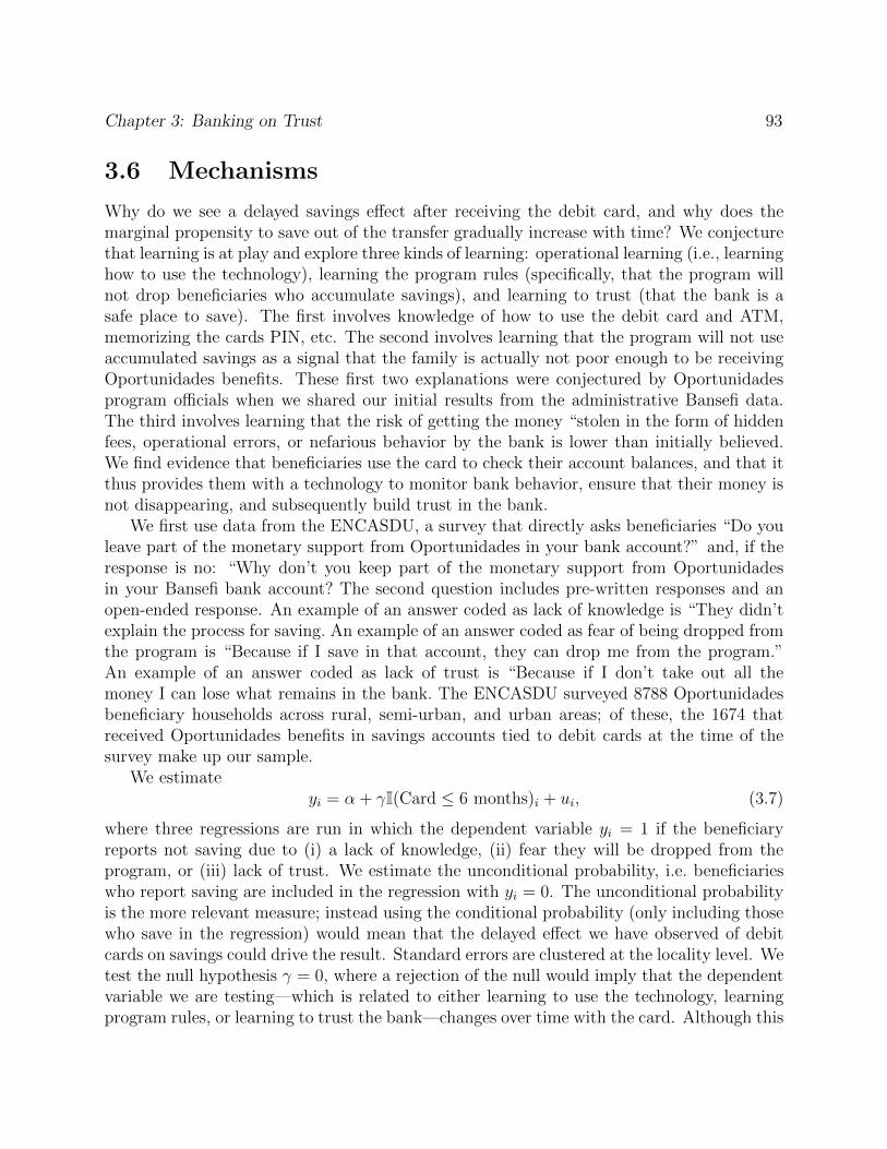
Chapter 3: Banking on Trust 93
3.6 Mechanisms
Why do we see a delayed savings e↵ect after receiving the debit card, and why does themarginal propensity to save out of the transfer gradually increase with time? We conjecturethat learning is at play and explore three kinds of learning: operational learning (i.e., learninghow to use the technology), learning the program rules (specifically, that the program willnot drop beneficiaries who accumulate savings), and learning to trust (that the bank is asafe place to save). The first involves knowledge of how to use the debit card and ATM,memorizing the cards PIN, etc. The second involves learning that the program will not useaccumulated savings as a signal that the family is actually not poor enough to be receivingOportunidades benefits. These first two explanations were conjectured by Oportunidadesprogram o�cials when we shared our initial results from the administrative Bansefi data.The third involves learning that the risk of getting the money “stolen in the form of hiddenfees, operational errors, or nefarious behavior by the bank is lower than initially believed.We find evidence that beneficiaries use the card to check their account balances, and that itthus provides them with a technology to monitor bank behavior, ensure that their money isnot disappearing, and subsequently build trust in the bank.
We first use data from the ENCASDU, a survey that directly asks beneficiaries “Do youleave part of the monetary support from Oportunidades in your bank account?” and, if theresponse is no: “Why don’t you keep part of the monetary support from Oportunidadesin your Bansefi bank account? The second question includes pre-written responses and anopen-ended response. An example of an answer coded as lack of knowledge is “They didn’texplain the process for saving. An example of an answer coded as fear of being dropped fromthe program is “Because if I save in that account, they can drop me from the program.”An example of an answer coded as lack of trust is “Because if I don’t take out all themoney I can lose what remains in the bank. The ENCASDU surveyed 8788 Oportunidadesbeneficiary households across rural, semi-urban, and urban areas; of these, the 1674 thatreceived Oportunidades benefits in savings accounts tied to debit cards at the time of thesurvey make up our sample.
We estimateyi
= ↵ + �I(Card 6 months)i
+ ui
, (3.7)
where three regressions are run in which the dependent variable yi
= 1 if the beneficiaryreports not saving due to (i) a lack of knowledge, (ii) fear they will be dropped from theprogram, or (iii) lack of trust. We estimate the unconditional probability, i.e. beneficiarieswho report saving are included in the regression with y
i
= 0. The unconditional probabilityis the more relevant measure; instead using the conditional probability (only including thosewho save in the regression) would mean that the delayed e↵ect we have observed of debitcards on savings could drive the result. Standard errors are clustered at the locality level. Wetest the null hypothesis � = 0, where a rejection of the null would imply that the dependentvariable we are testing—which is related to either learning to use the technology, learningprogram rules, or learning to trust the bank—changes over time with the card. Although this

Chapter 3: Banking on Trust 94
survey is cross-sectional, we exploit the variation in time with the debit card, exogenouslydetermined by the staggered locality-level rollout of the cards.
Figure 3.12a and Table 3.2a show the results. The first thing to note is that lack ofknowledge and fear of being dropped from the program after saving are rarely cited asreasons for not saving (combined, less than 4 percent of the sample who have had the cardfor less than 6 months do not save for these reasons), while lack of trust is cited by 27percent of those who have had the card for less than 6 months. Second, the proportion whoreport not saving due to a lack of knowledge does not change over time; in contrast, trustincreases gradually with experience: beneficiaries with more than 6 months with the cardare 36 percent less likely to report not saving due to low trust than those with less than 6months with the card.
Next, we explore mechanisms behind operational learning and learning to trust the bankusing the 2012 Payment Methods Survey. The survey includes a number of questions relatedto operational learning: “What have been the main problems you have had with the ATM?;“In general, does someone help you use the ATM?; “Do you know your PIN by heart?;“Did they tell you that with the card you have a Bansefi savings account? It also includesa question on balance checking (“In the last bimester, how many times did you check yourbalance?), which is a mechanism that beneficiaries could use to build trust in the bank oncethey have a debit card. The Payment Methods Survey included 5381 households, drawnby stratified (by payment method and locality) random sampling from all Oportunidadesbeneficiaries; of these, our sample is made up of the 1641 who received their benefits on debitcards tied to savings accounts.
We again use specification (3.7), with yi
equal to: (i) the self-reported number of balancechecks over the past bimester; (ii) the self-reported number of balance checks over the pastbimester without withdrawing any money, constructed as the total number of balance checksminus the number of withdrawals; and dummies if the respondent reports (iii) it is hard touse the ATM; (iv) she gets help using the ATM; (v) she knows her PIN; (vi) she knows shecan save in the account. Because this survey was conducted in 2012, those with the card forat least 6 months now include both wave 1 and wave 2, while beneficiaries in the localitieswe treat as control localities throughout this paper make up the group with cards for lessthan 6 months.
Figure 3.12b and Table 3.2b show the results. Both the number of balance checks andnumber of balance checks without withdrawing decrease over time with the card. Makingtrips to the ATM specifically to check the account balance (i.e., making a balance checkwithout withdrawing any money) decreases by 36 percent after six months compared to thefirst 6 months (from an average of 0.53 balance checks without withdrawing to an averageof 0.34), while most measures that indicate knowledge of how to use the technology do notchange over time: the proportions who report it is hard to use the ATM (around 10 percent),that they get help using the ATM (55 percent), and that they know they can save in theaccount (32 percent) do not change, although there is a statistically significant increase inthe proportion who know their PINs (from 49 to 58 percent).
Finally, we use the administrative transactions data from the 342,709 Bansefi accounts,

Chapter 3: Banking on Trust 95
which include the date, time, and fee charged for each balance check at an ATM for eachaccount, to investigate whether the mechanism that appears to be driving the increase intrust—balance checks which clients use to monitor and, over time, build trust in the bank—holds true in the administrative data; the increased power we have from a large number ofobservations in the administrative data allows us to take a more granular look at balancechecks over time. Note that balance checks at a Bansefi branch are possible both before andafter receiving the debit card. Nevertheless, if the distance to the nearest bank branch ishigh, the debit cards provide a technology that greatly reduces the cost of balance checking(by enabling clients to check their balances at the closest ATM of any bank). Since balancechecks at a Bansefi branch are not charged a fee—unlike balance checks at ATMs in Mexico—we do not observe them in our data, which is why average balance checks (at ATMs) in thegraph begin after debit card receipt.
Figure 3.13 plots the number of times people check their balance per bimester, withvertical lines indicating the timing of card receipt. Again due to the shifting of some paymentsto the end of the previous bimester (which might a↵ect the bimester timing of balancechecks), we continue grouping adjacent bimesters into four-month periods. We observe thatthe number of balance checks per bimester is initially around 2.5 checks on average in wave1 and 1.5 checks on average in wave 2, but in both waves decreases during each four-monthperiod after beneficiaries receive the card, consistent with the trust-building hypothesis. Thisis consistent with the learning to trust hypothesis: through checking her balance, the clientlearns that her money is still in the account and updates downward her belief about the riskof losing money. With simple Bayesian learning, balance checking has decreasing marginalbenefit and she therefore checks her balance less over time.12
3.7 Increase in Overall Savings vs. Substitution
The increase in formal Bansefi account savings might come at the expense of other typesof savings that the household is already conducting, in such a way that total savings isnot a↵ected. The question of whether the observed increase in Bansefi savings crowds outother saving is relevant not only if one is concerned with total household savings, but alsoto understand the mechanics through which the e↵ect on formal savings is operating and asa first step towards thinking about the broader welfare implications of providing a formalsavings account with a debit card.
Does the provision of the debit card and the resulting increase in formal savings repre-sent an increase in overall savings, or is it merely a substitution from other forms of saving?To address this question, we use Oportunidades ENCELURB panel survey, conducted infour waves during the years 2002, 2003, 2004 and November 2009 to 2010. This survey is
12The operational learning hypothesis makes a di↵erent prediction regarding the evolution of balancechecks over time: since it becomes easier—less costly—for a beneficiary to check her balance as she learnsto use the technology (e.g., by memorizing her PIN or learning how to use the ATM), if anything we mightexpect her to check her balance more over time if operational learning were the mechanism at play.

Chapter 3: Banking on Trust 96
conducted by Oportunidades and has comprehensive modules on consumption, income, andassets for 6272 households in urban and semi-urban areas.13 Of the 6272 households in thepost-treatment wave of ENCELURB, 2951 live in urban areas and, according to admin-istrative data provided by Oportunidades and merged with the survey, are Oportunidadesbeneficiaries when interviewed in the post-treatment wave and receive their benefits in a sav-ings account (with or without a debit card); this is the sample used in our analysis, exceptin the placebo tests described in Section 3.9.
As before, we use a DID strategy where we examine changes in consumption, savings, andincome across beneficiaries, exploiting the di↵erential timing of debit card receipt. Becausethe ENCELURB was conducted after wave 1 localities had received cards but before wave2 or control localities had received cards, we compare those with cards (wave 1) to thosewho have not yet received cards (waves 2 and control), respectively referring to them as“treatment and “control in this section of the paper. The identification assumption is thatin the absence of the debit card, treatment and control groups would have experiencedsimilar changes in consumption, income, and assets. We formally test for parallel trends inSection 3.9, and since we indeed find that trends were parallel prior to treatment, we now testwhether there was an increase in savings, which we construct as income minus consumptionfrom the income and consumption modules of ENCELURB. We estimate
yit
= �i
+ �t
+ �Dj(i)t + ⌫
it
(3.8)
separately for five dependent variables: consumption, income, savings (constructed as incomeminus consumption), purchase of durables, and an asset index. All variables except assets aremeasured in pesos per month, i indexes households, and t indexes survey years. As before, allvariables are winsorized at the 5% level (i.e., the 95th percentile, and also the 5th percentilein the case of variables that do not have a lower bound of 0) to avoid results driven byoutliers. The asset index dependent variable is constructed as the first principal componentof dummy variables indicating ownership of the assets that are included in all rounds of thesurvey questionnaire: car, truck, motorcycle, TV, video or DVD player, radio, washer, gasstove and refrigerator. Time-invariant di↵erences in household observables and unobservablesare captured by the household fixed e↵ect �
i
, common time shocks are captured by the timefixed e↵ects �
t
, and Dj(i)t = 1 if locality j in which household i lived prior to treatment has
received debit cards by time t; i.e., in the notation used in specifications (3.1) and (3.6),D
j(i)t ⌘ Tj(i) ⇥ I(t = 2009–10). We use the locality of residence prior to treatment to avoid
capturing migration e↵ects in our estimation and estimate cluster-robust standard errors atthe locality level.
13The 2002, 2003, and 2004 waves had around 17,000 households, but due to budget constraints thenumber of localities was cut for the 2009-2010 wave. The consumption, income, and assets modules ofOportunidades’ analogous survey for rural areas have been used by Angelucci and De Giorgi (2009), Attanasioet al. (2013), Janvry et al. (2015), Gertler, Martinez, and Rubio-Codina (2012), and Hoddinott and Skoufias(2004), while these modules from the ENCELURB have been used by Angelucci and Attanasio (2013) andBehrman et al. (2012).

Chapter 3: Banking on Trust 97
If the increase in formal savings constitutes an increase in total savings then we expect� > 0 for total savings (defined as income minus consumption), and if we observe � = 0for income we expect � < 0 for consumption. If there is no substitution of savings fromassets (and if they are not using the formal savings accounts to save up for assets, at leastin the short run), we expect � = 0 for the purchase of durables (which measures a flow)and the asset index (which measures a stock). This is indeed what we find. Figure 3.15shows that consumption decreased by about 130 pesos on average (statistically significantat the 10% level). Meanwhile, there is no e↵ect on income; we also test the di↵erence in thecoe�cients of consumption and income using a stacked regression (which is equivalent toseemingly unrelated regression when the same regressors are used in each equation, as is thecase here); although both are noisily measured, the di↵erence in the coe�cients is significantat the 10% level (p = 0.072). Purchase of durables and the stock of assets do not change,ruling out a crowding out of these forms of saving. The increase in savings, measured asincome minus consumption—which, although a crude measure of savings, is commonly used(e.g., Dynan, Skinner, and Zeldes 2004)—is estimated at slightly more than 200 pesos, andis significant at the 5% level.
The results in Figure 3.15 are from our main specification where we winsorize the depen-dent variable at 5 percent (specifically, at the 95th percentile, as well as the 5th percentile ifthe variable does not have a lower bound of 0). Appendix Table 3.6, columns 1–3 show thatthe e↵ects are robust to using the raw data without winsorizing, winsorizing at 1 percent,or—as in our main specification—winsorizing at 5 percent (we follow Kast and Pomeranz(2014) and others who show the robustness of results to these three possibilities). They arealso robust to including baseline characteristics interacted with time fixed e↵ects, as wellas municipality-specific time e↵ects, both to control for specific time trends more flexibly(Appendix Table 3.6 columns 4 and 5).14
These results mean that total savings—not just formal savings—increase, and that atleast a substantial portion of this increase in being funded by lower consumption. A back ofthe envelope calculation reveals that the magnitude of the increase in monthly savings fromthis household survey is in line with the average increase of savings in the account from theadministrative data: from the propensity to save specification, after 1 year, beneficiaries whoreceived cards in wave 1 save 26.8% of their transfer more than the control group. UsingENCELURB, transfers are, on average, 20.2% of income for the treatment group, implyingthat the savings e↵ect in the Bansefi administrative data is about 5.4% of income. The e↵ectfor savings (income minus consumption) in the ENCELURB household survey data shown
14The household characteristics interacted with time fixed e↵ects in this robustness check are measured atbaseline and include characteristics of the household head (whether the household head worked, a quadraticpolynomial in years of schooling, and a quadratic polynomial in age), whether the household has a bankaccount, variables used to measure poverty by Oportunidades (the proportion of household members withhealth insurance, the proportion aged 15 or older that are illiterate, the proportion aged 6 to 14 that do notatted school, the proportion aged 15 or older with incomplete primary education, and the proportion aged15 to 29 with less than 9 years of schooling), and dwelling characteristics (dirt floor, no bathroom, no water,no sewage, number of occupants per room).

Chapter 3: Banking on Trust 98
in Figure 13 equates to 4.9% of income. Taken at face value, this suggests that most of theincrease in savings in the account is new saving. This result is consistent with other studieswhere formal savings products were o↵ered, which found that the increased savings in theseproducts did not crowd out other forms of saving (Ashraf, Karlan, and Yin 2015; Dupas andRobinson 2013a; Kast, Meier, and Pomeranz 2012).
3.8 Does Money Burn a Hole in Your Pocket?
Because the accounts pay no interest, but there was clearly an unmet demand for savingsamong program beneficiaries, we explore why they were not able to save before (for exam-ple, under the mattress). Since the results in Figure 3.15 show that the debit card induceshigher total savings through decreased consumption, we might expect that it influences dif-ferent components of consumption di↵erentially. We thus examine the proportion of incomespent on several categories of consumption goods, listed in order of average budget share:meat, dairy, and produce; tortillas and cereals; health and education; transportation; fatsand sweets (junk food, fats, soda); temptation goods (where we group the three most fre-quently cited temptation goods in Banerjee and Mullainathan (2010): alcohol, tobacco, andsugar); and entertainment. We use the proportion of total income spent on each consump-tion category, rather then the level of consumption in that category, because individual ⇥time-specific shocks to income, which we expect to be passed through as shocks to variousconsumption categories, would otherwise add noise to the estimation through the error term;we use total income rather than total consumption in the denominator because, from theresults in Figure 3.15, total income does not change di↵erentially between the treatment andcontrol groups.
We estimate a DID specification with household and year fixed e↵ects and standard errorsclustered at the locality level; specifically, for each consumption category g,
Consumptiongit
Incomeit
= �gi
+ �gt
+ �g
Dj(i)t + ⌫
git
, (3.9)
where Consumptiongit
is monthly consumption of goods category g by household i at time t(in pesos) and Income
it
is total monthly income of household i at time t (in pesos). We findthat the only category of goods in which the treatment group shows a statistically significantdecrease relative to the control is that of temptation goods (Figure 3.16).15 More specifically,the treatment group reduces the proportion of income it spends on temptation goods by 20%relative to the control group. Nevertheless, as the thick horizontal bars in Figure 3.16 show,and as we would expect, only a small portion of income is spent on temptation goods atbaseline (3%). As a result, the statistically significant reduction in spending on temptation
15The whiskers in Figure 3.16 show the 95% confidence intervals when no adjustment is made for multiplehypothesis testing. After adjusting for multiple hypothesis testing using the sharpened false discovery rate(Benjamini, Krieger, and Yekutieli 2006; Anderson 2008), the result for temptation goods is significant atthe 10% rather than 5% level (p = 0.023, q = 0.086).

Chapter 3: Banking on Trust 99
goods only explains 16% of the total e↵ect of the debit cards on consumption. We refrainfrom attempting to determine what categories explain the remaining 84% of the e↵ect sincethe results for other spending categories are not statistically significant.
Although our grouping of temptation goods is based on the goods most frequently men-tioned by Banerjee and Mullainathan (2010), it could be viewed as arbitrary (and, indeed,we do not find a decrease in the grouping of fats and sweets—junk food, fats, and soda—which could also be classified as temptation goods); we thus look separately at each item inthe temptation good category, and find a statistically significant decrease in consumption ofalcohol and sugar, but not of tobacco.
We interpret this result as evidence that it is di�cult to save informally due to self-control problems, and that these problems can be partially solved by access to a formalsavings account (but that low indirect transaction costs and trust in the bank are necessaryconditions for these formal savings accounts to be used). This finding is consistent with thedemand for commitment savings devices (e.g., Ashraf, Karlan, and Yin 2006; Bryan, Karlan,and Nelson 2010) if the savings accounts without debit cards, which could be used as aneven stronger commitment due to the high indirect cost of accessing savings, would havebeen too strong of a commitment (since strong commitment devices have low take-up andlow use relative to weak commitment devices: see Karlan and Linden 2014; Laibson 2015),or if the bank accounts were merely not trusted prior to being able to cheaply monitor themwith debit cards. Under either explanation, trust appears to have been a necessary conditionfor formal saving, given the delayed savings e↵ect and self-reported reasons for not savinginitially.
The self-control problems that prevent the poor from saving prior to having access to atrusted formal savings account could result directly from an asset-based poverty trap, as inBernheim, Ray, and Yeltekin (2015), a model that is consistent with the empirical findingthat microcredit decreases temptation good consumption (Angelucci, Karlan, and Zinman2015; Augsburg et al. 2015; Banerjee et al. 2015). Alternatively, it is possible that the self-control problems stem from the timing of access to the money: Carvalho, Meier, and Wang(2016), using exogenous variation in the timing of an experiment relative to payday, findthat those who are more financially constrained behave in a more present-biased way. If thebeneficiary withdraws her money and attempts to save at home, she has easy access to itthroughout the two month period (including access to the portion she intended to save ratherthan spend that period); toward the end of the period she is likely to be more financiallyconstrained and thus behave in a more present-biased way. On the contrary, if she truststhe bank and decides to save in her Bansefi account, she makes her saving decision wheninitially withdrawing benefits, when she is less financially constrained due to having recentlyreceived the Oportunidades payment.
It is also possible that saving money informally is di�cult because the beneficiary lackscontrol over her husband or partner’s access to money saved at home, and the husbandhas di↵erent (perhaps more present-biased) time preferences. Anderson and Baland (2002,p. 963) present evidence that participation in rotating savings and credit associations “is astrategy a wife employs to protect her savings against claims by her husband for immediate
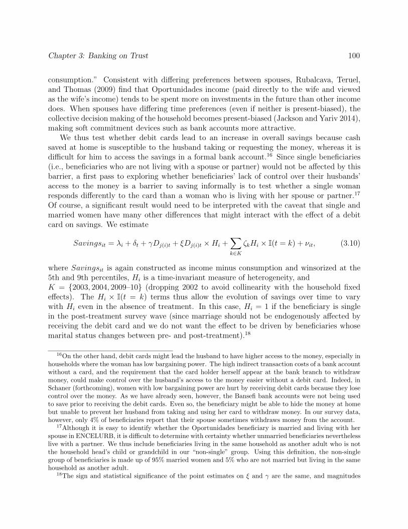
Chapter 3: Banking on Trust 100
consumption.” Consistent with di↵ering preferences between spouses, Rubalcava, Teruel,and Thomas (2009) find that Oportunidades income (paid directly to the wife and viewedas the wife’s income) tends to be spent more on investments in the future than other incomedoes. When spouses have di↵ering time preferences (even if neither is present-biased), thecollective decision making of the household becomes present-biased (Jackson and Yariv 2014),making soft commitment devices such as bank accounts more attractive.
We thus test whether debit cards lead to an increase in overall savings because cashsaved at home is susceptible to the husband taking or requesting the money, whereas it isdi�cult for him to access the savings in a formal bank account.16 Since single beneficiaries(i.e., beneficiaries who are not living with a spouse or partner) would not be a↵ected by thisbarrier, a first pass to exploring whether beneficiaries’ lack of control over their husbands’access to the money is a barrier to saving informally is to test whether a single womanresponds di↵erently to the card than a woman who is living with her spouse or partner.17
Of course, a significant result would need to be interpreted with the caveat that single andmarried women have many other di↵erences that might interact with the e↵ect of a debitcard on savings. We estimate
Savingsit
= �i
+ �t
+ �Dj(i)t + ⇠D
j(i)t ⇥Hi
+X
k2K
⇣k
Hi
⇥ I(t = k) + ⌫it
, (3.10)
where Savingsit
is again constructed as income minus consumption and winsorized at the5th and 9th percentiles, H
i
is a time-invariant measure of heterogeneity, andK = {2003, 2004, 2009–10} (dropping 2002 to avoid collinearity with the household fixede↵ects). The H
i
⇥ I(t = k) terms thus allow the evolution of savings over time to varywith H
i
even in the absence of treatment. In this case, Hi
= 1 if the beneficiary is singlein the post-treatment survey wave (since marriage should not be endogenously a↵ected byreceiving the debit card and we do not want the e↵ect to be driven by beneficiaries whosemarital status changes between pre- and post-treatment).18
16On the other hand, debit cards might lead the husband to have higher access to the money, especially inhouseholds where the woman has low bargaining power. The high indirect transaction costs of a bank accountwithout a card, and the requirement that the card holder herself appear at the bank branch to withdrawmoney, could make control over the husband’s access to the money easier without a debit card. Indeed, inSchaner (forthcoming), women with low bargaining power are hurt by receiving debit cards because they losecontrol over the money. As we have already seen, however, the Bansefi bank accounts were not being usedto save prior to receiving the debit cards. Even so, the beneficiary might be able to hide the money at homebut unable to prevent her husband from taking and using her card to withdraw money. In our survey data,however, only 4% of beneficiaries report that their spouse sometimes withdraws money from the account.
17Although it is easy to identify whether the Oportunidades beneficiary is married and living with herspouse in ENCELURB, it is di�cult to determine with certainty whether unmarried beneficiaries neverthelesslive with a partner. We thus include beneficiaries living in the same household as another adult who is notthe household head’s child or grandchild in our “non-single” group. Using this definition, the non-singlegroup of beneficiaries is made up of 95% married women and 5% who are not married but living in the samehousehold as another adult.
18The sign and statistical significance of the point estimates on ⇠ and � are the same, and magnitudes
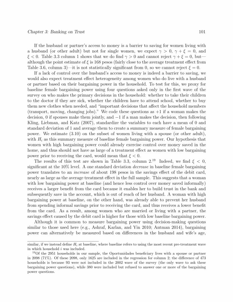
Chapter 3: Banking on Trust 101
If the husband or partner’s access to money is a barrier to saving for women living witha husband (or other adult) but not for single women, we expect � > 0, � + ⇠ = 0, and⇠ < 0. Table 3.3 column 1 shows that we do find � > 0 and cannot reject � + ⇠ = 0, but—although the point estimate of ⇠ is 168 pesos (fairly close to the average treatment e↵ect fromTable 3.6, column 3)—it is not statistically significant from 0, so we cannot reject ⇠ = 0.
If a lack of control over the husband’s access to money is indeed a barrier to saving, wewould also expect treatment e↵ect heterogeneity among women who do live with a husbandor partner based on their bargaining power in the household. To test for this, we proxy forbaseline female bargaining power using four questions asked only in the first wave of thesurvey on who makes the primary decisions in the household: whether to take their childrento the doctor if they are sick, whether the children have to attend school, whether to buythem new clothes when needed, and “important decisions that a↵ect the household members(transport, moving, changing jobs).” We code these questions as +1 if a woman makes thedecision, 0 if spouses make them jointly, and �1 if a man makes the decision, then followingKling, Liebman, and Katz (2007), standardize the variables to each have a mean of 0 andstandard deviation of 1 and average them to create a summary measure of female bargainingpower. We estimate (3.10) on the subset of women living with a spouse (or other adult),with H
i
as this summary measure of baseline female bargaining power. Our hypothesis thatwomen with high bargaining power could already exercise control over money saved in thehome, and thus should not have as large of a treatment e↵ect as women with low bargainingpower prior to receiving the card, would mean that ⇠ < 0.
The results of this test are shown in Table 3.3, column 2.19 Indeed, we find ⇠ < 0,significant at the 10% level. A one standard deviation decrease in baseline female bargainingpower translates to an increase of about 198 pesos in the savings e↵ect of the debit card,nearly as large as the average treatment e↵ect in the full sample. This suggests that a womanwith low bargaining power at baseline (and hence less control over money saved informally)receives a larger benefit from the card because it enables her to build trust in the bank andsubsequently save in the account, which is out of reach of her husband. A woman with highbargaining power at baseline, on the other hand, was already able to prevent her husbandfrom spending informal savings prior to receiving the card, and thus receives a lower benefitfrom the card. As a result, among women who are married or living with a partner, thesavings e↵ect caused by the debit card is higher for those with low baseline bargaining power.
Although it is common to measure bargaining power using decision-making questionssimilar to those used here (e.g., Ashraf, Karlan, and Yin 2010; Antman 2014), bargainingpower can alternatively be measured based on di↵erences in the husband and wife’s age,
similar, if we instead define Hi
at baseline, where baseline refers to using the most recent pre-treatment wavein which household i was included.
19Of the 2951 households in our sample, the Oportunidades beneficiary lives with a spouse or partnerin 2098 (71%). Of these 2098, only 1625 are included in the regression for column 2; the di↵erence of 473households is because 93 were not included in the 2002 wave of the survey (the only wave to ask thesebargaining power questions), while 380 were included but refused to answer one or more of the bargainingpower questions.

Chapter 3: Banking on Trust 102
education, literacy, and income. We now test the robustness of our result to measuringbargaining power using these variables, following the method used by Schaner (forthcoming).Specifically, we construct a Kling, Liebman, and Katz (2007) summary measure of proxiedbargaining power based on di↵erences between spouses in these four variables at baseline.We standardize age, years of schooling, a dummy measuring literacy, and the total incomeearned by the beneficiary or her partner to each have a mean of 0 and standard deviationof 1. We then subtract the value of each variable for the husband or partner from thevalue for the beneficiary to create an indicator that is increasing in the woman’s relative“power” in that dimension, then average across the four indicators. We again standardizethe resulting bargaining power proxy so that the regression coe�cient can be interpreted asthe e↵ect of a one standard deviation in female bargaining power on savings. The sampleis again restricted to women who are married or living with a partner.20 The coe�cientunder this alternative specification, shown in Table 3.3, column 3, is slightly lower thanin the first specification (–163 pesos compared to –198) and is not statistically significant.Because the significance of our prior result is marginal and not robust to alternative measuresof bargaining power (although, reassuringly, point estimates retain their sign and remainsimilar in magnitude), and because bargaining power could be correlated with unobservablesthat explain the heterogeneous treatment e↵ect, we interpret the results based on di↵erencesin baseline bargaining power as merely suggestive.
Another potential barrier to saving informally is that money saved at home could be indemand from friends and relatives. It is obvious from Baland, Guirkinger, and Mali (2011)and Jakiela and Ozier (2016) that the desire to conceal money in a savings account to avoiddemands from others extends beyond one’s spouse to friends and relatives. Ideally, we wouldtest whether transfers from the household to other households decreased after receiving thecard; the question on transfers of money to other households was not included in the post-wave survey, however. We thus estimate (3.10) with H
i
as a dummy variable equal to 1 if thehousehold reported giving money to other households at baseline (specifically, in any of thethree pre-treatment waves). Because those with higher demands for money from friends andrelatives are more likely to have H
i
= 1, if this is a barrier to saving informally we expect⇠ > 0. The results of this test, shown in Table 3.3, column 4, are inconclusive: although thepoint estimate on the interaction term is large, at 354 pesos, the standard error is very large,and the e↵ect is statistically insignificant from 0. It is worth noting that only 7% of thesample has H
i
= 1. This suggests that demands for money from relatives and friends mightbe a barrier to saving informally, but—if so—that this barrier only a↵ects a small fractionof Oportunidades recipients.
20The sample includes 141 households less than in the previous specification due to households withmissing values for years of schooling of the beneficiary or her partner.

Chapter 3: Banking on Trust 103
3.9 Robustness
Internal Validity Checks
The identifying assumption for (3.1) and (3.6) is that the beneficiaries that received thedebit card in waves 1 and 2 would have had the same trend in average balances and marginalpropensity to save as the control group in the absence of treatment. While the assumptionis inherently untestable, its plausibility was confirmed by two sets of results presented sec-tions 3.2 and 3.4. First, although the rollout was not random, most means between treatmentand control do not have statistically significant di↵erences; there is a di↵erence, however,in population, transfer amount, and percent of the transfer withdrawn. (For percent of thetransfer withdrawn, the F-test of equality between the three means is rejected, and a test ofequality of wave 1 and the control is rejected, but the test of equality between wave 2 andthe control is not rejected.) More important, average balances follow parallel pre-treatmenttrends in wave 1 and the control prior to wave 1 receiving debit cards, and in wave 2 and thecontrol prior to wave 2 receiving debit cards: this can be seen visually in Figure 3.6 and isformally tested in Section 3.4. The similarity of savings in the treatment and control groupsbefore treatment contrasts sharply with the diverging trends after debit cards are received.The fact that results comparing the control to two waves receiving debit cards in di↵erentyears are similar suggests this is not an artefact of a shock in a particular month or year.
Similarly, the identifying assumption for the household survey panel data results on sav-ings, income, consumption, purchase of durables, and ownership of assets in (3.8) is thatthese variables would have followed parallel trends in the absence of treatment. Figure 3.14shows these parallel trends graphically for the pre-treatment rounds of the survey. In addi-tion, because there are many years between the last pre-treatment ENCELURB survey year(2004) and the year of treatment (2009), we supplement the ENCELURB parallel trendstests with tests using data from the 2004–2008 rounds of the ENIGH, a national income andexpenditure survey used for Mexico’s o�cial poverty measurement. This is a repeated cross-section survey conducted in even years (but additionally conducted in 2005) that sampledbetween 20,000 and 30,000 households during each year in this time frame.
Although the publicly available version of the survey does not include each household’slocality code, which determines whether the household lives in a treatment or control locality,we obtained the locality codes for sampled households from Mexico’s National Institute ofStatistics and Geography. Although Oportunidades receipt is reported in the survey, thereis a large discrepancy between the number of beneficiaries according to the survey (afterexpansion factors are applied) and the number in national accounts (Scott 2014), a problemalso common in developing countries (Meyer, Mok, and Sullivan 2015), so to have su�cientpower for our test we restrict the analysis to the poorest 20 percent of surveyed householdsto proxy for Oportunidades recipients, rather than use self-reported Oportunidades receipt.Again, the parallel trends can be clearly seen visually in Figure 3.14.

Chapter 3: Banking on Trust 104
Alternative Explanations and Placebo Tests
We have argued that the card allows beneficiaries to build trust in the bank by monitoringthe banks activity through balance checks. We now explore alternative explanations forthe observed delayed savings e↵ect and increasing marginal propensity to save over time.First, it could be that accumulating time with the savings account, rather than with thecard, drives the increase over time. Second, while the hypothesis that debit cards increasedtrust through bank monitoring is demand-driven, the e↵ect could be supply-driven if banksoptimally responded to the increased debit card concentration by opening up more ATMsor bank branches in those localities; if such an expansion were gradual, it could explain thedelayed savings e↵ect and increasing marginal propensity to save over time. Third, the e↵ectmight be driven by locality-specific shocks unrelated to the debit cards. Fourth, the debitcards could merely make savings more salient, as in Akbas et al. (2015), by giving beneficiariesa reminder (in the form of an object carried with them) of their savings intentions.
There are a number of reasons that it is unlikely that the e↵ects are driven by experiencewith the savings account leading beneficiaries to learn the benefits of saving, rather thantime with the debit card itself. First, both treatment and control accounts are accumulat-ing time with their savings accounts simultaneously. Second, because the savings accountswere mainly rolled out between 2002 and 2004 (Figure 3.4), most beneficiaries had alreadyaccumulated several years with the account by 2009, when treatment begins. Indeed, themedian date of account opening in our 342,709 accounts is October 18, 2004, and less than5 percent of accounts had existed for less than two years when they received debit cards.Third, our results from Section 3.5 include account fixed e↵ects, so any time-invariant e↵ectof having the account for a longer period of time would be absorbed. Fourth, to test for atime-varying e↵ect of having the account for a longer period of time, we test whether resultsvary when we run the analysis separately for two groups: those who have had the accountfor more vs. less time. We use the median date of account opening to split the accounts intothese two groups, and find that results are very similar. Appendix Figure 3.18 shows theequivalent of Figure 3.11 separately for older accounts (panels (a) and (b)), opened beforethe median date of October 18, 2004, and younger accounts (panels (c) and (d)) opened onor after that date.
A second possible explanation for the increase in savings over time is that banks grad-ually expanded complementary infrastructure in localities where treated beneficiaries live.Depending on the costs of each branch and ATM machine, this could be a profit-maximizingresponse to the increase in the number of debit card holders in treated localities. The in-creasing marginal propensity to save over time could be the result of the staggered expansionof this infrastructure, not increased trust. If this is so, then the increase in savings wouldhave to be reinterpreted not only as the e↵ect of debit cards but of the expansion of thewhole enabling technology. Using quarterly data for each municipality on the number ofbank branches and ATMs for Bansefi and all other banks, we test if there was indeed acontemporaneous expansion of infrastructure and if this was correlated geographically withOportunidades debit card expansion or with savings in our accounts.

Chapter 3: Banking on Trust 105
We first test for a relationship between the rollout of ATM cards and a supply-sideexpansion of banking infrastructure (ATMs and bank branches)21 by estimating:
ymt
= �m
+ �t
+4X
k=�4
�k
Dm,t+k
+ "jt
,
where ymt
is the number of total ATMs, total bank branches, Bansefi ATMs, or Bansefibranches in municipality m in quarter t and D
mt
equals one if at least one locality in munic-ipality m has Oportunidades debit cards in quarter t. We include one year (four quarters) oflags and one year of leads to test for a relationship between bank the debit card rollout andbank infrastructure. For this test, we use data on the number of ATMs and bank branches bybank by municipality by quarter from the Comisin Nacional Bancaria y de Valores (CNBV),from the last quarter of 2008 through the last quarter of 2013 (since the rollout was from2009 to 2012, when what we refer to as control group localities received debit cards). We sep-arately test whether lags of credit card receipt predict banking infrastructure (i.e., whetherthere is a supply-side response to the rollout of debit cards) by testing ��4 = · · · = ��1 = 0and whether leads of credit card receipt predict banking infrastructure (i.e., whether debitcards were first rolled out in municipalities with a recent expansion of banking infrastruc-ture) by testing �1 = · · · = �4 = 0. We find evidence of neither relationship, failing to rejectthe null hypothesis of each test for each of the four dependent variables (Table 3.4).
To rule out locality-specific shocks that could be driving the savings e↵ect, as opposedto the e↵ect being driven by the debit cards, we perform a placebo test using poor non-Oportunidades households in the treated vs. control localities in the ENCELURB data. TheENCELURB initially included households deemed potentially eligible for the Oportunidadesprogram as it was expanded to urban areas; some households did not become beneficiaries(either they were deemed ineligible or did not take up the program). Because these non-beneficiaries were “potentially eligible” for the program to be included in the survey, they aresimilarly (though not quite as) poor compared to the Oportunidades beneficiaries who makeup our main sample. Because they did not receive debit cards during the rollout, due to notbeing Oportunidades beneficiaries, these individuals in treatment and control localities serveas a good placebo test for locality-level shocks. The results are presented in Figure 3.17a.The DID estimates on consumption, income, and savings are all insignificant from 0, althoughdue to the low number of non-Oportunidades beneficiaries in ENCELURB (382 households),the estimates are very noisy. Nevertheless, it is comforting that the point estimates aresubstantially close to 0 relative to the coe�cients from our main sample, and the coe�cientsfor consumption and savings actually have the opposite sign as the coe�cients from the mainregression (shown again in panel (c) for comparison). This suggests that, although the noisyplacebo estimates’ 95% confidence intervals do include the point estimates from our mainsample, locality-level shocks do not explain the observed results.
21We do not test an expansion of point of service (POS) payment terminals because the data on POSterminals by municipality does not begin until 2011, toward the end of our study period.

Chapter 3: Banking on Trust 106
Finally, we test for a salience e↵ect of the cards themselves, where the card—which abeneficiary might carry with her in a wallet or purse—serves as a salient reminder of hersavings goals. In some localities, beneficiaries received their benefits through Bansefi but didnot have access to a Bansefi savings account (and thus had to withdraw all of their moneyeach pay period at a Bansefi branch); in these localities, the government decree requiring allbeneficiaries to receive benefits through a plastic card led to receiving benefits on a pre-paidcard, still without access to a savings account. Again using ENCELURB, we find that inlocalities without savings accounts that switched to a pre-paid card prior to the last round ofthe survey compared to localities without savings accounts that did not switch prior, therewas no di↵erential e↵ect on consumption, income, or savings. These estimates are againnoisier than the results from the main sample (here we have 2300 households), but the DIDcoe�cient from the placebo consumption regression is statistically significant at the 10%level from the coe�cient from the corresponding consumption regression in the full sample.
Alternative Barriers to Saving Informally
An alternative potential barrier to saving informally is that the money risks being stolen ifsaved at home. An anticipated reduction in crime was one of the primary motivations for thechange to debit cards; in the U.S., changing the payment method of cash welfare paymentsto debit cards caused a significant decline in burglary, assault, and larceny (Wright et al.2014). In developing countries, risk of theft has been anecdotally reported as a reason for notsaving at home by cash transfer recipients in the Dominican Republic (Center for E↵ectiveGlobal Action 2015), and is pointed out as a potential mechanism in Malawi by Brune et al.(2016).
To test this hypothesis, we test whether high-crime municipalities—where saving infor-mally would be more di�cult due to risk of theft—have a higher treatment e↵ect. Specifically,we use three measures of crime at the municipal level: crimes recorded, thefts recorded, andhomicides. Crimes and thefts recorded are based on reported crimes and thus su↵er fromreporting bias; nevertheless, total thefts is the variable that likely best represents the riskspeople face if saving informally. These variables come from Mexico’s Executive Secretariatof the National Public Safety System. Homicides come from national vitality records andare thus less susceptible to bias. All crime rates are for the 2008 calendar year, immediatelyprior to the rollout of debit cards. For each of these three measures of crime, we estimate(3.10) where H
i
(or, more precisely, Hm(i)) is either the crime rate per 100,000 in the munic-
ipality m in which household i lives (Table 3.5, columns 1, 3, and 5) or a dummy variableequal to 1 if the crime rate is greater than the median, with the median calculated basedon the municipal crime rates faced by each beneficiary household in our sample (columns 2,4, and 6). If risk of theft is a barrier to saving, we expect ⇠ > 0, i.e., there was a highersavings e↵ect from the debit cards in localities with higher crime and thus greater risk thatinformal savings are stolen. In all specifications, the point estimate on the interaction termis statistically insignificant from 0; in many, it is close to 0; and in the majority, the sign

Chapter 3: Banking on Trust 107
is negative, contrary to our hypothesis. This suggests that risk of theft is not a barrier tosaving informally in our context.
3.10 Conclusion
Although trust in financial institutions is by no means a su�cient condition to enable the poorto save, our findings suggest that it is a necessary condition. A lack of trust in banks couldexplain why a number of studies have found modest e↵ects of o↵ering savings accounts to thepoor, even when these accounts have no fees or minimum balance requirements. Debit cards,a simple technology with high scale-up potential, provided beneficiaries of Mexico’s large-scale cash transfer program Oportunidades with a mechanism to monitor banks by checkingtheir balances at any bank’s ATM; once beneficiaries built trust in banks, they began tosave and their marginal propensity to save increased over time. We find that the observedincrease in formal savings represents an increase in overall savings rather than a substitutionfrom other forms of saving, and that beneficiaries reduce consumption of temptation goods,suggesting that saving informally is di�cult and the use of financial institutions to save helpssolve self-control problems.
The size of the savings e↵ect, at 5% of income after one year with the debit card and10% after two years, is larger than that of studies on various savings interventions such assubsidizing bank fees, increasing interest rates, and providing commitment savings devices.As a result, interventions that enable account holders to monitor banks and increase theirtrust in financial institutions may be a promising avenue to enable the poor to save in theformal financial sector. Debit cards and other forms of mobile money, which are simple,scalable technologies that are gaining traction in many developing countries, could thus bea highly e↵ective means of increasing financial inclusion among millions of government cashtransfer recipients worldwide.

Chapter 3: Banking on Trust 108
Figure 3.1: Low Trust in Banks Around the World
Percent with low trust(60,100](50,60](40,50](28,40][0,28]No data
Source: World Values Survey, Wave 6 (2010–2014).Notes: N = 82,587 individuals in 60 countries. Low trust in banks is defined as “not very much confidence”or “none at all” for the item “banks” in response to the following question: “I am going to name a numberof organizations. For each one, could you tell me how much confidence you have in them: is it a great dealof confidence, quite a lot of confidence, not very much confidence or none at all?” Countries are dividedinto quintiles, with quintile cut-o↵s rounded to the nearest percentage point in the legend. Darker shadesindicate countries with a higher percent of the population reporting low trust in banks.
Figure 3.2: Low Trust in Banks by Education Level in Mexico
No formal education
Incomplete Primary
Complete Primary
Complete Secondary
Complete University
40 50 60 70 80
Percent with low trust in banks
Source: World Values Survey, Mexico, Wave 6 (2012).Notes: N = 1993 individuals. Low trust in banks is defined as “not very much confidence” or “none at all”for the item “banks” in response to the following question: “I am going to name a number of organizations.For each one, could you tell me how much confidence you have in them: is it a great deal of confidence, quitea lot of confidence, not very much confidence or none at all?”

Chapter 3: Banking on Trust 109
Figure 3.3: Cross-Country Comparison of Trust in Banks and Saving in Financial Institutions
ESP
ARG
YEM
LBN
DZA
TUR
DEU
JORPER
CHLGEO
NLDUSA
ROM
UKR
ECU
RUSPOLIRQCOL
ZAF
KAZ
SVN
AZE
BLR
QAT
AUS
KWT
PAK
MEX
BRA
URY
KGZ
RWA
TTO
SWE
MAR
EGY
NGA
NZL
ZWE
UZB
CYP
KOR
BHRARM
GHA
JPN
CHNSGP
IND
MYS
EST
PHL
HKG
THA
−.4
−.2
0
.2
Pro
port
ion that sa
ve in
fin
anci
al i
nst
itutio
ns
(resi
duals
)
−.3 0 .3
Proportion that trust banks (residuals)
Sources: World Values Survey (WVS), Wave 6 (2010–2014); Global Findex; World Development Indicators(WDI).Notes: N = 56 countries. The y-axis plots residuals from a regression of the proportion that save in financialinstitutions (from Global Findex) against controls (average age, education, and perceived income decilefrom WVS, GDP per capita and growth of GDP per capita from WDI). The x-axis plots residuals from aregression against the same controls of the proportion that respond “a great deal of confidence” or “quitea lot of confidence” in response to the WVS question “I am going to name a number of organizations. Foreach one, could you tell me how much confidence you have in them: is it a great deal of confidence, quitea lot of confidence, not very much confidence or none at all?” The solid line shows a kernel-weighted localpolynomial regression, while the gray area shows its 95% confidence interval.

Chapter 3: Banking on Trust 110
Figure 3.4: Timing of Roll-out and Data
(a) Administrative Bank Account Data
0
200,000
400,000
600,000
800,000
1,000,000
Jan
02
Ma
y 0
2S
ep
02
Jan
03
Ma
y 0
3S
ep
03
Jan
04
Ma
y 0
4S
ep
04
Jan
05
Ma
y 0
5S
ep
05
Jan
06
Ma
y 0
6S
ep
06
Jan
07
Ma
y 0
7S
ep
07
Jan
08
Ma
y 0
8S
ep
08
Jan
09
Ma
y 0
9S
ep
09
Jan
10
Ma
y 1
0S
ep
10
Jan
11
Ma
y 1
1S
ep
11
Jan
12
Oportunidades bank accounts without cardsOportunidades bank accounts with cardsBansefi account balances and transactions
(b) Household Survey Data
0
200,000
400,000
600,000
800,000
1,000,000
Jan
02
Ma
y 0
2S
ep
02
Jan
03
Ma
y 0
3S
ep
03
Jan
04
Ma
y 0
4S
ep
04
Jan
05
Ma
y 0
5S
ep
05
Jan
06
Ma
y 0
6S
ep
06
Jan
07
Ma
y 0
7S
ep
07
Jan
08
Ma
y 0
8S
ep
08
Jan
09
Ma
y 0
9S
ep
09
Jan
10
Ma
y 1
0S
ep
10
Jan
11
Ma
y 1
1S
ep
11
Jan
12
Oportunidades bank accounts without cards ENCELURBOportunidades bank accounts with cards ENIGHPayment Methods Survey ENCASDU
Source: Number of Oportunidades bank accounts with cards and without cards by bimester is from admin-istrative data provided by Oportunidades.

Chapter 3: Banking on Trust 111
Figure 3.5: Geographic Coverage and Expansion of Debit Cards
Sources: Administrative data from Oportunidades on timing of debit card receipt by locality and shape filesfrom INEGI.Notes: N = 275 localities (44 in control, 143 in wave 1, 88 in wave 2). The area of each urban localityincluded in the study is shaded according to its wave of treatment. Urban localities that were not includedin the Oportunidades program at baseline or were included in the program but did not pay beneficiariesthrough Bansefi savings accounts are not included in the figure or in our study.
Figure 3.6: Evolution of Average Balances
0
500
1000
1500
2000
Nov
07
Jan 0
8
Mar
08
May
08
Jul 0
8
Sep 0
8
Nov
08
Jan 0
9
Mar
09
May
09
Jul 0
9
Sep 0
9
Nov
09
Jan 1
0
Mar
10
May
10
Jul 1
0
Sep 1
0
Nov
10
Jan 1
1
Mar
11
May
11
Jul 1
1
Sep 1
1
Wave 1Control
(a) Wave 1 vs. Control
0
500
1000
1500
2000
Nov
07
Jan 0
8
Mar
08
May
08
Jul 0
8
Sep 0
8
Nov
08
Jan 0
9
Mar
09
May
09
Jul 0
9
Sep 0
9
Nov
09
Jan 1
0
Mar
10
May
10
Jul 1
0
Sep 1
0
Nov
10
Jan 1
1
Mar
11
May
11
Jul 1
1
Sep 1
1Wave 2Control
(b) Wave 2 vs Control
Sources: Administrative data from Bansefi on average account balances by bimester and timing of cardreceipt.Notes: N = 5,834,468 account-bimester observations from 343,204 accounts. Average balances arewinsorized at the 95th percentile.

Chapter 3: Banking on Trust 112
Figure 3.7: Di↵erence between Treatment and Control in Average Balances
0
500
1000
1500
No
v 0
7−
Fe
b 0
8
Ma
r−Ju
n 0
8
Jul−
Oct
08
No
v 0
8−
Fe
b 0
9
Ma
r−Ju
n 0
9
Jul−
Oct
09
No
v 0
9−
Fe
b 1
0
Ma
r−Ju
n 1
0
Jul−
Oct
10
No
v 1
0−
Fe
b 1
1
Ma
r−Ju
n 1
1
Jul−
Oct
11
(a) Wave 1 vs. Control
0
500
1000
1500
No
v 0
7−
Fe
b 0
8
Ma
r−Ju
n 0
8
Jul−
Oct
08
No
v 0
8−
Fe
b 0
9
Ma
r−Ju
n 0
9
Jul−
Oct
09
No
v 0
9−
Fe
b 1
0
Ma
r−Ju
n 1
0
Jul−
Oct
10
No
v 1
0−
Fe
b 1
1
Ma
r−Ju
n 1
1
Jul−
Oct
11
(b) Wave 2 vs. Control
Sources: Administrative data from Bansefi on average account balances by bimester and timing of cardreceipt.Notes: (a) N = 2,023,862 from 171,441 accounts. (b) N = 3,086,749 from 270,046 accounts. The figureplots �
k
from (3.1).
Figure 3.8: Withdrawal to Deposit Ratio per Bimester
0
.5
1
1.5
2
Nov−
Dec
07
Mar−
Apr
08
Jul−
Aug 0
8
Nov−
Dec
08
Mar−
Apr
09
Jul−
Aug 0
9
Nov−
Dec
09
Mar−
Apr
10
Jul−
Aug 1
0
Nov−
Dec
10
Mar−
Apr
11
Jul−
Aug 1
1
Wave 1Control
(a) Wave 1 vs. Control
0
.5
1
1.5
2
Nov−
Dec
07
Mar−
Apr
08
Jul−
Aug 0
8
Nov−
Dec
08
Mar−
Apr
09
Jul−
Aug 0
9
Nov−
Dec
09
Mar−
Apr
10
Jul−
Aug 1
0
Nov−
Dec
10
Mar−
Apr
11
Jul−
Aug 1
1
Wave 2Control
(b) Wave 2 vs. Control
Sources: Administrative data from Bansefi on transactions by quarter and timing of card receipt.Notes: N = 14,594,799 transactions from 343,204 accounts.
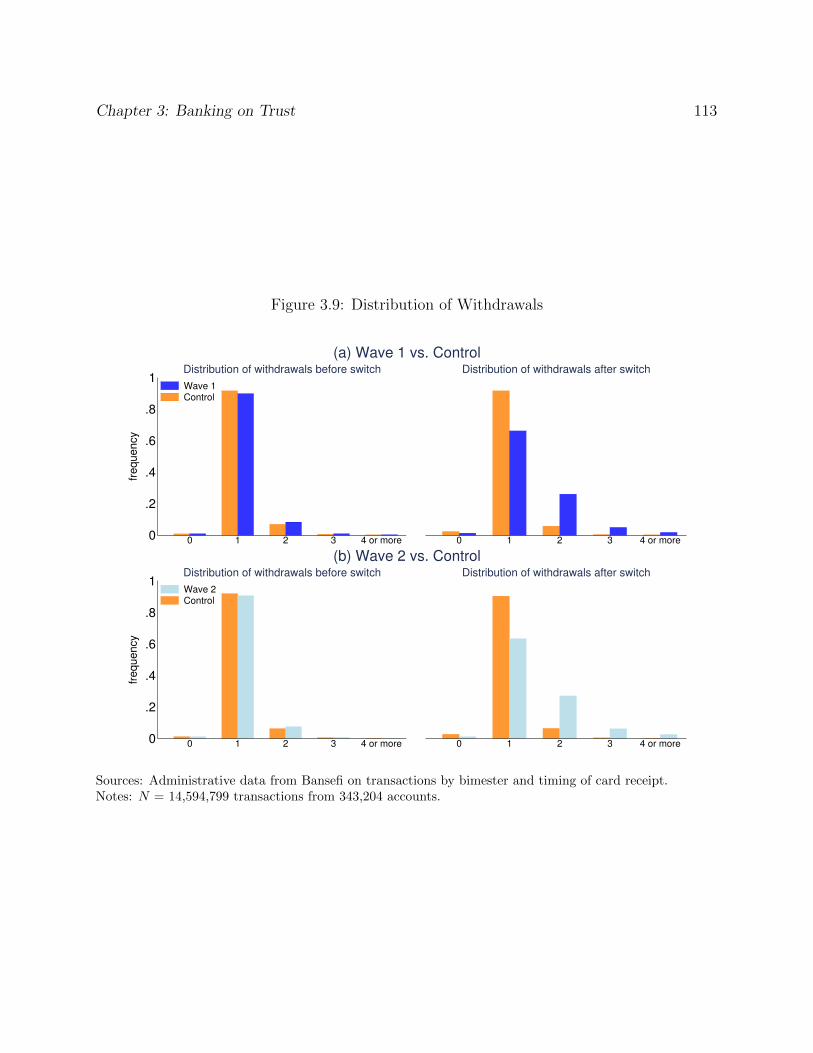
Chapter 3: Banking on Trust 113
Figure 3.9: Distribution of Withdrawals
0
.2
.4
.6
.8
1
fre
qu
en
cy
0 1 2 3 4 or more
Wave 1Control
Distribution of withdrawals before switch
0
.2
.4
.6
.8
1
0 1 2 3 4 or more
Distribution of withdrawals after switch
(a) Wave 1 vs. Control
0
.2
.4
.6
.8
1
fre
qu
en
cy
0 1 2 3 4 or more
Wave 2Control
Distribution of withdrawals before switch
0
.2
.4
.6
.8
1
0 1 2 3 4 or more
Distribution of withdrawals after switch
(b) Wave 2 vs. Control
Sources: Administrative data from Bansefi on transactions by bimester and timing of card receipt.Notes: N = 14,594,799 transactions from 343,204 accounts.

Chapter 3: Banking on Trust 114
Figure 3.10: Di↵erence between Treatment and Control in Net Balances
0
500
1000
No
v 0
7−
Fe
b 0
8
Ma
r−Ju
n 0
8
Jul−
Oct
08
No
v 0
8−
Fe
b 0
9
Ma
r−Ju
n 0
9
Jul−
Oct
09
No
v 0
9−
Fe
b 1
0
Ma
r−Ju
n 1
0
Jul−
Oct
10
No
v 1
0−
Fe
b 1
1
Ma
r−Ju
n 1
1
Jul−
Oct
11
(a) Wave 1 vs. Control
0
500
1000
No
v 0
7−
Fe
b 0
8
Ma
r−Ju
n 0
8
Jul−
Oct
08
No
v 0
8−
Fe
b 0
9
Ma
r−Ju
n 0
9
Jul−
Oct
09
No
v 0
9−
Fe
b 1
0
Ma
r−Ju
n 1
0
Jul−
Oct
10
No
v 1
0−
Fe
b 1
1
Ma
r−Ju
n 1
1
Jul−
Oct
11
(b) Wave 2 vs. Control
Sources: Administrative data from Bansefi on average account balances by bimester, timing and amount oftransfer payments, timing and amount of withdrawals, and timing of card receipt.Notes: (a) N = 2,023,862 from 171,441 accounts. (b) N = 3,086,749 from 270,046 accounts. Net balancesrefer to average balances minus the mechanical e↵ect on average balance of leaving a portion of the depositin the account for a certain number of days before withdrawing it. The figure plots �
k
from (3.1).

Chapter 3: Banking on Trust 115
Figure 3.11: Di↵erence between Treatment and Control in Marginal Propensity to Save Outof Transfer
0.0
0.2
0.4
Ma
r−Ju
n 0
8
Jul−
Oct
08
No
v 0
8−
Fe
b 0
9
Ma
r−Ju
n 0
9
Jul−
Oct
09
No
v 0
9−
Fe
b 1
0
Ma
r−Ju
n 1
0
Jul−
Oct
10
No
v 1
0−
Fe
b 1
1
Ma
r−Ju
n 1
1
Jul−
Oct
11
(a) Wave 1 vs. Control
0.0
0.2
0.4
Ma
r−Ju
n 0
8
Jul−
Oct
08
No
v 0
8−
Fe
b 0
9
Ma
r−Ju
n 0
9
Jul−
Oct
09
No
v 0
9−
Fe
b 1
0
Ma
r−Ju
n 1
0
Jul−
Oct
10
No
v 1
0−
Fe
b 1
1
Ma
r−Ju
n 1
1
Jul−
Oct
11
(b) Wave 2 vs. Control
Sources: Administrative data from Bansefi on average account balances by bimester, timing and amount oftransfer payments, timing and amount of withdrawals, and timing of card receipt.Notes: (a) N = 1,852,416 from 171,441 accounts. (b) N = 2,816,671 from 270,046 accounts. (Total numberof observations does not include the t = 1 observations, which are not included in the regressions butare used to generate y
ij,t�1 for t = 2 observations.) The figure plots ↵k
/µk
+ k
from (3.6) estimatedby Blundell and Bond (1998) two-step system GMM, where µ
k
is average transfers in period k. Averagebalances and transfer amounts are winsorized at the 95th percentile within the treatment and controlgroups and within each time period. The variance of ↵k
µk+
k
is estimated using the delta method.

Chapter 3: Banking on Trust 116
Figure 3.12: Trust and Knowledge Over Time with the ATM Card
(a) ENCASDU (2010)
**
0
.1
.2
.3
.4
Lack of knowledge Fear of ineligibility Lack of trust
Debit card < 6 monthsDebit card > 6 months
Does not save in Bansefi account due to
(b) Payment Methods Survey (2012)
** **
0
.5
1
1.5
Balancechecks
Checkswithout
withdrawing
Building trust
**
0
.2
.4
.6
Hard touse ATM
Gets helpusing ATM
KnowsPIN
Knows cansave inaccount
Learning the technology
Debit card < 6 monthsDebit card > 6 months
Sources: ENCASDU 2010 and Payment Methods Survey 2012.Notes: (a) N = 1674. (b) N = 1617, or less in some regressions if there were respondents who reported“don’t know” or refused to respond (see Table 3.2 for number of observations in each regression). Balancechecks are measured over the past bimester. Bars for “debit card < 6 months” are colored light blue in (a)because at the time of ENCASDU 2010, those with the card 6 months or less were in wave 2 localities; barsfor “debit card < 6 months” are colored orange in (b) because at the time of Payment Methods Survey 2012,those with the card 6 months or less were in control localities.

Chapter 3: Banking on Trust 117
Figure 3.13: Balance Checks (Administrative Data)
0
.5
1
1.5
2
2.5
No
v 0
9
Ma
r 1
0
Jul 1
0
No
v 1
0
Ma
r 1
1
Jul 1
1
No
v 1
1
Wave 1
0
.5
1
1.5
2
2.5
No
v 0
9
Ma
r 1
0
Jul 1
0
No
v 1
0
Ma
r 1
1
Jul 1
1
No
v 1
1
Wave 2
Source: Aministrative transactions data from Bansefi.Notes: Number of balance checks per account tied to a debit card. Prior to receiving the card it was possibleto check balances at Bansefi branches only, and balance checks at Bansefi branches are not recorded in ourtransactions data because they are free of charge.
Figure 3.14: Parallel Pre-Treatment Trends in Household Survey Data
(a)
300
400
500
600
700
2002 2003 2004
Year
Control
Treatment
ENCELURB: Pre−Treatment Consumption (pesos/week)
(b)
300
400
500
600
700
2004 2005 2006 2007 2008
Year
Control
Treatment
ENIGH: Pre−Treatment Consumption (pesos/week)

Chapter 3: Banking on Trust 118
Figure 3.15: E↵ect of the debit card on consumption, income, total savings, purchase ofdurables, and assets
*
Purchase of Durables
Savings = Income − Consumption
Income
Consumption
−200 0 200
Pesos per month
Difference in differences estimates
Asset Index
space
−1 0 1
Standard deviations
Sources: ENCELURB panel survey combined with administrative data on timing of card receipt and transferpayment histories for each surveyed beneficiary household.Notes: N = 11, 275 (number of households = 2951).

Chapter 3: Banking on Trust 119
Figure 3.16: E↵ect of the debit card on di↵erent categories of consumption
Entertainment
Alcohol, tobacco, sugar
Junk food, fats, soda
Transportation
Health and education
Tortillas and cereals
Meat, dairy, produce
−60 −40 −20 0 20 40
Percent
Percent change in proportion of income spent on...
Sources: ENCELURB panel survey combined with administrative data on timing of card receipt and transferpayment histories for each surveyed beneficiary household.Notes: N = 11, 275 (number of households = 2951). Each plotted coe�cient is from a separate regressionusing (3.9), and shows the percent change in the proportion of income spent on that category of consumption.In other words, the graph plots �
g
/µg
, where µg
is the mean proportion of income spent on consumptioncategory g by the control group at baseline. Categories are sorted in descending order of the percent ofincome spent on each consumption category at baseline, i.e. 100µ
g
, which is shown by the thick horizontalbars. The whiskers show 95% confidence intervals with no adjustment for multiple hypothesis testing. Afteradjusting for multiple hypothesis testing using the sharpened false discovery rate (Benjamini, Krieger, andYekutieli 2006; Anderson 2008), the result for the “alcohol, tobacco, and sugar” category is significant atthe 10% rather than 5% level (p = 0.023, q = 0.086).

Chapter 3: Banking on Trust 120
Figure 3.17: Placebo Tests
Savings = Income − Consumption
Income
Consumption
−500 −250 0 250 500
Pesos per month
(a) Placebo 1: Poor Non−Beneficiaries
Savings = Income − Consumption
Income
Consumption
−500 −250 0 250 500
Pesos per month
(b) Placebo 2: Pre−Paid Cards
Savings = Income − Consumption
Income
Consumption
−500 −250 0 250 500
Pesos per month
(c) Original Estimates (For Comparison)
Sources: ENCELURB panel survey combined with administrative data on timing of card receipt and transferpayment histories for each surveyed beneficiary household.Notes: (a) N = 1415 (number of households = 382); (b) N = 8862 (number of households = 2300); (c)N = 11, 275 (number of households = 2951).

Chapter 3: Banking on Trust 121
Table 3.1: Comparison of Baseline Means
Variable Control Wave 1 Wave 2 Di↵. Di↵. F-testW1–C W2–C p-value
Panel A: Locality-level dataLog population 10.57 11.18 11.48 0.60⇤⇤⇤ 0.91⇤⇤⇤ 0.000⇤⇤⇤
(0.11) (0.10) (0.16) (0.14) (0.19)Bansefi branches per 100,000 1.27 1.23 1.58 −0.03 0.32 0.411
(0.28) (0.13) (0.23) (0.30) (0.36)% HHs in poverty 15.93 13.20 12.23 −2.73 −3.71⇤ 0.177
(1.67) (0.75) (1.09) (1.82) (1.99)Occupants per room 1.18 1.11 1.12 −0.07 −0.06 0.260
(0.04) (0.01) (0.02) (0.04) (0.04)Number of localities 44 143 88
Panel B: Administrative bank account dataAverage balance 581.25 670.32 614.29 89.07 33.05 0.112
(12.46) (56.24) (21.26) (55.33) (23.95)Number of deposits 1.06 1.05 1.06 −0.02 −0.01 0.907
(0.01) (0.04) (0.03) (0.04) (0.03)Size of transfer 1506.55 1809.50 1761.26 302.96⇤⇤⇤ 254.71⇤⇤⇤ 0.000⇤⇤⇤
(12.73) (20.16) (17.47) (23.67) (21.15)Number of withdrawals 1.03 1.01 1.02 −0.01 −0.01 0.757
(0.01) (0.03) (0.02) (0.03) (0.02)Percent withdrawn 98.56 97.50 99.64 −1.06⇤⇤ 1.08 0.021⇤⇤
(0.18) (0.45) (0.71) (0.46) (0.72)Years with account 5.31 5.49 5.21 0.17 −0.10 0.510
(0.08) (0.15) (0.25) (0.17) (0.26)Number of accounts 97,922 73,070 171,717
Sources: Census (2005), Bansefi branch locations (2008), poverty estimates from Oportunidades (based on2005 Census), timing of card receipt by locality from Oportunidades, and administrative data from Bansefi.Notes: W1 = wave 1, W2 = wave 2, C = control, Di↵. = di↵erence. For the administrative data fromBansefi, baseline is defined as January 2009 to October 2009 (prior to any accounts receiving cards in thedata from Bansefi).

Chapter 3: Banking on Trust 122
Table 3.2: Trust and Knowledge Over Time with the ATM Card
Mean Has card N 6 months
Panel A: ENCASDU Survey (2010): Doesn’t save in Bansefi due to . . .Lack of knowledge 0.017⇤⇤⇤ −0.003 1,674
(0.002) (0.010)Fear of ineligibility 0.019⇤⇤⇤ 0.015 1,674
(0.004) (0.015)Lack of trust 0.175⇤⇤⇤ 0.095⇤⇤ 1,674
(0.012) (0.044)
Panel B: Payment Methods Survey (2012)Lack of trustTimes checked balance 1.146⇤⇤⇤ 0.251⇤⇤ 1,493
(0.039) (0.105)Times checked balance without withdrawing 0.336⇤⇤⇤ 0.190⇤⇤ 1,490
(0.035) (0.093)Lack of knowledgeHard to use ATM 0.106⇤⇤⇤ 0.002 1,617
(0.013) (0.025)Gets help using ATM 0.498⇤⇤⇤ 0.050 1,612
(0.023) (0.048)Knows PIN 0.575⇤⇤⇤ −0.085⇤⇤ 1,609
(0.017) (0.034)Knows can save in account 0.353⇤⇤⇤ −0.034 1,617
(0.023) (0.046)
Notes: ⇤ indicates statistical significance at p < 0.1, ⇤⇤ p < 0.05, and ⇤⇤⇤ p < 0.01. Standard errors areclustered at the locality level. The “Mean” column shows the mean for those who have had the card formore than six months; the “Has card 6 months” column shows the regression coe�cient on a dummyfor those who have had the debit card for six months or fewer (i.e., the di↵erence relative to the meancolumn). The precise questions on trust and knowledge are as follows. In the ENCASDU, the questionsare “Do you leave part of the monetary support from Oportunidades in your bank account?” and, if theresponse is no, “Why don’t you keep part of the monetary support from Oportunidades in your Bansefibank account?” The regressions presented here are not conditional on saving; those who report yes to thefirst question are coded with trust and knowledge dependent variables of 0 and included in the regressions.The second question includes pre-written responses and an open-ended response (“other; specify”; 4% of thesample in this table responded using the open-ended option); both pre-written and open-ended responseswere coded as lack of knowledge, fear of ineligibility, lack of trust, or another explanation for not saving.In the Payment Methods Survey, each regression comes from a di↵erent survey question. These questionsare: (1) Times checked balance: “In the last bimester, how many times did you consult your balance?” (2)Times checked balance without withdrawing: created by subtracting “In the last bimester, how many timesdid you withdraw money from the ATM?” from (1); (3) Hard to use ATM: responded “The ATM is di�cultto use” (pre-written response) or a similar open-ended response to the question “What have been the mainproblems you have had with the ATM? [Wait for a response and record up to three of the options]”; (4) Getshelp using ATM: “In general, does someone help you use the ATM?”; (5) Knows PIN: “Do you know yourPIN by heart?”; (6) Knows can save in account: “Did they tell you that with the card you have a Bansefisavings account?”
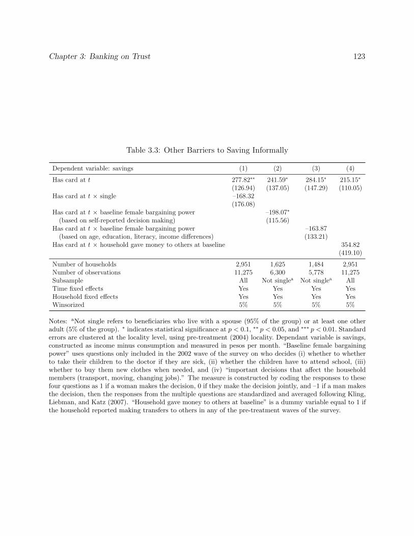
Chapter 3: Banking on Trust 123
Table 3.3: Other Barriers to Saving Informally
Dependent variable: savings (1) (2) (3) (4)
Has card at t 277.82⇤⇤ 241.59⇤ 284.15⇤ 215.15⇤
(126.94) (137.05) (147.29) (110.05)Has card at t ⇥ single –168.32
(176.08)Has card at t ⇥ baseline female bargaining power –198.07⇤
(based on self-reported decision making) (115.56)Has card at t ⇥ baseline female bargaining power –163.87(based on age, education, literacy, income di↵erences) (133.21)
Has card at t ⇥ household gave money to others at baseline 354.82(419.10)
Number of households 2,951 1,625 1,484 2,951Number of observations 11,275 6,300 5,778 11,275Subsample All Not singlea Not singlea AllTime fixed e↵ects Yes Yes Yes YesHousehold fixed e↵ects Yes Yes Yes YesWinsorized 5% 5% 5% 5%
Notes: aNot single refers to beneficiaries who live with a spouse (95% of the group) or at least one otheradult (5% of the group). ⇤ indicates statistical significance at p < 0.1, ⇤⇤ p < 0.05, and ⇤⇤⇤ p < 0.01. Standarderrors are clustered at the locality level, using pre-treatment (2004) locality. Dependant variable is savings,constructed as income minus consumption and measured in pesos per month. “Baseline female bargainingpower” uses questions only included in the 2002 wave of the survey on who decides (i) whether to whetherto take their children to the doctor if they are sick, (ii) whether the children have to attend school, (iii)whether to buy them new clothes when needed, and (iv) “important decisions that a↵ect the householdmembers (transport, moving, changing jobs).” The measure is constructed by coding the responses to thesefour questions as 1 if a woman makes the decision, 0 if they make the decision jointly, and –1 if a man makesthe decision, then the responses from the multiple questions are standardized and averaged following Kling,Liebman, and Katz (2007). “Household gave money to others at baseline” is a dummy variable equal to 1 ifthe household reported making transfers to others in any of the pre-treatment waves of the survey.

Chapter 3: Banking on Trust 124
Table 3.4: Supply-Side Response
Total BansefiATMs Branches ATMs Branches
Current quarter −1.52 0.03 −0.01 −0.01(4.14) (0.30) (0.01) (0.02)
1 quarter lag 0.01 0.02 −0.02 0.02(4.11) (0.34) (0.01) (0.02)
2 quarter lag −10.83 0.08 0.01 0.01(5.64) (0.36) (0.03) (0.01)
3 quarter lag −5.42 0.08 −0.03 0.02(2.98) (0.26) (0.02) (0.02)
4 quarter lag −0.74 0.42 0.00 −0.03(5.97) (0.50) (0.01) (0.03)
1 quarter lead −1.10 −0.12 −0.01 0.00(3.66) (0.36) (0.00) (0.02)
2 quarter lead −6.09 0.25 0.00 0.01(4.90) (0.34) (0.02) (0.01)
3 quarter lead −7.84 0.25 −0.03 −0.01(8.00) (0.65) (0.01) (0.03)
4 quarter lead 7.58 0.59 −0.01 −0.06(10.32) (0.94) (0.03) (0.05)
Mean control group 198.29 36.87 0.49 1.41F-test of lags 1.26 0.20 0.68 0.96[p-value] [0.29] [0.94] [0.61] [0.43]F-test of leads 0.69 0.44 0.79 0.67[p-value] [0.60] [0.78] [0.53] [0.62]
Municipality fixed e↵ects Yes Yes Yes YesQuarter fixed e↵ects Yes Yes Yes Yes
Notes: ⇤ indicates statistical significance at p < 0.1, ⇤⇤ p < 0.05, and ⇤⇤⇤ p < 0.01. The table shows �k
from
yjt
= �j
+ �t
+4X
k=�4
�k
Dj,t+k
+ "jt
where yjt
is the number of ATMs or bank branches of any bank or of Bansefi in municipalityj during quarter t, D
jt
= 1 if municipality j has at least one locality with Oportunidadesdebit cards in quarter t. The F-test of lags tests ��4 = · · · = ��1 = 0; the F-test of leadstests �1 = · · · = �4 = 0.

Chapter 3: Banking on Trust 125
Table 3.5: Crime as a Barrier to Saving Informally
Dependent variable: savings (1) (2) (3) (4) (5) (6)
Has card at t 223.76⇤ 189.63 151.25 153.84 295.98⇤⇤ 268.20⇤
(117.48) (115.45) (117.85) (123.30) (116.74) (135.26)Has card at t ⇥ municipal crimes per 100,000 –0.07
(0.09)Has card at t ⇥ above median crimes per 100,000 –69.63
(206.45)Has card at t ⇥ municipal thefts per 100,000 –0.02
(0.19)Has card at t ⇥ above median thefts per 100,000 59.10
(201.25)Has card at t ⇥ municipal homicides per 100,000 –6.92
(4.46)Has card at t ⇥ above median homicides per 100,000 –165.77
(217.16)
Number of households 2,951 2,951 2,951 2,951 2,951 2,951Number of observations 11,275 11,275 11,275 11,275 11,275 11,275Time fixed e↵ects Yes Yes Yes Yes Yes YesHousehold fixed e↵ects Yes Yes Yes Yes Yes YesWinsorized 5% 5% 5% 5% 5% 5%
Notes: ⇤ indicates statistical significance at p < 0.1, ⇤⇤ p < 0.05, and ⇤⇤⇤ p < 0.01. Standard errors areclustered at the locality level, using pre-treatment (2004) locality. Dependant variable is savings, constructedas income minus consumption and measured in pesos per month.

Chapter 3: Banking on Trust 126
Appendix A: Additional Figures and Tables
Table 3.6: Change in Savings and Assets After Receiving Card
(1) (2) (3) (4) (5)
Consumption –178.76⇤⇤ –144.01⇤ –132.90⇤ –251.28⇤⇤ –149.74⇤⇤
(85.60) (74.76) (67.30) (116.00) (68.58)Income 85.91 106.55 72.16 40.93 69.71
(158.58) (138.41) (123.88) (137.48) (122.05)P-value Consumption vs. Income [0.055]⇤ [0.033]⇤⇤ [0.071]⇤ [0.008]⇤⇤⇤ [0.053]⇤
Savings = Income – Consumption 264.66⇤ 241.30⇤⇤ 215.98⇤⇤ 285.42⇤⇤ 234.59⇤⇤
(134.64) (114.94) (103.50) (118.95) (104.74)Purchase of durables 5.94 6.22 7.99 6.55 6.91
(12.55) (8.52) (4.82) (6.78) (4.55)Asset index 0.04 0.04 0.06 –0.07 0.05
(0.07) (0.07) (0.06) (0.06) (0.06)
Number of households 2,951 2,951 2,951 2,951 2,938Number of observations 11,275 11,275 11,275 11,275 11,243Time fixed e↵ects Yes Yes Yes Yes YesHousehold fixed e↵ects Yes Yes Yes Yes YesMunicipality ⇥ time fixed e↵ects No No No Yes NoHousehold characteristics ⇥ time No No No No YesWinsorized No 1% 5% 5% 5%
Notes: ⇤ indicates statistical significance at p < 0.1, ⇤⇤ p < 0.05, and ⇤⇤⇤ p < 0.01. Standard errors areclustered at the locality level, using pre-treatment (2004) locality. Dependant variables are measured inpesos per month, with the exception of the asset index. Asset index is the first principal component ofassets that are included in both the early (2002, 2003, 2004) and post-treatment (2009–2010) versions ofthe survey: car, truck, motorcycle, television, video or DVD player, radio or stereo, washer, gas stove,and refrigerator. Household characteristics are measured at baseline (2004, or for households that were notincluded in the 2004 wave, 2003). They include characteristics of the household head (working status, aquadratic polynomial in years of schooling, and a quadratic polynomial in age), whether anyone in thehousehold has a bank account, a number of characteristics used by the Mexican government to target socialprograms (the proportion of household members with access to health insurance, the proportion age 15 andolder that are illiterate, the proportion ages 6-14 that do not attend school, the proportion 15 and older withincomplete primary education, the proportion ages 15-29 with less than 9 years of schooling), and dwellingcharacteristics (dirt floors, no bathroom, no piped water, no sewage, and number of occupants per room).The number of households in column (5) is slightly lower because 13 households have missing values for oneof the household characteristics included (interacted with time fixed e↵ects) in that specification.
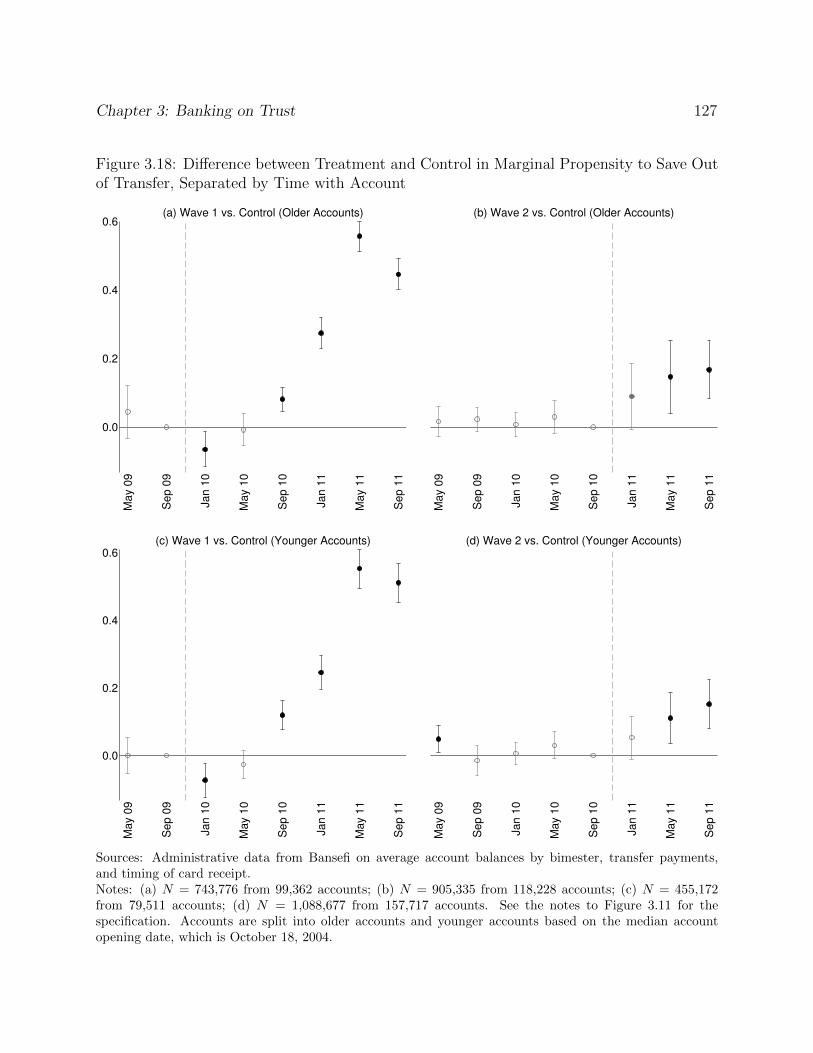
Chapter 3: Banking on Trust 127
Figure 3.18: Di↵erence between Treatment and Control in Marginal Propensity to Save Outof Transfer, Separated by Time with Account
0.0
0.2
0.4
0.6
Ma
y 0
9
Se
p 0
9
Jan
10
Ma
y 1
0
Se
p 1
0
Jan
11
Ma
y 1
1
Se
p 1
1
(a) Wave 1 vs. Control (Older Accounts)
0.0
0.2
0.4
0.6
Ma
y 0
9
Se
p 0
9
Jan
10
Ma
y 1
0
Se
p 1
0
Jan
11
Ma
y 1
1
Se
p 1
1
(b) Wave 2 vs. Control (Older Accounts)
0.0
0.2
0.4
0.6
Ma
y 0
9
Se
p 0
9
Jan
10
Ma
y 1
0
Se
p 1
0
Jan
11
Ma
y 1
1
Se
p 1
1
(c) Wave 1 vs. Control (Younger Accounts)
0.0
0.2
0.4
0.6
Ma
y 0
9
Se
p 0
9
Jan
10
Ma
y 1
0
Se
p 1
0
Jan
11
Ma
y 1
1
Se
p 1
1
(d) Wave 2 vs. Control (Younger Accounts)
Sources: Administrative data from Bansefi on average account balances by bimester, transfer payments,and timing of card receipt.Notes: (a) N = 743,776 from 99,362 accounts; (b) N = 905,335 from 118,228 accounts; (c) N = 455,172from 79,511 accounts; (d) N = 1,088,677 from 157,717 accounts. See the notes to Figure 3.11 for thespecification. Accounts are split into older accounts and younger accounts based on the median accountopening date, which is October 18, 2004.

Chapter 3: Banking on Trust 128
Appendix B: Mechanical E↵ect
This appendix explains the computation of the mechanical e↵ect for every pattern of depositand withdrawal that occurs in a bimester. The mechanical e↵ect is defined as the contributionto average balances from the transit of the Opportunidades transfers on recipients’ accounts,and interpreted as the part of average balances that does not represent net savings in thebimester.
Table 3.7: Computation of Mechanical E↵ect
Pattern % Total Conditions Mechanical E↵ect
Panel A. Regular patterns: single deposit into account in the bimester(1) DW 73.4% W D lapse
DW
⇤WithdrawalW > D lapse
DW
⇤Deposit
(2) DWW 9.1% W1 � D lapseDW1 ⇤Deposit
W1 < D & W1 +W2 � D lapseDW1 ⇤Withdrawal1 + lapse
DW2 ⇤ (Deposit�Withdrawal1)W1 +W2 < D lapse
DW1 ⇤Withdrawal1 + lapseDW2 ⇤ (Withdrawal2)
(3) DWWW 1.7% W1 � D lapseDW1 ⇤Deposit
W1 < D & W1 +W2 � D lapseDW1 ⇤Withdrawal1 + lapse
DW2 ⇤ (Deposit�Withdrawal1)W1 +W2 < D & W1 +W2 +W3 � D lapse
DW1 ⇤Withdrawal1 + lapseDW2 ⇤Withdrawal2
+lapseDW3 ⇤ (Deposit�Withdrawal1 �Withdrawal2)
Panel B. Irregular patterns: multiple deposits into account in the bimester(4) DDWW 3.1% W1 D1 & W2 D2 lapse
D1W1 ⇤Withdrawal1 + lapseD2W2 ⇤Withdrawal2
W1 > D1 & W2 D2 lapseD1W1 ⇤Deposit1 + lapse
D2W2 ⇤Withdrawal2W1 D1 & W2 < D2 lapse
D1W1 ⇤Withdrawal1 + lapseD2W2 ⇤Deposit2
W1 > D1 & W2 > D2 lapseD1W1 ⇤Deposit1 + lapse
D2W2 ⇤Deposit2
(5) DWD 3.0% W D lapseDW
⇤WithdrawalW > D lapse
DW
⇤Deposit
(6) DDW 2.7% W � D1 +D2 lapseD1W ⇤Deposit1 + lapse
D2W ⇤Deposit2W < D1 +D2 & W D2 lapse
D1W ⇤ (Withdrawal �Deposit2) + lapseD2W ⇤Deposit2
W < D2 lapseD2W ⇤Withdrawal
(7) DWDW 1.6% W1 D1 & W2 D2 lapseD1W1 ⇤Withdrawal1 + lapse
D2W2 ⇤Withdrawal2W1 > D1 & W2 D2 lapse
D1W1 ⇤Deposit1 + lapseD2W2 ⇤Withdrawal2
W1 D1 & W2 < D2 lapseD1W1 ⇤Withdrawal1 + lapse
D2W2 ⇤Deposit2W1 > D1 & W2 > D2 lapse
D1W1 ⇤Deposit1 + lapseD2W2 ⇤Deposit2
Di
indicate the ith deposit and Wi
indicate the ith withdrawal within a bimester. lapseDiWj measures the
number of days between the ith deposit and the jth withdrawal, divided by the number of days in thebimester. The patterns listed here represent 95% of all bimonthly patterns, but (up to the first fourtransactions per bimester of) all patterns have been coded to obtain an estimate of the mechanical e↵ect.

129
Bibliography
[1] Laura Abramovsky, Pierre Bachas, and Anders Jensen. “Tax Structures and SizeBased Tax Policies: A Cross Country Database and Analysis”. In: Working Paper(2015).
[2] Marve Akbas et al. How to help the poor to save a bit: Evidence from a field experimentin Kenya. Working Paper. 2015. url: http://sites.duke.edu/merveakbas/files/2014/08/How-to-help-the-poor-.pdf.
[3] Yann Algan and Pierre Cahuc. “Inherited Trust and Growth”. In: American EconomicReview 100.5 (2010), pp. 2060–2092.
[4] Rita Almeida and Pedro Carneiro. “Enforcement of Labor Regulation and Informal-ity”. In: American Economic Journal: Applied Economics 4.3 (2012), pp. 64–89.
[5] Miguel Almunia and David Lopez-Rodriguez. “Heterogeneous Responses to E↵ec-tive Tax Enforcement: Evidence from Spanish Firms”. In: Working Paper, WarwickUniversity (2015).
[6] Fernando Alvarez and Francesco Lippi. “Financial Innovation and the TransactionsDemand for Cash”. In: Econometrica 77 (2 2009), pp. 363–402.
[7] Michael L. Anderson. “Multiple Inference and Gender Di↵erences in the E↵ects ofEarly Intervention: A Reevaluation of the Abecedarian, Perry Preschool, and EarlyTraining Projects”. In: Journal of the American Statistical Association 103 (2008),pp. 1481–1495.
[8] Siwan Anderson and Jean-Marie Baland. “The Economics of Roscas and Intrahouse-hold Resource Allocation”. In: Quarterly Journal of Economics 117.3 (2002), pp. 963–995.
[9] Manuela Angelucci and Orazio Attanasio. “The Demand for Food of Poor UrbanMexican Households: Understanding Policy Impacts Using Structural Models”. In:American Economic Journal: Economic Policy 5 (1 2013), pp. 146–178.
[10] Manuela Angelucci and Giacomo De Giorgi. “Indirect E↵ects of an Aid Program:How Do Cash Transfers A↵ect Ineligibles’ Consumption?” In: American EconomicReview 99.1 (2009), pp. 486–508.

BIBLIOGRAPHY 130
[11] Manuela Angelucci, Dean S. Karlan, and Jonathan Zinman. “Microcredit Impacts:Evidence from a Randomized Microcredit Program Placement Experiment by Com-partamos Banco”. In: American Economic Journal: Applied Economics 7 (1 2015),pp. 151–182.
[12] Francisca M. Antman. “Spousal employment and intra-household bargaining power”.In: Applied Economics Letters 21 (8 2014), pp. 560–563.
[13] Manuel Arellano and Olympia Bover. “Another look at the instrumental variable es-timation of error-component models”. In: Journal of Econometrics 68 (1995), pp. 29–51.
[14] Nikolaos T. Artavanis, Adair Morse, and Margarita Tsoutsoura. Tax Evasion AcrossIndustries: Soft Credit Evidence from Greece, Chicago Booth. Research Paper. No.12-25, The University of Chicago Booth School of Business, 2012.
[15] Nava Ashraf. “Spousal Control and Intra-Household Decision Making: An Experimen-tal Study in the Philippines”. In: American Economic Review 99 (4 2009), pp. 1245–1277.
[16] Nava Ashraf, Dean Karlan, and Wesley Yin. “Female Empowerment: Impact of aCommitment Savings Product in the Philippines”. In: World Development 38 (32010), pp. 333–344.
[17] Nava Ashraf, Dean Karlan, and Wesley Yin. “Savings in transnational households:A field experiment among migrants from El Salvador”. In: Review of Economics andStatistics 97 (2 2015), pp. 332–351.
[18] Nava Ashraf, Dean Karlan, and Wesley Yin. “Tying Odysseus to the Mast: Evidencefrom a Commitment Savings Product in the Philippines”. In: Quarterly Journal ofEconomics 121 (2 2006), pp. 635–672.
[19] Jesse Atkinson et al. “Prompting Microfinance Borrowers to Save: A Field Experi-ment from Guatemala”. In: Economic Development and Cultural Change 62 (1 2013),pp. 21–64.
[20] Orazio Attanasio, Luca Pellerano, and Sandra Polania Reyes. “Building Trust? Condi-tional Cash Transfer Programmes and Social Capital”. In: Fiscal Studies 30 (2 2009),pp. 139–177.
[21] Orazio Attanasio et al. “Welfare consequences of food prices increases: Evidence fromrural Mexico”. In: Journal of Development Economics 104 (2013), pp. 136–151.
[22] Orazio P. Attanasio, Luigi Guiso, and Tullio Jappelli. “The Demand for Money, Fi-nancial Innovation, and the Welfare Cost of Inflation: An Analysis with HouseholdData”. In: Journal of Political Economy 110 (2 2002), pp. 317–351.
[23] Alan Auerbach, Michael Devereux, and Helen Simpson. “Taxing Corporate Income”.In: Chapter 9 of: Dimension of Tax Design: the Mirrlees Review Oxford UniversityPress (2010).

BIBLIOGRAPHY 131
[24] Britta Augsburg et al. “The Impacts of Microcredit: Evidence from Bosnia and Herze-govina”. In: American Economic Journal: Applied Economics 7 (1 2015), pp. 183–203.
[25] Jean-Marie Baland, Catherine Guirkinger, and Charlotte Mali. “Pretending to bepoor: Borrowing to escape forced solidarity in Cameroon”. In: Economic Developmentand Cultural Change 60 (1 2011), pp. 1–16.
[26] Abhijit Banerjee and Sendhil Mullainathan. The Shape of Temptation: Implicationsfor the Economic Lives of the Poor. NBER Working Paper 15973. 2010. url: http://www.nber.org/papers/w15973.
[27] Abhijit V. Banerjee et al. “The miracle of microfinance? Evidence from a randomizedevaluation”. In: American Economic Journal: Applied Economics 7 (1 2015), pp. 22–53.
[28] Edward C. Banfield. The Moral Basis of a Backward Society. Glencoe, IL: The FreePress, 1958.
[29] William J. Baumol. “The Transactions Demand for Cash: An Inventory TheoreticApproach”. In: Quarterly Journal of Economics 66 (4 1952), pp. 545–556.
[30] Jere R. Behrman et al. “Are conditional cash transfers e↵ective in urban areas? Evi-dence from Mexico”. In: Education Economics 20 (3 2012), pp. 233–259.
[31] Yoav Benjamini, Abba M. Krieger, and Daniel Yekutieli. “Adaptive linear step-upprocedures that control the false discovery rate”. In: Biometrika 93 (3 2006), pp. 491–507.
[32] B. Douglas Bernheim, Debraj Ray, and Sevin Yeltekin. “Poverty and Self-Control”.In: Econometrica 83 (5 2015), pp. 1877–1911.
[33] Timothy Besley and Torsten Persson. “Chapter 2 - Taxation and Development”.In: handbook of public economics, vol. 5. Ed. by Martin Feldstein Alan J. AuerbachRaj Chetty and Emmanuel Saez. Vol. 5. Handbook of Public Economics. Elsevier,2013, pp. 51 –110. doi: http://dx.doi.org/10.1016/B978- 0- 444- 53759-1 . 00002 - 9. url: http : / / www . sciencedirect . com / science / article / pii /B9780444537591000029.
[34] Timothy Besley and Torsten Persson. “Taxation and Development”. In: Handbookof Public Economics 5.December 2011 (2013), pp. 51–110. issn: 15734420. doi: 10.1016/B978-0-444-53759-1.00002-9.
[35] Michael Best et al. Production vs Revenue E�ciency With Limited Tax Capacity: The-ory and Evidence From Pakistan. CEPR Discussion Papers 9717. C.E.P.R. DiscussionPapers, Nov. 2014. url: http://ideas.repec.org/p/cpr/ceprdp/9717.html.
[36] Richard Blundell and Stephen Bond. “Initial conditions and moment restriction sindynamic panel data models”. In: Journal of Econometrics 87 (1998), pp. 115–143.
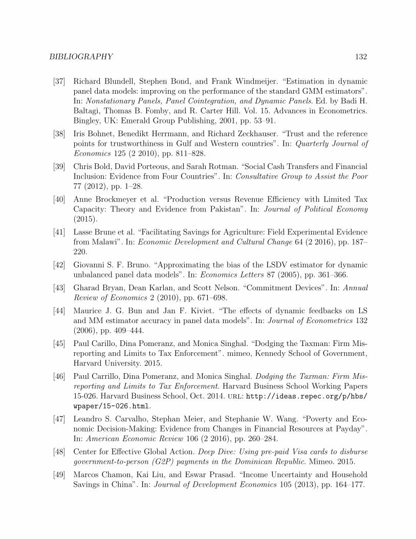
BIBLIOGRAPHY 132
[37] Richard Blundell, Stephen Bond, and Frank Windmeijer. “Estimation in dynamicpanel data models: improving on the performance of the standard GMM estimators”.In: Nonstationary Panels, Panel Cointegration, and Dynamic Panels. Ed. by Badi H.Baltagi, Thomas B. Fomby, and R. Carter Hill. Vol. 15. Advances in Econometrics.Bingley, UK: Emerald Group Publishing, 2001, pp. 53–91.
[38] Iris Bohnet, Benedikt Herrmann, and Richard Zeckhauser. “Trust and the referencepoints for trustworthiness in Gulf and Western countries”. In: Quarterly Journal ofEconomics 125 (2 2010), pp. 811–828.
[39] Chris Bold, David Porteous, and Sarah Rotman. “Social Cash Transfers and FinancialInclusion: Evidence from Four Countries”. In: Consultative Group to Assist the Poor77 (2012), pp. 1–28.
[40] Anne Brockmeyer et al. “Production versus Revenue E�ciency with Limited TaxCapacity: Theory and Evidence from Pakistan”. In: Journal of Political Economy(2015).
[41] Lasse Brune et al. “Facilitating Savings for Agriculture: Field Experimental Evidencefrom Malawi”. In: Economic Development and Cultural Change 64 (2 2016), pp. 187–220.
[42] Giovanni S. F. Bruno. “Approximating the bias of the LSDV estimator for dynamicunbalanced panel data models”. In: Economics Letters 87 (2005), pp. 361–366.
[43] Gharad Bryan, Dean Karlan, and Scott Nelson. “Commitment Devices”. In: AnnualReview of Economics 2 (2010), pp. 671–698.
[44] Maurice J. G. Bun and Jan F. Kiviet. “The e↵ects of dynamic feedbacks on LSand MM estimator accuracy in panel data models”. In: Journal of Econometrics 132(2006), pp. 409–444.
[45] Paul Carillo, Dina Pomeranz, and Monica Singhal. “Dodging the Taxman: Firm Mis-reporting and Limits to Tax Enforcement”. mimeo, Kennedy School of Government,Harvard University. 2015.
[46] Paul Carrillo, Dina Pomeranz, and Monica Singhal. Dodging the Taxman: Firm Mis-reporting and Limits to Tax Enforcement. Harvard Business School Working Papers15-026. Harvard Business School, Oct. 2014. url: http://ideas.repec.org/p/hbs/wpaper/15-026.html.
[47] Leandro S. Carvalho, Stephan Meier, and Stephanie W. Wang. “Poverty and Eco-nomic Decision-Making: Evidence from Changes in Financial Resources at Payday”.In: American Economic Review 106 (2 2016), pp. 260–284.
[48] Center for E↵ective Global Action. Deep Dive: Using pre-paid Visa cards to disbursegovernment-to-person (G2P) payments in the Dominican Republic. Mimeo. 2015.
[49] Marcos Chamon, Kai Liu, and Eswar Prasad. “Income Uncertainty and HouseholdSavings in China”. In: Journal of Development Economics 105 (2013), pp. 164–177.
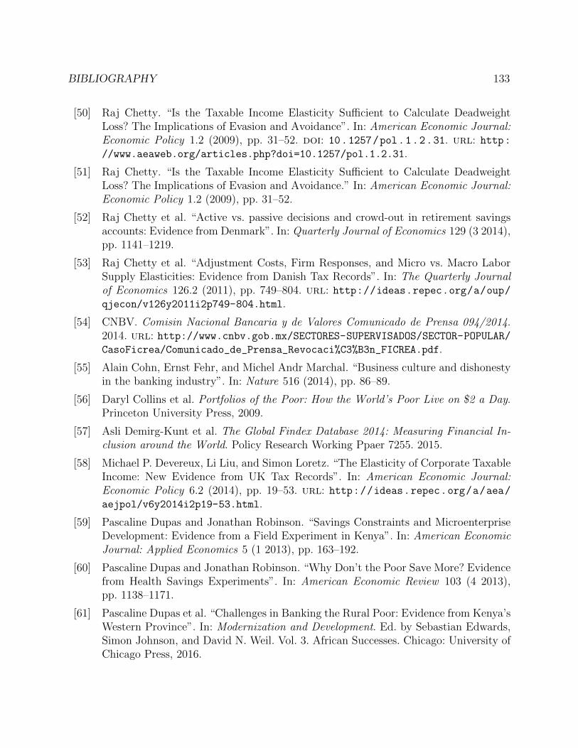
BIBLIOGRAPHY 133
[50] Raj Chetty. “Is the Taxable Income Elasticity Su�cient to Calculate DeadweightLoss? The Implications of Evasion and Avoidance”. In: American Economic Journal:Economic Policy 1.2 (2009), pp. 31–52. doi: 10.1257/pol.1.2.31. url: http://www.aeaweb.org/articles.php?doi=10.1257/pol.1.2.31.
[51] Raj Chetty. “Is the Taxable Income Elasticity Su�cient to Calculate DeadweightLoss? The Implications of Evasion and Avoidance.” In: American Economic Journal:Economic Policy 1.2 (2009), pp. 31–52.
[52] Raj Chetty et al. “Active vs. passive decisions and crowd-out in retirement savingsaccounts: Evidence from Denmark”. In: Quarterly Journal of Economics 129 (3 2014),pp. 1141–1219.
[53] Raj Chetty et al. “Adjustment Costs, Firm Responses, and Micro vs. Macro LaborSupply Elasticities: Evidence from Danish Tax Records”. In: The Quarterly Journalof Economics 126.2 (2011), pp. 749–804. url: http://ideas.repec.org/a/oup/qjecon/v126y2011i2p749-804.html.
[54] CNBV. Comisin Nacional Bancaria y de Valores Comunicado de Prensa 094/2014.2014. url: http://www.cnbv.gob.mx/SECTORES-SUPERVISADOS/SECTOR-POPULAR/CasoFicrea/Comunicado_de_Prensa_Revocaci%C3%B3n_FICREA.pdf.
[55] Alain Cohn, Ernst Fehr, and Michel Andr Marchal. “Business culture and dishonestyin the banking industry”. In: Nature 516 (2014), pp. 86–89.
[56] Daryl Collins et al. Portfolios of the Poor: How the World’s Poor Live on $2 a Day.Princeton University Press, 2009.
[57] Asli Demirg-Kunt et al. The Global Findex Database 2014: Measuring Financial In-clusion around the World. Policy Research Working Ppaer 7255. 2015.
[58] Michael P. Devereux, Li Liu, and Simon Loretz. “The Elasticity of Corporate TaxableIncome: New Evidence from UK Tax Records”. In: American Economic Journal:Economic Policy 6.2 (2014), pp. 19–53. url: http://ideas.repec.org/a/aea/aejpol/v6y2014i2p19-53.html.
[59] Pascaline Dupas and Jonathan Robinson. “Savings Constraints and MicroenterpriseDevelopment: Evidence from a Field Experiment in Kenya”. In: American EconomicJournal: Applied Economics 5 (1 2013), pp. 163–192.
[60] Pascaline Dupas and Jonathan Robinson. “Why Don’t the Poor Save More? Evidencefrom Health Savings Experiments”. In: American Economic Review 103 (4 2013),pp. 1138–1171.
[61] Pascaline Dupas et al. “Challenges in Banking the Rural Poor: Evidence from Kenya’sWestern Province”. In: Modernization and Development. Ed. by Sebastian Edwards,Simon Johnson, and David N. Weil. Vol. 3. African Successes. Chicago: University ofChicago Press, 2016.

BIBLIOGRAPHY 134
[62] Nadja Dwenger and Viktor Steiner. “Profit Taxation And The Elasticity Of TheCorporate Income Tax Base: Evidence From German Corporate Tax Return Data”.In: National Tax Journal 65.1 (2012), pp. 118–50. url: http://ideas.repec.org/a/ntj/journl/v65y2012i1p118-50.html.
[63] Karen E. Dynan, Jonathan Skinner, and Stephen P. Zeldes. “Do the Rich Save More?”In: Journal of Political Economy 112 (2 2004), pp. 397–444.
[64] Organisation for Economic Development and Co-Operation. “Tax Administration2013: Comparative Information on OECD and Other Advanced and Emerging Economies”.2013.
[65] M. Shahe Emran and Joseph E. Stiglitz. “On selective indirect tax reform in devel-oping countries”. In: Journal of Public Economics 89.4 (2005), pp. 599–623. url:https://ideas.repec.org/a/eee/pubeco/v89y2005i4p599-623.html.
[66] Diego Gambetta. Trust: Making and Breaking Cooperative Relations. Oxford: BasilBlackwell, 1988.
[67] Paul J. Gertler. “Do Conditional Cash Transfers Improve Child Health? Evidencefrom PROGRESA’s Control Randomized Experiment”. In: American Economic Re-view Papers and Proceedings 94 (2 2004), pp. 336–341.
[68] Paul J. Gertler, Sebastian W. Martinez, and Marta Rubio-Codina. “Investing CashTransfers to Raise Long-Term Living Standards”. In: American Economic Journal:Applied Economics 4 (1 2012), pp. 164–192.
[69] Roger Gordon and Wei Li. “Tax structures in developing countries: Many puzzles anda possible explanation”. In: Journal of Public Economics 93.7–8 (2009), pp. 855 –866.issn: 0047-2727. doi: http://dx.doi.org/10.1016/j.jpubeco.2009.04.001. url:http://www.sciencedirect.com/science/article/pii/S004727270900036X.
[70] Roger H. Gordon and Wei Li. “Tax Structures in Developing Countries: Many Puz-zles and a Possible Explanation”. In: Journal of Public Economics 2009.93 (2009),pp. 855–866.
[71] Yuriy Gorodnichenko, Jorge Martinez-Vazquez, and Klara Sabirianova Peter. “Mythand Reality of Flat Tax Reform: Micro Estimates of Tax Evasion Response and Wel-fare E↵ects in Russia.” In: Journal of Political Economy. 117.3 (2009).
[72] Jonathan Goyette. Optimal Tax Threshold: The Consequences on E�ciency of O�cialvs E↵ective Enforcement. Working Paper 12. 2012.
[73] Jonathan Gruber and Joshua Rauh. “How Elastic Is the Corporate Income Tax Base?”In: In Auerbach, Alan J., James R. Hines Jr., and Joel B. Slemrod (eds.), TaxingCorporate Income in the 21st Century Cambridge University Press (2007), pp. 140–163.
[74] Luigi Guiso, Paola Sapienza, and Luigi Zingales. “The Role of Social Capital in Fi-nancial Development”. In: American Economic Review 49 (3 2004), pp. 526–556.

BIBLIOGRAPHY 135
[75] Luigi Guiso, Paola Sapienza, and Luigi Zingales. “Trusting the Stock Market”. In:Journal of Finance 63 (6 2008), pp. 2557–2600.
[76] Jarkko Harju, Tuomas Kosonen, and Olli Ropponen. “Do Honest Hairdresses Get aHaircut? On Tax Rate and Tax Evasion”. mimeo, ZEW 2014 Public Finance Confer-ence. 2014.
[77] Albert O. Hirschman. “Against Parsimony: Three Easy Ways of Complicating SomeCategories of Economic Discourse”. In: American Economic Review Papers and Pro-ceedings 74 (2 1984), pp. 89–96.
[78] John Hoddinott and Emmanuel Skoufias. “The Impact of PROGRESA on Food Con-sumption”. In: Economic Development and Cultural Change 53.1 (2004), pp. 37–61.
[79] ILO. http://laborsta.ilo.org/informal economy E.html. 2012.
[80] IMF. “Medicion del Incumplimiento y del Gasto Tributario en Costa Rica”. In: (2012).
[81] Koichiro Ito and James M. Sallee. The Economics of Attribute-Based Regulation:Theory and Evidence from Fuel-Economy Standards. Working Paper 20500. NationalBureau of Economic Research, 2014. doi: 10.3386/w20500. url: http://www.nber.org/papers/w20500.
[82] Rajkamal Iyer and Manju Puri. “Understanding Bank Runs: The Importance ofDepositor-Bank Relationships and Networks”. In: American Economic Review 102(4 2012), pp. 1414–1445.
[83] William Jack, Adam Ray, and Tavneet Suri. “Money Management by Householdsand Firms in Kenya”. In: American Economic Review 103 (3 2013), pp. 356–361.
[84] William Jack and Tavneet Suri. “Risk Sharing and Transactions Costs: Evidence fromKenya’s Mobile Money Revolution”. In: American Economic Review 104 (1 2014),pp. 183–223.
[85] Matthew O Jackson and Leeat Yariv. “Present bias and collective dynamic choice inthe lab”. In: American Economic Review 104.12 (2014), pp. 4184–4204.
[86] Pamela Jakiela and Owen Ozier. “Does Africa Need a Rotten Kin Theorem? Experi-mental Evidence from Village Economies”. In: The Review of Economic Studies 83.1(2016), pp. 231–268.
[87] Alain de Janvry et al. “Delinking Land Rights from Land Use: Certification andMigration in Mexico”. In: American Economic Review 105 (10 2015), pp. 3125–3149.
[88] Dale Jorgenson and R.E. Hall. “Tax Policy and Investment Behavior”. In: AmericanEconomic Review 57 (1967). Reprinted in Bobbs-Merrill Reprint Series in Economics, Econ-130. Investment 2, ch. 1, pp 1-26., pp. 391–414.
[89] Steven N. Kaplan and Luigi Zingales. “Do Investment-Flow Sensitivities Provide Use-ful Measures of Financing Constraints?” In: The Quarterly Journal of Economics112.1 (1997), pp. 169–215.

BIBLIOGRAPHY 136
[90] Dean Karlan and Leigh L. Linden. Loose Knots: Strong versus Weak Commitmentsto Save for Education in Uganda? mimeo. 2014.
[91] Dean Karlan, Aishwarya Lakshmi Ratan, and Jonathan Zinman. “Savings by and forthe Poor: A Research Review and Agenda”. In: Review of Income and Wealth 60 (12014), pp. 36–78.
[92] Dean Karlan and Jonathan Zinman. Price and Control Elasticities of Demand forSavings. Working Paper. 2014. url: http://karlan.yale.edu/sites/default/files/savingselasticities_2014_01_v9.pdf.
[93] Dean Karlan et al. “Trust and social collateral”. In: Quarterly Journal of Economics124 (3 2009), pp. 1307–1361.
[94] Felipe Kast, Stephan Meier, and Dina Pomeranz. Under-savers anonymous: Evidenceon self-help groups and peer pressure as a savings commitment device. Harvard Busi-ness School Working Paper 12-060. 2012. url: http://www.hbs.edu/faculty/Publication%20Files/12-060_25eb4ab1-7f56-470b-b3a9-8e039b44118e.pdf.
[95] Felipe Kast and Dina Pomeranz. Saving More to Borrow Less: Experimental Evidencefrom Access to Formal Savings Accounts in Chile. Harvard Business School WorkingPaper 14-001. 2014. url: http://www.hbs.edu/faculty/Publication%20Files/14-001_2237a8d2-6147-4667-9396-cd5ae9702f03.pdf.
[96] Adnan Q. Khan, Asim I. Khwaja, and Benjamin A. Olken. “Tax Farming Redux:Experimental Evidence on Performance Pay for Tax Collectors”. In: The QuarterlyJournal of Economics (2015). doi: 10.1093/qje/qjv042. eprint: http://qje.oxfordjournals.org/content/early/2015/10/30/qje.qjv042.full.pdf+html.url: http : / / qje . oxfordjournals . org / content / early / 2015 / 10 / 30 / qje .qjv042.abstract.
[97] Jan F. Kiviet. “Expectations of expansions for estimators ina dynamic panel datamodel: Some results for weakly exogenous regressors”. In: Analysis of panels and lim-ited dependent variable models. Ed. by Cheng Hsiao et al. Cambridge, UK: CambridgeUniversity Press, 1999, pp. 199–225.
[98] Jan F. Kiviet. “On bias, inconsistency, and e�ciency of various estimators in dynamicpanel data models”. In: Journal of Econometrics 68 (1995), pp. 53–78.
[99] Henrik Kleven et al. “Unwilling or Unable to Chear: Evidence from a Tax AuditExperiment in Denmark”. In: Econometrica Vol. 79.No. 3 (2011), pp. 651–692.
[100] Henrik J. Kleven, Claus T. Kreiner, and Emmanuel Saez. “Why can Modern Gov-ernments Tax so Much? An Agency Model of Firms as Fiscal Intermediaries”. In:Economica (2016).
[101] Henrik J. Kleven and Mazhar Waseem. “Using Notches to Uncover OptimizationFrictions and Structural Elasticities: Theory and Evidence from Pakistan”. In: TheQuarterly Journal of Economics 128.2 (2013), pp. 669–723. url: http://ideas.repec.org/a/oup/qjecon/v128y2013i2p669-723.html.

BIBLIOGRAPHY 137
[102] Henrik Jacobsen Kleven. “How Can Scandinavians Tax So Much?” In: Journal ofEconomic Perspectives 28.4 (2014), pp. 77–98. doi: 10.1257/jep.28.4.77. url:http://www.aeaweb.org/articles.php?doi=10.1257/jep.28.4.77.
[103] Henrik Jacobsen Kleven et al. “Unwilling or Unable to Cheat? Evidence From a TaxAudit Experiment in Denmark”. In: Econometrica 79.3 (2011), pp. 651–692. issn:00129682. doi: 10.2307/41237767.
[104] Je↵rey R. Kling, Je↵rey B. Liebman, and Lawrence F. Katz. “Experimental Analysisof Neighborhood E↵ects”. In: Econometrica 75 (1 2007), pp. 83–119.
[105] Stephen Knack and Philip Keefer. “Does Social Capital Have an Economic Payo↵?A Cross-Country Investigation”. In: Quarterly Journal of Economics 112 (4 1997),pp. 1251–1288.
[106] Wojciech Kopczuk. “The Polish Business ”Flat” Tax and its E↵ect on ReportedIncomes: a Pareto Improving Tax Reform?” In: Working Paper, Columbia University(2012).
[107] Wojciech Kopczuk and Joel Slemrod. “Putting Firms into Optimal Tax Theory”. In:The American Economic Review: Papers and Proceedings 96.2 (2006), pp. 130–134.
[108] Todd J. Kumler, Eric A. Verhoogen, and Judith Frias. “Enlisting Workers in Monitor-ing Firms: Payroll Tax Compliance in Mexico”. mimeo, Columbia University. 2012.
[109] Rafael La Porta, Florencio Lopez de Silanes, and Guillermo Zamarripa. “RelatedLending”. In: Quarterly Journal of Economics 118 (1 2003), pp. 231–268.
[110] David Laibson. “Why Don’t Present-Biased Agents Make Commitments”. In: Quar-terly Journal of Economics 105 (5 2015), pp. 267–272.
[111] S. Levy and N. Schady. “Latin America’s social policy challenge: Education, socialinsurance, redistribution”. In: Journal of Economic Perspectives 27 (2013), pp. 193–218.
[112] Erzo F. P. Luttmer and Monica Singhal. “Culture, Context, and the Taste for Redis-tribution”. In: American Economic Journal: Economic Policy 3.1 (2011), pp. 157–79.url: https://ideas.repec.org/a/aea/aejpol/v3y2011i1p157-79.html.
[113] Erzo F. P. Luttmer and Monica Singhal. “Tax Morale”. In: Journal of EconomicPerspectives 28.4 (2014), pp. 149–68. url: https://ideas.repec.org/a/aea/jecper/v28y2014i4p149-68.html.
[114] John McMillan and Christopher Woodru↵. “Interfirm Relationships and InformalCredit in Vietnam”. In: Quarterly Journal of Economics 114 (4 1999), pp. 1285–1320.
[115] Suresh de Mel, Craig McIntosh, and Christopher Woodru↵. “Deposit collecting: Un-bundling the role of frequency, salience, and habit formation in generating savings”.In: American Economic Review Papers & Proceedings 103 (3 2013), pp. 387–392.

BIBLIOGRAPHY 138
[116] Bruce Meyer, Wallace K. C. Mok, and James X. Sullivan. “Household Surveys inCrisis”. In: Journal of Economic Perspectives 29 (4 2015), pp. 199–226.
[117] Sendhil Mullainathan and Eldar Shafir. “Savings Policy and Decision-Making in Low-Income Households”. In: Insu�cient Funds: Savings, Assets, Credit and BankingAmong Low-Income Households. New York City: Russell Sage Foundation Press, 2009,pp. 121–145.
[118] Fernando Naranjo and Guillermo Zuniga. “Manejo fiscal y deuda interna en CostaRica.” In: In: Gonzalez Vega, Claudio y Edna Camacho. Polıticas economicas enCosta Rica, Tomo I. Academia de Centroamerica: San Jose, Costa Rica (1990).
[119] Deepa Narayan and Lant Pritchett. “Cents and Sociability: Household Income andSocial Capital in Rural Tanzania”. In: Economic Development and Cultural Change(1999), pp. 871–898.
[120] Joanna Naritomi. “Consumers as Tax Auditors”. In: Working Paper, London Schoolof Economics (2015).
[121] Stephen Nickell. “Biases in Dynamic Models with Fixed E↵ects”. In: Econometrica49 (6 1981), pp. 1417–1426.
[122] Benjamin A. Olken and Monica Singhal. “Informal Taxation”. In: American EconomicJournal: Applied Economics 3.4 (2011), pp. 1–28. url: https://ideas.repec.org/a/aea/aejapp/v3y2011i4p1-28.html.
[123] Susan W. Parker and Graciela M. Teruel. “Randomization and Social Program Eval-uation: The Case of Progresa”. In: Annals of the American Acadamy of Political andSocial Science 599 (2005), pp. 199–219.
[124] Elena Patel, Nathan Seegert, and Matt Smith. “At a Loss: the Elasticity of CorporateIncome at the Zero Kink”. In: Working Paper (2015).
[125] Dina Pomeranz. “No Taxation without Information: Deterrence and Self-Enforcementin the Value Added Tax”. In: American Economic Review 8 (2015), pp. 2539–2569.issn: 0002-8282. doi: 10.1257/aer.20130393. url: http://qut.summon.serialssolutions.com/2.0.0/link/0/eLvHCXMwY2BQADaSjdJSU40tkpNTzZJNUlLTDBMNUo1TgLV9YmKqZRrKYBtSae4mxMCUmifKoOLmGuLsoQsrGuMTk0C9{\_}uSSYmA7FXQrMrDNb2woxsCbCFoDnlcC3iuWIsGgkGhungKqvyyBfQoTIxOzxCQTo8SktFRD40RgM9rEFADsbihJ.
[126] Dina Pomeranz. “No Taxation without Information: Deterrence and Self-Enforcementin the Value Added Tax”. In: American Economic Review 105.8 (2015), pp. 2539–69.doi: 10.1257/aer.20130393. url: http://www.aeaweb.org/articles.php?doi=10.1257/aer.20130393.
[127] Rafael La Porta et al. “Trust in Large Organizations”. In: American Economic As-sociation 87.2 (1997), pp. 333–338.
[128] Silvia Prina. “Banking the Poor via Savings Accounts: Evidence from a Field Exper-iment”. In: Journal of Development Economics 115 (2015), pp. 16–31.

BIBLIOGRAPHY 139
[129] Raghuram G. Rajan and Luigi Zingales. “Financial Dependence and Growth”. In:The American Economic Review 88.3 (1998), pp. 559–586.
[130] Risk-Based Tax Audits: Approaches and Country Experiences. Tech. rep. 2011.
[131] David Roodman. “A Note on the Theme of Too Many Instruments”. In: OxfordBulletin on Economics and Statistics 71 (1 2009), pp. 135–158.
[132] David Roodman. “How to do xtabond2: An introduction to di↵erence and systemGMM in Stata”. In: Stata Journal 9 (1 2009), pp. 86–136.
[133] Luis Rubalcava, Graciela Teruel, and Duncan Thomas. “Investments, time prefer-ences, and public transfers paid to women”. In: Economic Development and CulturalChange 57.3 (2009), p. 507.
[134] Emmanuel Saez. “Do Taxpayers Bunch at Kink Points?” In: American EconomicJournal: Economic Policy 2.3 (2010), pp. 180–212. doi: 10.1257/pol.2.3.180. url:http://www.aeaweb.org/articles.php?doi=10.1257/pol.2.3.180.
[135] Paola Sapienza and Luigi Zingales. “A Trust Crisis”. In: International Review ofFinance 12 (2 2012), pp. 123–131.
[136] Simone Schaner. “Do Opposites Detract? Intrahousehold preference heterogeneity andine�cient strategic savings”. In: American Economic Journal: Applied Economics 7(2 2015), pp. 135–174.
[137] Simone Schaner. “The Cost of Convenience? Transaction Costs, Bargaining, and Sav-ings Account Use in Kenya”. In: Journal of Human Resources (forthcoming).
[138] John Scott. “Redistributive Impact and E�ciency of Mexico’s Fiscal System”. In:Public Finance Review 42 (3 2014), pp. 368–390.
[139] Joel Slemrod, Marsha Blumenthal, and Charles Christian. “Taxpayer response to anincreased probability of audit: evidence from a controlled experiment in Minnesota”.In: Journal of Public Economics 79.3 (2001), pp. 455–483. url: https://ideas.repec.org/a/eee/pubeco/v79y2001i3p455-483.html.
[140] Joel Slemrod et al. Does Credit-card Information Reporting Improve Small-businessTax Compliance? NBER Working Papers 21412. National Bureau of Economic Re-search, Inc, July 2015. url: https://ideas.repec.org/p/nbr/nberwo/21412.html.
[141] Tavneet Suri, William Jack, and Thomas M. Stoker. “Documenting the Birth of aFinancial Economy”. In: Proceedings of the National Academy of Sciences 109 (262012), pp. 10257–10262.
[142] Jakob Svensson. “Who Must Pay Bribes and How Much? Evidence from a CrossSection of Firms”. In: Quarterly Journal of Economics 118.1 (2003), pp. 207–230.
[143] James Tobin. “The Interest-Elasticity of Transactions Demand for Cash”. In: Reviewof Economics and Statistics 38 (3 1956), pp. 241–247.

BIBLIOGRAPHY 140
[144] United Nations. “Report of the Intergovernmental Committee of Experts on Sustain-able Development Financing”. In: (2014).
[145] Oliver E. Williamson. “Calculativeness, Trust, and Economic Organization”. In: Jour-nal of Law and Economics 36 (1 1993), pp. 453–486.
[146] Frank Windmeijer. “A finite sample correction for the variance of linear e�cient two-step GMM estimators”. In: Journal of Econometrics 126 (2005), pp. 25–51.
[147] Philippe Wingender. “Tax Compliance and Financing”. mimeo, UC Berkeley. 2008.
[148] World Bank. “Financing for Development Post-2015”. In: (2013).
[149] Richard Wright et al. Less cash, less crime: Evidence from the Electronic BenefitTransfer program. NBER Working Paper 19996. 2014. url: http://www.nber.org/papers/w19996.
[150] James P. Ziliak. “E�cient Estimation With Panel Data When Instruments Are Prede-termined: An Empirical Comparison of Moment-Condition Estimators”. In: Journalof Business and Economic Statistics 15 (4 1997), pp. 419–431.
[151] Jonathan Zinman. “Credit or Debit?” In: Journal of Banking and Finance 33 (22009).