THE LONDON SCHOOL OF ECONOMICS AND POLITICAL

SCIENCE

Essays on the Causes of Migration

by

Daniel Richard Vernazza

A Thesis submitted to the Department of Economics of the London

School of Economics for the degree of Doctor of Philosophy

September 2012

Declaration

I certify that the thesis I have presented for examination for the PhD degree of the

London School of Economics and Political Science is solely my own work other

than where I have clearly indicated that it is the work of others (in which case

the extent of any work carried out jointly by me and any other person is clearly

identified in it).

The copyright of this thesis rests with the author. Quotation from it is permitted,

provided that full acknowledgement is made. This thesis may not be reproduced

without my prior written consent.

I warrant that this authorisation does not, to the best of my belief, infringe the

rights of any third party.

I declare that my thesis consists of 50,591 words.

1

AbstractThis thesis consists of three chapters. All three are linked by our desire to bet-

ter understand the determinants of labour migration; that is, the motivation fora person to change his or her location of residence for a period of at least a year.1

While immigration receives much public discourse, the economic evidence onhow migrants self-select is still lacking. In particular, we have little evidence onthe relative importance of determinants. We focus on three areas that have re-ceived substantially less attention in the migration literature: the importance ofrelative versus absolute income motives for migration; the effect of wealth andintertemporal choice on return migration; and the role of place attachment asan obstacle to labour mobility. Common to all three chapters is an emphasis oncounterbalancing forces that tend to offset spatial income differentials in deter-mining migration.

The first chapter examines the extent to which relative income – that is, one’sposition in the income distribution – matters in migration choice. Virtually allstudies of migration focus on absolute income. This is at odds with the mount-ing evidence that suggests people care about their relative position in the incomedistribution. We argue that, in order to test between the absolute income andrelative income theories of migration, one needs individual-level panel data onbefore and after migration outcomes. Indeed, since one has to estimate coun-terfactual migrant earnings of non-migrants, if migrants are selected on unob-servables then cross-sectional estimates will systematically bias the predictedmigrant earnings of non-migrants. We estimate the relative importance of thetwo main theories in explaining interstate migration in the U.S. using a panel ofindividuals. Relative income is calculated with respect to those persons in thesame U.S. state. We find that, although migration leads to a substantial rise inabsolute income, the trigger for migration is low relative income and not lowabsolute income.

In the second chapter we show analytically that, under some conditions, re-turn migration is optimal. We build a model where consumers choose eitherto never migrate, permanently migrate or, migrate and subsequently return. Togenerate an incentive for return migration, the model assumes a nominal incomedifferential between the source and destination and a compensating differential– which exerts a counterbalancing force to the income differential. Examples of

1This is consistent with the United Nation’s definition of a “long-term migrant” as “a personwho moves to a country other than that of his or her usual residence for a period of at least ayear”. Alternative definitions of a “migrant” based on birthplace or citizenship exist but are onlyuseful to the extent they are informative of where a person used to live, which is tenuous. Indeed,citizenship can change without moving and birthplace merely records residence at a single pointin time, birth, when the individual can do little to affect it!

2

compensating differentials may include differences between the source and des-tination in climate, place attachment, price levels, unemployment and averageconsumption. We characterise the optimal migration decision space with respectto the three key variables: initial wealth, the income differential and the compen-sating differential between the source and destination. The marginal utility ofconsumption is assumed to be location-dependent due to a non-separable non-pecuniary preference for the source. Consequently, when the region with thebest economic opportunities is not the source region, there is a trade-off betweenincome maximisation on the one hand and the marginal utility of consumptionon the other. We find that, all else equal, those with low wealth are more likely tomigrate and, conditional on migration, those with higher wealth are more likelyto return migrate.

The third chapter seeks to estimate a key obstacle to migration: place attach-ment. Place attachment refers to the emotional bonds a person feels towards theplace (or area) he or she resides. We estimate place attachment within a struc-tural model of spatial job search where migration is a by-product of accepting ajob offer from another region. The chapter can broadly be split into two parts.The first takes a standard job search model and adapts it to allow search in manypotential destinations. Acceptance of an offer from a destination necessarily in-volves migration to that destination and its associated costs. We consider twotypes of costs: a cost of migration that is related to distance-to-destination anda non-pecuniary cost of leaving the current region. The latter is deemed to bethe negative of place attachment. In the second part, we estimate the structuralmodel for a sample of individual durations in a U.S. state. Our estimates sug-gest that place attachment is steeply increasing in duration for our reduced-formmodel; however, the opposite is true for our structural model. We also find thatfor half the population, the dollar values of place attachment are prohibitivelylarge.

Thesis Supervisor: Silvana TenreyroTitle: Professor of Economics

3

Acknowledgements

The writing of this thesis has been the most frustrating, challenging and unfor-

gettable experience of my life. I would never have made it this far without the

support of my supervisor, colleagues, family and friends.

First of all, I want to thank Silvana Tenreyro, my supervisor, who has tirelessly

guided and encouraged me over many years. During my time as an LSE un-

dergraduate, masters student and now a doctoral candidate, Silvana has been

the most supportive and patient mentor. She inspired me to work on whatever

interests me, only asking that it be something of economic importance. I hope

I have achieved this. Without doubt all three chapters have improved substan-

tially as a result of her numerous comments and suggestions. Above all I thank

Silvana for believing in me.

Along the way I have been helped by numerous faculty members, classmates and

friends at the LSE. I have especially benefited from the comments of Francesco

Caselli, Javier Ortega, Yona Rubinstein and Thomas Sampson. I thank all the

participants at both the LSE Macro-money seminars and the CEP Labour Mar-

ket Workshop for their insightful comments. Over the years I have made many

friends at LSE; in particular I thank Abhimanyu Gupta, Aki Ishihara, Bonsoo

Koo, Michael McMahon, Prakarsh Singh and Kitjawat Tacharoen for the stimu-

lating discussions and all the laughs. All remaining errors are my own.

The biggest thank you goes to my family for their love and support. My mum

5

and dad are my inspiration and I dedicate this thesis to them. Without doubt I

would not have contemplated a PhD and I would not have made it this far with-

out their incredible support. They encouraged me to do well at school and to

reach for the sky. Any success I have in life is down to them. I also thank my

siblings, Matthew and Natalie, and my nan for their infinite encouragement.

I consider myself very fortunate to have a fantastic group of friends outside LSE

who have kept me (relatively) sane. Special thanks go to Jordan Jeewood, An-

drew Joyce and Robert Willis who stayed up late, spent a weekend and resched-

uled work, respectively, in order to read the thesis before submission. I benefited

from their comments and their effort and support will not be forgotten. I also

thank Chris Brown, John Hearn, Hannah Holland, Alexis Kiteos, Chanry Liu

and Szymon Ordys, among many others. Their friendship and support mean a

lot to me.

Finally, I thank the Economic and Social Research Council for their generous fi-

nancial support, without which I almost certainly would not have followed a

PhD but could have been a lot richer.

6

For my mum and dad

7

Contents

1 Does Absolute or Relative Income Motivate Migration? 13

1.1 Introduction . . . . . . . . . . . . . . . . . . . . . . . . . . . . . . . 13

1.2 Literature Review . . . . . . . . . . . . . . . . . . . . . . . . . . . . 21

1.2.1 Discussion . . . . . . . . . . . . . . . . . . . . . . . . . . . . 29

1.3 The Issue . . . . . . . . . . . . . . . . . . . . . . . . . . . . . . . . . 30

1.3.1 Absolute and Relative Income . . . . . . . . . . . . . . . . 34

1.3.2 Relative Deprivation . . . . . . . . . . . . . . . . . . . . . . 38

1.4 Empirics . . . . . . . . . . . . . . . . . . . . . . . . . . . . . . . . . 45

1.4.1 The Data . . . . . . . . . . . . . . . . . . . . . . . . . . . . . 46

1.4.2 Descriptive Statistics . . . . . . . . . . . . . . . . . . . . . . 52

1.4.3 Results . . . . . . . . . . . . . . . . . . . . . . . . . . . . . . 58

1.5 Concluding Remarks . . . . . . . . . . . . . . . . . . . . . . . . . . 90

Appendix 1.A Sample and Variable Construction for the Empirical Anal-ysis . . . . . . . . . . . . . . . . . . . . . . . . . . . . . . . . . . . . 101

2 Wealth, Intertemporal Choice and Return Migration 107

2.1 Introduction . . . . . . . . . . . . . . . . . . . . . . . . . . . . . . . 107

2.2 The Model . . . . . . . . . . . . . . . . . . . . . . . . . . . . . . . . 110

2.2.1 Location strategies . . . . . . . . . . . . . . . . . . . . . . . 112

2.2.2 Location decision rule . . . . . . . . . . . . . . . . . . . . . 117

2.3 Conclusion . . . . . . . . . . . . . . . . . . . . . . . . . . . . . . . . 122

Appendix 2.A Proofs . . . . . . . . . . . . . . . . . . . . . . . . . . . . 125

8

3 Place Attachment, Job Search and Migration: a Structural Estimation 130

3.1 Introduction . . . . . . . . . . . . . . . . . . . . . . . . . . . . . . . 130

3.2 The Model . . . . . . . . . . . . . . . . . . . . . . . . . . . . . . . . 138

3.2.1 The Migration Decision . . . . . . . . . . . . . . . . . . . . 141

3.2.2 The Choice Between Destinations . . . . . . . . . . . . . . 143

3.2.3 The Reservation Value . . . . . . . . . . . . . . . . . . . . . 146

3.2.4 The Conditional Migration Rate and Distribution of Dura-tion . . . . . . . . . . . . . . . . . . . . . . . . . . . . . . . . 147

3.3 Empirical Analysis . . . . . . . . . . . . . . . . . . . . . . . . . . . 148

3.3.1 The Data . . . . . . . . . . . . . . . . . . . . . . . . . . . . . 149

3.3.2 Descriptive Statistics . . . . . . . . . . . . . . . . . . . . . . 152

3.3.3 Empirical Model . . . . . . . . . . . . . . . . . . . . . . . . 160

3.3.4 Results . . . . . . . . . . . . . . . . . . . . . . . . . . . . . . 168

3.4 Conclusion . . . . . . . . . . . . . . . . . . . . . . . . . . . . . . . . 176

Appendix 3.A Data . . . . . . . . . . . . . . . . . . . . . . . . . . . . . 181

Appendix 3.B Fitting a Frechet distribution to the Empirical IncomeDistribution . . . . . . . . . . . . . . . . . . . . . . . . . . . . . . . 183

Appendix 3.C Matlab Code for the Structural Estimation . . . . . . . 186

9

List of Figures

2.1 Conditional value functions . . . . . . . . . . . . . . . . . . . . . . 120

2.2 Optimal location decision rule . . . . . . . . . . . . . . . . . . . . . 121

3.1 Density of a Frechet and Lognormal Distribution . . . . . . . . . . 145

3.2 Fitting a Lognormal to a Frechet: Maximum likelihood versus Kolmogorov-Smirnov distance minimisation . . . . . . . . . . . . . . . . . . . . 145

3.3 Interval Hazard Rate . . . . . . . . . . . . . . . . . . . . . . . . . . 159

3.4 Hazard rate for State Grew-up and Host Subgroups . . . . . . . . 159

3.5 Fitting a theoretical distribution to the empirical distribution ofwages and salaries in California and New York, 1990 . . . . . . . 185

3.6 Fitting a theoretical distribution to the empirical distribution ofpersonal income in California and New York, 1990 . . . . . . . . . 185

10

List of Tables

1.1 Descriptive Statistics: Means and Standard Deviations . . . . . . . 54

1.2 Distribution of Observations per Individual . . . . . . . . . . . . . 55

1.3 Distribution of Observations per Spell for Movers: Pre- and Post-Migration . . . . . . . . . . . . . . . . . . . . . . . . . . . . . . . . . 56

1.4 Distribution of the Number of Migrations per Individual . . . . . 57

1.5 Fixed Effects Estimates for Log Income, Relative Income and Rel-ative Deprivation for First-time Migrants . . . . . . . . . . . . . . 63

1.6 Fixed Effects Estimates for Log Income, Relative Income and Rel-ative Deprivation for All Migrants . . . . . . . . . . . . . . . . . . 66

1.7 Two Stage Least Squares Estimates . . . . . . . . . . . . . . . . . . 72

1.8 Pairwise Correlations . . . . . . . . . . . . . . . . . . . . . . . . . . 75

1.9 Average Partial Effects for Migration Propensity . . . . . . . . . . 80

1.10 Average Partial Effects for Migration Propensity: Controlling forRelative Deprivation . . . . . . . . . . . . . . . . . . . . . . . . . . 83

1.11 Robustness Checks . . . . . . . . . . . . . . . . . . . . . . . . . . . 85

3.1 Reason for Migration, by migration type, 1999-2011 . . . . . . . . 135

3.2 Distribution of Duration . . . . . . . . . . . . . . . . . . . . . . . . 156

3.3 Distribution of the Number of Spells per Individual . . . . . . . . 157

3.4 Distribution of Duration in subsample that drops left-censoredspells . . . . . . . . . . . . . . . . . . . . . . . . . . . . . . . . . . . 158

3.5 Maximum Likelihood Estimates of the Reduced-form Model . . . 170

3.6 Maximum Likelihood Estimates of the Reduced-form Model forsubsample that drops left-censored spells . . . . . . . . . . . . . . 173

11

3.7 Structural Maximum Likelihood Estimates for subsample that dropsleft-censored spells . . . . . . . . . . . . . . . . . . . . . . . . . . . 175

12

Chapter 1

Does Absolute or Relative

Income Motivate Migration?

“People care greatly about their relative income, and they would bewilling to accept a significant fall in living standards if they couldmove up compared with other people.”- Richard Layard (2005, p.43) “Happiness: Lessons from a New Science”

1.1 Introduction

Until recently, economists were in almost universal agreement that happiness

(or well-being) increased monotonically with income.1 Economic agents were

therefore defined by making choices – including migration – to maximise ex-

pected income. In the context of migration choice this implies that the higher

the income gain from migrating, the more likely migration occurs. It is no sur-

prise then that almost all models of migration assume the incentive to migrate

comes from the expected income differential between the source and destina-

1The mechanism is that higher income implies higher consumption – for given prices – and,in turn, greater happiness.

13

tion.2,3 Chief among these is Borjas’ (1987, 1991) model of income differentials,

which remains the most popular theory of migration twenty-five years after it

was published.4

However, there is a possible turning of the tide. Recent survey evidence

shows that happiness and life satisfaction are determined by relative income (to

others in some comparison group) as well as absolute income, and that once a

threshold level of income – needed for the essentials in life – is exceeded, hap-

piness no longer increases with absolute income but relative income instead.5

One way to change relative income is through migration.6 If relative income is

important, then we may observe situations that run counter to the absolute in-

come hypothesis. For example, if migration results in a deterioration in relative

income, people may choose not to migrate even when there is a potentially large

absolute income gain from doing so. Conversely – as the opening quote from

Layard (2005) suggests – people may migrate to improve their income position

even when the absolute income gain from migration is zero – or possibly, even

negative (a case often seen for return migrants).

The migration literature has been slow to catch-on. One visionary, Oded

Stark, did theorise that migration may depend on so-called relative deprivation be-

fore Borjas’ (1987) paper was published.7 Stark (1991) assumes people care about

2Throughout this chapter we use ‘source’ to denote the pre-migration location (or area) ofresidence and ‘destination’ refers to the post-migration location of residence. Therefore, migrationis the flow of people from the source to the destination.

3See, for example, the seminal works of Sjaastad (1962), Todaro (1969), Harris and Todaro(1970) and Borjas (1987, 1991).

4We refer to “absolute income” interchangeably with “Borjas” to describe the mechanism pro-posed by Borjas (1987, 1991).

5See, among others, Blanchflower and Oswald (2000), Frey and Stutzer (2002), Layard (2005)and Luttmer (2005). The idea that individuals care about relative income is not new: over sixtyyears ago Duesenberry (1949) argued that saving depends not on absolute income but on relativeincome.

6For example, migration will improve relative income when migration increases absolute in-come and the incomes of the comparison group are unchanged or, if migration involves no changein absolute income but a change in the comparison group to one on lower incomes.

7Stark (1984, 1991, 2006) and Stark and Yitzhaki (1988). See also Mehlum (2002) for how migra-tion is self-perpetuating (within and across generations) when relative deprivation is important.

14

their relative position in the income distribution (of some comparison group) and

that high relative deprivation increases the propensity of outmigration. More

specifically, Stark (1991) measures relative deprivation for an individual as the

fraction of people with higher incomes than that individual multiplied by their

average excess income.8,9

There is little or no empirical evidence to suggest which of these independently-

researched theories is the more important and, theoretically authors have either

not attempted to or not succeeded in distinguishing them. The purpose of this

chapter is therefore to analyse migration when both relative and absolute in-

come motives exist and, ultimately, to use panel data on interstate migration in

the United States to ascertain their relative importance in migration decisions.

Why is it important? If – and it’s a big if – relative income is found to be im-

portant and even dominate absolute income considerations in migration choice,

it will have profound implications. In summary, almost all existing economic

models of migration will be wrong, population forecasts will need to be recal-

culated and migration policy rethought. Indeed, the two theories can diverge

in their predictions. Firstly, under Stark’s relative deprivation theory, migrants

from the source region tend to be low-skilled (the deprived); whereas if the gain

in income from migration is greater for the high-skilled, then Borjas’ absolute

income theory tends to predict that migrants from the source are high-skill (a

brain drain). In section 1.3, we show formally that this divergence is due to

the asymmetric nature of Stark’s relative deprivation measure – it assumes peo-

ple compare themselves only with those on higher incomes (and not lower in-8We refer to “relative deprivation” interchangeably with “Stark” to refer to Stark’s mechanism.9The term relative deprivation originates from the social psychology literature. It refers to the

feeling of being deprived when comparing oneself to the better-off in one’s ‘reference group’.We feel this is a little unfortunate since deprivation typically conveys hardship and a lack of thenecessities in life. In contrast, by relative deprivation we mean the inverse of some measure ofrelative income or, more precisely, one’s position in the income distribution. Despite its slightlymisleading language, we stick with the term relative deprivation because it was used by Stark (1991)and, among others, it has been used in the study of income inequality and mortality (see, forexample, Deaton (2001)).

15

comes) than themselves. Second, a common concern of high-income regions is

that opening their borders to migrants from low-income regions will lead to a

flood of immigrants. To take one example, when Romania and Bulgaria joined

the European Union in 2007 many of the existing members introduced transi-

tional restrictions on immigration from these two countries.10 If, however, the

relative deprivation theory is correct, then the fears of high-income states may be

overstated; indeed, if migrants switch their reference group (with which income

comparisons are made) to the high-income destination, then they will likely find

that their relative deprivation worsens, which might make them more likely to

return-migrate.11 Finally, and we think most importantly, policy makers are not

only concerned with aggregate outcomes but individual outcomes too. In fact,

every vote counts. If the relative deprivation story is correct, then a transfer of

income from the rich to the poor is one way to improve the lives of the poor and

stem their outmigration; if however the absolute income story is correct then

the only way to improve the situation of the poor is to increase the income of

everyone.

While at first glance relative deprivation and absolute income motives may

appear easy to disentangle – after all they seem to speak to different moments of

the income distribution – the point is rather more subtle. Indeed, in aggregate

data, both Borjas and Stark can predict the ‘same’ relationship between income

inequality and the skill of migrants. More specifically, when income inequality

is higher in the source than the destination, both theories predict that migrants

will be of low-skill – for any given average income differential. The theories,

of course, differ in their underlying mechanism. In Borjas (1987, 1991) income

10Seventeen (out of twenty-five) EU member states restricted the free movement of labour fromRomania and Bulgaria when they joined the EU in 2007. Previously, transitional restrictions –which can last for up to seven years from the date of accession – were imposed on migrants fromthe 2004 EU accession countries, with the notable exceptions of Cyprus and Malta.

11Here the issue is whether there is a relative income motive for migration and, conditional ona relative income motive, whether one changes his or her reference group upon migration.

16

inequality reflects the return-to-skill, where a more unequal income distribution

implies a higher return-to-skill. Therefore when income inequality is higher in

the source than the destination, the return-to-skill is higher in the source and, it

is the low-skilled that are more likely to migrate from the source (for any given

average income differential).12,13 This confounds Stark’s relative deprivation the-

ory, which also predicts that the low-skilled (and, hence, low relative income) are

more likely to migrate from the source.

In section 1.3 we argue that the two theories can only be distinguished using

individual-level panel data on before and after migration outcomes. The reason

is that, with cross-sectional data, by definition one only observes income at a

single point in time, and for migrants this is typically after migration.14 In such

a case, one has to estimate the pre-migration income of migrants. However, if

migrants are selected on unobservables, then the estimated earnings of migrants

will be systematically biased. In contrast, with panel data we can directly com-

pute relative income prior to migration. Naturally, we will still want to estimate

the counterfactual earnings of non-migrants, but with panel data to hand we can

control for unobserved skill heterogeneity. In other words, we need panel data

to identify the high- and low-skilled.

The empirical literature on the determinants of migration has almost entirely

neglected to test for a relative income motive. Furthermore, the few papers that

do are systematically biased because they fail to control for the selection of mi-

grants on unobservables. To fill the void and test between the two theories, we

use panel data on individual interstate migration in the United States from the

Panel Study of Income Dynamics (PSID). We use the Current Population Survey

12The average income differential and the cost of migration affect the volume of migration butnot the selection-on-skill of migrants.

13These results require a certain degree of transferability of skills between the source and des-tination (see Borjas (1987)).

14A survey can only document migration if it has already occurred, whereas income is typicallyrecorded at the time of the survey.

17

(CPS) to estimate the distribution of income by state, from which we compute

relative deprivation for each individual-year in our PSID sample.

Since relative income is subjective, how researchers should measure it from

knowledge of the income distribution is open to debate. What is clear is that a

workable definition needs to be specific about two things. First, who constitutes

the group with which interpersonal comparisons are made? The evidence from

social psychology suggests that this reference group must be known to the indi-

vidual (that is, they know the income of the group members) and the person feels

that the income of the group members is a realistic expectation for himself. This

suggests geographical proximity and connectedness are important elements to

be considered. Naturally then, in the study of migration we will assume attach-

ment is to the people that reside within a geographical identifier, in our case a

U.S. state.15 That is, we assume the reference group for a person is the population

of the U.S. state that he or she resides in (or used to reside in).16

We will see that a pertinent question is whether, post-migration, a person

changes his or her reference group from the source to the destination; if so, then

we say reference substitution occurs. In Stark’s early papers (Stark, 1984, 1991,

Stark and Yitzhaki, 1988), the reference group was assumed to be the source ir-

respective of migration. From this viewpoint relative deprivation is a push fac-

tor since it is only the source income distribution that matters. Stark and Wang

(2000, 2005) were the first to acknowledge that individuals who care about rela-

tive income may in fact use migration in order to substitute their reference group

for another in the destination. From this viewpoint relative deprivation is both

15The geographical identifier for the reference group may well be much narrower than the statelevel. Luttmer (2005) finds that an increase in the earnings of those in the same U.S. Public UseMicrodata Area (PUMA) – which in 1990 had an average population of roughly 150,000 – reduceshappiness.

16Blanchflower and Oswald (2004) find that, for U.S. states, an increase in the average incomein the person’s state reduces that person’s happiness; however, if that person’s income rises in linewith the state average then that person gains overall.

18

a push and pull force for migration.17 Reference group substitution opens the

possibility that an individual may migrate to decrease relative deprivation (or

increase relative income) even if it involves no change in absolute income – or

possibly, even lowers income. We will consider the cases with and without ref-

erence group substitution.

The second thing that a definition of relative income must include is the func-

tional form for how one’s position in the income distribution equates to relative

income. Stark has proposed an ‘upward comparison’ view where an individual

compares his or her income with those people on higher incomes in the reference

group. More specifically, relative deprivation for person i is measured as the

product of the proportion of people with income higher than i and the mean ex-

cess income of these people (Stark, 1984, Stark and Yitzhaki, 1988). This is based

on evidence from social psychology that people look up and not down (see, for

example, Stouffer et al. (1949) and the references within Frey and Stutzer (2002)).

For completeness we also consider the symmetric case where individuals simply

compare their income to the average in the reference group.18

The empirical analysis in this chapter yields some novel results. First we

show that, using the sample of migrants, migration is associated with an in-

crease in absolute income and a reduction in relative deprivation. Therefore,

the extreme case that migrants move to lower their relative deprivation even

17Stark (2006) suggests that Borjas’ (1987) theory can be empirically distinguished from his ownrelative deprivation theory because Borjas (1987) emphasises income inequality in the destinationwhereas Stark’s theory pertains to income inequality in the source. However, this is not a gooddistinction, particularly if migration induces reference group substitution.

18Blanchflower and Oswald (2004) study the determinants of happiness in the U.S. and findevidence that individuals compare their income to the simple average income in the individual’sstate. More specifically, they also define relative income as the ratio of individual income to thestate average and they estimate its coefficient in a happiness regression to be positive and signif-icant, even after controlling for absolute income. The authors do, however, caution that relativeincome is not a complete explanation for the absence of increasing happiness in the U.S. over time.The authors also experiment with other measures of relative income, comparing individual in-come to quintile averages. They find tenuous evidence for the upward comparison view; morespecifically, the ratio of individual income to the top quintile performs better than the ratio withany other quintile.

19

when it involves a cut in absolute income is not supported in the data. However,

there is weak evidence that the observed percentage increase in relative income

post-migration is larger than would result purely from the observed percentage

increase in absolute income and no change in average income. By implication,

there is tentative evidence that migrants tend to target states where their position

in the income distribution improves holding absolute income constant.

Second, using the full sample of migrants and non-migrants, there is robust

evidence to support the relative deprivation hypothesis. We find that an increase

in relative deprivation increases the propensity to migrate from the source state.

Surprisingly, we find little or no evidence to support the absolute income the-

ory of migration that dominates the migration literature and the thinking of

policy makers. To be clear, although migrants tend to realise a rise in income

post-migration, our findings suggest that this is not the trigger for migration.

Rather our estimations suggest that – conditional on income and the estimated

income gain from migration – the trigger for migration is a rise in relative depri-

vation. These results hold after controlling for state-level compensating differen-

tials such as the price level, unemployment rate, and climate – as well as personal

characteristics such as age, education, marital status, number of children, home

ownership, and individual fixed effects.

Throughout the chapter we use the convention that migration – if it occurs –

is from the ‘source’ to the ‘destination’. Therefore, by definition, the source is the

pre-migration region and the destination is the post-migration region. Migrants,

outmigrants and immigrants all refer to people that have moved from the source

to the destination. Also, we use the term ‘positive selection’ to refer to the sit-

uation where migrants from the source have an average skill that exceeds the

average skill in the source. ‘Negative selection’ is used to describe the situation

where the average skill of migrants is below the average skill in the source.

20

The rest of the chapter is organised as follows. Section 1.2 discusses the re-

lated literature. In section 1.3 we formally identify the problems with distin-

guishing Borjas’ absolute income model from Stark’s relative deprivation model

of migration. Section 1.4 contains a description of the data, the empirical strategy

and the estimation results. Finally, section 1.5 concludes.

1.2 Literature Review

Since a major contribution of this chapter is to highlight the current literature’s

failure to estimate the effect of relative income on migration, it seems appropriate

to dedicate a whole section to reviewing the related literature. Our work is re-

lated to four distinct literatures. In decreasing order of importance (for our work)

they are: (1) a handful of papers that claim to jointly estimate the importance of

relative and absolute income motives for migration; (2) papers that proclaim to

test empirically the selection predictions of Borjas’ model; (3) papers that show

relative income affects utility and can help to explain a number of (not migration

related) economic puzzles and, (4) papers that show migrants respond to abso-

lute income differentials (without controlling for relative income considerations).

We take each of these in turn.

Stark and Taylor (1989, 1991) find that, after controlling for the expected ab-

solute income gain, relatively deprived Mexican households were more likely to

migrate to the United States. However, in section 1.3 we show that if migrants

are positively selected on unobservables, then their result is biased in favour

of the finding that relative deprivation matters. The problem is that they use

cross-sectional data, which precludes controlling for selection on unobservables

when they estimate counterfactual income of migrants and non-migrants from

the earnings of non-migrants and migrants, respectively. Quinn (2006) studies

21

the effect of relative deprivation (and not just in terms of income but wealth too)

on the migration of Mexican households. However, this suffers from the same

problem as Stark and Taylor (1989, 1991) because it is cross-sectional.

In a working paper, Basarir (2012) uses panel data on internal migration in

Indonesia to study absolute and relative motives for migration.19 The empirical

analysis uses the final two waves of data, 2000 and 2007, of the Indonesian Fam-

ily Life Survey. The author estimates the effect of absolute and relative measures

of expenditure, income and assets on the propensity to migrate. He finds that

men are more likely to migrate if they expect to improve their expenditure rank,

even if it involves a loss in absolute expenditure. The future ranking of income

and assets is statistically insignificant. The author finds that initial absolute ex-

penditure is negatively related to the propensity to migrate; whereas the effects

of initial income and assets are insignificant. There is no evidence to suggest that

a low initial rank increases migration propensity holding absolute measures con-

stant. Basarir (2012) is similar to our work in both its aims and its use of panel

data; however, there are some key differences. The dependent variable in Basarir

(2012) is a dummy variable for whether the individual moved out of the source

sub-district for a period of more than six months between 2000 and 2007, so there

is no precise information on the timing of migration, nor can the author identify

return migrants. In contrast, our PSID data follows individuals annually (or bi-

ennially) and so we can pin-point the timing of migration and ascertain whether

the individual is returning to a state he or she previously resided. In particu-

lar, we can relate the migration decision to the socio-economic characteristics of

the individual at the time of migration. Also, Basarir (2012) uses actual future

values of expenditure, income and assets to proxy for the expected gain from

migration. Such an approach introduces endogeneity concerns. Instead, using

our long-running PSID panel dataset, we estimate the contemporaneous coun-

19We only became aware of Basarir (2012) after completion of this chapter.

22

terfactual (migrant) income of non-migrants, whilst controlling for unobserved

heterogeneity. Still, Basarir (2012) can be considered complementary to our work

since it studies migration within a developing country, Indonesia, whereas our

data is for the U.S..

A number of papers have sought to test Borjas’ selection theory. Unfortu-

nately, none of these are a test between Stark’s and Borjas’ theory. Moreover,

where evidence has been found in favour of Borjas’ theory (and, on the whole,

the evidence is mixed) it equally can serve as evidence for the relative income

story.20 Early work on this looked at variation in the earnings of U.S. immi-

grants with the same observable skills and related this to income inequality in

their source countries.21 Borjas (1987) uses U.S. Census data from 1970 and 1980

and compares the earnings of U.S. immigrants from 41 countries with income in-

equality (measured as the ratio of the top 10 percent to the bottom 20 percent) in

the source. He finds weak evidence in support of his selection theory: income in-

equality in the source has a small negative impact on immigrant quality.22 Ramos

(1992) finds that U.S. immigrants from Puerto Rico are on average less educated

than Puerto Ricans who remained in Puerto Rico. Further, those U.S. immigrants

who subsequently returned to Puerto Rico were more educated than the pool of

migrants that did not return. Since the return-to-skill in Puerto Rico was higher

than that on the U.S. mainland, this result is consistent with Borjas’ selection the-

ory. Nonetheless, we argue that the findings of Ramos (1992) are also consistent

20The vast majority of papers that seek to test Borjas’ selection predictions study Mexico-to-U.S. migration. Since income inequality is higher in Mexico than the U.S., Borjas’ model predictsnegative selection of migrants. Of course, low-skilled migrants also tend to be relatively deprived.

21See Borjas (1994, pp. 1690) for a summary. Later we will argue that, to test between the relativeand absolute income stories, it is necessary to use individual-level data. Since many of thesestudies use country-level migration data, this confounds absolute and relative income motives formigration.

22The negative effect of source income inequality on U.S. immigrant quality vanishes whenincome per capita in the source is controlled for. Borjas suggests this is due to the high negativecorrelation between income inequality and income per capita across countries. Using the changein the percentage of GNP that is spent by government in the source as a proxy for the change inincome inequality over time, Borjas finds that this measure is positively correlated with the changein immigrant quality, which is consistent with his selection theory.

23

with the relative deprivation theory since the less educated tend to be the more

relatively deprived.

The more recent evidence on Borjas’ selection theory is mixed. Liebig and

Sousa-Poza (2004) look at the intention to migrate using data from the 1995 Inter-

national Social Survey Programme for a cross-section of 23 countries.23 Again,

their dataset is cross-sectional so they cannot control for selection-on-unobservables.

Nonetheless, the survey asks whether the respondent is willing to move to an-

other country to better work or living conditions. They correlate this with mea-

sures of income inequality (including the Gini coefficient) in the source country,

while controlling for other individual socio-demographic characteristics. They

find that higher income inequality in the source is correlated with a higher ag-

gregate propensity to migrate even after controlling for the level of income. Stark

(2006) interprets this finding of Liebig and Sousa-Poza as evidence in favour of

relative deprivation and shows algebraically that his measure of relative depri-

vation is positively related to the Gini coefficient. Interestingly, however, Liebig

and Sousa-Poza (2004) find that the positive effect of education on migration is

much larger than the negative effect of income inequality and so conclude that

migrants are typically positively selected (on education) irrespective of income

inequality. In other words, higher income inequality reduces the positive selec-

tion of migrants, but it remains positive. This is not what Borjas (1987) or Stark

predicts; it is however consistent with Borjas (1991) in which he extends his ear-

lier (1987) theory to allow for selection on observables (such as education) as

well as selection on unobservables. Indeed, Borjas (1991) shows that – assum-

ing observable education is uncorrelated with the unobservables – it is possible

to have positive selection on education and negative selection on unobservables

23The authors argue that, by studying the intention to migrate, they reduce the difficulties withidentifying selection that occur when using host country data on migrants from different sourcecountries. In particular, the skills of immigrants are likely to be highly distorted by (skill-biased)immigration policy and migration networks. In our empirical analysis, immigration policy is notan issue since we study interstate migration.

24

(or vice versa). This would occur if the return to education is higher in the des-

tination than the source and yet, income inequality within the group of persons

with the same observed education is higher in the source than the destination.

Whilst theoretically possible, we would expect (and hope) that education and

unobserved ability are positively correlated. Therefore, Liebig and Sousa-Poza

(2004) (who make no mention of relative deprivation) suggest it is evidence in

favour of Chiswick (1999), which can be viewed as an extension of Borjas (1987)

to a situation where time-equivalent migration costs are decreasing with ability

and predicts positive selection of migrants.24

More specifically, Chiswick (1999) hypothesizes that migration costs have

a shorter time-equivalent for high-ability (and therefore high-income) workers

compared to low-ability (and low-income) workers.25 Consequently, migrants

are positively selected from the source skill distribution. In contrast, Borjas (1987)

assumes the time-equivalent moving cost is identical for all skill types (that is,

the cost of migration is proportional to the source wage). In summary, Chiswick

(1999) predicts that, although Borjas’ mechanism is still valid, it is not enough

to overturn the positive selection; hence Borjas’ mechanism (that higher source

income inequality implies negative selection from the source) merely leads to

‘less favourable selectivity’ but, importantly it is still positive.26 Chiquiar and

Hanson (2005) use the 1990 and 2000 Mexican and U.S. Censuses and find that,

24More recent theoretical contributions include Clark et al. (2007) who extend the Borjas modelto account for non-pecuniary benefits and various costs of migration but do not consider relativeincome (or relative deprivation) motives.

25This can be achieved in a number of ways. Chiswick (1999) first assumes that out-of-pocketcosts are independent of individual ability such that time-equivalent migration costs are lower forhigher ability workers (that is, the same cost is scaled by a higher wage for higher ability workers).Alternatively, as Chiswick (1999) says, if high-ability workers are more efficient at moving thenthey have lower absolute out-of-pocket migration costs and, additionally, may spend less timeon migration thereby reducing foregone earnings (therefore, forgone earnings are not a constantproportion of earnings across abilities).

26There is some evidence that after some initial downgrading of earnings for new immigrants,eventually the earnings of the foreign-born outperform those of natives, even after controlling forobservable characteristics such as education (see Chiswick (1978, 1986a,b) for the U.S. and Bloomand Gunderson (1991) for Canada). This suggests positive selection of migrants, although Borjas(1985) questions the overtaking for the U.S..

25

rather than Mexican migrants being selected from the left tail of the (more un-

equal) skill distribution in Mexico (as Borjas’ theory would suggest), they tend

to come from the middle. The authors propose that this is consistent with Borjas’

theory if the costs of migration fall with education, as hypothesised by Chiswick

(1999). In recent work, Ambrosini and Peri (2011) find support for Borjas’ theory

from individual-level panel data on Mexico-U.S. migration. They control for se-

lection on observables and unobservables and find that on average there is neg-

ative selection of U.S. immigrants from Mexico. This is consistent with Borjas’

story because income inequality is higher in Mexico than the U.S.. Importantly,

they find that almost all of the negative selection is on unobservable character-

istics, which they claim is why cross-sectional studies of Mexico-U.S. migration

(such as Chiquiar and Hanson (2005)) do not find negative selection. In terms

of how this differs from our work, the authors do not consider relative income

(or relative deprivation) as an explanatory variable for migration and, therefore,

cannot distinguish between Borjas and Stark. Indeed, given that income is more

unequal in Mexico than the U.S., evidence of negative selection is consistent with

both Borjas and Stark’s story – the low-skilled tend to be the relatively deprived..

The notion that relative income – in addition to absolute income – may drive

migration choice is persuasive given the recent evidence that subjective well-

being (or happiness) is increasing in relative income as well as absolute income.

There exist a number of country-level surveys that ask people to rate how happy

they feel on a scale, for example, from 1 to 10. In a series of papers Richard East-

erlin found that, whilst rich people are happier than poor people within the same

country, across countries those in rich countries were on average no happier than

those in poor countries (Easterlin, 1974, 1995, 2001).27 This became known as the

Easterlin paradox. Further, while at any point in time the rich are markedly

happier than the poor within a country, over time as per capita incomes have

27A notable exception is the very poor countries who are less happy.

26

increased there has been no discernible change in happiness (see, for example,

Frey and Stutzer (2002) and Layard (2005)). A common explanation advanced

by Easterlin and others is that happiness depends on relative income; that is, a

person compares his income to the incomes of those in the same country or lo-

cality. Moreover, above a threshold income needed to buy the essentials in life,

happiness seems to be determined solely by relative income.28

Luttmer (2005) uses the U.S. National Survey of Families and Households to

study the relationship between individual well-being (measured by self-reported

happiness) and average income in the Public Use Microdata Area (PUMA) that

the individual inhabits. Luttmer finds that, controlling for own household in-

come, an increase in PUMA average earnings reduces reported happiness. Im-

portantly, the result holds after controlling for individual fixed effects. Also,

while the coefficient estimate on own household income is positive and larger

(in absolute value) than the coefficient estimate on PUMA average earnings, they

are not statistically different from each other; hence, Luttmer cannot reject the

hypothesis that only relative income matters.

However, the relative income hypothesis has been heavily disputed by Deaton

(2008) and Stevenson and Wolfers (2008). They find that rich countries are hap-

pier than poor countries and, the ratio is roughly the same as that between rich

people and poor people within the same country. Moreover, Stevenson and

Wolfers (2008) find no evidence of a satiation point for happiness as income

grows – only absolute income matters. In response, Layard et al. (2010) argue

that Deaton (2008) and Stevenson and Wolfers (2008) are mainly cross-sectional

in nature and so it is unclear whether income is proxying for unobservables. Fo-

cussing on developed countries, Layard et al. (2010) find that – within-countries

28The idea that relative income – and, in particular, relative deprivation – matters for well-beinghas been met with increasing acceptance in social psychology. The term relative deprivation wasfirst coined by Stouffer et al. (1949) to explain why army personnel satisfaction increased witharmy rank.

27

and over time – there is a positive link between relative income and happiness.

In the U.S., average happiness has not risen since the 1950s and this is at a time

when average income has increased dramatically. Stevenson and Wolfers (2008)

admit that this is something of a puzzle. Easterlin et al. (2010) look at a large

sample of both developed and developing countries and find that over time hap-

piness does not increase with a country’s income.

A very much related literature is that which uses external habits (that is,

keeping-up or catching-up with the Joneses) to explain a broad range of anoma-

lies in economics (Clark et al., 2008), including mortality (Wilkinson, 1996). The-

oretically, relative income can also provide an explanation for the phenomenon

that is return migration (Stark, 1991). Return migration – the process of returning

to a region once resident in – represents a large percentage of two-way migration

flows (see, for example, Eldridge (1965) for U.S. interstate migration). A lower

average income in the source than the host region may provide an incentive to

return to the source if individuals care about their position in the income distri-

bution.

Finally and more generally, this chapter is related to the large empirical litera-

ture on the determinants of migration. A vast number of papers (far too many to

mention) have found that absolute income differentials influence migration (see

Greenwood (1975, 1985) for surveys on the determinants of internal migration).

These papers do not control for relative income. In our empirical analysis we will

want to control for those variables that explain migration and are potentially cor-

related with individual income and average income in a region. Potential con-

founding factors are regional compensating differentials that act as a counterbal-

ancing force to the income differential between the source and destination. Ex-

amples of compensating differentials mentioned in the literature are differentials

in the unemployment rate (Todaro, 1969, Harris and Todaro, 1970); prices (Djajic,

28

1989, Dustmann, 1995, 2003, Stark et al., 1997, Dustmann and Weiss, 2007); and

climate (Graves, 1980) between the source and destination. In our estimations

of the propensity for interstate migration, we control for these at the state level.

In addition, we control for a number of personal characteristics that have been

found to influence migration.

1.2.1 Discussion

There is a related and interesting side order. Given the large, persistent differ-

ences in per capita income that exist across countries and regions, a migration

theory based on income maximisation alone would seem to predict much larger

migration flows than we actually observe. To reconcile this, the advocates of

income maximisation have offered three explanations. The first is that interna-

tional migration is highly regulated and so there are people that want to move

but do not meet the criteria for legal entry. Whilst certainly part of the story, it is

clearly not a full explanation because there are many counterexamples. Indeed,

where migration is unregulated (such as within the European Union and region-

ally), big differences in per capita incomes exist yet only a small portion of the

population migrate.29 Second, the absolute income camp would argue that un-

employment (or the probability of finding a job) is the counter-balancing force

(Todaro, 1969, Harris and Todaro, 1970).30 However, there is little evidence to

support the Harris-Todaro prediction of compensating unemployment differen-

29Eurostat figures for 2010 show that just 3.2 percent of European Union residents were born ina different member state to the one they currently reside in.

30Todaro (1969) presents a model of rural-urban migration in less-developed countries basedon the expected wage differential – that is, the product of the urban-rural earnings differential andthe probability of being employed. In Todaro (1969), increased rural-to-urban migration reducesthe expected urban wage because it reduces the probability of employment. Accounting for theprobability of unemployment can simultaneously explain two phenomena: persistent wage dif-ferentials across regions (unemployment is the clearing mechanism in the presence of urban wagerigidities) and yet continued migration to urban areas facing unemployment. Although Todaro’smodel is targeted at explaining rural-urban migration in LDCs, it has relevance for regional andinternational migration. Furthermore, Todaro’s mechanism moves towards a general equilibriumframework since migration affects the probability of employment.

29

tials for wage differentials, at least among the less educated (see, for example,

Fields (1982) for Colombia and Schultz (1982) for Venezuela). The implication is

that expected income differentials across regions exist. Indeed, as Raimon (1962)

finds, the U.S. states with above average earnings tend to have above average

employment increases. Third – and we think the most convincing response –

is that the costs of migration (monetary and psychic) are very high. Since the

monetary (one-off) costs of moving would have to be implausibly high, it ap-

pears non-pecuniary (or psychic) costs are large. It is, however, not satisfactory

to have no theory to explain (endogenise) these non-pecuniary costs. There are a

couple of candidates; place attachment is the obvious one but another is relative

income (or relative deprivation).

1.3 The Issue

In this section, we will show that – under some conditions – all three theories

(absolute income, relative income and relative deprivation) predict the same ag-

gregate relationship between (1) income inequality and the selection of migrants

and, (2) income inequality and the outmigration rate from the source. To be clear,

there is no general result here; we simply show that under some conditions the

three theories lead to the same predictions. Indeed, a simple counterexample is

all we need to refute the claims of those that purport empirical evidence on mi-

grant selection to prove or disprove any one theory. To show this we take Borjas’

(1987) absolute income model of migration and extend it to include a relative

income and a relative deprivation motive for migration.31

We make three assumptions: (A1) the distribution of skill (or ability) in the

source is Normally distributed; (A2) the ordinal ranking of individuals in the

31Borjas (1987) formalises the Roy (1951) model of self-selection into different occupations andapplies it to migration.

30

source does not change if moved to the destination (that is, if we moved the

whole population of the source to the destination, the ordinal ranking of these

individuals in the destination income distribution is unchanged from that in the

source income distribution); (A3) migration is modelled as a one-shot decision

(static model), there are no strategic interactions between individuals and no

feedback effects of migration on income.32 Regarding assumption A3, it will

help to think of our model as an experiment where we consider simultaneously

moving everyone in the source to the destination and we ask who in the source

is likely to agree to this. The simultaneous movement of everyone allows us to

ignore general equilibrium effects of migration.33 One could get different results

from changing one or more of these assumptions. We make such stark assump-

tions for the sake of clarity and exposition, but these assumptions are relaxed

later in the empirical analysis.

In what follows we use a subscript 0 to denote the source and a subscript 1 to

denote the destination. Log income in the source is assumed to be

log y0 = µ0 + ηε, (1.1)

where µ0 is average income in the source, ε is skill (or ability) and, η ≥ 0 is

the return to skill in the source. We assume skill is unobservable; however, we

know that skill in the source population is independent, standard Normally dis-

tributed: ε ∼ N (0, 1). Let Y0 denote the random variable for income in the

source, it is Log-normally distributed: Y0 ∼ Log-N (µ0, η2).

32Borjas (1987) assumes (A1) and (A3); among others, Borjas and Bratsberg (1996) assumes (A2).These assumptions are more restrictive than we actually need; for example, the (ordinal) rankingof skills in the destination and source need not be identical – our results would go through if thecorrelation between the income distribution of the source and destination is sufficiently high (seeBorjas (1987)). These assumptions are not used in the empirical analysis of Section 1.4.

33If interaction or feedback effects of migration occur, then the migration decision of a personwill depend on the migration choice of others. For example, immigration will increase labour sup-ply in the destination and this may lower the wage. Also, migration will change the distributionof income for those left behind and this may affect their decision to migrate if individual utilitydepends on the incomes of others (see Stark (1984)).

31

If all those in the source migrate to the destination, log earnings in the desti-

nation is assumed to be

log y1 = µ1 + ε, (1.2)

where µ1 is average income that migrants receive in the destination if all per-

sons from the source migrate to the destination. Notice we have normalised

the return to skill in the destination to unity so that η is now the return to skill

in the source relative to that in the destination.34 The relative return to skill in

the source, η, is implicitly the outcome of differences in endowments and re-

distributional policy between the source and destination. The random variable

for income (of the source population) in the destination is Log-normally dis-

tributed: Y1 ∼ Log-N (µ1, 1). For expositional purposes, in what follows we

will assume that average income is higher in the destination than the source:

E(Y1) > E(Y0), ∀η and µ1 > µ0.35

A definition of relative income and relative deprivation needs to be specific

about who constitutes the ‘reference group’ to which income comparisons are

made. We assume the reference group is the population of the source; however,

whether we use their source incomes or their (potential) destination incomes will

depend on whether we assume ‘reference substitution’ occurs post-migration.

For a non-migrant, his or her reference is assumed to be the source income distri-

bution; for a migrant his or her reference remains the source income distribution

except when we assume reference substitution takes place, in which case the

34We have used our assumption of constant rank here; that is, the distribution of skills in thesource is the same as that in the destination. This assumption rules out movement within theskill distribution upon migration – the ordinality (or ranking) of skills is the same in both regions.Borjas’ (1987) paper allows for variable correlation (ρ) between the skill distribution of the tworegions. Borjas characterises selection conditional on ρ as well as the relative return to skill η. Ourmodel is the special case of Borjas where ρ = 1, which is reasonable for U.S. interstate migrationsince the transferability of skills across states is high.

35E(Y1) = exp(µ1 + 0.5) and E(Y0) = exp(µ0 + 0.5η2). Therefore, for E(Y1) > E(Y0) we requireµ1 − µ0 > 0.5(η2 − 1).

32

reference switches to the destination income distribution. Let FYj(y) denote the

(Log-normal) cumulative distribution function of income in reference j. Then,

for an individual with income y and reference j, we define his or her absolute

income (AI(y)), relative income (RI(y, j)) and relative deprivation (RD(y, j)) as

AI(y) ≡ y; (1.3)

RI(y, j) ≡ yE(Yj)

; (1.4)

RD(y, j) ≡∫ ∞

y(x− y)dFYj(x) (1.5)

= [1− FYj(y)][E(Yj|Yj > y)− y] (1.6)

=∫ ∞

y[1− FYj(x)]dx. (1.7)

That is, relative income (RI(y, j)) is the ratio of individual income to average in-

come in the reference group. The symmetric nature of relative income means

that a greater sense of happiness (unhappiness) is felt when income is further

above (below) the mean. Our measure of relative deprivation in equation (1.5)

is identical to that proposed by Stark (1991). Relative deprivation of a person

with income y and reference j, RD(y, j), is the sum of the excess income above

y over all those people in j with higher incomes than y. Equation (1.6) follows

directly from expanding the integral in (1.5). It says that RD(y, j) equals the pro-

portion of people in j with higher incomes than y weighted by their mean excess

income over y.36 Equation (1.7) results from integration by parts of equation (1.5)

(Yitzhaki, 1979).37 Note a difference between relative deprivation and relative in-

come as we have defined it above is that relative deprivation is not symmetric:

everyone is deprived apart from the top person who feels nothing. This will af-

fect the results.38 In the remainder of this section, we first solve the model with a36∫ ∞

y (x− y)dFYj (x) =∫ ∞

y xdFYj (x)− y∫ ∞

y dFYj (x) = E(Yj|Yj > y)[1− FYj (y)]− y[1− FYj (y)].

37∫ ∞y (x− y)dFYj (x) = (x− y)FYj (x)

∣∣∣∣∞y−∫ ∞

y FYj (x)dx =∫ ∞

y [1− FYj (x)]dx.

38Although in Stark’s measurement of relative deprivation only those with higher incomes are

33

utility function that nests the absolute income and relative income motives. The

model with relative deprivation is deferred to subsection 1.3.2.

1.3.1 Absolute and Relative Income

Assume individual utility depends on both absolute income and relative income.

Specifically, the indirect utility of a person with income y is assumed to be

U(y, j) =y[

E(Yj)]δ

,

where δ ∈ [0, 1] is the weight attached to relative income in utility. Clearly, if

δ = 0 then U(y, j) = AI(y) and, if δ = 1 then U(y, j) = RI(y, j).

First consider the case where post-migration the reference remains the source

income distribution (that is, no reference substitution takes place). Then migra-

tion is optimal if

y1

[E(Y0)]δ>

y0 + C

[E(Y0)]δ,

where C ≥ 0 is the cost of migration. After taking logs we have

log y1 > log y0 + log(

1 +Cy0

),

which does not depend on δ. We follow Borjas (1987) and assume the time-

equivalent cost of migration π ≡ Cy0

is constant. This implies that the cost of

migration is proportional to income in the source. Then the condition for migra-

included in the calculation, those on lower incomes affect the calculation via their effect on theweights.

34

tion is approximately39

(1− η)ε > − (µ1 − µ0 − π) , (1.8)

and the probability of migration is

Pr(Migrate) = 1−Φ(zNRS);

where zNRS =− (µ1 − µ0 − π)

|1− η| , (1.9)

where Φ denotes the distribution function of the standard Normal and the su-

perscript NRS stands for No Reference Substitution. The selection of migrants

from the source income distribution is given by the average income in the source

conditional on migration

E(log y0|Migrate) = µ0 + ηE

(ε

∣∣∣∣∣ (1− η)ε

|1− η| > zNRS

)

= µ0 +

[η|1− η|(1− η)

φ(zNRS)

1−Φ(zNRS)

]. (1.10)

The term in square brackets is the selection bias of migrants; the sign (or direc-

tion) of selection bias hinges on the return to skill (η). If the return to skill is

higher in the source (η > 1), then E(log y0|Migrate) < µ0, which implies mi-

grants are negatively selected from the source income (or skill) distribution. Re-

call that negative selection of migrants means that on average migrants are of

lower skill (and income) than the average in the source population. Conversely,

if η < 1 then migrants are positively selected from the source; that is, on average

migrants have a higher skill than the average in the source population. This is

exactly the prediction of Borjas (1987), which is not surprising since setting δ = 0

is Borjas’ model. Importantly we have shown that this holds for any δ ∈ [0, 1]; in-

39log(1 + x) ≈ x for small x.

35

deed, assuming no reference substitution, the relative and absolute income mod-

els give identical predictions for both the outmigration rate in equation (1.9) and

the selection effect in equation (1.10). The intuition is simple. When no reference

group substitution takes place, the only way to improve relative income is to in-

crease absolute income. Hence, for any δ ∈ [0, 1], the individual will migrate if

the income differential – net of the migration cost – is positive.

For future reference we note an additional important insight from equation

(1.9). Assume the time-equivalent cost of migration π is sufficiently small that

π < µ1− µ0. Hence, zNRS < 0 and the average person will migrate. Then, under

negative selection (η > 1) and holding average income constant, an increase in

income inequality in the source lowers the outmigration rate since

∂[1−Φ(zNRS)]

∂η

∣∣∣∣∣η>1

= −φ(zNRS)zNRS

(1− η)

∣∣∣∣∣η>1

< 0.

Conversely, under positive selection (η < 1), an increase in income inequality in

the source increases outmigration. Of course, this result holds for all δ. The in-

tuition is that a mean-preserving increase in spread (higher η) encourages those

above the mean income in the source to stay and those below the mean to mi-

grate. When η > 1, those below the mean chose to migrate before the increase

in spread so they clearly continue to do so after. In contrast, when η > 1, those

above the mean who previously had a very small gain from migration now find

it beneficial to stay in the source. This raises an important point, how can a the-

ory based on pure absolute income differentials predict an aggregate relationship

between income inequality and migration? The gain from migration is linear in

skill40; however, the binary migration decision generates a non-linearity between

individual skill (and, hence, income) and individual migration.41

40From equation (1.8), the gain from migration is µ1 − µ0 + (1− η)ε− π, which is linear in theskill level (ε).

41A simple application of Jensen’s inequality implies that, when the underlying individual re-

36

We now show that the above results hold irrespective of whether reference

group substitution occurs post-migration. Assuming reference group substitu-

tion, migration is optimal if

y1

[E(Y1)]δ>

y0 + C

[E(Y0)]δ.

After taking logs and again assuming π ≡ Cy0

is constant, the condition for mi-

gration is approximately

(1− η)ε > −(

µ1 − µ0 − π − δ log[

E(Y1)

E(Y0)

]),

and the probability of migration is

Pr(Migrate) = 1−Φ(zRS);

where zRS =−(

µ1 − µ0 − π − δ log[

E(Y1)E(Y0)

])|1− η| , (1.11)

where the superscript RS denotes Reference Substitution. The average income

in the source conditional on migration is

E(log y0|Migrate) = µ0 +η|1− η|(1− η)

φ(zRS)

1−Φ(zRS). (1.12)

Once again, from equation (1.12) we see that migrants are negatively selected

when η > 1 and positively selected when η < 1. Therefore, the selection predic-

tions of Borjas (1987) equally apply to a model of pure relative income (δ = 1) as

they do for a model of absolute income (δ = 0), irrespective of whether reference

group substitution takes place. Indeed, δ only enters equation (1.12) through the

inverse Mills ratio φ(zRS)1−Φ(zRS)

, which is always positive so δ does not affect the sign

of selection bias. The intuition is simple. Consider the case of a higher return

lationship between income and migration is non-linear, in the aggregate both average income andincome inequality affect migration.

37

to skill in the source than the destination: η > 1. Under δ = 0 there is negative

selection because – compared to the destination – in the source low-skill indi-

viduals incur a higher markdown in income for their low skill. Under δ = 1

there is negative selection because – compared to the destination – in the source

low-income individuals are further away from the mean.

There is another useful insight. From equation (1.11), the outmigration rate

is decreasing in δ; that is, there is lower outmigration under the relative income

motive (δ = 1) than the absolute income motive (δ = 0).42 Intuitively, the reason

why there is more migration under δ = 0 is because the mean income is higher

in the destination and under δ = 0 individuals care about this mean (holding the

return to skills constant), whereas under δ = 1 individuals do not care about the

mean but only how far they are from the mean. In our model, lower outmigra-

tion necessarily implies greater selection bias of migrants. Finally, the relation-

ship between income inequality and outmigration derived earlier for the case of

no reference substitution typically also holds under reference substitution. That

is, assuming zRS < 0, under negative selection (η > 1) an increase in income

inequality in the source lowers the outmigration rate.43 Conversely, under pos-

itive selection (η < 1), an increase in income inequality in the source increases

outmigration.

1.3.2 Relative Deprivation

Now assume the indirect utility of an individual with income y and reference j

is given by the negative of relative deprivation: U(y, j) = −RD(y, j). Consider

42 ∂[1−Φ(zRS)]∂δ = −φ(zRS) log

[E(Y1)E(Y0)

]< 0, which is negative because we assumed E(Y1) >

E(Y0).

43 ∂[1−Φ(zRS)]∂η

∣∣∣∣∣η>1

= −φ(zRS)(

zRS

(1−η)− δη|1−η|

) ∣∣∣∣∣η>1

, which is negative for reasonable parameter

values.

38

Stark’s measure of relative deprivation in equation (1.7), which we reproduce

here for ease of viewing

RD(y, j) =∫ ∞

y

[1− FYj(x)

]dx ≥ 0. (1.7)

Accordingly, everyone is relatively deprived except those with the highest in-

come, who feel nothing. It is easy to show that the first derivative of relative

deprivation (RD(y, j)) with respect to y is non-positive and its second derivative

is positive.44 Therefore, relative deprivation falls as income rises but at a de-

creasing rate. Based on this – and assuming migration increases income – Stark

argues that the propensity to migrate is highest for the lower-tail of the income

distribution since they have the most to gain from a unit increase in income. Con-

sequently, Stark predicts that migrants are negatively selected from the source;

that is, migrants have – on average – lower income (and lower skill) than the

source average. This is always the case – Stark’s work does not predict positive

selection. To take one pertinent example, a person on the highest income has

no incentive to migrate, his or her relative deprivation is zero and life cannot

get better than this. Further, Stark predicts that a rise in income inequality will

increase outmigration.

Stark’s predictions on selection and the aggregate relationship between in-

come inequality and the outmigration rate should be contrasted with those that

we derived for Borjas’ absolute income model and the relative income model.

There are two clear differences. First, when η < 1 Borjas (and the relative income

model) predicts positive selection, whereas Stark never predicts positive selec-

tion. Second, when η > 1, Borjas (and the relative income model) predict that

an increase in income inequality in the source decreases the outmigration rate,

44 ∂RD(y,j)∂y = −

[1− FYj (y)

]≤ 0 and ∂2RD(y,j)

∂y2 = fYj (y) > 0, where fYj (y) is the density function

corresponding to the distribution function FYj (y).

39

whereas Stark predicts the opposite. The reason for the difference is that Stark’s

measure of relative deprivation is asymmetric: when people compare themselves

they look up at those people on higher incomes; they do not look down at those

on lower incomes.

There is something missing from our above representation of Stark’s theory

in the sense that no mention was made of the incomes on offer in the destination.

We now consider what happens when we account for the income distribution in

the destination, separately for the cases of no reference substitution and reference

substitution.

First, assume no reference substitution takes place post-migration. Then an

individual will optimally migrate if there is an absolute income gain – net of

migration costs – to be made. Whilst it is true that the most deprived have the

most to gain from a unit increase in income, one needs to take account of how the

income offered in the destination varies by skill. If average income is higher in

the destination but income inequality is higher too, then the low skilled will gain

less (or lose more) from migration. Therefore, at least when looking at migration

from the source to a particular destination, it is not necessarily true that migrants

are negatively selected when one accounts for the distribution of incomes in the

destination. Empirically, when estimating the effect of relative deprivation on

the propensity to migrate, it is crucial that one controls for the absolute income

gain from migration.

Now consider what happens when reference substitution takes place post-

migration. To do this one needs to know what a person with income y in the

source earns in the destination post-migration. This mapping is possible be-

cause of our assumption that rank is preserved under migration. To this end,

define p ≡ FYj(y) as the rank (or percentile) of an individual with income y

in the income distribution of the reference j. Since income is monotonically in-

40

creasing in skill level ε, it is also true that p = Φ(ε). For ease of exposition, let

log yj = µj + σjε such that Yj ∼ Log-N (µj, σ2j ). From equation (1.7), the relative

deprivation of an individual with income y in reference j can be written as

RD(y, j) =∫ ∞

y

[1− FYj(x)

]dx

=∫ ∞

y

[1−Φ

(log x− µj

σj

)]dx

= σj

∫ ∞

ε[1−Φ(z)] exp(σjz + µj)dz

= σj

∫ ∞

Φ−1(p)[1−Φ(z)] exp(σjz + µj)dz

≡ RD(p, j),

where the third equality uses the change of variables z =log x−µj

σj. To see the effect

on relative deprivation of switching reference j (to the destination income distri-

bution) holding rank p constant, we compute the partial derivative of RD(y, j)

with respect to the scale (or variance of log income) parameter σj. Clearly, ∂RD(p,j)∂σj

≥

0. That is, switching reference to a more unequal income distribution increases

relative deprivation for everyone.45 Therefore, conditional on reference substitu-

tion and our assumptions, the relative deprivation theory predicts zero migration

to a destination with a more unequal income distribution than the source. Con-

versely, moving to a destination with a more equal income distribution leads to

a reduction in relative deprivation. To determine the selection bias of migrants,

we would like to know how this reduction in deprivation varies by rank p. The

cross-partial derivative of RD(p, j) with respect to σj and p is

∂2RD(p, j)∂p∂σj

= −[σjΦ−1(p) + 1

](1− p) exp

(σjΦ−1(p) + µj

)φ(Φ−1(p))

< 0.

45The exceptions are those people with the highest skill (or, equivalently, highest income), theyare indifferent, which is why the inequalities are weak. The result that relative deprivation is in-creasing in the variance of the income distribution is sensitive to the nature of the mean-preservingspread. See the appendix of Deaton (2001) for a counterexample where a mean-preserving spreadis achieved by hollowing out the distribution.

41

The cross-partial implies that, when the destination is more equal than the source,

the low skill (low rank) have a bigger incentive to migrate compared to the high-

skill (high rank) individuals. When the costs of migration are factored in, this

would imply negative selection of migrants. Recall that this is exactly what Bor-

jas’ absolute income model (and the relative income model) predicts.

Furthermore, conditional on non-zero migration, the relative deprivation hy-

pothesis predicts that an increase in source inequality increases outmigration.

Recall that, in contrast, we showed that Borjas predicts – conditional on nega-

tive selection and that the average person migrates – there is a negative relationship

between source income inequality and the volume of outmigration. This diver-

gence is due to the asymmetric nature of the relative deprivation measure. How-

ever, if instead the average person chooses not to migrate – which is the most

likely scenario – then Borjas predicts a positive relationship between source in-

come inequality and outmigration. Therefore, in aggregate data the absolute and

relative deprivation hypotheses tend to yield the same predictions.

In summary we have shown that, under some conditions, the three theo-

ries (absolute income, relative income and relative deprivation) lead to the same

predictions for the aggregate relationship between income inequality and selec-

tion, and income inequality and the outmigration rate. The confounding is made

worse by aggregation. At the individual-level, variation in the three measures

and individual migration can be used to jointly estimate the relative importance

of the three theories. There are two types of useful variation. The first is variation

in the three measures across individuals in the source. Indeed, across individu-

als the values for absolute income, relative income and relative deprivation are

not perfectly correlated when the individuals belong to different source refer-

ence groups (say, different U.S. states). For example, two people with the same

income will not have the same relative income or relative deprivation if they

42

belong to different reference groups (and these reference groups have different

values for mean income and income inequality). However, this variation is of

little or no use in distinguishing the absolute income model from the relative in-

come model when no reference group substitution occurs – a rise in income is

the only way to improve relative income when no reference substitution occurs.

The second is variation in the three measures between the destination and the

source. Upon migration to the destination individuals receive a new income, a

new relative income and a new relative deprivation. As the opening quote to this

chapter by Layard (2005) suggests, evidence that individuals migrate to improve

relative income (or lower deprivation) even when doing so involves taking a cut

in absolute income would represent clear evidence against the absolute income

hypothesis and in favour of relative income (or deprivation) and reference sub-

stitution post-migration.

Unfortunately, individual-level panel data on international migration does

not exist; hence, the empirical literature on testing Borjas and Stark’s theories is

dominated by cross-sectional studies.46 With cross-sectional data, one either has

pre-migration outcomes or post-migration outcomes, but by definition not both.

Typically – as is the case with the U.S. Census and the Current Population Survey

– cross-sectional datasets record post-migration (or end-of-period) outcomes.47

This leads to an endogeneity problem because the migration choice effects post-

46For confidentiality reasons, no statistical agency would ever release the personal information(names) needed to link the pre and post international migration records of migrants. Abramitzkyet al. (2011) manage to link – by name of the person – the 1900 U.S. Census with the 1865 Nor-wegian Census but, of course, these people are long dead so confidentiality is no longer an issue.The best that international studies can do is to categorise individuals with similar observable char-acteristics into cohorts and link the cohorts across surveys (see, for example, Ambrosini and Peri(2011)). Some studies have inferred outmigration from sample attrition but this is guesswork. Ingeneral countries make either very little or no effort to record outmigration.

47This is naturally the case because one only realises migration after migration takes place andmost socio-economic variables are recorded at the time of the survey. For example, the U.S. Censuslong-form questionnaire asks respondents where they lived five years earlier, which along withthe current region of residence identifies migrants and non-migrants over a five-year period. Allother questions – for example on income and employment status – refer to the year immediatelypreceding the Census and, hence, better reflect end-of-period outcomes.

43

migration outcomes. Any variable that is either directly or indirectly chosen by

an individual after migration is potentially determined endogenously – includ-

ing income, employment status and education, among many others. Typically

only age, race and gender may be considered exogenous to the migration deci-

sion.

There is, of course, an even bigger problem with cross-sectional data; that is,

one cannot control for unobserved heterogeneity (for example, innate ability and

intrinsic motivation). With no information on income prior to migration, one

needs to estimate the (counterfactual) non-migrant earnings of migrants. This

is done by estimating an earnings equation using only the subsample of non-

migrants, and then using the coefficient estimates on the regressors to predict

counterfactual earnings for migrants. Since migrants are self-selected, one needs

to control for the selection bias that arises from estimating an earnings equa-

tion using only the subsample of non-migrants. Failure to account for selection

will bias the predicted counterfactual earnings. Indeed, we know the majority

of earnings variation is due to unobservables (Autor et al., 2008). If migrants

are selected-on-unobservables, and these unobservables have a direct effect on

earnings, then the counterfactual income estimates will be biased.

Consider Stark and Taylor’s (1989, 1991) cross-sectional finding that, after

controlling for the expected absolute income gain, relatively deprived Mexican

households were more likely to migrate to the United States.48 The authors esti-

mate counterfactual earnings of migrants and non-migrants using the observed

earnings of non-migrants and migrants, respectively. In doing so, they correct

for selection-on-observables into the sample of migrants and non-migrants using

Heckman’s procedure. Using the estimated counterfactual earnings of migrants,

they compute relative deprivation for each household in their Mexican village’s48Stark and Taylor (1989, 1991) argue that the reference group of the Mexico-to-U.S. migrants

does not change post-migration because at least some household members stay in their Mexicanvillage and the migrants remit (they also do not stay in the U.S. for long).

44

income distribution and include this as the variable of interest in a probit or logit

model for the probability of migration. The problem is that, if migrants are posi-

tively selected on unobservables49, then the selection equation fails to fully capture

the negative selection of non-migrants and the estimated coefficients in the non-

migrant earnings equation are biased downward. In turn, the predicted non-

migrant earnings of migrants are underestimated because they are constructed

from the attenuated coefficient estimates of the non-migrant earnings equation.

This systematically shifts down the estimated position of migrants in the source

income distribution, which biases the result in favour of Stark-Taylor’s finding

that relative deprivation increases the probability of outmigration. This potential

bias is pertinent for two reasons. First, we know that unobservables account for

most wage variation (Autor et al., 2008). Second, it is precisely when the oppo-

site of Stark’s relative deprivation theory occurs (that is, positive selection) that

systematically biases the result in favour of Stark-Taylor’s finding of negative

selection.

If individual-level panel data on before and after migration outcomes were

available then there would be no problem. One could directly observe income

– and, hence, be able to compute relative income – prior to migration. Further-

more, when predicting the counterfactual (migrant) earnings of non-migrants,

one can control for unobserved heterogeneity. This leads us to the next section,

which uses a panel dataset on interstate migration in the U.S. to estimate the

relative importance of the absolute and relative income theories.

1.4 Empirics

In this section we estimate the relative importance of absolute income, relative in-

come and relative deprivation in determining interstate migration in the United

49Or observables omitted from the selection equation.

45

States.50

1.4.1 The Data

The data is from two main sources, the University of Michigan’s Panel Study of

Income Dynamics (PSID) 1968-2009, and the March Current Population Survey

1968-2009. The PSID is a panel survey that since 1968 has continuously followed

4,802 original families living in the United States.51 The sample size has grown

substantially over time as individuals have split-off to form new households and

the additional household members have been added to the sample. The survey

is annual from 1968 to 1997, and biennial since 1997. Crucially for our purposes,

the PSID records the U.S. state of residence at the time of the survey. From this

we construct an indicator variable for (in-sample) interstate migration. We as-

sume it is infeasible to migrate interstate more than once within a two-year time

span and, hence, we can continuously track an individual’s migratory behaviour

whilst in the PSID. This is consistent with the United Nation’s definition of mi-

gration based on length of stay, which requires a change in the place of primary

residence for a period of at least a year.52 In a small number of cases, due to miss-

ing values and non-response the gap between records exceeds two years. Since it

is crucial that we know the timing of migration, we code the migration decision

as missing immediately prior to a gap in records of more than two years.

Our measure of individual income in the PSID is pre-tax total labour in-

come, which is the sum of wages, bonuses and the amount of business income

50It is worth noting that even if panel data existed on international migration, studying regional(interstate) migration would still have a couple of advantages over international migration. First,international migration is heavily influenced by government immigration policy, which is a majorinfluence on the selection of migrants. Second, studying regional migration circumvents problemswith non-comparability of, for example, reported education of international migrants and natives.

51The PSID is the world’s longest-running panel survey. In some cases, individuals and theirfamily unit have been followed for 42 years, which allows for an analysis of migration over thelife-cycle.

52People moving for a period of less than one year are termed visitors, not migrants. Nonethe-less, the results do not significantly change if we drop the biennial observations.

46

attributable to labour.53 We choose to use total labour income rather than the

wages and salaries series because the latter excludes the earnings of the self-

employed.54 Income refers to that in the year prior to the survey so we lag in-

come one year for the annual survey years and two years for the biennial survey

years. We express income in constant 1999 dollars using the U.S. CPI-U index. In

addition to income, the PSID records an array of individual socio-economic char-

acteristics. In particular we will make use of age, years of schooling, whether the

individual has a college degree, marital status, number of children, employment

status and home ownership.55 Our estimations use the sampling weights sup-

plied by the PSID.56

Our working PSID sample consists of those individual-year observations that

satisfy all of the following criteria: (1) the individual is the household head; (2)

the individual is of working age (16-64); (3) the individual is in the labour force

at the time of the PSID survey; and (4) the individual is non-institutionalised

and not in the armed forces (and living off base). The motivation for the sam-

ple selection criteria is the following. First, we restrict the analysis to heads of

households since we feel that – of all family members – the head is most likely

to make migration decisions. In reality migration is likely to be a joint decision

between the head and “wife” (if present) but including both would be double-

counting. Naturally a better model would treat the family as the decision maker

and optimise subject to the bargaining weights of each family member and their

personal circumstances; however, this is beyond the scope of the chapter. More-

53This is not ideal, we would prefer income to be measured after-tax and inclusive of benefits.We made no attempt to calculate after-tax income since the PSID does not record the necessarydata to do so.

54As a robustness check, we also present the results for when the self-employed are excludedfrom our sample and our findings are not significantly altered.

55We will control for individual fixed effects, hence time-invariant explanatory variables suchas gender and race are redundant.

56Of the original PSID families, 1,872 were low-income families from the Survey of EconomicOpportunity (SEO). The sampling weights account for their over-selection. Also, the samplingweights are time-varying to adjust for sample attrition.

47

over, the PSID records far more information about the head than any other family

member. Second, we want to include only those in the labour force since the mi-

gration theories that we wish to test speak about income and using migration

as a means to improve income or relative income. Therefore, these theories will

only be appropriate for those individuals that are either working or looking for

work. Finally, we drop those in institutions since the migration of these groups

– if it occurs while institutionalised – is typically for involuntary reasons. In par-

ticular, those in the armed forces (living on or off base) are often moved as part

of their job. The appendix contains the source and construction of each PSID

variable used in the empirical analysis.

We assume that the reference group for an individual is the whole population

of the U.S. state of residence. That is, people compare themselves to all those

resident in the same state at the same time.57 Although this definition implies

reference group substitution, we can roughly infer what happens to relative in-

come and relative deprivation in the absence of reference substitution by simply

looking at the change in absolute income.

The March Current Population Survey (CPS) is used to compute the income

distribution for each state-year.58 The CPS is an annual, large and representa-

tive cross-sectional sample of the U.S population. Nonetheless, we apply the

sampling weights supplied by the CPS. The CPS income series we use is total

(pre-tax) income from wages and salaries.59 We lag income to account for the

fact that income refers to that in the year prior to the survey. Income is expressed

in constant 1999 dollars using the CPI-U. We restrict the sample to individuals

57In reality the reference group may be much narrower than the state. The publicly-availablePSID files only record the U.S. state that the household resides and not the county or ZIP. Narrowergeographical identifiers are available on application and this seems a promising area for futureresearch. State identifiers, however, have one advantage in the sense that we are interested in astudy of migration and not commuting.

58We accessed the March CPS through the University of Minnesota’s IPUMS-CPS.59The alternative is to use the CPS total personal income series; however, this includes asset

income not due to labour which is a substantial deviation from our PSID labour income series.

48

of working age (16-64) that report being in the labour force and, have a strictly

positive CPS sampling weight. Pre-1976 the CPS grouped some of the smaller

states together. We drop the observations where the state cannot be uniquely

identified. This leaves us with 19 states 1968-1971 and 13 states 1972-1975. From

1976 we have data on all 50 states plus the District of Columbia.

From the CPS distribution of income in each state-year we compute relative

income and relative deprivation for each PSID individual-year observation. Rel-

ative income is measured as the ratio of PSID individual income to the CPS av-

erage (mean) income in the state-year reference. Relative deprivation for each

PSID individual-year observation is constructed using the expression in equation

(1.6). We compute this in Stata by taking the following steps. First we append

our PSID observations to our CPS dataset. We assign the PSID observations a

(approximately) zero CPS weight.60 Separately for each state-year, we compute

the empirical cumulative distribution function for income (FYj ) using the CPS

weights. Tied income values (of which there are many) receive the same cumu-

lative value. Second, we estimate the sample analogue of E(Yj|Yj > y), which

is the sample mean income of all those individuals in state-year reference j with

higher income than y. We then have all we need to calculate relative deprivation

for each PSID observation.

Finally, we will want to control for possible state-level compensating differen-

tials, including the state price level, unemployment rate and climatic conditions.

It is important that we control for state-level consumer prices in our regressions

because they are positively correlated with average state income. Moreover, if

state price levels matter for migration choice, then this is consistent with the ab-

solute income motive, where of course it is real income adjusted for state-level

prices that matters. Unfortunately, official estimates of state-level prices do not60This way the PSID observations are treated as part of the income distribution, which means

Stata’s ‘cumul’ command locates their position in the empirical income distribution, yet their (closeto) zero weight ensures they have a negligible effect on the income distribution.

49

exist. We construct state-level price indexes using the estimates of state-level

prices in Aten (2007) for the year 2000. To get a state-level time-series, we apply

the CPI-U inflation for the main metropolitan area in the state (or simple average

of the metropolitan area CPI-Us when more than one was available per state). If

no metropolitan area CPI-U is available for a state then we use the CPI-U for the

region that the state belongs to. We normalise state level prices such that, in each

year, the average price level across all states is one.61

Estimates of the annual average unemployment rate by U.S. state are ob-

tained from the Bureau of Labor Statistics (BLS). From 1976 onwards the BLS

publishes official annual average model-based estimates for the state unemploy-

ment rate.62 This covers the 50 U.S. states and the District of Columbia. In order

to backcast these estimates to 1968, we use two sources. First, the BLS provided

us with annual average CPS-based estimates from 1970 to 1975 for 29 states (the

larger ones). The less populous states have very small samples – too small for

reliable estimation. These CPS estimates are not directly comparable to the offi-

cial model-based estimates from 1976 onwards. Second, prior to the early 1970s,

states produced estimates independently using their own methodology. These

estimates for the years 1963-73 and 1973-77 are reported in the “Manpower Re-

port of the President” for all 50 states plus the District of Columbia. These es-

timates are neither comparable to the official BLS data from 1976 nor the CPS-

based estimates from 1970-1975. Importantly, the “Manpower” time series 1973-

77 overlaps the official BLS series; hence, we backcast the official BLS time series

for each state by applying the ratio of the two time series in the overlapping year

61Note that, in additional to our previous theoretical arguments for the need to use individual-level data to distinguish between the three theories, there are additional empirical reasons too.First, in aggregate data the correlation between income inequality and average income is strong –in the U.S. poor states tend to be more unequal, which confounds the sum of relative deprivationover individuals and average income. Second, prices tend to be higher in richer regions (the Penneffect).

62We downloaded the data from the BLS Local Area Unemployment (LAU) Statistics website:www.bls.gov/lau/rdscnp16.htm.

50

and apply the ratio backwards. Where possible, we switch to the CPS-based es-

timates for the 1970-75 period, again by applying the ratio of the series to that of

the “Manpower” series in the overlapping years.

Our data on climatic conditions for U.S. states is from the National Climatic

Data Center (NCDC) of the National Oceanic and Atmospheric Administration

(NOAA). The climatological variables are temperature (in ◦F), precipitation (in

inches), heating and cooling degree days. The raw data consists of monthly time

series from 1895 to 2010 for the 48 conterminous states. The District of Columbia

is not separately identified therefore we simply assign it the values for Mary-

land. Heating and cooling degree days are indicators of the demand for heating

and cooling, respectively, where heating days are those days where the average

temperature is below 65◦F and cooling days are days where the average temper-

ature is above 65◦F. For example, if the day average temperature is 75◦F then that

day is given a value of 10 cooling degree days. The monthly figures are monthly

averages (for precipitation and temperature) and sums (for heating and cooling

degree days). We compute six annual climatic measures: (1) average temper-

ature; (2) max-min temperature (that is, the difference in the average tempera-

ture between the months with the highest and lowest temperature); (3) average

monthly precipitation; (4) max-min precipitation (that is, the difference in the

average monthly precipitation levels between the months with the highest and

lowest precipitation); (5) heating degree days; and (6) cooling degree days. We

calculate (moving) past 30-year averages to remove year-to-year variations.63 For

example, average cooling degree days in 1990 is computed by taking the average

of the 30 values of yearly-summed cooling degree days from 1961 to 1990.

63The World Meteorological Organization (WMO) recommends the use of 30-year climate av-erages.

51

1.4.2 Descriptive Statistics

Table 1.1 displays summary statistics for all the variables used in the analysis.

The statistics are unweighted means and standard deviations. The columns split

the sample into those observations where an individual migrates interstate (that

is, ‘Movers’) and those observations where an individual does not move inter-

state (that is, ‘Stayers’). To be clear, the reported statistics refer to the year im-

mediately preceding the migration decision. Just over three percent of the total

117,019 individual-year observations are when an individual moves interstate.

The sample used to construct the summary statistics is that for which we ob-

serve all the variables used in the analysis. By using a subset of the variables one

can increase the sample size to a maximum of 128,231 observations – of which

3,851 are ‘Movers’.64 From the ‘Total’ column we see that the mean income in

our PSID sample is 29,927 dollars in 1999 prices.65 The mean relative income in

our sample is 1.14, which implies state mean income is on average 14 percent

higher in our unweighted PSID sample than the CPS weighted sample.66 Now

compare the columns for stayers and movers. The mean earnings of movers is

438 dollars less than that for stayers. Similarly, mean relative income is lower

and mean relative deprivation is higher for movers. Movers are more likely to

be unemployed and less likely to own their own home. Continuing down the ta-

ble we see that movers are on average 7 years younger than stayers, more likely

to hold a college degree, less likely to be married, and tend to have fewer chil-

64The variables that are constructed using CPS data (relative income and relative deprivation)have fewer observations since, as already mentioned, pre-1976 the smaller U.S. states are not indi-vidually recorded in the CPS. Also, the climatic conditions variables are not available for Alaskaand Hawaii.

65The median income is 24,165 dollars.66Recall that relative income for a PSID individual is the ratio of his or her income to the CPS

mean income in his or her state. Therefore, the mean of relative income does not have to equal onebecause the denominator is not from the PSID sample. Further, PSID labour income is a broadermeasure of labour income than that of the CPS wages and salaries series. Also, the summarystatistics presented in Table 1.1 do not use the PSID sampling weights whereas state mean incomeis calculated using the CPS sampling weights. The mean income in the CPS is $27,543 in 1999prices.

52

dren than stayers. This is consistent with the vast empirical literature that finds

migrants tend to be young, educated, and single with few or no dependants.67

The remaining rows of the table summarise the aggregate conditions in the state

of residence immediately prior to the migration decision. There is no difference

between the average price level in the mover and stayer subsamples. On aver-

age movers leave states with a slightly lower unemployment rate than stayers

reside in. There is little discernible difference in climatic conditions between the

mover and stayer subsamples, although one may say that movers tend to leave

states where the climate requires more heating days. Finally, movers tend to

leave states with more borders and less land area than stayers reside, although

the differences are tiny.

Table 1.2 displays the frequency distribution for the number of observations

per individual in our sample. The second column (‘Stayers’) shows the frequency

distribution for the subsample of individuals that (in-sample) do not move inter-

state; the third column (‘Movers’) shows the corresponding distribution for those

individuals that move interstate at least once in-sample. In total there are 14,332

individuals in our sample and 2,222 of these are in-sample movers. A number of

these movers move multiple times which explains why the number of moves in

Table 1.1 is higher than the number of movers. To control for unobserved indi-

vidual heterogeneity we need at least two observations per individual. Around

15 percent of individuals are only observed once – these will be dropped in the

fixed effects estimations.68,69 The average number of observations per individ-

ual is 9, and for the subsamples of stayers and movers the average is 8 and 14

67See, for example, Greenwood (1975) for a survey of U.S. interstate migration.68To check whether this introduces selection bias we compared the means of the explanatory

variables in the full sample with the corresponding means from the sample that drops those ob-servations where an individual is only observed once. We found no significant difference.

69Note that the sample selection rules were implemented after we determined who was an in-sample mover, which explains why 45 movers are only observed once after our sample selectioncriteria have been met.

53

TABLE 1.1

DESCRIPTIVE STATISTICS: MEANS AND STANDARD DEVIATIONS

Variable Stayers Movers Total

Mean S.D. Mean S.D. Mean S.D.

Income 29,940 33,861 29,502 28,217 29,927 33,705Relative income 1.14 1.21 1.11 1.03 1.14 1.20Relative deprivation 10,955 7,656 11,819 8,001 10,981 7,668Unemployed (d) 0.08 0.27 0.12 0.33 0.08 0.27Own home (d) 0.53 0.50 0.26 0.44 0.52 0.50Age 39.5 12.5 32.7 11.0 39.3 12.5College degree (d) 0.15 0.35 0.24 0.43 0.15 0.36Married (d) 0.55 0.50 0.44 0.50 0.55 0.50Children # 1.08 1.35 0.75 1.13 1.07 1.35

State-level variables:Price level 1.03 0.10 1.03 0.10 1.03 0.10Unemployment rate 6.39 1.98 6.23 1.92 6.38 1.98Temp. average (◦F) 55.2 7.34 54.7 7.27 55.2 7.34Temp. max-min (◦F) 43.0 7.93 43.7 8.07 43.0 7.94Precip. month average (”) 3.24 0.96 3.16 1.00 3.24 0.96Precip. max-min (”) 5.31 1.25 5.24 1.31 5.31 1.25Heating deg. days 4,365 1,878 4,523 1,891 4,370 1,879Cooling deg. days 1,271 796 1,246 805 1,270 797Borders # 4.33 1.53 4.45 1.57 4.34 1.53Land area (km2/1000) 191 167 187 160 191 167

Observations 113,493 3,526 117,019

Notes: The reported statistics are unweighted means and standard deviations in ourpooled sample. The sample is PSID household heads that are non-institutionalised, ofworking age, and in the labour force. ‘Movers’ refer to individual-year observations inthe year immediately preceding interstate migration; all other observations are ‘Stayers’.Income refers to individual pre-tax labour income in 1999 U.S. dollars. Relative income isthe ratio of individual income to average income in the state of residence. Relative depri-vation for an individual is the fraction of people with higher incomes than that individualmultiplied by their average excess income. (d) indicates that the variable is a dummythat takes the value one if the variable label applies to the individual and zero other-wise (hence, the mean is simply the fraction of observations with this characteristic). Thestate-level variables refer to the conditions in the state that the individual is resident inthe year preceding migration. The price level is normalised such that the average acrossall states is one in each year.

54

TABLE 1.2

DISTRIBUTION OF OBSERVATIONS PER INDIVIDUAL

Observations Frequency Percent Cumulative

per individual Stayers Movers Total percent

1 2,083 45 2,128 14.8 14.82 1,394 138 1,532 10.7 25.53 1,804 155 1,959 13.7 39.24 742 137 879 6.1 45.35 610 126 736 5.1 50.56 594 89 683 4.8 55.27 454 93 547 3.8 59.18 389 91 480 3.3 62.49 359 75 434 3.0 65.4

10 322 85 407 2.8 68.311 262 80 342 2.4 70.712 253 64 317 2.2 72.913 243 67 310 2.2 75.014 227 64 291 2.0 77.115 178 69 247 1.7 78.816 215 57 272 1.9 80.717 184 56 240 1.7 82.418 167 52 219 1.5 83.919 166 46 212 1.5 85.420 148 66 214 1.5 86.921 143 53 196 1.4 88.222 127 48 175 1.2 89.523 117 41 158 1.1 90.624 111 45 156 1.1 91.625 126 36 162 1.1 92.826 96 51 147 1.0 93.827 87 37 124 0.9 94.728 142 35 177 1.2 95.929 66 40 106 0.7 96.630 62 32 94 0.7 97.331 65 34 99 0.7 98.032 38 36 74 0.5 98.533 44 30 74 0.5 99.034 47 15 62 0.4 99.435 45 34 79 0.6 100

Total 12,110 2,222 14,332 100

Notes: The table displays the frequency distribution for the total num-ber of times (or surveys) an individual is observed after our sampleselection criteria are met. ‘Stayers’ and ‘Movers’ refer to individu-als who did and did not undertake (in-sample) interstate migration,respectively.

55

TABLE 1.3

DISTRIBUTION OF OBSERVATIONS PER SPELL FORMOVERS: PRE- AND POST-MIGRATION

Observations Frequency of spells Percent Cumulative

in spell Pre/post move Total percent

Pre Post

1 609 1,268 1,877 32.2 32.22 361 577 938 16.1 48.23 218 355 573 9.8 58.04 136 266 402 6.9 64.95 109 194 303 5.2 70.16 101 150 251 4.3 74.47 71 144 215 3.7 78.18 43 98 141 2.4 80.59 66 99 165 2.8 83.310 46 83 129 2.2 85.611 31 59 90 1.5 87.112 25 55 80 1.4 88.513 23 58 81 1.4 89.914 20 59 79 1.4 91.215 20 50 70 1.2 92.416 15 42 57 1.0 93.417 16 31 47 0.8 94.218 12 35 47 0.8 95.019 7 31 38 0.7 95.620 4 22 26 0.4 96.121 3 19 22 0.4 96.522 5 23 28 0.5 97.023 6 24 30 0.5 97.524 7 24 31 0.5 98.025 2 17 19 0.3 98.326 5 20 25 0.4 98.727 2 14 16 0.3 99.028 0 10 10 0.2 99.229 3 9 12 0.2 99.430 2 12 14 0.2 99.631 0 9 9 0.2 99.832 1 3 4 0.1 99.933 1 3 4 0.1 99.934 1 3 4 0.1 100

Total 1,971 3,866 5,837 100

Notes: The table displays the frequency distribution for the to-tal number of times an (in-sample) interstate mover is observedcontinuously in the same US state (or spell). Columns 2 and 3split these spells into those that occur pre- and post-interstatemigration, respectively.

56

observations, respectively.

For movers, we can further divide their observations into those that occur

pre- and post-migration. To do this, we define a ‘spell’ as the length of time

during which an individual continuously resides in the same U.S. state. Movers

– by definition – have more than one spell. Table 1.3 presents the frequency

distribution for the number of observations per spell for movers, divided into

pre- and post-migration spells.70 Almost a third of all spells for movers have just

one observation. This is partly driven by the fact that a number of individuals

move multiple times and, hence, have three or more spells. The average number

of observations per spell for movers is 4.6 pre-migration and 5.5 post-migration.

TABLE 1.4

DISTRIBUTION OF THE NUMBER OF MIGRATIONS PERINDIVIDUAL

Migrations All migrations Return migrations

per individual Frequency Percent Frequency Percent

0 12,110 84.5 13,147 91.71 1,172 8.2 893 6.22 611 4.3 193 1.33 208 1.5 64 0.44 109 0.8 24 0.25 64 0.4 7 0.06 37 0.3 4 0.07 16 0.18 2 0.09 1 0.010 1 0.011 1 0.0

Total 14,332 100 14,332 100

Notes: The table displays the frequency distribution for the num-ber of (in-sample) interstate migrations per individual in oursample. ‘Return migrations’ refer to those migrations where anindividual returns either to his or her state of birth or to a statehe or she has (in-sample) previously resided in.

Table 1.4 displays the frequency distribution for the number of migrations

70The number of pre-migration spells is 1,971, which is 251 less than the number of moversin Table 1.2 because these 251 only have post-migration observations once our sample selectioncriteria are met.

57

per individual in our sample. The frequency in the second column is for all

migrations. We see that about 84.5 percent never migrate. Of the 15.5 percent

that migrate, 47 percent migrate more than once. The fourth column contains

the frequency of return migrations – that is, where an individual returns either

to his or her state of birth or to a state he or she has previously resided in. The

numbers of return migrants are huge: 8.3 percent of all individuals return to a

state they have previously resided in, which is over half of all migrants. Further,

25 percent of return migrants return more than once. In terms of the total number

of migrations (the product of the first and second columns), 39 percent are where

an individual is returning.

In the forthcoming estimations we will look separately at the subsample of

returning migrants to see whether the results are driven by this group. One may

think that the motives of returning migrants are different from migrants who

are leaving a state for the first time. If migrants leave a low-income state for a

high-income state then – given the persistence in average earnings – one may

expect the reverse to be true for those migrants who subsequently return. If so –

and holding individual income constant – returning migrants will improve their

relative income and relative deprivation. Also, migrants who intend to subse-

quently return may be less likely to substitute their reference group towards the

host state upon migration from the source.

1.4.3 Results

We divide the results into three subsections. First, we simply use the subsample

of migrants to document what happens to their observed income, relative income

and relative deprivation around the time of migration. We make no suggestion of

causality here – we merely present correlations. Second, we consistently estimate

the counterfactual migrant earnings of non-migrants, correcting for the selection

58

of migrants and endogeneity. Third, we estimate various models for the prob-

ability of interstate migration, whilst controlling for the estimated income gain

from migration. Fourth and finally, we conduct a number of robustness checks.

On the Outcomes of Migrants

For migrants, we observe their absolute income, relative income and relative de-

privation both before and after migration. Therefore, a useful first step in as-

sessing the merit of the migration theories is simply to ‘describe’ the change in

income, relative income and relative deprivation around the time of migration

for those individuals that actually migrate. This is the subject of this subsection.

Under the absolute income, relative income and relative deprivation theories

of migration one would expect to see an improvement in income, relative income

and relative deprivation at the time of migration, respectively. If we were to find

that migrants take a pay cut after migration, then this would lead us to doubt

the absolute income hypothesis. Such a finding would also constitute evidence

against relative income and relative deprivation under an assumption of no ref-

erence substitution, since a fall in income whilst holding the reference income

distribution constant necessarily reduces relative income and increases relative

deprivation. Alternatively, if we were to find that relative income and relative

deprivation do not improve post-migration, then this would be strong evidence

against reference group substitution.71

To be clear, here we merely present a regression ‘line of best fit’ between ei-

ther income, relative income or relative deprivation, and migration choice, whilst

controlling for other covariates. In other words, it is not a structural equation

and, hence, we make no claim of causality – it is in no way a test of the migration

71It should be clear that such a finding would not by itself lead us to reject the relative incomeand relative deprivation hypotheses, since they could still hold under no reference substitution.

59

theories. Nonetheless, it is a useful descriptive exercise to simply document the

regression slope (or correlation) between migration choice and our income-based

well-being measures. We will address causality in the next subsection.

To study this, we further restrict our sample to those individuals that have

at least one observation either side of (in-sample) migration. The value for the

(natural) logarithm of the outcome of interest – either income, relative income

or relative deprivation – for individual i at time t is assumed to be given by the

unobserved effects model

log(outcomeit) = γ1Mit + γ2YSMit + γ3YSM2it + γ4Rit + γ5RGit

+ x′itβ + fi + ε it; i = 1, ..., N; t = 1, ..., Ti; (1.13)

where outcomeit is either income, relative income or relative deprivation; Mit (or

migration count) is the cumulative sum of (in-sample) migrations (for example,

during an individual’s third spell Mit takes the value two); YSMit is years-since-

migration (which is zero in the year of migration); Rit (or returned count) is the

cumulative sum of times the individual has returned to a state that he or she has

previously resided in; RGit (or returned-to-grewup count) is the cumulative sum of

times the individual has returned to the state he or she grew-up in; xit is a vector

of individual time-varying socio-economic characteristics; fi is an unobserved

individual fixed effect; and ε it is an idiosyncratic disturbance. The control vector

xit consists of age, age squared, a dummy variable indicating whether individual

i has a college degree at time t, and a full set of year dummies.72 We include a

quadratic in years-since-migration (YSMit) to allow for a post-migration assimi-

72Therefore, we have assumed a simple Mincer human capital earnings function (Mincer, 1974).We use the same log-linear specification for relative income since its variation it mostly due to thevariation in income. The (natural) log-linear functional form is also useful for interpreting thecoefficient estimates – in particular, a change in the level of relative deprivation is difficult tointerpret, whereas a change in the (natural) log is easily interpreted as the approximate percentagechange in relative deprivation. We only include a dummy for college degree rather than a full setof categorical education dummies because we control for individual fixed effects.

60

lation effect on earnings. For example, it may be that migrants incur some down-

grading immediately after migration due to imperfect transferability of skills (or

simply the disruption of moving causes a loss of earnings), but over time this

downgrading effect is eliminated through assimilation. Therefore, the total ef-

fect of migration on the outcome variable – and assuming no return – after YSM

years-since-migration is: γ1 + γ2YSM + γ3YSM2. The immediate marginal ef-

fect of return migration is γ1 + γ4 if the individual returns to a state other than

the state he grew-up, and γ1 + γ4 + γ5 if the individual returns to the state he

grew-up.

It is well-known that the unobserved individual fixed effect fi (which in-

cludes innate ability and motivation) is correlated with the regressors. Therefore,

we will use fixed effects estimation. Also, although we have placed the migration

indicators (Mit, Rit, RGit) on the right-hand-side of equation (1.13), this is not our

premise for the direction of causality. On the contrary, later we will argue that

causality runs the other way; that is, from income, relative income and relative

deprivation to migration.73 Again, we merely present correlations.

Before taking the logarithm, we need to do something with the zeros for in-

come, relative income and relative deprivation. There is little lost in recoding

relative deprivation from zero to one. Regarding income, one approach is to re-

code zeros to ones (and, hence, relative income is 1/mean). As expected, this

gives a poor fit for both the income and relative income regression – intuitively,

we expect migration to be associated with a smaller percent change in income for

an employed person than an unemployed person. Therefore, based on goodness-

of-fit measures we choose to drop all observations with income of 1,000 dollars

or less.73Indeed, the migration theories imply that the post-migration indicator fails the strict exogene-

ity assumption required for causal inference from the fixed effects estimates of (1.13). For example,under the absolute income hypothesis, past adverse shocks to individual income should make thatindividual more likely to migrate in the future, implying E(εit|Mi1, ..., MiTi , fi) 6= 0, t = 1, 2, ..., Ti.

61

Table 1.5 displays the coefficient estimates from fixed effects estimation of

equation (1.13) for when the sample is restricted to the first in-sample migration;

that is, we drop those observations that occur after a second (in-sample) migra-

tion. Therefore, Mit is simply a post-migration dummy that takes the value one

post-migration and zero otherwise. The first column shows the estimates when

log absolute income is the dependent variable. The coefficient estimate on the

post-migration dummy is positive and significant; more specifically, on average

migration is associated with a rise in absolute income of about 8 percent.74,75 Of

course this result only applies to the self-selected group of migrants (later we

will look at the outcomes of non-migrants as well as migrants). There is also ten-

uous evidence of an assimilation effect on earnings since the coefficient on years-

since-migration is positive and significant at the five percent level. In restricting

the sample to (in-sample) first-time migrants, it is impossible for an individual

to return to a state she previously resided in unless she enters the sample in a

state other than the state she grew-up and returns to that state. Therefore, since

all returns are to the state one grew-up, Rit and RGit are perfectly collinear and

we drop Rit. The net effect of returning to the state the individual grew-up in

is to reduce income by about 3 percent. The remaining estimates in the first col-

umn are as expected – income is an increasing and concave function of age. The

coefficient estimate on the college degree dummy is positive but statistically in-

significant, which is perhaps not unsurprising given we include fixed effects.

The second column of Table 1.5 contains the estimates for the log of relative

income as the outcome variable. The coefficient on the post-migration dummy

is significant and implies that migration coincides with an increase in relative

74The exact percentage change in income from migration is equal to 100 ∗ [exp(γ1)− 1] in thefirst year – assuming no return.

75The corresponding regression without sampling weights yields a coefficient estimate on thepost-migration dummy of .063, which is statistically significant at the one percent level. We specu-late that, since the unweighted data oversample the poor (from the SEO sample), it is high-incomemigrants who experience the largest percentage increase in their income post-migration.

62

TABLE 1.5

FIXED EFFECTS ESTIMATES FOR LOG INCOME, RELATIVE INCOME ANDRELATIVE DEPRIVATION FOR FIRST-TIME MIGRANTS

log Dependent variable:Absolute income Relative income Rel. deprivation

Coeff. S.E. Coeff. S.E. Coeff. S.E.

Post-migration dummy 0.077*** 0.022 0.089*** 0.022 –0.161*** 0.046YSM 0.010** 0.005 0.010** 0.005 –0.026*** 0.010YSM2/100 –0.000 0.018 –0.007 0.018 0.062* 0.033Returned-to-grewup –0.109** 0.051 –0.098* 0.051 0.141* 0.082Age 0.105*** 0.009 0.097*** 0.008 –0.129*** 0.016Age2/100 –0.125*** 0.010 –0.122*** 0.010 0.172*** 0.018College degree 0.048 0.030 0.049 0.030 –0.234*** 0.066

R-sq within 0.20 0.18 0.17Number of observations 16,996Number of groups 1,910

Notes: Significance levels: * 10 percent, ** 5 percent, and *** 1 percent. Standard errorsare robust and clustered at the individual level. The dependent variable is indicated bythe column heading. The sample is those individuals who (in-sample) migrate interstatefor the first time – that is, observations from second and higher migrations by the sameindividual are dropped. Further, only observations with income in excess of 1,000 dollars(in 1999 prices) are included. Post-migration dummy takes the value one after migrationand zero before. YSM is years-since-migration. Returned-to-grewup is a dummy that takesthe value one if the individual has returned to the state he grew-up and zero otherwise.College degree takes the value one if the individual has a college degree and zero otherwise.A full set of year dummies are included but not reported. The fixed effects estimationuses the individual longitudinal sampling weights supplied by the PSID.

63

income of about 9.3 percent.76 A test of the null hypothesis that the coefficient

estimates on the post-migration dummy from the absolute income and relative

income regressions are equal is rejected at the three percent level.77 Therefore,

since the percentage rise in relative income is 1.3 percent larger than the per-

centage rise in absolute income, it must be that migrants tend to choose destina-

tion states with a lower mean income (about 1.3 percent lower) than their source

states. This is suggestive – albeit tentative – that relative income as well as abso-

lute income considerations may matter for migration choice. However, econom-

ically the 1.3 percent additional boost to relative income is small compared to

the 8 percent rise in absolute income. Again there is evidence of a delayed effect

coming through the coefficient estimate on years-since-migration, however this

seems to be entirely driven by variation in absolute income. The net effect on

relative income associated with returning to the state one grew-up is to reduce

relative income by about one percent. Therefore, the fall in relative income from

return migration is two percent less than the fall in absolute income from re-

turning (in the first column). This difference is statistically significant at the five

percent level, which supports the commonly-held view that return migration is

more prevalent to areas of lower average income.

The third column of Table 1.5 displays the estimates when the log of rela-

tive deprivation is the outcome variable. The coefficient estimate on the post-

migration dummy indicates that migration is associated with an initial fall in

relative deprivation of about 15 percent, which is statistically significant.78 Also,

the coefficient estimates on the quadratic in years-since-migration are significant

76The corresponding unweighted regression yields a coefficient estimate on the post-migrationdummy of .066, which is significant at the one percent level.

77To test this in Stata, we first survey set the data to account for the PSID sampling weights andclustering at the individual level. Then in turn we group-demean all variables, run OLS separately– and store the results – for the group-demeaned absolute and relative income equations and,finally, calling the ‘suest’ command to test for equality in the cross-equation coefficients on thepost-migration dummy.

78The estimate of γ1 in the corresponding unweighted regression is -.11, which is significant atthe one percent level.

64

and suggest that the relative deprivation of migrants further declines (but at a

decreasing rate) as time passes. The effect is large. For example, five years af-

ter migration relative deprivation in total falls by around 24 percent compared

to its pre-migration value. Returning to the state the individual grew-up in is

associated with a 2 percent fall in relative deprivation.

As an additional check for the absolute income hypothesis, we estimate equa-

tion (1.13) for when the dependent variable is the state price level. Recall that we

have normalised our state price level variable such that in any given year the

state average is one. We would like to know whether migrants choose destina-

tion states that have lower prices than their pre-migration (source) state. If true,

it would represent additional evidence in support of the absolute income theory.

The control vector xit only includes a full set of year dummies for this regression.

The fixed effects coefficient estimates (not reported) suggest that there is no evi-

dence to support the claim that migrants choose a destination state with a lower

price level than the source state. The coefficient estimate on the post-migration

dummy is -.0023 with a standard error of .0049. There is no evidence of a delayed

effect operating through the coefficient estimates on the quadratic in years-since-

migration. There is, however, weak evidence that returning migrants face lower

prices upon return – the coefficient estimate on the return migration dummy is

negative and significant at the 8 percent level.

We now turn our attention to the full sample of migrants; that is, we include

the individual-year observations from multiple migrations by the same individ-

ual – and do not simply use the first in-sample migration. Table 1.6 displays the

fixed effects estimates. Recall the explanatory variable of interest Mit (or migra-

tion count) in equation (1.13) is equal to the number of past in-sample migrations.

Compared to the earlier estimates in Table 1.5, we notice a couple of differences.

Most importantly, the coefficient estimate on Mit from the absolute income model

65

TABLE 1.6

FIXED EFFECTS ESTIMATES FOR LOG INCOME, RELATIVE INCOME ANDRELATIVE DEPRIVATION FOR ALL MIGRANTS

log Dependent variable:Absolute income Relative income Rel. deprivation

Coeff. S.E. Coeff. S.E. Coeff. S.E.

Migration count 0.110*** 0.016 0.109*** 0.016 –0.188*** 0.032YSM 0.014*** 0.004 0.014*** 0.004 –0.025*** 0.007YSM2/100 –0.007 0.015 –0.012 0.014 0.044 0.027Returned count –0.147*** 0.033 –0.139*** 0.034 0.270*** 0.063Returned-to-grewup count –0.012 0.038 –0.016 0.038 –0.025 0.070Age 0.108*** 0.007 0.101*** 0.006 –0.137*** 0.012Age2/100 –0.130*** 0.008 –0.128*** 0.007 0.183*** 0.014College degree 0.022 0.024 0.018 0.024 –0.259*** 0.053

R-sq within 0.22 0.19 0.17Number of observations 25,180Number of groups 1,954

Notes: Significance levels: * 10 percent, ** 5 percent, and *** 1 percent. Standard errorsare robust and clustered at the individual level. The dependent variable is indicated bythe column heading. The sample is all individual-year observations of in-sample inter-state migrants. Further, only observations with income in excess of 1,000 dollars (in 1999prices) are included. Migration count is the cumulative sum of (in-sample) migrations foran individual. Returned count is the cumulative sum of return migrations to a state theindividual has previously resided in. YSM is years-since-migration. Returned-to-grewupcount is the cumulative sum of return migrations to the state the individual grew-up. Col-lege degree takes the value one if the individual has a college degree and zero otherwise.A full set of year dummies are included but not reported. The fixed effects estimationuses the individual longitudinal sampling weights supplied by the PSID.

66

(column one) and relative income model (column two) are not statistically differ-

ent. That is, the rise in relative income associated with migration is entirely due

to the rise in absolute income. We also note that the magnitude of this coefficient

is greater than that in Table 1.5. This suggests there is no evidence of decreasing

returns to multiple migrations by the same individual. This is useful to know

because, if there was decreasing returns to migration then one may have argued

that the first (in-sample) migration has a special status over any other subsequent

migration.

A possible explanation for why we find no evidence of a greater improve-

ment in relative income in the full sample of migrations is the following. From

Table 1.5 we saw that returning migrants tend to return to states with a lower

average income. Given the substantial persistence in state average income, it

is likely that returning migrants initially left a low income source for a high in-

come host (and possibly did not change their reference group). Therefore, the

initial migration observations of eventual return migrants may contaminate the

coefficient estimate on the migration count variable in Table 1.6.

In summary, we have found tentative evidence that is consistent with all three

theories (absolute income, relative income and relative deprivation) as well as

both reference and no reference substitution. However, the evidence that rela-

tive income increases by more than absolute income around the time of migra-

tion is at best statistically weak and any pure relative effect is small economically.

Nonetheless, this does not imply that the relative income hypothesis fails, it can

still hold under the assumption of no reference substitution. However, the anal-

ysis so far is rather unsatisfactory for the following reasons. First, we want to

say something about causality rather than mere correlations; more specifically,

we want to measure the causal effect of each income-based well-being measure

on migration propensity. Second, we want to estimate the relative importance

67

(or the partial effects) of the three theories for migration choice, which requires

controlling for all three stories simultaneously. Indeed, in the above analysis it

is unclear whether the improvement in relative deprivation around the time of

migration is solely due to the increase in absolute income or, whether it is due

to a change in the reference income distribution. Third, the fact that stayers – by

definition – choose not to migrate is useful information that we want to exploit.

On Estimating Counterfactual Migrant Earnings

The migration theories dictate – by definition – that causality runs from either

income, relative income or relative deprivation to migration, and not the other

way around – that is, not from migration to income, relative income or relative

deprivation. In deciding whether to migrate, individuals compare their expected

well-being from moving with that from staying. Clearly we need to account for

the opportunities that exist in the potential destination states. For example, it

may be that those on higher incomes in the source have even better opportunities

available in the destination states. If so, then failure to account for this will bias

the effect of income on migration upwards. Therefore, a necessary first step in

estimating migration propensity is to estimate expected income conditional on

migration, which is the objective of this subsection.

Naturally, we only observe migrant earnings for those individuals who mi-

grate and, albeit, after migration has taken place. The (counterfactual) migrant

earnings of non-migrants must be estimated. To predict the migrant earnings of

non-migrants from a particular source state, we will use the observed earnings

of actual migrants from that source state. In this way, we are assuming that it

is migrants from the same source – rather than natives in the destination – that

are the best yardstick for what non-migrants could have earned if counterfactu-

68

ally they had migrated.79 Recall that we defined the source state as the state of

residence pre-migration. Therefore, for migrants, their source state gets updated

such that, when considering a second migration, their source is the destination

of their last migration. In other words, when considering migration, the source

is always the current state of residence.

The numbers of in-sample migrants from any one source state are far too

small to disaggregate them by the 50 potential destination states; hence, we sim-

ply combine all migrants from the same source. Therefore, our focus is on ex-

plaining the decision whether to migrate and, not the joint decision of whether

to migrate and which destination to choose. The estimation proceeds in two

stages: (1) in this subsection we consistently estimate counterfactual income for

non-migrants and, (2) in the next subsection we use these counterfactual income

estimates as an additional explanatory variable in a probit/logit model for the

probability of migration.80

The first stage is to predict counterfactual earnings of non-migrants using the

earnings of migrants from the same source. To be clear, we estimate (or predict)

contemporaneous migrant earnings for every individual-year observation in our

sample. The reason is because, even once an individual has migrated, he or she

can of course migrate again, and we want to estimate the income he or she would

get if they were to do so from the updated source. The point is that migration and79The empirical evidence that migrants and natives are imperfect substitutes (the so-called

downgrading of migrants) supports our approach (see, for example, Ottaviano and Peri (2005,2006, 2007) for evidence of imperfect substitutability between international immigrants and na-tives in the U.S.).

80Since we lump all destination states together, we cannot estimate migrant relative income andmigrant relative deprivation for non-migrants because these measures are inherently destination-specific. An alternative procedure would be to estimate migrant earnings of non-migrants usingthe observed earnings of those (natives) in each potential destination. Then one could estimatedestination-specific migrant relative income and migrant relative deprivation using the observeddestination-specific income distribution. The dependent variable of the second stage estimationwill then be the location choice among 51 states (where non-migrants choose their current state),which could be estimated using the conditional logit for example. Among other things, one wouldwant to control for the distances between destinations which is well-known to be a substantialdeterrent to migration. This is beyond the scope of this chapter but represents a promising areafor future research.

69

non-migration are mutually exclusive events; therefore, even when we observe

migrant earnings for an individual, it is necessarily at a different time to any

period in which he or she chose not to migrate.

We assume that the migrant log earnings of individual i at time t is given by

the following linear form

log ymit = x′itβ

m + f mi + ξm

it ; i = 1, ..., N; t = 1, ..., Ti (1.14)

where the superscript m indicates conditionality on migration from the source;

ymit is income; xit is a vector of observable explanatory variables; βm is the pa-

rameter vector of interest; f mi is an unobserved individual fixed effect; and ξm

it is

an unobserved idiosyncratic error with E(ξmit ) = 0. Let Mit ∈ {0, 1} be a post-

migration indicator that takes the value one if individual i migrated prior to time

t and zero otherwise. We observe ymit if Mit = 1 and not otherwise. Estimation

of equation (1.14) is carried out separately for each source state (all 50 U.S. states

plus the District of Columbia) using the subsample of migrants from that source.

The question is, under what conditions will our estimate of βm be consistent (for

the whole source population) when we condition on Mit = 1?

A sufficient condition for consistency of pooled OLS (or random effects) on

(1.14) is the conditional mean-independence of the unobserved term: E( f mi +

ξmit |xit, Mit) = E( f m

i ); for all i, t. This may not hold for one or more of the fol-

lowing reasons: (1) correlation between the individual fixed effect f mi and xit; (2)

correlation between ξmit and xit; (3) correlation between the post-migration (or se-

lection) indicator Mit and f mi ; and (4) correlation between Mit and ξm

it . Points (1)

and (2) result in bias due to endogeneity, whereas (3) and (4) result in bias due

to selection.81 It is well-known that f mi is correlated with xit (that is, point (1) is

81Of all these potential biases, only (2) and (4) can be corrected for in cross-sectional data (fol-lowing Heckman’s procedure and a set of instruments xit such that E[xit|xit] 6= 0 and E[ξm

it |xit] =0).

70

true). For example, unobserved innate ability has a direct effect on earnings (and

hence contained in f mi ) and is correlated with education (contained in xit).

Semykina and Wooldridge (2010) derive an expression for the conditional

expectation E( f mi + ξm

it |xit, Mit) (that is, the bias) and then include this as an ad-

ditional explanatory variable in equation (1.14) to correct for the bias.82 The se-

lection process is assumed to be

M?it = z′itγt + ai + uit; Mit = 1[M?

it > 0]; (1.15)

where M?it is the latent propensity to migrate; zit is a vector of instruments that

both explain selection and are strictly exogenous to the unobserved idiosyncratic

disturbance in the income equation: E(ξmit |zi1, ..., ziTi , fi) = 0; ai is a fixed effect

and, uit is an unobserved idiosyncratic disturbance. Then, under some fairly

weak assumptions83, Semykina and Wooldridge (2010) show that (using only the

subsample of migrant earnings) consistent estimates of βm result from running

pooled Two Stage Least Squares (2SLS) on

log ymit = x′itβ

m + z′ib + gλit + errorit; i = 1, ..., N; t = 1, ..., Ti; (1.16)

where λit is the Inverse Mills Ratio from a probit estimation – for each t – on

equation (1.15); and zi ≡ T−1i ∑t zit is the within-individual time mean of the

regressors in the selection equation. It only remains for us to specify xit and

zit. The vector xit consists of experience, experience squared, a college degree

dummy, unemployment status, state-level average income, price level, unem-

82Semykina and Wooldridge (2010) extends Wooldridge (1995) to correct for correlation be-tween the idiosyncratic error ξm

it and the regressors xi. See Dustmann and Rochina-Barrachina(2007) for a survey of correction procedures for panel data estimation in the presence of unob-served fixed effects and selection.

83The three key assumptions are: (1) Mundlak’s (1978) specification that f mi = z′ib + ci and

ai = z′id + vi where zi ≡ T−1i ∑t zit; (2) uit in the selection equation is Normally distributed; and

(3) a valid set of instruments zit exist.

71

TABLE 1.7

TWO STAGE LEAST SQUARES ESTIMATES

AL AZ AR CA CO CT DE DC FL

Experience .12*** .17 .11*** .045*** .033 .038 .15** .074** .049*Experience-sq –.0023** –.0027 –.0027*** –.0012*** –.0013 –.0016 –.0033 –.0017** –.00098Degree .24 –1.8 .95 .15 –2 .77 1.2*** –1 .25Lambda –17848206 .28 –.16 –.04 .063 –.16 0 .55 .042Age bar –.04 .18 –.12* –.026 .21 .19 –.24 .051 –.12Age-sq bar .00073 –.0029 .0017** .00048 –.0021 –.002 .0024 –.00033 .0014Married bar 1.1* 1 .44* .95*** 1.2** .53 1.9*** .66** .42*State price bar 3.3 1.6 –.45 1.1 .73 1.4 0 .21 2.6***No. of obs 244 261 427 1,917 454 192 42 548 737

GA ID IL IN IA KS KY LA ME

Experience .076*** .017 .059 .12 .077** .086 .059 .17** .0066Experience-sq –.0012** –.00026 –.0013* –.0042 –.0024*** –.0028 –.0025** –.0039** –.0013Degree .89 –1.6 –3.3 8.1 –1.1* 3.3 –2.8 –2.6 –.011Lambda .072 0 –.28 –.088 .047 .54 –1.2* .36 –158240238*Age bar .0083 –1.3 .37 –.57 –.17 –.48 .14 –.025 –.049Age-sq bar –.00031 .02 –.0042 .0073 .0025* .0066 –.00096 .00049 .00089Married bar .71*** .51 1.3* –.79 .78*** 1.6 .29 .93* –.91State price bar 2.1** –15 4.1 –9.7 1.1 –2.1 –2 5.3 –9.4***No. of obs 472 55 1,115 680 385 238 262 393 105

MD MA MI MN MS MO MT NE NV

Experience .046** .06** .12* .067 .11*** .054 .29*** .13 –.074Experience-sq –.0009** –.0019*** –.0016* –.0013 –.0014* –.00076 –.0019*** –.0019 .00061Degree .2 –1.1 –2.8 .64 .7 –1.3 0 3.9 .25Lambda .017 –.0034 –.087 .22* .043 –.15 .64** –21644098 –3139809***Age bar .078 .1 –.0056 .16 .068 .12 –.78** –.6 .17Age-sq bar –.0009 –.0014 –.00054 –.0019 –.0012* –.0013 .0062** .0067 –.0016Married bar .84*** .66 .82 .49 .56* 1.1*** –.54** –.15 .98State price bar .024 3.1 1.5 2.7** –1.6 1.3 0 –3.9 .12No. of obs 665 375 582 347 365 771 35 266 167

NH NJ NM NY NC ND OH OK OR

Experience –.023 –.0026 .026 .071*** .086 14 .032 .045 –.013Experience-sq –.0015 .00021 –.0033 –.0015** –.0017 –.21 –.0017*** –.00069 .0011Degree 1.7*** –.32 –1.8 .24 4.1 11 –3.5 –4.5* –.69Lambda 0 .055 .4 –.1 –.048 0 –.34 327803896 –.23Age bar .13 .11 –.19 .027 –.023 15 .14 .73 .28Age-sq bar –.00092 –.0013 .0039 –.00031 .00024 –.27 –.0013 –.0087 –.004Married bar 1.3 .88*** .82 .66** .82 0 1.5 4.1** .86***State price bar –4.9 2.9** .39 2.3* 2.5 0 –.95 –.95 –.087No. of obs 84 605 126 1,088 608 23 1,040 205 175

PA RI SC SD TN TX UT VT VA

Experience .069*** –.32*** –.00026 .14 .15*** .068** .13* 0 .057*Experience-sq –.0016*** .0063*** .0005 –.0023* –.0033*** –.0014*** –.0017 .15 –.0022***Degree –1.1 .62** 5.3 .41 –.82 –.6 –.15 0 –2.3Lambda .048 0 –.43 0 .29 –.061 .0022 –.2 –.26Age bar .15* 1.6*** .087 .0046 –.072 .046 –.091 0 .049Age-sq bar –.0017* –.019*** –.00092 –.00055 .00076 –.00053 .0003 .074 –.00031Married bar .35* –2.3*** .25 –.2 .68 .68*** 1.2*** 0 1**State price bar 1.9* –2.1* .5 .74 –1.3 1.7** 2.8 0 .41No. of obs 636 53 376 126 407 1,267 212 4 825

WA WV WI WY AK HI

Experience .12** –.075*** .077 .25 .25* .2Experience-sq –.0026* .00073 –.0017 –.0022 –.0046* –.0031Degree .36 2.8 2.1* 0 –.9 –1.7Lambda –.051 0 14112328 0 36173494 0Age bar –.083 .099*** –.04 0 –.3 .28Age-sq bar .0011 –.0025 .00038 –.002 .0034 –.0042Married bar .62*** 1.9*** .61* –.43 .39 1.3State price bar .65 –56*** –.53 0 –.67 –9.9No. of obs 288 35 221 17 166 91

Notes: Significance levels: * p < .1, ** p < .05, and *** p < .01. Standard errors (not reported)are bootstrapped. The dependent variable is log individual income. The sample includes only thepost-migration observations of interstate migrants from the source state (USPS code) given in thecolumn heading.

72

ployment rate and a full set of year dummies. In zit we include age, age squared,

marital status, number of children, a full set of year dummies, and state-level

variables for average income, the price level, unemployment rate, climatic con-

ditions, number of bordering states and land area. Our choice of variables was

chosen to meet two criteria: (1) zit includes all those variables in xit that are

strictly exogenous to the idiosyncratic error in the income equation and, (2) zit

needs to be of strictly higher rank than xit.84 In particular, we feel that the college

degree dummy and unemployment status are unlikely to be strictly exogenous

and therefore these are omitted from zit.

The coefficient estimates from pooled 2SLS on equation (1.16) are displayed

in Table 1.7. Each column presents the estimates for a particular source state (the

column headings are the USPS state abbreviations). A number of the coefficient

estimates on the within-individual time means of the instruments are statisti-

cally significant, implying evidence of fixed effects. There is little evidence for

(contemporaneous) selection on the unobserved idiosyncratic error since the co-

efficient estimate on λit is mostly insignificant.

On the Propensity to Migrate

In this subsection we jointly estimate the effects of individual income, relative

income and relative deprivation on the individual propensity to migrate from the

source state (where the source state is defined as the state the individual resides

in prior to migration). We will control for the predicted counterfactual migrant

income that we estimated in the previous section. The dependent variable is the

end-of-year binary migration decision.

It is important to remember that individual income enters directly into the

84The higher the difference in rank the better to reduce collinearity between the selection biasterm and xit in equation (1.16).

73

calculation for relative income and relative deprivation. Therefore, we would

expect the three measures to be correlated. To identify their separate effects on

migration they must, of course, be imperfectly correlated and the lower the cor-

relation the higher the precision of the estimates. Table 1.8 presents the pairwise

correlation coefficients between the three measures (as well as the state price

level, state mean income and the state unemployment rate) in our pooled sam-

ple. First, we see that individual income and relative income are almost per-

fectly correlated, this is despite variation in the reference both across individuals

(individuals living in different states) and within-individuals across-time (from

migration). This implies that there is little variation in state mean income both

across states and time and, what little variation exists is dwarfed by the varia-

tion in individual income. This collinearity will make it difficult to identify the

separate effects from individual and relative income. Therefore, in the upcom-

ing regressions we will control for individual income and state average income

– the effect of relative income can be inferred from these two components. Here-

after we use ‘average income’ to refer to mean income in an individual’s state of

residence. Second, and this is important, from Table 1.8 we see that relative de-

privation is far from perfectly correlated with individual income. The negative

sign of the correlation coefficient is to be expected since higher income lowers rel-

ative deprivation, holding the reference income distribution constant. It is this

moderate (rather than strong) correlation that will allow us to distinguish the

relative deprivation motive from absolute and relative income motives. As ex-

pected, the aggregate (state-level) variables – the price level, average income and

the unemployment rate – are weakly correlated with the individual-level vari-

ables (individual income, relative income and relative deprivation). Among the

state-level variables, the price level is positively correlated with average income,

but it is far from perfectly correlated.

74

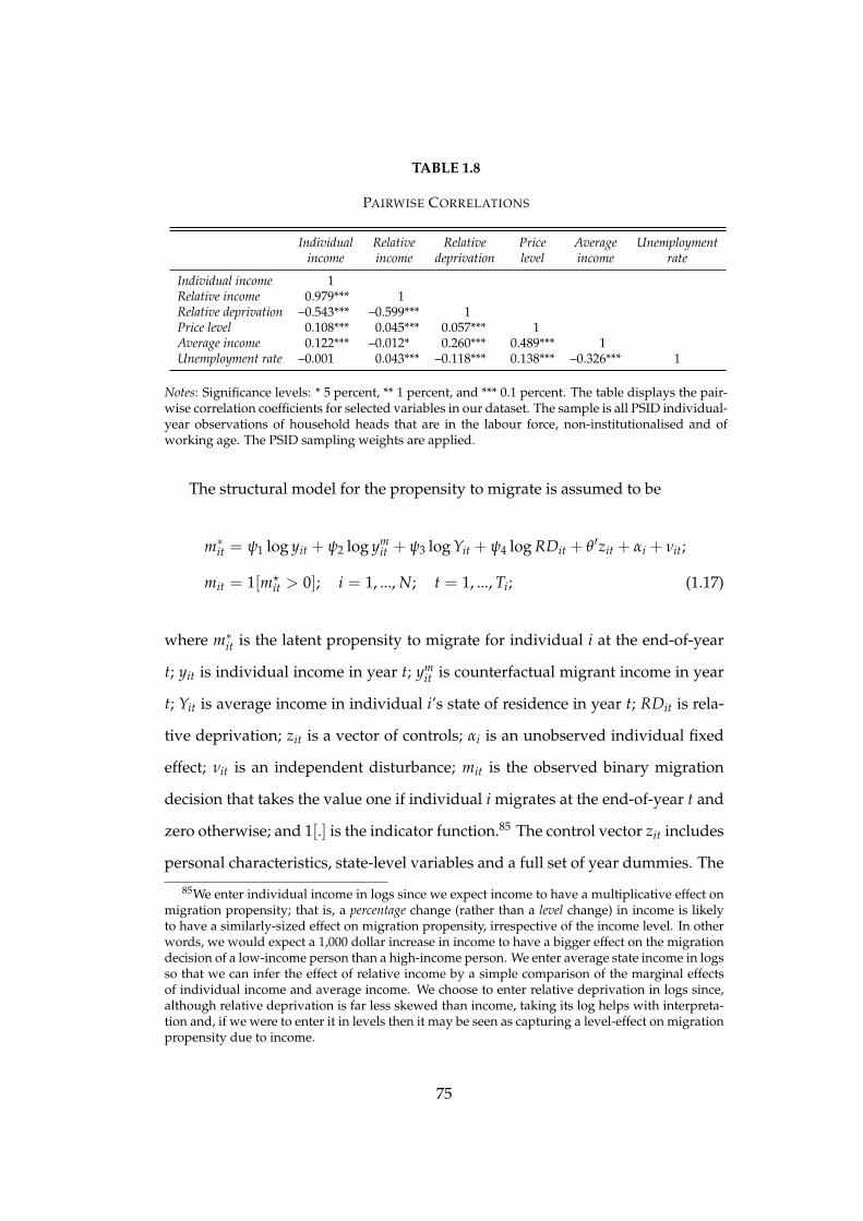
TABLE 1.8

PAIRWISE CORRELATIONS

Individual Relative Relative Price Average Unemploymentincome income deprivation level income rate

Individual income 1Relative income 0.979*** 1Relative deprivation –0.543*** –0.599*** 1Price level 0.108*** 0.045*** 0.057*** 1Average income 0.122*** –0.012* 0.260*** 0.489*** 1Unemployment rate –0.001 0.043*** –0.118*** 0.138*** –0.326*** 1

Notes: Significance levels: * 5 percent, ** 1 percent, and *** 0.1 percent. The table displays the pair-wise correlation coefficients for selected variables in our dataset. The sample is all PSID individual-year observations of household heads that are in the labour force, non-institutionalised and ofworking age. The PSID sampling weights are applied.

The structural model for the propensity to migrate is assumed to be

m∗it = ψ1 log yit + ψ2 log ymit + ψ3 log Yit + ψ4 log RDit + θ′zit + αi + νit;

mit = 1[m?it > 0]; i = 1, ..., N; t = 1, ..., Ti; (1.17)

where m∗it is the latent propensity to migrate for individual i at the end-of-year

t; yit is individual income in year t; ymit is counterfactual migrant income in year

t; Yit is average income in individual i’s state of residence in year t; RDit is rela-

tive deprivation; zit is a vector of controls; αi is an unobserved individual fixed

effect; νit is an independent disturbance; mit is the observed binary migration

decision that takes the value one if individual i migrates at the end-of-year t and

zero otherwise; and 1[.] is the indicator function.85 The control vector zit includes

personal characteristics, state-level variables and a full set of year dummies. The

85We enter individual income in logs since we expect income to have a multiplicative effect onmigration propensity; that is, a percentage change (rather than a level change) in income is likelyto have a similarly-sized effect on migration propensity, irrespective of the income level. In otherwords, we would expect a 1,000 dollar increase in income to have a bigger effect on the migrationdecision of a low-income person than a high-income person. We enter average state income in logsso that we can infer the effect of relative income by a simple comparison of the marginal effectsof individual income and average income. We choose to enter relative deprivation in logs since,although relative deprivation is far less skewed than income, taking its log helps with interpreta-tion and, if we were to enter it in levels then it may be seen as capturing a level-effect on migrationpropensity due to income.

75

personal characteristics we control for are age, age squared, a dummy for college

degree, marital status, number of children, and whether the individual is unem-

ployed or not at the time of the survey. The state-level variables we control for

are the price level, the unemployment rate, climatic conditions, number of bor-

dering states and land area. The parameters of primary interest are {ψ1, ψ3, ψ4},

which represent the causal effect of individual income, average income and rel-

ative deprivation on migration propensity, respectively. The question is, under

what conditions can we consistently estimate these parameters?

Causal inference relies on the regressors being exogenous; that is, statisti-

cally independent of the error term αi + νit (or as if the regressors were randomly

assigned to people). The error term represents all omitted variables that deter-

mine migration choice. For the (non-linear) panel random and fixed effects mod-

els that we will estimate, the parameter estimates are consistent only under the

assumption that the regressors are strictly exogenous (see Wooldridge (2002)).

Strict exogeneity requires the regressors to be uncorrelated with past, current

and future values of the error term. The problem is that income (and hence rel-

ative income and relative deprivation) is highly likely to be endogenous – that

is, there is feedback from migration choice to future income (and, hence, from

the error term to future income). Indeed, migrants would surely hope that mi-

gration has a positive effect on future income and the decision to migrate is in

large part in anticipation that migration will lead to higher income. There may be

other reasons why migration choice will affect income. Endogeneity is therefore

a problem that arises from not being able to observe all the factors that determine

migration choice. If we could control for all those variables that influence migra-

tion – including expected income conditional on migration – then there would

be no endogeneity concern because these variables will not be omitted from the

model. Indeed, the estimates are consistent under arbitrary dependence among

the regressors.

76

We take a number of steps towards consistent estimation. First, the regres-

sors are determined prior to the end-of-year migration decision; hence the re-

gressors are predetermined – that is, the unobserved disturbance is uncorrelated

with current and past values of the regressors, but may still be correlated with

future values.86 Second, we control for individual fixed effects, time effects and

a large vector of observable time-varying variables that have been suggested to

influence migration. Therefore, our estimates are consistent under arbitrary de-

pendence between the regressors and any unobserved time-invariant individ-

ual heterogeneity. The remaining source of endogeneity bias is if the regressors

are correlated with past values of the unobserved idiosyncratic (time-varying)

disturbance. We have already suggested that a ‘shock’ to migration choice is

likely to affect future income. Third and to reduce these ‘shocks’, we control for

predicted counterfactual migrant income that we estimated in the previous sec-

tion.87 Finally we present a series of robustness checks, including Wooldridge’s

(1997) estimator for the consistent estimation of non-linear fixed effects panel

data models without strict exogeneity.

Table 1.9 displays estimates for the average partial effects from a probit model

of equation (1.17), without controlling for relative deprivation (RDit). The aver-

age partial effect for a regressor tells us the change in the probability of migra-

tion for a one unit change in that regressor – for the typical individual in our

sample.88 Adjacent to the point estimate for the partial effect, the table reports

the corresponding standard error, which are bootstrapped, robust and clustered

86For example, if we observe that individual i resides in California in 1989, New York in 1990and New York in 1991, then mi1989 = 1 and mi1990 = 0. Personal characteristics (for example,college degree, marital status, unemployment status) refer to their values at the time of the PSIDsurvey within year t, whilst income refers to earnings in year t. There is no way that the individualcan retrospectively change the values of the regressors in response to their migration choice.

87Clearly we would not want to control for actual future income post-migration (which weobserve for migrants) because then it would be unclear what – if any – economic meaning wecould derive from this – the individual can never know for sure what his future income will be,individuals may make ‘mistakes’ when estimating their post-migration earnings.

88In computing the average partial effects, we set the individual-specific intercepts to zero –which is the mean of the random effects.

77

at the individual level.89

The first column of Table 1.9 controls for individual income, estimated mi-

grant income, average income and personal circumstances – whether unemployed,

age, age squared, whether college degree, whether married and number of chil-

dren. The partial effects are random effects estimates, that is, they assume the in-

dividual unobserved effect αi is uncorrelated with the regressors. The estimated

partial effect for individual income is insignificant (and has the wrong sign). A

priori, we would expect the partial effect of individual income to be negative

– under both the absolute and relative income hypotheses and holding average

income constant, an increase in absolute income (and, hence, relative income

too) reduces migration propensity. The effect of (counterfactual) migrant income

is also insignificant. In contrast, average income is positive and significant – a

one percent rise in average income increases the probability of migration by 1.2

percent, holding individual income constant. We also see that those who are un-

employed at the time of the survey are more likely to migrate; more specifically,

an unemployed person is .55 percent more likely to migrate than an employed

person. The estimates on the remaining controls are as expected. The probabil-

ity of migration is higher for people that are younger, with a college degree and

fewer children. The partial effect of being married is not statistically different

from zero. The estimated partial effect for age accounts for a quadratic in age.

We argued in section 1.3 that the random effects assumption – which is im-

plicit in the cross-sectional studies that dominate the related literature – is un-

likely to hold. The estimates in the second column of Table 1.9 display esti-

mates of the average partial effects from a probit fixed effects estimation us-

ing Mundlak’s (1978) correction procedure (see Mundlak (1978) and Wooldridge

(2002)).90 Mundlak (1978) assumes that the individual fixed effect, αi, can be89Bootstrapping should adjust the standard errors for the fact that counterfactual migrant earn-

ings are estimated.90The standard fixed effects methods for linear regression models (either differencing or group-

78

written as a linear function of the within-individual time mean of the regressors

and a disturbance term that is uncorrelated with the regressors. That is, αi =

a1 log yi + a2 log ymi + a3 log Yi + a′4zi + ci where the subscript i for the regressor

indicates the time mean for individual i, for example z1i ≡ T−1i ∑Ti

t=1 z1it, and ci is

a disturbance that is uncorrelated with the regressors (log yit, log ymi , log Yit, zit).

To estimate the model we simply run random effects estimation on the trans-

formed model that appends the within-individual time mean of the regressors to

the set of regressors.91

The fixed effects estimates in column two of Table 1.9 are very different from

the random effects estimates in column one. The partial effect on income is now

negative and significant, which conforms to prior expectations. A one percent

increase in individual income decreases the probability of migration by .034 per-

cent, which is small. The partial effect of average income is positive and even

higher than the estimate in column one – a one percent increase in average in-

come increases the probability of migration by 1.6 percent, holding individual

income constant. Migrant earnings remains insignificant. The partial effect of

a college degree in column two is lower than that in column one, which is not

surprising given that a college degree is likely correlated with unobserved innate

ability. The partial effect of marriage is now negative and significant.

If the random effects assumption that the fixed effect αi is uncorrelated with

the regressors is correct, then the coefficient estimates on the within-individual

time means of the regressors should not be significantly different from zero. The

vast majority of the individual time means of the regressors (not reported) are

demeaning) will not eliminate the fixed effect αi for the probit model. Further, directly estimat-ing the group-specific intercepts using Maximum Likelihood estimation leads to inconsistent esti-mates of the group intercepts – and consequently the slope coefficients too – since Ti is fixed andsmall (this is the ‘incidental parameters problem’, see Greene (2008)).

91In theory, zi should include the individual time means of the year dummies since, for ourunbalanced panel, the time means of the year dummies vary across individuals. However, doingso leads to convergence problems of the maximum likelihood solver; hence, the regression onlyincludes a full set of year dummies and not their individual time means.

79

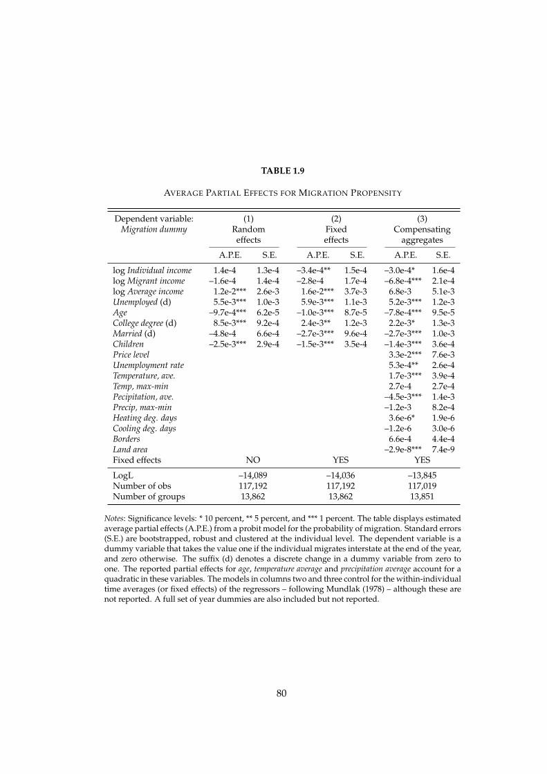
TABLE 1.9

AVERAGE PARTIAL EFFECTS FOR MIGRATION PROPENSITY

Dependent variable: (1) (2) (3)Migration dummy Random Fixed Compensating

effects effects aggregates

A.P.E. S.E. A.P.E. S.E. A.P.E. S.E.

log Individual income 1.4e-4 1.3e-4 –3.4e-4** 1.5e-4 –3.0e-4* 1.6e-4log Migrant income –1.6e-4 1.4e-4 –2.8e-4 1.7e-4 –6.8e-4*** 2.1e-4log Average income 1.2e-2*** 2.6e-3 1.6e-2*** 3.7e-3 6.8e-3 5.1e-3Unemployed (d) 5.5e-3*** 1.0e-3 5.9e-3*** 1.1e-3 5.2e-3*** 1.2e-3Age –9.7e-4*** 6.2e-5 –1.0e-3*** 8.7e-5 –7.8e-4*** 9.5e-5College degree (d) 8.5e-3*** 9.2e-4 2.4e-3** 1.2e-3 2.2e-3* 1.3e-3Married (d) –4.8e-4 6.6e-4 –2.7e-3*** 9.6e-4 –2.7e-3*** 1.0e-3Children –2.5e-3*** 2.9e-4 –1.5e-3*** 3.5e-4 –1.4e-3*** 3.6e-4Price level 3.3e-2*** 7.6e-3Unemployment rate 5.3e-4** 2.6e-4Temperature, ave. 1.7e-3*** 3.9e-4Temp, max-min 2.7e-4 2.7e-4Pecipitation, ave. –4.5e-3*** 1.4e-3Precip, max-min –1.2e-3 8.2e-4Heating deg. days 3.6e-6* 1.9e-6Cooling deg. days –1.2e-6 3.0e-6Borders 6.6e-4 4.4e-4Land area –2.9e-8*** 7.4e-9Fixed effects NO YES YES

LogL –14,089 –14,036 –13,845Number of obs 117,192 117,192 117,019Number of groups 13,862 13,862 13,851

Notes: Significance levels: * 10 percent, ** 5 percent, and *** 1 percent. The table displays estimatedaverage partial effects (A.P.E.) from a probit model for the probability of migration. Standard errors(S.E.) are bootstrapped, robust and clustered at the individual level. The dependent variable is adummy variable that takes the value one if the individual migrates interstate at the end of the year,and zero otherwise. The suffix (d) denotes a discrete change in a dummy variable from zero toone. The reported partial effects for age, temperature average and precipitation average account for aquadratic in these variables. The models in columns two and three control for the within-individualtime averages (or fixed effects) of the regressors – following Mundlak (1978) – although these arenot reported. A full set of year dummies are also included but not reported.

80

individually significantly different from zero. Moreover, a likelihood ratio test

between the nested models in columns one and two overwhelmingly rejects the

null hypothesis that the coefficients on the within-individual time means are

jointly insignificant. The likelihood ratio test statistic of 104 is far larger than

the critical value at the one percent level, 21.67.92 This suggests the fixed effects

model is the appropriate one. Therefore, this is evidence in support of our ear-

lier critique of cross-sectional studies; that is, unobservables (innate ability, mo-

tivation, willingness to move) play an important role in determining migration

propensity and are correlated with the regressors.

There is at least one obvious concern with the estimates in column two. If

the absolute income hypothesis has at least some relevance, then the (negative)

partial effect of individual income should be greater in absolute value than the

(positive) partial effect of average income – and if the pure relative income hy-

pothesis is correct then the partial effects on income and average income should

be equal in absolute value, which is overwhelmingly rejected. Clearly we need

to control for confounding state-level variables.

The estimates in column three of Table 1.9 control for various state-level vari-

ables. These are the state price level, unemployment rate, climatic conditions

(including a quadratic in average temperature and precipitation), number of bor-

dering states (a proxy for distance) and land area. Importantly, these state-level

controls render the partial effect of average income on migration choice insignif-

icant. The partial effect on individual income remains negative and significant.

Estimated migrant income is now significant but negative, which is the opposite

of what we would expect. The state price level has a positive and statistically

significant effect on the probability of migration. Recall that the price level is nor-

malised such that the average across states is one. Therefore, residing in a state

92The critical value of 21.67 is from the chi-squared distribution with 9 degrees of freedom.Recall that age is entered as a quadratic so there are 9 within-individual time means.

81

with a price level one percent higher than the average increases the probability of

migration by .033 percent compared to residing in a state with the average price

level. Therefore, the partial effect of the price level is comparable in magnitude

to that of individual income, which is what we would expect. Nonetheless, the

effect is small. Considering the remaining covariates, we see that the unemploy-

ment rate in the state of residence has a positive effect on migration propensity.

For the typical person a rise in average temperature increases the probability of

migration, whilst an increase in precipitation lowers migration propensity. Heat-

ing degree days – an indicator of the demand for heating – has a positive effect

on the probability of migration. The number of bordering states does not have a

significant effect; state land area reduces the probability of migration.

Table 1.10 contains the estimated average partial effects when we control for

relative deprivation. Holding individual income and average income constant,

it is possible to change relative deprivation. In section 3.2 we saw that a mean-

preserving spread of the income distribution can achieve this. Consider the es-

timates in column one, which does not control for average income. We see that

relative deprivation increases migration propensity – a one percent increase in

relative deprivation increases the probability of migration by about .18 percent.

This is economically significant given that only three percent of our observations

are when an individual migrates. The partial effects of individual income and

estimated migrant income are statistically insignificant.

The second column controls for relative deprivation and average income.

Both have a positive and significant effect on migration propensity, as predicted

by the relative income and relative deprivation hypotheses, respectively. The

coefficients on individual income and migrant income remain insignificant. In

the final column we control for the various state-level variables. As before, this

renders the effect of average income insignificant. However, the effect of relative

82

TABLE 1.10

AVERAGE PARTIAL EFFECTS FOR MIGRATION PROPENSITY:CONTROLLING FOR RELATIVE DEPRIVATION

Dependent variable: (1) (2) (3)Migration dummy Relative RD + Average Compensating

deprivation income aggregates

A.P.E. S.E. A.P.E. S.E. A.P.E. S.E.

log Individual income –5.8e-5 1.6e-4 –1.0e-4 1.6e-4 –5.5e-5 1.7e-4log Migrant income –2.7e-4 1.7e-4 –2.8e-4 1.8e-4 –6.8e-4*** 2.1e-4log Average income 1.3e-2*** 3.8e-3 3.8e-3 5.2e-3log Relative deprivation 1.8e-3*** 4.0e-4 1.5e-3*** 4.0e-4 1.6e-3*** 4.2e-4Unemployed (d) 5.8e-3*** 1.1e-3 5.8e-3*** 1.2e-3 5.1e-3*** 1.2e-3Age –9.6e-4*** 8.1e-5 –9.9e-4*** 8.8e-5 –7.7e-4*** 9.6e-5College degree (d) 3.0e-3** 1.2e-3 2.9e-3** 1.2e-3 2.6e-3** 1.3e-3Married (d) –2.5e-3*** 9.7e-4 –2.5e-3*** 9.7e-4 –2.6e-3** 1.0e-3Children –1.4e-3*** 3.5e-4 –1.4e-3*** 3.6e-4 –1.4e-3*** 3.7e-4Price level 3.4e-2*** 7.6e-3Unemployment rate 5.0e-4* 2.6e-4Temperature, ave. 1.7e-3*** 3.9e-4Temp, max-min 2.8e-4 2.7e-4Pecipitation, ave. –4.4e-3*** 1.4e-3Precip, max-min –1.2e-3 8.2e-4Heating deg. days 3.4e-6* 1.9e-6Cooling deg. days –1.3e-6 3.0e-6Borders 6.3e-4 4.4e-4Land area –2.9e-8*** 7.4e-9Fixed effects YES YES YES

LogL –14,031 –14,021 –13,831Number of obs 117,192 117,192 117,019Number of groups 13,862 13,862 13,851

Notes: Significance levels: * 10 percent, ** 5 percent, and *** 1 percent. The table displays averagepartial effects (A.P.E.) from a Mundlak (1978) fixed effects probit model. Standard errors (S.E.) arebootstrapped, robust and clustered at the individual level. The dependent variable is a dummyvariable that takes the value one if the individual migrates interstate at the end of the year, andzero otherwise. The suffix (d) denotes a discrete change in a dummy variable from zero to one. Thereported partial effects for age, temperature average and precipitation average account for a quadraticin these variables. All models include the individual-specific time averages for each regressor aswell as a full set of year dummies, but these are not reported.

83

deprivation is still positive and highly significant.

Robustness checks

Table 1.11 displays the results from various robustness checks. The columns

contain the average partial effects and corresponding standard errors for the two

regressors of primary interest: individual income and relative deprivation. The

baseline model is that in the third column of table 1.10 and – for ease of compar-

ison – we reproduce these estimates in the first row of table 1.11. The remaining

rows indicate a variant of the baseline model. Unless specified otherwise, all

estimations include the same controls as the baseline model.

The estimations in rows (2)–(4) add extra controls to the baseline model. As in

the baseline model, the figures are probit fixed-effects estimates using Mundlak’s

(1978) specification for the unobserved fixed effect. The second row controls for

whether the individual owns his or her own home. One may think that home

ownership has a direct effect on migration propensity since it increases the cost

of moving and, those that own their home tend not to be relatively deprived.

From the table we see that – compared to the baseline model – the partial effect

of relative deprivation is weakened slightly but it is still positive and significant.

A one percent rise in relative deprivation increases the probability of migration

by .11 percent for the typical individual. Home ownership has a strong negative

effect on migration propensity.

The estimates in the third row control for a full set of state dummies, which

take the value one if the individual is resident in that state and zero otherwise. If

there are state-level time-invariant factors that affect the attractiveness of a state

(such as amenities), then the state dummies will capture these. From the table

we see that this has no discernible effect on the estimates. A likelihood ratio test

84

TABLE 1.11

ROBUSTNESS CHECKS

Dependent variable: Individual RelativeMigration dummy income deprivation

Specification: A.P.E. S.E. A.P.E. S.E. LogL N

(1) Baseline –5.5e-5 1.7e-4 1.6e-3*** 4.2e-4 –13,831 117,019

Variable addition:(2) Control for whether –7.6e-5 1.8e-4 1.1e-3** 4.3e-4 –13,638 117,019

own home(3) State fixed effects –4.2e-5 1.8e-4 1.6e-3*** 4.3e-4 –13,748 117,019(4) Control for quartic 9.2e-4 2.3e-3 7.5e-3*** 2.7e-3 –13,790 117,019

in log income and RD(5) Enter everything in –4.1e-8** 1.6e-8 2.8e-7*** 7.4e-8 –13,807 117,019

levels, not logs

Sample selection:(6) Drop biennial obs. 2.6e-4 2.0e-4 1.6e-3*** 4.3e-4 –10,989 98,621(7) Movers –6.1e-4 1.3e-3 1.1e-2*** 2.9e-3 –9,690 27,411(8) Non-returning movers –6.9e-3*** 1.7e-3 1.0e-2** 4.1e-3 –4,058 12,852(9) Keep if income –2.4e-3*** 7.4e-4 4.9e-4 5.3e-4 –13,057 110,061

>$1,000(10) Keep if income –3.7e-8** 1.6e-8 3.6e-7*** 8.8e-8 –13,036 110,061

>$1,000 and entereverything in levels

(11) Keep if income 1.2e-2*** 3.4e-3 1.9e-2*** 3.9e-3 –13,020 110,061>$1,000 and controlfor quartic

(12) Keep if income 1.6e-4 1.8e-4 2.7e-3*** 6.2e-4 –13,482 114,543<$100,000

(13) Keep the 25 most 2.8e-5 2.1e-4 1.9e-3*** 5.1e-4 –11,123 97,827populous US states

(14) Drop self-employed –4.1e-5 2.1e-4 2.3e-3*** 5.2e-4 –12,853 104,986

Endogeneity tests:(15) Conditional FE logit –1.2e-7 4.4e-7 3.3e-6*** 1.0e-6 –6,469 25,718(16) Wooldridge (1997) –2.6e-2 2.7e-2 3.2e-1*** 7.7e-2 82,908

transform + GMM

Notes: Significance levels: * 10 percent, ** 5 percent, and *** 1 percent. The table displays averagepartial effects (A.P.E.) and corresponding standard errors (S.E.) for individual income and relativedeprivation. Standard errors are bootstrapped, robust and clustered at the individual level. Thedependent variable is a dummy variable that takes the value one if the individual migrates inter-state at the end of the year, and zero otherwise. Unless specified otherwise, all estimations includethe same controls as the baseline model in table 1.10, column 3. The final two columns report thelog likelihood and the number of observations (N). In row (15) the partial effect at the means isreported instead of the A.P.E., and row (16) reports the coefficient estimates and not the partialeffect.

85

firmly rejects the null hypothesis that the state fixed effects are jointly zero.

The estimation in the fourth row controls for a fourth-order polynomial in

log individual income and log relative deprivation. One may think that average

income and relative deprivation are capturing non-linearities in the effect of in-

dividual income on migration propensity. The estimates suggest this is not the

case.

In the fifth row we control for the levels of individual income, estimated mi-

grant income, average income and relative deprivation instead of their loga-

rithms. The partial effect of relative deprivation is positive and highly signifi-

cant. There is also evidence that absolute income matters too since the effect of

individual income is negative and significant at the five percent level.

In rows (6)–(14) we estimate the baseline model for selected subsamples to see

whether the results are driven by certain observations. In row six we drop all the

biennial observations. Recall, since 1997 the PSID has surveyed sample members

once every two years. This is problematic because the PSID asks respondents for

their labour income in the year prior to the survey. Our estimates suggest that

dropping the biennial observations does not affect the estimated partial effect of

relative deprivation.

The estimates in row seven use only the observations of individuals who in-

sample migrate interstate one or more times. If relative deprivation truly does

affect migration propensity then it should hold for the self-selected group of mi-

grants. Our estimates suggest this is the case and, moreover, the effect is eco-

nomically stronger for movers than for the full sample. A one percent increase in

relative deprivation increases the probability of migration by 1.1 percent, which

is substantial.

A possible concern is that the results may be driven by returning migrants

86

since it is typically thought that migrants return from high-income host states.

Row eight of table 1.11 presents estimates for when the sample is restricted to

in-sample interstate migrants who (in-sample) never return to either a state they

have previously resided in or to the state they grew-up. The partial effect of rel-

ative deprivation remains positive and significant at the five percent level. One

notable difference is that the effect of individual income is now statistically sig-

nificant and negative – as predicted by the absolute income theory. This would

seem to imply that whilst non-return migration is driven by bad income shocks,

return migration is not.

An interesting question is whether the unemployed are driving the results.

In row nine we restrict the sample to those observations where an individual

reports earnings in excess of 1,000 dollars (in 1999 prices). This renders the par-

tial effect of relative deprivation statistically insignificant, although the point es-

timate is positive. The effect of individual income is negative and significant.

Clearly the idea that relative deprivation matters for migration choice is less con-

vincing if its empirical relevance relies on the unemployed. It appears that the

functional form assumption may be important. More specifically, whilst we ex-

pect the logarithm of income to better capture the effect of income on migration

for the employed – and not the unemployed for whom a small increase in income

equates to a large percentage increase – differently we expect the logarithm of

relative deprivation to do a good job at capturing its effect for those with high

relative deprivation – and not the high earners. For a high earner, relative de-

privation is low and an additional small fall in the level of relative deprivation

equates to a large percentage decrease.

To assess this, row ten again restricts the sample to those earning over 1,000

dollars but this time enters everything in levels and not logarithms. The effect

of relative deprivation is positive and significant. In row eleven we control for

87

a fourth-order polynomial in log income and log relative deprivation – again for

the sample with income greater than a thousand dollars. The partial effect of rel-

ative deprivation is strongly positive and statistically significant – a one percent

increase in relative deprivation increases the probability of migration by almost

two percent. This point estimate is the highest of all the models considered. The

partial effect of income is significant but has the ‘wrong’ sign.

Another concern is income outliers at the top-end of the distribution. Some of

these extreme values may be due to typing errors – possibly adding one too many

digits. The estimates in row twelve use the subsample that drops all observations

where income is in excess of 100,000 dollars (in 1999 prices). The result is that,

compared to the baseline model, the partial effect of relative deprivation on the

probability of migration is higher.

Recall, when we compute relative deprivation for an individual, we use CPS

data on the earnings of individuals in the same state and year as that individual.

For smaller states the CPS sample size is small and possibly too small for reliable

estimation of relative deprivation. In row thirteen we restrict the sample to those

observations where the individual resides in one of the 25 most populous U.S.

states. Again the effect of relative deprivation is positive and significant. The

effect of average income is now significant but has the ‘wrong’ sign.

In row fourteen we exclude the self-employed from the sample. One may

think that the self-employed have different behavioural characteristics to those

who work for someone else – and, consequently, may have different slope co-

efficients. Dropping the self-employed increases the estimated average partial

effect of relative deprivation. The partial effect of individual income remains

statistically insignificant.

The remaining two rows of table 1.11 present estimates that attempt to do

more in terms of achieving consistent estimation of causal effects. Row fifteen

88

presents estimates from the logit conditional fixed-effects model of equation (1.17)

(see Chamberlain (1980)). The reason we do this is because, for the logit model,

Chamberlain (1980) showed that a sufficient statistic for the fixed effect (αi) exists.

Indeed, conditioning the likelihood of observing our data on ∑t mit eliminates αi

from the conditional likelihood function (see Greene and Hensher (2010)). There-

fore, we do not have to rely on Mundlak’s (1978) specification assumption for αi.

Unfortunately this comes at a cost since the resulting fixed effects model can only

be estimated for the subsample of movers.93 Therefore, in order to use the condi-

tional fixed effects estimates to say something about the whole population, one

needs to take a leap of faith and assume that the in-sample movers are not that

different from the stayers. The estimates displayed in row fourteen are partial ef-

fects evaluated at the mean of the regressors and not the average partial effect.94

The estimated partial effect for relative deprivation is positive and significant.

Of course we should still be concerned that the regressors are correlated with

past unobserved idiosyncratic disturbances. For example, this would occur if

a shock to the migration decision today affects future income. More generally,

any variable that is directly or indirectly chosen by an individual may not be

strictly exogenous. The literature on the estimation of non-linear fixed effects

panel data models without strict exogeneity is tiny. For consistent estimation when

the regressors are predetermined, Wooldridge (1997) extends the work of Cham-

berlain (1992) and proposes a quasi-differencing transformation and then Gen-

eralised Method of Moments (GMM) estimation of the resulting orthogonality

conditions.95

93The reason is that, for those who do not migrate in-sample, the value of the dependent vari-able is equal to zero in every period, which is perfectly explained by conditioning on ∑t mit.

94The conditional logit model will not give us estimates of the fixed effects that we require tocalculate the partial effects of the regressors. We follow the method proposed in Greene and Hen-sher (2010) to estimate the average fixed effect for the estimation sample and use this to calculatethe partial effect at the means. For our sample the estimated partial effect at the means is less thanthe average partial effect.

95To remove the fixed effect for a binary model, we need to assume a particular variant ofequation (1.17) such that the probability of migration can be factored into the product of a term

89

We assume that the predetermined regressors are individual income, pre-

dicted migrant income, relative deprivation, and the unemployed and college

degree dummies. The GMM estimation uses all the available lags of the pre-

determined regressors as instruments in a given year. We treat the remaining

regressors as strictly exogenous since these either can be considered determin-

istic (such as age) or they are state-level.96 We assume a logistic distribution for

the idiosyncratic error term. The estimates in row sixteen of table 1.11 display the

coefficient (not the partial effect) estimates from Wooldridge’s (1997) estimator.

The coefficient estimate on relative deprivation is positive and statistically signif-

icant. The coefficient estimate on individual income is negative but statistically

insignificant.

In summary, from studying interstate migration in the U.S., we have amassed

evidence in favour of Stark’s relative deprivation theory of migration. We find

little support for the absolute income theory that dominates the migration litera-

ture and the thinking of policy makers.

1.5 Concluding Remarks

This chapter has examined whether absolute income or relative income (to others

in some comparison group) provides the main motivation for migration. Almost

all models of migration – both theoretical and empirical – assume that absolute

income determines migration. Indeed, the most popular model of migration,

George Borjas’ (1987) selection theory, is built on the assumption that absolute

income differentials between the source and destination provide the incentive

that depends only on the fixed effect and a term that depends on the regressors. More specifically,rather than including the fixed effect αi in the expression for m?

it, we instead add the conditionthat migration occurs if the fixed effect is greater than some threshold (see Wooldridge (1997)).This may not be too restrictive since only certain types of people would even consider migration.There are some people that will never consider moving, no matter how large the income gain frommigration.

96An individual-level shock has a negligible effect on a state-level variable.

90

for migration. The model is so popular that a whole literature is devoted to

testing the migrant quality (or selection-on-skills) predictions of Borjas’ model,

and none of these papers control for relative income. All this is at odds with the

mounting evidence that suggests utility is driven by relative income (or relative

deprivation) as well as absolute income, particularly after a threshold level of

income – needed for the essentials in life – is exceeded.

We show that, under some conditions, the two main theories (absolute in-

come and relative deprivation) predict the same aggregate relationship between

income inequality and the quality (or selection-on-skills) of migrants. We argue

that in order to distinguish between the two theories, one needs individual-level

data. Moreover, one needs individual-level panel data on before and after mi-

gration outcomes. The reason is that, since migration and non-migration are

mutually exclusive, one has to estimate the (counterfactual) migrant earnings

of non-migrants using the subsample of migrant earnings. If migrants are se-

lected on unobservables, then cross-sectional estimates will systematically bias

the predicted migrant earnings of non-migrants. Importantly, we show that the

estimates are biased in favour of the finding that relative deprivation is impor-

tant precisely when migrants are positively selected-on-unobservables, which is

difficult to reconcile with the relative deprivation theory. Hence the need for

individual-level panel data to correct for selection-on-unobservables. Since the

current literature either fails to control for relative deprivation or fails to control

for selection-on-unobservables (or both), we undertake some empirical analysis

of our own.

The chapter estimates the relative importance of the two main theories in

explaining interstate migration in the United States. The data is a panel of indi-

viduals from the Panel Study of Income Dynamics. We assume that the reference

group to which income comparisons are made is the population of the U.S. state

91

of residence. First we find that for the subsample of migrants, their income and

relative deprivation both improve post-migration. Second, we jointly estimate

the effects of individual income and relative deprivation on the propensity to

migrate out of the source state. We find strong and robust evidence that an in-

crease in relative deprivation increases the probability of migration. In contrast,

our estimates suggest individual income has no significant effect on migration

propensity. This is true even after controlling for the estimated gain in income

from migration.

In studying U.S. interstate migration, we are looking at the migratory be-

haviour of people that – generally speaking – have enough income to buy the

‘essentials in life’, and hence are more likely to care about relative income than

those on very low incomes. Therefore, whether our findings have wider applica-

bility to regional migration in low-income countries, or international migration

(particularly between low- and high-income countries), should be the subject of

future research. Since in many cases of international migration the ‘essentials in

life’ are not satisfied, we would expect absolute income to be more important for

international migration.

On the one hand, our results are surprising given that the migration litera-

ture (and migration policy) is dominated by considerations of absolute income

differentials between the source and destination. On the other hand, our results

support the recent survey evidence that happiness is determined by relative in-

come (or deprivation), particularly when the average level of income is high.

There are several other promising avenues for future research. If, as we sug-

gest, relative deprivation is the correct theory of migration, then a big question

concerns how the reference group is chosen. Here we briefly discuss two aspects:

(1) what is the correct size (persons) of the reference group; and (2) how does the

reference group change in response to actions, including migration. Regarding

92

(1), we assume the reference group coincides with the population of a U.S. state,

but one may think that the true reference group is much narrower than this, par-

ticularly for the larger states.97 If the true reference group is narrower than the

state, then our estimate of the effect of relative deprivation on migration can be

seen as an underestimate. To see this, consider a state that contains a rich and

a poor neighbourhood. Assume that the inhabitants follow the relative depriva-

tion hypothesis. If the true reference group is the neighbourhood, then the rela-

tively deprived within each neighbourhood are more likely to migrate – either to

another neighbourhood within the same state or to another state. If, however, the

true reference group is the state, then the inhabitants of the poor neighbourhood

are more likely to migrate. Therefore, if the reference group is wrongly taken

to be the state rather than the neighbourhood, it works against our finding that

relative deprivation matters – the relatively deprived in the rich neighbourhood

are not deprived at the state level.

The second aspect concerns the endogeneity of the reference group. If rela-

tive deprivation matters, as we suggest, then an individual that migrates from a

poor to a rich region will surely do all he can to prevent reference substitution.

For example, this may require the migrant to avoid mixing with destination na-

tives and instead form social ties with earlier migrants from the same source.

If so, then one can expect enclaves and segregation. An interesting question is

whether leaving some family members behind in the source helps to prevent

reference group substitution? If so, it may provide a new explanation for remit-

tances, since it is a mechanism through which migrants avoid reference substi-

tution. Another question of interest is how the mere passing of time spent in the

destination affects the likelihood of reference substitution? If the probability of

reference substitution increases with time spent in the destination, then migrants

97Using population figures from the 2000 Census, one may be sceptical that a Californian com-pares himself to around 34 million other California residents, whereas a resident of Wyomingcompares himself to half a million.

93

may circle from source-to-destination-to-source and so on. Conversely, a migrant

from a rich source region will want to encourage reference substitution to that of

a lower-income destination. Migrants may then bring their families with them

and set up ties with natives in the destination. Furthermore, there are interest-

ing equilibrium aspects to be thought through. Clearly, the location decision of

one person changes the well-being of all persons in the source and destination

reference groups.

It is natural to question the unconventional. Many readers will ask, if rela-

tive income is so important for migration choice, why do we not see an exodus

from (high-income) New York to, say, (low-income) Louisiana? In response we

would say that our question is why we do not see the reverse flow. A Louisiana

janitor will probably earn more doing the same job in New York, but he or she

will likely be relatively more deprived in comparison to the high-income New

Yorkers. People trade-off the change in relative deprivation with the change in

income from migration and, on average, they tend to counter-balance each other.

One final comment. The existing evidence that finds well-being is determined

by relative income (or deprivation) – as well as absolute income – is from self-

reported happiness and life satisfaction. In contrast, we have revealed prefer-

ences that support the relative deprivation theory using the actual migration ac-

tions of individuals and, not subjective survey responses.98 Indeed, migration

provides excellent natural variation to assess relative deprivation. This is be-

cause relative deprivation can change substantially upon migration, particularly

when reference substitution occurs.99 More research needs to be done to assess98Naturally one may be sceptical as to whether survey respondents report their true feelings

when the question is subjective. Indeed, often a reordering of questions or a slight change in ques-tion wording can lead to a different answer (Bertrand and Mullainathan, 2001). Nonetheless, Freyand Stutzer (2002) present evidence to suggest that self-reported happiness is a reliable indicatorof well-being.

99Furthermore, the criticism that using migration data in this way is problematic since onecannot know the true reference group and how it changes after migration can equally be directedat the happiness literature.

94

the wider applicability of our result and, if our findings are confirmed, then an

evaluation of current migration and redistributive policy may be in order.

References

ABRAMITZKY, R., L. P. BOUSTAN, AND K. ERIKSSON (2011): “Leaving the nest:Lessons from 19th century Norway on migration and the childhood environ-ment,” Working paper, UCLA.

AMBROSINI, J. W. AND G. PERI (2011): “The Determinants and the Selection ofMexico-US Migrations,” Working paper, UC Davis.

ATEN, B. H. (2007): “Estimates of State Price Levels for Consumption Goods andServices: a first brush,” Working Paper 2007-06, Bureau of Economic Analysis.

AUTOR, D. H., L. F. KATZ, AND M. S. KEARNEY (2008): “Trends in U.S. WageInequality: Revising the Revisionists,” Review of Economics and Statistics, 90,300–323.

BASARIR, H. (2012): “Is it all relative? The role of wealth in the migration deci-sion: Evidence from Indonesia,” Working paper, University of York.

BERTRAND, M. AND S. MULLAINATHAN (2001): “Do People Mean What TheySay? Implications for Subjective Survey Data,” American Economic Review, 91,67–72.

BLANCHFLOWER, D. G. AND A. J. OSWALD (2000): “Well-being Over Time inBritain and the USA,” Working Paper 7487, NBER.

——— (2004): “Well-being over time in Britain and the USA,” Journal of PublicEconomics, 88, 1359–1386.

BLOOM, D. E. AND M. K. GUNDERSON (1991): “An Analysis of the Earnings ofCanadian Immigrants,” in Immigration, Trade, and the Labor Market, ed. by J. M.Abowd and R. B. Freeman, University of Chicago Press, 321–342.

BORJAS, G. J. (1985): “Assimilation, Changes in Cohort Quality, and the Earningsof Immigrants,” Journal of Labor Economics, 3, 463–489.

——— (1987): “Self-Selection and the Earnings of Immigrants,” American Eco-nomic Review, 77, 531–553.

——— (1991): “Immigration and Self-selection,” in Immigration, Trade, and theLabor Market, ed. by J. Abowd and R. Freeman, University of Chicago Press.

——— (1994): “The Economics of Immigration,” Journal of Economic Literature,32, 1667–1717.

95

BORJAS, G. J. AND B. BRATSBERG (1996): “Who Leaves? The Outmigration ofthe Foreign-Born,” Review of Economics and Statistics, 78, 165–176.

CHAMBERLAIN, G. (1980): “Analysis of Covariance with Qualitative Data,” Re-view of Economic Studies, 47, 225–238.

——— (1992): “Comment: Sequential moment restrictions in panel data,” Journalof Business and Economic Statistics, 10, 20–26.

CHIQUIAR, D. AND G. H. HANSON (2005): “International Migration, Self Se-lection, and the Distribution of Wages: Evidence from Mexico and the UnitedStates,” Journal of Political Economy, 113, 239–281.

CHISWICK, B. R. (1978): “The Effect of Americanization on the Earnings ofForeign-born Men,” Journal of Political Economy, 86, 897–921.

——— (1986a): “Human Capital and the Labour Market Adjustment of Immi-grants: Testing Alternative Hypotheses,” in Human Capital, Migration and De-velopment, ed. by O. Stark, Greenwich, CT: JAI Press, 1–26.

——— (1986b): “Is the New Immigration Less Skilled Than the Old?” Journal ofLabor Economics, 4, 168–192.

——— (1999): “Are Immigrants Favorably Self-Selected?” American EconomicReview, 89, 181–185.

CLARK, A. E., P. FRIJTERS, AND M. A. SHIELDS (2008): “Relative Income, Hap-piness, and Utility: An Explanation for the Easterlin Paradox and Other Puz-zles,” Journal of Economic Literature, 46, 95–144.

CLARK, X., T. J. HATTON, AND J. G. WILLIAMSON (2007): “Explaining U.S.Immigration: 1971-1998,” Review of Economics and Statistics, 89, 359–373.

DEATON, A. (2001): “Relative Deprivation, Inequality, and Mortality,” WorkingPaper 8099, NBER.

——— (2008): “Income, Health, and Well-Being around the World: Evidencefrom the Gallup World Poll,” Journal of Economic Perspectives, 22, 53–72.

DJAJIC, S. (1989): “Migrants In A Guest-Worker System - A Utility MaximizingApproach,” Journal of Development Economics, 31, 327–339.

DUESENBERRY, J. S., ed. (1949): Income, Saving and the Theory of Consumer Behav-ior, Cambridge, MA: Harvard University Press.

DUSTMANN, C. (1995): “Savings behavior of migrant workers: A life-cycle anal-ysis,” Zeitschrift fur Wirtschafts- und Sozialwissenschaften, 115, 511–533.

——— (2003): “Return Migration, Wage Differentials, and the Optimal MigrationDuration,” European Economic Review, 47, 353–369.

96

DUSTMANN, C. AND M. E. ROCHINA-BARRACHINA (2007): “Selection correc-tion in panel data models: An application to the estimation of females’ wageequations,” Journal of Econometrics, 10, 263–293.

DUSTMANN, C. AND Y. WEISS (2007): “Return Migration: Theory and EmpiricalEvidence from the UK,” British Journal of Industrial Relations, 45, 236–256.

EASTERLIN, R. A. (1974): “Does Economic Growth Improve the Human Lot?Some Empirical Evidence,” in Nations and Households in Economic Growth: Es-says in Honour of Moses Abramowitz, ed. by P. A. David and M. W.Reder, Aca-demic Press, New York, 89–125.

——— (1995): “Will raising the incomes of all increase the happiness of all?”Journal of Economic Behavior and Organization, 27, 35–47.

——— (2001): “Income and Happiness: Towards a Unified Theory,” EconomicJournal, 111, 465–484.

EASTERLIN, R. A., L. A. MCVEY, M. SWITEK, O. SAWANGFA, AND J. S. ZWEIG

(2010): “The happiness-income paradox revisited,” Proceedings of the NationalAcademy of Sciences of the United States of America, 107, 22463–22468.

ELDRIDGE, H. T. (1965): “Primary, Secondary, and Return Migration in theUnited States, 1955-60,” Demography, 2, 444–455.

FIELDS, G. S. (1982): “Place-to-Place Migration in Colombia,” Economic Develop-ment and Cultural Change, 30, 539–558.

FREY, B. S. AND A. STUTZER (2002): “What Can Economists Learn from Happi-ness Research?” Journal of Economic Literature, 40, 402–435.

GRAVES, P. E. (1980): “Migration and Climate,” Journal of Regional Science, 20,227–237.

GREENE, W. H., ed. (2008): Econometric Analysis, Englewood Cliffs, NJ: PrenticeHall.

GREENE, W. H. AND D. A. HENSHER, eds. (2010): Modeling Ordered Choices: APrimer, Cambridge, U.K.: Cambridge University Press.

GREENWOOD, M. J. (1975): “Research on Internal Migration in the United States:A Survey,” Journal of Economic Literature, 13, 397–433.

——— (1985): “Human Migration: Theory, Models, and Empirical Studies,” Jour-nal of Regional Science, 25, 521–544.

HARRIS, J. R. AND M. P. TODARO (1970): “Migration, Unemployment and De-velopment: A Two-Sector Analysis,” American Economic Review, 60, 126–142.

LAYARD, R., ed. (2005): Happiness: Lessons from a New Science, New York: Pen-guin.

97

LAYARD, R., G. MAYRAZ, AND S. NICKELL (2010): “Does Relative Income Mat-ter? Are the Critics Right?” in International Differences in Well-Being, ed. byE. Diener, J. Helliwell, and D. Kahneman, New York: Oxford University Press.

LIEBIG, T. AND A. SOUSA-POZA (2004): “Migration, Self-Selection and IncomeInequality: An International Analysis,” Kyklos, 57, 125–146.

LUTTMER, E. F. P. (2005): “Neighbors as Negatives: Relative Earnings and Well-Being,” Quarterly Journal of Economics, 120, 963–1002.

MEHLUM, H. (2002): “Should I Stay or Should I Go? On Relative Deprivationand Migration Dynamics,” Review of Development Economics, 6, 69–76.

MINCER, J., ed. (1974): Schooling, Experience and Earnings, New York: ColumbiaUniversity Press.

MUNDLAK, Y. (1978): “On the Pooling of Time Series and Cross Section Data,”Econometrica, 46, 69–85.

OTTAVIANO, G. I. AND G. PERI (2005): “Rethinking the gains from Immigration:Theory and Evidence from the U.S.” Working Paper 11672, NBER.

——— (2006): “Rethinking the Effects of Immigration on Wages,” Working Paper12497, NBER.

——— (2007): “The Effects of Immigration on U.S. Wages and Rents: A GeneralEquilibrium Approach,” Working Paper 13/07, CReAM.

QUINN, M. A. (2006): “Relative Deprivation, Wage Differentials and MexicanMigration,” Review of Development Economics, 10, 135–153.

RAIMON, R. L. (1962): “Interstate Migration and Wage Theory,” Review of Eco-nomics and Statistics, 44, 428–438.

RAMOS, F. (1992): “Out-Migration and Return Migration of Puerto Ricans,” inImmigration and the Workforce: Economic Consequences for the United States andSource Areas, ed. by G. J. Borjas and R. B. Freeman, University of Chicago Press,49–66.

ROY, A. D. (1951): “Some Thoughts on the Distribution of Earnings,” OxfordEconomic Papers, 3, 135–146.

SCHULTZ, T. P. (1982): “Lifetime Migration within Educational Strata inVenezuela: Estimates of a Logistic Model,” Economic Development and CulturalChange, 30, 559–593.

SEMYKINA, A. AND J. M. WOOLDRIDGE (2010): “Estimating panel data modelsin the presence of endogeneity and selection,” Journal of Econometrics, 157, 375–380.

98

SJAASTAD, L. A. (1962): “The Costs and Returns of Human Migration,” Journalof Political Economy, 70, 80–93.

STARK, O. (1984): “Rural-to-Urban Migration in LDCs: A Relative DeprivationApproach,” Economic Development and Cultural Change, 32, 475–486.

——— (1991): The Migration of Labor, Cambridge, MA: Basil Blackwell.

——— (2006): “Inequality and migration: A behavioral link,” Economics Letters,91, 146–152.

STARK, O., C. HELMENSTEIN, AND Y. YEGOROV (1997): “Migrants Savings, Pur-chasing Power Parity, and the Optimal Duration of Migration,” InternationalTax and Public Finance, 4, 307–324.

STARK, O. AND J. E. TAYLOR (1989): “Relative Deprivation and InternationalMigration,” Demography, 26, 1–14.

——— (1991): “Migration Incentives, Migration Types: The Role of Relative De-privation,” The Economic Journal, 101, 1163–1178.

STARK, O. AND Y. Q. WANG (2000): “A theory of migration as a response torelative deprivation,” German Economic Review, 1, 131–143.

——— (2005): “Towards a theory of self-segregation as a response to relativedeprivation: steady-state outcomes and social welfare,” in Economics and Hap-piness: Framing the Analysis, ed. by L. Bruni and P. L. Porta, Oxford: OxfordUniversity Press.

STARK, O. AND S. YITZHAKI (1988): “Labour Migration as a Response to Rela-tive Deprivation,” Journal of Population Economics, 1, 57–70.

STEVENSON, B. AND J. WOLFERS (2008): “Economic Growth and SubjectiveWell-Being: Reassessing the Easterlin Paradox,” Brookings Papers on EconomicActivity, 2008.

STOUFFER, S. A., E. A. SUCHMAN, L. C. DEVINNEY, S. A. STAR, AND R. M.WILLIAMS JR., eds. (1949): Studies in Social Psychology in World War II: TheAmerican Soldier. Vol. 1, Adjustment During Army Life, Princeton: Princeton Uni-versity Press.

TODARO, M. P. (1969): “A Model of Labor Migration and Urban Unemploymentin Less Developed Countries,” American Economic Review, 59, 138–148.

WILKINSON, R. G., ed. (1996): Unhealthy societies: the afflictions of inequality, Lon-don: Routledge.

WOOLDRIDGE, J. M. (1995): “Selection corrections for panel data models underconditional mean independence assumptions,” Journal of Econometrics, 68, 115–132.

99

——— (1997): “Multiplicative panel data models without the strict exogeneityassumption,” Econometric Theory, 13, 667–678.

——— (2002): Econometric Analysis of Cross Section and Panel Data, Cambridge,MA: MIT Press.

YITZHAKI, S. (1979): “Relative deprivation and the gini coefficient,” QuarterlyJournal of Economics, 93, 321–324.

100

Appendix

Appendix 1.A Sample and Variable Construction for the

Empirical Analysis

This appendix describes the construction of the sample and the variables used in

the empirical analysis of section 1.4.

The Sample

The sample is from the Panel Study of Income Dynamics (PSID). The PSID con-

tains two separate data sets: an individual file with longitudinal data on every

individual that has ever appeared in the PSID; and a family file for each cross-

sectional year that contains information on the head, “wife” and family unit for

all family units sampled in that year. The family files contain the vast major-

ity of survey information, while the individual file is needed to keep track of a

specific individual because of moves into and out of different family units. Im-

portantly, both the individual file and family file contain the year, family-unit,

and relationship-to-head identifiers, which combined permit us to link the two

data sets.100

We merge the files in the following way. First, we reshape the individual file

into long format; that is, each row now contains a unique individual-year iden-

tifier. Second, we download the family files for all survey years into a single

100Note that when we say relationship-to-head we do not mean that we directly use the variable“Relationship to head” as given in the PSID individual file. Indeed, the PSID variable “Relation-ship to head” is not sufficient to identify the current head because any last year’s head (or wife)that moved out is also recorded as the head (wife) in this variable. As the PSID documentationexplains, the current head is identified by yearly values for “Sequence Number” in the range 1-20and a value for “Relationship to head” of either 1 or 10. The current “wife” is identified by yearlyvalues for “Sequence Number” in the range 1-20 and a value for “Relationship to head” of either2, 20, or 22. In 1968 we can safely identify the head with “Relationship to head”=1 and wife with“Relationship to head”=2 because, trivially, there are no movers in the first year of the sample.

101

file and reshape it into long-long format so that each row is either a head-year,

“wife”-year or family-year observation. We then merge the family file with the

individual file in three steps. First, we merge based on year-family-head and

year-family-wife for all head and wife observations, respectively. Secondly, we

merge based on year-family for all current period family unit variables. Finally,

we merge based on year–family–non-split-off–non-mover for all family unit vari-

ables that are lagged one period; for example, the survey question on family

income asks retrospectively what family income was in the prior period. A prob-

lem arises when the head, for example, moved families between the prior and

current period, since merging based on year-family-head will incorrectly allocate

family income to the wrong head. Hence, we merge the lagged family-level data

only for those family members who did not change families between the prior

and current period. These are non-split-off families and non-mover individuals.

Our working sample includes people that meet all of the following four cri-

teria:

1. The head of household is typically the adult male head (the husband if

married) unless an adult male is not present or is severely disabled. The current

head is identified jointly by yearly values for “Sequence Number” in the range

1-20 (PSID variable ER30021 in 1969) and a “Relationship to head” value of 1

or 10 (PSID variable ER30003 in 1968). The sequence number is used to ensure

that only the current head is included and not the head in the previous wave in

the event that the previous head moved out of the household. In 1968 we can

safely identify the head with a “Relationship to head” value 1 because there are

no movers in the first period.

2. Of working age is defined as those persons aged between 16 and 64.

3. In the labour force is determined by looking at the employment status

of the head from the family files. Prior to 1976, employment status was coded

102

using six values (PSID variable V196 in 1968), where the labour force are those

with values 1 or 2. Between 1976 and 1996 there were eight values, where the

labour force are those with values 1-3. Since 1996 respondents were offered more

than one mention to describe their employment status. We use the first mention

(PSID variable ER10081 in 1997).

4. Non-institutionalised individuals are people that are not in either the

armed forces, prison, a health care or educational facility. We drop those in the

armed forces using occupation. Members of the armed forces have occupation

code 55 in the 2-digit classification (variable V4459 in 1976), code 600 in the 1970

Census Occupation Codes (COC) (PSID variable V7712 in 1981), and code 984

in the 2000 COC (PSID variable ER21145 in 2003). We also use type of institu-

tion for the family unit (variable V11124 in 1985) to determine when a family is

institutionalised, which includes those in the armed forces living off base.

The Dependent Variables

End-of-period migration is a dummy variable that takes the value one if the in-

dividual changes state between the current and next survey, and zero otherwise.

The state of residence is recorded in the PSID family file. Prior to 1985, states

were coded according to the GSA classification (variable V93 in 1968) and from

1985 classified using the FIPS system (variable V12380 in 1985). We converted

the FIPS codes to the GSA classification. There are instances where an individual

has a gap between records because of non-response or missing values. When the

gap is more than two years we set the end-of-year migration decision to missing

(which is the case for 1.5 percent of observations).

End-of-period return migration is a dummy that takes the value one if the

individual returns to a state he previously resided in between the current and

next survey, and zero otherwise. We keep track of all states an individual has

103

previously resided in within sample and, in addition, the PSID records the state

the individual grew-up (defined as where the individual spent most of his years

between the ages of 6 and 16). Prior to 1994 the grew-up state was coded using

the GSA classification (variable V311 in 1968) and since 1997 using the FIPS code

(variable ER11842 in 1997).

The Regressors

Individual income includes wages, bonuses, overtime, commissions and the labour

part of business and farm income (PSID variable V74 in 1968) and refers to to-

tal annual income before tax in the previous year to the survey. In the years

1994-1996 and 2001, labour income was reported excluding the labour part of

business and farm income. For these years we construct total labour income by

summing labour income excluding business and farm income (variable ER4140

in 1994), farm income (ER4117 in 1994) and the labour portion of business income

(ER4119 in 1994). Labour income is expressed in constant 1999 dollars using the

CPI-U. Survey respondents are asked about their labour income in the previous

year. We lag labour income by one survey wave to account for this although it is,

of course, imperfect for the biennial surveys post-1997.

Average income is the sample mean income from the Current Population Sur-

vey in a given state-year, where the sample is restricted to those in the labour

force. The income series includes wages and salaries and is expressed in 1999

dollars.

Unemployed is a dummy variable that takes the value one if the individual

is unemployed at the time of the PSID survey, and zero otherwise. From the

employment status variable (PSID variable V196 in 1968), the unemployed have

code 2 for years prior to 1976 and code 3 since 1976.

104

Own home is a dummy variable that takes the value one if the individual

owns their home and zero otherwise. This is determined by looking at the value

of the house (PSID variable V5 in 1968), which is coded zero if the individual is

not a home owner.

Age of an individual is reported in the PSID in each survey (PSID variable

ER30004 in 1968). We take the first recorded age of the individual and apply the

gap in survey years to fill in age over time. We do this to avoid the sporadic

two-year jumps or no change in reported age between surveys that sometimes

occur due to changes in the date of the survey within a year.

College degree is a dummy variable that takes the value one if the individual

has a Bachelor’s degree (1968-1974 we use PSID variable with name V313 in 1968;

1975-2009 we use PSID variable with name V4099 in 1975).

Married is a dummy variable that takes the value one if the individual is

married at the time of the PSID survey and zero otherwise. We use the married

pairs indicator from the individual file (PSID variable ER30005 in 1968).

Children is the number of children under 18 living in the family unit at the

time of the PSID survey (PSID variable V398 in 1968).

Borders is the number of contiguous U.S. states for the state that the individ-

ual resides.

Land area of a state is obtained from the U.S. Census Bureau and is measured

in square kilometres.

Sampling weights

Sampling weights are inverse (ex-ante) sampling probability weights supplied

by the PSID. From 1968 to 1989 we use the “Core Individual Weight” (vari-

105

able ER30019 in 1968); 1990-1992 the “Combined Core-Latino Weight” (ER30688

in 1990); 1993-1995 the “Combined Core-Latino Sample Longitudinal Weight”

(ER30866 in 1993); 1996 we use the “Core Sample Individual Longitudinal Weight”

(ER33318) and post-1996 we use the “Combined Core-Immigrant Sample Indi-

vidual Longitudinal Weight” (ER33430 in 1997).

106

Chapter 2

Wealth, Intertemporal Choice and

Return Migration

2.1 Introduction

It is well-known that many migrants eventually return to their source.1 The phe-

nomenon is known as return migration.2 To take an example from the 2000 U.S.

Census, between 1995 and 2000 a total of 107,961 people moved to Puerto Rico

from the United States (U.S.) mainland. Of these, 66 percent were born in Puerto

Rico and, of the remainder, 56 percent reported Puerto Rican origin.3 The cross-

sectional Census does not allow us to determine the proportion of migrants that

return; however, we know that – between 1995 and 2000 – for every two people

that moved from Puerto Rico to the US mainland, roughly one person moved in

the opposite direction, which is suggestive that return migration is very large.

1Throughout this chapter we will use ‘source’ to refer to the region that an individual grew upin and, ‘host’ to refer to any region other than the source.

2Return migration is the flow from the ‘host’ to the ‘source’ region.3More precisely, 107,961 people resided on the U.S. mainland in 1995 and lived in Puerto Rico

in 2000. Therefore, this is a lower bound for those that moved from the mainland to Puerto Ricobetween 1995 and 2000.

107

Return migration is neither specific to nor unusually large in Puerto Rico.

Looking at all interstate migration between 1995 and 2000 (again from the 2000

Census), roughly 20 percent of all interstate migrants are returning to their state

of birth. Nor is it specific to internal migration, evidence abounds for the return

of international migrants.4 Several theories have been proposed to explain this.

However, it has not been shown analytically that these hypotheses can actually

generate return migration. Therefore, the purpose of this chapter is to show that,

under some conditions, a number of these theories can generate optimal return

migration.

Why is it important? Migration generally commands much public and po-

litical attention and return migration accounts for a large slice of two-way mi-

gration. At the most basic level, understanding the causes of return migration

can help forecast population totals and their characteristics in the source and

host. Indeed, we do not yet have a good grasp of the determinants of migration

and, even less so, return migration. Consequently, whilst natural increase can be

planned for, migration is often seen as a shock. Return migrants – by definition –

stay in the host temporarily as opposed to permanently and, therefore, it is likely

that their impact on the source and host region will differ from that of perma-

nent migrants. Indeed, we will show that the actions of return migrants in the

host and source will depend critically on the reason for return migration. In or-

der to understand return migration, a first step is to show analytically that some

of the theories that have been proposed to explain migration can actually gen-

erate return migration by optimising individuals. An analytical model will also

help to build intuition for the result and characterise the conditions needed for

return migration as well as the consumption, saving, and hours worked choices

of return migrants.

4See, for example, Dustmann (1996) on the large-scale post-war temporary migrations to Cen-tral Europe.

108

At least six hypotheses have been proposed to explain the return migration

phenomenon. The first five of these all require that the (expected) nominal wage

is higher in the host region than the source region. In addition, one or more

of the following should hold: (1) location-specific marginal utility and a higher

marginal utility of consumption in the source (Hill, 1987, Djajic and Milbourne,

1988, Raffelhschen, 1992, Yang, 2006); (2) a cheaper cost of living in the source

than the host (or a higher purchasing power of the host country currency in the

source country) (Djajic, 1989, Dustmann, 1995, 1997, 2003, Stark et al., 1997, Dust-

mann and Weiss, 2007); (3) relative deprivation and a lower average income (or

consumption) in the source (Stark, 1991); (4) uncertainty and ‘mistakes’ about

economic conditions in the host region (Borjas and Bratsberg, 1996); and (5) im-

perfect capital markets in the source may encourage temporary migration to ac-

cumulate savings for setting up a business upon return (Ilahi, 1999, Mesnard,

2004, Yang, 2006). The final explanation, which does not require a higher wage in

the host, is (6) spending time in the host region increases human capital (through

education or experience) which raises wages upon returning home (Dustmann,

1995, 1997, Borjas and Bratsberg, 1996, Dustmann and Weiss, 2007). There is very

little empirical evidence to suggest which, if any, of these theories is correct.5

We build a tractable, two region model of migration that can embody the

first three of these hypotheses. That is, migrants have location-specific marginal

utility of consumption, price levels in the source and host may differ, and a differ-

ence in average consumption between the source and host can also be captured.

In the model, consumers decide whether to never migrate, permanently migrate,

5Mesnard (2004) did not find much evidence of human capital accumulation for Tunisian re-turn migrants (20% of return migrants accumulated education whilst abroad and only 8% used itupon return to Tunisia). Ilahi (1999) finds that Pakistani return migrants were able to enter self-employment upon return facilitated by their accumulated savings from their time spent abroad(see also McCormick and Wahba (2000) for Egypt, and Woodruff and Zenteno (2007) for Mexico).Yang (2006) tests the prediction that migrants return when they have reached a certain amount ofsavings by looking at the effect of movements in the exchange rate. Yang concludes that migrantstend to stay longer when the source currency weakens, suggesting a life-cycle model rather thanmigration to accumulate a certain amount of money.

109

or return migrate. The model explains return migration from an ex-ante expec-

tation (or intention) to return to the source, it is not based on ‘mistakes’ or bad

luck post-migration.6 Most theoretical models of migration are static and, there-

fore, assume migration is permanent (see, for example, Borjas (1987)). Those that

have modelled return migration have sought to derive the optimal duration in

the host conditional on returning at some point (Dustmann, 2003). In contrast,

we will show that, under some conditions, return migration is optimal compared

to the corner solutions of never migrating and permanently migrating.

The rest of the chapter is organised as follows. Section 2.2 presents the model

and shows analytically that, under some conditions, return migration is optimal.

Section 2.3 concludes. All proofs are contained in the appendix.

2.2 The Model

We make the following assumptions. An individual lives for finite T periods.

There are two regions: North (N) and South (S). Let j ∈ {N, S} index the current

region of residence. Individual nominal income in region j, yj, is assumed to be

constant. The period utility function, u(c, j), is a function of consumption (c > 0)

and the region of current residence (j). We assume utility is homogeneous of de-

gree (1− γ) in consumption, where γ > 0. The marginal utility of consumption

is positive but diminishing: uc > 0, ucc < 0. We assume the individual has a

non-pecuniary preference for one region over the other; more specifically,

u(c, S) = κu(c, N); ∀c, (2.1)

6In a survey of the return migration literature, Gmelch (1980) notes that few studies advanceunfavourable economic conditions in the host region as the trigger for return migration.

110

where κ > 0 is the non-pecuniary cost of residing in the North region. The cost

is positive when κ > 1 and negative (a benefit) when κ < 1.7,8 Under the ho-

mogeneity of the utility function, κ1

1−γ can be thought of as the gross percentage

change in consumption required to leave the individual indifferent between re-

siding in the North and the South. Notice that the non-pecuniary cost of residing

in the North is incurred each period.

The non-pecuniary cost, κ, is a modelling tool that can capture a number of

different preferences. First, κ can capture relative attachment to the South that

may arise because the individual was born and raised in the South, has a famil-

iarity with the South and the existence of social networks in the South, or simply

likes the amenities available in the South. Second, κ can proxy for preferences

that exhibit a relative consumption (or ‘keeping up with the Joneses’) motive

where the Joneses in the North and South differ in their consumption level.9

Third, κ can represent preferences for a particular climate; a desire for the warm

Southern climate could be modelled by specifying κ > 1. It is likely that κ is het-

erogeneous and time-varying as a result of the individual’s actions. For example,

the length of time spent in a region and whether, say, the individual gets married

to a native in the host region will likely impact κ. However, for tractability we

will assume κ is time-invariant.7This assumption is similar to that made in Raffelhschen (1992) and Dustmann and Weiss

(2007), although Raffelhschen interprets κ as capturing all possible costs of migration – tangibleand intangible. Since κ is incurred each period spent in the North rather than a one-off cost,we view it as an non-pecuniary (intangible) cost rather than a (tangible) monetary moving cost.In contrast to Raffelhschen (1992) we allow for spending some time in each location rather thanpermanency. We differ from Dustmann and Weiss (2007) in that we model the choice betweenswitching (an interior solution) and permanent migration (a corner solution) explicitly.

8It is important that κ enters multiplicatively with u(c, N) rather than additively because wewant κ to affect the marginal utility of consumption. One could assume that κ is consumption-augmenting such that the non-pecuniary cost is measured in terms of compensating consumption.However, then, in order for κ > 1 to lower the utility of any given consumption in the North wewould have to constrain γ ∈ (0, 1), which means the substitution effect dominates the incomeeffect and this is a restriction we do not want.

9For example, for the constant relative risk-aversion utility function u(c, j) = φ1(j=S)

Cjc1−γ/(1−

γ) where 1(.) is the indicator function, φ measures attachment to the South and Cj is average

consumption in region j; then κ =φCNCS

.

111

It is a key assumption of the model that κ enters multiplicatively with the

utility function in equation (2.1). Consequently, the marginal utility of consump-

tion is higher in the non-pecuniary preferred region for all levels of consumption.

We assume perfect capital markets, no time-discounting and a zero net interest

rate.10,11,12 Finally, there is no uncertainty, no legal restrictions to migration and

no monetary costs of moving (or one can think of income in the host as net of

moving costs).13

Let Pj denote the (constant) aggregate price level in region j = N, S. The

individual flow budget constraint in period τ is

ωτ+1 =

ωτ − PScτ + yS if j = S

ωτ − PNcτ + yN if j = N,

where ω is cash-in-hand (or wealth).

2.2.1 Location strategies

With discrete choice models such as migration, we need to impose substantial

structure (constraints) on location choice to keep things tractable.14

10Hence, there is no liquidity constraint motive for migration.11Since we are primarily concerned with how migration affects the consumption choice around

trend we assume perfect capital markets and a flat consumption path in the absence of migration.12Notice that, even though markets are complete, the presence of κ means that maximizing

utility is not equivalent to first maximizing income and then smoothing consumption. Indeed,when yN > yS and κ > 1, the individual faces a trade off between income maximisation and thenon-pecuniary cost of residing in the North. We abstract from incomplete markets to keep themodel tractable, although clearly this is a deficiency.

13The lack of uncertainty does not imply that uncertainty is not relevant, rather it is our wish toshow that switching can occur even in the absence of uncertainty. It would seem that uncertaintywould reduce outmigration for risk-averse agents but, conditional on migration, it may increasereturn migration when a bad outcome is realized. Migration flows, income differentials and un-employment rates across regions are highly persistent, which suggests uncertainty cannot be themain factor. In a survey of the return migration literature, Gmelch (1980) notes that few studiesadvance unfavourable economic conditions in the host region as the trigger for return migration.

14If any timing of migration were permitted then one quickly finds that having to rank a num-ber of alternatives makes the problem intractable.

112

The assumptions we have made mean that the choice of the individual is

simply a choice between three location strategies: (1) permanently reside in the

South; (2) permanently reside in the North; and (3) spend a fraction σ ∈ (0, T− 1)

of one’s lifetime in the North and a fraction T−σ in the South, where σ is endoge-

nous. The reason is that, under our assumptions, the individual is indifferent be-

tween any combination of moves that adds up to a fraction σ of the individual’s

lifetime spent in the North. This indifference occurs because, by assumption, the

key variables yN , yS and κ are constant, there is no physical cost of migration and

we have perfect capital markets. In the switching case, neither the timing nor the

number of moves is pinned down. That said, for the purposes of comparing per-

manent migration to return migration, it will be useful to impose that migrants

move immediately upon turning adult at time 0 and then the switchers in our

model are akin to return migrants.15

The existing theoretical literature has not classified the parameter space over

which an individual would ex-ante choose to switch rather than permanently

reside in a particular region. Instead, the literature has focused on the optimal

time to return migrate (or switch) conditional on returning. In what follows we

look to characterize the location decision as a function of initial wealth, κ and the

income differential. The aim is to show that the switching (or return) migration

strategy is optimal for some of the parameter space.

Consider the value to the individual of either permanently residing in the

North or the South. The value of an individual that resides in region j from

period 0 until death in period T − 1 (T periods) is the solution to

Vj(ω0) = max{cτ}T−1

τ=0

{u(cτ, j)− λ

[Pj

T−1

∑τ=0

cτ − Tyj −ω0

]},

15An interesting extension would be to allow κ to depend on σ. This would endogenise κ by,say, letting the source bias depreciate with time spent in the host region and/or for the externalhabit reference group to be a weighted average of mean consumption in the two regions wherethe weights are σ and T − σ.

113

where λ is the marginal value of income and the term in square brackets is the

lifetime budget constraint. Clearly the individual chooses to perfectly smooth

consumption over time, cτ = 1Pj

[yj +

ω0T

], ∀τ ∈ {0, 1, ..., T − 1}. Then, the value

of permanently residing in the North is

VN(ω0) = Tu(

1PN

[yN +

ω0

T

], N)

, (2.2)

and the value of permanently residing in the South is

VS(ω0) = Tu(

1PS

[yS +

ω0

T

], S)

= κTu(

1PS

[yS +

ω0

T

], N)

, (2.3)

where the second equality uses equation (2.1) to express VS(ω0) in terms of utility

from (counterfactually) residing in the North.

Consider now the value of an individual in period 0 conditional on spending

a fraction σ ∈ (0, T − 1) of the individual’s life in the North and a fraction T − σ

in the South, where σ is endogenous. The value function is given by

VR(ω0) = maxσ,{cτ}T−1

τ=0

[σ−1

∑τ=0

u(cτ, N) +T−1

∑τ=σ

u(cτ, S)

−λ

(PN

σ−1

∑τ=0

cτ + PS

T−1

∑τ=σ

cτ − σyN − (T − σ)yS −ω0

)].

As written, the time index in the above formulation implies that the switching

individual resides in the North for the first σ periods of his life and then resides

in the South for the remaining T − σ periods. The first-order-conditions equate

114

the marginal utility of consumption across time; that is,

cτ = cτ+1 if τ ∈ {0, 1, ..., σ− 2, σ, σ + 1, ..., T − 2}

uc(cτ, N) = PNPS

uc(cτ+1, S) if τ = σ− 1.

(2.4)

From (2.1), the homogeneity of degree (1− γ) and ucc < 0 it follows that cσ =(PNPS

κ) 1

γ cσ−1. From the intertemporal budget constraint, we find the consump-

tion function

cτ =

1

PN

(ω0+σyN+(T−σ)yS

σ+(T−σ)κ

)if τ ∈ {0, 1, ..., σ− 1}

1PS

κ(

ω0+σyN+(T−σ)ySσ+(T−σ)κ

)if τ ∈ {σ, σ + 1, ..., T − 1}

, (2.5)

where κ ≡(

PNPS

) 1−γγ

κ1γ . Let cN and cS denote consumption of a switcher while

in the North and South, respectively. The following proposition follows imme-

diately from equation (2.5).

Proposition 2.2.1 When PNPS

κ > 1, switchers consume less each period while residing

in the North than while residing in the South, and vice versa. If PNPS

κ > 1 and γ < 1,

switchers have lower expenditure and higher saving when in the North than in the South.

If PNPS

κ > 1 and γ > 1, the difference in the expenditure and saving of switchers between

the North and South is ambiguous.

The ambiguity arises due to γ, the inverse elasticity of intertemporal substi-

tution. When γ < 1, the substitution effect dominates the income effect of a price

change, expenditure will be lower and saving higher in the North compared to

the South when PNPS

κ > 1. When γ > 1 there is a high willingness to smooth con-

sumption, the income effect of a price change dominates and the difference in a

switcher’s expenditure and saving between the North and South is ambiguous.

115

Later we will show that switching itself requires a high elasticity of intertemporal

substitution, and hence it is likely that switchers will save while in the host.

It is well-known that there is a strong positive correlation between prices and

income (the Penn effect). Therefore, conditional on return migration to a low-

income low-price region, return migrants are likely to save while in the host and

dissave upon returning home. Many authors have shown that price differentials

and a source bias individually entice saving in the host region and dissaving

upon return to the source region. This fits in well with anecdotal evidence that

return migrants save whilst in the host and spend after returning to their source

region (Gmelch, 1980).

The following proposition is trivial yet necessary for completeness.

Proposition 2.2.2 ∀κ ∈ (0, 1] and yN > yS, VN(ω0) > VR(ω0) > VS(ω0); and

∀κ ∈ [1, ∞) and yN < yS, VN(ω0) < VR(ω0) < VS(ω0).

Proposition 2.2.2 simply says that an individual optimally chooses to reside

permanently in the North when both nominal income is higher in the North than

the South and there exists a non-pecuniary benefit or price differential favouring

the North, and vice versa. Clearly then, if switching is optimal, there must be a

trade-off between the income differential and the non-pecuniary cost.

For switchers, the first-order condition with respect to σ equates the loss of

utility from extending the stay in the North by one period with the gain in utility

from the additional consumption that can be afforded by staying in the North an

extra period; that is,

u(cS, S)− u(cN , N) = σuc(cN , N)∂cN

∂σ+ (T − σ)uc(cS, S)

∂cS

∂σ. (2.6)

Proposition 2.2.3 Conditional on switching being optimal, the fraction of lifetime spent

116

in the North region is

σ =

[(1− γ)κyN − (κ − γ)yS − γ(κ − 1)ω0

T(yN − yS)(κ − 1)

]T, (2.7)

where κ ≡(

PNPS

) 1−γγ

κ1γ .

As expected, σ is decreasing in initial wealth ω0 when yN > yS, and vice

versa. The reason is that a necessary condition for switching is κ > 1 (a prefer-

ence for the South) when yN > yS, and higher wealth is better spent in the South

where there is a higher marginal utility of consumption. The effect of an increase

in PNPS

is to unambiguously reduce σ; similarly a rise in κ reduces σ if γ < 1.16

We will show later that for switching to be optimal, γ – the inverse elasticity of

intertemporal substitution – has to be low. The effect of a change in yN and yS on

σ is a little more complex. Consider the case κ > 1 and yN > yS. Then, σ is de-

creasing in yS because the income and substitution effects of the income change

work in the same direction. In contrast, the effect of a rise in yN on σ is ambigu-

ous because the substitution effect is positive and the income effect is negative

(see Djajic and Milbourne (1988), Dustmann (2003) and appendix B of Mesnard

(2004)).17 That said, given yN > yS, an increase in yN will reduce σ unless initial

wealth is very negative (ω0 < −TyS).18

2.2.2 Location decision rule

We return now to the question of which of the three location strategies – per-

manently reside in the South, permanently reside in the North, or switch – is

optimal. From proposition 2.2.2 it remains for us to consider the two cases

16 ∂σ∂κ = − T(1−γ)

(κ−1)2 , ∂σ

∂PNPS

= (1−γ)κ

γPNPS

∂σ∂κ , ∂σ

∂κ = κγκ

∂σ∂κ .

17In the case when yN > yS, we can sign the partials ∂σ∂yS

= − γ(yN−yS)2 [TyN + ω0] < 0; and

∂σ∂yN

= Tκ(1−γ)−(κ−1)σ(yN−yS)(κ−1) = γ

(yN−yS)2 [TyS + ω0] ≷ 0.18The terminal condition ensures initial wealth ω0 > −[σyN + (T − σ)yS].

117

{κ > 1, yN > yS} and {κ < 1, yN < yS}. In what follows, we focus on the

case {κ > 1, yN > yS}, the converse can be obtained via a simple change of vari-

ables. The following proposition establishes a unique crossing point for any pair

of conditional value functions.

Proposition 2.2.4 The partial derivatives of the conditional value functions with re-

spect to ω0 are ranked as

∂VS(ω0)

∂ω0>

∂VR(ω0)

∂ω0>

∂VN(ω0)

∂ω0> 0,

for all κ > 1, yN > yS, and for any admissible ω0.

The ranking of partial derivatives of the conditional value functions with re-

spect to wealth emits a 3-tuple of unique cut-off values for initial wealth such that

the individual is indifferent between any two of the three location strategies. Let

z1 denote initial wealth such that VS(z1) = VN(z1). Similarly, let VS(z2) = VR(z2)

and VN(z3) = VR(z3). The following proposition provides a ranking of the cut-

offs for initial wealth.

Proposition 2.2.5 z3 < z1 if and only if z2 > z1; and z3 > z1 if and only if z2 < z1.19

19Burdett (1978) proves this in the context of job search.

118

It is straightforward to show the cut-off values are,

z1 =T(yN − κ

γ1−γ yS)

κγ

1−γ − 1, (2.8)

z2 =[σ(z2) + (T − σ(z2))κ]

γ1−γ [σ(z2)yN + (T − σ(z2))yS]− T

11−γ κ

γ1−γ yS

Tγ

1−γ κγ

1−γ − [σ(z2) + (T − σ(z2))κ]γ

1−γ

,

(2.9)

z3 =T

11−γ yN − [σ(z3) + (T − σ(z3))κ]

γ1−γ [σ(z3)yN + (T − σ(z3))yS]

[σ(z3) + (T − σ(z3))κ]γ

1−γ − Tγ

1−γ

,

(2.10)

where z2 and z3 are implicit functions and σ(z) denotes the value of σ evaluated

at ω0 = z. An explicit solution for z2 and z3 can be derived (see appendix) for

the special case γ = 0.5,

z2 = T[

κ(yN − yS)

κ − 1− yS

], (2.11)

z3 = −T[

yN −yN − yS

κ − 1

]. (2.12)

A corollary of propositions 2.2.4 and 2.2.5 is that the switching strategy is

admissible only when z2 > z1. Proposition 2.2.6 states that this is always the

case when the inverse elasticity of substitution is sufficiently low.

Proposition 2.2.6 z2 > z1 for all κ > 1, yN > yS, γ ∈ (0, 1). Hence, for any given

κ > 1, yN > yS and γ ∈ (0, 1), there exists a ω0 such that the switching strategy is

optimal.

Figure 2.1 presents an illustration of the conditional value functions under

propositions 2.2.4 - 2.2.6. We see that individuals with low initial wealth (ω0 <

z3) migrate permanently to the North, and those with a high initial wealth (ω0 >

z2) never migrate away from the South, all else equal. Return migrants (or

119

switchers) have an initial wealth in the middle range (z3 < ω0 < z2).

FIGURE 2.1

CONDITIONAL VALUE FUNCTIONS

ω0z3 z2z1

VS(ω0)

VR(ω0)

VN(ω0)

Notes: The figure illustrates the value to an individualof permanently residing in the South, VS(ω0), perma-nently residing in the North, VN(ω0), or return migrat-ing, VR(ω0), as a function of initial wealth ω0. Themodel assumes that the individual earns a higher incomein the North than the South and the individual has a non-pecuniary preference for the South.

The following proposition characterises the parameter space over which switch-

ing is optimal.

Proposition 2.2.7 For any given initial wealth ω0, switching occurs when both κ andyNyS

are individually large and∣∣∣ yN

yS− κ − x∗

∣∣∣ small, where x∗ = (κ−1)ω0TyS

.

Figure 2.2 graphs the optimal location strategy given ω0 = 0 and γ = 0.5 as a

function of κ and yN/yS. We see that return migration (or switching) is optimal

when there is jointly a large income differential and a high non-pecuniary pref-

erence for the region with the lower income (or, alternatively, lower prices in the

region with the lower income).

120

FIGURE 2.2

OPTIMAL LOCATION DECISION RULE

1.1 1.2 1.3 1.4 1.5 1.6 1.7 1.8 1.9 2

1.2

1.4

1.6

1.8

2

2.2

2.4

2.6

2.8

3

κ

yN

/yS

Switching −Strategy

South

North

Notes: The figure plots the individual migration decisionspace. On the vertical axis is the non-pecuniary costof residing in the North (κ) and on the horizontal axisis the North-South income ratio. The shaded area la-belled ‘South’ refers to permanently residing in the South,‘North’ refers to permanently residing in the North, andthe ‘Switching strategy’ is akin to return migration. Thefigure assumes the individual has zero initial wealth andan elasticity of intertemporal substitution equal to two.

121

It is clear that, given a North-South income differential and a non-pecuniary

preference for the South, return migration is optimal if the elasticity of intertem-

poral substitution (EIS) is sufficiently high. In the limit as the EIS tends to infinity,

return migration is always optimal.

Proposition 2.2.8 For any given initial wealth, switching becomes more prevalent when

the elasticity of intertemporal substitution, 1/γ, increases. In the limit as γ tends to zero,

switching is optimal for all κ > 1, yN > yS.

2.3 Conclusion

This chapter has examined some of the proposed explanations for return migra-

tion. In particular, we present an analytical model of migration choice in the

presence of location-dependent marginal utility of consumption, an income dif-

ferential and a difference in the cost of living between the source and host region.

In propositions 2.2.4 - 2.2.7 we derive the optimal location decision rule from a

restricted set of strategies: permanently reside in the South, permanently reside

in the North, or migrate and subsequently return to the source. We mapped the

parameter space under which return migration (or switching) is optimal. For re-

turn migration to occur a necessary condition is that there exists a non-pecuniary

preference for (or lower prices in) the region with the lower nominal income. We

find that return migration is more prevalent when the non-pecuniary preference

and the income differential are jointly large. If either one of these is small while

the other is large then one tends to get either permanent migration or no migra-

tion at all. Also, initial wealth is a key factor. Those individuals turning adult

with few assets are more likely to migrate and high-asset individuals are likely to

stay in the region they grew up in. Conditional on migration, those with higher

assets are more likely to return to the region they grew up in. These are novel

122

predictions which can be tested empirically.

References

BORJAS, G. J. (1987): “Self-Selection and the Earnings of Immigrants,” AmericanEconomic Review, 77, 531–553.

BORJAS, G. J. AND B. BRATSBERG (1996): “Who Leaves? The Outmigration ofthe Foreign-Born,” The Review of Economics and Statistics, 78, 165–176.

BURDETT, K. (1978): “A Theory of Employee Job Search and Quit Rates,” Ameri-can Economic Review, 68, 212–220.

DJAJIC, S. (1989): “Migrants In A Guest-Worker System – A Utility MaximizingApproach,” Journal of Development Economics, 31, 327–339.

DJAJIC, S. AND R. MILBOURNE (1988): “A General Equilibrium Model of Guest-Worker Migration: The Source Country Perspective,” Journal of InternationalEconomics, 25, 335–351.

DUSTMANN, C. (1995): “Savings behavior of migrant workers: A life-cycle anal-ysis,” Zeitschrift fur Wirtschafts- und Sozialwissenschaften, 115, 511–533.

——— (1996): “Return Migration – The European Experience,” Economic Policy,22, 214–250.

——— (1997): “Return migration, uncertainty and precautionary savings,” Jour-nal of Development Economics, 52, 295–316.

——— (2003): “Return Migration, Wage Differentials, and the Optimal MigrationDuration,” European Economic Review, 47, 353–369.

DUSTMANN, C. AND Y. WEISS (2007): “Return Migration: Theory and EmpiricalEvidence from the UK,” British Journal of Industrial Relations, 45, 236–256.

GMELCH, G. (1980): “Return Migration,” Annual Review of Anthropology, 9, 135–159.

HILL, J. K. (1987): “Immigrant Decisions Concerning Duration of Stay and Mi-gratory Frequency,” Journal of Development Economics, 25, 221–234.

ILAHI, N. (1999): “Return migration and occupational change,” Review of Devel-opment Economics, 3, 170–186.

MCCORMICK, B. AND J. WAHBA (2000): “Overseas work experience, savingsand entrepreneurship amongst return migrants to LDCs,” Scottish Journal ofPolitical Economy, 48, 164–178.

123

MESNARD, A. (2004): “Temporary migration and capital market imperfections,”Oxford Economic Papers, 56, 242–262.

RAFFELHSCHEN, B. (1992): “Labor migration in Europe: Experiences from Ger-many after unification,” European Economic Review, 36, 1453–1471.

STARK, O. (1991): The Migration of Labor, Cambridge, MA: Basil Blackwell.

STARK, O., C. HELMENSTEIN, AND Y. YEGOROV (1997): “Migrants Savings, Pur-chasing Power Parity, and the Optimal Duration of Migration,” InternationalTax and Public Finance, 4, 307–324.

WOODRUFF, C. AND R. ZENTENO (2007): “Migration networks and microenter-prises in Mexico,” Journal of Development Economics, 82, 509–528.

YANG, D. (2006): “Why Do Migrants Return To Poor Countries? Evidence FromPhilippine Migrants Responses To Exchange Rate Shocks,” Working Paper12396, NBER.

124

Appendix

Appendix 2.A Proofs

Proof of Proposition 2.2.2 We show that permanently residing in the North is preferred to the

switching strategy for all κ ≤ 1, yN > yS. To do this, rewrite VR as

VR(ω0) = σu(cN , N) + (T − σ)u(cS, S)

= σu(cN , N) + (T − σ)κu

((PNPS

κ

) 1γ

cN , N

)

= σu(cN , N) + (T − σ)κu(cN , N)

= [σ + (T − σ)κ] u(cN , N)

< Tu(

1PN

[yN +

ω0T

], N)= VN(ω0).

where the inequality arises because [σ + (T − σ)κ] < T and cN < 1PN

[yN + ω0

T]. A symmetric

argument can be used to show that permanently residing in the South is preferred to the switching

strategy for all κ ≥ 1, yN < yS.

Proof of Proposition 2.2.3 From (2.6) we have

u(cS, S)− u(cN , N) = σuc(cN , N)∂cN∂σ

+ (T − σ)uc(cS, S)∂cS∂σ

⇔ [uc(cS, S)cS − uc(cN , N)cN ]

1− γ= σuc(cN , N)

∂cN∂σ

+ (T − σ)uc(cS, S)∂cS∂σ

(2.13)

⇔[cS − PN

PScN ]

1− γ= σ

PNPS

∂cN∂σ

+ (T − σ)∂cS∂σ

(2.14)

⇔ cN1− γ

[

(PNPS

) 1−γγ

κ1γ − 1] =

∂cN∂σ

[σ + (T − σ)

(PNPS

) 1−γγ

κ1γ ]

=

(yN − yS

PN

)− (1−

(PNPS

) 1−γγ

κ1γ )cN (2.15)

⇔ cN

γ

((PNPS

) 1−γγ

κ1γ − 1

)1− γ

=

(yN − yS

PN

)

where (2.13) follows from homogeneity of degree 1− γ of the utility function, (2.14) follows from

125

the first order condition for consumption in (2.4), and (2.15) follows from the consumption func-

tion in (2.5). After substituting for cN using (2.5) and rearranging it follows

σ =

[(1− γ)κyN − (κ − γ)yS

(yN − yS)(κ − 1)

]T − γ

(yN − yS)ω0,

where κ ≡(

PNPS

) 1−γγ

κ1γ .

Proof of Proposition 2.2.4

∂VS(ω0)

∂ω0=

κ

PSuc

(1PS

[yS +

ω0T

], N)

=1

PNuc

(κ−1 1

PN

[yS +

ω0T

], N)

,

∂VR(ω0)

∂ω0=

1PN

uc(cN , N) +∂VR(ω0)

∂σ

∂σ

∂ω0

=1

PNuc(cN , N) (2.16)

∂VN(ω0)

∂ω0=

1PN

uc

(1

PN

[yN +

ω0T

], N)

,

where equation (2.16) follows from the first-order condition ∂VR(ω0)∂σ = 0. The arguments of the

marginal utility functions above are ranked

κ−1 1PN

[yS +

ω0T

]=

1PN

(ω0 + TyS

Tκ

)<

1PN

(ω0 + TyS

σ + (T − σ)κ

), ∀κ > 1 (2.17)

<1

PN

(ω0 + σyN + (T − σ)yS

σ + (T − σ)κ

), ∀yN > yS

≡ cN

<1

PN

(ω0 + TyN

σ + (T − σ)

), ∀κ > 1, yN > yS (2.18)

=1

PN

[yN +

ω0T

].

Proposition 2.2.4 follows from ucc < 0. To be precise, we need a restriction on ω0 for the inequal-

ities to hold. The inequality in (2.17) requires ω0 > −TyS and the inequality in (2.18) requires

ω0 > − T(κyN−yS)κ−1 < −TyN . Since lifetime income cannot exceed TyS in the South and TyN in the

North, the constraint on initial wealth is implied by the terminal condition ωT = 0.

Proof of Proposition 2.2.5 If z2 > z1, from Proposition 2.2.4 this implies VR(z1) > VS(z1) ⇒

VR(z1) > VN(z1) ⇒ z1 > z3. If z3 < z1, from Proposition 2.2.4 this implies VN(z1) < VR(z1) ⇒

126

VS(z1) < VR(z1) ⇒ z2 > z1. The last statement of Proposition 2.2.5 follows from similar reason-

ing.

Derivation of z2 and z3 when γ = 0.5 Substituting for σ in (2.9) using (2.7) and setting γ = 0.5 it

follows

0.25(κ− 1)2z22−T(0.5yS + 0.5κyN− κyS)(κ− 1)z2 = T2

[κyS(yN − yS)(κ − 1)− 0.25(κyN − yS)

2]

.

Complete the square to obtain

(z2 −

T(0.5yS + 0.5κyN − κyS)

0.5(κ − 1)

)2= T2

[κyS(yN − yS)(κ − 1)− 0.25(κyN − yS)

2

0.25(κ − 1)2

]+ T2

[(0.5yS + 0.5κyN − κyS)

2

0.25(κ − 1)2

]= 0.

Therefore z2 = T[

κ(yN−yS)κ−1 − yS

]. Similarly, substituting for σ in (2.10) using (2.7) and setting

γ = 0.5 it follows

0.25(κ− 1)2z23 +T(0.5yS +(0.5κ− 1)yN)(κ− 1)z3 = T2

[yN(yN − yS)(κ − 1)− 0.25(κyN − yS)

2]

.

Complete the square to obtain

(z3 +

T[0.5yS + (0.5κ − 1)yN ]

0.5(κ − 1)

)2= T2

[yN(yN − yS)(κ − 1)− 0.25(κyN − yS)

2

0.25(κ − 1)2

]+ T2

[[0.5yS + (0.5κ − 1)yN ]2

0.25(κ − 1)2

]= 0.

Therefore z3 = −T[yN −

yN−ySκ−1

].

Proof of Proposition 2.2.6 It is easiest to show z2 > z1 in the special case γ = 0.5. From (2.8) and

(2.11), z2 > z1 if and only if

(κ − 1)(yN − yS) > 0,

which holds for all κ > 1, yN > yS. In the general case where γ ∈ (0, 1), z2 > z1 if

[σ + (T − σ)κ]γ

1−γ [σ(κγ

1−γ − 1) + T]− T1

1−γ κγ

1−γ > 0.

The last part of Proposition 2.2.6 follows from Proposition 2.2.5.

127

Proof of Proposition 2.2.7 Again it is easiest to show this for the special case γ = 0.5. The switch-

ing location strategy is optimal if and only if z2 > ω0 and z3 < ω0, which from (2.11) and (2.12)

requires

max{(

2− yNyS

)κ − 1 +

(κ − 1)ω0TyS

, (2− κ)yNyS− 1− (κ − 1)ω0

TyS

}< 0.

To see what this implies for κ and yNyS

, set the two arguments of the max function equal to get:yNyS− κ = (κ−1)ω0

TyS≡ x∗. Notice x∗ is increasing in ω0. Consider now three cases depending on

ω0. First, when ω0 = 0, the two arguments of the max function are mirror images in yNyS

and

κ. Therefore, for switching to take place, yNyS

and κ need to be close enough, that is(

yNyS− κ)

close to x∗ = 0. Substituting yNyS

= κ into the max function shows that the function is negative

and, hence, switching is optimal for all κ > 1, yN > yS. If yNyS

< κ, then the first argument of

the max function dominates and switching requires(

2− yNyS

)κ < 1, that is yN

ySlarge enough and

κ − yNyS

small enough. If yN/yS > κ, then the second argument of the max function dominates

and switching requires (2− κ)yNyS

< 1, that is κ large enough and yNyS− κ small enough. Second,

when ω0 > 0, then x∗ is positive and yNyS− κ must not get too far away from this positive x∗ for

switching to occur. Third, when ω0 < 0, then x∗ is negative and yNyS− κ must not get too far away

from this negative x∗ for switching to occur.

For the general case γ ∈ (0, 1), numerical solution suggests the proposition still holds.

Proof of Proposition 2.2.8 We will show that limγ→0 z2 = +∞ and limγ→0 z3 = −TyN . From

equation (2.7) divide the numerator and denominator by κ and take the limit to get

limγ→0

σ = limγ→0

[(1− γ)yN − (1− γ

κ )yS − γ(1− 1κ )

ω0T

]T

(yN − yS)(1− 1κ )

= T,

because limγ→0 κ = +∞. This is not a surprising result, when γ = 0 utility is linear in consump-

tion so the individual optimally spends almost all his time in the North where income is higher,

he saves and only consumes when in the South, which is just one period. Now we want to find

the limit of the term [σ + (T − σ)κ]γ

1−γ . Using equation (2.7) we have

[σ + (T − σ)κ]γ

1−γ =

[Tγ(κyN − yS + (κ − 1)ω0

T)

(yN − yS)

] γ1−γ

.

128

The limit of the term in square brackets is determined by

limγ→0

[κyN − yS + (κ − 1)ω0

T]

1/γ=

+∞+∞

= limγ→0

− 1γ2

(yN + ω0

T)

κ log(

PNPS

κ)

− 1γ2

= +∞,

where the second equality applies L’Hopital’s rule. Using this result we can show limγ→0 [σ + (T − σ)κ]γ

1−γ =

PNPS

κ by taking the logarithm and applying L’Hopital’s rule as follows

limγ→0

log[

σ + (T − σ)κ1−γ

γ

]1−γ

γ

=+∞+∞

= limγ→0

[1γ +

(yN+ω0T )κ log

(PNPS

κ)(− 1

γ2

)[κyN−yS+(κ−1) ω0

T ]

](− 1

γ2

)

= limγ→0

−γ +log(

PNPS

κ)

1−[

yS+ω0T

(yN+ω0T )κ

]

= log(

PNPS

κ

).

Now the limits of z2 and z3 follow immediately

limγ→0

z2 =T PN

PSκ(yN − yS)

PNPS

κ − PNPS

κ= +∞

limγ→0

z3 = −TyN( PN

PSκ − 1)

PNPS

κ − 1= −TyN

For completeness, it is easy to show that limγ→0 z3 < limγ→0 z1 < limγ→0 z2, ∀yN > yS, κ > 1

since 20

limγ→0

z1 =T(

yN − PNPS

κyS

)PNPS

κ − 1.

Finally, from the homogeneity of degree 1− γ in consumption assumption of the utility function,

we have uccc = −γuc, so the utility function exhibits constant relative risk-aversion − ucccuc

= γ

and the intertemporal elasticity of substitution equals 1/γ.

20Note that κ > 1⇒ PNPS

κ > 1 for γ = 0.

129

Chapter 3

Place Attachment, Job Search and

Migration: a Structural

Estimation

“There is for virtually everyone a deep association with and con-sciousness of the places where we were born and grew up, where welive now, or where we have had particularly moving experiences.”- Edward Relph (1976, p.43) “Place and Placelessness”

3.1 Introduction

The emotional attachment a person feels towards the place (or area) he or she

inhabits is often mentioned as an important obstacle to migration; however, it

has rarely been studied empirically.1,2 The term ‘place attachment’ originates

1We define migration as a change in the place of his or her main residence for a period of atleast a year. This is consistent with the United Nation’s definition of a migrant.

2A number of theoretical papers on the determinants of migration assume utility depends onplace attachment in some form. Most of these study return migration (see, for example, Hill (1987),Djajic and Milbourne (1988), Raffelhschen (1992), Dustmann (2003), Mesnard (2004), Yang (2006),Dustmann and Weiss (2007)). To generate an incentive for return migration, these papers assume

130

from psychology. It refers to the emotional bonds and feelings one has with an

area. These bonds typically form and develop through spending time in a place,

and are directly related to practical considerations such as social networks, a

familiarity with surroundings and amenities. A number of papers have found

distance-to-destination to have a large negative effect on the probability of mi-

gration to that destination (see, for example, Sjaastad (1962)). The consensus is

that the monetary costs of moving would have to be implausibly large to ex-

plain this. Therefore, the literature has tended to attribute the adverse effect of

distance on migration to either increasing (with distance) information costs or

increasing (with distance) ‘psychic’ costs (Schwartz, 1973). In addition to the

costs associated with distance, it seems likely that there is a fixed cost (indepen-

dent of distance) of leaving the place that one currently resides. That is, place

attachment determines the number of persons at risk of migration as well as the

choice among potential destinations, where the latter is conditional on migration.

Since place attachment is – by its psychological nature – largely unobservable, we

know very little about its level and variation across individuals and time. The

purpose of this chapter is, therefore, to examine how the component of place

attachment that is independent of distance-to-destination is formed and, to es-

timate its variation in the population of the United States using panel data on

interstate migration.

Economically, it is crucial that we understand and quantify place attachment

if we are to better forecast the volume and timing of migration. Indeed, the num-

ber of people at risk of migration critically depends on place attachment. Data

from the U.S. Current Population Survey, 1999-2011, shows that the numbers

that migrate each year are significant. The first row of Table 3.1 displays the

percent of persons that moved in the last year, by type of migration. On aver-

utility is non-separable in consumption and place attachment, implying place attachment affectsthe marginal utility of consumption (and possibly leisure too). In contrast, we assume utility islinear and separable in income and place attachment.

131

age, each year around seven percent move within a county, two percent move

across county borders within a state, two percent move across state boundaries,

and 0.4 percent move from abroad. There are several other reasons why policy

makers would want to quantify place attachment. First, proponents of migration

point to migration as a valve for the labour market: in bad times – when there

is unemployment – migrants tend to leave and in good times – when labour de-

mand exceeds supply – there tends to be immigration. Place attachment is an

obstacle to this. Clearly then we would like to know the distribution of place at-

tachment in the population. In particular, what percentage are at risk of moving

for a given change in economic conditions? Second, we would like to know the

time (or duration) dependence of place attachment. Conditional on migration,

theoretically it is unclear whether place attachment will increase or decrease with

duration in the destination. Intuitively there is a trade-off between homesickness

(from leaving the source) on the one hand and assimilation (into the destination)

on the other. Ultimately it is an empirical question. Estimates of the duration-

dependence of place attachment will help to determine how long immigrants are

expected to stay. A related point is that the well-known negative relationship be-

tween age and the probability of migration may in fact be proxying for the effect

of length of stay on place attachment.3 Indeed, since age and duration (or length

of stay) are highly correlated, it is likely that the estimates of the effect of age on

migration are partially capturing the effect of place attachment too. Third, it is of-

ten suggested that migration is the best way to reduce poverty. This may be true,

but reducing poverty through migration may not increase welfare if place attach-

ment is strong. Therefore, if place attachment is found to be high, governments

3It is well-known that the probability of migration falls with age (Greenwood, 1975). The ex-planation of this from the human capital theory of migration is that migration is an investment andthe young have a longer expected remaining life to yield the higher annual returns that migrationmay bring (Becker, 1964). Furthermore, as Becker (1964) points out, the early years are discountedless so it pays to not delay. However, there are many ways of theoretically getting the result thatmigration decreases with age. One could argue that the costs (both psychic and transport costs)increase with age because family size, home ownership and non-transferable experience tend toincrease with age (Gallaway, 1969).

132

may want to consider policies that encourage the movement of jobs-to-workers

rather than the movement of workers-to-jobs.

This chapter can broadly be split into two parts. The first part is theoretical.

We present a structural model of optimal migration where the incentive to mi-

grate comes from the desire for higher income. More specifically, each period

individuals search potential destinations for jobs. Accepting a job offer from

a destination necessarily implies migration to that destination. One of the main

contributions of this chapter is to extend the standard economic job search model

to allow for search in many destinations.4 To extend the model to J ≥ 2 destina-

tions we use extreme value theory to pin down the distribution of the maximum

value from migration and the probability that each destination offers the highest

value. In each period, individuals search all destinations simultaneously. Search

results in an income offer from each destination (which is drawn from the known

destination-specific income offer distribution) and he or she optimally decides

whether to accept the highest offer (net of migration costs). Rejecting the highest

offer (net of migration costs) requires staying in the source for another period;

accepting the highest offer requires migration to the destination that made the

offer. We consider two costs of migration: (1) the costs of relinquishing the com-

ponent of place attachment that is independent of distance, and (2) the costs of

moving that are dependent on distance-to-destination. In this way we capture

the idea that there is a cost of not living in the place one is attached to, and there

is also a cost that depends on how far away one is from that place. Hereafter, we

will use ‘place attachment’ to refer to the cost that is independent of distance-to-

destination; and ‘moving costs’ to refer to the distance dependent costs.

The optimal strategy of the individual is a reservation rule; that is, the highest

income offer (net of migration costs) is accepted if it exceeds that individual’s

4The canonical search models assume search within a single labour market and most modelsof migration assume just two regions – a source and a destination.

133

reservation income. The reservation income is shown to be a function of current

and future values of place attachment, income and regional economic conditions.

The model yields a structural equation for the destination-specific probability

of migration. A key feature of sequential search models is the option value of

waiting for a better income offer. In our model, waiting affects place attachment

too.

It seems natural to use a job search framework to study migration for several

reasons. First, a number of papers have proposed job search as the primary rea-

son for migration.5 Second, the migration decision is characterised by imperfect

information and uncertainty.6 Third, the migration decision is sequential.7 More-

over, a sequential model is key to estimating the effect of duration-dependent

place attachment on the probability of migration. Our model makes two addi-

tional assumptions. First, job search is the (only) reason for migration. Second,

job search precedes migration; that is, migration is a by-product of accepting a

job offer from a destination region.

Importantly, these two assumptions are not removed from reality. Since 1999

the U.S. Current Population Survey has asked respondents their primary reason

for moving if they changed their place of residence in the last year. Table 3.1 dis-

plays the reason for moving by type of migration for all years 1999-2011. Since

our empirical estimation is for interstate migration, we will concentrate on the

fourth column. For interstate migration, more than 40 percent gave job-related

reasons. Of these, a mere 11 percent said they were looking for work while 76

percent had a job in-hand prior to migration; that is, job search precedes migra-

5See, for example, Schwartz (1976), McCall and McCall (1987), Herzog Jr et al. (1993), Ortega(2000), Basker (2003).

6The seminal contributions of Todaro (1969) and Harris and Todaro (1970) realised the impor-tance of uncertainty in their studies of rural-urban migration in developing countries.

7Search models were developed to deal with situations where income-maximising agentsmake sequential, discrete choices under imperfect information. Indeed, it is imperfect informa-tion and, hence, the probabilistic formulation that keeps the standard sequential job search modeltractable.

134

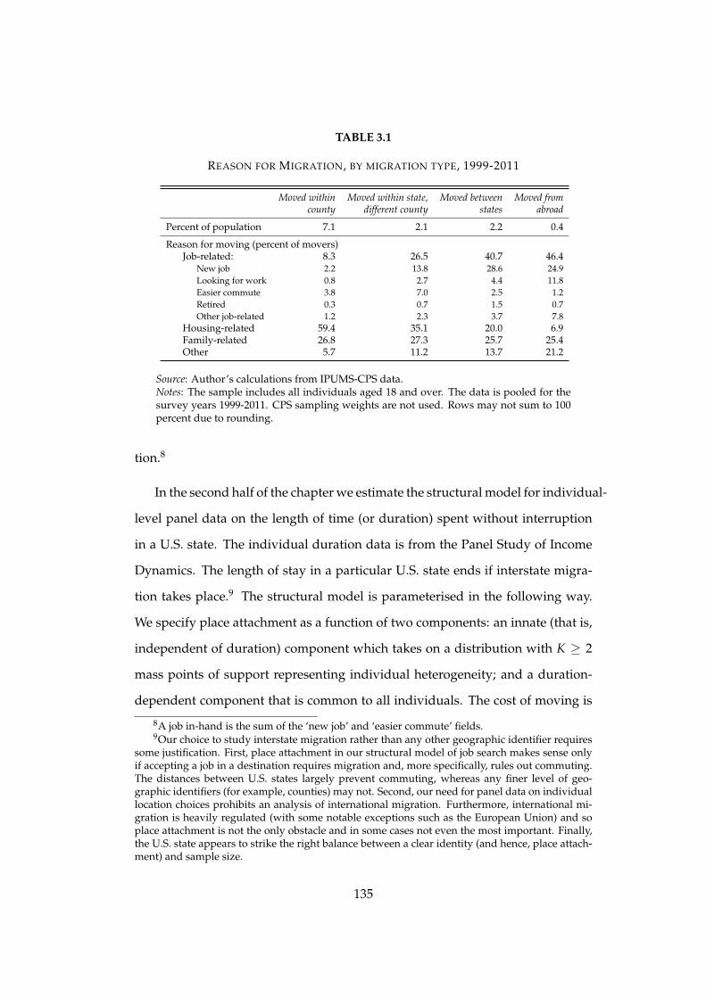
TABLE 3.1

REASON FOR MIGRATION, BY MIGRATION TYPE, 1999-2011

Moved within Moved within state, Moved between Moved fromcounty different county states abroad

Percent of population 7.1 2.1 2.2 0.4

Reason for moving (percent of movers)Job-related: 8.3 26.5 40.7 46.4

New job 2.2 13.8 28.6 24.9Looking for work 0.8 2.7 4.4 11.8Easier commute 3.8 7.0 2.5 1.2Retired 0.3 0.7 1.5 0.7Other job-related 1.2 2.3 3.7 7.8

Housing-related 59.4 35.1 20.0 6.9Family-related 26.8 27.3 25.7 25.4Other 5.7 11.2 13.7 21.2

Source: Author’s calculations from IPUMS-CPS data.Notes: The sample includes all individuals aged 18 and over. The data is pooled for thesurvey years 1999-2011. CPS sampling weights are not used. Rows may not sum to 100percent due to rounding.

tion.8

In the second half of the chapter we estimate the structural model for individual-

level panel data on the length of time (or duration) spent without interruption

in a U.S. state. The individual duration data is from the Panel Study of Income

Dynamics. The length of stay in a particular U.S. state ends if interstate migra-

tion takes place.9 The structural model is parameterised in the following way.

We specify place attachment as a function of two components: an innate (that is,

independent of duration) component which takes on a distribution with K ≥ 2

mass points of support representing individual heterogeneity; and a duration-

dependent component that is common to all individuals. The cost of moving is

8A job in-hand is the sum of the ‘new job’ and ‘easier commute’ fields.9Our choice to study interstate migration rather than any other geographic identifier requires

some justification. First, place attachment in our structural model of job search makes sense onlyif accepting a job in a destination requires migration and, more specifically, rules out commuting.The distances between U.S. states largely prevent commuting, whereas any finer level of geo-graphic identifiers (for example, counties) may not. Second, our need for panel data on individuallocation choices prohibits an analysis of international migration. Furthermore, international mi-gration is heavily regulated (with some notable exceptions such as the European Union) and soplace attachment is not the only obstacle and in some cases not even the most important. Finally,the U.S. state appears to strike the right balance between a clear identity (and hence, place attach-ment) and sample size.

135

assumed to be a function of a constant term and the distance-to-destination.

Paying close attention to how our sample is generated, we estimate the search

model for the unknown parameters of interest using maximum likelihood. In

order to mitigate omitted variable bias, we control for a number of variables that

have been found to affect migration in the literature, including age, gender, race,

marital status and education. The estimation is a nested problem: the inner loop

of the optimisation routine solves – for given parameter values – the differential

equation for the reservation income; the outer loop uses the reservation income

to compute the likelihood of observing our sample of durations and updates the

parameter values. The algorithm stops when the likelihood of observing the data

is maximised.

The structural approach to estimating place attachment has a number of ben-

efits. First, the estimates are grounded in economic search theory, of which one

of the key insights is that the current reservation value for migration is directly

influenced by future values of the reservation value. For example, if place at-

tachment is expected to rise with duration spent in the current state, then this

will increase the future reservation value and, in turn, the current reservation

value for migration. Second, in the structural model place attachment is mea-

sured in the same units as income. This helps with interpreting the parameter

estimates because they are income-equivalent. For comparison, we also present

reduced-form estimates.

Our results are rather surprising. While our reduced-form estimates suggest

that place attachment is increasing in the length of stay in a U.S. state, our struc-

tural estimates suggest the opposite. Furthermore, this is true for both the sample

of individuals that reside in the state they grew-up in as well as the sample of in-

dividuals that live in a state other than the one they grew-up in. More research

is needed to verify whether the structural estimates can be relied upon.

136

This chapter is most closely related to the literature on job search and mi-

gration. The findings from early studies of spatial job search are that personal

unemployment significantly increases the probability of outmigration and, in

addition, there is some evidence to suggest regional unemployment encourages

outmigration too (see Herzog Jr et al. (1993) for a survey). Rogerson and MacKin-

non (1981), Pickles and Rogerson (1984) and McCall and McCall (1987) were the

first papers to apply formal job search theory to the study of migration.10 These

papers assume a stationary wage offer distribution in a destination, whereas we

allow this to vary over time. Moreover, they do not estimate their models. Ken-

nan and Walker (2003) is similar to our work in the sense that their focus is on the

estimation of a structural model of migration where the incentive for migration

is expected income. However, they are interested in quantitatively showing that

regional income differentials matter for migration decisions, which they find is

the case. In contrast, we are concerned with estimating place attachment.11,12

This chapter is also related to the huge literature on the theory and estimation

of job search models.13 Finally, our work also belongs to the literature on the

estimation of dynamic structural discrete choice models.14

The remainder of the chapter is organised as follows. In section 3.2 we present

a sequential search model of migration choice under uncertainty. The section

10For other related theoretical contributions see Miron (1978) for an early attempt to apply jobsearch theory to migration; Coulson et al. (2001) who study job search for rural-urban migrationwhen commuting is permitted; and Ortega (2000) who uses a job search framework to identify amechanism through which natives gain from immigration.

11Kennan and Walker (2003) assume migration precedes job search. We, however, assume thatjob search precedes migration. Also their methodology is different. They estimate a dynamicdiscrete choice model via solving the dynamic programming problem directly with the computer.In order to do this for 5o U.S. states they have to heavily discretise the wage distribution, whichwe do not.

12See also Topel (1986), Fahr and Sunde (2002) and Basker (2003) for empirical studies of jobsearch and migration.

13See Lippman and McCall (1976) and Rogerson et al. (2005) for surveys of job search and, forthe estimation of search models using duration of unemployment data, see Lancaster (1979), Flinnand Heckman (1982), Van Den Berg (1990).

14See Eckstein and Wolpin (1989), Rust (1994), Keane and Wolpin (2009) and Aguirregabiriaand Mira (2010) for excellent surveys.

137

culminates in a structural equation for the migration (or hazard) rate and its as-

sociated distribution for length of stay (or duration) as a function of place attach-

ment, personal circumstances and regional labour market conditions. Section 3.3

describes the data, details the estimation of the model and explains the results.

Finally Section 3.4 concludes.

3.2 The Model

The model has its foundations in job search theory. Time is continuous and in-

dexed by t. We define a ‘spell’ for an individual to be the time during which he

or she is continuously resident in a particular region.15 We use ‘spell duration’

to refer to the length of time spent in a spell. For ease of exposition we assume

the spell start date is t = 1 such that time and spell duration coincide.16 Individ-

uals work until (exogenous) time T < ∞, at which point the individual retires

yielding zero utility.17 Individuals are subject to a possibility of death that fol-

lows a Poisson process with death rate parameter φ.18 The economy consists of

J + 1 < ∞ regions indexed by j.

Individuals inelastically supply one unit of labour in a short time interval δt

in return for income. Let i denote the current region. At time t an individual in

region i has (labour) income yit ≥ 0. This income evolves over time in response to

changing labour market conditions in region i and individual circumstances. We

take the evolution of individual income in region i as exogenous.19 In addition,

15Hence, migration from the source region and subsequent return migration to the source aretreated as two distinct spells in the source.

16Our working definition of a migrant is a person who changes his or her region of residencefor a period of at least a year; hence, a spell starts at d = 1.

17Therefore, we do not consider the migration choices of retired individuals.18Therefore, in a small time interval δt, the probability of death is φδt. Death yields zero utility.19In other words, we do not allow the individual to have any influence on his income in region

i. If, for example, an individual is observed changing jobs within region i then this is assumedto be down to nature and not the result of an additional optimality condition by the individual.Although job search within a region is clearly important, we justify its omission here through our

138

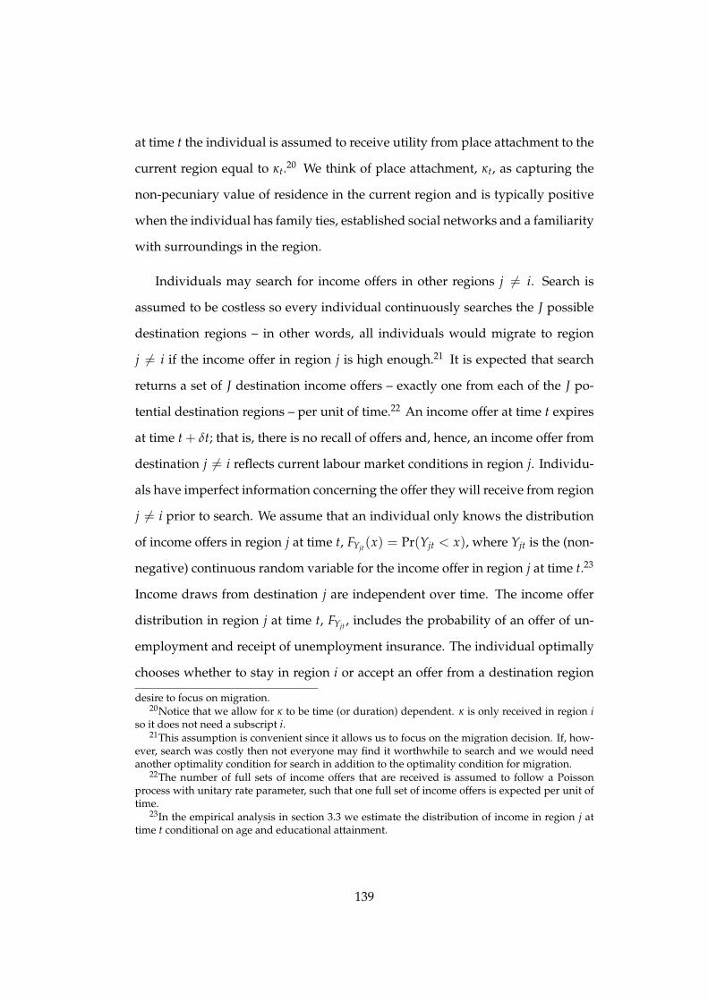
at time t the individual is assumed to receive utility from place attachment to the

current region equal to κt.20 We think of place attachment, κt, as capturing the

non-pecuniary value of residence in the current region and is typically positive

when the individual has family ties, established social networks and a familiarity

with surroundings in the region.

Individuals may search for income offers in other regions j 6= i. Search is

assumed to be costless so every individual continuously searches the J possible

destination regions – in other words, all individuals would migrate to region

j 6= i if the income offer in region j is high enough.21 It is expected that search

returns a set of J destination income offers – exactly one from each of the J po-

tential destination regions – per unit of time.22 An income offer at time t expires

at time t + δt; that is, there is no recall of offers and, hence, an income offer from

destination j 6= i reflects current labour market conditions in region j. Individu-

als have imperfect information concerning the offer they will receive from region

j 6= i prior to search. We assume that an individual only knows the distribution

of income offers in region j at time t, FYjt(x) = Pr(Yjt < x), where Yjt is the (non-

negative) continuous random variable for the income offer in region j at time t.23

Income draws from destination j are independent over time. The income offer

distribution in region j at time t, FYjt , includes the probability of an offer of un-

employment and receipt of unemployment insurance. The individual optimally

chooses whether to stay in region i or accept an offer from a destination region

desire to focus on migration.20Notice that we allow for κ to be time (or duration) dependent. κ is only received in region i

so it does not need a subscript i.21This assumption is convenient since it allows us to focus on the migration decision. If, how-

ever, search was costly then not everyone may find it worthwhile to search and we would needanother optimality condition for search in addition to the optimality condition for migration.

22The number of full sets of income offers that are received is assumed to follow a Poissonprocess with unitary rate parameter, such that one full set of income offers is expected per unit oftime.

23In the empirical analysis in section 3.3 we estimate the distribution of income in region j attime t conditional on age and educational attainment.

139

j 6= i and, if the latter, chooses among destination offers.24 Migration occurs if

the individual accepts an income offer from any destination j 6= i.

Let Vit denote the present discounted value of being resident in region i at

time t, and Vijt the random variable for the present discounted value of migration

from region i to region j at time t.25 Individuals take as given the time paths of the

key exogenous variables {yit, κt, FYjt ; ∀t, j 6= i}; or, alternatively, the individual

is assumed to correctly predict the future values of these exogenous variables.

In a short time interval δt, an individual in region i at time t with income yit

receives utility (yit + κt)δt.26 With probability (1− φδt) the individual survives

to time t + δt where, with probability 1.δt, the individual chooses to either accept

or reject the highest destination offer and, with probability (1− 1.δt), no set of

offers arrive. Therefore, the value of being resident in region i at time t is given

by the Bellman equation

Vit = (yit + κt)δt +(1− φδt)(1 + rδt)

[δtE max

{max

j 6=i{Vij,t+δt}, Vi,t+δt

}

+ (1− δt)Vi,t+δt

], (3.1)

where r > 0 is the rate of time preference and E is the mathematical expectation.

Multiplying by 1+rδtδt and taking the limit as δt tends to zero yields

(r + φ)Vit = yit + κt + E max{

maxj 6=i{Vijt} −Vit, 0

}+ Vit, (3.2)

where Vit ≡ ∂Vit∂t .

24That is, the regions are mutually exclusive.25Vijt is a random variable because it will be a function of the income offer distribution in

destination j from which the individual draws.26The assumption that utility is linear in income y and place attachment κ requires some ex-

planation. Assuming there exists complete (Arrow-Debreu) markets, maximising utility – for arisk-averse individual – is equivalent to maximising the sum of income and place attachment andthen smoothing per-period utility.

140

3.2.1 The Migration Decision

Now consider the individual’s choice whether to migrate or not at time t. To this

end, we need to write the value of migration from region i to j at time t, Vijt. We

assume a fraction cij > 0 of the income offer in destination j covers the (distance-

dependent) moving costs from region i to j.27 In the empirical section, cij will be

a function of the distance between i and j.28 Finally, we assume that migration is

an absorbing state; that is, there is no opportunity to move again post-migration

from region i.29 Then,

Vijt =Yjt

Rjt− cijYjt

≡Yjt

Rjtcijt, (3.3)

27Note that cij does not include the cost of relinquishing place attachment, which is captured byκ. A moving cost that is proportional to the income offer helps with tractability; more specifically, ityields a closed-form solution for the probability of choosing destination j conditional on migration(see equation 3.10). Its analogy in trade theory is an iceberg cost of moving goods between tradepartners. However, in our migration context (and since later we will take the model to the data) itneeds some justification why moving costs are proportional to the income offer. The assumptionrequires two leaps of faith. First, for a given individual, regions with (on average) lower incomeoffers also have lower moving costs – holding distance constant. In support of this one may arguealong the lines of different regional price levels (although, if so, then clearly it would be better tomake cij a function of the price level in destination j instead of assuming proportionality to theincome offer). Second, within a destination region, a person that draws a low income offer has alower cost of moving than an otherwise identical person that draws a high income offer. One mayargue that high earners tend to spend more on moving but then one may expect them to yieldsome utility from this higher expenditure. Nonetheless, among others Borjas (1987) makes theassumption that migration costs are proportional to income.

28We could allow cij to be individual-specific. In particular, we could control for whether theindividual owned his or her own house in region i as well as controlling for individual-specific in-formation frictions. Information frictions may be eased by social networks (for example, relativesresiding in destination j) and whether the individual has previously resided in the region. Ourempirical estimation could be extended in this direction.

29This additional assumption is perhaps not as restrictive as first may seem. In the empiricalsection, at time t, future income in current region i is forecast out to age 64 conditional on individ-ual experience and education. Conditional on migration to destination j, the future income streamin destination j is forecast out to age 64 by applying the (region-specific) growth rate and return toexperience to the income draw at time t. Any subsequent migration due to unforecastable eventswill not affect the migration decision at time t. We should, however, be concerned about the effectof additional migration beyond time t on the value of migration at time t that is both forecastableand not captured by the region-specific return to experience.

141

where 1/Rjt ≡∫ T

t e−(r+φ−gjt)(τ−t)dτ =1−exp[−(r+φ−gjt)(T−t)]

r+φ−gjtis the expected present

discounted value of one dollar of income in destination j at time t; gjt is the ex-

pected (constant) growth rate of income in destination j from time t to time T

(which combines the effects of regional growth and the regional return to expe-

rience); and cijt ≡ 11−cijRjt

. Notice that the present value factor 1/Rjt captures

precisely the human capital theory explanation for why migration rates fall with

age; that is, the young experience a longer period of returns from migration and

the one-off moving costs are spread over a larger number of years (Becker, 1964).

In deciding whether to migrate or not, the individual only considers the high-

est present value income offer – net of the cost of moving – from the set of J des-

tination offers. Let Vi−,t ≡ maxj 6=i{Vijt} denote the random variable for the max-

imum present value income offer. Since the value of migration to region j, Vijt,

is increasing in the income offer in region j, and staying an additional instant of

time in region i at time t, Vit, is independent of the income draw in region j, the

solution to the individual maximisation problem is a unique reservation value

for Vi−,t, call it v∗i−,t, satisfying

v∗i−,t = Vit,

such that the individual migrates from region i if she receives an income offer

with present value that exceeds v∗i−,t and stays in region i otherwise. Substituting

this reservation value into equation (3.2) yields the following non-linear first-

order differential equation for the reservation value (or present value of income

net of moving cost) at time t,30

∂v∗i−,t

∂t= (r + φ)v∗i−,t − yit − κt − E max

{max

j 6=i

{Yjt

Rjtcijt

}− v∗i−,t, 0

}, (3.4)

30See Van Den Berg (1990) for a proof that this non-stationary case has a unique solution for thereservation value.

142

where recall that Yjt is the random variable for the income offer in region j at time

t.

3.2.2 The Choice Between Destinations

The random variable for the value of migration from region i to region j at time

t, Vijt, has distribution function

FVijt(v) ≡ Pr(Vijt ≤ v)

= Pr(Yjt ≤ vRjtcijt)

= FYjt(vRjtcijt). (3.5)

The maximum offer value Vi−,t has distribution function

FVi−,t(v) = 1− Pr(Vi−,t > v)

= 1− [1−∏j 6=i

FVijt(v)], (3.6)

where the second equality uses the fact that Pr(Vi−,t > v) is one minus the prob-

ability that all {Vijt; j 6= i} are less than or equal to v and {Yjt; j = 1, ..., J} are

assumed independent across j for all t. It is common to assume that the dis-

tribution of income in region j at time t, FYjt , is Lognormal. However, under a

Lognormal distribution the expression for FVi−,t is complicated. There is, how-

ever, a distribution for Yjt that leads to a tractable expression: the Frechet (or

type II extreme value) distribution,

FYjt(x) = exp(−Ajtx−α), (3.7)

143

where Ajt > 0 is a location parameter specific to region j at time t and α > 1

is a shape parameter common to all regions.31,32 Since ultimately we will take

the model to the data, the reader may be worried about the appropriateness of

the Frechet distribution for income. Figure 3.1 plots the Frechet density (dashed

line) and the Lognormal density (solid line) for two different sets of parame-

ter values.33 Casual eye-balling of the two densities reveals that they look very

similar – both are bell-shaped. The main difference is that the Frechet has a fat-

ter right-tail than the lognormal, but they are close.34 Moreover, it is unclear

how much individuals know or care about the tail of the distribution – perhaps

the tails need to be fat but their precise shape may not be important. Figure

3.2 plots synthetic data drawn from a Frechet distribution and fits a Lognormal

to the synthetic Frechet, first by maximum likelihood and then by minimising

the Kolmogorov-Smirnov statistic.35 Both the fitted Lognormal distributions are

close to the Frechet and, minimising the Kolmogorov-Smirnov statistic provides

31Note the support of the distribution is [0, ∞). We restrict α to be greater than one so that thefirst moment is finite. The expectation is,

E(Yjt) =∫ ∞

0xαAjtx−α−1 exp(−Ajtx−α)dx

= A1/αjt

∫ ∞

0z−1/α exp(−z)dz

= A1/αjt Γ

(α− 1

α

), (3.8)

where Γ is the Gamma function Γ(x) =∫ ∞

0 ux−1 exp(−u)du. Recall α > 1, hence α−1α ∈ (0, 1).

Note limα→∞ Γ(

α−1α

)= 1 and limα→1 Γ

(α−1

α

)= ∞. Clearly the expected income is increasing in

Aj.32Only the Frechet distribution leads to an extreme value distribution for the value of migration

to the best alternative region (see Eaton and Kortum (2002) for an analogous use of the Frechetdistribution in the trade of goods).

33Both distributions have two parameters: a location and scale parameter. To construct Figure3.1, we first fitted a Frechet to a simulated Lognormal by maximum likelihood; however, maxi-mum likelihood tended to be sensitive to the tails and so visually it did not give a good fit. In theend we simply chose parameter values by trial and error using the graphs and our eyes to judge.

34Kleiber and Kotz (2003) survey the literature on the distribution of income and find thatalthough there is some evidence in support of log-normality, it is by no means perfect and in somecases other distributions achieve a better fit. However, the Frechet is not considered.

35Minimising the Kolmogorov-Smirnov statistic for fitting an empirical distribution to a theo-retical one is arguably better (for our purposes) than maximum likelihood because Kolmogorov-Smirnov looks at the difference between the cumulative distribution functions and as such ‘over-fits’ the middle of the distribution. We discuss this issue in the empirical section.

144

a better visual fit than maximum likelihood since the former ‘over-fits’ the mid-

dle of the distribution.

FIGURE 3.1

DENSITY OF A FRECHET AND LOGNORMALDISTRIBUTION

FIGURE 3.2

FITTING A LOGNORMAL TO A FRECHET: MAXIMUM LIKELIHOOD VERSUSKOLMOGOROV-SMIRNOV DISTANCE MINIMISATION

a) PLOT OF CDF b) PLOT OF PDF

Using (3.5), (3.6) and (3.7), we get the following neat expression for FVi−,t ,

FVi−,t(v) = exp

(−∑

j 6=iAjt(vRjtcijt)

−α

). (3.9)

145

As the cost of migration (cijt) tends to infinity for all j, the probability of migration

tends to zero.36 Conditional on exit from region i at time t, the probability of

choosing destination region j is

pijt = Pr[Vijt > max{Vimt; ∀m 6= i, j}]

=∫ ∞

0∏

m 6=i,jFVimt(v)dFVijt(v)

= Ajt(Rjtcijt)−α∫ ∞

0exp

[− ∑

m 6=iAmt(vRmtcimt)

−α

]αv−α−1dv

=Ajt(Rjtcijt)

−α

∑m 6=i Amt(Rmtcimt)−α

∫ ∞

0

ddv

exp

[− ∑

m 6=iAmt(vRmtcimt)

−α

]dv

=Ajt(Rjtcijt)

−α

∑m 6=i Amt(Rmtcimt)−α, (3.10)

where the second equality is by independence and the third equality substitutes

the expression for FVijt from equation (3.5).

3.2.3 The Reservation Value

Using the derived distribution of the maximum in (3.9), the reservation value in

equation (3.4) can be written as

∂v∗i−,t

∂t= (r + φ)v∗i−,t − yit − κt −

∫ ∞

v∗i−,t

[v− v∗i−,t]dFVi−,t(v). (3.11)

36The expected value of migration from region i at time t is

E(Vi−,t) =

∑j 6=i

Ajt(Rjtcijt)−α

1/α

Γ(

α− 1α

).

146

The integral on the right-hand-side of (3.11) can be expressed as

∫ ∞

v∗i−,t

[v− v∗i−,t]dFVi−,t(v) =

[∑j 6=i

Ajt(Rjtcijt)−α

]1/α

×

× γ

(α− 1

α, ∑

j 6=iAjt(v∗i−,tRjtcijt)

−α

)

− v∗i−,t[1− FVi−,t(v∗i−,t)],

where γ(s, x) =∫ x

0 ts−1e−tdt is the lower incomplete gamma function.

The key exogenous variables in the model – income in the current region, yit,

place attachment κt and the distribution of income offers in region j 6= i, Fjt(x) –

are all time (or duration) dependent. Therefore, the reservation value – given by

the non-linear first-order differential equation in (3.11) – is also time dependent.

At time t the individual makes forecasts for these exogenous variables over his

remaining working life (T − t). At time T (retirement age 65) we impose the

boundary condition ViT = 0. Most importantly, at time t, individual expectations

of the future impact on the reservation value at time t. For example, if place

attachment, κt, is expected to increase with duration beyond time t, then this will

increase the reservation value at time t all else equal. Using numerical methods,

the differential equation in (3.11) can be solved recursively from time t = T for

the reservation value v∗i−,t.

3.2.4 The Conditional Migration Rate and Distribution of Duration

In section 3.3 we will estimate our structural model of migration for a sample of

individual spell durations. Before we do this, we need to derive the implied mi-

gration (or hazard) rate conditional on duration and – in turn – the correspond-

ing distribution for spell duration. Define hij(t) as the migration (or hazard) rate

from region i to region j at time t, conditional on spending at least t periods in

147

region i. Given the reservation value at time t, v∗i−,t, the destination-j hazard rate

is

hij(t) = pijt[1− FVi−,t(v∗i−,t)]. (3.12)

Let Dij denote the continuous random variable for duration in region i if it were

only possible to migrate to destination j. It has the well-known distribution func-

tion

FDij(d) = 1− exp(−∫ d

0hij(z)dz

), (3.13)

which is the foundation of the maximum likelihood estimation in the next sec-

tion. The overall hazard rate for migration from region i at time t to any desti-

nation j 6= i is simply the sum of the destination-specific hazard rates (they are

mutually exclusive events)

hi(t) = ∑j 6=i

hij(t) = [1− FVi−,t(v∗i−,t)]. (3.14)

Let Di denote the continuous random variable for spell duration in region i. It

has the distribution function

FDi(d) = 1− exp(−∫ d

0hi(u)du

). (3.15)

3.3 Empirical Analysis

We now estimate the above search model using panel data on individual inter-

state migration in the United States (U.S.). The theory outlined above yields

an expression for the migration (or hazard) rate to destination j and, hence, the

probability distribution of spell duration. Our sample of individual spell du-

148

rations in U.S. states comes from the University of Michigan’s Panel Study of

Income Dynamics (PSID). We maximise the likelihood of observing our sample

while imposing the restrictions implied by the structural model. In doing so, we

pay careful attention to the specific way our duration sample was generated.37

For comparison with the structural model, we present reduced-form estimates

of the unknown parameters. In what follows we describe the data, outline the

empirical strategy and present the results of the estimation for the unknown pa-

rameters of interest.

3.3.1 The Data

Recall that to test the theory we require data on the following variables: spell du-

ration, d; individual income in the current region i at time t, yit; place attachment

at time t, κit; the distribution of income offers in state j at time t, FYjt ; and the cost

of migration from region i to j, cij. Here we discuss the source of the data (see

Appendix 3.A for a description of each variable used in the analysis).

Our data on individual location choices comes from the PSID. The PSID is a

longitudinal survey that follows 4,802 original families (and all their subsequent

split-offs) residing in the U.S. annually from 1968 to 1997 and biennially from

1997 to 2009.38 At the time of the most recent survey in 2009, the PSID followed

37See Jenkins (2005) for an introductory survey on the techniques of duration analysis.38This includes the 1,872 low-income families in the Survey of Economic Opportunity (SEO)

subsample. We apply the PSID sampling weights to make our estimates representative of the U.S.population. Becketti et al. (1988) compares the empirical distributions of cross-sections of the PSIDwith the large-sample Current Population Survey (CPS) for a number of demographics includingage, sex, race, years of education, labour income, marital status, census region and employmentstatus. These authors also looked at various subsamples including heads of households, which isour unit of analysis. The authors found that – once the sampling weights are accounted for – thedifferences between the PSID and CPS are negligible. Looking at the more recent period 1993-2005,Gouskova et al. (2008) also finds that the differences between the weighted distributions of thePSID and CPS are small (with the possible exception of race). Thus it seems that – despite the initialover-sampling of low-income (and black) SEO families, differential attrition across survey waves(the longitudinal PSID suffers from non-response and mortality) and an increase in the proportionof young families in later waves (due to split-offs) in the PSID sample – the PSID sample remainsrepresentative of the U.S. population once the sampling weights are applied. The PSID individual

149

8,690 families. Importantly for our purposes, the study records the U.S. state of

residence for an individual in each survey year and from this we compute (in-

sample) duration in a particular state, which constitutes our measure of d.39,40 A

‘region’ in the above theoretical model now refers to a U.S. state and migration

(or hazard) pertains to interstate migration.

The PSID also contains detailed information on the personal circumstances of

the respondents in each survey year, including income. We measure yit as pre-tax

labour income; that is, the sum of wages, bonuses and the amount of business

income attributable to labour. We express income in constant 1999 dollars using

the U.S. Consumer Price Index for all urban consumers (CPI-U). The PSID also

records age, gender, race, marital status and education, which serve as controls

in the maximum likelihood estimation.

The distribution of income offers for an individual in potential destination

state j at time t, FYjt , is assumed to be given by the empirical distribution of in-

come in state j at time t. We use the March Supplement of the Current Population

Survey (CPS), 1968-2011, to estimate the empirical income distribution for each

state-year.41,42 In addition to income, the CPS records the individual’s state of

residence, age and education. We fit the Frechet distribution – separately for each

sampling weights are updated over successive survey waves precisely to account for differentialattrition. Non-sample persons (individuals who enter the sample through marriage or living witha sample person) are assigned a zero weight. Non-sample persons are much more likely to leavethe sample – the PSID does not follow non-sample persons when they leave a sample household.

39We assume it is infeasible to migrate interstate more than once within a two-year time spanand, hence, we can track duration over this 42-year period. This is consistent with the UnitedNation’s definition of migration based on length of stay, which requires a change in the place ofprimary residence for a period of at least a year. People moving for shorter durations are termedvisitors, not migrants. Nonetheless, the results do not significantly change if we drop the biennialobservations.

40The PSID is the longest running panel dataset and, hence, is particularly suited to our dura-tion analysis where we must track individuals sequentially. We are able to follow some individualsfor 42 years.

41We obtained the CPS data from the Minnesota Population Center’s Integrated Public UseMicrodata (see King et al. (2010)).

42We chose to use the CPS (rather than the PSID) to estimate the income distribution because ofits much larger sample. The geographic coverage of the CPS is the 50 U.S. states and the Districtof Columbia, which coincides with the coverage of the PSID.

150

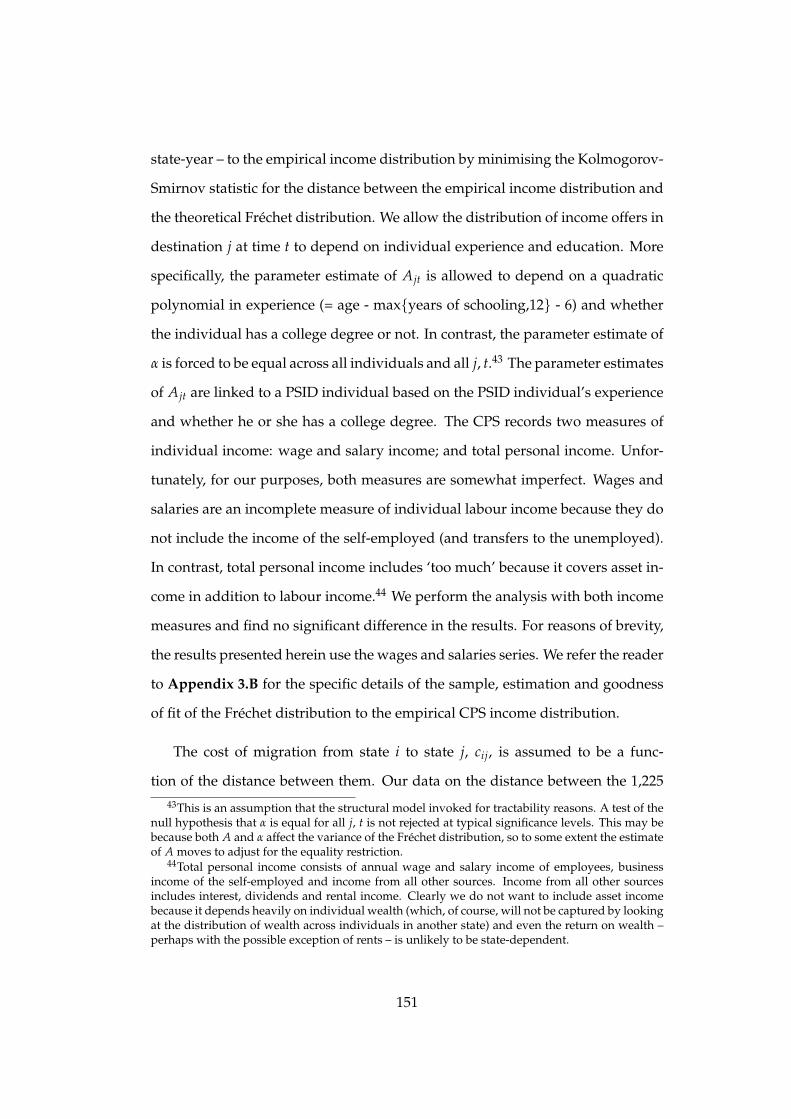
state-year – to the empirical income distribution by minimising the Kolmogorov-

Smirnov statistic for the distance between the empirical income distribution and

the theoretical Frechet distribution. We allow the distribution of income offers in

destination j at time t to depend on individual experience and education. More

specifically, the parameter estimate of Ajt is allowed to depend on a quadratic

polynomial in experience (= age - max{years of schooling,12} - 6) and whether

the individual has a college degree or not. In contrast, the parameter estimate of

α is forced to be equal across all individuals and all j, t.43 The parameter estimates

of Ajt are linked to a PSID individual based on the PSID individual’s experience

and whether he or she has a college degree. The CPS records two measures of

individual income: wage and salary income; and total personal income. Unfor-

tunately, for our purposes, both measures are somewhat imperfect. Wages and

salaries are an incomplete measure of individual labour income because they do

not include the income of the self-employed (and transfers to the unemployed).

In contrast, total personal income includes ‘too much’ because it covers asset in-

come in addition to labour income.44 We perform the analysis with both income

measures and find no significant difference in the results. For reasons of brevity,

the results presented herein use the wages and salaries series. We refer the reader

to Appendix 3.B for the specific details of the sample, estimation and goodness

of fit of the Frechet distribution to the empirical CPS income distribution.

The cost of migration from state i to state j, cij, is assumed to be a func-

tion of the distance between them. Our data on the distance between the 1,22543This is an assumption that the structural model invoked for tractability reasons. A test of the

null hypothesis that α is equal for all j, t is not rejected at typical significance levels. This may bebecause both A and α affect the variance of the Frechet distribution, so to some extent the estimateof A moves to adjust for the equality restriction.

44Total personal income consists of annual wage and salary income of employees, businessincome of the self-employed and income from all other sources. Income from all other sourcesincludes interest, dividends and rental income. Clearly we do not want to include asset incomebecause it depends heavily on individual wealth (which, of course, will not be captured by lookingat the distribution of wealth across individuals in another state) and even the return on wealth –perhaps with the possible exception of rents – is unlikely to be state-dependent.

151

(= 50(50− 1)/2) pairs of states comes from Google Maps and is measured as the

crow flies in kilometres. Finally, place attachment at duration d, κ(d), is unob-

servable. We will specify later how it is parameterised.

3.3.2 Descriptive Statistics

Our PSID sample of duration spells suffer from three forms of censoring. First,

interval-censoring occurs when the spell start date is known and the end date is

known to lie within an interval. Recall the structural model presented in section

3.2 assumed duration choice is a continuous process; that is, an individual can

choose to migrate from the current state of residence at any point in continuous

time. In contrast, in our PSID sample we only observe an individual’s state of

residence at the time of interview. Therefore, our duration data is intrinsically

grouped (or interval-censored). In our sample, a spell is interval-censored when

an individual is followed regularly (at least biennially) from the spell start date

until, between two interviews one or more years apart, the individual is recorded

as migrating from the state.45 The start date of a spell is assumed known if an

individual is followed from age 17 or it is a spell commencing immediately (two

years or less) post-migration.46 Interval-censored spells represent the most de-

tailed data we have on spell duration.

Second, right-censoring occurs when we do not observe the end date of a

duration spell. This happens either when an individual attrits from the sample

(due to non-response or mortality) or their spell remains incomplete at the time

of the 2009 PSID survey – the last available.47 Attrition is unlikely to be random.

45The length of the interval at the time of censoring varies across spells due to the survey design(annual prior to 1997 and biennial since), non-response and missing values for the current statearound the time of migration and – because we will limit the analysis to heads of households –changes out of and into head status. Missing values are very rare.

46The PSID definition of where an individual grew up refers to ‘most of the years age 6 to 16’;so if we observe the state of an individual at age 17, we treat this as the spell start date.

47The 1968-2009 PSID Death File records the precise year of death if known. Therefore, we use

152

For our purposes this is only a concern if attrition is related to the determinants of

spell duration.48 The individuals that leave the survey represent a huge amount

of data and, in many cases, have a long stream of continuous response prior to

exit that we do not want to discard. Becketti et al. (1988) found that attrition

in the PSID due to non-response is much higher in the first year of entry but

shows no subsequent duration dependence. We take this seriously and drop all

individuals that respond to just a single survey.49,50 If spell i is right-censored

then we know that duration exceeds some level.

Third, and finally, left-censoring is when we do not know the start date of the

duration spell. Predominantly this occurs when an individual enters the sample

above age 17 since we do not know the migration history of individuals at entry.

Hence, with left-censored spells we simply do not know duration at any point

during the spell. This is problematic for our analysis because place attachment,

κ(d), is a function of duration. Therefore, in addition to the full sample, we

present the results for the subsample that drops left-censored spells.

When there is a gap between state records of more than two years, we split

the spell into two, imposing right-censoring on the spell prior to the split and

left-censoring on the spell after.51 In our data, all spells are censored and some

this information rather than the survey year when the gap between interviews is more than a year.48In theory one could model the attrition process as a function of spell duration and solve for

spell duration as the solution to two simultaneous equations. This is, however, a considerablecomplication in a model that is already computationally demanding.

49Individuals that respond to just a single survey fall out of the sample anyway when we laglabour income to reflect the fact that respondents are asked about their income in the previousyear.

50In other, less supportive evidence, Zabel (1998) finds that the chances of attrition in the PSIDare related to sample duration (although weaker than in the SIPP) and mobility. If – despite theexhaustive efforts of PSID staff to follow sample members – individuals are more likely to dropout of the sample post-migration then this is a concern.

51As already mentioned, due to missing observations and changes out of and into Head status,the length of the interval between state records varies. When no change in state is recorded withinan interval of more than two years then we cannot be sure that migration did not take place duringthis period. If instead we observe that migration did take place, then admittedly it is less clear thatone would want to censor this. Clearly the larger the interval the less information it conveys,particularly when we consider time-varying covariates later (the maximum likelihood estimationwill assume covariates are constant within the interval and, naturally, the longer the interval the

153

are doubly censored in the sense that they are left- and right-censored.52 In what

follows, we refer to left and right-censored spells simply as censored spells when

the distinction is not important; that is, when we only use the information that

in both cases duration exceeds some level. Interval-censored spells – which con-

tain more precise information on duration – are referred to explicitly as interval-

censored.53

We restrict the PSID sample to heads of households since we feel that – of all

family members – the head is most likely to make migration decisions.54 Since

our model of migration is based on job search, we drop those observations when

an individual is aged 65 or over. This leaves us with data on 19,712 spells by

13,481 individuals. Of these, 1,568 spells (or 8 percent) are interval-censored and

the vast majority (16,065 or 81 percent) are left-censored. On average – combining

interval-censored and censored spells – duration in a state is roughly 7 years.

Nearly 40 percent of spells are in a host state (that is, a state other than the state

the individual grew up in) and 81 percent of our interval-censored spells are in a

host state.

Table 3.2 presents the empirical frequency distribution of duration in our

sample. The second column of the table lists the number of spells – interval-

censored and censored combined – by spell duration. Almost 24 percent of spells

last just a year, 51.7 percent four years or less and 77.4 percent ten years or less.

Generally speaking then, the number of spells fall exponentially with duration.

less likely this assumption is reasonable). For this reason, we chose to impose right-censoring onthe few cases where the interval-censoring is more than two years.

52To be clear, interval-censored spells are – by definition – neither left nor right-censored.53The duration literature (on grouped-data) often refers to completed and incomplete spells for

interval-censored and right-censored spells, respectively. However, since some of our observa-tions are left-censored, a distinction based on completed and incomplete spells is not useful – acompleted spell can be left-censored.

54In reality migration is likely to be a joint decision between the head and “wife” (if present)but including both would be double-counting. Naturally a better model would treat the familyas the decision maker and optimise subject to the bargaining weights of each family member andtheir personal circumstances, which is beyond the scope of this chapter. Note that the PSID surveyrecords far more information about the head than any other family member.

154

Columns three to six document the number of spells that are interval-censored,

left-censored, in a host state and belong to an individual with multiple spells, re-

spectively. Interval-censored spells, host spells and multiple spells become much

less frequent as duration increases. This is to be expected given that these spells

are either likely to or have to involve migration and, hence, short spells. Just

over half of all spells are those of individuals with multiple spells, although the

number of individuals with multiple spells is substantially less than half.

Table 3.3 presents the frequency distribution of the number of spells per in-

dividual. Roughly 73 percent of individuals have just one spell and 89 percent

have two or fewer spells.55 The prevalence of multiple spells implies the need to

account for dependence across spell durations of the same individual.56

Table 3.4 lists the frequency distribution for the subsample that drops left-

censored spells. The sample size is substantially reduced to 3,647 spells and

the key (for identification) interval-censored spells make up 43 percent of these

spells. Compared to the full sample, in the subsample a much larger fraction

(70 percent) of spells take place in a host state and a much larger proportion (69

percent) are spells of individuals with multiple spells.

Our theory of duration laid out in Section 3.2 relates most closely to the haz-

ard function; that is, the probability of exiting a state conditional on duration.

The (Kaplan-Meier) empirical hazard rate (for the full sample) is shown in Fig-

ure 3.3.57 We grouped durations into two-year intervals to be consistent with the

highest interval length of our interval-censored observations. Let t index two-55On the one hand, because our sample does not follow individuals throughout their whole life

this table underestimates the number of spells per individual; on the other hand, the splitting ofspells where missing values occur overestimates the number of spells per individual.

56Although imperfect, we will cluster the standard errors at the individual level to allow thiswithin-individual, across-spell dependence to affect the precision of our parameter estimates.

57Note that there is no problem with including left-censored spells here since to compute theKaplan-Meier hazard we only need to know that duration exceeds some level for left-censoredobservations. Also note that the Kaplan-Meier estimates are non-parametric.

155

TABLE 3.2

DISTRIBUTION OF DURATION

Duration Frequency Frequency Frequency Frequency Frequency Percent Cumulativein Years All Spells Interval-censored Spells Left-censored Spells Host Spells Multiple Spells All Spells Percent

1 4,707 682 3,483 2,267 2,981 23.9 23.92 1,819 249 1,392 897 1,053 9.2 33.13 2,494 187 2,030 1,049 1,356 12.7 45.84 1,165 107 951 523 548 5.9 51.75 2,064 95 1,826 932 726 10.5 62.16 581 56 464 211 341 2.9 65.17 965 40 808 320 476 4.9 70.08 406 31 326 122 212 2.1 72.09 745 20 634 253 339 3.8 75.810 317 11 265 83 156 1.6 77.411 1,194 20 1,116 444 651 6.1 83.512 246 17 203 81 117 1.2 84.713 216 12 187 55 90 1.1 85.814 288 7 263 58 101 1.5 87.315 248 7 206 65 100 1.3 88.616 215 3 176 59 85 1.1 89.617 216 7 186 48 81 1.1 90.718 180 5 144 45 81 0.9 91.619 163 3 144 34 55 0.8 92.520 135 1 108 38 50 0.7 93.221 133 1 111 35 39 0.7 93.822 111 2 92 24 37 0.6 94.423 112 2 91 25 38 0.6 95.024 113 1 92 17 41 0.6 95.525 114 1 99 22 32 0.6 96.126 107 0 93 22 25 0.5 96.727 76 0 70 18 15 0.4 97.028 152 0 146 36 7 0.8 97.829 65 0 53 16 14 0.3 98.130 44 0 34 8 13 0.2 98.431 35 1 24 9 14 0.2 98.532 48 0 41 11 10 0.2 98.833 37 0 35 4 3 0.2 99.034 40 0 31 7 8 0.2 99.235 37 0 29 10 8 0.2 99.436 45 0 38 7 8 0.2 99.637 11 0 10 1 1 0.1 99.738 28 0 28 4 0 0.1 99.839 10 0 7 2 2 0.1 99.840 30 0 29 1 0 0.2 100.0Total 19,712 1,568 16,065 7,863 9,914 100.0

Note: The sample consists of interval-censored, left and right-censored durations of heads of house-holds. A host spell is defined as a spell that takes place in a state other than the state the individualgrew up. For 219 spells the state the individual grew up is unknown and so the numbers in col-umn 5 are out of a total of 19,493 spells. The column indicating multiple spells denotes spells ofindividuals for which we observe more than one spell.

156

TABLE 3.3

DISTRIBUTION OF THE NUMBER OF SPELLSPER INDIVIDUAL

Number of spells Frequency Percent Cumulativeper Individual Percent

1 9,798 72.7 72.72 2,242 16.6 89.33 846 6.3 95.64 313 2.3 97.95 150 1.1 99.06 71 0.5 99.57 36 0.3 99.88 18 0.1 99.99 4 0.0 100.010 1 0.0 100.011 2 0.0 100.0

Total 13,481 100.0

year intervals of time. Let nict denote the number of interval-censored spells in

interval t and nct the number of censored spells in interval t (that is, the lower

bound for duration of the censored spell falls within interval t). The hazard rate

in interval t is 58

h(t) =S(t)− S(t + 1)S(t) + S(t + 1)

,

where the survivor function S(t) = ∏tx=1

(1− nic

xnic

x2 +nc

x

). The hazard estimates

make an adjustment for censored observations because they only affect the num-

ber at risk of exit and not the number that actually exit in interval t. From Figure

3.3 we see that the two-year interval hazard declines exponentially with dura-

tion. The probability of exit is highest in the first two years yet is still only 1.2

percent.59

Figure 3.4 plots separately the hazard rates for two subgroups: spells where

58An adjustment is made to account for the (2-year) grouping of the data. The adjustment is

that those at risk of exiting in interval t is nct +

nict

2 because we assume half of the interval-censoredobservations have failed by the mid-point of the interval. Hence, strictly speaking, this is a life-table estimator (and not a Kaplan-Meier estimator).

59The hazard rate does not fall monotonically as duration increases; this lack of smoothness islikely due to the very low numbers of interval-censored spells at higher durations.

157

TABLE 3.4

DISTRIBUTION OF DURATION IN SUBSAMPLE THAT DROPS LEFT-CENSOREDSPELLS

Duration Frequency Frequency Frequency Frequency Percent Cumulativein Years All Spells Interval-censored Spells Host Spells Multiple Spells All Spells Percent

1 1,224 682 930 887 33.6 33.62 427 249 338 325 11.7 45.33 464 187 330 319 12.7 58.04 214 107 153 166 5.9 63.95 238 95 158 167 6.5 70.46 117 56 84 86 3.2 73.67 157 40 95 88 4.3 77.98 80 31 51 50 2.2 80.19 111 20 70 67 3.0 83.110 52 11 25 39 1.4 84.611 78 20 51 45 2.1 86.712 43 17 28 30 1.2 87.913 29 12 18 15 0.8 88.714 25 7 18 15 0.7 89.415 42 7 20 21 1.2 90.516 39 3 20 25 1.1 91.617 30 7 14 17 0.8 92.418 36 5 20 21 1.0 93.419 19 3 10 14 0.5 93.920 27 1 20 17 0.7 94.721 22 1 14 11 0.6 95.322 19 2 8 10 0.5 95.823 21 2 11 11 0.6 96.424 21 1 10 10 0.6 96.925 15 1 8 5 0.4 97.326 14 0 7 4 0.4 97.727 6 0 4 2 0.2 97.928 6 0 3 4 0.2 98.129 12 0 7 7 0.3 98.430 10 0 2 6 0.3 98.731 11 1 6 5 0.3 99.032 7 0 4 4 0.2 99.133 2 0 2 0 0.1 99.234 9 0 2 1 0.2 99.535 8 0 5 4 0.2 99.736 7 0 2 3 0.2 99.937 1 0 1 0 0.0 99.939 3 0 1 0 0.1 100.040 1 0 0 0 0.0 100.0Total 3,647 1,568 2,550 2,501 100.0

158

FIGURE 3.3

INTERVAL HAZARD RATE

Note: A bar represents the hazard rate for atwo-year interval of time.

FIGURE 3.4

HAZARD RATE FOR STATE GREW-UPAND HOST SUBGROUPS

Note: The line graph is drawn from the mid-points of the two-year intervals.

the individual resides in the state he or she grew-up and spells where the indi-

vidual resides in a host state. Again, for both subgroups, the hazard rate declines

as duration increases. The hazard rate is much higher for an individual in a host

state than the state he or she grew-up in. The difference between the two hazard

rates declines with duration.

It is well-known, however, that the time-dependence of the hazard function –

in our case downward sloping – may in fact reflect individual heterogeneity (se-

lection) – both observed and unobserved – rather than time-dependence (Gins-

berg, 1973, Lancaster, 1979, Elbers and Ridder, 1982, Heckman and Singer, 1984).

If individuals have individually constant (time-invariant) hazard rates but these

levels vary across individuals, then those with low exit rates will become more

prominent in the sample as duration increases and, hence, in aggregate this indi-

vidual heterogeneity looks like time-dependence when it is not. Without control-

ling for individual heterogeneity, time-dependence and individual heterogene-

ity are observationally equivalent (see Elbers and Ridder (1982), Heckman and

Singer (1984)). Furthermore, controlling for covariates is useful because, clearly,

we would like to know the reasons for changes in the hazard rate other than the

159

passage of time.

3.3.3 Empirical Model

As in the model of section 3.2, we use i to denote the current state such that i

indexes duration spells. To account for the grouped (or interval-censored) na-

ture of our duration data we need to introduce further notation. Let s index

the set of survey dates. We use s(i) to denote the survey when an individual

was last seen in spell i. Let di denote actual duration for spell i and dis denote

(in-sample) observed duration for spell i at survey s. Then, dis(i) is (in-sample)

observed duration when an individual was last seen in spell i. We use di,s(i)+1

to denote duration of spell i if the individual had continued the spell until the

next available survey following s(i). If duration for spell i is interval-censored

then {di,s(i) ≤ di < di,s(i)+1}. If spell i is left or right-censored then we know that

duration exceeds some level, {di > di,s(i)}.

We want to make use of all available information. If an individual migrates

in our sample then we know which state he or she has chosen to migrate to and

we want to account for this in our estimation.60 To this end, define χij to be an

indicator variable that takes the value one if the spell is interval-censored and

migration to region j is observed, and zero otherwise (exit to a state other than j

or censored). These are mutually exclusive events (death is treated as censored).

Although migration can occur to at most one destination at any one time,

with grouped data it is possible that, by the time of the next survey, other destination-

specific hazards may have been triggered. Therefore, in writing down the like-

lihood of observing an interval-censored duration and migration to destination

60The duration literature on this is called ‘competing risks’. Each individual has a latent haz-ard rate for migration to each state. We assume these latent hazard rates are independent, whichfollows from the assumption in the structural model that the income offer distributions are inde-pendent across destinations.

160

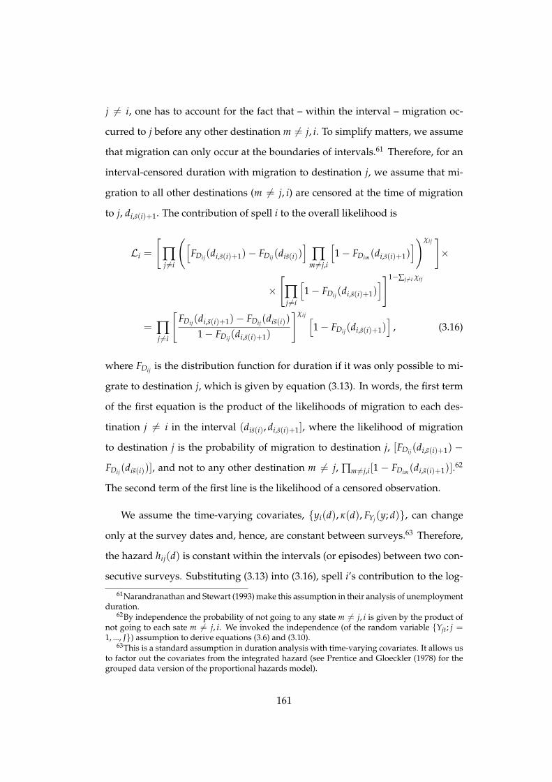
j 6= i, one has to account for the fact that – within the interval – migration oc-

curred to j before any other destination m 6= j, i. To simplify matters, we assume

that migration can only occur at the boundaries of intervals.61 Therefore, for an

interval-censored duration with migration to destination j, we assume that mi-

gration to all other destinations (m 6= j, i) are censored at the time of migration

to j, di,s(i)+1. The contribution of spell i to the overall likelihood is

Li =

[∏j 6=i

([FDij(di,s(i)+1)− FDij(dis(i))

]∏

m 6=j,i

[1− FDim(di,s(i)+1)

])χij]×

×[∏j 6=i

[1− FDij(di,s(i)+1)

]]1−∑j 6=i χij

= ∏j 6=i

[FDij(di,s(i)+1)− FDij(dis(i))

1− FDij(di,s(i)+1)

]χij [1− FDij(di,s(i)+1)

], (3.16)

where FDij is the distribution function for duration if it was only possible to mi-

grate to destination j, which is given by equation (3.13). In words, the first term

of the first equation is the product of the likelihoods of migration to each des-

tination j 6= i in the interval (dis(i), di,s(i)+1], where the likelihood of migration

to destination j is the probability of migration to destination j, [FDij(di,s(i)+1) −

FDij(dis(i))], and not to any other destination m 6= j, ∏m 6=j,i[1− FDim(di,s(i)+1)].62

The second term of the first line is the likelihood of a censored observation.

We assume the time-varying covariates, {yi(d), κ(d), FYj(y; d)}, can change

only at the survey dates and, hence, are constant between surveys.63 Therefore,

the hazard hij(d) is constant within the intervals (or episodes) between two con-

secutive surveys. Substituting (3.13) into (3.16), spell i’s contribution to the log-

61Narandranathan and Stewart (1993) make this assumption in their analysis of unemploymentduration.

62By independence the probability of not going to any state m 6= j, i is given by the product ofnot going to each sate m 6= j, i. We invoked the independence (of the random variable {Yjt; j =1, ..., J}) assumption to derive equations (3.6) and (3.10).

63This is a standard assumption in duration analysis with time-varying covariates. It allows usto factor out the covariates from the integrated hazard (see Prentice and Gloeckler (1978) for thegrouped data version of the proportional hazards model).

161

likelihood writes as

`i = ∑j 6=i

(χij log

[exp

(∫ di,s(i)+1

dis(i)

hij(ν)dν

)− 1

]−∫ di,s(i)+1

0hij(ν)dν

)(3.17)

= ∑j 6=i

(χij log

[exp

(hij(dis(i))[di,s(i)+1 − dis(i)]

)− 1]

−s(i)

∑s=0

hij(dis)[di,s+1 − dis]

)(3.18)

= ∑j 6=i

s(i)

∑s=0

(χij,s+1 log

[exp

(hij(dis(i))[di,s(i)+1 − dis(i)]

)− 1]

− hij(dis)[di,s+1 − dis]

), (3.19)

where χijs is an indicator variable that takes the value one if migration to state j

occurs before survey s and zero otherwise. The last term in equation (3.18) breaks

the integrated hazard with support [0, ds(i)+1] into a sum of integrated hazards

with support equal to the intervals (or episodes) between surveys [ds, ds+1]. We

then use our assumption that the hazard hij(d) is constant between surveys (or

within episodes) to take it outside the integral. This is known as episode splitting

and is necessary to account for the time-varying covariates.64 Equation (3.19)

follows because χijs = 0, ∀s ≤ s(i), and χij,s(i)+1 = 1 if χi = 1 and zero otherwise.

This final form of the log-likelihood is convenient since the joint likelihood for a

set of duration observations (where an observation is an episode within a spell)

is simply the sum of each observation’s contribution to the log-likelihood.65

64Episode splitting has a major benefit over simply using the last period an individual is ob-served in a spell. Indeed, although the final period of a spell is when the action happens (migrationif interval-censored), the individual is continuously making a choice whether to move of not dur-ing the spell and this is useful information. Although by definition no migration takes place withinthe spell, it is because we observe the time-varying explanatory variables (personal circumstancesand regional conditions) at each survey within the spell that these episodes serve as vital (withinindividual-spell) variation to help us explain why – for interval-censored spells – migration occursin the last period (or episode) and (for censored spells) it greatly increases the sample size.

65There is a problem with applying the log-likelihood in equation (3.19) to left-censored spellsbecause, by definition, we do not know the spell start date and, hence, we do not know durationat any survey preceding completion or right-censoring. We present results for the subsample thatdrops all left-censored spells.

162

Recall that we have multiple-spell data; that is, for some individuals we ob-

serve more than one spell (see Table 3.3).66 Let n index individuals and i(n)

denote the total number of spells for individual n. An individual may have an

unobserved propensity to migrate not captured by our model which will lead

to dependence in duration across spells of the same individual. In order to con-

trol for this we cluster standard errors at the individual-level. The log-likelihood

function for the sample is not the sum of the individual spell log-likelihood con-

tributions (due to the within-individual spell correlation and sampling weights)

but we assume that the solution to the pseudo-log likelihood

β = arg maxβ ∑n

i(n)

∑i

wi`i(β; data), (3.20)

is a reasonable estimate of the true parameter estimates β. In the above equation

wi is the PSID-supplied sampling weight for spell i and `i is given in equation

(3.19).67

We impose the restrictions implied by the structural model; that is, the haz-

ard hij(d) is given by equation (3.12), which is a function of the reservation in-

come given by the differential equation in (3.11). The differential equation for

the reservation income – net of moving costs – is solved recursively from time

T = 65 (retirement age in the U.S.) using numerical methods. Naturally we need

to generalise the model to make it applicable to empirical analysis. In particular,

we do not observe place attachment κ, the cost of moving cij, or counterfactual

income in spell i in the event that migration had not taken place. We now discuss

the parameterisation of κ and cij, and the prediction of post-migration counter-

factual income in spell i.

66An individual will have more than one duration spell if (in-sample) she migrates interstateor, due to missing values, we are forced to split a duration (where no change in state is reportedeither side of missing values) into two censored spells.

67Actually the PSID sampling weight varies across survey years s within spell i (individualsampling weights are updated in later survey waves to account for differential attrition) so itshould have a subscript s and be written inside the sum over s in `i.

163

The unknown κ’s are parameterised as follows. The initial value of κ, κ(1),

has a probability of taking on one of K values (or types). Since we do not know

which type the individual in spell i is, spell i’s contribution to the likelihood

becomes a mixture distribution over the K types

Li =K

∑k=1

πkLi(κk), (3.21)

where πk is the probability of type κk and ∑Kk=1 πk = 1.68 Both the parameter

vector of mass points {κk}Kk=1 and their corresponding probabilities {πk}K

k=1 are

to be estimated.69 For simplicity we assume K = 2 (low and high initial κ). In

addition, we assume that κ evolves with duration according to κ(d) = κkdβκ−1,

where βκ is common to all and is to be estimated.70 If βκ is greater (less) than one

then place attachment is monotonically increasing (decreasing) in duration.

The cost of moving from region i to j, cij ≥ 0, is assumed to be a linear func-

tion of distance, cij = c + βclij, where lij is the distance in kilometres between i

and j and (c, βc) are parameters to be estimated.

We predict counterfactual individual income in spell i at time t for the post-

migration period until retirement (age T = 65) based on (in-sample) estimates

of the labour income process. We estimate a model of individual labour income

using the full PSID sample of heads of households aged 16 to 64. We assume that

the log of labour income for individual n in spell i at time t follows

ln ynit = si + z′itθ + (si ∗ zit)′ϑ + g1(si ∗ tt) + τt + un + εit,

where si is the state of residence for spell i, zit is a vector of covariates, tt is a time

68This is analogous to studies of unemployment duration in the presence of worker hetero-geneity in non-market productivity (see, for example, Eckstein and Wolpin (1990)).

69This is identical to the Heckman and Singer (1984) non-parametric method of controlling forunobserved heterogeneity in duration analysis.

70Notice we assume duration starts from d=1, this is consistent with the definition of migrationas a change in location of primary residence for at least a year.

164

trend, τt is a year dummy, un is an individual fixed effect, and εit is an AR(1)

disturbance. The vector of covariates zit consists of a quadratic polynomial in

experience and a dummy for four or more years of college education. A prob-

lem with estimating this log-linear model is the presence of zeros in the labour

income series. The relevant literature on this typically advocates either recod-

ing the zeros to ones and use OLS, dropping the problem zero observations and

use OLS, or use the PPML estimator of Santos Silva and Tenreyro (2006, 2010).

We adopt the latter approach. The value of gjt in the present value factor Rjt in

equation (3.3) is estimated from the derivative of the log income process above

with respect to (linear) experience and the time trend. It is critical that the esti-

mates capture the growth in earnings with experience since, if not, then it will

confound our estimate of the duration-dependence of place attachment.

Clearly there are many covariates in addition to those that constitute the par-

simonious structural model of section 3.2 which one might expect to influence

the migration decision. Not only are we interested to know if and how these

additional covariates affect migration, failure to control for them will lead to

omitted variable bias. Further, since we will estimate κ(d) as unobserved (time-

varying) heterogeneity, it is paramount that we control for an exhaustive set of

observable explanatory variables. We control for a bunch of (time-varying) co-

variates including age, gender, race, marital status and whether the individual

has a college degree. Let these additional controls be stacked in the column vec-

tor xi(d).71 Since our search theory has nothing to say about these additional

covariates, we assume that the hazard function follows the proportional hazard

71Age, gender and race are ‘strictly exogenous’ with respect to migration; the ‘weak exogeneity’of education and marriage is due to them being predetermined – that is, measured at the start ofthe interval or episode and so prior to the migration decision. Note xi(d) does not include aconstant term because the constant term in the model is the initial value of κ, which is containedwithin hij(d).

165

(PH) model of Cox (1972) in respect to the control vector xi(d); that is,

hij(d, xi) = hij(d) exp[xi(d)′βx], (3.22)

where βx is a column vector of coefficients to be estimated. To be clear, xi(d)

contains neither a constant nor duration time dummies. We assume the con-

trol vector xi(d) can only change at survey dates and not between surveys for

the reason given above. To summarise, the maximum likelihood will estimate

the parameters {{κk}Kk=1, {πk}K

k=1, βκ, βc, βx}. We calibrate the sum of the rate

of time preference and the probability of death (r + φ) to 4 percent a year.72 The

maximum likelihood estimation does not identify these parameters (it would op-

timally set them to zero) since – in the model – death is indistinguishable from a

right-censored observation.

To provide a benchmark for the structural estimation we also present esti-

mates from a reduced-form model. The reduced-form model assumes a propor-

tional hazard

hr fij (d, zij) = ξdξ−1 exp[zij(d)′βz], (3.23)

where ξdξ−1 is the baseline hazard function, zij(d) is a vector of covariates for

spell i and destination j at duration d, and (ξ, βz) is a vector of parameters to

be estimated. The baseline hazard here implies a Weibull distribution for dura-

tion if the covariate vector zij(d) is time-invariant. If ξ is greater than one, then

the baseline hazard is increasing with duration; conversely if ξ is less than one,

then the baseline hazard is decreasing in duration. The covariate vector zij(d)

includes a constant term which can take on one of K = 2 values. The probability

72Estimates of the subjective rate of time preference vary widely across studies (see Fredericket al. (2002) for a survey) and typically are much higher than the market interest rate. Nonethe-less, 4 percent is consistent with the lower end of estimates of the rate of time preference fromthe macroeconomic literature (see, for example, Carroll and Samwick (1997) and Gourinchas andParker (2001)). It is also comparable to the post-tax return on capital in the U.S. of around 5 percent.

166

of these K = 2 values sum to one. This captures unobserved heterogeneity in a

manner analogous to that of κ(1) in the structural model and generates a mixed

distribution.73 The covariate vector zij(d) also includes the location parameter

of the destination-j income distribution, Ajt; current income, yit; the distance-to-

destination j, lij; age; and indicator variables for gender, race, marital status and

whether the individual has a college degree. Substituting equation (3.23) into

equation (3.17) and using the assumption that the covariate vector zij(d) is con-

stant within intervals, the contribution to the log-likelihood from spell i writes

as

`r fi = ∑

j 6=i

[χij log

(exp

[exp

(log[dξ

i,s(i)+1 − dξis(i)] + zij(dis(i))

′βz)]

− 1)−

s(i)

∑s=0

exp(

log[dξi,s+1 − dξ

is] + zij(dis)′βz

) ]

= ∑j 6=i

s(i)

∑s=0

[χij,s+1 log

(exp

[exp

(log[dξ

i,s(i)+1 − dξis(i)] + zij(dis(i))

′βz)]

− 1)− exp

(log[dξ

i,s+1 − dξis] + zij(dis)

′βz

) ]. (3.24)

Our Matlab code for the maximum likelihood estimation of the structural and

reduced-form models is given in Appendix 3.C.74,75 As a check to see whether

we have found a global or local maximum, we run the code for widely different

starting values and reassuringly all converged to the same solution.

73See Heckman and Singer (1984).74We used Matlab’s ‘fminsearch’ algorithm to find the minimum of (the neg-

ative of) the log-likelihood. The parameter estimates are accurate to 1E-6. Ourcode for the computation of clustered standard errors borrows heavily from MichaelRockinger’s code for White sandwiched standard errors within his ‘Max lik’ program (seehttp://www.hec.unil.ch/matlabcodes/econometrics.html), which we have extended to accountfor clustering.

75As a rough check that our Matlab code does what it is supposed to, we estimated the reduced-form model when there is just a single risk of migration (as opposed to the J destination competingrisks of migration) and compared this with the output of the same model using Stata’s ml com-mand. The parameter estimates and the clustered standard errors are identical. The output – notpresented here for brevity – is available on request.

167

3.3.4 Results

Table 3.5 presents the parameter estimates for the reduced-form model in equa-

tion (3.24). Clustered standard errors are displayed in parentheses. Consider the

estimates from the first column – it uses the full sample. The estimate of ξ is

close to zero and statistically significant, implying that the baseline hazard ex-

hibits strong negative duration-dependence. In other words, the migration rate

decreases as the length of time spent in a state increases, all else equal. This is

consistent with the Kaplan-Meier empirical hazard rate we presented in Figure

3.3. Recall that all the other covariates enter the hazard function in proportion to

the baseline hazard. Therefore, to isolate the effect of a change in a covariate we

look at the ratio of two hazards with different values for the covariate of interest,

while keeping the values of all other covariates the same. For example, if we

want to look at the effect of a change in z1 on the hazard in equation (3.23) then

we compute the hazard ratiohr f

ij (d,z|z1=a+µ)

hr fij (d,z|z1=a)

= exp(βz1 µ), where µ is a constant

measured in the units of z1. If, however, z1 is log-transformed, then we look at

the hazard ratiohr f

ij (d,z| log(z1)=log(µa))

hr fij (d,z| log(z1)=log(a))

= exp(βz1 log(µ)) where µ is a multiple of

z1. The two destination-specific variables (distance-to-destination, lij, and the lo-

cation parameter of the estimated Frechet income distribution in the destination,

Ajt) and income yit are log-transformed in order to help with convergence of the

solver.76 Generally speaking, the remaining parameter estimates are consistent

with the empirical literature on the determinants of migration. The probability

of migration to a destination falls as the distance to that destination increases.

The coefficient estimate on distance of -0.65 implies that – when comparing two

destination states where the first is 10 percent nearer than the second – the indi-

vidual is 7 percent more likely to migrate to the first than the second destination,

all else equal.77 Therefore, the distance between the current state and a potential

76It is well-known that convergence is aided if the variables are of similar scale.77The ratio of the two hazards is exp(−0.65 log(0.9)) = 1.07.

168

destination is a substantial deterrent to migration. The coefficient estimate on

log Ajt is positive and significant. That is, the effect of an increase in the location

parameter of a destination’s income distribution is to increase the probability of

migration to that destination. The remaining covariates pertain to personal cir-

cumstances. The estimate on current labour income is not statistically different

from zero. The migration rate is decreasing in age: an increase in age of 10 years

reduces the migration rate by 7 percent, ceteris paribus. A female is 47 percent

less likely to migrate than a male. A black individual is 48 percent less likely to

migrate than a non-black. Marriage and a college degree are – surprisingly – not

statistically significant. Finally, there is no evidence for unobserved heterogene-

ity in the constant term since, the estimates of the two constant terms are almost

identical.78

Columns 2 and 3 of Table 3.5 divide the sample into those spells that took

place in the state the individual grew-up and those spells that took place in some

other (host) state, respectively.79 One might expect the reasons for migration and

their relative importance to differ depending on whether the individual resides

in the state he or she grew-up or a host state. In particular, theoretically it is un-

clear whether the migration rate in a host state would increase or decrease with

duration. A positive dependence would arise if, for example, the longer an indi-

vidual stays in the host state the higher is the cost of being away from the state

he or she grew-up.80 Here one would argue that the psychic cost of being away

78Note the estimation forces the probability of a type 1 individual to lie between zero andone by setting the probability of a type 1 individual equal to exp(b)/(1 + exp(b)), where b is theestimate given in Table 3.5 with the label ‘prob type 1’. Therefore the estimate of -2.97E-2 equatesto a probability of a type 1 individual of 49 percent. One could use the delta method to providethe corresponding standard error but we know the estimate is not statistically different from 50percent.

79For 219 spells (629 observations) we do not know the state the individual grew up in and,hence, the number of observations for the grew-up and host subsamples do not sum to the numberof observations in the full sample.

80In an early theoretical contribution, Hill (1987) assumes the probability of returning home isincreasing in the period of time spent away.

169

TABLE 3.5

MAXIMUM LIKELIHOOD ESTIMATES OF THE REDUCED-FORMMODEL

All states Grew-up states Host states

ξ 1.09E-5 2.87E-7 7.50E-2(5.78E-9) (3.11E-9) (4.95E-2)

log(lij) -0.650 -0.760 -0.676(3.93E-2) (7.88E-2) (4.02E-2)

log(Ajt) 0.186 3.30E-2 0.198(3.49E-2) (6.80E-2) (5.64E-2)

log(yit + 1) 4.57E-4 3.29E-3 -2.74E-2(1.20E-2) (2.17E-2) (1.27E-2)

age -7.18E-3 -6.50E-3 -2.32E-2(2.88E-3) (5.65E-3) (3.65E-3)

female -0.641 -0.261E-1 -0.747(0.116) (0.247) (0.120)

black -0.663 -0.244 -0.560(0.136) (0.174) (0.135)

married -9.37E-2 0.229 -6.57E-2(9.36E-2) (0.236) (8.68E-2)

degree 4.81E-2 0.663 0.320(0.122) (0.196) (7.78E-2)

type 1 cons 7.762 11.942 0.479(9.65E-2) (0.463) (0.185)

type 2 cons 7.756 11.939 0.479(9.63E-2) (0.464) (0.184)

prob type 1 -2.97E-2 -1.03E-2 -2.88E-2(0.160) (0.433) (0.236)

observations 149,084 100,750 47,705log-likelihood -369,840.8 -74,694.5 -274,560.2

Note: Standard errors (in parentheses) are robust and clustered at theindividual level to allow for correlation across duration spells for thesame individual.

170

from family and friends is increasing in the time spent away from them. On the

other hand, a negative duration dependence can arise if, for example, a famil-

iarity with surroundings and the establishment of social networks grows with

time spent in the host state. It is ultimately an empirical question. We find that

– although our estimate of ξ is higher in the host than the grew-up subsample –

it remains comfortably less than one, implying the migration rate exhibits nega-

tive duration-dependence in both the grew-up and host subsamples. Therefore,

the reduced-form estimates suggest that assimilation dominates and that place

attachment increases with duration. There are other notable differences between

the grew-up and host subsamples. Distance appears to have slightly less of a

negative effect on migration for someone residing in a host state. This would

make sense if migrants build-up an ability to absorb the extra costs associated

with migrating longer distances as a result of earlier migrations. The location

parameter of the destination income distribution is statistically insignificant for

the grew-up subsample and positive for the host subsample.81 This may imply

that former migrants are much more sensitive to the opportunities in potential

destinations and they target states with higher income. The coefficient estimate

of labour income in the host subsample is significant and negative whereas it is

insignificant in the grew-up sample. This might suggest that former migrants

are sensitive to current income and a bad income shock increases the migration

rate. Age is a bigger deterrent to migration in the host subsample. There is a

big difference in the effect of gender on migration across the two subsamples.

In the grew-up subsample gender has no significant effect whereas in the host

subsample females are much less likely to migrate. One has to be careful when

interpreting this result because we restricted our sample to heads of households

and in the PSID the household head is – by convention – the male head unless

81Recall that 81 percent of the interval-censored spells (which are crucial for identification) takeplace in a host state; hence, it is unsurprising that the estimates from the grew-up subsample lacksignificance.

171

no obvious male head is present. Finally, a college degree is significant and pos-

itively effects the migration rate for both the grew-up and host subsamples.

As mentioned, for left-censored spells we do not know true duration at any

point during the spell and therefore our estimates in Table 3.5 are based on in-

sample duration for left-censored spells (and, hence, underestimate true dura-

tion), which account for a substantial 86 percent of all observations. Of particular

concern is our estimate of ξ which is directly a function of duration. Therefore,

Table 3.6 presents the output for the reduced-form model using the subsample

that drops all left-censored spells. As expected, the estimates for ξ are higher,

although they remain substantially less than one.82 Therefore, our earlier find-

ing holds, the estimate of the baseline hazard suggest that place attachment is

increasing with duration in a U.S. state. Of course, this assumes that the baseline

hazard captures place attachment and not some other (time-dependent) unob-

servable.

Table 3.7 presents the output of the structural estimation for the subsample

that drops left-censored spells. Again we present estimates for the combined

sample of grew-up and host states (in column 1) and the disaggregated esti-

mates for the grew-up and host subsamples (in columns 2 and 3 respectively).

The Matlab code scales some of the parameters to help with convergence of

the solver. More specifically, the estimate of κ1 in Table 3.7 needs to be multi-

plied by 10,000; and the estimate of the probability of κ1 (denoted π) is equal to

exp(b)/(1 + exp(b)) where b is the estimate reported in Table 3.7 under π. We

82The intuition for why the removal of left-censored spells increases ξ is as follows. Left (andright) censored spells impact the hazard through their effect on the numbers at risk of migrationat each level of duration. They, of course, do not contribute to the numbers that actually migrateat any level of duration. Therefore, left (and right) censored spells simply scale the hazard. Giventhat in-sample duration of left-censored spells underestimates true duration and that the numberat risk of migration is necessarily lower for higher durations, they tend to scale the lower tail ofduration too lightly (they are scaling low durations with a low number that should be used toscale higher durations) and consequently this results in a lower estimate of ξ (or higher convexityof the baseline hazard).

172

TABLE 3.6

MAXIMUM LIKELIHOOD ESTIMATES OF THE REDUCED-FORMMODEL FOR SUBSAMPLE THAT DROPS LEFT-CENSORED

SPELLS

All states Grew-up states Host states

ξ 0.126 0.143 0.224(4.10E-2) (9.44E-2) (4.90E-2)

log(distij) -0.683 -0.827 -0.668(3.75E-2) (9.51E-2) (3.97E-2)

log(Ajt) 0.145 -0.416 0.354(3.81E-2) 0.694 (5.09E-2)

log(yit + 1) -0.009 0.034 -0.035(0.011) (0.027) (0.012)

age -1.75E-2 -1.40E-2 -2.67E-2(3.07E-3) (7.63E-3) (3.75E-3)

female -0.264 -0.208 -0.284(0.088) (0.203) (0.097)

black -0.256 -0.146 -0.235(0.096) (0.207) (0.112)

married -0.194 -0.254 -0.205(6.80E-2) (0.166) (7.41E-2)

degree 0.059 0.155 -0.034(5.99E-2) (0.155) (6.65E-2)

type 1 cons 0.894 6.412 -1.270(0.246) (7.571) (0.542)

type 2 cons 0.894 6.412 -1.270(0.246) (7.569) (0.542)

prob type 1 0.002 0.121 -0.021(0.219) (0.491) (0.188)

observations 20593 7840 12666log-likelihood -304532.8 -58056.3 -242893.2

Note: The sample excludes all left-censored spells. Standard errors (inparentheses) are robust and clustered at the individual level.

173

first turn to the parameter estimates of initial place attachment: κ1 and κ2. The

estimate of κ1 in the first column implies that the value of place attachment for

a type 1 individual has an income-equivalent of 142,800 dollars in 1999 prices.

The estimate of κ1 in the grew-up subsample is even higher at 223,320 dollars

and, in the host subsample it is lower but still a massive 106,170 dollars. Such

a value of place attachment means migration is prohibitively costly. In contrast,

the estimates of κ2 are close to zero in all three samples. The estimates of κ2

are just 4.5, 10.3 and 2.3 dollars in the combined, grew-up and host samples, re-

spectively. Therefore, the estimates imply that initial place attachment is either

extremely high or approximately zero. The estimates of π are not statistically

different from 0.5 in all three samples. Therefore, around half of the popula-

tion has an initial place attachment that prohibits migration, and the other half

have no initial attachment at all. We next turn to the estimate of the duration-

dependence of place attachment. We find that βκ is positive and greater than one

in the combined sample (column 1). This implies place attachment is increasing

with duration, which is consistent with the reduced-form estimates. However,

the estimates for the grew-up and host subsamples are wildly different. In both

the grew-up and host subsamples, place attachment is decreasing in duration.

Moreover, place attachment falls away much more strongly in the host subsam-

ple than in the grew-up subsample. It suggests that migrants get itchy feet to

move again, possibly to return to a state that they previously resided in. The

remaining estimates suggest that the cost of moving is increasing in distance-to-

destination. Also, the probability of migration is decreasing in age and higher

for someone with a college degree. Finally, the coefficient estimates on the indi-

cator variables for gender, marriage and race have the opposite sign to both the

reduced-form estimates and prior expectations.

In summary, the reduced-form estimates strongly suggest that place attach-

174

TABLE 3.7

STRUCTURAL MAXIMUM LIKELIHOOD ESTIMATES FORSUBSAMPLE THAT DROPS LEFT-CENSORED SPELLS

All states Grew-up states Host states

κ1 14.280 22.332 10.617(6.17E-5) (5.17E-6) (5.47E-6)

κ2 4.554 10.300 2.288(8.29E-4) (3.44E-5) (2.26E-3)

π 4.44E-4 -9.79E-4 -5.80E-4(0.783) (0.405) (0.257)

βκ 2.439 0.930 -3.358(6.61E-5) (1.40E-5) (8.23E-6)

log(lij) 4.40E-4 2.50E-4 1.22E-3(2.54E-4) (4.72E-5) (9.59E-5)

c 1.03E-3 5.39E-3 1.12E-2(2.07E-4) (2.62E-5) (2.07E-5)

age -1.48E-2 -1.70E-2 -1.69E-2(3.30E-3) (5.56E-3) (3.85E-3)

female 1.083 0.611 1.347(0.177) (0.306) (0.218)

black 0.376 0.340 0.383(0.142) (0.255) (0.179)

married 0.970 0.308 1.242(0.165) (0.271) (0.201)

degree 0.564 0.542 0.537(9.34E-2) (0.196) (0.108)

observations 20,593 7,840 12,666log-likelihood -499,920.3 -92,969.7 -403,737.2

Note: The sample excludes all left-censored spells. Standard errors (inparentheses) are robust and clustered at the individual level.

175

ment is increasing with the length of stay in a region. This is true for the sub-

sample of individuals that reside in a host state as well as the subsample that

live in the state they grew-up in. In stark contrast, the structural estimates of

place attachment suggest the opposite; that is, place attachment falls with du-

ration both in a host state and the state that an individual grew-up in. Further,

around half the population have an initial value for place attachment that im-

plies migration is prohibitively costly. It is unclear how much weight one should

attach to our structural estimates given that they differ so wildly from those of

the reduced-form model. Nonetheless, it suggests more work is needed on what

is an important and under-researched topic.

3.4 Conclusion

This chapter is motivated by a desire to quantify unobserved place attachment;

that is, the emotional bonds and feelings one has with the region of residence.

While a number of studies on the determinants of migration have found that

distance-to-destination has a strong negative effect on migration, little is known

about the costs associated with leaving the current region of residence that are

independent of distance. More specifically, in order to determine the numbers

of people that are at risk of migration, one would like to know how place at-

tachment is distributed, both across individuals and time spent in a particular

area.

We present a model of migration where spatial job search determines the

propensity to migrate to a particular destination. An important contribution

is that we extend the standard job search model to a situation where multiple

labour markets are searched. Using extreme value theory we derive a structural

equation for the destination-specific migration (or hazard) rate. This is expressed

176

as a function of current and future income, place attachment and the distribution

of income offers in each destination.

We then estimate the structural model for a sample of individual durations in

a U.S. state. The duration data is from the Panel Study of Income Dynamics. The

findings are surprising. While the reduced-form estimates suggest that place at-

tachment is increasing in the length of stay in a U.S. state, the structural estimates

suggest the opposite. More research is needed to verify this relationship.

References

AGUIRREGABIRIA, V. AND P. MIRA (2010): “Dynamic discrete choice structuralmodels: A survey,” Journal of Econometrics, 156, 38–67.

BASKER, E. (2003): “Education, Job Search and Migration,” Working paper, Uni-versity of Missouri - Columbia.

BECKER, G. S. (1964): Human Capital: A Theoretical and Empirical Analysis withSpecial Reference to Education, New York: National Bureau of Economic Re-search.

BECKETTI, S., W. GOULD, L. LILLARD, AND F. WELCH (1988): “The Panel Studyof Income Dynamics after Fourteen Years: An Evaluation,” Journal of LaborEconomics, 6, 472–492.

BORJAS, G. J. (1987): “Self-Selection and the Earnings of Immigrants,” AmericanEconomic Review, 77, 531–553.

CARROLL, C. AND A. SAMWICK (1997): “The Nature of Precautionary Wealth,”Journal of Monetary Economics, 40, 41–71.

COULSON, N. E., D. LAING, AND P. WANG (2001): “Spatial Mismatch in SearchEquilibrium,” Journal of Labor Economics, 19, 949–972.

COX, D. R. (1972): “Regression Models and Life-Tables,” Journal of the Royal Sta-tistical Society. Series B, 34, 187–220.

DJAJIC, S. AND R. MILBOURNE (1988): “A General Equilibrium Model of Guest-Worker Migration: The Source Country Perspective,” Journal of InternationalEconomics, 25, 335–351.

DUSTMANN, C. (2003): “Return Migration, Wage Differentials, and the OptimalMigration Duration,” European Economic Review, 47, 353–369.

177

DUSTMANN, C. AND Y. WEISS (2007): “Return Migration: Theory and EmpiricalEvidence from the UK,” British Journal of Industrial Relations, 45, 236–256.

EATON, J. AND S. KORTUM (2002): “Technology, Geography, and Trade,” Econo-metrica, 70, 1741–1779.

ECKSTEIN, Z. AND K. WOLPIN (1989): “The specification and estimation of dy-namic stochastic discrete choice models,” Journal of Human Resources, 24, 562–598.

ECKSTEIN, Z. AND K. I. WOLPIN (1990): “Estimating a Market EquilibriumSearch Model from Panel Data on Individuals,” Econometrica, 58, 783–808.

ELBERS, C. AND G. RIDDER (1982): “True and Spurious Duration Dependence:The Identifiability of the Proportional Hazard Model,” Review of Economic Stud-ies, 49, 403–409.

FAHR, R. AND U. SUNDE (2002): “Employment Status, Endogenous RegionalMobility, and Spatial Dependencies in Labor Markets,” Discussion Paper 521,IZA.

FLINN, C. AND J. HECKMAN (1982): “New Methods for Analyzing StructuralModels of Labor Force Dynamics,” Journal of Econometrics, 18, 115–168.

FREDERICK, S., G. LOEWENSTEIN, AND T. O’DONOGHUE (2002): “Time Dis-counting and Time Preference: A Critical Review,” Journal of Economic Litera-ture, 40, 351–401.

GALLAWAY, L. E. (1969): “Age and Labor Mobility Patterns,” Southern EconomicJournal, 36, 171–180.

GINSBERG, R. B. (1973): “Stochastic models of residential and geographic mobil-ity for heterogeneous populations,” Environment and Planning, 5, 113–124.

GOURINCHAS, P.-O. AND J. PARKER (2001): “The Empirical Importance of Pre-cautionary Saving,” American Economic Review, 91, 406–412.

GOUSKOVA, E., S. G. HEERINGA, K. MCGONAGLE, AND R. F. SCHOENI (2008):“Revised Longitudinal Weights 1993-2005,” Technical report, Panel Study ofIncome Dynamics.

GREENWOOD, M. J. (1975): “Research on Internal Migration in the United States:A Survey,” Journal of Economic Literature, 13, 397–433.

HARRIS, J. R. AND M. P. TODARO (1970): “Migration, Unemployment and De-velopment: A Two-Sector Analysis,” American Economic Review, 60, 126–142.

HECKMAN, J. AND B. SINGER (1984): “A Method for Minimizing the Impact ofDistributional Assumptions in Econometric Models for Duration Data,” Econo-metrica, 52, 271–320.

178

HERZOG JR, H. W., A. M. SCHLOTTMANN, AND T. P. BOEHM (1993): “Migrationas Spatial Jobsearch: A Survey of Empirical Findings,” Regional Studies, 27,327–340.

HILL, J. K. (1987): “Immigrant Decisions Concerning Duration of Stay and Mi-gratory Frequency,” Journal of Development Economics, 25, 221–234.

JENKINS, S. P. (2005): “Survival Analysis,” Working paper, Institute for Socialand Economic Research, University of Essex, Colchester, UK.

KEANE, M. P. AND K. I. WOLPIN (2009): “Empirical applications of discretechoice dynamic programming models,” Review of Economic Dynamics, 12, 1–22.

KENNAN, J. AND J. R. WALKER (2003): “The Effect of Expected Income on Indi-vidual Migration Decisions,” Working Paper 9585, NBER.

KING, M., S. RUGGLES, J. T. ALEXANDER, S. FLOOD, K. GENADEK, M. B.SCHROEDER, B. TRAMPE, AND R. VICK (2010): “Integrated Public Use Mi-crodata Series, Current Population Survey: Version 3.0,” Minneapolis, MN:Minnesota Population Center [producer and distributor], [Machine-readabledatabase].

KLEIBER, C. AND S. KOTZ, eds. (2003): Statistical Size Distributions in Economicsand Actuarial Sciences, New York: Wiley-Interscience.

LANCASTER, T. (1979): “Econometric Methods for the Duration of Unemploy-ment,” Econometrica, 47, 939–956.

LIPPMAN, S. A. AND J. J. MCCALL (1976): “The Economics of Job Search: ASurvey,” Economic Inquiry, 14, 155–189.

MCCALL, B. P. AND J. J. MCCALL (1987): “A Sequential Study of Migration andJob Search,” Journal of Labor Economics, 5, 452–476.

MESNARD, A. (2004): “Temporary migration and capital market imperfections,”Oxford Economic Papers, 56, 242–262.

MIRON, J. R. (1978): “Job-search perspectives on migration behaviour,” Environ-ment and Planning A, 10, 519–535.

NARANDRANATHAN, W. AND M. B. STEWART (1993): “Modelling the probabil-ity of leaving unemployment: competing risk models with flexible base-linehazards,” Applied Statistics, 42, 63–83.

ORTEGA, J. (2000): “Pareto-Improving Immigration in an Economy with Equi-librium Unemployment,” Economic Journal, 110, 92–112.

PICKLES, A. AND P. ROGERSON (1984): “Wage Distributions and Spatial Prefer-ences in Competitive Job Search and Migration,” Regional Studies, 18, 131–142.

179

PRENTICE, R. L. AND L. A. GLOECKLER (1978): “Regression Analysis ofGrouped Survival Data with Application to Breast Cancer Data,” Biometrics,34, 57–67.

RAFFELHSCHEN, B. (1992): “Labor migration in Europe: Experiences from Ger-many after unification,” European Economic Review, 36, 1453–1471.

RELPH, E., ed. (1976): Place and Placelessness, London: Pion.

ROGERSON, P. AND R. D. MACKINNON (1981): “A Geographical Model of JobSearch, Migration and Unemployment,” Papers in Regional Science, 48, 89–102.

ROGERSON, R., R. SHIMER, AND R. WRIGHT (2005): “Search-Theoretic Modelsof the Labor Market: A Survey,” Journal of Economic Literature, XLIII, 959–988.

RUST, J. (1994): “Structural Estimation of Markov Decision Processes,” in Hand-book of Econometrics, ed. by R. Engle and D. McFadden, Amsterdam: NorthHolland, 3081–3143.

SANTOS SILVA, J. AND S. TENREYRO (2006): “The log of gravity,” The Review ofEconomics and Statistics, 88, 641–658.

——— (2010): “On the existence of the maximum likelihood estimates in Poissonregression,” Economics Letters, 107, 310–312.

SCHWARTZ, A. (1973): “Interpreting the Effect of Distance on Migration,” Journalof Political Economy, 81, 1153–1169.

——— (1976): “Migration, Age, and Education,” Journal of Political Economy, 84,701–720.

SJAASTAD, L. A. (1962): “The Costs and Returns of Human Migration,” Journalof Political Economy, 70, 80–93.

TODARO, M. P. (1969): “A Model of Labor Migration and Urban Unemploymentin Less Developed Countries,” American Economic Review, 59, 138–148.

TOPEL, R. H. (1986): “Local Labor Markets,” Journal of Political Economy, 94,S111–S143.

VAN DEN BERG, G. J. (1990): “Nonstationarity in Job Search Theory,” Review ofEconomic Studies, 57, 255–277.

YANG, D. (2006): “Why Do Migrants Return To Poor Countries? Evidence FromPhilippine Migrants Responses To Exchange Rate Shocks,” Working Paper12396, NBER.

ZABEL, J. E. (1998): “An Analysis of Attrition in the PSID and SIPP with anApplication to a Model of Labor Market Behavior,” Journal of Human Resources,33, 479–506.

180

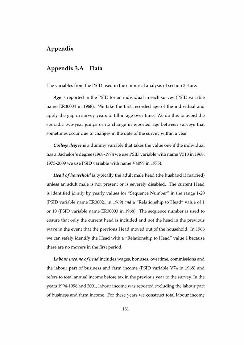
Appendix

Appendix 3.A Data

The variables from the PSID used in the empirical analysis of section 3.3 are:

Age is reported in the PSID for an individual in each survey (PSID variable

name ER30004 in 1968). We take the first recorded age of the individual and

apply the gap in survey years to fill in age over time. We do this to avoid the

sporadic two-year jumps or no change in reported age between surveys that

sometimes occur due to changes in the date of the survey within a year.

College degree is a dummy variable that takes the value one if the individual

has a Bachelor’s degree (1968-1974 we use PSID variable with name V313 in 1968;

1975-2009 we use PSID variable with name V4099 in 1975).

Head of household is typically the adult male head (the husband if married)

unless an adult male is not present or is severely disabled. The current Head

is identified jointly by yearly values for “Sequence Number” in the range 1-20

(PSID variable name ER30021 in 1969) and a “Relationship to Head” value of 1

or 10 (PSID variable name ER30003 in 1968). The sequence number is used to

ensure that only the current head is included and not the head in the previous

wave in the event that the previous Head moved out of the household. In 1968

we can safely identify the Head with a “Relationship to Head” value 1 because

there are no movers in the first period.

Labour income of head includes wages, bonuses, overtime, commissions and

the labour part of business and farm income (PSID variable V74 in 1968) and

refers to total annual income before tax in the previous year to the survey. In the

years 1994-1996 and 2001, labour income was reported excluding the labour part

of business and farm income. For these years we construct total labour income

181

by summing labour income excluding business and farm income (variable name

ER4140 in 1994), farm income (ER4117 in 1994) and the labor portion of business

income (ER4119 in 1994). Labour income is expressed in constant 1999 dollars

using the CPI-U. Survey respondents are asked about their labour income in the

previous year. We forward labour income by one survey wave to account for this

although it is, of course, imperfect for the biennial surveys post-1997.

Sampling weights are inverse (ex-ante) sampling probability weights sup-

plied by the PSID. From 1968 to 1989 we use the “Core Individual Weight”

(variable name ER30019 in 1968); 1990-1992 the “Combined Core-Latino Weight”

(ER30688 in 1990); 1993-1995 the “Combined Core-Latino Sample Longitudinal

Weight” (ER30866 in 1993); 1996 we use the “Core Sample Individual Longitu-

dinal Weight” (ER33318) and post-1996 we use the “Combined Core-Immigrant

Sample Individual Longitudinal Weight” (ER33430 in 1997).

Year of death is available in the PSID Death File (variable name ER32050).

State is recorded in the PSID family files. Prior to 1985, states were coded

according to the GSA classification (variable name V93 in 1968) and from 1985

classified using the FIPS system (variable name V12380 in 1985). We coverted the

FIPS codes to the GSA classification.

State grew up is the state the respondent spent ‘most of the years age 6 to

16’. Prior to 1994 the state was coded using the GSA classification (variable name

V311 in 1968) and since 1997 used the FIPS code (variable name ER11842 in 1997).

182

Appendix 3.B Fitting a Frechet distribution to the Empiri-

cal Income Distribution

We fit the Frechet distribution separately for each state-year to minimise the

Kolmogorov-Smirnov statistic between the theoretical Frechet and the empirical

income distribution. The empirical income distribution is estimated using our

sample of individual incomes from the March Current Population Survey (CPS).

In the first run of the minimisations we allow both the location parameter for

state j in year t, Ajt, and the scale parameter, αjt, to depend on the state and year.

However, the theoretical model of section 3.2 assumes that the scale parameter

αjt is the same for all j, t. Therefore, to determine the constant scale parameter

for all states and all years, we simply took the average. The result is α = 1.1136.

This constraint does not appear to be too restrictive because the estimates of αjt

are not very different across states and years. We then re-run the estimations for

the location parameter Ajt for when α is constant. In doing this, we allow Ajt

to depend on experience, experience squared and whether the individual has a

college degree or not.83 The parameter estimates are then used to predict the

destination-specific income distribution that the PSID individual draws from in

each year. These parameter estimates enter directly into the differential equation

for the reservation income in spell i at time t. When an individual does not reach

age 64 (the terminal condition) until after 2010 (the latest year the CPS is avail-

able), we extrapolate linearly using the estimates of Ajt between 2002 and 2010

to predict values for t > 2010.

In estimating the empirical income distribution using the CPS data, we im-

pose some sample selection rules. First, since the domain of the two-parameter

Frechet distribution is the set of positive real numbers, we need to deal with the

83Prior to 1992 the CPS reports years of education and not categorical education such aswhether the individual has a Bachelor’s degree. We assume those individuals with four or moreyears of college have obtained a college degree.

183

existence of non-positive income observations.84 We simply drop the 438,734

observations with non-positive income. Second, we restrict the sample to those

individuals aged between 16 and 64 and drop the 421 observations with negative

CPS sampling weights. This leaves us with 3,841,014 observations for the 51x42

state-year pairs. The IPUMS-CPS does not report whether the CPS income data

has been top-coded and leaves this to the user to determine. We inspected the

upper tail of the empirical income distribution in each year for evidence of top-

coding. We could not find any evidence of top-coding for the wages and salaries

series, which is used for the estimations.85 In addition, between 1968 and 1975

not all U.S. states were identified separately, the CPS only recorded the largest 11

states and the others were grouped by proximity into groups of between 2 and 8

states. We estimated the income distribution for these groups and then assigned

the same parameter values to all constituent states. Finally, income is lagged to

account for the fact that the CPS income data refers to the previous year and,

income is deflated using the CPI-U and expressed in 1999 dollars.

A number of questions suggest themselves. First, is the Frechet distribution a

good fit to the empirical state-year income distribution? Is it a better fit than the

Lognormal? Is maximum likelihood or minimising the Kolmogorov-Smirnov

statistic the best tool for fitting the theoretical Frechet to the empirical income

distribution? To assess this, Figure 3.5 plots the cumulative distribution func-

tion for wages and salaries in 1990 for California (3.5a) and New York (3.5b),

along with the fitted Frechet and Lognormal distribution. For both the Frechet

and Lognormal, the graphs display the fitted distribution from maximum likeli-

hood estimation (MLE) and minimising the Kolmogorov-Smirnov (KS) statistic.

Figure 3.6 does the same for total personal income. In summary we note that

84The generalised 3-parameter Frechet distribution with the third parameter controlling theminimum can handle non-positive income observations but – to be consistent with the theoreticalmodel – we do not follow this path.

85Evidence of top-coding would be a sharp rise in the number of cases at the highest incomerecorded. We do not find this.

184

minimising the KS statistics visually gives a better fit to the empirical income

distribution than maximum likelihood estimation. Further, there is not much

between the goodness of fit for the Frechet and Lognormal distributions.

FIGURE 3.5

FITTING A THEORETICAL DISTRIBUTION TO THE EMPIRICAL DISTRIBUTION OF WAGESAND SALARIES IN CALIFORNIA AND NEW YORK, 1990

a) CALIFORNIA, 1990 b) NEW YORK, 1990

FIGURE 3.6

FITTING A THEORETICAL DISTRIBUTION TO THE EMPIRICAL DISTRIBUTION OFPERSONAL INCOME IN CALIFORNIA AND NEW YORK, 1990

a) CALIFORNIA, 1990 b) NEW YORK, 1990

185

Appendix 3.C Matlab Code for the Structural Estimation

% This is the main program. It returns Maximum Likelihood estimates ...

for the parameters of the structural model.

clear all;

sample = 'sample2'; % sample2 is the dataset that drops all ...

left−censored spells

% maximise likelihood

[b1 se1 N1 logL1 exit1] = ml(sample, 'All');

[b2 se2 N2 logL2 exit2] = ml(sample, 'Grewup');

[b3 se3 N3 logL3 exit3] = ml(sample, 'Host');

out = horzcat(b1,se1, b2,se2, b3,se3);

disp(num2str(out)); % display results

% ml.m is the program that generates Maximum Likelihood estimates ...

and their corresponding standard errors. Standard errors are ...

clustered at the individual level. ml.m is called by the main ...

program.

function [bhat se N logL exit] = ml(sample, state)

% load data

if strcmp(sample,'sample2');

load sample2.dat

load sample2 ext.dat

sample = sample2;

sample ext = sample2 ext;

clearvars sample2 sample2 ext

else

load sample1.dat

load sample1 ext.dat

sample = sample1;

sample ext = sample1 ext;

clearvars sample1 sample1 ext

186

end

% define subsample

if strcmp(state,'Host');

disp('Host states');

row = find(sample(:,216)==0 | sample(:,216)==99);

sample(row,:) = [] ; % host subsample

row = find(sample ext(:,158)==0 | sample ext(:,158)==99);

sample ext(row,:) = [] ; % host subsample

elseif strcmp(state,'Grewup')

disp('Grew up states');

row = find(sample(:,216)==1 | sample(:,216)==99);

sample(row,:) = [] ; % grew−up subsample

row = find(sample ext(:,158)==1 | sample ext(:,158)==99);

sample ext(row,:) = [] ; % grew−up subsample

else

disp('All states'); % default is all states

end

% define variables

n = sample(:,1); % individual id, used for clustering ...

standard errors

id = sample(:,2); % spell id

w = sample(:,3); % sampling weight

dl = sample(:,4); % duration, lower limit of interval

du = sample(:,5); % duration, upper limit of interval

age = sample(:,7); % age

X = sample(:,7:11); % additional covariates: age, female, ...

black, married, degree

dist = sample(:,12:62); % distance between states

A = sample(:,63:113); % location parameter estimate of Frechet ...

income distribution in the 51 US states

g = sample(:,114:164); % expected growth rate of income in the 51 ...

US states

chi = sample(:,165:215); % censoring indicator for the 51 US states

clearvars sample

187

% drop option of moving to current state

dist1 = zeros(size(dist,1),size(dist,2)−1);

A1 = zeros(size(dist1));

g1 = zeros(size(dist1));

chi1 = zeros(size(dist1));

index = (dist>0); % logical indexing − by definition current state ...

has dist=0

for i=1:size(dist,1)

distrow = dist(i,:);

Arow = A(i,:);

grow = g(i,:);

chirow = chi(i,:);

dist1(i,:) = distrow(index(i,:)); % keeps the cells with dist>0

A1(i,:) = Arow(index(i,:));

g1(i,:) = grow(index(i,:));

chi1(i,:) = chirow(index(i,:));

end

dist=dist1; A=A1; g=g1; chi=chi1;

clearvars dist1 A1 g1 chi1

% define the variables used to solve the differential equation for ...

the reservation income

s = sample ext(:,1); % spell id (= id above but extended ...

to age 64 for each spell)

dt = sample ext(:,2); % duration time (= dl above but ...

extended to age 64 for each spell)

y = sample ext(:,3); % labour income (observed during ...

spell and predicted to age 64)

agee = sample ext(:,4); % age

a = sample ext(:,5:55); % location parameter estimate of ...

Frechet income distribution (extrapolated to age 64)

dist2 = sample ext(:,56:106); % distance between states extended ...

to age 64

ge = sample ext(:,107:157); % expected growth rate of income

clearvars sample ext

188

% drop option of moving to current state for differential equation data

dist3 = zeros(size(dist2,1),size(dist2,2)−1);

A3 = zeros(size(dist3));

g3 = zeros(size(dist3));

index = (dist2>0); % logical indexing − by definition current ...

state has dist=0

for i=1:size(dist2,1)

distrow = dist2(i,:);

Arow = a(i,:);

grow = ge(i,:);

dist3(i,:) = distrow(index(i,:)); % keeps the cells with dist>0

A3(i,:) = Arow(index(i,:));

g3(i,:) = grow(index(i,:));

end

dist2=dist3; a=A3; ge=g3;

clearvars dist3 A3 g3

% set array dimensions

[N,J] = size(A); % N= # observations, J= # US states

M = size(y,1); % # observations to age 64

% set parameter values

T = 65; % retirement age in U.S.

alpha = 1.1136; % scale parameter of Frechet income ...

distribution, common to all US states

rho = 0.04; % composite discount rate rho=r+phi

% present value factor

R = (rho − g)./(1−exp(−(rho−g).*(T−repmat(age,1,J))));

Re = (rho − ge)./(1−exp(−(rho−ge).*(T−repmat(agee,1,J))));

% Maximum likelihood estimation

b0 = [1 1 0 1 0 0 0 0 0 0 0]; % starting parameter values for [k1 ...

k2 pi bk bc cons c bx]

[bhat,lik,exit] = myproblem(b0,w,dl,du,dist,A,chi,J,dist2,alpha, ...

rho,N,M,s,dt,y,a,R,Re,id,X);

logL = − lik;

disp(num2str([bhat logL])); % display results

189

% Compute standard errors

disp('estimation of clustered variance−covariance matrix − Huber ...

Sandwich Estimator − with standard errors clustered at ...

individual level');

hess = hessian(bhat,w,dl,du,dist,A,chi,J,dist2,alpha,rho,N,M,s,dt, ...

y,a,R,Re,id,X); % numerical Hessian

h inv = −hess\eye(size(hess,1)); % inverse of Hessian obtained by ...

Gaussian elimination

g = gradp(bhat,w,dl,du,dist,A,chi,J,dist2,alpha,rho,N,M,s,dt, ...

y,a,R,Re,id,X,n); % vector contains within cluster sum of first ...

partial derivatives of logLi wrt bhat. g is Vxp, where V is the ...

total number of clusters (individuals) and p is the number of ...

parameters in bhat

vc = h inv*(g'*g)*h inv;

se = sqrt(diag(vc)); % standard errors

tstat= bhat'./se; % t−statistic

pvalue = 2*(1−tcdf(abs(tstat), N−size(bhat,1)));

bhat=bhat';

disp(num2str([bhat se tstat pvalue]));

% myproblem.m is called by ml.m

function [bhat,lik,exit] = myproblem(b0,w,dl,du,dist,A,chi,J,dist2, ...

alpha,rho,N,M,s,dt,y,a,R,Re,id,X)

history = [];

opts = optimset ('Display','iter', 'MaxIter',1000, ...

'MaxFunEvals',5000, 'TolX',1e−4, 'TolFun',1e−4, ...

'OutputFcn',@myoutput);

[bhat,lik,exit] = fminsearch(@(b) logpdf(b,w,dl,du,dist,A,chi, ...

J,dist2,alpha,rho,N,M,s,dt,y,a,R,Re,id,X),b0,opts);

function stop = myoutput(bhat,optimvalues,state)

disp(['k1 k2 pi bk bc age female black married degree'])

disp(bhat)

stop = false;

190

if state == 'iter'

history = [history; bhat];

end

end

end

% logpdf.m is a function handle for the negative of the sample ...

pseudo−log−likelihood. It is called by myproblem.m

function logL = logpdf(b,w,dl,du,dist,A,chi,J,dist2,alpha,rho,N,M, ...

s,dt,y,a,R,Re,id,X) % b=[k1 k2 pi bk bc cons c bx]

% pseudo− log−likelihood for sample

logL = − sum(logpdfi(b,w,dl,du,dist,A,chi,J,dist2,alpha,rho,N,M,s, ...

dt,y,a,R,Re,id,X)); % the negative sign is because we minimise ...

logpdf in myproblem.m

% logpdfi.m is a function handle for the contribution of each spell ...

to the log−likelihood. It is called by logpdf.m and gradp.m

function logLi = logpdfi(b,w,dl,du,dist,A,chi,J,dist2,alpha,rho,N, ...

M,s,dt,y,a,R,Re,id,X) % b=[k1 k2 pi bk bc cons c bx] such that b(5)=bc

b(1) = b(1)*10000;

bx = [b(7); b(8); b(9); b(10); b(11)];

c = 1./(1−(b(6)+b(5)*log(dist)).*R); % cost of moving matrix

c2= 1./(1−(b(6)+b(5)*log(dist2)).*Re); % cost of moving matrix ...

extended to age 64

for i = 1:N

for j=1:J

if c(i,j)<0

c(i,j) = 100000000; % a large number

end;

end;

end;

for i = 1:M

191

for j=1:J

if c2(i,j)<0

c2(i,j) = 100000000; % a large number

end;

end;

end;

k1 = b(1).*(dt.ˆ(b(4)−1)); % Generate time series for kappa type 1

k2 = b(2).*(dt.ˆ(b(4)−1)); % Generate time series for kappa type 2

G = @(y) exp(−(y.ˆ(−alpha)).*sum(A.*((R.*c).ˆ(−alpha)),2)); % ...

handle for distribution function for maximum destination income ...

net of moving costs

% probability of moving to destination−j conditional on migration

pij = ...

(A.*((R.*c).ˆ(−alpha)))./repmat(sum(A.*((R.*c).ˆ(−alpha)),2),1,J);

hijk1 = ...

pij.*repmat((1−G(res(dl,N,M,s,dt,y,k1,a,c2,alpha,rho,Re,id))), ...

1,J).*exp(repmat(X*bx,1,J)); % (continuous time) destination−j ...

hazard function for type 1

hijk2 = ...

pij.*repmat((1−G(res(dl,N,M,s,dt,y,k2,a,c2,alpha,rho,Re,id))), ...

1,J).*exp(repmat(X*bx,1,J)); % (continuous time) destination−j ...

hazard function for type 2

pi = exp(b(3))./(1+exp(b(3))); % prob. type 1

% contribution of spell i to log−likelihood

logLi = pi.*w.*sum(chi.*log(expm1(hijk1.*repmat((du−dl),1,J))) − ...

hijk1.*repmat((du−dl),1,J),2) + ...

(1−pi).*w.*sum(chi.*log(expm1(hijk2.*repmat((du−dl),1,J))) − ...

hijk2.*repmat((du−dl),1,J),2);

% res.m solves the differential equation for the reservation income ...

− net of moving costs. It is called by logpdfi.m.

function ystar = res(dl,N,M,s,dt,y,k,a,c2,alpha,rho,Re,id)

% initialise some values

192

m=1; % indexes over the observations

i=s(m); % indexes over the spells

q=1; % indexes over the observations

Ystar = zeros(size(dl)); % this will store the results

while (m≤M && q≤N)

nel = sum(s(:)==i); % number of elements with idspell=i in s ...

vector

dti = dt(m:m+nel−1);

yi = y(m:m+nel−1);

ki = k(m:m+nel−1);

ai = a(m:m+nel−1,:);

ci = c2(m:m+nel−1,:);

Rei = Re(m:m+nel−1,:);

tspan = flipud(dti); % solve recursively using terminal value; ...

report solution only at the specific times listed in tspan

IC = 1; % terminal value y(t=T)

[t r] = ode45(@(t,r) ...

myode(t,r,dti,yi,ki,ai,ci,Rei,alpha,rho),tspan,IC); % Solve ODE

YSTAR = flipud(r); % flip vector s.t. reservation income is ...

stacked from duration d=1 to d {bar{s}}

idnel = sum(id(:)==i); % number of elements with idspell=i in ...

id vector

Ystar(q:q+idnel−1) = YSTAR(1:idnel); % store results

m= m+nel; % update m

if m≤numel(s)

i = s(m); % update i. Note we can't use i = i+1 for ...

(host and grewup) subsamples

end

q = q + idnel; % update q

end

ystar = Ystar; % res returns the Nx1 vector of ...

reservation incomes − net of moving costs

193

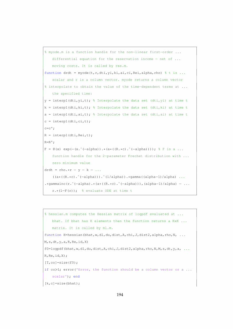
% myode.m is a function handle for the non−linear first−order ...

differential equation for the reservation income − net of ...

moving costs. It is called by res.m.

function drdt = myode(t,r,dti,yi,ki,ai,ci,Rei,alpha,rho) % t is ...

scalar and r is a column vector. myode returns a column vector

% interpolate to obtain the value of the time−dependent terms at ...

the specified time:

y = interp1(dti,yi,t); % Interpolate the data set (dti,yi) at time t

k = interp1(dti,ki,t); % Interpolate the data set (dti,ki) at time t

a = interp1(dti,ai,t); % Interpolate the data set (dti,ai) at time t

c = interp1(dti,ci,t);

c=c';

R = interp1(dti,Rei,t);

R=R';

F = @(x) exp(−(x.ˆ(−alpha)).*(a*((R.*c).ˆ(−alpha)))); % F is a ...

function handle for the 2−parameter Frechet distribution with ...

zero minimum value

drdt = rho.*r − y − k − ...

((a*((R.*c).ˆ(−alpha))).ˆ(1/alpha)).*gamma((alpha−1)/alpha) ...

.*gammainc(r.ˆ(−alpha).*(a*((R.*c).ˆ(−alpha))),(alpha−1)/alpha) − ...

r.*(1−F(r)); % evaluate ODE at time t

% hessian.m computes the Hessian matrix of logpdf evaluated at ...

bhat. If bhat has K elements then the function returns a KxK ...

matrix. It is called by ml.m.

function H=hessian(bhat,w,dl,du,dist,A,chi,J,dist2,alpha,rho,N, ...

M,s,dt,y,a,R,Re,id,X)

f0=logpdf(bhat,w,dl,du,dist,A,chi,J,dist2,alpha,rho,N,M,s,dt,y,a, ...

R,Re,id,X);

[T,co]=size(f0);

if co>1; error('Error, the function should be a column vector or a ...

scalar'); end

[k,c]=size(bhat);

194

if k<c,

bhat=bhat';

end

k=size(bhat,1); % number of parameters wrt which one should compute ...

gradient

h=0.00001; % a small number

H=zeros(k,k); % will contain the Hessian

e=eye(k);

h2=h/2;

for ii=1:k;

if bhat(ii)>100; % if argument is big enough, compute ...

relative number

x0P= bhat.*( ones(k,1) + e(:,ii) *h2 );

x0N= bhat.*( ones(k,1) − e(:,ii) *h2 );

Deltaii = bhat(ii)*h;

else

x0P = bhat + e(:,ii) *h2;

x0N = bhat − e(:,ii) *h2;

Deltaii = h;

end

for jj=1:ii

if bhat(jj)>100; % if argument is big enough, compute ...

relative number

x0PP = x0P .* ( ones(k,1) + e(:,jj) *h2 );

x0PN = x0P .* ( ones(k,1) − e(:,jj) *h2 );

x0NP = x0N .* ( ones(k,1) + e(:,jj) *h2 );

x0NN = x0N .* ( ones(k,1) − e(:,jj) *h2 );

Delta = Deltaii*bhat(jj)*h;

else

x0PP = x0P + e(:,jj) *h2;

x0PN = x0P − e(:,jj) *h2;

x0NP = x0N + e(:,jj) *h2;

x0NN = x0N − e(:,jj) *h2;

195

Delta = Deltaii*h;

end

fPP = logpdf(x0PP,w,dl,du,dist,A,chi,J,dist2,alpha,rho, ...

N,M,s,dt,y,a,R,Re,id,X); % forward,forward

fPN = logpdf(x0PN,w,dl,du,dist,A,chi,J,dist2,alpha,rho, ...

N,M,s,dt,y,a,R,Re,id,X); % forward,backward

fNP = logpdf(x0NP,w,dl,du,dist,A,chi,J,dist2,alpha,rho, ...

N,M,s,dt,y,a,R,Re,id,X); % backward,forward

fNN = logpdf(x0NN,w,dl,du,dist,A,chi,J,dist2,alpha,rho, ...

N,M,s,dt,y,a,R,Re,id,X); % backward,backward

H(ii,jj)=(sum(fPP)−sum(fPN)−sum(fNP)+sum(fNN))/Delta;

H(jj,ii)=H(ii,jj);

end

end

% gradp.m computes the gradient of f evaluated at bhat. It uses ...

forward gradients and adjusts for differently scaled x by ...

taking percentage increments. It is called by ml.m.

function g=gradp(bhat,w,dl,du,dist,A,chi,J,dist2,alpha,rho,N, ...

M,s,dt,y,a,R,Re,id,X,n)

f0=logpdfi(bhat,w,dl,du,dist,A,chi,J,dist2,alpha,rho,N,M,s,dt,y,a, ...

R,Re,id,X);

if size(bhat,2)>size(bhat,1)

bhat=bhat'; % bhat needs to be a column vector

end

p=size(bhat,1); % number of parameters wrt which one should compute ...

gradient

h=0.0000001; % some small number

G=zeros(N,p); % will contain the gradient for the N observations

e=eye(p);

for j=1:p;

196

if bhat(j)>1; % if argument is big enough, compute relative number

f1=logpdfi(bhat.*(ones(p,1) + e(:,j)*h),w,dl,du,dist, ...

A,chi,J,dist2,alpha,rho,N,M,s,dt,y,a,R,Re,id,X);

G(:,j)=(f1−f0)/(bhat(j)*h);

else

f1=logpdfi(bhat + e(:,j)*h,w,dl,du,dist,A,chi,J,dist2, ...

alpha,rho,N,M,s,dt,y,a,R,Re,id,X);

G(:,j)=(f1−f0)/h;

end

end

V = max(n); % number of clusters (individuals)

g=zeros(V,p); % will contain the gradient for the V clusters

v = 1; % v indexes clusters (individuals)

q = 1;

while v < V;

mel = sum(n(:)==v); % number of spells for individual v

g(v,:) = sum(G(q:q+mel−1,:),1); % sum gradients within cluster

q = q+mel;

v = v+1;

end

197