Embed Size (px)
Citation preview

Essays on the Industrial Organization of HealthCare Markets
by
Eli Sellinger-Liebman
Department of EconomicsDuke University
Date:Approved:
Allan Collard-Wexler, Supervisor
Attila Ambrus
David Ridley
Jimmy Roberts
Donald Taylor
Dissertation submitted in partial fulfillment of the requirements for the degree ofDoctor of Philosophy in the Department of Economics
in the Graduate School of Duke University2017

Abstract
Essays on the Industrial Organization of Health Care Markets
by
Eli Sellinger-Liebman
Department of EconomicsDuke University
Date:Approved:
Allan Collard-Wexler, Supervisor
Attila Ambrus
David Ridley
Jimmy Roberts
Donald Taylor
An abstract of a dissertation submitted in partial fulfillment of the requirements forthe degree of Doctor of Philosophy in the Department of Economics
in the Graduate School of Duke University2017

Copyright c© 2017 by Eli Sellinger-LiebmanAll rights reserved except the rights granted by the
Creative Commons Attribution-Noncommercial Licence

Abstract
This dissertation examines three separate issues of the industrial organization of
health care markets. There are a number of features which differentiate health care
from other industries. In my dissertation I examine three features: (1) the role of
government setting prices, (2) the use of networks, or refusing to contract in order
to gain bargaining leverage and, (3) adverse selection.
The second chapter explores the role of government reimbursement in providing
incentives for manufacturing quality. To do this my coauthors and I examine whether
the Medicare Modernization Act (2003), which reduced the reimbursement for physi-
cians for certain drugs, affected the amount of drug shortages. We hypothesize that
as these drugs become less profitable, there is less incentive for manufacturers to in-
vest in the reliability of their manufacturing lines, double source ingredients or build
newer facilities. This would lead to more drug shortages. We use a difference-in-
difference approach and find evidence that more drug shortages are correlated with
drugs that are most affected by the policy change.
The third chapter explores the common story that insurance companies exclude
hospitals from their networks to gain bargaining leverage in contract negotiations.
To do this, I propose a novel model of price formation in a bilateral oligopoly set-
ting where the networks are endogenous. The endogeneity of its network allows the
insurer to threaten to exclude hospitals. I show that exclusion is an equilibrium
outcome of the model; the insurer offsets the loss of premiums from a less valuable
iv
network by reimbursing hospitals less. I then estimate this model using data from
the Colorado All-Payer Claims Database. I find, using a counterfactual analysis,
that restricting insurers’ ability to exclude would lead to 20 percent higher prices
negotiated between hospitals and insurers, which is mostly passed through to con-
sumers as higher premiums. This worsens consumer surplus as the value of broader
networks is offset by the higher premiums consumers face.
The fourth chapter incorporates adverse selection into the standard model of
price formation in hospital markets. A typical merger analysis seeks to quantify the
anti-competitive effects of a merger. For example, do hospitals gain more power by
merging? However, in a market with adverse selection, if a merger leads to hospitals
to negotiate higher prices, this may lead to higher premiums, and the healthiest
consumers being priced out of the market. This may raise premiums even more.
Therefore, a hospital merger may also have welfare consequences through the channel
of adverse selection. This suggests that a merger analysis which focuses solely on
competitive effects may underestimate the welfare consequences of a merger.
v

Contents
Abstract iv
List of Tables ix
List of Figures xi
Acknowledgements xii
1 Introduction 1
2 The Role of Government Reimbursement in Drug Shortages 5
2.1 Background . . . . . . . . . . . . . . . . . . . . . . . . . . . . . . . . 7
2.1.1 Manufacturing . . . . . . . . . . . . . . . . . . . . . . . . . . 9
2.1.2 Reimbursement Changes . . . . . . . . . . . . . . . . . . . . . 9
2.1.3 Surplus for Providers and Manufacturers . . . . . . . . . . . . 14
2.2 Theory . . . . . . . . . . . . . . . . . . . . . . . . . . . . . . . . . . . 14
2.3 Data . . . . . . . . . . . . . . . . . . . . . . . . . . . . . . . . . . . . 18
2.3.1 Medicare Market Share (MMS) . . . . . . . . . . . . . . . . . 22
2.3.2 Sample Definition . . . . . . . . . . . . . . . . . . . . . . . . . 24
2.4 Empirical Analysis . . . . . . . . . . . . . . . . . . . . . . . . . . . . 25
2.4.1 Shortages Conditional on Medicare Market Share . . . . . . . 26
2.4.2 Shortages Conditional on Reimbursements to Health Providers 28
2.4.3 Shortages Conditional on Manufacturer’s Prices . . . . . . . . 29
2.4.4 Correlation in Payments to Providers and Manufacturers . . . 30
vi

2.5 Results . . . . . . . . . . . . . . . . . . . . . . . . . . . . . . . . . . . 31
2.5.1 Results for Shortages Conditional on Medicare Market Share . 33
2.5.2 Results for Shortages Conditional on Reimbursements to HealthProviders . . . . . . . . . . . . . . . . . . . . . . . . . . . . . 36
2.5.3 Results for Shortages Conditional on Manufacturers’ Prices . . 36
2.5.4 Results for Correlation in Payments to Providers and Manu-facturers . . . . . . . . . . . . . . . . . . . . . . . . . . . . . . 37
2.6 Discussion . . . . . . . . . . . . . . . . . . . . . . . . . . . . . . . . . 37
2.7 Conclusion . . . . . . . . . . . . . . . . . . . . . . . . . . . . . . . . . 40
3 Bargaining in Markets with Exclusion:An Analysis of Health Insurance Networks 50
3.1 Literature Review . . . . . . . . . . . . . . . . . . . . . . . . . . . . . 55
3.1.1 Reduced-Form Estimates of Savings from Managed Care . . . 55
3.1.2 Theory on Exclusion and Bargaining Over Networks . . . . . . 56
3.1.3 Nash-in-Nash Bargaining Model . . . . . . . . . . . . . . . . . 57
3.1.4 Other Mechanisms for Savings from Narrow Networks . . . . . 59
3.2 Data . . . . . . . . . . . . . . . . . . . . . . . . . . . . . . . . . . . . 60
3.3 Reduced-Form Evidence . . . . . . . . . . . . . . . . . . . . . . . . . 64
3.4 Stylized Bargaining Model . . . . . . . . . . . . . . . . . . . . . . . . 68
3.4.1 Fundamentals . . . . . . . . . . . . . . . . . . . . . . . . . . . 70
3.4.2 Equilibrium Strategy Profile . . . . . . . . . . . . . . . . . . . 73
3.4.3 Determining Continuation Values . . . . . . . . . . . . . . . . 74
3.4.4 Bargaining Results . . . . . . . . . . . . . . . . . . . . . . . . 75
3.5 Structural Model and Estimation . . . . . . . . . . . . . . . . . . . . 79
3.5.1 Defining Surplus . . . . . . . . . . . . . . . . . . . . . . . . . 80
3.5.2 Stage 1 - Providers and Insurers Bargain over Prices and theNetwork . . . . . . . . . . . . . . . . . . . . . . . . . . . . . . 85
vii

3.6 Results . . . . . . . . . . . . . . . . . . . . . . . . . . . . . . . . . . . 92
3.6.1 Demand Estimation Results . . . . . . . . . . . . . . . . . . . 92
3.6.2 Bargaining Estimation Results . . . . . . . . . . . . . . . . . . 94
3.7 Counterfactuals . . . . . . . . . . . . . . . . . . . . . . . . . . . . . . 95
3.8 Limitations and Extensions . . . . . . . . . . . . . . . . . . . . . . . 97
3.9 Conclusion . . . . . . . . . . . . . . . . . . . . . . . . . . . . . . . . . 98
4 Hospital-Insurer Bargaining in Selection Markets 108
4.1 Introduction . . . . . . . . . . . . . . . . . . . . . . . . . . . . . . . . 108
4.2 Literature Review . . . . . . . . . . . . . . . . . . . . . . . . . . . . . 110
4.3 Theory . . . . . . . . . . . . . . . . . . . . . . . . . . . . . . . . . . . 111
4.3.1 No Selection Case . . . . . . . . . . . . . . . . . . . . . . . . . 112
4.3.2 Incorporating Adverse Selection . . . . . . . . . . . . . . . . . 112
4.4 Structural Model . . . . . . . . . . . . . . . . . . . . . . . . . . . . . 114
4.5 Conclusion . . . . . . . . . . . . . . . . . . . . . . . . . . . . . . . . . 118
A Chapter 2 Appendix 120
B Chapter 3 Appendix 123
B.1 Data Appendix . . . . . . . . . . . . . . . . . . . . . . . . . . . . . . 123
B.2 Complete Bargaining Model . . . . . . . . . . . . . . . . . . . . . . . 124
B.2.1 Fundamentals . . . . . . . . . . . . . . . . . . . . . . . . . . . 125
B.2.2 Equilibrium Strategy Profile . . . . . . . . . . . . . . . . . . . 130
B.2.3 Determining Continuation Values . . . . . . . . . . . . . . . . 132
B.2.4 Bargaining Results . . . . . . . . . . . . . . . . . . . . . . . . 135
B.3 Defining Acceptable Replacement Hospitals . . . . . . . . . . . . . . 138
Bibliography 140
Biography 148
viii

List of Tables
2.1 Descriptive Statistics . . . . . . . . . . . . . . . . . . . . . . . . . . . 41
2.2 OLS and IV Estimates of the Effect of MMS on Shortage Days . . . . 42
2.3 First Stage - MarketScan MMS on IMS MMS . . . . . . . . . . . . . 43
2.4 First Stage - Predicted MMS � Year ¥ 2005 . . . . . . . . . . . . . . 43
2.5 Robustness Check: Different Patent Definitions . . . . . . . . . . . . 44
2.6 Falsification Test Using 2003 as Regulation Year . . . . . . . . . . . . 45
2.7 OLS and IV Year By Year Coefficient Estimates . . . . . . . . . . . . 46
2.8 The Effect of the Reimbursement Change and Patent Status on Short-age Days . . . . . . . . . . . . . . . . . . . . . . . . . . . . . . . . . . 47
2.9 OLS and Lagged OLS Estimates of Medicare Reimbursement Effecton Shortages . . . . . . . . . . . . . . . . . . . . . . . . . . . . . . . . 48
2.10 OLS and Lagged OLS Estimates of Manufacturer Price Effect onShortages . . . . . . . . . . . . . . . . . . . . . . . . . . . . . . . . . 48
2.11 Effect of Medicare Reimbursement on Price to Manufacturers . . . . . 49
3.1 Summary Statistics . . . . . . . . . . . . . . . . . . . . . . . . . . . . 99
3.2 Correlations between Network Size and Prices . . . . . . . . . . . . . 100
3.3 Correlations between Network Size and Prices . . . . . . . . . . . . . 100
3.4 Correlations between Network Size and Premiums . . . . . . . . . . . 101
3.5 Demand for Hospitals . . . . . . . . . . . . . . . . . . . . . . . . . . . 102
3.6 Prevalence of Condition Categories . . . . . . . . . . . . . . . . . . . 103
3.7 Prevalence of Conditions by Age . . . . . . . . . . . . . . . . . . . . . 103
ix

3.8 Summary Statistics for WTP for Networks . . . . . . . . . . . . . . . 104
3.9 Demand for Networks . . . . . . . . . . . . . . . . . . . . . . . . . . . 104
3.10 Premium Sensitivity . . . . . . . . . . . . . . . . . . . . . . . . . . . 105
3.11 Hospital-Specific Bargaining Parameters, ρHj . . . . . . . . . . . . . . 105
3.12 Insurer-Specific Bargaining Parameters, ρIr . . . . . . . . . . . . . . . 106
3.13 Insurer-Specific Exclusion Parameters θr . . . . . . . . . . . . . . . . 106
3.14 Counterfactual Negotiated Prices . . . . . . . . . . . . . . . . . . . . 107
A.2 OLS and IV Estimates of the Effect of MMS on Shortage Days . . . . 121
A.3 First Stage - MarketScan MMS on IMS MMS . . . . . . . . . . . . . 122
A.4 First Stage - Predicted MMS � Year ¥ 2005 . . . . . . . . . . . . . . 122
x

List of Figures
2.1 Shortage Days per Year for Sterile Injectable and Other Drugs . . . . 6
2.2 Supply Chain for a Drug Administered by a Provider . . . . . . . . . 8
2.3 Medicare Part B Reimbursement Levels and Changes for Off-PatentDrugs . . . . . . . . . . . . . . . . . . . . . . . . . . . . . . . . . . . 11
2.4 Revenue per Year for Medicare and the Entire Market . . . . . . . . . 12
2.5 Shortage Frequency as a Function of the Model’s Parameters . . . . . 19
2.6 Prices for Generic Injectable Drugs . . . . . . . . . . . . . . . . . . . 31
3.1 Insurer’s t � 0 expected value by network size. . . . . . . . . . . . . . 78
4.1 Demand and Average Cost Curve Under Adverse Selection . . . . . . 113
xi

Acknowledgements
I would like to thank my advisor, Allan Collard-Wexler, and the remainder of my
committee Attila Ambrus, David Ridley, Jimmy Roberts, and Don Taylor for many
excellent comments and suggestions.
For chapter 2, I would like to thank my co-authors Ali Yurukoglu and David
Ridley. Frank Sloan’s comments as a referee on my second year paper helped to
improve this paper.
For chapter 3, I would like to thank the Duke Public/IO lunch group, the Duke
Micro Theory lunch group, and conference participants at the 2016 American Society
of Health Economists conference (Philadelphia). Allan Collard-Wexler, Attila Am-
brus and Ali Yurukoglu provided excellent comments throughout and I am grateful
for the time you took to read my drafts. Matt Grennan provided a number of cru-
cial insights. Finally, Curtis Taylor and the Duke Economics Department for data
acquisition funding, and the Duke Graduate School for summer research support.
For chapter 4, I would like to thank my co-author Matthew Panhans.
I would also like to thank Matthew Panhans for many helpful discussions and
generosity. Margaux Luflade for many excellent discussions, support, and encour-
agement. Also, Ana Aizcorbe and Abe Dunn deserve credit as role models, demon-
strating the research process to me, and teaching me to not be afraid of answering
hard questions.
xii

1
Introduction
There are a number of features that differentiate health care markets from the canon-
ical models in economics. In each of the chapters, I model the market as having a
vertical structure, i.e. consumers are administered injectable drugs through a physi-
cians, while physician purchase those drugs from their manufacturer. Furthermore,
these are markets where both sides of the market may be best considered to be an
oligopoly. In chapter 2, the market has many physicians or hospitals downstream
and many drug manufacturers upstream. In chapters 3 and 4, markets have many
hospitals upstream and many insurers downstream. This market arrangement is re-
ferred to as having a bilateral oligopoly. The difficulty of these types of market is
that theory is less precise about how prices are formed, but without considering the
vertical structure of the markets, it would be difficult to capture the mechanisms I
focus on in these chapters.
Furthermore, each chapter examines specific features of health care markets in
the United States, which are less common in other markets. One interesting feature
of the health care industry in the United States is the role of government. Chap-
ter 2 takes into account the role the government plays in setting prices. Chapter 3
1

examines the use of excluding firms from insurance networks. Insurers use this strat-
egy with physicians, hospitals, and increasingly with pharmacies. Finally, chapter
4 incorporates adverse selection into the cutting edge model of bilateral oligopoly,
showing how adverse selection may play an important role in anti-trust policy.
Chapter 2 is the first paper in the economics literature look at drug shortages.
A drug shortage in our data is a complaint that a physician or hospital is unable to
purchase a drug. In other words, the manufacturer is unable to meet demand. The
drugs that have shortages are injectable drugs that are administred by physicians
or hospitals, like chemotherapy, anathesia or vaccines. These drugs are expensive
and complicated to make, because they are injectable, and because they are injected
directly into your blood stream they have to be sterile.
For certain patients, physicians or hospitals are reimbursed by private insurance
and for some patients physicians and hospitals are reimbursed by Medicare. In this
case, the prices that physicians and hospitals receive may affect an upstream drug
manufacturers’ ability to negotiate their own prices. Therefore, government price
setting in the downstream market can affect the upstream prices. We hypothesize
that a policy change that affected reimbursement to physicians and hospitals reduced
the prices that drug manufacturers are able to negotiate. This makes those drugs
less profitable, reducing the incentive for manufacturers to invest in the reliability of
their manufacturing lines, double source ingredients or build newer facilities. This
leads to shortages as manufacturers have to shut down lines due to quality concerns.
We use a difference-in-difference approach to test this hypothesis. The policy
change we exploit is the Medicare Modernization Act reduced how much Medicare
reimbursed physicians and hospitals. Since Medicare only covers the elderly, we argue
that drugs which treat conditions that are more likely for the elderly to have should
be differentially effected. The idea is that drugs which are purchased by the elderly
would see their revenue reduced the most, so they should see the largest increases in
2
shortages. We find evidence that this is the case. And that raises important questions
about how the government should reimburse drugs. The optimal reimbursement for
a generic drug might not be marginal cost because that will lead to shortages as
firms in the market are unwilling to pay the fixed costs as maintance requires it.
Chapter 3 explores the common story among the health policy community that in-
surance companies exclude hospitals from their networks to gain bargaining leverage
in contract negotiations. The challenge is that modeling bargaining leverage requires
modeling the market as a bilateral oligopoly, thinking of either side as a price-setter
gives all bargaining leverage to one side of the market. However, the cutting edge
model of bilateral oligopoly, developed in Crawford and Yurukoglu (2012a), treats
the networks as exogenous and exclusion must be due to other reasons. My job
market paper builds on this literature by incorporating an insurers ability to exclude
hospitals as a strategy.
I develop a new model of bargaining between many insurers and many hospitals.
While the literature on exclusive dealing does not detail this mechanism as a reason
for exclusion, I show that it can be a profitable strategy for insurers to exclude
hospitals from their network in order to gain bargaining leverage in their negotiations
with hospitals. Even though an insurer loses some ability to set high premiums,
since it has a lower quality network, it can make up for this by paying lower prices
to hospitals.
I apply this new model of the insurer-hospital market to examine regulations
around networks. Regulators worry that patients lack information about which con-
ditions they will get in the future; without knowing what conditions they will have
in the coming year, they may not check whether high quality providers are available
in each specialty. However, these plans are popular because they charge lower pre-
miums. These lower premiums are due to reduced markups to hospitals since they
lose bargaining power. Therefore, there is a tradeoff for the policy maker, on one
3

hand they reduce deadweight loss due to insurers not contracting with all hospitals,
but they create deadweight loss due to hospitals gaining markup.
I empirically evaluate this tradeoff using data from the Colorado All-Payer Claims
Database. I find, using a counterfactual analysis, that restricting insurers’ ability to
exclude would lead to 20 percent higher prices negotiated between hospitals and
insurers, which is mostly passed through to consumers as higher premiums. This
worsens consumer surplus as the value of broader networks is offset by the higher
premiums consumers face.
Chapter 4 incorporates adverse selection into the standard model of price for-
mation in hospital markets. A typical merger analysis seeks to quantify the anti-
competitive effects of a merger. For example, do hospitals gain more power by
merging? However, in a market with adverse selection, if a merger leads to hospi-
tals to negotiate higher prices, this may lead to higher premiums, and the healthiest
consumers being priced out of the market. This may raise premiums even more.
Therefore, a hospital merger may also have welfare consequences through the chan-
nel of adverse selection. This suggests that a merger analysis which focuses solely on
competitive effects may underestimate the welfare consequences of a merger.
4

2
The Role of Government Reimbursement in DrugShortages
Beginning in the mid-2000s, the incidence of drug shortages rose, especially for
generic injectable drugs (Figure 2.1).1 Examples include drugs used in chemotherapy,
antibiotics and anesthesia, as well as injectable electrolytes and vitamins. Shortages
cause doctors and patients to seek alternatives that are unfamiliar or inferior. When
substitutes are unacceptable, doctors and patients delay or forego treatment.2 Most
of the drugs that experienced shortages were off patent and had previously been
readily available.3
We investigate how declining reimbursement affected the rise of shortages of ster-
1 This chapter is reproduced with permission of the American Economic Journal: Economic Policy.Copyright American Economic Association.
2 Drug shortages can harm patients, increase costs, and delay clinical trials for new therapies(American Society of Clinical Oncology (2011), American Society of Hematology (2011), AmericanSociety of Anesthesiologists (2010)). Because of shortages of mechlorethamine, doctors used a sub-stitute (cyclophosphamide), resulting in higher relapse rates for children with Hodgkin’s lymphoma(Metzger et al., 2012).
3 See Kaakeh et al. (2011) regarding the incidence of shortages. See Panel (2009); Rosoff et al.(2012) regarding guidelines for dealing with shortages. See Conti and Berndt (2013) and Ridleyet al. (2016) regarding shortages of cancer drugs and vaccines, respectively.
5

020
,000
40,0
0060
,000
Shor
tage
Mol
ecul
e-D
ays
per Y
ear
2001 2002 2003 2004 2005 2006 2007 2008 2009 2010 2011 2012
Sterile Injectables Other Drugs
Figure 2.1: Shortage Days per Year for Sterile Injectable and Other Drugs
Source: University of Utah Drug Information Service
ile injectable drugs in the United States. One such change was the Medicare Modern-
ization Act (MMA) which reduced Medicare reimbursement for health care providers
that administer these drugs.4 We begin by specifying a theoretical model of how re-
imbursement policy and market size influence shortages. Our model implies that the
decision by manufacturers to invest in reliability and quality depends on the expected
returns.5 If the returns are sufficiently high, then manufacturers will dual source in-
gredients, perform monitoring and maintenance on manufacturing lines, and build
newer or more robust manufacturing lines. These actions can reduce the likelihood
of shortages.
Consistent with the theoretical model, the empirical results suggest supply-side
4 Duggan and Scott Morton (2010) examine the effect of the MMA on prices in the retail market.Furthermore, Jacobson et al. (2010) examine the effect of the MMA on treatment patterns byoncologists.
5 See also Woodcock and Wosinska (2012).
6

responses to decreasing margins. We begin by showing that drugs with greater ex-
posure to the policy change experienced greater increases in shortages. Exposure to
the policy change is measured using the Medicare market share (MMS) – the fraction
of a drug’s revenue that comes from Medicare fee for service patients.6 Consistent
with our theoretical model, we find that drugs for which reimbursements fell more
after the policy change had greater increases in shortages. The results hold whether
measuring reimbursement from Medicare to health providers (which the policy di-
rectly affected, but which only indirectly affects profit) or a manufacturers’ average
revenue per dose (which the policy only indirectly affected, but which directly affects
profit).
The median drop in reimbursement from Medicare to providers for generic sterile
injectable drugs after the policy change was about 50 percent. We estimate that a 50
percent drop in reimbursement to providers would increase the number of expected
shortage days by 16 per year from a mean of 60.
2.1 Background
The pharmaceutical industry is highly regulated. Approval by the U.S. Food and
Drug Administration (FDA) is required before manufacturers may market branded
or generic prescription drugs. A manufacturer of a branded drug must demonstrate
efficacy and safety compared to a placebo. Likewise, a manufacturer of a generic
drug must demonstrate that its generic drug is pharmaceutically equivalent to the
branded drug and that the manufacturing process follows good manufacturing prac-
tices including ensuring sterility for injectable dosage forms (Scott Morton, 1999).
Injectable drug sales totaled $83 billion dollars and 3.7 billion units in 2010, ac-
cording to our IMS Health data sample (which we describe in section 2.3). Injectable
6 Our MMS measure is similar to the Medicare market share measure used by Duggan andScott Morton (2010) who study the effect of introducing Medicare Part D.
7
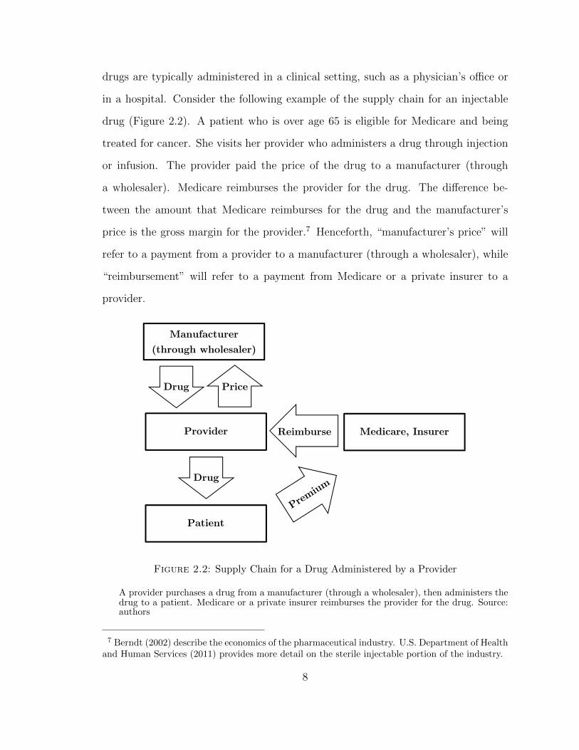
drugs are typically administered in a clinical setting, such as a physician’s office or
in a hospital. Consider the following example of the supply chain for an injectable
drug (Figure 2.2). A patient who is over age 65 is eligible for Medicare and being
treated for cancer. She visits her provider who administers a drug through injection
or infusion. The provider paid the price of the drug to a manufacturer (through
a wholesaler). Medicare reimburses the provider for the drug. The difference be-
tween the amount that Medicare reimburses for the drug and the manufacturer’s
price is the gross margin for the provider.7 Henceforth, “manufacturer’s price” will
refer to a payment from a provider to a manufacturer (through a wholesaler), while
“reimbursement” will refer to a payment from Medicare or a private insurer to a
provider.
Manufacturer
(through wholesaler)
Medicare, Insurer
Patient
Provider
Drug Price
Reimburse
Drug
Figure 2.2: Supply Chain for a Drug Administered by a Provider
A provider purchases a drug from a manufacturer (through a wholesaler), then administers thedrug to a patient. Medicare or a private insurer reimburses the provider for the drug. Source:authors
7 Berndt (2002) describe the economics of the pharmaceutical industry. U.S. Department of Healthand Human Services (2011) provides more detail on the sterile injectable portion of the industry.
8

2.1.1 Manufacturing
Sterility is critical for injectable drugs because they are administered intravenously,
intramuscularly, or subcutaneously rather than passing through the gastrointestinal
tract. Manufacturing lines must not be contaminated by bacteria, fungus, or mold
which causes delays to clean up the problem. In some cases, remediation is so
costly relative to expected profit that the manufacturer stops producing the drug.
Also, shortages might occur due to disruptions to supplies of active pharmaceutical
ingredients.
A typical generic injectable drug is made by three to four manufacturers out of
seven major generic injectable manufacturers selling in the United States.8 Once
one manufacturer stops producing, it falls to the other manufacturers to make up
the supply difference. However, the other manufacturers might have been affected
by the same supply shock, might not find it profitable to produce more units of the
drug given capacity constraints, or might not be licensed to produce the drug.
2.1.2 Reimbursement Changes
Medicare provides health insurance for seniors and the disabled. Medicare covers
hospitals and hospice (Medicare Part A), as well as physician visits and outpatient
services (Medicare Part B). Under Part B, physicians are reimbursed when they ad-
minister a drug (often a sterile injectable). Until 2005, Medicare Part B reimbursed
providers for drugs based on Average Wholesale Price (AWP). However, AWP was a
list price, not an actual average price. According to the Medicare Payment Advisory
Commission (2003): “[AWP] does not correspond to any transaction price... AWP
has never been defined by statute or regulation. Individual AWPs are compiled in
compendia like the Red Book and First Databank”. As such, the AWP was often
8 APP-Fresenius, Bedford-Ben Venue, Daiichi Sankyo, Hospira, Sandoz, Teva, and West-Ward.Several of these manufacturers, as well as smaller manufacturers, experienced shortages.
9

substantially higher than the actual transaction price. The Medicare Payment Ad-
visory Commission (2003) cited some dramatic examples: Vincasar, a chemotherapy
drug, had an AWP of $740, while being sold to physicians for $7.50.9 Berndt (2005)
provides a detailed history of AWP. By raising AWP, manufacturers could raise the
profitability of providers that chose their drug. However, the threat of litigation and
new regulation probably disciplined AWP.10
In 2003, the Medicare Modernization Act (MMA) (officially known as the Medi-
care Prescription Drug Improvement and Modernization Act of 2003) created the
retail drug benefit known as Medicare Part D and changed reimbursement under
Medicare Part B. In 2004, MMA changed Medicare reimbursement from the pre-
viously used 95 percent of AWP to 85 percent of AWP. Starting January 1, 2005,
Medicare began to reimburse these drugs at 106 percent of the Average Sales Price
(ASP) for the previous two quarters. The ASP is the volume-weighted average price
across all manufacturers of a given drug to all buyers from two quarters prior. The
ASP captures actual transaction prices, including most discounts and rebates. A
study by the Office of Inspector General found that the median percentage differ-
ence between AWP and ASP was 50 percent (Office of Inspector General, 2005).
The change resulted in decreases on the order of 50 percent of reimbursements for
these drugs to providers as seen in Figure 2.3. Furthermore, the policy change clearly
affected the level of reimbursements paid by Medicare as shown in Figure 2.4. There
is a clear drop in revenue paid by Medicare in 2005, followed by below private growth
in Medicare reimbursements. The ASP regime is not a government price control – it
is cost-based reimbursement – but it substantially reduced reimbursements.11
The MMA dramatically reduced reimbursement to providers for many generic
9 AWP was referred to as “Ain’t What’s Paid” (Mullen, 2007).
10 For example, the U.S. Department of Justice sued Abbott for violating the False ClaimsAct by reporting a high AWP for its products, including an intravenous antibiotic. For moreinformation, see https://www.justice.gov/opa/pr/pharmaceutical-manufacturers-pay-4212-million-
10

Figure 2.3: Medicare Part B Reimbursement Levels and Changes for Off-Patent Drugs
The left panel is the unweighted distribution of the reimbursement level, and the right panel isthe unweighted distribution of reimbursement changes. Source: CMS Part B National Summary
drugs. Before the MMA, there was a large spread between the low generic price paid
by providers and the high reimbursement provided by the government and other
payers. After the MMA, reimbursement fell, putting financial stress on providers
who sometimes changed treatment patterns, including changing drug regimens. For
example, some providers changed from carboplatin and paclitaxel to docetaxel (Ja-
cobson et al., 2010). The change also put downward pressure on generic prices.
Hence, generic manufacturers might see profit fall due to changes in both quantity
settle-false-claims-act-cases.
11 ASP is based on the two previous quarters which introduces rigidity into the price mechanism
and might exacerbate the shortage problem. However, ASPs can and do rise by more than 6 percentfrom quarter to quarter in the data, so we conclude that this aspect of the switch to ASP is secondorder compared to the decrease in the realized levels of reimbursements.
11
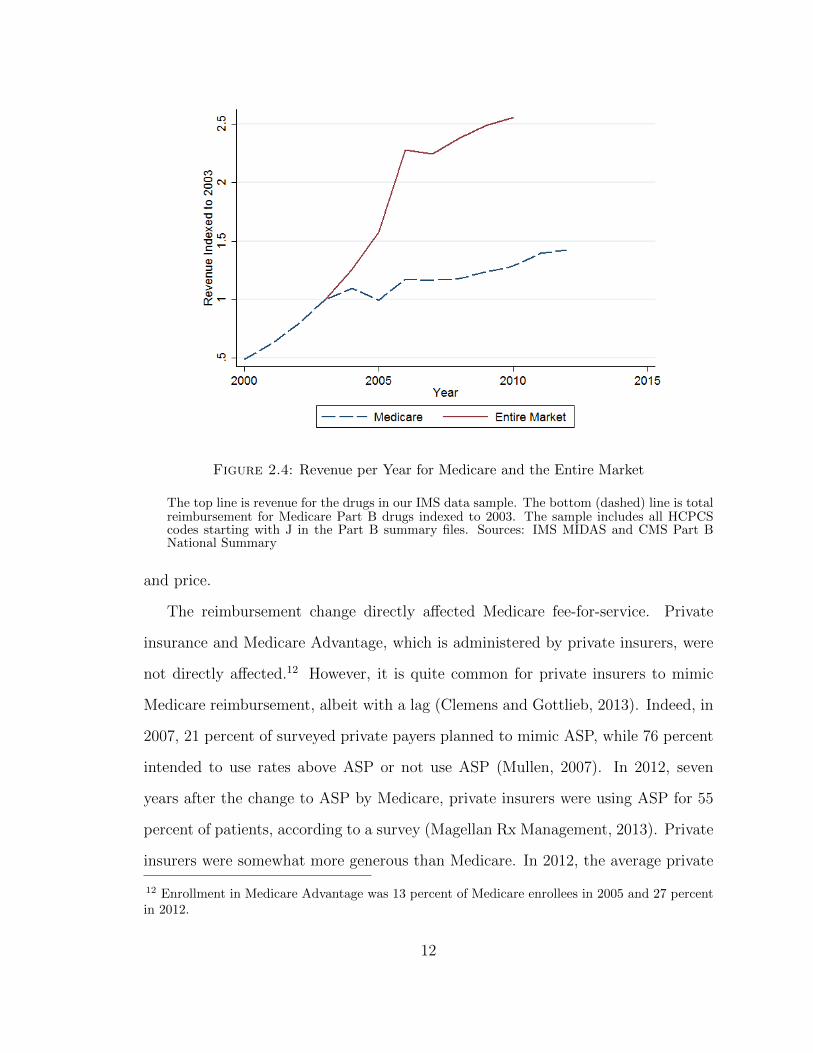
Figure 2.4: Revenue per Year for Medicare and the Entire Market
The top line is revenue for the drugs in our IMS data sample. The bottom (dashed) line is totalreimbursement for Medicare Part B drugs indexed to 2003. The sample includes all HCPCScodes starting with J in the Part B summary files. Sources: IMS MIDAS and CMS Part BNational Summary
and price.
The reimbursement change directly affected Medicare fee-for-service. Private
insurance and Medicare Advantage, which is administered by private insurers, were
not directly affected.12 However, it is quite common for private insurers to mimic
Medicare reimbursement, albeit with a lag (Clemens and Gottlieb, 2013). Indeed, in
2007, 21 percent of surveyed private payers planned to mimic ASP, while 76 percent
intended to use rates above ASP or not use ASP (Mullen, 2007). In 2012, seven
years after the change to ASP by Medicare, private insurers were using ASP for 55
percent of patients, according to a survey (Magellan Rx Management, 2013). Private
insurers were somewhat more generous than Medicare. In 2012, the average private
12 Enrollment in Medicare Advantage was 13 percent of Medicare enrollees in 2005 and 27 percentin 2012.
12

insurance markup over ASP was 18 percent (Academy of Managed Care Pharmacy,
2013, p.48). Hence, while the change from AWP to ASP was immediate for the
Medicare population, it was somewhat more gradual for privately insured patients.
Nevertheless, we can think of it as being caused by government policy, because policy
makers should know that private insurers often imitate Medicare.
The MMA not only affected Medicare Part B reimbursement, but also created
Medicare Part D. Beginning in 2006, Medicare Part D provided prescription drug
insurance to seniors and the disabled for drugs dispensed by pharmacists, drugs which
are disproportionately oral solids (pills and tablets). The introduction of Medicare
Part D might shift demand to oral solids, reducing demand for injectable or infused
drugs. Reductions in demand for injectable or infused drugs would not directly cause
shortages (just the opposite) but in the long run could reduce profit and the incentive
to manufacture a drug.
A second change in reimbursement was the expansion of the Medicaid 340B pro-
gram with more drugs purchased by covered entities. Drug purchases under the 340B
Program account for about 2 percent of all U.S. drug purchases (U.S. Department
of Health and Human Services, 2013, p.311). The program requires that drug man-
ufacturers offer discounts to outpatient facilities that can be classified as safety-net
providers for low-income patients. Because these drugs are offered at a discount,
the growth implies lower revenue for drug manufacturers.13 Our estimates do not
isolate the effect of reduced incentives because of 340B. However, both MMA and
340B reduced incentives because of government policies that affect reimbursement
13 Occasionally, news outlets highlight large price increases for generic drugs. Price increases tendto occur when manufacturers have market power due to exits or acquisitions. Our model (section2.2) predicts higher generic prices when there are fewer manufacturers. However, these large priceincreases for generic drugs are rare. According to Janine Burkett of pharmacy benefits managerExpress Scripts, “Price inflation among a few generic drugs has been in the news lately,” but the“Express Scripts Prescription Price Index shows that, since 2008, the average price of brand drugshas almost doubled, while the average price of generic drugs has been cut roughly in half” (Burkett,2014).
13
and prices.
2.1.3 Surplus for Providers and Manufacturers
Prior to the policy change, reimbursement to providers was typically much higher
than the prices they paid, so both providers and manufacturers could capture (short-
run) surplus. For example, as much as half of an oncologists’ income may have come
from the surplus on drugs. Likewise, branded manufacturers charged prices consid-
erably higher than marginal costs. Even generic manufacturers can charge prices
above marginal costs if fixed costs are large (some sterile injectable manufacturing
requires costly facilities), products are not identical (due to reputation, availability,
and relationships), or long-run equilibrium has not been reached.
The MMA caused providers to be reimbursed less. Furthermore, the reimburse-
ment change compressed the scope of price differentiation for manufacturers. With
Medicare reimbursing at a 6 percent markup on average price, providers that paid
a 7 percent markup on average price would lose money with each purchase. Hence,
both manufacturers and providers likely lost surplus. This is consistent with pre-
vious research on vertical relationships suggesting that large firms on each side of
the market share the surplus (Crawford and Yurukoglu, 2012b; Grennan, 2013a; Ho
and Lee, 2015). Through this channel, the decreased reimbursements to providers
reduced the prices manufacturers receive as well. We investigate the relationship
between provider reimbursement and manufacturer price.
2.2 Theory
We use a model of entry and capacity choice with supply uncertainty to illustrate the
change in production incentives and underlying welfare economics associated with
changing Medicare reimbursement. This class of models has been studied by Carlton
(1978), Deneckere and Peck (1995), and Dana (2001) amongst others. We consider
14
two regimes: list-price reimbursement (AWP) and cost reimbursement (ASP). The
AWP regime features reimbursement at a list price that is higher than what would
normally be the acquisition price of the drug. The ASP regime features reimburse-
ment based on costs to the provider.14
Manufacturers, denoted by i, simultaneously choose capacity levels ki to produce
an identical medicine. After choosing capacities, each manufacturer is hit by a shock
εi which jointly follow a distribution whose CDF is Gp~εq. The new capacity for
manufacturer i is kiεi.
There is a mass of size M of patients which are all willing to pay up to pmax for the
medicine. Of those, Mgov are insured by Medicare. Under cost-based reimbursement
(ASP), if the total capacity in the market after the shocks is less than the market
size M , then the market price of the medicine is equal to pmax. If the total installed
capacity is greater than the market size M , then the price of the good is zero.
pASP p~k,~ε,N,Mq �
"pmax,
°Ni�1 kiεi M
0,°Ni�1 kiεi ¥M
Under AWP reimbursement, the government reimburses hospitals and physicians
for drugs used for Medicare patients at pmax no matter what price the hospital or
physician paid for the medicine.15 The government purchases up to Mgov units at
pmax no matter what total industry capacity turns out to be. Some fraction γ of
that reimbursement rate will go to manufacturers. γ P r0, 1s represents a bargaining
power parameter which is assumed to be the same across manufacturers.
pAWP p~k,~ε,N,M,Mgov, γq �
$&%
pmax,°Ni�1 kiεi M
γpmax,°Ni�1 kiεi ¥M,Medicare
0°Ni�1 kiεi ¥M,Non-Medicare
14 ASP is therefore not a regulated price. However, because ASP is based on data from the twoprevious quarters, it does introduce some frictions into the flexibility of prices if health providersare unwilling to accept a loss on some transactions.
15 The manufacturers only receive the additional payment compared to the ASP regime on Medicarepatients.
15
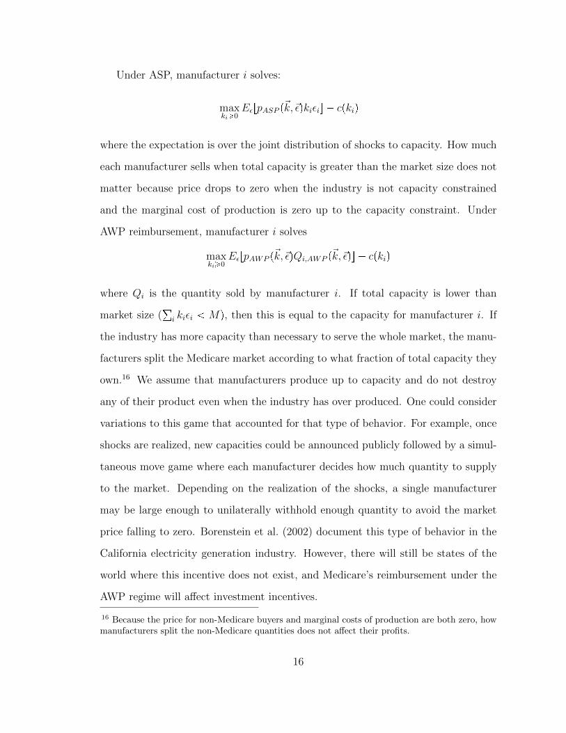
Under ASP, manufacturer i solves:
maxki¥0
EεrpASP p~k,~εqkiεis � cpkiq
where the expectation is over the joint distribution of shocks to capacity. How much
each manufacturer sells when total capacity is greater than the market size does not
matter because price drops to zero when the industry is not capacity constrained
and the marginal cost of production is zero up to the capacity constraint. Under
AWP reimbursement, manufacturer i solves
maxki¥0
EεrpAWP p~k,~εqQi,AWP p~k,~εqs � cpkiq
where Qi is the quantity sold by manufacturer i. If total capacity is lower than
market size (°i kiεi Mq, then this is equal to the capacity for manufacturer i. If
the industry has more capacity than necessary to serve the whole market, the manu-
facturers split the Medicare market according to what fraction of total capacity they
own.16 We assume that manufacturers produce up to capacity and do not destroy
any of their product even when the industry has over produced. One could consider
variations to this game that accounted for that type of behavior. For example, once
shocks are realized, new capacities could be announced publicly followed by a simul-
taneous move game where each manufacturer decides how much quantity to supply
to the market. Depending on the realization of the shocks, a single manufacturer
may be large enough to unilaterally withhold enough quantity to avoid the market
price falling to zero. Borenstein et al. (2002) document this type of behavior in the
California electricity generation industry. However, there will still be states of the
world where this incentive does not exist, and Medicare’s reimbursement under the
AWP regime will affect investment incentives.
16 Because the price for non-Medicare buyers and marginal costs of production are both zero, howmanufacturers split the non-Medicare quantities does not affect their profits.
16

The incentive to invest in capacity is determined by integrating prices over the
joint distribution of ε. Manufacturers must pay an entry cost F to produce and sell
the good. The equilibrium number of firms is given by the maximum number of
firms such that the variable profits of each firm are greater than F.
We find a symmetric Nash equilibrium to the simultaneous capacity choice sub-
game. If the distribution of ε has no mass points, then the symmetric equilibrium
capacity per firm when N firms are producing is the solution to the following equation
under ASP:
EεrpASP pk b eN ,~ε,N, :qεis � c1pkq � 0
where eN is the 1xN vector of ones. Under AWP reimbursement,
Eεr
$&%
pmaxεi,°Nj�1 kεi M
γpmaxMgovεip°N
j�1 kεj�dkq
p°N
j�1 kεjq2,°Nj�1 kεi ¥M
s � c1pkq � 0
We use numerical simulation to show how equilibrium quantities vary with model
parameters.
When γ ¡ 0, equilibrium capacities and average prices are higher under AWP
than ASP. Shortages occur less frequently under AWP than with ASP (Figure 2.5).
Whether total welfare is higher or lower is ambiguous. When a firm enters the indus-
try, it does not capture the full social value of its investment, because competition
drives average price below pmax in some states of the world.17 In the other direction,
the government must raise the funds to pay for the AWP reimbursement, potentially
distorting the decisions in some other area of the economy. Poorly designed AWP
reimbursement can also lead to over entry and over investment in capacity.
17 In this model, conditional on having the socially optimal number of firms, the capacity choicesare socially optimal. This is because price rises to pmax immediately in a shortage. With lessflexible pricing or competitive pressures in shortage states, capacity investment could also be toolow under ASP.
17
The model’s predictions for levels are not surprising. The AWP reimbursement
continues to pay manufacturers for Medicare patients even when the industry over
produces. This implies higher returns to investing in capacity for manufacturers, thus
more total capacity and fewer shortages. The model is useful for empirical analysis
because it predicts a differential impact of the AWP reimbursement depending on
features of the drug. In particular, drugs with lower fixed costs and that serve more
Medicare patients will experience a greater increase in shortages moving from AWP
to acquisition cost-based reimbursement as in ASP.
The contracts negotiated between health providers, wholesalers, and manufac-
turers are more complicated than the simple model put forth here. Contracts often
have non-linearities due to bundled discounts or quantity discounts or other material
clauses. Modeling the nexus of non-linear contracts between strategic agents would
be an important advance to the maintained model. However, it is unlikely that such
a model would change the result that moving from AWP to ASP reimbursement de-
creases incentives to invest in capacity. This is because in such models of the nexus
of linear contracts in other industries (for example Crawford and Yurukoglu (2012b))
the price to the upstream firm, the manufacturer in this paper, will depend strongly
on the surplus created by consumption of the good and competition. Non-linearities
in the contracts may reduce or sharpen this dependence, but there is no theoret-
ical basis that they would overturn the dependence. Since prices and demand for
each product determine the incentives to invest in capacity, the simple model here
captures the first-order determinants of these investment decisions.
2.3 Data
An observation is a drug and year. We refer to a drug as an active ingredient or
a combination of active ingredients. For example, the nutritional product Multiple
Vitamins for Infusion (MVI) is a combination of active ingredients that also ex-
18
0 5 10 15 20 25 300
0.2
0.4
0.6
0.8
1
Conditional on pmax
Sho
rtag
e F
requ
ency
pmax
0 10 20 30 40
0.65
0.7
0.75
0.8
0.85
0.9
0.95
Conditional on Market Size (M)
Sho
rtag
e F
requ
ency
M
0 10 20 30 40 500
0.2
0.4
0.6
0.8
1Conditional on Fixed Cost
Sho
rtag
e F
requ
ency
F0 0.2 0.4 0.6 0.8 1
0.7
0.75
0.8
Conditional on Fraction of Medicare Patients
Sho
rtag
e F
requ
ency
Mgov
/M
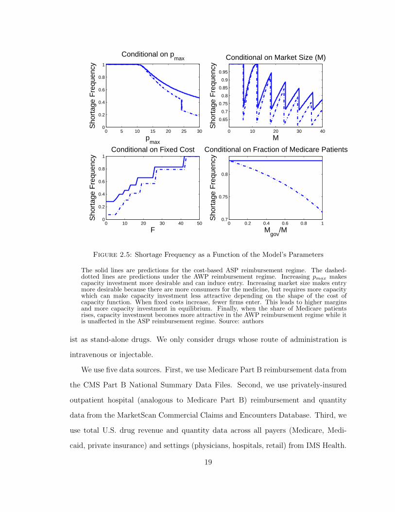
Figure 2.5: Shortage Frequency as a Function of the Model’s Parameters
The solid lines are predictions for the cost-based ASP reimbursement regime. The dashed-dotted lines are predictions under the AWP reimbursement regime. Increasing pmax makescapacity investment more desirable and can induce entry. Increasing market size makes entrymore desirable because there are more consumers for the medicine, but requires more capacitywhich can make capacity investment less attractive depending on the shape of the cost ofcapacity function. When fixed costs increase, fewer firms enter. This leads to higher marginsand more capacity investment in equilibrium. Finally, when the share of Medicare patientsrises, capacity investment becomes more attractive in the AWP reimbursement regime while itis unaffected in the ASP reimbursement regime. Source: authors
ist as stand-alone drugs. We only consider drugs whose route of administration is
intravenous or injectable.
We use five data sources. First, we use Medicare Part B reimbursement data from
the CMS Part B National Summary Data Files. Second, we use privately-insured
outpatient hospital (analogous to Medicare Part B) reimbursement and quantity
data from the MarketScan Commercial Claims and Encounters Database. Third, we
use total U.S. drug revenue and quantity data across all payers (Medicare, Medi-
caid, private insurance) and settings (physicians, hospitals, retail) from IMS Health.
19

Fourth, we use shortage data by molecule and year from the University of Utah Drug
Information Service. Fifth, we use approval dates and the number of manufacturers
per molecule from FDA Orange Book.
First, we use Medicare reimbursements and services given by the CMS Part B
National Summary Data Files. The key variables are the total reimbursements by
Medicare and number of services billed for a Healthcare Common Procedure Coding
System (HCPCS) code and year. Providers use HCPCS codes to bill Medicare and
private payers for procedures. A typical HCPCS code represents one administration
of a drug. For example, the spending by Medicare to a hospital or physician’s office
on a lymphoma patient being treated by chemotherapy agent Doxorubicin once a
month for three months would show up as three services of HCPCS code J9000. The
same drug can have multiple HCPCS codes representing different dosages. We use
data from 2001 to 2012 and adjust reimbursements for inflation to year 2010 dollars.
Second, we use MarketScan Commercial Claims and Encounters database out-
patient files. These data are given at the claims level, but we aggregate to the year
and HCPCS code. The data are not nationally representative, but rather they are a
convenience sample of all claims from large employers and insurance plans. The data
only include enrollees who are under 65. As discussed later, we reweight the data
to match the commercially-insured population in the U.S. We use the years 2001-
2009 to estimate the total non-Medicare spending by year and HCPCS, adjusted for
inflation to year 2010 dollars.
Third, we use IMS MIDAS data for estimates of a drug’s total revenue for the
years 2003 to 2010. We use these data to estimate sales to providers. These data
contain all payers, including private, Medicare, Medicare Advantage, and Medicaid.
Quantities are measured in standard units which can be thought of as doses. For
injectable drugs, a standard unit is often an ampoule or vial. The IMS Health
sales data do not include off-invoice discounts (for example, rebates paid by the
20

manufacturer).
Fourth, we use shortage data from the University of Utah Drug Information
Service (UUDIS) which archives shortages that were reported to the FDA or the
Association of Health System Pharmacists (ASHP) by providers (hospitals or phar-
macists) or manufacturers. In the data, a drug shortage is defined as “a supply issue
that affects how the pharmacy prepares or dispenses a drug product or influences
patient care when prescribers must use an alternative agent” (Fox et al., 2009). A
report of a shortage leads to a response from the FDA and ASHP which usually
leads to rationing and identifying alternative drugs. Furthermore, manufacturers are
contacted to determine which manufacturers, if any, have emergency supplies. This
suggests that manufacturers and the FDA vet the reporting of shortages. Shortages
are specific to a molecule and form (injectable or not) and for the U.S. We also
have information on the dates of shortage start and when they are resolved. We use
shortage data from 2001 to 2012.18
Fifth, we use the Food and Drug Administration Orange Book for the years 2001-
2012 to record how many approved manufacturers of a drug (active ingredient and
route of administration combination) exist in each year, and the number of years since
the earliest approval of a manufacturer of the drug. The FDA Orange Book records
each approved and active manufacturer19 of a given drug in a given year. Because
the analysis is at the drug level, we collapse the observations of a given drug into one
observation per year. The Orange Book does not track biological pharmaceuticals
which are made by a biological process rather than chemical synthesis (e.g., insulin).
These drugs have a more complicated manufacturing process and have been subject
18 An alternative set of shortage data are offered by the FDA. The FDA uses a stricter definition ofa shortage than the UUDIS. However, historical FDA data are not available. The UUDIS measuresof shortages are widely used in the pharmaceutical literature (Fox et al., 2009, 2014).
19 Approved products whose manufacturers no longer actively market the product are listed asdiscontinued in the Orange Book. Our variable measuring the number of manufacturers based onthe Orange Book only counts active manufacturers.
21

to some shortages. We include these drugs but treat them all as single-source, on-
patent drugs during our sample period, because Congress did not create a pathway
for FDA to approve multi-source biologics (biosimilars) until 2010.
2.3.1 Medicare Market Share (MMS)
MMS is the fraction of drug reimbursement from Medicare Part B. We use MMS to
identify which drugs will be more impacted by the Medicare reimbursement change.
Hence, for MMS, cardinality is not particularly important, but ordinality is.
We use two estimates of MMS. For both measures, the numerator is Medicare Part
B sales to physicians. These were the only sales directly affected by the policy change
of switching to ASP reimbursement.20 The two MMS measures vary according to the
denominator: total reimbursement. In the first measure of MMS, the denominator is
the sum of payments to manufacturers for each drug from the IMS database. In the
second measure of MMS, the denominator is the sum of reimbursement for each drug
in the MarketScan database plus the reimbursement in Medicare Part B. The number
of people in the MarketScan data rises from around five million in 2001 to 37 million
in 2009. To create the MarketScan-based estimate of MMS for each year, we scale
the reimbursement by drug as if the sample were nationally representative.21 For
example, suppose there are 10 million individuals in a given year in the MarketScan
data. We scale the reimbursement of each drug by the U.S. population minus the
number of individuals insured by Medicare and/or Medicaid divided by 10 million.
Medicare serves seniors and those with kidney failure. Consistent with this, the
drugs with the highest MMS include inhalants for chronic obstructive pulmonary dis-
ease (a progressive disease caused by smoking), Pegaptanib Sodium (for age-related
20 The Medicare Part B data do not include Medicare Advantage reimbursements. In 2012, Medi-care Advantage accounted for 27 percent of all Medicare enrollees.
21 The data vendors do not claim that the data are nationally representative of the private insur-ance market. However, Dunn et al. (2014) show that reweighting MarketScan data improves therepresentativeness of the sample.
22

macular degeneration), and Triptorelin Pamoate (for prostate cancer). Other drugs
with the highest Medicare share are immunosuppressants used in kidney transplants
which are covered by Medicare for all ages. The drugs with the lowest Medicare
share are those used by a younger population, including Somatrem (human growth
hormone for children), Glatiramer Acetate (for multiple sclerosis), two drugs which
treat hyper-thyroidism, and Urofollitropin (a fertility drug).
While the data used to construct the numerator, reimbursements from Medicare
Part B, represent the population of drugs affected by the policy change, we adjust
our methods to handle imperfect data in the denominator. The IMS measure is not
perfect as it mixes revenues to manufacturers with reimbursement from Medicare
to doctors. Nonetheless, it is a measure of the relative importance of Medicare to
non-Medicare revenues. For example, if revenue to a manufacturer is a constant
fraction of reimbursements to doctors, then this measure would be equal to the true
MMS times a constant. As such, drugs which derive more of their revenue from
Medicare would have relatively higher values of this variable. While not ideal for
interpreting units, the first-order role of this variable is to detect differences in the
change in shortages between drugs which are more or less reliant on Medicare. The
MarketScan measure might have some error because it is only a convenience sample of
the under-65 private insurance market and misses sales to other payers like Medicare
Advantage and Medicaid, as well as sales in other settings like retail or inpatient
hospital.22 As we discuss in section 2.4.1, we use an instrumental variables strategy
to address this measurement error.
22 Missing sales in secondary settings is not a big concern because drugs typically receive most oftheir revenue from one setting. For example, a drug used mainly in retail would typically not havelarge hospital sales.
23

2.3.2 Sample Definition
To combine these data sources, we use each HCPCS code beginning with J (which
indicates drug administration)23 that we observe in the Medicare Part B National
Summary File at any time between 2001 and 2012. For each of the 690 observed
unique HCPCS J codes,24 we determine the relevant active ingredient(s) and route of
administration by examining the HCPCS description and searching the FDA Orange
Book.25 This leaves 616 unique HCPCS J codes whose active ingredient(s) and route
of administration have a match in the FDA Orange Book or are a biologic drug. We
keep drugs whose route of administration is “injection,” leaving 511 HCPCS J codes.
Some drugs have multiple dosages with different HCPCS J codes. The 511 HCPCS
codes correspond to 424 drugs.
Next, we join these data to the Medicare reimbursements from the Part B Na-
tional Summary File by HCPCS code and year. We only keep HCPCS-year observa-
tions which were in the Part B National Summary File. This reduces the sample to
415 drugs. Next, we merge in the MarketScan MMS data by drug.26 There are thirty
additional active ingredients which never manifest in the MarketScan data and are
dropped (leaving 385 drugs in our sample). Many of these drugs are introduced after
2009, which is the last year that we have MarketScan data.
We join these data to two FDA datasets by active ingredient(s) and year. The
Orange Book is the primary FDA data set we use, but it does not include biologics so
we supplement it with data from the drugs@FDA website. We keep all overlapping
observations that either appear in the Orange Book or appear in the drugs@FDA
23 Codes J0000 - J0849 indicate “Drugs other than Chemotherapy” and Codes J8521 to J9000indicate “Chemotherapy Drugs.”
24 The average HCPCS J code contains 15.12 10-digit National Drug Code (NDC) codes.
25 The Orange Book does not cover biologics, vaccines, and some nutritional products.
26 This is a mean across the sample years 2001-2009, so there is one observation for each drug.
24

website with a Biologics License Applications (BLA) number. There were nine drugs
dropped because they neither appeared in the Orange Book nor on the drugs@FDA
website with a BLA.
Next, we join this set of drugs to the IMS MIDAS data by year, active ingre-
dient(s). The matching is done by ingredient name, so it is imperfect. We were
unable to match fifty drugs. Then, sixteen drugs were dropped because their MMS
was greater than one or there was no spending in the IMS data, even if the drugs
were matched. The sample with MarketScan MMS, IMS MMS, and Medicare reim-
bursement information is 310 drugs. We dropped two more drugs because they are
only in the Medicare reimbursement files for one year, which precludes their use in
fixed-effect regressions.
We join this set of drugs to the shortage data by year, active ingredient(s), and
route of administration. If an observation from the sample of drugs does not match
any shortage observation, we record that the drug has no shortages in the period of
the sample. We do not drop any drugs while merging in the shortage data.
The final sample has 308 drugs. This corresponds to 3094 observations. Some
drugs do not have 12 years in our data because they are not in the Part B summary
files for 12 years. Of the 308 drugs in the sample, 102 are always on patent, 111 are
always off patent, and the other 95 switch from on patent to off during the sample
period. The full list of drugs in the sample is in Appendix A.
2.4 Empirical Analysis
We begin by using a difference-in-differences identification strategy to show that
drugs that had greater exposure to the Medicare policy change, measured using
the Medicare market share (MMS), had the greatest increases in shortages (section
2.4.1). Our model suggests that shortages result from reduced manufacturers’ prices,
which we hypothesize results from lower reimbursements to providers. We show
25

that reduced reimbursement to providers, caused by the policy change, is correlated
with increased shortages (section 2.4.2). Then consistent with our prediction that
reduced incentives to manufacturers would lead to more shortages, we show that
lower prices to manufacturers are correlated with more shortages (section 2.4.3).
Following the discussion of vertical markets with bargaining power on each side
(section 2.1.3), we show that lower reimbursements to providers are correlated with
lower manufacturers’ prices (section 2.4.4).
Throughout this section the unit of analysis is a drug and year. We use logged
Medicare market share because the observed distribution of MMS is skewed. Simi-
larly, we use logged prices. To reduce noise in the measure of the Medicare market
share, and because the sample period for the IMS data is shorter than the whole
sample, we average across years to compute one MMS measure for each drug. In the
appendix (Table A.2) we show that the results are robust to using levels rather than
logs of MMS, and using an MMS measure only using years prior to implementation.
2.4.1 Shortages Conditional on Medicare Market Share
First, we test the hypothesis that drugs most affected by the ASP reimbursement,
that is, drugs with a large fraction of their revenues from Medicare Part B, experience
larger increases in shortages. We use a difference-in-differences model where the first
difference is the Medicare (Part B) Market Share (MMSi) of drug i and the second
difference is before and after the policy change (Postt). The specification is motivated
by the assertion that Medicare Market Share is a feature of the diseases that the drug
treats, and is not affected by post-policy changes in the unobservable determinants
of shortage days. The first set of regressions uses a binary pre and post period, where
the treatment was assumed to be applied in 2005, when ASP based pricing went into
effect. Formally, this is modeled as:
26

Shortageit � αi � δt � βPostt � logpMMSiq � γ1pOff Patentitq � εit (2.1)
Shortageit is the number of shortage days in year t. The model includes αi and δt
which are drug and year fixed effects, which control for time-invariant differences
across drugs, including the main effect of logpMMSiq, and a general time trend.
Then, assuming parallel trends without treatment, β is the treatment effect – the
extra shortage days caused by having higher MMS post-regulation. 1pOffPatentitq
is an indicator for whether that drug and year observation was off patent. We classify
a drug as off patent if it has been at least 15 years since the molecule was approved.27
As discussed in (section 2.3.1) we are concerned about error in our measures of
MMS. Under the assumption of classical measurement error, the coefficient on the
interaction term, β, will be attenuated towards zero. We therefore employ instru-
mental variables to deal with the measurement error. Because we ultimately interact
MMS with “post” (the indicator variable for years 2005 and later), we follow the
suggestion in Procedure 21.1 of Wooldridge (2010) to first use the MarketScan based
MMS estimate and the mean age of patients who receive the drug in the MarketScan
database as instrumental variables for the IMS database-based MMS estimate.28 We
then interact predicted MMS with the post variable. This interacted value serves as
the instrumental variable for the interaction of the post variable and the IMS MMS
measure in a standard two-stage least squares procedure.
We include several falsification tests and robustness checks. First, if drugs with
higher Medicare market shares were experiencing an increase in shortages prior to
27 For drugs experiencing initial generic entry between 2000 and 2012, the mean time since launch(which usually follows a few months after approval) was about 13 years with a standard deviationof about 3 years (Grabowski et al., 2014). Our results are not sensitive to varying the thresholdfrom 15 to 12 or 18 years.
28 The MarketScan data cover patients who are under 65. The logic is that if the drugs are taken byolder patients in the MarketScan data, then they are more likely to be taken by Medicare patientsas well.
27
the policy change, then the coefficient estimate would be misinterpreted as evidence
that the policy change had led to an increase in shortages. We assess whether such an
effect exists by running the same specification as equation 2.1, but limiting the sample
to 2001 to 2004, and considering 2003 and 2004 as a pseudo- “ASP Reimbursement”
period.
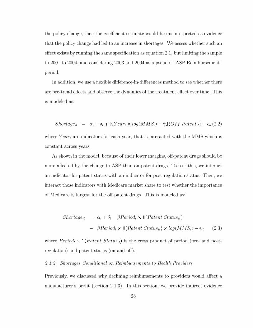
In addition, we use a flexible difference-in-differences method to see whether there
are pre-trend effects and observe the dynamics of the treatment effect over time. This
is modeled as:
Shortageit � αi � δt � βtY eart � logpMMSiq � γ1pOff Patentitq � εit (2.2)
where Y eart are indicators for each year, that is interacted with the MMS which is
constant across years.
As shown in the model, because of their lower margins, off-patent drugs should be
more affected by the change to ASP than on-patent drugs. To test this, we interact
an indicator for patent-status with an indicator for post-regulation status. Then, we
interact those indicators with Medicare market share to test whether the importance
of Medicare is largest for the off-patent drugs. This is modeled as:
Shortageit � αi � δt � βPeriodt � 1pPatent Statusitq
� βPeriodt � 1pPatent Statusitq � logpMMSiq � εit (2.3)
where Periodt � 1pPatent Statusitq is the cross product of period (pre- and post-
regulation) and patent status (on and off).
2.4.2 Shortages Conditional on Reimbursements to Health Providers
Previously, we discussed why declining reimbursements to providers would affect a
manufacturer’s profit (section 2.1.3). In this section, we provide indirect evidence
28

of this effect, by checking whether the reduced reimbursements to providers increase
the rate of shortages. Under the assumption that a majority of the variation in price
was due to the policy change (see Figure 2.3), then most of the variation in price can
be considered exogenous which allows us to use OLS. The specification we use is:
Shortageit � αi � δt � β1logpReimbursement per serviceitq
� β21pPatent Statusitq � εit (2.4)
where Reimbursement per serviceit is the mean reimbursement (revenue divided
by quantity) by Medicare in year t for drug i. In practice, this should be similar
to the AWP or ASP during the respective reimbursement regimes. Drugs which go
into shortage experience increases in price which translate into increased Medicare
reimbursements after 2005 with ASP based reimbursement. Therefore, the OLS
regression will underestimate the effect of drug prices that have risen in response to
shortage. To control for the effect of shortages on prices, we use one-year lagged
reimbursement values.
We also condition on the patent status (1pPatent Statusitq) since it plays impor-
tant roles in the theory. Finally, αi and δt are drug and time fixed effects.
One possible concern in this regression is that unobservable demand shocks are
driving both prices and shortages. However, a positive demand shock would lead to
higher prices and more shortages, holding supply fixed. This biases the estimates
in the opposite direction of what we ultimately find, which is that higher prices are
correlated with fewer shortages.
2.4.3 Shortages Conditional on Manufacturer’s Prices
In the previous section, we analyzed changes in shortage frequency with variation in
reimbursements to health care providers. While the law directly affected reimburse-
29
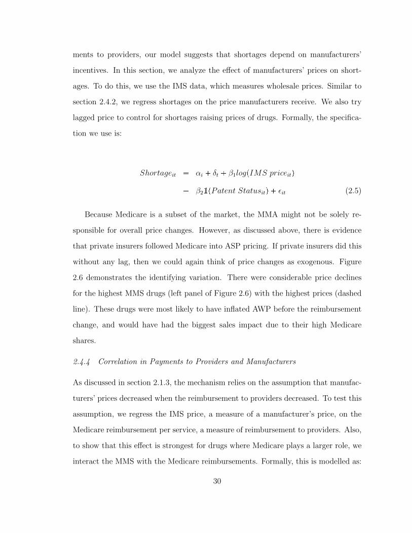
ments to providers, our model suggests that shortages depend on manufacturers’
incentives. In this section, we analyze the effect of manufacturers’ prices on short-
ages. To do this, we use the IMS data, which measures wholesale prices. Similar to
section 2.4.2, we regress shortages on the price manufacturers receive. We also try
lagged price to control for shortages raising prices of drugs. Formally, the specifica-
tion we use is:
Shortageit � αi � δt � β1logpIMS priceitq
� β21pPatent Statusitq � εit (2.5)
Because Medicare is a subset of the market, the MMA might not be solely re-
sponsible for overall price changes. However, as discussed above, there is evidence
that private insurers followed Medicare into ASP pricing. If private insurers did this
without any lag, then we could again think of price changes as exogenous. Figure
2.6 demonstrates the identifying variation. There were considerable price declines
for the highest MMS drugs (left panel of Figure 2.6) with the highest prices (dashed
line). These drugs were most likely to have inflated AWP before the reimbursement
change, and would have had the biggest sales impact due to their high Medicare
shares.
2.4.4 Correlation in Payments to Providers and Manufacturers
As discussed in section 2.1.3, the mechanism relies on the assumption that manufac-
turers’ prices decreased when the reimbursement to providers decreased. To test this
assumption, we regress the IMS price, a measure of a manufacturer’s price, on the
Medicare reimbursement per service, a measure of reimbursement to providers. Also,
to show that this effect is strongest for drugs where Medicare plays a larger role, we
interact the MMS with the Medicare reimbursements. Formally, this is modelled as:
30

Figure 2.6: Prices for Generic Injectable Drugs
On the left are prices for drugs in the top quartile of MMS, meaning used by seniors. The pricesare falling for the drugs with highest prices that are targeted at seniors. On the right are pricesfor the bottom quartile of MMS, meaning used by younger patients. Prices are adjusted to2010 dollars. All percentiles are calculated without weights across drugs. Source: IMS MIDAS
logpIMS Priceitq � β0 � δt � β1logpReimbursement per serviceitq (2.6)
�β2MMSi � logpReimbursement per serviceitq � εi
2.5 Results
The top panel of Table 2.1 gives summary statistics for the main sample. There
are 308 drugs in the main sample. The lower panel gives summary statistics for off
and on-patent drug year observations separately. The average time that a drug is in
shortage was 59 days (unconditional on being in shortage), but was 82 days and 14
days for off- and on-patent drugs, respectively. 66 percent of drug-year observations
are off patent. The average number of manufacturers for an off-patent drug is 3.
31
Using the IMS data, the average MMS is 0.10 and using the MarketScan data the
average MMS is 0.15. The MarketScan MMS measure is larger because it does not
include in the denominator spending by payers like Medicare Advantage, Medicaid,
Veterans Affairs, or spending in settings like inpatient hospitals. In the MarketScan
data, the mean patient age is 45.
There are fewer observations in the Manufacturer Price and Number of Manu-
facturers rows. Manufacturer Price has fewer observations, because our sample of
IMS data is from 2003 to 2010, so earlier and later years are dropped. The row
with the number of manufacturers has fewer observations because some drugs were
not in the Orange Book. Many of the products missing from the Orange Book are
biologics which we assume are on patent (or at least, have no generic competition).
Hence, while many of the observations are missing from the Orange Book, they are
not missing from our analysis.
Figure 2.3 shows the distribution of reimbursement levels (left panel) and changes
(right panel) for off-patent drugs in Medicare. In 2005, there is a large fall in re-
imbursement which is concurrent with the implementation of ASP under the MMA.
Figure ?? in the appendix shows the distribution for all drugs (on and off patent),
which has similar patterns, though less pronounced.
Figure 2.6 shows that IMS prices decline most for generic drugs with high prices
and high MMS. The left panel shows prices for drugs in the bottom quartile of share
of their sales from Medicare, while the right shows the drugs in the top quartile.
We see large, slow price declines in drugs that have a high share of Medicare sales
versus those which do not. This suggests that while not all drugs are affected by the
law change, those most affected were those where the Medicare population plays the
largest role. This is consistent with the idea that Part B is not a huge part of the
market (Medicare is roughly 30 percent of the market, and 30 percent of Medicare is
in Medicare Advantage), but for drugs where it is important, prices fall over time in
32

all markets as other payers switch to ASP. This may help explain the lag in shortages
after the law change.
2.5.1 Results for Shortages Conditional on Medicare Market Share
Table 2.2 presents the difference-in-differences relationship between shortages and
Medicare market share. The estimate is 6.73 in the OLS (Table 2.2, Column 1), and
7.83 in the IV (Table 2.2, Column 2). As expected, the IV estimate is larger due to
the correction of measurement error. The results imply that an increase in the MMS
from the mean of 0.09 to 0.10 leads to a 0.71 and 0.82 day increase in the number
of shortage days, for the OLS and IV estimates, respectively. Columns (1) and (2)
omit age in the instrument set. Using year indicators, we have differenced out the
time-trend in the results. Column (3) is a robustness check where we include age
and age-squared in the instrument set. Columns (4) and (5) use the MarketScan
MMS as the endogenous variable, where column (4) is the OLS estimate and column
(5) is the IV which uses the IMS MMS as an instrument. Using the MarketScan
MMS gives larger point estimates and implied magnitudes. The IV coefficient of
12.88 implies a change from 0.14 to 0.15 in MMS, leads to a 0.89 day increase in
the number of shortages. These estimates show that for a number of specifications,
drugs with higher Medicare market share were more likely to be in shortage after the
MMA went into effect.29
Table 2.3 gives the initial first stage result, where we regress the log of IMS MMS
on the instrument set. Table 2.4 gives the first-stage results in the main regression,
where the interaction of predicted MMS with the ASP reimbursement dummy is
as an instrument for log of IMS MMS interacted with the ASP reimbursement. In
each table, column (1) uses the log of IMS MMS as the endogenous variable and
29 In the first two columns of Table A.2 in the Appendix, we report the results using levels insteadof logs. The results are similar.
33

the log of MarketScan MMS as the instrument, (2) includes age and age-squared
in the instrument set, and (3) uses the log of MarketScan MMS as the endogenous
variable and the log of IMS MMS as the instrument. For the initial first stage, the
F-statistic is well above 10, the usual rule of thumb for instrument relevance in each
specification.
In the main specification we assume the patent expires 15 years after the first
approval. In Table 2.5, we consider alternative specifications. We define off patent as
18 years since first approval in columns (1) and (2), 12 years in columns (3) and (4),
and 8 years in columns (5) and (6).30 Furthermore, unlike our standard definition
of off patent, we do not redefine drugs with multiple manufacturers as off patent as
well. The odd columns are OLS results while the even numbered columns are IV
results. Changing the patent variable leads to differences in the OLS estimate of the
treatment effect from 6.29 to 6.77, and the IV estimate of the treatment effect from
7.11 to 7.88. In summary, we find that varying the patent status variable within
reason matters little for our coefficients of interest.
If drugs with higher Medicare market shares were experiencing an increase in
shortages prior to the policy change, then the coefficient estimate would be misin-
terpreted as evidence that the policy change led to an increase in shortages. Table
2.6 presents a falsification test by choosing a “pseudo”-regulation period and seeing
whether our specification picks up the results. We use 2003 as the regulation year,
rather than 2005, and drop all data starting in 2005. Thus, 2001 and 2002 are the
fake pre-period and 2003 and 2004 are the post-period. The OLS coefficient from
the MMS interacted with a post regulation indicator falls from 6.73 to -0.61 in this
falsification test and loses statistical significance. Likewise, the IV coefficient falls
from 7.83 to 1.39 and loses statistical significance as well. These results suggest in
30 We use 8 years as the minimum because drugs submitting clinical evidence receive 5 years ofdata exclusivity plus an additional 2.5-year stay for the courts to sort out a patent challenge.
34

the pre-period, the assumption of parallel trends holds, a check that is often used in
the literature to justify the parallel trends-assumption during the sample period.
To better understand how the effects of MMS change over time, Table 2.7 presents
the OLS and IV estimates of our specification using yearly treatment indicators
interacted with the MMS. The OLS coefficient for 2007 is 6.63, which suggests a 0.70
day difference in shortages for drugs with 0.09 MMS versus those with 0.1 MMS,
compared to the omitted year of 2001. The coefficients prior to 2005 are insignificant.
In 2004 the magnitudes of both the OLS and the IV start growing and the coefficient
estimates start becoming statistically different than zero. This corresponds to the
switch from 95 percent AWP to 85 percent AWP in 2004 to ASP �6 percent in 2005.
Afterwards, the coefficients stabilize at higher levels, roughly 7 for the OLS and 10
for the IVs until the end of the sample. This highlights that the results are not due
to just one year, as well as some lag time for the MMA to matter for drug shortages.
Finally, our theoretical model suggests that the reimbursement change should
impact off-patent drugs more than on-patent drugs, because off-patent drugs have
small margins. Hence, we interact the off-patent indicator with a post-regulation
indicator and the MMS measure (Table 2.8). Because the off-patent indicator is
interacted with several other variables, we sum the coefficients. The coefficients
on the off-patent interaction terms sum to as little as 86 (Table 2.8, Column 4)
and as much as 95 (column 5). Hence, off-patent drugs are associated with about
3 additional months of shortages. Furthermore, the effect of off-patent status on
shortages is greatest after 2005 as indicated by the positive coefficients on the inter-
action between off patent and the post period. These results corroborate our theory
that off-patent drugs, which tend to have lower reimbursement, should be most in
shortages and most affected by the reimbursement change.
35
2.5.2 Results for Shortages Conditional on Reimbursements to Health Providers
Table 2.9 shows the results for shortages conditional on reimbursements to providers.
Columns (1) and (2) show the log and lagged-log reimbursement coefficients. The
coefficient on lagged reimbursement suggests that a 1 percent (roughly 81 cents per
unit) decrease in reimbursement leads to 0.30 more shortage days. Columns (3) and
(4) show the same results keeping only drugs which were off patent throughout the
sample while columns (5) and (6) show the on-patent results. Consistent with our
theory, off-patent drugs were most affected by prices. The statistically significant
coefficient on a one-year lag of log price for an off-patent drug of -40.27 suggests that
a 1 percent decrease in price (roughly 32 cents per unit) leads to 0.40 more shortage
days. The on-patent drugs’ results were negative and not statistically significantly
different from zero, which is consistent with our theory that these drugs had higher
margins. The change in estimates moving from current price to the 1 year lagged
price (-26.88 to -30.29) are consistent with correcting the downward bias caused by
the reverse causality problem described above.
2.5.3 Results for Shortages Conditional on Manufacturers’ Prices
Table 2.10 shows the results for shortages conditional on manufacturers’ prices.
Columns (1) and (2) show the log and lagged-log price coefficients. The coefficient
on lagged price suggests that a 1 percent (roughly 2.87 dollars per unit) decrease in
price leads to 0.36 more shortage days. Columns (3) and (4) show the same results
keeping only drugs which were off patent throughout the sample while columns (5)
and (6) show the on-patent results. Again, off-patent drugs were most affected by
prices. The statistically significant coefficient on 1 year lag of log price of -29.91 sug-
gests that a 1 percent decrease in price (roughly 93 cents per unit) leads to 0.30 more
shortage days. The on-patent drugs’ results, as in the case with reimbursements to
health providers, were not statistically significant. In summary it appears that lower
36

prices to manufacturers are correlated with more shortages.
2.5.4 Results for Correlation in Payments to Providers and Manufacturers
Table 2.11 reports the correlation in payments. On average, a ten percent decline
in Medicare reimbursement would reduce the manufacturer’s price by 3.4 percent.
Drugs which have higher Medicare market share should be more affected by Medicare
price changes. To account for this, we interact the share of revenue coming from
Medicare. The interaction term, while statistically insignificant, is important in
magnitude. Added to β1, the coefficient implies that a 10 percent decline in Medicare
reimbursement could reduce the price a manufacturer gets by close to 4.6 percent
near the maximum on MMS. This is suggestive of the magnitude of pass through in
reimbursement reductions from the law to manufacturers.
2.6 Discussion
We analyzed the effect of a reimbursement change on drug shortages using several ap-
proaches. Our main approach was a difference-in-differences (pre/post and Medicare
market share) with drug and year fixed effects. We found that the reimbursement
change led to about 2 additional weeks (13 days) of shortages for generic injectables
(Column 5 of Table 2.2). We also used a triple difference without fixed effects and
again found that shortages of generic injectables increased by about 2 weeks (13
days) (Column 5 of Table 2.8). Finally, we used reimbursement on the right side of
the regression equation to examine directly how reimbursement affected shortages.
We found that a 50 percent drop in reimbursement (Office of Inspector General,
2005) led to about 2 additional weeks (16 days) of shortages for generic injectables
(Table 2.9).
We provide evidence that higher reimbursement could reduce drug shortages. A
10 percent increase in Medicare reimbursement for an off patent drug is associated
37

with 4 fewer days of shortage (Table 2.9). A 10 percent increase in price for all off-
patent drugs is about $3.24 per service (Table 2.1). With roughly 50 million services
per year (699 million services across 12 years), and at $3.24 per service, that equals
$162 million dollars to avert 4 days of shortages for the average injectable or infused
drug. Alternatively, the payment increases could target lower-priced drugs, as would
be sensible according to our model.31 A payment increase of 10 percent for off-patent
drugs under the 90th percentile of reimbursement levels would amount to $0.71 per
service. For off-patent drugs below the 50th percentile, the increase would be $0.12
per service. Focusing on these least cost drugs, for example by targeting drugs in
the lower half of the reimbursement level distribution, would allow for a reduction in
total shortages of nearly 2 weeks (12.5 days) at a cost of about $50 million dollars.32
Other factors may be associated with drug shortages. First, declining drug prices
resulted not only from Medicare changes, but also from the expansion of 340B pric-
ing (as discussed in section 2.1.2). However, the scale of the 340B program is much
smaller than the scale of Medicare, with the 340B program accounting for only
about 2 percent of U.S. drug sales (U.S. Department of Health and Human Services,
2013, 311). Second, industry consolidation could cause shortages. However, con-
solidation among manufacturers has ambiguous effects. Consolidation could make
shortages less likely as consolidation increases market power and margins. Alter-
natively, depending on the covariance of shocks to manufacturing lines of different
firms, consolidation could lead to increased shortages. Third, shortages could be
caused by grey-market distributors and stockpiling by hospitals, but these practices
are symptoms of shortages, rather than causes. Finally, increased FDA regulatory
31 In columns (3) and (4) in Table A.2 in the Appendix, we show that the main regression resultshold within the sample of lower-price generic drugs as defined by prices below the median.
32 The total cost to society depends on how private payment reacts as well. If private paymentfollows Medicare reimbursement, then it would be more expensive. In fact, not all private insurerschanged and even those that changed did not move all the way down to ASP plus 6 percent, so thecost would be less than $750 million.
38
scrutiny appears to be associated with drug shortages (Stomberg, 2015). However,
some of the increased scrutiny could be a reaction to less investment in reliabil-
ity by the manufacturers. The aforementioned factors are complementary but not
competing hypotheses. For FDA regulatory scrutiny to be a competing hypothesis,
increased FDA scrutiny would have to take place after the policy change and fall
disproportionately on generic drugs which served more Medicare patients.
The policy change was implemented in 2005, but shortages did not become large
until 2009. However, the empirical analysis shows an increase in shortages for drugs
with higher MMS starting in 2006. Furthermore, private insurers are known to
mimic Medicare with a lag (as described in section 2.1.2). Finally, some manufactur-
ers probably continued to produce these low-margin drugs until other opportunities
arose, such as following a large wave of patent expirations in 2007.
The generic sterile injectable market shares several features with electricity gener-
ation. First, timing is critical. In the generic market, delays can be costly to patient
health, and in electricity, supply and demand must be in equilibrium at each instant
to avoid power system failures. Second, storage is costly. Sterile injectables are
sensitive to light and temperature. Likewise, storing electricity by battery or with
hydro storage is currently considered prohibitively costly in most cases. Third, there
is little product differentiation, so price competition can be fierce. The solution in
electricity generation has been a mixture of rapid price adjustment and government
regulation (Cramton and Stoft, 2005).
Another approach to reducing shortages would be to write contracts with “failure
to supply” clauses. If contracts impose harsh penalties on manufacturers for failure
to supply, then shortages should fall and average prices should rise. However, con-
tracts might be difficult to enforce due to information asymmetries. Furthermore,
contracts usually void the penalty in the case of nationwide shortages (U.S. Depart-
ment of Health and Human Services, 2011). Another concern is that contracts might
39

encourage the buyer to create a shortage by hoarding, thus receiving a penalty pay-
ment from the supplier. Alternatively, competing suppliers might hoard to create
a shortage and then supply the product when prices rise. Given that the shortage
problem is relatively recent, perhaps buyers will learn to write new contracts that
reduce the shortage problem.
Finally, there might be a role for regulation. For example, the Food and Drug
Administration Safety and Innovation Act (FDASIA) of 2012 requires that manu-
facturers notify FDA of potential discontinuances.
2.7 Conclusion
Shortages of drugs, especially generic sterile injectable drugs, increased dramatically
beginning in the mid-2000s. The increase in shortages followed a change in drug
reimbursement. We show that a reduction in reimbursement to health providers
was passed to manufacturers and played a role in the large increase in shortages
of generic sterile injectable drugs. Drugs used to treat diseases with high Medicare
share were most affected by the reimbursement change. The results are consistent
with a model in which declining reimbursement decreased the returns to investing in
manufacturing capacity and reliability which led to an increase in drug shortages.
To reduce shortages, Medicare could increase reimbursement. Both the theoreti-
cal model and the empirical results suggest that firms with market power (and thus
higher prices) tend to invest more in capacity and have fewer shortages. Of course,
increasing prices through higher reimbursement and/or market power is costly. The
optimal number of shortages is not necessarily zero if it requires extremely high
prices. However, reimbursement increases could focus on lower-priced drugs. We
show that for the cheapest generic drugs, a payment increase of $0.12 per service
would cost about $50 million and reduce shortages by about 2 weeks.
40

Table 2.1: Descriptive Statistics
source count mean sd min maxShortage Days Univ. Utah 3094 59.28 120.23 0.00 365.00Number of Manufacturers Orange Book 2679 3.04 2.94 0.00 25.00MMS IMS 3094 0.10 0.17 0.00 1.00MMS MarketScan 3094 0.15 0.17 0.00 0.93Medicare Reimbursement ($) Part B 3094 81.03 261.96 0.00 3645.59Mean Age (years) MarketScan 3094 45.34 7.42 12.83 57.92Off Patent Orange Book 3094 0.66 0.47 0.00 1.00Manufacturer Price ($) IMS 2030 286.90 672.92 0.01 12533.00Observations 3094
Off Patent On Patentsource count mean sd count mean sd
Shortage Days Univ. Utah 2050 82.40 135.77 1044 13.87 59.48Number of Manufacturers Orange Book 2050 3.68 3.09 629 0.95 0.22MMS IMS 2050 0.09 0.16 1044 0.14 0.19MMS MarketScan 2050 0.13 0.15 1044 0.19 0.20Medicare Reimbursement ($) Part B 2050 32.40 118.54 1044 176.52 402.64Mean Age (years) MarketScan 2050 44.42 6.83 1044 47.14 8.17Off Patent Orange Book 2050 1.00 0.00 1044 0.00 0.00Manufacturer Price ($) IMS 1315 93.47 383.64 715 642.66 905.71Observations 2050 1044
Descriptive statistics for the 308 drugs in the sample from 2001 to 2012. MMS is Medicare Market Share.
41

Table 2.2: OLS and IV Estimates of the Effect of MMS on Shortage Days
(1) (2) (3) (4) (5)Off Patent -5.200 -5.449 -5.454 -6.763 -7.576
(13.54) (13.51) (13.52) (13.57) (13.46)
Year ¥ 2005 � Log MMS 6.732*** 7.828*** 7.852*** 10.20*** 12.88***(2.192) (2.925) (2.932) (3.648) (4.021)
Constant 17.70* 18.62**(9.286) (9.287)
Observations 3094 3094 3094 3094 3094# Drugs 308 308 308 308 308R2 0.172 0.172 0.172 0.172 0.171Drug Fixed Effect Yes Yes Yes Yes YesYear Fixed Effect Yes Yes Yes Yes YesIV Regression No Yes Yes No Yes* p 0.10, ** p 0.05, ***p 0.01
Standard errors, in parentheses, are clustered at the drug level. The dependent variable isshortage days in a year. Off patent is 15 years since earliest Orange Book approval. Columns(1) and (2) are the OLS and IV estimates using the IMS MMS as the treatment variable,respectively. Column (3) includes age in the instrument set. Column (4) and (5) are theOLS and IV estimates using the MarketScan MMS as the treatment variable. Each regressioncontains molecule fixed effects and indicator variables for each year from 2002 to 2012.
42

Table 2.3: First Stage - MarketScan MMS on IMS MMS
(1) (2) (3)Log MMS 1.223*** 1.215*** 0.561***
(0.0473) (0.0518) (0.0217)
Mean Age -0.198**(0.0896)
Mean Age Squared 0.00244**(0.00108)
Constant -0.855*** 2.946 -0.468***(0.175) (1.873) (0.120)
Observations 308 308 308R2 0.686 0.691 0.686F-stat 668.0 226.6 668.0* p 0.10, ** p 0.05, ***p 0.01
Standard errors, in parentheses, are clustered at the drug level. First step in IVs, OLS with logof MarketScan MMS as the independent variable and log of IMS MMS as the dependent variable.Column (1) is the single instrument case. Column (2) adds age instruments. Column (3) useslog of MarketScan MMS as the dependent variable and log of IMS MMS as the independentvariable.
Table 2.4: First Stage - Predicted MMS � Year ¥ 2005
(1) (2) (3)Off Patent -0.168 -0.180 0.184**
(0.167) (0.160) (0.0791)
Predicted Log MMS 1.065*** 1.063*** 0.932***(0.0504) (0.0507) (0.0578)
Observations 3094 3094 3094# Drugs 308 308 308R2 0.905 0.907 0.911F-stat 177.0 176.0 166.4* p 0.10, ** p 0.05, ***p 0.01
Standard errors, in parentheses, are clustered at the drug level. This is the first-stage in 2SLSwhere the instrument is predicted MMS from Table 2.3 interacted with ASP Reimbursement.The first column in the main specification. The second is using age as an additional instrument.The third uses the MarketScan MMS instead of the IMS MMS. Each regression also containsindicator variables for each year from 2002 to 2012, which are omitted from the table.
43

Table 2.5: Robustness Check: Different Patent Definitions
(1) (2) (3) (4) (5) (6)Off Patent 69.84*** 69.55***-10.51 -10.78 -19.92* -19.83*
(18.44) (18.35) (12.82) (12.80) (11.10) (11.15)
Year ¥ 2005 � Log MMS 6.290*** 7.108** 6.765*** 7.877*** 6.671*** 7.703***(2.147) (2.849) (2.197) (2.938) (2.202) (2.948)
Constant -16.97* 20.48** 27.68***(9.862) (8.274) (8.715)
Observations 3094 3094 3094 3094 3094 3094# Drugs 308 308 308 308 308 308R2 0.184 0.184 0.172 0.172 0.173 0.173Drug Fixed Effect Yes Yes Yes Yes Yes YesYear Fixed Effect Yes Yes Yes Yes Yes YesIV Regression No Yes No Yes No Yes* p 0.10, ** p 0.05, ***p 0.01
Standard errors, in parentheses, are clustered at the drug level. The dependent variable isshortage days in a year. Odd-numbered columns are OLS and even-numbered columns are IV.We define off patent as years since earliest Orange Book approval. In the main specification,off patent means 15 years since approval. In Columns (1) and (2), off patent means 18 yearssince approval. In Columns (3) and (4), off patent means 12 years since approval. In Columns(5) and (6), off patent means 8 years since approval.
44

Table 2.6: Falsification Test Using 2003 as Regulation Year
(1) (2)Off Patent 29.83 27.47
(26.14) (26.52)
Year ¥ 2003 � Log MMS -0.608 1.390(2.440) (2.697)
Constant 3.340(18.54)
Observations 896 879# Drugs 246 229R2 0.0633 0.0617Drug Fixed Effect Yes YesYear Fixed Effect Yes YesIV Regression No Yes* p 0.10, ** p 0.05, ***p 0.01
Standard errors, in parentheses, are clustered at the drug level. The dependent variable isshortage days in a year. This regression uses 2003, rather than 2005, as a false policy year.2003 and 2004 are considered treatment years, data from 2005 and onwards are dropped. Offpatent is 15 years since earliest Orange Book approval. Columns (1) and (2) are the OLSand IV estimates using the IMS MMS as the treatment variable, respectively. Each regressioncontains molecule fixed effects and indicator variables for each year from 2002 to 2004.
45

Table 2.7: OLS and IV Year By Year Coefficient Estimates
(1) (2)Off Patent -5.635 -7.220
(13.64) (13.72)
Year=2002 � Log MMS -2.036 -1.142(2.058) (2.502)
Year=2003 � Log MMS -1.789 -0.452(3.130) (3.705)
Year=2004 � Log MMS 0.597 5.381(2.915) (3.343)
Year=2005 � Log MMS 5.006* 8.252**(2.981) (3.775)
Year=2006 � Log MMS 4.845* 7.353*(2.892) (3.913)
Year=2007 � Log MMS 6.633** 10.09**(2.778) (4.025)
Year=2008 � Log MMS 7.967*** 12.07***(2.993) (3.844)
Year=2009 � Log MMS 7.856** 13.39***(3.384) (3.888)
Year=2010 � Log MMS 5.886* 10.04***(3.350) (3.632)
Year=2011 � Log MMS 6.457 8.620*(3.940) (4.650)
Year=2012 � Log MMS 2.908 3.181(3.976) (4.755)
Constant 17.89*(9.478)
Observations 3094 3094# Drugs 308 308R2 0.174 0.172F-stat 10.88 11.10Drug Fixed Effect Yes YesYear Fixed Effect Yes YesIV Regression No Yes* p 0.10, ** p 0.05, ***p 0.01
Standard errors, in parentheses, are clustered at the drug level. The dependent variable isshortage days in a year. Columns (1) and (2) are the OLS and IV estimates, respectively. Eachregression contains molecule fixed effects and indicator variables for each year from 2002 to2012.
46

Table 2.8: The Effect of the Reimbursement Change and Patent Status on Shortage Days
(1) (2) (3) (4) (5)Off Patent 22.46 23.63 24.17 29.11* 16.27
(16.40) (20.51) (20.57) (17.49) (19.37)
Log MMS -2.073 -3.087 -3.229 -4.477 -3.865(1.873) (2.064) (2.077) (3.053) (3.520)
Log MMS � Off Patent -4.785 -4.452 -4.321 -4.525 -8.832(3.440) (4.477) (4.493) (5.542) (6.355)
Year ¥ 2005 -1.218 2.079 0.746 1.349 0.195(9.679) (10.32) (10.38) (9.840) (10.82)
Year ¥ 2005 � Off Patent 65.31*** 61.26*** 62.65*** 54.69*** 74.20***(17.97) (22.96) (23.03) (19.72) (21.22)
Year ¥ 2005 � Log MMS 1.865 2.649 2.317 3.932 3.493(1.901) (1.938) (1.974) (2.862) (3.542)
Year ¥ 2005 � Log MMS � Off Patent 6.907* 5.952 6.297 6.417 12.98*(3.693) (4.738) (4.767) (5.859) (6.836)
Constant 11.77 7.538 6.945 8.580 10.20(9.246) (9.921) (9.965) (9.488) (10.34)
Observations 3094 3094 3094 3094 3094# Drugs 308 308 308 308 308R2 0.0849 0.0846 0.0845 0.0834 0.0822Drug Fixed Effect No No No No NoYear Fixed Effect No No No No NoIV Regression No Yes Yes No Yes* p 0.10, ** p 0.05, ***p 0.01
Standard errors, in parentheses, are clustered at the drug level. The dependent variable isshortage days in a year. Off patent is 15 years since earliest Orange Book approval. Columns(1) and (2) are the OLS and IV estimates using the IMS MMS as the treatment variable,respectively. Column (3) includes age in the instrument set. Column (4) and (5) are the OLSand IV estimates using the MarketScan MMS as the treatment variable. This table does notcontain molecule fixed effects and indicator variables for each year.
47
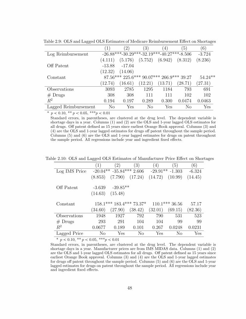
Table 2.9: OLS and Lagged OLS Estimates of Medicare Reimbursement Effect on Shortages
(1) (2) (3) (4) (5) (6)Log Reimbursement -26.88***-30.29***-32.19***-40.27***-8.506 -3.724
(4.111) (5.176) (5.752) (6.942) (8.312) (8.236)Off Patent -13.88 -17.04
(12.32) (14.06)Constant 87.56*** 225.6*** 90.07*** 266.9*** 39.27 54.24**
(12.74) (16.61) (12.21) (13.71) (28.71) (27.31)Observations 3093 2785 1295 1184 793 691# Drugs 308 308 111 111 102 102R2 0.194 0.197 0.289 0.300 0.0474 0.0463Lagged Reimbursement No Yes No Yes No Yes* p 0.10, ** p 0.05, ***p 0.01
Standard errors, in parentheses, are clustered at the drug level. The dependent variable isshortage days in a year. Columns (1) and (2) are the OLS and 1-year lagged OLS estimates forall drugs. Off patent defined as 15 years since earliest Orange Book approval. Columns (3) and(4) are the OLS and 1-year lagged estimates for drugs off patent throughout the sample period.Columns (5) and (6) are the OLS and 1-year lagged estimates for drugs on patent throughoutthe sample period. All regressions include year and ingredient fixed effects.
Table 2.10: OLS and Lagged OLS Estimates of Manufacturer Price Effect on Shortages
(1) (2) (3) (4) (5) (6)Log IMS Price -20.04** -35.84*** 2.606 -29.91** -1.303 -6.324
(8.853) (7.790) (17.24) (14.72) (10.99) (14.45)
Off Patent -3.639 -39.85**(14.63) (15.48)
Constant 158.1*** 183.4*** 73.37* 110.1*** 36.56 57.17(34.60) (27.90) (38.42) (32.01) (69.15) (82.36)
Observations 1948 1927 792 790 531 523# Drugs 293 291 104 104 99 99R2 0.0677 0.189 0.101 0.267 0.0248 0.0231Lagged Price No Yes No Yes No Yes* p 0.10, ** p 0.05, ***p 0.01
Standard errors, in parentheses, are clustered at the drug level. The dependent variable isshortage days in a year. Manufacturer prices are from IMS MIDAS data. Columns (1) and (2)are the OLS and 1-year lagged OLS estimates for all drugs. Off patent defined as 15 years sinceearliest Orange Book approval. Columns (3) and (4) are the OLS and 1-year lagged estimatesfor drugs off patent throughout the sample period. Columns (5) and (6) are the OLS and 1-yearlagged estimates for drugs on patent throughout the sample period. All regressions include yearand ingredient fixed effects.
48

Table 2.11: Effect of Medicare Reimbursement on Price to Manufacturers
(1) (2) (3) (4) (5) (6)Log Medicare Reimbursement 0.352*** 0.339*** 0.237*** 0.206*** 0.0582 0.0619
(0.0524) (0.0593) (0.0508) (0.0550) (0.0371) (0.0395)
Log Medicare Reimbursement � MMS 0.129 0.195 -0.125(0.187) (0.182) (0.178)
Constant 2.827*** 2.809*** 1.834*** 1.828*** 5.461*** 5.518***(0.129) (0.124) (0.0824) (0.0797) (0.131) (0.142)
Observations 2029 2029 848 848 533 533# Drugs 304 304 111 111 100 100R2 0.284 0.285 0.164 0.172 0.0600 0.0615* p 0.10, ** p 0.05, ***p 0.01
Standard errors, in parentheses, are clustered at the drug level. This table regresses Medicare prices on IMS prices. Columns (1), (3) and(5) regress log Medicare price on IMS price, with year and drug fixed effects. Columns (2), (4) and (6) add an interaction between Medicaremarket share with the Medicare price. Columns (1) and (2) include all drugs. Columns (3) and (4) include drugs which are off patentthroughout the sample. Columns (5) and (6) include drugs which are on patent throughout the sample.
49

3
Bargaining in Markets with Exclusion:An Analysis of Health Insurance Networks
Spending on health care in the United States totals three trillion dollars per year,
more than 350 billion dollars of which is spent by private insurance companies at
hospitals.1 Because of this high spending, policy makers and insurance companies
have a considerable interest in controlling health care costs. One aspect of cost
control used by insurance companies is to form networks. An insurance network
is a list of providers which the insurance company incentivizes its patients to visit.
Patients who visit a provider outside of their insurance network often face reduced
or no coverage for those services.2
This paper formalizes and explores the implications of a common story among
health care insiders: that the threat of exclusion from networks improves insurers’
bargaining leverage in their negotiations with providers. Howard (2014) provides
one example of this intuition: “Networks give insurers leverage in their negotiations
1 Source: National Health Expenditure Accounts, The Centers for Medicare and Medicaid Services.
2 For example, out of network visits may have a higher copay, higher coinsurance or the paymentsdo not factor into the deductible.
50
with providers over reimbursement rates. Insurers rely on the threat of exclusion
rather than the actual narrowness of their networks – providers that do not face the
threat of exclusion have little reason to temper their demands for higher prices.” In
my data, plans that exclude providers, often referred to as “narrow networks,” pay
23 percent less at the same hospital for the same services. I present this result as
suggestive evidence that the bargaining leverage theory may account for substantial
savings, while other mechanisms that explain why narrow networks reduce insurers’
costs cannot easily explain this comparative static.3
Despite their cost savings, narrow-network health insurance plans are controver-
sial.4 The concern among regulators is that patients lack information about which
conditions they will get in the future; without knowing what conditions they will
have in the coming year, they may not check whether high quality providers are
available in each specialty. This concern has grown due to the prevalence and pop-
ularity of narrow-network health plans in the insurance marketplace (referred to as
“exchanges”) set up by the Affordable Care Act (ACA). In a national study, Bauman
et al. (2014) find that 45 percent of plans on the ACA health insurance exchanges
have narrow networks, and in my sample 71 percent of patients are enrolled in a
plan with a narrow network.5 These plans are popular because, while they provide
fewer options for care, they also charge lower premiums to consumers. For example,
Bauman et al. (2014) find that narrow-network plans charge premiums 13-17 percent
lower than broad-network plans.6
3 I discuss other mechanisms in section 3.1.4.
4 See Howard (2014), Corlette et al. (2014), or Baicker and Levy (2015) for more details on thepolicy discussion about restricting narrow networks.
5 Bauman et al. (2014) define a narrow-network health plan as having less than 70 percent of thatmarket’s hospitals in network. I follow their definition for this analysis. They find that roughly90 percent of patients have access to narrow-network plans, but 90 percent also have access tobroad-network health plans.
6 Their results control for metal level (a measure of the actuarial value of the plan), insurancecompany, plan type (e.g., HMO or PPO) and location.
51
There is considerable policy interest around regulating these plans. The ACA
included the first federal “network adequacy” law, which sets standards that networks
must meet, though it left defining “adequate” to the states. Many states have since
updated or are considering updating their regulations (Giovannelli et al., 2015).7
However, careful regulation requires a trade off between the value of extra access
to providers and higher premiums due to reduced insurer bargaining leverage. One
of the main contributions of this paper is to provide an empirical framework to better
understand why, and how much, restricting insurers’ ability to exclude would raise
costs. I argue that a structural model is needed to evaluate how much these laws
would raise costs, since a reduced-form analysis may suffer from a bias due to the
endogeneity of these networks.
To formalize how an insurer can use the threat of exclusion to gain leverage, I
propose a novel model of price formation in a bilateral oligopoly setting where the
networks are endogenous. My model nests the Nash-in-Nash bargaining model, which
has become the workhorse model of vertical competition; when exclusion is assumed
to be exogenous my model is identical to Ho and Lee (2017).8 Therefore, my model
shares many of the advantages of the Nash-in-Nash model, it is in a bilateral oligopoly
setting, allows for heterogeneity in the amount of available surplus and accounts
for externalities and interdependencies between hospitals and insurers. However,
allowing for the endogeneity of the networks allows me to capture two important
institutional features of this market: the insurer uses the threat of exclusion to gain
bargaining leverage, and exclusion is an equilibrium outcome of this model.
7 Another common restriction on exclusion is an “any willing provider” law, which requiresinsurance companies to cover all medical providers willing to agree to the terms offered bythe plan. In 2014, 27 states had passed some form of any willing provider law, though inmany states this does not apply to hospitals. Source: http://www.ncsl.org/research/health/
any-willing-or-authorized-providers.aspx
8 Other papers which use the Nash-in-Nash bargaining model include: Crawford and Yurukoglu(2012a), Grennan (2013b), Gowrisankaran et al. (2014), Beckert et al. (2015), Crawford et al.(2016), Soares (2016) and Prager (2016) among others.
52
The model also allows for richer forms of competition between hospitals than the
Nash-in-Nash model. In the spirit of Town and Vistnes (2001), my model allows
excluded hospitals, which may be substitutes for those in the observed network, to
effect the negotiations of hospitals who will reach an agreement. For example, an
insurer’s threat to exclude a particular hospital may be more salient if there is a
similar hospital to replace it with. A drawback of the Nash-in-Nash model is that
negotiations are not affect by excluded hospitals.
To estimate this model, I use data from the Colorado All-Payer Claims Database
(APCD), which is one of the few sources used in this literature that provides in-
formation on negotiated prices between all insurers and all hospitals.9 The setting
for my study is the non-group market in the Denver, Colorado rating area.10 The
non-group market is where individuals purchase insurance when it is not available
through their employer and they are not eligible for government insurance (e.g.,
Medicare, Medicaid, Tricare, etc.). The ACA exchanges are included in the non-
group market. As such, this is among the first papers which studies competition on
the ACA exchanges.11
Games with randomly ordered sequential agreements, which are commonly used
in the literature where prices and networks are endogenous, can be difficult to es-
timate, especially when externalities between players are allowed.12 However, the
9 Panhans (2016) also uses the Colorado APCD. The other dataset which has been used in this liter-ature and has negotiated prices between all insurers and hospitals in a market is the MassachusettsAPCD. The Massachusetts APCD is used by Ericson and Starc (2015), Shepard (2016), Prager(2016), and Ghili (2016). The Denver, Colorado insurance market has many different features thanthe Massachusetts market. For example, in 2014, Colorado had 10 insurers on its exchange andan additional two off its exchange, but in the non-group market. Ericson and Starc (2015) andShepard (2016)’s sample has five insurer’s.
10 A rating area is a state-defined collection of counties where an insurance company in the non-group market may not vary premiums, except by age and whether the person purchasing insuranceis a tobacco user.
11 Other papers which examine competition on the ACA exchanges include Kowalski (2014), Dafnyet al. (2015), Tebaldi (2016), and Panhans (2016).
12 Abreu and Manea (2012), Manea (2015) and Elliott and Nava (2015) are examples of papers in
53

main insight of the estimation section, and one reason for extending the Nash-in-
Nash model, is that the networks form simultaneously, which simplifies estimation
considerably. Extending the Nash-in-Nash model also allows me to compare my es-
timates with the hospital-insurer bargaining literature. This literature uses a rich
model of the health insurance market to understand how consumer preferences over
premiums, networks, and hospitals affect price formation. The bargaining model is
only one stage of that broader model. I use the same model of consumer preferences
over hospitals and health plans as Ho and Lee (2017) and Prager (2016) to isolate the
contribution of the new bargaining stage from other features of this broader model.
While the role of exclusion is important for policies affecting how insurers form
their networks, the Nash-in-Nash bargaining parameters are also policy relevant. If
hospitals have a lot of relative bargaining power, then restricting one of the insurer’s
tools to gain leverage may have a large effect on prices. On the other hand, if insurers
have a lot of relative bargaining power, even without the use of exclusion, then these
policies would not impact prices much.
To show that ignoring exclusion in estimation can be problematic, I analyze
the effects of a counterfactual law where insurers are not allowed to exclude (i.e.,
a network adequacy law). The Nash-in-Nash model suggests that under the law
prices would fall by 36 percent; plans that had narrow networks prior to the law now
would distribute their enrollees across more hospitals, reducing the marginal surplus
provided by any given hospital. However, by removing the bargaining leverage that
exclusion provides, my model suggests that the law would increase the prices insurers
pay by 50 percent, which is consistent with conventional wisdom that restricting
narrow networks would increase costs for insurers.
The remainder of this paper is organized as follows. Section 3.1 discusses the
related literature and other theories about why narrow-network plans lower costs
this literature.
54

for insurers. Sections 3.2 and 3.3 discuss the data I use and reduced-form evidence.
Section 3.4 presents a stylized model to demonstrate how exclusion can lead to lower
prices for the insurer and why it is an optimal strategy for the insurer. Section 3.5
discusses the computation of surplus and then, given the surplus values, estimation
of the bargaining model. Sections 3.6 and 3.7 discuss the results and counterfactual
estimates. Section 3.8 discusses limitations, extensions, and next steps. Section 3.9
concludes.
3.1 Literature Review
I highlight the contribution of my paper in three literatures: (1) a reduced-form
literature on the savings from managed care, (2) theory on exclusion and bargaining
over networks, and (3) the Nash-in-Nash bargaining model. The final subsection
discusses other proposed mechanisms for why narrow-network plans may save money
for insurers.
3.1.1 Reduced-Form Estimates of Savings from Managed Care
Narrow networks are one strategy that “managed care” plans, such as health main-
tenance organizations (HMOs), use to reduce costs. Other strategies include in-
centivizing physicians to limit utilization, requiring a primary care gatekeeper to
approve specialist visits, and more aggressive cost sharing.13 Much of the literature
quantifying the savings from managed care do not separately account for the role
of networks, which is a limitation of my paper as well.14 Most of the papers in the
literature find large savings comparing managed care prices relative to fee-for-service.
Gruber and Mcknight (2016), Cutler et al. (2000), and Altman et al. (2003) all look
at per patient costs or cost per episode of care, and find savings around 30-40 per-
13 Cost sharing refers to using copay or coinsurance to limit patients’ use of services.
14 As discussed in Cutler et al. (2000), these other strategies are primarily used to reduce utilization.However, Prager (2016) highlights how cost sharing may spillover into bargaining.
55

cent, controlling for patient mix. However, cost per patient may include differences
in utilization intensity.15 Wu (2009) and Dor et al. (2004) examine negotiated prices
per procedure, which should not be affected by patient mix or utilization intensity,
and is consistent with the unit being negotiated over. Wu (2009) and Dor et al.
(2004) find effects of 26-50 percent and 20 percent, respectively. The estimates in
my reduced-form analysis also use price per procedure and the magnitude of my find-
ings are consistent with this literature. I also attempt to distinguish between lower
negotiated prices and narrow-network plans shifting patients to cheaper hospitals.
3.1.2 Theory on Exclusion and Bargaining Over Networks
This paper is related to a broad theoretical literature on competition in vertical
relationships and exclusive dealing.16 It is most closely related to Gal-Or (1997),
who demonstrates in a stylized two-by-two model of hospital-insurer bargaining that
exclusion can lead to insurers negotiating lower prices and can be an equilibrium out-
come. Lee and Fong (2013) propose a dynamic model of hospital-insurer bargaining,
where the networks are determined by a cost of agreement and dynamic consider-
ations. This paper also contributes to the sparse empirical literature on exclusive
dealing.17
This paper is also related to a recent literature on bargaining when prices and
networks are endogenous. This includes Abreu and Manea (2012), Manea (2015)
and Elliott and Nava (2015). Within this literature, my paper is closest to Camera
and Selcuk (2010) who show how an endogenous capacity constraint can be used to
negotiate lower prices. The models in this literature are all very stylized; my model
15 Patient mix refers to how sick patients are. Utilization refers to how many services a patientreceives, conditional on how sick they are.
16 See Rey and Tirole (2007) or Whinston (2008).
17 These include Sass (2005), Lee (2013), Asker (2016) and Soares (2016). See Lafontaine andSlade (2008) for a summary.
56

differs in that it allows for more heterogeneity and I use simultaneous agreement in
order to simplify estimation.
3.1.3 Nash-in-Nash Bargaining Model
The literature on bargaining has a long history starting with the axiomatic approach
to bargaining proposed by Nash (1950). Crawford and Yurukoglu (2012a) extends the
Nash bargaining solution to a bilateral oligopoly setting by invoking the bargaining
protocol of Horn and Wolinsky (1988); each negotiation is modeled as a pairwise
Nash bargaining solution, conditional on the outcome of all other negotiations. That
is, it is a Nash equilibrium of Nash bargains, hence “Nash-in-Nash”. Collard-Wexler
et al. (2016) provides non-cooperative foundations of the Nash-in-Nash model with an
alternating offers, many-to-many, bargaining game similar to the pairwise bargaining
game in Rubinstein (1982). Collard-Wexler et al. (2016) also provides sufficient
conditions for when their non-cooperative model limits to the Nash-in-Nash model,
analogous to Binmore et al. (1986) who show that Rubinstein (1982) limits to the
pairwise Nash bargaining solution. To be precise, I propose a model which nests
Collard-Wexler et al. (2016). When I compare my model to Nash-in-Nash, I am
invoking their result that their non-cooperative solution limits to Nash-in-Nash.
The Nash-in-Nash model has been used extensively in the applied literature to
model bilateral oligopoly settings because it allows for externalities and interdepen-
dencies between players, heterogeneity in surplus, and is relatively easy to estimate.
The model has been used in a number of markets with vertical competition includ-
ing: television (Crawford and Yurukoglu, 2012a), medical devices (Grennan, 2013b),
bricks (Beckert et al., 2015), and gas stations (Soares, 2016). However, modeling a
market with many firms on either side of the market as the outcome of pairwise Nash
bargains ignores a lot of interesting economics (i.e., externalities from excluded play-
ers, punishment strategies, signaling, ordering of negotiations, informational asym-
57

metries, etc.). This makes the model more tractable and in an applied setting data
typically do not contain information about other aspects of negotiations. Further-
more, if these strategies or features of the market are present, they will be accounted
for in the estimated bargaining parameters. This is consistent with the interpretation
of the bargaining parameters. I extend this model by allowing another strategy, the
threat of exclusion, which I have data on, to be incorporated into the model.
The Nash-in-Nash model can only explain exclusion if the incremental surplus
from any agreement is negative. While they do not use the Nash-in-Nash model,
Capps et al. (2003) and Ho (2009) provide intuition for what “exogenous exclusion”
means in this setting. A plan may not reach an agreement with a hospital if the
additional costs it incurs by including the hospital in the network is larger than the
marginal benefit of including that hospital. While a number of other papers have
attempted to account for exclusion in the Nash-in-Nash framework, in these papers
the exclusion is exogenous and is due to firms’ surplus functions.18
Incorporating the threat of exclusion into the bargaining model is this paper’s
contribution to the hospital-insurer bargaining literature. This particular literature
began with Town and Vistnes (2001) and Capps et al. (2003) who specify a model of
consumer valuation of hospital networks. Gowrisankaran et al. (2014) incorporated
the Nash-in-Nash model into this literature. Other papers using the Capps et al.
(2003) model of network valuation and the Nash-in-Nash model include Lewis and
Pflum (2015), Ho and Lee (2017), and Prager (2016).19 While they do not use the
Nash-in-Nash model, the following papers are also related. Shepard (2016) provides
18 For example, Crawford and Yurukoglu (2012a) uses this argument in the television market wherethe threat of exclusion may not be an institutional feature of the market. A special case is Prager(2016) who introduces a correlation between the negotiated price and the probability of agreement(into a tier).
19 None of these papers attempt a counterfactual changing the networks. The point of this paperis to show how the standard model cannot answer this question, rather than arguing these papersare insufficient.
58

evidence that networks can reduce costs for insurers by excluding hospitals that at-
tract high cost or high risk patients. Ho (2009) proposes a model of hospital networks
using inequalities defined by what I refer to as exogenous exclusion. Finally, a cur-
rent job market paper, Ghili (2016), proposes a bargaining model based on Jackson
and Wolinsky (1996) to account for the endogeneity of the networks and the bargain-
ing leverage that this may provide. Ho and Lee (2017), in a currently uncirculated
manuscript, also develop a variant on the Nash-in-Nash model to account for the
possibility of narrow networks.
3.1.4 Other Mechanisms for Savings from Narrow Networks
Finally, a number of other mechanisms have been proposed for why narrow-network
plans have lower costs, including that they: (1) only use lower cost hospitals, (2)
concentrate patient volume at fewer hospitals, and (3) avoid high cost patients who
value broader networks. (1) This story would not explain variation in prices for the
same services at the same hospital as I use in the reduced-form evidence section.20
(2) The standard assumptions made in the Nash-in-Nash hospital-insurer bargaining
literature (constant marginal cost and declining marginal value of additional hospi-
tals) implies that narrow networks should pay higher prices, all else constant.21 (3)
Would lead to higher per patient costs, but would not explain lower negotiated prices
per service. I believe these mechanisms are not mutually exclusive and my empirical
model accounts for (1) and (2), while (3) is considered out of scope of this paper.22
20 I do find evidence this mechanism may also be relevant, the coefficient on narrow-network plansis even larger (in absolute value) when not conditioning on which hospital provides the services.
21 Chipty and Snyder (1999) show buyer size can either lead to higher or lower prices dependingon the curvature of the profit function. Because the assumptions made in this literature imply aconcave (in the size of the network) profit function, an insurer’s bargaining position is worsenedby concentrating its patients in fewer hospitals. This story is the reason why prices fall in thecounterfactual where insurers are not allowed to exclude, rather than remaining constant.
22 A more complete model of narrow-networks should account for this selection effect, however, Ibelieve it is out of scope for this paper because adverse selection is not a first-order concern for howprices are negotiated. One would account this through the definition of marginal surplus, which is
59

3.2 Data
The main data for this analysis is from the Colorado APCD. In addition, I supple-
ment this data with information about premiums and networks from the Colorado
Department of Insurance and company websites. I also use data from the American
Hospital Association survey of hospitals.
The APCD is a collection of all the health insurance claims for (nearly) all in-
surance companies in Colorado. For enrollees of these plans, the claims reveal all
their reimbursed encounters with health care providers. That is, the claims data
contain detailed information about all reimbursed hospital visits, physician visits,
prescription drug purchases, and other reimbursed medical care.
A claim is submitted by a health care provider in order to get reimbursed by an
insurance company. Each claim contains person-level identifiers, information on what
services were provided, the associated diagnosis, and, importantly, the negotiated
price between the insurance company and the hospital. I use only outpatient hospital
visits, where the object of a negotiation is typically the price per Current Procedural
Terminology (CPT4) code.23 There are roughly 15,000 different CPT4 codes that
represent very detailed services provided, for example a preventative doctor’s visit
distinguishes between five different age groups and also between whether this was
a first visit or not. The claims also contain diagnosis codes, represented by ICD-9
codes, which provide information on the conditions the patients have.24
taken as a primitive of the bargaining model.
23 While the rest of the literature uses inpatient admissions, the data are too thin to provide preciseestimates.
24 There are roughly 14,000 different designations of conditions. In order to have many obser-vations for each condition, I use the Clinical Classification Software (CCS), as defined by theAgency for Health Research and Quality, to reclassify diagnoses into 18 broad conditions repre-sented by the body system they affect. CCS codes are available at: https://www.hcup-us.ahrq.gov/toolssoftware/ccs/ccs.jsp. The CCS also groups conditions into about 270 distinct cate-gories. In future iterations of this paper, I plan to use those definitions and treat the 18 categoriesas a robustness check.
60

On each claim I observe many different prices, including the amount the insurance
company reimburses the hospital, the copay, coinsurance, the deductible, etc. I use
the allowed amount on the claim, which is the sum of all of these prices, and refer
to this as the negotiated price between the hospital and insurer for the remainder
of the paper. The data also contains an enrollment file, which provides information
on every enrolled member regardless of whether they submitted a claim. These data
contain the age, gender, and five-digit zip code of the enrollee. Observing all enrolled
members, not just those who submit claims, allows me infer overall enrollments of
the plans, which is used in plan-demand estimates.
The data is suited for my research question due to three features. First, it has
the negotiated prices and quantities between many hospitals and many insurers.
In many markets having prices negotiated between two businesses is competitive
information. This data contains prices and quantities for (nearly) all firms in the
market. Second, that I observe (nearly) the entire non-group market in Colorado
allows me to estimate insurance demand, providing information about downstream
competition as well. Finally, that I observe many hospitals allows me to estimate
hospital demand.
I focus my analysis on the ACA exchange and the off-exchange non-group market.
The non-group market sells insurance to individuals who do not receive insurance
through their employer or other means (e.g., Medicare, Medicaid). To sign up for
insurance on the exchange, a consumer would go to http://connectforhealthco.
com/, while to sign up off the exchange a consumer would usually work with a
broker or with an insurance company directly.25 A few plans are available only on
the exchange or only off the exchange; however, for the plans offered in both settings,
25 A consumer might prefer to use the exchange to access premium subsidies for lower-incomeindividuals. The subsidies are only available for those purchasing insurance through the exchange.
61

I cannot distinguish how the plan was purchased.26 I treat the on-exchange market
and the off-exchange non-group market as one market since consumers have both in
their choice set.
There are many advantages of using the non-group market. First unlike many
employers, premiums are paid by consumers (though some may receive government
subsidies) and consumers are the decision makers about which plans to purchase.27
The other advantage is that the data on premiums and networks are more easily
available because the plans are sold to the public.
While I have data from across the state, I only require one market to estimate
bargaining parameters, so I focus my analysis on the rating area which includes
Denver. A rating area is a state-defined collection of counties where, due to the ACA,
an insurance company in the non-group market may not vary premiums, except by
age and whether the person purchasing insurance is a tobacco user.28 There are 10
counties included in the rating area that includes Denver county and Arapahoe and
Adams counties, where Aurora is located. It does not include Boulder or Colorado
Springs. In each of these counties a 40-year-old, non-smoker must be offered the same
premium regardless of other characteristics, like gender or past health history.29 I use
the rating area to define the market, though roughly 20 percent of hospital visits leave
the rating area. Finally, I only use data in 2014, the first year of the ACA exchanges
and the last year I have APCD data for. I discuss the sample construction in more
detail in Appendix B.1.
26 Most of the plans in the non-group market are offered both on and off the exchange and, whenthat happens, the plans are nearly identical.
27 Gowrisankaran et al. (2014) address many of the issues involved in estimating a Nash-in-Nashmodel in an employer-sponsored insurance setting.
28 In Colorado, the rating areas are defined by counties; however, other states use metropolitanstatistical areas or zip-codes to determine their rating areas.
29 Furthermore, age adjustments are limited so that an insurer can charge a 64-year-old at mostthree times more than a 21-year-old.
62

The first panel of table 3.1 presents summary statistics where the unit of ob-
servation is a network. There are five narrow-network plans in my data and four
broad-network plans. To be consistent with Bauman et al. (2014) I define a narrow-
network as having less than 70 percent of hospitals in the rating area in network,
however, in practice the broad-network plans all have fifteen hospitals, while the
broadest narrow-network plan in my sample has eight hospitals. This suggests that
the definition of narrow network is somewhat binary. Results would not change if
I define a narrow-network as having 55% or having 95% of hospitals in the rating
area. Conditional on being a narrow-network, the mean number of hospitals is 5.6.
The average monthly premium (for a 40-year-old on a silver plan) is $323, though
this varies between $245 and $380. The average premium for a narrow-network plan
is $307.
The second panel of table 3.1 presents enrollee-level summary statistics. There
are 130,000 members in the non-group market sample. The mean age is 37, and 55
percent of sample is female. 71 percent of the sample is in a narrow-network plan.
Six percent of enrollees have a claim at an in-network and in-sample hospital.
The third panel of table 3.1 presents summary statistics on the payments per
visit. While only 6 percent of enrollees submitted a claim, there were 17,124 visits,
since an enrollee can have multiple visits. The first row of this panel is for all visits at
hospitals in my sample, including those out-of-network. For those visits the average
payment was $1,736. There were 12,472 and 8,382 in-network visits for all plans and
narrow-network plans respectively, with average payments of $1,628 and $1,543.
The final panel of table 3.1 presents summary statistics on the payments per claim
line. These values are what I refer to as the negotiated price. There are roughly four
times as many claims as visits because a single visit can result in multiple claims if
multiple procedures are performed. The first row of this panel is for all claims at
hospitals in my sample, including those that were out-of-network. There were 65,582
63
claims with an average payment of $453. There were 47,814 and 35,195 in-network
claims for all plans and narrow-network plans respectively, with average payments of
$424 and $367. These final two panels demonstrate a few important points about the
data. First, the difference in claims between the first and second row of each panel
shows that about 30 percent of claims were coming from out-of-network hospitals.
This suggests that the networks are not necessarily binding, as many patients go out
of network. Second, payments to the hospitals are highest out of network, then lower
at broad-network plans and finally the lowest at narrow-network plans.
3.3 Reduced-Form Evidence
In this section, I (1) provide reduced-form evidence that narrow-network health plans
get lower prices, (2) distinguish between the theory about sending patients to lower-
cost hospitals and improved insurer bargaining leverage, and (3) provide a sense
of the magnitude of savings for insurers. Then, because consumer welfare may be
impacted if insurers’ cost savings are passed through to premiums, I provide evidence
that health plans with narrow networks also charge lower premiums.
Because this paper takes a stand that the networks are endogenous, I caution
that these are simply correlations and do not provide a causal estimate of the effect
of narrow-networks. The concern is that plans which otherwise would not be able
to negotiate low prices are the most likely to use the tool of exclusion. This results
in non-random selection into network size; if a narrow-network plan were randomly
assigned to be a broad-network plan, it would pay higher prices than other broad-
network plans. If my model is correct, the naive comparison between broad- and
narrow-network plans would provide an estimate of the treatment effect (on the
treated) that is biased towards zero. I discuss this issue more precisely at the end of
the stylized model section.
To provide suggestive evidence of the bargaining leverage story, I look at variation,
64

across network sizes, at the same hospital for the same service. For example, do
narrow-network plans pay less for an x-ray at hospital A than broad-network plans?
In the introduction, I argued that many of the other explanations for why narrow-
network plans have lower costs would not explain this comparative static. Then, to
account for the story about sending patients to cheaper hospitals, I provide results
without controlling for the hospital. That is, do narrow-network plans pay less than
broad-network plans for an x-ray on average? I find evidence that supports both
stories and they are both incorporated into the modeling framework. Formally, the
regression equation is:
logppricecsjrq � β � 1pNarrow Networkrq � αs � αj � εcsjr
The unit of observation is a claim line c, where s refers to the service (CPT4), r the
insurer and j the hospital. 1pNarrow Networkrq is an indicator for whether the
patient receiving the service was in a narrow-network health plan. αs and αj are
service and hospital fixed effects, respectively. In all regressions I cluster standard
errors by the network. I use the log of price due to the skewness in health expenditure
data. I limit the sample to just in-network visits.
The first column of Table 3.2 suggests that narrow-networks pay 23 percent less
than broad-networks, for the same service at the same hospital. The second column
defines the service as a CPT4 code and modifier code, which is a more granular
description of the services performed.30 The results are slightly larger in magnitude.
In the third column, I drop αj, the hospital fixed effect. This answers the question
of how much less insurers pay for the same services, when allowing patients to go
to different hospitals. The coefficient of �.29 suggests that narrow-networks pay
twenty-nine percent less for the same service. While 29 percent seems large, the
30 A CPT4 modifier code may or may not affect reimbursement. One example is to specify if asurgery was performed with or without anesthesia.
65

magnitude is consistent with the literature.31 This result provides evidence that
both theories are relevant. Column four presents results that do not drop out-of-
network visits. That the coefficient is statistically indistinguishable from zero shows
an important empirical issue in working with narrow-network health plan data: it
is important to only use in-network providers, because narrow-network plans often
pay more out-of-network than broad-network plans.32
While conventional wisdom, and some empirical evidence, suggests that narrow-
networks negotiate lower prices, there is less evidence of whether a narrow-network
should be thought of as binary or whether the narrowness of the network also matters.
My model will imply that the narrowness matters, though the effect is diminishes
quickly. To explore this, I replace the narrow-network indicator with a linear term
for the number of hospitals in the network and only include narrow-network plans.
Table 3.3 presents results using the number of hospitals in a network, another
measure of network narrowness, with the same controls as Table 3.2. I drop broad-
network plans to distinguish the source of variation from Table 3.2.33 The first
column suggests that an extra hospital in the network is correlated with 5 percent
higher negotiated prices. The third column presents results without controlling for
the hospital. Again, the results are slightly larger than with the hospital controls.
The fourth column, which includes out-of-network claims now shows that smaller
networks may pay higher prices, this may be due to them excluding higher-cost
hospitals and differentially paying higher rates at those hospitals.
Finally, I provide evidence that narrow-network health plans also charge lower
31 For example, Wu (2009) finds discounts of 26 to 50 percent while Dor et al. (2004) finds discountsof roughly 20 percent using per procedure data.
32 In some cases, the narrow-network plans pay the amount charged by the hospital for the out-of-network visits. This is typically more than the out-of-network plans pay, since those plans stillnegotiate their prices down.
33 That is, the two tables use distinct sources of variation. Table 3.2 compares broad- and narrow-networks, ignoring the size of the narrow-network. Table 3.3 uses the size of the network droppingbroad-network plans.
66

premiums. This provides context about the effects on consumer surplus due to
savings being passed through to consumers. The analysis of premiums is simply
a regression of the log of the premium on network size. I only use data from the
Denver rating area, so this is just a cross-sectional analysis across plans. Table 3.4
presents the results from these regressions. In the first two columns, I use only the
lowest-cost silver plan for each network, which corresponds to the premiums I use in
the structural model. Because I observe the metal level in the premium data, I also
present a specification which includes them. The third and fourth columns include
all metal levels, with an indicator for each. The results are consistent with narrow-
network plans having premiums that are 10-15 percent lower than broad-network
plans, which corresponds to roughly $30-45 per month. However, these results are
not statistically significant, which is not surprising given the limited number of ob-
servations. These results are lower in magnitude than Bauman et al. (2014), who
use a nationwide sample and are also able to control for the company and plan type
(PPO, HMO, etc.). They find narrow-networks charge 15 percent lower premiums,
on average.
One limitation of this analysis is that other aspects of plans, which may be
correlated with a narrow network, may affect the salience of “threat of exclusion”
is. A narrow-network plan may only charge a few dollars more for a visit out of
network or may contract with doctors who have incentives to send patients to certain
hospitals. That is, the definition of exclusion is not binary or one-dimensional.
I argue this would bias the parameter of interest towards zero, because my model
treats exclusion as absolute (patients cannot go to an out-of-network hospital), while
in practice the threat of exclusion may not be as strong if the threat of exclusion is
that copays are $10 higher. That 30 percent of hospital visits are out-of-network,
suggests that the networks are not binding.
67

3.4 Stylized Bargaining Model
The previous section presented correlations that are most easily explained by the use
of exclusion, providing bargaining leverage for the insurer. In this section I present a
stylized version of my theoretical model, which aims to formalize the intuition behind
these correlations. Following the industry intuition about why narrow-networks get
lower prices, the mechanism I model is that a narrow network increases the threat of
exclusion for the hospitals. I incorporate the threat of exclusion into an alternating-
offers bargaining framework similar to Rubinstein (1982). A hospital who rejects an
offer from a narrow-network plan has a higher probability of being excluded from
that network, than it would a broader network; there are more substitute hospitals
remaining than when the network is smaller. The increased probability of exclusion
reduces the continuation value for the hospitals, leading them to accept a lower price.
The bargaining protocol is adapted from Collard-Wexler et al. (2016), which
provides foundations for the Nash-in-Nash bargaining model, to facilitate the com-
parison of my model with the empirical literature on hospital-insurer bargaining and
to simplify estimation. There are two sides of the market, who alternate in making
offers to the other side: In each period either hospitals make offers to the insurer or
the insurer makes offers to hospitals. I incorporate the probability of exclusion by,
in some periods, having Nature randomly choose hospitals to negotiate with the in-
surer. The insurer implicitly chooses the probability of exclusion by initially choosing
a network size that may exclude hospitals.
I highlight three main results of my model. First, I contrast my model with
Rubinstein (1982). If there is no exclusion, then the model suggests N agreements
with the transfers suggested by Rubinstein (1982) in a pairwise setting. Second, I
show that when the insurer decides to exclude, it will negotiate smaller transfers.
Finally, I show that exclusion is an equilibrium outcome of the model. Even if
68

exclusion shrinks the amount of surplus created, the insurer is able to make up for
this by capturing a larger share of the surplus from hospitals.
The model is an alternating offers game between R insurers andN hospitals. Each
player negotiates over surplus which represents the joint profits between insurer r and
the hospitals insurer r contracts with.34 In the empirical model, this is the premiums
that insurer r collects, minus the marginal cost to hospitals for treating insurer r’s
patients. Insurer r’s payments to the hospital are the transfers they negotiate over.
For the bargaining model, total surplus for insurer r, ΠrpF , xq, is a primitive which
depends on all insurers’ networks pFq and all insurers’ transfers to hospitals pxq. I
treat surplus as a primitive because all of the inputs are determined at other stages
of the game, and are conditional on the outcome of the bargaining game. Payments
to other hospitals affect surplus because they raise the insurer’s costs and may affect
how they set their premiums.35 This is general enough to allow externalities and
interdependencies between hospitals, and heterogeneity in the value each hospital
provides to consumers (which affects premium setting), and non-transferable utility
between hospitals and insurers.
However, this generality complicates the discussion of how I incorporate the threat
of exclusion and how it creates bargaining power for the insurer. Therefore, I now
present a stylized version of the model, and I present the more general model, which
I estimate, in section B.2 of the appendix. These two discussions follow each other
closely, so the reader may read either section and return at Section 3.4.4. In the
stylized model I assume there is one insurer and the negotiation is over one unit of
surplus. To relax these assumptions, in the general model, I assume the existence
of an equilibrium and that players know which equilibria will be played. I also
make informational assumptions, which rule out information asymmetries, similar to
34 Surplus in this case ignores consumer surplus.
35 Premiums are set in a separate stage of the game through Nash-Bertrand competition.
69
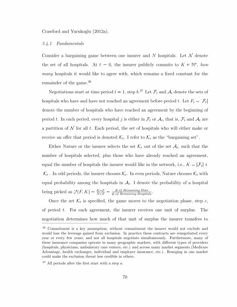
Crawford and Yurukoglu (2012a).
3.4.1 Fundamentals
Consider a bargaining game between one insurer and N hospitals. Let N denote
the set of all hospitals. At t � 0, the insurer publicly commits to K P N�, how
many hospitals it would like to agree with, which remains a fixed constant for the
remainder of the game.36
Negotiations start at time period t � 1, step b.37 Let Ft and At denote the sets of
hospitals who have and have not reached an agreement before period t. Let Ft � |Ft|
denote the number of hospitals who have reached an agreement by the beginning of
period t. In each period, every hospital j is either in Ft or At, that is, Ft and At are
a partition of N for all t. Each period, the set of hospitals who will either make or
receive an offer that period is denoted Kt. I refer to Kt as the “bargaining set”.
Either Nature or the insurer selects the set Kt out of the set At, such that the
number of hospitals selected, plus those who have already reached an agreement,
equal the number of hospitals the insurer would like in the network, i.e., K � |Ft| �
|Kt|. In odd periods, the insurer chooses Kt. In even periods, Nature chooses Kt with
equal probability among the hospitals in At. I denote the probability of a hospital
being picked as PpF,Kq � K�FN�F
� # of Remaining Slots# of Remaining Hospitals
.
Once the set Kt is specified, the game moves to the negotiation phase, step c,
of period t. For each agreement, the insurer receives one unit of surplus. The
negotiation determines how much of that unit of surplus the insurer transfers to
36 Commitment is a key assumption; without commitment the insurer would not exclude andwould lose the leverage gained from exclusion. In practice these contracts are renegotiated everyyear or every few years, and not all hospitals negotiate simultaneously. Furthermore, many ofthese insurance companies operate in many geographic markets, with different types of providers(hospitals, physicians, ambulatory care centers, etc.) and across many market segments (MedicareAdvantage, health exchanges, individual and employer insurance, etc.). Reneging in one marketcould make the exclusion threat less credible in others.
37 All periods after the first start with a step a.
70

the hospital, denoted xj. When t is odd, the insurer makes offers to all hospitals
in Kt simultaneously. When t is even, all hospitals in Kt make offers to the insurer
simultaneously. A player who receives an offer has a binary choice to either accept or
reject that offer. If the offer between hospital j and the insurer is accepted, hospital
j joins the set Ft�1 and remains in F for all subsequent periods. If an offer is rejected
at period t, that hospital joins the set At�1. The game ends when K agreements
have been made or when a breakdown occurs.
In order to have price determinacy, models of bargaining require a friction or cost
of negotiating. I include an exogenous probability of breakdown, similar to Binmore
et al. (1986). Starting in period t � 2 and in every following period, before Kt is set,
Nature determines whether a breakdown occurs. I allow hospitals and the insurer to
have asymmetric beliefs about the subjective probability of breakdown denoted by
ρHj and ρI , respectively.38 When a breakdown occurs, the game ends and no further
agreements can be made, though surplus created and transfers previously agreed to
remain. All excluded hospitals, either due to the insurer reaching K agreements
or breakdown receive zero surplus. Renegotiation of contracts is not allowed. The
breakdown probabilities are assumed to be constant throughout time and do not
vary based on which hospitals have reached agreements. Players do not discount the
future.
For clarity, I respecify the timing of the model:
t=0. Insurer publicly commits to size of their network, K.
t � 1, 3, 5, ... (if F K agreements have been reached):
38 Asymmetric beliefs are allowed for in Binmore et al. (1986), with the assumption of someappropriate behavioral model, for example heterogenous priors. I follow Binmore et al. (1986) anddo not specify this aspect of the model because it is not a key feature of the model. The main resultsof the model can be shown with symmetric beliefs. However, asymmetric beliefs help highlight theconcerns endogenous networks raise for the reduced-form analysis and are an important feature ofthe empirical model where the interpretation of this parameter is different.
71

a. (Except period t � 1) Nature decides whether there is a breakdown.
b. Insurer picks which hospitals to make an offer to K.
c. Insurer makes simultaneous offers to the hospitals in K.
d. Hospitals simultaneously decide whether to accept or reject their offer.
t � 2, 4, 6, ... (if F K agreements have been reached):
a. Nature decides whether there is a breakdown.
b. With equal probability PpF,Kq � K�FN�F
, Nature chooses K � F hospitals to
make an offer K.
c. Hospitals in K make simultaneous offers to the insurer.
d. Insurer simultaneously decides whether to accept or reject each offer.
The game stops when K hospitals have reached agreement or breakdown occurs.
Payments are made.
The structure of the game is common knowledge. Players know the surplus
functions and all the parameters. At the end of t � 0, all the players know K. At
the beginning of each period t ¡ 0, players know which players have agreed already,
Ft, and which remain active, At. During period t, once the bargaining set, Kt, has
been set but before offers are made, all players learn Kt. That is, they all know
which other hospitals are negotiating before offers are made. Because offers are
made simultaneously, hospitals do not know what offers the others made/received.
Likewise, similar to Crawford and Yurukoglu (2012a), I do not allow the insurer to use
its information about what hospitals have offered or which hospitals have accepted to
be used that period in decisions with other hospitals. That is, I rule out informational
asymmetries for the insurer. Once all offers have been made and responded to, all
players learn which agreements were reached so that at the beginning of period t� 1
the sets Ft�1 and At�1 will be known.
72
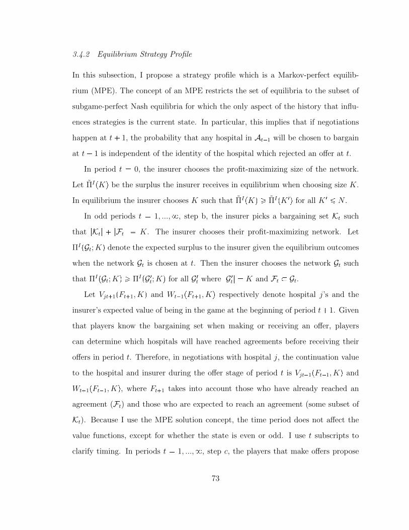
3.4.2 Equilibrium Strategy Profile
In this subsection, I propose a strategy profile which is a Markov-perfect equilib-
rium (MPE). The concept of an MPE restricts the set of equilibria to the subset of
subgame-perfect Nash equilibria for which the only aspect of the history that influ-
ences strategies is the current state. In particular, this implies that if negotiations
happen at t� 1, the probability that any hospital in At�1 will be chosen to bargain
at t� 1 is independent of the identity of the hospital which rejected an offer at t.
In period t � 0, the insurer chooses the profit-maximizing size of the network.
Let ΠIpKq be the surplus the insurer receives in equilibrium when choosing size K.
In equilibrium the insurer chooses K such that ΠIpKq ¥ ΠIpK 1q for all K 1 ¤ N .
In odd periods t � 1, ...,8, step b, the insurer picks a bargaining set Kt such
that |Kt| � |Ft| � K. The insurer chooses their profit-maximizing network. Let
ΠIpGt;Kq denote the expected surplus to the insurer given the equilibrium outcomes
when the network Gt is chosen at t. Then the insurer chooses the network Gt such
that ΠIpGt;Kq ¥ ΠIpG 1t;Kq for all G 1t where |G 1t| � K and Ft � Gt.
Let Vjt�1pFt�1, Kq and Wt�1pFt�1, Kq respectively denote hospital j’s and the
insurer’s expected value of being in the game at the beginning of period t� 1. Given
that players know the bargaining set when making or receiving an offer, players
can determine which hospitals will have reached agreements before receiving their
offers in period t. Therefore, in negotiations with hospital j, the continuation value
to the hospital and insurer during the offer stage of period t is Vjt�1pFt�1, Kq and
Wt�1pFt�1, Kq, where Ft�1 takes into account those who have already reached an
agreement (Ft) and those who are expected to reach an agreement (some subset of
Kt). Because I use the MPE solution concept, the time period does not affect the
value functions, except for whether the state is even or odd. I use t subscripts to
clarify timing. In periods t � 1, ...,8, step c, the players that make offers propose
73

the offeree’s continuation value. When t is odd, the insurer offers the hospital: xjt �
Vjt�1pFt�1, Kq. When t is even, the hospital offers (to keep): xjt � 1�Wt�1pFt�1, Kq.
The player who is offered their continuation value will accept.
Finally, I assume that in equilibrium there will be immediate agreement:
Assumption 1. Suppose the beliefs about breakdown probabilities are such that a
possible equilibrium involves immediate agreement (Kr agreements are reached in
period t � 1 for each r) and that this equilibrium is played.
In the simplified model there are two reasons why it is unprofitable for the insurer
to delay. First, as with many dynamic games of complete information delay is un-
profitable for the insurer is that the expected costs of breakdown are higher if fewer
hospitals have agreed at any point in time. Second, delay improves the continuation
value of a hospital who reaches an agreement at t � 1 because the probability they
are picked again if they deviate is higher than when all hospitals agree at period
t � 1.39 Recall that P � K�FN�F
. Because K ¤ N , this probability is decreasing in F .
Consider, for example, when N � 9 and K � 3. If F2 � 1, (one hospital has already
agreed at the beginning of period 2), P � .25 (2 slots left divided by 8 hospitals left).
If F2 � 2, then P � .14 (1 slot left divided by 7 hospitals left).
3.4.3 Determining Continuation Values
Now, I discuss the equilibrium outcomes and compute the continuation values, given
the strategies specified in the previous section. While all hospitals agree in the first
period, continuation values depend on the expected value for hospital j after deviat-
ing from the equilibrium and rejecting the offer. Deviating hospital j’s expected value
for period t � 2, given equilibrium strategies and immediate agreement, simplifies
39 This is a similar argument to Moller (2007) who argues that when the timing of agreementsis endogenous, there is an incentive for simultaneous agreements when the externalities betweenplayers weakens over time.
74

to:
Vjt�2pK � 1, Kq � p1 � ρHj q �PpK � 1, Kq � r1 �Wt�3pK � 1, Kqs � ρHj � 0 (3.1)
With probability ρHj , breakdown occurs and the hospital gets nothing. With prob-
ability p1 � ρHj q, agreements are made possible in period t � 2. In period t � 2,
with probability P � 1N�K�1
, hospital j will be chosen to make an offer. Because
in equilibrium, all hospitals reach an agreement at t � 1, in considering the value of
deviating, hospital j expects the set of hospitals who have reached an agreement will
consist of all the hospitals in the original bargaining set except itself, i.e., F2 � K�1.
It offers the insurer its continuation value for period t � 3 and keeps the remainder.
The input to Wt�3pK � 1, Kq is pK � 1, Kq because again we are considering a case
where the insurer deviates to determine the continuation value.
Now I solve for the insurer’s continuation value by considering the case where it
deviates at period t � 2. The insurer’s expected value in t � 3, given that the K � 1
hospitals have agreed is:
Wt�3pK � 1, Kq � p1 � ρIq r1 � Vjt�4pK � 1, Kqs � ρI � 0 (3.2)
With probability ρI , breakdown occurs and the insurer gets nothing from this hos-
pital, so it receives the values from other agreements (which I omit because they
are sunk). With probability p1 � ρIq, the game goes forward and the insurer offers
hospital j its continuation value.
3.4.4 Bargaining Results
To calculate transfers, I consider a unilateral deviation by each hospital j P K1
separately. Because of immediate agreement, a unilateral deviation would imply
there is only one additional agreement remaining. At this point the state of the
game does not change from period t � 2 until an agreement is reached (conditional
75

on the state being even or odd). Because the value functions only depend on the
state, and the state only depends on whether the time is even or odd, Vjt�2pK �
1, Kq � Vjt�4pK � 1, Kq � ... � Vj evenpK � 1, Kq and likewise for Wt�3pK � 1, Kq �
Wt�5pK � 1, Kq � ... � WoddpK � 1, Kq. Therefore, for each insurer-hospital pair
there are two unknowns (Vj evenpK � 1, Kq and WoddpK � 1, Kq) and two equations
linear in the unknowns, so there exists a unique solution that can be represented
with a closed form. Proposition 1 presents this solution:
Proposition 1. The equilibrium outcome of this game is given by:
xjpKq �ρI � rp1 � ρHj q �
1N�K�1
s
1 � p1 � ρIq � rp1 � ρHj q �1
N�K�1s
Relationship to Rubinstein Outcomes
Corollary 2 states that when K � N , meaning the insurer chooses not to exclude,
the model predicts N outcomes that match the outcomes in Rubinstein (1982).40 In
particular, K � N implies that Pp�q � 1, i.e., hospitals who reject an offer in the
previous period will be picked with probability one. The solution reduces to:
Corollary 2. When K � N and Pp�q � 1, the equilibrium outcome simplifies to:
xjpNq �p1 � ρHj q � ρ
I
1 � p1 � ρHj q � p1 � ρIq
Allowing for exclusion, the results are the same as Rubinstein (1982), except that
the hospitals’ risk of breakdown parameters are multiplied by their probability of
being chosen, as highlighted by the brackets in Proposition 1. One way to inter-
pret this is that my result is distinguishing the risk of breakdown from the risk of
40 Technically these are Binmore et al. (1986) outcomes because the cost of negotiation is modeledas a risk of breakdown. However, the result would be the same as Rubinstein (1982) if I modeled itas a discount factor. I cite Rubinstein (1982) since it may be more familiar to a broader audience.
76

exclusion due to the narrow-network. This also demonstrates how my model nests
the Nash-in-Nash solution. When there is no exclusion (or the probability of being
picked after deviating equals 1), each negotiation becomes the outcome of a pairwise
Rubinstein bargain, conditional on all the other negotiations. Collard-Wexler et al.
(2016) provides sufficient conditions under which this limits to the Nash-in-Nash
solution, similar to how Binmore et al. (1986) demonstrates that Rubinstein (1982)
limits to the Nash solution. The remaining results show how my model extends the
Nash-in-Nash model.
Narrow-Networks Negotiate Smaller Transfers
My next result shows that my model can imply smaller transfers when there is
exclusion. This is a straightforward consequence of Proposition 1. Intuitively, the
reason this occurs is that by excluding, the insurer is increasing the probability the
hospital gets zero, which worsens the hospital’s continuation value. Why this worsens
the continuation value is clear from Equation 3.1, as the value function is multiplied
by PpK�1, Kq � 1N�K�1
. If hospital j disagrees when many hospitals are excluded,
the probability it gets nothing p1� 1N�K�1
q is large. When few hospitals are excluded,
the probability of getting nothing is smaller, so the continuation value is larger.
While it may be intuitive that exclusion leads to smaller transfers, it is not obvious
that exclusion can be optimal for the insurer. By narrowing the network, the insurer
reduces total surplus, which would not be optimal if it did not get larger transfers.41
Exclusion in Equilibrium
Figure 3.1 plots the value function at the beginning of the game for the insurer
given different choices of K. I assume all hospitals have the same risk of breakdown
probabilities. There are 7 hospitals in this game. ρI � .75, so the insurer expects
41 In my empirical setting, consumers prefer larger networks (more choice of hospitals, etc.) so abroad-network can charge higher premiums.
77

a non-degenerate risk of breakdown. The top line, ρH � 1, shows that when the
hospitals do not expect to have a chance to offer, and thus have no bargaining
power, the insurer receives all the surplus. In this case, the insurer agrees with all 7
and they create 7 units of surplus which are all kept by the insurer. When ρH � .25,
the insurer excludes 1 hospital in equilibrium, creating 6 total units of surplus and
keeps roughly 4 of these units. If it were to choose K � 7, it would create 7 total
units of surplus, but would only keep 2 of these units. Finally, when ρH � 0, the
insurer will exclude two hospitals. Instead, if it were to exclude no hospitals, the
hospitals would capture all the surplus. The K � N case matches the Rubinstein
outcome (Corollary 2) times N , which is often not optimal for the insurer.
Figure 3.1: Insurer’s t � 0 expected value by network size.
Results are from simulated data, using the following parameters:ρI � .75, ρH � .25,Π � 1, N � 7
Finally, I discuss the endogeneity concern my model raises. In Figure 3.1, the
insurer’s risk of breakdown parameter is fixed at ρI � .75. As ρH increases, the
insurer excludes fewer hospitals. This demonstrates that, as the insurer’s relative
bargaining power increases, it is less likely to exclude.42 Intuitively, an insurer that
42 This result is also shown in Gal-Or (1999).
78

will get less of the pie will not be affected as much by shrinking that pie. This raises
a concern about selection into network size. If plans that are unable to negotiate low
prices are the most likely to use the tool of exclusion, then observed broad-network
prices are not an appropriate comparison. In Figure 3.1, when ρH � 0, the insurer
chooses to exclude two hospitals, but if it had a broad network, it would transfer the
entire unit of surplus to hospitals. In the other extreme, when ρH � 1, the insurer
transfers no surplus to the hospitals.
3.5 Structural Model and Estimation
The estimation strategy amounts to matching the split of surplus predicted by the
model to the “observed split of surplus.” While estimation of games with endogenous
networks can be challenging, the key insight of this section is that estimation of a
game with simultaneous agreement makes estimation feasible. This is a feature of the
Nash-in-Nash model; however, it is not standard in the literature where prices and
the networks are endogenous, which uses randomly ordered sequential matching. I
begin by discussing how I estimate the surplus over which the hospitals and insurers
negotiate. Then I discuss how I estimate the bargaining parameters.
There are two important distinctions between the theoretical model and the em-
pirical model. I allow for hospitals and insurers to negotiate over a linear prices
and the interpretation of the risk of breakdown parameter changes. I back out the
linear price that is consistent with the lump-sum transfer that is implied by the
model. This is also done in Gowrisankaran et al. (2014), Ho and Lee (2017), and
Prager (2016). Since I do not observe the price for each hospital-insurer-service com-
bination, I assume that insurers negotiate a constant markup above a CPT4 code’s
relative weight. Throughout the paper, I refer to lump-sum payments as transfers
and payments based on a linear price schedule as prices.43
43 For those who have read the appendix, I change notation from x, which represents transfers, to
79

In the previous theory section, the cost of negotiation is represented by an ex-
ogenous risk of breakdown due to the regulator ending the game. This parameter
explains how surplus is split between parties and therefore is often referred to as a
“bargaining parameter.” In the empirical literature, the bargaining parameters are
estimated as the residuals that explain the split of surplus beyond other aspects of
the model and data. That is, the bargaining parameters are interpreted as reduced-
form parameters which explain how surplus is divided between hospitals and insurers.
This does not preclude the risk of breakdown as an aspect of price formation, but
accounts for many other stories (for which data are not available) that effect price
formation.
3.5.1 Defining Surplus
In order to estimate the bargaining model from the previous section, I require esti-
mates of the surplus at stake in each negotiation. Surplus is defined as the sum of
profits to each insurer and the providers they contract with, which are determined
by consumers’ choices over which hospitals to use and which plans to enroll in. This
allows insurers’ valuation of hospitals to depend on how its enrollees value those
hospitals. This section presents a five-stage model which describes how consumers
make these choices, how the insurers set their premiums, and how prices and the
network are negotiated.
Stage 1: Prices and the network are negotiated between insurers and hospitals.
Stage 2: Insurers set their premiums.
Stage 3: Consumers choose which health plan to join.
Stage 4: Nature determines which consumers get sick.
Stage 5: Consumers who got sick choose which hospital to attend.
Besides the bargaining stage, the framework in this section is standard in the lit-
p, which represents prices.
80
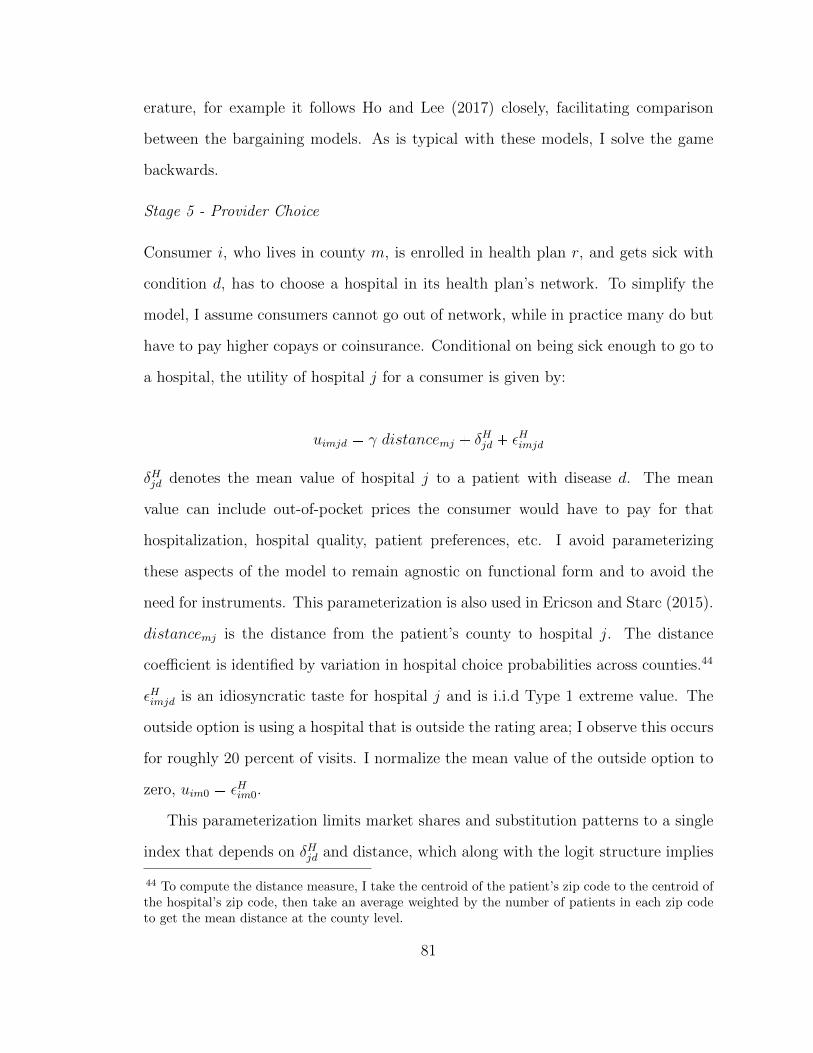
erature, for example it follows Ho and Lee (2017) closely, facilitating comparison
between the bargaining models. As is typical with these models, I solve the game
backwards.
Stage 5 - Provider Choice
Consumer i, who lives in county m, is enrolled in health plan r, and gets sick with
condition d, has to choose a hospital in its health plan’s network. To simplify the
model, I assume consumers cannot go out of network, while in practice many do but
have to pay higher copays or coinsurance. Conditional on being sick enough to go to
a hospital, the utility of hospital j for a consumer is given by:
uimjd � γ distancemj � δHjd � εHimjd
δHjd denotes the mean value of hospital j to a patient with disease d. The mean
value can include out-of-pocket prices the consumer would have to pay for that
hospitalization, hospital quality, patient preferences, etc. I avoid parameterizing
these aspects of the model to remain agnostic on functional form and to avoid the
need for instruments. This parameterization is also used in Ericson and Starc (2015).
distancemj is the distance from the patient’s county to hospital j. The distance
coefficient is identified by variation in hospital choice probabilities across counties.44
εHimjd is an idiosyncratic taste for hospital j and is i.i.d Type 1 extreme value. The
outside option is using a hospital that is outside the rating area; I observe this occurs
for roughly 20 percent of visits. I normalize the mean value of the outside option to
zero, uim0 � εHim0.
This parameterization limits market shares and substitution patterns to a single
index that depends on δHjd and distance, which along with the logit structure implies
44 To compute the distance measure, I take the centroid of the patient’s zip code to the centroid ofthe hospital’s zip code, then take an average weighted by the number of patients in each zip codeto get the mean distance at the county level.
81

the independence of irrelevant alternatives (IIA) property. Also, if patients of dif-
ferent health status choose hospitals differently, as shown in Shepard (2016), then
my model would overestimate the value (to the insurer) of hospitals that attract
the costliest patients. In order to account for these concerns, I include age-hospital
interactions to allow individual’s preferences for hospitals to vary by age as well.
I estimate hospital choice parameters by inverting the age-gender-county-condition
specific market shares and running OLS, as shown in Berry (1994). Because of the
distributional assumption of εHimjd, the expected probability of going to a hospital, in
a particular plan, conditional on a consumer getting sick is:
σimjdpFrq �exp
�γ distancemj � δHjd
�1 �
°kPFr
exp pγ distancemk � δHkdq
Stage 4 - Nature Determines Which Consumers Get Sick
In stage 4, there are no strategic decisions to be made, as Nature determines which
consumers get sick. Let the probability of getting sick with disease d be given by fid.
I calculate fid by using the observed probability that an enrollee has a hospital visit,
for disease d, in my sample. I compute the number of enrollees in 12 groups, (six age
categories times gender).45 I estimate this probability across the entire rating area.
Stage 3 - Consumers Choose health plans
In stage 3, consumers choose their health plan. Following Town and Vistnes (2001)
and Capps et al. (2003), I model utility as the value of premiums, the expected value
of the network, and other plan characteristics:
Uimr � α1r premiumir � α2 Epuimrq � ξmr � εPimr
45 Age categories are: 0-18, 19-25, 26-35, 36-45, 46-55, 56-65
82

premiumir is the premium that consumer i would face, which is, by law, constant
across counties within a rating area, except by age. ξmr is other unobserved plan
characteristics which can vary by county. εPimr represents idiosyncratic consumer
preferences over plan characteristics that are assumed to be i.i.d Type 1 extreme
value. α1r is a health plan specific premium-sensitivity parameter. Epuimrq is the
expected utility of the providers in health plan r’s network. This is also referred to
as willingness to pay (WTP) for the network46 This value, as shown in Capps et al.
(2003) is given by the familiar inclusive value formula, incorporating the probability
of getting sick with disease d:
Epuimrq �¸dPD
fid ln� ¸jPFr
exppγ distancemj � δHjdq�
Prager (2016), Ericson and Starc (2015), and Ho and Lee (2017) use variation in
premiums offered for individual versus family plans to account for the endogeneity
of premiums. My data does not have information on which enrollees are in which
families. Furthermore, many enrollees receive unobserved subsidies for premiums,
which creates measurement error in the observed premium that is paid by an enrollee.
To handle these concerns, rather than estimating α1r directly, I back out α1r using
first-order conditions implied by optimal premium setting.47 This similar to how
Rosse (1970) or Berry (1994) use optimal pricing to back out marginal costs. First,
I estimate α2 separately by defining δPimr � α1rpremiumr � ξmr as the mean value of
the plan, net of the value of the network in each county. Then I rewrite the utility
function as:
46 This varies from the rest of the literature; because I do not estimate the copay sensitivity, I donot rescale the WTP term. Therefore, it is measured in units of utils, rather than dollars.
47 The supply-side premium elasticity is more relevant because the main purpose of this stage isto understand how insurers update premiums. This also avoids the measurement concern due tosubsidies. While I have not computed welfare results, I will need to account for consumers facingdifferent premiums.
83

Uimr � α2 Epuimrq � δPimr � εimr
I estimate α2 by inverting the market shares for each plan, in each county, for each
demographic group. There are two sources of identifying variation: consumer de-
mographics and geographic variation. Each demographic group values the network
differently, so if those who value networks more (typically older patients) choose
broader networks, one would expect a positive α2. Likewise, plans vary in terms of
the location of their in-network hospitals. α2 will be positive if consumers are more
likely to choose plans which include nearby hospitals. The outside option is being
uninsured. I use the estimates from Panhans (2016), who calculates the insurance
take-up rate by age in Colorado. The uninsured rate varies from 30 percent to 60
percent, mostly declining by age.48
Denote the probability that consumer i, in county m, signs up for insurance plan
r as SimrppremiumpF , pq,Fq. F represents the set of all observed networks. The
functional form is due to the distributional assumption on εPimr:
Simrppremium,Fq �exp pα1r premiumir � α2 Epuimrq � ξrq
1 �°kPR exp pα1k premiumik � α2 Epuimkq � ξkq
(3.3)
Because the market shares take into account premiums and networks from each
insurer in the market, I omit the r subscript on premium and F . This equation
defines how cross-insurer competition is accounted for in the model; plans engage in
Nash-Bertrand competition over premiums, after the networks and prices are set.
48 Under the ACA regulations, there is an “individual mandate” that requires all individuals eligiblefor the exchanges to have insurance. In 2014, those who do not purchase insurance and were notexempt were liable for a “shared responsibility payment” of $95 or one percent of household income,whichever was greater for an individual.
84

Stage 2 - Insurers Choose Premiums
Insurer r’s expected profits consist of the premiums it receives, minus the expected
amount it must reimburse the hospitals in its network. The expected amount it must
pay for consumer i is the probability of the consumer being sick with disease d pfidq
times the expected value of the payments (weighted by the probability of going to
each hospital, conditional on having disease d, p°jPFr
pjdrpF ,Πr, KqσimjdpFrqq times
the probability that the consumer chooses that health plan pSimrppremiumpF , pq, Fqq.
ΠIrpF , p,Kq �
¸i
�premiumirpF , prq �
¸dPD
fid
¸jPFr
pjdrpF ,Πr,Kq � σimjdpFrq � other costsi
�
(3.4)
� SimrppremiumpF , pq, Fq
I also include other costsi that account for each consumer’s expected costs for the
insurer in other settings, such as inpatient hospitals and physician visits. To back
out plan-specific premium sensitivities, α1r, I take the derivative of Equation 3.4
with respect to premiums. I solve for it α1r, since all other terms in this equation
are observed or estimated. I use the estimated market share values, since the model
suggests that plans set premiums based on expected costs not observed costs.
3.5.2 Stage 1 - Providers and Insurers Bargain over Prices and the Network
For the remainder of the paper, I refer to the subjective beliefs about the risk of
breakdown, ρHj and ρIr, as “generic bargaining parameters” to differentiate the bar-
gaining power they provide from the threat of exclusion and highlight how all other
sources of bargaining power are accounted for in these parameters. In this section,
I discuss the estimation of the generic bargaining parameters, ρHj and ρIr, and the
effect of exclusion Pr. While I have focused on the effect of exclusion, the generic
bargaining parameters are relevant for network adequacy policies as well. If hospi-
tals have a lot of relative bargaining power, then restricting one of the insurer’s tools
85

to gain leverage may raise prices a lot. On the other hand, if insurers have a lot
of relative bargaining power, even without the use of exclusion, then these policies
would not impact prices much.
To estimate these parameters, I match the model’s prediction of the split of
surplus to the observed split of surplus. The observed split of surplus is the hos-
pital’s profits divided by the marginal surplus hospital j contributes to network r,
pΠMARGjr pF ,Frztju, ppFq, Kqq. The marginal surplus contains three terms: (1) the
surplus the insurer receives with the observed network pΠIrpF , p,Kqq (2) the surplus
captured by hospital j, given the observed network pΠHjrpF , p,Kqq (3) minus the sur-
plus the insurer would obtain if they made offers to the observed network, but hospi-
tal j (and only hospital j) deviates, followed by a breakdown pΠIBjr pF ,Frztju, ppFq, Kqq.
Formally, the marginal surplus can be written:
ΠMARGjr pF ,Frztju, ppFq, Kq � ΠI
rpF , p,Kq�ΠHjrpF , p,Kq�ΠIB
jr pF ,Frztju, ppFq, Kq
(3.5)
Note that marginal surplus is not a value that I am assuming, but rather this is
derived in the appendix.49
The surplus captured by the insurer, pΠIrpF , p,Kqq, is given in Equation 3.4. The
surplus captured by hospital j from insurance company r is defined as the price that
the hospital receives for each service minus the marginal cost of the service, times
the number of services the hospital provides. The number of services is defined as
the probability of patient i joining insurer r’s plan, times the probability of being
sick with disease d, times the probability of using hospital j, conditional on having
disease d:
49 Due to the linearity of the surplus functions, this is an equivalent way of writing the equationin the appendix. ΠI
r � Πr �°
ΠHir , then I add back in ΠH
jr because it is not subtracted off.
86
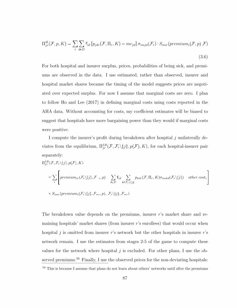
ΠHjrpF , p,Kq �
¸i
¸dPD
fid rpjdrpF ,Πr, Kq �mcjdsσimjdpFrq �SimrppremiumipF , pq Fq
(3.6)
For both hospital and insurer surplus, prices, probabilities of being sick, and premi-
ums are observed in the data. I use estimated, rather than observed, insurer and
hospital market shares because the timing of the model suggests prices are negoti-
ated over expected surplus. For now I assume that marginal costs are zero. I plan
to follow Ho and Lee (2017) in defining marginal costs using costs reported in the
AHA data. Without accounting for costs, my coefficient estimates will be biased to
suggest that hospitals have more bargaining power than they would if marginal costs
were positive.
I compute the insurer’s profit during breakdown after hospital j unilaterally de-
viates from the equilibrium, ΠIBjr pF ,Frztju, ppFq, Kq, for each hospital-insurer pair
separately:
ΠIBjr pF ,Frztju, ppFq,Kq
�¸i
��premiumirpFrztju,F�r, pq �
¸dPD
fid
¸kPFrztju
pkdrpF ,Πr,KqσimkdpFrztjuq � other costi
��
� SimrppremiumipFrztju,F�r, pq, Frztju,F�rq
The breakdown value depends on the premiums, insurer r’s market share and re-
maining hospitals’ market shares (from insurer r’s enrollees) that would occur when
hospital j is omitted from insurer r’s network but the other hospitals in insurer r’s
network remain. I use the estimates from stages 2-5 of the game to compute these
values for the network where hospital j is excluded. For other plans, I use the ob-
served premiums.50 Finally, I use the observed prices for the non-deviating hospitals:
50 This is because I assume that plans do not learn about others’ networks until after the premiums
87
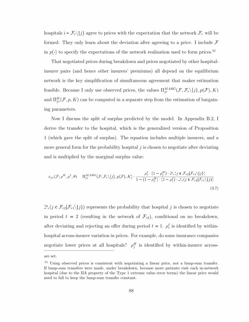
hospitals i P Frztju agree to prices with the expectation that the network Fr will be
formed. They only learn about the deviation after agreeing to a price. I include F
in pp�q to specify the expectations of the network realization used to form prices.51
That negotiated prices during breakdown and prices negotiated by other hospital-
insurer pairs (and hence other insurers’ premiums) all depend on the equilibrium
network is the key simplification of simultaneous agreement that makes estimation
feasible. Because I only use observed prices, the values ΠMARGjr pF ,Frztju, ppFq, Kq
and ΠHjrpF , p,Kq can be computed in a separate step from the estimation of bargain-
ing parameters.
Now I discuss the split of surplus predicted by the model. In Appendix B.2, I
derive the transfer to the hospital, which is the generalized version of Proposition
1 (which gave the split of surplus). The equation includes multiple insurers, and a
more general form for the probability hospital j is chosen to negotiate after deviating
and is multiplied by the marginal surplus value:
xjrpF ; ρH , ρI , θq � ΠMARGjr pF ,Frztju, ppFq,Kq �
ρIr � p1 � ρHj q �Prpj P Fr2|Fr1ztjuq
1 � p1 � ρHj q � p1 � ρIrq �Prpj P Fr2|Fr1ztjuq
(3.7)
Prpj P Fr2|Fr1ztjuq represents the probability that hospital j is chosen to negotiate
in period t � 2 (resulting in the network of Fr2), conditional on no breakdown,
after deviating and rejecting an offer during period t � 1. ρIr is identified by within-
hospital across-insurer variation in prices. For example, do some insurance companies
negotiate lower prices at all hospitals? ρHj is identified by within-insurer across-
are set.
51 Using observed prices is consistent with negotiating a linear price, not a lump-sum transfer.If lump-sum transfers were made, under breakdown, because more patients visit each in-networkhospital (due to the IIA property of the Type 1 extreme value error terms) the linear price wouldneed to fall to keep the lump-sum transfer constant.
88

hospital variation, conditional on those hospital’s marginal surplus. For example, do
certain hospitals negotiate higher prices across all insurance companies, conditional
on the marginal surplus they provide? That negotiated prices are not included in
the estimation of other stages helps to clarify the variation in the data that identifies
these parameters.
One difference between my model and the Nash-in-Nash model is that hospi-
tals which are excluded from the network may have an effect on hospitals who are
included. Town and Vistnes (2001) describes why excluded hospitals may affect a
hospital’s bargaining leverage: “With HMOs contracting with multiple hospitals to
form networks, a hospital’s bargaining leverage depends both on its own characteris-
tics and on the characteristics of other hospitals inside and outside the network. In
particular, if the HMO’s best alternative to contracting with a high-priced hospital is
to replace that hospital with another, the high-priced hospital’s bargaining leverage
depends on the hospital’s incremental value to the network relative to other hospi-
tals that could replace it.” This is incorporated into my theoretical model through
the probability of being picked after deviating. If hospital j’s probability of being
picked in the period after deviating is affected by how many (or which) hospitals are
excluded, then that would effect the continuation value of hospital j.
However, the probability of being chosen to make an offer after deviating is not
observable, since by definition it does not occur in equilibrium. This may require
a more complete model of network formation which might depend on factors like
insurers’ interactions with hospitals in other markets (e.g., does an insurer contract
with a hospital in a plan it offers in its employer-sponsored insurance or its Medicare
Advantage line of business?) and dynamic factors (e.g., did its network include that
hospital in previous years?). While an interesting avenue of research, I consider this
outside the scope of this paper.
The assumption of hospitals being chosen with equal probability after deviating is
89

arbitrary and likely to be an unrealistic measure of the competitive effect of excluded
hospitals. Therefore, in some specifications, I include a reduced-form parameter, θ,
which captures the correlation between the substitutability of excluded hospitals
and the negotiated prices of hospitals in the network. I also present a specification
without this parameter, since it is not structural parameter.
To measure the substitutability of excluded hospitals, I calculate the number of
“acceptable replacement” hospitals that are excluded from the observed network but
would provide sufficient surplus to be able to reach an agreement with the insurer
after a hospital in the observed network deviates. For example, in a market where
hospitals A and B are within one mile of each other and hospital C is fifty miles away,
an insurer may only need one of A and B, but require C. Suppose the insurer selects
tA,Cu; then if C deviates, it will have probability one of being picked again, while
A has a one-half probability of being picked because B is an acceptable replacement
for it.
Given the number of acceptable replacement hospitals, I parameterize the prob-
ability of hospital j being selected after deviating with insurer r as follows:
Prpj P Fr2|Fr1ztju; ρH , ρI , θq � exppθ � logpPrpj P Fr2|Fr1ztju; ρH , ρIqq
where Prpj P K2|K1ztju; ρH , ρIq represents the equal probability chance of being
picked to offer after deviating, which is one divided by the number of acceptable
hospitals plus one for hospital j itself. The advantage of this functional form is, if
there are no replacement hospitals (i.e., if this is a broad-network), then P � 1,
because P � 1 (and logpPq � 0). If P 1 and θ � 0, then P � 1 and there is
no correlation between negotiated price and the number of excluded hospitals. If
P 1 and θ � 1, then P � P, which is consistent with the naive assumption of
equal probability among acceptable hospitals. θ P p0, 1q implies a correlation between
these two extremes.
90

θ captures the reduced-form effect of having excluded hospitals that are close
substitutes. θ is identified by variation in the number of acceptable replacement
hospitals which may vary across hospitals within a network, as in the case of hos-
pitals tA,Cu given above. That is, this parameter is identified by variation in each
in-network hospital’s characteristics and how they compare to excluded hospitals,
conditional on the observed networks. To test the sensitivity of this parameter, I
present four parameterizations. (1) I do not include this parameter. (2) I include
one θ which does not vary across hospital-insurer pairs. (3) I include an insurer-
specific θr. (4) I include a hospital-specific θj.52 Including an insurer-specific θr
might be preferred if certain insurers can use the threat of exclusion more effectively
than others. For example, if they contract with a hospital in another market, such
as the employer-sponsored insurance market, the threat of exclusion may carry extra
weight or other hospitals may be worse substitutes than implied by the model. Like-
wise, a hospital-specific θj may be preferred if certain hospitals are more difficult to
exclude. For example, a star hospital may not be a close substitute for others. The
reduced-form parameter would capture these effects. I leave the details of computing
the number of acceptable replacement hospitals to Appendix B.3.
To estimate this model once I have computed Prpj P Kr2|Kr1ztju; ρH , ρI , θq, for
that draw of parameters, I can compute the transfer implied by the model:
xjrpF ; ρH , ρI , θq
ΠMARGjr pF ,Frztju, ppFq, Kq
where xjrpF ; ρH , ρI , θq is given by Equation 3.7 (except using P). I find the set of
parameter values ρH , ρI , θ that minimize the distance between the model-predicted
52 I cannot include a θjr because the variation needed to identify this parameter is based on eitherwithin-hospital or within-insurer variation in the number of acceptable replacement hospitals.
91

split of surplus and the observed split of surplus given by:
ΠHjrpFq
ΠMARGjr pF ,Frztju, ppFq, Kq
3.6 Results
This section presents the estimation results of my model. I show that consumers
value closer hospitals, broader networks, and lower premiums, as expected. The main
point of these results are that they are all similar to those in the literature, which
facilitates the comparison of the bargaining models. Then I discuss the estimation
results for the bargaining parameters, which are the focus of this paper. I present
results for the model with and without allowing for exclusion. I use these results
in the counterfactual and use the counterfactual to aid the interpretation of the
bargaining parameters.
3.6.1 Demand Estimation Results
In Stage 5, consumers who got sick choose which hospital to attend. Table 3.5 shows
the results of the hospital demand regressions. The first column does not include
age-hospital interactions, while the second does. In both, the coefficient on distance
in miles is roughly �0.016. This implies an elasticity of �0.16, meaning that a
one-percent increase in distance to a hospitals leads to a .16 percent lower chance
of attending that hospital. The negative coefficient on distance is common in the
literature, for example Town and Vistnes (2001), Prager (2016), and Ho and Lee
(2017) all find negative coefficients on distance.
In Stage 4, Nature decides which consumers get sick and what conditions they get.
I determine the probability of being treated for condition d for a given gender-age
group. Table 3.6 presents the probability of an individual being treated for condition
d. Injuries, diseases of the musculoskeletal system, and neoplasms were the most
92

common conditions.53 Roughly 2.25 percent of the sample had an outpatient visit in
2014 for an injury, and 1 percent for neoplasms. Table 3.7 presents the probability
of having a hospital visit by age category. The probability of having a condition is
rising in the age of the patient. A person age 56-65 has an average of .2 hospital
visits.
In Stage 3, consumers choose their health plans, based on the premiums, net-
works, and other plan characteristics. I present results for the willingness to pay
(WTP) for the networks first, since it was estimated separately. Table 3.8 presents
summary statistics on the WTP measure. The first row shows the mean WTP for all
plans, then breaks out WTP for narrow and broad-network plans. Narrow-network
plans have lower WTP than broad-network plans since they have fewer hospitals.
The later rows show WTP by age group. Older patients have higher WTP because
they are more likely to get sick, and, conditional on getting sick, they are more likely
to use popular hospitals.
Table 3.9 presents the results for the WTP for the network. The coefficient is a
statistically significant .5, which corresponds to an elasticity of .09. This coefficient is
of the expected sign, which Prager (2016), Ho and Lee (2017), and Ericson and Starc
(2015) find as well. Since I did not estimate a copay elasticity, the interpretation
differs from the other papers in the literature, as I do not rescale the WTP measure
into dollars.
Table 3.10 presents the insurer-specific premium sensitivities. The second column
provides an indicator for whether that plan had a broad or narrow network. The
third column presents the parameter estimates, that are all between �.0009 and
�.00025. I also present elasticities because the parameter estimates are difficult to
interpret. Each consumer type (defined by their age-gender-county) will have their
53 Neoplasms are abnormal growths of tissue. Much of the spending in this category is associatedwith cancer.
93
own elasticity since the market share of each plan varies by type. The fourth column
presents the unweighted across-types mean market share-premium elasticity for each
insurer. The market share-premium elasticities are all between �1.5 and �3. These
results in line with the literature, Ho and Lee (2017) find �1.2, Cutler and Reber
(1998) find �2 and Prager (2016) finds from �.4 to �.6. The elasticities may be
larger than others in the literature due to fiercer competition in this market; the
Colorado market has more insurers than any of the other papers cited.
3.6.2 Bargaining Estimation Results
Table 3.11 and Table 3.12 list the generic bargaining parameter results for each hos-
pital and insurer, respectively. The specification I report uses the insurer-specific θr,
though the qualitative results in this section do not change based on the specification
I use. In each table, I present the model assuming the networks are endogenously and
exogenously formed. Assuming the networks are exogenous in this case is equivalent
to setting P � 1.
Because the model assumed the generic bargaining parameters represent subjec-
tive beliefs about the risk of breakdown, larger values correspond to less bargaining
power. The level of the parameters are difficult to interpret, transfers depend on an
insurer’s parameter relative to a hospital’s parameter. In both tables when exclusion
is assumed endogenous the generic bargaining parameters are larger, but for narrow-
network plans the magnitude of that difference is much larger than for broad-network
plans or hospitals. The model with exogenous exclusion overstates narrow-network
plans’ relative bargaining power, because a narrow-network plan’s use of the threat of
exclusion is accounted for in its generic bargaining parameter; their strategic choice
is being treated as a characteristic of the plan.
To aide the interpretation of the generic bargaining parameters, the fifth and sixth
columns of Table 3.12 present the split of surplus assuming P � 1 for both models. I
94
use hospital 6 and plug the parameters into Equation 3.7 (and set ΠMARGjr � 1). This
shows how the endogenous and exogenous models differ in how they split surplus,
as only determined by the generic bargaining parameters. The broad-network plans
have similar splits of surplus across both models, while the narrow-network plans
have much larger transfers for the model with endogenous networks.
Table 3.13 presents the results for the insurer-specific θr values. I still need
to compute standard errors. All the values are closer to .5 than 0 or 1. If these
values are statistically different than 0, that would suggest that insurer-hospital
pairs negotiate lower prices when there are more acceptable replacement hospitals
excluded from that insurer’s network. This would provide some evidence of a negative
correlation between the number of substitutable hospitals and negotiated prices. If
the parameter estimates are statistically different than 1, that would suggest that
equal probability of choosing replacement hospitals is too extreme. To interpret the
coefficients, consider the case with three acceptable replacement hospitals. Including
the deviating hospital implies an equiprobability value of P � .25. When θ � .5, the
implied probability would be P � .75.54 I use the counterfactual analysis to interpret
the magnitude of this effect.
3.7 Counterfactuals
Throughout this paper I have argued that exclusion is an important aspect of com-
petition in health care markets. In this section I show how incorporating exclusion
into the model can produce different counterfactual estimates than the Nash-in-Nash
model. The counterfactual I compute is that there is a law that restricts exclusion,
so each insurer chooses to have a broad network. I assume that breakdown under the
54P � expp.5 � logp.25qq.
95

counterfactual is to simply have one deviating player be excluded.55 Unlike in esti-
mation, this requires computing counterfactual prices. I compute new prices, then
update the surplus values and repeat in a fixed-point algorithm. I do this for both
endogenous and exogenous networks. In the counterfactual, P � 1 because there are
no longer acceptable replacement hospitals.
Table 3.14 presents the ratio of prices before and after the law, at hospitals
included in the observed networks. These results do not include the effect of shifting
patients to different hospitals. That is, the results should be interpreted as the mean
change in price for the same services at the same hospital, similar to the reduced-
form analysis. In the model where the networks are assumed exogenous, if the
marginal surplus is constant, the prices will remain constant; the generic bargaining
parameters are held fixed, while the other two determinants of prices, the threat of
exclusion and the marginal surplus, are assumed constant. However, the marginal
surplus declines in the counterfactual, because the insurer is distributing its patients
across more hospitals. In the counterfactual the model with exogenous networks has
36 percent lower prices.
In the model with endogenous networks, while the marginal surplus falls, the
insurers also lose the bargaining leverage due to exclusion in the counterfactual.
The difference between the columns demonstrates the magnitudes of the effect of
bargaining leverage. The first row presents the case that θ � 1, which assumes that
hospitals are chosen with equiprobability by Nature. In this case the endogenous
exclusion result suggests prices will rise by 110 percent due to the law. The second
row shows when there is one common θ for all hospitals and insurers. The third and
fourth rows show when there are insurer- and hospital-specific θ values. All three
55 If exclusion is not allowed, then an insurer might not be allowed to market their plan underbreakdown. However, this makes marginal surplus very large for each negotiation (as the hospitalscan destroy all of the insurer’s profit). This has a large effect on broad-network plans, which is anunrealistic feature of that counterfactual and distracts from the analysis of bargaining power.
96

rows show prices rising roughly 50 percent under the counterfactual law. I believe
these results are overstated because I have not yet accounted for hospital marginal
costs. This overstates hospital bargaining power, because they appear to have larger
profits. Removing the threat of exclusion increases prices for hospitals with a lot
of bargaining power more than those with little bargaining power who would not
negotiate high prices even without exclusion.
To summarize, I have showed that restricting insurers’ ability to exclude hospitals
may lead to higher negotiated prices, which is in line with conventional wisdom. I am
still working on a full welfare analysis, but the results for negotiated prices suggest
that restricting insurers’ ability to exclude may raise premiums for consumers and
potentially hurt welfare, in some settings.
3.8 Limitations and Extensions
I believe the main limitation of this paper is how it accounts for the benefits of a
network adequacy policy (in the welfare analysis I plan to provide). Regulators worry
that consumers, not knowing which conditions they will get in the following year,
will not account for these diseases when choosing a plan. A thorough welfare analysis
of network adequacy policy should account for the fact that consumers often do not
search over providers, do not account for uncertainty in the way my model assumes,
and provider lists are often wrong, difficult to find, or misleading.56 Indeed, the
literature on consumer choice of health insurance has found considerable evidence
of consumer inconsistencies, inertia, inattention, and other “behavioral hazards”.57
Without these features, restricting plan choice is difficult to justify, given that broad-
network plans are also available in my setting.
56 Haeder et al. (2016) provide evidence of misleading physician network lists.
57 For example, see Abaluck and Gruber (2011), Handel (2013), Handel and Kolstad (2015), Handelet al. (2015) Ho et al. (2015), Baicker et al. (2015), and Dalton et al. (2015).
97
External validity is also a concern for this study. While my results are consistent
with the health policy literature, which has argued that limiting an insurer’s ability
to exclude may increase health care costs, the magnitude of the effect depends on the
characteristics of each market. Markets vary in the amount of insurer competition,
hospital competition, and bargaining power between insurers and hospitals. Each
of these factors will effect the costs of a network adequacy policy. In 2014, Den-
ver’s non-group market was especially competitive, there were 12 insurers present.
Furthermore, in rural areas with fewer hospitals exclusion may not be possible.
Finally, I abstract away from selection in this paper to focus on the contribution
to the bargaining model used in the hospital-insurer bargaining literature. However,
adverse selection may be a concern for policy regarding networks. For example,
Shepard (2016) provides evidence that networks may also be used to avoid high cost
patients. In a follow-up paper Liebman and Panhans (2016) explores the interaction
between hospital-insurer bargaining and adverse selection.
3.9 Conclusion
Health care spending accounts for roughly 17 percent of gross domestic product in the
United States. Because of this, there is considerable policy interest in cost control.
One aspect of cost control used by insurance companies is to form networks. While
there are a number of reasons networks reduce insurance costs, I focus on the role of
bargaining leverage. I present empirical evidence consistent with this story. Then,
I model the role of exclusion by using the intuitive idea that the threat of exclusion
limits a hospital’s ability to ask for higher prices. I use this model to evaluate a
counterfactual network adequacy law and find that consistent with the health policy
community’s warnings, these laws may increase costs.
This paper also shows how failing to incorporate the threat of exclusion into the
Nash-in-Nash bargaining framework can be problematic. The Nash-in-Nash bargain-
98

ing model is very general and allows for rich models of bilateral oligopoly that can
be feasibly estimated. Because of this, it is growing in popularity, and it has been
used to model many different markets. The standard Nash-in-Nash model may be
reasonable in other settings, where the threat of exclusion is not an institutional
feature of the market or excluded firms are not good substitutes for included firms.
However, in cases like hospital-insurer bargaining, where the threat of exclusion is
an institutional feature of the market, my model shows that it may be important to
account for the networks and the bargaining leverage they provide.
Table 3.1: Summary Statistics
count mean sdNarrow 9 0.56 0.53Hospitals (if Narrow) 5 5.60 1.82Premiums (Monthly) 9 323.22 48.18Enrolled In Narrow 131980 0.71 0.45Age 131980 37.18 18.66Female 131980 0.55 0.50Has Claim 131980 0.06 0.23Payment (All Visits) 17124 1736 4178Payment (In Network Hosp) 12472 1628 3993Payment (Narrow Networks) 8382 1543 3129Payment (All Claims) 65582 453 1544Payment (In Network Hosp) 47814 424 1520Payment (Narrow Networks) 35195 367 1091
The first panel presents plan-level data and only includes plans I was able to match with theCO APCD data. Premiums and network data are from the CO Department of Insurance. Allsubsequent data are from the CO APCD. The second, third, and fourth panel present dataat the enrollee, visit, and claim level, respectively. Visits and claims are only from outpatienthospital settings.
99

Table 3.2: Correlations between Network Size and Prices
(1) (2) (3) (4)Narrow Indicator -0.236��� -0.266��� -0.289�� -0.111
(0.0396) (0.0465) (0.120) (0.103)Observations 47814 47814 47814 65582# Networks 9 9 9 9Hospital Fixed Effect Yes Yes No YesService Fixed Effect Yes Yes Yes YesIn-Network Only Yes Yes Yes No� p 0.10, �� p 0.05, ��� p 0.01
Standard errors, in parentheses, are clustered by network. The unit ofobservation is a claim line. The dependent variable is log price per claim.Narrow indicates that the network includes less than 70% of hospitals inmy sample. All columns have service fixed effects. Columns (1) and (2)have fixed effects for the hospital and vary the definition of service (CPT4code versus CPT4 code and modifier). Column (3) omits the hospitalfixed effect. Column (4) includes out-of-network claims.
Table 3.3: Correlations between Network Size and Prices
(1) (2) (3) (4)Number of Hospitals 0.0491�� 0.0508�� 0.0782�� -0.0774���
(0.0175) (0.0167) (0.0183) (0.0155)Observations 35195 35195 35195 52963# Networks 5 5 5 5Hospital Fixed Effect Yes Yes No YesService Fixed Effect Yes Yes Yes YesIn-Network Only Yes Yes Yes No� p 0.10, �� p 0.05, ��� p 0.01
Standard errors, in parentheses, are clustered by network. The unit of ob-servation is a claim line. The dependent variable is log price per claim. Hos-pitals represent the number of hospitals in network. Only narrow-networkplans were included in this regression. All columns have service fixed effects.Columns (1) and (2) have fixed effects for the hospital and vary the definitionof service (CPT4 code versus CPT4 code and modifier). Column (3) omitsthe hospital fixed effect. Column (4) includes out-of-network claims.
100
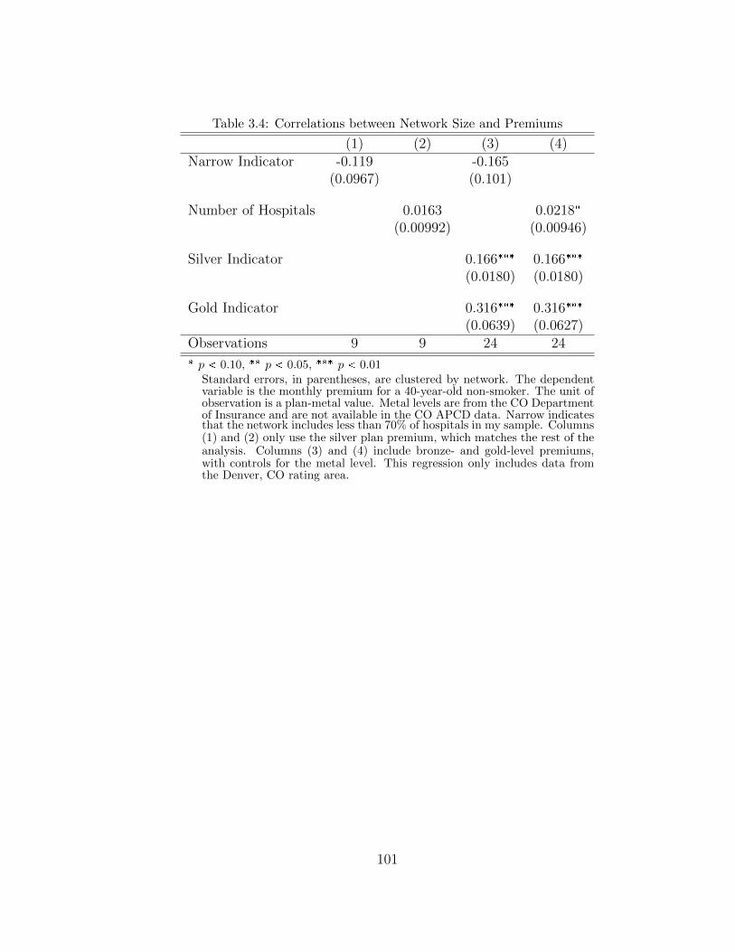
Table 3.4: Correlations between Network Size and Premiums
(1) (2) (3) (4)Narrow Indicator -0.119 -0.165
(0.0967) (0.101)
Number of Hospitals 0.0163 0.0218�
(0.00992) (0.00946)
Silver Indicator 0.166��� 0.166���
(0.0180) (0.0180)
Gold Indicator 0.316��� 0.316���
(0.0639) (0.0627)Observations 9 9 24 24� p 0.10, �� p 0.05, ��� p 0.01
Standard errors, in parentheses, are clustered by network. The dependentvariable is the monthly premium for a 40-year-old non-smoker. The unit ofobservation is a plan-metal value. Metal levels are from the CO Departmentof Insurance and are not available in the CO APCD data. Narrow indicatesthat the network includes less than 70% of hospitals in my sample. Columns(1) and (2) only use the silver plan premium, which matches the rest of theanalysis. Columns (3) and (4) include bronze- and gold-level premiums,with controls for the metal level. This regression only includes data fromthe Denver, CO rating area.
101

Table 3.5: Demand for Hospitals
Distance (Miles) �0.142��� �0.144���
(0.00196) (0.00200)
Disease-Hospital FE Yes YesAge-Hospital FE No Yes
Mean Elasticity �1.453 �1.479Std Dev Elasticity 0.922 0.938Observations 14441 14441
Standard errors in parentheses� p 0.10, �� p 0.05, ��� p 0.01
Standard errors are in parentheses. The unit of ob-servation is a county-disease-age-sex-hospital. Thedependent variable is the difference in the log mar-ket share of each hospital and the log market shareof the outside option. Both columns include disease-hospital fixed effects. Column (2) includes age-hospital fixed effects.
102

Table 3.6: Prevalence of Condition Categories
meanCertain Conditions Originating in the Perinatal Period 0.01Complications from Pregnancy, Childbirth and the Puerperium 0.29Congenital Anomalies 0.05Diseases of Genitourinary System 0.88Diseases of the Blood and Blood-forming Organs 0.10Diseases of the Circulatory System 0.49Diseases of the Digestive System 0.69Diseases of the Musculoskeletal System 1.36Diseases of the Nervous System 0.63Diseases of the Respiratory System 0.38Diseases of the Skin and Subcutaneous Tissue 0.16Endocrine, Nutritional and Metabolic Diseases 0.34Infectious and Parasitic Diseases 0.13Injury and Poisoning 2.25Mental Illness 0.15Neoplasms 1.00Residual Codes, Unclassified 2.93Symptions, Signs and Other Ill-defined Conditions 1.07
Conditions are defined as CCS codes. Prevalence is the number of visits per enrollee.Numbers are percentages.
Table 3.7: Prevalenceof Conditions by Age
meanAge 0-18 2.67Age 19-25 7.62Age 26-35 11.18Age 36-45 14.58Age 46-55 16.87Age 56-65 21.50Total 12.40
This table displaysthe average numberof visits per enrolleein each age group.Numbers are per-centages.
103

Table 3.8: Summary Statistics for WTP for Networks
Both Narrow Broadmean sd mean sd mean sd
All Enrollees 0.16 0.10 0.11 0.06 0.21 0.11Age 0-18 0.02 0.01 0.01 0.00 0.02 0.00Age 19-25 0.11 0.05 0.08 0.03 0.14 0.04Age 26-35 0.16 0.05 0.11 0.03 0.21 0.03Age 36-45 0.22 0.07 0.16 0.04 0.29 0.03Age 46-55 0.22 0.07 0.16 0.04 0.29 0.03Age 56-65 0.22 0.08 0.16 0.04 0.30 0.04Observations 19440 10800 8640
The unit of observation is age-gender-county-network. Summarystatistics are unweighted means, standard deviations of WTPmeasure.
Table 3.9: Demand for Networks
Value of Network 0.248��� 0.555���
(0.0353) (0.0469)
Fixed Effect Network County-Network
Mean Elasticity 0.0893 0.200Std Dev Elasticity 0.0652 0.146Observations 131980 131980
Standard errors in parentheses� p 0.10, �� p 0.05, ��� p 0.01
The unit of observation is age-gender-county-network. Depen-dent variable is the log of aggregate market share minus log ofnumber uninsured. OLS regression includes county and networkfixed effects.
104

Table 3.10: Premium Sensitivity
Network Id Narrow Ind α1r Mean Elasticity1 0 -0.00032 -1.882 0 -0.00028 -1.703 0 -0.00038 -2.124 0 -0.00033 -1.925 1 -0.00027 -1.786 1 -0.00062 -2.767 1 -0.00086 -2.978 1 -0.00029 -1.859 1 -0.00043 -1.93
The unit of observation is age-gender-county-network. Planspecific premium sensitivities are determined using first-ordercondition for optimal premium setting, then solving for α1rthe premium-sensitivity parameter. Observed premiums andprices are used. Estimated, rather than observed, hospital andplan market shares are used. First four rows correspond tobroad-network plans, last five narrow-network plans. Elastici-ties vary by age-gender-county because the market shares vary,elasticity column presents the unweighted mean across eachtype.
Table 3.11: Hospital-Specific Bargaining Parameters, ρHj
Hospital Id Endogenous Exclusion Exogenous Exclusion1 0.93 0.872 0.84 0.733 0.60 0.444 0.84 0.715 0.83 0.706 0.50 0.357 0.62 0.458 0.58 0.429 0.61 0.4910 0.68 0.5111 0.49 0.3012 0.66 0.5013 0.22 0.1614 0.65 0.48
The second and third columns are hospital-specific generic bargain-ing parameters, ρHj . Smaller values mean more bargaining power(smaller belief about subjective probability of breakdown). Inter-pretation depends on value relative to insurer bargaining parameter.This specification allows the θr to vary by insurer. The exogenousexclusion model sets P � 1.
105

Table 3.12: Insurer-Specific Bargaining Parameters, ρIr
Network Narrow P P � 1 P P � 1Id Ind. ρI ρI Split Split1 0 0.59 0.29 0.37 0.352 0 0.10 0.02 0.09 0.033 0 0.29 0.16 0.22 0.234 0 0.12 0.07 0.10 0.125 1 0.74 0.14 0.42 0.216 1 0.81 0.20 0.44 0.277 1 0.72 0.04 0.41 0.078 1 0.35 0.10 0.26 0.159 1 0.74 0.06 0.42 0.10
The third and fourth columns are insurer-specificgeneric bargaining parameters, ρIr . Smaller values meanmore bargaining power (smaller belief about subjectiveprobability of breakdown). This specification allows theθr to vary by insurer. The exogenous exclusion modelsets P � 1. The fifth and sixth columns display thesplit of surplus, given by Equation 3.7, with hospital 6to demonstrate how the parameters interact.
Table 3.13: Insurer-Specific ExclusionParameters θr
Network Id Parameter Estimate5 0.356 0.257 0.568 0.679 0.57
Larger values correspond to stronger(negative) relationship between num-ber of acceptable replacement hospi-tals and hospital’s share of surplus.0 would correspond to no correlation,while 1 would correspond to equiprob-ability of a deviating hospital beingpicked.
106

Table 3.14: Counterfactual Negotiated Prices
Type of Variation With Exclusion Nash-in-Nashθ � 1 1.56 0.62One θ 0.99 0.62θr by Ins. 1.27 0.62θj by Hosp. 1.20 0.62
This table reports the results of different counterfactual sim-ulations where exclusion is not allowed. Each row presentsa different set of θ parameters which capture the relation-ship between number of acceptable replacement hospitalsand hospital’s share of surplus. The first row assumes θ � 1which corresponds to assuming equiprobability of a deviat-ing hospital being picked. The second row allows for oneθ value. The third and fourth rows allow the θ to vary byinsurer and hospital, respectively. Breakdown has one hos-pital dropped from the network. The exogenous exclusionmodel sets P � 1.
107

4
Hospital-Insurer Bargaining in Selection Markets
4.1 Introduction
Hospitals are one of the most active industries for mergers and acquisitions. More
than 1700 hospitals were involved in acquisitions between 1994 and 2000 Cuellar
and Gertler (2003). At the same time, many local hospital markets have come to
be dominated by two to three large hospital systems (Moriya et al., 2010). Vogt
and Town (2006) argue that from 1990 to 2003 the HHI for the market increased by
fifty percent for typical person living in a metropolitan statistical area. A number
of studies argue that consolidation has led to large increases in hospital prices Vogt
and Town (2006). There has also been substantial concern about the impact of hos-
pital and physician consolidation on prices, quality and ultimately health insurance
premiums and coverage FTC (2004).
The concerns about premium growth is exacerbated by the Affordable Care Act
where much of the coverage is purchased in a marketplace setting, which, unlike
employer sponsored insurance requires consumers to pay most of the premiums. The
concern this paper raises is that rising premiums could lead relatively healthy con-
108

sumers to decide against purchasing insurance, raising premiums for other consumers.
Indeed, we argue standard merger analyses may understate the welfare loss due to
mergers in markets with adverse selection.
A typical merger analysis seeks to quantify the anti-competitive effects of a
merger. For example, do hospitals gain more bargaining power by merging? How-
ever, in a market with adverse selection, a merger may also effect welfare by changing
the pool of patients who are insured. We present a simple model with the following
intuition: if a merger leads to hospitals to negotiate higher prices, this may lead to
higher premiums, and the healthiest consumers being priced out of the market. This
may raise premiums even more. Therefore, a hospital merger may also have welfare
consequences through the channel of adverse selection. This has policy consequences
as our paper suggests anti-trust policy should be tighter in more adversely selected
markets.
Ultimately, the degree to which welfare loss is understated depends on how se-
lected the market is (i.e. are those that drop coverage much sicker or only somewhat
sicker than the pre-merger risk pool) and consumers’ premium sensitivities. The dif-
ficulty in assessing the welfare loss however is that price effects and selection occur in
different markets. In the upstream market hospitals set higher prices in their negoti-
ations with insurers. While adverse selection occurs in the downstream market where
insurers make decisions over what premiums to charge. We use the Nash-in-Nash
bargaining model, proposed by Horn and Wolinsky (1988) to specify a model which
takes into account the bilateral oligopoly structure of the market. This is similar to
Gowrisankaran et al. (2014) and Ho and Lee (2017). However, to our knowledge, this
is the first paper to account for the vertical structure of the industry while taking
adverse selection into account.
To compute the welfare effects, we estimate demand for hospitals and insurance,
similar to Capps et al. (2003). To incorporate selection we include measures of health
109
status in the previous year. We argue that due to the guaranteed issue regulations
in the Affordable Care Act that, while patients have private information about their
health status, insurers may not price on previous years’ health status, which is a
first order determinant of future costs. Therefore, our use of observed health status
captures much of the role of selection. This is a similar argument to Finkelstein and
Poterba (2014) which argues that selection can be estimated on observables which
are not used in pricing. We then estimate the Nash-in-Nash bargaining model using
these estimates of demand.
We show that without accounting for selection that star hospitals have under-
stated bargaining parameters, plans will offer those hospitals less if they drive sick
patients to their services, as in (Shepard, 2016). This is accounted for in the hospi-
tal bargaining parameter since the surplus function ignores the value. We then use
our estimates to simulate a merger, both using estimates which account for adverse
selection and estimates that do not.
4.2 Literature Review
This paper contributes to a growing literature on the role of market structure on
adverse selection. It is most closely related to Mahoney and Weyl (2016) who show
that a monopolist insurer exacerbates the welfare loss due to selection. Similar
to us, if a monopolist insurer charges supracompetitive premiums that may lead the
healthiest consumers to leave the market. Our paper incorporates a role for upstream
markups to also lead to supracompetitive premiums, through markups to hospitals
rather than insurers.
Our paper is also related to Cutler and Reber (1998), Bundorf et al. (2012),
Tebaldi (2016), and Lustig (2010) who empirically examine the role of adverse se-
lection and imperfect competition, though without necessarily examining how one
exacerbates the other. Shepard (2016) examines whether high cost hospitals lead to
110

selection.
This paper is also related to a growing literature on hospital-insurer bargaining.
Gowrisankaran et al. (2014) shows that a model of bargaining is necessary is simulat-
ing hospital mergers since assuming hospitals have price setting power would imply
hospitals have negative marginal costs when estimating hospital profit functions.
Our paper is more similar to Ho and Lee (2017) in that our empirical setting takes
place in a insurance marketplace rather than using the employer sponsored market.
Our paper builds on this literature by being the first to incorporate adverse selection
into a model of Nash-in-Nash hospital-insurer bargaining.
4.3 Theory
We demonstrate the intuition for the model by considering a competitive insurance
market with N consumers. We show that if there is adverse selection in the market
that this will exacerbate the welfare loss due to supracompetitive pricing. To clarify,
we define adverse selection as sicker patients being more likely to purchase insurance
or purchase more generous insurance. Let consumers vary by their expected medical
costs net of markup, ν, and an idiosyncratic value of insurance, ε. Let r be a
percentage markup for each unit of medical care changed by provider, so expected
medical costs are given by νi � r. I model linear utility functions, where we can think
of the utility functions as being an approximation to a model in which ν represents
the expected costs of a consumer and ε represents their degree of risk aversion. The
utility for consumer i when they have purchased insurance is given by:
U Ii � �premium� εi
When consumer i is uninsured, they are liable for their medical costs. And the
111
utility when they do not have insurance is given by:
UUi � �νi � r
A consumer signs up for insurance if their utility from being insured is greater
than being uninsured. Therefore demand is given by:
D �¸i
1p�premium� εi ¡ �νi � rq
We assume that ε � Unif r�.5, .5s. Premiums will be solved for in equilibrium
and markups and the distribution of ν will vary by case.
4.3.1 No Selection Case
We model there being no selection as having ν be constant. If ν is constant then
costs do not vary across consumers, so there is no selection (on costs). Because the
insurance market is assumed to be competitive, premium � ν � r. Therefore, due to
the linearity of the utility functions, D �°i 1pεi ¡ 0q � .5�N . Notice that this is true
regardless of the markup r. As markup increases, the cost of insurance increases in
turn, not affecting the insurance purchase decision. Welfare is not affected by hospital
markups in this simplified model because the quantity of insurance purchased does
not change. While this property represents a lower bound to the welfare loss due
to market power, it helps to clarify interaction between market power and selection.
Note that regardless of the markup the model is in the efficient equilibrium: all
consumers for which ε ¡ 0 purchase insurance.
4.3.2 Incorporating Adverse Selection
To incorporate adverse selection, suppose that ν � Unif r0, 1s. In this case consumers
with a large ν will be more likely to signup for insurance and will have higher costs,
leading to adverse selection. Figure 4.1 presents simulated results when r � 1,
112

that is there is no markup and r � 1.1, which would occur if upstream providers
negotiated a ten percent markup. The dashed lines represent average cost curves,
while the solid lines demand curves. The downward sloping cost curves represent
adverse selection, as the share of the population insured increases the average cost
of the insured population falls. The thick lines represent when there is a markup.
There are two different demand curves because as the markup rises the cost of being
uninsured rises shifting the demand (as a function of premiums) outward.
Figure 4.1: Demand and Average Cost Curve Under Adverse Selection
In the no markup case, premiums are .75 and the quantity insured is .28. When
there is an upstream markup of 10 percent, premiums rise to .85, a 13 percent in-
crease in premiums. This is driven by the fact that demand falls to .25, an eleven
percent drop in demand – which increases average costs. By simply assuming selec-
tion, quantity insured falls to .28 already well below the efficient level of insurance.
However, upstream markups exacerbate this because the quantity falls even further.
This highlights the interaction between upstream markups (which cause no drop in
quantity without selection) and selection, since quantity declines are larger when
upstream firms capture a markup.
113

4.4 Structural Model
While the previous section demonstrates that it is theoretically possible that a hos-
pital merger can exacerbate selection, the magnitude of this concern is an empirical
question. The impact of this interaction will depend on how much selection there
is, how much market power a hospital obtains in a merger, and the passthrough
rate of higher negotiated prices to consumers through higher premiums. To provide
empirical estimates for the magnitudes, we use the model of the hospital-insurance
market that follows Ho and Lee (2017). The notation and discussion will follow
Liebman (2017) (chapter 2 of this dissertation) closely, along with Shepard (2016)
who incorporates adverse selection into the Capps et al. (2003) insurance demand
model. We exploit the guaranteed issue and community rating features of the Af-
fordable Care Act that insurers cannot charge consumers different premiums based
on their health status. Therefore, we incorporate selection using consumers health
status in the previous year, which Finkelstein and Poterba (2014) refer to as “unused
observables.”
We model the hospital-insurer market in a similar way to Prager (2016), Ho and
Lee (2017), and Liebman (2017):
Stage 1: Prices and the network are negotiated between insurers and hospitals.
Stage 2: Insurers set their premiums.
Stage 3: Consumers choose which health plan to join.
Stage 4: Nature determines which consumers get sick.
Stage 5: Consumers who got sick choose which hospital to attend.
Stage 5 - Consumers who got sick choose which hospital to attend.
Consumer i, who lives in county m, is enrolled in health plan r, and gets sick with
condition d, has to choose a hospital in its health plan’s network. The utility of
114
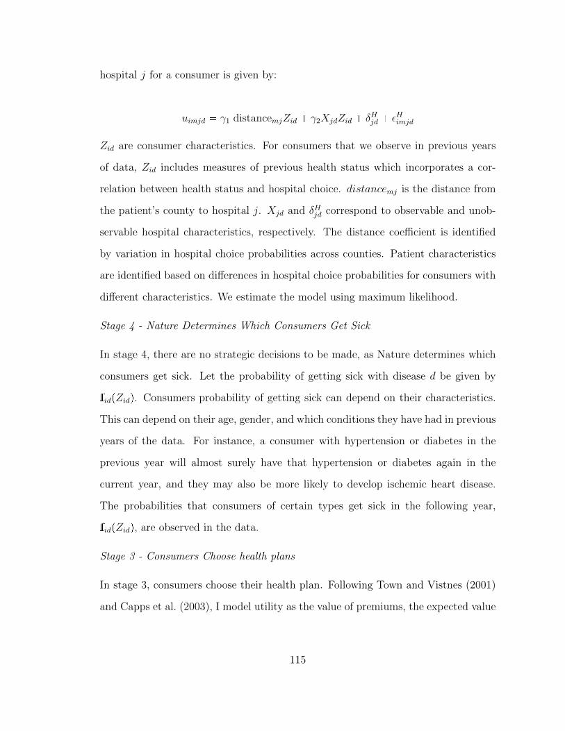
hospital j for a consumer is given by:
uimjd � γ1 distancemjZid � γ2XjdZid � δHjd � εHimjd
Zid are consumer characteristics. For consumers that we observe in previous years
of data, Zid includes measures of previous health status which incorporates a cor-
relation between health status and hospital choice. distancemj is the distance from
the patient’s county to hospital j. Xjd and δHjd correspond to observable and unob-
servable hospital characteristics, respectively. The distance coefficient is identified
by variation in hospital choice probabilities across counties. Patient characteristics
are identified based on differences in hospital choice probabilities for consumers with
different characteristics. We estimate the model using maximum likelihood.
Stage 4 - Nature Determines Which Consumers Get Sick
In stage 4, there are no strategic decisions to be made, as Nature determines which
consumers get sick. Let the probability of getting sick with disease d be given by
fidpZidq. Consumers probability of getting sick can depend on their characteristics.
This can depend on their age, gender, and which conditions they have had in previous
years of the data. For instance, a consumer with hypertension or diabetes in the
previous year will almost surely have that hypertension or diabetes again in the
current year, and they may also be more likely to develop ischemic heart disease.
The probabilities that consumers of certain types get sick in the following year,
fidpZidq, are observed in the data.
Stage 3 - Consumers Choose health plans
In stage 3, consumers choose their health plan. Following Town and Vistnes (2001)
and Capps et al. (2003), I model utility as the value of premiums, the expected value
115

of the network, and other plan characteristics:
Uimr � α1pZiq premiumir � α2 EpuimrpZiqq � ξmr � εPimr
premiumir is the premium that consumer i would face, which is, by law, constant
across counties within a rating area, except by age. Premium sensitivities are allowed
to vary by consumer characteristics, Zi. EpuimrpZiqq is the expected utility of the
providers in health plan r’s network. This is parameterized following the formulation
in Capps et al. (2003), which is the consumers option value of their hospital network,
accounting for probability that they get sick and need to choose a hospital. We
allow this value to depend on consumer observables, including past health status.
This captures that consumers who are more likely to get sick, or who prefer certain
hospitals may value having a broader network. We discuss the importance of having
past health status enter the model twice after discussing bargaining estimation.
Stage 2 - Insurers Choose Premiums
In stage 2, I assume that insurers engage in Nash-Bertrand competition over premi-
ums, given that their networks and marginal costs (which are the prices they pay
hospitals) are fixed.
Stage 1 - Providers and Insurers Bargain over Prices and the Network
We now specify the bargaining model. Let there by r � 1, ..., R insurers in a market
and j � 1, ..., N hospitals. Let there be s � 1, ...S hospital systems. A hospital
system will be denoted by S, where j P S if hospital j is a member of that hospital
system. I denote the set of hospitals in system s as Js. The Nash bargaining solution
between a hospital system and insurer is defined as the price which maximizes the
Nash product. Following Horn and Wolinsky (1988), the Nash product is defined as
the difference in profits for the insurer and the hospital system when the hospital
116

system is and is not included in the network. That is the surplus minus the surplus
in the case of disagreement. The insurers’ surplus for some network F is denoted by:
ΠIrpF , pq �
¸i
�premiumirpF , prq �
¸dPD
fidpZiq¸jPFr
pjdrpF ,Πrq � σimjdpFrq � other costsi
�
� SimrppremiumpF , pq, Fq
The insurers profit is given by the premiums they receive minus the costs they pay
out to hosptials to reimburse for the care of their patients. Each of the parameters
of the surplus function are observed or estimated in another stage of the model.
The Nash product is then defined as:
NPrs ��ΠIrpF , pq � ΠI
rpFzj P Ss, pq�brpsq � � ¸
jPJs
ΠHjrpF , pq
�bsprq
where ΠHjrpF , pq denotes the hospital’s profit function as a function of the network
and a vector of equilibrium prices. Following the notation of Gowrisankaran et al.
(2014), brpsq denotes insurer r’s bargaining weight with hospital system s and bsprq
denotes hospital system s’s bargaining weight with insurer r. Consistent with the
literature, we normalize bsprq � brpsq � 1, so these weights define how firms split
surplus between themselves.
Then the Nash bargaining solution is the vector of prices which maximizes the
Nash product:
p�rj � maxprj
NPrspprj|p��rjq
where p��rj is the equilibrium price vector for all other insurer-hospital pairs in the
market. We assume that if an insurance company and a hospital system disagree
that the entire system is dropped. Similar to Gowrisankaran et al. (2014), a hospital
merger will allow hospitals to negotiate higher prices since a disagreement would
117

mean that more hospitals are being dropped from the system. That is, the difference
between the insurers profit and disagreement value is larger.
As discussed during the stage of the model where consumers choose health plans,
observed characteristics enter in two locations in this specification. First, healthier
consumers may be less premium sensitive. Second, healthier consumers may value
networks less. If healthier consumers are less premium sensitive then healthier con-
sumers will sort into cheaper plans, regardless of their valuations for the services
provided. If hospitals merge, this would lead to higher markups and lead to the
healthiest consumers to shift across plans, regardless of whether the generosity of
the plans change. On the other hand if the services change, for example if a new
hospital is acquired by a system and therefore added to a network, then consumers
who value that hospital may join the plan, also potentially worsening the risk pool
for the insurer. Both of these mechanisms lead to more selection after a merger, and
potentially higher premiums for consumers as the healthiest consumers sort towards
less generous plans or drop out of the insurance market.
4.5 Conclusion
In this paper, we highlight how any increase in costs to an insurer may worsen
selection. Due to the prevalence of hospital mergers, we focus on that mechanism
for increasing insurers costs. In doing so, we bring together a literature on selection
in competitive markets, which does not consider the role of hospital market power
and a literature on hospital-insurer bargaining, which does not account for selection.
We show that theoretically hospital mergers exacerbate selection, and therefore the
welfare loss to a merger may be understated if selection is not accounted for. Finally,
we present a structural model of the hospital-insurer market which accounts for
adverse selection, which will allow policymakers empirically examine the magnitudes
of the welfare loss due to selection compared to the welfare loss using the merger
118

simulation framework without accounting for selection.
119

Appendix A
Chapter 2 Appendix
The left panel is the unweighted distribution of the reimbursement level, and the right panel isthe unweighted distribution of reimbursement changes. Source: CMS Part B National Summary
120

Table A.2: OLS and IV Estimates of the Effect of MMS on Shortage Days
(1) (2) (3) (4) (5) (6)Off Patent -5.549 -6.965 -26.63 -25.34 -9.513 -9.717
(13.65) (13.88) (26.65) (26.62) (14.38) (14.33)
Year ¥ 2005 � MMS 74.58** 130.8*(35.12) (70.40)
Year ¥ 2005 � Log MMS 6.445* 9.090* 7.038*** 8.406***(3.493) (4.821) (2.090) (3.085)
Constant 17.62* 56.96** 27.60***(9.403) (23.81) (10.53)
Observations 3094 3094 1701 1701 2714 2714# Drugs 308 308 152 152 244 244R2 0.169 0.167 0.223 0.222 0.193 0.193Drug Fixed Effect Yes Yes Yes Yes Yes YesYear Fixed Effect Yes Yes Yes Yes Yes YesIV Regression No Yes No Yes No Yes* p 0.10, ** p 0.05, *** p 0.01
Standard errors, in parentheses, are clustered at the drug level. The dependent variable isshortage days in a year. Off patent is 15 years since earliest Orange Book approval. Columns(1) and (2) are the OLS and IV estimates using the IMS MMS in levels, rather than logs, as thetreatment variable, respectively. Columns (3) and (4) use log of MMS again, but only includedrugs whose median price is below the sample median drug price. Columns (5) and (6) onlyuse 2003 and 2004 to calculate the IMS MMS. Each regression contains molecule fixed effectsand indicator variables for each year from 2002 to 2012.
121
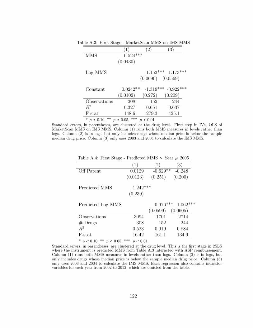
Table A.3: First Stage - MarketScan MMS on IMS MMS
(1) (2) (3)MMS 0.524***
(0.0430)
Log MMS 1.153*** 1.173***(0.0690) (0.0569)
Constant 0.0242** -1.319*** -0.922***(0.0102) (0.272) (0.209)
Observations 308 152 244R2 0.327 0.651 0.637F-stat 148.6 279.3 425.1* p 0.10, ** p 0.05, *** p 0.01
Standard errors, in parentheses, are clustered at the drug level. First step in IVs, OLS ofMarketScan MMS on IMS MMS. Column (1) runs both MMS measures in levels rather thanlogs. Column (2) is in logs, but only includes drugs whose median price is below the samplemedian drug price. Column (3) only uses 2003 and 2004 to calculate the IMS MMS.
Table A.4: First Stage - Predicted MMS � Year ¥ 2005
(1) (2) (3)Off Patent 0.0129 -0.629** -0.248
(0.0123) (0.251) (0.200)
Predicted MMS 1.242***(0.239)
Predicted Log MMS 0.976*** 1.062***(0.0599) (0.0605)
Observations 3094 1701 2714# Drugs 308 152 244R2 0.523 0.919 0.884F-stat 16.42 161.1 134.9* p 0.10, ** p 0.05, *** p 0.01
Standard errors, in parentheses, are clustered at the drug level. This is the first stage in 2SLSwhere the instrument is predicted MMS from Table A.3 interacted with ASP reimbursement.Column (1) runs both MMS measures in levels rather than logs. Column (2) is in logs, butonly includes drugs whose median price is below the sample median drug price. Column (3)only uses 2003 and 2004 to calculate the IMS MMS. Each regression also contains indicatorvariables for each year from 2002 to 2012, which are omitted from the table.
122

Appendix B
Chapter 3 Appendix
B.1 Data Appendix
Data on premiums and networks are collected from the CO Department of Insurance
website and insurance company websites. There are 12 companies in the market who
offer 22 different networks. The claims data always indicate the insurance company,
but only a few companies indicate which network the consumer has enrolled in. Of
these 12 companies, four companies in the data either did not submit their claims
or had too few enrollees for me to use their claims with any sort of precision. These
companies corresponded to six networks. Three other networks, while technically
offered in the Denver rating area were focused in other parts of the state and had
very little enrollment. For one company, I could not determine which of their claims
corresponded to the individual market. Finally, three companies offered a pair of
networks which I could not distinguish in the claims data. However, for only one
of the networks were the set of hospitals different. For these three pairs networks,
I treat the two networks as one, and for the one with different hospitals, I use the
smaller network to avoid characterizing out-of-network visits as in-network. This
123

leaves me with nine networks total, across seven companies. For simplicity, I treat
the two companies with observably different networks as different companies and use
the terms network, insurer and company interchangeably.1
The premium data are by company, network and metal level (metal levels: bronze,
silver, gold and platinum correspond to the actuarial value of the plans). In the claims
I do not observe the metal level, but the networks and negotiated prices do not vary
by metal level. Throughout the draft I use the cheapest silver plan offered for that
network as the premium.2
The sample of hospitals I use is the set of hospitals classified in the American
Hospital Association directory as General Medical/Surgical hospitals. This excludes
rehabilitation hospitals and children’s hospitals. I also exclude Veterans Affairs hos-
pitals. This leaves 17 hospitals and I drop two others since they have very few claims.
I match the hospitals using a fuzzy match by name, with the claims data, then hand
check them with their National Provider Identifier (NPI) in the national database of
providers.3
B.2 Complete Bargaining Model
In this section, I propose the complete version of my bargaining model. Compared
to the stylized version, I allow for many insurers and heterogeneity of surplus. The
discussion in this section closely follows the discussion of the stylized version, with
changes made as appropriate. This model is meant to provide foundations for the
empirical framework, so many of the assumptions were made with the five-stage
model in mind, however, I make a few modifications to keep this section self-contained
1 In future work, I plan to account for within company competition.
2 By law, plans are allowed to charge different premiums for each age group, but only up to athree-to-one ratio (that is, a plan may charge a 64-year-old only three times higher premiums thana 21-year-old). I adjust premiums for each age group accordingly, using a table from ... in theirinsurance filings.
3 https://npiregistry.cms.hhs.gov/
124

and highlight points which concern later stages of the game or estimation in footnotes.
B.2.1 Fundamentals
Consider a bargaining game between R insurers and N hospitals. Let R and N
denote the set of insurers and hospitals, respectively. At t � 0, each insurer r
publicly commits to Kr P N�, how many hospitals it would like to agree with, which
remains a fixed constant for the remainder of the game.4
Negotiations start at time period t � 1, step b.5 Let Frt and Art denote the sets
of hospitals who have and have not reached an agreement before period t. In each
period, every hospital j is either in Frt or Art for each insurer. That is, Frt and Art
are a partition of N for all t. At the beginning of each period, the set of hospitals
who will either make or receive an offer is chosen. I refer to this set of hospitals as
the “bargaining set,” denoted Krt. Either Nature or the insurer selects the set Krt
out of the set Art such that the number of hospitals selected, plus those who have
already reached an agreement, equal the number of hospitals the insurer would like
in the network, i.e., Kr � |Frt| � |Krt|. To simplify the model, I assume that Nature
will only choose hospitals that create enough surplus so that the hospital-insurer pair
could potentially reach an agreement.67
4 Commitment is a key assumption; without commitment the insurer would not exclude andwould lose the leverage gained from exclusion. In practice these contracts are renegotiated everyyear or every few years, and not all hospitals negotiate simultaneously. Furthermore, many ofthese insurance companies operate in many geographic markets, with different types of providers(hospitals, physicians, ambulatory care centers, etc.) and across many market segments (MedicareAdvantage, health exchanges, individual and employer insurance, etc.). Reneging in one marketcould make the exclusion threat less credible in others.
5 All periods after the first start with a step a.
6 Exclusion is exogenous when a hospital does not have enough surplus to reach an agreement.As Capps et al. (2003) point out, this will occur if added cost of a hospital (due to substitutiontowards that hospital and its marginal cost of treating patients) is higher than the marginal benefitof including that hospital.
7 Because I allow for externalities between hospitals, it is possible that if Nature is picking onehospital at a time then an earlier picked hospital may not provide enough surplus for the pair toreach an agreement. Instead, Nature determines all the sets of hospitals where each hospital could
125

Once the set Krt is specified, the game moves to the negotiation phase, step c,
of period t. When t is odd, the insurer makes offers to all hospitals in Krt simulta-
neously. When t is even, all hospitals in Krt make offers, denoted xjr, to the insurer
simultaneously. A player who receives an offer has a binary choice to either accept or
reject that offer. If the offer between hospital j and the insurer is accepted, hospital
j joins the set Frt�1 and remains in Fr for all subsequent periods. If an offer is
rejected at period t, that hospital joins the set Art�1. The game ends for insurer r
when Kr agreements have been made. Transfers are made at the end of the game.8
In order to have price determinacy, models of bargaining require a friction or cost
of negotiating. I include an exogenous probability of breakdown, similar to Binmore
et al. (1986). Starting in period t � 2 and in every following period, before Krt is
set, in step a, Nature determines whether a breakdown occurs. I allow hospitals and
insurers to have asymmetric beliefs about the subjective probability of breakdown
denoted by ρHj and ρIr, respectively.9 When a breakdown occurs, the game ends
and no further agreements can be made, though the surplus created and transfers
previously agreed to remain. All excluded hospitals, either due to the insurer reaching
Kr agreements or breakdown, receive zero surplus from that insurer. Renegotiation
of contracts is not allowed. The beliefs about the probability of breakdown are
assumed to be constant throughout time and do not vary based on which hospitals
have reached agreements. Players do not discount future surplus or transfers.
reach an agreement, then randomly chooses one of those sets.
8 For the purposes of the bargaining game, I assume that surplus is paid at the end of the period.In the full model, surplus is paid to the insurer (through premiums) in Stage 3, and the insurermakes transfers to hospitals in Stage 5. As I highlight later, players are negotiating over expectedsurplus in this stage.
9 Asymmetric beliefs are allowed for in Binmore et al. (1986), with the assumption of someappropriate behavioral model, for example heterogenous priors. I follow Binmore et al. (1986) anddo not specify this aspect of the model because it is not a key feature of the model. The main resultsof the model can be shown with symmetric beliefs. However, asymmetric beliefs help highlight theconcerns endogenous networks raise for the reduced-form analysis and are an important feature ofthe empirical model where the interpretation of this parameter is different.
126

For clarity, I respecify the timing of the model:
t=0. Each insurer r publicly commits to size of their network, Kr.
t � 1, 3, 5, ... (if |Fr| Kr agreements have been reached):
a. (Except period t � 1) Nature decides whether there is a breakdown.
b. Each insurer r picks which hospitals to make an offer to Kr.
c. Each insurer r makes simultaneous offers to the hospitals in Kr.
d. Hospitals in Kr simultaneously decide whether to accept or reject their of-
fer(s).
t � 2, 4, 6, ... (if |Fr| Kr agreements have been reached):
a. Nature decides whether there is a breakdown.
b. With equal probability Pp�q Nature chooses Kr � |Fr| hospitals to make an
offer Kr to each insurer r.
c. Hospitals in Kr make simultaneous offers to each insurer r.
d. Insurers simultaneously decide whether to accept or reject each offer.
The game stops when K hospitals have reached agreement or breakdown occurs.
Then payments are made.
I treat surplus as a primitive that takes as an input the network of hospitals and
transfers agreed upon by all hospital-insurer pairs and returns a dollar amount.10
That is, for any network Gr and set of transfers x, ΠrpG, xq is the total surplus
10 In the empirical section I specify the surplus function. I treat surplus as a primitive herebecause all of the inputs are determined at other stages of the game, conditional on the outcome ofthe bargaining game. Therefore, hospitals and insurers can determine the expected surplus valuesat any state of the world. Intuitively, this is the value of the expected premiums that the insurertakes as revenue, minus the expected sum of marginal costs of the services provided to all thehospitals in network.
127
generated. I omit the r subscript for G and the jr subscript for x because this
function depends on the networks of all insurers and transfers for all hospital-insurer
pairs. That surplus depends on the networks and transfers of all players allows for
flexibility in the externalities between hospitals and insurers. I include transfers
in this section because they affect the optimal premium setting for an insurer and
insurers compete over premiums. I assume that surplus is declining in transfers and
that adding any hospital to the network, holding transfers to all hospitals fixed, will
increase surplus.11 I assume all players are risk neutral.
The surplus functions allow for non-transferable utility because the surplus de-
pend on the transfers. Neither Binmore et al. (1986) nor Collard-Wexler et al. (2016)
allow for non-transferable utility, but Crawford and Yurukoglu (2012a) does. I do
not have an analytic solution with non-transferable utility, but can solve the model
numerically. For this section, I assume transferable utility, that is, hospital j’s ne-
gotiated transfer with insurer r does not affect the total surplus created by insurer
r’s network in its negotiations with hospital j. In practice if a hospital negotiates a
larger transfer, that may increase the insurer’s premiums, reducing the total surplus
available. This precludes a closed-form solution because larger transfers would re-
duce surplus, which would lower the agreed-upon transfer. This assumption is simply
expositional, in the empirical analysis, I use a fixed-point algorithm to solve for each
premium-transfer pair.
Throughout this section, I refer to surplus kept by insurers or hospitals and also
allow for these values to differ in the case of a breakdown.13 The term ΠIrpG, x,Kq
will represent the surplus insurer r captures, which is the total surplus, minus the
11 In the five-stage model, transfers effect surplus through premiums.12 Therefore, the sum ofexpected costs across all hospitals, not the transfer to any particular hospital, is the object ofinterest.
13 Again, these terms will all be explicitly specified in the empirical section, but for expositionalsimplicity these values are taken as primitives in the bargaining game.
128

markups to the hospitals. Likewise, ΠHjrpG, x,Kq represents the surplus hospital j
receives from patients enrolled in insurer r’s plan. Finally, I use ΠBr pG, x,Kq and
ΠIBr pG, x,Kq to denote the total surplus created and the surplus kept by insurer r
during a breakdown, respectively.
I assume an equilibrium exists and that all players know which equilibrium will
be played. I assume that players know the surplus functions, Π, and beliefs about the
probability of breakdown, ρ, for all the players. Throughout the bargaining stage,
insurers do not know the outcomes of decisions that other insurers make (including
the size of the networks, K, the bargaining sets, K, the set of agreements reached,
F , or transfers, x).14 That is, insurers do not update their information about other
insurers once decisions are made.
During negotiations, hospitals know the size of the network, K, the bargaining
set, K, and any agreements that have been made, F . Hospitals never learn the
transfers other hospitals are offered, offer, or agree to throughout the game.15 To
rule out informational asymmetries, I assume that the hospitals do not use their
information with one insurer when negotiating with a different insurer. Likewise, I
do not allow insurers to use information about their negotiations with other hospitals.
To give an example of these informational assumptions, consider a multilateral
negotiation where each hospital sends a delegate to negotiate with a delegate from
each insurer. Each insurer is located in a separate building, so delegates from dif-
ferent insurers cannot communicate, nor can delegates from one hospital negotiating
with different insurers. Once in the building, there is a waiting room where the in-
14 For the purposes of the bargaining game, I assumed that surplus was paid at the end of theperiod. Information about other insurer’s networks and premiums are not known until after Stage2, when premiums are set. These informational assumptions may be realistic if insurers do notreveal information about their networks to others prior to selling their products. My empiricalsetting is the first year of the exchange marketplace, which may restrict insurers’ ability to look atthe networks in the previous year. Information about other insurers’ prices are proprietary.
15 Other hospital’s negotiated prices are proprietary.
129
surer announces the size of the network, Kr.16 Then, the insurer lists all the hospital
delegates who will be called to negotiate, so all the delegates at that building know
which hospital delegates were included in the bargaining set. Then all the hospital
delegates in the bargaining set go into separate offices, each with a separate insurer
delegate. Offers are made without any communication outside of the pair of dele-
gates negotiating. Finally, after offers are accepted or rejected in that period, which
agreements are made is announced to all the delegates at that building.
While the model in this section allows for a much richer and more realistic empir-
ical framework, the drawback is that it increases the number of strategies available
and the number of resulting equilibria. This requires strong assumptions to regain
tractability. However, even if this was a less restrictive framework, I do not have
data on whether other strategies are used in practice, and if they are, they will be
accounted for in the bargaining parameters of the empirical model. While these
are strong restrictions on the model, this is a critique of the Nash-in-Nash model
generally. One interpretation of my paper is as a constructive criticism of these
restrictions: I am allowing for an additional strategy (the threat of exclusion) for
which data are available and demonstrating how to incorporate it into the tractable
and rich empirical framework the Nash-in-Nash model provides.
B.2.2 Equilibrium Strategy Profile
In this subsection, I propose a strategy profile which is a Markov-perfect equilib-
rium (MPE). The concept of an MPE restricts the set of equilibria to the subset of
subgame-perfect Nash equilibria for which the only aspect of the history that influ-
ences strategies is the current state. In particular, this implies that if negotiations
happen at t� 1, the probability of any hospital in Art�1 to be chosen to bargain at
t� 1 is independent of the identity of hospitals which rejected an offer at t.
16 The hospital delegates in the waiting room are Art.
130
In period t � 0, each insurer chooses its profit-maximizing size of the network,
given its expectation about the network sizes of other insurers. Let ΠIrpKr;K�rq
be the surplus the insurer receives in equilibrium when choosing network size Kr,
given that they expect other insurers to choose size K�r. In equilibrium each insurer
chooses Kr such that ΠIrpKr;K�rq ¥ ΠI
rpK1r;K�rq for all K 1
r ¤ N .
In odd periods t � 1, ...,8, step b, the insurer picks a bargaining set Krt such that
|Krt|�|Frt| � Kr. When making this choice, the insurer chooses its profit-maximizing
network. Let ΠIrpGrt,G�rt, x,Kq denote the expected surplus to the insurer given
the equilibrium outcomes when insurer r chooses network Grt and expects all other
insurers to choose the networks G�r and transfers x at t. Then the insurer chooses
the network Grt such that ΠIrpGrt,G�r, x,Kq ¥ ΠIpG 1rt,G�r, x,Kq for all G 1rt such that
|G 1rt| � Kr and Frt � Grt.17
Let Vjrt�1pFrt�1,F�r, x,Kq and Wrt�1pFrt�1,F�r, x,Kq denote hospital j’s and
insurer r’s expected value of having not reached an agreement before the beginning
of period t � 1, conditional on expectations about future agreements with insurer
r, Frt�1, networks formed by other insurers, F�r, and expectations about others’
transfers x.18 Given that players know the bargaining set when making or receiving
an offer, players can determine which hospitals will have reached agreements before
receiving their offers in period t. Therefore, in negotiations with hospital j, the
continuation value to the hospital and insurer during the offer stage of period t is
Vjrt�1pFrt�1ztju,F�r, x,Kq and Wrt�1pFrt�1ztju,F�r, x,Kq, where Frt�1 takes into
account those who have already reached an agreement (Frt�1) and those who are
expected to reach an agreement (some subset of Krt). This excludes hospital j
because the negotiation including hospital j is the one where a deviation is being
17 The condition Frt � Grt simply means that they are choosing the entire network, conditional onFrt having already agreed.
18 Because Art�1 and Frt�1 partition N , it is sufficient to just use Frt�1 as the state space.
131
considered. Because I use the MPE solution concept, the time period does not affect
the value functions, except for whether the state is even or odd. However, I use t
subscripts to clarify timing. In periods, t � 1, ...,8, step c, the players which make
offers propose their counterpart’s continuation value. The player who is offered their
continuation value will accept.
I assume that in equilibrium there will be immediate agreement:19
Assumption ImmAgg (Immediate Agreement). Suppose the value of the primitives
is such that a possible equilibrium involves immediate agreement (Kr agreements are
reached in period t � 1 for each r) and that this equilibrium is played.
In the simplified model there are two reasons why it is unprofitable for the insurer
to delay. First, the expected costs of breakdown are higher if fewer hospitals have
agreed at any point in time. Second, at least in the stylized model delay improves
the continuation value of a hospital who reaches an agreement at t � 1 because the
probability they are picked again if they deviate is higher than when all hospitals
agree at period t � 1. This is a similar argument to Moller (2007) who argues that
when the timing of agreements is endogenous, there is an incentive for simultaneous
agreements when the externalities between players weakens over time. Finally, In
the more general model, the insurer may also be left with a less profitable network
if they allow Nature to choose which hospitals remain.
B.2.3 Determining Continuation Values
Now, I discuss the equilibrium outcomes and compute the continuation values, given
the strategies specified in the previous section. While all hospitals agree in the
19 Without Assumption A.ImmAgg, the model is not fully specified. In particular, expectationsabout the network in future periods and whether there is enough surplus available to reach agree-ments need to be considered. Expectations no longer matter because the case where the deviatinghospital is chosen is the only relevant case. Assuming immediate agreement also assumes that eachhospital in the network provides enough surplus to be included.
132

first period, continuation values depend on the expected value for hospital j after
deviating from the equilibrium and rejecting the offer. Consider hospital j’s decision
to deviate from the equilibrium and reject the offer (in period t � 1 only). Deviating
hospital j’s expected value for period t � 2, given equilibrium strategies, simplifies
to:
Vjrt�2pKr1ztjuq � ρHj � 0 (B.1)
�
��ΠrpKr1, xpKr1qq �
¸iPpKr1ztjuq
ΠHirpKr1, xpKr1qq �Wt�3pKr1ztju, xpKr1qq
��
� p1 � ρHj q �Ppj P Kr2|Kr1ztjuq
where Ppj P Fr|Fr, Krq denotes the probability that hospital j is included in network
Fr, given that the hospitals in Fr have already reached an agreement and that Kr
hospitals will ultimately reach an agreement (barring a breakdown). I drop notation
for other networks (both F�r and K) because the player’s expectations about these
values are unchanging. With probability ρHj , breakdown occurs and the hospital gets
nothing. With probability p1�ρHj q, agreements are made possible in period t � 2. In
period t � 2, with probability Ppj P Kr2|Kr1ztjuq, hospital j will be chosen to make
an offer. The most the hospital can ask for is all the surplus the insurance company
receives, net of what it pays out to other hospitals and the insurer’s continuation
value. Because in equilibrium all hospitals reach an agreement at t � 1, in considering
the value of deviating, hospital j expects the payments to all other hospitals are
formed with the expectation that all hospitals in Kr1 will reach an agreement at
t � 1.
If hospital j were to deviate, then the network would consist of all the hospitals
in the original bargaining set except hospital j, i.e., Fr2 � Kr1ztju.20 Since I am
20 Since I am focusing on a hospital that deviated, by definition j P Kr1.
133

computing hospital j’s value of deviation, I focus on the case where it is picked in
the following period. Therefore, the input to Πrp�q is Kr1 because, conditional on
hospital j’s offer being accepted, the final state will be Kr1.21 Finally, the input to
Wrt�3p�q is Kr1ztju because if the offer is not accepted, then the state going into
period t � 3 will be Kr1ztju. However, all other transfers will have been agreed upon
under the expectation that Kr1 would have been the outcome of the negotiations in
t � 1. Notice that until the final agreement is made, the set of hospitals which will
have agreed at any given period remains unchanged at Kr1ztju.
Now, I solve for the insurer’s value function by considering the case where it
deviates at period t � 2. In this case, the insurer will pick the most profitable
network Kr1 again, so it chooses the same hospital j which deviated previously. The
insurer’s expected value in t � 3, given that the hospitals in Kr1ztju have agreed, is:
Wrt�3pKr1ztjuq (B.2)
� p1 � ρIrq
��ΠrpKr1, xpKr1qq �
¸iPpKr1ztjuq
ΠHirpKr1, xpKr1qq � Vjrt�4pKr1ztju, xpKr1qq
��
� ρIrΠIBr pKr1ztju, xpKr1qq
With probability p1 � ρIrq, the game goes forward and the insurer offers hospital
j its continuation value, keeping the remainder of the surplus that was not paid
out to other players. With probability ρIr, breakdown occurs and the insurer receives
ΠIBr pKr1ztju, xpKr1qq. Notice that transfers are determined based on the expectation
that Kr1 will have been formed, since these were the expectations of other hospitals
in Kr1, besides deviating hospital j.
21 Note that in this case all transfers would be the same as if it happened in period t � 1, sincethe other hospitals reached this agreement with an expectation that all hospitals would reach anagreement. The strategic situation is the same for hospital j as it was in period t � 1.
134
B.2.4 Bargaining Results
To calculate transfers, I consider a unilateral deviation by each hospital j P Kr1
separately. Because of immediate agreement, a unilateral deviation would imply
there is only one additional agreement remaining. At this point the state of the
game does not change from period t � 2 until an agreement is reached (condi-
tional on the state being even or odd). Because the value functions only depend
on the state, and the state only depends on whether the time is even or odd,
Vjrt�2pKr1ztju, xpKr1qq � Vjrt�4pKr1ztju, xpKr1qq � ... � Vjr evenpKr1ztju, xpKr1qq
and likewise
Wrt�3pKr1ztju, xpKr1qq � Wrt�5pKr1ztju, xpKr1qq � ... � Wr oddpKr1ztju, xpKr1qq.
Therefore, for each insurer-hospital pair I have two unknowns (Vjr evenp�q andWr oddp�q)
and two equations linear in the unknowns, so there exists a unique solution that can
be represented with a closed form (conditional on Ppj P Kr2|Kr1ztjuq). Proposition
3 presents this solution:
Proposition 3. The equilibrium outcome of this game is given by:
xjrpKr1q �ΠMARGjr pKr1q � rPpj P Kr2|Kr1ztjuq � p1 � ρHj qs � pρ
Irq
1 � p1 � ρIrq � rp1 � ρHj q �Ppj P Kr2|Kr1ztjuqs
Where the marginal surplus is defined as:
ΠMARGjr pKr1q � ΠrpKr1, xpKr1qq �
¸iPpKr1ztjuq
ΠHirpKr1, xpKr1qq � ΠIB
r pKr1ztju, xpKr1qq
Note that marginal surplus is not a value that I am assuming, but rather this is a
derived value.
135
Relationship to Rubinstein Outcomes
My first result states that when Kr � N , meaning the insurer chooses not to exclude,
the model predicts N outcomes that match the outcomes in Rubinstein (1982). In
particular, Kr � N implies that Pp�q � 1, i.e., hospitals who reject an offer in the
previous period will be picked with probability one. The solution reduces to:
Corollary 4. When K � N and Pp�q � 1, the equilibrium outcome simplifies to:
xjrpN q �ΠMARGjr pN q � p1 � ρHj q � ρ
Ir
1 � p1 � ρHj q � p1 � ρIrq
Allowing for exclusion, the results are the same as the Rubinstein result, except
that the hospitals’ risk of breakdown parameters are multiplied by their probability
of being chosen, as highlighted by the brackets in Proposition 3. One way to inter-
pret this is that my result is distinguishing the risk of breakdown from the risk of
exclusion due to the narrow-network. This also demonstrates how my model nests
the Nash-in-Nash solution. When there is no exclusion (or the probability of being
picked after deviating equals 1), each negotiation becomes the outcome of a pairwise
Rubinstein bargain, conditional on all the other negotiations. Collard-Wexler et al.
(2016) provides sufficient conditions under which this limits to the Nash-in-Nash
solution, similar to how Binmore et al. (1986) demonstrates that Rubinstein (1982)
limits to the Nash solution. The remaining results show how my model extends the
Nash-in-Nash model.
Narrow Networks Negotiate Smaller Transfers
My next result shows that the model with exclusion can imply smaller transfers.
This will be true if the following assumptions hold:
Assumption SN (Smaller Network). For positive numbers l: Pp�;Kq ¤ Pp�;K � lq
136

Assumption SN (A.SN) states that the probability of a hospital being selected
in the following period is smaller compared to the case where the insurer chose a
smaller network size in period t � 0. In a setting where hospitals are all acceptable
and have equal probability of being chosen this is a natural property. A smaller
network, holding N constant, means more hospitals are excluded. Therefore, if a
hospital deviates, there are more available hospitals to fill their slot, so the deviating
hospital has a lower chance of being picked again.
As a counterexample, suppose there are four hospitals and one insurer. If the
network size is K � 2, then the following networks are chosen with equal probability
t1, 2u, t2, 3u, t2, 4u. If the network size is K � 3 then the following networks are cho-
sen with equal probability t1, 3, 4u, t1, 2, 3u, t1, 2, 4u. Consider hospital 2’s decision
to deviate when K � 2 and after t2, 3u has been offered. In this case, hospital 2
knows with probability 1 it will be selected to negotiate in the following period. Now,
suppose that K � 3 and t1, 2, 4u have been offered to. After deviating, hospital 2
has a one-half probability of being included in the following period.
Assumption CMS (Constant Marginal Surplus). For positive numbers l:
ΠMARGjr pK;Kq � ΠMARG
jr pK;K � lq
Assumption CMS (A.CMS) states that the marginal surplus generated by a hos-
pital is constant in the size of the network. While the functional form in the empirical
section will imply lower marginal surplus, A.CMS isolates the role of bargaining lever-
age from changing the amount of surplus to be split. Without accounting for the
changing probability of exclusion, lower marginal surplus would imply that insurers
with larger networks negotiate smaller transfers. I argue that this effect is offset
by the exclusion effect, which is why in the data insurers with larger networks are
observed paying larger transfers.
Proposition 5. Under assumptions A.SN and A.CMS, insurers with smaller net-
137

works negotiate smaller transfers.
This is a straightforward consequence of Proposition 3. Intuitively, the reason
this occurs is that by excluding, the insurer is increasing the probability the hospital
gets zero, which worsens the hospital’s continuation value. Why this worsens the
continuation value is clear from equation B.1, as the value function is multiplied by
Ppj P Kr2|Kr1ztjuq. If hospital j disagrees when many hospitals are excluded, the
probability it gets nothing p1�Ppj P Kr2|Kr1ztjuqq is large. When few hospitals are
excluded, the probability of getting nothing is smaller, so the value of deviating is
larger.
B.3 Defining Acceptable Replacement Hospitals
To determine the probability that hospital j is picked after deviating in period t � 1,
I calculate the number of otherwise excluded hospitals that provide enough surplus to
make agreement with the insurer feasible. I refer to these as “acceptable replacement”
hospitals. For hospitals not in Kr1, their continuation in even periods is zero: In
equilibrium they do not maximize the insurer’s profit, so they will not be picked
again in t � 3. Therefore, any surplus they can extract at period t � 2 from the
insurer would make them better off. This simplifies checking which hospitals are
acceptable because I only need to check whether:
ΠIrpFr Y tiuztju,F�r, ppFq, Kq ¡ p1 � ρIqΠI
rpF , p,Kq � ρIΠIBjr pF ,Frztju, ppFq, Kq
(B.3)
That is, hospital i is acceptable if they provide enough surplus such that the insurer
would be better off paying them their marginal cost, rather than offering nothing
and waiting until the following period, where with probability ρI the insurer receives
their breakdown value and with probability p1 � ρIq it matches with hospital j.22
22 That is the insurer decides whether to make an offer to hospital i or wait to match with hospitalj in the following period.
138
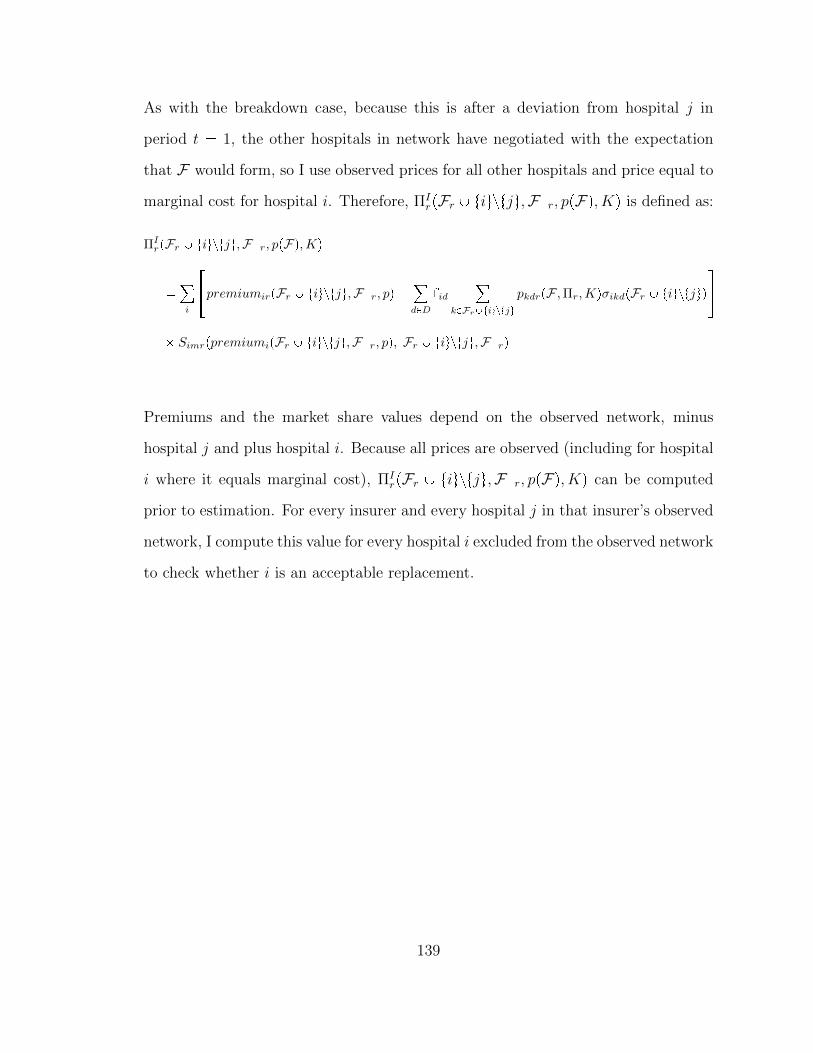
As with the breakdown case, because this is after a deviation from hospital j in
period t � 1, the other hospitals in network have negotiated with the expectation
that F would form, so I use observed prices for all other hospitals and price equal to
marginal cost for hospital i. Therefore, ΠIrpFr Y tiuztju,F�r, ppFq, Kq is defined as:
ΠIrpFr Y tiuztju,F�r, ppFq,Kq
�¸i
��premiumirpFr Y tiuztju,F�r, pq �
¸dPD
fid
¸kPFrYtiuztju
pkdrpF ,Πr,KqσikdpFr Y tiuztjuq
��
� SimrppremiumipFr Y tiuztju,F�r, pq, Fr Y tiuztju,F�rq
Premiums and the market share values depend on the observed network, minus
hospital j and plus hospital i. Because all prices are observed (including for hospital
i where it equals marginal cost), ΠIrpFr Y tiuztju,F�r, ppFq, Kq can be computed
prior to estimation. For every insurer and every hospital j in that insurer’s observed
network, I compute this value for every hospital i excluded from the observed network
to check whether i is an acceptable replacement.
139
Bibliography
(2004), “Improving Health Care: A Dose of Competition,” Tech. rep., Federal TradeCommission and U.S. Department of Justice.
Abaluck, J. and Gruber, J. (2011), “Choice Inconsistencies among the Elderly: Ev-idence from Plan Choice in the Medicare Part D Program,” American EconomicReview, 101, 1180–1210.
Abreu, D. and Manea, M. (2012), “Markov Equilibria in a Model of Bargaining inNetworks,” Games and Economic Behavior, 75, 1–16.
Academy of Managed Care Pharmacy (2013), “AMCP Guide to PharmaceuticalPayment Methods, 2013 Update,” Tech. rep.
Altman, D., Cutler, D., and Zeckhauser, R. (2003), “Enrollee Mix, Treatment In-tensity, and Cost in Competing Indemnity and HMO Plans,” Journal of HealthEconomics, 22, 23–45.
American Society of Anesthesiologists (2010), “The Anesthesia Perspective: TheImpact of Drug Shortages on Patients and Practitioners,” Presentation to FDA,September 27, 2010.
American Society of Clinical Oncology (2011), “Testimony of W. Charles Penley,MD,” Subcommittee on Health of the Committee on Energy and Commerce: Hear-ing Examining the Increase in Drug Shortages, September 23, 2011.
American Society of Hematology (2011), “Prescription Drug Shortages: Examininga Public Health Concern and Potential Solutions,” Testimony to Committee OnHealth, Education, Labor and Pensions, U.S. Senate, December 15, 2011.
Asker, J. (2016), “Diagnosing Foreclosure Due To Exclusive Dealing,” The Journalof Industrial Economics, pp. 375–410.
Baicker, K. and Levy, H. (2015), “How Narrow a Network Is Too Narrow?” JAMAInternal Medicine, 175.
Baicker, K., Mullainathan, S., and Schwartzstein, J. (2015), “Behavioral Hazard inHealth Insurance,” Quarterly Journal of Economics.
140
Bauman, N., Coe, E., Ogden, J., and Parikh, A. (2014), “Hospital networks: UpdatedNational View of Configurations on the Exchanges,” .
Beckert, W., Smith, H., and Takahashi, Y. (2015), “Competitive Price Discrimina-tion in a Spatially Differentiated Intermediate Goods Market,” pp. 1–42.
Berndt, E. R. (2002), “Pharmaceuticals in U.S. Health Care: Determinants of Quan-tity and Price,” The Journal of Economic Perspectives, 16, pp. 45–66.
Berndt, E. R. (2005), “Report of Independent Expert Prof. Ernest Berndt to JudgePatti B. Saris,” United States District Court of Massachusetts.
Berry, S. T. (1994), “Estimating Discrete-choice Models of Product Differentiation,”The RAND Journal of Economics, 25, 242–262.
Binmore, K., Rubinstein, A., and Wolinsky, A. (1986), “The Nash Bargaining Solu-tion in Economic Modelling,” The RAND Journal of Economics, 17, 176–189.
Borenstein, S., Bushnell, J. B., and Wolak, F. A. (2002), “Measuring Market Ineffi-ciencies in California’s Restructured Wholesale Electricity Market,” The AmericanEconomic Review, 92, pp. 1376–1405.
Bundorf, B. M. K., Levin, J., and Mahoney, N. (2012), “Pricing and Welfare inHealth Plan Choice,” 102, 3214–3248.
Burkett, J. (2014), “The Reality Behind Generic Drug Inflation,” Drug Options.
Camera, G. and Selcuk, C. (2010), “Multi-player Bargaining With Endogenous Ca-pacity,” Review of Economic Dynamics, 13, 637–653.
Capps, C., Dranove, D., and Satterthwaite, M. (2003), “Competition and MarketPower in Option Demand Markets.” The RAND Journal of Economics, 34, 737–763.
Carlton, D. W. (1978), “Market Behavior with Demand Uncertainty and Price In-flexibility,” The American Economic Review, 68, pp. 571–587.
Chipty, T. and Snyder, C. M. (1999), “The Role of Firm Size in Bilateral Bargaining:A Study of the Cable Television Industry,” Review of Economics and Statistics,81, 326–340.
Clemens, J. and Gottlieb, J. D. (2013), “In the Shadow of a Giant: Medicare’s Influ-ence on Private Payment Systems,” Working Paper No. 19503, National Bureauof Economic Resarch.
Collard-Wexler, A., Lee, R. S., and Gowrisankaran, G. (2016), “Bargaining in Bi-lateral Oligopoly: An Alternating Offers Representation of the “Nash-in-Nash”Solution,” .
141

Conti, R. M. and Berndt, E. R. (2013), “Anatomy of U.S. Cancer Drug Shortages:Technology, Market Structure and Price Competition,” NBER Working Paper.
Corlette, S., Volk, J., Berenson, R., and Feder, J. (2014), “Narrow Provider Networksin New Health Plans: Balancing Affordability with Access to Quality Care,” RobertWood Johnson Foundation.
Cramton, P. and Stoft, S. (2005), “A Capacity Market that Makes Sense,” ElectricityJournal 18, 43-54.
Crawford, G. S. and Yurukoglu, A. (2012a), “The Welfare Effects of Bundling inMultichannel Television Markets,” American Economic Review.
Crawford, G. S. and Yurukoglu, A. (2012b), “The Welfare Effects of Bundling inMultichannel Television Markets,” The American Economic Review, 102, 643–685.
Crawford, G. S., Lee, R., Whinston, M., and Yurukoglu, A. (2016), “The WelfareEffects of Vertical Integration in Multichannel Television Markets,” .
Cuellar, A. E. and Gertler, P. J. (2003), “Trends In Hospital Consolidation: TheFormation Of Local Systems,” 6, 77–87.
Cutler, D. M. and Reber, S. J. (1998), “Paying For Health Insurance: The Trade-off Between Competition and Adverse Selection,” The Quarterly Journal of Eco-nomics, 113, 433–466.
Cutler, D. M., Mcclellan, M., and Newhouse, J. P. (2000), “How Does Managed CareDo It?” The RAND Journal of Economics, 31, 526–548.
Dafny, L., Gruber, J., and Ody, C. (2015), “More Insurers Lower Premiums: Evi-dence from Initial Pricing in the Health Insurance Marketplaces,” American Jour-nal of Health Economics, 1, 53–81.
Dalton, C. M., Gowrisankaran, G., and Town, R. (2015), “Myopia and ComplexDynamic Incentives: Evidence from Medicare Part D,” .
Dana, James D., J. (2001), “Competition in Price and Availability When Availabilityis Unobservable,” The RAND Journal of Economics, 32, pp. 497–513.
Deneckere, R. and Peck, J. (1995), “Competition over Price and Service Rate WhenDemand is Stochastic: A Strategic Analysis,” The RAND Journal of Economics,26, pp. 148–162.
Dor, A., Grossman, M., and Koroukian, S. M. (2004), “Hospital Transaction Pricesand Managed-care Discounting for Selected Medical Technologies,” American Eco-nomic Review, 94, 352–356.
142

Duggan, M. and Scott Morton, F. M. (2010), “The Effect of Medicare Part D onPharmaceutical Prices and Utilization,” American Economic Review, 100, 590–607.
Dunn, A., Liebman, E., and Shapiro, A. H. (2014), “Developing a Framework forDecomposing Medical-Care Expenditure Growth: Exploring Issues of Representa-tiveness,” in Measuring Economic Sustainability and Progress, eds. D. W. Jorgen-son, J. S. Landefeld, and P. Schreyer, pp. 545–574, University of Chicago Press.
Elliott, M. and Nava, F. (2015), “Decentralized Bargaining: Efficiency and the Core,”.
Ericson, K. M. and Starc, A. (2015), “Measuring Consumer Valuation of LimitedProvider Networks ,” American Economic Review: Papers & Proceedings, 105,115–119.
Finkelstein, A. and Poterba, J. (2014), “Testing for Asymmetric Information Us-ing Unused Observables in Insurance Markets: Evidence from The U.K. AnnuityMarket,” Journal of Risk and Insurance, 81, 709–734.
Fox, E. R., Birt, A., James, K. B., Kokko, H., Salverson, S., and Soflin, D. L. (2009),“ASHP Guidelines on Managing Drug Product Shortages in Hospitals and HealthSystems,” American Journal of Health-System Pharmacy, 66, 1399–1406.
Fox, E. R., Sweet, B. V., and Jensen, V. (2014), “Drug Shortages: A Complex HealthCare Crisis,” Mayo Clinic Proceedings, 89, 361–73.
Gal-Or, E. (1997), “Exclusionary Equilibria in Health-Care Markets,” Journal ofEconomics and Management Strategy, 6, 5–43.
Gal-Or, E. (1999), “Mergers and Exclusionary Practices in Health Care Markets,”Journal of Economics and Management Strategy, 8, 315–350.
Ghili, S. (2016), “Network Formation and Bargaining in Vertical Markets: The Caseof Narrow Networks in Health Insurance,” .
Giovannelli, J., Lucia, K. W., and Corlette, S. (2015), “Realizing Health Reform’sPotential Implementing the Affordable Care Act: State Regulation of MarketplacePlan Provider Networks,” .
Gowrisankaran, B. G., Nevo, A., and Town, R. (2014), “Mergers When Prices AreNegotiated: Evidence from the Hospital Industry,” American Economic Review,105, 172–203.
Grabowski, H. G., Long, G., and Mortimer, R. (2014), “Recent Trends in Brand-Name and Generic Drug Competition,” Journal of Medical Economics, 17, 207–214.
143

Grennan, M. (2013a), “Price Discrimination and Bargaining: Empirical Evidencefrom Medical Devices,” The American Economic Review, 103, 145–177.
Grennan, M. (2013b), “Price Discrimination and Bargaining: Empirical Evidencefrom Medical Devices,” American Economic Review, 103, 145–177.
Gruber, J. and Mcknight, R. (2016), “Controlling Health Care Costs Through Lim-ited Network Insurance Plans: Evidence from Massachusetts State Employees,”American Economic Journal: Economic Policy, 8, 219–250.
Haeder, S. F., Weimer, D. L., and Mukamel, D. B. (2016), “Secret Shoppers FindAccess to Providers and Network Accuracy Lacking for Those in Marketplace andCommercial Plans,” Health Affairs, 35, 1160–1166.
Handel, B. R. (2013), “Adverse Selection and Regulation in Health Insurance Mar-kets: When Nudging Hurts,” American Economic Review, 103, 2643–2682.
Handel, B. R. and Kolstad, J. T. (2015), “Health Insurance for “Humans”: Informa-tion Frictions, Plan Choice, and Consumer Welfare,” American Economic Review,105, 2449–2500.
Handel, B. R., Koldstad, J. T., and Spinnewijn, J. (2015), “Information Frictions andAdverse Selection: Policy Interventions in Health Insurance Markets,” WorkingPaper.
Ho, K. (2009), “Insurer-Provider Networks in the Medical Care Market,” AmericanEconomic Review, 99, 393–430.
Ho, K. and Lee, R. S. (2015), “Insurer Competition in Health Care Markets,” Tech.rep., CEPR Discussion Papers.
Ho, K. and Lee, R. S. (2017), “Insurer Competition in Health Care Markets,” Econo-metrica.
Ho, K., Hogan, J., and Morton, F. S. (2015), “The Impact of Consumer Inattentionon Insurer Pricing in the Medicare Part D Program,” .
Horn, H. and Wolinsky, A. (1988), “Bilateral Monopolies and Incentives for Merger,”The RAND Journal of Economics, pp. 408–419.
Howard, D. (2014), “Adverse Effects of Prohibiting Narrow Provider Networks,” NewEngland Journal of Medicine.
Jackson, M. O. and Wolinsky, A. (1996), “A Strategic Model of Social and EconomicNetworks,” Journal of Economic Theory, 71, 44–74.
144

Jacobson, M., Earle, C. C., Price, M., and Newhouse, J. P. (2010), “How Medicare’sPayment Cuts For Cancer Chemotherapy Drugs Changed Patterns Of Treatment,”Health Affairs, 29, 1391–1399.
Kaakeh, R., Sweet, B. V., Reilly, C., Bush, C., DeLoach, S., Higgins, B., Clark,A. M., and Stevenson, J. (2011), “Impact of drug shortages on US health systems.”American Journal of Health-System Pharmacy, 68.
Kowalski, A. E. (2014), “The Early Impact of the Affordable Care Act, State byState,” Brookings Papers on Economic Activity.
Lafontaine, F. and Slade, M. (2008), “Exclusive Contracts and Vertical Restraints:Empirical Evidence and Public Policy,” in Handbook of Antitrust Economics, ed.P. Buccirossi, MIT Press.
Lee, R. S. (2013), “Vertical Integration and Exclusivity in Two-Sided Markets,” TheAmerican Economic Review, 103, 2960–3000.
Lee, R. S. and Fong, K. (2013), “Markov-Perfect Network Formation An AppliedFramework for Bilateral Oligopoly and Bargaining in Buyer-Seller Networks,” .
Lewis, M. S. and Pflum, K. E. (2015), “Diagnosing hospital system bargaining powerin managed care networks,” American Economic Journal: Economic Policy, 7,243–274.
Liebman, E. (2017), “Bargaining in Markets with Exclusion: An Analysis of HealthInsurance Networks,” pp. 1–61.
Liebman, E. and Panhans, M. (2016), “Hospital-Insurer Bargaining in Selection Mar-kets,” .
Lustig, J. (2010), “Measuring Welfare Losses from Adverse Selection and ImperfectCompetition in Privatized Medicare,” .
Magellan Rx Management (2013), “Medical Pharmacy Trend Report,” .
Mahoney, N. and Weyl, G. (2016), “Imperfect Competition in Selection Markets,”Review of Economics and Statistics.
Manea, M. (2015), “Models of Bilateral Trade in Networks,” in The Oxford Handbookon the Economics of Networks, eds. Y. Bramoulle, A. Galeotti, and B. Rogers,Oxford University Press.
Medicare Payment Advisory Commission (2003), “Report to Congress: Variationand Innovation in Medicare,” Chapter 9: Medicare Payments for Outpatient DrugsUnder Part B, June 2003.
145

Metzger, M. L., Billett, A., and Link, M. P. (2012), “The Impact of Drug Shortages onChildren with Cancer: The Example of Mechlorethamine,” New England Journalof Medicine, 367, 2461–2463.
Moller, M. (2007), “The Timing of Contracting With Externalities,” Journal of Eco-nomic Theory, 133, 484–503.
Moriya, A. S., Vogt, W. B., and Gaynor, M. (2010), “Hospital prices and marketstructure in the hospital and insurance industries.” Health economics, policy, andlaw, 5, 459–79.
Mullen, P. (2007), “The Arrival of Average Sales Price (ASP),” Biotechnology Health-care, June 2007.
Nash, J. (1950), “The Bargaining Problem,” Econometrica, 18, 155–162.
Office of Inspector General (2005), “Medicaid Drug Price Comparison: Average SalesPrice to Average Wholesale Price,” OEI-03-05-00200, June 2005.
Panel, A. E. (2009), “ASHP guidelines on managing drug product shortages in hos-pitals and health systems,” Am J Health-Syst Pharm, 66, 1399–406.
Panhans, M. (2016), “Adverse Selection in ACA Exchange Markets: Evidence fromColorado,” .
Prager, E. (2016), “Tiered Hospital Networks, Health Care Demand, and Prices,” .
Rey, P. and Tirole, J. (2007), “A Primer on Foreclosure,” in Handbook of IndustrialOrganization, vol. 3, pp. 2145–2220.
Ridley, D. B., Bei, X., and Liebman, E. (2016), “No Shot: Shortages in the UnitedStates Vaccine Market,” Health Affairs, 35.
Rosoff, P. M., Patel, K. R., Scates, A., Rhea, G., Bush, P. W., and Govert, J. A.(2012), “Coping with Critical Drug Shortages: An Ethical Approach for AllocatingScarce Resources in Hospitals,” Archives of Internal Medicine, 172, 1494–1499.
Rosse, J. (1970), “Estimating Cost Function Parameters Without Using Cost Data,”Econometrica, 38, 256–275.
Rubinstein, A. (1982), “Perfect Equilibrium in a Bargaining Model,” Econometrica,50, 97–109.
Sass, T. R. (2005), “The competitive effects of exclusive dealing: Evidence from theU.S. beer industry,” International Journal of Industrial Organization, 23, 203–225.
Scott Morton, F. M. (1999), “Entry Decisions in the Generic Pharmaceutical Indus-try,” The RAND Journal of Economics, 30, pp. 421–440.
146

Shepard, M. (2016), “Hospital Network Competition and Adverse Selection: Evi-dence from the Massachusetts Health Insurance Exchange,” .
Soares, I. G. (2016), “Mergers under Exclusive Dealing : An Empirical Analysis ofthe Fuel Industry,” pp. 1–45.
Stomberg, C. (2015), “Drug Pricing, Reimbursement, and Drug Shortages,” in Mea-suring and Modeling Health Care Costs, eds. A. Aizcorbe, C. Baker, E. R. Berndt,and D. Cutler, University of Chicago Press.
Tebaldi, P. (2016), “Estimating Equilibrium in Health Insurance Exchanges: PriceCompetition and Subsidy Design under the ACA,” .
Town, R. and Vistnes, G. (2001), “Hospital competition in HMO networks,” Journalof Health Economics, 20, 733–753.
U.S. Department of Health and Human Services (2011), “Economic Analysis of theCauses of Drug Shortages,” Assistant Secretary for Planning and Evaluation, Oc-tober 2011.
U.S. Department of Health and Human Services (2013), “Justification of Estimatesfor Appropriations Committees. Fiscal Year 2014,” .
Vogt, W. B. and Town, R. J. (2006), “How Has Hospital Consolidation Affected thePrice and Quality of Hospital Care?” .
Whinston, M. D. (2008), Lectures on Antitrust Economics, The MIT Press.
Woodcock, J. and Wosinska, M. (2012), “Economic and Technological Drivers ofGeneric Sterile Injectable Drug Shortages,” Clinical Pharmacology and Therapeu-tics, 93, 170–176.
Wooldridge, J. M. (2010), Econometric Analysis of Cross Section and Panel Data,MIT press.
Wu, V. Y. (2009), “Managed Care’s Price Bargaining with Hospitals,” Journal ofHealth Economics, 28, 350–360.
147

Biography
Eli Sellinger-Liebman was born June 23, 1989 in Berkeley, CA. He graduated magna
cum laude from American University in 2010 with a B.A. in Political Science with
a second major in Economics and a minor in Mathematics. He then worked at the
Bureau of Economic Analysis from 2010 to 2012 before starting his Ph.D at Duke
University in 2012. He earned his M.A. at Duke in 2014. He earned a Ph.D. in
Economics from Duke University in May 2017. He will be joining the faculty of the
University of Georgia in the Fall of 2017.
148