Essays on the Profitability of Winter Farming Enterprises

Essays on the Profitability of Winter Farming Enterprises

by

Manik Anand

A dissertation submitted to the Graduate Faculty of

Auburn University

in partial fulfillment of the

requirements for the degree of

Doctor of Philosophy

Auburn, Alabama

December 13, 2010

Copyright 2010 by Manik Anand

Approved by

Patricia A. Duffy, Co-chair, Professor of Agricultural Economics

Jason S. Bergtold, Co-chair, Affiliate Assistant Professor of Agricultural Economics

Diane Hite, Professor of Agricultural Economics

Randy L. Raper, Agricultural Engineer, USDA

Marshall C. Lamb, Supervisory Research Food Technologist, USDA

ii

Abstract

Cover crops can boost soil productivity as they increase soil organic carbon levels,

improve water infiltration and reduce soil erosion. In addition to the agronomic and

environmental benefits, they can also provide additional revenue-generating opportunities for

farmers such as winter annual grazing or selling of cover crop residues as a biofuel feedstock.

The objectives of this dissertation are to study various factors affecting these revenue generating

opportunities. The market for biofuel feedstock is not fully developed. Chapter 1 studies

farmers‟ willingness to adopt this practice and develops an estimate of the price at which they are

willing to sell the cover crop residues. Chapter 2 focuses on the agronomic and environmental

aspects of biomass removal and the profitability of selling crop residues as a biofuel feedstock.

Chapter 3 looks at winter annual grazing as an alternative revenue generating option provided by

cover crops. It compares the risks and returns for a cattle owner who has the option of placing

the cattle in a pasture before sending them to feedlot or to skip the pasture and send the cattle

directly to the feedlot.

iii

Acknowledgments

I dedicate this dissertation to my parents, especially my father Dr. Ram Rattan Anand and

my father-in-law Daulat Ram Saini. It‟s with their encouragement and blessings, I have been

able to reach this level.

I express my sincere gratitude to my co-chairs Dr. Jason S. Bergtold and Dr. Patricia A. Duffy

for their support and guidance. I would like to thank my committee members Dr. Diane Hite, Dr.

Randy L. Raper and Dr. Marshall Lamb for their guidance. I would like to extend my

appreciation to all the people at the USDA-ARS National Soils Dynamics Lab, Auburn, Aabama

for providing me the necessary support, infrastructure and financial assistance. I am also thankful

to all the faculty members, staff and fellow students at Department of Agricultural Economics

and Rural Sociology for their support throughout my doctoral studies. I am also thankful to Dr.

David Archer and Elizabeth Canales for their inputs in chapter 2.

Finally, I would like to acknowledge the never ending love and support that my wife

Monika and my lovely daughter Siya provided me.

iv

Table of Contents

Abstract………………………………………………………………………………………….ii

Acknowledgments........................................................................................................................ iii

List of Tables ............................................................................................................................... vi

List of Figures ............................................................................................................................ viii

Chapter 1: Farmers‟ Willingness to Produce Cellulosic Biofuel Feedstocks: Examining the

Case for Cover Crops in the Southeast .......................................................................... 1

Introduction ..................................................................................................................... 1

Cover Crops for Conservation and Biofuel Purposes ..................................................... 4

Data ................................................................................................................................. 7

Conceptual Framework ................................................................................................... 9

Results and Discussion ................................................................................................. 13

Conclusions ................................................................................................................... 18

References ..................................................................................................................... 20

Chapter 2: Balancing Feedstock Economics and Ecosystem Services ...................................... 46

Introduction ................................................................................................................... 46

Literature Review .......................................................................................................... 48

Case Study .................................................................................................................... 53

Challenges and Opportunities ....................................................................................... 64

Conclusions ................................................................................................................... 68

References ..................................................................................................................... 69

v

Chapter 3: Risks and Returns for Cattle Owners under Contract Grazing ................................. 95

Introduction ................................................................................................................... 95

Data ............................................................................................................................... 97

Model .......................................................................................................................... 100

Results ......................................................................................................................... 103

Conclusions ................................................................................................................. 106

References ................................................................................................................... 107

vi

List of Tables

Table 1.1: Summary Statistics for Survey Respondents and Sample Population ....................... 29

Table 1.2: Variable Description for Cover Crop Adoption Model ............................................. 30

Table 1.3: Estimation Results for the Selection PROBIT Model ............................................... 32

Table 1.4: Estimation Results of the Elicitation (WTA MBDC) Model .................................... 34

Table 2.1: Reported effects of Biomass Harvesting and/or Removal in the Literature for

Alternative Biofuel Feedstock Sources ...................................................................... 84

Table 2.2: Farm Optimization Model ......................................................................................... 85

Table 2.3: Response Functions for Soil Organic Carbon (SOC), Soybean, Corn and Nitrogen

for All Four Tillage Practices .................................................................................... 87

Table 2.4: Average Crop Yields at Swan Lake Research Farm near Morris, MN. 1997-2003 .. 88

Table 2.5: Cash Crop Cost Budgets for Corn and Soybean, 2008 ($/ acre) ............................... 89

Table 2.6: Biomass Costs for Corn Stover Removal .................................................................. 90

Table 2.7: Comparison of Farm Profits under Different Tillage Practices ................................. 91

Table 3.1: Experiment Details for Pasture Data (E V Smith Research Center, Shorter, AL) .. 109

Table 3.2: Summary Statistics for Pasture Data (E V Smith Research Center, Shorter, AL)

(2006-2009).............................................................................................................. 110

Table 3.3: Summary Statistics for Feedlot Data (Decatur County Feed Yard, Oberlin, KS)

(2006-2008) ............................................................................................................. 111

Table 3.4: Regression Results for the Weight Gained at the Pasture ....................................... 112

Table 3.5: Regression Results for the Weight Gained at the Feedlot ....................................... 113

Table 3.6: Returns on Investment (ROI) for 100 Cattle under Different Starting Weights

and Different Feeding Options................................................................................. 114

vii

Table 3.7: Estimates of First and Second Degree Stochastic Dominance ................................ 115

viii

List of Figures

Figure 1.1: Selection and Elicitation (MBDC) Question from Survey ....................................... 36

Figure 2.1: Change in Farm Profits with Change in Biomass Prices ......................................... 92

Figure 2.2: Change in Farm Profits with Change in Carbon Prices ........................................... 93

Figure 2.3: Response Surface of Farm Profit versus Biomass Price Showing Removal Rate

Contours for a Case Farm Responsible for Harvesting of the Biomass .................. 94

Figure 3.1: Stoplight Chart Comparing Return on Investments under Different Starting

Weights and Feeding Options ................................................................................ 116

Figure 3.2: Stoplight Chart Comparing Return on Investments under Different Contract

Pricing and Feeding Options .................................................................................. 117

Figure 3.3: Stochastic Efficiency with Respect to a Function (SERF) under a Negative

Exponential Utility Function.................................................................................. 118

1

Farmers’ Willingness to Produce Cellulosic Biofuel Feedstocks:

Examining the Case for Cover Crops in the Southeast.

I. INTRODUCTION

Production agriculture has the potential of providing a renewable energy source in

the form of cellulosic biofuel feedstocks for energy production (Rosillo-Calle et al., 2007).

Technological advances are shifting biofuel feedstock production in the U.S. from grains to

cellulosic sources. Carbon rich cellulosic materials can be obtained from a variety of sources

such as crop residues (e.g. corn stover and wheat straw), perennial crops (e.g. switchgrass) and

waste materials (e.g. forest residues) (Heid, 1984, Turnhollow, 1994). A potentially promising

cellulosic source in the Southeast is high-residue cover crops, which have the potential of

providing a sustainable biofuel feedstock source, while providing conservation benefits as well

(Raper et al., 2009).

Harvesting of cover crop residues as a cellulosic biofuel feedstock source may

provide an additional income stream for farmers in the Southeast. This area of the country is

particularly suited for growing both heavy residue winter and summer cover crops (Clark, 2007).

However, the decision to grow heavy residue cover crops as a biofuel feedstock may be

complicated by the reduction in conservation benefits resulting from biomass removal from the

soil surface. Leaving cover crop residues as mulch on the soil surface can provide both

2

agronomic and environmental benefits, such as increased soil organic matter, decreased soil

erosion, weed suppression and improved cash crop productivity (Snapp et al., 2005). Although

these benefits may not be assigned a direct monetary value, it is necessary to compare the

agronomic, economic and environmental benefits and costs, when considering growing a cover

crop as a cellulosic biofuel feedstock source (Wilhelm et al., 2004).

To further complicate the decision-making process for farmers, markets for

cellulosic biofuel feedstocks either do not exist or are still in the development stage. Prices for

many cellulosic feedstocks have not yet been discovered. Some studies have focused on the

economic, logistical and technical feasibility of producing alternative sources of biofuel

feedstocks sources. These studies have provided break-even prices for alternative cellulosic

sources that range between $30 to $45 per dry ton of cellulosic material (de La Torre Ugarte, et

al., 2007; Gallagher et al., 2003; Graham, 1994; Graham et al., 2007; Heid, 1984; Perlack et al.,

2005; Walsh et al., 2003). While break-even prices provide useful information, they do not take

into account farmers‟ reservation price or the premium needed to take account of things such as

foregone conservation benefits, risk aversion, uncertainty, and impacts on future cash crops.

In addition, a very limited amount of research, that too in the form of regional

studies, has been conducted to understand the socio-economic factors influencing the adoption of

alternative cellulosic sources and technologies (Bransby, 1998; Hipple and Duffy, 2002; Jensen

et al., 2007). Kelsey and Franke (2009) studied Oklahoma market and are of the opinion that a

major factor of non-adoptability to biofuel crops is lack of information. Producers desire more

information about biofuel crop production thus increasing farm profitability by growing biofuel

crops. Jensen et al., (2007) studied switch grass production in Tennessee as a bioenergy crop and

found out that only 21% farmers were aware of using switchgrass as a bioenergy crop. They were

also concerned that about the undeveloped market and need of technical assistance. Hipple and Duffy

3

(2002) reported that most Iowa farmers were cautious of making a commitment to grow switchgrass

before knowing the outcome.

These regional studies of biomass supply have tended to ignore the socio-

economic factors affecting farmers‟ willingness to produce alternative biofuel feedstock sources,

including the timing, location and extent of adoption (Rajagopal and Zilberman, 2007). Since

none of the studies have explored cover crop residues as an alternative, agricultural producers

and policymakers do not have an accurate reflection of the prices at which these feedstocks

would be available. This severely limits the decision-making ability of farmers in the Southeast,

an area which has the potential to provide a broader range of potential cellulosic feedstock

sources.

The purpose of this paper is to assess farmers‟ willingness to grow high residue

cover crops as a cellulosic biofuel feedstock. Both the potential socio-economic factors

influencing the adoption of such enterprises and price discovery for supplying cover crop

residues are explored. A survey was conducted to gather agronomic, economic and socio-

demographic information on farmers‟ cover crop decisions, as both a conservation practice and

potential biofuel feedstock. A two-step modeling approach, following a multiple bounded

contingent valuation methodology, was used to understand the agronomic, farm management and

demographic factors affecting farmers‟ willingness to produce and harvest cover crop biomass as

a biofuel feedstock source at different selling prices.

The remainder of the paper is organized as follows. Section two provides

background concerning the benefits and costs of adopting cover crops for both conservation and

biofuel purposes. This section examines some of the tradeoffs to be considered by farmers in

order to decide whether they are willing to grow cover crops as a biofuel feedstock or not. The

survey, data and explanatory variables used in the model are presented in section three. Section

4

four details the conceptual and modeling frameworks, which is followed by the presentation of

model results in section five. Section six provides concluding remarks and avenues for future

research.

II. COVER CROPS FOR CONSERVATION AND BIOFUEL PURPOSES

Cover crops can boost soil productivity as they increase soil organic carbon

levels, improve water infiltration and reduce soil erosion (Reeves, 1994; Wilhelm et al., 2004).

These benefits are primarily realized in the form of improved cash crop yields from improved

soil productivity following the cover crop (Lotter et al., 2003). Cover crops also play a role in

improving weed suppression, nutrient cycling and cash crop yield stability (Lotter et al., 2003;

Snapp et al., 2005; Creamer et al., 1996). However, cover crops can also negatively impact cash

crop yields and nutrient depletion in case they interfere with cash crop production (Snapp et al.,

2005).

Cover crop benefits are associated with the amount of residue left on the soil

surface. Greater biomass production and greater retention of crop residues not only maintains

soil productivity and health, but also improves cash crop productivity and economic viability

(Wilhelm et al., 2004). Cover crop residue removal can raise various agronomic and

environmental concerns, resulting in increased soil erosion, reduced crop productivity, decreased

soil organic carbon levels and nutrient loss (Babcock et al., 2007; Hennessy, 2006; Wilhelm et

al., 2004). Biomass removal may also negatively impact potential gains in cash crop yields

attributed to higher residue levels from the cover crop, reducing potential crop revenues (Graham

et al., 2007). Furthermore, removal of residues may result in loss or forfeiture of payments from

conservation programs.

5

Despite various benefits and the potential for cost-share assistance, adoption of

cover crops has been limited for various reasons. Singer (2008) reported that only 11% of the

farmers in the Corn Belt grew cover crops during 2001-2005. Various factors affect the adoption

rates of cover crops such as costs to plant and manage, and benefits from alternate practices

(Lichtenberg, 2004). Farmers having a conservation plan for their farm and using conservation

tillage are more likely to grow cover crops (Bergtold et al., 2008). In addition, financial

incentives, from federal conservation programs1, such as the Environmental Quality Incentives

Program (EQIP) and Conservation Security Program (CSP) pay farmers to grow and retain cover

crop residues to promote these conservation benefits.

Various studies have highlighted that the choice of cash crop plays a role in the

choice of cover crop (Dabney and Reeves, 2001; Snapp et al., 2005). Bergtold et al. (2007)

reported that farmers growing cotton, peanuts or soybeans are more likely to adopt cover crops.

In addition, Bergtold et al. (2008) have reported that farmers having inadequate or adverse

experience with cover crops are less likely to grow cover crops. Previous studies have shown that

farmers are less likely to adopt conservation practices on rented land (Featherstone and

Goodwin, 1993; Soule et al., 2000; Soule, 2001), and are more likely to adopt cover crops on

land they own (Singer, 2008). Farmers with high gross farm sales may have a larger cash flow,

providing these farmers with the ability to field test new conservation technologies, such as

cover crops, on-farm (Bergtold et al., 2008).

Numerous studies have reported on-farm demographics with conflicting results.

Several studies have reported that age has a negative effect on the adaptation of new

technologies (Featherstone and Goodwin, 1993; Gould et al., 1989; Roberts et al., 1998; Wu and

1 For details of Federal conservation programs see http://www.nrcs.usda.gov/PROGRAMS/

6

Babcock, 1998). Uri (1999) reported that age and education have no impact on the adoption

process, while others (Singer et al., 2007) argue that education has a positive effect. Gould et al.,

(1989) reported a negative impact from off-farm employment.

Farmers could adopt cover crops for multiple reasons. They might want to grow

cover crops for conservation purposes, as a source of additional revenue generation, or a

combination of both. The revenue generating opportunities from cover crops include hay

production, winter annual grazing and biofuel feedstocks. Farmers choose the option that will

provide the maximum returns to the resources being employed. Since, harvesting of cover crop

biomass as a revenue generating enterprise may result in reduced conservation benefits, farmers

need to compare the tradeoffs between these benefits and monetary gains from value added

benefits of cover crop adoption.

Farmers planning to adopt cover crops as a biofuel feedstock will likely be

concerned about long-term sustained demand for their feedstock, before making any changes to

their crop production systems. These farmers are dealing with a developing market that increases

the uncertainty of earning a profit. Rajagopal and Zilberman (2007) are of the opinion that

farmers would supply the feedstock only if a contract is offered by feedstock processors of the

bio-refinery. Factors that would affect a farmer entering into a contract include: pricing, acreage

commitments, harvest timing, feedstock quality, yield variability, nutrient replenishment,

conservation issues and harvesting/transport responsibilities (Altman et al., 2007; Epplin et al.,

2007; Glassner et al., 1998; Larson et al., 2007; Stricker et al., 2000; Willhelm et al., 2004).

A biomass market will likely emerge, but demand is still unknown and prices are

not yet determined. The decision to grow a biofuel feedstock will be made at the farm level.

This generates the need for a farm level study to understand the decision-making factors, as well

7

as to discover the price at which the farmer would be willing to supply alternative cellulosic

biofuel feedstocks.

III. DATA

A mail survey, “Cover Crop Use on Southeastern Farms,” was conducted in fall

2007 by USDA, National Agricultural Statistics Service (NASS) in Alabama, on behalf of the

USDA-Agricultural Research Service (ARS) and Auburn University. The mailing included an

introductory letter from Auburn University requesting respondents to participate, a

confidentiality disclaimer, the survey questionnaire, and a fact sheet. The factsheet was included

to ensure that farmers had pertinent information about cover crops and their potential as a

cellulosic biofuel feedstock, as well as details on costs and benefits of using cover crops. The

survey was administered to gather information about cover crop adoption rates and management,

as well as to assess farmers‟ experiences and perceptions about cover crops and their uses. A

primary focus of the survey for this study was aimed at identifying farmers‟ willing to produce

cover crops as a biofuel feedstock and to identify the price they would be willing to sell cover

crop residues as a feedstock for ethanol production

The survey was sent to all qualified row crop producers in the state of Alabama,

fulfilling two criteria; having more than 150 acres of row crops in production and a minimum of

$50,000 in estimated total farm sales based on 2002 agricultural census data. The sample

population consisted of 1312 farmers. Of these, 1162 farmers were administered surveys by mail.

The remaining 150 surveys were administered by field enumerators, which were either

conducted by an enumerator or mailed back by the respondent. A week after the first mailing, a

phone follow-up was conducted for those surveys administered by mail. A second mailing was

sent three weeks after, excluding those who had already returned the completed survey. A final

8

phone follow-up was conducted a week after the second mailing. At this time, the respondents

were also given the opportunity to complete the survey by phone.

In total, 362 completed surveys were collected, resulting in a response rate of

28% which is above the average response rate for mail surveys conducted in Alabama by USDA-

NASS2. Out of these, 317 were considered usable due to data consistency and completeness. The

summary statistics of the survey respondents as compared to the 2002 agricultural census data

are shown in table 1.1. The measures in the table show that the demographics of survey

respondents are representative of the entire sample population. The total harvested crop acreage

in Alabama for farmers with more than 140 acres was 1,693,954 (USDA AG CENSUS, 2007).

The harvested crop acreage of the farmers surveyed was 241,877 acres. Thus, the survey

accounted for 14.28% of the crop acres harvested in the state.

To elicit farmers‟ willingness to produce cover crops as a biofuel feedstock, a

two-step question was asked of participants (figure 1.1). The first part of the question was a

binary choice, asking whether farmers were willing to produce cover crops as a feedstock for

biofuel production. Responses to this question were used to understand the factors behind

farmers‟ willingness to supply cover crop residues as a feedstock for biofuel production, to filter

out those respondents who are unwilling to grow a cover crop for this purpose due to non-

monetary reasons, and to avoid protest bids (Halstead et al., 1992). Those answering „no‟, were

asked for the reasons behind their unwillingness to grow cover crops. Respondent‟s answering

„yes‟ were presented with four different prices using a multiple bounded discrete choice format

(see Welsh and Poe, 1998). They were asked to respond whether they would sell their cover crop

residues at each price level.

2 Personal communication

9

Data for the variables used in the study and their summary statistics are provided

in table 1.2. These variables are classified under different categories based on their inclusion in

the survey, and include: conservation practices, farm characteristics, farmer‟s perception of cover

crops and farmer demographics. Conservation variables focus on whether a farmer has a

conservation plan on the farm, conservation program participation, and use of conservation

tillage. Farm characteristics which might impact a farmer‟s decision include choice of cash

crops, land dedicated to row crop production or pasture, income, and land ownership. Various

advantages or disadvantages of cover crops as perceived by the farmer have a lot of weight in the

farmers‟ decision. Desired cover crop characteristics whether agronomic or economic will

influence the decision to adopt. For farmers who already incorporate cover crops into their crop

systems, their existing experience with cover crops will shape their decision and provide an

insight into willingness of farmers to modify their existing operations. These are all included as

variables that will impact farmers‟ perception of adopting cover crops as a biofuel feedstock

enterprise. Demographic variables include age, education, off-farm employment, and debt. The

last variable reflects the financial situation of the farmer and would have a role in the decision

making process as whether the farmers would be willing to invest additional monies or

manpower into a new enterprise.

IV. CONCEPTUAL FRAMEWORK

Multiple bounded dichotomous choice (MBDC) methods provide a mechanism

for assessing farmers‟ willingness to accept (WTA) a given price to supply or sell cellulosic

biofuel feedstocks. (Cameron et al. 2002; Loomis and Ekstrand, 1997; Alberini et al., 2003).

MDBC format is considered better to double bounded dichotomous choice since the respondent

is able to see the full range of bids prior to his response this resulting in a consistent response

10

strategy. The MBDC format has its limitations as the responses are sensitive to the range of bids

shown. However, this limitation could be taken care of by leaving the upper end of the range

open (Rowe et al., 1996)

Given that only farmers who were willing to grow cover crops as a biofuel

feedstock were asked at what price they would do so, the conceptual framework must take into

account the self-selection inherent in the question format. Thus, a two-step approach is used to

model farmers‟ willingness to produce or supply cover crop residues as a biofuel feedstock.

Recall, farmers were first asked if they were willing to grow cover crops as a biofuel feedstock.

Farmers, who responded “yes”, were then asked the MBDC question about price they would be

willing to grow. Not taking account respondents‟ unwillingness to produce in the WTA

component of the model could result in self-selection bias and generate inconsistent parameter

estimates (Heckman, 1979; Maddala, 1983).

Following Calia and Strazzera (1999), a two-stage modeling approach is adopted.

The first stage is designed as a selection criterion. At this stage, farmers indicate their choice

whether to grow cover crops as a biofuel feedstock or not (Question #30 in figure 1.1). Those

selected for the second stage by virtue of a positive reply to the first stage then take part in the

elicitation stage, by determining the price they would be willing to accept (WTA) to sell their

harvested cover crop residues. Selection and elicitation are actually two choices that are

dependent on each other, but that are made simultaneously. Both choices can be written as a

linear specification of two latent variables:

(1)

11

where Y1* is a farmers‟ willingness to supply a particular quantity of cover crop

residue as a biofuel feedstock; Y2* is the price at which the farmer would sell the harvested cover

crop biomass; x1 and x2 are vectors of agronomic, economic and social characteristics affecting

the selection and elicitation decisions for each equation, respectively; and u and v are normally

distributed random error terms. The sets of variables x1 and x2 represent different sets of

explanatory variables as different factors would affect these two decisions, but both sets may

have variables in common. The error terms u and v are assumed to follow a bivariate normal

distribution, with zero mean, unit variance and are correlated (i.e. corr(u,v) = ρ).

The decision of a farmer to grow cover crops as a biofuel feedstock is observed as

a binary variable, Y1. That is:

{

(2)

Given u is assumed to be normally distributed; the selection stage can be modeled

as a PROBIT model and represents the willingness to produce or supply decision made by the

farmer. The explanatory variables specific to the selection model are included in table 1.3. These

variables represent those factors that would affect the decision to adopt the enterprise or not. The

PROBIT model was estimated and the standard errors were calculated using PROC LOGISTIC

in SAS v9.1. Marginal effects for the explanatory variables were estimated at the mean of the

explanatory variables following Greene (2003) using LIMDEP. Standard errors for the marginal

effects were estimated using the delta method (Greene, 2003).

The second stage, elicitation, follows the selection stage and determines what

price farmers would be willing to accept (WTA) to sell their harvested cover crop residues.

Given the nature of the decision process and question format, Y2 is only observed when Y1 = 1.

That is,

12

{

The elicitation stage is modeled as a multiple bounded dichotomous choice model

following Welsh and Bishop (1993). In this framework, the farmer faces a set of prices t which

they may be offered for their cover crop biomass. The probability that a farmer would sell

biomass between the interval for k > l is P( ) (

) ( ),

where ( ) = , where G is the cumulative

density function of v (and WTA) and assumed to be normally distributed with mean zero and

unit variance. In the MBDC format, the farmer identifies the interval that they would

switch from being willing to being unwilling to produce cover crops as a biofuel feedstock

source. Now let represent the upper end of the identified price interval (i.e. tk) and let

represent the lower end of the interval (i.e. tl). Then following Welsh and Bishop (1993), the log

likelihood function of the MBDC model could be written as;

N

i

LiZlikelihood

1

U ]Zln[)ln(i

,

where, N is the number of respondents. Thus, the model ends up estimating the

probability that a farmer would be willing to produce cover crops if the price falls in the interval

Recall, the format of the survey question and that a two-stage model was adopted

due to the presence of self-selection bias. To correct for this, the model is adjusted following

procedures outlined by Heckman (1979). The conditional expectation of given is:

|

|

(3)

13

where,

represents the bias due to self-selection, is the standard

normal probability density function, and is the standard normal cumulative density function.

Thus, following Heckman (1979) the inverse mills ratio

, is estimated using

the estimates of and included as an additional covariate in the elicitation model to correct for

the self-selection bias. The results of the selection equation guide us to the reasons responsible

for farmers‟ willingness to grow cover crops as a biofuel feedstock.

The elicitation MBDC model was estimated using PROC LIFEREG in SAS

version 9.1. Since the predicted values of the endogenous variables are used for the estimation,

the estimates of the covariance matrix of the parameters may be inconsistent (Maddala, 1983).

To correct for this, a delete-d jackknife estimator was used to estimate the standard errors

following Efron and Tibshirani (1986) with d equal to 10 percent of the data selected randomly

without replacement over 1000 psuedo-random samples. The mean WTA was calculated using

the fitted probabilities at the mean of the explanatory variables as ∑ ̂ . The mean WTA

was calculated for each pseudo-random sample and the standard error of WTA was estimated as

the standard deviation of the vector of mean WTA across the pseudo-random samples.

V. RESULTS AND DISCUSSION

Of the farmers surveyed, 24 percent receive some form of cost assistance to grow

cover crops. In our survey sample, 73 percent of farmers indicated that they have enough

information to make decisions about cover crop selection, use and management. Out of these, 67

percent grew some form of cover crops at least once during the last 3 years as a soil conservation

measure, for hay production, or for winter annual grazing of cattle. The average acreage

produced with cover crops across all respondents was 216 acres. Fifteen percent of all

respondents harvested cover crops for feed or grain, 28 percent of the respondents used it for

14

winter annual grazing, and 9 percent or respondents used a combination of both. The remaining

48 percent grow cover crops for the agronomic and environmental benefits it offers to the

following cover crops. While a large number grew cover crops for various reasons, cover crops

were grown on only 28 percent of the total row crop acreage of the farmers surveyed3. Finally, of

the farmers who grow cover crops, 52 percent of the farmers try to maximize the biomass

produced from their cover crops in order to get as much residue as possible. These statistics have

significance in explaining the results to the estimated models below.

Selection Stage:

The first stage of the model analyzes how various agronomic, economic,

environmental and demographic factors affect farmers‟ decision to grow cover crop as a biofuel

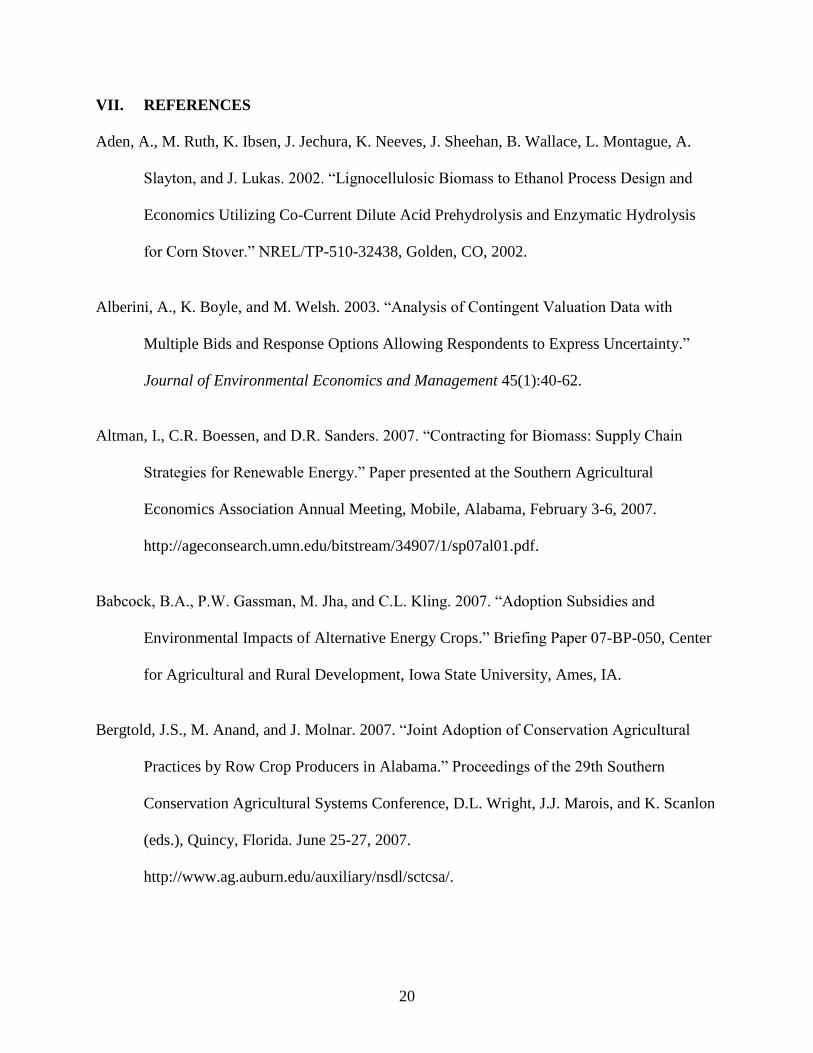
feedstock. The model showed a sensitivity of 97.8% and specificity of 88.3% for a farmer‟s

decision to grow cover crops as a biofuel feedstock. The detailed results of the PROBIT model

for this stage are presented in table 1.3.

Farmers who participate in the federal conservation programs such as CSP and

EQIP are more likely to grow cover crops as a biofuel feedstock as they may already have

experience in managing cover crops. Being enrolled in a federal conservation program can

increase the likelihood of a farmer‟s willingness to grow cover crops a biofuel by 42% (EQIP) to

73% (CSP) Furthermore, if farmers can remove only a portion of the cover crop biomass to get

additional revenue while continuing to qualify for conservation programmatic payments, then

conservation payments may provide a mechanism for risk-averse farmers to cover part of the

risk-premium for adopting this practice. Farmers who have a greater percentage of their farming

3 Information obtained from the survey conducted. Out of 317 respondents only 211 had grown cover crops in the

last 3 years. Average cover crops acreage was only 217 acres as compared to row crop acreage of 763 acres. It is

assumed that the survey findings are representative of the entire sample.

15

land involved in row crop operations are 65% more likely to grow cover crops as a biofuel

feedstock given the potential revenue gain.

Farmers growing corn as a cash crop on their farms are more likely to grow cover

crops as a biofuel feedstock. Survey results show that out of 178 farmers who grew corn in 2007,

40% altered their crop rotations to grow more corn due to increased demand for ethanol

production. Farmers growing corn might have sold corn as a biofuel feedstock and are more

likely to be aware of additional revenue generation opportunities by supplying additional

cellulosic biofuel feedstock sources. Results show that farmers growing corn are 34% more

likely to grow cover crops as a biofuel feedstock. Growing a cover crop can help maintain

biomass levels on the soil surface and provide an alternative to harvesting corn stover as a

feedstock source. Those farmers who desire high biomass as an essential cover crop

characteristic have 50% higher likelihood to grow and sell that biomass as a biofuel feedstock.

This characteristic potentially allows farmers to take advantage of partial stover removal, while

reaping some of the conservation benefits from leaving residue on the soil surface. Furthermore,

the amount of biomass generated by the cover crop is directly related to the amount of revenue

the farmer will earn from selling it.

Some farmers perceive the high cost of cover crops as a disadvantage. These

farmers may be aware of the benefits of cover crops, but are hesitant to grow them for financial

reasons. For this reason, farmers are more likely to grow cover crops as a biofuel feedstock to

offset the costs associated with cover crop adoption. Farmers who perceived cover crops as a

high cost enterprise are 19 percent more likely to adopt them as a biofuel feedstock source.

Those farmers who are of the opinion that cover crops help in increasing cash crop yields are

also more likely to grow them as a biofuel feedstock by 39%. This would enable them to first

16

reap the benefit of increased cash crop yields and then gain additional revenues by partial stover

removal. Given the fluctuations in commodity prices over the past ten years, any additional

income streams that help to stabilize income are likely to be more favorable to farmers.

Those farmers who are not willing to grow cover crops for agronomic reasons

such as interference with cash crops are less likely to engage themselves in growing them as a

biofuel feedstock due to their unfavorable past experiences. Results show that these farmers are

64% less likely to grow cover crops as biofuel feedstock. Similarly those farmers who are not

willing to grow cover crops for production or economic reasons are less likely to grow cover

crops to be used as a biofuel feedstock by 90%. Also, those farmers who have low debt are less

likely (25%) to grow cover crops as a biofuel feedstock due to their unwillingness to acquire

more debt (by investing in a new opportunity).

Elicitation Stage:

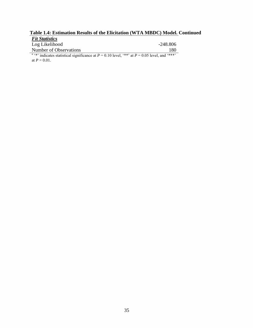
In the second stage, the elicitation model is used to predict the mean willingness

to accept price for cover crop biomass to be sold as a biofuel feedstock. The model (see table1.4)

evaluates the factors that affect the price at which the farmer would be willing to sell the cover

crop biomass as the biofuel feedstock. The model further predicts that mean WTA is $54.62 per

dry ton with an estimated standard error of $7.93, which is in line with the predicted prices in the

literature. Aden et al., (2002) predicted a delivered price of $62 per ton to the refinery of which

$14 was transportation costs, resulting in a selling price of $48 by the farmer. Brechbill and

Tyner (2008) have calculated biomass costs to range between $39 and $46 for corn stover and

$57 and $63 for switchgrass.

A number of factors affect a farmer‟s WTA or price at which they would sell

cover crop biomass as a biofuel feedstock source. Farmers who are enrolled in the EQIP program

17

are more likely to sell biomass at a higher price. Under the EQIP program in Alabama, farmers

are paid ($20/acre) for the introduction of re-seeding legumes into high residue conservation

tillage systems4. Thus these farmers would lose their EQIP payments for growing non-legume

cover crops as a biofuel feedstock and would demand a higher selling price to make it financially

feasible for them.

However, those farmers who are enrolled in the CSP program can receive

enhancement payments from the program for growing cover crops and maintain higher levels of

residue cover on the soil surface. Given that the farmers may be able to remove a portion of the

biomass and still meet the stated eligibility requirements, WTA for CSP participants is not as

high. In addition, the payments from the CSP for cover crop adoption cover a portion of the

production costs. Thus, these farmers have an opportunity to generate supplemental income and

would be willing to sell biomass at a lower price.

Farmers with high income are likely to sell biomass at higher prices as they would

engage in a new activity only if it results in significant revenue addition. Also, they may require

a more significant commitment in resources and a larger management effort to undertake a new

practice. Those farmers who desire high biomass as a cover crop characteristic for conservation

purposes are likely more aware of the benefits of leaving biomass on the field. These farmers are

likely to sell biomass at a higher price to compensate for the loss in agronomic and

environmental benefits. Farmers with prior experience growing cover crops are likely to sell at a

lower price as they are already have experience growing cover crops and can more easily adapt

their operations to the new enterprise at less cost. Farmers who are of the opinion that cover

crops help in increasing cash crop yields would sell biomass at a higher price as they might

4 Alabama EQIP practice and Payment Schedule. 2008

18

perceive a loss in yields by removing cover crop biomass. Older farmers are more likely to sell

biomass at a higher price as they may be less willing to invest in a new enterprise, where as those

farmers with at least a college education would be in a better position to compare the costs and

benefits, potentially resulting in them willing to sell biomass at lower prices.

VI. CONCLUSIONS

The market for cellulosic feedstocks is still in the developing stage. The paper

estimates a two-stage model using farmer data from Alabama to estimate farmer‟s willingness to

produce cover crops as a cellulosic biofuel feedstock. The first stage examines the farmer‟s

willingness to produce and sell cover crop biomass as a biofuel feedstock. Results show that

farmers enrolled in conservation plans such as EQIP or CSP, those who have grown corn in last

3 years, have a higher percentage of acreage in the row crop operations, desiring high biomass

from cover crops and those who perceive high cost of cover crop as a problem are more likely to

grow cover crops as biofuel feedstock. Those farmers who have low debt or are not growing

cover crops due to agronomic, production or economic reasons are less likely to adopt this

practice.

The second stage examines the price at which a farmer would be willing to sell

their cover crop biomass as biofuel feedstock. Model results indicate that using cover crops

residues as a biofuel feedstock can provide an extra revenue generation opportunity for the

farmers. Farmers may be willing to add this extra revenue generation opportunity in their

cropping systems. Farmers enrolled in EQIP, having high income, desiring high biomass as a

cover crop characteristic, believing that cover crop increases cash crop yield and are of higher

age are more likely to sell cover crop biomass at a higher price. On the other hand, those enrolled

19

in CSP, have higher percent of land rented, gown cover crop in last three years or have college

education would be willing to sell cover crop biomass at a lower price.

Fifty-seven percent of the farmers surveyed have shown their willingness to

produce a cover crop for biofuel production. Thus the results have reconfirmed the belief that

cover crops could prove to be a sustainable source of cellulosic ethanol. The predicted mean

willingness to accept price ($54.62) for the cover crop biomass is in line with the current market

prices and signifies an acceptance both from the seller and buyer perspective.

The results of this model provide an insight into a market which is still in the

developing stage and show that selling cover crop biomass as biofuel feedstock is feasible and

farmers are willing to adopt this practice. Refineries would only be interested in establishing a

plant if they are able to get a sustainable supply. Also, farmers would be willing to change their

cropping patterns if they foresee a long-term revenue gain. Further, research is needed to

understand and develop the contractual framework between the farmers and the refineries. More

research also needs to be conducted into actual harvesting practices that would maximize the

economic and agronomic benefits from cover crops.

20

VII. REFERENCES

Aden, A., M. Ruth, K. Ibsen, J. Jechura, K. Neeves, J. Sheehan, B. Wallace, L. Montague, A.

Slayton, and J. Lukas. 2002. “Lignocellulosic Biomass to Ethanol Process Design and

Economics Utilizing Co-Current Dilute Acid Prehydrolysis and Enzymatic Hydrolysis

for Corn Stover.” NREL/TP-510-32438, Golden, CO, 2002.

Alberini, A., K. Boyle, and M. Welsh. 2003. “Analysis of Contingent Valuation Data with

Multiple Bids and Response Options Allowing Respondents to Express Uncertainty.”

Journal of Environmental Economics and Management 45(1):40-62.

Altman, I., C.R. Boessen, and D.R. Sanders. 2007. “Contracting for Biomass: Supply Chain

Strategies for Renewable Energy.” Paper presented at the Southern Agricultural

Economics Association Annual Meeting, Mobile, Alabama, February 3-6, 2007.

http://ageconsearch.umn.edu/bitstream/34907/1/sp07al01.pdf.

Babcock, B.A., P.W. Gassman, M. Jha, and C.L. Kling. 2007. “Adoption Subsidies and

Environmental Impacts of Alternative Energy Crops.” Briefing Paper 07-BP-050, Center

for Agricultural and Rural Development, Iowa State University, Ames, IA.

Bergtold, J.S., M. Anand, and J. Molnar. 2007. “Joint Adoption of Conservation Agricultural

Practices by Row Crop Producers in Alabama.” Proceedings of the 29th Southern

Conservation Agricultural Systems Conference, D.L. Wright, J.J. Marois, and K. Scanlon

(eds.), Quincy, Florida. June 25-27, 2007.

http://www.ag.auburn.edu/auxiliary/nsdl/sctcsa/.

21

Bergtold, J.S., P.A. Duffy, D. Hite, and R.L. Raper. 2008. “Demographic and Management

Factors Affetcing the Perceived Benefit of Winter Cover Crops.” in the Southeast

American Agricultural Economics Association, Orlando, FL, July 28-29, 2008.

Bransby, D.I. 1998. “Interest Among Alabama Farmers in Growing Switchgrass for Energy.”

Paper presented at BioEnergy ‟98: Expanding Bioenergy Partnerships, Madison,

Wisconsin, October 4-8, 1998. http://bioenergy.ornl.gov/papers/bioen98/bransby1.html.

Brechbill, S., and W. Tyner. 2008. “The Economics of Biomass Collection, Transportation, and

Supply to Indiana Cellulosic and Electric Utility Facilities.” Purdue University,

Department of Agricultural Economics, Working Paper #08-03.

http://ageconsearch.umn.edu/bitstream/6148/2/wp080003.pdf.

Cameron, T. A., G. L. Poe, R. G. Ethier, and W.D. Schulze. 2002. “Alternative Nonmarket

Value-Elicitation Methods: Are Revealed and Stated Preferences the Same?” Journal of

Environmental Economics and Management 44(3):391-425.

Calia, P., and E. Strazzera. 1999. “Sample Selection Model for Protest Votes in Contingent

Valuation Analyses.” FEEM Working Paper No. 55.99. http://ssrn.com/abstract=200620

Clark, A. (Editor). 2007. “Managing Cover Crops Profitably.” Third Edition, Handbook Series

Book 9. Beltsville, MD: Sustainable Agriculture Network.

Creamer, N.G., M.A. Bennet, B.R. Stinner, J. Cardina, and E.E. Regnier. 1996. “Mechanisms of

Weed Suppression in Cover Crop Based Production Systems.” Hortscience 31:410-413.

22

Dabney, S.M., and D.W. Reeves. 2001. “Using Winter Cover Crops to Improve Soil and Water

Quality.” Communications in Soil Science and Plant Analysis 37:1221-1250.

de la Torre Ugarte, D.G., B.C. English, and K. Jensen. 2007. “Sixty Billion Gallons by 2030:

Economic and Agricultural Impacts on Ethanol and Biodiesel Expansion.” American

Journal of Agricultural Economics 89:1290-1295.

Efron, B. and R.J. Tibshirani. 1986. “An Introduction to the Bootstrap.” Monograms on Statistics

and Applied Probability. 57, Chapman Hall, New York, NY.

Epplin, F.M., C.D. Clark, R.K. Roberts, and S. Hwang. 2007. “Challenges to the Development of

a Dedicated Energy Crop.” American Journal of Agricultural Economics 89:1296-1302.

Featherstone, A.M., and B.K. Goodwin. 1993. “Factors Influencing a Farmer's Decision to Invest

in Long Term Conservation Improvements.” Land Economics 69:67-81.

Gallagher, P.W., M. Dikeman, J. Fritz, E. Wailes, W. Gauthier, and H. Shapouri. 2003. “Supply

and Social Cost Estimates for Biomass from Crop Residues in the United States.”

Environmental and Resource Economics 24:335-358.

Glassner, D.A., J.R. Hettenhaus, and T.M. Schechinger. 1998. “Corn Stover Collection Project.”

Paper presented at BioEnergy‟98: Expanding Bioenergy Partnerships, Madison,

Wisconsin, October 4-8, 1998.

http://ergosphere.files.wordpress.com/2007/04/bio98_corn_stover.pdf.

23

Gould, B.W., W.E. Saupe, and R.M. Klemme. 1989. “Conservation Tillage: The Role of the

Farm and Operator Characteristics and the Perception of Soil Erosion.” Land Economics

65:167-182.

Graham, R.L. 1994. “An Analysis of the Potential Land Base for Energy Crops in the

Conterminous United States.” Biomass and Bioenergy 6:175-189.

Graham, R.L., R. Nelson, J. Sheehan, R.D. Parlack, and L.L. Wright. 2007. “Current and

Potential U.S. Corn Stover Supplies.” Agronomy Journal 99:1-11.

Greene, W.H. 2003. Econometric Analysis, fifth ed. Macmillan, New York.

Halstead, J.M., A.E. Luloff, and T.H. Stevens. 1992. “Protest Bidders in Contingent

Valuation.” Northeastern Journal of Agricultural Economics 21:160-169.

Heckman, J.J. 1979. “Sample Selection Bias as a Specification Error.” Econometrica 47:153-

161.

Heid, W.G. Jr. 1984. “Turning the Great Plains Crop Residues and Other Products into Energy.”

In: (revised 2nd edn. ed.), Economics Research Service Agricultural Economic Report

No. 523, U.S. Department of Agriculture (November 1984).

Hennessy, D.A. 2006. “On Monoculture and Structure of Crop Rotations.” American Journal of

Agricultural Economics 88:900-914.

24

Hipple, P.C., and M.D. Duffy. 2002. “Farmers‟ Motivations for Adoption of Switchgrass.” in J.

Janich and A. Whipkey eds. Trends in New Crops and New Uses. ASHA Press,

Alexandria, VA, pg. 252-266.

Jensen, K., C.D. Clark, P. Ellis, B. English, J. Menard, M. Walsh, and D. de la Torre Ugarte.

2007. “Farmer Willingness to Grow Switchgrass for Energy Production.” Biomass and

Bioenergy 31:773-781.

Kelsey, K.D., and T.C. Franke. 2009. “The Producers' Stake in the Bioeconomy: A Survey of

Oklahoma Producers' Knowledge and Willingness to Grow Dedicated Biofuel Crops.”

Journal of Extension 47(1) 1RIB5.

http://www.joe.org/joe/2009february/pdf/JOE_v47_1rb5.pdf.

Larson, J.A., B.C. English, and L. Lambert. 2007. “Economic Analysis of the Conditions for

Which Farmers Will Supply Biomass Feedstocks for Energy Production.” Final Report

for Agricultural Marketing Center Special Projects Grant 412-30-54, Agricultural

Marketing Resource Center, University of Tennessee.

http://www.agmrc.org/media/cms/2007UTennProjDeliverable_9BDDFC4C2F4E5.pdf.

Lichtenberg, E. 2004. “Cost-Responsiveness of Conservation Practice Adoption: A Revealed

Preference Approach.” Journal of Agricultural and Resource Economics 29(3):420-435.

Loomis, J., and E. Ekstrand. 1997. “Economic Benefits of Critical Habitat for the Mexican

Spotted Owl: A Scope Test Using a Multiple-Bounded Contingent Valuation Survey.”

Journal of Agricultural and Resource Economics 22(2):356-366.

25

Lotter, D.W., R. Seidel, and W. Liebhardt. 2003. “The performance of Organic and Conventional

Cropping Systems in an Extreme Climate Year.” American Journal of Alternative

Agriculture 18:146-154.

Maddala, G.S. 1983. “Limited-dependent and Qualitative Data in Econometrics.” Cambridge

University Press.

Perlack, R.D., L.L. Wright, A.F. Turhollow, R.L. Graham, B.J. Stokes, and D.C. Erbach. 2005.

“Biomass as Feedstock for a Bioenergy and Bioproducts Industry: The Technical

Feasibility of a Billion-Ton Annual Supply.” Washington, DC: U.S. Department of

Agriculture and U.S. Department of Energy.

Rajagopal, D., and D. Zilberman. 2007. “Review of Environmenal, Economic and Policy

Aspects of Biofuels.” Policy Research Working Paper 4341, World Bank, Washington,

D.C.

Raper, R.L., E.B. Schwab, J.S. Bergtold, A.J. Price, K.S. Balkcom, F.J. Arriaga, and T.S.

Kornecki. 2009 “Maximizing Cotton Production and Rye Cover Crop Biomass through

Timely In-Row Subsoiling.” Applied Engineering in Agriculture 25:321-328.

Reeves, D.W. 1994. “Cover Crops and Rotations.” In J. L. Hartfield and B. A. Stewart, eds.

Advances in Soil Science: p. 125-172, Crop Residue Management. Lewis Publishers,

CRC Press, Boca Raton, FL.

26

Roberts, R.K., J.A. Larson, D.D. Tyler, B.N. Duck, and K.D. Dillivan. 1998. “Economic

Analysis of the Effects of Winter Cover Crops on No-Tillage Corn Yield Response to

Applied Nitrogen.” Journal of the Soil and Water Conservation 53:280-284.

Rosillo-Calle, F., P. de Groot, S.L. Hemstock, and J. Woods. (eds) 2007. “The Biomass

Assessment Handbook: Bioenergy for a Sustainable Environment.” London: Earthscan

Rowe, R., W. Schulze, and W. Breffle. 1996. “A Test for Payment Card Biases.” Journal of

Environmental Economics and Management 31:178-185.

Singer, J.W. 2008. “Corn Belt Assessment of Cover Crop Management and Preferences.”

Agronomy Journal 100:1670-1672.

Singer, J.W., S.M. Nusser, and C.J. Alf. 2007. “Are Cover Crops Being Used in the US Corn

Belt?” Journal of Soil and Water Conservation 62(5):353-358.

Snapp, S.S., S.W. Swinton, R. Labarta, D. Mutch, J.R. Black, R. Leep, J. Nyiraneza, and K.

O'Neal. 2005. “Evaluating Cover Crops for Benefits, Costs and Performance with in

Cropping System Niches.” Agronomy Journal 97:322-332.

Soule, M.J., A. Tegene, and K.D. Wiebe. 2000. “Land Tenure and Adoption of Conservation

Practices.” American Journal of Agricultural Economics 82:993-1005.

Soule, M.J. 2001. “Soil Management and the Farm Typology: Do Small Farms Manage Soil and

Nutrient Resources Differently than Large Family Farms?” Agricultural and Resource

Economics Review 30:179-188.

27

Stricker, J.A., S.A. Segrest, D.L. Rockwood, and G.M. Prine. 2000. “Model Fuel Contract: Co-

Firing Biomass with Coal.” Paper presented at the Soil and Crop Science Society of

Florida and Florida Nematology Forum, 60th Annual Meeting, Tallahassee, Florida.

September 20-22, 2000.

http://www.techtp.com/Cofiring/Model%20Contract%20Cofiring%20Biomass%20with%

20Coal.pdf.

Turnhollow, A. 1994. “The Economics of Energy Crop Production.” Biomass and Bioenergy

6:229-241.

Uri, N.D. 1999. “Factors Affecting the Use of Conservation Tillage in the United States.” Water

Air Soil Pollution 116:621-638.

USDA Agricultural Census, 2007. Alabama.

http://www.agcensus.usda.gov/Publications/2007/Full_Report/Volume_1,_Chapter_1_St

ate_Level/Alabama/st01_1_009_010.pdf.

Walsh, M.E., D.G. de la Torre Ugarte, H. Shapouri, and S.P. Slinsky. 2003. “Bioenergy Crop

Production in the United States.” Environmental and Resource Economics 24:313-333.

Welsh, M.P., and R.C. Bishop. 1993. “Multiple Bounded Discrete Choice Models.” in W-133

Benefits and Costs Transfer in Natural Resource Planning, Western Regional Research

Publication compiled by J. Bergstrom, Dept. of Ag. and Applied Economics, University

of Georgia.

28

Welsh, M.P., and G.L. Poe. 1998. “Elicitation Effects in Contingent Valuation: Comparisons to a

Multiple Bounded Discrete Choice Approach.” Journal of Environmental Economics and

Management 36:170-185.

Wilhelm, W.W., J.M.F. Johnson, J.L. Hatfield, W.B. Voorhees, and D.R. Linden. 2004. “Crop

and Soil Productivity Response to Corn Residue Removal: A Literature Review.”


Wu, J.J., and B.A. Babcock. 1998. “The Choice of Tillage, Rotation and Soil Testing Practices;

Economic and Environmental Implications.” American Journal of Agricultural

Economics 80:494-511.

29

Table 1.1: Summary Statistics for Survey Respondents and Sample Population.

Variable Survey Population

Age 55.7 58.1

Gross Farm Sales

<$50,000 10.5% not sampled

$50,000-$99,999 19.5% 10.2%

$100,000-$249,999 29.0% 32.7%

$250,000-$499,999 21.3% 25.8%

$500,000-$999,999 11.7% 19.9%

> $ 1 Million 8.1% 11.5%

Race

White or Caucasian 98.2% 96.4%

Black or African American 0.9% 1.7%

American Indian 0.9% 0.9%

All others 0% 1%

Row Crop Acreage 753 acres 878 acres

Total Acreage Source: Agricultural Census 2002, USDA-NASS

30

Table 1.2: Variable Description for Cover Crop Adoption Model (N = 317).

Variable Description Mean/

Frequencya

Conservation Participation

Conservation

Plan

1, if farmer has a conservation plan on his farm, 0

otherwise 78.23%

EQIP 1, if farmer participates in the EQIP program, 0

otherwise 43.22%

CSP 1, if farmer participates in the CSP program, 0

otherwise 5.68%

CT 1, if farmer uses conservation tillage on his farm, 0

otherwise 77.92%

Farm Characteristics

Percent Row Percent of land in the row crop operations 70

(0.3)

Percent Rent Percentage of land rented by the farmer 60

-0.3

Corn 1, if farmer has grown corn in the last 3 years, 0

otherwise 64.04%

Cotton 1, if farmer has grown cotton in the last 3 years, 0

otherwise 63.72%

Peanuts 1, if farmer has grown peanuts in the last 3 years, 0

otherwise 45.43%

Soybeans 1, if farmer has grown soybeans in the last 3 years,

0 otherwise 41.96%

Income Average yearly gross sales chosen from six given

intervals

3.4

(1.4)

Farmer Perception of Cover Crops

Info Cover

crops

1, if farmer has enough information to make cover

crop decisions, 0 otherwise 73.19%

High Biomass 1, if farmer desires high biomass as a cover crop

characteristic, 0 otherwise 17.98%

Nitrogen

Fixation

1, if farmer desires nitrogen fixation as a cover crop

characteristic, 0 otherwise 39.12%

High Cost 1, if farmer perceives high cost as a disadvantage

for cover crops, 0 otherwise 53.31%

Harvest-Graze 1, if farmer harvests or grazes the cover crop, 0

otherwise 33.75%

Grown Cover

Crops in 3

Years

1, if farmer has grown cover crops at least once in

last three years, 0 otherwise 66.56%

Receive Cover

Crop Cost

share

1, if receives some cost share assistance for

growing cover crops, 0 otherwise 15.77%

31

Table 1.2: Variable Description for Cover Crop Adoption Model (N = 317). Continued

Increase Cash

Crop Yield

1, if farmer thinks that cover crops increases cash

crop yields, 0 otherwise 31.23%

Not WTG

Agronomy

1, if farmer doesn‟t grow cover crops for

agronomic reasons, 0 otherwise 11.67%

Not WTG

Prod-Econ

1, if farmer doesn‟t grow cover crops for

production/economic reasons, 0 otherwise 32.49%

Demographics

Low Debt 1, if farmer perceives having low debt, 0 otherwise 54.26%

Off farm

employment

1, if one or more members of the family work off-

farm, 0 otherwise 51.42%

Age Farmer‟s Age 55.4

(11.3)

College 1, if farmer has at least some college education, 0

otherwise 58.99%

a For discrete data frequency of response is reported. For continuous variables the standard deviation is reported in

parenthesis

32

Table 1.3: Estimation Results for the Selection PROBIT Model.

Variable

Parameter

Estimatea

(Standard Error)

Marginal Effecta

(Standard Error)

Intercept 0.4608 0.1712

(1.3153) (0.4873)

Conservation plan -0.4681 -0.1797

(0.3984) (0.1533)

EQIP 1.1693 *** 0.4241 ***

(0.4463) (0.1496)

CSP 3.9809 *** 0.7264 ***

(1.5412) (0.1031)

CT 0.5324 0.1834

(0.3657) (0.1150)

Percent Row 1.7520 *** 0.6510 ***

(0.6777) (0.2522)

Percent Rent -0.3848 -0.1430

(0.5589) (0.2059)

Corn 1.0133 *** 0.3425 ***

(0.3696) (0.1176)

Cotton 0.5040 0.1805

(0.3821) (0.1312)

Peanuts 0.1188 0.0442

(0.3956) (0.1484)

Soybeans 0.0147 0.0054

(0.3787) (0.1408)

Income -0.1447 -0.0538

(0.1469) (0.0546)

Info Cover crops 0.0293 0.0109

(0.3551) (0.1314)

High Biomass 1.3713 ** 0.5062 ***

(0.5638) (0.1745)

Nitrogen Fixation -0.1027 -0.0380

(0.3284) (0.1213)

High Cost 0.5277 * 0.1929 *

(0.3192) (0.1144)

Harvest-Graze 0.7033 0.2659

(0.5146) (0.1928)

33

Table 1.3: Estimation Results for the Selection PROBIT Model. Continued

Grown Cover Crops in last 3

Years

-0.3557 -0.1343

(0.4964) (0.1905)

Receive Cover Crop Cost

share

0.3702 0.1424

(0.8744) (0.3430)

Increase Cash Crop Yield 1.0294 ** 0.3872 **

(0.4874) (0.1745)

Not WTG Agronomy -6.3292 *** -0.6412 ***

(1.6292) (0.0918)

Not WTG Prod-Econ -5.0347 *** -0.8959 ***

(0.8935) (0.0422)

Low Debt -0.6621 * -0.2446 *

(0.3622) (0.1335)

Off farm employment -0.2943 -0.1092

(0.3547) (0.1303)

Age -0.0226 -0.0084

(0.0152) (0.0056)

College 0.2746 0.1008

(0.3414) (0.1250)

Fit Statistics

Log Likelihood -216.802

R2 .6529

AIC 435.604

Number of

Observations

317

Prediction Success

Sensitivity = actual 1s correctly predicted 97.78%

Specificity = actual 0s correctly predicted 88.32%

Positive predictive value = predicted 1s that were actual 1s 91.67%

Negative predictive value = predicted 0s that were actual 0s 96.80%

Correct prediction = actual 1s and 0s correctly predicted 93.69%

Prediction Failure

False pos. for true neg. = actual 0s predicted as 1s 11.68%

False neg. for true pos. = actual 1s predicted as 0s 2.22%

False pos. for predicted pos. = predicted 1s actual 0s 8.33%

False neg. for predicted neg. = predicted 0s actual 1s 3.20%

False predictions = actual 1s and 0s incorrectly predicted 6.31% a „*‟ indicates statistical significance at P = 0.10 level, „**‟ at P = 0.05 level, and „***‟ at

P = 0.01.

34

Table 1.4: Estimation Results of the Elicitation (WTA MBDC) Model.

Variable WTA Estimatesa(Standard Error)

Intercept 27.8717 *

(18.615)

Lambda -26.9365 **

(12.703)

Conservation plan -5.8618

(5.832)

EQIP 9.5934 **

(4.902)

CSP -12.3264 *

(6.554)

CT 8.2446

(6.064)

Percent Rent -10.8175 *

(7.275)

Corn -3.3398

(5.129)

Cotton 3.2656

(5.037)

Peanuts -1.1042

(4.577)

Soybeans 2.3685

(4.426)

Income 2.9354 *

(1.758)

High Biomass 15.2837 ***

(5.434)

High Cost -1.5526

(4.081)

Harvest-Graze 5.6502

(5.189)

Grown Cover Crops in last 3

Years

-14.0436 **

(6.449)

Receive Cover Crop Cost

share

-3.491

(5.754)

Inc Cash Crop Yield 7.9181 *

(5.205)

Low Debt 5.4312

(4.688)

Off farm employment 1.9862

(3.966)

Age 0.3032 *

(0.205)

College -7.3426 *

(4.349)

35

Table 1.4: Estimation Results of the Elicitation (WTA MBDC) Model. Continued

Fit Statistics

Log Likelihood -248.806

Number of Observations 180 a „*‟ indicates statistical significance at P = 0.10 level, „**‟ at P = 0.05 level, and „***‟

at P = 0.01.

36

30. If you could (or already do) incorporate a cover crop into your current

production system, would you be willing to produce a cover crop for biofuel

production?

___ Yes

(Please answer question 30a)

___ No

(if NO, please SKIP to question 30b)

30a. If yes, consider the option of growing a rye or wheat cover crop for ethanol

production on your farm. The yearly average amount of biomass produced by

such a cover crop for this purpose would be 4 to 6 tons per acre (dry-weight). The

table below provides different prices per ton of cover crop biomass (dry-weight)

that a bio-refinery might pay for this residue. For each price, indicate your

willingness to produce a cover crop for ethanol production at the given price.

Price of cover crop

biomass ($/ton)

Would you produce and sell the cover crop

biomass/residue to a bio-refinery for ethanol production?

(Please circle one answer for each row)

$15 Yes No Do not know




30b. If no, why are you not willing to grow a cover crop for biofuel production?

(Mark all that apply)

__ Too risky __ Not enough time __ Lower soil productivity

__ Lower crop yields __Lower soil organic matter __ Less soil protection

__ Costs too high __Not enough information __ Other (specify): ______

Figure 1.1: Selection and Elicitation (MBDC) Question from Survey

37

APPENDIX 1: SURVEY

Cover Crop Use on Southeastern Farms

A Survey of Conservation Practices, Cover Crop, and Biofuel Adoption

We need your help to improve the conservation research, programs and services that farmers

receive from USDA-NRCS, other federal agencies, and state institutions, such as Auburn

University.

Your views and experiences on conservation practices, cover crops, and biofuels will be

summarized and used to recommend ways to improve conservation programs and services

available to Alabama farmers, as well as to guide conservation agricultural research efforts

that help to sustain and improve farming in Alabama.

The USDA – Agricultural Statistics Service has randomly selected names to be included in

this study. Your name and responses will remain strictly confidential. The information

you provide will be combined with reports from other farmers for statistical purposes.

Auburn University will complete the final report for USDA.

Enclosed with this survey you will find an information sheet about cover crops in

conservation systems and their potential as a biofuel feedstock. Please examine this sheet for

your information and as a resource for the survey.

Please complete the survey as soon as possible and return it in the enclosed envelope which

does not need a stamp. Thank You.

Contact: Patricia Duffy, Department of Agricultural Economics and Rural Sociology,

Auburn University, (334) 844-5629, email: [email protected].

38

CONSERVATION ON YOUR FARM

1. Do you have a conservation plan for your farm? 101 ___Yes1 ___ No

2

2. Do you participate in any of the following conservation programs administered by the USDA Natural Resources

Conservation Service (NRCS)? (Mark all that apply)

102 ___ Environmental Quality Incentives (EQIP) 103 ___ Conservation Reserve Program (CRP)

104 ___ Conservation Security Program (CSP) 105 ___ Other (specify):____________________

3. Do you use any of the following conservation practices?

Conservation Practice Do you use this practice?

Have you received cost-

share, incentive payments or

income for using this

practice?

Conservation Tillage 106

___ Yes1 ___ No

2

107

___ Yes1 ___ No

2

Filter or Buffer Strips 108

___ Yes1 ___ No

2

109

___ Yes1 ___ No

2

Wildlife Habitat 110

___ Yes1 ___ No

2

111

___ Yes1 ___ No

2

Precision Agriculture

(Site-Specific, GPS, etc.) 112

___ Yes1 ___ No

2

113

___ Yes1 ___ No

2

Crop Nutrient Management 114

___ Yes1 ___ No

2

115

___ Yes1 ___ No

2

Integrated Pest Management 116

___ Yes1 ___ No

2

117

___ Yes1 ___ No

2

4. Where do you get information about conservation practices for your farm? (Mark all that apply)

118 ___ Extension Service 119 ___ State Universities

120 ___ Internet 121 ___ Books, journals, magazines, flyers

122 ___ Field days/workshops 123 ___ Other farmers

124 ___ USDA - Agricultural Research Service (ARS) 125 ___ USDA – NRCS

FARMING OPERATION

5. Of the total land you operate, how many acres are used:

a. to grow row crops? ……………….201 _________ acres

b. for hay or forage production? ……202 _________ acres

c. as pasture for grazing livestock?...203 _________ acres

39

6. Considering the total land in your farming operation, how many acres:

a. are owned by you?............................................................................ 204 _________ acres

b. rented from others, including land used rent free?............................ 205 _________ acres

7. How many separate parcels of land do you operate?............................ 206 _________ parcels

8. Do you irrigate your crops? 207 ___ Yes1 ___ No

2

9. What is your typical crop rotation(s)? (Please describe) 208

____________________________________________________________________________________

10. What major crops are grown on your farm? Please indicate whether you have planted the listed crops in the past

3 years and the number of acres planted in 2007; also, indicate the predominant type of tillage practice(s) used for

that crop during this period of time. In-row subsoiling refers to tillage practices such as Strip-till and Paratill that

leave the majority of crop residues on the soil surface.

Crop

Grown in the past 3

years?

Acres Planted in

2007

Predominant Tillage Practice(s)

used over the past 3 years

(Circle all that apply)

1 - No Tillage

2 - In-row Subsoiling

3 - Disc / Chisel

4 - Moldboard Plow

5 – Other (if other, please specify)

a. Corn 209

___ Yes1 ___ No

2

210

_______ ac

211

1 2 3 4 5 _____________

b. Cotton 212

___ Yes1 ___ No

2

213

_______ ac

214

1 2 3 4 5 _____________

c. Peanuts 215

___ Yes1 ___ No

2

216

_______ ac

217

1 2 3 4 5 _____________

d. Soybeans 218

___ Yes1 ___ No

2

219

_______ ac

220

1 2 3 4 5 _____________

e. Wheat 221

___ Yes1 ___ No

2

222

_______ ac

223

1 2 3 4 5 _____________

f. Hay/Forage

Crops

224

___ Yes1 ___ No

2

225

_______ ac

226

1 2 3 4 5 _____________

g. Other

(specify)-

227

___ Yes1 ___ No

2

228

_______ ac

229

1 2 3 4 5 _____________

40

11. Including sales of crops, livestock, poultry and miscellaneous agricultural products (including the landlord‟s

share) and government agricultural payments over the past 3 years, which category represents the average yearly

total gross value of sales from this operation? (Mark one)

230 ___ Less than $50,0001 ___ $50,000 to $99,999

2 ___ $100,000 to $249,999

3

___ $250,000 to $499,9994 ___ $500,000 to $999,999

5 ___ $1,000,000 and over

6

11a. What percentage of sales in Question #11 comes from row crop production? 231 _________ %

COVER CROPS (Please read the flyer that accompanied the survey about cover crops)

12. Do you think you have enough information about cover crops to make decisions about cover crop selection, use

and management?

301 ____ Yes1

____ No2

13. Have you received information about crop selection, use or management from any of the following sources?

Source of Information Received Cover Crop

Information?

If yes, was the information

helpful?

a. Local Co-op 302

___ Yes1 ___ No

2

303

___ Yes1 ___ No

2

b. Other Farmers 304

___ Yes1 ___ No

2

305

___ Yes1 ___ No

2

c. Agribusinesses, such as seed or

chemical companies 306

___ Yes1 ___ No

2

307

___ Yes1 ___ No

2

d. University and/or Extension 308

___ Yes1 ___ No

2

309

___ Yes1 ___ No

2

e. National Resource

Conservation Service (NRCS) 310

___ Yes1 ___ No

2

311

___ Yes1 ___ No

2

g. Agricultural Research Service

(ARS) 312

___ Yes1 ___ No

2

313

___ Yes1 ___ No

2

14. If you were to (or already do) plant cover crops, what plant characteristics would you desire? (Mark all that

apply)

314 ___ Fall Residue Cover 315 ___ Spring Residue Cover 316 ___ Nitrogen Fixation

317 ___ High Biomass Production 318 ___ Early Season Bloom 319 ___ Other (specify):______

15. What would you say are the advantages of using cover crops prior to growing your cash crop? (Mark all that

apply)

320___ No benefits 321 ___ Reduces soil erosion 322 __ Increases water storage

323 ___ Increases soil organic matter 324 ___ Suppresses weeds 325 __ Reduces soil compaction

326 ___ Increases yield 327 ___ Increases profitability 328 ___ Lowers pest incidence

329 ___ Reduces production risk 330 ___ Decreases runoff 331 ___ Other (specify): ______

41

16. What are the main problems with using a cover crop on your farm? (Mark all that apply)

332 __ No problems 333 __ High cost 334 ___ Problems with weeds

335 __ Hinders spring planting 336 __ Use of more chemicals 337 ___ Reduced yields

338 __ More insect problems 339 __ Disease problems 340 ___ Depletes soil nutrients

341 __ Depletes soil moisture 342 __ Too risky 343 ___ Other (specify): ________

EXPERIENCE WITH COVER CROPS

17. Have you planted a cover crop in the past THREE years? 401 ___ Yes1

___ No2 (If No, Skip to Question #27,

next pg.)

17a. If YES, please indicate the type(s) of cover crops used and record the seeding rate, seed cost per acre,

amount of nitrogen applied per acre (if applicable), and the cash crop planted afterward.

Cover Crop

(Please specify

cover crop type

and/or mixture)

Grown in the past 3

years?

Seeding

Rate

(lbs/acre)

Seed

Cost

($/acre)

Nitrogen

Fertilizer

Applied

(lbs/acre)

Cash Crop(s)

Planted After

Cover Crop

Example: Rye _X_Yes ___No 90 $22 30 Cotton

402

_____________

403

___ Yes1 ___No

2

404

_______

405

_______

406

_______

407

____________

408

______________

409

___ Yes1 ___No

2

410

_______

411

_______

412

_______

413

____________

414

______________

415

___ Yes1 ___No

2

416

_______

417

_______

418

_______

419

____________

Examples of cover crops include: Wheat, Rye, Oats, Triticale, Crimson Clover, Red Clover, Hairy Vetch,

Ryegrass, Millet, & Other mixtures (such as Wheat / Rye mixes).

18. How many acres did you plant in cover crops during the 2006-2007 growing season? 420 _____ acres

19. What method do you usually use to plant your cover crops? (Mark one)

421 __ Grain drill1 _ Aerial Seeding

2 __Broadcast

3 _ Custom Hire

4 _ Other

5 (specify): ________

20. How do you terminate or kill off your cover crops? (Mark all that apply)

422 ___ Tillage1 ___ Chemical

2 (Burndown) ___ Crimper/Roller

3

21. How long do you wait after killing the cover crop to plant a cash crop? (Mark one)

423 ___ 1 week1 ___ 2 weeks

2 ___ 3 weeks

3 ___ 4 or more weeks

4

22. Do you harvest or graze your cover crop? (Mark one)

424 ___ Harvest for feed or grain1 ___ Winter Annual Graze

2 ___ Neither

3

42

23. If you plant a legume cover crop, do you decrease the amount of nitrogen applied to your cash crop? (Mark one)

425 ___ Yes1

___ No2 ___ Do not plant legume cover crops

3

24. Do you try to produce as much biomass as possible from your cover crop in order to get as much residue as

possible on the soil surface?

426 ___ Yes1 ___ No2 24a. If yes, how high do you grow your cover crop(s)?

427 _____ feet: Type of cover crop: 428 ____________________________

429 _____ feet: Type of cover crop: 430 ____________________________

25. Have you experienced an increase in cash crop yield after using a cover crop?

431 __Yes1 (Go to Question 25a) __ No

2, I experienced a decrease or no change in cash crop yield.

25a. If yes, what crops and by how much did yield increase?

Crop: 432_________________ increased by 433________________ %

Crop: 434_________________ increased by 435________________ %

26. Have you received any cost sharing incentives for using cover crops? 436 ___Yes1 ___ No

2

26a. If yes, what was the source of these funds? 437 ____________________________________

WILLINGNESS TO PRODUCE COVER CROPS (If necessary, please read the flyer that

accompanied this survey to assist with answering the following questions)

27. Farmers plant cover crops to help improve cash crop productivity and yields. The following questions will

present different possible costs of planting a cash crop and will ask you to mark the smallest acceptable gain in yield

that would make it attractive to plant a cover crop at that cost. Or if you would not grow it, please mark "Would not

grow".

a) If the cover crop costs $15 per acre, what is the lowest yield increase from the cash crop that would

make planting a cover crop attractive to you? (Mark one)

501__ 0% __ 5% __ 10% __ 15% __ 20% __Would not grow7

b) If the cover crop costs $30 per acre, what is the lowest yield increase from the cash crop that would


502___ 0% ___ 5% ___ 10% ___ 15% ___ 20% ___ Would not grow7

c) If the cover crop costs $50 per acre, what is the lowest yield increase from the cash crop that would


503___ 0% ___ 5% ___ 10% ___ 15% ___ 20% ___ Would not grow7

d) If the cover crop costs $75 per acre, what is the lowest yield increase from the cash crop that would


504___ 0% ___ 5% ___ 10% ___ 15% ___ 20% ___ Would not grow7

43

BIOFUELS (Please read the flyer that accompanied the survey about biofuels)

28. Do you use ethanol, bio-diesel, or a mixture to operate machinery or vehicles on your farm? (Mark one)

601 ___ Yes1

___ No2 (If NO, Skip to Question #29)

28a. Do you receive cost-share assistance, incentive payments or income for use of these biofuels?

602 ___Yes1 ___ No

2

28b. How available are biofuels for purchase in your area? (Mark one)

603 ___ Readily available1 ___ Somewhat hard to obtain

2

___ Difficult to obtain3 ___ Make my own biofuels

4

29. Did you alter your crop rotations to grow more corn this year due to the increased demand for ethanol

production?

604 ___ Yes1 ___ No

2

WILLINGNESS TO PRODUCE BIOFUEL FEEDSTOCKS (If necessary, please read the flyer

that accompanied this survey to assist with answering the following questions)

30. If you could (or already do) incorporate a cover crop into your current production system, would you be willing

to produce a cover crop for biofuel production?

701 ___ Yes1 (Please answer question 30a) ___ No

2 (if NO, please SKIP to question 30b)

30a. If yes, consider the option of growing a rye or wheat cover crop for ethanol production on your farm. The

yearly average amount of biomass produced by such a cover crop for this purpose would be 4 to 6 tons per acre

(dry-weight). The table below provides different prices per ton of cover crop biomass (dry-weight) that a bio-

refinery might pay for this residue. For each price, indicate your willingness to produce a cover crop for ethanol

production at the given price.

Price of cover

crop biomass ($/ton)

Would you produce and sell the cover crop biomass/residue to a bio-refinery

for ethanol production? (Please circle one answer for each row)

702 $15 Yes1 No

2 Do not know

3

703 $35 Yes1 No

2 Do not know

3

704 $55 Yes1 No

2 Do not know

3

705 $75 Yes1 No

2 Do not know

3

30b. If no, why are you not willing to grow a cover crop for biofuel production? (Mark all that apply)

706 ___ Too risky 707 ___ Not enough time 708 ___ Lower soil productivity

709 ___ Lower crop yields 710 ___ Lower soil organic matter 711 ___ Less soil protection

712 ___ Costs too high 713 ___ Not enough information 714 __ Other (specify): _____

44

BACKGROUND

31. In what year did you begin to operate any part of your farm? 801 __ __ __ __ year [Example 1 9 7 5]

32. Are you or any member of your immediate family living with you employed off the farm? 802 _ Yes __No

32a. If yes, how many family members and how many hours per week on average are they employed off the

farm? 803 _______ family members for 804_______ hours per week.

33. Considering all long-term, short term, secured or unsecured loans, what best describes the current debt level for

your farm? (Mark one)

805 ___ No debt1 ___ Low debt

2 ___ Moderate debt

3 ___ High debt

4

34. What is your (the farm operator‟s) gender? 806 ___ Male1 ___ Female

2

35. How old were you on your last birthday? 807 __________ years

36. What is your race? (Mark one)

808 ___ White or Caucasian1 ___ American Indian

2 ___ Black or African American

3

___ Hispanic4 __ Asian or Pacific Islander

5 ___ Other

6: _________

37. What is the highest level of formal education you have completed? (Mark one)

809 ___ Some high school1 ___ High school or GED equivalency

2 ___ Trade school

3

___ Some college4 ___ College graduate

5 ___ Postgraduate

6

45

COMMENTS

To better understand the needs of farmers, we would like to know what kind of information you may need about

cover crops to make decisions about cover crop selection, use and management. Please provide any feedback you

think is important in the space below.

_____________________________________________________________________________________________

_____________________________________________________________________________________________

_____________________________________________________________________________________________

_____________________________________________________________________________________________

_____________________________________________________________________________________________

_____________________________________________________________________________________________

_____________________________________________________________________________________________

_____________________________________________________________________________________________

_____________________________________________________________________________________________

_______________________________________________________________________________________

_____________________________________________________________________________________________

_____________________________________________________________________________________________

__________________________________________________________________

FOR OFFICE USE ONLY Seq. #

______

Response Respondent Mode Enum. Eval. Date

1-Comp 2-Ref 3-Inacc 4-Office Hold

901 1-Op/Mgr 2-Sp 3-Acct/Bkpr 4-Partner 9-Oth

902 1-Mail 2-Tel 3-Face-to-Face 4-Left w/ Resp

903 904 905 906 DD MM YY

DATE: __ __ __ __ __ __

46

Balancing Feedstock Economics and Ecosystem Services

I. INTRODUCTION

Agro-ecosystems provide a range of services, which from an anthropocentric

view; can be conceptualized as ecosystem services (de Groot et al., 2002). These ecosystem

services have been categorized as: „provisioning‟, „regulating ‟, „cultural‟, and „supporting‟

(Millennium Ecosystem Assessment, 2005). Provisioning services include the production of

food, fiber, feed and fuel. Regulating services include functions that regulate climate, air, water,

and earth surface processes such as greenhouse gas balance, maintenance of the ozone layer, and

regulation of hydrologic flows. Cultural services include aesthetic, spiritual, educational, and

recreational benefits. Supporting services include nutrient cycling, soil formation, crop

pollination, and natural pest control.

Ecosystem services at the farm level have been adversely affected by a number of

factors related to biofuel production. The growing demand for energy, increasing energy costs,

and the need to reduce reliance on fossil fuels and mitigate climate change are factors

influencing the development and production of renewable fuels. Currently, corn grain is the

primary feedstock for biofuel production in the U.S. and utilizes 24 percent of total U.S. corn

grain production (RFA, 2009). The use of annual crops as biofuel feedstocks has resulted in an

expansion of monocultural practices, puts pressure on land and water resources (Blanco-Canqui

and Lal, 2009a; Spiertz and Ewert, 2009; Stonestrom et al., 2009). These pressures have resulted

in government policy that promotes the use of alternative cellulosic biofuel feedstock sources

47

(Spiertz and Ewert, 2009). The Renewable Fuel Standard (RFS) program under the Energy

Independence and Energy Security Act of 2007 requires that biofuel production reach 36 billion

gallons (to be blended into transportation fuel) by 2022 (U.S. EPA, 2010). Of this requirement,

21 billion gallons are to be produced from “advanced biofuels” (U.S. EPA, 2010), which include

cellulosic sources such as crop residues (corn stover and wheat straw), woody and herbaceous

crops (miscanthus, poplar and switch grass), and forest residues (Blanco-Canqui and Lal, 2009a;

Wright, 1994). Dicks et al. (2009) estimates that it would take 10.9 billion bushels of corn grain,

71 million tons of corn stover, and 56,200 tons of switchgrass, all covering 24.7 million acres of

agricultural land to achieve this goal. Thus, bio-energy production on agricultural lands is likely

to have a significant impact on the ecosystem services provided by agro-ecosystems.

Crop residues have received significant attention as a low-cost cellulosic

feedstock that can provide a value-added benefit and additional income stream to farmers, but

the impact on ecosystem services must be taken into account. Corn stover has been recognized as

an abundant cellulosic feedstock with significant potential (Graham et al., 2007; Wilhelm et al.,

2004). Removal of crop residues has been documented in the literature. Some of the adverse

effects of removing crop residues include: soil organic carbon (SOC) loss (impacting greenhouse

gas emissions), a decline in soil fertility and productivity (negative impact on nutrient cycle and

nutrient losses), soil erosion, reduction of soil organism populations, reductions in water

infiltration, and reductions in water quality (Anderson-Teixei et al., 2009; Blanco-Canqui and

Lal, 2009a; Kim et al., 2009; Melillo et al., 2009; Tarkalson et al., 2009). Blanco-Canqui (2010)

estimated that removal of crop residue could potentially reduce SOC pools by 0.4 tons per acre

per year. Soil organic carbon provides a strong proxy for measuring soil health and productivity

(Lal, 1997; Vasques et al., 2010). Higher levels of SOC can improve soil stability, nutrient

48

availability, microbial activity, soil and crop productivity, which improves off-site benefits

including reductions in soil erosion, leaching of pesticides and nutrients into water bodies, and

emissions of greenhouse gases (Chan et al., 2002; Vasques et al., 2010; Wilhelm et al., 2004).

The purpose of this chapter is to examine the economic balance between the

production of cellulosic biofuel feedstocks and ecosystem services at the farm level. Given the

broad scope of this topic, a more focused discussion is provided concerning the use of crop

residues, but attention is paid to other potential feedstocks. The broader link to the full range of

ecosystem services mentioned above is made by providing a more focused analysis on the carbon

impacts from biofuel feedstock production, but again this discussion is broadened to show the

link between carbon and other ecosystem services. The tradeoff between biofuel feedstock

production and ecosystem services is illustrated using a farm-level case-study examining the

economics of harvesting corn stover and the subsequent impacts on soil organic carbon levels.

The remainder of the chapter is organized as follows. Section two provides a

literature review of ecosystem service economics, cellulosic biofuel feedstock economics, and

other research. Section three provides a farm-level case study examining the balance between

production of biofuel feedstocks and ecosystem services. Section four examines potential

challenges and opportunities for cellulosic biofuel feedstock production at the farm level that

may enhance or sustain ecosystem services. Section five provides concluding remarks.

II. LITERATURE REVIEW

Ecosystem Service Economics

From an economic perspective, the provision of ecosystem services by

agricultural producers depends on the degree to which these services influence economic risks

and returns at the farm level. A major challenge is that, even though management decisions are

49

made at the farm level, this is not necessarily the spatial scale at which ecosystem services are

generated or where benefits are realized (Gottfried et al., 1996; Lant et al., 2005; Fischer et al.,

2009). Many of the benefits generated by farm-level decisions occur off-farm. In addition, most

ecological services are public goods, resulting in a lack of markets for these services (Lant et al.,

2005). Typically, farmers do not receive direct income in the marketplace from production of

ecosystem services. Over time this has begun to change with the introduction of a number of

limited regulated markets for these services, which include markets for carbon sequestration (e.g.

European Union Trading Scheme, Chicago Climate Exchange), water quality and biodiversity

(Stanton et al., 2010).

Production of ecosystem services depends on the scale of analysis chosen, and is

often sensitive to location. From the perspective of climate change mitigation, the value of a ton

of sequestered carbon (C) is independent of where that ton is sequestered (Lant et al., 2005).

However, if sequestering a ton of C changes the production of market products, this could affect

market prices and result in changes in land use elsewhere, potentially resulting in higher net C

emissions (Searchinger, et al., 2008). In contrast, ecological services related to biodiversity and

wildlife habitat, are greatly affected by the spatial pattern of vegetative cover (Gottfried et al.,

1996). Similarly, the spatial pattern of landscapes affects the flow of nutrients or sediments in

surface waters (Gottfried et al., 1996), so the geographical pattern of land uses as well as total

allocation among land uses may be important (Lant et al., 2005). This can result in a nonlinear

relationship between land use and ecosystem services produced, and may require coordination of

management across multiple farms (Lant et al., 2005). These spatial dependencies also mean that

the economic optimum provision may include a mix of more intensive production in some areas

(allowing some lands to be left wild) and extensive (nature-friendly farming practices) in others,

50

and that neither the intensive or extensive solution is strictly preferred (Hennessy and Lapan,

2010).

However, some benefits of ecosystem services do occur at the farm level. It has

been argued that supporting services are intermediate services that serve as inputs to the

production of the provisioning outputs of food, fuel, and fiber (Wossink and Swinton, 2007). As

such, these services have economic value to the farmer tied to the impacts of these services on

production of marketable farm goods, either as changes in purchased input costs or the value of

productivity changes. Due to this „jointness in production‟, if production of agricultural goods

and ecosystem services are complements, producers may have economic incentives to provide

these services, even if the ecological services are not directly marketable (Wossink and Swinton,

2007). These complementarities may also reduce incentives needed to entice greater provision of

ecosystem services (Wossink and Swinton, 2007). Although, it is often believed that provision of

ecosystem services will require economic tradeoffs, this illustrates the potential for win-win

opportunities when ecosystem services are complementary to production of agricultural goods.

Maintaining soil C may be an example where production of ecosystem services and agricultural

goods are complementary.

Cellulosic Biofuel Feedstocks and Ecosystem Services

The impact from harvesting crop residues, perennial grasses and wood biomass as

cellulosic biofuel feedstocks has been a significant source of multi-disciplinary research. A brief

review of research findings on the potential impacts on other ecosystem services is provided in

table 2.1. While cellulosic biofuel feedstock production may provide an additional income

stream for farmers, studies show adverse outcomes from residue removal may result. To sustain

ecosystem services on the farm, some long-term studies have found that incorporating

51

conservation practices (no tillage, cover crops and crop nutrient management) into farming

systems may significantly reduce the effects from residue removal (Lafond et al., 2009; Hooker

et al., 2005).

Much of the research has focused on crop residue removal. Crop residues left on

the soil, provide a variety of ecosystem services, namely nutrient cycling, soil carbon

sequestration, improvement of soil physical properties, erosion control and crop productivity

(Lal, 2008). Soil carbon is the predominantly studied factor. A positive relationship between

residue input, carbon sequestration and SOC pools has been established (Kong et al., 2005;

Parton and Rasmussen, 1994; Paustian et al., 1992; Saffih-Hdadi and Mary, 2008). Hence,

leaving crop residue in the soil results in higher SOC levels (Maskina et al., 1993; Wilhelm et al.,

1986; Wilts et al., 2004), especially if accompanied with conservation practices (Allmaras et al.,

2004). Another significant economic benefit of residue retention is higher potential cash crop

yields, evidenced by improvements in soil properties as a result of higher SOC (Power et al.,

1998). Higher levels of SOC can improve soil stability, nutrient availability, microbial activity,

soil and crop productivity, as well (Chan et al., 2002; Vasques et al., 2010; Wilhelm et al., 2004).

Farmers’ Willingness to Produce Biofuel Feedstocks and Biofuel Markets

The adoption process for biofuel crops and associated technologies is complex

and risky. Agricultural producers are faced with the prospect of growing new and unfamiliar

crops; harvesting crop residue from traditional crops with uncertain impacts on farm labor,

equipment and soil resources; dealing with new crop and crop residue markets; and incorporating

new technologies into their production systems (Rajagopal et al., 2007). A very limited number

of studies have examined the adoption of alternative cellulosic biofuel feedstocks. Anand et al.

(2008) examined the potential for harvesting winter cover crop residue (e.g. rye and wheat straw)

52

in Alabama for cellulosic ethanol production. Bransby (1998), Hipple and Duffy (2002), and

Jensen et al. (2007) have examined the adoption of switchgrass in Alabama, Iowa and

Tennessee, respectively. Kelsey and Franke (2009) examined (in general) the potential for

adoption of bio-energy crops in Oklahoma. The studies found that factors such as government

programs, monetary incentives, education, irrigation, off-farm income, and conservation

mindedness all had a significantly positive impact on adoption. On the other hand, factors such

as farm size, land tenure arrangements, intense conservation behavior, risk, impacts on cash crop

production practices, lack of bio-energy crop insurance, and lack of biofuel feedstock markets

had a significantly negative impact on adoption. Of significance, is that the profitability of

producing biofuel feedstocks versus other land-use alternatives was the most relevant factor

impacting farmers‟ choices. Bransby (1998) reported that farmers would need $254 per acre of

profit on average to plant switchgrass in Alabama, while farmers in Oklahoma indicated they

would need an increase of $20 per acre to remove land from CRP to grow dedicated bio-energy

crops (Kelsey and Franke, 2009). Anand et al. (2008) found that, for farmers willing to harvest

cover crop residues as a cellulosic biofuel feedstock, the mean price that they would be willing to

accept is $55 per dry ton.

Bransby (1998), Jensen et al. (2007) and Kelsey and Franke (2009) all indicate

that farmers may be willing to enter into long-term contracts for biofuel production. Long-term

contracts are a likely necessity to ensure adequate feedstock supplies for both processors and bio-

refineries. Investments into biofuel conversion facilities are not likely, unless feedstock supply

can be assured in the long-term (Rajagopal et al., 2007). Larson et al. (2007) examined different

contracting arrangements between processors and producers where biomass price, yield and

production cost risk is born entirely or shared by both parties. Biomass price and revenue varies

53

between alternative contracting arrangements. Larson et al. (2007) found that contracts that

provide a guaranteed biomass price or guaranteed gross revenue per acre, where a portion of the

price and/or yield risk is assumed by the processor, provided the highest guarantee of biomass

production at prices ranging from $40 to $80 per dry ton. As per the law of supply, higher

biomass prices resulted in greater production, with risk-averse farmers requiring a higher price to

produce. Epplin et al. (2007) examined alternative contracting arrangements in Oklahoma related

to land leases and production contracts for the supply of biomass to refineries. They found that

contracting prices under either scenario would range from $48 to $67, which corresponded with

actual contracting bids for switchgrass production in a Tennessee study (Clark et al., 2007).

Other significant contracting components that will affect the adoption of these practices and that

need further examination, include contractual components concerning timeframes, acreage

commitments, timing of harvest, feedstock quality issues, biomass harvesting responsibilities

(e.g. custom harvesting), technical assistance, nutrient replacement costs, water use and

conservation, as well as environmental stewardship considerations (e.g. soil erosion) (Altman et

al., 2007; Epplin et al., 2007; Glassner et al., 1998; Larson et al., 2007; Stricker et al., 2000).

Many of these contractual considerations will affect the adoption of biofuel feedstock

alternatives and need to be considered more closely to ensure farmers‟ willingness to supply

cellulosic feedstock sources in the long-term.

III. CASE STUDY

This section of the chapter examines a case study that tries to balance cellulosic

biofuel feedstock production with ecosystem services at the farm level. The purpose of the case

study is to examine the economic and environmental feasibility of harvesting corn stover for

ethanol production. The case study uses experimental data from a research farm in Morris, MN.

54

A non-linear programming profit-maximization model was developed in EXCEL to determine

optimal tillage practices and corn stover removal rates while giving consideration to

environmental concerns, such as sustaining or improving soil quality and reducing soil erosion.

Given the importance carbon plays in agro-ecosystems and the sustainability of a number of

ecosystem services, soil organic carbon is used as a proxy for ecosystem service benefits

provided by crop residues left on the soil surface.

Corn Stover as a Cellulosic Biofuel Feedstock

Corn stover has emerged as one of the potential major cellulosic biofuel feedstock

sources for ethanol production in the U.S. (Wilhelm at el., 2004; Aden et al., 2002). Corn residue

can provide as much as 1.7 times more carbon than residue produced by other crops such as

barley, oats, sorghum, soybeans, sunflowers, and wheat (Allmaras et al., 2000). The harvesting

of corn stover for biomass production may provide farmers an additional revenue generating

source, but such an enterprise may result in both agronomic and environmental costs. These costs

include: potential crop yield reductions, degradation in soil quality due to changes in SOC levels,

and other adverse changes in soil properties (e.g. water infiltration, temperature, and nutrient

balance) (Wilhelm et al., 2004). Wilhelm et al., (1986) showed that harvesting crop residues

from the soil surface can result in lower corn yields due to lower soil organic matter content. Soil

productivity is strongly related to soil organic matter content, which can be captured by a simple

C mass balance and is affected by the amount of crop residue left on in the field, crop selection

and rotation, and fertilization (Reicosky et al., 1995).

Though maintaining crop residues for soil and water conservation is important for

sustainability purposes, there may be potential for partial corn stover removal as a biofuel

feedstock enterprise, which may not significantly affect cash crop yields, and still help prevent

55

soil erosion and maintain or increase soil organic matter (SOM) levels. Wilhelm et al. (2004)

found that corn stover can be partially removed from the field for use in cellulosic ethanol

production and removal rates will vary from site to site. Blanco-Canqui et al. (2006) found an

increase in corn stover removal rates may have a positive, negative or neutral effect on corn yield

due to climate, soil topography, tillage system adopted, and agri-ecosystem characteristics.

The Farm Model

The farm model is based on a risk-neutral farmer who is a profit maximizer

deciding whether or not to harvest corn stover as a new cellulosic biofuel feedstock enterprise.

The farmer is assumed to grow two cash crops in a fixed two-year rotation (corn-soybean) and

has the choice of applying different tillage practices (no tillage, strip-till, chisel + disk, or

moldboard plow). Table 2.2 provides an overview of the model including the farmer‟s objectives

and the constraints the farmer is assumed to face.

The farmer‟s overall objective is to maximize profit, which is the net return from

crop production (given the rotation) plus the net return from harvesting corn stover for cellulosic

ethanol production. It is assumed that the variable costs for a tillage practice are held constant

except for fertilizers which may change with biomass removal. The fertilizer costs are captured

in each tillage practice based upon the amount of biomass removed. Given that corn stover is a

byproduct of the cash crop, it is assumed the farmer does not incur any direct production costs

for growing corn stover. The farmer would incur costs associated with harvesting, moving,

loading, storage and transporting of corn stover if it is sold as a biofuel feedstock and depending

on potential contractual obligations with the processor or bio-refinery (Epplin et al., 2007). The

cost of additional nitrogen (N), phosphorus (P) and potassium (K) and estimated C replacement

costs are tillage specific and are a function of the amount of the biomass removed and are

56

discussed in detail in the next section. The inclusion of the cost of C in the objective function is

to represent a cost for the loss in soil organic carbon.

The model has a number of constraints that incorporate the environmental

objectives of the farmer to maintain soil organic carbon and incorporate impacts on cash crop

yield and nutrient loss. Removing corn stover may result in lower crop yields due to lower soil

productivity. These changes are modeled using crop yield response functions estimated using

simulated data from the EPIC simulation model (Williams et al., 2006).

To maintain cash crop yields the farmer may need to replenish lost nutrients from

the removal of crop biomass. Additional applications of N, P and K would be required to

compensate for the nutrients lost due to biomass removal. Application rates for supplemental N

are dependent on the amount of residue removed and are estimated from the EPIC application

rates based on the auto-fertilization option applying N to meet crop needs. Application rates for P

and K were 1.58 lbs/ton of stover removed and 13.48 lbs/ton of stover removed (Hoskinson et

al., 2007).

Farmers‟ net returns from biomass operations are dependent on the amount of

biomass harvested. One may expect higher profits with higher biomass removal rates. However,

various constraints affect the amount of biomass that can be harvested. Current harvesting

technologies may not allow all the biomass to be harvested. Furthermore, farmers concerned

about soil erosion may use conservation tillage practices that require at least 30 percent residue

cover remain on the soil surface to meet conservation standards and various conservation

programmatic requirements. Another related environmental constraint is sustaining and

improving soil organic matter levels. Reicosky et al. (1995) showed that soil organic matter

levels can be summarized by measuring soil organic carbon (SOC). SOC changes in the model

57

are assumed to be dependent upon the amount of biomass removed and are estimated using a

response function. Again, the parameters for the SOC changes were estimated using EPIC

simulation data. To maintain SOC levels, the change in SOC levels is constrained to be non-

negative.

Experimental Data

Crop yield data (see table 2.4) were obtained from a tillage management study

conducted at the USDA Agricultural Research Service Swan Lake Research Farm near Morris,

MN. While the study design will be briefly described here, further details are available in Archer

and Reicosky (2009). This 7 year experiment (1997-2003) studied a corn-soybean rotation with

eight tillage systems in a randomized complete block design with five replications. The plot size

was 9.1 m wide (12 rows, 76 cm row spacing) by 27.4 m long. Tillage treatments included No

Till (NT), Moldboard Plow (MP), Chisel Plow (CP), and five strip till alternatives: Fall Residue

Management (RM), Fall RM + Strip Till (ST), Spring RM, Spring RM + ST, and Fall RM +

Subsoil. All crop and tillage treatments were present each year. Levels of herbicide application,

fertilizer and seeding rates were kept the same for all practices following University of

Minnesota Extension recommendations (Archer and Reicosky, 2009). Planting and harvest dates

for all practices were also kept the same. Of the eight tillage practices, this study focused on NT,

MP, CP and ST to compare two conventional and two conservation tillage systems using yield

data from the experiment.

EPIC Modeling and Response Function Estimation

Simulation modeling was conducted using the EPIC model (Williams et al., 2006)

with the i_EPIC interface (Gassman et al., 2003). Soil input data were from the SSURGO

database (Soil Survey Staff, 2010), and daily weather data were from the University of

58

Minnesota West Central Research and Outreach Center in Morris, MN. Simulation was

conducted for a period of 20 years using daily weather data for 1984 to 2003 for a Barnes loam

soil, which is a common soil type in western Minnesota as well as eastern North Dakota and

northeastern South Dakota. The aforementioned tillage systems study was predominantly

conducted on this soil type. Model parameters were calibrated so that simulated 1997-2003

average corn and soybean yields matched average observed yields from the above described

experiment within a range of ±5% for each of the tillage treatments in the field study.

Modeled management practices in the EPIC model were based on the

management practices used in four of the tillage system treatments from the field study:

moldboard plow (MP), chisel plow (CP), fall residue manager + strip tillage (ST), and no-till

(NT). Corn stover harvest (or removal) treatments were simulated for 10 percent increments

ranging from 0 to 90 percent of the above ground biomass. Simulated yields were then calibrated

using actual yields for a more accurate representation of field conditions. The EPIC simulation

output included the crop yields, SOC changes and amount of nitrogen application for each tillage

practice to maintain crop yields. In addition, the same simulations were run without any

supplemental N being applied to the cash crop to examine cash crop yield loss from residue

removal.

The yield, N and SOC response functions given in table 2.2 were estimated in

EXCEL using the simulated data obtained from the EPIC model. Statistical tests found that a

linear relationship between the dependent variable and biomass removal rate provided the best

fit. Response functions for SOC, Soybean, Corn and Nitrogen for all four tillage practices are

shown in table 2.3.

59

Economic and Conservation Data

Crop budgets were tabulated for all four tillage practices following Lazarus and

Selley (2007) and Archer and Reicosky (2009) (see table 2.5). Machinery costs were based upon

Lazarus and Selley (2007) and costs for seeds, fertilizer and herbicides were the actual field

costs. All costs are reported in 2008 prices. Annual prices for corn and soybean were five year

averages (2003-2007) of the Minnesota price for each crop (USDA-NASS, 2010) and were

$2.63bu/acre and $7.03bu/acre, respectively.

Costs for corn stover removal include harvesting (shredding, raking, baling,

wrapping, moving), loading, storage and transportation. These costs were based upon Petrolia

(2006) and are shown in table 2.6. Prices for nitrogen (0.49$/lb), phosphorus (0.58$/lb) and

potassium (0.23$/lb) were based on five year (2003-2007) average prices (USDA-NASS, 2010).

Although the carbon (C) lost due to biomass removal cannot be directly replenished, the costs for

carbon replenishment were included in the model as an opportunity cost for reduced benefits due

to lower SOC. Since, carbon prices vary widely amongst different sources, the base carbon price

was assumed to be $0.01/lb. We later used a range of prices $0.01/lb to $0.20/lb in sensitivity

analyses to reflect different pricing scenarios.

Since farmers using conservation tillage practices (e.g. no-till) should maintain at

least 30 percent ground cover to maintain eligibility for conservation payments, maximum

permissible limits for biomass removal were calculated using the National Agronomy Manual

(USDA-NRCS, 2002). Note that this limit would not apply if a producer did not wish to maintain

eligibility for conservation payments, but we use this limit to illustrate the potential impact of

maintaining conservation payment eligibility. For corn a 30 percent residue cover translates into

950 lbs/acre of residue weight to be left on the field. The total biomass available on the field in

60

our experiments is 6,600 lbs/acre. For no-till, the adjustments for over winter decay (87.5

percent retention) and planter/No-till coulter usage (85 percent retention) were made, resulting in

a maximum removal rate of 80.65 percent. For Strip till, adjustments for anhydrous application

(80 percent retention), over winter decay (87.5 percent retention) and planter/No-till coulter

usage (85percent retention) were made resulting in a maximum removal rate of 76.45 percent.

Limits on technically feasible harvest rates were not included in this analysis, so, for the

conventional tillage practices, 100 percent removal was allowed. However, note that residue

harvest rates are also limited indirectly in the model by the constraint that SOC changes be non-

negative. This constraint will typically restrict maximum harvest rates within conventional tillage

practices.

Contracting and Model Simulations

Various contract options between the farmer and a bio-refinery or intermediate

processor in terms of farmer responsibilities for corn stover harvest are examined. Contracts are

the likely market vehicle for emerging biomass markets and may be desired by both refineries

and farmers to guard their investments. Refineries need a long-term sustainable supply, and

farmers may require a strong commitment by bio-refineries to purchase their biomass. Five

contractual cases are examined and based on farmer and bio-refinery responsibilities. They

include:

Case 1: Farmer is responsible for harvesting, loading, transport and storage costs (HLTS).

Case 2: Farmer is responsible for harvesting, loading and transport costs (HLT). No storage costs

are incurred as farmer would transport the biomass as soon as it is harvested.

Case 3: Farmer is responsible for harvesting and loading (HL) and the refinery would be

responsible for transport of biomass.

61

Case 4: Farmer is only responsible for harvesting (H). The refinery would load and transport it.

Case 5: Farmer is not responsible for any production costs (None). The refinery would harvest,

load and transport the biomass.

Case 2 represents the base case for simulations. These cases represent potential

contracting situations which may arise between farmers and bio-refineries for corn stover

production (Epplin et al., 2007; Rajagopal et al., 2007). Model results under each case provide an

examination of the profitability of farmers under various contractual situations.

Simulations were then conducted to study the impact of changes in biomass prices

and changes in carbon prices on farm profit. Variation in biomass prices would affect farmers‟

breakeven prices and their willingness to produce and sell biomass. A simulation with changes in

carbon prices is also studied to see potential impacts of carbon replenishing costs although such

technology doesn‟t presently exist. For all simulation runs, the distance to the refinery was

assumed to be 50 miles. Following Sheehan et al., (2004) who stated that the corn stover prices

should be in the range of $46 to $49 per dry ton for most refineries, we assumed an initial

biomass selling price of $50 per dry ton.

Results

Table 2.7 provides the results for the farm optimization model for Case 2 (the

base case) at a biomass price of $50 per dry ton for all the tillage practices examined. In addition,

the results are shown for the case when supplemental N is applied and is not applied, meaning

the farmer may take a yield loss. The results show that the farmer would maximize profit by

adopting no-till and harvesting 80.65% of the available corn stover. The farmer would earn a

profit of $164.73/acre by not applying supplemental nitrogen and would make only $148.53/acre

by adding supplemental nitrogen. Thus, given N prices used in the model, the farmer would be

62

better off not applying supplemental N to his crops. That is, the yield loss and subsequent

revenue loss from harvesting crop biomass is less than the cost of the supplemental N. Given

these findings, the remainder of the results assume no additional supplemental N is used. Within

each tillage system, the economic incentive is to remove the maximum amount of residue

allowable while meeting minimum residue and SOC requirements.

To examine the sensitivity of the results to the price of cellulosic biomass, this

price was varied between $5 to $100 per dry ton for each of the contract cases described in the

previous section. Results are shown in figure 2.1. Farmers would break even at a price of $5.10

per dry ton if the refinery agreed to harvest, load and transport at its expense (case 5). If the

farmer had to incur all these costs and store the biomass (case 1), the break-even price would

increase to $43.20. If the farmer decided not to harvest any biomass, then profits would be

$146.15 per acre. In each case, profits are maximized with no residue removal for prices below

the break even, and at the maximum allowable removal rate (subject to minimum residue and

SOC constraints) for prices above the break even. Assuming a biomass selling price of $50 per

dry ton, a farmer‟s profits would range between $155 and $205.65 depending upon the biomass

harvesting production costs incurred by the farmer. Similarly, profits would range between

$221.54 and $272.18 per acre if biomass prices increased to $100 per dry ton.

Replenishing lost carbon in the soil is not possible using fertilizers, unlike N, P

and K, due to technological limitations. In addition, soil productivity and health are dependent on

the level of carbon in the soil. Thus, removal of potential carbon from entering the soil can be

captured as a cost. The model incorporates the cost of carbon as an opportunity cost of reduced

soil benefits from corn stover harvest. It also has implications for climate change policy in terms

of providing a dollar figure for sequestered carbon. Carbon prices were varied in simulations

63

between $0.01/lb to $0.20/lb ($20 to $400/ton). Results show that farm profits would vary

between $155 and $206 per acre for the five cases (figure 2.2). The switch-over price at which a

farmer would not harvest biomass due to the higher value of carbon in the soil for the five cases,

HLTS, HLT, HL, H and none, would be $0.08, $0.14, $0.24, $0.26 and $0.42 respectively. Note

that simulation model results showed SOC changes, and both corn and soybean yields were

linear functions of residue removal rates (data not shown). As a result, net returns are linear in

carbon prices, so profits are maximized by harvesting at the highest allowable rate for carbon

prices below the switchover price, with no residue harvest for carbon prices above the

switchover price.

Studying changes in profit by varying the biomass selling price can provide

insight for policymakers and farmers when coupled with the impact of the percent of corn stover

removed. Simulations were conducted to study changes in profit by varying the percent biomass

removed from 0 to 100 percent and the biomass selling price from $0 per dry ton to $100 per dry

ton. It was assumed that the farmer was responsible only for the shredding and the raking costs

and all other production costs were paid by the refinery This has important policy implications as

it allows calculations of farm payments using the biomass selling price.

The maximum permissible biomass a farmer using no till could remove while

complying with the conservation tillage requirements would be 80.65 percent. Assuming a

biomass selling price of $50 per dry ton, the farmer would earn a profit of $199.64 per acre. If

the farmer decided to harvest all corn stover, then the profits would increase to $214.16 per acre.

Thus, the farmer would need to be supplied a subsidy of $14.52 per acre to adopt conservation

tillage practices with the biomass enterprise (figure 2.3).

This has important implications when considering ecosystem services. The above

64

example illustrates how conservation programs, such as the Environmental Quality Incentives

Program, could provide support for ecosystems services related to conservation (e.g. soil erosion,

nutrient leaching, etc.) This type of analysis can be pushed further, to examine a policy to

intensify the protection of ecosystem services. Consider the case, where policy makers wish to

cap the maximum allowable biomass removal at 50 percent in order to intensify soil conservation

efforts. In this case, a profit maximizing farmer would require a subsidy of $23 per acre to

compensate voluntarily cap biomass removal at 50 percent (figure 2.3).

Corn stover removal for ethanol production may prove to be a profitable

enterprise for farmers. Model results indicate the use of conservation tillage practices, may

provide an opportunity for farmers to profitably produce bioenergy feedstocks while increasing

ecosystem services as measured by SOC. Placing limits on crop residue harvest amounts could

further increase SOC; however these limits would tend to reduce farm profitability and might

require incentives for voluntary adoption. The modeled potential for conservation tillage

practices to allow for sustainable crop residue harvest will need to be confirmed by field

research, particularly since impacts of conservation tillage practices on SOC are not

incontrovertible (Baker et al., 2007).

IV. CHALLENGES AND OPPORTUNITIES

Factors other than net returns likely influence adoption. Our case example showed

NT to by the most profitable tillage system with crop residue harvest. In addition, field research

has indicated NT is more profitable than MP, and is competitive with CP without crop residue

harvest (Archer and Reicosky, 2009), yet adoption of NT is limited in the study region. This may

indicate that producers will be reluctant to adopt NT in production of biofeedstocks even if it was

more profitable.

65

While crop residue removal and carbon sequestration may be seen as

incompatible, our case example shows it may be possible, with appropriate changes in tillage

practices. Other research suggests that it is possible to balance both in integrated systems

(Milder, et al., 2008). These integrated systems must take the multitude of ecosystem services

into consideration to be sustainable (Mapemba et al., 2007). Thus, the goal is to develop

integrated crop production systems that improve or sustain soil organic carbon levels. This can

potentially be obtained through the integration of proper conservation practices, including: crop

nutrient management (Allmaras, 2004; Kaur et al., 2008; Lemke et al., 2010; Wilts, et al., 2004),

soil amendments (Kelly et al., 1997), crop rotation (West and Post; 2002), conservation tillage

(Hooker et al., 2005; Chan et al., 2002 ) and residue management (Abrahamson et al., 2009).

An alternative to the use of crop residues for bioenergy feedstock is the use of

perennials such as switchgrass or miscanthus. It has been suggested that the use of perennials

could help increase ecological services while meeting feedstock needs (Atwell et al., 2010;

Jordan et al., 2007; Paine et al., 1996). Indeed, production and use of perennials as bioenergy

feedstocks has been shown to decrease net greenhouse gas emissions (Adler et al., 2007; Schmer,

et al., 2008; Tilman et al., 2008), and decrease erosion, nitrogen leaching and denitrification

relative to annual crops (Vadas et al., 2008). However, a key factor is the direct and indirect

effects on land use, as this has implications for global services such as net greenhouse gas

emissions (Searchinger et al., 2008) or local services such as natural pest control services (Landis

et al., 2008). If perennials are grown on existing cropland, this could result in forest or other

sensitive lands being converted to crop production increasing greenhouse gas emissions on the

newly converted lands (Searchinger et al., 2008). Also, it is difficult for perennial biomass crops

to be economically competitive with annual crops on productive land (James et al., 2010).

66

Although, there are some cases where perennial/annual crop rotations may be viable (Vadas et

al., 2008).

Many have suggested that perennial bioenergy crops (e.g. switchgrass or

miscanthus) and/or short rotation woody crops be grown on sensitive, marginal, degraded, idle or

abandoned lands (Blanco-Canqui, 2010; Campbell et al., 2008; Lemus and Lal, 2005; Paine et

al., 1996; Tilman et al., 2008). Since these lands often have low productivity for annual crop

production or are not currently used for crop production, using these lands for perennial biomass

energy crops would reduce or eliminate the need to bring additional lands into annual crop

production. Also, these are the lands where perennial biomass production is likely to be more

economically produced (McLaughlin et al., 2002; Walsh et al., 2003).

Cover crops, such as small grains, grown for conservation purposes may provide

another cellulosic biomass source, as an alternative to crop residues (e.g. corn stover). While a

portion of the cover crop residue (e.g. rye straw) would be harvested, the cover crop will still

likely provide a myriad of conservation benefits, while still helping to maintain residue levels in

conservation cropping systems. Cover crops can boost soil productivity as they increase soil

organic carbon levels, improve water infiltration and reduce soil erosion (Reeves, 1994; Wilhelm

et al., 2004). These benefits are primarily realized in the form of improved cash crop yields from

improved soil productivity following the cover crop (Lotter et al; 2003). Cover crops also play a

role in improving weed suppression, nutrient cycling and cash crop yield stability (Lotter et al;

2003, Snapp et al; 2005, Creamer et al; 1996). The decision to grow heavy residue cover crops

as a biofuel feedstock may be complicated by the reduction in conservation benefits resulting

from biomass removal from the soil surface. Although these benefits may not be assigned a

direct monetary value, it is necessary for the farmer to weigh the agronomic, economic and

67

environmental benefits and costs, when considering growing a cover crop as a cellulosic biofuel

feedstock source (Wilhelm et al., 2004).

Anand et al. (2008) examined the willingness of farmers in Alabama to supply

cover crop residue as a biofuel feedstock source. Fifty-seven percent of the farmers surveyed

indicated they would be willingness to produce a cover crop for biofuel production. The results

provide some basis that farmers are willing to supply cover crops residues at the right price.

Modeling results indicated that the minimum price farmers would be willing to accept for a dry

ton of rye or wheat straw (when used as a cover crop) is $54.62, which is in line with the other

predicted market prices. They assume that the farmer would be responsible for harvesting and

transporting the stover to the refinery.

Within all of these systems, moderate volumes of biomass may be harvested for

biofuel production, differing on a site-by-site basis. The determination of the volumes and

frequency of biomass or residue removal that is sustainable without adversely affecting SOC

pools and ecosystem services is site specific and needs to be determined (Cherebini and Ulgiati,

2010; Lafond et al 2009; Wilhelm et al., 2004).

While SOC may serve as a proxy for the provision of many ecosystem services,

there are many other ecosystem services that were not included in the case example, many of

which would be spatially dependent. This greatly complicates analysis that would lead to a full

accounting of ecosystem services. In addition to the externality aspects of ecosystem services,

this complexity and uncertainty in quantifying ecosystem services serves as a cause for market

failure in the provision of these services (Yang et al., 2010). Hence, there is a need to improve

our capacity to quantify impacts of our actions along with appropriate measures of uncertainty

(Carpenter, et al., 2009).

68

V. CONCLUSIONS

Our case example showed the potential for corn stover to be harvested for

bioenergy, providing both positive economic returns and increasing ecosystem services, as

measured by changes in SOC, if NT practices were adopted. Our results also quantified

economic incentives necessary to further increase provision of ecosystem services. However, the

results were for a single site, with a single soil type. Changes in SOC are tied directly to the

ecosystem services of climate regulation which is not sensitive to where C sequestration occurs.

Changes in SOC have other potential ecosystem service effects which are sensitive to location

(e.g. effects on water quality and quantity). In addition, bioenergy feedstock production can have

impacts on a wide range of other ecosystem services. In evaluating potential for bioenergy

production to increase provision of ecosystem services, it will be important to include multiple

sites and multiple ecosystem services, and include spatially sensitive impacts.

Our case example analyzed net returns and ecosystem impacts for several contract

alternatives. However, the analysis did not include uncertainty. Contract provisions will be

particularly important under uncertainty, as will be potential impacts of bioenergy production on

economic and ecosystem risks. This is an important area for future analysis as is inclusion of

factors other than economics that may influence adoption of biofeedstock production

alternatives.

69

VI. REFERENCES

Abrahamson, D.A., H.J. Causarano, J.R. Williams, M.L. Norfleet, and A.J. Franzluebbers. 2009.

“Predicting Soil Organic Carbon Sequestration in the Southeastern United States with

EPIC and the Soil Conditioning Index.” Journal of Soil and Water Conservation 64:134-

144.

Aden, A., M. Ruth, K. Ibsen, J. Jechura, K. Neeves, J. Sheehan, and B. Wallace. 2002.

“Lignocellulosic Biomass to Ethanol Process Design and Economics Utilizing Co-current

Dilute Acid Prehydrolysis and Enzymatic Hydrolysis for Corn Stover.” (National

Renewable Energy Lab, Golden, CO.) NREL Publ. No. TP-510-32438.

Adler, P.R., S.J. Del Grosso, and W.J. Parton. 2007. “Life-cycle Assessment of Net Greenhouse-

gas Flux for Bioenergy Cropping Sytems.” Ecological Applications 17:675-691.

Allmaras, R.R., D.R. Linden, and C.E. Clapp. 2004. “Corn-Residue Transformations into Root

and Soil Carbon as Related to Nitrogen, Tillage, and Stover Management.” Soil Science

Society of America Journal 68:1366-1375.

Allmaras, R.R., H.H. Schomberg, C.L. Douglas, and Jr. T.H. Dao. 2000. “Soil Organic Carbon

Sequestration Potential of Adopting Conservation Tillage in US Croplands.” Journal of

Soil and Water Conservation 55:365-373.

Altman, I., C.R. Boessen, and D.R. Sanders. 2007. “Contracting for Biomass: Supply Chain

Strategies for Renewable Energy.” Paper presented at the Southern Agricultural

Economics Association Annual Meeting, Mobile, Alabama, February 3-6, 2007.

http://ageconsearch.umn.edu/bitstream/34907/1/sp07al01.pdf.

70

Anand, M., J.S. Bergtold, P.A. Duffy, D. Hite, R.L. Raper, and F.J. Arriaga. 2008. “Using Cover

Crop Residues as a Biofuel Feedstock: Willingness of Farmers to Trade Improved Soil

Conservation for Profit.” Poster presented at the 30th Southern Conservation Agricultural

Systems Conference and 8th Annual Georgia Conservation Production Systems Training

Conference, Tifton, Georgia, July 29-31, 2008.

Anderson-Teixeira, K., S. Davis, M. Masters, and E. Delucia. 2009. “Changes in Soil Organic

Carbon under Biofuel Crops.” GCB Bioenergy 1:75-96.

Archer, D.W., and D.C. Reicosky. 2009. “Economic Performance of Alternative Tillage Systems

in the Corn Belt.” Agronomy Journal 101:296-304.

Atwell, R.C., L.A. Schulte, and L.M. Westphal. 2010. “How to Build Multifunctional

Agricultural Landscapes in the U.S. Corn Belt: Add perennials and partnerships.” Land Use

Policy 27:1082-1090.

Baker, J.M., T.E. Ochsner, R.T. Venterea, and T.J. Griffis. 2007. “Tillage and Soil Carbon

Sequestration - What Do We Really Know?” Agriculture, Ecosystems, and Environment

118:1-5.

Black, A. L. 1973. “Soil Property Changes Associated with Crop Residue Management in a

Wheat-fallow Rotation.” Soil Science Society of America Journal 37: 943-946.

Blanco-Canqui, H. 2010. “Energy Crops and Their Implications on Soil and Environment.”

Agronomy Journal 102:403-419

71

Blanco-Canqui, H., and R. Lal. 2007. “Soil and Crop Response to Harvesting Corn Residues for

Biofuel Production.” Geoderma 141:355-362.

Blanco-Canqui, H., and R. Lal. 2009a. “Crop Residue Removal Impacts on Soil Productivity and

Environmental Quality.” Critical Reviews in Plant Science 28:139-163.

Blanco-Canqui, H., and R. Lal. 2009b. “Corn Stover Removal for Expanded Uses Reduces Soil

Fertility and Structural Stability.” Soil Science Society of America Journal 73:418-426.

Blanco-Canqui, H., R. Lal, W.M. Post, R.C. Izaurralde, and L.B. Owens. 2006. “Soil Structural

Parameters and Organic Carbon in No-till Corn with Variable Stover Retention Rates.”

Soil Science 171:468-482.

Bransby, D.I. 1998. “Interest Among Alabama Farmers in Growing Switchgrass for Energy.”


Wisconsin, October 4-8, 1998. http://bioenergy.ornl.gov/papers/bioen98/bransby1.html.

Campbell, J.E., D.B. Lobell, R.C. Genova, and C.B. Field. 2008. “The Global Potential of

Bioenergy on Abandoned Agriculture Lands.” Environmental Science & Technology

42:5791-5794.

Carpenter, S.R., H.A. Mooney, J. Agard, D. Capistrano, R.S. DeFries, S. Diaz, T. Dietz, A.K.

Duraiappah, A. Oteng-Yeboah, H.M. Pereira, C. Perrings, W.V. Reid, J. Sarukhan, R.J.

Schoels, and A. Whyte. 2009. “Science for Managing Ecosystem Services: Beyond the

Millennium Ecosystem Assessment.” Proceedings of the National Academy of Sciences

of the United States of America 106:1305-1312.

72

Chan, K.Y., D.P. Heenan, and A. Oates. 2002. “Soil Carbon Fractions and Relationship to Soil

Quality under different Tillage and Stubble Management.” Soil and Tillage Research 63:

133-139.

Cherebini, F., and S. Ulgiati. 2010. “Crop Residues as Raw Materials for Biorefinery Systems -

A LCA Study.” Applied Energy 87:47-57.

Clark, C.D., B.C. English, and C.D. Garland. 2007. “Competitive Bidding as a Means of

Extracting and Demonstrating Farmer Willingness-to-Grow an Alternative Crop.”

Journal of Extension 45: Article 2IAW5. http://www.joe.org/joe/2007april/iw5.php.

Creamer, N.G., M.A Bennet, B.R. Stinner, J. Cardina, and E.E. Regnier. 1996. “Mechanisms of

Weed Suppression in Cover Crop Based Production Systems.” Hortscience 31: 410-413.

de Groot, R.S., M.A. Wilson, and R.M.J. Boumans. 2002. “A Typology for the Classification,

Description and Valuation of Ecosystem Functions, Goods and Services.” Ecological

Economics 41:393-408.

Dicks, M.R., J. Campiche, D. de la Torre Ugarte, C. Hellwinckel, H.L. Bryant, and J.W.

Richardson. 2009. “Land Use Implications of Expanding Biofuel Demand.” Journal of

Agricultural and Applied Economics 41:435-453.

Epplin, F.M., C.D. Clark, R.K. Roberts, and S. Hwang. 2007. “Challenges to the Development of

a Dedicated Energy Crop.” American Journal of Agricultural Economics 89:1296-1302.

Fischer, B., R.K. Turner, and P. Morling. 2009. “Defining and Classifying Ecosystem Services

for Decision Making.” Ecological Economics 68:643-653.

73

Gabrielle, B., and N. Gagnaire. 2008. “Life-cycle Assessment of Straw Use in Bio-ethanol

Production: A Case Study Based on Biophysical Modeling.” Biomass and Bioenergy

32:431-441.

Gassman, P.W., T. Campbell, R. C. Izaurralde, A.M. Thomson, and J.D. Atwood. 2003.

“Regional estimation of soil carbon and other environmental indicators using EPIC and

i_EPIC.” Technical Report 03-TR 46. Center for Agricultural and Rural Development.

Iowa State University, Ames, IA.

Glassner, D.A., J.R. Hettenhaus, and T.M. Schechinger. 1998. “Corn Stover Collection Project.”


Wisconsin, October 4-8, 1998.

http://ergosphere.files.wordpress.com/2007/04/bio98_corn_stover.pdf.

Gottfried, R., D. Wear, and R. Lee. 1996. “Institutional Solutions to Market Failure on the

Landscape Scale.” Ecological Economics 18:133-140.

Graham, R.L., R. Nelson, J. Sheehan, R.D. Perlack, and L.L. Wright. 2007. “Current and

Potential U.S. Corn Stover Supplies.” Agronomy Journal 99:1-11.

Hennessy, D.A., and H. Lapan. 2010. “Buying Ecological Services: Fragmented Reserves, Core

and Periphery National Park Structure, and the Agricultural Extensification Debate.”

Natural Resource Modeling 23:176-217.

74

Hipple, P.C., and M.D. Duffy. 2002. “Farmers‟ Motivations for Adoption of Switchgrass.” In: J.

Janich and A. Whipkey (eds), Trends in New Crops and New Uses, Alexandria, VA:

ASHA Press, 2002, p. 252-266.

Hooker, B.A., T.F. Morris, R. Peters, and Z.G. Cardon. 2005. “Long-term Effects of Tillage and

Corn Stalk Return on Soil Carbon Dynamics.” Soil Science Society of America Journal

69:188-196.

Hoskinson, R.L., D.L. Karlen, S.J. Birrell, C.W. Radtke, and W.W. Wilhelm. 2007.

“Engineering, Nutrient Removal, and Feedstock Conversion Evaluations of Four Corn

Stover Harvest Scenarios.” Biomass Bioenergy 31:126-136.

James, L.K., S.M. Swinton, and K.D. Thelen. 2010. “Profitability Analysis of Cellulosic Energy

Crops Compared with Corn.” Agronomy Journal 102:675-687.

Jensen, K., C.D. Clark, P. Ellis, B. English, J. Menard, M. Walsh, and D. de la Torre Ugarte.

2007. “Farmer Willingness to Grow Switchgrass for Energy Production.” Biomass and

Bioenergy 31:773-781.

Jordan, N., G. Boody, W. Broussard, J.D. Glover, D. Keeney, B.H. McCown, G. McIsaac, M.

Muller, H. Murray, J. Neal, C. Pansing, R.E. Turner, K. Warner, and D. Wyse. 2007.

“Sustainable Development of the Agricultural Bio-economy.” Science 316:1570-1571.

Kaur, T., B.S. Brar, and N.S. Dhillon. 2008. “Soil Organic matter Dynamics as Affected by

Long-term Use of Organic and Inorganic Fertilizers under Maize-Wheat Cropping

System.” Nutrient Cycling in Agroecosystems 81:59-69.

75

Kelly, H.R., W.J. Parton, G.J. Crocker, P.R. Graced, J. Klír, M. Körschens, P.R. Poulton, and

D.D. Richter. 1997. “Simulating Trends in Soil Organic Carbon in Long-term

Experiments using the Century Model.” Geoderma 81:75-90.

Kelsey, K.D., and T.C. Franke. 2009. “The Producers‟ Stake in the Bioeconomy: A Survey of

Oklahoma Producers‟ Knowledge and Willingness to Grow Dedicated Biofuel Crops.”

Journal of Extension 47: Article 1RIB5.

http://www.joe.org/Joe/2009february/pdf/JOE_v47_1rb5.pdf.

Kim, H., S. Kim, and B.E. Dale. 2009. “Biofuels, Land Use Change, and Greenhouse Gas

Emissions: Some Unexplored Variables.” Environmental Science & Technology 43:961-

967.

Kong, A.K.K., J. Six, D.C. Bryant, R. F. Denison, and C. van Kessel. 2005. “The Relationship

between Carbon Input, Aggregation, and Soil Organic Carbon Stabilization in

Sustainable Cropping Systems.” Soil Science Society of America Journal 69:1078-1085.

Lafond, G.P., M. Stumborg, R. Lemke, W.E. May, C.B. Holzapfel, and C.A. Campbell. 2009.

“Quantifying Straw Removal through Baling and Measuring the Long-Term Impact on

Soil Quality and Wheat Production.” Agronomy Journal 101:529-537.

Lal, R. 1997. “Residue Management, Conservation Tillage and Soil Restoration for Mitigating

Greenhouse Effect by CO2 Enrichment.” Soil and Tillage Research 43:81-107.

Lal, R. 2008. “Crop Residues as Soil Amendments and Feedstock for Bioethanol Production.”

Waste Management 28:747-758.

76

Landis, D.A., M.M. Gardiner, W. van der Werf, and S.M. Swinton. 2008. “Increasing Corn for

Biofuel Production Reduces Biocontrol Services in Agricultural Landscapes.”

Proceedings of the National Academy of Sciences of the United States of America

105:20552-20557.

Lant, C.L., S.E. Kraft, J. Beaulieu, D. Bennett, T. Loftus, and J. Nicklow. 2005. “Using GIS-

Based Ecological-Economic Modeling to Evaluate Policies Affecting Agricultural

Watersheds.” Ecological Economics 55:467-484.

Larson, J.A., B.C. English, and L. Lambert. 2007. “Economic Analysis of the Conditions for

Which Farmers Will Supply Biomass Feedstocks for Energy Production.” Final Report

for Agricultural Marketing Center Special Projects Grant 412-30-54, Agricultural

Marketing Resource Center, University of Tennessee.

http://www.agmrc.org/media/cms/2007UTennProjDeliverable_9BDDFC4C2F4E5.pdf.

Lazarus, W.F., and R. Selley. 2007. “Farm Machinery Economic Cost Estimation Spreadsheet

(machdata.xls).” University of Minnesota Extension Service, St. Paul.

http://www.apec.umn.edu/faculty/wlazarus/tools.html.

Lemke, R.L., A.J. VandenBygaart, C.A. Campbell , G.P. Lafond, and B. Grant. 2010. “Crop

Residue Removal and Fertilizer N: Effects on Soil Organic Carbon in a Long-Term Crop

Rotation Experiment on a Udic Boroll.” Agriculture, Ecosystems and Environment

135:42-51.

Lemus, R., and R. Lal. 2005. “Bioenergy Crops and Carbon Sequestration.” Critical Reviews in

Plant Sciences 24:1-21.

77

Liebig, M.A., M.R. Schmer, K.P. Vogel, and R.B. Mitchell. 2008. “Soil Carbon Storage by

Switchgrass Grown for Bioenergy.” Bioenergy Research 1:215-222.

Lotter, D.W., R. Seidel, and W. Liebhardt. 2003. “The Performance of Organic and

Conventional Cropping Systems in an Extreme Climate Year.” American Journal of

Alternative Agriculture 18:146-154.

Mapemba, L.D., F.M. Epplin, C.M. Taliaferro, and R.L. Huhnke. 2007. “Biorefinery Feedstock

Production on Conservation Reserve Program Land.” Review of Agricultural Economics

29: 227-246.

Maskina, M.S., J.F. Power, J.W. Doran, and W.W. Wilhelm. 1993. “Residual Effects of No-till

Crop Residues on Corn yield and Nitrogen Uptake.” Soil Science Society of America

Journal 57:1555-1560.

McLaughlin, S.B., D.G. de la Torre Ugarte, C.T. Garten, Jr., L.R. Lynd, M.A. Sanderson, V.R.

Tolbert, and D.D. Wolf. 2002. “High-value Renewable Energy from Prairie Grasses.”

Environmental Science and Technology 36:2122-2129.

Melillo, J.M., J.M. Reilly, D.W. Kicklighter, A.C. Gurgel, T.W. Cronin, S.Paltsev, B.S. Felzer,

X. Wang, A.P. Sokolov, and C.A. Schlosser. 2009. “Indirect Emissions from Biofuels:

How Important?” Science 326:1397-1399.

Mickelson, S. K., P. Boyd, J.L. Baker, and S.I. Ahmed. 2001. “Tillage and Herbicide

Incorporation Effects on Residue Cover, Runoff, Erosion, and Herbicide Loss.” Soil and

Tillage Research 60:55-66.

78

Millennium Ecosystem Assessment. 2005. “Ecosystems and Human Well-being: Synthesis.”

Island Press, Washington, DC.

Milder, J.C., J.A. McNeely, S.A. Shames, and S.J. Scherr. 2008. “Biofuels and Ecoagriculture:

Can Bioenergy Production Enhance Landscape-scale Ecosystem Conservation and Rural

Livelihoods?” International Journal of Agricultural Sustainability 6:105-121.

Paine, L.K., T.L. Peterson, D.J. Undersander, K.C. Rineer, G.A. Bartlet, S.A. Temple, D.W.

Sample, and R.M. Klemme. 1996. “Some Ecological and Socio-economic Considerations

for Biomass Energy Crop Production.” Biomass and Bioenergy 10:231-242.

Parton, W.J., and P.E. Rasmussen. 1994. “Long-term Effects of Crop Management in Wheat-

Fallow: II. CENTURY Model Simulations.” Soil Science Society of America Journal

58:530-536.

Paustian, K., W.J. Parton, and J. Persson. 1992. “Modeling Soil Organic Matter Inorganic-

amended and Nitrogen-fertilized Long-term Plots.” Soil Science Society of America

Journal 56:476-488.

Petrolia, D.R. 2006. “The Economics of Harvesting and Transporting Corn Stover for

Conversion to Fuel Ethanol: A Case Study for Minnesota.” Staff Papers 14213,

University of Minnesota, Department of Applied Economics.

Power, J.F., P.T. Koerner, J.W. Doran, and W.W. Wilhelm. 1998. “Residual Effects of Crop

Residues on Grain Production and Selected Soil Properties.” Soil Science Society of

America Journal 62:1393-1397.

79

Propheter J.L., and S. Staggenborg. 2010. “Performance of Annual and Perennial Biofuel Crops:

Nutrient Removal during the First Two Years.” Agronomy Journal 102:798-805.

Rajagopal, D., S.E. Sexton, D. Roland-Holst, and D. Zilberman. 2007. “Challenge of Biofuel:

Filling the Tank without Emptying the Stomach?” Environmental Research Letters 2:1-9.

http://www.iop.org/EJ/article/17489326/2/4/044004/erl7_4_044004.html.

Reeves, D.W. 1994. “Cover Crops and Rotations.” In Advances in Soil Science: Crop Residue

Management, ed. J. L. Hatfield and B. A. Stewart, 125-172, Boca Raton, FL: Lewis

Publishers, CRC Press.

Reicosky, D.C., W.D. Kemper, G.W. Langdale, C.L. Douglas, Jr., and P.E. Rasmussen. 1995.

“Soil Organic Matter Changes Resulting from Tillage and Biomass Production.” Journal

of Soil and Water Conservation 50:253-261.

RFA. Renewable Fuels Association. 2009. “Ethanol Industry Outlook.”

http://www.ethanolrfa.org/pages/annual-industry-outlook.

Saffih-Hdadi, K., and B. Mary. 2008. “Modeling Consequences of Straw Residues Export on

Soil Organic Carbon.” Soil Biology & Biochemistry 40:594-607.

Schmer M.R., K.P. Vogel, R.B. Mitchell, and R.K. Perrin. 2008. “Net Energy of Cellulosic

Ethanol from Switchgrass.” Proceedings of the National Academy of Sciences of the

United States of America 105:464-469.

80

Searchinger, T., R. Heimlich, R.A. Houghton, F. Dong, A. Elobeid, J. Fabiosa, S. Tokgoz, D.

Hayes, and T. Yu. 2008. “Use of U.S. Croplands for Biofuels Increases Greenhouse Gases

through Emissions from Land-use Change.” Science 319:1238-1240.

Sheehan, J., A. Aden, K. Paustian, K. Killian, J. Brenner, M. Walsh, and R. Nelson. 2004.

“Energy and Environmental Aspects of Using Corn Stover for Fuel Ethanol.” Journal of

Industrial Ecology 7:117-146.

Skinner, R.H. 2008. “High Biomass Removal Limits Carbon Sequestration Potential of Mature

Temperate Pastures.” Journal of Environmental Quality 37:1319-1326.

Snapp, S.S., S.W. Swinton, R. Labarta, D. Mutch, J.R. Black, R. Leep, J. Nyiraneza, and K.

O'Neal. 2005. “Evaluating Cover Crops for Benefits, Costs and Performance Within

Cropping System Niches.” Agronomy Journal 97:322-332.

Soil Survey Staff. 2010. “Soil Survey Geographic (SSURGO) Database for Minnesota.” Natural

Resources Conservation Service, United States Department of Agriculture.

http://soildatamart.nrcs.usda.gov.

Spiertz, J.H.J., and F. Ewert. 2009. “Crop Production and Resource Use to Meet the Growing

Demand for Food, Feed and Fuel: Opportunities and Constraints.” NJAS Wageningen

Journal of Life Sciences 56: 281-300.

Stanton, T., M. Echavarria, K. Hamilton, and C. Ott. 2010. “State of Watershed Payments: An

Emerging Marketplace.” Ecosystem Marketplace.

http://www.foresttrends.org/documents/files/doc_2438.pd.

81

Stonestrom, D.A., B.R. Scanlon, and L. Zhang. 2009. “Introduction to Special Section on

Impacts of Land Use Change on Water Resources.” Water Resources Research 45:1-3.

Stricker, J.A., S.A. Segrest, D.L. Rockwood, and G.M. Prine. 2000. “Model Fuel Contract - Co-

Firing Biomass with Coal.” Paper presented at the Soil and Crop Science Society of

Florida and Florida Nematology Forum, 60th

Annual Meeting, Tallahassee, Florida,

September 20-22, 2000.

http://www.techtp.com/Cofiring/Model%20Contract%20Cofiring%20Biomass%20with%

20Coal.pdf.

Tarkalson, D., B. Brown, H. Kok, and D. Bjorneberg. 2009. “Impact of Removing Straw from

Wheat and Barley Fields: A Literature Review.” Better Crops 93:17-19.

Tilman, D., J. Hill, and C. Lehman. 2008. “Carbon-Negative Biofuels from Low-Input High-

Diversity Grassland Biomass.” Science 314: 1598-1600.

USDA-NASS. 2010. Quick Stats 1.0. U.S. Department of Agriculture, National Agricultural

Statistics Service. http://www.nass.usda.gov.

USDA-NRCS. 2002. “National Agronomy Manual.” 190-V-NAM, 3rd

Edition. U.S. Department

of Agriculture, Natural Resources Conservation Service.

http://directives.sc.egov.usda.gov/OpenNonWebContent.aspx?content=17894.wba.

U.S. EPA. 2010. “Supplemental EPA Analysis of the American Clean Energy and Security Act

of 2009.” H.R. 2454 in the 111th Congress. http://www.epa.gov/.

82

Vadas, P.A., K.H. Barnett, and D.J. Undersander. 2008. “Economics and Energy of Ethanol

Production from Alfalfa, Corn, and Switchgrass in the Upper Midwest, USA.” Bioenergy

Research 1:44-55.

Vasques, G.M., S. Grunwald, and W.G. Harris. 2010. “Spectroscopic Models of Soil Organic

Carbon in Florida, USA.” Journal of Environmental Quality 39:923-934.

Walsh, M.E., D.G. de la Torre Ugarte, H. Shapouri, and S.P. Slinsky. 2003. “Bioenergy Crop

Production in the United States.” Environmental and Resource Economics 24:313-333.

West, T.O., and W.M. Post. 2002. “Soil Organic Carbon Sequestration Rates by Tillage and

Crop Rotation: A Global Data Analysis.” Soil Science Society of America 66:1930-1946.

Wilhelm, W.W., J.M.F. Johnson, J.L. Hatfield, W.B. Voorhees, and D.R. Linden. 2004. “Crop

and Soil Productivity Response to Corn Residue Removal: A Literature Review.”


Wilhelm, W.W., J.W. Doran, and J.F. Power. 1986. “Corn and Soybean Yield Response to Crop

Residue Management under No-Tillage Production Systems.” Agronomy Journal 78:184-

189.

Williams, J.R., E. Wang, A. Meinardus, W.L. Harman, M. Siemers, and J.D. Atwood. 2006.

EPIC Users Guide v. 0509. Texas A&M, Blackland Research and Extension Center.

Temple, TX.

http://epicapex.brc.tamus.edu/media/23015/epic0509usermanualupdated.pdf.

83

Wilts, A.R., D.C. Reicosky, R.R. Allmaras, and C.E. Clapp. 2004. “Long-Term Corn Residue

Effects: Harvest Alternatives, Soil Carbon Turnover, and Root-Derived Carbon.” Soil

Science Society of America Journal 68:1342-1351.

Wossink, A., and S.M. Swinton. 2007. “Jointness in Production and Farmers‟ Willingness to

Supply Non-marketed Ecosystem Services.” Ecological Economics 64:297-304.

Wright, L. 1994. “Production Technology Status of Woody and Herbaceous Crops.” Biomass

and Bioenergy 6:191-209.

Yang, W., B.A. Bryan, D.H. MacDonald, J.R. Ward, G. Wells, N.D. Crossman, and J.D. Connor.

2010. “A Conservation Industry for Sustaining Natural Capital and Ecosystem Services

in Agricultural Landscapes.” Ecological Economics 69:680-689.

84

Table 2.1: Reported Effects of Biomass Harvesting and/or Removal in the Literature for

Alternative Biofuel Feedstock Sources.

Cellulosic

Biomass

Feedstock

Reported Impact from

Biomass/Residue Removal

Source

Corn stover Loss of Soil Organic Carbon

Reduction in soil aggregate stability

Reductions in soil microbiology

Soil compaction and soil erosion

Decrease in soil water retention

Nutrient removal (N, P, K)

Decrease in cash crop yields

Gabrielle and Gagnaire (2008);

Anderson-Teixeira (2009); Wilts et

al. (2004); Allmaras et al. (2004);

Blanco-Canqui and Lal (2009b)

Blanco-Canqui et al. (2006)

Blanco-Canqui and Lal (2007)

Blanco-Canqui and Lal (2007);

Mickelson et al. (2001)

Blanco-Canqui and Lal (2007)

Blanco-Canqui and Lal (2009b);

Propheter and Staggenborg (2010)

Wilhelm et al, (1986)

Wheat straw Loss of Soil Organic Carbon

Reduction of soil aggregate stability

Nutrient removal (N,P,K)

Decrease in cash crop yields

Saffih-Hdadi and Mary (2008);

Cherebini and Ulgiati, (2010);

Gabrielle and Gagnaire (2008)

Black (1973)

Black (1973)

Gabrielle and Gagnaire (2008)

Perennial

grasses

Reduction of greenhouse gas

emissions

Change in SOC

-Increase or no change

-Loss in SOC with excess removal

Nutrient removal (N,P,K)

Schmer et al. (2008)

Tilman et al. (2008)

Liebig et al. (2008); Skinner (2008)

Propheter and Staggenborg (2010)

Woody crops Loss of Soil Organic Carbon Blanco-Canqui (2010)

85

Table 2.2: Farm Optimization Model.

Component Functional Representation Description

Farming Objective

Maximize

Profit

)

()(

,

,,,

c

j

c

j

c

j

c

jj

b

j

b

j

bb

j

b

ji

c

ji

c

ijijij

MKPNRdbT

RbSRbLHRbp

wpYD

The profit function represents the

net return from crop production

plus the net return from harvesting

corn stover as a cellulosic biofuel

feedstock.

Model Constraints

Yield

Response jiRY jijiji , ,,, These functions estimate cash

crop yield for corn and soybeans

based on corn stover removal rates

and tillage practice used.

Nutrient

Accounting jRN jj

c

j

jRC jjj

These functions estimate the

amount of nitrogen to maintain

crop yields (to be replaced) and

the loss in soil organic carbon.

Residue

Retention jR

This constraint limits the amount

of corn stover that can be removed

from the field.

Change in Soil

Organic

Carbon

jC j 0 This constraint requires that the

change in soil organic carbon

levels remain positive or at current

levels

Nonnegativity 0R Biomass removal rates cannot be

negative.

Notation Used:

jb = Amount (tons/acre) of corn stover produced using tillage j;

Cj = Annual average change in SOC in lbs/acre/year for tillage practice j

jiD , = Dummy variable indicating the choice of tillage practice j for crop i;

d = Distance to the refinery bH = Harvesting costs for corn stover ($/acre);

i = Crop Index: Soybean or corn;

j = Tillage Index: No tillage, strip-till, chisel + disk, or moldboard plow; cjK = Cost of Potassium application;

bL = Loading costs of corn stover ($/ton); cjM = Estimated cost of replacing lost carbon in soil;

cjN = Cost of additional nitrogen application to maintain yields;

bp = Price ($) per unit for corn stover;

cip = Price ($) per unit for crop i; c

jP = Cost of Phosphorus application;

86

Table 2.2: Farm Optimization Model. Continued R = Percent corn stover removed per acre;

bS = Storage costs of corn stover ($/ton); bT = Cost of transporting corn stover ($/ton/mile) c

jiw , = Variable cost for producing cash crop i using tillage practice j ($/acre);

jiY , = Yield per acre of crop i using tillage practice j;

ηj = Maximum permissible level of biomass that can be removed for tillage practice j;

α, β, ϕ, σ, γ and δ are estimable parameters.

87

Table 2.3: Response Functions for Soil Organic Carbon (SOC), Soybean, Corn and

Nitrogen for all Four Tillage Practices.

MP1 ST

1 CP

1 NT

1

Nitrogen Supplement

SOC 55.80-251.42R 410.83-378.31R 234.40-293.97R 374.60-360.28R

(R2 =0.9984) (R

2 =0.9999) (R

2 =0.9985) R

2 = (0.9913)

Soybean 45.91-0.09R 43.93+0.42R 45.36+0.09R 44.03+0.34R

(R2 =0.9262) (R

2 =0.9413) (R

2 =0.8804) (R

2 =0.8196)

Corn 158.81-0.15R 161.84+0.39R 159.70-0.03R 157.34+0.46R

(R2 =0.8649) (R

2 =0.6298) (R

2 =0.0529) (R

2 =0.8054)

Nitrogen 196.83+56.16R 201.84+53.85R 201.80+55.83R 196.73+54.91R

(R2 =0.9994) (R

2 =0.9997) (R

2 =0.9995) (R

2 =0.9997)

No Additional Nitrogen

SOC 53.08-252.53R 414.01-380.16R 234.61-293.58R 373.86-360.24R

(R2 =0.9992) (R

2 =0.9999) (R

2 =0.9985) (R

2 =0.9917)

Soybean 45.91-0.09R 43.93+0.42R 45.36+.09R 44.03+0.34R

(R2 =0.9372) R

2 = (0.9427) (R

2 =0.8679) (R

2 =0.8215)

Corn 158.86-0.73R 161.79-0.34R 159.71-0.76R 157.37-0.24R

(R2 =0.9936) (R

2 =0.7660) (R

2 =0.9721) (R

2 =0.6907)

1MP: Moldboard Plow, ST: Strip Till, CP: Chisel Plow, NT: No-Till

88

Table 2.4: Average Crop Yields at Swan Lake Research Farm near Morris, MN. 1997-

2003.

Tillage Practices Soybean Yield Corn Yield

(Bu/acres) (Bu/acres)

Moldboard Plow 45.90 158.79

Fall residue mgmt and strip till 43.96 161.63

Chisel Plow 45.37 159.72

No-Till 44.09 157.27 Source: Archer and Reicosky, 2009

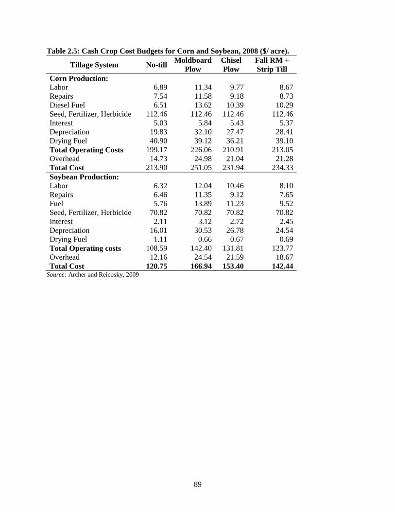
89

Table 2.5: Cash Crop Cost Budgets for Corn and Soybean, 2008 ($/ acre).

Tillage System No-till Moldboard

Plow

Chisel

Plow

Fall RM +

Strip Till

Corn Production:

Labor 6.89 11.34 9.77 8.67

Repairs 7.54 11.58 9.18 8.73

Diesel Fuel 6.51 13.62 10.39 10.29

Seed, Fertilizer, Herbicide 112.46 112.46 112.46 112.46

Interest 5.03 5.84 5.43 5.37

Depreciation 19.83 32.10 27.47 28.41

Drying Fuel 40.90 39.12 36.21 39.10

Total Operating Costs 199.17 226.06 210.91 213.05

Overhead 14.73 24.98 21.04 21.28

Total Cost 213.90 251.05 231.94 234.33

Soybean Production:

Labor 6.32 12.04 10.46 8.10

Repairs 6.46 11.35 9.12 7.65

Fuel 5.76 13.89 11.23 9.52

Seed, Fertilizer, Herbicide 70.82 70.82 70.82 70.82

Interest 2.11 3.12 2.72 2.45

Depreciation 16.01 30.53 26.78 24.54

Drying Fuel 1.11 0.66 0.67 0.69

Total Operating costs 108.59 142.40 131.81 123.77

Overhead 12.16 24.54 21.59 18.67

Total Cost 120.75 166.94 153.40 142.44 Source: Archer and Reicosky, 2009

90

Table 2.6: Biomass Costs for Corn Stover Removal.

Operation COST

Shredding1

10.63 $/acre

Raking2

6.80 $/acre

Baling 12.67 $/acre

Wrapping 4.60 $/ton

Moving 4.57 $/ton

Loading 3.10 $/ton

Storage 7.31 $/ton

Transportation 0.303 $/ton/mile w/in 25 miles of plant

0.198 $/ton/mile 26-100 miles from plant

0.16 $/ton/mile >100 miles from plant Source: Petrolia, 2006 1 Assumed this was done in conventional till (CT) regardless of whether biomass harvested. For Strip Till (ST) it is

assumed this would only be used if raking (>30% harvest) 2 Assumed this would only be used for >30% harvest, otherwise could just bale the windrow.

91

Table 2.7: Comparison of Farm Profits under Different Tillage Practices.

Tillage

System MP1 ST

1 CP

1 NT

1 MP

1 ST

1 CP

1 NT

1

------ Nitrogen Supplement------- --------No Additional Nitrogen ------

% BM

Removed 0.22 0.76 0.80 0.81 0.21 0.76 0.80 0.81

SOC (lb/acre) 0.00 121.62 0.00 84.03 0.00 123.38 0.00 83.32

Corn Profit

($/Acre) 35.04 46.59 44.57 52.24 33.91 45.98 43.98 50.47

Soybean Profit

($/Acre) 77.83 84.32 82.99 95.37 77.83 84.32 82.98 95.37

Biomass Profit

($/Acre) 0.08 2.21 12.30 1.83 2.68 18.06 23.28 18.89

Total Profit 112.96 132.19 139.86 148.53 114.42 148.37 150.25 164.73 1MP: Moldboard Plow, ST: Strip Till, CP: Chisel Plow, NT: No-Till

92

None: Farmer is not responsible for harvesting, loading, transport and storage costs

H: Farmer is responsible only for the harvesting costs

HL: Farmer is responsible for harvesting and loading costs

HLT: Farmer is responsible for harvesting, loading and transport costs

HLTS: Farmer is responsible for harvesting, loading, transport and storage costs

Figure 2.1: Change in Farm Profits with Change in Biomass Prices.

93

None: Farmer is not responsible for harvesting, loading, transport and storage costs

H: Farmer is responsible only for the harvesting costs

HL: Farmer is responsible for harvesting and loading costs

HLT: Farmer is responsible for harvesting, loading and transport costs

HLTS: Farmer is responsible for harvesting, loading, transport and storage costs

Figure 2.2: Change in Farm Profits with Change in Carbon Prices.

94

Figure 2.3: Response Surface of Farm Profit Versus Biomass Price Showing Removal Rate

Contours for a Case Farm Responsible for Harvesting of the Biomass.

Biomass

Removal

Rate

95

Risks and Returns for Cattle Owners under Contract Grazing

I. INTRODUCTION

Traditionally, stocker production has been an integrated operation. Producers

breed calves, wean them and put them on a pasture. Calves graze on the pasture consuming feed

high in roughage (e.g. oats, ryegrass, rye, millet) for 90-180 days. After that they are given a

concentrated feed (e.g. corn) for another 100-200 days based upon their weight till they are ready

for slaughter.

Integrated operations are capital intensive. Johnson et al. (1987) reported the cost

of back-grounding 200 steers on a 100 acre farm on ryegrass would be $50,000 for animal

purchase and an additional $10,000 for forage production. Moreover, the operator has to take

both production risk and price risk. Production risk arises as a result of variability in weight gain

of cattle due to agronomic and climatic factors. Variability exists in both the purchase and selling

prices of cattle due to market forces resulting in a price risk. Cattle prices have always been very

volatile (Spreen and Arnade, 1984). The cattle owner has limited options of reducing price risks

by opting for cattle futures or forward contracting (Harrison et al., 1996)

Since the mid-twentieth century, the use of grazing contracts in cattle production

has become very common in the cattle industry (Anderson et al., 2004). In this case, a pasture

owner does not need to breed or purchase calves and incur heavy investments. Pasture owners

could allow cattle owners to graze their animals on the pasture for a fee, which is usually in the

96

form of a set amount per unit of weight gain. Thus, contract grazing provides a revenue-

generating opportunity for those pasture owners whose cattle purchasing opportunity is limited

due to cash flow concerns (Zaragoza-Ramírez et al., 2008)

With the option to contract graze we define two new categories of operators: a)

pasture owners, who do not own any cattle and allow cattle owners to graze cattle on their

pasture; and b) cattle owners, who own cattle but don‟t own any pasture. The cattle owners

would purchase weaned calves and then contract for the pasture owner to add weight to them.

The term “integrated operator” in this paper refers to an operator who owns both the cattle and

the pasture.

Contract grazing presents an opportunity to the cattle owner to reduce fixed

investment costs. This means low entry and exit costs. Although, being a cattle owner is less

profitable than being an integrated operator (Anderson et al., 2004), it is advantageous in the

form of less capital requirements.

Many previous studies in contract grazing have been forage studies comparing the

risks and returns of a pasture owner to a cattle owner and/or integrated operator. Zaragoza-

Ramírez et al., (2008) have suggested traditional cattle ownership to be more profitable than

contract grazing assuming there are no investment limitations. Johnson et al. (1987) showed that

an integrated cattle owner has larger profits than a non-integrated cattle owner, with only slightly

higher levels of risk; whereas risk for the cattle owner is substantially higher than the pasture

owner. Most studies have shown that contract grazing presents lower risk to the pasture owner as

compared to total ownership under an integrated program (Anderson et al., 2004; Harrison et al.,

1996; Johnson et al., 1987). Little research has compared different strategies for cattle owners in

97

terms of risk and returns. No previous study has examined options available to the cattle owner

to lower risks.

The objective of this paper is to study the factors affecting risk and profitability

for the cattle owner and to assess various options available for reducing risk. Critical decision

factors for the cattle owner include the initial weight at which to buy the cattle, the duration for

which they are kept in the pasture and the duration for which they are kept in the feedlot.

Johnson et al. (1987) have noted that weight gains in pasture vary from year to year whereas they

are predictable in feedlots. As a secondary objective, the paper compares the risks and returns in

an alternative case where the cattle owner bypasses the pasture and places cattle directly at the

feedlots.

II. DATA

This section describes data used in the study.

Pasture data

The data for cattle weight gain on pasture used in this study were collected from

various field experiments (PRN# 2007-118) conducted over four years (2006-2009) at the Beef

Cattle Unit of the Alabama Agricultural Experiment Station‟s E.V. Smith Research Center,

Shorter, AL. For each year, weaned cattle were weighed and randomly placed on different

paddocks on the pasture using a completely randomized design. The cattle grazed continuously

throughout the grazing period and were weighed approximately every 28 days. A total of 854

cattle were studied over four years with an average starting weight of 530 lbs and an average

ending weight of 790 lbs resulting in an average daily gain (ADG) of 2.6 lbs/day. The details of

the forages, stocking rates, grazing days and treatment are shown in table 3.1.

98

Data from different experiments were used to represent one source of risk to the

cattle owner. Under contract grazing, a cattle owner enters into a contract with a pasture owner

to place cattle on pasture and then pays the pasture owner a fixed amount per pound of weight

gain. The contract generally specifies pasture practices such as types of forages fed, stocking

rates, additional feed/supplements given, implants and immunizations given. In reality, however,

in spite of the contract, the pasture owner actually has complete control of pasture practices

(Mcfarland, personal communication, 2009). Forages might vary year to year depending on

choices of the pasture owner. The pasture owner would also control practices such as stocking

rate or feeds/supplements. For example, in the case of a good forage crop, the pasture owner

might skip the supplements or may increase the stocking rate. Similarly, if the crop is poor the

pasture owner might provide additional supplements/implants if the cost of supplements/implants

per pound of weight gain is less than the value of the additional gain.

In sum, although profits of both the pasture owner and cattle owner depend upon

the weight gained by the cattle, only the pasture owner has control of the pasture practices. To

reflect actual risk presented to the cattle owner, the data must be randomly collected over

different years, using different forages with differences in pasture practices such as

feeds/supplements, implants, and immunizations.

Feedlot data

Contrary to pasture practices, a feedlot presents a controlled environment for the

cattle. At the feedlot, cattle are not affected by the amount or quality of forage. Year, weather

and rainfall have little or no effect as cattle are fed a predetermined ration. For the feedlot, the

cattle owner has complete control and can decide what is fed to the cattle. Most feedlots will

provide details on individual cattle basis.

99

The data for the feedlot operations were obtained from the Alabama Pasture to

Rail Program conducted by Alabama Cooperative Extension System (ACES) every year (ACES,

2010). This retained ownership program provides individual post-weaning growth, carcass and

health information to cattle owners. Under this program, cattle owners consign cattle having an

average weight between 600 and 850 lbs. Cattle are weighed, tagged and graded at the shipping

point. The cattle are then sent to Decatur County Feed Yard, Oberlin, KS. Upon arrival, cattle are

fed starter ration and free choice hay. Cattle are managed on an individual basis rather than by

the pen, which means feed and weight gain records of individual animals are maintained.

Depending on the back fat, cattle could be harvested over a two to seven month

period. The cattle are sold upon reaching approximately 0.4 inch back fat. Cattle are sold

individually based upon carcass characteristics to Cargill on a negotiated grid which is based on

yield and quality grade (USDA yield grade 3 calves grading). Premiums and discounts are added

to individual carcass data. The quality grade of cattle is determined by the quality of fat on the

cattle. The variation in quality also presents a risk to the cattle owner.

The data contained starting weights, number of days on feedlot, expenses on feed,

ending weight and selling price of each individual animal. Data for a total of 489 cattle were

collected over three years, 183 cattle for 2006, 86 cattle for 2007 and 220 cattle for 2008. The

average starting weight was 660 lbs. Cattle gained an average of 606 lbs over 182 days resulting

in an ADG of 3.29 lbs/day.

Price Data

Cattle purchase price data for the state of Alabama were obtained from ACES

publications (Prevatt and Todd, 1997; Prevatt et al., 2008). A total of 21 years of data (1986-

1996 and 1998-2007) was used for four weight ranges; 400-500 lbs, 500-600 lbs, 600-700 lbs

100

and 700-800 lbs for medium and large number 1 grade feeder steers. Cattle prices for each

category were adjusted to the 2007 prices using the consumer price index (CPI). Actual

individual selling price data were available from the feedlot for each animal sold.

III. MODEL

A stochastic simulation model using Simulation and Econometrics to Analyze

Risk (SIMETAR) software was used to empirically estimate the return on investment (ROI)

distributions for a cattle owner. SIMETAR is an Excel™ add-in for conducting complex

stochastic simulation models for decision making and risk analysis. The ROI function is given by

the ratio of total profit to total costs.

ROI = π/C (1)

where π is the profit function and C is the cost function.

The profit function (π) is represented by:

π = N* (S – C) (2)

where N represents number of animals. S is the selling price of the animal ($) and is stochastic.

The Cost function (C) is represented by:

C = (CPP*Wt)+TCp+(WGp*CPp)+TCf+(WGf*CF) (3)

where CPP is the stochastic purchase price of a weaned animal ($/lb); Wt is the average weight

of the animal purchased; TCp is the transportation cost to transport the weaned animal to the

pasture ($); WGp is the stochastic weight gained by the animal at the pasture (lbs); CPp is the

contract price ($/lb) for weight gained at the pasture and is varied across a range of prices for the

analysis; TCf is the transportation cost to transport the animal from pasture to feedlot ($); WGf is

the stochastic weight gained by the cattle at the feedlot (lbs) and CF is the stochastic feed cost

per pound of weight gained for the animal at the feedlot ($/lb).

101

An empirical distribution was estimated and used to simulate CPP. Prices for each

weight range were reflected as a ratio to the base weight (400-500lbs). This ensured that each

simulation reflected the decline in prices ($/lb) for heavier animals. Average feed cost (CF) per

pound of weight gained for the animal at the feedlot is also estimated similarly using an

empirical distribution.

Linear regressions were performed to estimate ending weights at the pasture and

feedlot respectively (WGp and WGf) and to ascertain the impact of variables such as starting

weight, and number of days on the ending weight. The estimations of WGp and WGf are

discussed in detail further below in the section named estimated relationships.

The final selling price (S) of the animal is dependent on the quality of fat on the

animals. The fat gained on the feedlot is of higher quality than that from the pasture operations

due of the nature of the feed given to the cattle. To capture this variable into the analysis, a

quality variable was created to reflect the fat gained at the feedlot by taking a ratio of weight

gained on feedlot to the starting weight of the animal. Linear regression was performed to see the

effect of starting weight, quality, year and number of days on feedlot on the selling price. The

estimation is discussed in detail further below in the section named estimated relationships.

Assumptions

For the pasture study, the grazing data were divided into three subgroups to study

different scenarios with starting weights ranging between 400-500 lbs, 500-600 lbs, and 600-700

lbs. Summary statistics for the three weight ranges are presented in table 3.2. It is assumed that

the cattle owner would purchase the cattle within a radius of 300 miles of the pasture. A radius of

300 miles is assumed based on personal communication with a cattle owner in Alabama

(McFarland, personal communication, 2009) and also due to the fact that it would cover most of

102

areas supplying weaned cattle in Alabama, Mississippi, Georgia and Northern Florida.

Transportation costs were obtained from the feedlot data from the pasture to rail program using

actual transport costs for transporting animals from the pasture to feedlot. They were calculated

to be $3.1 per mile for a truck load. A weight loss of 2% during transportation applied to the data

(McFarland, personal communication, 2009). Cattle in the above three categories were grazed

for 100, 95 and 90 days respectively so that the average ending weights will be at approximately

700 lbs, 800 lbs and 900 lbs respectively. These ending weights are realistic, given the starting

weights, and correspond to the typical starting weights at the feedlot and also match the

conditions of the Alabama pasture to rail program.

Feedlot data were divided into six categories. The first three are for the above

mentioned scenarios where the animals are taken from pasture and sent to the feedlot. The

remaining three categories were created for placing the cattle directly onto the feedlot skipping

the pasture. The average starting weights for these categories are approximately 550 lbs, 650 lbs

and 750 lbs. The summary statistics for the feedlot data are in table 3.3.

A contract price of $0.30/lb for the pasture grazing was assumed for the base

scenario keeping in line with the equal return grazing fee5 of $0.3080/lb found by Anderson et al.

(2004).

Estimated Relationships

Linear regression was performed to ascertain how starting weight, number of days

and year affect the ending weight of the animal and to obtain the predicted ending weight for the

cattle while in pasture and feedlot. The relationship between ending weight to starting weight,

number of days and year were assumed to be linear. Since, weight gain at the feedlot is not

5 equal return grazing fee is the fee at which both pasture owner and cattle owner would have equal returns.

103

affected by the weather; year did not have any significant effect on the weight gain and was

excluded from the final regression results. The regression results for the weight gain at pasture

and feedlot are given in table 3.4 and table 3.5, respectively.

Linear regression was performed to see the effect of year, starting weight, quality

and number of days on pasture on the selling price. Although year does not have an effect on the

weight gain, it would affect the selling price due to market cycles. Equation 4 was estimated

using ordinary least squares (figures in parentheses are the estimated standard errors of the

coefficients).

S = -37824.76 + 18.64*Y + 421.81*Q + 1.51*SW + 0.87*D (4)

(11416.18) (5.68) (33.05) (0.07) (0.20)

R2 = 50.8%

where, S is the selling price of the animal, Y is the year, Q is the quality of the

animal, SW is the starting weight of the animal and D is the number of days on feedlot.

IV. RESULTS

The ROI data were simulated with 500 iterations using SIMETAR. Profit/loss and

return on investments (ROI) for all categories described above were calculated and compared for

a batch of 100 cattle. Table 3.6 provides results of the simulation, including ROI. The results

show that buying lighter animals and feeding them in pastures before sending them to feedlot is

the most profitable option. The most profitable option for the base scenario was to purchase the

animals with an average weight of 450 lbs, put them in a pasture for 100 days followed by 220

days on feedlot to earn an average of 7.83% ROI. The ROI for the remaining five categories are

5.47%, 2.44%, 2.42%, 1% and -0.15% respectively as shown in table 3.6.

104

To compare risk for the six scenarios, a stop light chart was created (figure 3.1).

The probabilities of different ranges of ROI are depicted in the stoplight chart. The red shaded

area in each bar represents the probability of a negative ROI. The green area represents the

probability of an ROI>10%. The yellow area would be the probability that the ROI lies between

0% and 10%. The results show that most profitable option in the base scenario above is also the

least risky option. In this scenario, the probability of having an ROI more than 10% is 45% and

the farmer would still incur losses 28% of the times. This also shows that at a contract price of

$0.30 /lb, there is a 28% to 43% chance of incurring a loss any given year depending on the

starting weight of cattle. This is in line with 36% chance of losing money any year found by

Johnson et al. (1987).

The results highlight that at a contract price of $0.30 /lb returns for buying heavier

cattle (600-700lbs) and putting them on pasture before taking them to feedlot are quite

comparable to buying lighter cattle (500-600lbs) and placing them directly on to feedlot. This

shows a possibility that at a higher grazing contract a cattle owner might skip the pasture route

and place cattle directly on to the feedlot. This possibility is studied in detail in the following

subsection.

Effect of Contract Price:

The simulations were re-run with different contract grazing prices, for a case

where cattle are bought at an average starting weight of 550 lbs. We compared the profitability

and risk at five different contract prices ($0.20/lb, $0.30/lb, $0.40/lb, $0.50/lb and $0.60/lb). The

ROI for the contract prices of $0.20, $0.30, $0.40, $0.50 and $0.60 were 7.08%, 4.73%, 2.48%,

0.32% and -1.75% respectively, for cattle that were contract grazed before going to the feedlot.

By contrast, the ROI for going directly to the feedlot was 2.42%. Further sensitivity analysis

105

showed that the “break-even” contract grazing price was $0.41/lb. At prices above this level, it is

more profitable for the cattle owner to place the cattle directly on the feedlot.

The stop light chart (figure 3.2) in this scenario shows that by placing 550 lbs

average weight cattle directly on to the feedlot, the probability of a positive ROI would be 58%

of which 29% would provide more than 10% ROI. In comparison, at a contract price of $0.40/lb

the probability of a positive ROI is 57% although the probability of a ROI more than 10% is 33%

in this case.

Decision to skip pasture:

To further study a cattle owner‟s preferences regarding skipping the pasture and

placing cattle directly on the feedlot, a stochastic dominance analysis was performed. Stochastic

dominance analysis (Hadar and Russell, 1969) is a technique used to compare probability

distributions to study risk efficient action choices. The first and second degree dominance tables

are shown in table 3.7. The second degree dominance table shows that feedlot option is

dominated by 20 cents, 30 cents and 40 cents which suggests that at higher contract prize for

grazing, the cattle owner would be better off by skipping the pasture and placing the animals

directly at the feedlot.

Stochastic efficiency with respect to a function (SERF) is another technique used

to order risky alternatives using their certainty equivalents (CE) for alternative absolute risk

aversion coefficients (ARACs) where CE is the amount accepted in lieu of a higher but uncertain

amount. The stochastic efficiency chart (figure 3.3) also confirms that the feedlot is the 4th

preferred option after the contract rates of 20 cents, 30 cents and 40 cents respectively.

106

V. CONCLUSIONS

The results of the study show that it is always more profitable to buy lighter cattle

than heavier cattle in spite of the fact that lighter cattle command a premium in the market. Also

the probability of positive ROI decreases with the higher starting weights of the cattle. At the

current contract prices, it is more profitable for the cattle owners to send the cattle to pasture

before sending them to feedlot. However an increase in the contract prices might encourage the

cattle owners to skip the pasture altogether and put cattle directly onto the feedlot.

107

VI. REFERENCES

ACES. Alabama Pasture to Rail Program. 2010. Alabama Cooperative Extension Services.

http://www.ag.auburn.edu/ansc/new/extension/AlabamaPasturetoRail.php. Accessed

November 22, 2010.

Anderson, J.D., C. Lacy, C.S. Forrest, and R.D. Little. 2004. “Expected Utility Analysis of

Stocker Cattle Ownership Versus Contract Grazing in the Southeast.” Journal of

Agriculture and Applied Economics. 36:719-730.

Johnson, E., T.H. Spreen, and T. Hewitt. 1987. “A Stochastic Dominance Analysis of Contract

Grazing Feeder Cattle.” Southern Journal of Agricultural Economics 19:11-19.

Hadar, J., and W.R. Russell, 1969. “Rules for Ordering Uncertain Prospects.”American

Economic Review, American Economic Association 59(1):25-34.

Harrison, R.W., B.W. Bobst, F.J. Benson, and L. Meyer. 1996. “Analysis of the Risk

Management Properties of Grazing Contracts Versus Futures and Options Contracts.”

Journal of Agriculture and Applied Economics 28:247-262.

McFarland, Jeff. 2009. Personal Communication, March 12, 2009.

Prevatt, J.W., and M. Todd. 1997. “Alabama Seasonal Beef Price Trends.” Timely Information

Report, DAERS 97-10. Auburn University, June.

108

Prevatt, J.W., D. Gonsoulin, and C. Prevatt. 2008. “U.S. Cattle Cycles and Alabama Seasonal

Cattle Price Trends.” Timely Information Report, DAERS 08-01. Auburn University,

February.

Spreen, T. H., and C. A. Arnade. 1984. “The Use of Forecasts in Decision Making: The Case of

Stocker Cattle in North Florida.” Southern Journal of Agricultural Economics 16:145-50.

Zaragoza-Ramirez, J., D.I. Bransby, and P. A Duffy. 2008. “Economic Returns for Purchased or

Contract-Grazed Stockers on Marshall Annual Ryegrass.” Agronomy Journal 100:1237-

1241.

109

Table 3.1: Experiment Details for Pasture Data (E V Smith Research Center, Shorter, AL)

Year Cattle Forages

Stocking Rates

(head/acre)

Grazing

Days Treatments

2006 185 Marshall Rye Grass 1, 1.2, 1.5, 1.6, 2 78, 82 Implants/No-implants

Gulf Ryegrass Hay/No-Hay

Rye

Oats

2007 228 Marshall Rye Grass 1.2, 1.6, 2, 2.5, 3 113,114 Implants/No-implants

Gulf Ryegrass Till/No-Till

Wheat

MaxQ Fescue

2008 222 Marshall Rye Grass 1.4, 1.5, 2, 2.5, 2.6, 3 112, 113 Implants/No-implants

Gulf Ryegrass Till/No-Till

Wheat

MaxQ Fescue

2009 219 Marshall Rye Grass 1.4, 1.5, 2, 2.5, 2.6, 3 91 Implants/No-implants

Gulf Ryegrass

Marshall Rye Grass +

Wheat

MaxQ Fescue

110

Table 3.2: Summary Statistics for Pasture Data (E V Smith Research Center, Shorter, AL)

(2006-2009)

Weight Range

Number

of

Animals

Average

Starting

Weight (lbs)

Average

Ending

Weight (lbs)

Average

Weight

Gained (lbs)

Average

Days on

Pasture

Average

Daily

Gain

(lbs)

400-500lbs 412 463 717 254 98 2.61

500-600lbs 439 546 807 260 101 2.59

600-700lbs 438 639 919 280 106 2.63

111

Table 3.3: Summary Statistics for the Feedlot Data (Decatur County Feed Yard, Oberlin, KS)

(2006-2008)

Number

of

Animals

Average

Starting

Weight

(lbs)

Average

Ending

Weight

(lbs)

Average

Weight

Gained

(lbs)

Average

Days

on

Feedlot

Average

Daily

Gain

(lbs)

Average

Feed

Cost

($/lb)

Average

Quality

Score1

Average

Selling

Price

($/lb)

Animals from pasture

146 699 1288 591 176 3.29 0.62 0.85 1174.78

76 793 1353 560 171 3.24 0.66 0.71 1232.59

44 890 1425 535 161 3.29 0.76 0.6 1267.44

Animals directly put into Feedlot

136 556 1202 644 191 3.36 0.61 1.16 1077.05

158 649 1248 601 182 3.24 0.61 0.93 1132.57

130 749 1321 574 172 3.28 0.64 0.77 1206.76 1 Calculated as ratio of weight gained in Feedlot to starting weight

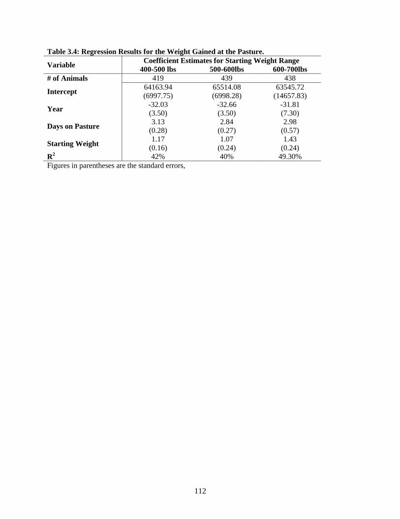
112

Table 3.4: Regression Results for the Weight Gained at the Pasture.

Variable Coefficient Estimates for Starting Weight Range

400-500 lbs 500-600lbs 600-700lbs

# of Animals 419 439 438

Intercept 64163.94 65514.08 63545.72

(6997.75) (6998.28) (14657.83)

Year -32.03 -32.66 -31.81

(3.50) (3.50) (7.30)

Days on Pasture 3.13 2.84 2.98

(0.28) (0.27) (0.57)

Starting Weight 1.17 1.07 1.43

(0.16) (0.24) (0.24)

R2 42% 40% 49.30%

Figures in parentheses are the standard errors,

113

Table 3.5: Regression Results for the Weight Gained at the Feedlot

Dependent

Variable

Pasture and Feedlot Feedlot only

Starting Weight Range

700-800lbs 800-900lbs 900-1000lbs 550-650lbs 650-750lbs 750-850lbs

# of

animals

146 76 44 136 158 130

Intercept 267.42

(191.44)

551.39

(194.8)

764.78

(152.32)

69.02

(172.19)

366.21

(172.43)

771.62

(195.44)

Days on

Pasture

1.61

(0.26)

0.98

(0.29)

0.11

(0.41)

1.74

(0.27)

2.37

(0.23)

1.16

(0.27)

Starting

Weight

1.05

(0.25)

0.80

(0.24)

0.72

(0.14)

1.44

(0.29)

0.70

(0.25)

0.47

(0.24)

R2 24.5 23.5 41.8 31.1 40.7 13.8

114

Table 3.6: Returns on Investment (ROI) for 100 Cattle under Different Starting Weights and

Different Feeding Options

PASTURE AND FEEDLOT FEEDLOT ONLY

Weight Range (lbs) 400-500 500-600 600-700 500-600 600-700 700-800

Animal Purchase

Number of Animals 100.00 100.00 100.00 100.00 100.00 100.00

Purchase Price ($/lb) 1.26 1.14 1.05 1.14 1.05 0.99

Avg. Purchase Weight (lb) 450.00 550.00 650.00 550.00 650.00 750.00

Total Purchase Cost ($) 56,600 62,480 68,406 62,480 68,406 74,412

Pasture Costs

Avg. St. Weight (lb) 441.00 539.00 637.00 NA NA NA

Transport Costs ($) 862.89 1,054.64 1,246.39 NA NA NA

Days on Pasture 100.00 95.00 90.00 NA NA NA

Average Ending Wt (lbs) 708.95 800.54 884.40 NA NA NA

Contract Price ($/lb) 0.30 0.30 0.30 NA NA NA

Contract Payments ($) 8039 7846 7422 NA NA NA

Feedlot Costs

Starting Wt 694.77 784.52 866.71 539.00 637.00 735.00

Transport Costs 5,506.60 6,217.97 6,869.38 4,271.99 5,048.72 5,825.44

Days on Feedlot 220.00 190.00 160.00 220.00 200.00 180.00

Average Ending Wt (lbs) 1,358.53 1,378.86 1,409.23 1,222.47 1,284.68 1,335.79

Feed costs ($/lb) 0.66 0.71 0.80 0.64 0.63 0.67

Quality 0.96 0.76 0.63 1.27 1.02 0.82

Total feed cost ($) 43,643 42,076 43,437 43,810 41,096 40,297

Profit and Loss

Predicted Sale Price ($) 1,226.01 1,251.79 1,294.08 1,122.95 1,147.34 1,193.61

Simulated Sale Price ($) 1,236.24 1,262.24 1,304.89 1,132.32 1,156.92 1,203.58

Total costs ($) 114,651 119,675 127,381 110,562 114,550 120,535

Total Sales ($) 123,624 126,224 130,489 113,232 115,692 120,358

Profits ($) 8,973 6,550 3,108 2,670 1,141 -177

ROI 7.83 5.47 2.44 2.42 1.00 -0.15

115

Table 3.7: Estimates of First and Second Degree Stochastic Dominance

First Degree Dominance (FDD)

20 cents 30 cents 40 cents 50 cents 60 cents Feedlot

20 cents FDD FDD FDD

30 cents FDD

40 cents FDD FDD

50 cents FDD FDD

60 cents FDD

Feedlot FDD FDD

Second Degree Dominance (SDD)

20 cents 30 cents 40 cents 50 cents 60 cents Feedlot

20 cents SDD 30 cents 40 cents 50 cents 60 cents Feedlot

30 cents SDD 40 cents 50 cents 60 cents Feedlot

40 cents SDD 50 cents 60 cents Feedlot

50 cents SDD 60 cents

60 cents SDD

Feedlot SDD 50 cents 60 cents

116

Figure 3.1: Stoplight Chart Comparing Return on Investments under Different Starting

Weights and Feeding Options.

117

Figure 3.2: Stoplight Chart Comparing Return on Investments under Different Contract

Pricing and Feeding Options.

118

Figure 3.3: Stochastic Efficiency With Respect to a Function (SERF) Assuming a Negative

Exponential Utility Function

20 cents

30 cents

40 cents

50 cents

60 cents

Feedlot

ARAC 20 cents 30 cents 40 cents 50 cents 60 cents FeedlotContract Price ($/lb)

Documents

Essays on the Profitability of Winter Farming Enterprises