Embed Size (px)
Citation preview

Clemson UniversityTigerPrints
All Dissertations Dissertations
8-2019
Essays on Two-sided Platforms: Market EntryStrategy and Dynamic PricingQing WeiClemson University, [email protected]
Follow this and additional works at: https://tigerprints.clemson.edu/all_dissertations
This Dissertation is brought to you for free and open access by the Dissertations at TigerPrints. It has been accepted for inclusion in All Dissertations byan authorized administrator of TigerPrints. For more information, please contact [email protected].
Recommended CitationWei, Qing, "Essays on Two-sided Platforms: Market Entry Strategy and Dynamic Pricing" (2019). All Dissertations. 2449.https://tigerprints.clemson.edu/all_dissertations/2449

Essays on Two-sided Platforms: Market EntryStrategy and Dynamic Pricing
A DissertationPresented to
the Graduate School ofClemson University
In Partial Fulfillmentof the Requirements for the Degree
Doctor of PhilosophyEconomics
byQing Wei
August 2019
Accepted by:Dr. Chungsang Tom Lam, Committee Chair
Dr. Matthew S. LewisDr. F. Andrew HanssenDr. James BrannanDr. Scott L. Baier

Abstract
This dissertation consists of two chapters: In the first chapter, we build a the-
oretical framework to study the dynamic entry interactions between two platforms with
homogeneous products into city-based markets. This research is applicable for studying
the entry strategies between, for example, Uber and Lyft; Groupon and Living Social,
and other business models with the attributes of switching cost, network effect, and seg-
regated markets. We address three questions in this paper: 1) What determines the
expansion path of city-based platforms?; 2) What factors are affecting the market con-
centration structures; and 3) Under what conditions can a second mover become the
market leader (with more than 50% of the market share)? We find that a significant de-
gree of the network effect and large switching cost will build a natural barrier for the late
entrant; Transaction-efficient markets with larger transaction volume are less likely to be
concentrated than transaction-inefficient markets. We take consideration of entry cost
and initial fund in our dynamic settings, and find that the uncertainty in market return
will make the platforms’ expansion path and the final outcome less predictable. However,
on average, the capability of capturing the largest market first is crucial for both players;
if a platform loses the opportunity of being the first to capture the largest market, it
may have to raise a considerable amount of money to overcome its disadvantages in the
ii

following competitions.
In the second chapter, we empirically investigate the effect of the dynamic pric-
ing system on ride-sharing platform drivers’ labor supply. Rather than working-hour
and wage-rate relation explored by previous and current literature, we examine the in-
stantaneous response of drivers to price surges. Using data from New York City, we
estimate the structural model through a constrained non-parametric instrumental vari-
able (NPIV) approach. We find that the emergence of a price surge is a strong incentive
for drivers, and the dynamic pricing scheme of ride-sharing platforms effectively solves
the geographical disparity problem of uncoordinated taxi systems. Consequently, the
overall accessibility and quantity of pickup service in the entire city will increase. In the
absence of dynamic pricing, we show in a counterfactual analysis that platform drivers
will be clumped in the Manhattan area and airports, a dilemma shared by the taxi
drivers. The counterfactual context implies that 27 % of the total supply will be lost,
including a significantly large 59% reduction in the non-Manhattan area.
iii

Dedication
To my grandma.
iv

Acknowledgments
I am greatly indebted to my advisor, Tom Chungsang Lam for his advice and
encouragement. I give special thanks to James Brannan as well as to F. Andrew Hanssen,
Matthew Lewis, and Scott Baier for being my committee members. I also thank Patrick
Warren, Charles Thomas, Babur De los Santos, and all other participants in the Clemson
IO workshop for their valuable comments. All errors are mine.
I would love to thank my parents for their constant support, and thanks to Yang
Song for his unconditional love.
v

Contents
Title Page . . . . . . . . . . . . . . . . . . . . . . . . . . . . . . . . . . . . . . i
Abstract . . . . . . . . . . . . . . . . . . . . . . . . . . . . . . . . . . . . . . . ii
Dedication . . . . . . . . . . . . . . . . . . . . . . . . . . . . . . . . . . . . . . iv
Acknowledgments . . . . . . . . . . . . . . . . . . . . . . . . . . . . . . . . . . v
List of Tables . . . . . . . . . . . . . . . . . . . . . . . . . . . . . . . . . . . . viii
List of Figures . . . . . . . . . . . . . . . . . . . . . . . . . . . . . . . . . . . . ix
1 Market Entry Strategies for City-Based Platforms . . . . . . . . . . . . 11.1 Introduction . . . . . . . . . . . . . . . . . . . . . . . . . . . . . . . . . . . 11.2 The General Rules . . . . . . . . . . . . . . . . . . . . . . . . . . . . . . . 91.3 Static Game . . . . . . . . . . . . . . . . . . . . . . . . . . . . . . . . . . . 151.4 Dynamic Game . . . . . . . . . . . . . . . . . . . . . . . . . . . . . . . . . 211.5 Numerical Results . . . . . . . . . . . . . . . . . . . . . . . . . . . . . . . 261.6 Conclusion . . . . . . . . . . . . . . . . . . . . . . . . . . . . . . . . . . . 351.7 Tables and Figures . . . . . . . . . . . . . . . . . . . . . . . . . . . . . . . 37
2 Dynamic pricing solves the urban transportation disparity - Evidencefrom NYC on-demand ride-sharing drivers . . . . . . . . . . . . . . . . 522.1 Introduction . . . . . . . . . . . . . . . . . . . . . . . . . . . . . . . . . . . 522.2 Structural Model . . . . . . . . . . . . . . . . . . . . . . . . . . . . . . . . 572.3 Data . . . . . . . . . . . . . . . . . . . . . . . . . . . . . . . . . . . . . . . 592.4 Empirical Framework . . . . . . . . . . . . . . . . . . . . . . . . . . . . . 612.5 Estimation . . . . . . . . . . . . . . . . . . . . . . . . . . . . . . . . . . . 672.6 Counterfactual . . . . . . . . . . . . . . . . . . . . . . . . . . . . . . . . . 742.7 Conclusion . . . . . . . . . . . . . . . . . . . . . . . . . . . . . . . . . . . 752.8 Tables and Figures . . . . . . . . . . . . . . . . . . . . . . . . . . . . . . . 78
vi

Appendices . . . . . . . . . . . . . . . . . . . . . . . . . . . . . . . . . . . . . 82A Notations for Chapter 1 . . . . . . . . . . . . . . . . . . . . . . . . . . . . 83B Proofs for Chapter 1 . . . . . . . . . . . . . . . . . . . . . . . . . . . . . . 84C Estimation methods comparison for Chapter 2 . . . . . . . . . . . . . . . 85
Bibliography . . . . . . . . . . . . . . . . . . . . . . . . . . . . . . . . . . . . . 89
vii

List of Tables
1.1 Examples of local-based platforms . . . . . . . . . . . . . . . . . . . . . . 21.2 First 13 city launches of Uber & Lyft . . . . . . . . . . . . . . . . . . . . . 61.3 Cities entry time of Uber & Lyft . . . . . . . . . . . . . . . . . . . . . . . 81.4 U.S Top cities by population 2016 (in millions) . . . . . . . . . . . . . . . 91.5 Average returns of sequential equilibriums under different values of K . . . 201.6 Sequential game with imperfect information. . . . . . . . . . . . . . . . . . 371.7 Static game payoff matrix. . . . . . . . . . . . . . . . . . . . . . . . . . . . 381.8 PSNEs under different values of K, α, γ, p of transaction-efficient markets. 391.9 PSNEs under different values of K, α, γ, p, of transaction-inefficient markets. 401.10 Simulation results of dynamic games. . . . . . . . . . . . . . . . . . . . . . 42
2.1 Summary Statistics . . . . . . . . . . . . . . . . . . . . . . . . . . . . . . . 592.2 First-stage Linear Regression . . . . . . . . . . . . . . . . . . . . . . . . . 652.3 Estimation Results of Non-parametric B-spline Knots . . . . . . . . . . . 702.4 OLS Estimation Results of Linear Part . . . . . . . . . . . . . . . . . . . . 722.5 Counterfactual: What if surge pricing is banned? . . . . . . . . . . . . . . 756 Notations . . . . . . . . . . . . . . . . . . . . . . . . . . . . . . . . . . . . 837 Summary statistics of coefficients under different estimation methods . . . 858 Percentage of significant coefficients under different estimation methods . 86
viii

List of Figures
1.1 Uber & Lyft competitive market share by revenue QTD 2016 . . . . . . . 71.2 Market share under different values of γ and p . . . . . . . . . . . . . . . 141.3 PSNEs under different values of αK , γ and K. . . . . . . . . . . . . . . . . 411.4 SPNEs under different values of αK , γ and K. . . . . . . . . . . . . . . . . 431.5 Simulation results under different values of p, (aggregation result of 1000
simulations). . . . . . . . . . . . . . . . . . . . . . . . . . . . . . . . . . . 441.6 Simulation results under different values of p, (one special case). . . . . . 451.7 Simulation results under different values of γ, (aggregation result of 1000
simulations). . . . . . . . . . . . . . . . . . . . . . . . . . . . . . . . . . . 461.8 Simulation results under different values of γ, (one special case). . . . . . 471.9 Simulation results under different initial funds, (aggregation result of 1000
simulations). . . . . . . . . . . . . . . . . . . . . . . . . . . . . . . . . . . 481.10 Simulation results under different initial funds, (one special case). . . . . 491.11 Simulation results under different initial funds, (aggregation result of 1000
simulations) . . . . . . . . . . . . . . . . . . . . . . . . . . . . . . . . . . . 501.12 Simulation results under different initial funds, (one special case). . . . . . 51
2.1 Decision tree of representative driver i . . . . . . . . . . . . . . . . . . . . 572.2 Fitted Nonlinear part: f(p) . . . . . . . . . . . . . . . . . . . . . . . . . . 732.3 Estimated Supply Elasticity . . . . . . . . . . . . . . . . . . . . . . . . . 732.4 Average Local Surge Multiplier & Subway Maps. . . . . . . . . . . . . . . 782.5 Average Local Tips & Average Local Trip Distance. . . . . . . . . . . . . 792.6 Aggregate taxi pickups and drop-offs in June 2016, NYC. . . . . . . . . . 802.7 Real ride-sharing pickups and the counterfactual pickups in June 2016,
NYC. . . . . . . . . . . . . . . . . . . . . . . . . . . . . . . . . . . . . . . 818 Fitted f(p) under different estimation methods . . . . . . . . . . . . . . . 879 Estimated supply elasticity under different estimation methods . . . . . . 88
ix

Chapter 1
Market Entry Strategies for
City-Based Platforms
1.1 Introduction
Today, increasing numbers of businesses are organized around platforms, via
which multiple sides interact to conduct transactions. These companies are involved
in areas such as social media (Facebook), online trading platform (eBay), and search
engine (Google). The majority of these platforms compete in one aggregate market,
and therefore their entry decision has broader boundaries — once an entry decision is
made, soon it will open access to users on all sides; in this way, we will only observe one
entry movement at one specific time. In contrast, some platforms have narrower market
boundaries, such as Groupon, Airbnb, and Uber. These platforms need to make contracts
with customers and suppliers from a local base (Table 1.1 lists several examples of city-
based platforms); hence, their expansion paths are quite different from the previously
1

mentioned platforms, their entry decisions could be more discrete and dynamic, and we
may observe several entries with different timings. In this way, markets’ characteristics
and timing of decisions will have a significant influence on a platform’s final performance.
Table 1.1: Examples of local-based platforms
Platform(s) Market Side 1 Side 2
Uber, Lyft, Juno, Via,Didichuxing
Ride-sharing Drivers Riders
UberEats, Yelp Eat 24,Seamless, Meituan
Food Delivery Restaurants Diners
Groupon, Living Social,Yipit, CoolSavings
Online Deal &Promotion
Merchants Deal-Shoppers
OfO, Mobike, CitiBike Bike-sharing RidersAirbnb Room-sharing Room-
ownersTenants
In this paper, we study the entry decision of homogeneous city-based plat- forms.
We attempt to address the following questions: 1) What determines the expansion path
of city-based platforms? 2) What kind of markets are capable of holding more entrants?
And 3) How can a late entrant take over market leadership? To answer these questions,
we build a theoretical framework for market entry strategies for city-based platforms.
We also extend the framework to two-player games. In these games, we test the relative
importance of multiple factors related to the platform economy:
Network effect and switching cost
Network effect and switching cost are two important research streams studying
business operations via platforms. (e.g., Klemperer (1987), Katz and Shapiro (1994),
Anderson (1998), and Lam (2017)). In multi-sided platforms, we have indirect network
effects: such as the case of Uber: as more riders join the platform, the more attractive
2

it is to drivers; and direct network effects: such as social media (Facebook and Twitter).
For these platforms, network effects act as the "Matthew effect" — “to those who has will
more be given”, a large degree of network effect will make the market highly concentrated.
Further, switching cost determines how difficult it is for a late entrant’s products
to be accepted by customers. For platforms with lower switching costs, customers can
easily home in on multiple platforms, such as Amazon and eBay; for platforms with higher
switching cost, it is difficult for users to practice multi-homing,(e.g., cellphone users —
once a cellphone is purchased, it can only support apps from one operating system; or
video game players — games are incompatible between different consoles). In this paper,
network effect and switching cost mutually control the market share function of plat-
forms. We find that a large network effect and large switching cost will result in market
concentration, and make the second mover disadvantaged in the later competitions.
Transaction efficiency and market uncertainty
We also test the player’s equilibrium behavior under different setups of trans-
action efficiency. We find that higher transaction efficiency will make large cities more
attractive to the second mover, and markets with higher transaction volume are less likely
to be concentrated. In this way, occupying the largest market becomes crucial. For a
second mover to take over market leadership, they either needs sufficient initial funds to
capture the largest market before the first mover does, or the market is particularly open
for a second mover with low network effect and adept at multi-homing.
We also take into consideration market uncertainty in our model—before one
market is being explored, its actual return rate or participation rate is unknown to all.
In this way, the first entrant of the market will have to face the risk of possible low return.
The numerical experiments demonstrate that uncertainty in market return will give the
3

second mover more opportunities to catch up with the first mover in the dynamic game.
Entry cost and initial fund
In a similar manner as for a regular start-up company, in our model, before
players start to explore the markets, they will raise an initial fund. We simplified the
fund-raising process to be only one round for both players. Because we don’t allow for
negative market return in our simulations, the players will spend the initial fund on entry
cost. Hence, in each period, a player will make entry decisions by solving a BLP (binary
linear programming) problem. We find that a second mover with a higher initial fund is
more likely to take over market leadership.
1.1.1 Related Literature and Contributions
This paper contributes to the current literature by being the first to construct a
theoretical framework to model the real-world entry dynamics between platforms. The
research applies to businesses with the attributes of network effect, switching cost, market
return uncertainty, and limited market boundaries. We provide adjustable parameters
to fit in different types of platforms.
This work mainly complements the literature studying the order-of-entry prob-
lem (e.g., Lambkin 1988; Mitchell 1989; Lilien and Yoon 1990; Mitchell 1991; Golder
and Tellis 1993; Lee 2008; Wu 2013, etc.). Lieberman has a series of research works
on the first mover advantages, such as Lieberman and Montgomery (1988, 1998) and
Lieberman (2005), Lieberman and Montgomery (1988) survey the theoretical model and
empirical evidence that confer the first mover advantages; they also examine the possi-
ble source of first mover disadvantages. Lieberman (2005) assesses the magnitude and
sources of first-mover advantages in 46 Internet markets; he finds that network effect
4

and patented innovations are related to higher market valuation for pioneer movers. and
Lambkin (1988) find that pioneer incumbents on average outperform late entrants. Pre-
vious works mostly focus on empirically and theoretically identifying the sources of first
mover advantages, whereas in this paper, we apply the concept of first mover advantages
in our model, and ask under what condition can a second mover be able to overcome the
first mover advantages.
Some of the related works on platform entry problems are concluded as follows:
Zhu and Iansiti (2012) build a theoretical model and find that an entrant’s success de-
pends on the strength of indirect network effects and on the consumer expectation of
future applications. They find that under certain conditions, a small quality advan-
tage can help the entrant compete against install-based advantaged incumbent. They
empirically examine the model applicability by investigating the video game industry.
Dewenter, Rösch, et al. (2012) analyze the impact of indirect network effects in emerging
two-sided markets on price, quantities, profits, and market entry, and find that, when
network effect is strong, market entry will no longer occur, thus leading to a natural
monopoly. Seamans and Zhu (2013) empirically investigate the impact of Craigslist’s
entry on local newspapers; and Kim, Lee, and Park (2013) empirically study the two-
sided market entry strategies in the online daily deals promotion industry. Our paper
is different from the above works in two ways: first, we do not focus on post-entry firm
interactions such as pricing strategies or quality competition, but rather we focus on the
decision of entering the market; second, their analyses are mostly within one market,
whereas we are examining the entry decisions into multiple markets.
Although, there have been substantial increases in the literature studying multi-
sided markets (e.g., Armstrong 2006; Rochet and Tirole 2003, 2006; Rysman 2009; Jullien
2011.), most of the theoretical work focuses on optimal pricing strategies and interactions
5

between sides. This work complements this theoretical stream by offering a dynamic
approach to study the interaction between firms.
1.1.2 Motivation
Although the model in this research applies to many local-based platforms, the
motivation of starting this research comes from several interesting unexplained observa-
tions of the leading ride-sharing platforms, Uber and Lyft. First, both Uber and Lyft
have a strong preference for large cities. Uber made its first entry into San Francisco
in 2010; then New York, Seattle, and Chicago in 2011; and San Diego, Los Angeles,
Philadelphia, Atlanta, and so on, in 2012. Two years later, Lyft also launched its first
ride in San Francisco, then Los Angeles, Seattle, Chicago, and so on. If we examine the
first several entries of both platforms (Table 1.2), we can find that both of them have a
strong preference for large cities.
Table 1.2: First 13 city launches of Uber & Lyft
Uber Cities Uber Launch Date Lyft Cities Lyft Launch Date
San Francisco 7/10/2010 San Francisco 6/1/2012New York 5/3/2011 Los Angeles 1/31/2013Seattle 7/25/2011 Seattle 4/1/2013Chicago 9/22/2011 Chicago 5/9/2013San Diego 1/6/2012 Boston 5/31/2013Los Angeles 3/8/2012 San Diego 7/2/2013Philadelphia 6/6/2012 Washington 8/9/2013
Atlanta 8/24/2012 Atlanta 8/29/2013Denver 9/5/2012 Minneapolis/St.Paul 8/29/2013Dallas 9/14/2012 Indianapolis 8/29/2013Boston 9/19/2012 Phoenix 9/5/2013
Minneapolis/St.Paul 10/25/2012 Charlotte 9/12/2013Phoenix 11/15/2012 Denver 9/19/2013
Things can be easily understood for Uber because a large city means a large
market. But if we look at Lyft’s entry path, we notice that Lyft seems to follow the same
entry path as Uber: in the beginning, Lyft always chose to enter the markets already
6

being occupied by Uber, rather than exploring a new but smaller market. More evidence
can be found from the launch choices of other ride-sharing platforms, such as Juno and
Via, who both started in New York; similarly, SitBaq and Summon both started in
San Francisco and the Bay area. Thus the following question arises: Why do second
mover ride-sharing platforms always choose to enter these large cities to face intensive
competition, rather than exploring a new but smaller market?
Second, no matter the entry order and initial funds, Uber always tends to dom-
inate the market. Before Uber started its first launch in San Francisco in 2010, it raised
$1.3M in the angel round. Almost two years later, June 1st, 2012, Lyft, a ride-sharing
platform providing almost an identical service, announced its first launch in the same
city, San Francisco; and this time, with Uber already proving the potential of ride-sharing
business, Lyft raised $7.3M for its debut launch. However, a more successful initial fund-
raising round did not help Lyft become the market leader. Figure 1.1 is a report of Uber
and Lyft’s market share in major cities in 2016 (Peltier 2016).
Figure 1.1: Uber & Lyft competitive market share by revenue QTD 2016
7

We can see from the figure that market shares of both firms are around the ratio
of 20:80, although most of the cites where Uber makes the first entry, there are also
several special cases (Table 1.3).
Table 1.3: Cities entry time of Uber & Lyft
Cities Uber Launch Date Lyft Launch Date
Washington D.C 8/8/2013 8/8/2013
Houston 2/21/2014 2/19/2014
Miami 6/4/2014 5/23/2014
Austin 6/3/2014 5/29/2014
For these four cities, Uber and Lyft entered at almost the same time; for Miami
and Austin, Lyft even entered several days ahead. But we can see from Figure 1.1 that,
Lyft only owned around 16% to 17% of the market; for Houston, it was exceptionally
low, only 3%. Why is the market share ratio so constant across the country, and why
does Uber always dominate the market even when Lyft was the first mover?
This research could also join the recent emerging studies on ride-sharing plat-
forms (e.g. Li, Hong, and Zhang 2016; Hall, Horton, and Knoepfle 2017; Hall and
Krueger 2018; Cramer and Krueger 2016; Greenwood and Wattal 2015; Chen, Mislove,
and Wilson 2015).
The rest of the paper is arranged as follows: In section 2, we will propose the
fundamental model setups applied in later chapters; then, in section 3, we solve for Nash-
equilibriums in static games under different market conditions. In section 4, we extend
the static game to a dynamic game and provide numerical experiments in section 5.
Finally, in section 6, we will state our conclusions and discuss future research potentials.
8

1.2 The General Rules
Before exploring the static game, we will go through three fundamental rules,
which will be applied in the static game and dynamic game, taking account of market
size, pre-entry uncertainty, and the market-splitting rule. These rules will build a general
model framework for the city-based platform entry problem.
Transaction Volume
Suppose each city is a market, and platforms face a line of potential cities ranked
by population size. As in Table 1.4, the largest city in the U.S is New York City; its
population is approximate twice the population of the second largest city, Los Angeles;
and the third largest city Chicago, is nearly one-third the population of NYC, and so on.
This phenomenon (rule) is called "Zipf’s Law for Cities" (Zipf et al. 1949; Xavier 1999).
Table 1.4: U.S Top cities by population 2016 (in millions)
Rank 1 2 3 4 5 6
City New York Los Angeles Chicago Houston Phoenix PhiladelphiaPopulation 8.538 3.976 2.705 2.33 1.615 1.568
Ratio to NYC 100.0% 46.6% 31.7% 27.3% 18.9% 18.4%1 ≈ 1
2≈ 1
3≈ 1
4≈ 1
5≈ 1
6
Data Source: US Census Bureau
Also, suppose platforms compete over a fixed size of the population in each
city, the market rank K has NK service consumer and M
K service provider on each side.
Consider a transaction efficient setup, that every service provider is capable of interacting
with every service consumer. The potential transaction volume of such platforms will be
similar to the setup in traditional two-sided market literature (Rochet and Tirole 2003):
simply multiply both supply and demand sides together, which is equal to NMK2 . From
this setup, the market potential transaction volume is substantially enlarged in large
9

cities. For instance, the first largest market is 4 times the second largest market and 9
times the third ( NM1 compares with NM
4 and NM9 ).
Pre-entry Market Uncertainty
Before being explored, the average benefit αk of each potential transaction in the
Kth market is unobservable to both platforms. However, platforms know the distribution
of the benefit αK ∼ F (αK). Once market K is being explored, αK would reveal to all.
One can consider this αK as a platform-specific city (exogenous) characteristic; because,
for different types of businesses such as Groupon for deals, Airbnb for room-sharing, and
Uber for ride-sharing, αK should have different values. Here, αK has two meanings: first,
it is the platforms’ average profit per potential transaction, which means it takes into
account the revenue and cost at the same time. Second, it also represents the utilization
rate of a platform in the Kth market, because NMK2 is the ideal transaction volume, in
reality, based on city culture and city characteristics, some cities may use the platform
more frequently, and other cities may not use the platform much at all. Hence, αK also
measures each city’s preference.
Market Share
Suppose users in one representative market i are facing a nested choice problem,
and there is no outside option available within this choice set. Before the second mover
enters the market, the incumbent gains all the market share, because no other choice is
available. And after the entry of the second mover, the utility of an average user choosing
10

platform n in one transaction will be:
Unit =
Vnit + γxnt , if platform n is the incumbent
Vnit + γxnt − hn , if platform n is the entrant(1.1)
xnt =mnt
mnt +m−nt
(1.2)
Where γ ∈ [0,∞) represents the parameter of network effect larger γ means
larger network effect, mnt, m−nt are platform sizes of the player and it’s opponent,
calculated by the numbers of users already captured by a platform; xnt is the relative
firm size; Vnit is the average user utility gains from service provided by platform n; it
is related to service price, service quality and other platform characteristics. Finally,
parameter hn represents the dis-utility of switching from incumbent platform −n to
entrant platform n, if n is a second mover.
The market share of each platform based on nested logit choice model is:
Snit =
e(Vnit+γxnt)
e(Vnit+γxnt) + e(V−nit+γx−nt−h−n), if platform n is the incumbent
e(Vnit+γxnt−hn)
e(V−nit+γx−nt) + e(Vnit+γxnt−hn), if platform n is the entrant
(1.3)
If we consider a homogeneous case, that switching cost and average service utility
are the same for both platforms, so that hn = h−n = h and Vnit = V−nit = V , the share
11

functions will become:
Snit =
(exnt)γ
(exnt)γ + p(ex−nt)γ, if platform n is the incumbent
p(exnt)γ
(ex−nt)γ + p(exnt)γ, if platform n is the entrant
(1.4)
Where p = e−h ∈ (0, 1]1, when h = 0, p = e−h = 1, there is no switching cost;
when h→∞, p = limh→∞
e−h = 0, the switching cost of a new platform is extremely large,
users are fully unacceptable for a second mover.
Therefore, the final rule of market share is concluded as follows: When a platform
n decides to enter a new market without any incumbent, it will capture the entire market;
when a platform n decides to enter a market already occupied by another incumbent −n,
they will split the market:
Snit =
1, if market i has 0 incumbent
p(exnt)γ
(exnt)γ + p(ex−nt)γ, if market i has 1 incumbent
(1.5)
S−nit = 1− Snit (1.6)
Therefore, if there are two firms in the market, they will split the market based on
their current firm sizes, parameter p ∈ (0, 1], and parameter γ ∈ [0,∞]. Note here, that,
we essentially assume that platforms are open to multi-homing, but with some degree of
1Note that their could be the case of second mover advantage p > 1, but it is beyond the discussionof this paper. In this paper, we regard the second mover advantage as ahead of disclosure of hiddenmarket information, or the chance of avoiding a bad return market
12

difficulties, parameter p basically is a measurement of second mover disadvantage; but in
the utility function, it is the switching cost per transaction from one platform to another.
One can consider this switching cost has many sources, for example, the monetary cost
induced by the platforms, that users have to pay some amount of money or lose the
opportunity of earning some amount of benefit by switching to a new platform. Another
example is adaption cost: users who are used to one platform will incur some dis-utility
when switching to another one. Typically, researchers mostly consider firms offering
heterogeneous products to have larger second mover disadvantages towards each other.
However, platforms providing similar goods can also establish a barrier to preventing
customers from switching to each other. For example, Lyft and Uber offer power-drive
bonuses for drivers in some cities. If a driver completes a certain number of rides within
a specific period of time, the platform will pay them an extra bonus as a reward. This
method on the one hand keeps the driver active during rush hours; on the other hand,
it creates an opportunity cost, which helps to make the drivers stick to the platforms to
earn the bonus. Another example is cellular service companies — usually, the customer
has to pay a cancellation fee if they want to switch to another service provider, and the
service of the two companies could be highly similar.
This market splitting rule ensures that new entrants with zero market size will
still gain some market share as a second mover, and provides a testable structure for
different types of business models. Both γ and p are treated as exogenous parameters
related only to the type of business, which means in this research that, we will mainly
discuss the case of homogeneous service platforms.
Consider a special case similar to the situation that the first mover has already
been in the market for some time and gained some users, and hence it has some degree
of network effect scaled by γ. Then, the second mover just completes its seed round and
13

starts to explore the markets. For the markets already occupied by the first mover, they
will split the market following the rule in Equations 1.5 and 1.6. For example, refer to
Figure 1.2a when γ = 2 and p = 0.25, the first mover will win 96.7% of the market and
the second mover will only receive 3.3%. Another scenario is described as when a small
firm occupies a market first, then a big company enters the market as a second mover
(refer to Figure 1.2b), where, as long as the network effect γ is not particularly large, an
incumbent can still hold most of its current market even if it is facing a market giant.
(a) Second mover with m2 = 0
(b) First mover with small size m1
Figure 1.2: Market share under different values of γ and p
14

1.3 Static Game
In this section, we will illustrate the above settings more clearly in a two-player
static game, and will also calculate the platforms’ Nash-equilibriums under different
market conditions.
First, we will make the following basic assumptions to build the static game 1)
Firms are risk-neutral2; 2) A firm’s average benefit from each potential transaction is
drawn from one same distribution, i.e., the expectation of profit per potential transaction
is the same for all markets: E(αi) = α ∀i ∈ F , F is the set that includes all feasible
markets 3) Once a market is being explored by a player, it will generate profits in every
subsequent period; 4) p = 1 no switching cost3, and 5) For simplicity, we only consider
three available markets in our model that F := {K,K + 1,K + 2}
Game Setups 1 ( Static Game)
1. Time 1, First mover, Player 1 with size m11 = 0 enters market K reveals market
K’s profit parameter αk, and gain a profit NMK2 αk, update m12 = NM
K2 αk;
2. Time 2, Second mover. Player 2 with size m22 = 0 comes into existence and both
firms simultaneously decide which market to enter.
(a) Player 1 gains profits from market K;
(b) If player 2 decides to enter market K, they will split the market based on their
current relative size m11, m21, and γ, refer to Equation 1.7;
2This assumption is made to simplify the problem; the firms are not necessarily risk-neutral, but afirm’s preference on risks is beyond the discussion of this paper.
3The purpose of inducing the measurement of switching cost, is to make both players have somedegree of disadvantages when acting as a second mover, because in the static game, only Player 2 hasa chance to become second mover; network effect from period 0 will already make them disadvantagedwhen competing in the same market with Player 1. Thus, here p = 1 for simplicity
15

The payoff matrix of this static game can be seen in Table 1.7, where S1 means
the market share of Player 1 as first mover; 1 − S1 means the market share of Player 2
as second mover.
S1 =(e1)γ
(e1)γ + (e0)γ(1.7)
1.3.1 Static Equilibriums
Proposition 1 When Player 2 chooses action K, Player 1 will always choose K+1; when
Player 2 chooses action K+2, Player 1 will always choose K+1; when Player 2 chooses
K+1, if and only if K < 2√S1−1
1−√S1
Player 1 will choose K+1, otherwise Player1 will choose
K+2.
Proposition 2 When Player 1 chooses action K+1, Player 2 will choose K, K+1 or
K+2; when Player 1 chooses action K+2, Player 2 will choose K, K+1 or K+2.
Proposition 3 Four PSNE (pure strategy Nash equilibrium) and two MSNE (mixed
strategy Nash equilibrium) exist in the myopia static game. They are PSNE (K+1,K),
(K+1,K+1), (K+1,K+2), (K+2,K+1); and MSNE in anti-coordination game, (K+1,K+2)
and (K+2,K+1), (K+1,K) and (K+2,K+1)
From proposition 1,2,3, we can see that for each pair of {αK , γ}, there exist a
threshold K for K ∈ Z+, below which ∀K < K, Player 2 will choose to compete; above
which ∀K > K, Player 2 will choose to avoid direct competition. Intuitively, when players
discover that market K is good, Player 2 will be more likely to enter a good market in
period 1. Similarly, when the market condition is welcoming for a second mover, that
both the network effect and switching cost is lower, Player 2 will be more likely to face
competition from Player 1. When K increases, the benefit from market size cannot cover
the loss in competition; both players will tend to explore a new market, rather than
16

compete in an old one. Hence, in this manner, one can expect the benefit of market size
from a transaction-efficient market to be held longer than a transaction-inefficient setup,
because the transaction volume is enlarged in the former one.
Figure 1.3 compares the evolution of PSNEs under transaction-efficient setup
versus transaction-inefficient setups under different values of γ, K, and αK . We can
see that PSNE (K+1, K+1) rarely occurs — only when αK is really below expectation
(αK = 0.1), and the network effect of existing markets is significantly low (γ < 0.3),
most of the time, a later entrant will either enter and compete in the largest city (K) or
explore a much smaller one (K+2).
From Figure 1.3 we can clearly observe the evolution of threshold K with αK
and γ: When αK increases, the margin for Player 1 to deviate to K+2 does not move,
because from Proposition 1, we know that this line is only related to the size of market
share — or at root related to γ; however, the area of PSNE (K+1,K) becomes larger when
αK increases. If we take one horizontal slice of Figure 1.3 to examine the comparative
statics, for example, in the αK = 1.0 high transaction volume scenario, if we hold γ = 2,
and look at the change of different Nash equilibriums under different K, we will be able
to gain some insight in the firm’s entry path. When markets are large, the second mover
will always enter and compete in those larger markets; then, with the decrease of market
size, both firm will finally deviate to a non-aggressive strategy to avoid competition.
The same idea applies if we take a vertical slice from the figure, so that to
hold market size constant and analyze how network effect affects a firm’s entry behavior;
clearly, larger network effect will make second mover more disadvantaged when competing
with the first mover.
Next, in Table 1.8 and Table 1.9, we list several specific numerical experiments
under transaction-efficient markets versus transaction-inefficient markets respectively,
17

with E(αi) = 0.5 and NM equals some arbitrary positive 4 , to further illustrate the
firm’s behavior.
D1, D2 here represent Player 1 and Player 2’s entry decisions, respectively. Mar-
ket share of each firm is controlled by γ. From Tables 1.8 and 1.9 we can see how much
the second mover favors the largest city in transaction-efficient market — whenK = 1, as
long as the market yield is average level or above, the second mover in a platform-based
market will always choose to enter the largest city (see cases 1 to 6). When conditions in
the first market K are not good, αk = 0.1 is quite below the expectation value; player 2
has the advantage of information disclosure, it has the opportunity to avoid the bad ones,
therefore, it will enter market K+1, and K+2, and skip market K. In other scenarios,
when K is larger, and city size is smaller, good profit and welcoming market environment
can still be a strong incentive for Player 2 to enter a competitive market. However, in
most of the cases when the benefit from a large market cannot cover players’ loss from
competition, player 2 will skip the second largest market and jump to the third to avoid
direct competition with Player 1, because even without second mover disadvantages, the
lack in existing network effect will still put it in an unfavorable competing position.
In contrast, the situation for Player 1 will be more favorable — holding the
largest market K in hand, the network effect will give the player many advantages in
the further competitions. Thus, when the market size is large enough, the dominant
strategy for the first mover will always be continuing the previous exploration step to
the next largest city, no matter the strategy of Player 2; when market size is not large
enough (e.g. K = 10 ) or the market does not have large network effects (e.g. γ = 0,
p = 1), there will be two MSNEs: two platforms will play anti-coordination games to
avoid face-to-face competition.
4In static game, the value of NM does not matter to the final Nash-equilibrium, because (refer toTable 1.7) NM will be cancelled from the nominators due to it appearing in all equations
18

An interesting scenario is described in cases 4 to 6, when αk = E(α) = 0.5; one
can regard these cases as: how would a risk-neutral second mover behave if the former
incumbent does not reveal the market information.
1.3.2 Sequential Equilibriums
So far, we have discussed the static equilibriums under one-period static game,
and the static game is based on the assumption that Player 1 does not foresee the advent
of another competitor (or the discount rate is very large). In this subsection, we will
briefly discuss the sequential game under the assumption that Player 1 does foresee the
advent of Player 2’s entry (or there is no discount rate). The game setup is similar:
Game Setups 2 (Sequential Game)
1. Time 1, Player 1 with size m11 = 0, chooses one among market K, K+1 and K+2
to enter, reveal the market information, gain a profit, and update m12
2. Time 2, Second mover. Player 2 with size m22 = 0 comes into existence and both
firms simultaneously decide which market to enter.
The extensive game tree and payoff matrix of each node can be seen in Table 1.6,
because before the first player enters the first market, no market information is known
by either player, Player 1 will guess the state in the second period through expectation
return E(α), and hence E(α) will be cancelled from the payoff matrix. The subgame
perfect Nash equilibrium is solved through backward induction in Figure 1.4, αi here is
the revealed market return after Player 1’s first entry, i here could be K, K+1 or K+2.
In most of the cases, in the beginning period, Player 1 will choose the largest
market K, under several scenarios, Player 1 will choose market K+1 or K+2; note here,
19

if Player 1 does not enter market K in the beginning, market K will be a dominant
strategy in the second period for Player 1 in the subgame, indicating that in the real
world, if the degree of network effect γ is uniformly distributed, most of the time, we
will observe entries into the largest market. Or, in another perspective, if the degree of
network effect is uncertain but follows a uniform distribution, for a start-up platform,
entering the largest market is the safest strategy, because it has the highest probability to
be the best choice. In Table 1.5, we summarize the average return of all tested numerical
experiments of different values of K. Clearly, on average, entering the larger market will
generate better returns.
Table 1.5: Average returns of sequential equilibriums under different values of K
K 1 2 3 5 10
P1 P2 P1 P2 P1 P2 P1 P2 P1 P2
t1
K 0.917 0.142 0.263 0.042 0.122 0.025 0.049 0.011 0.012 0.004K+1 0.679 0.128 0.221 0.059 0.111 0.037 0.044 0.019 0.012 0.006K+2 0.600 0.125 0.181 0.056 0.086 0.032
20

The static game gives us good insights to explain the following phenomenon:
Why in the beginning do second movers such as Lyft, Juno and Gett, always prefer to be
a follower, entering large cities and facing intense competition rather than exploring a new
but smaller market. The nature of platform-based multi-sided interactions significantly
enlarges the amount of transactions in large cities, offsetting the disadvantage as a second
mover and small network effect. On the contrary, the market structure in a non-platform-
based or lower transaction efficiency market would be more concentrated, and we would
expect to see more natural monopolies in such markets.
Static game plots general equilibrium in a simple scenario; there are some caveats
to serve the purpose of mimicking the real world, for example, firms can only enter one
market at a time, the interactions take only one period, and they do not take entry cost
into consideration. In this way, the static setup could not provide answers when the
firms’ interactions are more dynamic or when there are more markets available.
Thus, next, we will present a model of a dynamic sequential game to solve the
above problems and answer the remaining questions.
1.4 Dynamic Game
The fundamental assumptions of the dynamic game are inherited from the pre-
vious static game: 1) Firms are risk-neutral; 2) All markets’ average transaction profits
are drawn from one same distribution: E(αi) = α, ∀i ∈ F , F is the set that includes all
feasible markets. 3) Once a market is being explored by a player, it will generate profits
in every period. Besides the assumptions from the static game, in the dynamic game we
add two more assumptions: 4) The one-time fixed entry cost is diminishing in market
size: cK , for the Kth market, and for both players. Finally, without loss of generality 5)
21

Players move in turn: player 1 moves the even turn, player 2 moves the odd turn;
The structure of entry cost plays a crucial role in designing the algorithm that
solves the firm’s best behavior. Note that, K to the power 1 in the denominator :CK ,
guarantees that the size of the feasible markets set F converges to an upper limit K5:
K = NMrc E(αk) (1.8)
Where the expected present discount value NMrK2E(αK) of the last market K will
just cover the one-time entry cost for the last market cK.
Inducing the entry cost term in the dynamic game is important because, in
the model, it adds a budget constraint for every decision; hence we have a constrained
optimization problem6 to solve; And in reality, a firm’s expansion is closely related to
its money stock; it is rare that a city-based platform would enter all the markets at one
time. As in the ride-sharing case, a platform’s expansion decision is closely related to its
funding rounds. Part of the expansion cost is reflected here as a one-time fixed cost, and
part of the expansion cost is reflected in the post-entry realization of αK as average cost
per potential transaction.
Game Setups 3 (Dynamic Game)
1. Before the game begins, p, γ, r7, are predetermined parameters for both players;
2. Game starts at time 0, t ∈ [0, T ], Xn0 = ∅ for n = 1, 2 , I0 = ∅, J0 = F 8;
3. Player 1 starts at time 0 with initial fund u10; Player 2 starts at time 1 with initial
5Note that here K is different from what it is in static games.6In each period the problem can be simplified to a 0-1 package problem7Parameter r is the discount rate.8It, Jt represent the sets of markets with 1 player, and markets with 0 players respectively. Xnt is
the set of current markets entered by player n at time t
22

fund u21; unt here represents how much money the player n owns at time t;
4. Within each turn, one player will first load the status of its current state.
(a) Load the current states: unt, u−nt, mnt9, m−nt, It, Jt ,Xnt, X−nt;
(b) Calculate Snit and 1 − Snit for i ∈ It ∪ Jt (Equation 1.5 and 1.6) for both
players;
5. Second, a player solves the following binary linear programming (BLP) problem to
find the optimal market entry strategy set (z∗t , y∗tz∗t , y∗tz∗t , y∗t ):
maxyit,zjt
∑i
yitNM
(Ki)2SnitαKi +
∑j
zjtNM
(Kj)2E(α)
s.t. Cnt =∑i
yitcKi
+∑j
zjtcKj≤ unt,
yitcKi≤ NM
r(Ki)2SnitαKi,∀ i ∈ It,
zitcKj≤ NM
r(Kj)2E(α),∀ j ∈ Jt,
yit ∈ {0, 1},∀ i ∈ It,
zjt ∈ {0, 1},∀ j ∈ Jt.
(a) It represents the set of markets already being explored by the other player at
time t, therefore, αKi is revealed to all; Jt represents the set of undeveloped
markets at time t, and hence αKj is not revealed, and players can only make
decisions through expected profit E(α);
(b) Total cost of the entry has to be no larger than a player’s current money stock;
9In this game it equals the amount of revenue one platform generated from the previous t−1 period:Rnt−1.
23

(c) The real present discounted value of a market must cover the entry cost for
markets in It; the expected present discounted value of a market must cover
the entry cost for markets in Jt;
(d) yit and zjt are decision variables of market entry; it is either 1 or 0 (enter or
not);
(e) Snit represents the player n’s market share in market i at time t, when player
n is a first mover Snit = 1
6. Third, update the status for the next period and next player;
(a)
mnt+1 = Rnt =∑i
NM(Ki)2
SnitαKi,∀i ∈ Xnt+1
m−nt+1 = R−nt =∑j
NM(Kj)2S−njtαKj ,∀j ∈ X−nt+1
(1.9)
(b)
unt+1 = unt +Rnt − Cnt
u−nt+1 = u−nt +R−nt − 0
(1.10)
(c)
Xnt+1 = Xnt ∪ y∗ty∗ty∗t ∪ z∗tz
∗tz∗t
X−nt+1 = X−nt
It+1 = It \ y∗ty∗ty∗t ∪ z∗tz
∗tz∗t ,
Jt+1 = Jt \ z∗tz∗tz∗t
(1.11)
7. Repeat Step 4,5,6;
8. If t = T end the game.
24

The basic idea behind this setup is that in a dynamic sequential game, each
player’s action will change the future states for both players, thus, in each period, players
are making decisions upon changing states.
First, note here that mnt and unt are two completely different things. Only by
occupying (some of) the markets can one player make changes in its firm size; mnt here,
is in control of the player’s market share when it has to split the market with the other
one. unt is the platform’s current cash flow, and can be regarded as the aggregation of
that platform’s revenues and costs from time 0 to time t; unt, here, is in control of the
player’s budget constraint of new entries.
Second, we can see from the above game setups that, a player’s market share
is not related to the current market’s characteristics, but is only related to the players’
current state.
Third, once a game is initiated, no intervention is required in the process of
playing. The source of randomness comes from the realization of αK , once the α is known
to all, the "optimal solution" is somehow destined, for one bundle of parameters; as long
as αK are generated for each city, there will only exist one entry path for both players,
although, from the firms’ perspective, they are facing many uncertainties. While, in this
research, we only discuss the situation when αK is positive, with all markets generating
positive returns in each period, and hence there is no need for exit after entry. While if
we allow for negative market return, the post-entry market information disclosure, will
add more randomness to players’ market positions — the late entrant has the chance
to avoid the harmful markets, and therefore could have more opportunity to take the
leadership. Moreover, if both platforms can gradually learn the properties of αK during
the entry process, they may have more chance to survive.
Finally in Step 8, we can see that, the game does not stop at the exact time
25

when It = Jt = ∅ such that no further empty markets are available. This is because,
even after all the feasible markets have been explored, the firms will continue operating.
One can see from the simulation results that, the status of two players will tend to a
steady state after they complete the entry process.
The complexity of the dynamic model makes it difficult to solve for the analytical
solution, hence, in the next section, we will present the results of several numerical
experiments with different initial parameters to gain insights into city-based platforms’
behavior patterns in the market entry problem.
1.5 Numerical Results
In this section, we will describe the numerical experiments, which focus on two
parts: First, we investigate the joint effect of switching cost and network effect on plat-
forms’ market entry decisions. Second, we test the results under different initial funds10.
1.5.1 Network Effect and Switching Cost
From previous setups, we know that, γ and p jointly determine how players split
the market — in homogeneous cases, these two are exogenous parameters related only
to the type of platform’s business model. From static games we know that γ and p
eventually affect the platforms’ willingness to compete. However, one has to note that,
although γ and p control the market share together, p has a more sophisticated effect,
because in a segregate markets setup, if the second player takes the advantage of entering
first, it will be difficult for the first player to enter the market either. The initiation of
10The code for the games and simulations applied in this paper can be found in https://github.com/QingWei2018/two_sided_market_entry_simulation, we use Pyomo to solve for the BLP problems ineach period (Hart, Watson, and Woodruff 2011; Hart et al. 2017).
26

dynamic games in this section will be set as follows:
1. Game starts with K=1, t=0;
2. u10 = 20 , u21 = 20, c = 20, NM = 20 , r = 0.01 ;
3. αKi for i = 1, 2, 3... are generated from uniform distribution U(0, 1), E(αKi) = 0.5;
4. The maximum number of periods is 50, T=50.
Several things should be noted from the above initiation: 1) In this case, the
start funds for both players will just cover the entry cost of the first market. 2) Refer to
Equation 1.8, K = 50.
The numerical results shown in this part will be arranged as follows: 1) For each
scenario, we will present an averaging result of 1000 simulations, and in each simulation,
the program will re-generate a new series of αKi for i = 1, 2, 3.... 2) Then, we will present
a special case, in which, series αKi for i = 1, 2, 3... are fixed to illustrate the differences in
players’ choices (such as Figures 1.6 and 1.8). Moreover, in Table 1.10, we summarize the
aggregate simulation results to provide a detailed view. Where "player order" represents
the player’s entry order, either as a first mover: "1", or as a second mover: "2", or no
entry: "0". And "average market revenue", is the average total market revenue in the
final period, and it reflects the market size under each sub-category when the game ends
(at time T=50). The last column represents the percentage of total markets (50 in total)
that are under each sub-category at the time when the game ends.
Switching Cost
When a second mover attempts to enter a market with an incumbent, it is often
in a disadvantaged position. In this paper, this disadvantage is captured by switching
27

cost. Intuitively, the larger the switching cost, the more difficult it is for the market to
accept a late entrant; in this way, the market tends to be more concentrated.
This situation is exemplified well in cases 1 and 2 — case 1 is a special setup
where a late entrant is fully disadvantaged: users in case 1 totally reject to accept another
platform at all. Hence, the markets are extremely concentrated — in Table 1.10, case 1,
we can see that none of the markets are entered by two firms, with player 1 capturing
most of the markets, and most of the revenues. Even if the market has some degree of
network effect γ = 1, it will not affect firms’ strategies at all. The reason player 1 is able
to gain more revenue, is because it took the exclusive occupation of the largest market
first. In case 2, we slightly decrease the difficulty for multi-homing; let p = 0.1, we can
see from Table 1.10, case 2, that some fraction of the markets are entered by both firms,
and they are all large markets, with average total revenue 9.25 and 3.99. Compare cases
1 and 2 in Figure 9: in case 2, on average player 2 is catching up with player 1. Also,
in Figure 1.6, we can observe that, the first 4 movements in both cases are exactly the
same; however, in period 4 case 2, player 1 turns to explore some of the territories of
player 2. And player 2 with bad luck entered a bad market number 2 in its first period,
so that later on it can only explore some small markets because of insufficient cash flow,
and finally after several periods of accumulation, player 2 gathered sufficient money and
picked up the two best markets of player 1 to enter: market 1 with large transaction
volume and market 4 with large return.
Network Effect
Similarly, we can also expect that a larger network effect makes the market more
concentrated. Users would be more likely to gather around larger platforms under the
effect of networking, as in cases 3 and 4, and here we test the effect of network effect.
28

Case 3 is another special scenario where both network effect and switching cost equal
zero. In this case, all markets will be split in half if entered by both players. Without
the disadvantages of being a second mover, from Figure 1.7 case 3 we can see that both
players will eventually have the same money stock and the same market size. However, in
case 4 if the network effect increases only slightly (γ = 1), we can see a big gap between
the two players: Player 2 is in an unfavorable situation, from Figure 1.8 case 4, player 1
is able to have massive expansions in almost every period, and even when it is acting as
a second mover, player 1 will still gain most of the market share because of large network
effect and player 2 can only make scattered entries after player 1.
From case 1 to 4 we can see that, network effect and switching cost mutually
determine the market structure: either of these two parameters being high will finally
lead to monopoly in most of the markets. Network effect and switching cost also provide
a natural barrier for the late entrant; even if both players offer the same quality product
and start with the same amount of funding, lack of user base would make player 2
significantly disadvantaged. This situation corresponds to the Uber and Lyft case, and
the following question arises: Why did Uber always dominate the market leadership
irrespective of the entry order in a city? This research provides a possible explanation:
because Uber had already taken a large amount of the market in other cities, the nation-
wide network effect gives it a built-in advantage when conquering a new market. Also
we can expect Lyft to charge a lower price on the platform, in order to compensate for
the utility loss in network effect. When two platforms offer homogeneous services in the
same market, a late entrant might have to lower its price to attract more users; however,
this strategy will lead to shortages in money stock, and make it difficult for the small
platform to expand in the future. Thus, that late entrant either needs to raise more
money or limit the amount of expansion. Next, we will discuss the influence of initial
29

fund in the dynamic games.
1.5.2 Initial Fund
From case 1 to 4 we can see that, part of the success of player 1 results from its
prior occupation of the largest city. Therefore, we can presume that whether a player
has sufficient funds to enter the largest city is important in the dynamic of the two-
player entry game. In this section, we will test the numerical experiments under different
starting funds.
The initiation of dynamic games in this part will be set as follows:
1. Game starts with K=1, t=0;
2. γ = 1 , p = 0.8, c = 20, NM = 20 , r = 0.01;
3. αKi for i = 1, 2, 3... are generated from uniform distribution U(0, 1), E(αKi) = 0.5;
4. The maximum number of periods is 50, T=50.
Again, the arrangement of numerical results present in this part will be: 1)
For each scenario, we will present an averaging result of 1000 simulations, and in each
simulation, the programming will re-generate a series of αKi for i = 1, 2, 3.... 2). Then,
2) we will present a special case, in which series αKi for i = 1, 2, 3... are fixed to illustrate
the differences in players’ choices.
The market environment in this part is fixed, with some level of network effect
and some degree of switching cost. From Figure 1.2a we know that when γ = 1, p = 0.8,
the first mover at most will receive around 70% of the market when facing a second
mover.
30

First Mover without Sufficient Fund
In case 5, both firms do not have sufficient funds to enter the first market in the
beginning, but player 1 obtains advantages from the first move. But without sufficient
funds, the entry path for player 1 moves in zigzags; then at around period 15, there is
a leap in player 1 ’s firm size or total revenue per period; we can treat this leap as on
average when player 1 finishes its accumulation of entry funds, and finally enters market
1. In contrast, the situation for player 2 is not so optimistic, it is at the edge of surviving;
although it is still expanding, a lack of network effect will put it in a disadvantageous
position when competing with player 1. However, in case 6, the situation is totally
different; here player 2’s starting fund is just enough to cover the entry cost of the
largest market, and player 1 stays the same. With occupation of the largest market,
large amounts of revenue are generated in each period, offering sufficient funds for player
2 to explore the world. It will soon occupy all cities, such as in Figure 1.10 case 6 player
2 has a highly aggressive expansion, within 3 periods, it will expand to all the markets,
and player 1 this time will be at the edge of barely surviving, even if its initial fund is
the same as in case 5. Facing a strong component, a first mover start-up company such
as player 1 in case 6, could die soon, if it fail to seize the opportunity to attract the
most majority target group (the largest city) at first. This is the real story for some of
the start-up companies; according to a report by venture capital database CB Insights
(Insights 2014), 9% of the start-ups’ failure results from failed geographical expansion;
and 13% of the start-ups’ failure results from product mistiming.
First Mover with Sufficient Fund
However, things will change again, in platform-based markets; a large amount
of money raising does not necessarily lead to market success, as in Figure 1.11, when
31

player 1 raises sufficient funds to enter the largest market in the beginning. We can see
that player 1 will dominate the market again, even if in case 8 player 2 raises double the
amount of funds to start. Player 1 will still hold the market leadership. For example, in
Figure 1.12, player 1 enters the largest one in the beginning, then player 2 with a higher
amount of initial funds, attempts to compete in market 1, it will only receive about 30%
of the market. For player 2 to best allocate its 40 at the beginning, player 2 will enter
Market 1, 2, 3, and spend 36.66 out of 40, while the remaining 3.33 is not sufficient to
cover markets 4 and 5, and thus it will enter market 6 and spend the 3.33. In this special
case, player 2 has really bad luck; the second largest market is a bad one with only 0.061
average return, whereas for player 1 after accumulating revenues from the largest market
for 2 periods, starting from time 2, player 1 will begin its massive expansion, and player
2 with a larger initial fund will only catch up slightly in this case.
Therefore, from the above cases we know that, in platform-based markets the
entry timing is highly important — if we treat cities as different groups of users, a major-
ity of the transactions and revenue are generated by the largest group. Whoever capture
this largest group of users, will be more likely to succeed in the following expansions,
because benefits from these users secures the entry expense in other markets. Also, the
network effect and switching cost of platform-based markets will create a built-in barrier
to prevent the entry of other competitors; in this way, first mover small start-ups may
have a way to defend themselves from the impact of market giants.
Above all, the condition for a homogeneous service provider second mover to
take market leadership in a platform-based market is highly stringent. Not only does it
require sufficient funds, but it also have to enter the market at the right time plus have
a little bit of good luck.
32

1.5.3 Other Implications
Besides the factors mentioned above, the dynamic model also has explanatory
power for some other phenomena in the real world.
First, for example, in all 8 cases above, at some point of time during the game, the
model predicts a massive expansion (refer to the 4th graph “Market entries per period”
in the aggregation figures). In the beginning, both players will enter a small number
of markets due to the limitation of budget constraints and high entry cost, then with
the decrease of entry cost and accumulation of money stock, players at some point in
time will make a massive expansion. This result can correspond to the expansion path
of ride-sharing platforms in the real-world, as when, in 2010, Uber started with only
one city, San Francisco. Not until almost a year later, did it make its next expansion
in another 3 cities: New York, Seattle, and Chicago. Then, in 2012, Lyft announced its
first launch in San Francisco, and not until 6 months later did Lyft announce its second
move, into Los Angeles, followed by several scatter entries in 2013. Based on their official
launch record, both firms are expanding at an increasing rate, particularly Lyft. Lyft
had only 20 cities in the beginning of 2014, yet in April 2014 Lyft suddenly announced a
massive 24-city expansion in 24 hours, and in Jan 2017 it announced a 40-city expansion,
followed by a 50-city substantial launch only one month later. For Uber, in April 2014,
it only occupied 47 cities, and Lyft had 60. Right now, they are both in more than 300
U.S. cities, occupying almost all the cities available in the U.S.
Second. from the second graph "Firm size" in the above figures, we can see
that, after some point in time, the relative firm size between two firms will converge to
a constant. That is because, after exploring the largest several cities, small expansion
cannot have much influential power on the firm size any more. Recall that firm size
eventually determines the market share of two platforms when entering the same market,
33

and therefore the market share of two firms will converge to a constant ratio. This can
provide an explanation for Figure 1.1 with respect to why the market share in most of
the cities across the U.S tends to be a constant 20:80.
Third, post-entry market information revelation gives the game many uncer-
tainties; it actually gives the second mover some source of advantages. As shown in the
interesting case in Figure 1.10, case 5; when both firms start with the same amount of
money, only sufficient to cover the second largest market, and it happens to be a re-
ally bad market, with α2 = 0.061 that is far lower than players’ pre-entry expectation
E(α) = 0.5. Player 1, in this time, had a really bad luck, such that its first entry is
poor; not only will this market give its low return, but also it fails to establish a sizable
network effect for player 1 to defend the competition from late entrants. Because of
this mistake, player 1 loses the opportunity to explore the other large cities; the trivial
return generated from the first period only made affordable some small markets in its
next turn and, unfortunately, without proper market information, the next two entries
for player 1 are even worse, with α33 = 0.157 and α34 = 0.085. In contrast, player 2
is relatively lucky this time: as second mover, it has the chance to avoid the market
2, and explore other markets; this time, it is much luckier: although the market size is
relatively smaller, the markets’ returns are much better, and the good start gives player
2 the chance to overcome the disadvantages as a second mover. We can see that, finally,
player 2 will enter market 1 after it accumulate sufficient funds. And in reality there are
many examples of a first mover losing its market advantage because of expanding into
the wrong market or at the wrong time.
Finally, from Figure 1.6, for some type of businesses without network effect, we
will still observe a concentrated market structure in some small local market; because the
market size is too small for both players to be profitable. We suggest that this situation
34

may provides an explanation regarding why it is generally possible to only find one super
mall in one suburban area.
1.6 Conclusion
In this paper, we study the relative importance of multiple factors on entry
decision of city-based platforms with homogeneous products.
We build a theoretical framework that incorporates the idea of city size and pre-
entry uncertainties, and find that, besides the strength of network effect, high switching
cost, low market size, and low realized market return can also lead to market concentra-
tion.
The static equilibrium in the two-player static game shows that, for each pair of
market return and network effect, there is a threshold market size for the second mover;
when the market size is larger than the threshold, the second mover will always choose
to compete in the largest market with the first mover. Further, for the first mover, the
network effect generated from the first entry secures its advantageous position in the
later movement, in that exploring the next largest market will always be a dominant
strategy for the first mover.
Then, taking into account the effect of entry cost and budget constraint, we ex-
tend the two-player static game to a multi-period-two-player dynamic game. Consistent
with the static-game prediction, the results of numerical experiments in the dynamic
game also demonstrate the importance of network effect, switching cost, market size,
and realization of market return on players’ entry decision and the market structure.
Including entry cost and budget constraint into the model adds more uncertainty into
the final results; the expansion path plot in our special cases show that, the late entrant
35

has an advantage of information disclosure, in that they can avoid spending money on
the bad return markets. In general, from the accumulated results of our numerical ex-
periments, capability of capturing the majority of the service target group or, say, the
largest city before a rival competitor, is crucial in winning the market for both first and
second movers. If a second mover lost the opportunity of capturing the largest market,
it may have to raise a significant amount of money to overcome its disadvantage in the
later competitions.
The content discussed in this paper can be applied to explain the expansion
interactions between emerging city-based service platforms, such as Uber and Lyft, and
Groupon and LivingSocial. This paper plots a scenario of homogeneous platform entry
dynamics, where copy-and-paste is easy between digital platforms, and quality difference
is difficult to achieve.
However, according to Equation 1.1 and 1.3 in Section 3, the utility function in
fact allows for heterogeneous services. Intuitively in such scenarios, in addition to the
conditions that are discussed in this paper, a second mover can also take the market
leadership by lowering the service price or providing higher quality products. But the
heterogeneous case is beyond the scope of this paper. This could be a good point for
future study regarding city-based platform entry problems.
36

1.7 Tables and Figures
P1
P1, P2, Game1
K
P1, P2, Game2
K + 1
P1, P2, Game3
K + 2
P2K K + 1 K + 2
P1
K + 1 S11
K2 + 1(K+1)2
, 1K2 + S1
1(K+1)2
, 1K2 + 1
(K+1)2,
(1 − S1) 1K2 (1 − S1) 1
(K+1)21
(K+2)2
K + 2 1(K+2)2
+ S11
K2 ,1
(k+2)2+ 1
K2 , S11
(k+2)2+ 1
(K)2,
(1 − S1) 1K2
1(K+1)2
(1 − S1) 1(K+2)2
(a) Game 1
P2K K + 1 K + 2
P1
K S11
K2 + 1(K+1)2
, 1K2 + S1
1(K+1)2
, 1K2 + 1
(K+1)2,
(1 − S1) 1K2 (1 − S1) 1
(K+1)21
(K+2)2
K + 2 1(K+2)2
+ 1(K+2)2
, 1(k+2)2
+ S11
(K+1)2, S1
1(k+2)2
+ 1(K+1)2
,1
K2 (1 − S1) 1(K+1)2
(1 − S1) 1(K+2)2
(b) Game 2
P2K K + 1 K + 2
P1
K S11
K2 + 1(K+2)2
, 1K2 + S1
1(K+2)2
, 1K2 + S1
1(K+1)2
,(1 − S1) 1
K21
(K+1)2(1 − S1) 1
(K+2)2
K + 1 1(K+2)2
+ 1(K+2)2
, 1(k+2)2
+ S11
(K+1)2, S1
1(k+2)2
+ 1(K+1)2
,1
K2 (1 − S1) 1(K+1)2
(1 − S1) 1(K+2)2
(c) Game 3
Table 1.6: Sequential game with imperfect information.
37

Table 1.7: Static game payoff matrix.
P2K K + 1 K + 2
P1
K + 1 NM(K+1)2E(α) + S1
NMK2 αk, S1
NM(K+1)2E(α) + NM
K2 αk , NM(K+1)2E(α) + NM
K2 αk,
(1− S1)NMK2 αk (1− S1) NM(K+1)2E(α) NM
(K+2)2E(α)
K + 2 NM(K+2)2E(α) + S1
NMK2 αk, NM
(k+2)2E(α) + NMK2 αk , S1
NM(k+2)2E(α) + NM
K2 αk,
(1− S1)NMK2 αkNM
(K+1)2E(α) (1− S1) NM(K+2)2E(α)
38

Table 1.8: PSNEs under different values of K, α, γ, p of transaction-efficient markets.
K 1 2 3 5 10
αk = 1.0
(Case 1: γ = 0, p = 1, S1 = 0.5, 1 − S1 = 0.5 )D1 K+1 K+1 K+1 K+1 K+1D2 K K K K K
(Case 2: γ = 1, p = 1, S1 = 0.73, 1 − S1 = 0.27 )D1 K+1 K+1 K+1 K+1, K+2 K+1, K+2D2 K K K K, K+1 K+2, K+1
(Case 3: γ = 2, p = 1, S1 = 0.88, 1 − S1 = 0.12)D1 K+1 K+1 K+1 K+1 K+1D2 K K+2 K+2 K+2 K+2
αk = 0.5
(Case 4: γ = 0, p = 1, S1 = 0.5, 1 − S1 = 0.5)D1 K+1 K+1 K+1, K+2 K+1, K+2 K+1, K+2D2 K K K, K+1 K+2, K+1 K+2, K+1
(Case 5: γ = 1, p = 1, S1 = 0.73, 1 − S1 = 0.27)D1 K+1 K+1 K+1 K+1, K+2 K+1 , K+2D2 K K K+2 K+2, K+1 K+2 , K+1
(Case 6: γ = 2, p = 1, S1 = 0.88, 1 − S1 = 0.12)D1 K+1 K+1 K+1 K+1 K+1D2 K K+2 K+2 K+2 K+2
αk = 0.1
(Case 7: γ = 0, p = 1, S1 = 0.5, 1 − S1 = 0.5 )D1 K+1 K+1, K+2 K+1, K+2 K+1, K+2 K+1, K+2D2 K+1 K+2, K+1 K+2, K+1 K+2, K+1 K+2, K+1
(Case 8: γ = 1, p = 1, S1 = 0.73, 1 − S1 = 0.27)D1 K+1 K+1 K+1 K+1, K+2 K+1, K+2D2 K+2 K+2 K+2 K+2, K+1 K+2, K+1
(Case 9: γ = 2, p = 1, S1 = 0.88, 1 − S1 = 0.12)D1 K+1 K+1 K+1 K+1 K+1D2 K+2 K+2 K+2 K+2 K+2
39

Table 1.9: PSNEs under different values of K, α, γ, p, of transaction-inefficient markets.
K 1 2 3 5 10
αk = 1.0
(Case 1: γ = 0, p = 1, S1 = 0.5, 1 − S1 = 0.5 )D1 K+1 K+1 K+1 K+1 K+1D2 K+2 K+2 K+2 K+2 K+2
(Case 2: γ = 1, p = 1, S1 = 0.73, 1 − S1 = 0.27 )D1 K+1 K+1,K+2 K+1,K+2 K+1, K+2 K+1, K+2D2 K K,K+1 K+2,K+1 K+2, K+1 K+2, K+1
(Case 3: γ = 2, p = 1, S1 = 0.88, 1 − S1 = 0.12)D1 K+1 K+1 K+1 K+1 K+1,K+2D2 K+2 K+2 K+2 K+2 K+2,K+1
αk = 0.5
(Case 4: γ = 0, p = 1, S1 = 0.5, 1 − S1 = 0.5)D1 K+1,K+2 K+1,K+2 K+1, K+2 K+1, K+2 K+1, K+2D2 K,K+1 K,K+1 K+2, K+1 K+2, K+1 K+2, K+1
(Case 5: γ = 1, p = 1, S1 = 0.73, 1 − S1 = 0.27)D1 K+1 K+1,K+2 K+1,K+2 K+1, K+2 K+1 , K+2D2 K+2 K+2,K+1 K+2,K+1 K+2, K+1 K+2 , K+1
(Case 6: γ = 2, p = 1, S1 = 0.88, 1 − S1 = 0.12)D1 K+1 K+1 K+1 K+1 K+1,K+2D2 K+2 K+2 K+2 K+2 K+2,K+1
αk = 0.1
(Case 7: γ = 0, p = 1, S1 = 0.5, 1 − S1 = 0.5 )D1 K+1,K+2 K+1, K+2 K+1, K+2 K+1, K+2 K+1, K+2D2 K+2,K+1 K+2, K+1 K+2, K+1 K+2, K+1 K+2, K+1
(Case 8: γ = 1, p = 1, S1 = 0.73, 1 − S1 = 0.27)D1 K+1 K+1 K+1,K+2 K+1, K+2 K+1, K+2D2 K+2 K+2 K+2,K+2 K+2, K+1 K+2, K+1
(Case 9: γ = 2, p = 1, S1 = 0.88, 1 − S1 = 0.12)D1 K+1 K+1 K+1 K+1 K+1,K+2D2 K+2 K+2 K+2 K+2 K+2,K+1
40

(a) Transaction efficient market (b) Transaction in-efficient market
Figure 1.3: PSNEs under different values of αK , γ and K.41

Table 1.10: Simulation results of dynamic games.
Case p γ u10 u21 Player 1Order
Player 2Order
Average Mkt.Revenue
% of TotalMkts
1 0 1 20 20
0 1 4.51 36.12%1 0 11.86 63.88%1 2 0 0.00%2 1 0 0.00%
2 0.1 1 20 20
0 1 0.92 40.12%1 0 1.35 52.00%1 2 9.25 2.84%2 1 3.99 5.04%
3 1 0 20 20
0 1 0.18 11.06%1 0 0.15 41.33%1 2 15.05 35.10%2 1 2.05 12.51%
4 1 1 20 20
0 1 0.12 11.76%1 0 0.42 46.24%1 2 13.13 27.16%2 1 3.27 14.84%
5 0.8 1 10 10
0 0 0.56 0.70%0 1 1.59 18.70%1 0 5.53 46.16%1 2 6.28 16.33%2 1 2.61 15.11%
6 0.8 1 10 20
0 1 3.29 56.08%1 0 0.26 11.21%1 2 3.59 12.45%2 1 9.14 20.23%
7 0.8 1 20 20
0 1 0.23 12.75%1 0 0.68 50.52%1 2 11.71 22.02%2 1 3.78 14.71%
8 0.8 1 20 40
0 1 0.15 20.20%1 0 0.19 40.00%1 2 11.73 15.39%2 1 4.70 24.41%
42

Figure 1.4: SPNEs under different values of αK , γ and K.43

Case 1: p = 0, γ = 1.0, u10 = 20, u21 = 20 Case 2: p = 0.1, γ = 1.0, u10 = 20, u21 = 20
Figure 1.5: Simulation results under different values of p, (aggregation result of 1000simulations). 44

Case 1: p = 0, γ = 1.0, u10 = 20, u21 = 20 Case 2: p = 0.1, γ = 1.0, u10 = 20, u21 = 20
Figure 1.6: Simulation results under different values of p, (one special case).45

Case 3: p = 1.0, γ = 0, u10 = 20, u21 = 20 Case 4: p = 1.0, γ = 1.0, u10 = 20, u21 = 20
Figure 1.7: Simulation results under different values of γ, (aggregation result of 1000simulations). 46

Case 3: p = 1.0, γ = 0, u10 = 20, u21 = 20 Case 4: p = 1.0, γ = 1.0, u10 = 20, u21 = 20
Figure 1.8: Simulation results under different values of γ, (one special case).47
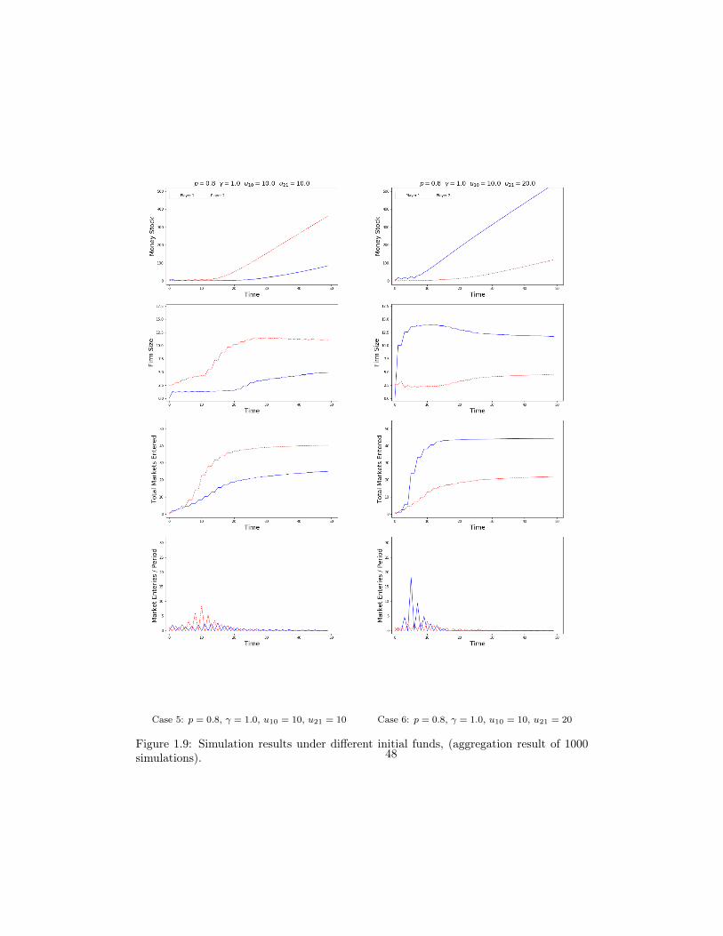
Case 5: p = 0.8, γ = 1.0, u10 = 10, u21 = 10 Case 6: p = 0.8, γ = 1.0, u10 = 10, u21 = 20
Figure 1.9: Simulation results under different initial funds, (aggregation result of 1000simulations). 48

Case 5: p = 0.8, γ = 1.0, u10 = 10, u21 = 10 Case 6: p = 0.8, γ = 1.0, u10 = 10, u21 = 20
Figure 1.10: Simulation results under different initial funds, (one special case).49

Case 7: p = 0.8, γ = 1.0, u10 = 20, u21 = 20 Case 8: p = 0.8, γ = 1.0, u10 = 20, u21 = 40
Figure 1.11: Simulation results under different initial funds, (aggregation result of 1000simulations) 50

Case 7: p = 0.8, γ = 1.0, u10 = 20, u21 = 20 Case 8: p = 0.8, γ = 1.0, u10 = 20, u21 = 40
Figure 1.12: Simulation results under different initial funds, (one special case).51

Chapter 2
Dynamic pricing solves the urban
transportation disparity -
Evidence from NYC on-demand
ride-sharing drivers
2.1 Introduction
Ride-sharing platforms have introduced a more efficient matching technology
than traditional taxis. The core of this matching scheme is the dynamic pricing system,
based on Uber’s official blog (Uber 2018): surge pricing is base fare multipliers generated
automatically from the platform’s back-end algorithms; it is a real-time location-based
pricing scheme, with the dual purpose of suffocating demand, boosting supply, and then
52

maximizing the number of completed rides. Because both the riders and drivers of ride-
sharing platforms are highly elastic (Uber 2014), we can observe the market equilibrium
change rapidly with respect to price changes.
Current and previous economic research on ride-sharing services focus more on
drivers’ behavior changes in working hours brought by the so-called "gig economy" (for
example, Chen and Sheldon (2016) and Hall, Horton, and Knoepfle (2017)), researchers
rarely investigate the real-time response of drivers to surge pricing, and how such pricing
scheme will affect the geographical disparity of pickups.
Hence, the purpose of this paper is two-fold: first, we aim to investigate how
drivers respond to price changes. To serve this purpose, we collect a significantly large
real-time dataset from the ride-sharing market-leading companies Uber and Lyft, for a
one-month period from New York City. We use the data to construct and estimate the
structural model of the drivers’ labor supply. Second, we aim to determine how the
dynamic pricing system makes a difference. To answer this question, we compute the
counterfactual case: what will happen to the city’s overall ride-sharing pickups if the
surge pricing is banned.
To more accurately capture the curvature of drivers’ supply, we use a non-
parametric instrumental variable estimation method (Horowitz 2011; Chetverikov, Kim,
and Wilhelm 2017; Chetverikov and Wilhelm 2017; Compiani 2018) to estimate the
transformed utility function, and we add a model constraint to the least square residual
minimization function to solve the ill-posed inverse problem that usually comes with the
non-parametric estimations. We find our final estimation results reasonable, significant,
and consistent.
We find that drivers’ labor supply are more elastic in non-Manhattan than Man-
hattan regions; and for both areas, drivers’ labor supply are more elastic when surge
53

pricing is equal to 1, implying that the emergence of price surges is a strong positive
incentive for drivers, (i.e., that a slight increase in price will cause drivers to work more).
We also find that the dynamic pricing system of ride-sharing platforms effec-
tively solves the geographical disparity problem of the taxi, and increases the overall
accessibility and pickups in the entire city. As calculated in our counterfactual case, if
there is no dynamic pricing, platform drivers will be crowded in the Manhattan area as
taxi drivers. Further, 27% of the total supply will be lost, including a significantly large
59% reduction in the non-Manhattan area, and, due to an in-flow of drivers from other
areas, Manhattan’s supply will only fall by 3%.
2.1.1 Literature and contribution
First, this paper contributes to the growing literature on supply-side analysis
of ride-sharing services. Camerer et al. (1997) find the estimated wage elasticity of
taxi drivers to be significantly negative and conclude that taxi drivers’ supply behavior
is consistent with target-earning. Farber (2015) replicate and extend the analysis in
Camerer et al. (1997) using data from taxi trip records in NYC for the five years from
2009 to 2013. His results negate previous the "weather shock – demand increase – hourly
wage increase – drivers fulfill income target – work less" explanation for less taxi supply
during rainy days in NYC; instead, he reports a positive estimated labor supply elasticity
and concludes that taxi drivers work less on rainy days possibly because it is unpleasant
to drive in the rain, and that "there is no additional benefit in continuing to drive". In
contrast, in this paper, from our estimation results, ride-sharing drivers in fact eager
to drive on rainy days, with the coefficient of "rain" in our structural utility function
being positive and significant. Chen and Sheldon (2016) conduct a similar approach
to study the working hour decision of Uber drivers using UberX partners’ data from
54

multiple cities, and they also report a positive labor supply elasticity: in response to
surge pricing, drivers choose to extend their sessions and provide more rides on the
Uber platform. Hall, Horton, and Knoepfle (2017) examine the long-run labor market
outcomes when facing a change in the "base fare", they find that increase in base fare
causes no detectable increase in drivers’ long-run hourly wage, because drivers’ utilization
rate will also decrease, and the total trip quantity will fall.
Castillo, Knoepfle, and Weyl (2017) use theoretical and empirical evidence to
demonstrate that dynamic surge pricing can help avoid the so-called "wild goose chase"
problem while maintaining system functioning when demand is high. Cramer and Krueger
(2016) compare the efficiency of ride-sharing services with traditional taxis, and find that
UberX drivers work more hours and drive more miles, partially due to Uber’s surge pric-
ing system matching supply with demand more closely.
In this paper, we have a similar conclusion regarding drivers’ positive labor sup-
ply, but use a different structure of data. Rather than working schedule flexibility, we
focus on the effect of dynamic pricing on spatial mobility. In contrast to the tradi-
tional labor economic hourly-wage and working-hour model applied in previous litera-
ture, our structural model is more of a choice model approach, as adopted by McFadden
et al. (1973) and Berry (1994). We do not consider the drivers’ working choice in the
perspective of "One day at a time"; instead, we segment the drivers’ pickup decision
processes into 10-minute time intervals and estimate drivers’ instantaneous responses to
price changes.
This paper also contributes to the research on geographical transportation dis-
parities.(for example, Tomer et al. (2011) and Kaufman et al. (2014)). These authors
are in agreement that great economic and employment opportunities exist in the im-
provement of mobility inequity. Lam and Liu (2019) apply a similar approach but study
55

the consumer choice model and find that ride-sharing mitigates geographical disparity
in transportation by providing accessible ride-hailing service to low-accessibility neigh-
borhoods. In this paper, we focus on the effect of dynamic pricing on the supply side
and find a similar result that without surge pricing, ride-sharing drivers will primarily
concentrated in the airports and the Manhattan area, as do taxi drivers.
This paper can also be added to the emerging empirical applications of The con-
strained non-parametric instrumental variable estimation (NPIV) method. For example,
Chetverikov and Wilhelm (2017) estimate the gasoline demand from U.S. data; Compiani
(2018) estimates the structural demand function of strawberries using California grocery
store data. Both papers use a fully non-parametric approach in their empirical practices;
however, in this paper we add a parametric logit frame work to the non-parametric util-
ity function prior to conducting the estimation. This approach is adopted because, in
contrast to one or zero substitutes for target products in their cases, in the ride-sharing
case, for one single choice (one zone) defined in our model, there are too many substi-
tutes (253 zones) and we will have an excessive number of endogenous variables in one
equation if we use a fully non-parametric estimation method, a structural logit function
can help solve this problem.
The rest of the paper is organized as follows: In section 2, we introduce the
structural model that describes the behavior of drivers; In section 3, we explain the
data and data sources; In section 4, we explain the framework for empirical estimation;
Then, in section 5, we will introduce the constrained NPIV model used for estimation.
We calculate the counterfactual to test the influence of the dynamic pricing system in
section 6. Finally a conclusion is provided in section 7.
56

2.2 Structural Model
2.2.1 Setup
Consider a decision process described by the following decision tree in Figure
2.1: A driver i at the beginning of his workday makes decisions on the following: 1)
whether to drive or not; 2) whether to drive for Uber or Lyft; 3) (at each time t) which
zone to offer service. And these decisions don’t need to occur at the same time.
Driver i
Not drive
Zone : 1, 2, 3.....
Uber
Zone : 1, 2, 3.....
Lyft
Drive
Figure 2.1: Decision tree of representative driver i
Drivers use time and effort to exchange for service payment. In 2016, Uber and
Lyft only allowed drivers to see the pickup locations of the riders; no information of the
destinations were available when they made the pickup decision. Therefore, drivers were
not aware of the actual price of each trip, and, they could only see the Surge Multiplier
of each pricing zone.
The indirect utility of a driver i at time t to do a pickup in location j from
57

platform s is specified as:
Uisjt = f(SurgeMultipliersjt, X1sjt) +X2
sjt′β − γDistanceijt + ξsjt + εisjt (2.1)
Where X = {X1sjt, X
2sjt} represents a vector of location-time-platform, specified
exogenous characteristics that affect utility. Distanceijt is the travel distance for driver
i to zone j from his current location at time t. ξsjt is the unobserved (to researchers)
location-time-platform-specified utility component common to all drivers, εisjt is an i.i.d.
driver’s idiosyncratic utility term. Although drivers do not directly observe the actual
service price, they do know the surge pricing, the structural form of how the Surge
Multiplier entering the utility function is unclear, and we thus assume that it enters the
utility function in a non-parametric manner: f(.). Due to revealed preference, drivers are
going to make one pickup choice that gives the highest utility each time. Assuming that
εisjt are distributed in Type I extreme-value distributions, the discrete choice model is a
nested logit. Let δsjt represent the average utility of doing the pickup through platform
s in location j at time t:
δsjt = f(psjt, X1sjt) +X2
sjt′β − γDistancejt + ξsjt (2.2)
Where psjt is short hand for SurgeMultipliersjt. Note, here ξsjt is the structural
error; according to Berry (1994), it is not the difference between the predicted value and
the actual value. Also, we expect ξsjt to be correlated with psjt, particularly in a high
trading frequency two-sided market setup, where the market equilibrium depends greatly
on both supply and demand sides. The number of pickups in location j from platform s
58

as a proportion of the potential market at time t is:
Ssjt =eδsjt
1 +∑s
∑j eδsjt
(2.3)
Where we assume that the utility of outside option is 0, so that eδ0 = 1.
2.3 Data
We collect a substantial amount of data from different sources, for a one-month
period from June 1st 2016 to June 30th 2016, for New York City. Because the main data
source New York City TLC (Taxi Limousine Commission) divides the city into 263 zones
(we have data for 253 out of 263 of these zones), and reports their data accordingly, in
this paper, I will follow the same spatial segmentation rules for all location-based data.
Also we aggregate and average the data into 10-minute time intervals. For June 2016,
the total number of time intervals will be 30 × 24 × 6 = 4320, and the full-balanced
panel dataset will have 4320 × 253 × 2 = 2194560 observations. Further, all data listed
below are collected and processed accordingly, and the summary statistics can be found
in Table 2.1. In our research we will focus on service type "UberX" and "Lyft" because
they are viewed as close substitutes to taxi.
Table 2.1: Summary Statistics
Variable Mean Std. Dev. Min 5% 25% 50% 75% 95% Max
Surge multiplier 1.077 0.204 1 1 1 1 1 1.525 5Rain 0.025 0.156 0 0 0 0 0 0 1Aver. trip distance 3.999 2.658 0.267 2.089 2.720 3.386 4.308 8.635 21Aver. tips 1.988 2.013 0.023 0.425 1.071 1.602 2.071 5.437 26Pickups 3.074 6.491 0 0 0 1 3 15 151EWT 279.156 158.192 78 120 180 240 330 540 3750
59

1. Real time Uber and Lyft data
First, we request a significant amount of real-time API data from Uber and Lyft for
every 2 to 3 minutes, including surge multiplier and expected waiting time (EWT)
for all service types available at the geographical central point of each zone. Uber
changes its price more smoothly, for a rate of 0.1 each time; in contrast, most likely
due to an unstable market condition caused by fewer users, Lyft changes its price
more aggressively and more frequently for a rate of 0.25 each time.
2. New York City TLC Uber and Lyft trip records
New York City TLC provides For-Hire-Vehicle ("FHV") trip records, which capture
pick-up date, time, and taxi zone Location ID. We identify "UberX" and "Lyft"
from the trip records by maintaining the base category "community car".
3. New York City TLC Taxi records
Although little information was given from the FHV trip records, New York City
TLC provides highly detailed data of taxi trip records. For each trip, it records:
pick-up and drop-off coordinates, number of passengers, trip distance, trip duration,
trip fare, tips received, method of payment, etc.
4. Central Park Weather
Wunderground.com reports detailed New York Central Park weather conditions
on an hourly basis, in order to capture the most important features; as well as
considering the computation difficulty, we only include the dummy for "rain" at
the current hour.
5. Subway Status
Subway status is acquired from the website Subwaystats.com, which updates the
status information of every NYC subway line every 5 minutes, and report the sub-
60

way status in 5 categories :"Good service", "Delay", "Planned Work", "Service
Change", and "Suspended". In my data, when a certain zone has several subway
line across it, we will only record the most severe case within this 10-minute time
interval. For example, if "Good service" and "Service Change" occur for two sub-
way lines in the same zone at the same time, we will record "Service Change", this
rule also applies if there is a status transition within the 10-minute time interval.
2.4 Empirical Framework
2.4.1 Setups
Definition of Markets
We define the market t, based on the level of 10-minute time interval, and the
choice set (products) is defined as zones and platforms to provide services, as in Figure
2.1.
Utility Transformation
We use the maximum total pickups of all zones in a 10-minute time interval as
our size of potential market, which is 3,107 in our data.
We use this number to calculate the market shares, then, use the inversion
method to calculate the average utility values:
δsjt = logSsjt − logS0 (2.4)
Where S0 is the market share of the outside option.
61

Ones and Zeros
One problem with the data is that, referring to Table 2.1, almost 75% of the
time, there is no surge pricing at all. Further, platforms do not allow for the surge
multiplier to be less than 1, hence there are excessive number of ones in the data. Thus,
we could face two problems: first, we cannot identify the true equilibrium price, when
surge multiplier equals 1, because there might be the case of supply access, the actual
equilibrium surge price might be less than 1, and we have no track of it. Second, when
we average the coefficients when surge price equals to 1, because of the price floor, the
actual supply conditional on price could be more than the recorded pickups; therefore,
we are under estimating the driver’s utility.
We attempt to solve this problem by identifying the case when surge pricing is
at the right tail of being 1: we maintain the data for the surge multiplier to be equal to
1 (psjt = 1) at time t, iff at time t + 1, at the same location, a surge multiplier larger
than 1 (psjt+1 > 1) occurs.
We also drop all Ssjt = 0 in our data set, because in the above utility transfor-
mation process, ln(0) does not exist.
Supply Shifters
We divide the daily 24 hours into 8 time blocks as Lam and Liu (2019), including:
Morning rush (weekdays 7a.m. - 9 a.m.), evening rush (weekdays 4 p.m. - 7 p.m.),
weekday day time (weekdays 10 a.m. - 3 p.m.), weekday night (weekdays 8 p.m. - 11
p.m.), weekday late night (0 a.m. - 6 a.m.), weekend day time (weekends 5 a.m. - 5
p.m.), weekend night (weekends 8 p.m. - 11 p.m.), and weekend late night (weekends
0 a.m. - 4 a.m.). We also separate the regression into Manhattan and non-Manhattan
areas.
62

Besides surge multiplier, we include the following variables as exogenous supply
shifters: 1) The average tips paid by taxi passengers within each time block of each zone;
2) whether it is raining in the current 10-minute time interval; 3) the average taxi trip
distance of passengers within each time block of each zone; 4) dummies for Uber and
airports.
By setting these supply shifters, we assume that 1) although the drivers could not
have specific knowledge on each trip, he/she at least has some expectation related with
time and location; 2) taxi and ride-sharing platforms are sharing a similar distribution
of customers, therefore, their behavior patterns are similar for us to use as proxies for
ride-sharing platforms.
Independence of Irrelevant Alternatives(IIA)
We choose to use the nested logit framework in this paper, and since Uber and
Lyft are providing almost identical services, we assume the nest dissimilarity factor to
be 1 for both Uber and Lyft, mathematically indicating that the products are equally
similar within and across platforms. This setup will reduce our estimation framework to
a simple multinomial logit. Instead, we add a dummy variable for Uber = 1 to capture
the difference between platforms. Moreover, because we do not have the data regarding
driver’s demographic information, we cannot take into account the random utilities in our
regression; However, this approach is sensible, because we are looking at the overall effect
of the dynamic pricing system, and thus, estimating the average effect could sufficiently
serve our research purposes.
63

2.4.2 Identification
Because of the high trading frequency in the two-sided platforms, the supply and
demand could be highly volatile, thus our estimation is subject to the price endogeneity
problem. We construct the instrumental variable for the surge multiplier using the aver-
age local expected waiting time and the local subway status within the 10-minute time
interval. Where the expected waiting time was also acquired from Uber and Lyft’s API,
it is a variable in the unit of seconds measuring the estimated waiting time for a pickup
prior to a rider sending out the request. This one can only be observed by the riders;
therefore, no drivers have any prior knowledge regarding where the request is sent from
or if the driver is being matched for this request. Another advantage of using expected
waiting time as the instrumental variable is that this one has a lot of variations (refer
to table 2.1). However, one problem with this instrumental variable is that, it is related
to overall demand access of all riders and drivers in the nearby zones, thus, although
an individual driver cannot observe it, it is still in some degree reflecting some general
information regarding changes in the preferences of surrounding drivers.
Another potential instrument is the subway status, which is supposed to be a
valid instrumental variable because subway status is proposed as being independent of
ride-sharing supplies. However, there are two problems with these variables as instru-
ments: first, not all zones have subway lines running across them, (refer to Figure 2.4)
only 185 out of 253 zones have at least one subway station inside. The second problem
is that they are lack of variation.
Due to the fact that there will be transformations of our variables into B-spline
bases in the estimation process, the instrumental variables are required to have at least
one continuous variable, and the current expected waiting time data from the API has
some endogeneity issue. We address this problem by fitting the expected waiting time
64

with subway status, and other location, time and platform characteristics. And use the
fitted expected waiting time (EWT ) as our final instrumental variable. The purpose of
this approach is to capture the parts in the expected waiting time that are due to the
changes in subway status; for example, a delayed train in the nearby subway station,
could lead to a positive demand shock at the current location, hence increasing the local
expect waiting time for ride-sharing requests.
Table 2.2: First-stage Linear Regression
Manhattan Non-ManhattanSurge Multiplier Coefficient Coefficient
EWT -0.000215∗∗∗ -0.000190∗∗∗(-51.50) (-115.36)
Rain 0.0163∗∗∗ 0.0349∗∗∗(6.42) (24.17)
Average local trip distance -0.00897∗∗∗ 0.00035∗∗∗(-20.92) (4.92)
Average local tips 0.00223∗∗∗ -0.000403∗∗∗(4.48) (-6.45)
Uber -0.114∗∗∗ 0.0111∗∗∗(-176.14) (-36.29
Airport - -0.000579- (-0.26)
Constant 1.239∗∗∗ 1.126∗∗∗(892.42) (1980.43)
R2 0.0672 0.0109F − statistic 8770.77 3246.47
*** denotes p -value< 1% significance level based on robust standard error
The BLP type instruments (Berry 1994; Berry, Levinsohn, and Pakes 1995),
such as sum of surge prices of UberX and Lyft in the surrounding zones, or sum of surge
prices of other types of services in the surrounding zones, is not applicable here, probably
due to several reasons: 1) surge prices are generated from the same platform algorithm,
there could be a problem of tautology; 2) there is a lack of variation in the BLP type
instruments, because the values of surges are equal to 1 for most of the time; and 3)
there is a spatial correlation among zones, one regional shock may alter the supplies and
65

prices of several adjacent zones together, such as traffic jams, and hence the surge prices
of surrounding zones are also correlated to the local supply. Because of the problems
listed above, we cannot use these variables as instruments.
We report the linear first-stage regression coefficients in Table 2.2.
2.4.3 Spatial Disparity
Another problem with estimating the structural model is that: drivers’ pickup
decision at time t are in fact depends on their previous drop-off location, which means
that the distribution of drivers at the beginning of time t, affects the market share of
each zone at time t, but we do not have the trip-level drop-off coordinates in our data,
and hence cannot estimate the γDistancejt term in our structural model. To solve
this problem, we assume that the average distance for drivers to all jt is a constant
(Distancejt is a constant). This assumption requires drivers to be equally distributed
for all markets ∀t ∈ T . Hence, we do not consider the spatial disparity in our estimation,
and the distance term enters the structural model as a constant α:
δsjt = f(psjt, X1sjt) +X2
sjt′β − α+ ξjt (2.5)
Where α = γDistancejt.
We also assume that at each time t, drivers are making decisions among all zones
in the New York City area, an assumption which may actually not be the case, referring
to Uber and Lyft, their algorithms automatically match up drivers with nearby riders,
and typically the decisions drivers can make is whether to accept a job or not. But
according to surveys by Lee et al. (2015): "...drivers strategically controlled when and
where to work and when to turn on the driver mode of an app to get the types of requests
66

and clienteles that they preferred: limiting the area that they worked in by turning off
the driver mode...", the authors also find that drivers do not chase surge if the surging
area is too far away, because the surge pricing changes too rapidly, and may therefore
disappear by the time they arrive.
Thus, we consider that the spatial disparity problem for one time t, should not
make our final estimation results invalid, because we are examining the average results
over many time periods (4320); although the distributions of drivers is not even at one
time t, the overall aggregate distribution should be, for 4320 time periods (markets).
If we look at the taxi drop-off map in June 2016, Figure 2.6, the drop-off locations
are more evenly distributed than the pickup locations, also, there is a clear difference
between Manhattan and non-Manhattan areas, and we already capture the difference in
our estimation. Hence, our final estimation result for an average influence of distance
should be valid.
2.5 Estimation
2.5.1 Constrained NPIV estimator
Objective Function and Constraint
We use the constrained NPIV(non-parametric instrumental variable) method
introduced by Chetverikov and Wilhelm (2017), to estimate our structural model. In this
structural model we assume that all the exogenous parts enter the model in a separable
linear way such that:
67

δjt = f(pjt) +X ′β − α+ ξsjt, E(ξsjt|Z,X) = 0 (2.6)
ξsjt = δjt − f(pjt)−X ′β + α (2.7)
Where Z is a vector of instrumental variables. In this paper, Z is the parts of
a consumer’s expected waiting time explained by current subway operation status. We
want to estimate the function f(.) based on random samples generated from {δ, P,X,Z}.
Consider a series estimator, let {gk(p), k ≥ 1} , {qk(z), k ≥ 1} be two orthonormal
bases in L2[0, 1] space, let g(p) := (g1(p), ..., gK(p))′ and q(z) := (q1(z), ..., qJ(z))′ for
J ≥ K ≥ 1, be two vectors of basis functions. DefineG := [g(p), X],Q := [q(z), q(z)×X].
Where q(z)×X is the tensor product of q(z) and X , that, it is the intersections of q(z)
with exogenous variables X.
Consider the general "law of supply"; we are expecting the driver’s utility to
be positively correlated with the price, and therefore the first order of f(p) should be
positive such that: df(p)dp > 0. The constrained estimator from moment condition is:
minθ
(δ −Gθ)′Q(Q′Q)−1Q′(δ −Gθ) (2.8)
subject todf(p)
dp> 0 (2.9)
Where θ = [θp, β, α], θp (K×1) is the coefficient vector of non-parametric basis functions
of p. Note here, that we construct an estimator of f(p) as a linear combination of basis
functions that: ˆf(p) = g(p)′θp. Because X is a vector of exogenous variables, dXdp = 0,
the constraint can also be written as dg(p)dp θp > 0.
68

Regression Parameters
To estimate the utility function, we use a power 2 B-spline basis for both en-
dogenous and instrumental variables, as in Chetverikov and Wilhelm (2017), and the
number of knots on both splines are chosen by cross validation based on the criteria of
minimizing MSE; the computation complexity is also taken into consideration that the
maximum knots test by cross validation is 7. Finally we choose the number of knots to
be 6 for both instrumental and endogenous variables.
Robustness Check
In order to exclude the outliers in our data, in our regression, we keep 1− 99%
percentile of the surge multipliers, such that the surge multipliers in our estimation data
falls into the range of [1, 3].
Moreover, to test the robustness of the non-parametric estimation, we evenly
divide the surge multiplier into 0.1-length intervals, and within each surge pricing interval,
we randomly draw 1,000 observations; then we repeatedly (100 times) estimate the model
on these random subsets.
We compare among the estimation methods - constrained NPIV, unconstrained
NPIV and linear regression, using regression results from the 100 subsets (refer to Ap-
pendix C for comparison), and find that the performance of the constrained NPIV is the
best among the three, with the lowest coefficients standard errors (consistent), and the
highest probability of significance.
Estimation Method
We use a two-step estimation method to capture the non-parametric and para-
metric parts in the structural model separately:
69

In the first step, we estimate the entire model as in Equation 2.9, to get θ =
[θp, β, α]; In the second step, we extract the non-parametric part from δsjt, and use OLS
to regress the residuals on the other supply shifters:
ˆResidual = δsjt − g(p)′θp (2.10)
For unknown reason, in practice, we find that if we reverse the order in step 2,
as Chetverikov and Wilhelm (2017) do in their working paper: extract the linear part
X ′β − α first, then re-estimate the non-parametric part f(p) using NPIV, we tend to
under estimate the utility.
2.5.2 Estimation Results
The estimated non-parametric B-spline coefficients are reported in Table 2.3.
Table 2.3: Estimation Results of Non-parametric B-spline Knots
N=100 Knot 1 Knot 2 Knot 3 Knot 4 Knot 5 Knot 6
Manhattan
Average -6.91935 -6.61819 -6.61637 -6.61637 -5.82712 7.438699Std. Err. 0.693959 0.145532 0.14491 0.14491 0.922791 4.525964
95% Conf. Interval -6.8496 -6.60356 -6.6018 -6.6018 -5.73437 7.893575-6.98909 -6.63281 -6.63093 -6.63093 -5.91986 6.983822
Non-Manhattan
Average -9.36882 -6.79264 -6.38106 -5.34883 -5.30653 -5.24012Std. Err. 2.152473 0.713096 0.602384 0.489985 0.516812 0.815026
95% Conf. Interval -9.15248 -6.72097 -6.32052 -5.29959 -5.25459 -5.15821-9.58515 -6.86431 -6.4416 -5.39808 -5.35848 -5.32203
Due to the fact that the coefficients of non-parametric part f(p) is complicated
and also difficult to explain, we also report the curves of fitted f(p) for Manhattan and
70

non-Manhattan areas in Figure 2.2. Recall that we assume drivers to have the same price
sensitivity for both platforms.
We can see that holding other things constant, when surge pricing is low, the
Manhattan area is more attractive for drivers, but the drivers are less sensitive to price
here than they are in the non-Manhattan area.
The coefficients of the linear supply shifters are concluded in Table 2.4, we report
the one with the highest R2 from 100 estimations. As expected, the constant term α for
the average effect of pickup distance is negative, that drivers do not like to do pickups
far from their current location, it is also reasonable that αManhattan > αnon−Manhattan,
because it is clear that geographical zones in Manhattan area are closer to each other than
zones in other areas, and there are in general more pickups in Manhattan than in other
areas that: DistancejtManhattan
< Distancejtnon−Manhattan
, so holding parameter −γ
constant for Manhattan and non-Manhattan areas, it is reasonable to see that the average
effect of distance in the non-Manhattan areas to be relatively larger.
In general, drivers do not like the zones with higher average trip distance, and
prefer the zones with higher average tips; also, drivers favor Uber more than Lyft. Sur-
prisingly, different from what Camerer et al. (1997) and Farber (2015) find in their papers
for taxi drivers, "Rain" is in fact an incentive for platform drivers — they are more willing
to offer rides on rainy days.
All coefficients are significant at the 1% significance level.
2.5.3 Elasticity of Supply
We calculate the average supply elasticity use equation:
Elasticity =df(p)
dpp(1− Ss) (2.11)
71

Table 2.4: OLS Estimation Results of Linear Part
Manhattan Non-Manhattan
Variable Coefficient Coefficient
Rain 0.642∗∗∗ 0.390∗∗∗(6.33) (6.18)
Mean local trip distance -0.467∗∗∗ -0.0782∗∗∗(-17.30) (-10.56)
Mean local tips 0.722∗∗∗ 0.0474∗∗∗(12.51) (4.91)
Uber 1.822∗∗∗ 0.965∗∗∗(48.22) (41.46)
Airport - 2.191∗∗∗- (17.01)
Constant -0.218∗∗∗ -0.312∗∗∗(-2.81) (-11.04)
R2 0.3039 0.1928F − statistic 710.65 484.25*** denotes p -value< 1% significance level based on robust standard error
Where Ss is the average share of platform s for all zones and all markets. How-
ever, because both Uber and Lyft’s average market share are particularly small compared
to 1, which makes little difference when doing (1 − Ss), the actual elasticity difference
between the two platforms are extremely trivial, so we consider drivers’ average supply
elasticity to be the same for both platforms.
72

Figure 2.2: Fitted Nonlinear part: f(p)
Figure 2.3: Estimated Supply Elasticity
The estimated supply elasticity is reported in Figure 2.3. We can see that for
both Manhattan and non-Manhattan areas, the supply is more elastic at the point where
surge equals 1, which imply that the emerging of price surging is a strong incentive for
drivers to offer more rides, especially for drivers in the non-Manhattan area. We can also
observe that on average drivers’ supply in the non-Manhattan area is more elastic than
73

it is in the Manhattan area.
One problem with the estimated elasticity is that there are many "kink" points;
this issue is due to unsmooth derivatives of B-spline specified g(p)′, clearly, each "kink"
point corresponds to one B-spline "knot" in Figure 2.3, this problem can be regarded as
an ill-posed inverse problem caused by specific functional form. But the general trend
and range of drivers’ labor supply elasticity should be in good shape.
Another issue is the fitted f(p) and supply elasticity for Manhattan area signifi-
cantly increasing after SurgeMultiplier > 2.5. It is potentially due to two reasons: first,
we have few (only 1.5K) observations after this point, and hence the sampling process
cannot mitigate the errors in different estimations, a small fluctuation in the spline will
cause the estimated elasticity to deviate from the truth. Second, this issue may also
due to that the variation in our instruments fails to control for the endogeneity when
SurgeMultiplier > 2.5.
2.6 Counterfactual
In this section, we use the previous estimation results to test the influence of
Uber and Lyft’s dynamic pricing system, and ask: what if surge pricing is banned?
The counterfactual results are summarized in Table 2.5, we can observe that if
there is no surge pricing, in June 2016 NYC, the total supply of ride-sharing platforms
will decrease by more than 27%. Uber would lose almost 27% of the supply, compared
with 25% for Lyft.
Also, supply in the non-Manhattan areas would be damaged more by losing more
than 59% , and the Manhattan area will only lose approximately 4%, because without
surge pricing, most of the drivers would prefer to work in the Manhattan area, drivers
74

Table 2.5: Counterfactual: What if surge pricing is banned?
Real Pickups Counterfactual ∆ ∆%
Uber 5346025 3863178 -1482847 -27.74%Lyft 1073680 799757 -273923 -25.51%
Manhattan 3699627 3558715 -140912 -3.81%Non-Manhattan 2720078 1104220 -1615858 -59.41%
Total 6419705 4662935 1756770 -27.37%
from the non-Manhattan area will flood into Manhattan, and offset previous losses. The
result of forbidding surge pricing will be more clear if we compare the two figures in Figure
2.7: Most of the previous non-Manhattan rides would flood into Manhattan borough,
and the dark purple zone with most pickups in the corner of Manhattan borough is the
Randalls Island, it is the famous recreation center in Manhattan area, as seen in Figure
2.4 and Figure 2.5, there is no subway line across this island, with people visiting there
on average being willing to pay more tips. Thus, in our counterfactual case, Randalls
Island will be the most attractive place for drivers.
Moreover, if we compare the counterfactual map with the aggregate taxi pick-ups
in Figure 2.6, they are highly similar, with most of the pickups concentrating in lower
Manhattan, and the lights being relatively dim in other boroughs, except for the airports.
This result implies that the dynamic pricing system is the key reason explaining why ride-
sharing drivers distribute more evenly in the urban area than taxi drivers, increasing
overall accessibility of the entire city and effectively re-distributing the drivers.
2.7 Conclusion
In this paper, we investigate the effect of the dynamic pricing system on ride-
sharing platform drivers’ labor supply decisions. Rather than working-hour and wage-
75

rate relations explored by previous literature, we examine the instantaneous response of
drivers to price surges. Using data from New York City, we estimate the structural choice
model through a constrained non-parametric instrumental variable (NPIV) approach. We
use the estimated coefficients to calculate the drivers’ supply elasticity and compute the
counterfactual case involving the following question: What will happen to drivers if the
surge pricing system is banned?
We find that:
1. Drivers prefer Uber to Lyft;
2. Drivers like to do pickups in areas that pay more tips;
3. The emergence of a price surge is a highly strong incentive for drivers, such that
the supply is more elastic at the point SurgeMultiplier = 1;
4. Different from what Camerer et al. (1997) and Farber (2015) find in their papers,
drivers are more willing to serve during rainy days;
5. The dynamic pricing system effectively solves the geographical disparity problem
faced by the taxi industry, helping to re-distribute the drivers and increasing the
overall accessibility of the entire New York City area: without dynamic pricing,
platform drivers would be crowded in the Manhattan area;
6. Without dynamic pricing, the total supply in June 2016 NYC would decrease by
27%, among which, more than 59% of the non-Manhattan supply would be lost;
7. Due to an in-flow of drivers from other areas, supply in Manhattan will only reduce
by 3%.
Finally, I would like to mention one limitation of this paper: we did not consider
the long-term endogenous behavioral changes of drivers, and it is possible that the actual
76

impact of forbidding dynamic pricing would be more severe; when drivers know that there
is no dynamic pricing, their expected hourly income would decrease, and they would
choose to leave the market, and hence the overall potential market size would shrink.
And for those who stay in the industry, they will have to increase their utilization rate
to meet their previous wage level, causing a further decrease in drivers’ welfare.
77

2.8 Tables and Figures
Figure 2.4: Average Local Surge Multiplier & Subway Maps.
78

Figure 2.5: Average Local Tips & Average Local Trip Distance.
79

Figure 2.6: Aggregate taxi pickups and drop-offs in June 2016, NYC.
80

Figure 2.7: Real ride-sharing pickups and the counterfactual pickups in June 2016, NYC.
81

Appendices
82

Appendix A Notations for Chapter 1
Table 6: Notations
Notation Definitioni, j index for markets
n, -n index for players
N, M Base amount of demands and supplies in one city
t index for time/period
K Cities’ rank on population
αK Average return per transaction in the Kth market
γ Degree of network effect
−h Switching cost
V Average utility per transaction
p Degree of second mover disadvantage
r Depreciation rate
c Cost constant
F Set for all feasible markets
Xnt Set for occupied markets for player n at time t
It Set for markets with 1 player at time t
Jt Set for markets with 0 player at time t
yit Decision variables for market i ∀ i ∈ It at time t
zjt Decision variables for market j ∀ j ∈ Jt at time t
z∗t , y∗tz∗t , y∗tz∗t , y∗t Player n’s optimal choice set at time t
unt Player n’s money stock at time t
mnt Player n’s total market size at time t
xnt Player n’s size ratio at time t
Snt Player n’s market share at time t
Rnt Player n’s total revenue from all occupied markets at time t
Cnt Player n’s total entry cost at time t
83

Appendix B Proofs for Chapter 1
Proof of Proposition 1
NM(K+1)2E(α) +S11
NMK2 αk >
NM(K+2)2E(α) +S11
NMK2 αk, so, Player 1 will choose K+1 when
Player 2 chooses K. And NM(K+1)2E(α) + NM
K2 αk > S10NM
(K+2)2E(α) + NMK2 αk so Player 1
will choose K+1 when Player 2 chooses K+2.
When Player 2 chooses K+1, Player 1 also chooses K+1, iff S10NM
(K+1)2E(α) + NMK2 αk >
NM(k+2)2E(α) + NM
K2 αk, so S101
(K+1)2 > 1(K+2)2 , (K+2
K+1 )2 > 1S10
, since S10 ∈ [0.5, 1],
K < 2√S10−1
1−√S10
, 2√S10−1
1−√S10
is monotonically increasing in S10 ∈ [0.5, 1], the threshold K
for Player 1 chooses K+1 is increasing with S10
Proof of Proposition 2
When Player 1 chooses K+1, the size of (1−s1)NMK2 αk, (1−s1) NM(K+1)2E(α) and NM
(K+2)2E(α)
is changing with K, γ and αK , E(αK), So all three actions are possible best responses.
When Player 1 chooses K+2, same as above.
Proof of Proposition 3
From Proposition 1 and 2, when K+1 is the dominant strategy for Player 1, there are
three PSNEs. When Player1 has the incentive to deviate to K+2, there will be 2 anti-
coordinates PSNEs and 2 MSNEs.
84

Appendix C Estimation methods comparison for Chap-
ter 2
Table 7: Summary statistics of coefficients under different estimation methods
(based on estimation results from regressions on 100 sub-samples)
Surge Rain Distance Tips Uber Airport Constant
Constrained non-Manhattan
Mean - 0.597 -0.077 0.050 0.936 2.030 -0.525SD - 0.062 0.006 0.008 0.024 0.144 0.148Min - 0.432 -0.094 0.029 0.876 1.751 -0.927Max - 0.803 -0.062 0.067 0.999 2.440 -0.165
NPIV Manhattan
Mean - 0.493 -0.459 0.722 1.821 - -0.110SD - 0.076 0.025 0.042 0.030 - 0.068Min - 0.351 -0.529 0.637 1.759 - -0.330Max - 0.674 -0.408 0.810 1.930 - 0.000
NPIV
non-Manhattan
Mean - 0.639 -0.090 0.036 0.921 1.985 -0.906SD - 0.131 0.016 0.020 0.059 0.280 0.297Min - 0.276 -0.127 -0.022 0.812 1.277 -1.665Max - 0.965 -0.041 0.085 1.088 2.944 -0.286
Manhattan
Mean - 0.496 -0.463 0.719 1.824 - -0.145SD - 0.110 0.038 0.064 0.041 - 0.148Min - 0.208 -0.535 0.505 1.740 - -0.524Max - 0.722 -0.340 0.904 1.970 - 0.186
Linear non-Manhattan
Mean 19.628 -6.370 -0.172 -0.262 -0.817 4.694 -38.681SD 118.042 41.206 0.571 1.351 10.415 16.421 194.478Min -510.278 -310.226 -4.798 -8.387 -79.575 -60.217 -1421.660Max 861.414 175.624 1.924 5.872 40.062 130.538 839.827
Regression Manhattan
Mean -2.460 1.041 -0.762 1.197 1.898 - -1.927SD 1.059 0.260 0.139 0.209 0.049 - 1.961Min -6.686 0.659 -1.261 0.839 1.772 - -4.965Max -0.785 2.140 -0.529 1.881 2.041 - 5.956
85

Table 8: Percentage of significant coefficients under different estimation methods
(based on estimation results from regressions on 100 sub-samples)
Surge Rain Distance Tips Uber Airport Constant
Constrained non-Manhattan10% level - 100% 100% 100% 100% 100% 100%5% level - 100% 100% 100% 100% 100% 100%1% level - 100% 100% 100% 100% 100% 100%
NPIV Manhattan10% level - 100% 100% 100% 100% - 42.42%5% level - 100% 100% 100% 100% - 31.31%1% level - 100% 100% 100% 100% - 14.14%
NPIV
non-Manhattan10% level - 100% 100% 55.10% 100% 100% 100%5% level - 100% 100% 48.98% 100% 100% 100%1% level - 98.98% 98.98% 22.45% 100% 100% 100%
Manhattan10% level - 98.95% 100% 100% 100% - 46.32%5% level - 97.89% 100% 100% 100% - 37.89%1% level - 94.74% 100% 100% 100% - 28.42%
Linear non-Manhattan10% level 18.56% 7.22% 53.61% 0.00% 3.09% 50.52% 34.02%5% level 7.22% 3.09% 46.39% 0.00% 3.09% 44.33% 24.74%1% level 2.06% 0.00% 30.93% 0.00% 0.00% 32.99% 7.22%
Regression Manhattan10% level 62.11% 94.74% 96.84% 96.84% 100% - 30.53%5% level 38.95% 89.47% 96.84% 95.79% 100% - 18.95%1% level 7.37% 75.79% 89.47% 90.53% 100% - 14.74%
86

Constrained NPIV
NPIV
Linear Regression
Figure 8: Fitted f(p) under different estimation methods87

Constrained NPIV
NPIV
Linear Regression
Figure 9: Estimated supply elasticity under different estimation methods88

Bibliography
Anderson, Eugene W. 1998. “Customer satisfaction and word of mouth.” Journal ofservice research 1 (1): 5–17.
Armstrong, Mark. 2006. “Competition in two-sided markets.” The RAND Journal ofEconomics 37 (3): 668–691.
Berry, Steven T. 1994. “Estimating discrete-choice models of product differentiation.”The RAND Journal of Economics: 242–262.
Berry, Steven, James Levinsohn, and Ariel Pakes. 1995. “Automobile prices in marketequilibrium.” Econometrica: Journal of the Econometric Society: 841–890.
Camerer, Colin, Linda Babcock, George Loewenstein, and Richard Thaler. 1997. “Laborsupply of New York City cabdrivers: One day at a time.” The Quarterly Journal ofEconomics 112 (2): 407–441.
Castillo, Juan Camilo, Dan Knoepfle, and Glen Weyl. 2017. “Surge pricing solves thewild goose chase.” In Proceedings of the 2017 ACM Conference on Economics andComputation, 241–242. ACM.
Chen, Le, Alan Mislove, and Christo Wilson. 2015. “Peeking beneath the hood of uber.”In Proceedings of the 2015 Internet Measurement Conference, 495–508. ACM.
Chen, M Keith, and Michael Sheldon. 2016. “Dynamic Pricing in a Labor Market: SurgePricing and Flexible Work on the Uber Platform.” In Ec, 455.
Chetverikov, Denis, Dongwoo Kim, and Daniel Wilhelm. 2017. “Nonparametic instru-mental variable estimation.”
Chetverikov, Denis, and Daniel Wilhelm. 2017. “Nonparametric instrumental variableestimation under monotonicity.” Econometrica 85 (4): 1303–1320.
Compiani, Giovanni. 2018. “Nonparametric Demand Estimation in Differentiated Prod-ucts Markets.” Available at SSRN 3134152.
89

Cramer, Judd, and Alan B Krueger. 2016. “Disruptive change in the taxi business: Thecase of Uber.” American Economic Review 106 (5): 177–82.
Dewenter, Ralf, Jürgen Rösch, et al. 2012. “Market entry into emerging two-sided mar-kets.” Economics Bulletin 32 (3): 2343–2352.
Farber, Henry S. 2015. “Why you can’t find a taxi in the rain and other labor supplylessons from cab drivers.” The Quarterly Journal of Economics 130 (4): 1975–2026.
Golder, Peter N, and Gerard J Tellis. 1993. “Pioneer advantage: Marketing logic or mar-keting legend?” Journal of marketing Research: 158–170.
Greenwood, Brad N, and Sunil Wattal. 2015. “An Empirical Investigation of Ride Sharingand Alcohol Related Motor Vehicle Homicide.” In Academy of Management Proceed-ings, 2015:17281. 1. Academy of Management Briarcliff Manor, NY 10510.
Hall, Jonathan V, John J Horton, and Daniel T Knoepfle. 2017. “Labor market equilibra-tion: Evidence from uber.” URL http://john-joseph-horton. com/papers/uber_price.pdf, working paper.
Hall, Jonathan V, and Alan B Krueger. 2018. “An analysis of the labor market for Uber’sdriver-partners in the United States.” ILR Review 71 (3): 705–732.
Hart, William E., Carl D. Laird, Jean-Paul Watson, David L. Woodruff, Gabriel A.Hackebeil, Bethany L. Nicholson, and John D. Siirola. 2017. Pyomo–optimizationmodeling in python. Second. Vol. 67. Springer Science & Business Media.
Hart, William E, Jean-Paul Watson, and David L Woodruff. 2011. “Pyomo: modelingand solving mathematical programs in Python.” Mathematical Programming Com-putation 3 (3): 219–260.
Horowitz, Joel L. 2011. “Applied nonparametric instrumental variables estimation.” Econo-metrica 79 (2): 347–394.
Insights, CB. 2014. “The top 20 reasons startups fail.” October 7:2014.
Jullien, Bruno. 2011. “Competition in multi-sided markets: Divide and conquer.” Amer-ican Economic Journal: Microeconomics 3 (4): 186–220.
Katz, Michael L, and Carl Shapiro. 1994. “Systems competition and network effects.”Journal of economic perspectives 8 (2): 93–115.
Kaufman, Sarah, Mitchell L Moss, Justin Tyndall, and Jorge Hernandez. 2014. “Mobility,economic opportunity and New York City neighborhoods.” NYU Wagner ResearchPaper, no. 2598566.
90

Kim, Byung–Cheol, Jeongsik Lee, and Hyunwoo Park. 2013. “Platform entry strategyin two-sided markets: Evidence from the online daily deals industry.” In Can be re-trieved at: http://www. econ. gatech. edu/files/seminars/Kim_Daily_Deals_Main,202013–08.
Klemperer, Paul. 1987. “The competitiveness of markets with switching costs.” TheRAND Journal of Economics: 138–150.
Lam, Chungsang, and Meng Liu. 2019. “Toward Inclusive Mobility: Ridesharing MitigatesGeographical Disparity in Transportation.” https://papers.ssrn.com/sol3/papers.cfm?abstract_id=2997190.
Lam, Wing Man Wynne. 2017. “Switching Costs in Two-Sided Markets.” The Journal ofIndustrial Economics 65 (1): 136–182.
Lambkin, Mary. 1988. “Order of entry and performance in new markets.” Strategic Man-agement Journal 9 (S1): 127–140.
Lee, Gwendolyn K. 2008. “Relevance of organizational capabilities and its dynamics: whatto learn from entrants’ product portfolios about the determinants of entry timing.”Strategic Management Journal 29 (12): 1257–1280.
Lee, Min Kyung, Daniel Kusbit, Evan Metsky, and Laura Dabbish. 2015. “Workingwith machines: The impact of algorithmic and data-driven management on humanworkers.” In Proceedings of the 33rd Annual ACM Conference on Human Factors inComputing Systems, 1603–1612. ACM.
Li, Ziru, Yili Hong, and Zhongju Zhang. 2016. “An empirical analysis of on-demand ridesharing and traffic congestion.”
Lieberman, Marvin B. 2005. “Did first-mover advantage survive the dot-com crash.”Unpublished working paper, UCLA.
Lieberman, Marvin B, and David B Montgomery. 1988. “First-mover advantages.” Strate-gic management journal 9 (S1): 41–58.
. 1998. “First-mover (dis) advantages: retrospective and link with the resource-based view.” Strategic management journal 19 (12): 1111–1125.
Lilien, Gary L, and Eunsang Yoon. 1990. “The timing of competitive market entry: Anexploratory study of new industrial products.” Management science 36 (5): 568–585.
McFadden, Daniel, et al. 1973. “Conditional logit analysis of qualitative choice behavior.”
Mitchell, Will. 1989. “Whether and when? Probability and timing of incumbents’ entryinto emerging industrial subfields.” Administrative Science Quarterly: 208–230.
91

Mitchell, Will. 1991. “Dual clocks: Entry order influences on incumbent and newcomermarket share and survival when specialized assets retain their value.” Strategic Man-agement Journal 12 (2): 85–100.
Peltier, Dan. 2016. “Uber and Lyft’s Growth Is Slowing in Most Major U.S. Cities@ONLINE.”https://skift.com/2016/10/12/uber-and-lyfts-growth-is-slowing-in-most-major-u-s-cities/.
Rochet, Jean-Charles, and Jean Tirole. 2003. “Platform competition in two-sided mar-kets.” Journal of the european economic association 1 (4): 990–1029.
. 2006. “Two-sided markets: a progress report.” The RAND journal of economics37 (3): 645–667.
Rysman, Marc. 2009. “The economics of two-sided markets.” Journal of economic per-spectives 23 (3): 125–43.
Seamans, Robert, and Feng Zhu. 2013. “Responses to entry in multi-sided markets: Theimpact of Craigslist on local newspapers.” Management Science 60 (2): 476–493.
Tomer, Adie, Elizabeth Kneebone, Robert Puentes, and Alan Berube. 2011. “Missedopportunity: Transit and jobs in metropolitan america.”
Uber. 2014. “A Deeper Look at Uber’s Dynamic Pricing Model.” http://abovethecrowd.com/2014/03/11/a-deeper-look-at-ubers-dynamic-pricing-model/.
. 2018. “How surge pricing works.” https://www.uber.com/en-ZA/drive/partner-app/how-surge-works/.
Wu, Brian. 2013. “Opportunity costs, industry dynamics, and corporate diversification:Evidence from the cardiovascular medical device industry, 1976–2004.” StrategicManagement Journal 34 (11): 1265–1287.
Xavier, Gabaix. 1999. “Zipf’s Law for Cities: An Explanation.” The Quarterly Journalof Economics 114 (3): 739–767. issn: 00335533, 15314650. http://www.jstor.org/stable/2586883.
Zhu, Feng, and Marco Iansiti. 2012. “Entry into platform-based markets.” Strategic Man-agement Journal 33 (1): 88–106.
Zipf, George Kingsley, et al. 1949. “Human behavior and the principle of least effort.”
92