Embed Size (px)
Citation preview
ESSENTIAL LibreOffice: Tutorials for Teachers
Copyright © Bernard John Poole, 2016. All rights reserved
150
5 MORE ON THE USE OF THE SPREADSHEET Making changes to existing spreadsheets
LEARNING OUTCOMES In Lesson 4 you created a grade sheet for a class of 4th graders based on a template you had put
together at the beginning of the same lesson. You learned that you can easily adapt a template for
use with other classes that you might teach. You learned also about the organization of
spreadsheets, about rows and columns, and the cells at the intersection of those rows and columns.
You learned how to select cells and how to address cells using row and column coordinates. You
learned how to enter formulas into certain cells in order to have Calc do calculations for you—
totals and percentages in particular.
You filled the rows and columns with labels and grades. You had a first introduction to the
idea that a spreadsheet can be a powerful tool for handling numeric data that requires mathematical
or statistical processing.
In this tutorial you will have the opportunity to reinforce what you learned in Lesson 4. At the
same time you will learn how to maintain a spreadsheet. This you will do by making enhancements
to the spreadsheet you created in Lesson 4.
You will also learn about some of the logical processing capabilities of spreadsheets,
capabilities which enable you to give an "intelligent" flavor to the applications that you build. In
particular, you will learn about the following features of Calc.
Updating an existing spreadsheet
Making changes to the look of a spreadsheet
Using the LOOKUP function
Creating charts based on spreadsheet data
Printing the updated spreadsheet
A caveat before you begin: You'll find it easiest to use the tutorial if you follow the directions
carefully. On computers there are always other ways of doing things, but if you wander off on your
own be sure you know your way back!
5.1 GETTING STARTED You're going to work with a Gradebook document very similar to the one you created in Lesson
4. If you completed Lesson 4, for the exercises that follow DO NOT USE the Gradebook Template
or Grade 4 2016 spreadsheet that you created in that lesson. For the sake of uniformity, and to
avoid confusion, you're going to use a Grade Book template and Grade Book spreadsheet specially
prepared for use with this lesson.
Lesson 5: More on the Use of the Spreadsheet
151
As an exercise at the end of the tutorial you will have the opportunity to incorporate these changes
into your own Gradebook documents (Grade4 2014 and Gradebook Template) which you created
when you completed Lesson 4.
You are going to make some improvements to the layout of the Gradebook, after which you
will learn about the LOOKUP function as an introduction to the logic capability of Calc. At the
end of the lesson you will learn how to create and modify charts of various kinds.
Open LibreOffice > Calc then make sure the storage medium (flash drive or external disk drive or hard drive) on which you have your Work Files for LibreOffice 5 folder is accessible
You are going to update two documents:
• a grade book template (called Gradebook Template, which is stored on your USB drive in
the Work Files for LibreOffice 5 folder > Miscellaneous Files folder > Templates folder);
• an actual grade book filled with data (this document has the name Gradebook and is stored
in the Work Files for LibreOffice 5 folder > Miscellaneous Files folder > Other Documents
folder)
You will work on the Gradebook document first.
By now you should know the steps to open a document, so go to your Work Files for LibreOffice 5 > Miscellaneous Files > Other Documents folder and Open the Gradebook document
Before proceeding with the tutorial, you need to save this spreadsheet on your USB drive in the
Data Files > Spreadsheet Documents folder.
Go to File > Save As, then navigate to your USB drive > Work Files for LibreOffice 5 > Data Files > Spreadsheet Documents folder and Save the Gradebook document there
5.2 RECAPITULATION AND REINFORCEMENT The following sections give you an opportunity to refresh your memory of the basic spreadsheet
skills you learned in Lesson 4.
Moving from cell to cell in the spreadsheet In Lesson 4, you checked out some of the more useful commands for moving around in the Calc
spreadsheet (check Lesson 4, page 113). Alternatively, you can use the chart that is included at the
end of this text (LibreOffice Shortcuts).
In Calc spreadsheet terminology, the cell that is selected (surrounded by a heavier border) is
called the current (or active) cell. Take a moment now to reacquaint yourself with the methods for
changing the position of the currently active cell.
The arrow keys move the current cell to the adjacent cell left, right, above, or below the current cell—press all four of the arrow keys a few times, and watch how the current cell moves around
The TAB key (forward) and the Shift-TAB command (back) also move the cursor to the adjacent cell, but only in a horizontal (right or left) direction—try these two commands now.
ESSENTIAL LibreOffice: Tutorials for Teachers
Copyright © Bernard John Poole, 2016. All rights reserved
152
The RETURN key (forward) and the Shift-RETURN command (back) also move the cursor to the adjacent cell, but only in a vertical (up or down) direction—try these two commands now
Use the scroll bars when you want to move around the spreadsheet without changing the location of the current cell—try this, too
More cell selection commands
Selecting sets of cells in a spreadsheet
You occasionally may want to highlight all the cells in the spreadsheet—in order to change a font,
the font size, or the overall cell background, for example. Here's how you do this.
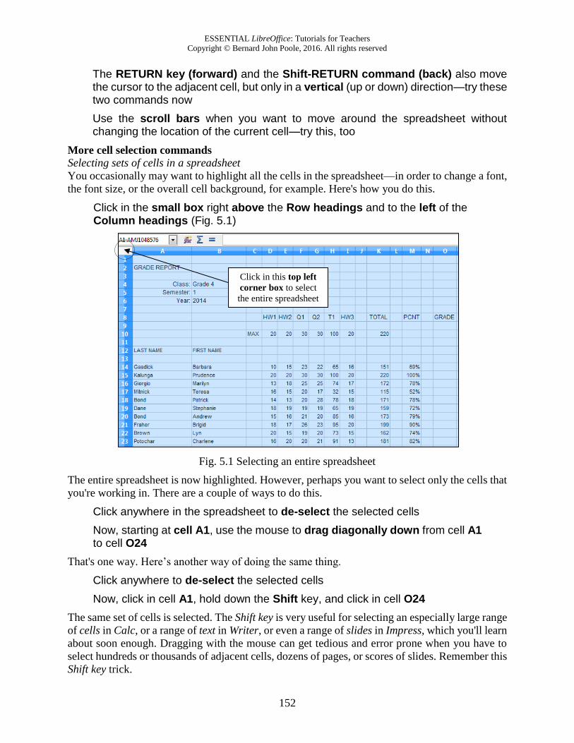
Click in the small box right above the Row headings and to the left of the Column headings (Fig. 5.1)
Fig. 5.1 Selecting an entire spreadsheet
The entire spreadsheet is now highlighted. However, perhaps you want to select only the cells that
you're working in. There are a couple of ways to do this.
Click anywhere in the spreadsheet to de-select the selected cells
Now, starting at cell A1, use the mouse to drag diagonally down from cell A1 to cell O24
That's one way. Here’s another way of doing the same thing.
Click anywhere to de-select the selected cells
Now, click in cell A1, hold down the Shift key, and click in cell O24
The same set of cells is selected. The Shift key is very useful for selecting an especially large range
of cells in Calc, or a range of text in Writer, or even a range of slides in Impress, which you'll learn
about soon enough. Dragging with the mouse can get tedious and error prone when you have to
select hundreds or thousands of adjacent cells, dozens of pages, or scores of slides. Remember this
Shift key trick.
Click in this top left
corner box to select
the entire spreadsheet

Lesson 5: More on the Use of the Spreadsheet
153
Going to a specific cell anywhere in a spreadsheet
If you are working in a large spreadsheet (consisting of thousands of cells, say) and you know the
approximate coordinates of a cell you want to find, it is sometimes quicker to let Calc find the cell
for you. The following simple steps will show you how to make the cell that intersects Column AJ
and Row 423—a location quite deep inside the spreadsheet—the current (or selected) cell.
Click again in the small box right above the Row headings and to the left of the Column headings (Fig. 5.1 on the previous page), type AJ423 (you can use either upper case (AJ) or lower case (aj) for the column coordinate), then click on OK
There you go! Remember that the first (alphabetic) coordinate (AJ) is always the column; the
second (numerical) coordinate is always the Row.
Click again in the small box right above the Row headings and to the left of the Column headings (Fig. 5.1 on the previous page), then type A1, and click on OK
You are now back at the first cell (A1) in the spreadsheet. Some of the options for moving about
the spreadsheet are considerably slower than others, which is why you should take the time to
familiarize yourself with all the different methods for moving around the spreadsheet, especially
if you become a regular user of Calc.
5.3 UPDATING AN EXISTING SPREADSHEET The Gradebook document would benefit from some cosmetic changes, such as the following.
1. There should be double lines to set off different parts of the spreadsheet. It is often useful, for
example, to include extra space (but not too much space) between the headings above the
columns of data and the data itself, and also before summary totals at the bottom of columns
of data.
2. It would be useful to include more formulas to increase the information content of the
spreadsheet. For example, you could add a formula that calculates an average for each of the
sets of grades so that your students can see where they stand in relation to the rest of the class
on any particular assignment or test. A highest score and lowest score for each set of grades
would also be useful.
3. It would be a good idea to protect cells containing data that you consider especially important.
Protecting cells prevents you or someone else from accidentally losing or changing cell
contents. It takes time to put together spreadsheet templates and other documents. Some cells
will contain functions that are tricky to figure out. Protecting them will make it difficult to
lose your work.
4. Finally, Calc can do some of the thinking for you if you include a LOOKUP Table to figure
out the Letter grades for your students based on their percentage score at the end of a reporting
period.
Let's deal with these problems one at a time. In this section you'll learn how to handle the first
three improvements. Later in the lesson you’ll have the opportunity to learn how to create and use
the LOOKUP function.
ESSENTIAL LibreOffice: Tutorials for Teachers
Copyright © Bernard John Poole, 2016. All rights reserved
154
Dividing up the spreadsheet to make it easier to read
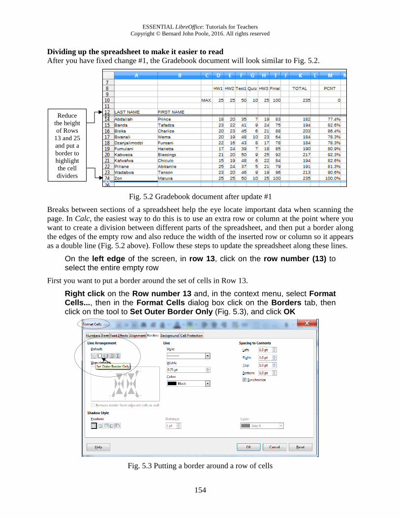
After you have fixed change #1, the Gradebook document will look similar to Fig. 5.2.
Fig. 5.2 Gradebook document after update #1
Breaks between sections of a spreadsheet help the eye locate important data when scanning the
page. In Calc, the easiest way to do this is to use an extra row or column at the point where you
want to create a division between different parts of the spreadsheet, and then put a border along
the edges of the empty row and also reduce the width of the inserted row or column so it appears
as a double line (Fig. 5.2 above). Follow these steps to update the spreadsheet along these lines.
On the left edge of the screen, in row 13, click on the row number (13) to select the entire empty row
First you want to put a border around the set of cells in Row 13.
Right click on the Row number 13 and, in the context menu, select Format Cells..., then in the Format Cells dialog box click on the Borders tab, then click on the tool to Set Outer Border Only (Fig. 5.3), and click OK
Fig. 5.3 Putting a border around a row of cells
Reduce
the height
of Rows
13 and 25
and put a
border to
highlight
the cell
dividers
Lesson 5: More on the Use of the Spreadsheet
155
Now you want to reduce the row height so the whole row looks like a double line separating Rows
12 and 14.
Right click again on the Row Number 13 and, in the context menu, select Row Height..., then in the Row Height dialog box type the value 0.05” to replace the default height, and click OK
You need to create a similar dividing line after Row 24, which holds the data for the last student
in the roster. This is because you are shortly going to include new formulas in Rows 26 thru 28.
Right click on the Row number 26 and, in the context menu, select Format Cells..., then in the Format Cells dialog box click on the Borders tab, then click on the Set outer border only tool (Fig. 5.3 previous page), and click OK
Right click again on the Row Number 26 and, in the context menu, select Row Height..., then in the Row Height dialog box type the value 0.05” to replace the default height, in the Shadow style section click on the first (no shadow) button, and click OK, then save your work (Ctrl+s)
Adding functions to the spreadsheet
As you learned in Lesson 4, Calc comes with many built-in functions for the spreadsheet. Let’s
look at some of the built-in functions so that you know how to find them when you need them.
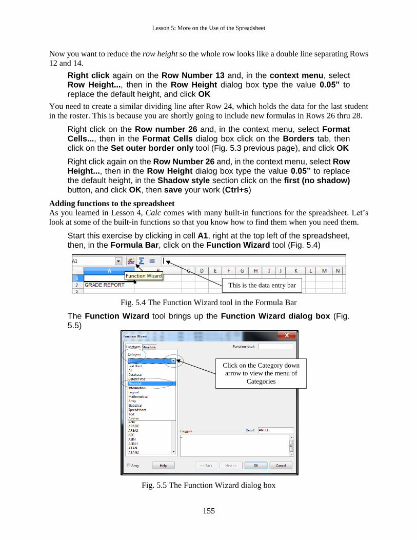
Start this exercise by clicking in cell A1, right at the top left of the spreadsheet, then, in the Formula Bar, click on the Function Wizard tool (Fig. 5.4)
Fig. 5.4 The Function Wizard tool in the Formula Bar
The Function Wizard tool brings up the Function Wizard dialog box (Fig. 5.5)
Fig. 5.5 The Function Wizard dialog box
This is the data entry bar
Click on the Category down
arrow to view the menu of
Categories
ESSENTIAL LibreOffice: Tutorials for Teachers
Copyright © Bernard John Poole, 2016. All rights reserved
156
In the Category section, click on the down arrow to bring up the various Categories of Functions available in LibreOffice (Fig. 5.5 previous page) and select the Financial category, then, in the Function section of the dialog box, check out the several dozen Financial functions available to you there
Do the same with the Calc Database, Date&Time, Information, Logical, Mathematical, Statistical, Spreadsheet, and Text sets of built-in Functions
If you’re feeling overwhelmed, relax. Complete the exercises that follow and you’ll start to get the
hang of using functions such as these.
Click on the Cancel button to close the Function Wizard dialog box
Experience is the best way to learn how some of these functions work. In Lesson 4 you already
learned to use the Sum function, and also you created your own formula to calculate the Percentage
for each student.
You are going to add three new functions to the Gradebook document: the Average, the Max,
and the Min functions. Let’s start with the Average function, which will calculate the average
score for a set of student scores.
Calculating an average for each of the Grade columns
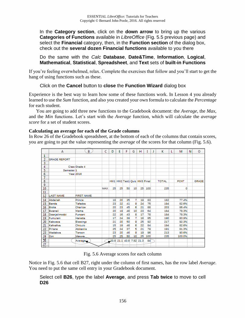
In Row 26 of the Gradebook spreadsheet, at the bottom of each of the columns that contain scores,
you are going to put the value representing the average of the scores for that column (Fig. 5.6).
Fig. 5.6 Average scores for each column
Notice in Fig. 5.6 that cell B27, right under the column of first names, has the row label Average.
You need to put the same cell entry in your Gradebook document.
Select cell B26, type the label Average, and press Tab twice to move to cell D26
Lesson 5: More on the Use of the Spreadsheet
157
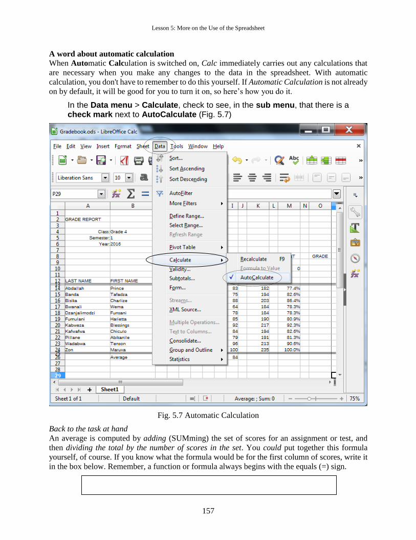
A word about automatic calculation
When Automatic Calculation is switched on, Calc immediately carries out any calculations that
are necessary when you make any changes to the data in the spreadsheet. With automatic
calculation, you don't have to remember to do this yourself. If Automatic Calculation is not already
on by default, it will be good for you to turn it on, so here’s how you do it.
In the Data menu > Calculate, check to see, in the sub menu, that there is a check mark next to AutoCalculate (Fig. 5.7)
Fig. 5.7 Automatic Calculation
Back to the task at hand
An average is computed by adding (SUMming) the set of scores for an assignment or test, and
then dividing the total by the number of scores in the set. You could put together this formula
yourself, of course. If you know what the formula would be for the first column of scores, write it
in the box below. Remember, a function or formula always begins with the equals (=) sign.
ESSENTIAL LibreOffice: Tutorials for Teachers
Copyright © Bernard John Poole, 2016. All rights reserved
158
Check the footnote below to see if you got the answer right1. Since Calc has a built-in Average
function, you may as well use it. Here are the steps to include the Average function in your
spreadsheet.
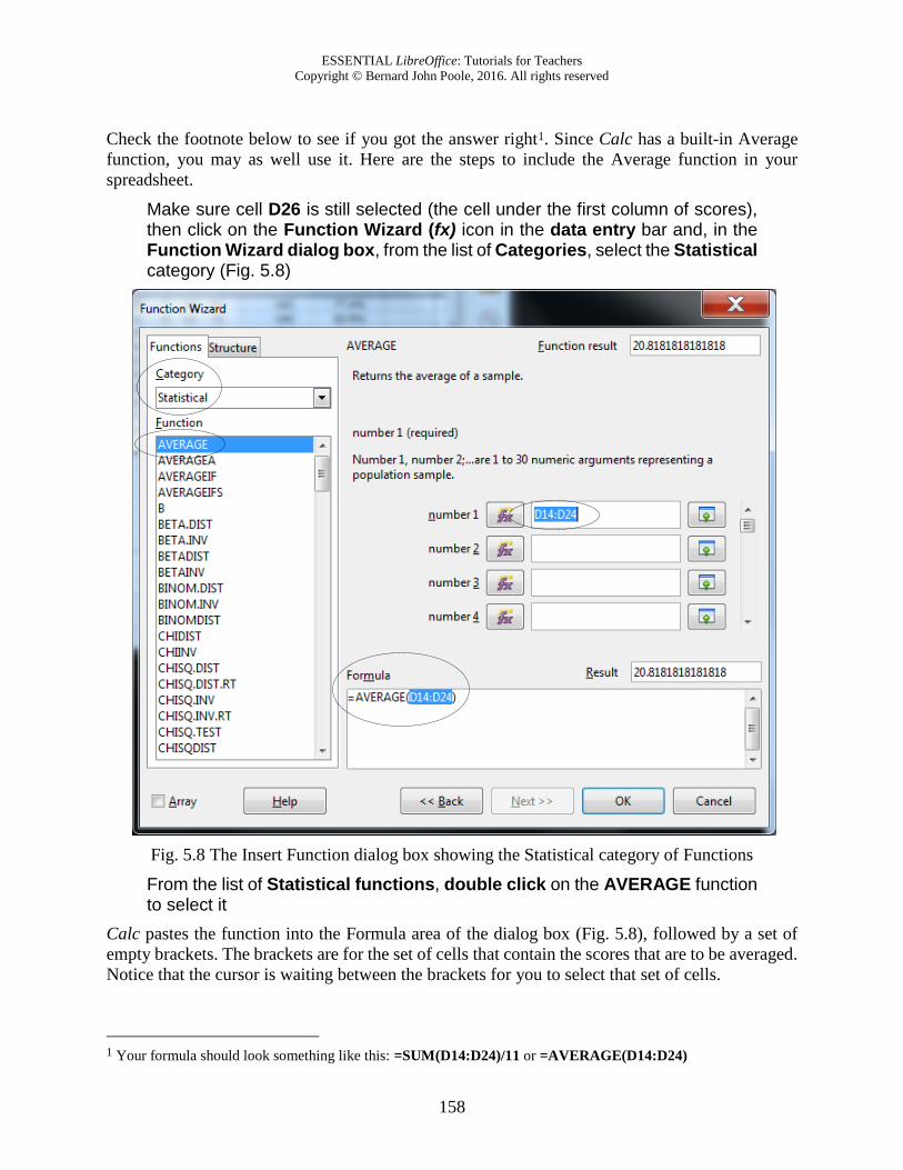
Make sure cell D26 is still selected (the cell under the first column of scores), then click on the Function Wizard (fx) icon in the data entry bar and, in the Function Wizard dialog box, from the list of Categories, select the Statistical category (Fig. 5.8)
Fig. 5.8 The Insert Function dialog box showing the Statistical category of Functions
From the list of Statistical functions, double click on the AVERAGE function to select it
Calc pastes the function into the Formula area of the dialog box (Fig. 5.8), followed by a set of
empty brackets. The brackets are for the set of cells that contain the scores that are to be averaged.
Notice that the cursor is waiting between the brackets for you to select that set of cells.
1 Your formula should look something like this: =SUM(D14:D24)/11 or =AVERAGE(D14:D24)
Lesson 5: More on the Use of the Spreadsheet
159
Type D14:24 (Fig. 5.8 above) or use the mouse to drag, in column B, from cell B14 to cell B24, then click on OK
Look at the data entry bar at the top of the spreadsheet and notice that the formula =AVERAGE
(D14:D24) is copied there, too.
Now look at cell D26. It should contain the average for the scores in Column D. At this
stage there are three problems that can occur:
1. If you see a series of pound signs (###), this tells you there’s not enough room in the column
to show the value, so you might need to widen the column a little to make enough space for
the average score to appear. If this is the case (where you see ### instead of an average score),
make the column wider (Right click on the column header > Column Width…).
2. If a Bad Formula prompt pops up on the screen, check your formula in the entry bar again,
compare it to the correct Average formula =AVERAGE(D14:D24), and make any corrections.
3. It is always possible that the values being averaged yield a result that turns out to be a whole
number (no fractions). But it would be useful to show at least one decimal place, regardless
of the outcome of the Average calculation. Here are the steps to change the precision of the
Average value to 1 decimal place.
Cell D26 should still be selected (click on it if it is not selected)
In the Format menu select Cells… > Numbers tab and, in the Options area, set the number of Decimal places to 1
Assuming all is well, your next task will be to copy this Average formula into the cells immediately
to the right of cell D26, so that you have an average score under the other columns of scores (cells
E26 through I26).
Cell D26 should still be selected (click on it if it is not selected)
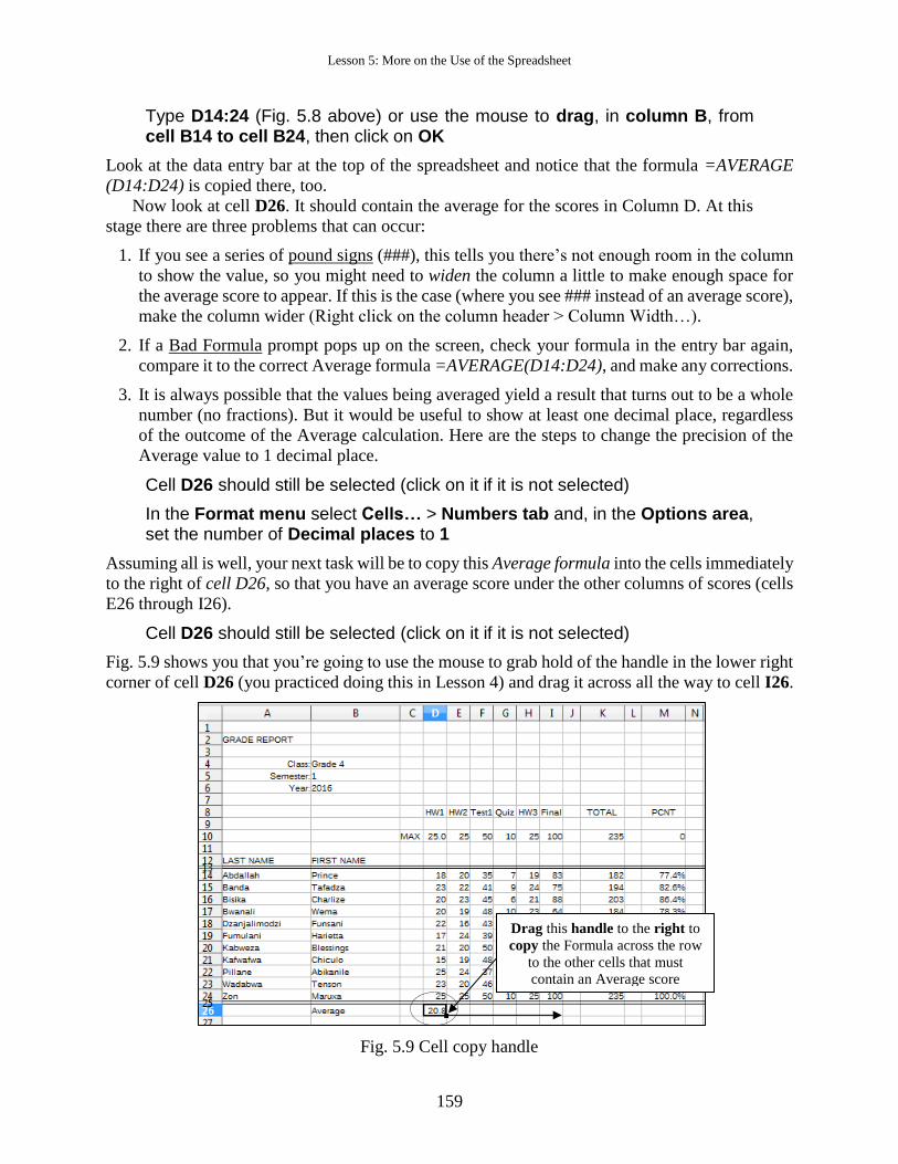
Fig. 5.9 shows you that you’re going to use the mouse to grab hold of the handle in the lower right
corner of cell D26 (you practiced doing this in Lesson 4) and drag it across all the way to cell I26.
Fig. 5.9 Cell copy handle
Drag this handle to the right to
copy the Formula across the row
to the other cells that must
contain an Average score

ESSENTIAL LibreOffice: Tutorials for Teachers
Copyright © Bernard John Poole, 2016. All rights reserved
160
Use the mouse to point at the handle in the lower right corner of cell D26 (Fig. 5.9), and drag the handle across to Column I, cell I26—so that the formula is copied across to cells E26, F26, G26, H26, and I26, which will all now have the correct Average score for their respective columns
That's all there is to it. If necessary (though it shouldn’t be the case with this exercise) adjust the
column widths if you see pound signs (###) in any cell instead of averages.
Time to save all your hard work (Ctrl+s)
Displaying the Highest (MAX) and Lowest (MIN) scores for each column of scores
Now that you know how to use the Insert Function icon (fx) next to the Data Entry bar, and in
particular since you just used it to put the Average function in your spreadsheet, you should be
able to complete the exercise that follows without much help.
In cell B27 put the heading Max score and in cell B28 put the heading Min score
Make sure cell D27 is selected (the cell under the first Average calculation), then click on the Function Wizard (fx) icon in the data entry bar and, in the Function Wizard dialog box, from the list of Categories, select the Statistical category (Fig. 5.8 on page 158)
From the list of Statistical functions, double click on the MAX function to select it
Calc again pastes the function into the Formula area of the dialog box, followed by a set of empty
brackets. The brackets are for the set of cells that contain the scores that are to be averaged. Notice
that the cursor is waiting between the brackets for you to select that set of cells.
Type D14:D24 (Fig. 5.8 again—p. 158) then click on OK
Look at the data entry bar at the top of the spreadsheet and notice that the formula =MAX
(D14:D24) is copied there, too. Now look at cell D27. It should contain the maximum score in
Column D. Check to confirm that that is indeed the case.
You should be starting to feel comfortable building functions in the spreadsheet.
Now make sure cell D28 is selected (the cell where you’re going to put the MIN formula), then click on the Function Wizard (fx) icon in the data entry bar and, in the Function Wizard dialog box, from the list of Categories, select the Statistical category (Fig. 5.8 on page 148)
From the list of Statistical functions, double click on the MIN function to select it
Calc again pastes the function into the Formula area of the dialog box, followed by a set of empty
brackets. As you now know, the brackets are for the set of cells that contain the scores that are to
be averaged. Notice again that the cursor is waiting between the brackets for you to select that set
of cells.
Type D14:D24 (Fig. 5.8—p. 148) then click on OK
Lesson 5: More on the Use of the Spreadsheet
161
Look at the data entry bar at the top of the spreadsheet and notice that the formula =MIN
(D14:D24) is copied there, too. Now look at cell D27. It should contain the maximum score in
Column D. Check to confirm that that is indeed the case.
At this stage, the last task is to copy the MIN and MAX Functions across to the other cells in
rows 27 and 28. You probably already know how to do this, but here are the steps in case you need
help.
With cell D26 selected, grab hold of the handle in the lower right corner of the cell and drag across with the mouse to select cells E26 through I26—the cells in which you want to include the Max function, and click OK
Uh oh; cell I27 may not be wide enough for the highest possible value in the Max score row
(100.0%). It’s possible a student could have that score, so you’ll need to widen Column I so the
data can fit in the cell.
Right click on the Column header (I) at the top of the column and, in the context menu, select Column Width…, then in the dialog box type 0.50” and click on OK
Now, with cell D28 selected, grab hold of the handle in the lower right corner of the cell and drag across with the mouse to select cells E27 through I27—the cells in which you want to include the Min function, and click OK
Better Save your work (Ctrl+s)
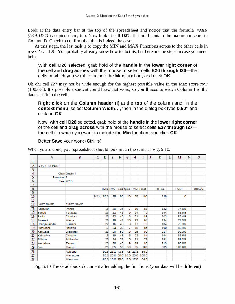
When you're done, your spreadsheet should look much the same as Fig. 5.10.
Fig. 5.10 The Gradebook document after adding the functions (your data will be different)
ESSENTIAL LibreOffice: Tutorials for Teachers
Copyright © Bernard John Poole, 2016. All rights reserved
162
Protecting (locking) important cells
Calc allows you to protect the contents of a cell or cells. This means that neither you nor anyone
else will be able to change the contents unless you remove the protection. This feature is useful to
prevent accidental loss of data, and will also help prevent others from interfering with the data you
have collected.
Since all the data in a Grade book are important, it would be a good idea to protect everything.
The process to do this is the same as if you were protecting a single cell, or a few cells, except that
you select every cell.
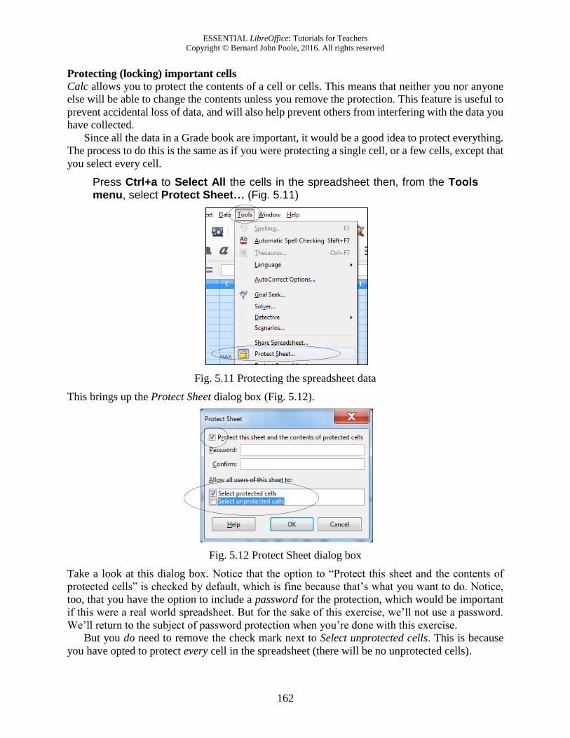
Press Ctrl+a to Select All the cells in the spreadsheet then, from the Tools menu, select Protect Sheet… (Fig. 5.11)
Fig. 5.11 Protecting the spreadsheet data
This brings up the Protect Sheet dialog box (Fig. 5.12).
Fig. 5.12 Protect Sheet dialog box
Take a look at this dialog box. Notice that the option to “Protect this sheet and the contents of
protected cells” is checked by default, which is fine because that’s what you want to do. Notice,
too, that you have the option to include a password for the protection, which would be important
if this were a real world spreadsheet. But for the sake of this exercise, we’ll not use a password.
We’ll return to the subject of password protection when you’re done with this exercise.
But you do need to remove the check mark next to Select unprotected cells. This is because
you have opted to protect every cell in the spreadsheet (there will be no unprotected cells).
Lesson 5: More on the Use of the Spreadsheet
163
So, click to remove the check mark/tick next to Select unprotected cells, then click on OK
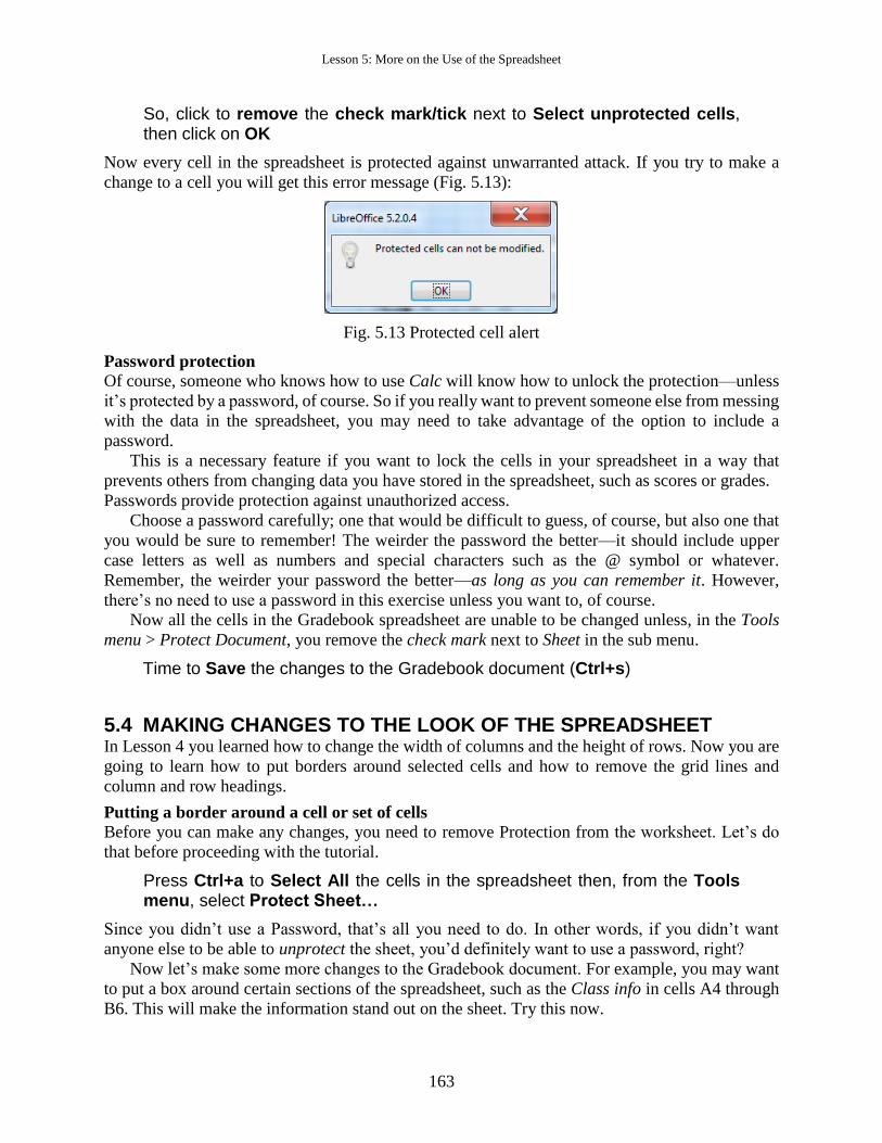
Now every cell in the spreadsheet is protected against unwarranted attack. If you try to make a
change to a cell you will get this error message (Fig. 5.13):
Fig. 5.13 Protected cell alert
Password protection
Of course, someone who knows how to use Calc will know how to unlock the protection—unless
it’s protected by a password, of course. So if you really want to prevent someone else from messing
with the data in the spreadsheet, you may need to take advantage of the option to include a
password.
This is a necessary feature if you want to lock the cells in your spreadsheet in a way that
prevents others from changing data you have stored in the spreadsheet, such as scores or grades.
Passwords provide protection against unauthorized access.
Choose a password carefully; one that would be difficult to guess, of course, but also one that
you would be sure to remember! The weirder the password the better—it should include upper
case letters as well as numbers and special characters such as the @ symbol or whatever.
Remember, the weirder your password the better—as long as you can remember it. However,
there’s no need to use a password in this exercise unless you want to, of course.
Now all the cells in the Gradebook spreadsheet are unable to be changed unless, in the Tools
menu > Protect Document, you remove the check mark next to Sheet in the sub menu.
Time to Save the changes to the Gradebook document (Ctrl+s)
5.4 MAKING CHANGES TO THE LOOK OF THE SPREADSHEET In Lesson 4 you learned how to change the width of columns and the height of rows. Now you are
going to learn how to put borders around selected cells and how to remove the grid lines and
column and row headings.
Putting a border around a cell or set of cells
Before you can make any changes, you need to remove Protection from the worksheet. Let’s do
that before proceeding with the tutorial.
Press Ctrl+a to Select All the cells in the spreadsheet then, from the Tools menu, select Protect Sheet…
Since you didn’t use a Password, that’s all you need to do. In other words, if you didn’t want
anyone else to be able to unprotect the sheet, you’d definitely want to use a password, right?
Now let’s make some more changes to the Gradebook document. For example, you may want
to put a box around certain sections of the spreadsheet, such as the Class info in cells A4 through
B6. This will make the information stand out on the sheet. Try this now.
ESSENTIAL LibreOffice: Tutorials for Teachers
Copyright © Bernard John Poole, 2016. All rights reserved
164
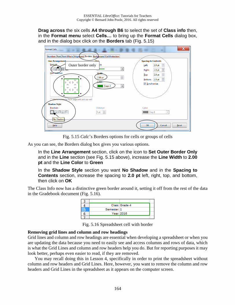
Drag across the six cells A4 through B6 to select the set of Class info then, in the Format menu select Cells… to bring up the Format Cells dialog box, and in the dialog box click on the Borders tab (Fig. 5.15)
Fig. 5.15 Calc’s Borders options for cells or groups of cells
As you can see, the Borders dialog box gives you various options.
In the Line Arrangement section, click on the icon to Set Outer Border Only and in the Line section (see Fig. 5.15 above), increase the Line Width to 2.00 pt and the Line Color to Green
In the Shadow Style section you want No Shadow and in the Spacing to Contents section, increase the spacing to 2.0 pt left, right, top, and bottom, then click on OK
The Class Info now has a distinctive green border around it, setting it off from the rest of the data
in the Gradebook document (Fig. 5.16).
Fig. 5.16 Spreadsheet cell with border
Removing grid lines and column and row headings
Grid lines and column and row headings are essential when developing a spreadsheet or when you
are updating the data because you need to easily see and access columns and rows of data, which
is what the Grid Lines and column and row headers help you do. But for reporting purposes it may
look better, perhaps even easier to read, if they are removed.
You may recall doing this in Lesson 4, specifically in order to print the spreadsheet without
column and row headers and Grid Lines. Here, however, you want to remove the column and row
headers and Grid Lines in the spreadsheet as it appears on the computer screen.
Outer border only
Lesson 5: More on the Use of the Spreadsheet
165
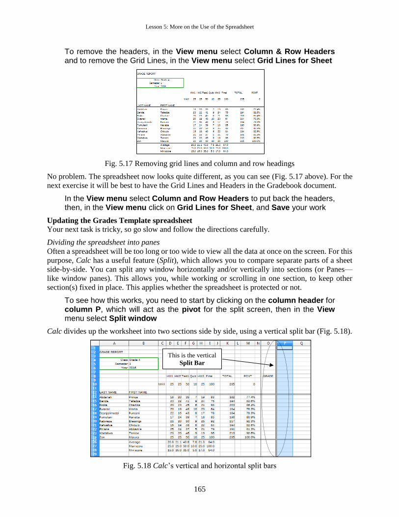
To remove the headers, in the View menu select Column & Row Headers and to remove the Grid Lines, in the View menu select Grid Lines for Sheet
Fig. 5.17 Removing grid lines and column and row headings
No problem. The spreadsheet now looks quite different, as you can see (Fig. 5.17 above). For the
next exercise it will be best to have the Grid Lines and Headers in the Gradebook document.
In the View menu select Column and Row Headers to put back the headers, then, in the View menu click on Grid Lines for Sheet, and Save your work
Updating the Grades Template spreadsheet
Your next task is tricky, so go slow and follow the directions carefully.
Dividing the spreadsheet into panes
Often a spreadsheet will be too long or too wide to view all the data at once on the screen. For this
purpose, Calc has a useful feature (Split), which allows you to compare separate parts of a sheet
side-by-side. You can split any window horizontally and/or vertically into sections (or Panes—
like window panes). This allows you, while working or scrolling in one section, to keep other
section(s) fixed in place. This applies whether the spreadsheet is protected or not.
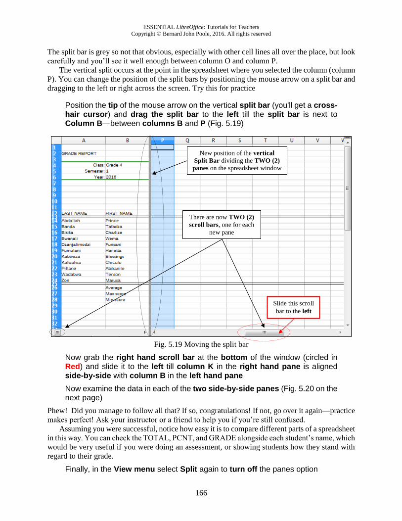
To see how this works, you need to start by clicking on the column header for column P, which will act as the pivot for the split screen, then in the View menu select Split window
Calc divides up the worksheet into two sections side by side, using a vertical split bar (Fig. 5.18).
Fig. 5.18 Calc’s vertical and horizontal split bars
This is the vertical
Split Bar
ESSENTIAL LibreOffice: Tutorials for Teachers
Copyright © Bernard John Poole, 2016. All rights reserved
166
The split bar is grey so not that obvious, especially with other cell lines all over the place, but look
carefully and you’ll see it well enough between column O and column P.
The vertical split occurs at the point in the spreadsheet where you selected the column (column
P). You can change the position of the split bars by positioning the mouse arrow on a split bar and
dragging to the left or right across the screen. Try this for practice
Position the tip of the mouse arrow on the vertical split bar (you'll get a cross-hair cursor) and drag the split bar to the left till the split bar is next to Column B—between columns B and P (Fig. 5.19)
Fig. 5.19 Moving the split bar
Now grab the right hand scroll bar at the bottom of the window (circled in Red) and slide it to the left till column K in the right hand pane is aligned side-by-side with column B in the left hand pane
Now examine the data in each of the two side-by-side panes (Fig. 5.20 on the next page)
Phew! Did you manage to follow all that? If so, congratulations! If not, go over it again—practice
makes perfect! Ask your instructor or a friend to help you if you’re still confused.
Assuming you were successful, notice how easy it is to compare different parts of a spreadsheet
in this way. You can check the TOTAL, PCNT, and GRADE alongside each student’s name, which
would be very useful if you were doing an assessment, or showing students how they stand with
regard to their grade.
Finally, in the View menu select Split again to turn off the panes option
New position of the vertical
Split Bar dividing the TWO (2)
panes on the spreadsheet window
There are now TWO (2)
scroll bars, one for each
new pane
Slide this scroll
bar to the left
Lesson 5: More on the Use of the Spreadsheet
167
Fig. 5.20 Comparing Student Names with the summary data
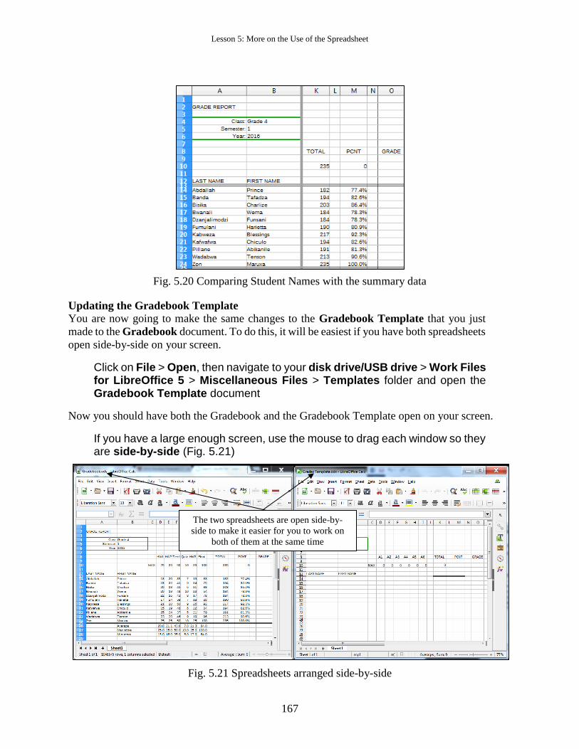
Updating the Gradebook Template
You are now going to make the same changes to the Gradebook Template that you just
made to the Gradebook document. To do this, it will be easiest if you have both spreadsheets
open side-by-side on your screen.
Click on File > Open, then navigate to your disk drive/USB drive > Work Files for LibreOffice 5 > Miscellaneous Files > Templates folder and open the Gradebook Template document
Now you should have both the Gradebook and the Gradebook Template open on your screen.
If you have a large enough screen, use the mouse to drag each window so they are side-by-side (Fig. 5.21)
Fig. 5.21 Spreadsheets arranged side-by-side
The two spreadsheets are open side-by-
side to make it easier for you to work on
both of them at the same time
ESSENTIAL LibreOffice: Tutorials for Teachers
Copyright © Bernard John Poole, 2016. All rights reserved
168
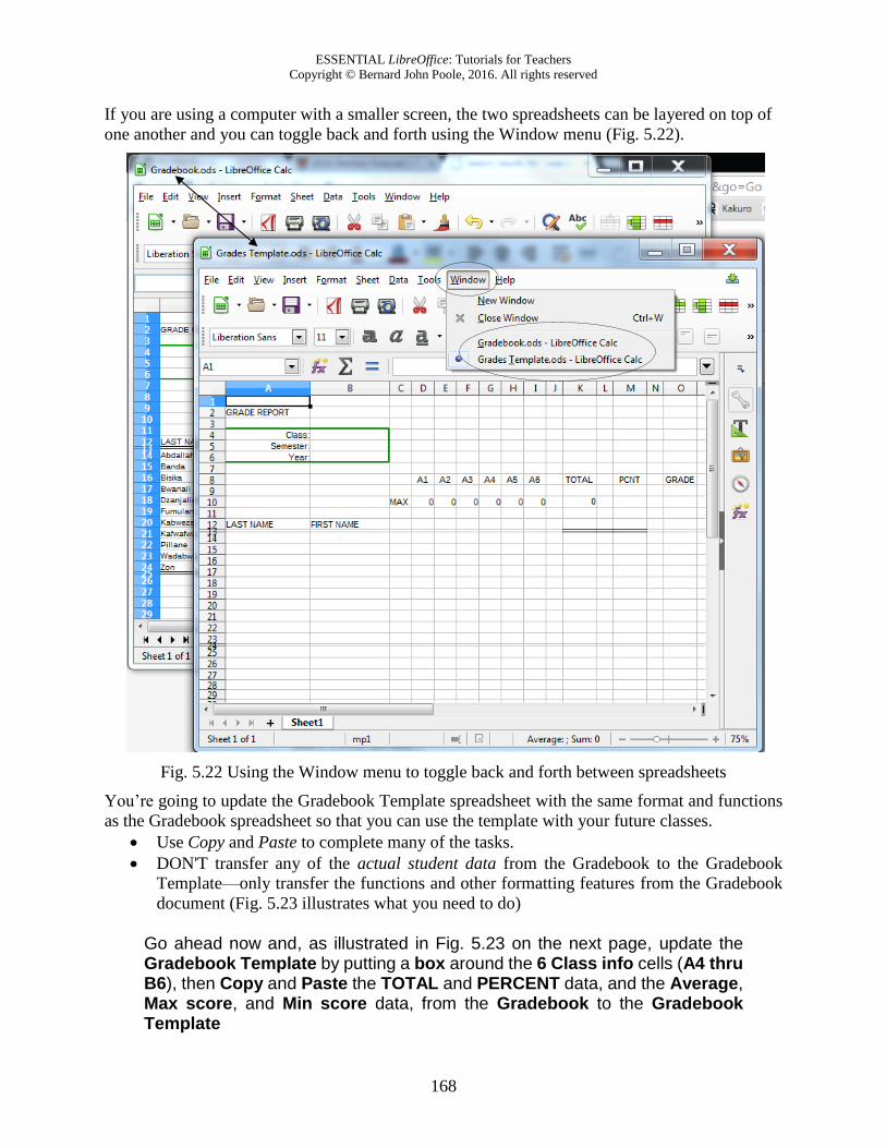
If you are using a computer with a smaller screen, the two spreadsheets can be layered on top of
one another and you can toggle back and forth using the Window menu (Fig. 5.22).
Fig. 5.22 Using the Window menu to toggle back and forth between spreadsheets
You’re going to update the Gradebook Template spreadsheet with the same format and functions
as the Gradebook spreadsheet so that you can use the template with your future classes.
Use Copy and Paste to complete many of the tasks.
DON'T transfer any of the actual student data from the Gradebook to the Gradebook
Template—only transfer the functions and other formatting features from the Gradebook
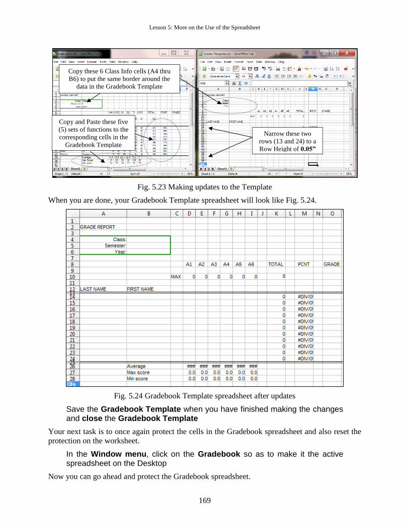
document (Fig. 5.23 illustrates what you need to do) Go ahead now and, as illustrated in Fig. 5.23 on the next page, update the Gradebook Template by putting a box around the 6 Class info cells (A4 thru B6), then Copy and Paste the TOTAL and PERCENT data, and the Average, Max score, and Min score data, from the Gradebook to the Gradebook Template
Lesson 5: More on the Use of the Spreadsheet
169
Fig. 5.23 Making updates to the Template
When you are done, your Gradebook Template spreadsheet will look like Fig. 5.24.
Fig. 5.24 Gradebook Template spreadsheet after updates
Save the Gradebook Template when you have finished making the changes and close the Gradebook Template
Your next task is to once again protect the cells in the Gradebook spreadsheet and also reset the
protection on the worksheet.
In the Window menu, click on the Gradebook so as to make it the active spreadsheet on the Desktop
Now you can go ahead and protect the Gradebook spreadsheet.
Narrow these two
rows (13 and 24) to a
Row Height of 0.05”
Copy and Paste these five
(5) sets of functions to the
corresponding cells in the
Gradebook Template
Copy these 6 Class Info cells (A4 thru
B6) to put the same border around the
data in the Gradebook Template
spreadsheet

ESSENTIAL LibreOffice: Tutorials for Teachers
Copyright © Bernard John Poole, 2016. All rights reserved
170
Press Ctrl+a to Select All the cells in the spreadsheet (this is the quickest way to select all the cells in the spreadsheet, but you may recall that you can also click in the small box in the top left corner of the row and column headings)
From the Tools menu select Protect Sheet…
In the Protect Sheet dialog box that pops up, click to remove the check mark/tick next to Select unprotected cells (see Fig. 5.12 on page 162) then click on OK, and Save your work
It might be a good idea to take a break at this point in the tutorial. But if you feel up to it, feel free
to proceed directly to the next section, Section 5.5 on the next page.
TIME FOR A BREAK?
FEEL FREE TO TAKE ONE…
THIS MIGHT BE ENOUGH FOR ONE DAY!
Lesson 5: More on the Use of the Spreadsheet
171
5.5 USING THE LOOKUP FUNCTION The concept of the LOOKUP function
The spreadsheet LOOKUP function is a little tricky to understand, so stand up, step back from the
keyboard for a while and stretch some of those muscles that are stiff from sitting through the first
part of this tutorial. When you are ready, read quietly through this section to understand how the
LOOKUP function works.
The LOOKUP function is a simple logic tool that you can use to automatically assign grades
to your students based on the numbers in the Percentage column of your spreadsheet (column L).
You are probably aware by now that if you have the automatic calculation option selected,
Calc carries out function-based calculations as you make changes in a spreadsheet. Thus, once you
have programmed Calc to LOOKUP the grades, the system will automatically update each
student's Letter Grade, along with Totals and Percentages, even as you enter new scores for
assignments, homework, tests, and so forth.
Thus, with no effort on your part, you will be able to keep students informed at any time during
the semester as to exactly what grade they currently carry for the class.
Such information is invaluable. Knowledge is power. When a student is aware of an inadequate
grade early on, extra effort can be applied to improve the situation before it is too late. It is
surprising how often students are unaware of how they stand with regard to their progress through
a course. The teacher who fails to provide adequate feedback when directing students in their
pursuit of academic objectives deserves at least some of the blame if students do not progress as
well as they should. When students are kept apprised at all times of where they stand they tend to
take more responsibility for the outcomes of their efforts—or lack of them.
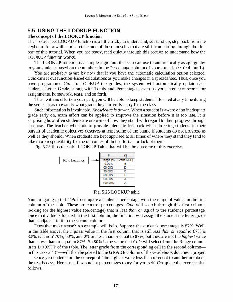
Fig. 5.25 illustrates the LOOKUP Table that will be the outcome of this exercise.
Fig. 5.25 LOOKUP table
You are going to tell Calc to compare a student's percentage with the range of values in the first
column of the table. These are control percentages. Calc will search through this first column,
looking for the highest value (percentage) that is less than or equal to the student's percentage.
Once that value is located in the first column, the function will assign the student the letter grade
that is adjacent to it in the second column.
Does that make sense? An example will help. Suppose the student's percentage is 87%. Well,
in the table above, the highest value in the first column that is still less than or equal to 87% is
80%, is it not? 70%, 60%, and 0% are less than or equal to 87%, but they are not the highest value
that is less than or equal to 87%. So 80% is the value that Calc will select from the Range column
in its LOOKUP of the table. The letter grade from the corresponding cell in the second column—
in this case a "B"—will then be posted to the GRADE column of the Gradebook document proper.
Once you understand the concept of "the highest value less than or equal to another number",
the rest is easy. Here are a few student percentages to try for yourself. Complete the exercise that
follows.
Row headings
ESSENTIAL LibreOffice: Tutorials for Teachers
Copyright © Bernard John Poole, 2016. All rights reserved
172
From Fig. 5.25, column 1,
What is the highest value less than or equal to 45%, and what is the resulting letter grade?_____________
What is the highest value less than or equal to 67%, and what is the resulting letter grade?_____________
What is the highest value less than or equal to 59%, and what is the resulting letter grade?_____________
What is the highest value less than or equal to 100%, and what’s the resulting letter grade?_____________
The answers are in the footnote at the bottom of the page.1
There are two parts to incorporating the Calc LOOKUP function into your Gradebook document.
First you must build the LOOKUP Table into the spreadsheet. Second you must enter into the
appropriate cells the LOOKUP function that will instruct Calc to carry out the LOOKUP operation.
Building the LOOKUP Table
You’ll need both the Gradebook document (which you saved in the Data Files folder in the Spreadsheet Documents folder) and the Gradebook Template (which you also saved in the Data Files folder in the Spreadsheet Documents folder) to complete the remainder of this tutorial, so if these documents are not already open, open them both from your Work Files for LibreOffice 5 folder before proceeding
Next, in the Window menu select the Gradebook document, if it is not already the active window on the screen
Since all the cells are protected in the Gradebook document, you’ll need to unlock them first in
order to make changes.
From the Tools menu select Protect Sheet… to toggle the protection off
Now you’ll be able to work with the data in the spreadsheet. Let’s build the Lookup table that’s
illustrated in Fig. 5.25 above (page 171). The first column of the LOOKUP Table (the lookup
vector) has a set of numbers which Calc calls the Search vector.
A vector is just another name for a single column of numbers. The Search vector contains the
set of values against which Calc compares the data from a selected cell in the Gradebook
document.
Let’s create this column (vector) of the LOOKUP table first. As you work your way through
this exercise, be sure to hit the number 0, NOT the letter O; they are so close together on the
keyboard that some students hit the wrong character by mistake.
Select cell P1 and type the column header Range (%) then press Enter to move down to cell P2
Type 0 (the number zero (0) that is) in cell P2 and press Enter to move down to cell P3
Type 0.6 (this is equivalent to 60% in mathematical terms) and press Enter again to select cell P4
1 0% (E); 60% (D); 0% (E); 100% (A)
Lesson 5: More on the Use of the Spreadsheet
173
Type 0.7 and press Enter to make P5 the current cell
Type 0.8 and press Enter once more
Type 0.9 in cell P6 and press Enter again to make PrANGE (%)7 the current cell
Finally type 1 (this is equivalent to 100% in mathematical terms) and click on the Accept ( ) button
Now you must change the cell attributes of this first column of the table so as to display the
numbers in percent form (with the percent (%) symbol). You did this before in Lesson 4, so the
following is just a reminder of how to do this.
Drag down to highlight all 6 of the scale values from cell P2 to cell P7
In the Formatting toolbar click on the % (Percent) symbol to change the format of the decimal numbers to percentages
If the percentages have decimal places, right click on the column of selected percentages
In the context menu that pops up, select Format Cells… to bring up the Format Cells dialog box, click on the Numbers tab and then, in the Options section, make sure the Decimal places option is set to 0 (zero)
That completes the first column of the table. Now for the second column with the letter grades—
what Calc calls the result vector. The result vector contains the values which Calc returns to the
Gradebook cell which contains the formula which calls on the LOOKUP function.
Select cell Q1 and type the header Grade (A-E), then press Enter to move down to cell Q2
Type the letter E (or whatever you would use for a failing grade) and press Enter to go to cell Q3
Type a D and move down to cell Q4, then type a C and move down to cell Q5
Type a B and move on down to cell Q6, then type an A and move down to cell Q7
Finally type an A again in cell Q7 and click on the Accept ( ) button
The table is now almost ready for use. A simple cosmetic adjustment will improve its appearance.
Select columns P and Q by dragging across the column headers P and Q at the top of the columns and, in the formatting toolbar, click on the center alignment tool
Your LOOKUP Table should now look like Fig. 5.25 on page 171.
Save all your hard work before proceeding with the tutorial
Using the clipboard to copy cells from one document to another
Now that you have completed the task of building the LOOKUP Table in the Gradebook document
you should update the Gradebook Template along the same lines. The easiest way to do this is to
ESSENTIAL LibreOffice: Tutorials for Teachers
Copyright © Bernard John Poole, 2016. All rights reserved
174
copy the relevant cells from the Gradebook document into the Gradebook Template document
using Copy and Paste.
First you must copy the relevant cells (those used for the LOOKUP Table) from the Gradebook
document to the clipboard. Here are the steps.
Select cell P1 and drag down diagonally across the LOOKUP Table to cell Q7
Press Ctrl+c to copy the LOOKUP Table to the clipboard
Now switch to the Gradebook Template document by switching windows in the Window menu
In the Gradebook Template, click on cell P1 to make it the current cell
Press Ctrl+v to paste the LOOKUP Table from the clipboard to the Gradebook Template, then Save your work (Ctrl+s) once more
Entering the LOOKUP function into the Grade column
Take a moment to read carefully through the next several paragraphs to help you understand the
next step in using the LOOKUP table.
Recall that the LOOKUP function instructs Calc to look up a table that you have built and
return with a corresponding result to store in the spreadsheet proper. Still confused? Maybe the
following will help you figure it out.
The LOOKUP function has the following parts to it:
=LOOKUP(Search criterion,Search vector,result_vector)
Let’s examine each part of this function in order to understand how it works.
As you know by now, the "=" symbol at the start of the function simply tells Calc that
a function or formula is in the cell, as opposed to ordinary data such as numbers or
labels.
The word LOOKUP tells Calc what task it has to carry out (look something up in a
list).
Search criterion, Search vector, and result_vector are variables (control values) that
Calc uses when it is looking up the table in columns P and Q:
the Search criterion is either a number or text (such as a person's name); this value
will be the "key" that Calc will use as it searches through the cells in the Search
vector or column;
the Search vector is the column of cells that Calc has to check in its lookup of the
table (column P in Fig. 5.25 on page 171);
the result_vector is the column of cells in which Calc will find the result of the
LOOKUP operation (Column P in Fig. 5.25 on page 171).
Still confused? Don’t feel bad; this is definitely tricky stuff. Maybe by working an example you
will better understand how the Lookup function works. It will be easiest for you to follow the next
exercise if you have an actual grade book to work with.
Lesson 5: More on the Use of the Spreadsheet
175
The Gradebook Template and Gradebook spreadsheets should still be open on your screen, so begin by switching back to the Gradebook document (use the Window menu to Switch Windows)
As you follow along, make sure you have at least the LOOKUP Table (columns P and Q) showing
on the screen, as well as columns M thru O of the Gradebook document containing the PCNT and
eventual GRADE data.
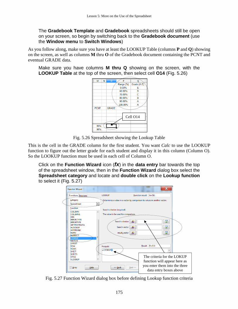
Make sure you have columns M thru Q showing on the screen, with the LOOKUP Table at the top of the screen, then select cell O14 (Fig. 5.26)
Fig. 5.26 Spreadsheet showing the Lookup Table
This is the cell in the GRADE column for the first student. You want Calc to use the LOOKUP
function to figure out the letter grade for each student and display it in this column (Column O).
So the LOOKUP function must be used in each cell of Column O.
Click on the Function Wizard icon (fx) in the data entry bar towards the top
of the spreadsheet window, then in the Function Wizard dialog box select the Spreadsheet category and locate and double click on the Lookup function to select it (Fig. 5.27)
Fig. 5.27 Function Wizard dialog box before defining Lookup function criteria
Cell O14
The criteria for the LOKUP
function will appear here as
you enter them into the three
data entry boxes above
ESSENTIAL LibreOffice: Tutorials for Teachers
Copyright © Bernard John Poole, 2016. All rights reserved
176
Notice in Fig. 5.27 above that the cursor is positioned between the brackets after the word
=LOOKUP (|) in the formula area of the dialog box. The three sets of data for the LOOKUP
function will appear there as you complete the steps that follow.
If the Function Wizard dialog box is covering the cells you need to work with (column M and the Lookup Table in columns P and Q), slide the Function Wizard dialog box down and off to the right or left on the screen so that the dialog box is out of the way
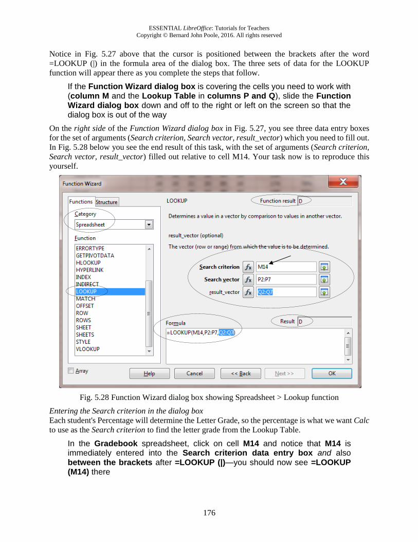
On the right side of the Function Wizard dialog box in Fig. 5.27, you see three data entry boxes
for the set of arguments (Search criterion, Search vector, result_vector) which you need to fill out.
In Fig. 5.28 below you see the end result of this task, with the set of arguments (Search criterion,
Search vector, result_vector) filled out relative to cell M14. Your task now is to reproduce this
yourself.
Fig. 5.28 Function Wizard dialog box showing Spreadsheet > Lookup function
Entering the Search criterion in the dialog box
Each student's Percentage will determine the Letter Grade, so the percentage is what we want Calc
to use as the Search criterion to find the letter grade from the Lookup Table.
In the Gradebook spreadsheet, click on cell M14 and notice that M14 is immediately entered into the Search criterion data entry box and also between the brackets after =LOOKUP (|)—you should now see =LOOKUP (M14) there
Lesson 5: More on the Use of the Spreadsheet
177
So Calc enters this cell's coordinates as the first of the LOOKUP parameters, the Search criterion.
You are telling Calc that it must use this first student's percentage as the value to check against the
first column of the LOOKUP Table (cells P2 through P7).
Entering in the Search vector
Cells P2 through P7 are the Search vector for the LOOKUP Table.
In the Function wizard dialog box, click to position the cursor in the second data entry box—the Search vector entry area (see Fig. 5.28 above)—so you can enter the cells which contain the Search vector
Now, in the Gradebook spreadsheet, use the mouse to drag down from cell P2 to cell P7
Notice that in the data entry bar Calc fills in the second of the LOOKUP parameters for the
LOOKUP function, namely the Search vector. It also appears between the brackets after
=LOOKUP (M14,P2:P7). Check that it also appears in the Gradebook spreadsheet in the Data
entry bar, too. You are almost done with building the LOOKUP function.
Entering the result_vector
Cells Q2 through Q7 are the result_vector for the LOOKUP Table.
Click to put the cursor in the third data entry box so you can specify the cells that contain the result_vector, then, in the Gradebook spreadsheet, drag down from cell Q2 to cell Q7
Notice, once again, that Calc fills in the third of the =LOOKUP (M14,P2:P7,Q2:Q7) parameters,
the result_vector.
In the Gradebook spreadsheet itself, check the data entry bar to see that the LOOKUP function is now complete—at this stage it should read =LOOKUP(M14,P2:P7,Q2:Q7)
Finally, click on OK and Save your work
Applying the function
Calc will look for "the highest value in cells P2 through P7 that is less than or equal to the student's
percentage".
Take a look at cell O14 now and verify that it contains the correct letter grade according to the value in cell M14 (the percentage for this first student)
As you see, once the LOOKUP function has located the correct cell in column 1 of the Lookup
Table (the Range column), all that remains is for Calc to make a note of the letter grade that is in
the corresponding cell in column 2 of the table (the Grade column), and the LOOKUP function
copies that grade into cell O14.
Don’t feel bad if your eyes are starting to glaze over; this is kinda nerdy stuff. But hang in
there, we’re nearly done.
Copying the LOOKUP function into the rest of the GRADE column
The first student's grade is taken care of. The next task is to copy this function from cell O14 down
to the other cells in the GRADE column (column O), but this is not as simple as it seems because
we have to consider the problem of Absolute and Relative cell references.
ESSENTIAL LibreOffice: Tutorials for Teachers
Copyright © Bernard John Poole, 2016. All rights reserved
178
If you want to try and do this on your own (you will need to understand the concept of Absolute
and Relative references!), go ahead. If you are successful you can skip the rest of this sub-section
and go to the Practice makes perfect section on the next page.
If you need help completing the LOOKUP function, read on to follow the steps to correctly
Fill down the LOOKUP function to the remaining cells in column O.
First you must make a small change to the function itself. You also need to put your thinking
cap on, because if this is the first time you've used a LOOKUP function, it can get mighty
confusing.
You may recall learning about Relative and Absolute cell references in Lesson 4. The function
=LOOKUP(L14,P2:P7,Q2:Q7) will work fine for the first student, but if you copy it to the other
cells as is, Calc will assume that all the cell references in the function are relative to the cell into
which they are being copied, and will adjust them accordingly, resulting in the WRONG letter
grades. If you enjoy math or logic, you’ll be enjoying this; but if not, bear with us, OK?
What you have to bear in mind is that the references to the LOOKUP Table (cells P2:P7 and
Q2:Q7) must be absolute references—which means any references to those cells must not
change—because the data for the LOOKUP Table will absolutely always be found in these specific
cells.
So you need to tell Calc to leave these LOOKUP Table references unchanged when copying
the LOOKUP function into the other cells in column N. You do this by surrounding the LOOKUP
Table’s cell coordinates with $ (dollar) signs. Like this:
=LOOKUP(M14,$P$2:$P$7,$Q$2:$Q$7)
You did this in Lesson 4 when you were creating the formula for the cells in the Percentage column
(Column M).
The reference to the lookup value (cell M14 for the first student) is relative, and will be
different for each student (M15, M16, and so on), so it doesn’t need to have dollar signs around it.
But the references to the Search vector and to the result_vector are absolute—fixed because they
refer to the LOOKUP table in columns P and Q.
Here is a reminder of the steps to tell Calc to treat references as Absolute References when
referring to the LOOKUP Table.
Click on cell O14
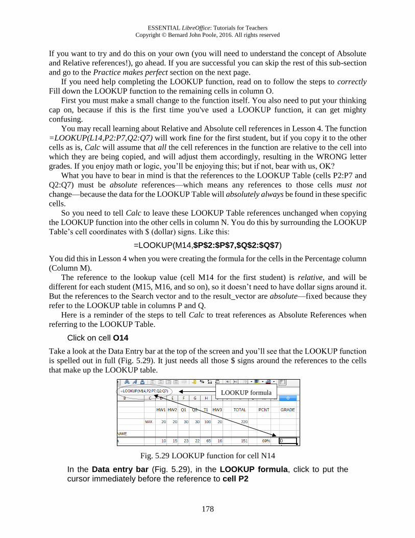
Take a look at the Data Entry bar at the top of the screen and you’ll see that the LOOKUP function
is spelled out in full (Fig. 5.29). It just needs all those $ signs around the references to the cells
that make up the LOOKUP table.
Fig. 5.29 LOOKUP function for cell N14
In the Data entry bar (Fig. 5.29), in the LOOKUP formula, click to put the cursor immediately before the reference to cell P2
LOOKUP formula
Lesson 5: More on the Use of the Spreadsheet
179
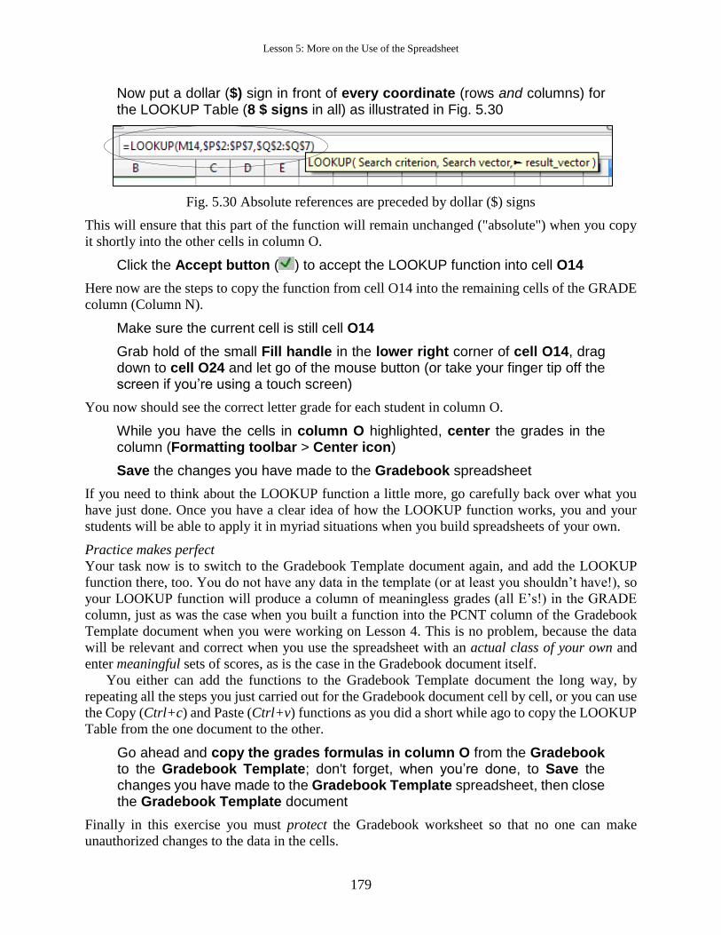
Now put a dollar ($) sign in front of every coordinate (rows and columns) for the LOOKUP Table (8 $ signs in all) as illustrated in Fig. 5.30
Fig. 5.30 Absolute references are preceded by dollar ($) signs
This will ensure that this part of the function will remain unchanged ("absolute") when you copy
it shortly into the other cells in column O.
Click the Accept button ( ) to accept the LOOKUP function into cell O14
Here now are the steps to copy the function from cell O14 into the remaining cells of the GRADE
column (Column N).
Make sure the current cell is still cell O14
Grab hold of the small Fill handle in the lower right corner of cell O14, drag down to cell O24 and let go of the mouse button (or take your finger tip off the screen if you’re using a touch screen)
You now should see the correct letter grade for each student in column O.
While you have the cells in column O highlighted, center the grades in the column (Formatting toolbar > Center icon)
Save the changes you have made to the Gradebook spreadsheet
If you need to think about the LOOKUP function a little more, go carefully back over what you
have just done. Once you have a clear idea of how the LOOKUP function works, you and your
students will be able to apply it in myriad situations when you build spreadsheets of your own.
Practice makes perfect
Your task now is to switch to the Gradebook Template document again, and add the LOOKUP
function there, too. You do not have any data in the template (or at least you shouldn’t have!), so
your LOOKUP function will produce a column of meaningless grades (all E’s!) in the GRADE
column, just as was the case when you built a function into the PCNT column of the Gradebook
Template document when you were working on Lesson 4. This is no problem, because the data
will be relevant and correct when you use the spreadsheet with an actual class of your own and
enter meaningful sets of scores, as is the case in the Gradebook document itself.
You either can add the functions to the Gradebook Template document the long way, by
repeating all the steps you just carried out for the Gradebook document cell by cell, or you can use
the Copy (Ctrl+c) and Paste (Ctrl+v) functions as you did a short while ago to copy the LOOKUP
Table from the one document to the other.
Go ahead and copy the grades formulas in column O from the Gradebook to the Gradebook Template; don't forget, when you’re done, to Save the changes you have made to the Gradebook Template spreadsheet, then close the Gradebook Template document
Finally in this exercise you must protect the Gradebook worksheet so that no one can make
unauthorized changes to the data in the cells.
ESSENTIAL LibreOffice: Tutorials for Teachers
Copyright © Bernard John Poole, 2016. All rights reserved
180
Select all the cells in the Gradebook worksheet (Ctrl+a), then, in the Tools menu > Protect Sheet… and in the Protect Sheet dialog box click to remove the check mark/tick in front of Select Unprotected Cells
Do the same for the Gradebook Template worksheet
Save your work and close just the Gradebook Template document
You should now have only the Gradebook document open on your screen.
5.6 PRINTING THE UPDATED SPREADSHEET If you are able to do so, you're going to print out the Gradebook document twice. Here are the
steps for the first printout.
It is usually best to print a spreadsheet in landscape (sideways) orientation.
In the Format menu > Page… dialog box, click on the Page tab and, in the Orientation section, click on the radio button next to Landscape Orientation
You need to take care of a couple of other details before clicking on the Print button. The printed
spreadsheet will look better if you remove column and row headings as well as the cell Grid Lines.
In the View menu click on Column & Row Headers to remove the check mark there, thus removing column and row headers from the spreadsheet
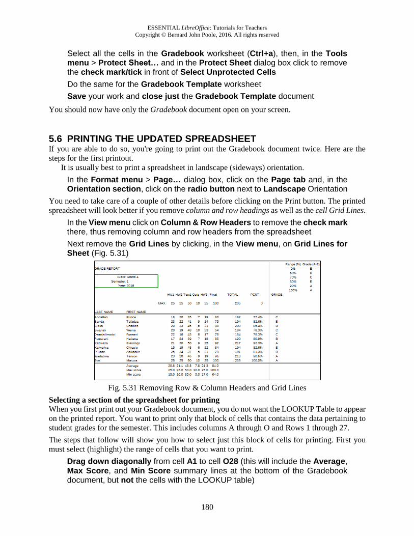
Next remove the Grid Lines by clicking, in the View menu, on Grid Lines for Sheet (Fig. 5.31)
Fig. 5.31 Removing Row & Column Headers and Grid Lines
Selecting a section of the spreadsheet for printing
When you first print out your Gradebook document, you do not want the LOOKUP Table to appear
on the printed report. You want to print only that block of cells that contains the data pertaining to
student grades for the semester. This includes columns A through O and Rows 1 through 27.
The steps that follow will show you how to select just this block of cells for printing. First you
must select (highlight) the range of cells that you want to print.
Drag down diagonally from cell A1 to cell O28 (this will include the Average, Max Score, and Min Score summary lines at the bottom of the Gradebook document, but not the cells with the LOOKUP table)
Lesson 5: More on the Use of the Spreadsheet
181
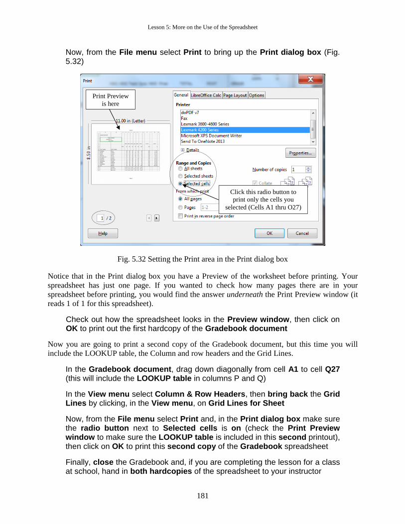
Now, from the File menu select Print to bring up the Print dialog box (Fig. 5.32)
Fig. 5.32 Setting the Print area in the Print dialog box
Notice that in the Print dialog box you have a Preview of the worksheet before printing. Your
spreadsheet has just one page. If you wanted to check how many pages there are in your
spreadsheet before printing, you would find the answer underneath the Print Preview window (it
reads 1 of 1 for this spreadsheet).
Check out how the spreadsheet looks in the Preview window, then click on OK to print out the first hardcopy of the Gradebook document
Now you are going to print a second copy of the Gradebook document, but this time you will
include the LOOKUP table, the Column and row headers and the Grid Lines.
In the Gradebook document, drag down diagonally from cell A1 to cell Q27 (this will include the LOOKUP table in columns P and Q)
In the View menu select Column & Row Headers, then bring back the Grid Lines by clicking, in the View menu, on Grid Lines for Sheet
Now, from the File menu select Print and, in the Print dialog box make sure the radio button next to Selected cells is on (check the Print Preview window to make sure the LOOKUP table is included in this second printout), then click on OK to print this second copy of the Gradebook spreadsheet
Finally, close the Gradebook and, if you are completing the lesson for a class at school, hand in both hardcopies of the spreadsheet to your instructor
Click this radio button to
print only the cells you
selected (Cells A1 thru O27)
Print Preview
is here
ESSENTIAL LibreOffice: Tutorials for Teachers
Copyright © Bernard John Poole, 2016. All rights reserved
182
5.7 CREATING CHARTS BASED ON SPREADSHEET DATA The Calc charting capability
Today we are in danger of being overwhelmed by too much data, the raw material of information.
We even have an acronym for it—TMI—too much information. It is a genuine problem.
One of many solutions to TMI is charts—graphic, colorful, eye-catching. Charts—quality
charts that don’t mess with the data—try to reduce the masses of data on any particular subject to
a meaningful analysis of what’s going on. This applies as much to the meaning of world events as
it does to the progress of an individual student in your class. Charts, in other words, are a powerful
way to convey what would otherwise be complex information.
Calc makes it easy to create dozens of different types of charts. You can create a chart from
information gathered in most any spreadsheet. It is not an exaggeration to say that your ability to
use Calc’s charting capability will make you a more effective teacher.
A spreadsheet user can take advantage of charts based on the numbers stored in its rows and
columns of cells. The numbers on their own may not provide much information. Charts based on
those numbers, on the oth35er hand, may enable the user to visualize the data. "A picture," as they
say, "is worth a thousand words."
A well-designed chart can help you (and your students) make sense of a thousand numbers.
Charts are also useful when you need to increase the impact of any oral or written presentation.
Think of the many charts that you now see presented on TV and in other media; their purpose is
to help you make sense of all the data out there, whether it’s business data, weather data, data
related to politics, and so on.
We must be wary of charts, of course, because, like statistics, they can be guilty of purveying,
well, lies. But charts that are well-designed and honestly-designed will help your students
understand what they need to know. More to the point, if you teach your students how to create
charts, they will be able to include them in assignments related to every subject area under the sun.
Creating a Column chart
For this exercise, we’ll set aside the work we’ve been doing with the Gradebook documents. You
are going to open a new spreadsheet document with data related to Grades so that you can practice
creating charts.
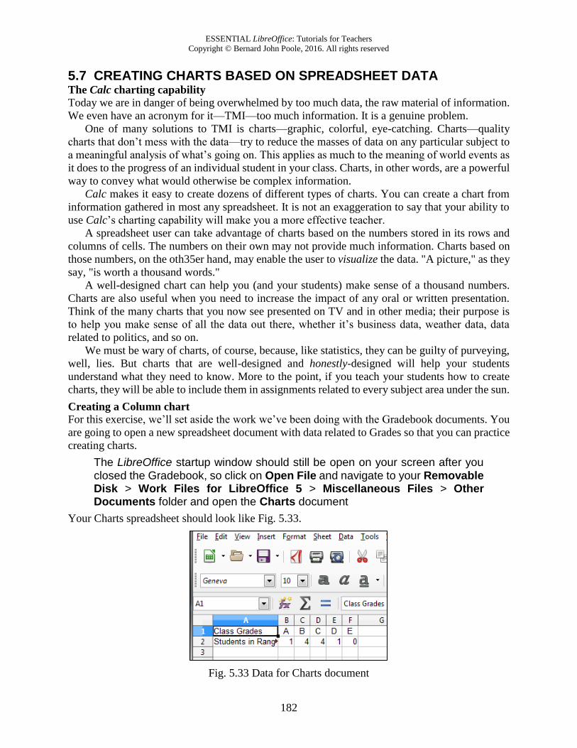
The LibreOffice startup window should still be open on your screen after you closed the Gradebook, so click on Open File and navigate to your Removable Disk > Work Files for LibreOffice 5 > Miscellaneous Files > Other Documents folder and open the Charts document
Your Charts spreadsheet should look like Fig. 5.33.
Fig. 5.33 Data for Charts document
Lesson 5: More on the Use of the Spreadsheet
183
The values represented in a chart are called a data series or data set. In the chart you are about to
create, the number of students in the various grade ranges (A, B, C, etc.) will be represented by
bars. The chart will have a title and a legend with names descriptive of the data series.
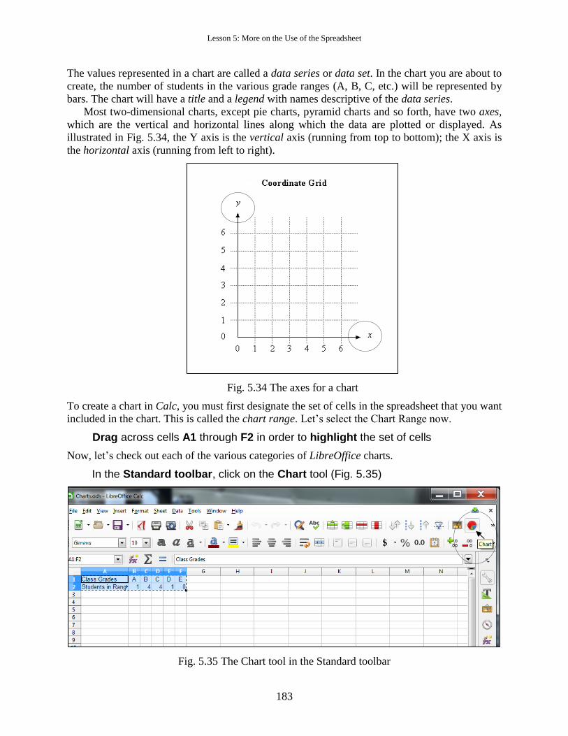
Most two-dimensional charts, except pie charts, pyramid charts and so forth, have two axes,
which are the vertical and horizontal lines along which the data are plotted or displayed. As
illustrated in Fig. 5.34, the Y axis is the vertical axis (running from top to bottom); the X axis is
the horizontal axis (running from left to right).
Fig. 5.34 The axes for a chart
To create a chart in Calc, you must first designate the set of cells in the spreadsheet that you want
included in the chart. This is called the chart range. Let’s select the Chart Range now.
Drag across cells A1 through F2 in order to highlight the set of cells
Now, let’s check out each of the various categories of LibreOffice charts.
In the Standard toolbar, click on the Chart tool (Fig. 5.35)
Fig. 5.35 The Chart tool in the Standard toolbar
ESSENTIAL LibreOffice: Tutorials for Teachers
Copyright © Bernard John Poole, 2016. All rights reserved
184
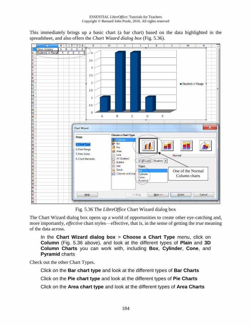
This immediately brings up a basic chart (a bar chart) based on the data highlighted in the
spreadsheet, and also offers the Chart Wizard dialog box (Fig. 5.36).
Fig. 5.36 The LibreOffice Chart Wizard dialog box
The Chart Wizard dialog box opens up a world of opportunities to create other eye-catching and,
more importantly, effective chart styles—effective, that is, in the sense of getting the true meaning
of the data across.
In the Chart Wizard dialog box > Choose a Chart Type menu, click on Column (Fig. 5.36 above), and look at the different types of Plain and 3D Column Charts you can work with, including Box, Cylinder, Cone, and Pyramid charts
Check out the other Chart Types.
Click on the Bar chart type and look at the different types of Bar Charts
Click on the Pie chart type and look at the different types of Pie Charts
Click on the Area chart type and look at the different types of Area Charts
One of the Normal
Column charts
Lesson 5: More on the Use of the Spreadsheet
185
Click on the Line chart type and look at the different types of Line Charts
Click on the XY (Scatter) chart type and look at the different types of Scatter Charts
Click on the Bubble chart type and look at the different types of Bubble Charts
Click on the Net chart type and look at the different types of Net Charts
Click on the Stock chart type and look at the different types of Stock Charts
Finally, click on the Column and Line chart type and look at the different types of Column and Line Charts
Quite a selection—dozens of different kinds of charts. But let’s focus for now on the Column
charts.
Click on the Column charts type
In the Column Charts options, click to put a check mark in the box next to 3D Look (Fig. 5.36 on previous page) then, in the Shape menu, click on Box (Fig. 5.36 again), and then click on the first Normal type of Column chart (Fig. 5.36)
As you see, Calc immediately creates the chart and displays it on the screen (Fig. 5.36 previous
page).
Notice that Calc has automatically put the grades along the (horizontal) X axis and the scale
indicating the number of students “in Range”—i.e. the number of students with each grade—along
the (vertical) Y axis.
One change you need to make right now is to the chart title. It should say something like “Class
Grades.” While we’re doing that we can make a couple of other changes as well.
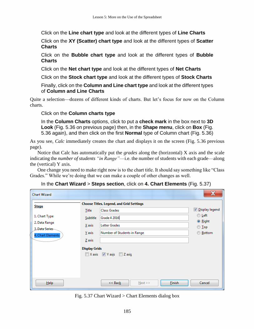
In the Chart Wizard > Steps section, click on 4. Chart Elements (Fig. 5.37)
Fig. 5.37 Chart Wizard > Chart Elements dialog box
ESSENTIAL LibreOffice: Tutorials for Teachers
Copyright © Bernard John Poole, 2016. All rights reserved
186
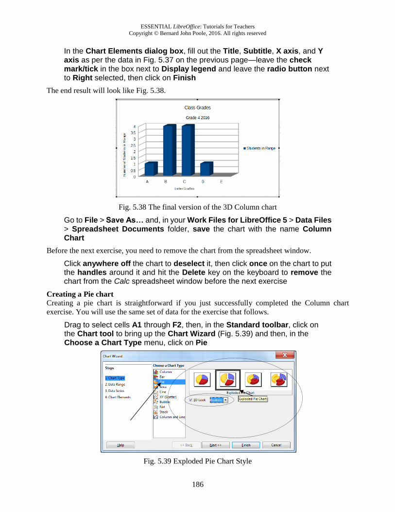
In the Chart Elements dialog box, fill out the Title, Subtitle, X axis, and Y axis as per the data in Fig. 5.37 on the previous page—leave the check mark/tick in the box next to Display legend and leave the radio button next to Right selected, then click on Finish
The end result will look like Fig. 5.38.
Fig. 5.38 The final version of the 3D Column chart
Go to File > Save As… and, in your Work Files for LibreOffice 5 > Data Files > Spreadsheet Documents folder, save the chart with the name Column Chart
Before the next exercise, you need to remove the chart from the spreadsheet window.
Click anywhere off the chart to deselect it, then click once on the chart to put the handles around it and hit the Delete key on the keyboard to remove the chart from the Calc spreadsheet window before the next exercise
Creating a Pie chart
Creating a pie chart is straightforward if you just successfully completed the Column chart
exercise. You will use the same set of data for the exercise that follows.
Drag to select cells A1 through F2, then, in the Standard toolbar, click on the Chart tool to bring up the Chart Wizard (Fig. 5.39) and then, in the Choose a Chart Type menu, click on Pie
Fig. 5.39 Exploded Pie Chart Style
Lesson 5: More on the Use of the Spreadsheet
187
In the Pie Charts dialog, click to put a check mark next to 3D Look and, in the 3D Look menu make sure the Realistic option is selected
In the Chart Wizard, click on each of the four Pie Chart styles and check them out before proceeding with the exercise
The style of Pie Chart you are going to work with is the Exploded Pie Chart (Fig. 5.39 above).
In the Steps section on the left of the Chart Wizard dialog box, click on 4. Chart Elements and change the Title to Class Grades Distribution as you did for the Column Chart, type Grade 4 2016 for the Subtitle
Leave the check mark/tick in the box next to Display legend and leave the radio button next to Right selected, then click on Finish
Now, right click on any of the slices in the Pie chart and, in the context menu that pops up, select the option to Insert Data Labels
This puts a label on each of the slices indicating how many students got that particular grade, thus
adding information to the chart. It would be helpful if the Font size were bigger on each of those
slices and maybe the color white would stand out more against the colors of the various slices.
This is easy enough to do.
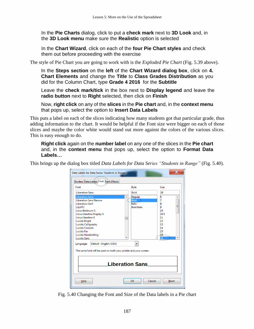
Right click again on the number label on any one of the slices in the Pie chart and, in the context menu that pops up, select the option to Format Data Labels…
This brings up the dialog box titled Data Labels for Data Series “Students in Range” (Fig. 5.40).
Fig. 5.40 Changing the Font and Size of the Data labels in a Pie chart
ESSENTIAL LibreOffice: Tutorials for Teachers
Copyright © Bernard John Poole, 2016. All rights reserved
188
Click on the Font tab and change the Style to Bold and the font size to 18
Next click on the Font Effects tab and change the Font Color to White
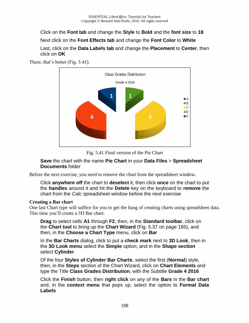
Last, click on the Data Labels tab and change the Placement to Center, then click on OK
There, that’s better (Fig. 5.41).
Fig. 5.41 Final version of the Pie Chart
Save the chart with the name Pie Chart in your Data Files > Spreadsheet Documents folder
Before the next exercise, you need to remove the chart from the spreadsheet window.
Click anywhere off the chart to deselect it, then click once on the chart to put the handles around it and hit the Delete key on the keyboard to remove the chart from the Calc spreadsheet window before the next exercise
Creating a Bar chart
One last Chart type will suffice for you to get the hang of creating charts using spreadsheet data.
This time you’ll create a 3D Bar chart.
Drag to select cells A1 through F2, then, in the Standard toolbar, click on the Chart tool to bring up the Chart Wizard (Fig. 5.37 on page 185), and then, in the Choose a Chart Type menu, click on Bar
In the Bar Charts dialog, click to put a check mark next to 3D Look, then in the 3D Look menu select the Simple option, and in the Shape section select Cylinder
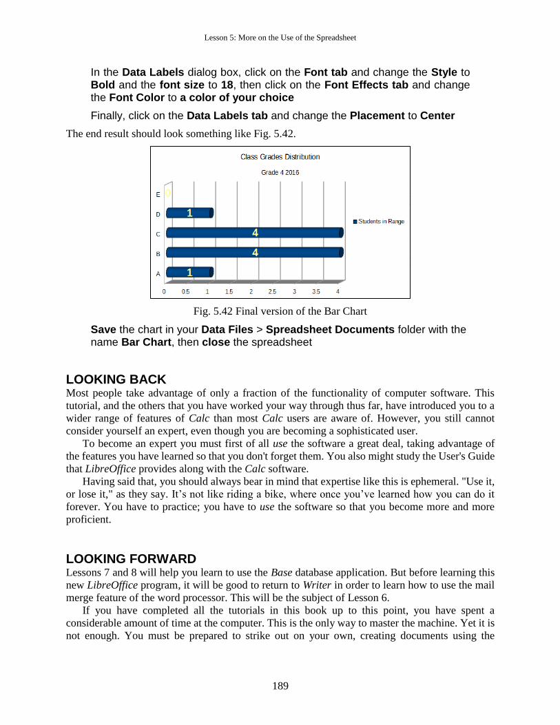
Of the four Styles of Cylinder Bar Charts, select the first (Normal) style, then, in the Steps section of the Chart Wizard, click on Chart Elements and type the Title Class Grades Distribution, with the Subtitle Grade 4 2016
Click the Finish button, then right click on any of the Bars in the Bar chart and, in the context menu that pops up, select the option to Format Data Labels
Lesson 5: More on the Use of the Spreadsheet
189
In the Data Labels dialog box, click on the Font tab and change the Style to Bold and the font size to 18, then click on the Font Effects tab and change the Font Color to a color of your choice
Finally, click on the Data Labels tab and change the Placement to Center
The end result should look something like Fig. 5.42.
Fig. 5.42 Final version of the Bar Chart
Save the chart in your Data Files > Spreadsheet Documents folder with the name Bar Chart, then close the spreadsheet
LOOKING BACK Most people take advantage of only a fraction of the functionality of computer software. This
tutorial, and the others that you have worked your way through thus far, have introduced you to a
wider range of features of Calc than most Calc users are aware of. However, you still cannot
consider yourself an expert, even though you are becoming a sophisticated user.
To become an expert you must first of all use the software a great deal, taking advantage of
the features you have learned so that you don't forget them. You also might study the User's Guide
that LibreOffice provides along with the Calc software.
Having said that, you should always bear in mind that expertise like this is ephemeral. "Use it,
or lose it," as they say. It’s not like riding a bike, where once you’ve learned how you can do it
forever. You have to practice; you have to use the software so that you become more and more
proficient.
LOOKING FORWARD Lessons 7 and 8 will help you learn to use the Base database application. But before learning this
new LibreOffice program, it will be good to return to Writer in order to learn how to use the mail
merge feature of the word processor. This will be the subject of Lesson 6.
If you have completed all the tutorials in this book up to this point, you have spent a
considerable amount of time at the computer. This is the only way to master the machine. Yet it is
not enough. You must be prepared to strike out on your own, creating documents using the
ESSENTIAL LibreOffice: Tutorials for Teachers
Copyright © Bernard John Poole, 2016. All rights reserved
190
productivity tools you are learning in these tutorials to meet your needs both in and out of the
classroom.
Deep, assimilated learning takes place only once you are working independently, because to
do this you have to show that you have understood everything you have learned. Understanding
leads to transference and acquisition of skills. Tutorials will open the doors to knowledge, and hold
your hand while you make those first steps toward the acquisition of specific skills.
But you must have the desire to let go of the hand that guides you. Without this desire, the
exercises that you are following will be wasted and yield no fruit. With this desire, you will be
motivated to understand what you are learning so that you can apply it to new situations in your
own professional experience.
SKILL CONSOLIDATION Complete these exercises to reinforce what you have learned in Lesson 5.
1. List at least 5 applications, other than those presented in these tutorials, for which you think
you would use the Calc spreadsheet in a classroom environment.
2. Either alone, or with a group, develop templates for each of the five spreadsheets identified in
exercise 1. This could be an excellent class project. Each team would develop a different set
of templates. Then all groups would present their results for review by everyone else in the
class, and the complete set of templates could be made available on disk for everyone to take
away from the course.
3. Load the Gradebook document to the Desktop.
• Add the function to calculate the average score for each of the tests, quizzes, homework,
etc. The system will add up all the scores and divide by the number of cells that contain
scores to arrive at the average. You should use the copy function to duplicate the
functions across the spreadsheet.
• Save the updated document
• Print out only the columns that contain the student names and the final totals and
percentages (so you will need to temporarily delete the columns in between—don't save
this document!)
4. Load the Gradebook document onto the Desktop.
• Add a new column for another set of scores
• Add a new row for another student
• Update the functions where necessary
• Sort the student records based on the First and Last Name columns
• Save the updated document
5. Create a line chart based on a set of values for populations in several cities in Malawi. Generate
a Column chart, Bar chart, and Pie chart from the data. Research the population data on the
web at http://countrymeters.info/en/Malawi
6. Create a Column chart, Bar chart, and Pie chart based on a set of values for the amount of
rainfall for each of a selection of cities in Malawi. Research the Malawi rainfall data at this
web address: http://www.worldclimate.com/cgi-bin/grid.pl?gr=S13E033