Embed Size (px)
Citation preview

Chapter 15
Integral Transforms
15.1 Introduction and Definitions
Frequently in physics we encounter pairs of functions related by an integralof the form
F(α) =∫ b
a
f (t)K(α, t)dt. (15.1)
The function F(α) is called the (integral) transform of f (t) by the kernelK(α, t). The operation may also be described as mapping a function f (t) int-space into another function F(α) in α-space. This interpretation takes onphysical significance in the time–frequency relation of Fourier transforms,such as Example 15.4.4.
Linearity
These integral transforms are linear operators; that is,∫ b
a
[c1 f1(t) + c2 f2(t)]K(α, t)dt
= c1
∫ b
a
f1(t)K(α, t)dt + c2
∫ b
a
f2(t)K(α, t)dt, (15.2)
= c1 F1(α) + c2 F2(α),∫ b
a
c f (t)K(α, t)dt = c
∫ b
a
f (t)K(α, t)dt, (15.3)
where c1, c2, c are constants, and f1(t), f2(t) are functions for which the inte-gral transform is well defined.
689
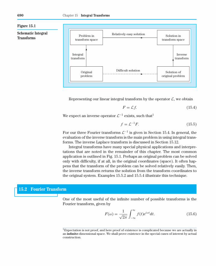
690 Chapter 15 Integral Transforms
Problem intransform space
Originalproblem
Integraltransform
Relatively easy solution
Difficult solution
Solution intransform space
Solution oforiginal problem
Inversetransform
Figure 15.1
Schematic IntegralTransforms
Representing our linear integral transform by the operator L, we obtain
F = L f. (15.4)
We expect an inverse operator L−1 exists, such that1
f = L−1 F. (15.5)
For our three Fourier transforms L−1 is given in Section 15.4. In general, theevaluation of the inverse transform is the main problem in using integral trans-forms. The inverse Laplace transform is discussed in Section 15.12.
Integral transforms have many special physical applications and interpre-tations that are noted in the remainder of this chapter. The most commonapplication is outlined in Fig. 15.1. Perhaps an original problem can be solvedonly with difficulty, if at all, in the original coordinates (space). It often hap-pens that the transform of the problem can be solved relatively easily. Then,the inverse transform returns the solution from the transform coordinates tothe original system. Examples 15.5.2 and 15.5.4 illustrate this technique.
15.2 Fourier Transform
One of the most useful of the infinite number of possible transforms is theFourier transform, given by
F(ω) = 1√2π
∫ ∞
−∞f (t)eiωtdt. (15.6)
1Expectation is not proof, and here proof of existence is complicated because we are actually inan infinite-dimensional space. We shall prove existence in the special cases of interest by actualconstruction.

15.2 Fourier Transform 691
Two modifications of this form, developed in Section 15.4, are the Fouriercosine and Fourier sine transforms:
Fc(ω) =√
2π
∫ ∞
0f (t) cos ωt dt, (15.7)
Fs(ω) =√
2π
∫ ∞
0f (t) sin ωt dt. (15.8)
All these integrals exist if∫ ∞−∞ | f (t)|dt < ∞, a condition denoted f ∈
L(−∞, ∞) in the mathematical literature and meaning that the function f
belongs to the space of absolutely integrable functions. Moreover, thenRiemann’s lemma holds
∫ ∞
−∞f (t) cos ωt dt → 0,
∫ ∞
−∞f (t) sin ωt dt → 0, as ω → ∞.
The Fourier transform is based on the kernel eiωt and its real and imaginaryparts taken separately, cos ωt and sin ωt. Because these kernels are the func-tions used to describe waves, due to their periodicity, Fourier transformsappear frequently in studies of waves and the extraction of information fromwaves, particularly when phase information is involved. The output of a stel-lar interferometer, for instance, involves a Fourier transform of the bright-ness across a stellar disk. The electron charge distribution in an atom maybe obtained from a Fourier transform of the amplitude of scattered X-rays.In quantum mechanics the physical origin of the Fourier relations of Section15.7 is the wave nature of matter and our description of matter in terms ofwaves.
If we differentiate the Fourier transform
dF(ω)dω
= i√2π
∫ ∞
−∞t f (t)eiωtdt,
we see that the original function f (t) is multiplied by it. This is one way ofgenerating new Fourier transforms.
If we differentiate a cosine transform with respect to ω, we are led to asine transform and vice versa. Many examples are given by Titchmarsh (seeAdditional Reading).
EXAMPLE 15.2.1 Square Pulse Let us find the Fourier transform for the shape in Fig. 15.2:
f (t) ={
1, |t| < 1,
0, |t| > 1,
which is an even function of t. This is the single slit diffraction problem ofphysical optics. The slit is described by f (t). The diffraction pattern amplitude
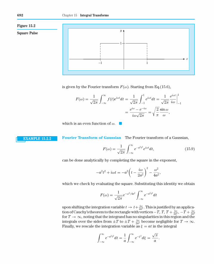
692 Chapter 15 Integral Transforms
−1
1
1x
y
Figure 15.2
Square Pulse
is given by the Fourier transform F(ω). Starting from Eq.(15.6),
F(ω) = 1√2π
∫ ∞
−∞f (t)eiωtdt = 1√
2π
∫ 1
−1eiωtdt = 1√
2π
eiωt
iω
∣∣∣∣1
−1
= eiω − e−iω
iω√
2π=
√2π
sin ω
ω,
which is an even function of ω. ■
EXAMPLE 15.2.2 Fourier Transform of Gaussian The Fourier transform of a Gaussian,
F(ω) = 1√2π
∫ ∞
−∞e−a2t2
eiωtdt, (15.9)
can be done analytically by completing the square in the exponent,
−a2t2 + iωt = −a2(
t − iω
2a2
)2
− ω2
4a2,
which we check by evaluating the square. Substituting this identity we obtain
F(ω) = 1√2π
e−ω2/4a2∫ ∞
−∞e−a2t2
dt
upon shifting the integration variable t → t+ iω2a2 . This is justified by an applica-
tion of Cauchy’s theorem to the rectangle with vertices−T, T, T + iω2a2 , −T + iω
2a2
for T → ∞, noting that the integrand has no singularities in this region and theintegrals over the sides from ±T to ±T + iω
2a2 become negligible for T → ∞.
Finally, we rescale the integration variable as ξ = at in the integral
∫ ∞
−∞e−a2t2
dt = 1a
∫ ∞
−∞e−ξ 2
dξ =√
π
a.
15.2 Fourier Transform 693
Substituting these results we find
F(ω) = 1
a√
2exp
(− ω2
4a2
), (15.10)
again a Gaussian, but in ω-space. The smaller a is (i.e., the wider the originalGaussian e−a2t2
is), the narrower is its Fourier transform ∼e−ω2/4a2. Differenti-
ating F(ω), the Fourier transform of iωe−ω2/4a2is ∼te−a2t2
, etc. ■
Laplace Transform
The equally important Laplace transform is related to a Fourier transformby replacing the frequency ω with an imaginary variable and changing theintegration interval, that is, exp(iωx) → exp(−sx), which will be developedin Sections 15.8–15.12. The Laplace transform
F(s) =∫ ∞
0f (t)e−stdt (15.11)
has the kernel e−st. Clearly, the possible types of integral transforms are unlim-ited. The Laplace transform has been useful in mathematical analysis as well asin physics and engineering applications. The Laplace and Fourier transformsare by far the most used. For Mellin, Hankel, Bessel, and other transforms, seeAdditional Reading.
If the integrand of a Fourier integral is analytic, then the integral may beevaluated using the residue theorem according to Eq. (7.30). See Example 7.2.3and Exercises 7.2.4 and 7.2.15. The same method applies to Laplace transforms.
EXAMPLE 15.2.3 Euler Integral as Laplace Transform If we generalize the Euler integral[Eq. (10.5)] to∫ ∞
0e−sttz dt = 1
sz+1
∫ ∞
0e−st(st)z d(st) = (z + 1)
sz+1,
where z is a complex parameter with �(z) > −1, the Laplace transform of thepower tz is the inverse power s−z−1 up to the normalization factor (z+1). ■
Laplace transforms will be treated in detail starting in Section 15.8.
EXERCISES
15.2.1 (a) Show that F(−ω) = F∗(ω) is a necessary and sufficient conditionfor the Fourier transform f (t) to be real.
(b) Show that F(−ω) = −F∗(ω) is a necessary and sufficient conditionfor f (t) to be pure imaginary.
15.2.2 Let F(ω) be the Fourier (exponential) transform of f (t) and G(ω) theFourier transform of g(t) = f (t + a). Show that
G(ω) = e−iaω F(ω).
15.2.3 Prove the identities involved in Exercise 6.5.15.
694 Chapter 15 Integral Transforms
15.2.4 Find the Fourier sine and cosine transforms of e−a|t|.
15.2.5 Find the Fourier exponential, sine, and cosine transforms of e−a|t| cos bt
and e−a|t| sin bt.
15.2.6 Find the Fourier exponential, sine, and cosine transforms of 1/(a2+t2)n
for n = 2, 3.
15.3 Development of the Inverse Fourier Transform
Fourier series, such as∑
n an cos(nπ t/L), that we studied in the previouschapter are sums of terms each involving a multiple n�ω of a basic frequencyω = nπ/L. If we let the periodicity interval of length L → ∞, then n�ω be-comes a continuous frequency variable ω, and the Fourier series goes over intoa Fourier integral A(t) = ∫ ∞
−∞ a(ω) cos ωt dω for a nonperiodic function A(t).This transition from Fourier series to integral is now described in more detail.
In Chapter 14, it was shown that Fourier series are useful in representingcertain functions over a limited range [0, 2π ], [−L, L], and so on, if the func-tion is periodic. We now turn our attention to the problem of representinga nonperiodic function over the infinite range, letting L → ∞. Physically,this sometimes means resolving a single pulse or wave packet into sinusoidalwaves or a temperature distribution that decays at ±∞ into wave components.
We have seen (Section 14.2) that for the interval [−L, L] the coefficientsan and bn could be written as
an = 1L
∫ L
−L
f (t) cosnπ t
Ldt, (15.12)
bn = 1L
∫ L
−L
f (t) sinnπ t
Ldt. (15.13)
The resulting Fourier series
f (x) = 12L
∫ L
−L
f (t)dt + 1L
∞∑n=1
cosnπx
L
∫ L
−L
f (t) cosnπ t
Ldt
+ 1L
∞∑n=1
sinnπx
L
∫ L
−L
f (t) sinnπ t
Ldt (15.14)
or
f (x) = 12L
∫ L
−L
f (t)dt + 1L
∞∑n=1
∫ L
−L
f (t) cosnπ
L(t − x)dt (15.15)
is Eq. (14.28). However, we now let the parameter L approach infinity, trans-forming the finite interval [−L, L] into the infinite interval (−∞, ∞). We set
nπ
L= ω,
π
L= �ω, with L → ∞.

15.3 Development of the Inverse Fourier Transform 695
Then we have
f (x) → 1π
∞∑n=1
�ω
∫ ∞
−∞f (t) cos ω(t − x)dt (15.16)
or
f (x) = 1π
∫ ∞
0dω
∫ ∞
−∞f (t) cos ω(t − x)dt, (15.17)
replacing the infinite sum by the integral over ω. The first term (correspond-ing to a0) has been absorbed at ω = 0, assuming that
∫ ∞−∞ f (t)dt exists. This
Fourier cosine formula is valid if f is continuous at x. If f is only piecewisecontinuous, then f (x) must be replaced by 1
2 [ f (x+0)+ f (x−0)], which is theaverage of the limiting values of f to the left and right of the point x. Also, inte-grals
∫ ∞−∞ f (t)dt, etc., are always understood as the limit limT→∞
∫ T
−Tf (t)dt.
It must be emphasized that this Fourier integral representation of f (x) [Eq.(15.17)] is purely formal. It is not intended as a rigorous derivation, but it canbe made rigorous (compare I. N. Sneddon, Fourier Transforms, Section 3.2;see Additional Reading). It is subject to the conditions that f (x) is
• piecewise continuous;• differentiable almost everywhere (of bounded variation); and• absolutely integrable; that is,
∫ ∞−∞ | f (x)|dx is finite.
Inverse Fourier Transform---Exponential Form
Our Fourier integral [Eq. (15.17)] may be put into exponential form by notingthat because cos ω(t − x) is an even function of ω and sin ω(t − x) is an oddfunction of ω,
f (x) = 12π
∫ ∞
−∞dω
∫ ∞
−∞f (t) cos ω(t − x)dt, (15.18)
whereas1
2π
∫ ∞
−∞dω
∫ ∞
−∞f (t) sin ω(t − x)dt = 0. (15.19)
Adding Eqs. (15.18) and (15.19) (with a factor i), we obtain
f (x) = 1√2π
∫ ∞
−∞e−iωxdω
1√2π
∫ ∞
−∞f (t)eiωtdt (15.20)
or, in terms of the Fourier transform F(ω) of f (t),
f (x) = 1√2π
∫ ∞
−∞F(ω)e−iωxdω, F(ω) = 1√
2π
∫ ∞
−∞f (t)eiωtdt. (15.21)
The variable ω introduced here is an arbitrary mathematical variable. In manyphysical problems, however, t and x are time variables and then ω correspondsto a frequency. We may then interpret Eq. (15.18) or Eq. (15.20) as a represen-tation of f (x) in terms of a distribution of infinitely long sinusoidal wave trainsof angular frequency ω in which this frequency is a continuous variable.

696 Chapter 15 Integral Transforms
EXAMPLE 15.3.1 Inversion of Square Pulse Using the Fourier transform in Example 15.2.1,the square pulse can now be inverted as follows:
f (t) = 1√2π
∫ ∞
−∞
√2π
sin ω
ωe−iωtdω = 1
π
∫ ∞
−∞
sin ω
ωe−iωtdω.
Splitting the integral into one over (−∞, 0) and another over (0, ∞) gives
f (t) = 1π
∫ ∞
0
sin ω
ω(e−iωt + eiωt)dω = 2
π
∫ ∞
0
sin ω
ωcos ωt dω,
an inverse cosine transform.Alternatively, we can differentiate the Heaviside unit step function expres-
sion [using du(x)dx
= δ(x)]
f (t) = u(t + 1) − u(−1 + t) givingdf (t)
dt= δ(t + 1) − δ(−1 + t).
This yields
df (t)dt
= 12π
∫ ∞
−∞e−iωtdω
∫ ∞
−∞[δ(t′ + 1) − δ(t′ − 1)]e−iωt′
dt′
= 12π
∫ ∞
−∞e−iωt(eiω − e−iω)dω = i
π
∫ ∞
−∞e−iωt sin ω dω,
and by integrating the result f (t) = 1π
∫ ∞−∞ e−iωt sin ω
ωdω, as above. As a final
check, Exercise 7.2.15 gives us
f (t) = 1π
∫ ∞
−∞
sin ω
ωe−iωtdω =
{0, |t| > 1,
1, |t| < 1.■
Dirac Delta Function Derivation
If the order of integration of Eq. (15.20) is reversed, we may rewrite it as
f (x) =∫ ∞
−∞f (t)
{1
2π
∫ ∞
−∞eiω(t−x)dω
}dt. (15.22)
Apparently, the quantity in curly brackets behaves as a delta function δ(t − x).We might take Eq. (15.22) as presenting us with a Fourier integral represen-tation of the Dirac delta function. Alternatively, we take it as a clue to a newderivation of the Fourier integral theorem.
From Eq. (1.160) (shifting the singularity from t = 0 to t = x),
f (x) = limn→∞
∫ ∞
−∞f (t)δn(t − x)dt, (15.23)
where δn(t − x) is a sequence defining the distribution δ(t − x). Note thatEq. (15.23) assumes that f (t) is continuous at t = x. We take δn(t − x) to be
δn(t − x) = sin n(t − x)π(t − x)
= 12π
∫ n
−n
eiω(t−x)dω, (15.24)
15.3 Development of the Inverse Fourier Transform 697
using Eq. (1.156). Substituting Eq. (15.24) into Eq. (15.23), we have
f (x) = limn→∞
12π
∫ ∞
−∞f (t)
∫ n
−n
eiω(t−x)dω dt. (15.25)
Interchanging the order of integration and then taking the limit, as n → ∞, wehave Eq. (15.20), the Fourier integral theorem.
With the understanding that it belongs under an integral sign as in Eq.(15.22), the identification
δ(t − x) = 12π
∫ ∞
−∞eiω(t−x)dω (15.26)
provides a very useful Fourier integral representation of the delta func-
tion. It is used to great advantage in Sections 15.6 and 15.7.
EXERCISES
15.3.1 Prove that
h
2πi
∫ ∞
−∞
e−iωtdω
E0 − i/2 − hω=
{exp(−t/2h) exp(−iE0t/h), t > 0,
0, t < 0.
This Fourier integral appears in a variety of problems in quantum me-chanics: Wentzel, Kramers, Brillouin (WKB) barrier penetration, scat-tering, time-dependent perturbation theory, and so on.Hint. Try contour integration.
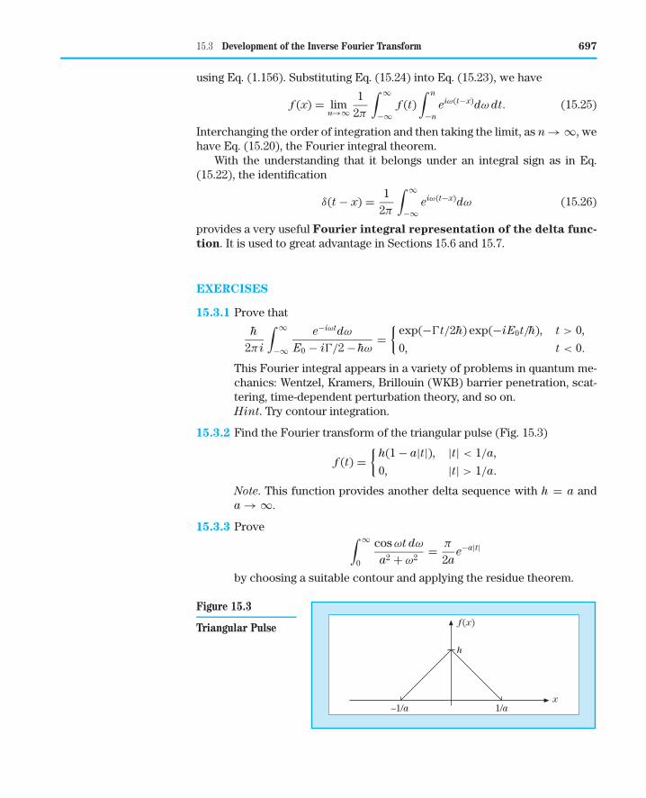
15.3.2 Find the Fourier transform of the triangular pulse (Fig. 15.3)
f (t) ={
h(1 − a|t|), |t| < 1/a,
0, |t| > 1/a.
Note. This function provides another delta sequence with h = a anda → ∞.
15.3.3 Prove ∫ ∞
0
cos ωt dω
a2 + ω2= π
2ae−a|t|
by choosing a suitable contour and applying the residue theorem.
h
x
f(x)
–1/a 1/a
Figure 15.3
Triangular Pulse
698 Chapter 15 Integral Transforms
15.3.4 Find the Fourier cosine, sine, and complex transforms of e−a2x2.
15.3.5 Define a sequence
δn(x) ={
n, |x| < 1/2n,
0, |x| > 1/2n.
[This is Eq.(1.153).] Express δn(x) as a Fourier integral and show thatwe may write
δ(x) = limn→∞ δn(x) = 1
2π
∫ ∞
−∞e−ikxdk.
15.3.6 Using the sequence
δn(x) = n√π
exp(−n2x2),
show that
δ(x) = 12π
∫ ∞
−∞e−ikxdk.
Note. Remember that δ(x) is defined in terms of its behavior as part ofan integrand [Section 1.14, especially Eqs. (1.151) and (1.152)].
15.4 Fourier Transforms---Inversion Theorem
Let us define F(ω), the Fourier transform of the function f (t), by
F(ω) ≡ 1√2π
∫ ∞
−∞f (t)eiωtdt. (15.27)
Exponential Transform
Then from Eq. (15.20) we have the inverse relation
f (t) = 1√2π
∫ ∞
−∞F(ω)e−iωtdω. (15.28)
Note that Eqs. (15.27) and (15.28) are almost but not quite symmetrical, differ-ing only in the sign of i.
Here two points deserve comment. First, the 1/√
2π symmetry is a matterof choice, not of necessity. Many authors attach the entire 1/(2π) factor ofEq. (15.20) to either Eq. (15.27) or Eq. (15.28). Second, although the Fourierintegral [Eq. (15.20)] has received much attention in the mathematics literature,we shall be primarily interested in the Fourier transform and its inverse. Theyare the equations with physical significance.
15.4 Fourier Transforms---Inversion Theorem 699
When we move the Fourier transform pair to three-dimensional space, itbecomes
F(k) = 1(2π)3/2
∫f (r)eik·rd3r, (15.29)
f (r) = 1(2π)3/2
∫F(k)e−ik·rd3k. (15.30)
The integrals are over all space. Verification, if desired, follows immediately bysubstituting the left-hand side of one equation into the integrand of the otherequation and using the three-dimensional delta function.2 Equation (15.30) maybe interpreted as an expansion of a function f (r) in a continuum of plane waveeigenfunctions; F(k) then becomes the amplitude of the wave exp(−ik · r).
Cosine Transform
If f (x) is odd or even, these transforms may be expressed in a different form.Consider, first, fc(x) = fc(−x), even. Writing the exponential of Eq. (15.27) intrigonometric form, we have
Fc(ω) = 1√2π
∫ ∞
−∞fc(t)(cos ωt + i sin ωt)dt
=√
2π
∫ ∞
0fc(t) cos ωt dt, (15.31)
the sin ωt dependence vanishing on integration over the symmetric interval(−∞, ∞). Similarly, since cos ωt is even, Eq. (15.27) transforms to
fc(t) =√
2π
∫ ∞
0Fc(ω) cos ωt dω. (15.32)
Equations (15.31) and (15.32) are known as Fourier cosine transforms.
EXAMPLE 15.4.1 Evaluation of Fourier Cosine Transform Evaluate the Fourier cosineintegral of e−ax with a a positive constant. Integrating by parts twice, we obtain
∫ ∞
0e−ax cos ωx dx = −1
ae−ax cos ωx
∣∣∣∣∞
0− ω
a
∫ ∞
0e−ax sin ωx dx
= 1a
− ω
a
[− 1
ae−ax sin ωx
∣∣∣∣∞
0+ ω
a
∫ ∞
0e−ax cos ωx dx
].
Now we combine the integral on the right-hand side with that on the left, giving(
1 + ω2
a2
) ∫ ∞
0e−ax cos ωx dx = 1
a
2δ(r1 − r2) = δ(x1 − x2)δ(y1 − y2)δ(z1 − z2) with Fourier integral δ(x1 − x2) =1
2π
∫ ∞−∞ exp[ik1(x1 − x2)]dk1, etc.
700 Chapter 15 Integral Transforms
or ∫ ∞
0e−ax cos ωx dx = a
a2 + ω2. ■
Sine Transform
The corresponding pair of Fourier sine transforms is obtained by assumingthat fs(x) = − fs(−x), odd, and applying the same symmetry arguments. Theequations are
Fs(ω) =√
2π
∫ ∞
0fs(t) sin ωt dt,3 (15.33)
fs(t) =√
2π
∫ ∞
0Fs(ω) sin ωt dω. (15.34)
From the last equation we may develop the physical interpretation that f (t)is being described by a continuum of sine waves. The amplitude of sin ωt isgiven by
√2/π Fs(ω), in which Fs(ω) is the Fourier sine transform of f (t). It will
be seen that Eq. (15.34) is the integral analog of the summation [Eq. (14.23)].Similar interpretations hold for the cosine and exponential cases.
EXAMPLE 15.4.2 Evaluation of Fourier Sine Transform Evaluate the Fourier sine integralof ω
a2+ω2 with a a positive constant. The denominator has the poles ω = ±ia,suggesting contour integration in the complex ω-plane. With this in mind, wereplace ω → −ω and show that
−∫ ∞
0
ωe−iωtdω
a2 + ω2=
∫ 0
−∞
ωeiωtdω
a2 + ω2
so that our Fourier sine integral becomes∫ ∞
0
ω sin ωt dω
a2 + ω2= 1
2i
∫ ∞
0
ω(eiωt − e−iωx)a2 + ω2
= 12i
∫ ∞
−∞
ωeiωt
a2 + ω2.
For t > 0, we close the contour in the upper ω-plane by a large half-circle,which does not contribute to the integral as its radius goes to ∞. We pick upthe residue iae−at/2ia at the pole ω = ia and find∫ ∞
0
ω sin ωt dω
a2 + ω2= π
2e−at. ■
If we take Eqs. (15.27), (15.31), and (15.33) as the direct integral trans-forms, described by L in Eq. (15.4) (Section 15.1), the corresponding inversetransforms, L−1 of Eq. (15.5), are given by Eqs. (15.28), (15.32), and (15.34).
3Note that a factor −i has been absorbed into this Fs(ω).
15.4 Fourier Transforms---Inversion Theorem 701
EXAMPLE 15.4.3 Proton Charge Form Factor The charge form factor
GE(q2) =∫
ρ(r)eiq·rd3r
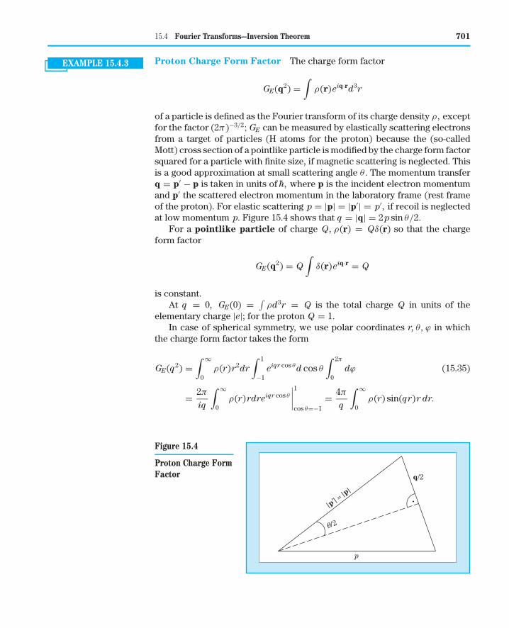
of a particle is defined as the Fourier transform of its charge density ρ , exceptfor the factor (2π)−3/2; GE can be measured by elastically scattering electronsfrom a target of particles (H atoms for the proton) because the (so-calledMott) cross section of a pointlike particle is modified by the charge form factorsquared for a particle with finite size, if magnetic scattering is neglected. Thisis a good approximation at small scattering angle θ. The momentum transferq = p′ − p is taken in units of h, where p is the incident electron momentumand p′ the scattered electron momentum in the laboratory frame (rest frameof the proton). For elastic scattering p = |p| = |p′| = p′, if recoil is neglectedat low momentum p. Figure 15.4 shows that q = |q| = 2p sin θ/2.
For a pointlike particle of charge Q, ρ(r) = Qδ(r) so that the chargeform factor
GE(q2) = Q
∫δ(r)eiq·r = Q
is constant.At q = 0, GE(0) = ∫
ρd3r = Q is the total charge Q in units of theelementary charge |e|; for the proton Q = 1.
In case of spherical symmetry, we use polar coordinates r, θ , ϕ in whichthe charge form factor takes the form
GE(q2) =∫ ∞
0ρ(r)r2dr
∫ 1
−1eiqr cos θd cos θ
∫ 2π
0dϕ (15.35)
= 2π
iq
∫ ∞
0ρ(r)rdreiqr cos θ
∣∣∣∣1
cos θ=−1= 4π
q
∫ ∞
0ρ(r) sin(qr)r dr.
p
|p′| = |p
|
q/2
q/2
Figure 15.4
Proton Charge FormFactor
702 Chapter 15 Integral Transforms
Inverting this sine transform, one can extract the charge density from themeasured charge form factor GE(q2). This is how the proton, nuclear radii,and sizes of atoms and molecules are measured by electron scattering.
At small q compared to the inverse radius of the proton, we can use thepower series for sin qr and obtain
GE(q2) = 4π
∫ ∞
0ρ(r)r2 dr − q2
6
∫ ∞
0ρ(r)r4 dr + · · · = 1 − q2
6〈r2〉 + · · · ,
where the first term is the charge Q = 1 and the integral in the second termis the mean square radius 〈r2〉 of the proton, because the density ρ = |ψ |2is given by the quark wave function ψ, quarks being the constituents of theproton. Thus, the proton size can be extracted from the measured slope of theproton charge form factor,
〈r2〉 = −6dGE(q2)
dq2
∣∣∣∣q=0
.
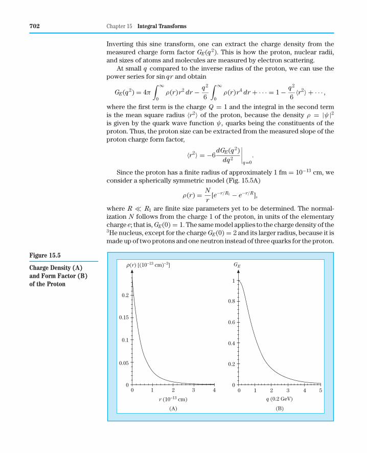
Since the proton has a finite radius of approximately 1 fm = 10−13 cm, weconsider a spherically symmetric model (Fig. 15.5A)
ρ(r) = N
r[e−r/R1 − e−r/R],
where R � R1 are finite size parameters yet to be determined. The normal-ization N follows from the charge 1 of the proton, in units of the elementarycharge e; that is, GE(0) = 1. The same model applies to the charge density of the3He nucleus, except for the charge GE(0) = 2 and its larger radius, because it ismade up of two protons and one neutron instead of three quarks for the proton.
0.05
00 1 2
r (10−13 cm)
3 4
(A) (B)
0.1
0.15
0.2
0.2
00 1 2
q (0.2 GeV)
3 4 5
0.4
0.6
0.8
1
GEr(r) [(10−13 cm)−3]
Figure 15.5
Charge Density (A)and Form Factor (B)of the Proton

15.4 Fourier Transforms---Inversion Theorem 703
Let us start by determining N from GE(0) = 1 by integrating by parts asfollows:
1 = 4π
∫ ∞
0ρ(r)r2 dr = 4π N
∫ ∞
0[e−r/R1 − e−r/R]r dr
= 4π N[−rR1e−r/R1 + rRe−r/R]
∣∣∣∣∞
0+ 4π N
∫ ∞
0[R1e−r/R1 − Re−r/R]dr
= 4π N(R2
1 − R2), N = 1
4π(R2
1 − R2) .
A look at the sine transform for GE(q) [Eq. (15.35)] tells us that we also needto calculate the integral
∫ ∞
0e−r/R sin qr dr = −Re−r/R sin qr
∣∣∣∣∞
0+ q R
∫ ∞
0e−r/R cos qr dr
= q R
[−Re−r/R cos qr
∣∣∣∣∞
0− q R
∫ ∞
0e−r/R sin qr dr
],
which we do by integrating by parts twice. This yields the same integral on theright-hand side, which we combine with that on the left-hand side, so that
∫ ∞
0e−r/R sin qr dr = q R2
1 + q2 R2.
Substituting this result into the GE sine transform formula [Eq. (15.35)] yields
GE(q2) = 4π N
q
∫ ∞
0[e−r/R1 − e−r/R] sin qr dr
= 1
R21 − R2
(R2
1
1 + q2 R21
− R2
1 + q2 R2
).
Note that at q = 0 this charge form factor is properly normalized to unity,whereas at large q it falls like q−4. This falloff is called quark counting andpredicted by quantum chromodynamics, the quantum field theory of the stronginteraction that binds quarks in the proton. Our nonrelativistic model simulatesthis behavior. Now we choose R1 = 1 fm, approximately the size of the proton,and R = 1/4 fm; this is shown in Fig. 15.5. ■
Note that the Fourier cosine transforms and the Fourier sine transformseach involve only positive values (and zero) of the arguments. We use the parityof f (t) to establish the transforms, but once the transforms are established, thebehavior of the functions f and g for negative argument is irrelevant. In effect,the transform equations impose a definite parity: even for the Fourier
cosine transform and odd for the Fourier sine transform.
704 Chapter 15 Integral Transforms
t5pw0
f(t)
t =
Figure 15.6
Finite Wave Train
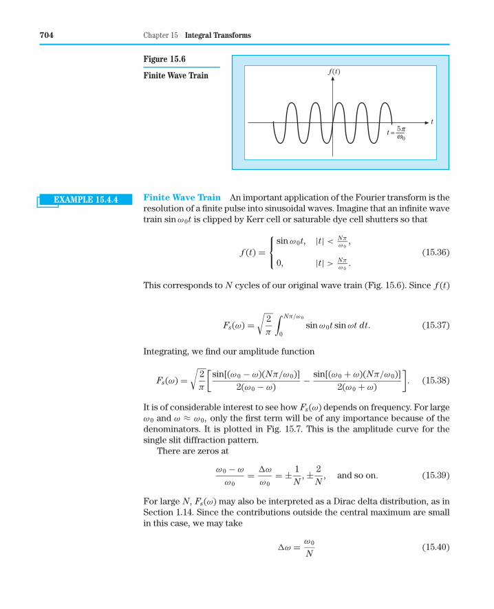
EXAMPLE 15.4.4 Finite Wave Train An important application of the Fourier transform is theresolution of a finite pulse into sinusoidal waves. Imagine that an infinite wavetrain sin ω0t is clipped by Kerr cell or saturable dye cell shutters so that
f (t) =
sin ω0t, |t| < Nπω 0
,
0, |t| > Nπω 0
.
(15.36)
This corresponds to N cycles of our original wave train (Fig. 15.6). Since f (t)is odd, we may use the Fourier sine transform [Eq. (15.33)] to obtain
Fs(ω) =√
2π
∫ Nπ/ω 0
0sin ω0t sin ωt dt. (15.37)
Integrating, we find our amplitude function
Fs(ω) =√
2π
[sin[(ω0 − ω)(Nπ/ω0)]
2(ω0 − ω)− sin[(ω0 + ω)(Nπ/ω0)]
2(ω0 + ω)
]. (15.38)
It is of considerable interest to see how Fs(ω) depends on frequency. For largeω0 and ω ≈ ω0, only the first term will be of any importance because of thedenominators. It is plotted in Fig. 15.7. This is the amplitude curve for thesingle slit diffraction pattern.
There are zeros at
ω0 − ω
ω0= �ω
ω0= ± 1
N, ± 2
N, and so on. (15.39)
For large N, Fs(ω) may also be interpreted as a Dirac delta distribution, as inSection 1.14. Since the contributions outside the central maximum are smallin this case, we may take
�ω = ω0
N(15.40)

15.4 Fourier Transforms---Inversion Theorem 705
Npw0
gs(w)
w =w 0
12p
w
Figure 15.7
Fourier Transformof Finite Wave Train
as a good measure of the spread in frequency of our wave pulse. Clearly, if N
is large (a long pulse), the frequency spread will be small. On the other hand, ifour pulse is clipped short (N is small), the frequency distribution will be widerand the secondary maxima are more important. ■
EXERCISES
15.4.1 The function
f (t) ={
1, |t| < 1
0, |t| > 1
is a symmetrical finite step function.(a) Find the Fc(ω), Fourier cosine transform of f (t).(b) Taking the inverse cosine transform, show that
f (t) = 2π
∫ ∞
0
sin ω cos ωt
ωdω.
(c) From part (b) show that
∫ ∞
0
sin ω cos ωt
ωdω =
0, |t| > 1,π4 , |t| = 1,π2 , |t| < 1.
15.4.2 Derive sine and cosine representations of δ(t − x) that are comparableto the exponential representation [Eq. (15.26)].
ANS.2π
∫ ∞
0sin ωt sin ωx dω,
2π
∫ ∞
0cos ωt cos ωx dω.
706 Chapter 15 Integral Transforms
15.4.3 In a resonant cavity, an electromagnetic oscillation of frequency ω0
dies out as
A(t) = A0e−ω 0t/2Qe−iω 0t, t > 0.
(Take A(t) = 0 for t < 0.)The parameter Q is a measure of the ratio of stored energy to energyloss per cycle. Calculate the frequency distribution of the oscillation,a∗(ω)a(ω), where a(ω) is the Fourier transform of A(t).Note. The larger Q is, the sharper your resonance line will be.
ANS. a∗(ω)a(ω) = A20
2π
1(ω − ω0)2 + (ω0/2Q)2
.
15.4.4 (a) Calculate the Fourier exponential transform of f (t) = tne−a|t| forn = 1, 2, 3.
(b) Calculate the inverse transform by employing the calculus ofresidues (Section 7.2).
15.5 Fourier Transform of Derivatives
Figure 15.1 outlines the overall technique of using Fourier transforms andinverse transforms to solve a problem. Here, we take an initial step in solving
a differential equation—obtaining the Fourier transform of a derivative.Using the exponential form, we determine that the Fourier transform of
f (t) is
F(ω) = 1√2π
∫ ∞
−∞f (t)eiωtdt, (15.41)
and for df (t)/dt
F1(ω) = 1√2π
∫ ∞
−∞
df (t)dt
eiωtdt. (15.42)
Integrating Eq. (15.42) by parts, we obtain
F1(ω) = eiωt
√2π
f (t)
∣∣∣∣∞
−∞− iω√
2π
∫ ∞
−∞f (t)eiωtdt. (15.43)
If f (t) vanishes4 as t → ±∞, we have
F1(ω) = −iωF(ω); (15.44)
that is, the transform of the derivative is (−iω) times the transform of theoriginal function. This may readily be generalized to the nth derivative to yield
Fn(ω) = (−iω)nF(ω), (15.45)
4Apart from cases such as Exercises 15.3.5 and 15.3.6, f (t) must vanish as t → ±∞ in order forthe Fourier transform of f (t) to exist.
15.5 Fourier Transform of Derivatives 707
provided all the integrated parts of Eq. (15.43) vanish as t → ±∞. This is thepower of the Fourier transform, the main reason it is so useful in solving (par-tial) differential equations. The operation of differentiation in coordinate
space has been replaced by a multiplication in ω space. Such propertiesof the kernel are the key in applications of integral transforms to solving ordi-nary differential equations (ODEs) and partial differential equations (PDEs),developed next.
EXAMPLE 15.5.1 Driven Harmonic Oscillator If we substitute the Fourier integral y(t) =1√2π
∫ ∞−∞ Y(ω)eiωtdt into the harmonic oscillator ODE d2 y
dt2 +�2 y = Acos(ω0t),where t is the time now, we obtain an algebraic equation for Y(ω) called theFourier transform of our solution y(t),
1√2π
∫ ∞
−∞Y(ω)(�2 − ω2)eiωtdω = A
2
∫ ∞
−∞eiωt[δ(ω − ω0) + δ(ω + ω0)]dω,
because differentiating twice corresponds to multiplying Y(ω) by (iω)2, andwe represent the driving term as a Fourier integral with the only frequencies±ω0. Upon comparing integrands, valid because the integrals are over thesame interval in the same variable ω (or, more rigorously, using the inverseFourier transform), we find
Y(ω) =√
π
2A
�2 − ω2[δ(ω − ω0) + δ(ω + ω0)].
The resulting integral,
y(t) = A
2
∫ ∞
−∞
eiωt
�2 − ω2[δ(ω − ω0) + δ(ω + ω0)]dω = A
�2 − ω20
cos(ω0t),
is the steady-state and particular solution of our inhomogeneous ODE. Notethat the assumption that the end points in the partially integrated term
in Eq. (15.43) do not contribute eliminates solutions of the homoge-
neous harmonic oscillator ODE (called transients in physics; undampedsin �t, cos �t solutions in our case).
Alternatively, we Fourier transform the ODE as follows:
1√2π
∫ ∞
−∞
(d2 y
dt2+ �2 y
)eiωtdt = A
2√
2π
∫ ∞
−∞(eiω 0t + e−iω 0t)eiωtdt
= A√
π2[δ(ω − ω0) + δ(ω + ω0)].
We integrate by parts twice,∫ ∞
−∞
d2 y
dt2eiωtdt = dy
dteiωt
∣∣∣∣∞
−∞− iω
∫ ∞
−∞
dy
dteiωtdt
= −iω
[yeiωt
∣∣∣∣∞
−∞− iω
∫ ∞
−∞yeiωtdt
]= −ω2
∫ ∞
−∞yeiωtdt,

708 Chapter 15 Integral Transforms
assuming that y(t) → 0 and dy(t)dt
→ 0 sufficiently fast, as t → ±∞. The resultof comparing integrands (using the inverse Fourier transform) is the same asbefore:
(�2 − ω2)Y(ω) =√
π
2A[δ(ω − ω0) + δ(ω + ω0)]. ■
Similarly, a PDE might become an ODE, such as the heat flow PDE consid-ered next.
EXAMPLE 15.5.2 Heat Flow PDE To illustrate the transformation of a PDE into an ODE, letus Fourier transform the heat flow partial differential equation
∂ψ
∂t= a2 ∂2ψ
∂x2,
where the solution ψ(x, t) is the temperature in space as a function of time.By substituting the Fourier integral solution
ψ(x, t) = 1√2π
∫ ∞
−∞�(ω, t)e−iωx dω,
this yields an ODE for the Fourier transform � of ψ,
∂�
∂t= −a2ω2�(ω, t),
in the time variable t. Alternatively and equivalently, apply the inverse Fouriertransform to each side of the heat PDE. Integrating, we obtain
ln � = −a2ω2t + ln C, or � = Ce−a2ω2t,
where the integration constant C may still depend on ω and, in general, isdetermined by initial conditions. Putting this solution back into our inverseFourier transform,
ψ(x, t) = 1√2π
∫ ∞
−∞C(ω)e−iωxe−a2ω2tdω,
yields a separation of the x and t variables. For simplicity, we here takeC ω-independent (assuming appropriate initial conditions) and integrate bycompleting the square in ω, as in Example 15.2.2, making appropriate changesof variables and parameters (a2 → a2t, ω → x, t → −ω). This yields theparticular solution of the heat flow PDE,
ψ(x, t) = C
a√
2texp
(− x2
4a2t
),
that appears as a clever guess in Section 16.2. In effect, we have shown that ψ
is the inverse Fourier transform of C exp(−a2ω2t). ■
EXAMPLE 15.5.3 Inversion of PDE Derive a Fourier integral for the Green’s function G0 ofPoisson’s PDE, which is a solution of
∇2G0(r, r′) = δ(r − r′).

15.5 Fourier Transform of Derivatives 709
Once G0 is known, the general solution of Poisson’s PDE
∇2� = −4πρ(r)
of electrostatics is given as
�(r) =∫
G0(r, r′)4πρ(r′)d3r′.
Applying ∇2 to � and using the PDE the Green’s function satisfies, we checkthat
∇2�(r) =∫
∇2G0(r, r′)4πρ(r′)d3r′ =∫
δ(r − r′)4πρ(r′)d3r′ = 4πρ(r).
Now we use Fourier transforms of the δ function and G0, writing
∇2∫
g0(p)eip·(r−r′) d3 p
(2π)3=
∫eip·(r−r′) d3 p
(2π)3.
Because the integrands of equal Fourier integrals must be the same (almost)everywhere, which follows from the inverse Fourier transform, and with
∇eip·(r−r′) = ipeip·(r−r′),
this yields −p2g0(p) = 1. Substituting this solution into the inverse Fouriertransform for G0 gives
G0(r, r′) = −∫
eip·(r−r′) d3 p
(2π)3p2= − 1
4π |r − r′| .
We can verify the last part of this result by applying ∇2 to G0 again and recallingfrom Chapter 1 that ∇2 1
|r−r′| = −4πδ(r − r′).The inverse Fourier transform can be evaluated using polar coordinates
exploiting the spherical symmetry of p2, similar to the charge form factor inExample 15.4.3 for a spherically symmetric charge density. For simplicity, wewrite R = r − r′ and call θ the angle between R and p so that∫
eip·R d3 p
p2=
∫ ∞
0dp
∫ 1
−1eipR cos θd cos θ
∫ 2π
0dϕ
= 2π
iR
∫ ∞
0
dp
peipR cos θ
∣∣∣∣1
cos θ=−1= 4π
R
∫ ∞
0
sin pR
pdp
= 4π
R
∫ ∞
0
sin pR
pRd(pR) = 2π2
R,
where θ and ϕ are the angles of p, and∫ ∞
0sin x
xdx = π
2 from Example 7.2.4.Dividing by −(2π)3, we obtain G0(R) = −1/(4π R), as claimed. An evaluationof this Fourier transform by contour integration is given in Example 16.3.2. ■
EXAMPLE 15.5.4 Wave Equation The Fourier transform technique may be used to advantagein handling PDEs with constant coefficients. To illustrate the technique further,let us derive a familiar expression of elementary physics. An infinitely long

710 Chapter 15 Integral Transforms
string is vibrating freely. The amplitude y of the (small) vibrations satisfies thewave equation
∂2 y
∂x2= 1
v2
∂2 y
∂t2. (15.46)
We shall assume an initial condition
y(x, 0) = f (x), (15.47)
where f is localized, that is, approaches zero at large x.
Applying our Fourier transform to both sides of our PDE [Eq. (15.46)]means multiplying by eiαx/
√2π and integrating over x according to
Y(α, t) = 1√2π
∫ ∞
−∞y(x, t)eiαxdx (15.48)
and using Eq. (15.43) for the second derivative. Note that the integrated partof ∂Y
∂xand ∂2Y
∂x 2 vanishes: The wave has not yet gone to ±∞, as it is propagatingforward in time, and there is no source at infinity [ f (±∞) = 0]. We obtain
∫ ∞
−∞
∂2 y(x, t)∂x2
eiαxdx = 1v2
∫ ∞
−∞
∂2 y(x, t)∂t2
eiαxdx (15.49)
or
(−iα)2Y(α, t) = 1v2
∂2Y(α, t)∂t2
. (15.50)
Since no derivatives with respect to α appear, Eq. (15.50) is actually an ODE—in fact, it is the linear oscillator equation. This transformation, from a PDE toan ODE, is a significant simplification. We solve Eq. (15.50) subject to the ap-propriate initial conditions. At t = 0, applying Eq. (15.47), Eq. (15.48) reducesto
Y(α, 0) = 1√2π
∫ ∞
−∞f (x)eiαxdx = F(α), (15.51)
where F(α) is the Fourier transform of the initial condition f (x). The generalsolution of Eq. (15.50) in exponential form is
Y(α, t) = F(α)e±ivαt. (15.52)
Using the inversion formula [Eq. (15.28)], we have
y(x, t) = 1√2π
∫ ∞
−∞Y(α, t)e−iαxdα, (15.53)
and, by Eq. (15.52),
y(x, t) = 1√2π
∫ ∞
−∞F(α)e−iα(x∓ vt)dα. (15.54)

15.5 Fourier Transform of Derivatives 711
Since f (x) is the Fourier inverse transform of F(α),
y(x, t) = f (x ∓ vt), (15.55)
corresponding to waves advancing in the +x- and −x-directions, respectively.The boundary condition of Eq. (15.47) is built into these particular linear
combinations of waves. ■
The accomplishment of the Fourier transform here deserves specialemphasis.
• The Fourier transform converts a PDE into an ODE, where the “degree oftranscendence” of the problem is reduced.
In Section 15.10, Laplace transforms are used to convert ODEs (with constantcoefficients) into algebraic equations. Again, the degree of transcendence isreduced. The problem is simplified, as outlined in Fig. 15.1.
EXERCISES
15.5.1 Equation (15.45) yields
F2(ω) = −ω2 F(ω)
for the Fourier transform of the second derivative of f (x). The con-dition f (x) → 0 for x → ±∞ may be relaxed slightly. Find the leastrestrictive condition for the preceding equation for F2(ω) to hold.
ANS.
[df (x)
dx− iω f (x)
]eiωx
∣∣∣∣∞
−∞= 0.
15.5.2 (a) Given that F(k) is the three-dimensional Fourier transform of f (r)and F1(k) is the three-dimensional Fourier transform of ∇ f (r),show that
F1(k) = (−ik)F(k).
This is a three-dimensional generalization of Eq. (15.45) for n = 1.(b) Show that the three-dimensional Fourier transform of ∇ ·∇ f (r) is
F2(k) = (−ik)2 F(k).
Note. Vector k is in the transform space. In Section 15.7, we shallhave hk = p, linear momentum.
15.5.3 Show ∫eik·(r−r′) d3k
(2π)3k2= 1
4π |r − r′|by contour integration in conjunction with the residue theorem.Hint. Use spherical polar coordinates in k-space.
712 Chapter 15 Integral Transforms
15.5.4 Solve the PDE∂y
∂t= ∂2 y
∂x2− a2 y
by Fourier transform, where y(x, t = 0) = 0, x > 0, y(x = 0, t) =f (t), t > 0, and a is a constant.
15.5.5 Show that the three-dimensional Fourier exponential transform ofa radially symmetric function may be rewritten as a Fourier sinetransform:
1(2π)3/2
∫ ∞
−∞f (r)eik·r d3x = 1
k
√2π
∫ ∞
−∞[r f (r)] sin kr dr.
15.6 Convolution Theorem
We employ convolutions to solve differential equations and to normalize mo-mentum wave functions.
Let us consider two functions f (x) and g(x) with Fourier transforms F(ω)and G(ω), respectively. We define the operation
f ∗ g ≡ 1√2π
∫ ∞
−∞g(y) f (x − y) dy (15.56)
as the convolution of the two functions f and g over the interval (−∞, ∞).This form of an integral appears in probability theory in the determination ofthe probability density of two random, independent variables. Our solution ofPoisson’s equation (i.e., the Coulomb potential) may be interpreted as a convo-lution of a charge distribution,ρ(r2), and a weighting function, (4πε0|r1−r2|)−1.In other works this is sometimes referred to as the Faltung, the German termfor “folding.”5 We now transform the integral in Eq. (15.56) by introducing theFourier transforms, interchanging the order of integration, and transformingg(y): ∫ ∞
−∞g(y) f (x − y)dy = 1√
2π
∫ ∞
−∞g(y)
∫ ∞
−∞F(ω)e−iω(x−y) dω dy
= 1√2π
∫ ∞
−∞F(ω)
[ ∫ ∞
−∞g(y)eiωy dy
]e−iωx dω
=∫ ∞
−∞F(ω)G(ω)e−iωxdω. (15.57)
Comparing with Eq. (15.56), this shows that
f ∗ g = L−1(FG).
In other words, the Fourier inverse transform of a product of Fourier trans-forms is the convolution of the original functions, f ∗ g.
5For f (y) = e−y, f (y) and f (x − y) are plotted in Fig. 15.8. Clearly, f (y) and f (x − y) are mirrorimages of each other in relation to the vertical line y = x/2; that is, we could generate f (x − y)by folding over f (y) on the line y = x/2.
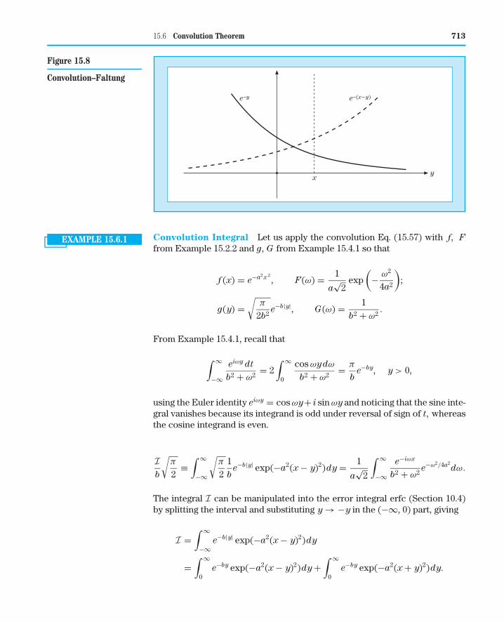
15.6 Convolution Theorem 713
yx
e–y e–(x–y)
Figure 15.8
Convolution--Faltung
EXAMPLE 15.6.1 Convolution Integral Let us apply the convolution Eq. (15.57) with f, F
from Example 15.2.2 and g, G from Example 15.4.1 so that
f (x) = e−a2x 2, F(ω) = 1
a√
2exp
(− ω2
4a2
);
g(y) =√
π
2b2e−b|y|, G(ω) = 1
b2 + ω2.
From Example 15.4.1, recall that
∫ ∞
−∞
eiωy dt
b2 + ω2= 2
∫ ∞
0
cos ωydω
b2 + ω2= π
be−by, y > 0,
using the Euler identity eiωy = cos ωy+ i sin ωy and noticing that the sine inte-gral vanishes because its integrand is odd under reversal of sign of t, whereasthe cosine integrand is even.
Now we apply the convolution formula [Eq. (15.57)]
Ib
√π
2≡
∫ ∞
−∞
√π
21b
e−b|y| exp(−a2(x − y)2)dy = 1
a√
2
∫ ∞
−∞
e−iωx
b2 + ω2e−ω2/4a2
dω.
The integral I can be manipulated into the error integral erfc (Section 10.4)by splitting the interval and substituting y → −y in the (−∞, 0) part, giving
I =∫ ∞
−∞e−b|y| exp(−a2(x − y)2)dy
=∫ ∞
0e−by exp(−a2(x − y)2)dy +
∫ ∞
0e−by exp(−a2(x + y)2)dy.
714 Chapter 15 Integral Transforms
Now we substitute ξ = y − x in the first integral and ξ = y + x in thesecond, yielding
I = e−bx
∫ ∞
−x
e−bξ−a2ξ 2dξ + ebx
∫ ∞
x
e−bξ−a2ξ 2dξ.
Completing the square in the exponent as in Example 15.2.2 using
a2ξ 2 + bξ = a2(
ξ + b
2a2
)2
− b2
4a2,
we obtain, with the substitution aη = ξ + b/2a2,
I = 1a
e−bx+b2/4a2∫ ∞
−ax+b/2a
e−η2dη + 1
aebx+b2/4a2
∫ ∞
ax+b/2a
e−η2dη
so that finally√
π
2b2I = π
2ab√
2eb2/4a2
[e−bx erfc
(b
2a−ax
)+ ebxerfc
(b
2a+ax
)]. (15.58)
Another example is provided by changing g(y) in the previous example tothe square pulse g(y) = 1, for |y| < 1 and zero elsewhere. Its Fourier transformis given in Example 15.2.1 as
G(ω) = 1√2π
∫ ∞
−∞g(y)eiωy dy =
√2π
sin ω
ω.
The convolution with f (x) takes the interesting form∫ 1
−1exp(−a2(x − y)2)dy = 1
a√
π
∫ ∞
−∞e−ω2/4a2 sin ω
ωe−iωxdω,
where the left-hand side can again be converted to a difference of errorintegrals
∫ 1
−1exp(−a2(x − y)2)dy =
√π
2a[erfc(−a(1 + x)) − erfc(a(1 − x))]. ■
EXAMPLE 15.6.2 Coulomb Potential by Convolution The Coulomb potential for an ex-tended charge distribution ρ of a composite system,
V (r) =∫
ρ(r′)|r − r′|d
3r′,
appears to be a three-dimensional case of a convolution integral. If we recallthe charge form factor GE as the Fourier transform of the charge density fromExample 15.4.3,
1(2π)3/2
∫ρ(r)eip·rd3r = GE(p2)
(2π)3/2,

15.6 Convolution Theorem 715
and 1/p2 as the Fourier transform of 1/|r − r′| from Example 15.5.3,
(2π)3/2
4π |r − r′| =∫
eip·(r−r′)
(2π)3/2p2d3 p,
being careful to include all normalizations, then we can apply the convolutiontheorem to obtain
V (r) =∫
ρ(r′)d3r′
|r − r′| = 4π
∫GE(p2)
p2e−ip·r d3 p
(2π)3. (15.59)
Let us now evaluate this result for the proton Example 15.4.3. This gives
V (r) = 4π
R21 − R2
∫ (R2
1
1 + p2 R21
− R2
1 + p2 R2
)e−ip·r
p2
d3 p
(2π)3
= 4π
R21 − R2
∫ [(− R2
1
1 + p2 R21
+ 1p2
)R2
1 − R2(
1p2
− R2
1 + p2 R2
)]
× e−ip·r d3 p
(2π)3
= R21
R21 − R2
(1r
− e−r/R1
r
)− R2
R21 − R2
(1r
− e−r/R
r
)
= 1r
[1 − 1
R21 − R2
(R2
1e−r/R1 − R2e−r/R)]
for the electrostatic potential, a pointlike Coulomb potential combined with aYukawa shape which remains finite as r → 0. ■
Parseval’s Relation
Results analogous to Eq. (15.57) may be derived for the Fourier sine and cosinetransforms (Exercises 15.6.1 and 15.6.2).
For the special case x = 0 in Eq. (15.57), we have∫ ∞
−∞F(ω)G(ω)dω =
∫ ∞
−∞f (−y)g(y)dy. (15.60)
Equation (15.60) and the corresponding sine and cosine convolutions are of-ten called Parseval’s relations by analogy with Parseval’s theorem for Fourierseries (Chapter 14, Exercise 14.4.2). However, the minus sign in −y suggeststhat modifications be tried. We now do this with g∗ instead of g using a differenttechnique.
The Parseval relation6,7∫ ∞
−∞F(ω)G∗(ω)dω =
∫ ∞
−∞f (t)g∗(t)dt (15.61)
6Note that all arguments are positive, in contrast to Eq. (15.60).7Some authors prefer to restrict Parseval’s name to series and refer to Eq. (15.61) as Rayleigh’stheorem.
716 Chapter 15 Integral Transforms
may be derived elegantly using the Dirac delta function representation [Eq.(15.26)]. We have∫ ∞
−∞f (t)g∗(t)dt =
∫ ∞
−∞
1√2π
∫ ∞
−∞F(ω)e−iωtdω · 1√
2π
∫ ∞
−∞G∗(x)eixtdx dt,
(15.62)
with attention to the complex conjugation in the G∗(x) to g∗(t) transform.Integrating over t first and using Eq. (15.26), we obtain∫ ∞
−∞f (t)g∗(t) dt =
∫ ∞
−∞F(ω)
∫ ∞
−∞G∗(x)δ(x − ω)dx dω
=∫ ∞
−∞F(ω)G∗(ω)dω, (15.63)
our desired Parseval relation. (The ∗ of complex conjugation can also be ap-plied to f and F instead.) If f (t) = g(t), then the integrals in the Parsevalrelation are normalization integrals (Section 9.4). Equation (15.63) guaranteesthat if a function f (t) is normalized to unity, its transform F(ω) is likewisenormalized to unity. This is extremely important in quantum mechanics, asdiscussed in the next section.
It may be shown that the Fourier transform is a unitary operation (in theHilbert space L2 of square integrable functions). The Parseval relation is areflection of this unitary property—analogous to Exercise 3.4.14 for matrices.
In Fraunhofer diffraction optics, the diffraction pattern (amplitude) ap-pears as the transform of the function describing the aperture (compareExample 15.2.1). With intensity proportional to the square of the amplitude, theParseval relation implies that the energy passing through the aperture seemsto be somewhere in the diffraction pattern—a statement of the conservationof energy.
Parseval’s relations may be developed independently of the inverse Fouriertransform and then used rigorously to derive the inverse transform. Details aregiven by Morse and Feshbach,8 Section 4.8 (see also Exercise 15.6.3).
EXAMPLE 15.6.3 Integral by Parseval’s Relation Evaluate the integral∫ ∞−∞
dω(a2+ω2)2 . We start
by recalling from Example 15.4.1 that
1√2π
∫ ∞
−∞
eiωxdω
a2 + ω2= 2√
π
∫ ∞
0
cos ωx dω
a2 + ω2=
√π
2a2e−ax, x > 0.
Next we apply Parseval’s relation to∫ ∞
−∞
dω
(a2 + ω2)2= π
2a2
∫ ∞
−∞e−2a|x|dx = π
a2
∫ ∞
0e−2axdx
= − π
2a3e−2ax
∣∣∣∣∞
0= π
2a3. ■
8 Morse, P. M., and Feshbach, H. (1953). Methods of Theoretical Physics. McGraw-Hill, New York.
15.6 Convolution Theorem 717
EXERCISES
15.6.1 Work out the convolution equation corresponding to Eq. (15.57) for(a) Fourier sine transforms
12
∫ ∞
0g(y)[ f (y + x) + f (y − x)]dy =
∫ ∞
0Fs(t)Gs(t) cos tx dt,
where f and g are odd functions.(b) Fourier cosine transforms
12
∫ ∞
0g(y)[ f (y + x) + f (|x − y|)]dy =
∫ ∞
0Fc(t)Gc(t) cos tx dt,
where f and g are even functions.
15.6.2 Show that for both Fourier sine and Fourier cosine transformsParseval’s relation has the form
∫ ∞
0F(t)G(t)dt =
∫ ∞
0f (y)g(y)dy.
15.6.3 Starting from Parseval’s relation [Eq. (15.61)], let g(y) = 1, 0 ≤ y ≤ α,and zero elsewhere. From this derive the Fourier inverse transform[Eq. (15.28)].Hint. Differentiate with respect to α.
15.6.4 Solve Poisson’s equation ∇2ψ(r) = −ρ(r)/ε0 by the following se-quence of operations:(a) Take the Fourier transform of both sides of this equation. Solve for
the Fourier transform of ψ(r).(b) Carry out the Fourier inverse transform by using a three-dimen-
sional analog of the convolution theorem [Eq. (15.57)].
15.6.5 With F(ω) and G(ω) the Fourier transforms of f (t) and g(t), respec-tively, show that
∫ ∞
−∞| f (t) − g(t)|2 dt =
∫ ∞
−∞|F(ω) − G(ω)|2 dω.
If g(t) is an approximation to f (t), the preceding relation indicatesthat the mean square deviation in ω-space is equal to the mean squaredeviation in t-space.
15.6.6 Use the Parseval relation to evaluate∫ ∞−∞
ω2dω(ω2+a2)2 .
Hint. Compare Example 15.4.2.
ANS.π
2a.
718 Chapter 15 Integral Transforms
15.7 Momentum Representation
In advanced mechanics and in quantum mechanics, linear momentum andspatial position occur on an equal footing. In this section, we start with theusual space distribution and derive the corresponding momentum distribu-tion. For the one-dimensional case, our wave function ψ(x), a solution of theSchrodinger wave equation, has the following properties:
1. ψ∗(x)ψ(x)dx is the probability of finding the quantum particle between x
and x + dx and
2.
∫ ∞
−∞ψ∗(x)ψ(x)dx = 1, (15.64)
corresponding to one particle (along the x-axis).In addition, we have
3. 〈x〉 =∫ ∞
−∞ψ∗(x)xψ(x)dx (15.65)
for the average position of the particle along the x-axis. This is often calledan expectation value.
We want a function g(p) that will give the same information about themomentum.
1. g∗(p)g(p)dp is the probability that our quantum particle has a momentumbetween p and p + dp.
2.
∫ ∞
−∞g∗(p)g(p)dp = 1. (15.66)
3. 〈p〉 =∫ ∞
−∞g∗(p)p g(p)dp. (15.67)
As subsequently shown, such a function is given by the Fourier transform ofour space function ψ(x). Specifically,9
g(p) = 1√2πh
∫ ∞
−∞ψ(x)e−ipx/hdx (15.68)
g∗(p) = 1√2πh
∫ ∞
−∞ψ∗(x)eipx/hdx. (15.69)
The corresponding three-dimensional momentum function is
g(p) = 1(2πh)3/2
∫ ∞∫−∞
∫ψ(r)e−ir·p/hd3r.
To verify Eqs. (15.68) and (15.69), let us check properties 2 and 3.
9The h may be avoided by using the wave number k, p = kh (and p = kh) so that
ϕ(k) = 1(2π)1/2
∫ψ(x)e−ikxdx.

15.7 Momentum Representation 719
Property 2, the normalization, is automatically satisfied as a Parsevalrelation [Eq. (15.61)]. If the space function ψ(x) is normalized to unity, themomentum function g(p) is also normalized to unity.
To check property 3, we must show that
〈p〉 =∫ ∞
−∞g∗(p)pg(p)dp =
∫ ∞
−∞ψ∗(x)
h
i
d
dxψ(x)dx, (15.70)
where (h/i)(d/dx) is the momentum operator in the space representation. Wereplace the momentum functions by Fourier transformed space functions, andthe first integral becomes
12πh
∫ ∞∫−∞
∫pe−ip(x−x′)/hψ∗(x′)ψ(x)dp dx′ dx. (15.71)
Now
pe−ip(x−x′)/h = d
dx
[− h
ie−ip(x−x′)/h
]. (15.72)
Substituting into Eq. (15.71) and integrating by parts, holding x′ and p constant,we obtain
〈p〉 =∫ ∞∫−∞
[1
2πh
∫ ∞
−∞e−ip(x−x′)/hdp
]· ψ∗(x′)
h
i
d
dxψ(x)dx′ dx. (15.73)
Here, we assume ψ(x) vanishes as x → ±∞, eliminating the integrated part.Again using the Dirac delta function [Eq. (15.23)], Eq. (15.73) reduces to Eq.(15.70) to verify our momentum representation. Note that technically we haveemployed the inverse Fourier transform in Eq. (15.68). This was chosen delib-erately to yield the proper sign in Eq. (15.73).
EXAMPLE 15.7.1 Hydrogen Atom The hydrogen atom ground state10 may be described bythe spatial wave function
ψ(r) =(
1
πa30
)1/2
e−r/a0 , (15.74)
with a0 being the Bohr radius, h2/me2. We now have a three-dimensional wavefunction. The transform corresponding to Eq. (15.68) is
g(p) = 1(2πh)3/2
∫ψ(r)e−ip·r/hd3r. (15.75)
Substituting Eq. (15.74) into Eq. (15.75) and using∫e−ar+ib·rd3r = 8πa
(a2 + b2)2, (15.76)
10For a momentum representation treatment of the hydrogen atom, l = 0 states, see Ivash, E. V.(1972). A momentum representation treatment of the hydrogen atom problem. Am. J. Phys. 40,1095.
720 Chapter 15 Integral Transforms
we obtain the hydrogenic momentum wave function
g(p) = 23/2
π
a3/20 h5/2
(a2
0 p2 + h2)2 . (15.77)
■
Such momentum functions have been found useful in problems such asCompton scattering from atomic electrons, the wavelength distribution of thescattered radiation, depending on the momentum distribution of the targetelectrons.
The relation between the ordinary space representation and the momentumrepresentation may be clarified by considering the basic commutation relationsof quantum mechanics. We go from a classical Hamiltonian to the Schrodingerequation by requiring that momentum p and position x not commute. Instead,we require that
[p, x] ≡ px − xp = −ih. (15.78)
For the multidimensional case, Eq. (15.78) is replaced by
[pk, xj] = −ihδkj. (15.79)
The Schrodinger (space) representation is obtained by using
(x): pk → −ih∂
∂xk
,
replacing the momentum by a partial space derivative. We see that
[p, x]ψ(x) = −ihψ(x). (15.80)
However, Eq. (15.78) can equally well be satisfied by using
(p): xj → ih∂
∂pj
.
This is the momentum representation. Then
[p, x]g(p) = −ihg(p). (15.81)
Hence, the representation (x) is not unique; (p) is an alternate possibility.In general, the Schrodinger representation (x) leading to the Schrodinger
equation is more convenient because the potential energy V is generally givenas a function of position V (x, y, z). The momentum representation (p) usu-ally leads to an integral equation. For an exception, consider the harmonicoscillator.
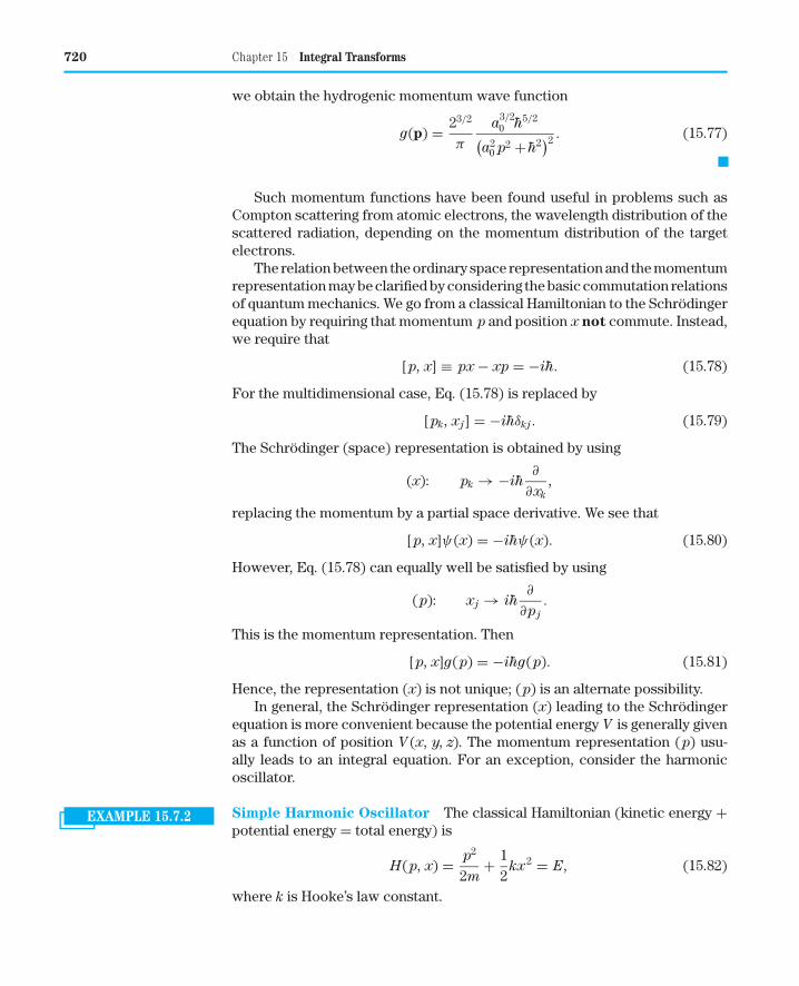
EXAMPLE 15.7.2 Simple Harmonic Oscillator The classical Hamiltonian (kinetic energy +potential energy = total energy) is
H(p, x) = p2
2m+ 1
2kx2 = E, (15.82)
where k is Hooke’s law constant.
15.7 Momentum Representation 721
In the Schrodinger representation we obtain
− h2
2m
d2ψ(x)dx2
+ 12
kx2ψ(x) = Eψ(x). (15.83)
For total energy E equal to√
(k/m)h/2, there is a solution (Section 13.1)
ψ(x) = e−(√
mk/(2h))x 2. (15.84)
The momentum representation leads to
p2
2mg(p) − h2k
2d2g(p)
dp2= Eg(p). (15.85)
Again, for
E =√
k
m
h
2(15.86)
the momentum wave equation (15.85) is satisfied by
g(p) = e−p2/(2h√
mk). (15.87)
Either representation, space or momentum (and an infinite number of otherpossibilities), may be used, depending on which is more convenient for theparticular problem under consideration.
The demonstration that g(p) is the momentum wave function correspond-ing to Eq. (15.83)—that it is the Fourier inverse transform of Eq. (15.83)—isleft as Exercise 15.7.3. ■
SUMMARY Fourier integrals derive their importance from the momentum space represen-tation in quantum mechanics. Fourier transformation of an ODE with constantcoefficients leads to a polynomial, and that of a PDE with constant coefficientsconverts the PDE to an ODE.
EXERCISES
15.7.1 A linear quantum oscillator in its ground state has a wave function
ψ(x) = a−1/2π−1/4e−x 2/2a2.
Show that the corresponding momentum function is
g(p) = a1/2π−1/4h−1/2e−a2 p2/2h2.
15.7.2 The nth excited state of the linear quantum oscillator is described by
ψn(x) = a−1/22−n/2π−1/4(n!)−1/2e−x 2/2a2Hn(x/a),
where Hn(x/a) is the nth Hermite polynomial (Section 13.1). As an ex-tension of Exercise 15.7.1, find the momentum function correspondingto ψn(x).
722 Chapter 15 Integral Transforms
Hint. ψn(x) may be represented by Ln+ψ0(x), where L+ is the raising
operator.
15.7.3 A free particle in quantum mechanics is described by a plane wave
ψk(x, t) = ei[kx−(hk2/2m)t].
Combining waves of adjacent momentum with an amplitude weightingfactor ϕ(k), we form a wave packet
�(x, t) =∫ ∞
−∞ϕ(k)ei[kx−(hk2/2m)t]dk.
(a) Solve for ϕ(k) given that
�(x, 0) = e−x 2/2a2.
(b) Using the known value of ϕ(k), integrate to get the explicit formof �(x, t). Note that this wave packet diffuses or spreads out withtime.
ANS. �(x, t) = e−{x 2/2[a2+(ih/m)t]}
[1 + (iht/ma2)]1/2.
Note. An interesting discussion of this problem from the evolutionoperator point of view is given by S. M. Blinder, Evolution of a Gaussianwave-packet. Am. J. Phys. 36, 525 (1968).
15.7.4 Find the time-dependent momentum wave function g(k, t) corres-ponding to �(x, t) of Exercise 15.7.3. Show that the momentum wavepacket g∗(k, t)g(k, t) is independent of time.
15.7.5 The deuteron (Example 9.1.2) may be described reasonably well witha Hulthen wave function
ψ(r) = A[e−αr − e−βr]/r,
with A, α, and β constants. Find g(p), the corresponding momentumwave function.Note. The Fourier transform may be rewritten as Fourier sine andcosine transforms or as a Laplace transform (Section 15.8).
15.7.6 The nuclear form factor F(k) and the charge distribution ρ(r) arethree-dimensional Fourier transforms of each other:
F(k) = 1(2π)3/2
∫ρ(r)eik·rd3r.
If the measured form factor is
F(k) = (2π)−3/2(
1 + k2
a2
)−1
,
find the corresponding charge distribution.
ANS. ρ(r) = a2
4π
e−ar
r.

15.7 Momentum Representation 723
15.7.7 Check the normalization of the hydrogen momentum wave function
g(p) = 23/2
π
a3/20 h5/2
(a2
0 p2 + h2)2
by direct evaluation of the integral∫g∗(p)g(p)d3 p.
15.7.8 With ψ(r) a wave function in ordinary space and ϕ(p) the correspond-ing momentum function, show that
(a)1
(2πh)3/2
∫rψ(r)e−ir·p/hd3r = ih∇pϕ(p),
(b)1
(2πh)3/2
∫r2ψ(r)e−ir·p/hd3r = (ih∇p)2ϕ(p).
Note. ∇p is the gradient in momentum space:
x∂
∂px
+ y∂
∂py
+ z∂
∂pz
.
These results may be extended to any positive integer power of r
and therefore to any (analytic) function that may be expanded as aMaclaurin series in r.
15.7.9 The ordinary space wave function ψ(r, t) satisfies the time-dependentSchrodinger equation
ih∂ψ(r, t)
∂t= − h2
2m∇2ψ + V (r)ψ.
Show that the corresponding time-dependent momentum wave func-tion satisfies the analogous equation
ih∂ϕ(p, t)
∂t= p2
2mϕ + V (ih∇p)ϕ.
Note. Assume that V (r) may be expressed by a Maclaurin series anduse Exercise 15.7.10. V (ih∇p) is the same function of the variable ih∇p
as V (r) is of the variable r.
15.7.10 The one-dimensional, time-independent Schrodinger equation is
− h2
2m
d2ψ(x)dx2
+ V (x)ψ(x) = Eψ(x).
For the special case of V (x) an analytic function of x, show that thecorresponding momentum wave equation is
V
(ih
d
dp
)g(p) + p2
2mg(p) = Eg(p).
Derive this momentum wave equation from the Fourier transform [Eq.(15.68)] and its inverse. Do not use the substitution x → ih(d/dp)directly.
724 Chapter 15 Integral Transforms
15.8 Laplace Transforms
Definition
The Laplace transform f (s) or L of a function F(t) is defined by11
f (s) = L {F(t)} = lima→∞
∫ a
0e−st F(t)dt =
∫ ∞
0e−st F(t)dt. (15.88)
A few comments on the existence of the integral are in order. The infiniteintegral of F(t), ∫ ∞
0F(t)dt,
need not exist. For instance, F(t) may diverge exponentially for large t.However, if there is some constant such that
|e−s0t F(t)| ≤ M, (15.89)
a positive constant for sufficiently large t, t > t0, the Laplace transform [Eq.(15.88)] will exist for s > s0; F(t) is said to be of exponential order. As acounterexample, F(t) = et2
does not satisfy the condition given by Eq. (15.89)and is not of exponential order. L{et2} does not exist.
The Laplace transform may also fail to exist because of a sufficiently strongsingularity in the function F(t) as t → 0; that is,∫ ∞
0e−sttn dt
diverges at the origin for n ≤ −1. The Laplace transform L {tn} does not existfor n ≤ −1.
Since for two functions F(t) and G(t), for which the integrals exist,
L {aF(t) + bG(t)} = aL {F(t)} + bL {G(t)} , (15.90)
the operation denoted by L is linear.
EXAMPLE 15.8.1 Elementary Functions To illustrate the Laplace transform, let us apply theoperation to some of the elementary functions. If
F(t) = 1, t > 0,
then
L {1} =∫ ∞
0e−stdt = 1
s, for s > 0. (15.91)
11This is sometimes called a one-sided Laplace transform; the integral from −∞ to +∞ is referredto as a two-sided Laplace transform. Some authors introduce an additional factor of s. This extra s
appears to have little advantage and continually gets in the way (see Additional Reading, Jeffreysand Jeffreys, Section 14.13). Generally, we take s to be real and positive. It is possible to have s
complex, provided �(s) > 0.
15.8 Laplace Transforms 725
Again, let
F(t) = ekt, t > 0.
The Laplace transform becomes
L{ekt} =∫ ∞
0e−stektdt = 1
s − k, for s > k, (15.92)
where the integral is finite. Using this relation, we obtain the Laplace transformof certain other functions. Since
cosh kt = 12
(ekt + e−kt), sinh kt = 12
(ekt − e−kt), (15.93)
we have
L {cosh kt} = 12
(1
s − k+ 1
s + k
)= s
s2 − k2,
(15.94)
L {sinh kt} = 12
(1
s − k− 1
s + k
)= k
s2 − k2,
both valid for s > k, where the integrals are finite. Because the results areanalytic functions of s, they may be continued analytically over the complexs-plane. This will prove useful for the inverse Laplace transform in Section15.12. We use the relations
cos kt = cosh ikt, sin kt = −i sinh ikt
in Eq. (15.94), with k replaced by ik, to find that the Laplace transforms
L {cos kt} = s
s2 + k2,
L {sin kt} = k
s2 + k2, (15.95)
both valid for s > 0, where the integrals are finite. Another derivation of thislast transform is given in the next section. Note that lims→0 L {sin kt} = 1/k.This suggests we assign a value of 1/k to the Laplace transform lims→0
∫ ∞0 e−st
sin kt dt.Finally, for F(t) = tn, we have
L{tn} =∫ ∞
0e−sttn dt,
which is the factorial function. Hence,
L{tn} = n!sn+1
, s > 0, n > −1. (15.96)
Note that in all these transforms we have the variable s in the denominator-negative powers of s. In particular, lims→∞ f (s) = 0. The significance of thispoint is that if f (s) involves positive powers of s, then lims→∞ f (s) → ∞ andno inverse transform exists. ■
726 Chapter 15 Integral Transforms
Inverse Transform
There is little importance to these operations, unless we can carry out theinverse transform as in Fourier transforms. That is, with
L {F(t)} = f (s),
then
L−1 { f (s)} = F(t).
Taken literally, this inverse transform is not unique. However, to the physicistand engineer the inverse operation may almost always be taken as unique inpractical problems.
The inverse transform can be determined in various ways. A table of trans-forms can be built up and used to carry out the inverse transformation exactlyas a table of logarithms can be used to look them up. The preceding transformsconstitute the beginnings of such a table. For a more complete set of Laplacetransforms, see AMS-55, Chapter 29. Employing partial fraction expansionsand various operational theorems, which are considered in succeeding sec-tions, facilitates use of the tables. There is some justification for suspectingthat these tables are probably of more value in solving textbook exercises thanin solving real-world problems.
A general technique for L−1 will be developed in Section 15.12 by usingthe calculus of residues. The difficulties and the possibilities of a numericalapproach—numerical inversion—are considered at the end of this section.
Partial Fraction Expansion
Utilization of a table of transforms (or inverse transforms) is facilitated byexpanding f (s) in partial fractions.
Frequently, f (s), our transform, occurs in the form g(s)/h(s), where g(s)and h(s) are polynomials with no common factors, g(s) being of lower degreethan h(s). If the factors of h(s) are all linear and distinct, then by the theory ofpartial fractions, we may write
f (s) = c1
s − a1+ c2
s − a2+ · · · + cn
s − an
, (15.97)
where the ci are independent of s. The ai are the roots of h(s). If any one ofthe roots (e.g., a1) is multiple (occurring m times), then f (s) has the form
f (s) = c1,m
(s − a1)m+ c1,m−1
(s − a1)m−1+ · · · + c1,1
s − a1+
n∑i=2
ci
s − ai
. (15.98)
Finally, if one of the factors is quadratic, (s2 + ps + q), the numerator, insteadof being a simple constant, will have the form
as + b
s2 + ps + q.
15.8 Laplace Transforms 727
There are various ways of determining the constants introduced. Forinstance, in Eq. (15.97) we may multiply through by (s − ai) and obtain
ci = lims→ai
(s − ai) f (s). (15.99)
In elementary cases a direct solution is often the easiest.
EXAMPLE 15.8.2 Partial Fraction Expansion Let
f (s) = k2
s(s2 + k2). (15.100)
We want to bring f (s) to the form
f (s) = c
s+ as + b
s2 + k2.
Putting the right side of this equation over a common denominator and equatinglike powers of s in the numerator, we obtain
k2
s(s2 + k2)= c(s2 + k2) + s(as + b)
s(s2 + k2), (15.101)
c + a = 0, s2; b = 0, s1; ck2 = k2, s0.
Solving these (s �= 0), we have
c = 1, b = 0, a = −1,
giving
f (s) = 1s
− s
s2 + k2(15.102)
and
L−1 { f (s)} = 1 − cos kt (15.103)
by Eqs. (15.91) and (15.95). ■
EXAMPLE 15.8.3 A Step Function As one application of Laplace transforms, consider theevaluation of
F(t) =∫ ∞
0
sin tx
xdx. (15.104)
Suppose we take the Laplace transform of this definite integral, which isfinite by virtue of the sign changes of the sine:
L{∫ ∞
0
sin tx
xdx
}=
∫ ∞
0e−st
∫ ∞
0
sin tx
xdx dt. (15.105)
728 Chapter 15 Integral Transforms
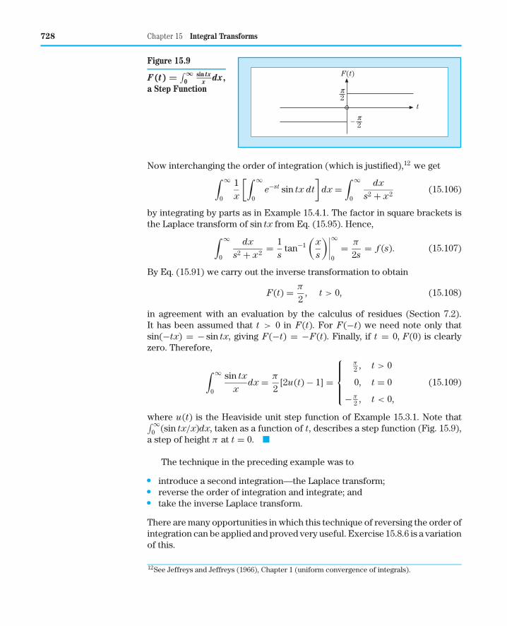
t
F(t)
p2
p2−
Figure 15.9
F (t) =∫ ∞
0sin tx
x dx ,a Step Function
Now interchanging the order of integration (which is justified),12 we get∫ ∞
0
1x
[∫ ∞
0e−st sin tx dt
]dx =
∫ ∞
0
dx
s2 + x2(15.106)
by integrating by parts as in Example 15.4.1. The factor in square brackets isthe Laplace transform of sin tx from Eq. (15.95). Hence,
∫ ∞
0
dx
s2 + x2= 1
stan−1
(x
s
)∣∣∣∣∞
0= π
2s= f (s). (15.107)
By Eq. (15.91) we carry out the inverse transformation to obtain
F(t) = π
2, t > 0, (15.108)
in agreement with an evaluation by the calculus of residues (Section 7.2).It has been assumed that t > 0 in F(t). For F(−t) we need note only thatsin(−tx) = − sin tx, giving F(−t) = −F(t). Finally, if t = 0, F(0) is clearlyzero. Therefore,
∫ ∞
0
sin tx
xdx = π
2[2u(t) − 1] =
π2 , t > 0
0, t = 0
−π2 , t < 0,
(15.109)
where u(t) is the Heaviside unit step function of Example 15.3.1. Note that∫ ∞0 (sin tx/x)dx, taken as a function of t, describes a step function (Fig. 15.9),
a step of height π at t = 0. ■
The technique in the preceding example was to
• introduce a second integration—the Laplace transform;• reverse the order of integration and integrate; and• take the inverse Laplace transform.
There are many opportunities in which this technique of reversing the order ofintegration can be applied and proved very useful. Exercise 15.8.6 is a variationof this.
12See Jeffreys and Jeffreys (1966), Chapter 1 (uniform convergence of integrals).
15.8 Laplace Transforms 729
Numerical Inversion
As an integration, the Laplace transform is a highly stable operation—stablein the sense that small fluctuations (or errors) in F(t) are averaged out inthe determination of the area under a curve. Also, the weighting factor, e−st,means that the behavior of F(t) at large t is effectively ignored—unless s
is small. As a result of these two effects, a large change in F(t) at large t
indicates a very small, perhaps insignificant, change in f (s). In contrast tothe Laplace transform operation, going from f (s) to F(t) is highly unstable.A minor change in f (s) may result in a wild variation of F(t). All significantfigures may disappear. In a matrix formulation, the matrix is ill conditionedwith respect to inversion.
There is no general, completely satisfactory numerical method for invert-ing Laplace transforms. However, if we are willing to restrict attention to rel-atively smooth functions, various possibilities open up. Bellman, Kalaba, andLockett13 convert the Laplace transform to a Mellin transform (x = e−t) anduse numerical quadrature based on shifted Legendre polynomials, P∗
n (x) =Pn(1−2x). The key step is analytic inversion of the resulting matrix. Krylov andSkoblya14 focus on the evaluation of the Bromwich integral (Section 15.12).As one technique, they replace the integrand with an interpolating polynomialof negative powers and integrate analytically.
EXERCISES
15.8.1 Prove that
lims→∞ sf (s) = lim
t→+0F(t).
Hint. Assume that F(t) can be expressed as F(t) = ∑∞n=0 antn.
15.8.2 Show that1π
lims→0L {cos xt} = δ(x).
15.8.3 Verify that
L{
cos at − cos bt
b2 − a2
}= s
(s2 + a2)(s2 + b2), a2 �= b2.
15.8.4 Using partial fraction expansions, show that
(a) L−1{
1(s + a)(s + b)
}= e−at − e−bt
b − a, a �= b.
(b) L−1{
s
(s + a)(s + b)
}= ae−at − be−bt
a − b, a �= b.
13Bellman, R., Kalaba, R. E., and Lockett, J. A. (1966). Numerical Inversion of the Laplace Trans-
forms. Elsevier, New York.14Krylov, V. I., and Skoblya, N. S. (1969). Handbook of Numerical Inversion of Laplace Transforms
(D. Louvish, Trans.). Israel Program for Scientific Translations, Jerusalem.
730 Chapter 15 Integral Transforms
15.8.5 Using partial fraction expansions, show that for a2 �= b2,
(a) L−1{
1(s2 + a2)(s2 + b2)
}= − 1
a2 − b2
{sin at
a− sin bt
b
},
(b) L−1{
s2
(s2 + a2)(s2 + b2)
}= 1
a2 − b2{a sin at − b sin bt}.
15.8.6 The electrostatic potential of a charged conducting disk is known tohave the general form (circular cylindrical coordinates)
�(ρ , z) =∫ ∞
0e−k|z| J0(kρ) f (k)dk,
with f (k) unknown. At large distances (z → ∞) the potential mustapproach the Coulomb potential Q/4πε0z. Show that
limk→0
f (k) = q
4πε0.
Hint. You may set ρ = 0 and assume a Maclaurin expansion of f (k) or,using e−kz, construct a delta sequence.
15.8.7 A function F(t) can be expanded in a power series (Maclaurin); that is,
F(t) =∞∑
n=0
antn.
Then
L {F(t)} =∫ ∞
0e−st
∞∑n=0
antn dt =∞∑
n=0
an
∫ ∞
0e−sttn dt.
Show that f (s), the Laplace transform of F(t), contains no powers of s
greater than s−1. Check your result by calculatingL {δ(t)} and commenton this fiasco.
15.9 Laplace Transform of Derivatives
Perhaps the main application of Laplace transforms is in converting differentialequations into simpler forms that may be solved more easily. It will be seen, forinstance, that coupled differential equations with constant coefficients
transform to simultaneous linear algebraic equations.Let us transform the first derivative of F(t):
L{F ′(t)} =∫ ∞
0e−st dF(t)
dtdt.
Integrating by parts, we obtain
L{F ′(t)} = e−st F(t)
∣∣∣∣∞
0+ s
∫ ∞
0e−st F(t)dt
= sL {F(t)} − F(0). (15.110)
15.9 Laplace Transform of Derivatives 731
Strictly speaking, F(0) = F(+0),15 and dF/dt is required to be at leastpiecewise continuous for 0 ≤ t < ∞. Naturally, both F(t) and its derivativemust be such that the integrals do not diverge. Incidentally, Eq. (15.110) pro-vides another proof of Exercise 15.8.7. An extension gives
L{F (2)(t)} = s2L {F(t)} − sF(+0) − F ′(+0), (15.111)
L{F (n)(t)} = snL{F(t)} − sn−1 F(+0) − · · · − F (n−1)(+0). (15.112)
The Laplace transform, like the Fourier transform, replaces differentiationwith multiplication. In the following examples, ODEs become algebraic equa-tions. Here is the power and the utility of the Laplace transform. When thecoefficients of the derivatives are not constant, Laplace transforms do notsimplify the ODE, as a rule.
Note how the initial conditions, F(+0), F ′(+0), and so on, are incorporatedinto the transform. Equation (15.111) may be used to derive L {sin kt}. We usethe identity
−k2 sin kt = d2
dt2sin kt. (15.113)
Then, applying the Laplace transform operation, we have
−k2L {sin kt} = L{
d2
dt2sin kt
}
= s2L {sin kt} − s sin(0) − d
dtsin kt|t=0. (15.114)
Since sin(0) = 0 and d/dt sin kt|t=0 = k,
L {sin kt} = k
s2 + k2, (15.115)
verifying Eq. (15.95).
EXAMPLE 15.9.1 Classical Harmonic Oscillator As a physical example, consider a mass m
oscillating under the influence of an ideal spring, spring constant k. Friction isneglected. Then Newton’s second law becomes
md2 X(t)
dt2+ kX(t) = 0. (15.116)
The initial conditions are taken to be
X(0) = X0, X′(0) = 0.
Applying the Laplace transform, we obtain
mL{
d2 X
dt2
}+ kL {X(t)} = 0, (15.117)
15Zero is approached from the positive side.
732 Chapter 15 Integral Transforms
and by use of Eq. (15.111) this becomes
ms2x(s) − msX0 + kx(s) = 0, (15.118)
x(s) = X0s
s2 + ω20
, with ω20 ≡ k
m. (15.119)
From Eq. (15.95) this is seen to be the transform of cos ω0t, which gives
X(t) = X0 cos ω0t, (15.120)
as expected. ■
Dirac Delta Function
For use with differential equations, one further transform is helpful—the Diracdelta function:16
L {δ(t − t0)} =∫ ∞
0e−stδ(t − t0)dt = e−st0 , for t0 ≥ 0, (15.121)
and for t0 = 0,
L {δ(t)} = 1, (15.122)
where, for Laplace transforms, δ(0) is interpreted as
δ(0) = limt0→0+
δ(t − t0). (15.123)
As an alternate method, δ(t) may be considered the limit as ε → 0 of F(t),where
F(t) =
0, t < 0,ε−1, 0 < t < ε,0, t > ε.
(15.124)
By direct calculation,
L {F(t)} = 1 − e−εs
εs. (15.125)
Taking the limit of the integral (instead of the integral of the limit), we have
limε→0L {F(t)} = 1
or Eq. (15.122)
L {δ(t)} = 1.
This delta function is frequently called the impulse function because it is souseful in describing impulsive forces, that is, forces lasting only a short time.
16Strictly speaking, the Dirac delta function is undefined. However, the integral over it is welldefined. This approach is developed in Section 1.14 using delta sequences.
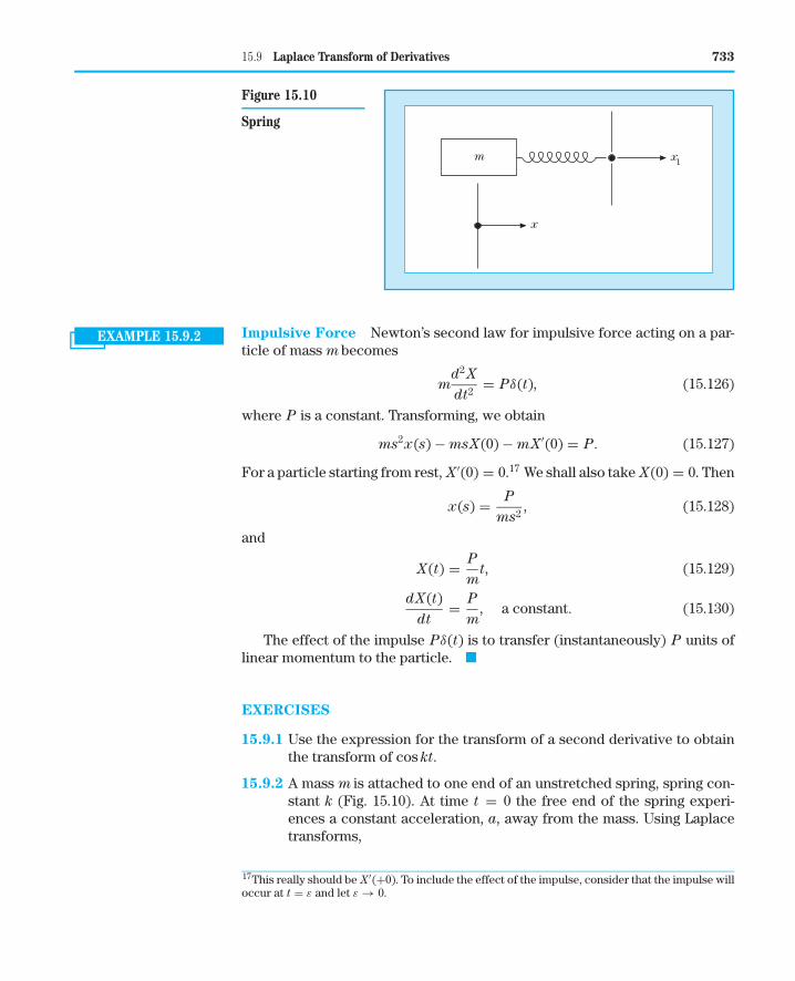
15.9 Laplace Transform of Derivatives 733
m
x
x1
Figure 15.10
Spring
EXAMPLE 15.9.2 Impulsive Force Newton’s second law for impulsive force acting on a par-ticle of mass m becomes
md2 X
dt2= Pδ(t), (15.126)
where P is a constant. Transforming, we obtain
ms2x(s) − msX(0) − mX′(0) = P. (15.127)
For a particle starting from rest, X′(0) = 0.17 We shall also take X(0) = 0. Then
x(s) = P
ms2, (15.128)
and
X(t) = P
mt, (15.129)
dX(t)dt
= P
m, a constant. (15.130)
The effect of the impulse Pδ(t) is to transfer (instantaneously) P units oflinear momentum to the particle. ■
EXERCISES
15.9.1 Use the expression for the transform of a second derivative to obtainthe transform of cos kt.
15.9.2 A mass m is attached to one end of an unstretched spring, spring con-stant k (Fig. 15.10). At time t = 0 the free end of the spring experi-ences a constant acceleration, a, away from the mass. Using Laplacetransforms,
17This really should be X′(+0). To include the effect of the impulse, consider that the impulse willoccur at t = ε and let ε → 0.

734 Chapter 15 Integral Transforms
(a) find the position x of m as a function of time; and(b) determine the limiting form of x(t) for small t.
ANS. (a) x = 12
at2 − a
ω2(1 − cos ωt), ω2 = k
m,
(b) x = aω2
4!t4, ωt � 1.
15.10 Other Properties
Substitution
If we replace the parameter s by s−a in the definition of the Laplace transform[Eq. (15.88)], we have
f (s − a) =∫ ∞
0e−(s−a)t F(t)dt =
∫ ∞
0e−steat F(t)dt
= L{eat F(t)}. (15.131)
Hence, the replacement of s with s − a corresponds to multiplying F(t) by eat
and conversely. This result can be used to good advantage in extending ourtable of transforms. From Eq. (15.95) we find immediately that
L{eat sin kt} = k
(s − a)2 + k2; (15.132)
also,
L{eat cos kt} = s − a
(s − a)2 + k2, s > a. (15.133)
EXAMPLE 15.10.1 Damped Oscillator These expressions are useful when we consider an os-cillating mass with damping proportional to the velocity. Equation (15.116),with such damping added, becomes
mX′′(t) + bX′(t) + kX(t) = 0, (15.134)
where b is a proportionality constant. Let us assume that the particle startsfrom rest at X(0) = X0, X′(0) = 0. The transformed equation is
m[s2x(s) − sX0] + b[sx(s) − X0] + kx(s) = 0 (15.135)
so that
x(s) = X0ms + b
ms2 + bs + k. (15.136)
This may be handled by completing the square of the denominator,
s2 + b
ms + k
m=
(s + b
2m
)2
+(
k
m− b2
4m2
). (15.137)
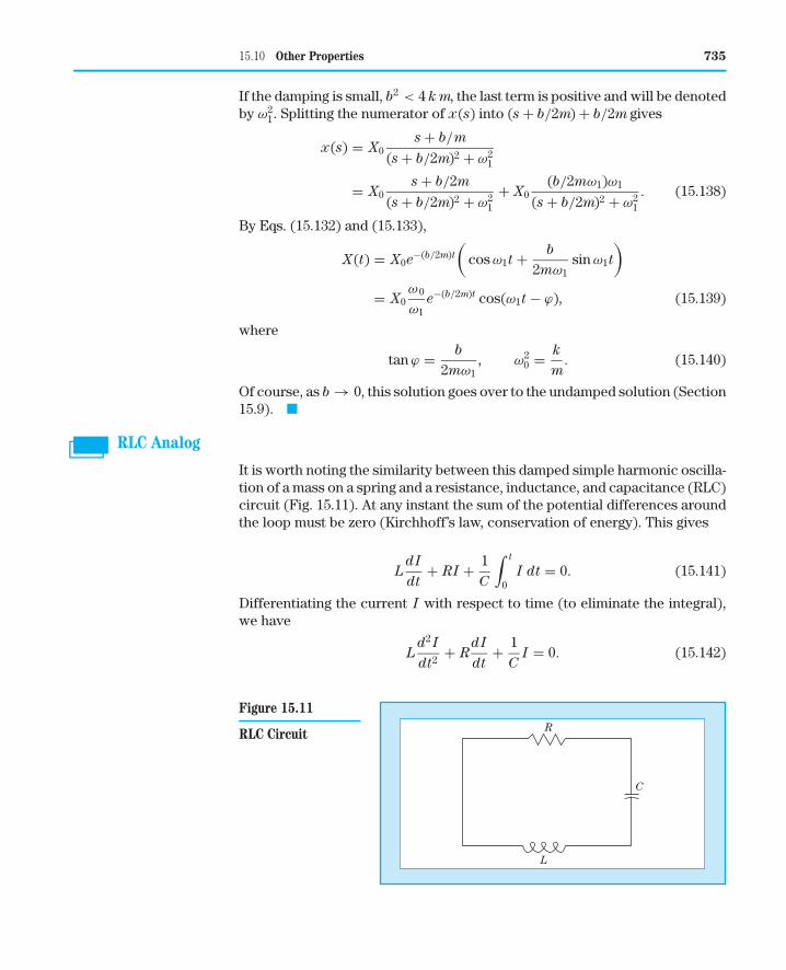
15.10 Other Properties 735
If the damping is small, b2 < 4 k m, the last term is positive and will be denotedby ω2
1. Splitting the numerator of x(s) into (s + b/2m) + b/2m gives
x(s) = X0s + b/m
(s + b/2m)2 + ω21
= X0s + b/2m
(s + b/2m)2 + ω21
+ X0(b/2mω1)ω1
(s + b/2m)2 + ω21
. (15.138)
By Eqs. (15.132) and (15.133),
X(t) = X0e−(b/2m)t(
cos ω1t + b
2mω1sin ω1t
)
= X0ω0
ω1e−(b/2m)t cos(ω1t − ϕ), (15.139)
where
tan ϕ = b
2mω1, ω2
0 = k
m. (15.140)
Of course, as b → 0, this solution goes over to the undamped solution (Section15.9). ■
RLC Analog
It is worth noting the similarity between this damped simple harmonic oscilla-tion of a mass on a spring and a resistance, inductance, and capacitance (RLC)circuit (Fig. 15.11). At any instant the sum of the potential differences aroundthe loop must be zero (Kirchhoff’s law, conservation of energy). This gives
LdI
dt+ RI + 1
C
∫ t
0I dt = 0. (15.141)
Differentiating the current I with respect to time (to eliminate the integral),we have
Ld2 I
dt2+ R
dI
dt+ 1
CI = 0. (15.142)
L
R
C
Figure 15.11
RLC Circuit
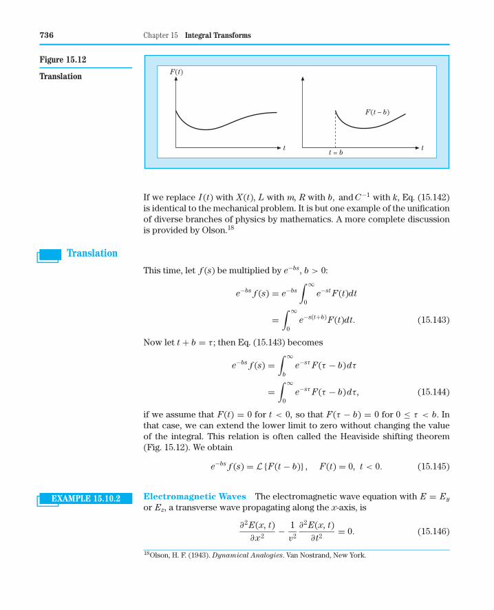
736 Chapter 15 Integral Transforms
t
F(t)
tt = b
F(t – b)
Figure 15.12
Translation
If we replace I(t) with X(t), L with m, R with b, and C−1 with k, Eq. (15.142)is identical to the mechanical problem. It is but one example of the unificationof diverse branches of physics by mathematics. A more complete discussionis provided by Olson.18
Translation
This time, let f (s) be multiplied by e−bs, b > 0:
e−bs f (s) = e−bs
∫ ∞
0e−st F(t)dt
=∫ ∞
0e−s(t+b)F(t)dt. (15.143)
Now let t + b = τ ; then Eq. (15.143) becomes
e−bs f (s) =∫ ∞
b
e−sτ F(τ − b)dτ
=∫ ∞
0e−sτ F(τ − b)dτ, (15.144)
if we assume that F(t) = 0 for t < 0, so that F(τ − b) = 0 for 0 ≤ τ < b. Inthat case, we can extend the lower limit to zero without changing the valueof the integral. This relation is often called the Heaviside shifting theorem(Fig. 15.12). We obtain
e−bs f (s) = L {F(t − b)} , F(t) = 0, t < 0. (15.145)
EXAMPLE 15.10.2 Electromagnetic Waves The electromagnetic wave equation with E = Ey
or Ez, a transverse wave propagating along the x-axis, is
∂2 E(x, t)∂x2
− 1v2
∂2 E(x, t)∂t2
= 0. (15.146)
18Olson, H. F. (1943). Dynamical Analogies. Van Nostrand, New York.
15.10 Other Properties 737
Transforming this equation with respect to t, we get
∂2
∂x2L {E(x, t)} − s2
v2L {E(x, t)} + s
v2E(x, 0) + 1
v2
∂E(x, t)∂t
∣∣∣∣t=0
= 0. (15.147)
If we have the initial conditions E(x, 0) = 0 and
∂E(x, t)∂t
∣∣∣∣t=0
= 0,
then
∂2
∂x2L {E(x, t)} = s2
v2L {E(x, t)} . (15.148)
The solution (of this ODE) is
L {E(x, t)} = c1e−(s/v)x + c2e+(s/v)x. (15.149)
The “constants” c1 and c2 are obtained by additional boundary conditions. Theyare constant with respect to x but may depend on s. If our wave remains finiteas x → ∞, L {E(x, t)} will also remain finite. Hence, c2 = 0.
If E(0, t) is denoted by F(t), then c1 = f (s) and
L {E(x, t)} = e−(s/v)x f (s). (15.150)
From the translation property [Eq. (15.144)] we find immediately that
E(x, t) =
F(t − x
v
), t ≥ x
v,
0, t < x
v,
(15.151)
which is consistent with our initial condition. Differentiation and substitutioninto Eq. (15.146) verifies Eq. (15.151). Our solution represents a wave (or pulse)moving in the positive x-direction with velocity v. Note that for x > vt theregion remains undisturbed; the pulse has not had time to get there. The otherindependent solution has c1 = 0 and corresponds to a signal propagated alongthe negative x-axis. ■
Derivative of a Transform
When F(t), which is at least piecewise continuous, and s are chosen so thate−st F(t) converges exponentially for large s, the integral
f (s) =∫ ∞
0e−st F(t)dt
is uniformly convergent and may be differentiated (under the integral sign)with respect to s. Then
f ′(s) =∫ ∞
0(−t)e−st F(t)dt = L {−tF(t)} . (15.152)
738 Chapter 15 Integral Transforms
Continuing this process, we obtain
f (n)(s) = L{(−t)nF(t)}. (15.153)
All the integrals so obtained will be uniformly convergent because of the de-creasing exponential behavior of e−st F(t).
This same technique may be applied to generate more transforms. Forexample,
L{ekt} =∫ ∞
0e−stektdt = 1
s − k, s > k. (15.154)
Differentiating with respect to s (or with respect to k), we obtain
L{tekt} = 1(s − k)2
, s > k. (15.155)
Integration of Transforms
Again, with F(t) at least piecewise continuous and x large enough, so thate−xt F(t) decreases exponentially (as x → ∞), the integral
f (x) =∫ ∞
0e−xt F(t)dt (15.156)
is uniformly convergent with respect to x. This justifies reversing the order ofintegration in the following equation:
∫ b
s
f (x)dx =∫ b
s
∫ ∞
0e−xt F(t)dt dx
=∫ ∞
0
F(t)t
(e−st − e−bt)dt, (15.157)
on integrating with respect to x. The lower limit s is chosen large enough sothat f (s) is within the region of uniform convergence. Now letting b → ∞, wehave ∫ ∞
s
f (x)dx =∫ ∞
0
F(t)t
e−stdt = L{
F(t)t
}, (15.158)
provided that F(t)/t is finite at t = 0 or diverges less strongly than t−1 [so thatL {F(t)/t} will exist].
Limits of Integration---Unit Step Function
The actual limits of integration for the Laplace transform may be specifiedwith the (Heaviside) unit step function
u(t − k) ={
0, t < k
1, t ≥ k.
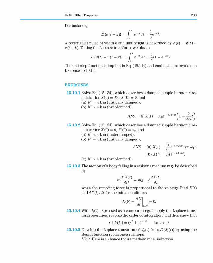
15.10 Other Properties 739
For instance,
L {u(t − k)} =∫ ∞
k
e−stdt = 1s
e−ks.
A rectangular pulse of width k and unit height is described by F(t) = u(t) −u(t − k). Taking the Laplace transform, we obtain
L {u(t) − u(t − k)} =∫ k
0e−st dt = 1
s(1 − e−ks).
The unit step function is implicit in Eq. (15.144) and could also be invoked inExercise 15.10.13.
EXERCISES
15.10.1 Solve Eq. (15.134), which describes a damped simple harmonic os-cillator for X(0) = X0, X′(0) = 0, and(a) b2 = 4 k m (critically damped),(b) b2 > 4 k m (overdamped).
ANS. (a) X(t) = X0e−(b/2m)t(
1 + b
2mt
).
15.10.2 Solve Eq. (15.134), which describes a damped simple harmonic os-cillator for X(0) = 0, X′(0) = v0, and(a) b2 < 4 k m (underdamped),(b) b2 = 4 k m (critically damped),
ANS. (a) X(t) = v0
ω1e−(b/2m)t sin ω1t,
(b) X(t) = v0te−(b/2m)t.(c) b2 > 4 k m (overdamped).
15.10.3 The motion of a body falling in a resisting medium may be describedby
md2 X(t)
dt2= mg − b
dX(t)dt
when the retarding force is proportional to the velocity. Find X(t)and dX(t)/dt for the initial conditions
X(0) = dX
dt
∣∣∣∣t=0
= 0.
15.10.4 With J0(t) expressed as a contour integral, apply the Laplace trans-form operation, reverse the order of integration, and thus show that
L {J0(t)} = (s2 + 1)−1/2, for s > 0.
15.10.5 Develop the Laplace transform of Jn(t) from L {J0(t)} by using theBessel function recurrence relations.Hint. Here is a chance to use mathematical induction.

740 Chapter 15 Integral Transforms
15.10.6 A calculation of the magnetic field of a circular current loop in cir-cular cylindrical coordinates leads to the integral∫ ∞
0e−kzkJ1(ka)dk, �(z) ≥ 0.
Show that this integral is equal to a/(z2 + a2)3/2.
15.10.7 Verify the following Laplace transforms:
(a) L{ j0(at)} = L{
sin at
at
}= 1
acot−1
( s
a
),
(b) L{y0(at)} does not exist.
15.10.8 Develop a Laplace transform solution of Laguerre’s ODE
tF ′′(t) + (1 − t)F ′(t) + nF(t) = 0.
Note that you need a derivative of a transform and a transform ofderivatives. Go as far as you can with n; then (and only then) setn = 0.
15.10.9 Show that the Laplace transform of the Laguerre polynomial Ln(at)is given by
L {Ln(at)} = (s − a)n
sn+1, s > 0.
15.10.10 Show that
L {E1(t)} = 1s
ln(s + 1), s > 0,
where
E1(t) =∫ ∞
t
e−τ
τdτ =
∫ ∞
1
e−xt
xdx.
E1(t) is the exponential–integral function.
15.10.11 (a) From Eq. (15.158) show that∫ ∞
0f (x)dx =
∫ ∞
0
F(t)t
dt,
provided the integrals exist.(b) From the preceding result show that∫ ∞
0
sin t
tdt = π
2,
in agreement with Eqs. (15.109) and (7.41).
15.10.12 (a) Show that
L{
sin kt
t
}= cot−1
(s
k
).

15.10 Other Properties 741
(b) Using this result (with k = 1), prove that
L{si(t)} = −1s
tan−1 s,
where
si(t) = −∫ ∞
t
sin x
xdx, the sine integral.
15.10.13 If F(t) is periodic (Fig. 15.13) with a period a so that F(t +a) = F(t)for all t ≥ 0, show that
L {F(t)} =∫ a
0 e−st F(t) dt
1 − e−as,
with the integration now over only the first period of F(t).
t3a
F(t)
2aa
Figure 15.13
Periodic Function
15.10.14 Find the Laplace transform of the square wave (period a) defined by
F(t) ={
1, 0 < t < a/2
0, a/2 < t < a.
ANS. f (s) = 1s
· 1 − e−as/2
1 − e−as.
15.10.15 Show that
(a) L{cosh at cos at} = s3
s4 + 4a4, (c) L{sinh at cos at} = as2 − 2a3
s4 + 4a4,
(b) L{cosh at sin at} = as2 + 2a3
s4 + 4a4, (d) L{sinh at sin at} = 2a2s
s4 + 4a4.
15.10.16 Show that(a) L−1{(s2 + a2)−2} = 1
2a3sin at − 1
2a2t cos at,
(b) L−1{s(s2 + a2)−2} = 12a
t sin at,
(c) L−1{s2(s2 + a2)−2} = 12a
sin at + 12
t cos at,
(d) L−1{s3(s2 + a2)−2} = cos at − a
2t sin at.
742 Chapter 15 Integral Transforms
y
x
31
2
(0, a) (a, a)
(a) (b)
(a, 0)
z(a, a)
(a, 0)t
31
2
Figure 15.14
Change of Variables:(a) xy-Plane and(b) zt-Plane
15.11 Convolution or Faltungs Theorem
One of the most important properties of the Laplace transform is that given bythe convolution or Faltungs theorem.19 We take two transforms
f1(s) = L{F1(t)} and f2(s) = L {F2(t)} (15.159)
and multiply them together. To avoid complications, when changing variables,we hold the upper limits finite:
f1(s) · f2(s) = lima→∞
∫ a
0e−sxF1(x)dx
∫ a−x
0e−syF2(y)dy. (15.160)
The upper limits are chosen so that the area of integration, shown in Fig. 15.14a,is the shaded triangle, not the square. Substituting x = t − z, y = z, the regionof integration is mapped into the triangle, shown in Fig. 15.14b. If we integrateover a square in the xy-plane, we have a parallelogram in the tz-plane, whichsimply adds complications. This modification is permissible because the twointegrands are assumed to decrease exponentially. In the limit a → ∞, theintegral over the unshaded triangle will give zero contribution. To verify themapping, map the vertices: t = x + y, z = y. Using Jacobians to transform theelement of area (Chapter 2), we have
dx dy =
∣∣∣∣∣∣∣∣
∂x
∂t
∂y
∂t
∂x
∂z
∂y
∂z
∣∣∣∣∣∣∣∣dt dz =
∣∣∣∣ 1 0−1 1
∣∣∣∣ dt dz (15.161)
19An alternate derivation employs the Bromwich integral (Section 15.12). This is Exercise 15.12.3.

15.11 Convolution or Faltungs Theorem 743
or dx dy = dt dz. With this substitution, Eq. (15.160) becomes
f1(s) · f2(s) = lima→∞
∫ a
0e−st
∫ t
0F1(t − z)F2(z)dz dt
= L{ ∫ t
0F1(t − z)F2(z)dz
}. (15.162)
For convenience this integral is represented by the symbol∫ t
0F1(t − z)F2(z)dz ≡ F1 ∗ F2, (15.163)
and referred to as the convolution, closely analogous to the Fourier convo-lution (Section 15.6). If we interchange f1 → f2 and F1 → F2 (or replacez → t − z), we find
F1 ∗ F2 = F2 ∗ F1, (15.164)
showing that the relation is symmetric.Carrying out the inverse transform, we also find
L−1 { f1(s) · f2(s)} =∫ t
0F1(t − z)F2(z)dz. (15.165)
This can be useful in the development of new transforms or as an alternativeto a partial fraction expansion. One immediate application is in the solution ofintegral equations. Since the upper limit t is variable, this Laplace convolutionis useful in treating Volterra integral equations. The Fourier convolution withfixed (infinite) limits would apply to Fredholm integral equations.
EXAMPLE 15.11.1 Driven Oscillator with Damping As an illustration of the use of the con-volution theorem, let us return to the mass mon a spring, with damping and adriving force F(t). The equation of motion [Eq. (15.134)] now becomes
mX′′(t) + bX′(t) + kX(t) = F(t). (15.166)
Initial conditions X(0) = 0, X′(0) = 0 are used to simplify this illustration, andthe transformed equation is
ms2x(s) + bs x(s) + kx(s) = f (s) (15.167)
or
x(s) = f (s)m
· 1
(s + b/2m)2 + ω21
, (15.168)
where ω21 ≡ k/m− b2/4m2, as before.
By the convolution theorem [Eq. (15.160) or Eq. (15.165)], and noting that
ω1
(s + b/2m)2 + ω21
= L(e−bt/2m sin ω1t),
744 Chapter 15 Integral Transforms
we have
X(t) = 1mω1
∫ t
0F(t − z)e−(b/2m)z sin ω1z dz. (15.169)
If the force is impulsive, F(t) = Pδ(t),20
X(t) = P
mω1e−(b/2m)t sin ω1t. (15.170)
P represents the momentum transferred by the impulse, and the constant P/m
takes the place of an initial velocity X′(0).If F(t) = F0 sin ωt, Eq. (15.168) may be used, but a partial fraction expan-
sion is perhaps more convenient. With
f (s) = F0ω
s2 + ω2,
Eq. (15.168) becomes
x(s) = F0ω
m· 1
s2 + ω2· 1
(s + b/2m)2 + ω21
= F0ω
m
[a′s + b′
s2 + ω2+ c′s + d′
(s + b/2m)2 + ω21
]. (15.171)
The coefficients a′, b′, c′, and d′ are independent of s. Direct calculation shows
− 1a′ = b
mω2 + m
b
(ω2
0 − ω2)2,
− 1b′ = −m
b
(ω2
0 − ω2)[ b
mω2 + m
b
(ω2
0 − ω2)2].
Since the c′s + d′ term will lead to exponentially decreasing terms (transients,as shown above the denominator is the Laplace transform of e−bt/2m sin ω1t),they will be discarded here. Carrying out the inverse operation, we find for thesteady-state solution
X(t) = F0[b2ω2 + m2
(ω2
0 − ω2)2]1/2 sin(ωt − ϕ), (15.172)
where
tan ϕ = bω
m(ω2
0 − ω2) .
Differentiating the denominator, we find that the amplitude has a maximumwhen
ω2 = ω20 − b2
2m2= ω2
1 − b2
4m2. (15.173)
20Note that δ(t) lies inside the interval [0, t].

15.11 Convolution or Faltungs Theorem 745
This is the resonance condition.21 At resonance the amplitude becomes F0/bω1,showing that the mass m goes into infinite oscillation at resonance if damp-ing is neglected (b = 0). It is worth noting that we have had three differentcharacteristic frequencies: resonance for forced oscillations, with damping,
ω22 = ω2
0 − b2
2m2;
free oscillation frequency, with damping,
ω21 = ω2
0 − b2
4m2;
and free oscillation frequency, no damping,
ω20 = k
m.
They coincide only if the damping is zero (b = 0).Returning to Eqs. (15.166) and (15.167), Eq. (15.167) is our ODE for the
response of a dynamical system to an arbitrary driving force. The final responseclearly depends on both the driving force and the characteristics of our system.This dual dependence is separated in the transform space. In Eq. (15.168) thetransform of the response (output) appears as the product of two factors, onedescribing the driving force (input) and the other describing the dynamicalsystem. This latter part, which modifies the input and yields the output, isoften called a transfer function. Specifically, [(s + b/2m)2 + ω2
1]−1 is thetransfer function corresponding to this damped oscillator. The concept of atransfer function is of great use in the field of servomechanisms. Often, thecharacteristics of a particular servomechanism are described by giving itstransfer function. The convolution theorem then yields the output signal for aparticular input signal. ■
EXERCISES
15.11.1 From the convolution theorem, show that
1s
f (s) = L{ ∫ t
0F(x)dx
},
where f (s) = L {F(t)}.15.11.2 Using the convolution integral, calculate
L−1{
s
(s2 + a2)(s2 + b2)
}, a2 �= b2.
15.11.3 An undamped oscillator is driven by a force F0 sin ωt. Find the dis-placement as a function of time. Notice that it is a linear combinationof two simple harmonic motions, one with the frequency of the driving
21The amplitude (squared) has the typical resonance denominator, the Lorentz line shape.
746 Chapter 15 Integral Transforms
force and one with the frequency ω0 of the free oscillator. (AssumeX(0) = X′(0) = 0.)
ANS. X(t) = F0/m
ω2 − ω20
(ω
ω0sin ω0t − sin ωt
).
15.12 Inverse Laplace Transform
Bromwich Integral
We now develop an expression for the inverse Laplace transform,L−1, appear-ing in the equation
F(t) = L−1{ f (s)}. (15.174)
One approach lies in the Fourier transform for which we know the inverserelation. There is a difficulty, however. Our Fourier transformable functionhad to satisfy the Dirichlet conditions. In particular, we required that
limω→∞ G(ω) = 0 (15.175)
so that the infinite integral would be well defined.22 Now we wish to treatfunctions, F(t), that may diverge exponentially. To surmount this difficulty,we extract an exponential factor, eγ t, from our (possibly) divergent Laplacefunction and write
F(t) = eγ tG(t). (15.176)
If F(t) diverges as eαt, we require γ to be greater than α so that G(t) will be
convergent. Now, with G(t) = 0 for t < 0 and otherwise suitably restrictedso that it may be represented by a Fourier transform [Eq. (15.20)],
G(t) = 12π
∫ ∞
−∞eiutdu
∫ ∞
0G(v)e−iuvdv. (15.177)
Using Eq. (15.177), we may rewrite Eq. (15.176) as
F(t) = eγ t
2π
∫ ∞
−∞eiutdu
∫ ∞
0F(v)e−γ ve−iuvdv. (15.178)
Now with the change of variable,
s = γ + iu, (15.179)
the integral over v is cast into the form of a Laplace transform∫ ∞
0F(v)e−svdv = f (s); (15.180)
22If delta functions are included, G(ω) may be a cosine. Although this does not satisfy Eq. (15.175),G(ω) is still bounded.
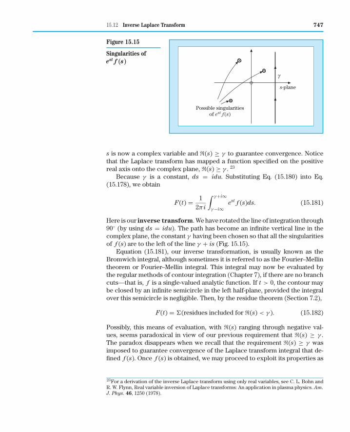
15.12 Inverse Laplace Transform 747
s-plane
g
Possible singularitiesof est f(s)
Figure 15.15
Singularities ofest f (s)
s is now a complex variable and �(s) ≥ γ to guarantee convergence. Noticethat the Laplace transform has mapped a function specified on the positivereal axis onto the complex plane, �(s) ≥ γ . 23
Because γ is a constant, ds = idu. Substituting Eq. (15.180) into Eq.(15.178), we obtain
F(t) = 12πi
∫ γ+i∞
γ−i∞est f (s)ds. (15.181)
Here is our inverse transform. We have rotated the line of integration through90◦ (by using ds = idu). The path has become an infinite vertical line in thecomplex plane, the constant γ having been chosen so that all the singularitiesof f (s) are to the left of the line γ + is (Fig. 15.15).
Equation (15.181), our inverse transformation, is usually known as theBromwich integral, although sometimes it is referred to as the Fourier–Mellintheorem or Fourier–Mellin integral. This integral may now be evaluated bythe regular methods of contour integration (Chapter 7), if there are no branchcuts—that is, f is a single-valued analytic function. If t > 0, the contour maybe closed by an infinite semicircle in the left half-plane, provided the integralover this semicircle is negligible. Then, by the residue theorem (Section 7.2),
F(t) = �(residues included for �(s) < γ ). (15.182)
Possibly, this means of evaluation, with �(s) ranging through negative val-ues, seems paradoxical in view of our previous requirement that �(s) ≥ γ .The paradox disappears when we recall that the requirement �(s) ≥ γ wasimposed to guarantee convergence of the Laplace transform integral that de-fined f (s). Once f (s) is obtained, we may proceed to exploit its properties as
23For a derivation of the inverse Laplace transform using only real variables, see C. L. Bohn andR. W. Flynn, Real variable inversion of Laplace transforms: An application in plasma physics. Am.
J. Phys. 46, 1250 (1978).
748 Chapter 15 Integral Transforms
an analytical function in the complex plane wherever we choose.24 In effect,we are employing analytic continuation to get L{F(t)} in the left half-plane ex-actly as the recurrence relation for the factorial function was used to extendthe Euler integral definition [Eq. (10.5)] to the left half-plane.
Perhaps two examples may clarify the evaluation of Eq. (15.182).
EXAMPLE 15.12.1 Inversion via Calculus of Residues If f (s) = a/(s2 − a2), then
est f (s) = aest
s2 − a2= aest
(s + a)(s − a). (15.183)
The residues may be found by using Exercise 7.1.1 or various other means. Thefirst step is to identify the singularities, the poles. Here, we have one simplepole at s = a and another simple pole at s = −a. By Exercise 7.1.1, the residueat s = a is (1
2 )eat and the residue at s = −a is (− 12 )e−at. Then
Residues =(
12
)(eat − e−at) = sinh at = F(t), (15.184)
in agreement with Eq. (15.94). ■
EXAMPLE 15.12.2 Another Inversion If
f (s) = 1 − e−as
s, a > 0,
then es(t−a) grows exponentially for t < a on the semicircle in the left-hands-plane so that contour integration and the residue theorem are not applicable.However, we can evaluate the integral explicitly as follows. We let γ → 0 andsubstitute s = iy so that
F(t) = 12πi
∫ γ+i∞
γ−i∞est f (s) = 1
2π
∫ ∞
−∞[eiyt − eit(t−a)]
dy
y. (15.185)
Using the Euler identity, only the sines survive that are odd in y, and we obtain
F(t) = 1π
∫ ∞
−∞
[sin ty
y− sin(t − a)y
y
]. (15.186)
If k > 0,∫ ∞
0sin ky
ydy gives π/2 and −π/2 if k < 0. As a consequence, F(t) = 0
if t > a > 0 and if t < 0. If 0 < t < a, then F(t) = 1. This can be writtencompactly in terms of the Heaviside unit step function u(t) as follows:
F(t) = u(t) − u(t − a) =
0, t < 0,
1, 0 < t < a,
0, t > a.
(15.187)
Thus, F(t) is a step function of unit height and length a (Fig. 15.16). ■
24In numerical work, f (s) may well be available only for discrete real, positive values of s. Thennumerical procedures are indicated. See Section 15.8 and the Krylov and Skoblya reference inAdditional Reading.
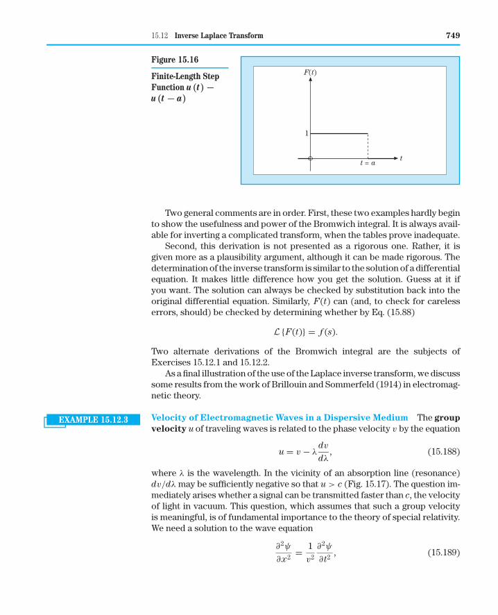
15.12 Inverse Laplace Transform 749
t = a
F(t)
1
t
Figure 15.16
Finite-Length StepFunction u(t) −u(t − a)
Two general comments are in order. First, these two examples hardly beginto show the usefulness and power of the Bromwich integral. It is always avail-able for inverting a complicated transform, when the tables prove inadequate.
Second, this derivation is not presented as a rigorous one. Rather, it isgiven more as a plausibility argument, although it can be made rigorous. Thedetermination of the inverse transform is similar to the solution of a differentialequation. It makes little difference how you get the solution. Guess at it ifyou want. The solution can always be checked by substitution back into theoriginal differential equation. Similarly, F(t) can (and, to check for carelesserrors, should) be checked by determining whether by Eq. (15.88)
L {F(t)} = f (s).
Two alternate derivations of the Bromwich integral are the subjects ofExercises 15.12.1 and 15.12.2.
As a final illustration of the use of the Laplace inverse transform, we discusssome results from the work of Brillouin and Sommerfeld (1914) in electromag-netic theory.
EXAMPLE 15.12.3 Velocity of Electromagnetic Waves in a Dispersive Medium The group
velocity u of traveling waves is related to the phase velocity v by the equation
u = v − λdv
dλ, (15.188)
where λ is the wavelength. In the vicinity of an absorption line (resonance)dv/dλ may be sufficiently negative so that u > c (Fig. 15.17). The question im-mediately arises whether a signal can be transmitted faster than c, the velocityof light in vacuum. This question, which assumes that such a group velocityis meaningful, is of fundamental importance to the theory of special relativity.We need a solution to the wave equation
∂2ψ
∂x2= 1
v2
∂2ψ
∂t2, (15.189)
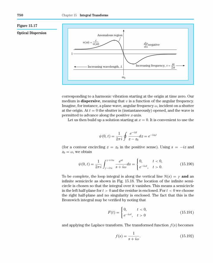
750 Chapter 15 Integral Transforms
w 0
1
Anomalous region
Increasing frequency, v =Increasing wavelength, l
negativedudl
w2p
n(w) =c
u(w)
Figure 15.17
Optical Dispersion
corresponding to a harmonic vibration starting at the origin at time zero. Ourmedium is dispersive, meaning that v is a function of the angular frequency.Imagine, for instance, a plane wave, angular frequency ω, incident on a shutterat the origin. At t = 0 the shutter is (instantaneously) opened, and the wave ispermitted to advance along the positive x-axis.
Let us then build up a solution starting at x = 0. It is convenient to use theCauchy integral formula [Eq. (6.37)],
ψ(0, t) = 12πi
∮e−izt
z − z0dz = e−iz0t
(for a contour encircling z = z0 in the positive sense). Using s = −iz andz0 = ω, we obtain
ψ(0, t) = 12πi
∫ γ+i∞
γ−i∞
est
s + iωds =
{0, t < 0,
e−iωt, t > 0.(15.190)
To be complete, the loop integral is along the vertical line �(s) = γ and aninfinite semicircle as shown in Fig. 15.18. The location of the infinite semi-circle is chosen so that the integral over it vanishes. This means a semicirclein the left half-plane for t > 0 and the residue is enclosed. For t < 0 we choosethe right half-plane and no singularity is enclosed. The fact that this is theBromwich integral may be verified by noting that
F(t) ={
0, t < 0,
e−iωt, t > 0(15.191)
and applying the Laplace transform. The transformed function f (s) becomes
f (s) = 1s + iω
. (15.192)
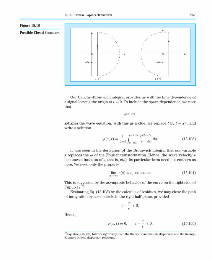
15.12 Inverse Laplace Transform 751
t < 0
–iw –iw
t > 0
Figure 15.18
Possible Closed Contours
Our Cauchy–Bromwich integral provides us with the time dependence ofa signal leaving the origin at t = 0. To include the space dependence, we notethat
es(t−x/v)
satisfies the wave equation. With this as a clue, we replace t by t − x/v andwrite a solution
ψ(x, t) = 12πi
∫ γ+i∞
γ−i∞
es(t−x/v)
s + iωds. (15.193)
It was seen in the derivation of the Bromwich integral that our variables replaces the ω of the Fourier transformation. Hence, the wave velocity v
becomes a function of s, that is, v(s). Its particular form need not concern ushere. We need only the property
lim|s|→∞
v(s) = c, constant. (15.194)
This is suggested by the asymptotic behavior of the curve on the right side ofFig. 15.17.25
Evaluating Eq. (15.193) by the calculus of residues, we may close the pathof integration by a semicircle in the right half-plane, provided
t − x
c< 0.
Hence,
ψ(x, t) = 0, t − x
c< 0, (15.195)
25Equation (15.193) follows rigorously from the theory of anomalous dispersion and the Kronig–Kramers optical dispersion relations.
752 Chapter 15 Integral Transforms
Table 15.1 Laplace Transform Operations
Operations Equation No.
Laplace transform f (s) = L{F(t)} =∫ ∞
0e−st F(t) dt (15.88)
Transform of derivative sf (s) − F(+0) = L{F ′(t)} (15.110)
s2 f (s) − sF(+0) − F ′(+0) = L{F ′′(t)} (15.111)
Transform of integral 1s
f (s) = L{ ∫ t
0F(x)dx
}Exercise 15.11.1
Substitution f (s − a) = L{eat F(t)} (15.131)
Translation e−bs f (s) = L{F(t − b)u(t − b)} (15.145)
Derivative of transform f (n)(s) = L{(−t)nF(t)} (15.153)
Integral of transform∫ ∞
s
f (x) dx = L{
F(t)t
}(15.158)
Convolution f1(s) f2(s) = L{ ∫ t
0F1(t − z)F2(z) dz
}(15.162)
Inverse transform, Bromwich integral1
2πi
∫ γ+i∞
γ−i∞est f (s)ds = F(t) (15.181)
which means that the velocity of our signal cannot exceed the velocity of lightin vacuum c. This simple but very significant result was extended by Som-merfeld and Brillouin to show just how the wave advanced in the dispersivemedium. ■
Summary: Inversion of Laplace Transform• Direct use of tables and references; use of partial fractions (Section 15.8)
and the operational theorems of Table 15.1.• Bromwich integral [Eq. (15.181)] and the calculus of residues.• Numerical inversion (Section 15.8) and references.
EXERCISES
15.12.1 Derive the Bromwich integral from Cauchy’s integral formula.Hint. Apply the inverse transform L−1 to
f (s) = 12πi
limα→∞
∫ γ+iα
γ−iα
f (z)s − z
dz,
where f (z) is analytic for �(z) ≥ γ .
15.12.2 Starting with
12πi
∫ γ+i∞
γ−i∞est f (s)ds,
show that by introducing
f (s) =∫ ∞
0e−szF(z)dz,
15.12 Inverse Laplace Transform 753
we can convert one integral into the Fourier representation of a Diracdelta function. From this, derive the inverse Laplace transform.
15.12.3 Derive the Laplace transformation convolution theorem by use ofthe Bromwich integral.
15.12.4 Find
L−1{
s
s2 − k2
}
(a) by a partial fraction expansion,(b) repeat using the Bromwich integral.
15.12.5 Find
L−1{
k2
s(s2 + k2)
}
(a) by using a partial fraction expansion,(b) repeat using the convolution theorem,(c) repeat using the Bromwich integral.
ANS. F(t) = 1 − cos kt.
15.12.6 Use the Bromwich integral to find the function whose transform isf (s) = s−1/2. Note that f (s) has a branch point at s = 0. The negativex-axis may be taken as a cut line.
ANS. F(t) = (π t)−1/2.
15.12.7 Evaluate the inverse Laplace transform
L−1 {(s2 − a2)−1/2}
by each of the following methods:(a) Expansion in a series and term-by-term inversion.(b) Direct evaluation of the Bromwich integral.(c) Change of variable in the Bromwich integral: s = (a/2)(z+ z−1).
15.12.8 Show that
L−1{
ln s
s
}= − ln t − γ ,
where γ = 0.5772 . . ., the Euler–Mascheroni constant.
15.12.9 Evaluate the Bromwich integral for
f (s) = s
(s2 + a2)2.
15.12.10 Heaviside expansion theorem. If the transform f (s) may be writtenas a ratio
f (s) = g(s)h(s)
,
754 Chapter 15 Integral Transforms
where g(s) and h(s) are analytic functions, with h(s) having simple,isolated zeros at s = si, show that
F(t) = L−1{
g(s)h(s)
}=
∑i
g(si)h′(si)
esit.
Hint. See Exercise 7.1.2.
15.12.11 Using the Bromwich integral, invert f (s) = s−2e−ks. Express F(t) =L−1 { f (s)} in terms of the (shifted) unit step function u(t − k).
ANS. F(t) = (t − k)u(t − k).
15.12.12 You have the following Laplace transform:
f (s) = 1(s + a)(s + b)
, a �= b.
Invert this transform by each of three methods:(a) partial fractions and use of tables;(b) convolution theorem; and(c) Bromwich integral.
ANS. F(t) = e−bt − e−at
a − b, a �= b.
Additional Reading
Champeney, D. C. (1973). Fourier Transforms and Their Physical Applica-
tions. Academic Press, New York. Fourier transforms are developed in acareful, easy to follow manner. Approximately 60% of the book is devotedto applications of interest in physics and engineering.
Erdelyi, A., Magnus, W., Oberhettinger, F., and Tricomi, F. G. (1954). Tables of
Integral Transforms. McGraw-Hill, New York. This text contains extensivetables of Fourier sine, cosine, and exponential transforms, Laplace andinverse Laplace transforms, Mellin and inverse Mellin transforms, Hankeltransforms, and other more specialized integral transforms.
Hanna, J. R. (1990). Fourier Series and Integrals of Boundary Value Prob-
lems. Wiley, Somerset, NJ. This book is a broad treatment of the Fouriersolution of boundary value problems. The concepts of convergence andcompleteness are given careful attention.
Jeffreys, H., and Jeffreys, B. S. (1972). Methods of Mathematical Physics, 3rded. Cambridge Univ. Press, Cambridge, UK.
Krylov, V. I., and Skoblya, N. S. (1969). Handbook of Numerical Inversion of
Laplace Transform. Israel Program for Scientific Translations, Jerusalem.Lepage, W. R. (1961). Complex Variables and the Laplace Transform for
Engineers. McGraw-Hill, New York. Reprinted, Dover, New York (1980). Acomplex variable analysis which is carefully developed and then appliedto Fourier and Laplace transforms. It is written to be read by students, butit is intended for the serious student.
McCollum, P. A., and Brown, B. F. (1965). Laplace Transform Tables and
Theorems. Holt, Rinehart and Winston, New York.
15.12 Inverse Laplace Transform 755
Miles, J. W. (1971). Integral Transforms in Applied Mathematics. CambridgeUniv. Press, Cambridge, UK. This is a brief but interesting and useful treat-ment for the advanced undergraduate. It emphasizes applications ratherthan abstract mathematical theory.
Papoulis, A. (1962). The Fourier Integral and Its Applications. McGraw-Hill,New York. This is a rigorous development of Fourier and Laplace trans-forms and has extensive applications in science and engineering.
Roberts, G. E., and Kaufman, H. (1966). Table of Laplace Transforms. Saun-ders, Philadelphia.
Sneddon, I. N. (1951). Fourier Transforms. McGraw-Hill, New York. Reprinted,Dover, New York (1995). A detailed comprehensive treatment, this book isloaded with applications to a wide variety of fields of modern and classicalphysics.
Sneddon, I. H. (1972). The Use of Integral Transforms. McGraw-Hill, NewYork. Written for students in science and engineering in terms they canunderstand, this book covers all the integral transforms mentioned in thischapter as well as in several others. Many applications are included.
Van der Pol, B., and Bremmer, H. (1987). Operational Calculus Based on the
Two-Sided Laplace Integral, 3rd ed. Cambridge Univ. Press, Cambridge,UK. Here is a development based on the integral range −∞ to +∞, ratherthan the useful 0 to ∞. Chapter 5 contains a detailed study of the Diracdelta function (impulse function).
Wolf, K. B. (1979). Integral Transforms in Science and Engineering. Plenum,New York. This book is a very comprehensive treatment of integral trans-forms and their applications.
Titchmarsh, E. C. (1937). Introduction to the Theory of Fourier Integrals, 2nded. Oxford Univ. Press, New York.


![1. Le serie di Fourier.web.inge.unige.it/DidRes/Analisi/ARG/18-Transforms.pdf · 1.Le serie di Fourier. È spesso utile saper rappresentare una funzione f : [p, p] !R mediante la](https://img.pdfslide.net/doc/110x75/5e7805ee5b260677f817a8fa/1-le-serie-di-1le-serie-di-fourier-spesso-utile-saper-rappresentare-una-funzione.jpg)


![Fast Modular Transforms* - University of Torontobor/Papers/fast-modular-transforms.pdf · 2013-07-22 · 368 BORODIN AND MOENCK Horowitz and Heindel [9] in investigating this question](https://img.pdfslide.net/doc/110x75/5cf66e2588c99374198c4829/fast-modular-transforms-university-of-borpapersfast-modular-transformspdf.jpg)