Embed Size (px)
Citation preview

Establishing some principles of human speech production throughtwo-dimensional computational models
Mauro Nicolao, Roger K. Moore
Speech and Hearing Group, Dept. Computer Science, University of Sheffield, [email protected], [email protected]
AbstractHuman speech production is often described as an optimi-
sation process, which tends to maximise the effectiveness of thecommunication process minimising the effort involved in theproduction.
The aim of this paper is to investigate this highly com-plex problem with two dimensionally reduced spaces corre-sponding to different computational models. Since the high-dimensional parameter space which usually describes such aproblem is often an issue in the optimal-behaviour computation,two-dimensional models are proposed. The first one analysesthe best trajectories visiting the proximity of a set of randomlychosen points. The second one explores the F1-F2 vowel spacetrying to maximise a set of likelihood functions describing somehuman production characteristics.
Even though such models need further development, somepreliminary correspondences can be observed with some ofthe elements described in the most popular theories for humanspeech production. For example, the distance between closecompetitors directly influences the best trajectory computationand, therefore, the effort needed to achieve the desired tasks.The trajectory planning is also controlled by the degree of mo-tivation selected to achieve the desired accuracy: the higher themotivation, the more the target must be addressed.Index Terms: human speech production model, reactive pro-duction model, hyper/hypo-articulation model, optimisationstrategies, trajectory planning.
1. IntroductionHuman talkers continuously adjust their speech productionwhile they are speaking. One of the first researchers who ob-served such behaviour was Lombard [1] almost a century agoand, after that study, several other theories have been proposed.Among others, Lindblom’s H&H (hypo-hyper) theory [2] af-firms that such modifications could be seen as a balancing pro-cess in which the talker tries to maximise the success of hiscommunication minimising the effort involved in production.
The hyper/hypo-articulated speech is intrinsically related tothe effort that the talker puts in his speech production and it isinfluenced by his motivation or by the contingencies which mayappear in the space. E. g. an utterance can be hyper-articulatedbecause the talker autonomously decides to make his productionextremely clear, because the environment forces him to com-pensate, or because it is imperative to avoid confusion betweenphonologically similar words.
Principles ruling such an optimisation are not completelyestablished. It might be the result of the continuous speechmonitoring by the talker in order to keep it as close as pos-sible to a desired phonetic plan [3]. The control loop could
be done assessing the acoustic outcome only, or with the so-matosensory system also to achieve prompter reactions to sud-den changes [4]. This process is often described as an attemptto satisfy the listener’s needs modelled inside the talker’s mindby a listener’s emulation [5]. The speech modification might bemodelled as the result of a previously learned modification ofthe speech quality (e.g. speech energy reallocation in the timeand frequency domain [6]) or, eventually, the product of the en-hancement/reduction of the acoustic distance between compet-ing phones in order to minimise possible misunderstandings. Inprevious experiments [7, 8, 9], it was shown that a data-drivenlinear transformation which controls such phonetic contrast canbe used to tune the degree of synthesised speech intelligibility.These results were found compatible with what most humansdo in adverse condition [10].
In order to establish some principles on how humans con-trol speech production, the use of proper computational modelsmight be useful. When parametric representation of speech isgiven, multidimensional acoustic space is also defined and ut-terances can be modelled as the parameter vector temporal evo-lution. If a likelihood function is also defined for every pointin such space, speech production turns into an optimisation pro-cess which aims to create the trajectory which navigates throughthe most likely points. It can be assumed that several things in-fluence such function: sequence of targets, trajectory evolution,competing-target density, possible external disturbances, etc.
Though, handling the great number of variables involvedin parametric speech representation is a overwhelming prob-lem in the investigation of optimal behaviour. E.g. a standardHMM-based speech synthesiser could have a vector dimensionof about 200 elements. In such highly complex spaces, a sim-ple visual representation of the problem, which can be crucialto assess the different strategies, is highly unlikely.
Motivated by these needs, two dimensionally-reducedspaces are introduced to be used as frameworks to test differentoptimal-trajectory search strategies. The future goal is to extendthem to the original multi-dimensional space. Even though theyare just simple descriptive models, their observation might, bysome extent, establish some fundamental principles still validin the high dimensional problem. Some minimum assumptionsare made in order to guarantee a certain degree of connection tothe real problem while complexity is reduced.
• A visual intuitive representation is helpful, therefore atwo-dimensional space should be chosen.
• The main goal in this trajectory planning should be tovisit a target sequence in a precise order.
• The simplified space should be defined by a set of pointsto identify targets and by some likelihood functions todescribe the area between them.

−600 −400 −200 0 200 400 600−400
−300
−200
−100
0
100
200
300
400
500
600
ph0
ph1
ph2
ph3
ph4
Figure 1: Example of two-dimensional space with 11 randompoints. The SZs are displayed with dash-lined circles. Fourtargets (ph1..4) and neutral position, ph0, are also shown.
• The optimal trajectory might vary at every step as func-tion of current position and of surrounding local space.
• The trajectory-evolution speed should not be fixed, butit should be dependant on the intensity of the stimulus:i.e. the farther the trajectory is from the target, the moreurgent the movement towards the it should be[11].
In the following sections, two models, which adopt theseguidelines, are proposed. Being intuitive and flexible spaces,many different strategies to navigate them can be used and somehints can be extended to real acoustic space.
2. First space: randomly-chosen pointsAs mentioned, reduction from a high-dimensional space is themost important simplification needed in order to better handleoptimal trajectory computation problem. Even if this space havea weak connection to the original acoustic space, it roughly re-minds of vowel space. Anyway, in this model more empha-sis was put on the navigation techniques of a two-dimensionalspace rather than on its relationship with the original acousticspace. Hence, the space is defined by a set of randomly-chosenpoints, {pn}, n = 1..N . Some of them are named as targets,{phl}, l = 1..L, while the N − L inactive points representobstacles for the trajectory, {xk}, k = 1..T , to avoid.
Trajectory goal is to visit every target in the right order. Ateach step, one target only is active and xk needs to go closer toit than to any other surrounding point in order to label currenttarget as visited. Hence, a circular area around each point pn
is defined. It is named Safe Zone for pn, or SZ(pn) because,when the trajectory is within this area, the related point, pn, canbe safely considered as visited. In an ideal vowel space, all thepoints in that area can be thought as set of recognisable realisa-tions of the phone pn. SZ(pn) radius is different for each pointand it is defined as half of the distance between pn and the clos-est among the other points which are also called competitors.An example of such space can be found in Figure 1.
The resulting trajectory is influenced by a weighting fac-tor which controls the SZ size. This controlling factor can beinterpreted as a measurement of the motivation involved in the
creation of the trajectory: i.e. how much the system allows formistakes among competitors. The number of steps needed bythe system to complete the path is therefore a direct measure-ment of this effort.
At the k-th step, one target only, phl, can be active. Allother positions consequently turn into competitors. The visitingorder is also important, therefore a target switching expressionis chosen to decide whether to switch the active target:
phk =
ph0 k ≤ 0phl if phk−1 = phl and xk 6∈ SZphlphl+1 if phk−1 = phl and xk ∈ SZphlph0 k ≥ T
(1)
where ph0 represents a neutral position and l is the target index.Two different strategies were tested to update the trajectory
in this space. The first and simplest one aims to find the shortestpath which visits each target. The second one forces the trajec-tory also to avoid competing SZs.
2.1. Minimising the distance to target
Minimising the distance between xk and target SZ is the firstcriterion used to compute the desired trajectory.
The resulting trajectory, {xk}, is composed by straightlines connecting the target SZs. Its evolution is described bythe following equation
xk+1 = xk + v(dk) ·∆xphk (2)
where ∆xphk = (phk − xk) is the vector identifying the tra-
jectory direction. The trajectory speed, v(.), is function of thedistance to target, dk = ‖phk − xk‖2. This relationship takesinspiration from Piron’s law [12], which states that mean humanresponse time to stimulus are quicker when this is stronger. Thelaw can be expressed by an exponential function. Consideringthe distance to target can be the stimulus, the speed function canbe expressed by
v(dk) = a1 · e(dk+
b1·b2b3
)2
(3)
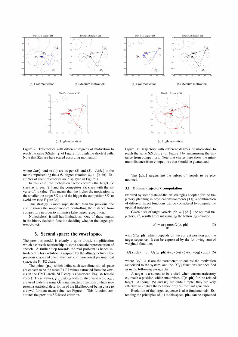
where a1, b1, b2, and b3 are empirical constants. Example ofresulting trajectories are displayed in Figure 2.
In Figure 2a, Figure 2b and Figure 2c, the SZs have dif-ferent sizes depending on the applied scaling factors. As al-ready mentioned, this value is related to the effort involved inthe trajectory creation. High motivation implies that the systemis making the effort to be more accurate in visiting targets andthis influences the correspondent SZ sizes.
This strategy represents a trajectory-computing algorithmcontrolled by an important factor in speech production such asmotivation, and it has clearly issues related to its simplicity.E.g. nothing prevents xk to go inside other-point SZs whileit is moving towards the target. This means that some pointscan be marked as visited even though they are not targets andthe system creates a different path from the desired one.
2.2. Maximising the distance from competitors
Since the previous strategy often creates trajectories which gointo competitor SZs before ending in the right target one, furtherconstraints are needed.
A correction factor, A(θk), is therefore applied to the di-rection vector in (2). The equation describing the evolution ofthe model becomes
xk+1 =
{xk + v(dk)∆xph
k if xk+1 6⊂ SZphj 6=k
xk + v(dk)A(θk)∆xphk if xk+1 ⊂ SZphj 6=k
(4)
−600 −400 −200 0 200 400 600−600
−400
−200
0
200
400
600
ph0
ph1
ph2
ph3
ph4
Effort (n. of steps) = 115
(a) Low motivation
−600 −400 −200 0 200 400 600−600
−400
−200
0
200
400
600
ph0
ph1
ph2
ph3
ph4
Effort (n. of steps) = 136
(b) Medium motivation
−600 −400 −200 0 200 400 600−600
−400
−200
0
200
400
600
ph0
ph1
ph2
ph3
ph4
Effort (n. of steps) = 167
(c) High motivation
Figure 2: Trajectories with different degrees of motivation toreach the same SZ(ph1..4) of Figure 1 through the shortest path.Note that SZs are here scaled according motivation.
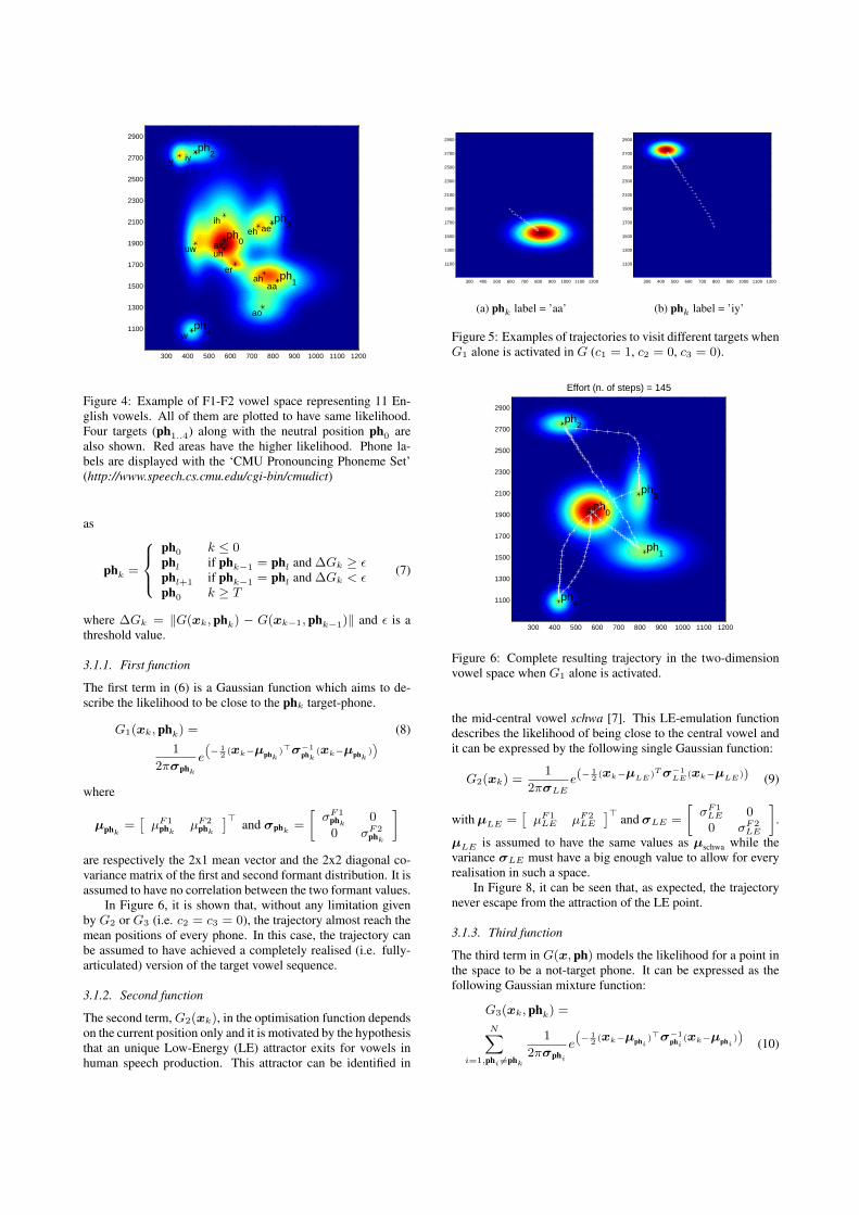
where ∆xphk and v(dk) are as per (2) and (3). A(θk) is the
matrix representing the a θk-degree rotation, θk ∈ [0, 2π]. Ex-amples of such trajectories are displayed in Figure 3.
In this case, the motivation factor controls the target SZsizes as in par. 2.1 and the competitor SZ sizes with the in-verse of its value. This means that the higher the motivation is,the smaller the target SZ is and the bigger the competitor SZs toavoid are (see Figure 3c).
This strategy is more sophisticated than the previous oneand it shows the importance of controlling the distance fromcompetitors in order to minimise false target recognition.
Nonetheless, it still has limitations. One of these standsin the binary decision function deciding whether the target phl
was visited.
3. Second space: the vowel spaceThe previous model is clearly a quite drastic simplificationwhich has weak relationship to some acoustic representation ofspeech. A further step towards the real problem is hence in-troduced. This evolution is inspired by the affinity between theprevious space and one of the most common vowel parametricalspace, the F1-F2 chart.
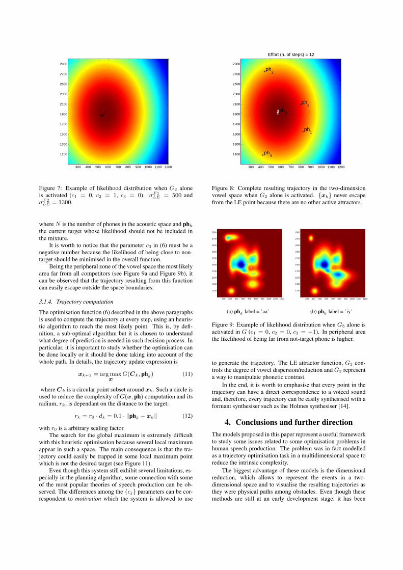
The points {pn} which define such two-dimensional spaceare chosen to be the mean F1-F2 values extracted from the vow-els in the CMU-arctic SLT corpus (American English femalevoice). These values, µpn
, along with relative variances, σpn ,are used to define some Gaussian mixture functions, which rep-resent a statistical description of the likelihood of being close toa vowel-formant mean value, see Figure 4. This function sub-stitutes the previous SZ-based criterion.
−600 −400 −200 0 200 400 600−600
−400
−200
0
200
400
600
ph0
ph1
ph2
ph3
ph4
Effort (n. of steps) = 135
(a) Low motivation
−600 −400 −200 0 200 400 600−600
−400
−200
0
200
400
600
ph0
ph1
ph2
ph3
ph4
Effort (n. of steps) = 165
(b) Medium motivation
−600 −400 −200 0 200 400 600−600
−400
−200
0
200
400
600
ph0
ph1
ph2
ph3
ph4
Effort (n. of steps) = 204
(c) High motivation
Figure 3: Trajectory with different degrees of motivation toreach the same SZ(ph1..4) of Figure 1 by maximising the dis-tance from competitors. Note that circles here show the mini-mum distance from competitors that should be guaranteed.
The {phl} targets are the subset of vowels to be pro-nounced.
3.1. Optimal trajectory computation
Inspired by some state-of-the-art strategies adopted for the tra-jectory planning in physical environments [13], a combinationof different target functions can be considered to compute theoptimal trajectory.
Given a set of target vowels, ph = {phl}, the optimal tra-jectory, x′, results from maximising the following equation
x′ = arg maxx
G(x, ph) (5)
with G(x, ph) which depends on the current position and thetarget sequence. It can be expressed by the following sum ofweighted functions
G(x, ph) = c1 ·G1(x, ph)+c2 ·G2(x)+c3 ·G3(x, ph) (6)
where {cj} > 0 are the parameters to control the motivationassociated to the system, and the {Gj} functions are specifiedas in the following paragraphs.
A target is assumed to be visited when current trajectoryxk reach a position which maximises G(x, ph) for the relatedtarget. Although (5) and (6) are quite simple, they are veryeffective to control the behaviour of this formant generator.
Evolution of the target sequence is also fundamentals. Ex-tending the principles of (1) in this space, phk can be expressed
aa
ae
ah
ao
ax
eh
er
ih
iy
uhuw
w
y
ph0
ph1
ph2
ph3
ph4
300 400 500 600 700 800 900 1000 1100 1200
1100
1300
1500
1700
1900
2100
2300
2500
2700
2900
Figure 4: Example of F1-F2 vowel space representing 11 En-glish vowels. All of them are plotted to have same likelihood.Four targets (ph1..4) along with the neutral position ph0 arealso shown. Red areas have the higher likelihood. Phone la-bels are displayed with the ‘CMU Pronouncing Phoneme Set’(http://www.speech.cs.cmu.edu/cgi-bin/cmudict)
as
phk =
ph0 k ≤ 0phl if phk−1 = phl and ∆Gk ≥ εphl+1 if phk−1 = phl and ∆Gk < εph0 k ≥ T
(7)
where ∆Gk = ‖G(xk, phk) − G(xk−1, phk−1)‖ and ε is athreshold value.
3.1.1. First function
The first term in (6) is a Gaussian function which aims to de-scribe the likelihood to be close to the phk target-phone.
G1(xk, phk) = (8)1
2πσphke
(− 1
2(xk−µphk
)>σ−1phk
(xk−µphk))
where
µphk=[µF1
phk µF2phk
]>and σphk =
[σF1
phk 0
0 σF2phk
]are respectively the 2x1 mean vector and the 2x2 diagonal co-variance matrix of the first and second formant distribution. It isassumed to have no correlation between the two formant values.
In Figure 6, it is shown that, without any limitation givenby G2 or G3 (i.e. c2 = c3 = 0), the trajectory almost reach themean positions of every phone. In this case, the trajectory canbe assumed to have achieved a completely realised (i.e. fully-articulated) version of the target vowel sequence.
3.1.2. Second function
The second term,G2(xk), in the optimisation function dependson the current position only and it is motivated by the hypothesisthat an unique Low-Energy (LE) attractor exits for vowels inhuman speech production. This attractor can be identified in
300 400 500 600 700 800 900 1000 1100 1200
1100
1300
1500
1700
1900
2100
2300
2500
2700
2900
(a) phk label = ’aa’
300 400 500 600 700 800 900 1000 1100 1200
1100
1300
1500
1700
1900
2100
2300
2500
2700
2900
(b) phk label = ’iy’
Figure 5: Examples of trajectories to visit different targets whenG1 alone is activated in G (c1 = 1, c2 = 0, c3 = 0).
ph0
ph1
ph2
ph3
ph4
Effort (n. of steps) = 145
300 400 500 600 700 800 900 1000 1100 1200
1100
1300
1500
1700
1900
2100
2300
2500
2700
2900
Figure 6: Complete resulting trajectory in the two-dimensionvowel space when G1 alone is activated.
the mid-central vowel schwa [7]. This LE-emulation functiondescribes the likelihood of being close to the central vowel andit can be expressed by the following single Gaussian function:
G2(xk) =1
2πσLEe(−
12(xk−µLE)Tσ−1
LE(xk−µLE)) (9)
withµLE =[µF1LE µF2
LE
]> andσLE =
[σF1LE 00 σF2
LE
].
µLE is assumed to have the same values as µschwa while thevariance σLE must have a big enough value to allow for everyrealisation in such a space.
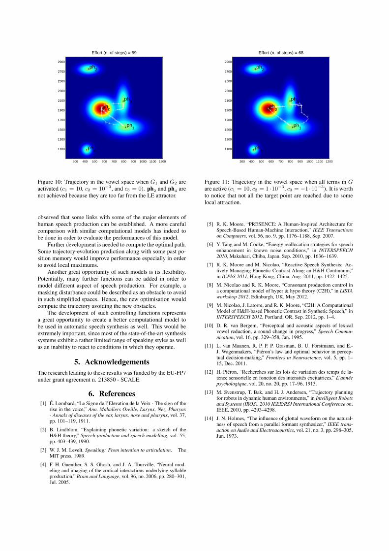
In Figure 8, it can be seen that, as expected, the trajectorynever escape from the attraction of the LE point.
3.1.3. Third function
The third term in G(x, ph) models the likelihood for a point inthe space to be a not-target phone. It can be expressed as thefollowing Gaussian mixture function:
G3(xk, phk) =
N∑i=1,phi 6=phk
1
2πσphie
(− 1
2(xk−µphi
)>σ−1phi
(xk−µphi))
(10)
ax
300 400 500 600 700 800 900 1000 1100 1200
1100
1300
1500
1700
1900
2100
2300
2500
2700
2900
Figure 7: Example of likelihood distribution when G2 aloneis activated (c1 = 0, c2 = 1, c3 = 0). σF1
LE = 500 andσF2LE = 1300.
whereN is the number of phones in the acoustic space and phk
the current target whose likelihood should not be included inthe mixture.
It is worth to notice that the parameter c3 in (6) must be anegative number because the likelihood of being close to non-target should be minimised in the overall function.
Being the peripheral zone of the vowel space the most likelyarea far from all competitors (see Figure 9a and Figure 9b), itcan be observed that the trajectory resulting from this functioncan easily escape outside the space boundaries.
3.1.4. Trajectory computation
The optimisation function (6) described in the above paragraphsis used to compute the trajectory at every step, using an heuris-tic algorithm to reach the most likely point. This is, by defi-nition, a sub-optimal algorithm but it is chosen to understandwhat degree of prediction is needed in such decision process. Inparticular, it is important to study whether the optimisation canbe done locally or it should be done taking into account of thewhole path. In details, the trajectory update expression is
xk+1 = arg maxx
G(Ck, phk) (11)
whereCk is a circular point subset around xk. Such a circle isused to reduce the complexity of G(x, ph) computation and itsradium, rk, is dependant on the distance to the target:
rk = r0 · dk = 0.1 · ‖phk − xk‖ (12)
with r0 is a arbitrary scaling factor.The search for the global maximum is extremely difficult
with this heuristic optimisation because several local maximumappear in such a space. The main consequence is that the tra-jectory could easily be trapped in some local maximum pointwhich is not the desired target (see Figure 11).
Even though this system still exhibit several limitations, es-pecially in the planning algorithm, some connection with someof the most popular theories of speech production can be ob-served. The differences among the {cj} parameters can be cor-respondent to motivation which the system is allowed to use
ph0
ph1
ph2
ph3
ph4
Effort (n. of steps) = 12
300 400 500 600 700 800 900 1000 1100 1200
1100
1300
1500
1700
1900
2100
2300
2500
2700
2900
Figure 8: Complete resulting trajectory in the two-dimensionvowel space when G2 alone is activated. {xk} never escapefrom the LE point because there are no other active attractors.
300 400 500 600 700 800 900 1000 1100 1200
1100
1300
1500
1700
1900
2100
2300
2500
2700
2900
(a) phk label = ’aa’
300 400 500 600 700 800 900 1000 1100 1200
1100
1300
1500
1700
1900
2100
2300
2500
2700
2900
(b) phk label = ’iy’
Figure 9: Example of likelihood distribution when G3 alone isactivated in G (c1 = 0, c2 = 0, c3 = −1). In peripheral areathe likelihood of being far from not-target phone is higher.
to generate the trajectory. The LE attractor function, G2 con-trols the degree of vowel dispersion/reduction and G3 representa way to manipulate phonetic contrast.
In the end, it is worth to emphasise that every point in thetrajectory can have a direct correspondence to a voiced soundand, therefore, every trajectory can be easily synthesised with aformant synthesiser such as the Holmes synthesiser [14].
4. Conclusions and further directionThe models proposed in this paper represent a useful frameworkto study some issues related to some optimisation problems inhuman speech production. The problem was in fact modelledas a trajectory optimisation task in a multidimensional space toreduce the intrinsic complexity.
The biggest advantage of these models is the dimensionalreduction, which allows to represent the events in a two-dimensional space and to visualise the resulting trajectories asthey were physical paths among obstacles. Even though thesemethods are still at an early development stage, it has been
ph0
ph1
ph2
ph3
ph4
Effort (n. of steps) = 59
300 400 500 600 700 800 900 1000 1100 1200
1100
1300
1500
1700
1900
2100
2300
2500
2700
2900
Figure 10: Trajectory in the vowel space when G1 and G2 areactivated (c1 = 10, c2 = 10−3, and c3 = 0). ph2 and ph4 arenot achieved because they are too far from the LE attractor.
observed that some links with some of the major elements ofhuman speech production can be established. A more carefulcomparison with similar computational models has indeed tobe done in order to evaluate the performances of this model.
Further development is needed to compute the optimal path.Some trajectory-evolution prediction along with some past po-sition memory would improve performance especially in orderto avoid local maximums.
Another great opportunity of such models is its flexibility.Potentially, many further functions can be added in order tomodel different aspect of speech production. For example, amasking disturbance could be described as an obstacle to avoidin such simplified spaces. Hence, the new optimisation wouldcompute the trajectory avoiding the new obstacles.
The development of such controlling functions representsa great opportunity to create a better computational model tobe used in automatic speech synthesis as well. This would beextremely important, since most of the state-of-the-art synthesissystems exhibit a rather limited range of speaking styles as wellas an inability to react to conditions in which they operate.
5. AcknowledgementsThe research leading to these results was funded by the EU-FP7under grant agreement n. 213850 - SCALE.
6. References[1] E. Lombard, “Le Signe de l’Elevation de la Voix - The sign of the
rise in the voice,” Ann. Maladiers Oreille, Larynx, Nez, Pharynx- Annals of diseases of the ear, larynx, nose and pharynx, vol. 37,pp. 101–119, 1911.
[2] B. Lindblom, “Explaining phonetic variation: a sketch of theH&H theory,” Speech production and speech modelling, vol. 55,pp. 403–439, 1990.
[3] W. J. M. Levelt, Speaking: From intention to articulation. TheMIT press, 1989.
[4] F. H. Guenther, S. S. Ghosh, and J. A. Tourville, “Neural mod-eling and imaging of the cortical interactions underlying syllableproduction,” Brain and Language, vol. 96, no. 2006, pp. 280–301,Jul. 2005.
ph0
ph1
ph2
ph3
ph4
Effort (n. of steps) = 68
300 400 500 600 700 800 900 1000 1100 1200
1100
1300
1500
1700
1900
2100
2300
2500
2700
2900
Figure 11: Trajectory in the vowel space when all terms in Gare active (c1 = 10, c2 = 1 ·10−3, c3 = −1 ·10−3). It is worthto notice that not all the target point are reached due to somelocal attraction.
[5] R. K. Moore, “PRESENCE: A Human-Inspired Architecture forSpeech-Based Human-Machine Interaction,” IEEE Transactionson Computers, vol. 56, no. 9, pp. 1176–1188, Sep. 2007.
[6] Y. Tang and M. Cooke, “Energy reallocation strategies for speechenhancement in known noise conditions,” in INTERSPEECH2010, Makuhari, Chiba, Japan, Sep. 2010, pp. 1636–1639.
[7] R. K. Moore and M. Nicolao, “Reactive Speech Synthesis: Ac-tively Managing Phonetic Contrast Along an H&H Continuum,”in ICPhS 2011, Hong Kong, China, Aug. 2011, pp. 1422–1425.
[8] M. Nicolao and R. K. Moore, “Consonant production control ina computational model of hyper & hypo theory (C2H),” in LISTAworkshop 2012, Edinburgh, UK, May 2012.
[9] M. Nicolao, J. Latorre, and R. K. Moore, “C2H: A ComputationalModel of H&H-based Phonetic Contrast in Synthetic Speech,” inINTERSPEECH 2012, Portland, OR, Sep. 2012, pp. 1–4.
[10] D. R. van Bergem, “Perceptual and acoustic aspects of lexicalvowel reduction, a sound change in progress,” Speech Commu-nication, vol. 16, pp. 329–358, Jan. 1995.
[11] L. van Maanen, R. P. P. P. Grasman, B. U. Forstmann, and E.-J. Wagenmakers, “Pieron’s law and optimal behavior in percep-tual decision-making,” Frontiers in Neuroscience, vol. 5, pp. 1–15, Dec. 2011.
[12] H. Pieron, “Recherches sur les lois de variation des temps de la-tence sensorielle en fonction des intensites excitatrices,” L’anneepsychologique, vol. 20, no. 20, pp. 17–96, 1913.
[13] M. Svenstrup, T. Bak, and H. J. Andersen, “Trajectory planningfor robots in dynamic human environments,” in Intelligent Robotsand Systems (IROS), 2010 IEEE/RSJ International Conference on.IEEE, 2010, pp. 4293–4298.
[14] J. N. Holmes, “The influence of glottal waveform on the natural-ness of speech from a parallel formant synthesizer,” IEEE trans-action on Audio and Electroacoustics, vol. 21, no. 3, pp. 298–305,Jun. 1973.