Natural Resources Canada

Ressources naturelles Canada

Canadian Forest Service

Service canadien des forêts

Development of a portable spectroscopic sensor to measure wood and fibre properties

in standing mountain pine beetle-attacked trees and decked logs

Esther Hsieh, Nelson Uy, Lars Wallbacks

Mountain Pine Beetle Initiative Working Paper 2006-16

Natural Resources Canada, Canadian Forest Service, Pacific Forestry Centre, 506 West Burnside Road, Victoria, BC V8Z 1M5

(250) 363-0600 • www.pfc.cfs.nrcan.gc.ca

cfs-scf.nrcan-rncan.gc.ca

- i -

Development of a portable spectroscopic sensor

to measure wood and fibre properties in standing

mountain pine beetle-attacked trees and decked logs

Esther Hsieh, Nelson Uy, Lars Wallbacks

Mountain Pine Beetle Initiative Working Paper 2006-16

Pulp and Paper Research Institute of Canada

3800 Wesbrook Mall, Vancouver BC, V6S 2L9

Mountain Pine Beetle Initiative PO # 8.14

Natural Resources Canada Canadian Forest Service Pacific Forestry Centre

506 West Burnside Road Victoria, British Columbia V8Z 1M5

Canada

2006

Her Majesty the Queen in Right of Canada 2006

Printed in Canada

- ii -

Library and Archives Canada Cataloguing in Publication

Hsieh, Esther

Development of a portable spectroscopic sensor to measure wood and fibre

properties in standing MPB attacked trees and decked logs / Esther Hsieh,

Nelson Uy, Lars Wallbacks.

(Mountain Pine Beetle Initiative working paper 2006-16)

Includes bibliographical references.

ISBN 0-662-44351-9

Cat. no.: Fo143-3/2006-16E

1. Lodgepole pine--Testing. 2. Lodgepole pine--Diseases and pests.

3. Mountain pine beetle. 4. Near infrared spectroscopy. I. Uy, Nelson II.

Wallbacks, Lars III. Pacific Forestry Centre IV. Title. V. Series.

SB945.M78H74 2006 634.9'7516768 C2006-980258-0

- iii -

Abstract

A visible-near-infrared (vis-NIR) spectrometer was used to develop a unique, fast-scanning and field-portable tool to quantify parameters of relevance to mountain pine beetle infested standing lodgepole pines and decked logs. Three calibration models to simultaneously predict moisture, density, blue stain and decay were developed for three different applications; 1) to measure wood cores in the laboratory 2) to obtain field measurements on standing trees 3) to measure decked logs. All calibration models were validated and the results demonstrate that vis-NIR can be used to measure moisture, blue stain and decay with high accuracy. Density trends can also be measured using vis-NIR spectroscopy, but with less accuracy than standard laboratory methods. Of the three models, the calibration for decked logs produced the smallest errors due to the larger measuring spot size and the superior optical design of the contact probe used to collect the data. Keywords: Mountain Pine Beetle, Blue Stain, Spectrometry, Spectroscopy, Visible, NIR, Near-Infrared, Moisture, Decay, Density, Measurements, Colour, Field Testing

Résumé

Un spectromètre visible et à proche infrarouge a permis de mettre au point un outil unique, à balayage rapide et portable pour quantifier les paramètres pertinents de billes empilées et d’arbres sur pied de pin tordu. Trois modèles d’étalonnage ont été élaborés pour prédire simultanément la présence d’humidité, la densité, le bleuissement et la pourriture dans le cadre de trois applications : 1) mesures sur des carottes de bois en laboratoire ; 2) mesures sur le terrain à partir d’arbres sur pied ; 3) mesures sur des billots empilés. Les modèles d’étalonnage ont été validés et les résultats obtenus font la preuve que la spectrométrie visible et à proche infrarouge permet de mesurer le degré d’humidité, le bleuissement et la pourriture avec une grande précision. La spectrométrie visible et à infrarouge permet aussi de mesurer l’évolution de la densité, mais avec moins de précision que les méthodes de laboratoire classiques. Des trois modèles, l'étalonnage des billots empilés affichait les erreurs les moins grandes en raison de la grandeur du point de mesure et de la conception optique supérieure de la sonde de contact servant à la collecte des données.

Mots-clés : Dendroctone du pin ponderosa, bleuissement, spectrométrie, spectroscopie, visible, proche infrarouge, humidité, pourriture, densité, mesures, couleur, essais sur le terrain

- iv -

Contents

1 Introduction .................................................................................................................... 1

2 Materials and Methods.................................................................................................... 1 2.1 Spectrometer hardware........................................................................................ 1 2.2 Field Sampling.................................................................................................... 5 2.3 Laboratory Measurements ................................................................................... 6 2.4 Calibrations......................................................................................................... 8

3 Results and Discussion ................................................................................................... 8 3.1 Models Developed on Wood Core Models with Straight Probe ........................... 8 3.2 Field Model Developed on Standing Tres with Right Angle Reflectance

Probe..................................................................................................................17 3.3 Model Developed for Decked Logs using Contact Probe ....................................22

4 Conclusions ..................................................................................................................29

5 Acknowledgements........................................................................................................29

6 Cited Literature..............................................................................................................30

7 Appendix ......................................................................................................................31

- 1 -

1 Introduction

The mountain pine beetle infestation in BC has resulted in a wood mixture that heavily favours attacked lodgepole pine trees. Foresters and field workers generally classify these infested lodgepole pine trees based on external characteristics such as the state of their needles. Green trees, generally 0-1 year since attack, are trees that can be still alive with green needles. Red trees, generally 2 - 4 years since attack, are dead trees with red needles and grey trees, generally 5 years and older, have lost their needles. Bark level and branches are also age indicators for grey stage trees, Thrower J.S., et al.). While visual indicators can be used to estimate the age of a tree or tree stand since attack, it is not a reliable predictor of the wood and fibre quality and therefore the true log value. Moisture content, blue stain, decay content and basic density are important determinants of the beetle infested wood end-use and hence wood valuation. Currently, the industry methods for measuring all four of these variables are time consuming, and because they are laboratory methods, this critical data cannot be obtained in a timely fashion to ensure that the end-use is considered when stands are harvested. The purpose of this research initiative was to develop models using vis-NIR spectroscopy on a portable analyzer to measure these important variables rapidly for field and laboratory applications. Not only does this method improve the time economy of laboratory analysis and requires minimal sample preparation, it also provides a tool for field crews to obtain information that will enable them to strategize their wood supply and mill process for significant economic gain.

2 Methods and Materials

2.1 Spectrometer hardware

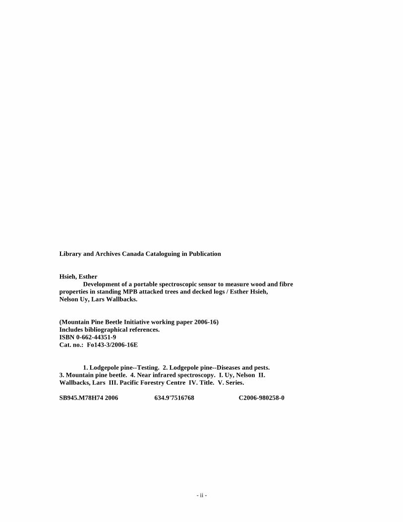
The LabSpec Pro vis-NIR spectrometer, manufactured by Analytical Spectral Devices, (ASD) was used to collect all spectral data, both in the field and in the laboratory. The LabSpec Pro is a laboratory spectrometer that is comprised of three detectors which enable spectra between 350-2500 nm to be collected, and can also be field-portable with the custom designed backpack as shown in Figure 1. The LabSpec Pro can operate on a fully charged battery for 3 – 4 hours. A fibre optic cable connects the probe head to the spectrometer (Figure 1). This cable needs to be handled with care in the field, since excessive bending or impact will result in damaged fibres, compromising signal quality.

- 2 -

Figure 1. The LabSpec Pro is a laboratory spectrometer that can be made field portable with the custom backpack. There is a suite of probe heads available with the LabSpec Pro for various applications. For this project four different probe heads were used to develop three models:

1) Wood Core Model - Straight Probe. The straight probe (Figure 2) has a 3 mm aperture, which created a 5 mm diameter measuring spot size when a 1 mm spacer was included to ensure a consistent measuring distance.

- 3 -

Figure 2. Straight probe used to develop wood core model in the laboratory.

2) In-Tree Model - Insertion Probes. Two probes were designed for in-tree measurement since this was a new application, and none of the stock probes were suitable. The challenge in the design of an insertion probe is the necessity to bend the light 90° within the diameter of a 12 mm bored hole. The first probe design (based on the original concept of Dr. Bob Meglen) used a 45° mirror imbedded in a prism to transmit and reflect the light 90° to the fibre bundles (Figure 3). The disadvantage with this design was there was a loss in signal throughput as well as a sinusoidal interference in the spectra collected which was associated with the added optical surfaces and complicated light path. The second probe design eliminated the use of additional optics by physically bending the fibre optic bundles through the length of the probe head (Figure 4). The signal throughput for this probe was much greater than the right angle reflectance probe and the sinusoidal noise was eliminated. However, in order to obtain the necessary curvature within the probe head, smaller fibres (100 �m diameter) were used. The smaller fibres do not have the cladding that the 200 �m diameter fibres have (used in the other probes). This resulted in lower signal transmission in the longer wavelengths causing a decrease in the signal to noise ratio starting at 1800 nm and sharply decreasing beyond 2200 nm. Similar to the straight probe, both insertion probes had apertures of 3 mm which created a 5 mm diameter measuring spot size when a 1 mm spacer was included to ensure a consistent measuring distance. Both the right angle reflectance and the bent optical fibre probes were field tested to determine which was the most suitable for in-tree field measurements.

- 4 -

Figure 3. Right angle reflectance designed insertion probe.

Figure 4. Insertion probe designed with internally bent fibre bundles.

3) Decked Logs Model – Contact Probe. The contact probe (Figure 5) had a measuring spot size diameter of 1.8 cm, and utilized a recessed window, so that a spacer to maintain a consistent measuring distance was not required. The optics of the contact probe differed from the straight and insertion probes because the fibre optic cable that collects the reflected light was mounted 45° to the illumination source. Since the probes used for wood core and in-tree measurements were constrained by the 12 mm core diameter, the fibre optic cable was used to transmit light from the source as well as collect the reflected light by dividing the fibre bundles, a design which is susceptible to specular reflection. A 45° offset in the light source and fibre optic cable used for collecting light reflected from the sample reduces the effect of specular reflection. This improved the signal quality of data collected using the contact probe.

- 5 -

Figure 5. Contact probe used to develop the model for decked logs.

2.2 Field Sampling

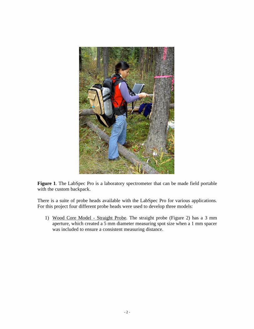
Field sampling was carried out in conjunction with MPBI Project # 8.15, and full details of site selection can be found in the final report (Trent et al. 2006). In summary, 36 mountain pine beetle-attacked sites were identified throughout the interior of BC based on representation of the various biogeoclimatic environments of lodgepole pine tree stands. A map of the selected sites is shown in Figure 6. Initial sampling for MPBI Project # 8.15 was conducted in 2004 and wood cores were collected from 360 trees (10 trees were sampled per site). From these 360 trees, a biogeoclimatically representative subset was selected for this project and used to develop an initial wood core model in the laboratory. This model was then used to predict moisture, basic density, blue stain and decay in the remaining 291 cores. From this data, a group of trees were identified which represented the full range of all four variables. These trees were targeted for the field trials and comprised the sample set for the final models.

- 6 -

Figure 6. A map of central British Columbia showing sample site locations for Trent et al. (2006), biogeoclimatic sub zones and major geographic features.

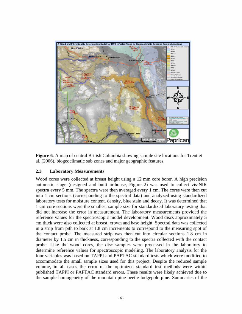
2.3 Laboratory Measurements

Wood cores were collected at breast height using a 12 mm core borer. A high precision automatic stage (designed and built in-house, Figure 2) was used to collect vis-NIR spectra every 5 mm. The spectra were then averaged every 1 cm. The cores were then cut into 1 cm sections (corresponding to the spectral data) and analyzed using standardized laboratory tests for moisture content, density, blue stain and decay. It was determined that 1 cm core sections were the smallest sample size for standardized laboratory testing that did not increase the error in measurement. The laboratory measurements provided the reference values for the spectroscopic model development. Wood discs approximately 5 cm thick were also collected at breast, crown and base height. Spectral data was collected in a strip from pith to bark at 1.8 cm increments to correspond to the measuring spot of the contact probe. The measured strip was then cut into circular sections 1.8 cm in diameter by 1.5 cm in thickness, corresponding to the spectra collected with the contact probe. Like the wood cores, the disc samples were processed in the laboratory to determine reference values for spectroscopic modeling. The laboratory analysis for the four variables was based on TAPPI and PAPTAC standard tests which were modified to accommodate the small sample sizes used for this project. Despite the reduced sample volume, in all cases the error of the optimized standard test methods were within published TAPPI or PAPTAC standard errors. These results were likely achieved due to the sample homogeneity of the mountain pine beetle lodgepole pine. Summaries of the

- 7 -

reference methods based on TAPPI and PAPTAC standards are given below, and further details are given in the appendix. Moisture Content – based on TAPPI T-258, PAPTAC G.3 test methods This method determines moisture content for wood samples on a wet weight basis. The average wet weight for the 1 cm core sections was 0.3g and 1.6g for the 1.8 cm disc sections. After the samples were oven dried, the weight loss was used to calculate the original moisture content using the following formula:

% Moisture = (wet weight – dry weight)*100/wet weight Density – based on TAPPI T-258, PAPTAC A.8P test methods The basic density for each wood sample was calculated using the following formula: Basic Density = dry weight/green volume The samples were soaked overnight and then water displacement was used to determine the green volume. The samples were then oven dried overnight to obtain the dry weight. Blue Stain – based on TAPPI T-527, PAPTAC E.5 test methods The industry standardized testing for colour measurement uses the CIE L*a*b* coordinates which is a colour system described by three axes, L* a* and b*, that uniquely define any colour. L* is a measure of lightness, a* measures colour differences from red to green and b* measures colour differences from yellow to blue. The Technobrite colourimeter was used to measure blue stain on the wood samples using D-b*. Delta b* (D-b*) is a measure of the difference between the b* of a sample and a reference. The wood samples were ground using a mini-Wiley mill with a 40 mesh screen to obtain a more homogenous measuring surface. A custom made sample holder was constructed from black Nylatron plastic with a 2.7 cm diameter and 2 mm depth to accommodate the reduced sample size. A sample of ground unstained mountain pine beetle-attacked sound wood was used as a reference and five scans were averaged for each measurement. Decay – based on TAPPI T-212, PAPTAC G.6 and G.7 test methods Solubility of wood in 1% NaOH is an indicator of decay. Approximately 0.25g of each sample (ground using a 40 mesh screen) was cooked in 12.5 ml of 1% NaOH for 1 hour. The NaOH soluble wood was separated from the insoluble wood using 103 grade Millipore filter paper. The insoluble wood was oven dried overnight and the weight loss was used to calculate the percentage of 1% caustic solubility using the following formula: 1% Caustic Soluble Wood = (Total dry sample weight) – (Insoluble sample weight)*100/Dry sample weight

- 8 -

The remaining portion of the sample was used to determine the moisture content of the sample, which was usually between 8%-10% since the samples had been oven dried and stored in the laboratory. The moisture content was used to determine the initial dry sample weight.

2.4 Calibrations

For the wood cores, spectra were collected every 5 mm along the length of the core using a high precision automated stage, and averaged every 1 cm. For the in-tree measurements, spectra were collected every 5 mm using the manually operated insertion probe and averaged every 1 cm. The spectra were averaged every 1 cm since it was determined to be the minimum sample volume required for laboratory processing without increasing the error. For the discs, spectra were collected and samples were processed every 1.8 cm since this was the measuring spot size of the contact probe. All calibrations were developed using chemometrics, a form of statistical analysis which utilizes computer-based mathematical techniques. It is a powerful method for identifying correlations in spectra and physical variables. All models were generated using Unscrambler chemometric software to calculate multi-variate partial least squared (PLS 2) calibrations to simultaneously predict moisture, density, blue stain and decay. For each spectrum, sixty co-adds were collected. No pre-processing was performed on the spectra and all spectra were autoscaled (1/stdev). All calibrations were generated using cross validation. All calibration models were validated using independent samples not included in the calibration sample sets.

3 Results and Discussion

Three PLS models were developed to measure moisture, density, blue stain and decay for three different applications: 1) wood cores 2) standing trees 3) decked logs. 3.1 Model Developed on Wood Cores with Straight Probe

The final model for wood cores was developed simultaneously with the in-tree model (which will be discussed in the next section). Spectra were collected in the laboratory on the wood cores that were extracted for the in-tree measurements during the field trial, before they were processed using laboratory methods to obtain reference values. It was expected that a model developed in the laboratory would have smaller errors than a field model since environmental variability in temperature, humidity and ambient light is reduced. By developing a model using spectra collected in the field simultaneously with a model developed using spectra collected in the laboratory for the same samples, the effect of external environmental variables can be directly measured.

- 9 -

A 12 component PLS2 model was generated. Thirty-seven 12 mm cores were used to calibrate the model and 11 cores were used for validation. Each core was divided into 1 cm sections for a total of 450 samples. The length of the cores (from pith to bark) ranged from 3 to 21 cm, and each data point represents a 1 cm section of the core. The results are shown below. Table 1. Summary of the results from the PLS2 model generated for measuring wood cores.

R

(Cal)

SEC R

(Val)

SEP Error in Reference

Method

Moisture 0.95 1.4% 0.93 1.7% 1.3% (Marrs)

Basic Density 0.57 42 kg/m3 0.21 45 kg/m3 5.6 kg/m3 (TAPPI)

Blue Stain (D-b*) 0.80 2.5 0.85 2.4 0.6 (TAPPI)

Decay (1% Caustic

Solubility)

0.87 2.4 % 0.83 2.6% 2.0% (CPPA)

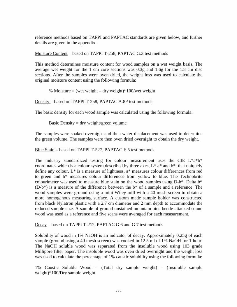
Moisture The model predicts moisture with high accuracy (Figure 7) and has a strong correlation with respect to the TAPPI (oven dried) method. The published error in the TAPPI reference method is 1.3% while the standard error in prediction (SEP) of the spectroscopic model is 1.7%, which indicates that the model is only contributing a 0.4% error. This result was achieved largely because the absorption peaks of the water molecules in the NIR region are readily identified by the model and confirms that NIR spectroscopy is an effective tool for measuring wood moisture.

- 10 -

Wood Core Moisture Using Vis-NIR

Calibration Validation

Figure 7. Calibration and validation model results for moisture measurement on wood cores in the laboratory using a straight probe. From the moisture profiles of the 11 cores used for validation (Figure 8), it can be clearly seen that the model predicts trends in the moisture data with high accuracy. Furthermore, we can see from these profiles that the moisture content is near or below the fibre saturation point and, in general, decreases from pith to bark. This trend has been the general observation throughout the entire 100 mountain pine beetle-killed trees used in this study and is contrary to what is normally observed in live or green trees where water transportation occurs in sap wood. This can have important implications for the forest products industry utilizing stands from these sites. Pulp mills for example, can anticipate that chips (especially purchased chips which will be comprised of sapwood) sourced from mountain pine beetle-killed trees will generally be near or below the fibre saturation point, and can optimize their operation accordingly.

- 11 -

10

15

20

25

30

35

% M

ois

ture

11 Cores (Pith to Bark, 1cm increments)

Lab Moist

Vis-NIR Moist

1

2

3 4

56

78

9

10

11

Figure 8. Moisture profiles for 11 cores comparing lab reference values (TAPPI) and vis-NIR measurements (both plotted on the y-axis). Note that each core (plotted on the x-axis) is a different length. Density Of the four properties, density is the most challenging to model because there are multiple chemical constituents with absorption peaks in the vis-NIR region that affect density. NIR density models have a published SEP of ~ 40 kg/m3 (Jones et al.) which is relatively large compared to the reported TAPPI error (5.6 kg/m3) for measuring basic density. The model had a SEP for measuring density in wood cores of 45 kg/m3 (similar to published results). While this is a relatively large error compared with the laboratory standard test, to determine how well the model would perform for a larger density range, two very high density cores sections (comprised of knots) were added to the original validation set. It is not reasonable to expect the model to accurately predict outside of the range it has been calibrated for, or to accurately predict samples not represented in the calibration set i.e., knots versus sound wood. However, since the model was able to identify the two knot samples as higher density samples (Figure 10), this demonstrates that the model is able to show density trends. While a vis-NIR model does not measure density as accurately as the TAPPI lab method it can be a very useful way for determining density trends rapidly, and in non-laboratory environments. For example, this density model will be able to distinguish relative density differences between stands of trees, which can be valuable for field crews determining wood material strategies. One of the biggest challenges with showing a strong correlation between lab (TAPPI) measured density and vis-NIR predicted density is that the total density variation (~100 kg/m3) for all the mountain pine beetle samples is small compared to the measurement error (45 kg/m3). To capture a larger density range on wood core measurements for lodgepole pine trees, earlywood and latewood need to be separated. In practice this will be difficult to achieve because growth rings are separated by millimetres in lodgepole

- 12 -

pine, whereas the spectrometer spot size is 5 mm. Regardless, the best indicator of model accuracy is the SEP, as it is independent of the range of variation.

Wood Core Density Using Vis-NIR

Calibration Validation

Figure 9. Calibration and validation model results for measuring density on wood cores in the laboratory using a straight probe.

- 13 -

Wood Core Density Using Vis-NIR

Predictions

Figure 10. Predictions including knot samples for measuring density on wood cores in the laboratory using a straight probe. As can be seen from the density profiles from the 11 validation cores (Figure 11), even though the density predictions are conservative, the model does trend the data.

0.3

0.4

0.5

0.6

0.7

0.8

0.9

Density (

kg/m

3)

11 Cores (Pith to Bark, 1cm increments)

Lab Density

Vis-NIR Density

1

2 3

4

5

6

78

910

11

Figure 11. Density profiles for 11 cores comparing lab reference values (TAPPI) and vis-NIR measurements (both plotted on the y-axis). Note that each core (plotted on the x-axis) is a different length. Blue Stain

- 14 -

Similar to moisture, blue stain is absorbed in a small spectral region, so it was expected that vis-NIR spectroscopy would model blue stain well. Furthermore, the Technobrite analyzer which is used to make the reference measurements is also based on light reflection, as is the vis-NIR spectrometer, so it was also expected that the two methods would show a strong correlation. The delta b* (D-b*) measurement from the CIE L*a*b* coordinate system was used to determine blue stain values used to develop the spectroscopic model. The SEP for blue stain was 2.4, compared to the TAPPI error for the D-b* which is 0.6. It should be understood that the TAPPI error is for colour measurement on paper and paperboard, which are materials with surfaces much more homogeneous than milled wood. Surface roughness and inhomogeneity scatter reflected light which adversely affects spectroscopic measurements. Therefore, it is unlikely that a model based on milled wood will ever achieve an error as low as a method based on paper or paperboard. Also, it should be noted that the D-b* measurements were collected on a smaller sample size than the TAPPI standard, and therefore there may be an offset in the values in the D-b* reported for this project with respect to measurements taken using the standard sample size.

Wood Core Blue Stain Using Vis-NIR

Calibration Validation

Figure 12. Calibration and validation model results for measuring blue stain on wood cores in the laboratory using a straight probe. From the profiles (Figure 13) not only can it be seen that the model predicts blue stain with good accuracy, but it is also exceptional at differentiating blue stained wood (below ~ 5 D-b*) from sound wood (above ~ 5 D-b*) as is shown by the sudden drop off along the profiles.

- 15 -

-5

0

5

10

15

20

Blu

e S

tain

(D

-b*)

11 Cores (Pith to Bark, 1cm increments)

Lab D-b*

Vis-NIR D-b*

1

2

3

4

56

7

8

910

11

Figure 13. Blue stain profiles for 11 cores comparing lab reference values (TAPPI) and the vis-NIR measurements (both plotted on the y-axis). Note that each core (plotted on the x-axis) is a different length. Decay Similar to density, decay is more challenging to model than moisture or blue stain because there are multiple regions in the spectrum that contribute to identifying the constituents of decay. However the model was better able to elucidate relevant spectral regions for decay than for density. The model SEP for the decay was 2.6%, which when compared to the TAPPI error of 2.0% indicates that the spectroscopic model only contributes a 0.6% error. A modified version of this model was also used to predict decay values for 291 cores used in Trent et al., 2006). Decay prediction were made for cores at 1 cm increments and then averaged to give a decay value for the tree and site. By using the model to predict decay, an estimated 15 days of laboratory analysis was saved for the MPBI 8.15 project.

- 16 -

Wood Core Decay Using Vis-NIR

Calibration Validation

Figure 14. Calibration and validation results for measuring decay on wood cores in the laboratory using a straight probe.

5

10

15

20

25

30

35

40

Decay (

1%

Caustic S

olu

bility)

11 Cores (Pith to Bark, 1cm increments)

Lab Caust Sol

Vis-NIR Caust Sol

1

2

34

5

6

78

9 10

11

Figure 15. Decay profiles for 11 cores comparing lab reference values (TAPPI) and vis-NIR measurements (both plotted on the y-axis). Note that each core (plotted on the x-axis) is a different length.

- 17 -

3.2 Field Model Developed on Standing Trees with Right Angle Reflectance

Probe

A model using the spectra collected in the field with the right angle reflectance probe was developed concurrently with the laboratory model developed on wood cores. The field spectra were collected from pre-selected biogeoclimatic sites throughout the interior of BC. Core borers 12 mm in diameter were used to extract cores at breast height. The pith to bark length was measured to determine the insertion depth of the probe. The right angle reflectance probe was inserted into the bored tree hole so that it was aligned with the pith. In-tree spectra were collected from pith to bark every 5 mm, and then averaged every 1 cm. The cores were bagged, sealed, chilled and brought back to the lab for wet chemistry analysis. A second field trial using the same methodology as the first trial was conducted with the internally bent fibre bundles insertion probe. Similar to the first field trial, a wood core model and in-tree model were developed simultaneously. The results showed that the right angle reflectance probe produced superior models in both cases for moisture, density and decay. Predictions for blue stain (which is measured using visible light) were similar for the models developed with both probes. This indicates the information in the longer wavelengths (1800-2300 nm) is important to developing a model for moisture, density and decay. The spectrometer hardware manufacturer (ASD) recommended future developmental work be focused on increasing the fibre size in the internally bent fibre optic probe. Improving the signal quality in the longer wavelengths in the internally bent fibre probe will likely be technically easier to achieve, more economical and show better results than trying to improve the optical configuration/materials of the right angle reflectance probe. The results for the in-tree model developed with the right angle reflectance insertion probe are shown in Table 2. A 15 component PLS2 model was generated. Twenty-seven 12 mm cores were used to calibrate the model and nine cores were used for validation. Each core was divided into 1 cm sections for a total of 275 samples. The length of the cores (from pith to bark) ranged from 3 cm to 21 cm, and each data point represents a 1 cm section of the core. Table 2. Summary of the results from the field model developed on standing trees with the right angle reflectance insertion probe.

R

(Cal)

SEC R

(Val)

SEP Error in Ref

Method

Moisture 0.94 1.3% 0.67 2.7% 1.3% (Marrs)

Basic Density 0.56 40 kg/m3 0.14 49 kg/m3 5.6 kg/m3 (Tappi)

Blue Stain (D-b*) 0.90 1.6 0.79 2.7 0.3 (Technodyne)

Decay (1% Caustic

Solubility)

0.81 1.6% 0.65 3.5% 2.0% (CPPA)

As mentioned in the previous section, it was expected that the in-tree model would be less accurate and have lower correlation with reference values than the model developed

- 18 -

in the controlled laboratory environment. The spectral data were collected over 8 days in the field and were subjected to temperature differences between days and trees which can cause an energy shift in the absorption peaks. During conditions of high humidity the water had a tendency to condense on to the probe tip, which affected the quality of the spectral data and added artefacts. Also, ensuring that the in-tree spectral measurements were aligned with the correct section of the extracted wood core used for the laboratory analysis was more challenging than in the lab. Aligning the data for the laboratory model was straightforward, where both the spectral measurement and wet chemistry were done on the core. For the field measurements, the spectra were collected in the bored hole in the trees, while the wet chemistry was done on the extracted cores. Although care was taken to determine the correct insertion depth of the probe, the imperfect outer surface of the tree added a potential alignment error. The enclosed bore-hole environment of the in-tree measurement may have also contributed to the spectral variability because of the increased surface area and exposure to more complex light paths. Another challenge in the development of the in-tree model was the quality of the spectral data due to the sinusoidal noise interference associated with the right angle reflectance tip. Not only is it undesirable to have artefacts in the spectral data, another problem was that the sinusoidal interference varied from spectrum to spectrum. This is a challenge for chemometric analysis because it forces the model to account for spectral changes that aren’t related to the physical data, resulting in models that are less precise. Table 3 shows a comparison of the wood core and in-tree models. Table 3. A comparison of the predictions errors for the model developed on standing trees with the right angle reflectance probe and the model developed in the lab with the straight probe.

In-Tree SEP Lab SEP

Moisture 2.7% 1.7%

Basic Density 49 kg/m3 45 kg/m3

Blue Stain (D-b*) 2.7 2.4

Decay (1% Caustic Solubility) 3.5 % 2.6%

One of the observations that can be made about the in-tree model is that it is comprised of 15 principal components, in contrast to the 12 components for the wood core model. To understand the role of principal components (PC’s) in chemometric modeling, consider a system where there are only four independent variables, then it would only take four principle components in the model to completely describe the variation in the system. However, since our four variables of interest are embedded in a wood matrix, there are many more variables contained in the system. So the fact that the in-tree field model requires 15 components to describe the data compared to the 12 components required by the model developed on wood cores in the lab, indicates that the latter is a less complicated system. This corroborates our earlier hypothesis that an in-tree model will have to account for more variation than one developed in a lab. However, it is likely that the reduced number of PC’s, the stronger correlations and the smaller prediction errors of

- 19 -

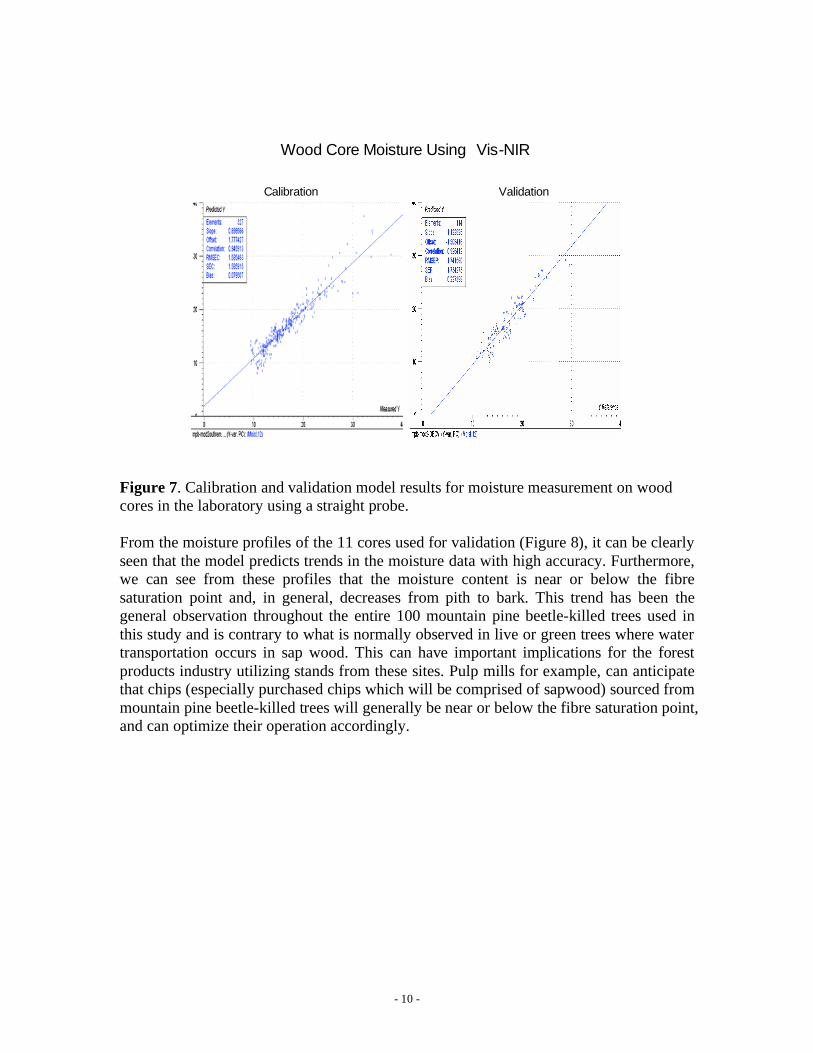
the wood core model can also be attributed to the improved quality of the spectral data collected with the straight probe. The following four sets of graphs are the results for the in-tree model developed using the right angle reflectance insertion probe. Moisture From the validation results, it can be seen that the model can predict moisture in standing trees and clearly trends moisture values. The SEP for the in-tree model increased to 2.7%, compared to 1.7% for the wood core model. Although this is a 1% increase in accuracy error, a moisture measurement with 2.7% accuracy for trees with a moisture range of 10% - 30% provides valuable information.

In-Tree Moisture Using Vis-NIR

Calibration Validation

Figure 16. Calibration and validation model results for measuring moisture in standing mountain pine beetle-attacked lodgepole pine trees using a right angle reflectance insertion probe.

Density In the model developed on standing trees, the error in the validation samples, SEP = 49 kg/m3, was only slightly higher than the density error for the wood core model (SEP = 45 kg/m3) and similar to published results for NIR density models. However, the correlation with the TAPPI measured density remains weak because the SEP is relatively large compared with the total density variation (~100 kg/m3) in the wood samples. As was done with the wood core model, to determine how well the model would perform for a larger density range, two very high density cores sections (comprised of knots) were added to the original validation set. It is not reasonable to expect the model to accurately

- 20 -

predict outside of the range it has been calibrated for or to accurately predict samples not represented in the calibration set i.e., knots versus sound wood. For the wood core model, higher density samples could be trended (Figures 10 and 11). However, when the high density samples were added to the in-tree validation set, the in-tree model wasn’t able to trend the higher density values but rather predicted them with a negative correlation. This indicates that the in-tree density model is not as robust as the one for wood cores, which is likely a result of the degraded quality of the spectral data collected with the right angle reflectance probe versus the straight probe.

In-Tree Density Using Vis-NIR

Calibration Validation

Figure 17. Calibration and validation model results for measuring density in standing mountain pine beetle-attacked lodgepole pine trees using a right angle insertion probe. Blue Stain The D-b* blue stain measurement was the variable least affected by the changes from the wood core model to the in-tree field model. The SEP for the in-tree model for blue stain increased to 2.7, compared to 2.4 for the wood core model. This indicates that the visible spectral region that is required to describe blue stain remains relatively stable when exposed to external field variables and is not greatly affected by the degraded quality of the spectral data of the right angle reflectance probe.

- 21 -

In-Tree Blue Stain (D -b*) Using Vis-NIR

Calibration Validation

Figure 18. Calibration and validation results for measuring blue stain in standing mountain pine beetle-attacked lodgepole pine trees using a right angle reflectance insertion probe. Decay The SEP for the in-tree model for decay increased to 3.5% compared to 2.6% for the wood core model. Despite the 0.9% decrease in accuracy, the in-tree model decay predictions still have accuracy only 1.5% lower than the laboratory caustic solubility standard test. For lodgepole pine, samples with caustic solubility lower than 20% are considered sound wood, 20% - 30% are decayed wood, and above 30% are advanced decay wood. The samples used in this project had decay values that ranged from sound wood to advanced decayed wood. A measurement with 3.5% accuracy is valuable in identifying differences in the extent of decay in standing trees. It should be noted that since the caustic solubility test was done on a reduced sample size to the recommended TAPPI method, the absolute values of the decay data reported for this project may include a small offset.

- 22 -

In-Tree Decay Using Vis-NIR

Calibration Validation

Figure 19. Calibration and validation results for measuring decay in standing mountain pine beetle-attacked lodgepole pine trees using a right angle reflectance probe. 3.3 Model developed for Decked Logs using Contact Probe

The last model developed was for decked logs and was completed by collecting spectra from discs in the laboratory. The contact probe (1.8 cm aperture) was used for this application. Initially, there was concern about the quality of the decked log model because the spectra would have to be collected parallel to the fibre direction. With the in-tree and wood core models, the spectra were collected perpendicular to the fibre direction to maximize the direct reflection of light. Since the radial surface (perpendicular to fibre direction) is not exposed in decked logs, the spectra had to be collected on the cross sectional plane (parallel to the fibre direction) where there was direct exposure to lumen cavities. The lumen cavities decrease the amount of light directly reflected back which reduces the signal quality. While this was a disadvantage to modeling on decked logs, a big advantage was the increased sample size. There was a 320% increase in measuring spot size between the 1 cm core sections and the 1.8 cm disc sections. An 11 component PLS2 model was generated. Nineteen discs were used to calibrate the model and seven discs were used for validation. Each disc was divided along a pith to bark strip into 1.8 cm sections for a total of 201 samples. The radius of the discs (from pith to bark) ranged from 6 cm to 16 cm, and each data point represents a 1.8 cm circular section of the disc.

- 23 -

Table 4. Summary of the results from the lab model developed for decked logs using a contact probe.

R

(Cal)

SEC R

(Val)

SEP Error in Ref

Method

Moisture 0.92 1.9% 0.94 1.3% 1.3% (Marrs)

Basic Density 0.53 35 kg/m3 0.63 31 kg/m3 5.6 kg/m3 (TAPPI)

Blue Stain (D-b*) 0.95 1.3 0.93 1.4 0.6 (TAPPI)

Decay (1% Caustic

Solubility)

0.9 2.1% 0.88 2.6% 2.0% (CPPA)

Table 5. A comparison of the predictions errors for all three models: 1) standing trees using the right angle reflectance tip; 2) wood cores using the straight probe; 3) decked logs using the contact probe.

In-Tree

SEP

Wood Core

SEP

Decked Log

SEP

Moisture 2.7% 1.7% 1.3%

Basic Density 49 kg/m3 45 kg/m3 31 kg/m3

Blue Stain (D-b*) 2.7 2.4 1.4

Decay (1% Caustic Solubility) 3.5 % 2.6% 2.6%

As can be seen in Table 5, the decked log model developed with the contact probe gave the best results. This indicates that the larger measuring spot and sample size obtained using the contact probe plays an important role in developing an accurate model. Moisture The model SEP for moisture is 1.3%, which is the same error as the oven dry reference method. This indicates that the spectroscopic error contribution to the model is negligible and the only way to improve this model would be to improve the reference method. As was observed in the wood core samples, the moisture content for the mountain pine beetle-attacked discs is below or near the fibre saturation point, confirming the observation that mountain pine beetle-killed trees rapidly loose the free water in their sapwood.

- 24 -

Decked Log Moisture Using Vis-NIR

Calibration Validation

Figure 20. Calibration and validation model results for measuring moisture in mountain pine beetle discs using a contact probe. Density The results using the contact probe for density were also significantly improved. The model SEP was 31 kg/m3, which not only is an improvement over the wood core and in-tree models, but it is also better than published data for NIR density models. Again, this is a strong indicator that the increased measuring spot of the contact probe and sample size play an important role in model accuracy. While the decked log model error is still significantly larger than the lab measurement, it is still a valuable tool for measuring density trends within a stand of trees or for applications that require rapid density assessments.

- 25 -

Decked Log Density Using Vis-NIR

Calibration Validation

Figure 21. Calibration and validation model results for measuring density in mountain pine beetle discs using a contact probe. Blue Stain The decked log model SEP for blue stain (1.4) also showed a significant improvement over the wood core and in-tree model (2.4, 2.7 respectively). As mentioned previously, it is unlikely that the error will be reduced to the 0.6 of the TAPPI reference method since milled wood measurements on the Technobrite colourimeter will always have a larger error than paper or paperboard.

- 26 -

Decked Log Blue Stain Using Vis-NIR

Calibration Validation

Figure 22. Calibration and validation model results for measuring blue stain in mountain pine beetle discs using a contact probe. Decay Decay was the only variable that did not show a significant improvement in predictions for the decked log model, but rather the SEP remained the same as the wood core model (2.6%). This may be explained by the increase in the signal to noise ratio in the longer wavelengths in all the probes, which plays an important role in modeling decay. It appears that the model predictions for decay may have reached their maximum performance with the spectral region provided and the probes currently available.

- 27 -

Decked Log Decay Using Vis-NIR

Calibration Validation

Figure 23. Calibration and validation results for measuring decay in mountain pine beetle discs using a contact probe. An additional model was created for decked logs using the contact probe, including green lodgepole pine samples not yet attacked by mountain pine beetles. Although this was not one of the goals of this project, the samples were available and it was of interest to compare the differences between a model developed with mountain pine beetle samples and one that also included green samples. As can be seen from the results presented in Table 6, the only variable that was really affected was the moisture (SEP increased to 3.6% from 1.3%). Otherwise the mountain pine beetle model behaved similarly to the model that also incorporated green lodgepole pine samples. The increase in error for moisture is likely a result of the peak shift in bound versus unbound water. As was mentioned earlier, the majority of the mountain pine beetle trees sampled in this project have moisture content below the fibre saturation point (unbound water), whereas green samples will have moisture content well above the fibre saturation point (bound water).

- 28 -

Table 6. Summary of the results from the lab model developed for decked logs with a contact probe including green lodgepole pine samples.

R

(Cal)

SEC R

(Val)

SEP Error in Ref

Method

Moisture 0.94 2.8% 0.91 3.1% 1.3% (Marrs)

Basic Density 0.69 29 kg/m3 0.55 35 kg/m3 5.6 kg/m3 (TAPPI)

Blue Stain (D-b*) 0.95 1.3 0.91 1.5 0.6 (TAPPI)

Decay (1% Caustic

Solubility)

0.89 2.0% 0.89 2.5% 2.0% (CPPA)

Decked Log Moisture Using Vis-NIR

(Including Green Samples)

Calibration Validation

Figure 24. Calibration and validation results for measuring moisture in mountain pine beetle and green lodgepole pine discs.

Although the disc model that includes green samples has a decrease in moisture accuracy (3.1%) compared to the disc model that only contains mountain pine beetle-attacked samples (1.3%), the error is still relatively small considering the moisture spans a range of 10% - 55%. If high accuracy moisture measurements are required, one way to improve the model would be to make separate calibrations for bound and unbound water. Note that the models for the decked logs were developed and validated in the laboratory. Field validation has yet to be done, and an offset adjustment may be required to accommodate environmental variability.

- 29 -

4 Conclusions

A portable spectroscopic sensor to measure wood and fibre properties in standing mountain pine beetle-attacked trees and decked logs was developed. Three models were developed to simultaneously measure moisture, density, blue stain and decay for three different applications; 1) wood cores 2) standing trees 3) decked logs. Each of the three applications utilized a different probe head which had a large effect on the accuracy of the models. The contact probe used for the decked log model, which had the largest measuring spot size and a 45°optical offset, produced the best model, while the insertion probe, which had the most complicated optics produced the model with the largest errors. The results demonstrate that vis-NIR spectroscopy can be used to measure moisture, blue stain, and decay to high accuracy both in the field and laboratory. Density trends can also be measured using vis-NIR spectroscopy, but with less accuracy than standard laboratory methods. The results suggest that future development of these NIR technologies is warranted as the measurements can play a significant role in assisting with the optimal end-use allocation of mountain pine beetle-killed lodgepole pine. Developmental work to improve the signal quality of the insertion probe will provide the opportunity to achieve higher accuracy for in-tree measurement. A more robust design of the fibre optic cable will make the sensor more durable for field applications.

5 Acknowledgements

This project was funded by the Government of Canada through the Mountain Pine Beetle Initiative, a six-year, $40 million Program administered by Natural Resources Canada, Canadian Forest Service. Publication does not necessarily signify that the contents of this report reflect the views or policies of Natural Resources Canada – Canadian Forest Service. Representative field sampling design was coordinated by Tennessee Trent (PAPRICAN) with the help from a large number of people representing public and private organizations. Steve Taylor, Rene Alfaro and Elizabeth Campbell helped with understanding the beetle outbreak history of the Chilcotin Plateau and the studies carried out by the Canadian Forest Service there. John Degagne (British Columbia Ministry of Forests) provided materials and maps for the Vanderhoof forest district. Cathy Koot of the University of British Columbia Alex Fraser Research Forest provided access and maps. Tom Olafson of WestFraser, Fraser Lake division provided maps and logistical support. Mike Pelchat (British Columbia Ministry of Forests) provided maps of the Quesnel Forest District and Mark Todd of Canfor, Prince George provided maps of the Prince George district. The design and manufacturing of the two insertion probes was coordinated by Analytical Spectral Devices. Numerous people at PAPRICAN contributed to this research effort. Linda Ishkintana worked on the laboratory analysis and experimental design of the wet chemistry. Morgan

- 30 -

Zhang and Jacquie Boivin helped to collect laboratory spectra. Tennessee Trent and Maxwell McRae helped with the field trials. Dave Pouw and Peter Taylor designed and built the automatic stage and its software interface to measure wood cores.

6 Cited Literature

Marrs, G.R. 1978. Oven Dry Procedure Evaluation. Form 2980-0 12/73 Internal Technical Report, Weyerhaeuser Company, 3. Jones, P.D.; Schimleck, L.R.; Peter, G.F.; Daniels, R.F.; Clark A. 2005. Nondestructive estimation of Pinus taedaI L. wood properties for samples from a wide range of sites in Georgia. Canadian Journal of Forest Research 35: 85-92. Trent, T.; Lawrence, V.; Woo, K. 2006. A wood and fibre quality deterioration model formountain pine beetle-infested trees by biogeoclimatic subzone. Mountain Pine Beetle Initiative Working Paper 2006-10. Natural Resources Canada, Canadian Forest Service, Pacific Forestry Centre, Victoria, BC. Web site: mpb.cfs.nrcan.gc.ca/research/projects/completed_e.html accessed September 6, 2006. Thrower, J.S.; Willis, R.; de Jong, R.; Gilbert, D.; Robertson, H. 2005. Sample plan to measure tree characteristics related to the shelf life of mountain pine beetle killed lodgepole pine trees in British Columbia. Mountain Pine Beetle Initiative Working Paper 2005-1. Natural Resources Canada, Canadian Forest Service, Pacific Forestry Centre, Victoria, BC. Web site: mpb.cfs.nrcan.gc.ca/research/projects/completed_e.html accessed September 6, 2006.

- 31 -

7 Appendix

One of the many challenges of this project was obtaining model accuracy with small samples sizes. The cores were cut into 1 cm sections using a razor blade resulting in a sample size 12 mm in diameter x 1 cm thick. The discs were cut into sections 1.8 cm in diameter x 1.5 cm thick. Reference data for developing the models were acquired using TAPPI and PAPTAC standards test standards modified for reduced sample size. Moisture Content Method – based on TAPPI T-258, PAPTAC G.3 test methods After the samples were cut, they were brushed to remove any dust/dirt or loose particles. The samples were weighed using a closed chamber balance to four decimal places. Samples were then oven dried overnight at 105°C. After drying, the samples were placed in a desiccator for 10 minutes before the dry weight was measured. The moisture content was determined by formula [1]. [1] % Moisture = Wet Weight (g) – Dry Weight (g) x 100 Wet Weight (g) Density Method – based on TAPPI T-258, PAPTAC A.8P test methods Basic density is measured by taking the ratio of the dry sample weight and green volume described in formula [2]. [2] Density = Dry weight (g) . Green volume (cm3) The dry weight was acquired during moisture determination. The green volume was obtained using water displacement method. The sample was fully immersed in DI water and soaked overnight. Then the sample was blotted softly in paper towel to remove surface water. A miniature water displacement apparatus (Figure 1) in a closed chamber balance was used to obtain an accurate volume measurement.

- 32 -

Figure 1. Water displacement apparatus for measuring the volume of a small sample. The needle was inserted into the sample to a depth of 0.5 mm and the sample was submerged 1mm below the surface. The water temperature and weight of the displaced water were then recorded and the volume of the sample in cm3 was calculated using formula [3]. [3] Volume of sample (cm3) = Weight displaced water (g) Density of water (g/cm3)* * Water Density/Temperature table referenced from: Lange’s Handbook of Chemistry, John A. Dean, 14th Ed. Blue Stain Method – based on TAPPI T-527, PAPTAC E.5 test methods The samples were ground using a mini Wiley mill using a 40 mesh screen. A customized sample holder made from black Nylatron plastic with a diameter of 2.7 cm and depth of 2 mm was used to collect D-b* measurements using the Technobrite colourimeter. A reference sample comprised of unstained sound mountain pine beetle wood was scanned prior to scanning the sample. D-b* measurements were calculated as the difference between the b* of the sample and the reference. All measurements were averaged over 5 scans. 1% Caustic Solubility Method – based on TAPPI T-212, PAPTAC G.6 and G.7 test methods Approximately 0.25g of ground wood sample (40 mesh) was weighed using a closed chamber balance to four decimal places and transferred to a 250-ml Erlenmeyer flask. The remaining ground wood was also weighed and used to determine the moisture content, which was then used to calculate the dry weight of the sample, formula [4].

- 33 -

[4] Dry Sample Weight = Wet Sample Weight x (1 - (% moisture) ) 100

12.5 ml of 1% NaOH solution was added to the flask with 0.25g ground wood. The flask was placed in a water bath at 100°C for 1 hour, stirring the sample after 5, 10 and 25 minutes. After 1 hour, the flask was cooled to room temperature then filtered using Millipore vacuum filtration with 103 grade filter paper. The residue (insoluble wood) was dried overnight at 105°C. The dry weight of the residue (insoluble wood) was obtained and the 1% caustic solubility calculated using formula [5].

[5] 1% caustic solubility = (Dry Sample Weight (g) – Dry Residue Weight (g)) x 100 Dry Sample Weight (g)

Contact:

Esther Hsieh - Technical Specialist Pulp and Paper Research Institute of Canada – PAPRICAN 3800 Wesbrook Mall Vancouver, BC. V6S 2L9 ehsieh@paprican.ca 604 222-3200 ext. 347 604 222-3207 facsimile

This publication is funded by the Government of Canada through the Mountain Pine Beetle Initiative, a program administered by Natural Resources Canada, Canadian Forest Service (web site: mpb.cfs.nrcan.gc.ca).

Contact:For more information on the Canadian Forest Service, visit our web site at:www.nrcan.gc.ca/cfs-scf

or contact the Pacific Forestry Centre506 West Burnside RoadVictoria, BC V8Z 1M5Tel: (250) 363-0600 Fax: (250) 363-0775www.pfc.cfs.nrcan.gc.ca

To order publications on-line, visit the Canadian Forest Service Bookstore at:

bookstore.cfs.nrcan.gc.ca