Estimates for Singular Integral Operators

Computational Methods and Function TheoryVolume 8 (2008), No. 1, 35–46

Estimates for Singular Integral Operators

Peter C. Fenton and John Rossi

(Communicated by J. Milne Anderson and Philip J. Rippon)

To Walter Hayman, our friend and teacher

Abstract. Estimates are obtained for∫ ∞0

K(r, t)φ(t) dt, where K(r, t) mayhave a singularity at t = −r.

Keywords. Singular integral operator, subharmonic function.

2000 MSC. 47G10, 30D15.

1. Introduction

If u(z) is an entire subharmonic function of order less than 1 which is harmonicoff the negative real axis and such that u(0) = 0, then

u(z) =

∫ ∞

0

K0(z, t)μ∗(t)

dt

t,

where K0(z, t) = z/(z + t), and μ∗(t) is a non-decreasing function on [0,∞) thatvanishes in some right neighbourhood of 0. The integral, which (for some z) maybe −∞, is interpreted as a Cauchy principal value when z is real and negative.The infimum and supremum of u(z)

A(r) = A(r, u) = inf|z|=r

u(z) =

∫ ∞

0

K0(−r, t)μ∗(t)dt

t,(1)

B(r) = B(r, u) = sup|z|=r

u(z) =

∫ ∞

0

K0(r, t)μ∗(t)

dt

t,(2)

are connected in well-known ways. For example, if u(z) has order ρ minimaltype, where 0 < ρ < 1, then, on a sequence of r → ∞, A(r) > (cos πρ)B(r).Proofs of this result — the so-called cos πρ Theorem — abound. The authors

Received August 28, 2006, in revised form October 24, 2006.Published online March 27, 2007.

ISSN 1617-9447/$ 2.50 c© 2008 Heldermann Verlag

36 P. C. Fenton and J. Rossi CMFT

recently gave one [4]; (see also [5]) that uses a technique of Beurling [1, p. 4],[2, p. 34], the idea being to separately relate A(r) and B(r) to

(3) Φ(r) =

∫ r

0

φ(t) dt,

where φ(t) = μ∗(t)/t, and thereby to each other. The intention of this note isto apply Beurling’s technique to a class of integral operators in which the kernelK0(r, t) is replaced by something more general. This not only extends the rangeof Beurling’s technique but, in providing a setting in which the cosπρ Theoremappears as a particular case, allows another perspective on this fundamentalresult. The methods used here are implicit in [4].

2. Results

We are concerned with estimates for∫ ∞

0K(r, t)φ(t) dt, where K(r, t) and φ(t)

are such that

(i) K(r, t) is defined on D ≡ (−∞,∞)× [0,∞) \ {(−x, x) : x ≥ 0};(ii) limt→−r(r + t)K(r, t) exists, for all r < 0;(iii) Kt = ∂K/∂t exists on D;(iv) K(r, 0) = 1, and limt→∞ K(r, t) = 0, for all r �= 0;(v) φ(t) is a non-negative function on (0,∞), integrable on (0, t), for every

positive t, and such that∫ ∞

0φ(t) dt = ∞.

We suppose that there is a continuous, non-negative function n(t) on [0,∞), andthere are numbers λ and μ, such that, with N(r) =

∫ r

0n(t) dt, either

(4)

∫ ∞

0

K(r, t)n(t) dt = λN(r), for all r > 0,

or

(5)

∫ ∞

0

K(−r, t)n(t) dt = μN(r), for all r > 0.

We suppose also that, as t → ∞, N(t) → ∞ and, for all r, K(r, t)N(t) → 0.These conditions are satisfied with K(r, t) = K0(r, t), n(t) = σtσ−1, for anyfixed σ satisfying 0 < σ < 1, λ = πσ csc πσ and μ = πσ cot πσ.

Finally we suppose that, with Φ(t) given by (3),

(6)Φ(t)

N(t)→ 0 as t→∞.

We will prove the following result.

Theorem 1. Suppose that K(r, t), φ(t), Φ(t), n(t) and N(t) are as above. Thereis an unbounded set E = E(Φ, N) ⊂ (0,∞), and there are numbers br, withbr →∞ as r →∞, such that

8 (2008), No. 1 Estimates for Singular Integral Operators 37

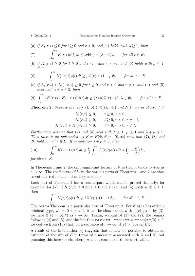
(a) if Kt(r, t) ≤ 0 for t ≥ 0 and r > 0, and (4) holds with λ ≥ 1, then

(7)

∫ ∞

0

K(r, t)φ(t) dt ≤ λΦ(r)− (λ− 1)br for all r ∈ E;

(b) if Kt(r, t) ≥ 0 for t ≥ 0 and r < 0 and r �= −t, and (5) holds with μ ≤ 1,then

(8)

∫ ∞

0

K(−r, t)φ(t) dt ≥ μΦ(r) + (1− μ)br for all r ∈ E;

(c) if Kt(r, t) + Kt(−r, t) ≥ 0 for t ≥ 0 and r > 0 and r �= t, and (4) and (5)hold with λ + μ ≤ 2, then

(9)

∫ ∞

0

(K(r, t)+K(−r, t)

)φ(t) dt ≥ (λ+μ)Φ(r)+(2−λ−μ)br for all r ∈ E.

Theorem 2. Suppose that K(r, t), φ(t), Φ(t), n(t) and N(t) are as above, that

Kt(r, t) ≤ 0, t ≥ 0, r > 0,

Kt(r, t) ≥ 0, t ≥ 0, r < 0, r �= −t,

Kt(r, t) + Kt(−r, t) ≥ 0, t ≥ 0, r > 0, r �= t.

Furthermore assume that (4) and (5) hold with λ ≥ 1, μ ≤ 1 and λ + μ ≤ 2.Then there is an unbounded set E = E(Φ, N) ⊂ (0,∞) such that (7), (8) and(9) hold for all r ∈ E. If in addition λ + μ ≥ 0, then

(10)

∫ ∞

0

K(−r, t)φ(t) dt ≥ μ

λ

∫ ∞

0

K(r, t)φ(t) dt +(1− μ

λ

)br,

for all r ∈ E.

In Theorems 1 and 2, the only significant feature of br is that it tends to +∞ asr →∞. The coefficients of br in the various parts of Theorems 1 and 2 are thusessentially redundant unless they are zero.

Each part of Theorem 1 has a counterpart which can be proved similarly; forexample, for (a): if Kt(r, t) ≥ 0 for t ≥ 0 and r > 0, and (4) holds with λ ≤ 1,then ∫ ∞

0

K(r, t)φ(t) dt ≥ λΦ(r) + (1− λ)br, for all r ∈ E.

The cos πρ Theorem is a particular case of Theorem 2. For if u(z) has order ρminimal type, where 0 < ρ < 1, it can be shown that, with Φ(r) given by (3),we have Φ(r) = O(rρ) as r → ∞. Taking account of (1) and (2), the remarkfollowing (4) and (5), and the fact that πσ csc πσ+πσ cot πσ = πσ cot(πσ/2) < 2,we deduce from (10) that, on a sequence of r →∞, A(r) > (cos πρ)B(r).

A result of the first author [6] suggests that it may be possible to obtain anestimate of the size of E in terms of a measure associated with Φ and N , butpursuing this here (or elsewhere) was not considered to be worthwhile.


3. Proof of Theorem 1

Beurling’s technique picks out the points rα defined by

(11) aα ≡ Φ(rα)− αN(rα) = max{Φ(t)− αN(t) : t ≥ 0}for any α > 0. Since Φ(t) and N(t) are continuous on [0,∞), and

Φ(t)− αN(t) → −∞ as t→∞,

from (6), rα exists (possibly not uniquely) for all α > 0. Moreover, since Φ(t) isunbounded above as t→∞, aα →∞, and thus rα →∞, as α → 0+. We define

(12) E = {rα : α > 0}.Notice that

(13) Φ′(rα) = αN ′(rα) for all α > 0.

For the left- and right-hand derivatives, Φ′−(t) and Φ′+(t), exist, and we haveΦ′−(t) ≤ Φ′+(t), for every t, since φ(t) is non-negative. On the other hand, fromthe definition of rα we get Φ′−(rα) ≥ αN ′(rα) ≥ Φ′+(rα), and N ′(rα) exists sincen(t) is continuous, by assumption. Thus Φ′−(rα) = Φ′+(rα), i.e. Φ′(rα) exists,and Φ′(rα) = αN ′(rα).

Concerning (a), define β(r) :=∫ ∞

0K(r, t)φ(t) dt, so that, on integrating by parts,

β(r) = −∫ ∞

0

Kt(r, t)Φ(t) dt ≤ −∫ ∞

0

Kt(r, t) (αN(t) + aα) dt(14)

=

∫ ∞

0

K(r, t)αn(t) dt + aα = λαN(r) + aα.

Here we have used (11), the fact that K(r, t)Φ(t) → 0 as t → ∞ (which followsfrom (6) and our assumption that K(r, t)N(t) → 0 as t→∞) and the first partof condition (iv). Taking r = rα and recalling that αN(rα) = Φ(rα) − aα, (14)yields β(rα) ≤ λΦ(rα) + (1− λ)aα, which is (7).

The proof of (8) is similar, except for the complication of a possible singularityin the kernel. Given r > 0 and ε > 0, we have, integrating by parts,

I1 :=

∫ ∞

r+ε

K(−r, t)φ(t) dt(15)

= −K(−r, r + ε)Φ(r + ε)−∫ ∞

r+ε

Kt(−r, t)Φ(t) dt

≥ −K(−r, r + ε)Φ(r + ε)−∫ ∞

r+ε

Kt(−r, t) (αN(t) + aα) dt

= −K(−r, r + ε) {Φ(r + ε)− αN(r + ε)− aα}+

∫ ∞

r+ε

K(−r, t)αn(t) dt.


When r = rα, the first term is, with c = limε→0 K(−r, r + ε) (which exists from(ii)),

(16) −(c + O(1))ε−1 {Φ(rα + ε)− Φ(rα)− α(N(rα + ε)−N(rα))} = O(1),

using (13). Similarly, when r = rα,

I2 :=

∫ r−ε

0

K(−r, t)φ(t) dt(17)

= K(−r, r − ε)Φ(r − ε)−∫ r−ε

0

Kt(−r, t)Φ(t) dt

≥ K(−r, r − ε)Φ(r + ε)−∫ r−ε

0

Kt(−r, t) (αN(t) + aα) dt

= K(−r, r − ε) {Φ(r − ε)− αN(r − ε)− aα}+

∫ r−ε

0

K(−r, t)αn(t) dt + aα

=

∫ r−ε

0

K(−r, t)αn(t) dt + aα + O(1).

Combining (15), (16) and (17), taking r = rα and allowing ε → 0+, we obtain∫ ∞

0

K(−rα, t)φ(t) dt ≥ μαN(rα) + aα = μΦ(rα) + aα(1− μ),

using (5), which gives (8).

For (c), we have, as in the proof of (b),

I1 =

∫ ∞

rα+ε

(K(r, t) + K(−r, t)) φ(t) dt

≥∫ ∞

rα+ε

(K(r, t) + K(−r, t)) αn(t) dt + O(1),

I2 =

∫ rα−ε

0

(K(r, t) + K(−r, t)) φ(t) dt

≥∫ rα−ε

0

(K(r, t) + K(−r, t)) αn(t) dt + 2aα + O(1),

as ε → 0+. Adding these inequalities, taking r = rα and allowing ε → 0+, weobtain ∫ ∞

0

(K(rα, t) + K(−rα, t)) φ(t) dt

≥ (λ + μ)αN(rα) + 2aα = (λ + μ)Φ(rα) + (2− λ− μ)aα,

which is (9).


4. Proof of Theorem 2

First, (7), (8) and (9) evidently hold on the same set E. Also, (10) is clear from(7) and (8) if μ ≥ 0 , while if μ < 0 we have, from (9) and (7),∫ ∞

0

(K(r, t) + K(−r, t)) φ(t) dt

≥(1 +

μ

λ

)λΦ(r) + (2− λ− μ)br

≥(1 +

μ

λ

) ∫ ∞

0

K(r, t)φ(t) dt +((

1 +μ

λ

)(λ− 1) + (2− λ− μ)

)br,

=(1 +

μ

λ

) ∫ ∞

0

K(r, t)φ(t) dt +(1 +

μ

λ

)br,

and (10) follows again.

5. An example

As was pointed out earlier, the cos πρ Theorem follows from Theorem 2 whenK(r, t) = K0(r, t). Are there significantly different kernels to which Theorem 2applies? We will show that the answer is yes, that

(18) K(r, t) =r

(1− θ)(r + t)

(1− 2θr2

r2 + (r + t)2

),

where θ is a constant such that 0 ≤ θ ≤ 1/4, satisfies the hypotheses of The-orem 2, with n(t) = σtσ−1, where 0 < σ < 1. Our estimates are rough andready and it will be clear that with more effort the range of allowed θ could beexpanded somewhat. K0(r, t) corresponds to θ = 0. Regrettably, we know of noprior function-theoretic context in which the kernels (18) play a part. They areintroduced here simply to ensure that the generality suggested by Theorem 2 isnot in fact bogus.

Evidently (i), (ii), (iii) and (iv) are satisfied, and

(19) Kt(r, t) = − r

(1− θ)(r + t)2

(1− 2θr2(r2 + 3(r + t)2)

(r2 + (r + t)2)2

).

Concerning the second term in the bracketed expression, note that if b ≥ a ≥ 0,a(a + 3b)/(a + b)2 = (a2 + 3ab)/(a2 + 2ab + b2) ≤ 1, while for b such that0 ≤ b ≤ a, a(a + 3b)/(a + b)2 has a maximum value of 9/8 when b = a/3. Sincewe are assuming that 0 ≤ θ ≤ 1/4, the bracketed expression is positive, and thusKt(r, t) ≤ 0 for t ≥ 0 and r > 0, and Kt(r, t) ≥ 0 for t ≥ 0 and r < 0 and r �= −t.To determine the sign of Kt(r, t) + Kt(−r, t) for t ≥ 0, note that it is sufficientto take r = 1. Now

(20) K(1, t) + K(−1, t) = H(1 + t) + H(1− t),


where

(21) H(x) =x2 + (1− 2θ)

(1− θ)(x3 + x).

Also

(22) H ′′(x) =2x6 + 6(1− 4θ)x4 + 6(1− 2θ)x2 + 2(1− 2θ)

(1− θ)(x(1 + x2))3,

so, since 0 ≤ θ ≤ 1/4, H(x) is convex for x > 0, and from this and (20),

Kt(1, t) + Kt(−1, t) = H ′(1 + t)−H ′(1− t) > 0,

for 0 ≤ t < 1. For t > 1, we rewrite (20) as

K(1, t) + K(−1, t) = H(t + 1)−H(t− 1),

so that

Kt(1, t) + Kt(−1, t) = H ′(t + 1)−H ′(t− 1) > 0.

Thus Kt(r, t) + Kt(−r, t) ≥ 0 for t ≥ 0 and r > 0 and r �= −t.

We take n(t) = σtσ−1, where σ satisfies 0 < σ < 1, so that N(t) = tσ. NowN(t) →∞ as t→∞ and, for all r, K(r, t)N(t) → 0 as t→∞. Also (4) and (5)hold with

λ =σ

1− θ

∫ ∞

0

tσ−1

1 + t

(1− 2θ

1 + (1 + t)2

)dt,(23)

μ =σ

1− θ

∫ ∞

0

tσ−1

1− t

(1− 2θ

1 + (1− t)2

)dt.(24)

Since

(25) L ≡∫ ∞

0

2tσ−1

(1 + t)(1 + (1 + t)2)dt ≤

∫ ∞

0

tσ−1

1 + tdt = π csc πσ,

we have λ ≥ πσ csc πσ > 1, and further, after a change of variable in the integralover the interval [1, 2],

M ≡∫ ∞

0

2tσ−1

(1− t)(1 + (1− t)2)dt(26)

=

∫ 1

0

2 (tσ−1 − (2− t)σ−1)

(1− t)(1 + (1− t)2)dt +

∫ ∞

2

2tσ−1

(1− t)(1 + (1− t)2)dt

≥∫ 1

0

tσ−1 − (2− t)σ−1

1− tdt +

∫ ∞

2

tσ−1

1− tdt

=

∫ ∞

0

tσ−1

1− tdt = π cot πσ,


so that μ ≤ πσ cot πσ < 1. It remains to show that λ + μ < 2, and to this endwe evaluate L and M , given by (25) and (26). For L, we integrate

zσ−1

(1 + z)(1 + (1 + z)2)

around the curve made up of a large circle centred at the origin, together withthe upper positive real axis and the lower positive real axis. The contributionof the circle is negligible. The upper axis contributes L/2 and the lower axis−e2πσiL/2, so that the entire integral is (1 − e2πσi)L/2. There are three poles,one at −1 with residue −eπσi, one at −1 + i with residue −2(σ−1)/2e3π(σ−1)i/4/2,and one at −1− i with residue −2(σ−1)/2e5π(σ−1)i/4/2, and the sum of the residuesis

eπσi

(−1 + 2(σ−1)/2 cos

π(σ − 1)

4

).

Equating the expressions for the integral and dividing by 2ieπσi, we obtain

(27) L = 2π

(1− 2(σ−1)/2 cos

π(σ − 1)

4

)csc πσ.

Similarly, by integratingzσ−1

(1− z)(1 + (1− z)2)

around the same curve, but with indentations into the upper and lower halfplanes at z = 1, we obtain

(28) M = 2π

(cos πσ + 2(σ−1)/2 cos

3π(σ − 1)

4

)csc πσ.

Since cos(3π(σ − 1)/4) − cos(π(σ − 1)/4) = −2 cos(πσ/2) sin(π(1 − σ)/4) and1 + cos πσ = 2 cos2(πσ/2), we obtain after simplification,

L + M = 2π

(cot

πσ

2− 2(σ−1)/2 csc

πσ

2sin

π(1− σ)

4

).

Thus, since∫ ∞

0tσ−1/(1 + t) dt = π csc πσ,

∫ ∞0

tσ−1/(1 − t) dt = π cot πσ, andcsc πσ + cot πσ = cot(πσ/2), we have

(29) λ + μ =1

1− θ

((1− 2θ)πσ cot

πσ

2+ 2θπσ2(σ−1)/2 csc

πσ

2sin

π(1− σ)

4

).

Now πσ cot(πσ/2) < 2, and we will therefore have λ + μ < 2 if it can be shownthat 2πσ2(σ−1)/2 csc(πσ/2) sin(π(1− σ)/4) < 2; that is, if F (σ)G(σ) < 1, where

(30) F (σ) = 2σ/2πσ

2csc

πσ

2and G(σ) = cos

πσ

4− sin

πσ

4.

Since F (σ) is increasing and G(σ) is decreasing, for 0 < σ ≤ 1, and sinceF (1)G(2/3) = 0.813 . . . , we conclude that F (σ)G(σ) < 1 on [2/3, 1]. In the sameway the inequality can be extended in turn to [1/2, 2/3], [1/3, 1/2], [1/4, 1/3],


[3/16, 1/4], [1/8, 3/16] and [1/16, 1/8]. It remains to show that F (σ)G(σ) < 1for 0 < σ < 1/16.

Now, 2σ/2 = eσ(log 2)/2, and, for t < 1,

et = 1 + t +t2

2

(1 +

t

3+ · · ·

)≤ 1 + t +

t2

2

1

1− t3

< 1 + t +3

4t2.

Thus, for 0 < σ < 1/16, we certainly have

(31) 2σ/2 < 1 +log 2

2σ + σ2.

Also, sin t ≥ t−t3/6, and, for 0 < t < 1/2, 1/(1−t) < 1+2t, so t csc t < 1+t2/3,and therefore, for 0 < σ < 1/16, it is clear that

(32)πσ

2csc

πσ

2< 1 + σ2.

Further, cos t− sin t ≤ 1− t + t3/6, and so, for 0 < σ < 1/16, we have

(33) cosπσ

4− sin

πσ

4< 1− π

4σ + σ2.

Combining (31), (32) and (33), we deduce that, if 0 < σ < 1/16,

F (σ)G(σ) <

(1 +

log 2

2σ + σ2

) (1 + σ2

) (1− π

4σ + σ2

)

= 1−(

π

4− log 2

2

)σ + Δ(σ),

where, loosely estimating higher terms (using the fact that (log 2)/2 < 1 andπ/4 < 1, and ignoring the minus sign),

(34) Δ(σ) ≤ 4σ2 + 4σ3 + 4σ4 + 2σ5 + σ6,

Since Δ(σ) ≤ 6σ2 for 0 < σ < 1/4, and since 6σ < π/4 − (log 2)/2 for0 < σ < 1/16, we obtain

F (σ)G(σ) < 1− σ

(π

4− log 2

2− 6σ

)< 1,

for 0 < σ < 1/16.

Thus λ+μ ≤ 2, and the hypotheses of the second part of Theorem 2 are satisfied.We deduce that∫ ∞

0

K(−r, t)φ(t) dt >μ

λ

∫ ∞

0

K(r, t)φ(t) dt + br,

for all r in an unbounded set E, where

λ =1

1− θ(πσ csc πσ − θσL) , μ =

1

1− θ(πσ cot πσ − θσM) ,

and L and M are given by (27) and (28).


6. Concluding remarks

If, instead of (4) in the first part of part (a) of Theorem 1, we assume that∫ ∞

0

K(r, t)n(t) dt = (λ + O(1))N(r) as r →∞,

and also that λ > 1, then, as can be easily checked, we obtain the weakerconclusion ∫ ∞

0

K(r, t)φ(t) dt ≤ (λ + O(1))Φ(r) as r →∞through E. The rest of Theorem 1 can be modified in a similar way.

As an application, consider

K(r, t) =1− e−r

et − e−r,

which satisfies conditions (i)–(iv). We have

Kt(r, t) = −et(1− e−r)

(et − e−r)2,

so that Kt(r, t) ≥ 0, for t ≥ 0 and r < 0 and r �= −t. Also, given a constant σ,with 0 < σ < 1, we have, for r > 0,∫ ∞

0

K(−r, t)eσt dt = eσr

(∫ ∞

−∞

eσt

1− etdt + O(1)

).

Since ∫ ∞

−∞

eσt

1− etdt =

∫ 0

−∞

eσt

1− etdt +

∫ ∞

0

eσt

1− etdt

=

∫ ∞

0

e−σt

1− e−tdt−

∫ ∞

0

e−(1−σ)t

1− e−tdt

=∞∑

j=0

∫ ∞

0

e−(j+σ)t − e−(j+1−σ)t dt

=∞∑

j=0

(1

j + σ− 1

j + 1− σ

),

we have ∫ ∞

0

K(−r, t)n(t) dt = (μ + O(1))N(r),

with n(t) = eσt, N(t) = σ−1(eσt − 1) and

μ = σ

∞∑j=0

(1

j + σ− 1

j + 1− σ

)= 1− σ

(1

1− σ−

∞∑j=1

(1

j + σ− 1

j + 1− σ

)).


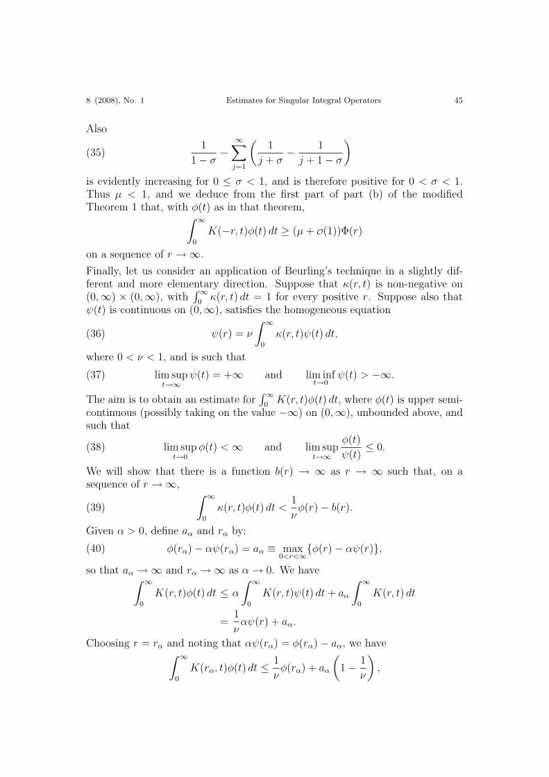
Also

1

1− σ−

∞∑j=1

(1

j + σ− 1

j + 1− σ

)(35)

is evidently increasing for 0 ≤ σ < 1, and is therefore positive for 0 < σ < 1.Thus μ < 1, and we deduce from the first part of part (b) of the modifiedTheorem 1 that, with φ(t) as in that theorem,∫ ∞

0

K(−r, t)φ(t) dt ≥ (μ + O(1))Φ(r)

on a sequence of r →∞.

Finally, let us consider an application of Beurling’s technique in a slightly dif-ferent and more elementary direction. Suppose that κ(r, t) is non-negative on(0,∞) × (0,∞), with

∫ ∞0

κ(r, t) dt = 1 for every positive r. Suppose also thatψ(t) is continuous on (0,∞), satisfies the homogeneous equation

(36) ψ(r) = ν

∫ ∞

0

κ(r, t)ψ(t) dt,

where 0 < ν < 1, and is such that

(37) lim supt→∞

ψ(t) = +∞ and lim inft→0

ψ(t) > −∞.

The aim is to obtain an estimate for∫ ∞

0K(r, t)φ(t) dt, where φ(t) is upper semi-

continuous (possibly taking on the value −∞) on (0,∞), unbounded above, andsuch that

(38) lim supt→0

φ(t) <∞ and lim supt→∞

φ(t)

ψ(t)≤ 0.

We will show that there is a function b(r) → ∞ as r → ∞ such that, on asequence of r →∞,

(39)

∫ ∞

0

κ(r, t)φ(t) dt <1

νφ(r)− b(r).

Given α > 0, define aα and rα by:

(40) φ(rα)− αψ(rα) = aα ≡ max0<r<∞

{φ(r)− αψ(r)},so that aα →∞ and rα →∞ as α → 0. We have∫ ∞

0

K(r, t)φ(t) dt ≤ α

∫ ∞

0

K(r, t)ψ(t) dt + aα

∫ ∞

0

K(r, t) dt

=1

ναψ(r) + aα.

Choosing r = rα and noting that αψ(rα) = φ(rα)− aα, we have∫ ∞

0

K(rα, t)φ(t) dt ≤ 1

νφ(rα) + aα

(1− 1

ν

),


and (39) follows.

The inequality (39) affords us another proof of the cosπρ Theorem. Indeed by aresult of Kjellberg [7] (see also [3, pp. 232–235])

(41) 2B(r) ≤∫ ∞

0

κ(r, t)φ(t) dt,

whereφ(t) = A(t) + B(t)

and

κ(r, t) =4

π2t

rtlog r

t

( rt)2 − 1

.

Then from the discussion following equation (1.12) in [3],∫ ∞

0κ(r, t) dt = 1 and

equation (36) holds with ν = 2/(1 + cos πρ) and ψ(t) = tρ. (Since B(r) isunbounded it is clear from (41) that φ is unbounded.) Assume that B(r) = O(rρ).Using (41) and (39) we obtain on a sequence r that

A(r) ≥ cos πρB(r) + b(r).

References

1. R. P. Boas, Entire Functions, Academic Press, 1954.2. M. L. Cartwright, Integral Functions, Cambridge University Press, 1956.3. D. Drasin and D. Shea, Convolution inequalities, regular variation and exceptional sets, J.

Analyse Math. 29 (1976), 232–293.4. P. C. Fenton and J. Rossi, Phragmen-Lindelof theorems, Proc. Amer. Math. Soc. 132 (2004),

761–768.5. , cos πρ theorems for δ-subharmonic functions, J. Analyse Math. 92 (2004), 385–396.6. P. C. Fenton, Density in cos πρ theorems for δ-subharmonic functions, to appear in Analysis

26 (2006).7. B. Kjellberg, A theorem on the minimum modulus of entire functions, Math. Scand. 12

(1963), 5–11.

Peter C. Fenton E-mail: [email protected]: University of Otago, Department of Mathematics and Statistics, Dunedin, NewZealand.

John Rossi E-mail: [email protected]: Virginia Tech, Department of Mathematics, Blacksburg, VA 24061-0123, U.S.A.

Documents

Estimates for Singular Integral Operators