ESTIMATES OF OPTIMAL BACKWARD PERTURBATIONS FOR

ESTIMATES OF OPTIMAL BACKWARD PERTURBATIONSFOR LINEAR LEAST SQUARES PROBLEMS∗

JOSEPH F. GRCAR† , MICHAEL A. SAUNDERS‡ , AND ZHENG SU§

Abstract. Numerical tests are used to validate a practical estimate for the optimal backwarderrors of linear least squares problems. This solves a thirty-year-old problem suggested by Stewartand Wilkinson.

Key words. linear least squares, backward errors, optimal backward error

AMS subject classifications. 65F20, 65F50, 65G99

“A great deal of thought, both by myself and by J. H. Wilkinson, hasnot solved this problem, and I therefore pass it on to you: find easilycomputable statistics that are both necessary and sufficient for thestability of a least squares solution.” — G. W. Stewart [24, pp. 6–7]

1. Introduction. Our aim is to examine the usefulness of a certain quantity asa practical backward error estimator for the least squares (LS) problem:

minx‖Ax− b‖2 where b ∈ Rm and A ∈ Rm×n.

Throughout the paper, x denotes an arbitrary vector in Rn. If any such x solvesthe LS problem for data A+ δA, then the perturbation δA is called a backward errorfor x. This name is borrowed from the context of Stewart and Wilkinson’s remarks,backward rounding error analysis, which finds and bounds some δA when x is acomputed solution. When x is arbitrary, it may be more appropriate to call δA a“data perturbation” or a “backward perturbation” rather than a “backward error.”All three names have been used in the literature.

The size of the smallest backward error is µ(x) = minδA ‖δA‖F . A precise defini-tion and more descriptive notation for this are

µ(x) =

{the size of data perturbation, for matrices in least squaresproblems, that is optimally small in the Frobenius norm,as a function of the approximate solution x

}= µ(LS)

F (x) .

This level of detail is needed here only twice, so we usually abbreviate it to “optimalbackward error” and write µ(x). The concept of optimal backward error originatedwith Oettli and Prager [19] in the context of linear equations.

If µ(x) can be estimated or evaluated inexpensively, then the literature describesthree uses for it.

1. Accuracy criterion. When the data of a problem have been given with an errorthat is greater than µ(x), then x must be regarded as solving the problem,to the extent the problem is known. Conversely, if µ(x) is greater than the

∗Version 13 of July 12, 2007. Technical Report SOL 2007-1.†Center for Computational Sciences and Engineering, Lawrence Berkeley National Lab, Berkeley,

CA 94720-8142 ([email protected]). The work of this author was supported by the U.S. Departmentof Energy under contract no. DE-AC02-05-CH11231.‡Department of Management Science and Engineering, Stanford University, Stanford, CA 94305-

4026 ([email protected]). The research of this author was supported by National Science Foun-dation grant CCR-0306662 and Office of Naval Research grant N00014-02-1-0076.§Department of Applied Mathematics and Statistics, SUNY Stony Brook, Stony Brook, NY 11733

([email protected]).

1

2 JOSEPH GRCAR, MICHAEL SAUNDERS, AND ZHENG SU

uncertainty in the data, then x must be rejected. These ideas originatedwith John von Neumann and Herman Goldstine [18] and were rediscoveredby Oettli and Prager.

2. Run-time stability estimation. A calculation that produces x with small µ(x)is called backwardly stable. Stewart and Wilkinson [24, pp. 6–7], Karlsonand Walden [15, p. 862] and Malyshev and Sadkane [16, p. 740] emphasizedthe need for “practical” and “accurate and fast” ways to determine µ(x) forleast squares problems.

3. Exploring the stability of new algorithms. Many fast algorithms have beendeveloped for LS problems with various kinds of structure. Gu [12, p. 365][13] explained that it is useful to examine the stability of such algorithmswithout having to perform backward error analyses of them.

When x is a computed solution, Wilkinson would have described these uses for µ(x)as “a posteriori” rounding error analyses.

The exact value of µ(x) was discovered by Walden, Karlson and Sun [27] in 1995.To evaluate it, they recommended a formula that Higham had derived from theirpre-publication manuscript [27, p. 275] [14, p. 393],

µ(x) = min

{‖r‖‖x‖

, σmin[A B]

}, B =

‖r‖‖x‖

(I − rrt

‖r‖2

), (1.1)

where r = b − Ax is the residual for the approximate solution, σmin is the smallestsingular value of the m×(n+m) matrix in brackets, and ‖·‖ means the 2-norm unlessotherwise specified. There are similar formulas when both A and b are perturbable,but they are not discussed here. It is interesting to note that a prominent part ofthese formulas is the optimal backward error of the linear equations Ax = b, namely

η(x) ≡ ‖r‖‖x‖

= µ(LE)

F (x) = µ(LE)

2 (x) . (1.2)

The singular value in (1.1) is expensive to calculate by dense matrix methods, soother ways to obtain the backward error have been sought. Malyshev and Sadkane[16] proposed an iterative process based on the Golub-Kahan process [8] (often calledLanczos bidiagonalization).

Other authors including Walden, Karlson and Sun have derived explicit approx-imations for µ(x). One estimate in particular has been studied in various forms byKarlson and Walden [15], Gu [12], and Grcar [11]. It can be written as

µ(x) =∥∥(‖x‖2AtA+ ‖r‖2I

)−1/2Atr∥∥ =

∥∥(AtA+ η2I)−1/2

Atr∥∥ /‖x‖ . (1.3)

For this quantity:• Karlson and Walden showed [15, p. 864, eqn. 2.5 with y = yopt] that, in the

notation of this paper,

2

2 +√

2µ(x) ≤ f(yopt) ,

where f(yopt) is a complicated expression that is a lower bound for the small-est backward error in the spectral norm, µ(LS)

2 (x). It is also a lower boundfor µ(x) = µ(LS)

F (x) because ‖δA‖2 ≤ ‖δA‖F. Therefore Karlson and Walden’sinequality can be rearranged to

µ(x)

µ(x)≤ 2 +

√2

2≈ 1.707 . (1.4)

OPTIMAL BACKWARD PERTURBATIONS FOR LEAST SQUARES 3

• Gu [12, p. 367, cor. 2.2] established the bounds

‖r∗‖‖r‖

≤ µ(x)

µ(x)≤√

5 + 1

2≈ 1.618 , (1.5)

where r∗ is the unique, true residual of the LS problem. He used theseinequalities to prove a theorem about the definition of numerical stability forLS problems. Gu derived the bounds assuming that A has full column rank.The lower bound in (1.5) should be slightly less than 1 because it is alwaystrue that ‖r∗‖ ≤ ‖r‖, and because r ≈ r∗ when x is a good approximation toa solution.

• Finally, Grcar [11, thm. 4.4], based on [10], proved that µ(x) asymptoticallyequals µ(x) in the sense that

limx→ x∗

µ(x)

µ(x)= 1 , (1.6)

where x∗ is any solution of the LS problem. The hypotheses for this are thatA, r∗, and x∗ are not zero. This limit and both equations (1.1) and (1.3) donot restrict the rank of A or the relative sizes of m and n.

All these bounds and limits suggest that (1.3) is a robust estimate for the optimalbackward error of least squares problems. However, this formula has not been exam-ined numerically. It receives only brief mention in the papers of Karlson and Walden,and Gu, and neither they nor Grcar performed numerical experiments with it. Theaim of this paper is to determine whether µ(x) is an acceptable estimate for µ(x) inpractice, thereby answering Stewart and Wilkinson’s question.

2. When both A and b are perturbed. A practical estimate for the optimalbackward error when both A and b are perturbed is also of interest. In this case, theoptimal backward error is defined as

min∆A,∆b

{‖∆A, θ∆b‖F : ‖(A+ ∆A)y − (b+ ∆b)‖2 = min},

where θ is a weighting parameter. (Taking the limit θ →∞ forces ∆b = 0, giving thecase where only A is perturbed.) From Walden et al. [27] and Higham [14, p. 393] theexact backward error is

µA,b(x) = min{√νη, σmin[A B]},

where

η =‖r‖‖x‖

, B =√νη

(I − rrt

‖r‖2

), ν =

θ2‖x‖2

1 + θ2‖x‖2.

Thus, µA,b(x) is the same as µ(x) in (1.1) with η changed to η ≡√νη (as noted by

Su [25]). Hence we can estimate µA,b(x) using methods for estimating µ(x), replacingη = ‖r‖/‖x‖ by η =

√ν‖r‖/‖x‖. In particular, from (1.3) we see that µA,b(x) may

be estimated by

µA,b(x) =∥∥(AtA+ η2I

)−1/2Atr∥∥ /‖x‖ . (2.1)

The asymptotic property (1.6) also follows because µ(x) and µA,b(x) have the sameessential structure.

In the remainder of the paper, we consider methods for computing µ(x) whenonly A is perturbed, but the same methods apply to computing µA,b(x).


3. The KW problem and projections. Karlson and Walden [15, p. 864] drawattention to the full-rank LS problem

K =

[A‖r‖‖x‖I

], v =

[r

0

], min

y‖Ky − v‖, (3.1)

which proves central to the computation of µ(x). It should be mentioned that LSproblems with this structure are called “damped”, and have been studied in thecontext of Tikhonov regularization of ill-posed LS problems [3, pp. 101–102]. Weneed to study three such systems involving various A and r. To do so, we need somestandard results on QR factorization and projections. We state these in terms of afull-rank LS problem miny ‖Ky − v‖ with general K and v.

Lemma 3.1. Suppose the matrix K has full column rank and QR factorization

K = Q

[R

0

]= Y R , Q =

[Y Z

], (3.2)

where R is upper triangular and nonsingular, and Q is square and orthogonal, so thatY tY = I, ZtZ = I, and Y Y t +ZZt = I. The associated projection operators may bewritten as

P = K(KtK)−1Kt = Y Y t, I − P = ZZt. (3.3)

Lemma 3.2. For the quantities in Lemma 3.1, the LS problem miny ‖Ky − v‖has a unique solution and residual vector defined by Ry = Y tb and t = v −Ky, andthe two projections of v satisfy

Pv = Ky = Y Y tv, ‖Ky‖ = ‖Y tv‖, (3.4)

(I − P )v = t = ZZtv, ‖t‖ = ‖Ztv‖. (3.5)

(We do not need (3.5), but it is included for completeness.)

We now find that µ(x) in (1.3) is the norm of a certain vector’s projection. LetK and v be as in the KW problem (3.1). From (1.3) and the definition of P in (3.3)we see that ‖x‖2 µ(x)2 = vtPv, and from (3.4) we have vtPv = ‖Y tv‖2. It followsagain from (3.4) that

µ(x) =‖Pv‖‖x‖

=‖Y tv‖‖x‖

=‖Ky‖‖x‖

, (3.6)

where Y and ‖Y tv‖ may be obtained from the reduced QR factorization K = Y Rin (3.2). (It is not essential to keep the Z part of Q.) Alternatively, ‖Ky‖ may beobtained after the KW problem is solved by any method.

4. Evaluating the estimate. Several ways to solve minx ‖Ax − b‖2 producematrix factorizations that can be used to evaluate µ(x) in (1.3) or (3.6) efficiently.We describe some of these methods here. If x is arbitrary, then the same proceduresmay still be used to evaluate µ(x) at the extra cost of calculating the factorizationsjust for this purpose.


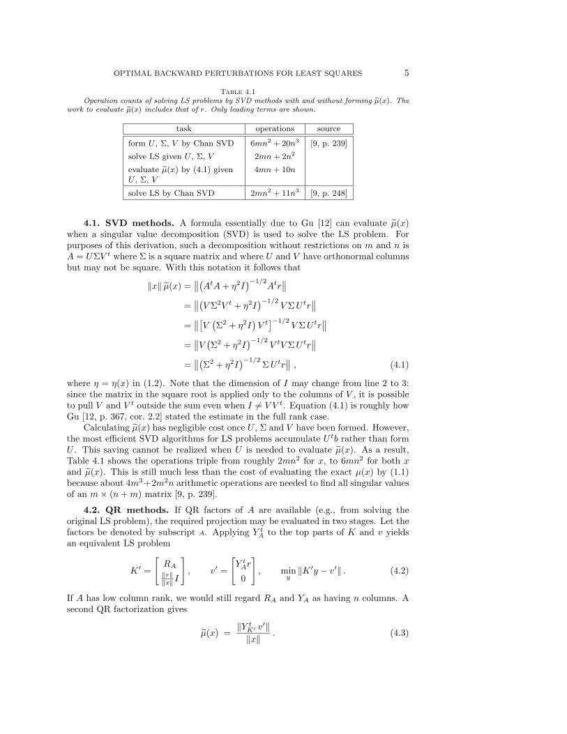
Table 4.1Operation counts of solving LS problems by SVD methods with and without forming µ(x). The

work to evaluate µ(x) includes that of r. Only leading terms are shown.

task operations source

form U , Σ, V by Chan SVD 6mn2 + 20n3 [9, p. 239]

solve LS given U , Σ, V 2mn+ 2n2

evaluate µ(x) by (4.1) givenU , Σ, V

4mn+ 10n

solve LS by Chan SVD 2mn2 + 11n3 [9, p. 248]

4.1. SVD methods. A formula essentially due to Gu [12] can evaluate µ(x)when a singular value decomposition (SVD) is used to solve the LS problem. Forpurposes of this derivation, such a decomposition without restrictions on m and n isA = UΣV t where Σ is a square matrix and where U and V have orthonormal columnsbut may not be square. With this notation it follows that

‖x‖ µ(x) =∥∥(AtA+ η2I

)−1/2Atr∥∥

=∥∥(V Σ2V t + η2I

)−1/2V ΣU tr

∥∥=∥∥[V (Σ2 + η2I

)V t]−1/2

V ΣU tr∥∥

=∥∥V (Σ2 + η2I

)−1/2V tV ΣU tr

∥∥=∥∥(Σ2 + η2I

)−1/2ΣU tr

∥∥ , (4.1)

where η = η(x) in (1.2). Note that the dimension of I may change from line 2 to 3:since the matrix in the square root is applied only to the columns of V , it is possibleto pull V and V t outside the sum even when I 6= V V t. Equation (4.1) is roughly howGu [12, p. 367, cor. 2.2] stated the estimate in the full rank case.

Calculating µ(x) has negligible cost once U , Σ and V have been formed. However,the most efficient SVD algorithms for LS problems accumulate U tb rather than formU . This saving cannot be realized when U is needed to evaluate µ(x). As a result,Table 4.1 shows the operations triple from roughly 2mn2 for x, to 6mn2 for both xand µ(x). This is still much less than the cost of evaluating the exact µ(x) by (1.1)because about 4m3 +2m2n arithmetic operations are needed to find all singular valuesof an m× (n+m) matrix [9, p. 239].

4.2. QR methods. If QR factors of A are available (e.g., from solving theoriginal LS problem), the required projection may be evaluated in two stages. Let thefactors be denoted by subscript A. Applying Y tA to the top parts of K and v yieldsan equivalent LS problem

K ′ =

[RA‖r‖‖x‖I

], v′ =

[Y tAr

0

], min

y‖K ′y − v′‖ . (4.2)

If A has low column rank, we would still regard RA and YA as having n columns. Asecond QR factorization gives

µ(x) =‖Y tK′ v′‖‖x‖

. (4.3)


Table 4.2Operation counts of solving LS problems by QR methods and then evaluating µ(x) when m ≥ n.

The work to evaluate Y tAr includes that of r. Only leading terms are shown.

task operations source

solve LS by Householder QR, retaining YA 2mn2 [9, p. 248]

form Y tAr and v′ 4mn

apply Y tK′ to v′ 8

3n3 [15, p. 864]

finish evaluating µ(x) by (4.3) 2n

Table 4.3Summary of operation counts to solve LS problems, to evaluate the estimate µ(x), and to

evaluate the exact µ(x). Only leading terms are considered.

task operations m = 1000, n = 100 source

solve LS by QR 2mn2 20,000,000 Table 4.2

solve LS by QR andevaluate µ(x) by (4.3)

2mn2 + 83n3 22,666,667 Table 4.2

solve LS by Chan SVD 2mn2 + 11n3 31,000,000 Table 4.1

solve LS by Chan SVD andevaluate µ(x) by (4.3)

2mn2 + 413n3 33,666,667 Tables 4.1, 4.2

solve LS by Chan SVD andevaluate µ(x) by (4.1)

6mn2 + 20n3 80,000,000 Table 4.1

evaluate µ(x) by (1.1) 4m3 + 2m2n 4,200,000,000 [9, p. 239]

This formula could use two reduced QR factorizations. Of course, YK′ needn’t bestored because Y tK′ v

′ can be accumulated as K ′ is reduced to triangular form.Table 4.2 shows that the optimal backward error can be estimated at little addi-

tional cost over that of solving the LS problem when m � n. Since K ′ is a 2n × nmatrix, its QR factorization needs only O(n3) operations compared to O(mn2) for thefactorization of A. Karlson and Walden [15, p. 864] considered this same calculationin the course of evaluating a different estimate for the optimal backward error. Theynoted that sweeps of plane rotations most economically eliminate the lower block ofK ′ while retaining the triangular structure of RA.

4.3. Operation counts for dense matrix methods. Table 4.3 summarizesthe operation counts of solving the LS problem and estimating its optimal backwarderrors by the QR and SVD solution methods for dense matrices. It is clear thatevaluating the estimate is negligible compared to evaluating the true optimal backwarderror. Obtaining the estimate is even negligible compared to solving the LS problemby QR methods.

The table shows that the QR approach also gives the most effective way to eval-uate µ(x) when the LS problem is solved by SVD methods. Chan’s algorithm forcalculating the SVD begins by performing a QR factorization. Saving this intermedi-ate factorization allows (4.3) to evaluate the estimate with the same, small marginalcost as in the purely QR case of Table 4.3.

4.4. Sparse QR methods. Equation (4.3) uses both factors of A’s QR decom-position: YA to transform r, and RA occurs in K ′. Although progress has been made


towards computing both QR factors of a sparse matrix, notably by Adlers [1], it isconsiderably easier to work with just the triangular factor, as described by Matstoms[17]. Therefore methods to evaluate µ(x) are needed that do not presume YA.

The simplest approach may be to evaluate (3.6) directly by transforming K toupper triangular form. Notice that AtA and KtK have identical sparsity patterns.Thus the same elimination analysis would serve to determine the sparse storage spacefor both RA and R. Also, Y tv can be obtained from QR factors of

[K v

]. The

following Matlab code is often effective for computing µ(x) for a sparse matrix Aand a dense vector b:

[m,n] = size(A); r = b - A*x;

normx = norm(x); eta = norm(r)/normx;

p = colamd(A);

K = [A(:,p); eta*speye(n)];

v = [ r ; zeros(n,1)];

[c,R] = qr(K,v,0); muKW = norm(c)/normx;

Note that colamd returns a good permutation p without forming A’*A, and qr(K,v,0)

computes the required projection c = Y tv without storing any Q.

4.5. Iterative methods. If A is too large to permit the use of direct methods,we may consider iterative solution of the original problem min ‖Ax− b‖ as well as theKW problem (3.1):

miny‖Ky − v‖ ≡ min

y

∥∥∥∥[ AηI

]y −

[r0

]∥∥∥∥ , η ≡ η(x) =‖r‖‖x‖

. (4.4)

In particular, LSQR [20, 21, 23] takes advantage of the damped least squares structurein (4.4). Using results from Saunders [22], we show here that the required projectionnorm is available within LSQR at negligible additional cost.

For problem (4.4), LSQR uses the Golub-Kahan bidiagonalization of A to formmatrices Uk and Vk with theoretically orthonormal columns and a lower bidiagonalmatrix Bk at each step k. With β1 = ‖r‖, a damped LS subproblem is defined andtransformed by a QR factorization:

minwk

∥∥∥∥[ BkηI]wk −

[β1e1

0

]∥∥∥∥ , Qk

[Bk β1e1

ηI 0

]=

Rk zkζk+1

qk

. (4.5)

The kth estimate of y is defined to be yk = Vkwk = (VkR−1k )zk. From [22, pp. 99–100],

the kth estimate of the required projection is given by

Ky ≈ Kyk ≡[AηI

]yk =

[Uk+1

Vk

]Qtk

[zk0

]. (4.6)

Orthogonality (and exact arithmetic) gives ‖Kyk‖ = ‖zk‖. Thus if LSQR terminatesat iteration k, ‖zk‖ may be taken as the final estimate of ‖Ky‖ for use in (3.6), givingµ(x) ≈ ‖zk‖/‖x‖. Since zk differs from zk−1 only in its last element, only k operationsare needed to accumulate ‖zk‖2.

LSQR already forms monotonic estimates of ‖y‖ and ‖v − Ky‖ for use in itsstopping rules, and the estimates are returned as output parameters. We see thatthe estimate ‖zk‖ ≈ ‖Ky‖ is another useful output. Experience shows that theestimates of such norms retain excellent accuracy even though LSQR does not usereorthogonalization.


Table 5.1Matrices used in the numerical tests.

matrix rows m columns n κ2(A)

(a) illc1033 1033 320 1.9e+4(b) well1033 1033 320 1.7e+2(c) prolate 100 ≤ m ≤ 1000 n < m up to 9.2e+10

5. Numerical tests with direct methods. This section presents numericaltests of the optimal backward error estimate. For this purpose it is most desirableto make many tests with problems that occur in practice. Since large collections oftest problems are not available for least squares, it is necessary to compromise byusing many randomly generated vectors, b, with a few matrices, A, that are relatedto real-world problems.

5.1. Description of the test problems. The first two matrices in Table 5.1,well1033 and illc1033, originated in the least-squares analysis of gravity-meterobservations. They are available from the Harwell-Boeing sparse matrix collection[7] and the Matrix Market [4]. The prolate matrices [26] are very ill-conditionedToeplitz matrices of a kind that occur in signal processing. As generated here theirentries are parameterized by a number a:

Ai,j =

2a if i = j,

sin(2aπ|i− j|)π|i− j| if i 6= j.

Since these matrices may be given any dimensions, a random collection is uniformlygenerated with 100 ≤ m ≤ 1000, 1 ≤ n < m, and − 1

4 ≤ a ≤14 .

Without loss of generality the vectors b in the LS problems may be restrictedto norm 1. Sampling them uniformly from the unit sphere poses a subtle problembecause, if A has more rows than columns, most vectors on the unit sphere are nearlyorthogonal to range(A). (To see this in 3-space, suppose that range(A) is the earth’saxis. The area below 45◦ latitude is much larger than the surface area in higherlatitudes. This effect is more pronounced for higher dimensional spheres.) Since leastsquares problems are only interesting when b has some approximation in terms of A’scolumns, b is sampled so that ∠(b, range(A)) is uniformly distributed, as follows:

b = c1PAu

‖PAu‖+ c2

(I − PA)u

‖(I − PA)u‖.

In this formula, (c1, c2) = (cos(θ), sin(θ)) is uniformly chosen on the unit sphere,PA : Rm → range(A) is the orthogonal projection, and u is uniformly chosen on theunit sphere in Rm using the method of Calafiore, Dabbene, and Tempo [5].

5.2. Description of the calculations. For the factorization methods, 1000sample problems are considered for each type of matrix in Table 5.1. For each sampleproblem, the solution x and the backward error estimate µ(x) are computed usingIEEE single precision arithmetic. The estimates are compared with the optimal back-ward error µ(x) from Higham’s equation (1.1) evaluated in double precision. Matrixdecompositions are calculated and manipulated using the LINPACK [6] subroutinessqrdc, sqrsl, and ssvdc, and for the higher precision calculations dqrdc, dqrsl, anddsvdc.


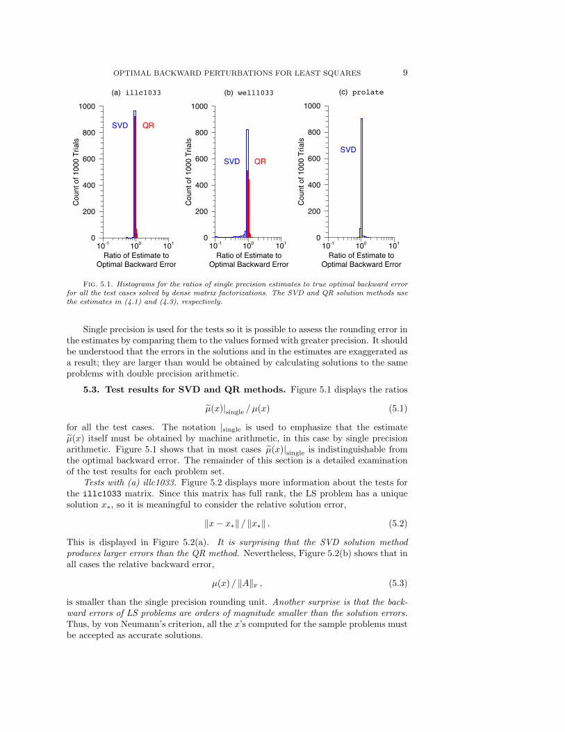
Fig. 5.1. Histograms for the ratios of single precision estimates to true optimal backward errorfor all the test cases solved by dense matrix factorizations. The SVD and QR solution methods usethe estimates in (4.1) and (4.3), respectively.

Single precision is used for the tests so it is possible to assess the rounding error inthe estimates by comparing them to the values formed with greater precision. It shouldbe understood that the errors in the solutions and in the estimates are exaggerated asa result; they are larger than would be obtained by calculating solutions to the sameproblems with double precision arithmetic.

5.3. Test results for SVD and QR methods. Figure 5.1 displays the ratios

µ(x)|single / µ(x) (5.1)

for all the test cases. The notation |single is used to emphasize that the estimateµ(x) itself must be obtained by machine arithmetic, in this case by single precisionarithmetic. Figure 5.1 shows that in most cases µ(x)|single is indistinguishable fromthe optimal backward error. The remainder of this section is a detailed examinationof the test results for each problem set.

Tests with (a) illc1033. Figure 5.2 displays more information about the tests forthe illc1033 matrix. Since this matrix has full rank, the LS problem has a uniquesolution x∗, so it is meaningful to consider the relative solution error,

‖x− x∗‖ / ‖x∗‖ . (5.2)

This is displayed in Figure 5.2(a). It is surprising that the SVD solution methodproduces larger errors than the QR method. Nevertheless, Figure 5.2(b) shows that inall cases the relative backward error,

µ(x) / ‖A‖F , (5.3)

is smaller than the single precision rounding unit. Another surprise is that the back-ward errors of LS problems are orders of magnitude smaller than the solution errors.Thus, by von Neumann’s criterion, all the x’s computed for the sample problems mustbe accepted as accurate solutions.


Fig. 5.2. For the illc1033 test cases, these figures show the relative size of: (a) solutionerror, (b) optimal backward error, (c, d, e) errors in the estimated optimal backward error. Thesequantities are defined in (5.2), (5.3), (5.4), (5.6), and (5.7), respectively.

The scatter away from 100 in Figure 5.1’s ratios is explained by the final threeparts of Figure 5.2. The overall discrepancy in µ(x)|single as compared to µ(x) isshown in Figure 5.2(c): ∣∣ µ(x)|single − µ(x)

∣∣ / µ(x) . (5.4)

This discrepancy is the sum of rounding error and approximation error:

µ(x)|single − µ(x) =[µ(x)|single − µ(x)

]︸︷︷︸rounding error

+[µ(x)− µ(x)

]︸︷︷︸approximation error

. (5.5)

Figure 5.2(d) shows the relative rounding error,∣∣ µ(x)|single − µ(x)∣∣ / µ(x) , (5.6)

while Figure 5.2(e) shows the relative approximation error,∣∣ µ(x)− µ(x)∣∣ / µ(x) . (5.7)

Yet another surprise from Figure 5.2(e) is that the approximation error of the esti-mate is vanishingly small. Evidently (1.6)’s limit approaches 1 so quickly that theapproximation error is by far the smaller quantity in (5.5). Thus the scatter in Figure5.1’s ratios is due primarily to rounding errors in evaluating the estimate.


Fig. 5.3. For the well1033 test cases, these figures show the relative size of: (a) solutionerror, (b) optimal backward error, (c, d, e) errors in the estimated optimal backward error. Thesequantities are defined in (5.2), (5.3), (5.4), (5.6), and (5.7), respectively.

As a result of this scatter, it should be pointed out, the computed estimate oftendoes not satisfy Gu’s lower bound in (1.5),

1 ≈ ‖r∗‖‖r‖

6≤µ(x)

∣∣single

µ(x).

The bound fails even when x and µ(x) are evaluated in double precision. For higherprecisions the scatter does decrease, but the lower bound becomes more stringentbecause r becomes a better approximation to r∗.

Tests with (b) well1033. Figure 5.3 shows the details of the tests for the betterconditioned matrix well1033. Some differences between it and Figure 5.2 can bepartially explained by the conditioning of LS problems. The relative, spectral-normcondition number of the full-rank LS problem is [3, p. 31, eqn. 1.4.28] [11, thm. 5.1](

‖r∗‖σmin(A) ‖x∗‖

+ 1

)κ2(A) . (5.8)

As A becomes better conditioned so does the LS problem, and the calculated solutionsshould become more accurate. This is the trend in the leftward shift of the histogramsfrom Figure 5.2(a) to 5.3(a).

However, the rightward shift from Figure 5.2(d) to 5.3(d) suggests that as xbecomes more accurate, µ(x) may become more difficult to evaluate accurately. The


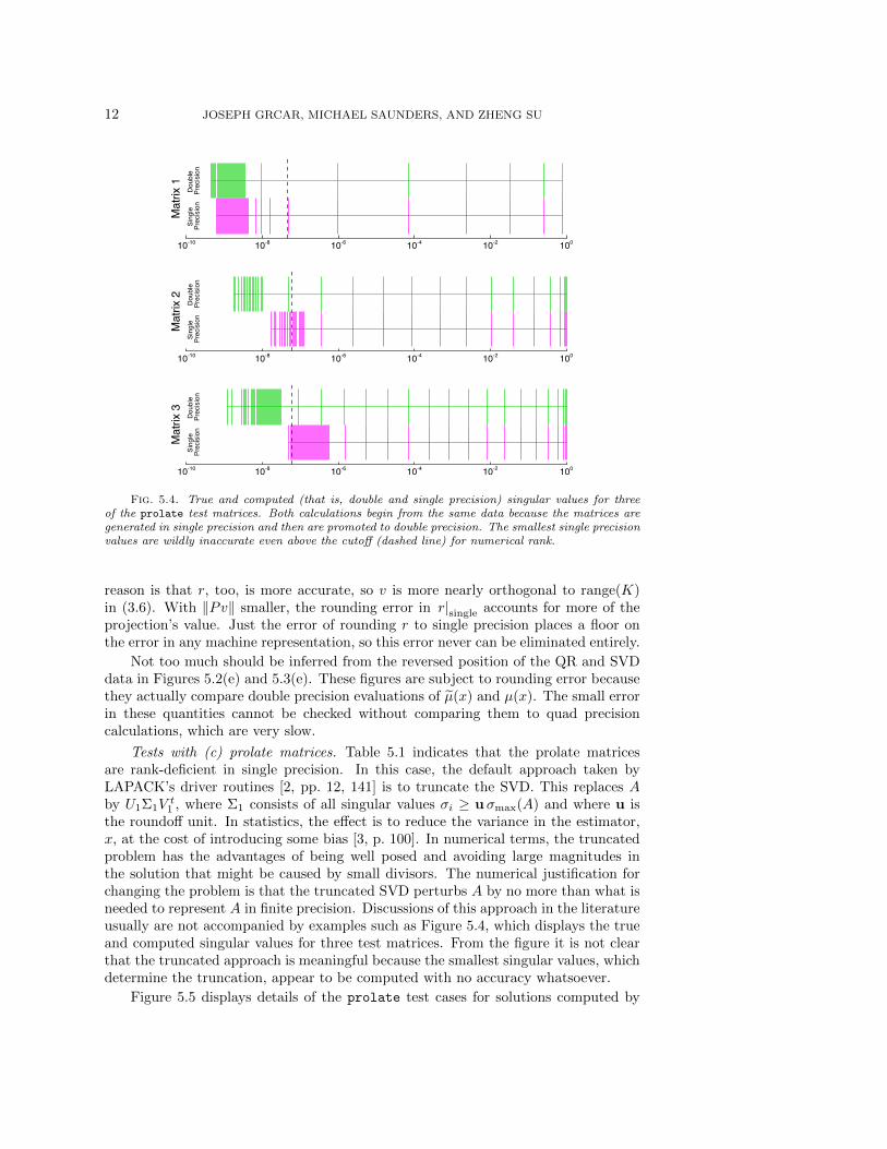
Fig. 5.4. True and computed (that is, double and single precision) singular values for threeof the prolate test matrices. Both calculations begin from the same data because the matrices aregenerated in single precision and then are promoted to double precision. The smallest single precisionvalues are wildly inaccurate even above the cutoff (dashed line) for numerical rank.

reason is that r, too, is more accurate, so v is more nearly orthogonal to range(K)in (3.6). With ‖Pv‖ smaller, the rounding error in r|single accounts for more of theprojection’s value. Just the error of rounding r to single precision places a floor onthe error in any machine representation, so this error never can be eliminated entirely.

Not too much should be inferred from the reversed position of the QR and SVDdata in Figures 5.2(e) and 5.3(e). These figures are subject to rounding error becausethey actually compare double precision evaluations of µ(x) and µ(x). The small errorin these quantities cannot be checked without comparing them to quad precisioncalculations, which are very slow.

Tests with (c) prolate matrices. Table 5.1 indicates that the prolate matricesare rank-deficient in single precision. In this case, the default approach taken byLAPACK’s driver routines [2, pp. 12, 141] is to truncate the SVD. This replaces Aby U1Σ1V

t1 , where Σ1 consists of all singular values σi ≥ uσmax(A) and where u is

the roundoff unit. In statistics, the effect is to reduce the variance in the estimator,x, at the cost of introducing some bias [3, p. 100]. In numerical terms, the truncatedproblem has the advantages of being well posed and avoiding large magnitudes inthe solution that might be caused by small divisors. The numerical justification forchanging the problem is that the truncated SVD perturbs A by no more than what isneeded to represent A in finite precision. Discussions of this approach in the literatureusually are not accompanied by examples such as Figure 5.4, which displays the trueand computed singular values for three test matrices. From the figure it is not clearthat the truncated approach is meaningful because the smallest singular values, whichdetermine the truncation, appear to be computed with no accuracy whatsoever.

Figure 5.5 displays details of the prolate test cases for solutions computed by


Fig. 5.5. For the prolate test cases, these figures show the relative size of: (a) solutionerror, (b) optimal backward error, (c, d, e) errors in the estimated optimal backward error. Thesequantities are defined in (5.2), (5.3), (5.4), (5.6), and (5.7), respectively.

the truncated SVD. The solution’s relative error in Figure 5.5(a) is with respect tothe unique solution of the LS problem, which does have full rank in higher precision.Although the single precision solutions are quite different from x∗, Figure 5.5(b)indicates that the backward errors are acceptably small. The small backward errorsdo justify using the truncated SVD to solve these problems. This suggests thatthe ability to estimate the backward error might be useful in designing algorithmsfor rank-deficient problems. For example, in the absence of a problem-dependentcriterion, small singular values might be included in the truncated SVD providedthey do not increase the backward error.

The rest of Figure 5.5 is consistent with the other tests. The rounding error inthe estimate has about the same relative magnitude, O(10−2), in all Figures 5.2(d),5.3(d), and 5.5(d). The approximation error shown in Figure 5.5(e) is larger thanin Figures 5.2(e) and 5.3(e) because of the much less accurate solutions, but overall,µ(x)|single remains an acceptable backward error estimate. Indeed, the estimate isremarkably good given the poor quality of the computed solutions.


6. Test results for iterative methods. In the preceding numerical results,the vector x has been an accurate estimate of the LS solution. Applying LSQR to aproblem minx ‖Ax− b‖ generates a sequence of approximate solutions {xk}. For thewell and illc test problems we used the Matlab code in section 4.4 to computeµ(xk) for each xk.

To our surprise, these values proved to be monotonically decreasing, as illustratedby the lower curve in Figures 6.1 and 6.2. (To make it scale-independent, this curveis really µ(xk)/‖A‖F.)

For each xk, let rk = b−Axk and η(xk) = ‖rk‖/‖xk‖. Also, let Kk, vk and yk bethe quantities in (3.1) when x = xk. The LSQR iterates have the property that ‖rk‖and ‖xk‖ are decreasing and increasing respectively, so that η(xk) is monotonicallydecreasing. Also, we see from (3.6) that

µ(xk) =‖Y tk vk‖‖xk‖

<‖vk‖‖xk‖

=‖rk‖‖xk‖

= η(xk),

so that η(xk) forms a monotonically decreasing bound on µ(x). However, we can onlynote empirically that µ(xk) itself appears to decrease monotonically also.

The stopping criterion for LSQR is of interest. It is based on a non-optimalbackward error ‖Ek‖F derived by Stewart [24], where

Ek = − 1

‖rk‖2rkr

tkA.

(If A = A+Ek and r = b− Axk, then (xk, rk) are the exact solution and residual forminx ‖Ax−b‖.) Note that ‖Ek‖F = ‖Ek‖2 = ‖Atrk‖/‖rk‖. On incompatible systems,LSQR terminates when its estimate of ‖Ek‖2/‖A‖F is sufficiently small; i.e., when

test2k ≡‖Atrk‖‖A‖k‖rk‖

≤ atol, (6.1)

where ‖A‖k is a monotonically increasing estimate of ‖A‖F and atol is a user-specifiedtolerance.

Figures 6.1 and 6.2 show ‖rk‖ and three relative backward error quantities forproblems well1033 and illc1033 when LSQR is applied to minx ‖Ax − b‖ withatol = 10−12. From top to bottom, the curves plot the following (log10):

• ‖rk‖ (monotonically decreasing).• test2k, LSQR’s relative backward error estimate (6.1).• η(xk)/‖A‖F, the optimal relative backward error for Ax = b (monotonic).• µ(xk)/‖A‖F, the KW relative backward error estimate for minx ‖Ax − b‖,

where µ(xk) = ‖Pvk‖/‖xk‖ in (3.6) is evaluated as in section 4.4. (It isapparently monotonic.)

The last curve is extremely close to the optimal relative backward error for LS prob-lems. We see that LSQR’s test2k is two or three orders of magnitude larger formost xk, and it is far from monotonic. Nevertheless, its trend is downward in broadsynchrony with µ(xk)/‖A‖F. We take this as an experimental approval of Stewart’sbackward error Ek and confirmation of the reliability of LSQR’s cheaply computedstopping rule.


Fig. 6.1. Backward error estimates for each LSQR iterate xk during the solution of well1033with atol = 10−12. The middle curve is Stewart’s estimate as used in LSQR; see (6.1). The bottomcurve is µ(xk)/‖A‖F , where µ(xk) is the KW bound on the optimal backward error computed as insection 4.4 (unexpectedly monotonic).

Fig. 6.2. Backward error estimates for each LSQR iterate xk during the solution of illc1033with atol = 10−12.


6.1. Iterative computation of µ(x). Here we use an iterative solver twice:first on the original LS problem to obtain an approximate solution x, and then on theassociated KW problem to estimate the backward error for x.

1. Apply LSQR to minx ‖Ax − b‖ with iteration limit kmax . This generates asequence {xk}, k = 1 : kmax . Define x = xkmax . We want to estimate thebackward error for that final point x.

2. Define r = b−Ax and atol = 0.01‖Atr‖/(‖A‖F‖x‖).3. Apply LSQR to the KW problem miny ‖Ky − v‖ (4.4) with convergence

tolerance atol. As described in section 4.5, this generates a sequence ofestimates µ(x) ≈ ‖z`‖/‖x‖ using ‖z`‖ ≈ ‖Ky‖ in (4.5)–(4.6).

To avoid ambiguity we use k and ` for LSQR’s iterates on the two problems. Also,the following figures plot relative backward errors µ(x)/‖A‖F, even though the ac-companying discussion doesn’t mention ‖A‖F.

For problem well1033 with kmax = 50, Figure 6.3 shows µ(xk) for k = 1 : 50(the same as the beginning of Figure 6.1). The right-hand curve then shows about130 estimates ‖z`‖/‖x‖ converging to µ(x50) with about 2 digits of accuracy (becauseof the choice of atol).

Similarly with kmax = 160, Figure 6.4 shows µ(xk) for k = 1 : 160 (the same asthe beginning of Figure 6.1). The final point x160 is close to the LS solution, and thesubsequent KW problem converges more quickly. About 20 LSQR iterations give a2-digit estimate of µ(x160).

For problem illc1033, similar effects were observed. In Figure 6.5 about 2300iterations on the KW problem give a 2-digit estimate of µ(x2000), but in Figure 6.6only 280 iterations are needed to estimate µ(x3500).

6.2. Comparison with Malyshev and Sadkane’s iterative method. Maly-shev and Sadkane [16] show how to use the bidiagonalization of A with starting vectorr to estimate σmin[A B] in (1.1). This is the same bidiagonalization that LSQR useson the KW problem (3.1) to estimate µ(x). The additional work per iteration isnominal in both cases. A numerical comparison is therefore of interest. We use theresults in Tables 5.2 and 5.3 of [16] corresponding to LSQR’s iterates x50 and x160 onproblems well1033 and illc1033. Also, Matlab gives us accurate values for µ(xk)and σmin[A B] via sparse qr (section 4.4) and dense svd respectively.

In Tables 6.1–6.3, the true backward error is µ(x) = σmin[A B], the last line ineach table.

In Tables 6.1–6.2, σ` denotes Malyshev and Sadkane’s σmin(B`) [16, (3.7)]. Notethat the iterates σ` provide decreasing upper bounds on σmin[A B], while the LSQRiterates ‖z`‖/‖x‖ are increasing lower bounds on µ(x), but they do not bound σmin.

We see that all of the Malyshev and Sadkane estimates σ` bound σmin to withina factor of 2, but they have no significant digits in agreement with σmin. In contrast,η(xk) agrees with σmin to 3 digits in three of the cases, and indeed it provides a tighterbound whenever it satisfies η < σ`. The estimates σ` are therefore more valuable whenη > σmin (i.e., when xk is close to a solution x∗).

However, we see that LSQR computes µ(xk) with 3 or 4 correct digits in all cases,and requires fewer iterations as xk approaches x∗. The bottom-right values in Tables6.1 and 6.3 show Grcar’s limit (1.6) taking effect. LSQR can compute these values tohigh precision with reasonable efficiency.

The primary difficulty with our iterative computation of µ(x) is that when x isnot close to x∗, rather many iterations may be required, and there is no warning thatµ may be an underestimate of µ.


Fig. 6.3. Problem well1033: Iterative solution of KW problem after LSQR is terminated at x50.

Fig. 6.4. Problem well1033: Iterative solution of KW problem after LSQR is terminated at x160.


Fig. 6.5. Problem illc1033: Iterative solution of KW problem after LSQR is terminated at x2000.

Fig. 6.6. Problem illc1033: Iterative solution of KW problem after LSQR is terminated at x3500.


Table 6.1Comparison of σ` and ‖z`‖/‖xk‖ for problem well1033.

k = 50

‖rk‖ 6.35e+1

‖Atrk‖ 5.04e+0

η(xk) 7.036807e−3

atol 4.44e−5

` σ` ‖z`‖/‖xk‖10 2.35e−2 2.11e−3

50 1.51e−2 5.43e−3

100 1.22e−2 6.32e−3

127 6.379461e−3

µ(xk) 6.379462e−3

σmin[A B] 7.036158e−3

k = 160

‖rk‖ 7.52e−1

‖Atrk‖ 4.49e−4

η(xk) 7.3175e−5

atol 3.34e−7

` σ` ‖z`‖/‖xk‖10 3.79e−5 8.9316e−8

19 8.9381e−8

50 2.95e−7

100 1.21e−7

µ(xk) 8.9386422278e−8

σmin[A B] 8.9386422275e−8

Table 6.2Comparison of σ` and ‖z`‖/‖xk‖ for problem illc1033.

k = 50

‖rk‖ 3.67e+1

‖Atrk‖ 3.08e+1

η(xk) 4.6603e−3

atol 4.69e−5

` σ` ‖z`‖/‖xk‖10 3.04e−2 1.62e−3

50 1.84e−2 3.71e−3

100 1.02e−2 4.11e−3

200 4.25e−3

300 4.28e−3

310 4.2825e−3

µ(xk) 4.2831e−3

σmin[A B] 4.6576e−3

k = 160

‖rk‖ 1.32e+1

‖Atrk‖ 3.78e−1

η(xk) 1.6196e−3

atol 1.60e−5

` σ` ‖z`‖/‖xk‖10 1.10e−2 2.09e−4

50 4.63e−3 4.92e−4

100 3.40e−3 8.45e−4

200 1.23e−3

300 1.34e−3

400 1.38e−3

500 1.3841e−3

542 1.3843e−3

µ(xk) 1.3847e−3

σmin[A B] 1.6144e−3

Ironically, solving the KW problem for x = xk is akin to restarting LSQR on aslightly modified problem. We have observed that if ` iterations are needed on theKW problem to estimate µ(xk)/‖A‖F, continuing the original LS problem a further `iterations would have given a point xk+` for which the Stewart-type backward errortest2k+` is generally at least as small. (Compare Figures 6.2 and 6.6.) Thus, thedecision to estimate optimal backward errors by iterative means must depend on thereal need for optimality.

7. Conclusions. Several approaches have been suggested and tested to evaluatean estimate for the optimal size (that is, the minimal Frobenius norm) of backwarderrors for LS problems. Specifically, to estimate the true backward error µ(x) in (1.1)(for an arbitrary vector x), we have studied the estimate µ(x) in (1.3). The numericaltests support various conclusions as follows.


Table 6.3‖z`‖/‖xk‖ for problem illc1033.

k = 2000

‖rk‖ 7.89e−1

‖Atrk‖ 2.45e−3

η(xk) 7.82e−5

atol 1.73e−6

` ‖z`‖/‖xk‖500 1.22e−5

1000 1.81e−5

1500 1.97e−5

2000 2.02e−5

2330 2.08e−5

µ(xk) 2.10e−5

σmin[A B] 2.12e−5

k = 3500

‖rk‖ 7.52e−1

‖Atrk‖ 5.54e−8

η(xk) 7.30e−5

atol 4.11e−11

` ‖z`‖/‖xk‖10 4.41e−11

50 1.11e−10

100 1.54e−10

200 2.28e−10

280 2.32006e−10

µ(xk) 2.3209779030e−10

σmin[A B] 2.3209779099e−10

Regarding LS problems themselves:1. The QR solution method results in noticeably smaller solution errors than

the SVD method.2. The optimal backward errors for LS problems are much smaller—often orders

of magnitude smaller—than the solution errors.

Regarding the estimates:3. The computed estimate of the optimal backward error is very near the true

optimal backward error in all but a small percent of the tests.(a) Grcar’s limit (1.6) for the ratio of the estimate to the optimal backward

error appears to approach 1 very quickly.(b) The greater part of the fluctuation in the estimate is caused by rounding

error in its evaluation.4. Gu’s lower bound (1.5) for the ratio of the estimate to the optimal back-

ward error often fails in practice because of rounding error in evaluating theestimate.

5. As the computed solution of the LS problem becomes more accurate, theestimate may become more difficult to evaluate accurately because of theunavoidable rounding error in forming the residual.

6. For QR methods, evaluating the estimate is insignificant compared to thecost of solving a dense LS problem.

7. When iterative methods become necessary, applying LSQR to the KW prob-lem is a practical alternative to the bidiagonalization approach of Malyshevand Sadkane [16], particularly when x is close to x∗. No special coding isrequired (except a few new lines in LSQR to compute ‖zk‖ ≈ Ky as in sec-tion 4.5), and LSQR’s normal stopping rules ensure at least some good digitsin the computed µ(x).

8. The smooth lower curves in Figures 6.1 and 6.2 suggest that when LSQR isapplied to an LS problem, the optimal backward errors for the sequence ofapproximate solutions {xk} are (unexpectedly) monotonically decreasing.

9. The Stewart backward error used in LSQR’s stopping rule (6.1) can be someorders of magnitude larger than the optimal backward error, but it appearsto track the optimal error well.


REFERENCES

[1] M. Adlers. Topics in Sparse Least Squares Problems. PhD thesis, Linkoping University, Sweden,2000.

[2] E. Anderson, Z. Bai, C. Bischof, J. Demmel, J. Dongarra, J. Du Croz, A. Greenbaum, S. Ham-marling, A. McKenney, S. Ostrouchov, and D. Sorensen. LAPACK Users’ Guide. Societyfor Industrial and Applied Mathematics, Philadelphia, 1992.

[3] A. Bjorck. Numerical Methods for Least Squares Problems. Society for Industrial and AppliedMathematics (SIAM), Philadelphia, 1996.

[4] R. F. Boisvert, R. Pozo, K. Remington, R. Barrett, and J. Dongarra. The Matrix Market: aweb repository for test matrix data. In R. F. Boisvert, editor, The Quality of NumericalSoftware, Assessment and Enhancement, pages 125–137. Chapman & Hall, London, 1997.The web address of the Matrix Market is http://math.nist.gov/MatrixMarket/.

[5] G. Calafiore, F. Dabbene, and R. Tempo. Radial and uniform distributions in vector and matrixspaces for probabilistic robustness. In D. E. Miller et al., editor, Topics in Control andIts Applications, pages 17–31. Springer, 2000. Papers from a workshop held in Toronto,Canada, June 29–30, 1998.

[6] J. J. Dongarra, J. R. Bunch, C. B. Moler, and G. W. Stewart. LINPACK Users’ Guide. Societyfor Industrial and Applied Mathematics (SIAM), Philadelphia, 1979.

[7] I. S. Duff, R. G. Grimes, and J. G. Lewis. Sparse matrix test problems. ACM Transactions onMathematical Software, 15(1):1–14, 1989.

[8] G. H. Golub and W. Kahan. Calculating the singular values and pseudoinverse of a matrix.SIAM Journal on Numerical Analysis, 2:205–224, 1965.

[9] G. H. Golub and C. F. Van Loan. Matrix Computations. The Johns Hopkins University Press,Baltimore, second edition, 1989.

[10] J. F. Grcar. Differential equivalence classes for metric projections and optimal backward errors.Technical Report LBNL-51940, Lawrence Berkeley National Laboratory, 2002. Submittedfor publication.

[11] J. F. Grcar. Optimal sensitivity analysis of linear least squares. Technical Report LBNL-52434,Lawrence Berkeley National Laboratory, 2003. Submitted for publication.

[12] M. Gu. Backward perturbation bounds for linear least squares problems. SIAM Journal onMatrix Analysis and Applications, 20(2):363–372, 1999.

[13] M. Gu. New fast algorithms for structured linear least squares problems. SIAM Journal onMatrix Analysis and Applications, 20(1):244–269, 1999.

[14] N. J. Higham. Accuracy and Stability of Numerical Algorithms. Society for Industrial andApplied Mathematics, Philadelphia, second edition, 2002.

[15] R. Karlson and B. Walden. Estimation of optimal backward perturbation bounds for the linearleast squares problem. BIT, 37(4):862–869, December 1997.

[16] A. N. Malyshev and M. Sadkane. Computation of optimal backward perturbation bounds forlarge sparse linear least squares problems. BIT, 41(4):739–747, December 2002.

[17] P. Matstoms. Sparse QR factorization in MATLAB. ACM Trans. Math. Software, 20:136–159,1994.

[18] J. von Neumann and H. H. Goldstine. Numerical inverting of matrices of high order. Bulletinof the American Mathematical Society, 53(11):1021–1099, November 1947. Reprinted in[?, v. 5, pp. 479–557].

[19] W. Oettli and W. Prager. Compatibility of approximate solution of linear equations with givenerror bounds for coefficients and right-hand sides. Num. Math., 6:405–409, 1964.

[20] C. C. Paige and M. A. Saunders. LSQR: An algorithm for sparse linear equations and sparseleast squares. ACM Trans. Math. Software, 8(1):43–71, 1982.

[21] C. C. Paige and M. A. Saunders. Algorithm 583; LSQR: Sparse linear equations and least-squares problems. ACM Trans. Math. Software, 8(2):195–209, 1982.

[22] M. A. Saunders. Computing projections with LSQR. BIT, 37(1):96–104, 1997.[23] M. A. Saunders. lsqr.f, lsqr.m. http://www.stanford.edu/group/SOL/software/lsqr.html, 2002.[24] G. W. Stewart. Research development and LINPACK. In J. R. Rice, editor, Mathematical

Software III, pages 1–14. Academic Press, New York, 1977.[25] Z. Su. Computational Methods for Least Squares Problems and Clinical Trials. PhD thesis,

Stanford University, 2005.[26] J. M. Varah. The prolate matrix. Linear Algebra Applicat., 187:269–278, 1993.[27] B. Walden, R. Karlson, and J.-G. Sun. Optimal backward perturbation bounds for the linear

least squares problem. Numerical Linear Algebra with Applications, 2(3):271–286, 1995.

Documents

ESTIMATES OF OPTIMAL BACKWARD PERTURBATIONS FOR