This is a repository copy of Estimating an EQ-5D population value set: the case of Japan.

White Rose Research Online URL for this paper:http://eprints.whiterose.ac.uk/105364/

Version: Accepted Version

Article:

Tsuchiya, A. orcid.org/0000-0003-4245-5399, Ikeda, S., Ikegami, N. et al. (6 more authors)(2002) Estimating an EQ-5D population value set: the case of Japan. Health Economics, 11 (4). pp. 341-353. ISSN 1057-9230

https://doi.org/10.1002/hec.673

eprints@whiterose.ac.ukhttps://eprints.whiterose.ac.uk/

Reuse

Unless indicated otherwise, fulltext items are protected by copyright with all rights reserved. The copyright exception in section 29 of the Copyright, Designs and Patents Act 1988 allows the making of a single copy solely for the purpose of non-commercial research or private study within the limits of fair dealing. The publisher or other rights-holder may allow further reproduction and re-use of this version - refer to the White Rose Research Online record for this item. Where records identify the publisher as the copyright holder, users can verify any specific terms of use on the publisher’s website.

Takedown

If you consider content in White Rose Research Online to be in breach of UK law, please notify us by emailing eprints@whiterose.ac.uk including the URL of the record and the reason for the withdrawal request.

1

June 2001: ver 4.3; for re-submission to Health Economics

Estimating an EQ-5D population value set: The case of Japan

Aki Tsuchiya, Shunya Ikeda, Naoki Ikegami, Shuzo Nishimura, Ikuro Sakai,

Takashi Fukuda, Chisato Hamashima, Akinori Hisashige, Makoto Tamura

Aki Tsuchiya (corresponding author), PhD; Research Associate, School of Health and Related Research, University of Sheffield, Sheffield, UK Shunya Ikeda, MD MSc DrMedSci; Assistant Professor, Dept. of Health Policy and Management, Keio University School of Medicine, Tokyo, Japan Naoki Ikegami, MD MA DrMedSci; Professor and Chair, Dept. of Health Policy and Management, Keio University School of Medicine, Tokyo, Japan Shuzo Nishimura, PhD; Professor, Graduate School of Economics, Kyoto University, Kyoto, Japan Ikuro Sakai, MS; Faculty of Medicine, The University of Tokyo, Tokyo, Japan Takashi Fukuda, PhD; Associate Professor, Dept. of Pharmacoeconomics, Graduate School of Pharmaceutical Sciences, The University of Tokyo, Tokyo, Japan Chisato Hamashima, MD DrMedSc; Lecturer, Dept. of Preventive Medicine, St.Mariannna University School of Medicine, Kawasaki, Japan Akinori Hisashige, MD PhD; Professor, Dept. of Preventive Medicine, School of Medicine, University of Tokushima, Tokushima, Japan Makoto Tamura, PhD; Professor, International University of Health and Welfare, Otawara, Japan

2

C o r r e s p o n d i n g a u t h o r :

Aki Tsuchiya, SHEG, ScHARR, University of Sheffield, 30 Regent Street, Sheffield, S1 4DA e-mail: a.tsuchiya@sheffield.ac.uk Tel: 0114.222.0710 Fax: 0114.272.4095

A c k n o w l e d g e m e n t s

This study has been funded by Glaxo-Wellcome and Pharmacia & Upjohn. Most

helpful comments were offered, amongst others, by Paul Dolan, Paul Kind, Shigeki

Nawata, Nigel Rice, Jenny Roberts, Hiroyuki Sakamaki, and Alan Williams.

Preliminary results of this study have been presented to the International Society for

Quality of Life Research (ISOQOL) meeting, Barcelona, November 1999, and to the

EuroQol meeting, Sitges, November 1999. Special thanks are to those respondents

who agreed to be interviewed. The usual disclaimer applies.

3

Estimating an EQ-5D population value set:

The case of Japan

Key words: EQ-5D, population values, QALYs, health status measurement, TTO

Abstract length: 199 words

length of main text: 5,680 words

number of figures: 3

number of tables: 5

4

A b s t r a c t

Quality adjustment weights for quality-adjusted life years (QALYs) are available with

the EQ-5D Instrument, which are based on a survey that quantified the preferences of

the British public. However, the extent to which this British value set is applicable to

other, especially non-European, countries is yet unclear. The objectives of this study

are (a) to compare the valuations obtained in Japan and Britain, and (b) to explore a

local Japanese value set. A diminished study design is employed, where 17

hypothetical EQ-5D health states are evaluated as opposed to 42 in the British study.

The official Japanese version of the instrument and the Time Trade-Off method are

used to interview 543 members of the public. The results are: firstly, the evaluations

obtained in Japan and those from Britain differ by 0.24 on average on a [-1, +1] scale,

and mean absolute error (MAE) in predicting the Japanese preferences with the British

value set is 0.23. Secondly, comparable regressions suggest that the two peoples have

systematically different preference structures (p < 0.001 for 8 of 12 coefficients; F-test).

Thirdly, using alternative models, the predictions are improved so that the local

Japanese value set achieves MAE in the order of 0.01.

5

1 . I n t r o d u c t i o n a n d b a c k g r o u n d

To satisfy the growing demand for health care technology assessments using CEAs

(cost-effectiveness analyses) from the societal perspective[1], a set of population

values for different health states is necessary. A CEA from this perspective may

employ QALYs (quality-adjusted life years) as the outcome measure, with quality

adjustment weights derived from the preferences of the general public. A social value

set is estimated for a given health states classification system, and is a table of all

possible health states of this system with their corresponding values, generated from

the public. These values are numbers on a scale with 1 for full health and 0 for being

dead: a positive (negative) number implies that the health state is better (worse) than

dead. These numbers are assumed to satisfy interval scale properties, and serve as

quality adjustment weights in QALYs.

The method to estimate a value set involves the following steps:

(1) systematic description of health states, by dimensions and levels,

(2) selection of a subset of health states from all the possible health states,

(3) quantification of the preferences of members of the public regarding the

subset states, and

(4) modelling the obtained preference data so as to predict the preference

regarding the remaining health states.

Regarding the number of health states identifiable by the descriptive system there is

6

a potential conflict between the sensitivity of the value set and the feasibility and

reliability of the valuation task. If the number of health states is small, the task of

generating a value set will be relatively easy (at the extreme, all states can be directly

valued, so that the second and fourth stages above will be redundant, as is the case with

the so-called Rosser-Kind Index[2]), but the resulting value set may be too crude to

discriminate amongst the plethora of different health states. On the other hand, the

larger the number of health states, the descriptive system can be expected (though not

necessarily) to distinguish health states with more subtlety, but the task of producing a

value set will become increasingly more taxing.

A similar conflict is present at the second stage, regarding the selection of the subset

of heath states to be evaluated by the respondents. (Note that these health states are

“hypothetical” since the respondents are not actually in these states, but are asked to

imagine themselves in one or another.) On the one hand, given a descriptive system,

the higher the ratio of the subset for evaluation to the entire set of all possible health

states described by the instrument, the more robust one can expect the modelling

exercise to be, and vice versa. On the other hand, the higher this ratio, and therefore

the larger the number of health states to be directly valued, the more onerous becomes

the evaluation exercise.

The third and fourth stages can be carried out in two ways[3]. One is to present

7

health states at stage three as “decomposed” states, by specifying a level on a particular

dimension without referring to the other dimensions. Preferences thus obtained will

then be modelled in the fourth stage based on multi-attribute utility theory[4]. The

other is to present “composite” states, by specifying levels on all dimensions, and then

modelling will be based on statistical inference.

From 1987 to 1995, the Centre for Health Economics, University of York, carried

out a research project entitled the Measurement and Valuation of Health (MVH)[3, 5,

6] to produce a population value set. To describe the health states, they used the

EQ-5D Instrument, which has 5 dimensions with 3 levels in each (see Figure 1)[7].

To quantify people’s preferences, they used the so-called TTO-prop method[8]. This

is a type of TTO (Time Trade-Off; explained below in 2.4.2.) that uses a “time board”

as a visual aid. The modelling method used was based on statistical inference (and

thus the health states were presented as “composite” states). The main product of the

MVH project was a EQ-5D value set based on TTO data obtained from 2997

respondents systematically covering a pool of 42 EQ-5D health states.

The objective of the present study was firstly to examine whether this British social

value set is applicable in Japan, by comparing, for selected hypothetical health states,

valuations obtained from the Japanese public with British values. Should this

demonstrate a wide discrepancy, the second task then was to estimate a social value set

8

for Japanese use. To date, there are no local value sets offered in Japan by any

HRQOL instrument, nor has the appropriateness of applying the EQ-5D British value

set been examined. This study will either establish the latter, or offer the former, and

is thereby expected to contribute to the tools available for health care technology

assessments in Japan.

In addition to the above objectives, the study also addressed a methodological issue.

The main difficulty in replicating the MVH study is its size: the large number of

EQ-5D health states evaluated, and its factorial design, inevitably requires a large

number of respondents. If it can be demonstrated that EQ-5D population value sets

of comparable goodness of fit can be estimated from a fewer number of health states,

and therefore smaller number of respondents, this will mostly likely promote the

examination of the appropriateness of applying the MVH value set in different

locations and populations, and, where appropriate, the estimation of a local value set.

This study, therefore, employed a “modified” version of the MVH protocol[9].

2 . M e t h o d s

2.1 The hypothetical health states and their quantification

The present study is a quasi-replication of the MVH study, following the “modified”

9

protocol. More specifically, instead of the original factorial design, where each

respondent values a different subset of a pool of hypothetical health states, all

respondents were presented with the same set of 17 health states (cf. Table 2). These

states have been selected from the set of 42 states used in the MVH study, by the

researchers at the University of York, as the minimum set of health states needed to

estimate the value set[9].

The Japanese version of the EQ-5D Instrument has been translated from the English

original following the translation procedures set by the EuroQol Group, which involve

forward translations, backward translations, and consultations with lay panels. For a

detailed report and discussion of the translation process see elsewhere[10, 11].

Further, the TTO procedure and manual used in the MVH study[8] were translated into

Japanese by the authors.

2.2. Data collection

2.2.1 The sample

In three Prefectures, Saitama, Hiroshima and Hokkaido, people aged 20 and above

were sampled for the survey. A 2-stage random sampling method was used by (a)

randomly selecting 62 of the smallest geographical units within each Prefecture, and

then (b) randomly selecting individuals from the local registry of electorates of the

10

geographical unit. Brief letters inviting the addressees to participate in the survey

were sent out, and then trained interviewers visited and interviewed the individuals at

their homes in August and September of 1998. For logistic convenience, one

interviewer was assigned to each geographical unit.

2.2.2 The interview procedure

Each interview consisted of the following:

(1) the standard EQ-5D questionnaire, which consists of:

(a) self-reported health in the 5-dimension descriptive system (EQ-5D),

(b) self-reported health on a visual analogue scale (VAS),

(c) VAS evaluations of 14 hypothetical health states expressed in EQ-5D,

(d) socio-economic background questions;

(2) ranking of 19 hypothetical health states expressed in EQ-5D, and

(3) TTO evaluation of the 17 hypothetical health states.

The 14 hypothetical health states evaluated by VAS at stage (1.c.) are dictated by the

standard EQ-5D Instrument, and, though there are some overlaps, are independent

from those valued in the later parts. The 19 hypothetical health states in the ranking

exercise in part (2) are the 17 used in the TTO, with the additional states “11111” and

“dead”. These two states are used as anchoring points (11111=1, and dead =0) in the

TTO exercise, and thus are not evaluated in part (3).

This paper is based mostly on the results obtained from part (3). A paper

11

concerning parts (1.a.) and (1.b.) is available[12], and another for part (1.c.)[13].

2.2.3 Exclusion criteria

The same 4 exclusion criteria as those adopted in the MVH study were used in this

study, which are:

completely missing TTO data,

only 1 or 2 states valued,

all states given the same value, and

all states valued as worse than dead.

While excluding respondents corresponding to the first and second category is not

problematic, excluding those in the third and fourth categories needs some justification.

The two central assumptions behind the whole exercise are, other things being equal,

that people prefer to live longer than not, and that people prefer to live in better health

than not; and these granted, the objective of the exercise is to elicit the trade-off

between quantity and quality of life. However, respondents, who either by

misunderstanding or by deliberate choice, fall in the third and/or fourth exclusion

categories are not trading quantity of life off for quality of life, or vice versa. There

are two issues. The first is, whether or not their responses can be taken at face value:

do respondents that satisfy the third exclusion criterion sincerely think that, for

example, delaying a death by an hour is worth infinitely more than curing a non-fatal

12

but severe and chronic pain? Do respondents corresponding to the fourth criterion

have no interest in avoiding death, or in health and health care in general? The

second issue is, while the respondents may well hold such views, whether it is

appropriate to include these into an analysis where the objective is to establish the

relative values of different levels of health for use in health care priority setting. In

other words, the reason for excluding these respondents is because, unless the

respondents have misunderstood the task, their responses are not engaging in the

exercise we present, and do not represent the kind of preference to be elicited here.

2.2.4 Adjusting TTO responses

For a given health state better than dead, a “10-year” TTO elicits the number of

years, t (< 10), where the respondent is indifferent between the following two

prospects:

to live in full health for t years, and

to live in the state in question for 10 years.

For a state worse than dead, it elicits the value of t (< 10) where the respondent is

indifferent between the two prospects:

to live in the state in question for t years and then in full health for 10 - t years,

and

13

immediate death.

The responses thus derived need to be “adjusted” so that they lie within the boundary

of –1 and +1, with 0 equivalent to dead. Conventionally, this is done by:

10/th , for states better than dead, and

110

t

h , for states worse than dead,

where t represents the obtained response and h the adjusted TTO value[14]. This

study used 10 years as the reference duration, and 6 months as the smallest unit of

measurement.

2.3 The analysis

2.3.1 Quality of the data

Apart from descriptions of averages and variances, the nature of the data is explored

in two ways: one within respondents, and the other across respondents. These offer

indirect evidence regarding whether or not the respondents understood the evaluation

task.

Since the hypothetical health states are described in the EQ-5D descriptive system,

“logical consistency” can be tested within each respondent. Logical consistency

concerns a given pair of health states: if one state of a pair is better than the other in at

least one dimension and not worse in any other, then the valuation for the former state

14

must be at least as good as the valuation for the later state. It is reasonable to

interpret that if whether or not a given respondent is inconsistent regarding two health

states is correlated to some indicator representing how easy or difficult it is to detect

the logical ordering between these two states, or “distance” between the states, then the

observed inconsistencies of this respondent represent some measurement or perception

error, while on the other hand if the inconsistencies are observed at random, then the

respondent may not have understood the valuation task. Further, inconsistency can be

defined in its weak form (allowing ties) and its strong form (not allowing ties). If, for

a given respondent, the difference between the number of violations of strong

inconsistency and of weak inconsistency is also correlated to distance, so that closer

states are more likely to be ties than farther states, this again suggests random error.

To the contrary, if no relationship is observed, this will be indirect evidence that the

respondent did not understand the valuation task. In this study, the “city block”

method was used as a crude approximation of “easiness”. This, for a pair of states, is

calculated by subtracting the corresponding levels of one state from the other, and then

adding them across dimensions. The maximum distance is between 11111 and 33333,

which is 2+2+2+2+2=10.

Further, the distribution of the rank order coefficients between individual TTO

responses and average TTO was studied. This can then be used to test the null

15

hypothesis: that there is no rank order correlation between the TTO values of each

individual respondent and the average TTO values of the group as a whole.

2.3.2 Comparison with the MVH value set

In order to test whether or not the British and Japanese have comparable

health-related preferences, the regression model used to estimate the British value set[3,

6] was applied to the Japanese data and the coefficients were compared. The

regressions were based on individual data. Adjusted TTO score h of each health state

by each respondent was subtracted from 1, and then these were regressed to 11 dummy

variables pertaining to the health state evaluated so that:

yh 1 ,

eNxy dldlld 3 ,

where dlx represents ten dummy variables that indicate the presence of either a level

2 or a level 3 in a given dimension of the evaluated state. In other words, d stands for

the dimensions: M for mobility, SC for self-care, UA for usual activities, PD for pain or

discomfort, AD for anxiety or depression; and l stands for either level 2 or level 3.

Since the objective of the exercise is to estimate a function that maps the 5-digit

description to average TTO, these ten dlx dummy variables form the core of the

regression. N3 is a dummy that is “on” when there is at least one dimension at level 3,

16

and “off” when there are none. This particular specification is referred to as the “N3

model” after this additional variable.

For example, the estimated equation for state 23111 is:

eNxxy SCSCMM 33322 . All health states (except 11111) indicate

some departure from full health (=11111), and given that this has the value of 1,

subtracting h from 1 represents the decrease in value each adverse state entails. The

intercept stands for the loss implied by any diversion from full health.

The comparison with the British results was carried out in two ways. One is by

comparing the coefficients of the Japanese N3 model with those of the original MVH

study where the regression is based on valuation data on 42 health states[3]. The

other is by comparing them with the coefficients where the regression is based on a

subset of the MVH data, limited to the valuation of the 17 health states used here[9].

2.3.3 Estimation method

Since each respondent was expected to have a different pattern of response, for

example, to offer higher or lower values than the average persistently across all health

states, a random effects (RE) estimation or a fixed effects (FE) estimation may be used

as estimation methods. Therefore, a series of preliminary analyses was carried out to

compare the simple ordinary least squares (OLS) regressions with RE and FE

17

regressions (statistic package STATA ver.6.0 was used). While the use of RE and FE

demonstrated that there are significant respondents effects (p < 0.001), and standard

errors are smaller, at the same time the p-values under the simple OLS regression are

already smaller than 0.001, and the changes in the dl coefficients across the three

estimation methods are less than 0.001.

As is explained below in section 3.1, the set of respondents providing data for the

analyses was not representative of the Japanese population in terms of age and sex

distribution, and therefore corrective weights were introduced for the estimation of the

population value set. The inclusion of corrective weights in the OLS regressions was

found to affect the dl coefficients by up to 0.002 (cf. Table 3). While corrective

weights can be used in OLS, their use is incompatible with RE and FE estimations in

STATA (ver.6.0). A choice therefore had to be made between accepting the

non-representativeness of the sample and to use RE or FE, or to incorporate corrective

weights and to use OLS. Since the corrective weights had a larger effect on the

coefficients relative to the RE and FE models, and since, as stated above, the p-values

under OLS were small enough, the choice made was to carry out the main analysis by

simple OLS regressions without accounting for respondent effects. The same applies

to the other models mentioned below.

18

2.3.4 Alternative models

To explore possibilities other than the N3 model, other additive models were

estimated. Given the objective of the exercise (to generate a mapping from the

5-digit descriptions to TTO values), the obvious candidate was the simple main effects

model, with the ten xdl dummies but without the N3 variable. Then the next step was

to include various interactive terms. However, the number of possible interactive

terms is very large, and therefore these were represented by the following proxy

variables:

N3: whether there is any dimension on level 3,

C3: the number of dimensions on level 3,

C3sq: the square of the number of dimensions on level 3,

N1: whether there is any dimension on level 1,

C1: the number of dimensions on level 1, and

C1sq: the square of the number of dimensions on level 1.

Models with different combinations of up to three of these additional interactive terms

(i.e. 6C1 + 6C2 + 6C3 = 6 + 15 + 20 = 41 models) were estimated. For example, a

“C3+N1+C1sq model” represents the regression equation:

esqCNCxy dldlld 113 321 . The same set of regressions was

also run without the intercept (i.e. Į = 0).

19

2.3.5 Comparison between alternative models

The performance of alternative models and the N3 model were compared in two

ways. First, goodness of fit for the 17 health states was analysed out by comparing

the values “predicted” from the models with the observed values. Smaller the mean

absolute error (MAE) the better, and there should be no systematic bias over severity.

In other words, there should be no over- or under-predictions correlated with the level

of quality of life. Given that there are only 17 points to predict, making statistical

testing difficult, the bias was tested visually with scatter-plot diagrams.

Secondly, so-called “robustness” was studied by splitting the respondents into two

random subgroups. A subgroup-specific value set was estimated, and used to predict

the observed values for the other subgroup, where the goodness of fit was examined

through MAE and bias.

The purpose of a value set is to predict the average preference of a population, not to

explain variation in valuation across individual respondents. Therefore, the two

indicators above are more important than for example, the R2 measure of the

regressions. Further, given that the independent variables consist solely on indicators

for the health states valued, with no independent variables representing different

respondent characteristics, misspecification and heteroscedasticity were expected, as

was observed in other similar studies[3, 15]. However, it is important to note that,

20

while adding, for example, dummy variables to represent respondent sex and economic

status may be a “better” specification in terms of explanation, this would then imply

different value sets for each of the relevant population subgroups. In a study such as

this, the choice of independent variables is constrained by the design of the final

product, and given that the objective here was to generate a single EQ-5D value set for

use in Japan, the independent variables were restricted to those relating to the health

states.

3 . R e s u l t s

3.1 The respondents

336 names with addresses in Saitama, 336 in Hiroshima, and 300 in Hokkaido were

selected. Out of these 972, 199 (60.4%), 199 (59.2%) and 219 (73.0%) people in the

three areas respectively agreed to take part in the survey, thus the final number of

respondents was 621 and the response rate 63.9%.

A total of 78 respondents were excluded, leaving 543. The breakdown is as

follows:

57 due to completely missing TTO data,

3 due to having valued only 1 or 2 states,

18 due to giving all states the same value, and

21

1 due to valuing all states valued worse than dead.

This amounts to an exclusion rate of 11.7%, which is high compared to the MVH study

(1.4%). Average age is 51.42 for those excluded from the analysis, and 48.14 for

those included (p = 0.042; 1-sided t-test). Table 1 compares the backgrounds of those

included and excluded, and it can be seen that those excluded tend to be less educated

than those not.

Of those respondents that remained for further analysis, the mean time taken for the

ranking and TTO exercises was 30 minutes, and half the respondents lie within a range

of 22 to 40 minutes.

Due to response bias and the exclusion process, the age and sex distribution of

respondents that remained for further analysis does not represent the actual local

age/sex distribution. This non-representativeness is theoretically important, since age

and sex are the two major respondent attributes that are known to affect responses.

There are two choices for the present study: one is to apply age/sex weights by

Prefecture so as to correct the data set to represent the local demography. The other is

to pool the data across the three Prefectures and to apply weights that reflect the

national age/sex distribution. Later analyses demonstrated, however, that the choice

of weights has very limited effect at the practical level. The estimated coefficients

and the value set are highly insensitive to the weights. For example, when a complete

22

value set obtained by applying no weights and a corresponding value set obtained by

applying national weights are compared, the mean absolute difference of the 242

numbers is 0.002 with no systematic bias over severity (simple OSL, the plain main

effects model). However, in order to present the final results as a Japanese population

value set, the results reported here, where appropriate, employ corrective weights to

reflect the Japanese national age/sex distribution. (This was done by using the

proportions of the national population data as “sample weights” in STATA.)

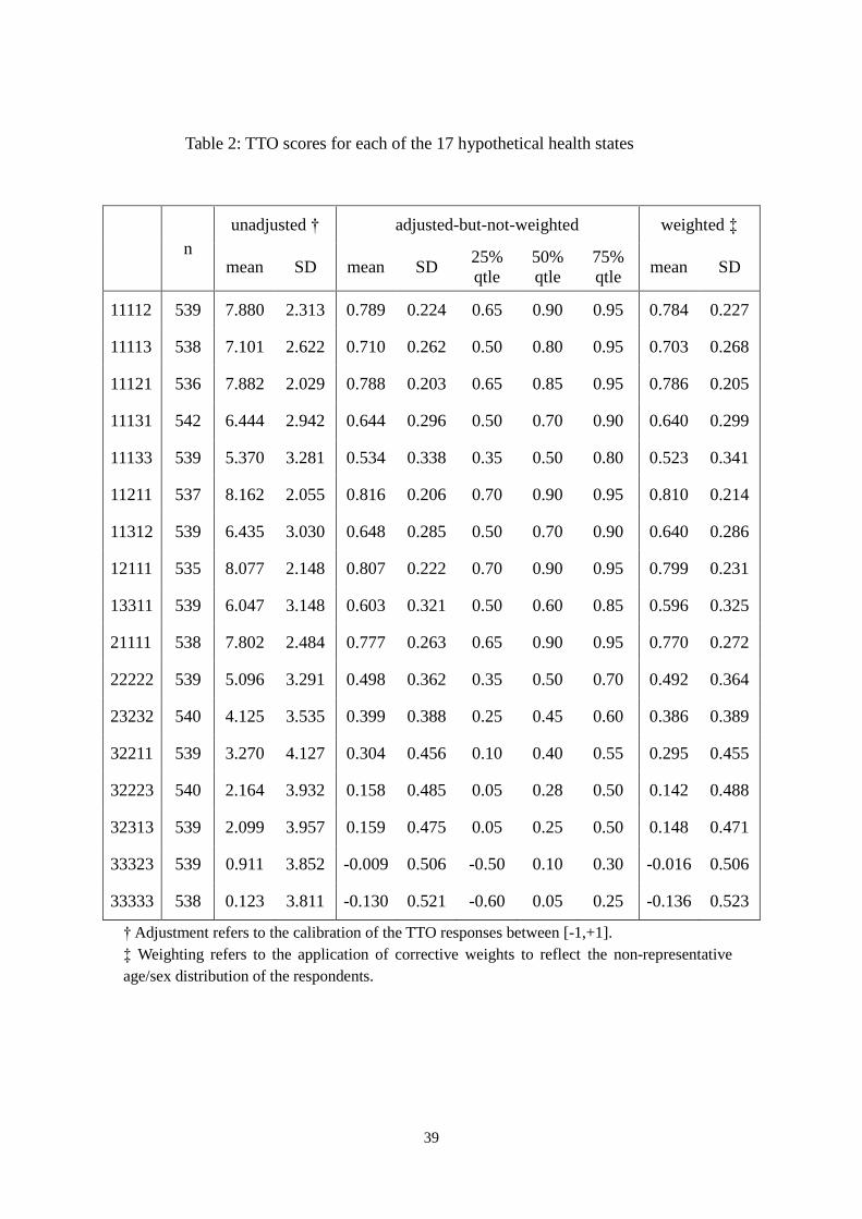
3.2 The TTO data set

Table 2 shows the unadjusted, adjusted-but-not-weighted, and

adjusted-and-weighted average TTO scores for each of the 17 hypothetical health

states. The weighted means are smaller than the non-weighted means for all 17

health states, and the difference is not large (0.008 on average).

3.2.1 Logical consistency

The present study yields 136217 C health state pairs, out of which 68 have a

logically determined relationship. 58.6% of respondents have a weak inconsistency

rate lower than 3%, and less than 10% of respondents violate more than 15% of the

time. More people violate the strong requirement so that 54.2% have an

23

inconsistency rate higher than 15%, while those that violate the requirement for more

than half the time are less than 10% of all respondents.

An analysis of scatter-plots indicates that violations are correlated to the distance

between health states, and further, for health state pairs with larger distance scores, the

difference between the weak and strong consistencies are much smaller indicating that

most of the strong inconsistency occurs with pairs with smaller distance.

Therefore the inconsistencies as a whole are due to measurement or perception error,

rather than to failure to understand the valuation task. Further, none of the 68 health

state pairs are inconsistent at the aggregate level.

3.2.2 Inter-respondent correlation

Spearman’s rank order correlation coefficient () between the TTO responses of

each respondent and the average TTO indicates that there is high consistency of TTO

rankings across individual respondents. The mean value of is 0.774 and the median

is 0.831, while the minimum value of to reject the null hypothesis (that there is no

rank order correlation) at a 1% significance level (2-sided) is 0.618 for n = 17. 14.2%

of respondents had a value of that is significant at this level, and 7.2% at the 5%

significance level. This indicates that, while the observed TTO values demonstrate a

fairly large variance, most respondents are in good agreement regarding the ranking of

24

the 17 health states.

3.3 Comparison with the British study

3.3.1 The TTO results

Figure 2 is a scatter-plot comparing the weighted mean adjusted TTO score of the 17

states obtained in the present study and the corresponding results from the MVH study

in Britain. This shows that, firstly, there is a high positive correlation between the

two data sets (Pearson’s correlation coefficient r = 0.924). However, secondly, there

is a systematic bias such that the Japanese observed values are consistently higher than

the British observed values except for the very mild states. In absolute terms, the

mean difference is 0.241 and the maximum difference is 0.585 (state 11133).

There is a similar relationship between the observed Japanese values and the

predicted values under the British tariff for the 17 health states (cf. Table 5). MAE is

0.228 and the maximum error is 0.527 (state 23232). Note that, on a scale between

–1 and 1, these figures are unacceptably large. To compare, MAE in the British

context is 0.039 with maximum error of 0.120.

This poor match and the systematic bias justify the creation of a special EQ-5D

value set for Japan.

25

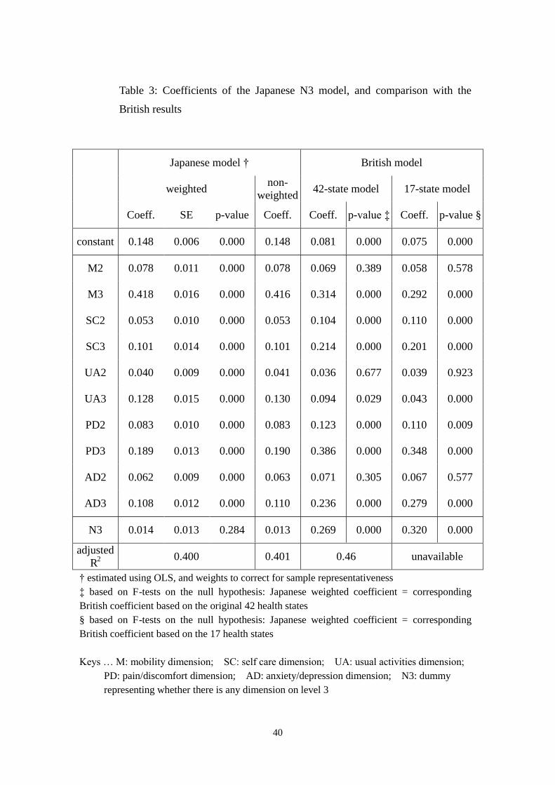
3.3.2 The Japanese N3 value set

Table 3 illustrates the result of the Japanese N3 estimation with and without

corrective weights. All the coefficients have p < 0.001, except for N3, and the

expected signs. Presence of heteroscedasticity is indicated (RESET test, p < 0.001),

and the reported p values are based on robust standard errors, correcting for this.

Coefficients of the British value set are reproduced for comparison, in the 6th

column. The 7th column shows the p-values from F-tests for the null hypothesis: that

the Japanese weighted coefficient is equal to the corresponding British coefficient.

Eight out of the twelve coefficients are markedly different (p < 0.001). The 8th and

9th columns are for the coefficients estimated using a subset of the MVH data where

valuation is limited to those of the 17 health states used in this study[9]. This time,

nine out of the twelve are different. There is a clear pattern in both cases such that the

direction of the difference is always the same within a given dimension, and therefore

it can be inferred that that the Japanese, compared to the British, are:

affected more, by having:

any diversion from full health (i.e. the constant term),

problems in the mobility dimension,

problems in the usual activity dimension, and

affected less, by having:

any extreme problem (i.e. the N3 term)

problems in the self-care dimension,

problems in the pain/discomfort dimension, and

26

problems in the anxiety/depression dimension.

3.4 Alternative models

Table 4 demonstrates the results of four models that did better than the others in

terms of goodness of fit. As can be seen, while there are no improvements in terms of

R2 across different models, the plain main effects model demonstrates improvement in

terms of p-values. None of the alternative models remove heteroscedasticity (p <

0.001). The models without the intercept demonstrated a systematic bias such that

the predicted values of the mild states are higher, and therefore are not reported.

Table 5 reports the goodness of fit of these four models. For each of the 17 health

states the error in predicting the values observed in the TTO exercise is shown. The

corresponding error using the British value set is also presented, and it is clear that

there is substantial improvement in goodness of fit by using local models. The

correlation between the observed and the predicted is at least 0.998, and there are no

systematic biases. Figure 3 illustrates the case of the plain main effects model.

When the respondents are split randomly into two groups of equal size, and the

observed values of one group are predicted based on the value set formed from the

observation of the other group, and vice versa, the two sets of values are highly

correlated under all four models (r = 0.996 to r = 0.998). MAE ranges from 0.023 to

27

0.027. This narrowness demonstrates the robustness of the models.

In short, the four models perform almost equally well. However, there are two

reasons to favour the plain main effects model over the remaining three models: firstly,

all coefficients are highly significant, and secondly, it has the fewest variables and thus

is the simplest.

4 . D i s c u s s i o n

Several things can be inferred from this study, the most important of them being

that:

(1) the health related preferences of the British and the Japanese public differ

systematically with regards to the 5 dimensions of EQ-5D, and

(2) a local value set with very high goodness of fit is estimated, from 17 EQ-5D

health states using fairly simple estimation techniques.

Each of these is discussed below in turn.

Regarding the first point, different observations between the British study and the

present study can be caused by four possible factors:

(a) differences in peoples’ health related preferences,

(b) noise introduced during the translation process of the descriptive instrument

(EQ-5D),

28

(c) noise introduced during the translation of the valuation procedure (TTO

manual), and

(d) differences in the design and methods of the two studies.

It is the first of these that we want to single out. Of the four factors, (c) and (d) are

unlikely to be the main source of the differences because the observed differences

listed in section 3.3.2. occur in both directions, and health attributes would not be

selectively affected by these two factors. Factor (b) is more troublesome because no

matter how carefully or meticulously the translation process is undertaken, problems

will continue to remain, as has been observed in the translation of SF-36 into Japanese

[16]. To further complicate things, factors (a) and (b) are interrelated. On the one

hand, to rule out factor (b) and to establish that two different language versions have

the same conceptual equivalence, we need to assume factor (a) is absent and that the

concept of health and its valuation are largely shared across languages and cultures.

On the other hand, in order to examine factor (a), we need to assume that factor (b) is

absent (the absence of which is examined by assuming that factor (a) is cleared).

Thus, the relationship between factors (a) and (b) cannot be determined within one

study. In this respect, further comparative valuation studies that alter either the

descriptive instrument or the valuation procedure (but not both), will be of much value.

However, what is crucial is that this relationship does not lead to an argument against

the estimation and the use of local value sets. By employing the local value set, both

29

the difference in health related preferences and the noise from the translation process

of the instrument have been simultaneously and effectively removed.

The effect of the systematic difference observed is that, for example, a treatment that

cured problems in self care, pain, and depression with side effects involving mobility,

and usual activities (eg. a change from 11333 to 22222) is likely to be appreciated less

by an average Japanese than a British. Obviously, the effectiveness of an intervention

is not a simple function of the descriptive changes in health outcomes, but also on how

these are valued.

Regarding the second point, of the studies that use TTO as the valuation method to

estimate population value sets for EQ-5D, the MVH study is of the largest scale to date,

both in terms of the number of respondents and the number of health states valued.

This latter factor has been a serious constraint for reproducing the study both within

the UK and elsewhere. However, the present study has demonstrated the encouraging

fact that it is possible to estimate a value set with comparable goodness of fit from a

much smaller number of states.

There are two associated elements: (i) that the modified protocol can be as efficient

as the original, and (ii) that the plain main effects model has been sufficient to estimate

a value set with good fit. Of these two, the former is relatively more likely to hold

across different environments and cultures than the latter. The main reason for the

30

plain main effects model outperforming the N3 model in modelling the Japanese data

is because the observed TTO values in the present study are distributed differently

from the British values. When the plain main effects model is applied to the MVH

dataset, a clear bias is observed so that the predicted values of the more severe states

are larger than the observed states, and this is why the N3 model, which gives

additional weight to extreme problems, works. However, there is no such bias with

the Japanese data, as is indicated by the p-value of the N3 coefficient in this model.

This indicates that the particular model specification is likely to differ across

populations and cultures.

5 . C o n c l u s i o n

This study elicits preferences of the Japanese public regarding hypothetical EQ-5D

health states using the “modified” MVH protocol. Since the MAE of predicting the

observed Japanese values using the British value set is 0.228 with maximum error of

0.527, and with bias over severity, we conclude that Japan should develop its own

social value set. The plain main effects model produces a value set with good fit, a

MAE of 0.015, maximum error of 0.031, and without biases. Thus, the local

Japanese value set offers a substantial improvement compared to applying the British

31

value set in this environment.

32

R e f e r e n c e s

1. Gold RM, Siegel JE, Russell LB, et al. eds. Cost-Effectiveness in Health and

Medicine: Oxford University Press; 1996.

2. Kind P, Rosser R, Williams A. Valuation of quality of life: Some psychometric

evidence. In Jones-Lee MW, ed. The Value of Life and Safety: North-Holland; 1982.

3. Dolan P. Modeling valuations for EuroQol health states. Medical Care.

1997;35:1095-1108.

4. Torrance GW, Furlong W, Feeny D, et al. Multi-attribute preference functions:

Health Utilities Index. PharmacoEconomics. 1995;7:503-520.

5. Dolan P, Gudex C, Kind P, et al. A Social Tariff for EuroQol: Results from a UK

General Population Survey. Centre for Health Economics, University of York,

Discussion Paper 138; 1995

6. Williams A. The Measurement and Valuation of Health: A Chronicle. Centre for

Health Economics, University of York, Discussion Paper 136; 1995

7. Brooks R, the EuroQol Group. EuroQol: The current state of play. Health Policy.

1996;37:53-72.

8. Gudex C. Time Trade-Off User Manual: Props and Self-Completion Methods.:

Centre for Health Economics, University of York; 1994.

33

9. Macran S, Kind P. Valuing EQ-5D health states using a modified MVH protocol:

Preliminary results. in Badia X, Herdman M, Roset M eds. Proceedings of the 16th

Plenary Meeting of the EuroQol Group, Sitges, 2000

10. The Japanese EuroQol Translation Team. The development of the Japanese

EuroQol Instrument (in Japanese). Journal of Health Care and Society.

1998;8:109-124.

11. The Japanese EuroQol Translation Team. The Japanese EuroQol Instrument.

unpublished report to the EuroQol Translation Committee, 1997

12. Ikeda S, Ikegami N, on behalf of the Japanese EuroQol Tariff Project. Health status

in Japanese Population: Results from Japanese EuroQol study (in Japanese).

Journal of Health Care and Society. 1999;9:83-92.

13. Ikeda S, Sakai I, Tamura M, et al. VAS valuations of hypothetical health states

using EQ-5D in Japan. paper presented at the EuroQol Group Meeting. Pampolna;

2000.

14. Patrick DL, Starks HE, Cain KC, et al. Measuring preferences for health states

worse than death. Medical Decision Making. 1994:9-18.

15. Brazier J, Usherwood T, Harper R, et al. Deriving a preference-based single index

from the UK SF-36 health survey. Journal of Clinical Epidemiology.

1998;51:1115-1128.

34

16. Fukuhara S, Bito S, Green J, et al. Translation, adaptation, and validation of the

SF-36 Health Survey for use in Japan. Journal of Clinical Epidemiology.

1998;51:1037-1044.

35

F i g u r e s

Figure 1: the EQ-5D 5-dimensional descriptive system

Mobility No problems in walking about Some problems in walking about Confined to bed

Self-Care

No problems with self-care Some problems washing or dressing oneself Unable to wash or dress oneself

Usual Activities (e.g. work, study, housework, family or leisure activities)

No problems with performing one’s usual activities Some problems with performing one’s usual activities Unable to perform one’s usual activities

Pain/Discomfort

No pain or discomfort Moderate pain or discomfort Extreme pain or discomfort

Anxiety/Depression

Not anxious or depressed Moderately anxious or depressed Extremely anxious or depressed

A statement with no problems is referred to as level 1, and a statement with inability or extreme problem is referred to as level 3, so that for example, health state 21232 means:

some problems in walking about, no problems washing and dressing oneself, some problems with performing one’s usual activities, extreme pain or discomfort, and moderately anxious or depressed.

This 5-dimension descriptive system can identify 35=243 different health states.

36

Figure 2: Comparing the mean adjusted TTO values in Japan with those

obtained in the UK study

Figure 2: Comparing the mean adjusted TTO values in Japan

with those obtained in the UK study

-0.6

-0.4

-0.2

0.0

0.2

0.4

0.6

0.8

1.0

-0.2 0.0 0.2 0.4 0.6 0.8 1.0

observed values of the Japanese study

observ

ed v

alu

es o

f th

e M

VH

stu

dy

37

Figure 3: Comparing the observed values and values predicted from the plain

main effects model

Figure 3: Comparing the observed values and

values predicted from the plain main effects model

-0.2

0.0

0.2

0.4

0.6

0.8

1.0

-0.2 0.0 0.2 0.4 0.6 0.8 1.0

observed values of the Japanese study

pre

dic

ted v

alues

of th

e pla

in m

ain e

ffec

tes

model

38

Ta b l e s

Table 1: A comparison of the background characteristics of those included in

and those excluded from the analysis

of those included

of those excluded

p-value (2-sided)

have experienced serious illness in themselves 0.147 0.221 0.097

have experienced serious illness in the family 0.346 0.377 0.601

have experienced serious illness in others 0.328 0.273 0.333

females 0.424 0.442 0.765

current smokers 0.357 0.325 0.575

main activity is “in employment or self employment” 0.501 0.442 0.330

main activity is “housework” 0.390 0.295 0.108

continued education beyond minimum schooling 0.788 0.623 0.001

have Degree or equivalent professional qualification 0.333 0.247 0.128

39

Table 2: TTO scores for each of the 17 hypothetical health states

n unadjusted † adjusted-but-not-weighted weighted ‡

mean SD mean SD 25% qtle

50% qtle

75% qtle

mean SD

11112 539 7.880 2.313 0.789 0.224 0.65 0.90 0.95 0.784 0.227

11113 538 7.101 2.622 0.710 0.262 0.50 0.80 0.95 0.703 0.268

11121 536 7.882 2.029 0.788 0.203 0.65 0.85 0.95 0.786 0.205

11131 542 6.444 2.942 0.644 0.296 0.50 0.70 0.90 0.640 0.299

11133 539 5.370 3.281 0.534 0.338 0.35 0.50 0.80 0.523 0.341

11211 537 8.162 2.055 0.816 0.206 0.70 0.90 0.95 0.810 0.214

11312 539 6.435 3.030 0.648 0.285 0.50 0.70 0.90 0.640 0.286

12111 535 8.077 2.148 0.807 0.222 0.70 0.90 0.95 0.799 0.231

13311 539 6.047 3.148 0.603 0.321 0.50 0.60 0.85 0.596 0.325

21111 538 7.802 2.484 0.777 0.263 0.65 0.90 0.95 0.770 0.272

22222 539 5.096 3.291 0.498 0.362 0.35 0.50 0.70 0.492 0.364

23232 540 4.125 3.535 0.399 0.388 0.25 0.45 0.60 0.386 0.389

32211 539 3.270 4.127 0.304 0.456 0.10 0.40 0.55 0.295 0.455

32223 540 2.164 3.932 0.158 0.485 0.05 0.28 0.50 0.142 0.488

32313 539 2.099 3.957 0.159 0.475 0.05 0.25 0.50 0.148 0.471

33323 539 0.911 3.852 -0.009 0.506 -0.50 0.10 0.30 -0.016 0.506

33333 538 0.123 3.811 -0.130 0.521 -0.60 0.05 0.25 -0.136 0.523

† Adjustment refers to the calibration of the TTO responses between [-1,+1]. ‡ Weighting refers to the application of corrective weights to reflect the non-representative age/sex distribution of the respondents.

40

Table 3: Coefficients of the Japanese N3 model, and comparison with the

British results

Japanese model † British model

weighted non-

weighted 42-state model 17-state model

Coeff. SE p-value Coeff. Coeff. p-value ‡ Coeff. p-value §

constant 0.148 0.006 0.000 0.148 0.081 0.000 0.075 0.000

M2 0.078 0.011 0.000 0.078 0.069 0.389 0.058 0.578

M3 0.418 0.016 0.000 0.416 0.314 0.000 0.292 0.000

SC2 0.053 0.010 0.000 0.053 0.104 0.000 0.110 0.000

SC3 0.101 0.014 0.000 0.101 0.214 0.000 0.201 0.000

UA2 0.040 0.009 0.000 0.041 0.036 0.677 0.039 0.923

UA3 0.128 0.015 0.000 0.130 0.094 0.029 0.043 0.000

PD2 0.083 0.010 0.000 0.083 0.123 0.000 0.110 0.009

PD3 0.189 0.013 0.000 0.190 0.386 0.000 0.348 0.000

AD2 0.062 0.009 0.000 0.063 0.071 0.305 0.067 0.577

AD3 0.108 0.012 0.000 0.110 0.236 0.000 0.279 0.000

N3 0.014 0.013 0.284 0.013 0.269 0.000 0.320 0.000

adjusted R2

0.400 0.401 0.46 unavailable

† estimated using OLS, and weights to correct for sample representativeness ‡ based on F-tests on the null hypothesis: Japanese weighted coefficient = corresponding British coefficient based on the original 42 health states § based on F-tests on the null hypothesis: Japanese weighted coefficient = corresponding British coefficient based on the 17 health states Keys … M: mobility dimension; SC: self care dimension; UA: usual activities dimension;

PD: pain/discomfort dimension; AD: anxiety/depression dimension; N3: dummy representing whether there is any dimension on level 3

41

Table 4: Alternative models for Japan † ‡

plain N3 C3sq N3 + C3sq

coeff. p-values coeff. p-values coeff. p-values coeff. p-values

constant 0.152 0.000 0.148 0.000 0.153 0.000 0.141 0.000

M2 0.075 0.000 0.078 0.000 0.073 0.000 0.083 0.000

M3 0.418 0.000 0.418 0.000 0.409 0.000 0.330 0.000

SC2 0.054 0.000 0.053 0.000 0.055 0.000 0.067 0.000

SC3 0.102 0.000 0.101 0.000 0.096 0.000 0.044 0.048

UA2 0.044 0.000 0.040 0.000 0.047 0.000 0.044 0.000

UA3 0.133 0.000 0.128 0.000 0.129 0.000 0.062 0.019

PD2 0.080 0.000 0.083 0.000 0.079 0.000 0.087 0.000

PD3 0.194 0.000 0.189 0.000 0.189 0.000 0.114 0.000

AD2 0.063 0.000 0.062 0.000 0.063 0.000 0.058 0.000

AD3 0.112 0.000 0.108 0.000 0.109 0.000 0.053 0.021

N3 0.014 0.284 0.087 0.000

C3sq 0.001 0.504 0.012 0.003

adjusted R2 0.400 0.400 0.400 0.401

† the p-values are based on OSL estimations: fixed and random effects estimates yield smaller p-values, while the coefficients are insensitive. ‡ the figures are based on regressions with population corrective weights. Keys … M: mobility dimension; SC: self care dimension; UA: usual activities dimension;

PD: pain/discomfort dimension; AD: anxiety/depression dimension; N3: dummy representing whether there is any dimension on level 3; C3sq: the square of the number of dimensions with level 3

42

Table 5: Difference between the 17 observed values and the values predicted

by the four models †

5D state Japanese value set

British value set

plain N3 C3sq N3+C3sq N3

11112 0.004 0.000 0.006 -0.011 -0.058

11113 -0.024 -0.019 -0.024 0.005 0.298

11121 0.020 0.019 0.020 0.015 -0.008

11131 -0.012 -0.007 -0.014 -0.003 0.379

11133 -0.006 -0.006 -0.008 -0.022 0.508

11211 0.011 0.003 0.016 0.000 -0.067

11312 0.001 0.005 0.000 0.014 0.168

12111 0.009 0.005 0.012 0.011 -0.011

13311 -0.006 -0.002 -0.009 -0.010 0.266

21111 0.002 0.002 0.002 0.000 -0.074

22222 -0.030 -0.033 -0.027 -0.018 -0.013

23232 0.030 0.033 0.027 0.021 0.527

32211 -0.030 -0.025 -0.032 -0.017 0.106

32223 0.022 0.024 0.019 0.017 0.324

32313 0.031 0.030 0.029 0.008 0.260

33323 -0.007 -0.006 -0.008 -0.010 0.327

33333 -0.007 -0.014 0.000 0.010 0.476

MAE ‡ 0.015 0.014 0.015 0.011 0.228

† The positive (negative) sign indicates that the predicted value is smaller (larger) than the observed value ‡ MAE: mean absolute error.