Estimating Attendance From Cellular Network Data

Marco MameiDipartimento di Scienze e Metodi dell’Ingegneria

University of Modena and Reggio Emilia, Italymarco.mamei@unimore.it

Massimo ColonnaEngineering & TilabTelecom Italia, Italy

massimo.colonna @telecomitalia.it

ABSTRACTWe present a methodology to estimate the number of atten-dees to events happening in the city from cellular networkdata. In this work we used anonymized Call Detail Records(CDRs) comprising data on where and when users access thecellular network. Our approach is based on two key ideas:(1) we identify the network cells associated to the event loca-tion. (2) We verify the attendance of each user, as a measureof whether (s)he generates CDRs during the event, but notduring other times. We evaluate our approach to estimatethe number of attendees to a number of events ranging fromfootball matches in stadiums to concerts and festivals in opensquares. Comparing our results with the best groundtruthdata available, our estimates provide a median error of lessthan 15% of the actual number of attendees.

Categories and Subject DescriptorsG.3 [Probability and statistics]: Time series analy-sis; H.3.3 [Information Search and Retrieval]: Re-trieval Models; I.5.2 [Design Methodology]: PatternAnalysis

General TermsCDR, attendance estimation, mobility patterns

1. INTRODUCTIONThe widespread diffusion of mobile phones and cell

networks provides a practical way to collect geo-locatedinformation from a large user population. The analy-sis of such collected data is a fundamental asset in thedevelopment of pervasive and mobile computing appli-cations, including location-based services, traffic man-agement, urban planning, and disaster response [1, 2,3, 4, 5, 6, 7].

In this work, we explore the use of anonymized CallDetail Records (CDRs) from a cellular network to esti-mate the number of attendees to large events happeningin the city.

Each CDR contains information such as the time amobile phone accesses the network (e.g., to send/receivecalls and text messages), as well as the identity of the

cell tower with which the phone was associated at thattime. CDRs can serve as sporadic samples of the ap-proximate locations of the phone’s owner.

On the basis of such location samples, we try to un-derstand if a user was attending a given event and es-timate the number of attendees on that basis.

While in some contexts, the number of participantscan be deducted also by other means (e.g., ticketing in-formation), there are many scenarios in which countingthe attendance is problematic (e.g., events held in opensquares, parades, flash-mobs) and an estimate on thebasis of cellular network data is highly valuable.

Estimating events’ attendance has a number of prac-tical and useful applications.

On the one hand, it is an important information forthe local government and organizers in that it is at thebasis of event’s planning and resource prioritization. Inaddition, since CDRs allow to track the movements ofindividual users, it is possible to understand where at-tendees come from and where they go after the event.This naturally supports traffic and road management.

On the other hand, such kind of information, can sup-port advertisement systems [8] by providing accurateaudience measurements. Also in this case, the possibil-ity of tracking users would open to advanced applica-tions for the provisioning of highly personalized adver-tising and marketing schemas. Despite users’ hashedids do not allow to identify the real person behind aphone, this opens a number of privacy concerns. Whilesome research addressing such concerns exist [9, 10], wewill not tackle privacy problems in this paper focusingon the attendance estimation problem only.

While a number of existing works deal with the prob-lem of discovering and analyzing events on the basis ofcellular network data (see Related Work section), theproblem of actually estimating the number of attendeesis largely unexplored. In particular, to the best of ourknowledge, there are not published results of the accu-racy of attendance estimation using CDRs.

The goal of this paper is to present such an estima-tion procedure. In particular, in Section 2 we presenta naive approach to estimate the attendance and illus-

1

arX

iv:1

504.

0738

5v1

[cs

.SI]

28

Apr

201

5

trate why it does not work properly. In Section 3 wepresent our methodology. In Section 4, we evaluate ourapproach to estimate the number of attendees to foot-ball matches in stadiums, in which reliable groundtruthdata were available. Section 5 discusses how to improveperformance on the basis of the knowledge of multi-ple events in the area. Section 6 presents related work.Eventually, Section 7 concludes and discuss some futureavenues for improvement.

2. NAIVE APPROACHBefore illustrating the proposed methodology, we want

to show the main problem that complicates the task ofestimating the number of attendees.

A naive approach to address such an issue would beto just count the number of users who generate CDRsin cells covering the event’s location area during theevent time. In particular, we tried to apply the naiveapproach to estimate the number of attendees to foot-ball matches in two different stadiums in Turin, Italy.We defined the area associated to each stadium as a cir-cle centered in the stadium with a fixed radius of 100m.Then, we record all the CDRs produced in the networkcells that overlap with the stadiums’ area at the eventtime. We then counted the number of individual users.

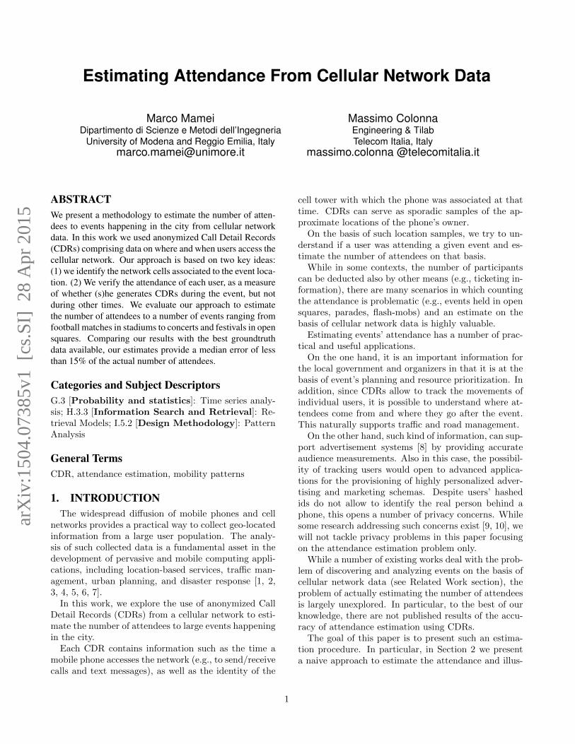
Figure 1 illustrates the result. The graphs repre-sent the hourly count of users in the area associatedwith the stadiums (Stadio Olimpico on the left, Juven-tus Stadium on the right). We also highlighted foot-ball matches taking place in the stadiums with alsogroundtruth estimates for the number of attendees.

It is rather easy to see that the naive approach ishighly ineffective. For example, the match that hap-pened on March 12, 2012 at the Stadio Olimpico is re-ported to have 21453 attendees and a CDR users’ countwith a peak of about 3700. In contrast, the match thathappened on March 20, 2012 at the Juventus Stadium isreported to have a double number of attendees (40045),while a CDR users’ peak of about one-sixth (600).

The problem with these numbers is not in the dis-crepancy between groundtruth and CDR counts. Thiscan be naturally explained by the fact that not all theusers use the phone during the match, and by the factthat not all of them adopts the same carrier providingthe data for this analysis.

The problem is in the negative correlation betweengroundtruth and CDR counts: large events (happeningat the Juventus Stadium) appear to be smaller than“small” ones (happening at the Stadio Olimpico).

The reason for such a negative correlation can be eas-ily found in the geography of the city. Stadio Olimpicois right in the city center. Juventus Stadium is in thesuburbs. Accordingly, while network cells around Ju-ventus Stadium are likely to measure CDRs comingfrom the stadium itself, network cells around Stadio

0

100

200

300

400

500

600

700

0

500

1000

1500

2000

2500

3000

3500

4000

N. U

se

rs

Juventus Stadium, TurinStadio Olimpico, Turin

Mon, 12/3/2012 Sun, 18/3/2012 Tue, 20/3/2012 Sun, 25/3/2012

Groundtruth attendance = 21453

Groundtruth attendance = 40045

Groundtruth attendance = 38536

N. U

se

rs

Figure 1: Hourly count of users generatingCDRs in the area associated with the stadiums(Stadio Olimpico on the left, Juventus Stadiumon the right). The problem is in the nega-tive correlation between groundtruth and CDRcounts: large events appear to be smaller than“small” ones.

●●

●

●

●

●

●

●●

●

●

●●●

●

●●

●

●

●

●

●

●●

●

●●●●

●

10000

20000

30000

40000

1000 2000 3000 4000CDR Estimate

Gro

undt

ruth

●●

●●●●

●●

JuventusStadiumTO

ParcoDoraTO

PiazzaSanCarloTO

PiazzaVittorioTO

PiazzaCastelloTO

StadioOlimpicoTO

StadioSilvioPiolaNO

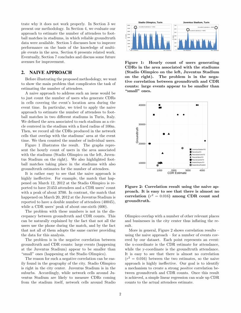
Figure 2: Correlation result using the naive ap-proach. It is easy to see that there is almost nocorrelation (r2 = 0.016) among CDR count andgroundtruth.

Olimpico overlap with a number of other relevant placesand businesses in the city center thus inflating the re-sult.

More in general, Figure 2 shows correlation results –using the naive approach – for a number of events cov-ered by our dataset. Each point represents an event:the x-coordinate is the CDR estimate for attendance,while the y-coordinate is the groundtruth attendance.It is easy to see that there is almost no correlation(r2 = 0.016) between the two estimates, so the naiveapproach is highly ineffective. Our goal is to identifya mechanism to create a strong positive correlation be-tween groundtruth and CDR counts. Once this resultis achieved, a simple linear regression can scale up CDRcounts to the actual attendees estimate.

2

1)

Event Place

CDR Event2) Best Radius

3)

Attendees

4)

Scaling

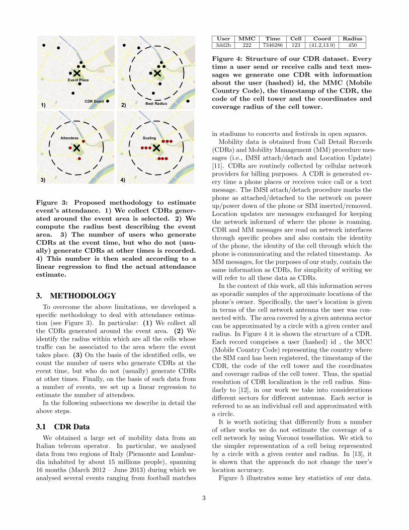
Figure 3: Proposed methodology to estimateevent’s attendance. 1) We collect CDRs gener-ated around the event area is selected. 2) Wecompute the radius best describing the eventarea. 3) The number of users who generateCDRs at the event time, but who do not (usu-ally) generate CDRs at other times is recorded.4) This number is then scaled according to alinear regression to find the actual attendanceestimate.

3. METHODOLOGYTo overcome the above limitations, we developed a

specific methodology to deal with attendance estima-tion (see Figure 3). In particular: (1) We collect allthe CDRs generated around the event area. (2) Weidentify the radius within which are all the cells whosetraffic can be associated to the area where the eventtakes place. (3) On the basis of the identified cells, wecount the number of users who generate CDRs at theevent time, but who do not (usually) generate CDRsat other times. Finally, on the basis of such data froma number of events, we set up a linear regression toestimate the number of attendees.

In the following subsections we describe in detail theabove steps.

3.1 CDR DataWe obtained a large set of mobility data from an

Italian telecom operator. In particular, we analyseddata from two regions of Italy (Piemonte and Lombar-dia inhabited by about 15 millions people), spanning16 months (March 2012 – June 2013) during which weanalysed several events ranging from football matches

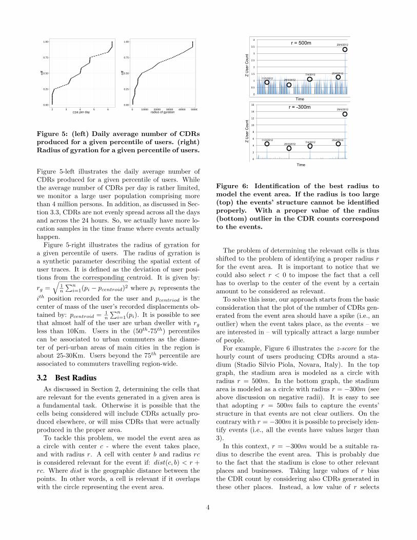
User MMC Time Cell Coord Radius3dd2b 222 7346286 123 (41.2,13.9) 450

Figure 4: Structure of our CDR dataset. Everytime a user send or receive calls and text mes-sages we generate one CDR with informationabout the user (hashed) id, the MMC (MobileCountry Code), the timestamp of the CDR, thecode of the cell tower and the coordinates andcoverage radius of the cell tower.

in stadiums to concerts and festivals in open squares.Mobility data is obtained from Call Detail Records

(CDRs) and Mobility Management (MM) procedure mes-sages (i.e., IMSI attach/detach and Location Update)[11]. CDRs are routinely collected by cellular networkproviders for billing purposes. A CDR is generated ev-ery time a phone places or receives voice call or a textmessage. The IMSI attach/detach procedure marks thephone as attached/detached to the network on powerup/power down of the phone or SIM inserted/removed.Location updates are messages exchanged for keepingthe network informed of where the phone is roaming.CDR and MM messages are read on network interfacesthrough specific probes and also contain the identityof the phone, the identity of the cell through which thephone is communicating and the related timestamp. AsMM messages, for the purposes of our study, contain thesame information as CDRs, for simplicity of writing wewill refer to all these data as CDRs.

In the context of this work, all this information servesas sporadic samples of the approximate locations of thephone’s owner. Specifically, the user’s location is givenin terms of the cell network antenna the user was con-nected with. The area covered by a given antenna sectorcan be approximated by a circle with a given center andradius. In Figure 4 it is shown the structure of a CDR.Each record comprises a user (hashed) id , the MCC(Mobile Country Code) representing the country wherethe SIM card has been registered, the timestamp of theCDR, the code of the cell tower and the coordinatesand coverage radius of the cell tower. Thus, the spatialresolution of CDR localization is the cell radius. Sim-ilarly to [12], in our work we take into considerationsdifferent sectors for different antennas. Each sector isrefereed to as an individual cell and approximated witha circle.

It is worth noticing that differently from a numberof other works we do not estimate the coverage of acell network by using Voronoi tessellation. We stick tothe simpler representation of a cell being representedby a circle with a given center and radius. In [13], itis shown that the approach do not change the user’slocation accuracy.

Figure 5 illustrates some key statistics of our data.

3

●●●●●●●●●●●●●●●●●●●●●●●●●

●●

●●

●●

●●

●●●●●●●●

●●

●●

●●

●●

●●●●●●●●●

●●

●●

●●

●●

●●●●●●●●●

●●

●●

●●

●●

●●●●●●●●●●●●●●●●●

0.00

0.25

0.50

0.75

1.00

2 3 4 5 6pls per day

cdf

CDR

●●●●●●●●●●●●●●●●●●●●●●●●●●●●●●●●●●●●●●●●●●●●●●●●●●

●●

●●

●●

●●

●●

●●

●●

●●

●●

●●

●●

●●

●●

●●

●●

●●

●●

●●

●●

●●

●●●●●●●●●●

0.00

0.25

0.50

0.75

1.00

0 10000 20000 30000 40000 50000radius of gyration

cdf

Figure 5: (left) Daily average number of CDRsproduced for a given percentile of users. (right)Radius of gyration for a given percentile of users.

Figure 5-left illustrates the daily average number ofCDRs produced for a given percentile of users. Whilethe average number of CDRs per day is rather limited,we monitor a large user population comprising morethan 4 million persons. In addition, as discussed in Sec-tion 3.3, CDRs are not evenly spread across all the daysand across the 24 hours. So, we actually have more lo-cation samples in the time frame where events actuallyhappen.

Figure 5-right illustrates the radius of gyration fora given percentile of users. The radius of gyration isa synthetic parameter describing the spatial extent ofuser traces. It is defined as the deviation of user posi-tions from the corresponding centroid. It is given by:

rg =√

1n

∑ni=1(pi − pcentroid)2 where pi represents the

ith position recorded for the user and pcentriod is thecenter of mass of the user’s recorded displacements ob-tained by: pcentroid = 1

n

∑ni=1(pi). It is possible to see

that almost half of the user are urban dweller with rgless than 10Km. Users in the (50th-75th) percentilescan be associated to urban commuters as the diame-ter of peri-urban areas of main cities in the region isabout 25-30Km. Users beyond the 75th percentile areassociated to commuters travelling region-wide.

3.2 Best RadiusAs discussed in Section 2, determining the cells that

are relevant for the events generated in a given area isa fundamental task. Otherwise it is possible that thecells being considered will include CDRs actually pro-duced elsewhere, or will miss CDRs that were actuallyproduced in the proper area.

To tackle this problem, we model the event area asa circle with center c - where the event takes place,and with radius r. A cell with center b and radius rcis considered relevant for the event if: dist(c, b) < r +rc. Where dist is the geographic distance between thepoints. In other words, a cell is relevant if it overlapswith the circle representing the event area.

0

2

4

6

8

10

12

14

16

0

0.5

1

1.5

2

2.5

3

3.5

4

11/3/2012

25/3/20127/4/2012

25/4/2012

29/4/2012

11/3/201225/3/2012

7/4/2012 25/4/2012

29/4/2012r = 500m

r = -300m

Time

Time

Z U

ser

Cou

nt

Z U

ser

Cou

nt

Figure 6: Identification of the best radius tomodel the event area. If the radius is too large(top) the events’ structure cannot be identifiedproperly. With a proper value of the radius(bottom) outlier in the CDR counts correspondto the events.

The problem of determining the relevant cells is thusshifted to the problem of identifying a proper radius rfor the event area. It is important to notice that wecould also select r < 0 to impose the fact that a cellhas to overlap to the center of the event by a certainamount to be considered as relevant.

To solve this issue, our approach starts from the basicconsideration that the plot of the number of CDRs gen-erated from the event area should have a spike (i.e., anoutlier) when the event takes place, as the events – weare interested in – will typically attract a large numberof people.

For example, Figure 6 illustrates the z-score for thehourly count of users producing CDRs around a sta-dium (Stadio Silvio Piola, Novara, Italy). In the topgraph, the stadium area is modeled as a circle withradius r = 500m. In the bottom graph, the stadiumarea is modeled as a circle with radius r = −300m (seeabove discussion on negative radii). It is easy to seethat adopting r = 500m fails to capture the events’structure in that events are not clear outliers. On thecontrary with r = −300m it is possible to precisely iden-tify events (i.e., all the events have values larger than3).

In this context, r = −300m would be a suitable ra-dius to describe the event area. This is probably dueto the fact that the stadium is close to other relevantplaces and businesses. Taking large values of r biasthe CDR count by considering also CDRs generated inthese other places. Instead, a low value of r selects

4

only relevant CDRs. It is also possible to see that theoutlier associated to the event on 29/4/2012 is readilyvisible even with r = 500m. The football match thathappened on that date, in fact, attracted almost thedouble of people (17650 persons vs. stadium’s averageof 9370). Such an event would be better represented bya larger radius (the more the people, the more the cellsnearby the stadium get saturated and rely the networkconnection to farther cells).

On the basis of the above considerations, we devel-oped an approach to identify the best radius describingthe event area. For each event happening at a loca-tion with center ec starting at time st and ending atet, we propose the the following approach. For the sakeof clarity, we present the approach in two different steps.

STEP 1.

1. For different values of r in rmin, rmax, we extractthe CDRs in the event area (cdr[]).

2. For each rk, we compute the hourly count of userswho generate CDRs in the area during the eventtime. We call xk such a count.

3. We then compute the z-score of the xk values inthe event time frame. More in detail, we computedthe hourly count of users who generate CDRs inthe area during the event time, but in i days be-fore the event (we considered 6 days before). Wethen computed the mean µk and standard devia-tion σk of this count. On this basis we computedthe z-score zk = (xk − µk)/σk. The result is a se-ries of values zk measuring how extreme the CDRcount were during the event (considering given ra-dius rk).

Data: cdr[ ], ec, st, etResult: z[ ]forall the rk ∈ [rmin, rmax] do

xk = countUsers(cdr[ ], ec, rk, st, et)forall the i ∈ [0, 6] do

yik = countUsers(cdr[ ], ec, rk, st− i ·days, et− i · days)

endµk = meani(yik) σk = sdt.devi(yik)zk = (xk − µk)/σk

end

Algorithm 1: Radius Extraction - Step 1

Algorithm 1 presents a more formal description of theapproach.

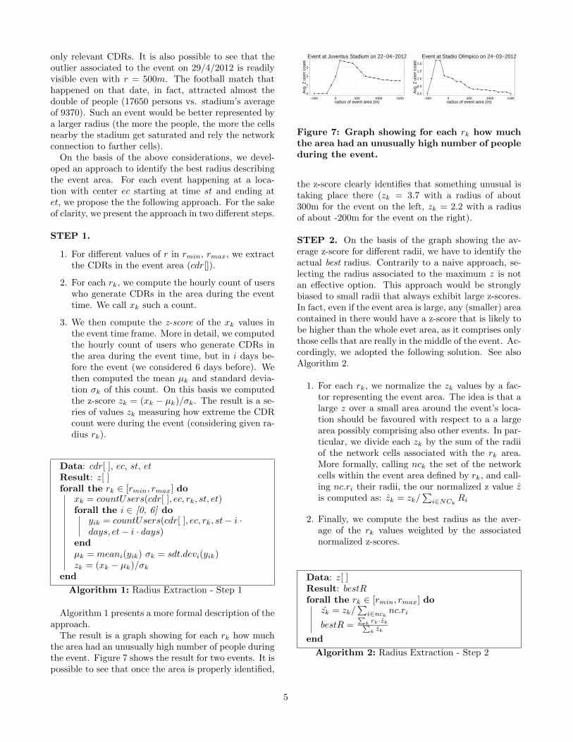
The result is a graph showing for each rk how muchthe area had an unusually high number of people duringthe event. Figure 7 shows the result for two events. It ispossible to see that once the area is properly identified,

0

1

2

3

−500 0 500 1000 1500radius of event area (m)

Avg

. Z u

ser

coun

t

Event at Juventus Stadium on 22−04−2012

0.0

0.5

1.0

1.5

2.0

−500 0 500 1000 1500radius of event area (m)

Avg

. Z u

ser

coun

t

Event at Stadio Olimpico on 24−03−2012

Figure 7: Graph showing for each rk how muchthe area had an unusually high number of peopleduring the event.

the z-score clearly identifies that something unusual istaking place there (zk = 3.7 with a radius of about300m for the event on the left, zk = 2.2 with a radiusof about -200m for the event on the right).

STEP 2. On the basis of the graph showing the av-erage z-score for different radii, we have to identify theactual best radius. Contrarily to a naive approach, se-lecting the radius associated to the maximum z is notan effective option. This approach would be stronglybiased to small radii that always exhibit large z-scores.In fact, even if the event area is large, any (smaller) areacontained in there would have a z-score that is likely tobe higher than the whole evet area, as it comprises onlythose cells that are really in the middle of the event. Ac-cordingly, we adopted the following solution. See alsoAlgorithm 2.

1. For each rk, we normalize the zk values by a fac-tor representing the event area. The idea is that alarge z over a small area around the event’s loca-tion should be favoured with respect to a a largearea possibly comprising also other events. In par-ticular, we divide each zk by the sum of the radiiof the network cells associated with the rk area.More formally, calling nck the set of the networkcells within the event area defined by rk, and call-ing nc.ri their radii, the our normalized z value zis computed as: zk = zk/

∑i∈NCk

Ri

2. Finally, we compute the best radius as the aver-age of the rk values weighted by the associatednormalized z-scores.

Data: z[ ]Result: bestRforall the rk ∈ [rmin, rmax] do

zk = zk/∑

i∈nck nc.ri

bestR =∑

k rk·zk∑k zk

end

Algorithm 2: Radius Extraction - Step 2

5

3.3 Attendance EstimatorOnce the event area has been identified, we need a

mechanism to count precisely the number of users whoattended the event. Since we do not know what the userwas doing in the event area, we estimate the probabilityof the user presence as proportional to the fraction oftime in which the user was there during the event, andinversely proportional to the fraction of time in whichthe user was there outside of the event time [14]. Thislatter point is important to eliminate users that live orwork in the event area and so are in there independentlyof the event.

As a first step, we tried to characterize the individualcalling activity and verified that it is frequent enough toallow monitoring the users’ location with a fine enoughresolution. For each user, we measured the inter-CDRtime - i.e., the time interval between two consecutivenetwork connections (similar to what has been donein [15, 1]). Focusing on a given event (e.g., a footballgame held at the Juventus Stadium in Turin on March20 2012), we performed some measures. The averageinter-CDR time measured for the population of possibleattendees (users who generate at least one CDR in theevent area during the event time) was 241 minutes. Thisnumber is large because it considers the whole dailylives of that users, thus also spanning night gaps. Wealso measured the average inter-CDR time consideringonly CDRs generated during at the event time. Withthat assumption the average inter-CDR time reduces to52 minutes.

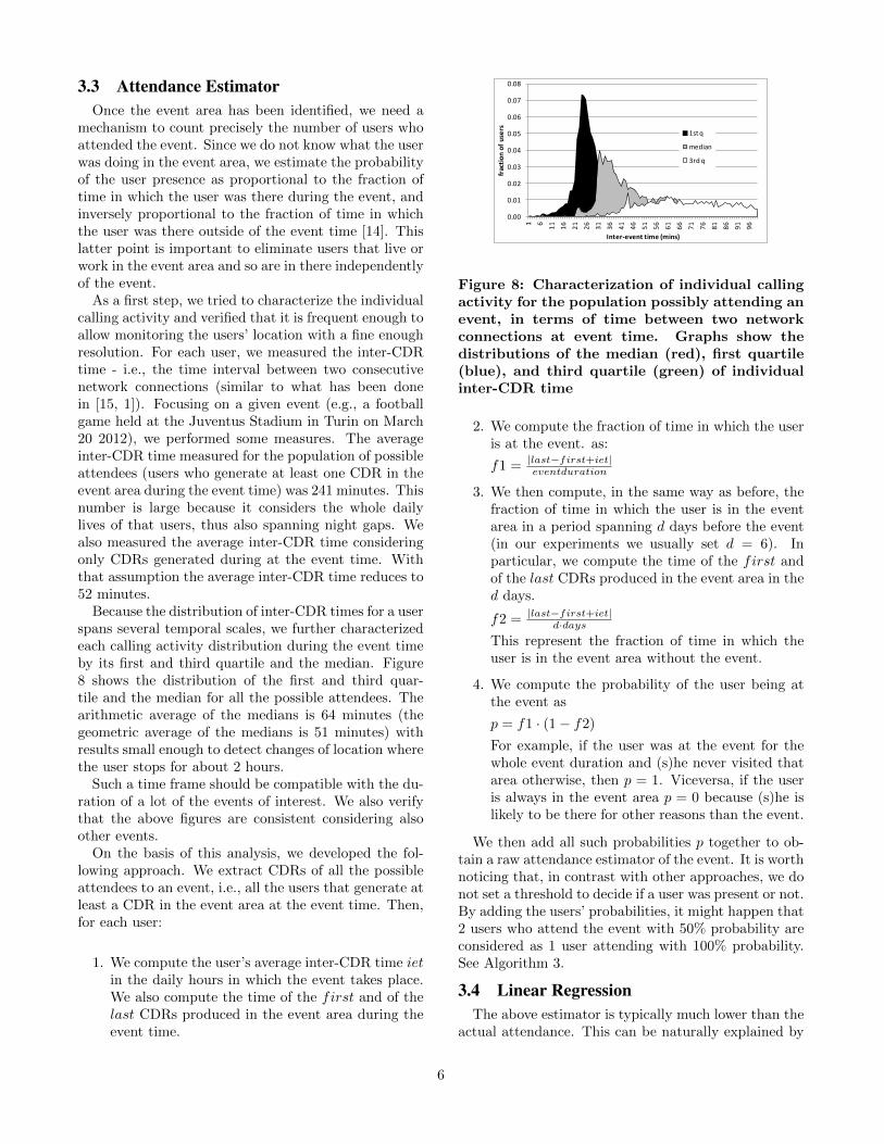
Because the distribution of inter-CDR times for a userspans several temporal scales, we further characterizedeach calling activity distribution during the event timeby its first and third quartile and the median. Figure8 shows the distribution of the first and third quar-tile and the median for all the possible attendees. Thearithmetic average of the medians is 64 minutes (thegeometric average of the medians is 51 minutes) withresults small enough to detect changes of location wherethe user stops for about 2 hours.

Such a time frame should be compatible with the du-ration of a lot of the events of interest. We also verifythat the above figures are consistent considering alsoother events.

On the basis of this analysis, we developed the fol-lowing approach. We extract CDRs of all the possibleattendees to an event, i.e., all the users that generate atleast a CDR in the event area at the event time. Then,for each user:

1. We compute the user’s average inter-CDR time ietin the daily hours in which the event takes place.We also compute the time of the first and of thelast CDRs produced in the event area during theevent time.

0.00

0.01

0.02

0.03

0.04

0.05

0.06

0.07

0.08

1 6

11

16

21

26

31

36

41

46

51

56

61

66

71

76

81

86

91

96

frac

tio

n o

f u

sers

Inter-event time (mins)

1st q

median

3rd q

Figure 8: Characterization of individual callingactivity for the population possibly attending anevent, in terms of time between two networkconnections at event time. Graphs show thedistributions of the median (red), first quartile(blue), and third quartile (green) of individualinter-CDR time

2. We compute the fraction of time in which the useris at the event. as:

f1 = |last−first+iet|eventduration

3. We then compute, in the same way as before, thefraction of time in which the user is in the eventarea in a period spanning d days before the event(in our experiments we usually set d = 6). Inparticular, we compute the time of the first andof the last CDRs produced in the event area in thed days.

f2 = |last−first+iet|d·days

This represent the fraction of time in which theuser is in the event area without the event.

4. We compute the probability of the user being atthe event as

p = f1 · (1− f2)

For example, if the user was at the event for thewhole event duration and (s)he never visited thatarea otherwise, then p = 1. Viceversa, if the useris always in the event area p = 0 because (s)he islikely to be there for other reasons than the event.

We then add all such probabilities p together to ob-tain a raw attendance estimator of the event. It is worthnoticing that, in contrast with other approaches, we donot set a threshold to decide if a user was present or not.By adding the users’ probabilities, it might happen that2 users who attend the event with 50% probability areconsidered as 1 user attending with 100% probability.See Algorithm 3.

3.4 Linear RegressionThe above estimator is typically much lower than the

actual attendance. This can be naturally explained by

6

Data: cdr[ ], bestR, ec, st, et, d = 6Result: attendancecandidates[] = usersIn(ec, bestR, st, et)forall the ci ∈ candidates do

iet = avg − inter − CDR− time(ci, cdr)first = timeFirstCDR(ec, bestR, st, et)last = timeLastCDR(ec, bestR, st, et)

f1 = |last−first+iet|eventduration

first = timeFirstCDR(ec, bestR, st−ddays, et)last = timeLastCDR(ec, bestR, st− ddays, et)f2 = |last−first+iet|

ddays

pi = f1 · (1− f2)endattendance =

∑i pi

Algorithm 3: Attendance estimator

the fact that not all the users will use the phone duringthe event, and by the fact that not all of them adoptsthe same carrier providing the data for this analysis.In any case, as we will show in the next section, ithas a strong positive correlation with groundtruth head-counts. Accordingly, a simple linear regression can scaleup the above count to the actual attendees estimate.

Rather than more complex regression algorithms, weapplied linear regression for two main reasons:

1. The goal of this work is to show that events’ at-tendance can be measured by CDRs coming fromthe cellular network. If this is true, then an esti-mator based on CDR needs only to be scaled upto provide good results. More complex regressionalgorithms could hide shortcomings of the CDRestimator that we want instead to analyze.

2. The number of events for which we have groundtruthinformation is limited. Accordingly there is a no-table risk of overfitting. Regression mechanismsmore complex than linear regression would be evenmore susceptible to this problem.

More in detail, we assume the availability of a trainingset of events to be used to fit the parameters of the linearregression. The resulting coefficients are then used toscale CDR estimates of attendance in a testing set ofevents. The combination of all the above steps producesthe final estimate of the number of attendees. In thenext section, we conduce some experiments to assessthe performance of our approach.

4. ANALYSIS AND RESULTSAs already introduced, to test the performance of

the presented methodology we try to estimate the num-ber of attendees to several events ranging from footballmatches in stadiums to concerts and festivals in opensquares. The analysis spans large events with ground

−250

0

250

500

1 2 3 4 5 6 7 8 9 10 11Event Location

Rad

ius

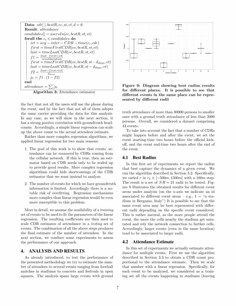
Figure 9: Diagram showing best radius resultsfor different places. It is possible to see thatdifferent events in the same place can be repre-sented by different radii

truth attendance of more than 80000 persons to smallerones with a ground truth attendance of less than 2000persons. Overall, we considered a dataset comprising43 events.

To take into account the fact that a number of CDRsmight happen before and after the event, we set theevent starting-time two hours before the official kick-off, and the event end-time two hours after the end ofthe event.

4.1 Best RadiusIn this first set of experiments we report the radius

that best capture the dynamics of a given event. Werun the algorithm described in Section 3.2. Specifically,we varied r in rk ∈ [−500m, 1500m] with a 100m step.The result is a set of NR = 21 radii to be tested. Fig-ure 9 illustrates the obtained results for different eventareas under analysis (on the x-axis we indicate an idassociated to different event areas – e.g., 1 = “a sta-dium in Bergamo, Italy”) It is possible to see that thesame event area may be best represented with differ-ent radii depending on the specific event considered.This is rather natural, as the more people attend theevent, the more the cells nearby the stadium get satu-rated and rely the network connection to farther cells.Accordingly, larger events (even in the same location)tend to be associated to larger radii.

4.2 Attendance EstimateIn this set of experiments we actually estimate atten-

dance for multiple events. First we use the algorithmdescribed in Section 3.3 to obtain a CDR count pro-portional to the attendance estimate. Then we scalethat number with a linear regression. Specifically, foreach event to be analyzed, we considered as a train-ing set all the events happening in stadiums (leaving

7

out the considered event, if present). We use the es-timated attendance of such events and the associatedgroundtruth attendance information to fit the parame-ters of a linear regression. We use events in stadiums astraining set as they are typically associated with bettergroundtruth estimates (derived from ticketing informa-tion). We then scale the CDR count with the linearregression to obtain the final estimate. Specifically, wereport results using different kinds of linear regression:

1. Standard linear regression. In this approach,we consider the whole training set, create a lin-ear regression model fitted by minimizing sum ofsquared errors, and use the model parameters toscale predicted attendance count.

2. Piecewise linear regression. In this approach,for each testing sample, we consider the n clos-est samples in the training set, create a linear re-gression on that n points, and use it to scale thatpredicted testing sample. In our experiments weempirically set n = 6.

3. Range linear regression. We also conductedsome experiments separating the events with anattendance below and above 10000 persons. Thiscan be interpreted as a trade-off between globaland piecewise regressions: we fit one regression forsmall (< 10000 persons) events, and another forlarge events (≥ 10000 persons).

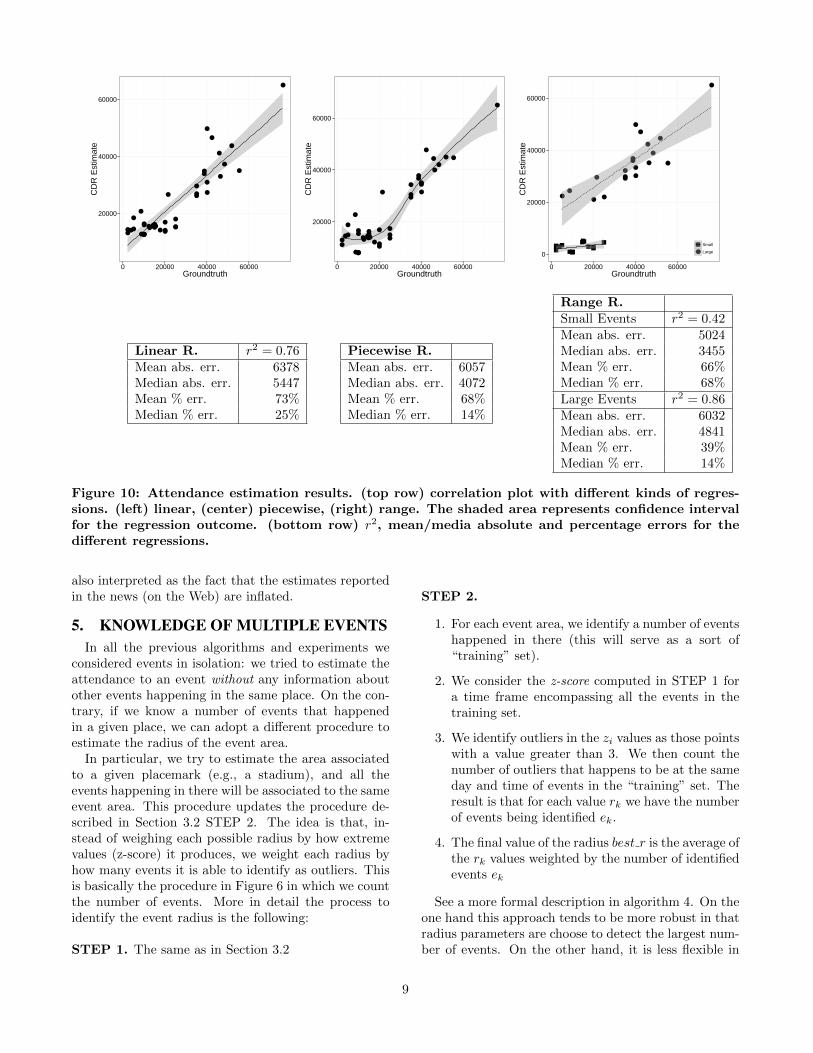
Figure 10(top-row) illustrates the result of the dif-ferent regressions between groundtruth data and ourattendance estimator. Other than visually, we verifiedthat in the case of linear regression (left plot), the re-sults exhibit a Pearson correlation r = 0.87 and a co-efficient of determination r2 = 0.76 indicating a strongpositive correlation between the results. In the caseof piecewise regression (center plot) summarizing a sin-gle correlation coefficient is problematic. However, it ispossible to see a good fit of the data. In the case ofrange linear regression (right plot), r = 0.65/r2 = 0.42for small events (< 10000 persons), r = 0.93/r2 = 0.86for large events (≥ 10000 persons), indicating offeringweak results for small events, while strong correlationfor large ones.

In all the plots, confidence intervals for the regressionis depicted with a gray area.

Figure 10(bottom-row) illustrates mean/median ab-solute error between estimated attendees and groundtruth,and mean/median percentage error (absolute error di-vided by groundtruth). The gap in errors between meanand median indicates that the distribution of error isskewed (in the case of linear regression, skewness =3.10, in the case of piecewise linear regression skew-ness = 2.69, in the case of range regression, skewness =-0.6/3.3 for small and large events respectively). This

is due to the fact that even small errors in the orderof 1000 person would be very high in events with 2000attendees (50% error) thus notably increasing the meanerror.

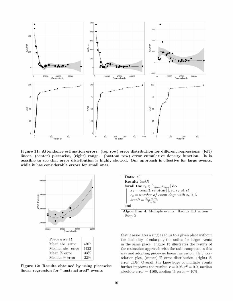
To better quantify this behavior, Figure 11 shows er-ror distribution with regard to groundtruth attendance(top-row) and the error CDF (bottom-row). The graphshows results for linear regression (left), piecewise linearregression (center), range regression (right). Looking atthe graph, it is easy to see the skewness effect describedabove. In all the regressions, rather expectedly, the ap-proach presents large errors for small events, while smallerrors for large events.

In summary, it is possible to see that the use of thedescribed approach produces rather good estimates ofthe number of attendees. It is easy to see that resultsare better in large events where a limited absolute er-ror has a small impact in the overall percent error. Ingeneral, we found that the proposed approach startsproducing consistent good results for events larger than10000 attending persons. Considering only those eventswith an attendance greater than 10000, Pearson corre-lation jumps to 0.93. Linear regression’s mean %errordrops to 22% and median %error drops to 15%. Sim-ilarly, piecewise linear regression’s mean %error dropsto 16% and median %error drops to 13%.

4.3 Unstructured EventsThe dataset of events used for the experiments com-

prises two kinds of events: (i) “structured” events, likeconcerts and football matches, for which some sort ofentrance policy (e.g., entrance gates) allow to obtainreliable estimate on the number of attending persons.(ii) “unstructured” events happening in open squaresor parks for which no entrance policy is enforced. Theanalysis of this latter kind of events is problematic be-cause it is very difficult to obtain reliable groundtruthattendance estimates, however – for the same reason– it is also the best scenario for the actual use of theproposed technique.

Figure 12 illustrate results for a set of “unstructured”events. We fit the linear regression by using “struc-tured” events (football matches in stadiums) happeningin the same city and we searched the Web for reportedattendance estimates and use them as ground truth. Inthis case results are worse than in the previous case,obtaining 22% median %error. On the one hand, thisis due to the fact that these events tends to be smallerthan “structured” ones, thus making the attendance es-timation task inherently more difficult. On the otherhand, the linear regression is trained for larger “struc-tured” events, thus it can be a less effective fit for theseevents. Finally, as groundtruth estimate for this eventsis weaker, the fact that a number of events have an esti-mated attendance lower than the groundtruth might be

8

●

●

●

●

●

●

●

●●

● ●●●

●

●

●

●

●

●●

●

●

●

●

●

●

●

● ●●

●●

●

●

●

● ●

●

●●

●●

●

●

●

●●

●

●

●

●●●●●●●

●

●●

●●●

●

●

●

●

●●

●

●●●

●●

●

●

●● ●

●● ●

●●●

20000

40000

60000

0 20000 40000 60000Groundtruth

CD

R E

stim

ate

●

●

●

●

●

●

●

●●

● ●●●

●

●

●

●●

●●

●

●

●

●

●

●

●

●●

●

●●

●

●

●

●●●

● ●

●●●

●

●

●

●

●

●●

●●

●●●●

●

●

●●●●●

●

●●

●

●

●

●

●●●

●●

●

●

●● ●●● ●

●●●

20000

40000

60000

0 20000 40000 60000Groundtruth

CD

R E

stim

ate

●

●

●●

●

●

●

●

●

●

●

●

● ●●

●

●

● ●●

●

●

●●

●

●

●

●

●

●

●

●

● ●●

●

●● ●●

0

20000

40000

60000

0 20000 40000 60000Groundtruth

CD

R E

stim

ate

●●

Small

Large

Linear R. r2 = 0.76Mean abs. err. 6378Median abs. err. 5447Mean % err. 73%Median % err. 25%

Piecewise R.Mean abs. err. 6057Median abs. err. 4072Mean % err. 68%Median % err. 14%

Range R.Small Events r2 = 0.42Mean abs. err. 5024Median abs. err. 3455Mean % err. 66%Median % err. 68%Large Events r2 = 0.86Mean abs. err. 6032Median abs. err. 4841Mean % err. 39%Median % err. 14%

Figure 10: Attendance estimation results. (top row) correlation plot with different kinds of regres-sions. (left) linear, (center) piecewise, (right) range. The shaded area represents confidence intervalfor the regression outcome. (bottom row) r2, mean/media absolute and percentage errors for thedifferent regressions.

also interpreted as the fact that the estimates reportedin the news (on the Web) are inflated.

5. KNOWLEDGE OF MULTIPLE EVENTSIn all the previous algorithms and experiments we

considered events in isolation: we tried to estimate theattendance to an event without any information aboutother events happening in the same place. On the con-trary, if we know a number of events that happenedin a given place, we can adopt a different procedure toestimate the radius of the event area.

In particular, we try to estimate the area associatedto a given placemark (e.g., a stadium), and all theevents happening in there will be associated to the sameevent area. This procedure updates the procedure de-scribed in Section 3.2 STEP 2. The idea is that, in-stead of weighing each possible radius by how extremevalues (z-score) it produces, we weight each radius byhow many events it is able to identify as outliers. Thisis basically the procedure in Figure 6 in which we countthe number of events. More in detail the process toidentify the event radius is the following:

STEP 1. The same as in Section 3.2

STEP 2.

1. For each event area, we identify a number of eventshappened in there (this will serve as a sort of“training” set).

2. We consider the z-score computed in STEP 1 fora time frame encompassing all the events in thetraining set.

3. We identify outliers in the zi values as those pointswith a value greater than 3. We then count thenumber of outliers that happens to be at the sameday and time of events in the “training” set. Theresult is that for each value rk we have the numberof events being identified ek.

4. The final value of the radius best r is the average ofthe rk values weighted by the number of identifiedevents ek

See a more formal description in algorithm 4. On theone hand this approach tends to be more robust in thatradius parameters are choose to detect the largest num-ber of events. On the other hand, it is less flexible in

9

●●

●●

●●

●

●●

●

●●●●

●

●

●

●

●●

●

●●●

●

●

●●

●● ●● ●

●

●

●

●●

●

●

●

●

●

●●

●●●●

●●●

●●●● ● ●

●

●

●

●●

●●● ●

●

●

●●●● ●● ●

●●

●

●●

●

●●

●

●

0

200

400

0 20000 40000 60000Groundtruth

% E

rror

●●●

● ●●

●

●●

●

●●●

●

●

●

●

●

●●

●

●● ●

●

●

●

●

●●

●● ●

●

●

●

●●

●

●

●

●

●

●● ●● ●●●

●●

●●●●

●●

●

●

●

●●●

●● ●

●

●

●

●●● ●● ●

●●

●

●●

●

●

●

●

●

0

100

200

300

400

500

0 20000 40000 60000Groundtruth

% E

rror

●●

●

●

●●

●

●●● ●●●

●

●●

●

●

●●

●

●●●

●

●● ●

●

●

●

●●

●●

●●

●●

●●●

●●●●●●●

●●

●

●

●●

●●● ●

●

●● ●

●

●

●

●●

●●

−100

0

100

200

300

0 20000 40000 60000Groundtruth

% E

rror

●●●●●●●●●●●●●●●●●●●●●●●●●●●●●●●●●●●●●●●●●●●●●●●●●●●●●●●●●●●●●●●●●●●●●●●●●●●●●●●●

●●●●

●●

●●

●●

●●●

●●

●●

●●●

0

25

50

75

100

0 200 400% Error

CD

F

●●●●●●●●●●●●●●●●●●●●●●●●●●●●●●●●●●●●●●●●●●●●●●●●●●●●●●●●●●●●●●●●

●●●●●●●●●●●●●●●●●●

●●

●●

●●

●●

●●●

●●

●●

●●●

0

25

50

75

100

0 100 200 300 400 500% Error

CD

F

●●●●●●●●●●●●●●●●●●●●●●●●●●●●●●●●●●●●●●●●●●●●●●●●●●●●●●●●●●●●●

●●

●●●●●●●

●●●●●●●●●●●●●●●●●●●●●

●●

●●

●●

●●●

0

25

50

75

100

0 100 200 300% Error

CD

FFigure 11: Attendance estimation errors. (top row) error distribution for different regressions: (left)linear, (center) piecewise, (right) range. (bottom row) error cumulative density function. It ispossible to see that error distribution is highly skewed. Our approach is effective for large events,while it has considerable errors for small ones.

●●

●

●

●

●●

●

●

●

●

●●

●

●

●

● ●

●

●●

●

10000

20000

30000

40000

10000 20000 30000 40000Groundtruth

CD

R E

stim

ate

Piecewise R.Mean abs. error 7307Median abs. error 4422Mean % error 33%Median % error 22%

Figure 12: Results obtained by using piecewiselinear regression for “unstructured” events

Data: z[ ]Result: bestRforall the rk ∈ [rmin, rmax] do

xk = countUsers(cdr[ ], ec, rk, st, et)ek = number of event days with zk > 3

bestR =∑

k rk·ek∑k ek

end

Algorithm 4: Multiple events. Radius Extraction- Step 2

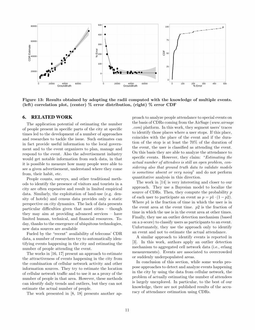
that it associates a single radius to a given place withoutthe flexibility of enlarging the radius for larger eventsin the same place. Figure 13 illustrates the results ofthe estimation approach with the radii computed in thisway and adopting piecewise linear regression. (left) cor-relation plot, (center) % error distribution, (right) %error CDF. Overall, the knowledge of multiple eventsfurther improves the results: r = 0.95, r2 = 0.9, medianabsolute error = 4160, median % error = 10%.

10

●

●

●

●

●●

●

●●

● ●●●

●

●

●

●

●

●

●

●

●

●

●

●●

●● ●●

●●

●

●

●

●●●

●

●

●

●●

●

●

●

●

●●

●

●●

●●●●

●

●

●

●

●

●

●

●

●●

●

●●

●●●●

●●

●

●●

● ●●●

●●

●●

20000

40000

60000

80000

0 20000 40000 60000Groundtruth

CD

R E

stim

ate

●●●● ●

●●

●●

●

●●●

●●

●

●

●

●

●

●

●● ●

●

●

●

●

●

●

●● ●●●

●

●●

●

●●

●

●

●● ●● ●●●

●●●●●●

● ●

●

●

●

●

●●

●● ●

●

●

●

●●

●

●● ●●●

●

●●

●

● ●

●

●

0

100

200

300

400

500

0 20000 40000 60000Groundtruth

% E

rror

●●●●●●●●●●●●●●●●●●●●●●●●●●●●●●●●●●●●●●●●●●●●●●●●●●●●●●●

●●●●●●●●●●●●●●●●●●●●●●●●●●●●●●●

●●

●●

●●

●●

●●

●●●●

0

25

50

75

100

0 100 200 300 400 500% Error

CD

F

Figure 13: Results obtained by adopting the radii computed with the knowledge of multiple events.(left) correlation plot, (center) % error distribution, (right) % error CDF

6. RELATED WORKThe application potential of estimating the number

of people present in specific parts of the city at specifictimes led to the development of a number of approachesand researches to tackle the issue. Such estimates canin fact provide useful information to the local govern-ment and to the event organizers to plan, manage andrespond to the event. Also the advertisement industrywould get notable information from such data, in thatit is possible to measure how many people were able tosee a given advertisement, understand where they comefrom, their habit, etc.

People counts, surveys, and other traditional meth-ods to identify the presence of visitors and tourists in acity are often expensive and result in limited empiricaldata. Similarly, the exploitation of land-use (e.g. den-sity of hotels) and census data provides only a staticperspective on city dynamics. The lack of data presentsparticular difficulties given that most cities – thoughthey may aim at providing advanced services – havelimited human, technical, and financial resources. To-day, thanks to the emergence of ubiquitous technologies,new data sources are available

Fueled by the “recent” availability of telecoms’ CDRdata, a number of researchers try to automatically iden-tifying events happening in the city and estimating thenumber of people attending the event.

The works in [16, 17] present an approach to estimatethe attractiveness of events happening in the city fromthe combination of cellular network activity and otherinformation sources. They try to estimate the locationof cellular network traffic and to use it as a proxy of thenumber of people in that area. However, these methodscan identify daily trends and outliers, but they can notestimate the actual number of people.

The work presented in [8, 18] presents another ap-

proach to analyze people attendance to special events onthe basis of CDRs coming from the AirSage (www.airsage.com) platform. In this work, they segment users’ tracesto identify those places where a user stops. If this place,coincides with the place of the event and if the dura-tion of the stop is at least the 70% of the duration ofthe event, the user is classified as attending the event.On this basis they are able to analyze the attendance tospecific events. However, they claim: “Estimating theactual number of attendees is still an open problem, con-sidering also that ground truth data to validate modelsis sometime absent or very noisy” and do not performquantitative analysis in this direction.

The work in [14] is very interesting and closer to ourapproach. They use a Bayesian model to localize thesource of CDRs. Then, they compute the probability pof each user to participate an event as p = p1 · (1− p2).Where p1 is the fraction of time in which the user is inthe event area at the event time. p2 is the fraction oftime in which the use is in the event area at other times.Finally, they use an outlier detection mechanism (basedon a z-score) to classify users as participants to an event.Unfortunately, they use the approach only to identifyan event and not to estimate the actual attendance.

A similar approach to identify events is reported in[3]. In this work, authors apply an outlier detectionmechanism to aggregated cell network data (i.e., erlangmeasurements). Events are associated to overcrowdedor suddenly underpopulated areas.

In conclusion of this section, while some works pro-pose approaches to detect and analyze events happeningin the city by using the data from cellular network, theproblem of actually estimating the number of attendeesis largely unexplored. In particular, to the best of ourknowledge, there are not published results of the accu-racy of attendance estimation using CDRs.

11

7. CONCLUDING REMARKSIn this work we propose an innovative methodology to

estimate the number of attendees to events happeningin the city from cellular network data. We evaluate ourapproach in 43 events ranging from football matchesin stadiums to concerts and festivals in open squares.Comparing our results with the best groundtruth dataavailable, our estimates provide a median error of lessthan 15% of the actual number of attendees.

While the obtained results are very encouraging, thereare a number of research directions that could improvethe presented work:

• Of course, running experiments on other, more di-verse, events would better validate our results.

• Our work has been mainly driven by experiments.A better theoretical framework for our modeling(especially with regard to the event area estima-tion) could provide further ideas for improvement.

• A deeper analysis of the trajectories of individualusers could provide a more fine grained localizationof CDRs, thus leading to a better estimate of theuser’s presence in the event area [6]

Despite the above limitations, to the best of our knowl-edge, this is the first work providing a practical andaccurate way of estimating the number of attendees toevents happening in the city from cellular network data.

8. REFERENCES[1] F. Calabrese, C. Ratti, M. Colonna, P. Lovisolo,

D. Parata, Real-time urban monitoring using cellphones: a case study in rome, IEEE Transactionson Intelligent Transportation Systems 12 (1)(2011) 141–151.

[2] L. Ferrari, M. Mamei, Discovering city dynamicsthrough sports tracking applications, IEEEComputer 44 (12) (2011) 61–66.

[3] L. Ferrari, M. Mamei, M. Colonna, Discoveringevents in the city via mobile network analysis,Journal of Ambient Intelligence and HumanizedComputing 5 (3) (2014) 265–277.

[4] R. Becker, R. Caceres, K. Hanson, S. Isaacman,J. M. Loh, M. Martonosi, J. Rowland, S. Urbanek,A. Varshavsky, C. Volinsky, Human mobilitycharacterization from cellular network data,Communications of the ACM 56 (1) (2013) 74–82.

[5] F. Zambonelli, Toward sociotechnical urbansuperorganisms, IEEE Computer 45 (8) (2012)76–78.

[6] I. Leontiadis, A. Lima, H. Kwak, R. Stanojevic,D. Wetherall, K. Papagiannaki, From cells tostreets: Estimating mobile paths withcellular-side data, in: International Conference on

emerging Networking EXperiments andTechnologies (CoNEXT), Sydney, Australia, 2014.

[7] N. Lathia, V. Pejovic, K. Rachuri, C. Mascolo,M. Musolesi, P. Rentfrow, Smartphones forlarge-scale behaviour change intervention, IEEEPervasive Computing 12 (2013) 66–73.

[8] D. Quercia, G. D. Lorenzo, F. Calabrese,C. Ratti, Mobile phones and outdoor advertising:Measurable advertising, IEEE PervasiveComputing 10 (2) (2011) 28–36.

[9] D. J. Mir, S. Isaacman, R. Caceres, M. Martonosi,R. N. Wright, Dp-where: Differentially privatemodeling of human mobility, in: IEEEInternational Conference on Big Data, SantaClara (CA), USA, 2013.

[10] A. Basu, A. Monreale, J. C. Corena, F. Giannotti,D. Pedreschi, S. Kiyomoto, Y. Miyake,T. Yanagihara, R. Trasarti, A privacy risk modelfor trajectory data, in: International IFIPConference on Trust Management, Singapore,2014.

[11] M. Rahnema, Overview of the gsm system andprotocol architecture, IEEE Communications31 (4) (1993) 92–100.

[12] R. Caceres, J. Rowland, C. Small, S. Urbanek,Exploring the use of urban greenspace throughcellular network activity, in: Workshop onPervasive Urban Applications (PURBA),Newcastle, UK, 2012.

[13] M. Ulm, P. Widhalm, Properties of thepositioning error of cell phone trajectories, in:NetMob, Boston (MA), USA, 2013.

[14] V. A. Traag, A. Browet, F. Calabrese, F. Morlot,Social event detection in massive mobile phonedata using probabilistic location inference, in:International Conference on Social Computing,Boston (MA), USA, 2011.

[15] M. Gonzalez, C. Hidalgo, A. Barabasi,Understanding individual human mobilitypatterns, Nature 453 (2008) 779–782.

[16] F. Girardin, A. Vaccari, A. Gerber, A. Biderman,C. Ratti, Quantifying urban attractiveness fromthe distribution and density of digital footprints,International Journal of Spatial DataInfrastructure Research 4 (2009) 175–200.

[17] J. Neumann, M. Zao, A. Karatzoglou, N. Oliver,Event detection in communication andtransportation data, Pattern Recognition andImage Analysis 7887 (2013) 827–838.

[18] F. Calabrese, F. Pereira, G. Lorenzo, L. Liang,C. Ratti, The geography of taste: Analyzingcell-phone mobility and social events, in:International Conference on PervasiveComputing, Helsinki, Finland, 2010.

12