Embed Size (px)
Citation preview
Estimating Data Integration and Cleaning Effort
Sebastian KruseHasso Plattner Institute (HPI),
Paolo PapottiQatar Computing Research
Institute (QCRI), [email protected]
Felix NaumannHasso Plattner Institute (HPI),
ABSTRACTData cleaning and data integration have been the topic of intensiveresearch for at least the past thirty years, resulting in a multitude ofspecialized methods and integrated tool suites. All of them requireat least some and in most cases significant human input in theirconfiguration, during processing, and for evaluation. For managers(and for developers and scientists) it would be therefore of greatvalue to be able to estimate the effort of cleaning and integratingsome given data sets and to know the pitfalls of such an integrationproject in advance. This helps deciding about an integration projectusing cost/benefit analysis, budgeting a team with funds and man-power, and monitoring its progress. Further, knowledge of howwell a data source fits into a given data ecosystem improves sourceselection.
We present an extensible framework for the automatic effort es-timation for mapping and cleaning activities in data integrationprojects with multiple sources. It comprises a set of measures andmethods for estimating integration complexity and ultimately ef-fort, taking into account heterogeneities of both schemas and in-stances and regarding both integration and cleaning operations. Ex-periments on two real-world scenarios show that our proposal istwo to four times more accurate than a current approach in esti-mating the time duration of an integration process, and provides ameaningful breakdown of the integration problems as well as therequired integration activities.
1. COMPLEXITY OF INTEGRATION ANDCLEANING
Data integration and data cleaning remain among the mosthuman-work-intensive tasks in data management. Both require aclear understanding of the semantics of schema and data – a no-toriously difficult task for machines. Despite much research anddevelopment of supporting tools and algorithms, state-of-the-art in-tegration projects involve significant human resource cost. In fact,Gartner reports that 10% of all IT cost goes into enterprise software
c�2015, Copyright is with the authors. Published in Proc. 18th Inter-national Conference on Extending Database Technology (EDBT), March23-27, 2015, Brussels, Belgium: ISBN 978-3-89318-067-7, on OpenPro-ceedings.org. Distribution of this paper is permitted under the terms of theCreative Commons license CC-by-nc-nd 4.0.
for data integration and data quality1,2, and it is well recognized thatmost of those expenses are for human labor. Thus, when embarkingon a data integration and cleaning project, it is useful and impor-tant to estimate in advance the effort and cost of the project and tofind out which particular difficulties cause these. Such estimationshelp deciding whether to pursue the project in the first place, plan-ning and scheduling the project using estimates about the durationof integration steps, budgeting in terms of cost or manpower, andfinally monitoring the progress of the project. Cost estimates canalso help integration service providers, IT consultants, and IT toolvendors to generate better price quotes for integration customers.Further, automatically generated knowledge of how well and howeasy a data source fits into a given data ecosystem improves sourceselection.
However, “project estimation for [. . . ] data integration projectsis especially difficult, given the number of stakeholders involvedacross the organization as well as the unknowns of data complexityand quality.” [14]. Any integration project has several steps andtasks, including requirements analysis, selection of data sources,determining the appropriate target database, data transformationspecifications, testing, deployment, and maintenance. In this pa-per, we focus on exploring the database-related steps of integrationand cleaning and automatically estimate their effort.
1.1 ChallengesThere are simple approaches to estimate in isolation the com-
plexity of individual mapping and cleaning tasks. For the mapping,evaluating its complexity can be done by counting the matchings,i.e., correspondences, among elements. For the cleaning problem, anatural solution is to measure its complexity by counting the num-ber of constraints on the target schema. However, as several inte-gration approaches have shown, the interactive nature of these twoproblems is particularly complex [5, 11, 13]. For example, a dataexchange problem takes as input two relational schemas, a trans-formation between them (a mapping), a set of target constraints,and answers two questions: whether it is possible to compute avalid solution for a given setting and how. Interestingly, to have asolution, certain conditions must hold on the target constraints, andextending the setting to more complex languages or data modelsbring tighter restrictions on the class of tractable cases [6, 12].
In our work, the main challenge is to estimate complexity andeffort in a setting that goes beyond these ad-hoc studies while sat-isfying four main requirements:
Generality: We require independence from the language used toexpress the data transformation. Furthermore, real cases often failthe existence of solution tests considered in formal frameworks,
1http://www.gartner.com/ technology/research/ it-spending-forecast/2http://www.gartner.com/newsroom/ id/2292815
61 10.5441/002/edbt.2015.07

e.g., weak acyclicity condition [11], but an automatic estimation isstill desirable for them in practice.
Completeness: Only a subset of the constraints that hold on thedata are specified over the schema. In fact, business rules are com-monly enforced at the application level and are not reflected in themetadata of the schemas, but should nevertheless be considered.
Granularity: Details about the integration issues are crucial forconsumption of the estimation. For a real understanding and properplanning, it is important to know which source and/or target at-tributes are cause of problems and how, e.g., phone attributes insource and target schema have different formats. Existing estima-tors do not reason over actual data structures and thus make nostatements about the causes of integration effort.
Configurability and extensibility: The actual effort depends onsubjective factors, such as the capabilities of available tools andthe desired quality of the output. Therefore, intuitive, yet rich con-figuration settings for the estimation process are crucial for its ap-plicability. Moreover, users must be able to extend the range ofproblems covered by the framework.
These challenges cannot be tackled with existing syntacticalmethods to test the existence of solutions, as they work only inspecific settings (Generality), are restricted to declarative specifica-tions over the schemas (Completeness), and do not provide detailsabout the actual problems (Granularity). On the other hand, as sys-tems that compute solutions require human interaction to finalizethe process [8, 13], they cannot be used for estimation purpose andtheir availability is orthogonal to our problem (Configurability).
1.2 Approaching Effort EstimationFigure 1 presents our view on the problem of estimating the ef-
fort of data integration. The starting point is an integration sce-nario with a target database and one or more source databases. Theright-hand side of the figure shows the actual integration processperformed by an integration specialist, where the goal is to moveall instances of the source databases into the target database. Typ-ically, a set of integration tools are used by the specialist. Thesetools have access to the source and target and support her in thetasks. The process takes a certain effort, which can be measured,for instance as amount of work in hours or days or in a monetaryunit.
Our goal is to find that effort without actually performing the in-tegration. Moreover, we want to find and present the problems thatcause this effort. To this end, we developed a two-phase process asshown on the left-hand side of Figure 1.
The first phase, the complexity assessment, reveals concreteintegration challenges for the scenario. To address generality,these problems are exclusively determined by the source and tar-get schemas and instances; if and how an integration practitionerdeals with them is not addressed at this point. Thus, this first phaseis independent of external parameters, such as the level of expertiseof the specialist or the available integration tools. However, it isaided by the results of schema matching and data profiling tools,which analyze the participating databases and produce metadataabout them (to achieve completeness). The output of the complex-ity assessment is a set of clearly defined problems, such as numberof violations for a constraint or number of different value represen-tations. This detailed breakdown of the problems achieves granu-larity and is useful for several tasks, even if not interpreted as aninput to calculate actual effort. Examples of application are sourceselection [9], i.e., given a set of integration candidates, find thesource with the best ‘fit’; and support for data visualization [7],i.e., highlight parts of the schemas that are hard to integrate.
Data Integration
Scenario
Complexity Assessment
Integration Practitioner
Estimated Complexity
Integration Result
Measured Effort
Estimated Effort
Estimation Side Production Side
Integration Tools
influence
estimates
Effort Estimation
Schema Matching
Data Profiling
Figure 1: Overview of effort estimation and execution of data inte-gration scenarios.
The second phase, effort estimation, builds upon the complexityassessment to estimate the actual effort for overcoming the previ-ously revealed integration challenges in some useful unit, such asworkdays or monetary cost. Thereby, this phase addresses config-urability by taking external parameters into account, such as theexperience of the integration practitioner and the features of theintegration tools to be used.
1.3 Contributions and structureSection 2 presents related work and shows that we are the first to
systematically address a dimension of data integration and cleaningthat has been passed over by the database community but is relevantto practitioners. In particular, we make the following contributions:
• Section 3 introduces the extensible Effort Estimation frame-work (EFES), which defines a two-dimensional modulariza-tion of the estimation problem.
• Section 4 describes an estimation module for structural con-flicts between source and target data. This module incorpo-rates a new formalism to compare schemas in terms of map-pings and constraints.
• Section 5 reports an estimation module for value hetero-geneities that captures formatting problems and anomaliesin data that may be missed by structural conflicts.
These building blocks have been evaluated together in an exper-imental study on two real-world datasets and Section 6 reports onthe results. Finally, we conclude our insights in Section 7.
2. RELATED WORKWhen surveying computer science literature, a pattern becomes
apparent: much technology claims (and experimentally shows) toreduce human effort. The veracity of this claim is evident – af-ter all, any kind of automation of tedious tasks is usually helpful.While for scientific papers this reduction is enough of a claim, theabsolute measures of effort and its reduction are rarely explainedand measured.
General effort estimation. There are several approaches for ef-fort estimation in different fields, however, none of them considersinformation coming from the datasets.
62
In the software domain, an established model to estimate the costof developing applications is COCOMO [3, 4], which is based onparameters provided by the users such as the number of lines ofexisting code. Another approach decomposes an overall work taskinto a smaller set of tasks in a “work breakdown structure” [16].The authors manually label business requirements with an effortclass of simple, medium, or complex, and multiply each of themby the number of times the task must be executed.
In the ETL context, Harden [14] breaks down a project into var-ious subtasks, including requirements, design, testing, data stew-ardship, production deployment, but also the actual developmentof the data transformations. For the latter he uses the number ofsource attributes and assigns for each attribute a weighted set oftasks (Table 1). In sum, he calculates slightly more than 8 hours ofwork for each source attribute.
Task Hours per attributeRequirements and Mapping 2.0High Level Design 0.1Technical Design 0.5Data Modeling 1.0Development and Unit Testing 1.0System Test 0.5User Acceptance Testing 0.25Production Support 0.2Tech Lead Support 0.5Project Management Support 0.5Product Owner Support 0.5Subject Matter Expert 0.5Data Steward Support 0.5
Table 1: Tasks and effort per attribute from [14].
One can find other lists of criteria to be taken into account whenestimating the effort of an integration project3. These include fac-tors we include in our complexity model, such as number of dif-ferent sources and types, duplicates, schema constraints, and oth-ers we exclude for sake of space from our discussion, such asproject management, deployment needs, and auditing. There arealso mentions of factors that influence our effort model, such asfamiliarity with the source database, skill levels, and tool avail-ability. However, merely providing a list of factors is only a firststep, whereas we provide novel measures for the database-specificcauses for complexity and effort. In fact, existing methods: (i) lacka direct numerical analysis of the schemas and datasets involved inthe transformation and cleaning; (ii) do not regard the properties ofthe datasets at a fine grain and cannot capture the nature of the pos-sible problems in the scenario, (iii) do not consider the interactionof the mapping and the cleaning problems.
Schema-matching for effort estimation. In our work, we ex-ploit schema matching to bootstrap the process. This is alongthe lines of what authors of matchers suggested. For example,in [24] the authors have pointed out the multiple usages of schemamatching tools beyond the concrete generation of correspondencesfor schema mappings. In particular, they mention “project plan-ning” and “determining the level of effort (and corresponding cost)needed for an integration project”. In a similar fashion, in the eval-uation of the similarity flooding algorithm, Melnik et al. proposea novel measure “to estimate how much effort it costs the user to
3Such as http://www.datamigrationpro.com/data-migration-articles/2012/2/9/data-migration-effort-estimation-practical-techniques-from-r.html and http://www.information-management.com/news/1093630-1.html
modify the proposed match result into the intended result” in termsof additions and deletions of matching attribute pairs [19].
Data-oriented effort estimation. In [25], the authors offer a“back of the envelope” calculation on the number of comparisonsneeded to be performed by human workers to detect duplicates ina dataset. According to them, the estimate depends on the way thepotential duplicates are presented, in particular their order and theirgrouping. Their ideas fit well into our effort model and show thatspecific tooling indeed changes the needed effort, independentlyof the complexity of the problem itself. Complementary work onsource selection has focused on the benefit of integrating a newsource based on its marginal gain [9, 23].
Data-cleaning and data-transformation. Many systems(e.g., [8, 13]) address the problem of detecting violations over thedata given a set of constraints, as we also do in one of our mod-ules for complexity estimation. The challenge for these systemsis mostly the automatic repair step, i.e., how to update the data tomake it consistent wrt. the given constraints with a minimal num-ber of changes. None of these systems provide tools to estimate thecomplexity of the repair nor the user effort before actually execut-ing the methods to solve the integration problem. In fact, the chal-lenge is that solving the problem involves the users, and estimatingthis effort (even in presence of these tools) is our main goal. Similarproblems apply to data exchange and data transformation [1, 15].
In the field of model management, the use of metamodels hasbeen investigated to represent in a more general language severalalternative data models [2,21]. Our cardinality-constrained schemagraphs (Section 4) can be seen as a proposal for a metamodel witha novel static analysis of cardinalities to identify problems in theunderlying schemas and the mapping between them.
3. THE EFFORT ESTIMATION FRAME-WORK
Real-world data integration scenarios host a large number of dif-ferent challenges that must be overcome. Problems arise in com-mon activities, such as the definition of a mapping between differ-ent schemas, the restructuring of the data, and the reconciliationof their value format. We first describe these problems and thenintroduce our solution.
3.1 Data Integration ScenarioA data integration scenario comprises: (i) a set of source
databases; (ii) a target database, into which the source databasesshall be integrated; and (iii) correspondences to describe how thesesources relate to the target. Each source database consists of a rela-tional schema, an instance of this schema, and a set of constraints,which must be satisfied by that instance. Likewise, the target data-base can carry constraints and possibly already contains data aswell that satisfies these constraints. Furthermore, each correspon-dence connects a source schema element with the target schemaelement, into which its contents should be integrated.
Oftentimes constraints are not enforced at the schema level butrather at the application level or simply in the mind of the inte-gration expert. Even worse, for some sources (e.g., data dumps),a schema definition may be completely missing. To achieve com-pleteness, techniques for schema reverse engineering and data pro-filing [20] can reconstruct missing schema descriptions and con-straints from the data.
Example 3.1. Figure 2 shows an integration scenario with mu-sic records data. Both source and target relational schemas (Fig-ure 2a) define a set of constraints, such as primary keys (e.g., id in
63

Target
tracks
recordtitleduration
FK,NNNN
records
idtitleartistgenre
PKNNNN
albums
idnameartist_list
PKNNFK,NN
songs
albumnameartist_listlength
FKNNFK
artist_lists
idPK
artist_credits
artist_listpositionartist
PK,FKPKNN
Source
(a) Schemas, constraints, and correspondences.
record title duration1 “Sweet Home Alabama" “4:43"1 “I Need You" “6:55"1 “Don’t Ask Me No Questions" “3:26"
...
(b) Example instances from the target table tracks.
album name artist_list lengths3 “Hands Up" a1 215900s3 “Labor Day" a1 238100s3 “Anxiety" a2 218200
...
(c) Example instances from the source table songs.
Figure 2: An example data integration scenario.
records), foreign keys (record in tracks, represented with dashedarrows), and not nullable values (title in tracks).
Solid arrows between attributes and relations represent corre-spondences, i.e., two attributes that store the same atomic infor-mation or two relations that store the same kind of instances. Thesource relation albums corresponds to the target relation records
and its source attribute name corresponds to the title attribute inthe target. That means, that the albums from the source shall beintegrated as records into the target, while the source album namesserve as titles for the integrated records. ⇧
We assume correspondences between the source and targetschemas to be given, as they can be automatically discovered withschema matching tools [10]. Notice that correspondences are notan executable representation of a transformation, thus they do notinduce a precise mapping between sources and the target. However,they contain enough information to reason over the complexity ofdata integration scenarios and detect their integration challenges, asin the following example.
Example 3.2. The target schema requires exactly one artistvalue per record, whereas the source schema can associate an arbi-trary number of artist credits to each album. This situation impliesthat integrating any source album with zero artist credits violatesthe not-null constraint on the target attribute records.artist. More-over, two or more artist credits for a single source album cannotbe naturally stored by the single target attribute. Integration prac-titioners have to solve these conflicts. Hence, this schema hetero-geneity increases the necessary effort to achieve the integration. ⇧
Not all kinds of integration issues can be detected by analyzingthe schemas, though. The data itself is equally important. Whilewe assume that every instance is valid wrt. its schema, when data isintegrated new problems can arise. For example, all sources mightbe free of duplicates, but there still might be target duplicates whenthey are combined [22]. These conflicts can also arise betweensource data and pre-existing target data.
Example 3.3. Tables 2b and 2c report sample instances of thetracks table and the songs table, respectively. The duration oftracks in the target database is encoded as a string with the for-mat m:ss, while the length of songs is measured in milliseconds inthe source. The two formats are locally consistent, but the sourcevalues need a proper transformation when integrated into the targetcolumn, thereby demanding a certain amount of effort. ⇧
3.2 A General FrameworkFacing different kinds of data integration and cleaning actions,
there is the need of different specialized models to decode theircomplexity and estimate their effort properly. We tackle this prob-lem with our general effort estimation framework EFES. It handlesdifferent kinds of integration challenges by accepting a dedicatedestimation module to cope with each of them independently. Suchmodularity makes it easier to revise and refine individual modulesand establishes the desired extensibility by plugging new ones. Inthis work, we present modules for the three general and, in our ex-perience, most common classes of integration activities: writing anexecutable mapping, resolving structural conflicts, and eliminatingvalue heterogeneities. While the latter two are explained in subse-quent sections, we present the mapping module in this section toexplain our framework design. For generality, the modules do notdepend on a fixed language to express the transformations.
Figure 3 depicts the general architecture of EFES. The architec-ture implements our goal of delivering a set of integration problemsand an effort estimate by explicitly dividing the estimation processinto an objective complexity assessment, which is based on proper-ties of schemas and data, followed by the context-dependent effortestimation. We now describe these two phases in more detail.
Data Integration Scenario
Effort Estimate
Data Complexity Reports
Data Complexity
Detectors
TaskPlanners
Effort Calculation
Functions
Com
plex
ity A
ssem
ent
Effo
rt E
stim
atio
n
Estimation Module
Expected Quality
Execution Settings
Tasks
Figure 3: Architecture of EFES.
3.3 Complexity assessmentThe goal of this first phase is to compute data complexity reports
for the integration scenario. These reports serve as the basis for the
64

subsequent effort estimation but also are used to inform the userabout integration problems within the scenario. This is particularlyuseful for source selection [9] and data visualization [7].
Each estimation module provides a data complexity detector thatextracts complexity indicators from the given scenario and writesthem into its report. There is no formal definition for such a report;rather, it can be tailored to the specific, needed complexity indi-cators. For example, the mapping module builds on the followingidea: For each table in the target schema and each source databasethat provides data for that table, some connection has to be estab-lished to fetch the source data and write it into the target table. Theoverall complexity of the mapping creation is composed of the in-dividual complexities for establishing each of these connections.Furthermore, every connection can be described in terms of cer-tain metrics, such as the number of source tables to be queried, thenumber of attributes that must be copied, and whether new IDs fora primary key need to be generated.
Example 3.4. The data complexity report for the scenario inFigure 2 can be found in Table 2. To fetch the data for therecords table, the three source tables albums, artist_lists, andartist_credits have to be combined, two attributes must be copied,and unique id values for the integrated tuples must be generated. ⇧
Target table Source tables Attributes Primary keyrecords 3 2 yestracks 3 2 no
Table 2: Mapping complexity report of the scenario in Figure 2.
3.4 Effort estimationBased on the data complexity, the effort estimation shall produce
a single estimate of the human work to address the different com-plexities. However, going from an objective complexity measure toa subjective estimate of human work requires external informationabout the context. We distinguish one aspect that is specific to thedata integration problem, (i) the expected quality of the integrationresult, and, as a more common aspect, (ii) the execution settings forthe scenario.
(i) Expected quality: Data cleaning is the operation of updat-ing an instance such that it becomes consistent wrt. any constraintdefined on its schema [8, 13]. However, such results can be ob-tained by automatically removing problematic tuples, or by man-ually solving inconsistencies involving a domain expert. Eachchoice implies different effort.
Example 3.5. Consider again Example 3.3 with the durationformat mismatch. As duration is nullable, one simple way to solvethe problem is to drop the values coming from the new source. Abetter, higher quality solution is to transform the values to a com-mon format, but this operation requires a script and a validation bythe user, i.e., more effort [15]. ⇧
(ii) Execution settings: The execution settings represent the cir-cumstances under which the data integration shall be conducted.Examples of common context information are the expertise of theintegration practitioners and their familarity with the data [4]. Inour setting, we also model the level of automation of the availableintegration tools, and how critical the errors are, e.g., integratingmedical prescriptions requires more attention (and therefore effort)than integrating music tracks.
Example 3.6. Consider again the problem with the cardinalityof record artists. There are schema mappings tools [18] that areable to automatically create a synthetic value in the target, if asource album has zero artist credits, and to automatically createmultiple occurrences of the same album with different artists, ifmultiple artists are credited for a single source album. Such toolswould reduce the mapping effort. ⇧
For the effort estimation, each estimation module has to providea task planner that consumes its data complexity report and outputstasks to overcome the reported issues. Each of these tasks is of acertain type, is expected to deliver a certain result quality, and com-prises an arbitrary set of parameters, such as on how many tuples ithas to be executed. We defined two instances of expected quality,namely low effort (removal of tuples) and high quality (updates).This criterion is extensible to other repair actions, but it alreadyallows to choose between alternative cleaning tasks as shown inExample 3.5.
Example 3.7. A complexity report for the scenario from Fig-ure 2 states that there are albums without any artist in the sourcedata that lead to a violation of a not-null constraint in the target.The corresponding task model proposes the alternative actions Re-ject violating tuple (low effort) or Add missing value (high quality)to solve the problem. ⇧
Once the list of tasks has been determined, the effort for theirexecution is computed. For this purpose, the user specifies in ad-vance for each task type an effort-calculation function that can in-corporate task parameters. As an example, we report the effort-calculation functions for the execution settings of our experimentsin Table 9. The framework uses these functions to estimate the ef-fort for each of the tasks. Finally, the total of all these task estimatesforms the overall effort estimate.
Example 3.8. We exemplify the effort-calculation functions forthe tasks derived from the report in Table 2. The Create mappingtask might be done manually with SQL queries. Then an adequatefunction would be
effort = 3mins · tables + 1min · attributes + 3mins · PKs
leading to an overall effort of 25 (18 + 4 + 3) minutes. How-ever, if a tool can generate this mapping automatically based onthe correspondences (e.g., [18]), then a constant value, such aseffort = 2mins , can reflect this circumstance, leading to an over-all effort of four minutes. ⇧
The above described task-based approach offers several advan-tages over an immediate complexity-effort mapping [14], where aformula directly converts statistics over the schemas into an effortestimation value. Our model enables configurability, as it treats ex-ecution settings as a first-class component in the effort-calculationfunctions and these can be arbitrarily complex as needed. Further-more, instead of just delivering a final effort value, our effort esti-mate is broken down according to its underlying tasks. This gran-ularity helps users understand the required work and explains howthe estimate has been created, thus giving the users the opportunityto properly plan the integration process.
4. STRUCTURAL CONFLICTSStructural heterogeneities between source and target data struc-
tures are a common problem in integration scenarios. This sectiondescribes a module to detect these problems and estimate the effort
65

arising out of them. It can be plugged into the framework archi-tecture in Figure 3 with the following workflow: Its data complex-ity detector (structure conflict detector) analyzes how source andtarget data relate to each other, and counts the number of emerg-ing structural conflicts. Based on those conflicts, the task planner(structure repair planner) then (i) derives a set of cleaning tasksto make the conflicting source data fit into the target schema, and(ii) estimates how often each such task has to be performed. Thesetasks can finally be fed into the effort calculation functions.
4.1 Structure Conflict DetectorIn the first step of structural conflict handling, all source and
target schemas of the given scenario are converted into cardinality-constrained schema graphs (short CSG), a novel modeling formal-ism that we specifically devised for our task. It offers a single,yet expressive constraint formalism with a set of inference oper-ators that allow elegant comparisons of schemas. Additionally, itis more general than the relational model and can describe (in-tegrated) database instances that do not conform to the relationalmodel. For instance, an integrated tuple might provide multiplevalues for a single attribute, like in Example 3.2. The higher ex-pressiveness of CSGs allows to reason about necessary cleaningtasks to make the integrated databases conform to the relationalmodel. In the following, we formally define CSGs and explain howto convert relational databases into CSGs.
DEFINITION 1. A CSG is a tuple � = (N,P,), where N is aset of nodes and P ⇢ N2 is a set of relationships. Furthermore, : P ! 2
N expresses schema constraints by prescribing cardinal-ities for relationships.
DEFINITION 2. A CSG instance is a tuple I(�) = (IN , IP ),where IN assigns a set of elements to each node in N and IP
assigns to each relationship links between those elements.
To convert a relational schema, for each of its relations, a cor-responding table node (rectangle) is created to represent the exis-tence of tuples in that relation. Furthermore, for each attribute, anattribute node (round shape) is created and connected to its respec-tive table node via a relationship. While these attribute nodes holdthe set of distinct values of the original relational attribute, the re-lationships link tuples and their respective attribute values. Withthis proceeding, any relational database can be turned into a CSGwithout loss of information.
Example 4.1. Figure 4 depicts two CSGs for the example sce-nario schemas in Figure 2a, one for the source and one for thetarget schema4. For instance, the example tracks tuple t = (1,“Sweet Home Alabama”, “4:43”) from Figure 2b is represented inthe CSG instance as follows: The table node tracks 2 N holds anabstract element idt, i.e., idt 2 IN (tracks), representing the tu-ple’s identity. Likewise, record 2 N holds exactly once the value 1,i.e., 1 2 IN (record), and the relationship ⇢
tracks!record
containsa link for these elements, i.e., (idt, 1) 2 IP (⇢tracks!record
), thusstating that t[record] = 1. The other values for the title andduration attributes are represented accordingly. Furthermore, for-eign key relationships are represented by special equality relation-ships (dashed line) that link all equal elements of two nodes, e.g.,all common values of the id and record nodes in the target CSG ofFigure 4. ⇧
4Some correspondences between the schemas are omitted forclarity, but are not generally discarded.
Source
records
artist title genre id1 1
1..*tracks
record title' duration
albums
idnameartist_list
songs
album name' artist_list' length
artist_lists
id'
artist_credits
artist position artist_list''
Target
1..*
0..1
1..*
1
1
0..11
1 1
1..* 1..* 1..*
0..1
1
1
1
1..*
1
1..*
0..11
1
1..*
1
1..*
1
1..*
0..1
1..*
1
0..1
1
10..1
0..1
1..*
1
1..*
1
1..*
1
1
1
Figure 4: The integration scenario translated into cardinality-constrained schema graphs.
To express schema constraints in CSGs, all relationships are an-notated with prescribed cardinalities, that restrict the number ofelements and/or values of connected nodes that must relate to eachother via the annotated relationship. For example, tracks.recordis not nullable, which means, that each tracks tuple must provideexactly one record value. Translated to CSGs, this means that foreach tuple ti, the relationship ⇢
tracks!record
must contain exactlyone link:
8ti : |{v 2 IN (record) | (idti , v) 2 IP (⇢tracks!record
)}| = 1 .
Formally, this is expressed by (⇢tracks!record
) = {1}, which isalso graphically annotated in Figure 4. However, tracks.recordis not subject to a unique-constraint. In consequence, everyrecord value can be found in one or more tuples. Therefore,(⇢
record!tracks
) = 1..⇤ = {1, 2, 3, . . .}. By means of prescribedcardinalities, unique, not-null, and foreign key constraints can beexpressed, as well as two conformity rules for relational schemas:each tuple can have at most one value per attribute, and each at-tribute value must be contained in a tuple.
As stated above, another important feature of CSGs is the abilityto combine relationships into complex relationships and to analyzetheir properties. As one effect, prescribing cardinalities not only toatomic but also to complex relationships further allows to expressn-ary versions of the above constraints and functional dependen-cies. We devised the following relationship construction operators:
‘�’: The composition concatenates two adjacent relationships.Formally, IP (⇢1 � ⇢2)
def= IP (⇢1) � IP (⇢2).
‘[’: The union of two relationships ⇢1[⇢2 contains all links of thetwo relationships, i.e., IP (⇢1 [ ⇢2)
def= IP (⇢1) [ IP (⇢2).
This is particularly useful, when multiple source relation-ships need to be combined.
‘1’: The join operator connects links from relation-ships ⇢A!C , ⇢B!C with equal codomain values,thereby inducing a relationship between A ⇥ B
and C. Formally, IP (⇢A!C 1 ⇢B!C)def=
{((a, b), c) : (a, c) 2 IP (⇢A!C) ^ (b, c) 2 IP (⇢A!B)}.The join can be combined with other operators to expressn-ary uniqueness constraints.
66

‘k’: The collateral of two relationships ⇢A!Bk⇢C!D
induces a relationship between A ⇥ C andB ⇥ D: IP (⇢A!Bk⇢C!D)
def= {((a, c), (b, d)) :
(a, b) 2 IP (⇢A!B) ^ (c, d) 2 IP (⇢C!D)}. The collateralcan be applied to express n-ary foreign keys.
Based on these definitions, efficient algorithms can be devised toinfer the constraints of complex relationships.
LEMMA 1. Let ⇢1, ⇢2 2 P be two relationships in a graph �
and ⇢1’s end node is ⇢2’s start node. Then the cardinality of⇢1 � ⇢2 can be inferred as
(⇢1 � ⇢2)def= (⇢1) � (⇢2)
= a1..b1 � a2..b2def= (sgn a1 · a2)..(b1 · b2)
where sgn(0) = 0 and sgn(n) = 1 for n > 0.
LEMMA 2. Let ⇢1, ⇢2 2 P be two relationships in a graph �.Then the cardinality of ⇢1 [ ⇢2 can be inferred as
(⇢1[⇢2)def=
8>>>>>>><
>>>>>>>:
(⇢1) [ (⇢2) if IP (⇢1) and IP (⇢2) havedisjoint domains
(⇢1) + (⇢2) if IP (⇢1) and IP (⇢2) have equaldomains but disjoint codomains
(⇢1) ˆ+(⇢2) if IP (⇢1) and IP (⇢2) have equaldomains and overlappingcodomains
where 1 +2def= {a+ b : a 2 1 ^ b 2 2} and 1 ˆ+2
def= {c :
a 2 1 ^ b 2 2 ^max{a, b} c (a+ b)}.
Note, that Lemma 2 can also be applied to relationships with par-tially overlapping domains by splitting those into the overlappingand the disjoint parts.
LEMMA 3. Let ⇢1, ⇢2 2 P be two relationships ina graph � with a common end node and let m =
min{max(⇢1),max(⇢2)}. Then the cardinality of ⇢1 1 ⇢2can be inferred as
(⇢1 1 ⇢2)def=
⇢; if m = 0 _m = ?1..m otherwise
and its inverse cardinality as
((⇢1 1 ⇢2)�1
)
def= (min(⇢1) ·min(⇢2))..(max(⇢1) ·max(⇢2))
LEMMA 4. Let ⇢1, ⇢2 2 P be two relationships in a graph �.Then the cardinality of ⇢1k⇢2 can be inferred as
(⇢1k⇢2)def= 0..(max(⇢1) ·max(⇢2))
Given the means to combine relationships and infer their cardi-nality, it is now possible to compare the structure of source andtarget schemas. As data integration seeks to populate the targetrelationships with data from the sources, the structure conflict de-tector must determine how the atomic target relationships are rep-resented in the source schemas. In general, target relationships cancorrespond to arbitrarily complex source relationships, in particu-lar to compositions. The composition operator particularly allowsto treat the matching of target relationships to source relationshipsas a graph search problem, as is exemplified with the atomic targetrelationship records ! artist from Figure 4.
First, the relationship’s start and end node are matched to nodesin the source schema via the correspondences, in this case toalbums and artist. Then, a path is sought between those nodes.In the example, there are two possible paths, namely albums !artist_list ! id
0 ! artist_list00 ! artist_credits ! artist, andalbums ! id ! album ! songs ! artist_list0 ! id
0 !artist_list00 ! artist_credits ! artist. To resolve this ambigu-ity, it is assumed that the most concise detected source relationshipis the best match for the atomic target relationship. A relationshipis more concise than another relationship, if its (inferred) cardinal-ity 1 is more specific than the other relationship’s cardinality 2,i.e., 1 ⇢ 2. In the case of equal cardinalities, the shorter rela-tionship is preferred, according to Occam’s razor principle5. Here,both detected relationships have the same inferred cardinality 0..⇤according to Lemma 1, but the former is shorter and therefore se-lected as match.
Having matched a target relationship to a source relationship,comparing these two can finally reveal structural conflicts. Theexample target relationship records ! artist has the annotatedcardinality 1, but its corresponding source relationship is less con-cise, having an inferred cardinality of 0..⇤. This lower concisenesscauses a structural conflict: The target schema accepts only oneartist value per record, while the source potentially offers an arbi-trary amount of artists per album. To refine the statement about thisviolation, we can count the number of albums in the source data,that are associated to no or more than one artist, hence, determin-ing the number of actually conflicting data elements. This violationcount is applicable to any database constraint that can be expressedin CSG as listed above. Supporting more advanced constraints inCSGs, such as conditional functional dependencies [8], is left forfuture work.
The above described matching and checking process is per-formed for each target relationship. In the example scenario, thereis only one more structural violation: artist ! records has 0..⇤as inferred cardinality, so there may be artists with no albums. Af-terwards, all collected structure violations, depicted in Table 3, areforwarded to the structure repair planner.
Constraint in target schema Violation count in source data(⇢
records!artist
) = 1 503(⇢
artist!records
) = 1..⇤ 102
Table 3: Complexity report of the structure conflict detector.
4.2 Structure Repair PlannerThe structure repair planner proposes necessary cleaning tasks to
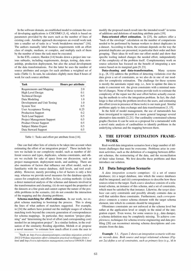
cope with the structural violations in an integration scenario, thatform the base for the following effort calculation. It ships withten such cleaning tasks listed in Table 4; one per type of violation,e.g., of a not-null constraint, and expected result quality (low orhigh). The structure conflict detector can automatically select ex-actly those tasks that the integration practitioner has to perform inthe data integration scenario to fix structural violations.
However, simply designating a task for each given violation isnot sufficient, as data cleaning operations usually have side effectsthat can cause new violations. For instance, the structure conflictdetector reveals that there are 102 artists in the source data that haveno albums and can thus not be represented in the target schema.
5Among competing hypotheses, the one with the fewest as-sumptions should be selected.
67
Result qualityConstraint Low effort High quality
Not null violated Reject tuple Add missing valueUnique violated Set values to null Aggregate tuplesMultiple attribute Keep any value Merge values
valuesValue w/o Drop value Create enclosing
enclosing tuple tupleFK violated Delete dangling Add referenced value
value
Table 4: Structural conflicts and their corresponding cleaning tasks.
The high-quality solution is to apply the task Create tuples for de-tached values, that creates record tuples to store these artists, sothat they do not have to be discarded. These new tuples wouldviolate the not-null constraint on the title attribute, though, so sub-sequent cleaning tasks are necessary. To account for such impacts,we simulate applied cleaning tasks on virtual CSG instances as ex-emplified in Figure 5. In addition to the prescribed cardinalities, thetarget CSG is annotated with actual cardinalities. In contrast to theprescribed cardinalities, those do not prescribe schema constraintsbut describe the state of the (conceptually) integrated source data –in terms of its relationships’ cardinalities. Hence, the actual cardi-nalities are initialized with the inferred cardinalities from the sourcedatabase. Figure 5a depicts this initial state. As long as there areactual cardinalities (on the left-hand side) that are not subsets ofthe prescribed ones, the CSG instance is invalid wrt. its constraints.Now, if the structure repair planner has chosen a cleaning task, e.g.,adding new records tuples for artists without albums, its (side) ef-fects are simulated by modifying the actual cardinalities, as shownin Figure 5b with bold print. So, amongst others the actual cardi-nality of artist ! records is changed from 0..⇤ to 1..⇤, reflectingthat all artists appear in a record after the task, and the cardinality ofrecords ! title is altered from 1 to 0..1, stating that some recordswould then have no title. The latter forms a new constraint viola-tion. Now, a successive repair task can be applied on this alteredCSG instance, e.g., the task Add missing values, which leads to thestate of Figure 5c.
records
artist title gen1..*⊈1 1⊆1
0..*⊈1..* 1..*⊆1..*
(a) Initial state.
!
records
artist title gen1..*⊈1 0..1⊈1
1..*⊆1..* 1..*⊆1..*
(b) State after Add newtuples for records.
!
records
artist title gen1..*⊈1 1⊆1
1..*⊆1..* 1..*⊆1..*
(c) State after Add miss-ing values for title.
Figure 5: Extract of a virtual CSG instance as cleaning tasks areperformed on it.
This procedure of picking a task and simulating its effects is re-peated until the virtual CSG instance contains no more violations.Furthermore, the structure repair planner orders the repair tasks, sothat tasks that cause new structural violations (or might break an al-ready fixed violation) precede the task that fixes this violation. Thisis not computationally expensive, because we need to order onlytasks that affect a common relationship, but doing so allows for thedetection of “infinite cleaning loops”, where the execution orderof cleaning tasks forms a cycle. In most cases, these cycles area consequence of contradicting repair tasks. EFES proposes only
consistent repair strategies. Additionally, the knowledge of the nec-essary cleaning tasks in a data integration scenario, including theirorder, are a valuable aid that can positively impact the integrationeffort spent on coping with structural conflicts. Therefore, the or-dered task list is provided to the user. Finally, the determined clean-ing tasks are fed into the user-defined effort calculation functions,which automatically determine the effort for dealing with structuralviolations in the given scenario. Table 5 presents this effort for theexample scenario.
Task Repetitions EffortAdd tuples (records) 102 5 minsAdd missing values (title) 102 204 minsMerge values (title) 503 15 mins
Total 224 mins
Table 5: High-quality structure repair tasks and their estimated ef-fort using the effort calculation functions from Table 9.
5. VALUE HETEROGENEITIESValue heterogeneities are a frequent class of data integration
problems with a common factor: corresponding attributes in thesource and target schema use different representations for their val-ues. For instance, in Example 3.3 the target table tracks stores songdurations as strings, whereas the source table songs stores thesedurations in milliseconds as integers. An integration practitionermight therefore want to convert or discard the source values toavoid having different value representations in the tracks.durationattribute. Thus, value heterogeneities can increase the integrationeffort.
This section presents a module in EFES to estimate the effortcaused by value heterogeneities. The data complexity is computedby the value fit detector, which analyzes the source and target datato detect different types of value heterogeneities between them.These heterogeneities are then reported to the value transforma-tion planner, the task model that proposes data cleaning tasks inresponse to the heterogeneity issues. Finally, the effort for the pro-posed tasks can be calculated.
5.1 Value Fit DetectorThe basic approach of the value fit detector is to aggregate source
and target data into statistics and compare these statistics to detectheterogeneities. Statistics are eligible for this evaluation, becausethey allow efficient comparison for large amounts of data, whileenabling extensibility (as new functions can be added) and com-pleteness (as issues that are not captured by available metadata canbe discovered). Furthermore, statistics help to detect the especiallymeaningful, general data properties that characterize the data as awhole. In particular, if the source data does not match the observedor specified characteristics of the target dataset, plainly integratingthis source data would impair the overall quality of the integrationresult: integration practitioners might want to spend effort to makesource data consistent with the target data characteristics.
The value fit detector implements this idea as follows: Givenan integration scenario, it processes all pairs of source and targetattributes that are connected by a correspondence. For each suchpair, statistic values of both attributes are calculated, with the targetattribute’s datatype designating which exact statistic types to use.In particular, we consider the following statistics:
• The fill status counts the null values in an attribute and the
68

values that cannot be cast to the target attribute’s datatype.
• The constancy is the inverse of Shannon’s information en-tropy and is useful to classify whether the values of an at-tribute come from a discrete domain [17].
• The text pattern statistic collects frequent patterns in a stringattribute.
• Character histogram captures the relative occurrences ofcharacters in a string attribute.
• The string length statistic determines the average stringlength and its standard deviation for a string attribute.
• Similarly, the mean statistic collects the mean value and stan-dard deviation of a numeric attribute.
• The histogram statistic describes numeric attributes as his-tograms.
• Value ranges are used to determine the minimum and maxi-mum value of a numeric attribute.
• For attributes with values from a discrete domain, the top-kvalues statistic identifies the most frequent values.
For Example 3.3, the string-typed duration target attribute des-ignates the fill status, the text pattern statistic, the character his-togram, the string length statistic, and the top-k values as interest-ing statistics to be collected.
In the next step, a decision model identifies, based on the gath-ered statistics values, the different types of value heterogeneitieswithin the inspected attribute pair. Algorithm 1 outlines this de-cision model, which consists of a sequence of rules. The evalua-tion of each rule has its own, mostly simple, logic. The first rule(substantiallyFewerSourceValues), for instance, is evaluated bycomparing the fill status statistics of the source and target attribute.
Algorithm 1: Detect value heterogeneities.Data: source attribute statistics Ss, target attribute statistics St
Result: value heterogeneities V1 if substantiallyFewerSourceValues(Ss,St) then2 add Too few source elements to V ;
3 if hasIncompatibleValues(Ss) then4 add Different value representations (critical) to V ;
5 if domainRestricted(Ss) ^ ¬domainRestricted(St) then6 add Too coarse-grained source values to V ;7 else if ¬domainRestricted(Ss) ^ domainRestricted(St) then8 add Too fine-grained source values to V ;9 else if domainSpecificDifferences(Ss,St) then
10 add Different value representations to V ;
For the above example attribute pair, the fill-statuses are for bothattributes near 100 %, there are no incompatible source values (in-tegers can always be cast to strings), and neither of the attributesis domain-restricted. Still, possible domain-specific differences be-tween them might be present. The evaluation of this last rule ismore complex. For this purpose, a set of statistics, that are spe-cific to the target attribute’s datatype, are computed, e.g., the stringformat and string length statistic for the string-typed, not domain-restricted duration attribute. To compare these statistics among at-tributes, for each of them of type ⌧ , an importance score i
�St(⌧)
�
and a fit value f�Ss(⌧),St(⌧)
�are calculated. These calculations
are specific to the actual statistics. Intentionally, the importancescore describes how important the statistic type at hand is for thetarget attribute. For example, in the duration attribute, all valueshave the same text pattern [number ":" number], so the string for-mat statistic is presumably an important characteristic and shouldtherefore have a high importance score. If it had many different textpatterns in contrast, its importance would be close to 0. In addition,the fit value measures to what extent the source attribute statistics fitinto the target attribute statistics. For instance, the length attributeprovides only values with the differing pattern [number] leading toa low fit value. Eventually, the fit values for all applied statistictypes are averaged using the importance scores as weights:
fdef=
X
⌧
⇣i�St(⌧)
�· f
�Ss(⌧),St(⌧)
�⌘
This overall fit value tells to what extent the source attribute fulfillsthe most important characteristics of the target attribute. If it fallsbelow a certain threshold, we assume domain-specific differencesin between the compared attributes and Algorithm 1 issues an ac-cording value heterogeneity, e.g., Different value representationsbetween the attributes length and duration. In experiments withimportance scores and fit values between 0 and 1, we found 0.9to be a good threshold to separate seamlessly integrating attributepairs from those that had notably different characteristics.
The set of all value heterogeneities for all attribute pairs formsthe complexity report of the value fit detector that can in the fol-lowing be processed by the value transformation planner. Table 6shows the complexity report for the example scenario. Note thatthe value heterogeneities can carry additional information that arederived from the attribute statistics as well and that can be usefulto produce accurate estimates. These parameters are not furtherdescribed in this paper.
Value heterogeneity Additional parametersDifferent value representation 274.523 source values,
(length ! duration) 260.923 distinct source values
Table 6: Complexity report of the value fit detector.
5.2 Value Transformation PlannerThe value transformation planner proposes tasks to solve value
heterogeneities as specified in Table 7. In contrast to the struc-ture repair tasks from Section 4.2, those tasks do not have interde-pendencies. Therefore, the value transformation planner can sim-ply propose an appropriate task for each given value heterogeneitybased on the expected result quality of the data integration. For thefour different types of value heterogeneities, there are only five dif-ferent tasks, because for a low-effort integration result, value het-erogeneities can in most cases be simply ignored. So, the Differentvalue representations between the duration and length attributesmight either be neglected (leading to no additional effort) or, for ahigh-quality integration result, the value fit detector issues the taskConvert values. This task is then again fed into the effort calcula-tion functions that compute the effort that is necessary for the taskcompletion. Table 8 illustrates the resulting effort estimate.
6. EXPERIMENTSTo show the viability of the general effort estimation architec-
ture and its different models, we conducted experiments with real-world data from two different domains. In the following, we firstintroduce the system and its configuration. We then describe the
69
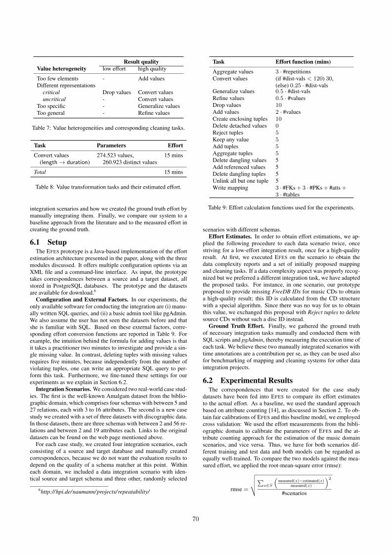
Result qualityValue heterogeneity low effort high quality
Too few elements - Add valuesDifferent representations
critical Drop values Convert valuesuncritical - Convert values
Too specific - Generalize valuesToo general - Refine values
Table 7: Value heterogeneities and corresponding cleaning tasks.
Task Parameters EffortConvert values 274.523 values, 15 mins
(length ! duration) 260.923 distinct values
Total 15 mins
Table 8: Value transformation tasks and their estimated effort.
integration scenarios and how we created the ground truth effort bymanually integrating them. Finally, we compare our system to abaseline approach from the literature and to the measured effort increating the ground truth.
6.1 SetupThe EFES prototype is a Java-based implementation of the effort
estimation architecture presented in the paper, along with the threemodules discussed. It offers multiple configuration options via anXML file and a command-line interface. As input, the prototypetakes correspondences between a source and a target dataset, allstored in PostgreSQL databases. The prototype and the datasetsare available for download.6
Configuration and External Factors. In our experiments, theonly available software for conducting the integration are (i) manu-ally written SQL queries, and (ii) a basic admin tool like pgAdmin.We also assume the user has not seen the datasets before and thatshe is familiar with SQL. Based on these external factors, corre-sponding effort conversion functions are reported in Table 9. Forexample, the intuition behind the formula for adding values is thatit takes a practitioner two minutes to investigate and provide a sin-gle missing value. In contrast, deleting tuples with missing valuesrequires five minutes, because independently from the number ofviolating tuples, one can write an appropriate SQL query to per-form this task. Furthermore, we fine-tuned these settings for ourexperiments as we explain in Section 6.2.
Integration Scenarios. We considered two real-world case stud-ies. The first is the well-known Amalgam dataset from the biblio-graphic domain, which comprises four schemas with between 5 and27 relations, each with 3 to 16 attributes. The second is a new casestudy we created with a set of three datasets with discographic data.In those datasets, there are three schemas with between 2 and 56 re-lations and between 2 and 19 attributes each. Links to the originaldatasets can be found on the web page mentioned above.
For each case study, we created four integration scenarios, eachconsisting of a source and target database and manually createdcorrespondences, because we do not want the evaluation results todepend on the quality of a schema matcher at this point. Withineach domain, we included a data integration scenario with iden-tical source and target schema and three other, randomly selected
6http://hpi.de/naumann/projects/ repeatability/
Task Effort function (mins)Aggregate values 3 · #repetitionsConvert values (if #dist-vals < 120) 30,
(else) 0.25 · #dist-valsGeneralize values 0.5 · #dist-valsRefine values 0.5 · #valuesDrop values 10
Add values 2 · #valuesCreate enclosing tuples 10
Delete detached values 0
Reject tuples 5
Keep any value 5
Add tuples 5
Aggregate tuples 5
Delete dangling values 5Add referenced values 5Delete dangling tuples 5Unlink all but one tuple 5Write mapping 3 · #FKs + 3 · #PKs + #atts +
3 · #tables
Table 9: Effort calculation functions used for the experiments.
scenarios with different schemas.Effort Estimates. In order to obtain effort estimations, we ap-
plied the following procedure to each data scenario twice, oncestriving for a low-effort integration result, once for a high-qualityresult. At first, we executed EFES on the scenario to obtain thedata complexity reports and a set of initially proposed mappingand cleaning tasks. If a data complexity aspect was properly recog-nized but we preferred a different integration task, we have adaptedthe proposed tasks. For instance, in one scenario, our prototypeproposed to provide missing FreeDB IDs for music CDs to obtaina high-quality result; this ID is calculated from the CD structurewith a special algorithm. Since there was no way for us to obtainthis value, we exchanged this proposal with Reject tuples to deletesource CDs without such a disc ID instead.
Ground Truth Effort. Finally, we gathered the ground truthof necessary integration tasks manually and conducted them withSQL scripts and pgAdmin, thereby measuring the execution time ofeach task. We believe these two manually integrated scenarios withtime annotations are a contribution per se, as they can be used alsofor benchmarking of mapping and cleaning systems for other dataintegration projects.
6.2 Experimental ResultsThe correspondences that were created for the case study
datasets have been fed into EFES to compare its effort estimatesto the actual effort. As a baseline, we used the standard approachbased on attribute counting [14], as discussed in Section 2. To ob-tain fair calibrations of EFES and this baseline model, we employedcross validation: We used the effort measurements from the bibli-ographic domain to calibrate the parameters of EFES and the at-tribute counting approach for the estimation of the music domainscenarios, and vice versa. Thus, we have for both scenarios dif-ferent training and test data and both models can be regarded asequally well-trained. To compare the two models against the mea-sured effort, we applied the root-mean-square error (rmse):
rmse =
vuutP
s2S
⇣measured(s)�estimated(s)
measured(s)
⌘2
#scenarios
70

0
50
100
150
200
250
300
350
Efes
Mea
sure
d
Co
un
tin
g
Efes
Mea
sure
d
Co
un
tin
g
Efes
Mea
sure
d
Co
un
tin
g
Efes
Mea
sure
d
Co
un
tin
g
Efes
Mea
sure
d
Co
un
tin
g
Efes
Mea
sure
d
Co
un
tin
g
Efes
Mea
sure
d
Co
un
tin
g
Efes
Mea
sure
d
Co
un
tin
g
s1-s2 (low eff.) s1-s2 (high qual.) s1-s3 (low eff.) s1-s3 (high qual.) s3-s4 (low eff.) s3-s4 (high qual.) s4-s4 (low eff.) s4-s4 (highqual.)
Effo
rt [
min
]
Mapping Cleaning Cleaning (Values) Cleaning (Structure)
Figure 6: Effort estimates (EFES), actual effort (Measured), and baseline estimates (Counting) of the Bibliographic scenario.
where S is a set of integration scenarios.We start our analysis with the Amalgam dataset with the results
reported in Figure 6. EFES consistently outperforms the countingapproach in all scenarios. This is explained by the fact that the base-line has no concept of heterogeneity between values in the datasets,but it is one of the main complexity drivers in these integration sce-narios. In terms of the root-mean-square error, EFES achieves 0.47,while the baseline obtains 1.90 (lower values indicates better esti-mations), thus there is an improvement in the effort estimation by afactor of four. Moreover, EFES not only provides the total numberof minutes, but also a detailed break down of where the effort is tobe expected. This turned out to be particular useful to revise theeffort estimate as described above, thus enriching the estimationprocess with further input. In fact, it makes a significant differenceif an integration practitioner has to add hundreds of missing valuesor if tuples with missing values are dropped. The baseline approachalso distinguishes between mapping and cleaning efforts, but it re-lates them neither to integration problems nor actual tasks. Thes4-s4 scenario demonstrates this: source and target database havethe same schema and similar data, so there are no heterogeneitiesto deal with. While we can detect this, the counting approach esti-mates considerable cleaning effort.
When we move to the music datasets, the results in Figure 7show a smaller difference between the two estimation approaches.In fact, EFES outperforms the baseline four times, in three casesbaseline does a better job, and in one case the estimate is basicallythe same. The explanation is that in this domain, there are fewerproblems at the data level and the effort is dominated by the map-ping, which strongly depends on the schema. However, when welook at the root-mean-square error, EFES achieves 1.05, while thebaseline obtains 1.64. Therefore, even in cases where EFES cannotexploit all of its modules, and when counting should perform at itsbest, our systematic estimation is better.
It is important to consider the generality of the presented com-parison. The two case studies are based on real-world data sets withdifferent complexity and quality. When putting the results over theeight scenarios together, EFES achieves a root-mean-square error of0.84, while the baseline obtains 1.70. In terms of execution time,EFES relies on simple SQL queries only for the analysis of the dataand completes within seconds for databases with thousands of tu-ples. This overhead can be neglected in the context of the dominat-
ing integration cost.
7. CONCLUSIONSWe have tackled the problem of estimating the complexity and
the effort for data integration scenarios. As data integration iscomposed of many different activities, we proposed a novel sys-tem, EFES, that integrates different ad-hoc estimation modules ina unified fashion. We have introduced three modules that takecare of estimating the complexity and effort of (i) mapping activi-ties, (ii) cleaning of structural conflicts arising because of differentstructures and integrity constraints, and (iii) resolving heterogene-ity in integrated data, such as different formats. Experimental re-sults show that our system outperforms the standard baseline up toa factor of four in terms of precision of the estimated effort time inminutes. When compared to the effective time required by a humanto achieve integration, EFES provides a close estimate for most ofthe cases.
We believe that our work is only a first step in this challengingproblem. One possible general direction is to integrate EFES withapproaches that measure the benefit of the integration, such as themarginal gain [9]. This integration would allow to plot cost-benefitgraphs for the integration: the more effort, the better the quality ofthe result.
A rather technical challenge in our system is to drop the as-sumption that correspondences among schemas are given. In prac-tice, the effort for creating quality correspondences cannot be com-pletely neglected – although, in our experience it takes considerablyless time than other integration activities – and automatically gener-ated correspondences introduce uncertainty wrt. the produced esti-mates. The accuracy measure as proposed Melnik et al. [19] seemsto be a good starting point to tackle this issue.Acknowledgments. We would like to thank ElKindi Rezig forvaluable discussions in the initial phase of this project.
8. REFERENCES[1] B. Alexe, W.-C. Tan, and Y. Velegrakis. STBenchmark:
towards a benchmark for mapping systems. Proceedings ofthe VLDB Endowment, 1(1):230–244, Aug. 2008.
[2] P. Atzeni, G. Gianforme, and P. Cappellari. A universalmetamodel and its dictionary. In Transactions on
71

0
40
80
120
160
200
Efes
Mea
sure
d
Co
un
tin
g
Efes
Mea
sure
d
Co
un
tin
g
Efes
Mea
sure
d
Co
un
tin
g
Efes
Mea
sure
d
Co
un
tin
g
Efes
Mea
sure
d
Co
un
tin
g
Efes
Mea
sure
d
Co
un
tin
g
Efes
Mea
sure
d
Co
un
tin
g
Efes
Mea
sure
d
Co
un
tin
g
f1-m2 (low eff.) f1-m2 (high qual.) m1-d2 (low eff.) m1-d2 (high qual.) m1-f2 (low eff.) m1-f2 (high qual.) d1-d2 (low eff.) d1-d2 (highqual.)
Effo
rt [
min
]
Cleaning (Structure) Cleaning (Values) Cleaning Mapping
Figure 7: Effort estimates (Efes), actual effort (Measured), and baseline estimates (Counting) of the Music scenario.
Large-Scale Data-and Knowledge-Centered Systems I, pages38–62. Springer, 2009.
[3] B. Boehm. Software Engineering Economics. Prentice-Hall,Englewood Cliffs, NJ, 1981.
[4] B. Boehm, C. Abts, A. W. Brown, S. Chulani, B. K. Clark,E. Horowitz, R. Madachy, D. J. Reifer, and B. Steece.Software Cost Estimation with COCOMO II. Prentice-Hall,Englewood Cliffs, NJ, 2000.
[5] A. Calì, D. Calvanese, G. De Giacomo, and M. Lenzerini.Data integration under integrity constraints. InformationSystems, 29(2):147–163, 2004.
[6] A. Calì, G. Gottlob, and T. Lukasiewicz. A generaldatalog-based framework for tractable query answering overontologies. In Proceedings of the Symposium on Principlesof Database Systems (PODS), pages 77–86, 2009.
[7] M. P. Consens, I. F. Cruz, and A. O. Mendelzon. Visualizingqueries and querying visualizations. SIGMOD Record,21(1):39–46, 1992.
[8] M. Dallachiesa, A. Ebaid, A. Eldawy, A. Elmagarmid,I. Ilyas, M. Ouzzani, and N. Tang. Towards a commoditydata cleaning system. In Proceedings of the InternationalConference on Management of Data (SIGMOD), pages541–552, 2013.
[9] X. L. Dong, B. Saha, and D. Srivastava. Less is more:Selecting sources wisely for integration. Proceedings of theVLDB Endowment, 6(2):37–48, 2012.
[10] J. Euzenat and P. Shvaiko. Ontology matching.Springer-Verlag, Heidelberg (DE), 2nd edition, 2013.
[11] R. Fagin, P. G. Kolaitis, R. J. Miller, and L. Popa. Dataexchange: Semantics and query answering. In Proceedingsof the International Conference on Database Theory (ICDT),pages 207–224, Siena, Italy, 2003.
[12] R. Fagin, P. G. Kolaitis, L. Popa, and W. C. Tan:. Composingschema mappings: Second-order dependencies to the rescue.In Proceedings of the Symposium on Principles of DatabaseSystems (PODS), pages 83–94, Paris, France, 2004.
[13] F. Geerts, G. Mecca, P. Papotti, and D. Santoro. Mapping andCleaning. In Proceedings of the International Conference onData Engineering (ICDE), pages 232–243, 2014.
[14] B. Harden. Estimating extract, transform, and load (ETL)projects. Technical report, Project Management Institute,2010.
[15] S. Kandel, A. Paepcke, J. Hellerstein, and J. Heer. Wrangler:interactive visual specification of data transformation scripts.In CHI, pages 3363–3372, 2011.
[16] A. Kumar P, S. Narayanan, and V. M. Siddaiah. COTSintegrations: Effort estimation best practices. In ComputerSoftware and Applications Conference Workshops, 2010.
[17] D. MacKay. Information Theory, Inference, and LearningAlgorithms. Cambridge University Press, 2003.
[18] B. Marnette, G. Mecca, P. Papotti, S. Raunich, andD. Santoro. ++Spicy: an opensource tool forsecond-generation schema mapping and data exchange.Proceedings of the VLDB Endowment, 4(12):1438–1441,2011.
[19] S. Melnik, H. Garcia-Molina, and E. Rahm. Similarityflooding: A versatile graph matching algorithm. InProceedings of the International Conference on DataEngineering (ICDE), pages 117–128, 2002.
[20] F. Naumann. Data profiling revisited. SIGMOD Record,42(4):40–49, 2013.
[21] P. Papotti and R. Torlone. Schema exchange: Genericmappings for transforming data and metadata. Data &Knowledge Engineering (DKE), 68(7):665–682, 2009.
[22] E. Rahm and H. H. Do. Data cleaning: Problems and currentapproaches. IEEE Data Engineering Bulletin, 23(4):3–13,2000.
[23] T. Rekatsinas, X. L. Dong, L. Getoor, and D. Srivastava.Finding quality in quantity: The challenge of discoveringvaluable sources for integration. In Proceedings of theConference on Innovative Data Systems Research (CIDR),2015.
[24] K. P. Smith, M. Morse, P. Mork, M. H. Li, A. Rosenthal,M. D. Allen, and L. Seligman. The role of schema matchingin large enterprises. In Proceedings of the Conference onInnovative Data Systems Research (CIDR), 2009.
[25] J. Wang, T. Kraska, M. J. Franklin, and J. Feng. CrowdER:Crowdsourcing entity resolution. Proceedings of the VLDBEndowment, 5(11):1483–1494, 2012.
72