Online Appendix to “Estimating Demand forDifferentiated Products with Zeroes in Market Share

Data”

In this online appendix, we introduce the profiling approach for models defined by many moment

inequalities. The profiling approach developed here is similar to the penalized resampling approach

in Bugni, Canay, and Shi (2016) for unconditional moment inequality models.18 Section D describes

the profiling approach and gives the formal results, and Section E presents the proofs of those results.

D The Profiling Approach

The profiling approach applies to general moment inequality models with many moment inequali-

ties. Thus from this point on, we focus on the moment inequality model:

Eρ(wt, θ, g) ≥ 0 for all g ∈ G, (D.1)

where ρ takes values in Rk. We also let G be a general set of indices that can be either countable

or uncontable. Let µ : G → [0, 1] denote a probability density on G. We assume the data wtTt=1 are

i.i.d. across t.

We assume that there is a parameter of interest, γ0, that is related to θ0 through:

γ0 ∈ Γ(θ0) ⊆ Rdγ , (D.2)

where Γ : Θ → 2Rdγ

is a known mapping where 2Rdγ

denotes the collection of all subsets of Rdγ .

Three examples of Γ are given below:

Example. Γ(θ) = α: γ0 is the price coefficient α0. In the simple logit model, the price coefficient

is all one needs to know to compute the demand elasticity.

Example. Γ(θ) = ej(p, π, θ, x) = (αpj/πj)(∂σj(σ−1(π, x, λ), x, λ)/∂δj): γ0 is the own-price de-

mand elasticity of product j at a given value of the price vector p, the choice probability vector π

and the covariates x.

Example. Γ(θ) = ej(p, π, θ, x) : π ∈ [πl, πu]: γ0 is the demand elasticity of product j at a given

value of the price vector p, the covariates x and at the choice probability vector that is known to lie

between πl and πu. This example is particularly useful when the elasticity depends on the choice

probability but the choice probability is only known to lie in an interval.

18The profiling approach here, made public in the 2013 version of this paper, was developed before that in Bugni,Canay, and Shi (2016).

40

Let Γ0 be the identified set of γ0: Γ0 = γ ∈ Rdγ : ∃θ ∈ Θ0 s.t. Γ(θ) 3 γ, where Θ0 = θ ∈ Θ :

Eρ(wt, θ, g) ≥ 0 ∀g ∈ G. The profiling approach constructs a confidence set for γ0 by inverting a

test of the hypothesis:

H0 : γ ∈ Γ0, (D.3)

for each parameter value γ. The confidence set is the collection of values that are not rejected by

the test.

Let Γ−1(γ) = θ ∈ Θ : Γ(θ) 3 γ. The test to be inverted uses the profiled test statistic:

TT (γ) = T × minθ∈Γ−1(γ)

QT (θ), (D.4)

where QT (θ) is an empirical measure of the violation to the moment inequalities. The confidence

set of confidence level p is the set of all points for which the test statistic does not exceed a critical

value cT (γ, p):

CST = γ ∈ Rdγ : TT (γ) ≤ cT (γ, p). (D.5)

Notice that the new confidence set only involves computing a dγ-dimensional level set, where dγ is

often 1. The profiling transfers the burden of searching (for low values) over the surface of the non

smooth function T (θ)− c(θ) to searching over the surface of the typically smooth and often convex

function QT (θ).

We choose a critical value, cT (γ, p), of significance level 1− p ∈ (0, 0.5), to satisfy

limT→∞

inf(γ,F )∈H0

Pr F (TT (γ) > cT (γ, p)) ≤ 1− p, (D.6)

where F is the distribution on (wt)Tt=1 and H0 is the null parameter space of (γ, F ). The definition

of H0 along with other technical assumptions are given in Section D.4.19

As a result of (D.6), the confidence set asymptotically has the correct minimum coverage prob-

ability:

lim infT→∞

inf(γ,F )∈H0

PrF (γ ∈ CST ) ≥ p. (D.7)

The left hand side is called the “asymptotic size” of the confidence set in Andrews and Shi (2013).

We achieve the asymptotic size control by deriving an asymptotic approximation for the distribution

of the profiled test statistic TT (γ) that is uniformly valid over (γ, F ) ∈ H0 and simulating the

critical value from the approximating distribution through either a subsampling or a bootstrapping

procedure.

In the next subsections, we describe the test statistic and the critical value in detail and show

19Note that we use F to denote the distribution of the full observed data vector and thus (γ, F ) captures everything

unknown in the expression PrF (TT (γ) > cT (γ, p)). This notation differs from the traditional literature where the truedistribution of the data is often indicated by the true value of θ, but is standard in the recent partial identificationliterature. See Romano and Shaikh (2008) and Andrews and Shi (2013).

41

that (D.7) holds.

D.1 Test Statistic

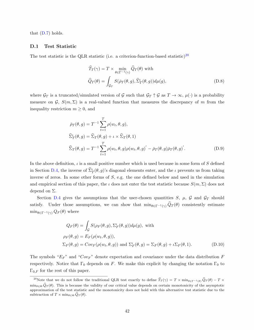
The test statistic is the QLR statistic (i.e. a criterion-function-based statistic)20

TT (γ) = T × minθ∈Γ−1(γ)

QT (θ) with

QT (θ) =

∫GTS(ρT (θ, g), Σι

T (θ, g))dµ(g), (D.8)

where GT is a truncated/simulated version of G such that GT ↑ G as T → ∞, µ(·) is a probability

measure on G, S(m,Σ) is a real-valued function that measures the discrepancy of m from the

inequality restriction m ≥ 0, and

ρT (θ, g) = T−1T∑t=1

ρ(wt, θ, g),

ΣιT (θ, g) = ΣT (θ, g) + ι× ΣT (θ, 1)

ΣT (θ, g) = T−1T∑t=1

ρ(wt, θ, g)ρ(wt, θ, g)′ − ρT (θ, g)ρT (θ, g)

′. (D.9)

In the above definition, ι is a small positive number which is used because in some form of S defined

in Section D.4, the inverse of ΣιT (θ, g)’s diagonal elements enter, and the ι prevents us from taking

inverse of zeros. In some other forms of S, e.g. the one defined below and used in the simulation

and empirical section of this paper, the ι does not enter the test statistic because S(m,Σ) does not

depend on Σ.

Section D.4 gives the assumptions that the user-chosen quantities S, µ, G and GT should

satisfy. Under those assumptions, we can show that minθ∈Γ−1(γ) QT (θ) consistently estimate

minθ∈Γ−1(γ)QF (θ) where

QF (θ) =

∫GS(ρF (θ, g),Σι

F (θ, g))dµ(g), with

ρF (θ, g) = EF (ρ(wt, θ, g)),

ΣF (θ, g) = CovF (ρ(wt, θ, g)) and ΣιF (θ, g) = ΣF (θ, g) + ιΣF (θ, 1). (D.10)

The symbols “EF ” and “CovF ” denote expectation and covariance under the data distribution F

respectively. Notice that Γ0 depends on F . We make this explicit by changing the notation Γ0 to

Γ0,F for the rest of this paper.

20Note that we do not follow the traditional QLR test exactly to define TT (γ) = T × minθ∈Γ−1(θ) QT (θ) − T ×minθ∈Θ QT (θ). This is because the validity of our critical value depends on certain monotonicity of the asymptoticapproximation of the test statistic and the monotonicity does not hold with this alternative test statistic due to thesubtraction of T ×minθ∈Θ QT (θ).

42

We can also show that minθ∈Γ−1(γ)QF (θ) = 0 if and only if γ ∈ Γ0,F . This result combined

with the consistency of minθ∈Γ−1(γ) QT (θ) implies that TT (γ) diverges to infinity at γ /∈ Γ0,F . That

implies that there is no information loss in using such a test statistic. Lemma D.1 summarizes those

two results. The parameter space H of (γ, F ) appearing in the lemma is defined in Assumption

D.2 in Section D.4.

Lemma D.1. Suppose that Assumptions D.1, D.2, D.4, D.5(a), and D.6(a) and (d) hold. Then for

any (γ, F ) ∈ H,

(a) minθ∈Γ−1(γ) QT (θ)→p minθ∈Γ−1(γ)QF (θ) under F , and

(b) minθ∈Γ−1(γ)QF (θ) ≥ 0 and = 0 if and only if γ ∈ Γ0,F .

In the simulation and the empirical application of this paper, the following choices of S, G, GT and µ

are used mainly for computational convenience. For G, we use the one defined in (4.19). For GT ,

the truncated version of G, we define it to be the same as G except that we let r run from r0 to rT

where rT →∞ as T →∞ in the definition.

For S , we use

S(m,Σ) =k∑j=1

[mj ]2−, (D.11)

where mj is the jth coordinate of m and [x]− = |minx, 0|. There may be efficiency loss from not

weighting the moments using the variance matrix, but this S function brings great computational

convenience because it makes the minimization problem in (D.4) a convex one. For µ(·), we use

µ(ga,r,ζ) ∝ (100 + r)−2(2r)−dzcK−1d for g ∈ Gd,cc, (D.12)

where Kd is the number of elements in Zd. The same µ measure is used and seems to work well in

Andrews and Shi (2013).

D.2 Critical Value

We propose two types of critical values, one based on standard subsampling and the other based

on a bootstrapping procedure with moment shrinking. Both are simple to compute. The bootstrap

critical value may have better small sample properties, and is the procedure we use in the empirical

section.21 It is worth noting that we resample at the market level for both the subsampling and

the bootstrap.

Let us formally define the subsampling critical value first. It is obtained through the standard

subsampling steps: [1] from 1, ..., T, draw without replacement a subsample of market indices

of size bT ; [2] compute TT,bT (γ) in the same way as TT (γ) except using the subsample of markets

corresponding to the indices drawn in [1] rather than the original sample; [3] repeat [1]-[2] ST times

obtain ST independent (conditional on the original sample) copies of TT,bT (γ); [4] let c∗sub (γ, p) be

21The bootstrap procedure here, like in most problems with partial identification, does not lead to higher-orderimprovement.

43

the p quantile of the ST independent copies. Let the subsampling critical value be

csubT (γ, p) = c∗sub (γ, p+ η∗) + η∗, (D.13)

where η∗ > 0 is an infinitesimal number. The infinitesimal number is used to avoid making hard-

to-verify uniform continuity and strict monotonicity assumptions on the distribution of the test

statistic. It can be set to zero if one is willing to make the continuity assumptions. Such infinitesimal

numbers are also employed in Andrews and Shi (2013). One can follow their suggestion of using

η∗ = 10−6.

Let us now define the bootstrap critical value. It is obtained through the following steps: [1]

from the original sample 1, ..., T, draw with replacement a bootstrap sample of size T ; denote

the bootstrap sample by t1, ..., tT , [2] let the bootstrap statistic be

T ∗T (γ) = minθ∈Θ:γ∈Γ(θ)

∫GS(ν∗T (θ, g) + κ

1/2T ρT (θ, g), Σι

T (θ, g))dµ(G), , (D.14)

where ν∗T (θ, g) =√T (ρ∗T (θ, g) − ρT (θ, g)), ρ∗T (θ, g) = T−1

∑Tτ=1 ρ(Xtτ , θ, g), and κT is a sequence

of moment shrinking parameters: κT /T + κ−1T → 0; [3] repeat [1]-[2] ST times and obtain ST

independent (conditional on the original sample) copies of T ∗T (γ); [4] let c∗bt(γ, p) be the p quantile

of the ST copies. Let the bootstrap critical value be

cbtT (γ, p) = c∗bt(γ, p+ η∗) + η∗, (D.15)

where η∗ > 0 is an infinitesimal number which has the same function as in the subsampling critical

value above.

Critical values that are not based on resampling are possible, too. For example, one can define

a critical value similar to the bootstrap one, except with ν∗T (θ, g) replaced by a Gaussian process

with covariance kernel that equals the sample covariance of ρ(wt, θ(1), g(1)) and ρ(wt, θ

(2), g(2)) for

(θ(j), g(j)) ∈ Θ× G, j = 1, 2. For lack of space, we do not discuss such critical values in detail.

D.3 Coverage Probability

We show that the confidence sets defined in (D.5) using either csubT (γ, p) and cbtT (γ, p) have asymp-

totically correct coverage probability uniformly over H0 under appropriate assumptions. The as-

sumptions are given in Section D.4.

Theorem D.1. Suppose that Assumptions D.1-D.3 and D.5-D.7 hold, then

(a) (D.7) holds with cT (γ, p) = csubT (γ, p), and

(b) (D.7) holds with cT (γ, p) = cbtT (γ, p).

44

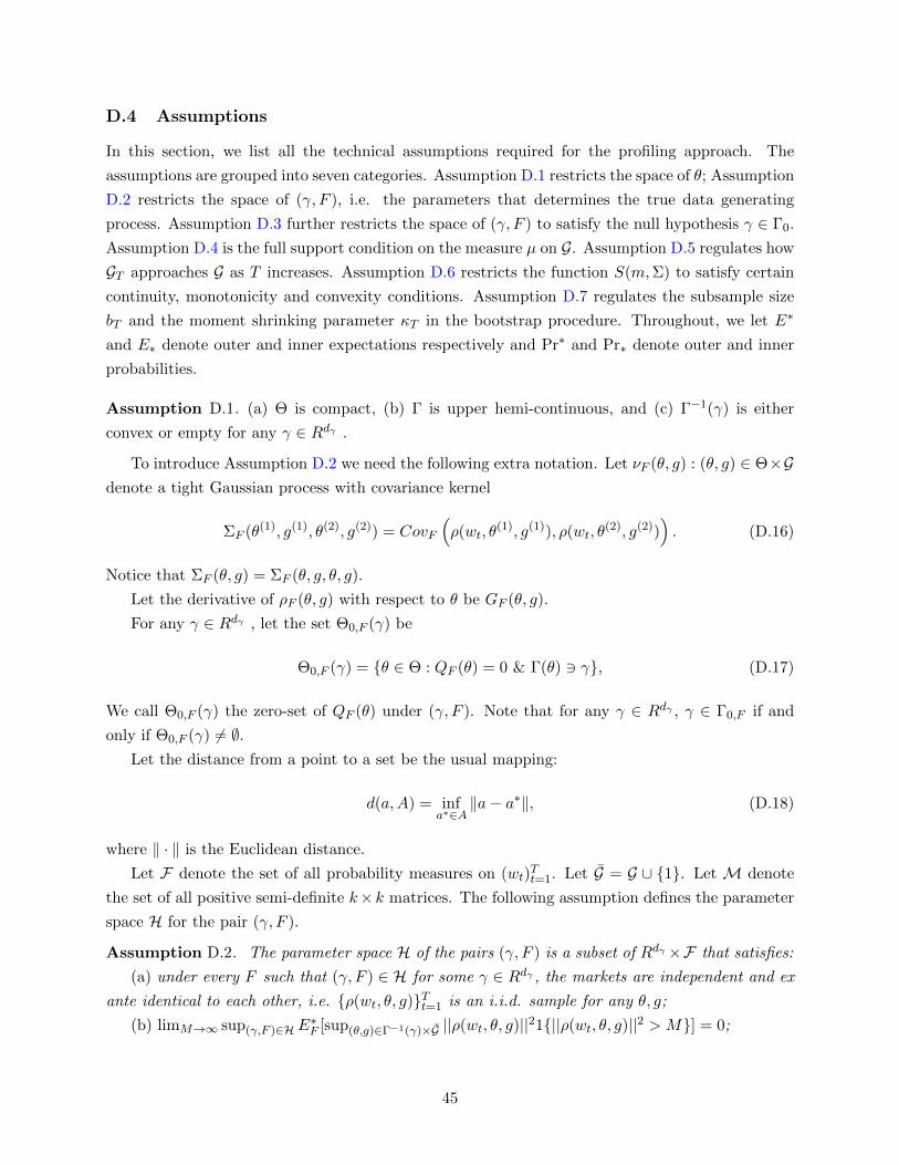
D.4 Assumptions

In this section, we list all the technical assumptions required for the profiling approach. The

assumptions are grouped into seven categories. Assumption D.1 restricts the space of θ; Assumption

D.2 restricts the space of (γ, F ), i.e. the parameters that determines the true data generating

process. Assumption D.3 further restricts the space of (γ, F ) to satisfy the null hypothesis γ ∈ Γ0.

Assumption D.4 is the full support condition on the measure µ on G. Assumption D.5 regulates how

GT approaches G as T increases. Assumption D.6 restricts the function S(m,Σ) to satisfy certain

continuity, monotonicity and convexity conditions. Assumption D.7 regulates the subsample size

bT and the moment shrinking parameter κT in the bootstrap procedure. Throughout, we let E∗

and E∗ denote outer and inner expectations respectively and Pr∗ and Pr∗ denote outer and inner

probabilities.

Assumption D.1. (a) Θ is compact, (b) Γ is upper hemi-continuous, and (c) Γ−1(γ) is either

convex or empty for any γ ∈ Rdγ .

To introduce Assumption D.2 we need the following extra notation. Let νF (θ, g) : (θ, g) ∈ Θ×Gdenote a tight Gaussian process with covariance kernel

ΣF (θ(1), g(1), θ(2), g(2)) = CovF

(ρ(wt, θ

(1), g(1)), ρ(wt, θ(2), g(2))

). (D.16)

Notice that ΣF (θ, g) = ΣF (θ, g, θ, g).

Let the derivative of ρF (θ, g) with respect to θ be GF (θ, g).

For any γ ∈ Rdγ , let the set Θ0,F (γ) be

Θ0,F (γ) = θ ∈ Θ : QF (θ) = 0 & Γ(θ) 3 γ, (D.17)

We call Θ0,F (γ) the zero-set of QF (θ) under (γ, F ). Note that for any γ ∈ Rdγ , γ ∈ Γ0,F if and

only if Θ0,F (γ) 6= ∅.Let the distance from a point to a set be the usual mapping:

d(a,A) = infa∗∈A

‖a− a∗‖, (D.18)

where ‖ · ‖ is the Euclidean distance.

Let F denote the set of all probability measures on (wt)Tt=1. Let G = G ∪ 1. Let M denote

the set of all positive semi-definite k× k matrices. The following assumption defines the parameter

space H for the pair (γ, F ).

Assumption D.2. The parameter space H of the pairs (γ, F ) is a subset of Rdγ ×F that satisfies:

(a) under every F such that (γ, F ) ∈ H for some γ ∈ Rdγ , the markets are independent and ex

ante identical to each other, i.e. ρ(wt, θ, g)Tt=1 is an i.i.d. sample for any θ, g;

(b) limM→∞ sup(γ,F )∈HE∗F [sup(θ,g)∈Γ−1(γ)×G ||ρ(wt, θ, g)||21||ρ(wt, θ, g)||2 > M] = 0;

45

(c) the class of functions ρ(wt, θ, g) : (θ, g) ∈ Γ−1(γ) × G is F -Donsker and pre-Gaussian

uniformly over H;

(d) the class of functions ρ(wt, θ, g)ρ(wt, θ, g)′

: (θ, g) ∈ Γ−1(γ) × G is Glivenko-Cantelli

uniformly over H;

(e) ρF (θ, g) is differentiable with respect to θ ∈ Θ, and there exists constants C and δ1 > 0 such

that, for any (θ(1), θ(2)), sup(γ,F )∈H,g∈G ||vec(GF (θ(1), g))− vec(GF (θ(2), g))|| ≤ C × ||θ(1) − θ(2)||δ1,

and

(f) ΣιF (θ, g) ∈ Ψ for all (γ, F ) ∈ H and θ ∈ Γ−1(γ) where Ψ is a compact subset of M, and

vec(ΣF (·, g(1), ·, g(2))) : (Γ−1(γ))2 → Rk2

: (γ, F ) ∈ H, g(1), g(2) ∈ G are uniformly bounded and

uniformly equicontinuous.

Remark. Part (a) is the i.i.d. assumption, which can be replaced with appropriate weak dependence

conditions at the cost of more complicated derivation in the uniform weak convergence of the

bootstrap empirical process. Part (b) is standard uniform Lindeberg condition. Part (c)-(d) imposes

restrictions on the complexity of the set G as well as on the shape of ρ(wt, θ, g) as a function of

θ. A sufficient condition is (i) ρ(wt, θ, g) is Lipschitz continuous in θ with the Lipschitz coefficient

being integrable and (ii) the set C in the definition of G forms a Vapnik-Cervonenkis set and Jt is

bounded. The Lipschitz continuity is also a sufficient condition of part (f).

The following assumptions defines the null parameter space, H0, for the pair (γ, F ).

Assumption D.3. The null parameter space H0 is a subset of H that satisfies:

(a) for every (γ, F ) ∈ H0, γ ∈ Γ0,F , and

(b) there exists C, c > 0 and 2 ≤ δ2 < 2(δ1 + 1) such that QF (θ) ≥ C · (d(θ,Θ0,F (γ))δ2 ∧ c) for

all (γ, F ) ∈ H0 and θ ∈ Γ−1(γ).

Remark. Part (b) is an identification strength assumption. It requires the criterion function to

increase at certain minimum rate as θ is perturbed away from the identified set. This assumption

is weaker than the quadratic minorant assumption in Chernozhukov, Hong, and Tamer (2007) if

δ2 > 2 and as strong as the latter if δ2 = 2. Putting part (b) and Assumption D.2(e) together,

we can see that there is a trade-off between the minimum identification strength required and

the degree of Hı¿œlder continuity of the first derivative of ρF (·, g). If ρF (·, g) is linear, δ2 can be

arbitrarily large – the criterion function can increase very slowly as θ is perturbed away from the

identified set.

The following assumption is on the measure µ. For any θ, let a pseudo-metric on G be: ||g(1)−g(2)||θ,F = ||ρF,j(θ, g(1))− ρF,j(θ, g(2))||. This assumption is needed for Lemma D.1 and not needed

for the asymptotic size result Theorem D.1.

Assumption D.4. For any θ ∈ Θ, µ(·) has full support on the metric space (G, || · ||θ,F ).

Remark. Assumption D.4 implies that for any θ ∈ Θ, F and j, if ρF,j(θ, g0) < 0 for some g0 ∈ G,

then there exists a neighborhood N (g0) with positive µ-measure such that ρF,j(θ, g) < 0 for all

g ∈ N (g0).

46

The following assumption is on the set GT .

Assumption D.5. (a) GT ↑ G as T →∞ and

(b) lim supT→∞ sup(γ,F )∈H0supθ∈Γ−1(γ)

∫G\GT S(

√TρF (θ, g),ΣF (θ, g))dµ(g) = 0.

The following assumptions are imposed on the function S. For a ξ > 0, let the ξ-expansion of

Ψ be Ψξ = Σ ∈M : infΣ1∈Ψ ||vech(Σ)− vech(Σ1)|| ≤ ξ.

Assumption D.6. (a) S(m,Σ) : (−∞,∞]k ×Ψξ → R is continuous for some ξ > 0.

(b) There exists a constant C > 0 and ξ > 0 such that for any m1,m2 ∈ Rk and Σ1,Σ2 ∈ Ψξ,

we have |S(m1,Σ1) − S(m2,Σ2)| ≤ C√

(S(m1,Σ1) + S(m2,Σ2))(S(m2,Σ2) + 1)∆, where ∆ =

||m1 −m2||2 + ||vech(Σ1 − Σ2)||.(c) S is non-increasing in m.

(d) S(m,Σ) ≥ 0 and S(m,Σ) = 0 if and only if m ∈ [0,∞]k.

(e) S is homogeneous in m of degree 2.

(f) S is convex in m ∈ Rdm for any Σ ∈ Ψξ.

Remark. We show in the lemma below that Assumption D.6 is satisfied by the example in (D.11)

(which is used in our empirical section) as well as the SUM and MAX functions in Andrews and

Shi (2013):

SUM: S(m,Σ) =

k∑j=1

[mj/σj ]2−, and

MAX: S(m,Σ) = max1≤j≤k

[mj/σj ]2−, (D.19)

where σ2j is the jth diagonal element of Σ. Assumptions D.6(b) and (f) rule out the QLR function

in Andrews and Shi (2013): S(m,Σ) = mint≥0(m− t)′Σ−1(m− t).

Lemma D.2. (a) Assumption D.6 is satisfied by the S function in (D.11) for any set Ψ.

(b) Assumption D.6 is satisfied by the SUM and the MAX functions in (D.19) if Ψ is a compact

subset of the set of positive semi-definite matrix with diagonal elements bounded below by some

constant ξ2 > 0.

The following assumptions are imposed on the tuning parameters in the subsampling and the

bootstrap procedures.

Assumption D.7. (a) In the subsampling procedure, b−1T + bTT

−1 → 0 and ST →∞, and

(b)In the bootstrap procedure, κ−1T + κTT

−1 → 0 and ST →∞.

47

D.5 Proof of Lemmas D.1 and D.2

Proof of Lemma D.1. (a) Assumptions D.2(c)-(d) imply that under F ,

∆ρ,T ≡ supθ∈Γ−1(γ),g∈G

||ρT (θ, g)− ρF (θ, g)|| →p 0, and

supθ∈Γ−1(γ),g∈G

||vech(ΣT (θ, g)− ΣF (θ, g))|| →p 0. (D.20)

The second convergence implies that

∆Σ,T ≡ supθ∈Γ−1(γ),g∈G

||vech(ΣιT (θ, g)− Σι

F (θ, g))|| →p 0. (D.21)

By Assumption D.2(b), supθ∈Γ−1(γ),g∈G ||ρF (θ, g)|| < M∗ for someM∗ <∞. Thus, (ρF (θ, g),ΣιF (θ, g)) :

(θ, g) ∈ Γ−1(γ) × G is a subset of the compact set [−M∗,M∗]k × Ψ. By Assumption D.2(f) and

Equations (D.20) and (D.21), we have (ρT (θ, g), ΣιT (θ, g)) : (θ, g) ∈ Γ−1(γ) × G ⊆ [−M∗ −

ξ,M∗ + ξ]k ×Ψξ with probability approaching one for any ξ > 0. By Assumption D.6(a), S(m,Σ)

is uniformly continuous on [−M∗,M∗]k ×Ψ. Therefore, for any ε > 0,

Pr F

(∣∣∣∣ minθ∈Γ−1(γ)

QT (θ)− minθ∈Γ−1(γ)

∫GTS(ρF (θ, g),Σι

F (θ, g))dµ(g)

∣∣∣∣ > ε

)≤Pr F

(sup

θ∈Γ−1(γ),g∈G|S(ρt(θ, g), Σι

t(θ, g))− S(ρF (θ, g),ΣιF (θ, g))| > ε

)→0. (D.22)

Now it is left to show that minθ∈Γ−1(γ)

∫GT S(ρF (θ, g),Σι

F (θ, g))dµ(g)→ minθ∈Γ−1(γ)QF (θ) as T →∞. Observe that

0 ≤ minθ∈Γ−1(γ)

QF (θ)− minθ∈Γ−1(γ)

∫GTS(ρF (θ, g),Σι

F (θ, g))dµ(g)

≤ supθ∈Γ−1(γ)

∫G/GT

S(ρF (θ, g),ΣιF (θ, g))dµ(g)

≤∫G/GT

supθ∈Γ−1(γ)

S(ρF (θ, g),ΣιF (θ, g))dµ(g). (D.23)

We have supθ∈Γ−1(γ) S(ρF (θ, g),ΣιF (θ, g)) < ∞, because ρF (θ, g) ∈ [−M∗,M∗]k and Σι

F (θ, g) ∈ Ψ

and Assumption D.6(a). Thus the last line of (D.23) converges to zero under Assumption D.5(a).

This and (D.22) together show part (a).

(b) The first half of part (b), minθ∈Γ−1(γ)QF (θ) ≥ 0, is implied by Assumption D.6(d).

Suppose γ ∈ Γ0,F . Then there exists a θ∗ ∈ Γ−1(γ) such that ρF (θ∗, g) ≥ 0 for all g ∈ G. This

implies that S(ρF (θ∗, g),ΣF (θ∗, g)) = 0 for all g ∈ G by Assumption D.6(d). Thus, QF (θ∗) = 0.

Because minθ∈Γ−1(γ)QF (θ) ≤ QF (θ∗) = 0, this shows the “if” part of the second half.

Suppose that minθ∈Γ−1(γ)QF (θ) = 0. By Assumptions D.1(a)-(b), Γ−1(γ) is compact. By

48

Assumptions D.2(e) and (f), QF (θ) is continuous in θ. Thus, there exists a θ∗ ∈ Γ−1(γ) such that

QF (θ∗) = minθ∈Γ−1(γ)QF (θ) = 0. We show by contradiction that this implies γ ∈ Γ0,F . Suppose

that γ /∈ Γ0,F . Then it must be that θ∗ /∈ Θ0,F , which implies that ρF,j(θ∗, g∗) < 0 for some g∗ ∈ G

and some j ≤ dm. Then by Assumption D.4, there exists a neighborhood N (g∗) with positive

µ-measure, such that ρF,j(θ∗, g) < 0 for all g ∈ N (g∗). This implies that QF (θ∗) > 0, which

contradicts QF (θ∗) = 0. Thus, the “only if” part is proved.

Proof of Lemma D.2. We prove part (b) only. Part (a) follows from the arguments for part (b)

because the S function in part (a) is the same as the SUM S function with Σ = I. Let ξ be any

positive number less than ξ2. Then the diagonal elements of all matrices in Ψξ are bounded below

by ξ2 − ξ.We prove the SUM part first. Assumptions D.6(a), (c)-(f) are immediate. It suffices to verify

Assumptions D.6(b). To verify Assumption D.6(b), observe that

|S(m1,Σ1)− S(m2,Σ2)| =

∣∣∣∣∣∣k∑j=1

([m1,j/σ1,j ]− − [m2,j/σ2,j ]−)([m1,j/σ1,j ]− + [m2,j/σ2,j ]−)

∣∣∣∣∣∣≤

2

k∑j=1

([m1,j/σ1,j ]− − [m2,j/σ2,j ]−)2(S(m1,Σ1) + S(m2,Σ2))

1/2

≡2A(S(m1,Σ1) + S(m2,Σ2))1/2 , (D.24)

where the inequality holds by the Cauchy-Schwartz inequality and the inequality (a+ b)2 ≤ 2(a2 +

b2), and the ≡ holds with A :=∑k

j=1([m1,j/σ1,j ]− − [m2,j/σ2,j ]−)2. Now we manipulate A in the

following way:

A =

k∑j=1

([m1,j/σ1,j ]− − [m2,j/σ1,j ]− + [m2,j/σ1,j ]− − [m2,j/σ2,j ]−)2

≤ 2

k∑j=1

([m1,j/σ1,j ]− − [m2,j/σ1,j ]−)2 + 2

k∑j=1

([m2,j/σ1,j ]− − [m2,j/σ2,j ]−)2

= 2

k∑j=1

([m1,j/σ1,j ]− − [m2,j/σ1,j ]−)2 + 2

k∑j=1

(σ2,j − σ1,j)2[m2,j/σ2,j ]

2−/σ

21,j

≤ 2‖m1 −m2‖2/(ξ2 − ξ) + 2‖vech(Σ1 − Σ2)‖/(ξ2 − ξ)S(m2,Σ2)

≤ 2(ξ2 − ξ)−1(S(m2,Σ2) + 1)(||m1 −m2||2 + ||vech(Σ1 − Σ2)||), (D.25)

where the first inequality holds by the inequality (a + b)2 ≤ 2(a2 + b2) and the second inequality

holds because (σ2,j − σ1,j)2 ≤ |σ2

2,j − σ21,j | ≤ ||vech(Σ1 −Σ2)|| and because σ2

1,j , σ22,j ≥ ξ2 − ξ. Plug

(D.25) in (D.24), and we obtain Assumptions D.6(b).

The proof for the MAX part is the same as the SUM part except some minor changes. The

49

first and obvious change is to replace all∑k

j=1 involved in the above arguments by maxj=1,...,k .

The second change is to replace the Cauchy-Schwartz inequality used in (D.24) by the inequality

|maxj ajbj | ≤ (maxj a2j ×maxj b

2j )

1/2. The rest of the arguments stay unchanged.

E Proof of Theorem D.1

We first introduce the approximation of TT (γ) that connects the distribution of TT (γ) with those

of the subsampling statistic and the bootstrap statistic. For any θ ∈ Θ0,F (γ), let ΛT (θ, γ) =

λ : θ + λ/√T ∈ Γ−1(γ), d(θ + λ/

√T ,Θ0,F (γ)) = ||λ||/

√T. In words, ΛT (θ, γ) is the set of all

deviations from θ along the fastest paths away from Θ0,F (γ). With this notation handy, we can

define the approximation of TT (γ) as follows:

T apprT (γ) = (E.1)

minθ∈Θ0,F (γ)

minλ∈ΛT (θ,γ)

∫GS(νF (θ, g) +GF (θ, g)λ+

√TρF (θ, g),Σι

F (θ, g))dµ(g).

Theorem E.1 shows that T apprT (γ) approximates TT (γ) asymptotically.

Theorem E.1. Suppose that Assumptions D.1-D.3 and D.5-D.6 hold. Then for any real sequence

xT and scalar η > 0 ,

lim infT→∞

inf(γ,F )∈H0

[Pr F (TT (γ) ≤ xT + η)− Pr(T apprT (γ) ≤ xT )

]≥ 0 and

lim supT→∞

sup(γ,F )∈H0

[Pr F (TT (γ) ≤ xT )− Pr(T apprT (γ) ≤ xT + η)

]≤ 0.

Theorem E.1 is a key step in the proof of Theorem D.1 and is proved in the next sub-subsection.

The remaining proof of Theorem D.1 is given in the subsection after that.

E.1 Proof of Theorem E.1

The following lemma is used in the proof of Theorem E.1. It is a portmanteau theorem for uniform

weak approximation, which is an extension of the portmanteau theorem for (pointwise) weak con-

vergence in Chapter 1.3 of van der Vaart and Wellner (1996). Let (D, d) be a metric space and let

BL1 denote the set of all real functions on D with a Lipschitz norm bounded by one.

Lemma E.1. (a) Let (Ω,B) be a measurable space. Let X(1)T : Ω → D and X(2)

T : Ω → D be

two sequences of mappings. Let P be a set of probability measures defined on (Ω,B). Suppose that

supP∈P supf∈BL1|E∗P f(X

(1)T ) − E∗,P f(X

(2)T )| → 0. Then for any open set G0 ⊆ D and closed set

G1 ⊂ G0, we have

lim infT→∞

infP

[Pr ∗,P (X

(1)T ∈ G0)− Pr ∗P (X

(2)T ∈ G1)

]≥ 0 and

50

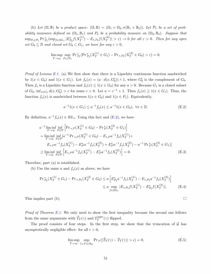
(b) Let (Ω,B) be a product space: (Ω,B) = (Ω1 × Ω2, σ(B1 × B2)). Let P1 be a set of prob-

ability measures defined on (Ω1,B1) and P2 be a probability measure on (Ω2,B2). Suppose that

supP1∈P1Pr ∗P1

(supf∈BL1|E∗P2

f(X(1)T ) − E∗,P2f(X

(2)T )| > ε) → 0 for all ε > 0. Then for any open

set G0 ⊆ D and closed set G0 ⊂ G1, we have for any ε > 0,

lim supT→∞

supP1∈P1

Pr ∗P1(Pr ∗P2

(X(1)T ∈ G1)− Pr ∗,P2(X

(2)T ∈ G0) > ε) = 0.

Proof of Lemma E.1. (a) We first show that there is a Lipschitz continuous function sandwiched

by 1(x ∈ G0) and 1(x ∈ G1). Let fa(x) = (a · d(x,Gc0)) ∧ 1, where Gc0 is the complement of G0.

Then fa is a Lipschitz function and fa(x) ≤ 1(x ∈ G0) for any a > 0. Because G1 is a closed subset

of G0, infx∈G1 d(x,Gc0) > c for some c > 0. Let a = c−1 + 1. Then fa(x) ≥ 1(x ∈ G1). Thus, the

function fa(x) is sandwiched between 1(x ∈ G0) and 1(x ∈ F1). Equivalently,

a−11(x ∈ G1) ≤ a−1fa(x) ≤ a−11(x ∈ G0), ∀x ∈ D. (E.2)

By definition, a−1fa(x) ∈ BL1. Using this fact and (E.2), we have

a−1 lim infT→∞

infP∈P

[Pr ∗,P (X

(1)T ∈ G0)− Pr ∗P (X

(2)T ∈ G1)

]= lim inf

T→∞infP∈P

[a−1 Pr ∗,P (X(1)T ∈ G0)− E∗,Pa−1fa(X

(1)T )+

E∗,Pa−1fa(X

(1)T )− E∗Pa−1fa(X

(2)T ) + E∗Pa

−1fa(X(2)T )− a−1 Pr ∗P (X

(2)T ∈ G1)]

≥ lim infT→∞

infP∈P

[E∗,Pa

−1fa(X(1)T )− E∗Pa−1fa(X

(2)T )]

= 0. (E.3)

Therefore, part (a) is established.

(b) Use the same a and fa(x) as above, we have

Pr ∗P2(X

(1)T ∈ G1)− Pr ∗,P2(X

(2)T ∈ G0) ≤ a

[E∗P2

a−1fa(X(1)T )− E∗,P2a

−1fa(X(2)T )]

≤ a supf∈BL1

|E∗,P2f(X(1)T )− E∗P2

f(X(2)T )|. (E.4)

This implies part (b).

Proof of Theorem E.1. We only need to show the first inequality because the second one follows

from the same arguments with TT (γ) and T apprT (γ) flipped.

The proof consists of four steps. In the first step, we show that the truncation of G has

asymptotically negligible effect: for all ε > 0,

lim supT→∞

sup(γ,F )∈H0

Pr F (|TT (γ)− TT (γ)| > ε) = 0, (E.5)

51

where TT (γ) is the same as TT (γ) except that the integral is over G instead of GT .

In the second step, we define a bounded version of TT (γ): TT (γ;B1, B2) and a bounded version

of T apprT (γ): T apprT (γ;B1, B2) and show that for any B1, B2 > 0 and any real sequence xT ,

lim infT→∞

inf(γ,F )∈H0

[Pr F (TT (γ;B1, B2) ≤ xT + η)− Pr(T apprT (γ;B1, B2) ≤ xT )

]≥ 0. (E.6)

In the third step, we show that TT (γ;B1, B2) is asymptotically close in distribution to TT (γ)

for large enough B1, B2: for any ε > 0, there exists B1,ε and B2,ε such that

lim supT→∞

sup(γ,F )∈H0

Pr F (TT (γ;B1,ε, B2,ε) 6= TT (γ)) < ε. (E.7)

In the fourth step, we show that T apprT (γ;B1, B2) is asymptotically close in distribution to T apprT (γ)

for large enough B1, B2: for any ε > 0, there exists B1,ε and B2,ε such that

lim supT→∞

sup(γ,F )∈H0

Pr F (T apprT (γ;B1,ε, B2,ε) 6= T apprT (γ)) < ε. (E.8)

The four steps combined proves the Theorem. Now we give detailed arguments of the four steps.

STEP 1. First we show a property of the function S that is useful throughout all steps: for

any (m1,Σ1) and (m2,Σ2) ∈ Rk ×Ψξ,

|S(m1,Σ1)− S(m2,Σ2)| ≤ C2 × (S(m2,Σ2) + 1)(∆ +√

∆2 + 8∆)/2, (E.9)

for the ∆ and C in Assumption D.6(b). Let ∆S := |S(m1,Σ1) − S(m2,Σ2)|. Assumption D.6(b)

implies that

∆2S ≤ C2 × (S(m1,Σ1) + S(m2,Σ2))(S(m2,Σ2) + 1)∆

≤ C2 × (∆S + 2S(m2,Σ2))(S(m2,Σ2) + 1)∆. (E.10)

Solve the quadratic inequality for ∆S , we have

∆S ≤C2

2

[(S(m2,Σ2) + 1)∆ +

√(S(m2,Σ2) + 1)2∆2 + 8S(m2,Σ2)(S(m2,Σ2) + 1)∆

]≤ C2

2(S(m2,Σ2) + 1)(∆ +

√∆2 + 8∆) (E.11)

This shows (E.9).

52

Now observe that

0 ≤ TT (γ)− TT (γ)

≤ supθ∈Γ−1(γ)

∫G/GT

S(√T ρT (θ, g), Σι

T (θ, g))dµ(g)

≤ supθ∈Γ−1(γ)

∫G/GT

S(√TρF (θ, g),Σι

F (θ, g))dµ(g)+

supθ∈Γ−1(γ)

∫G/GT

|S(√TρF (θ, g),Σι

F (θ, g))− S(√T ρT (θ, g), Σι

T (θ, g))|dµ(g)

= o(1) + supθ∈Γ−1(γ)

∫G/GT

|S(√TρF (θ, g),Σι

F (θ, g))− S(√T ρT (θ, g), Σι

T (θ, g))|dµ(g)

≤ o(1) + supθ∈Γ−1(γ)

∫G/GT

C2 ×(S(√TρF (θ, g),Σι

F (θ, g)) + 1)dµ(g)×

supθ∈Γ−1(γ),g∈G/GT

c(||νT (θ, g)||2 + ||vech(Σι

F (θ, g)− ΣιT (θ, g))||

)= o(1) + o(1)× c(Op(1))

= op(1), (E.12)

where c(x) = x+√x2 + 8x/2, the third inequality holds by the triangle inequality, the first equality

holds by Assumption D.5(b), the fourth inequality holds by (E.9) and the second equality holds by

Assumptions D.5(a)-(b) and D.2(c)-(d). The o(1), op(1) and Op(1) are uniform over (γ, F ) ∈ H.

Thus, (E.5) is shown.

STEP 2. We define the bounded versions of TT (γ) as

TT (γ;B1, B2) = minθ∈Θ0,F (γ)

minλ∈Λ

B2T (θ,γ)∫

GS(νB1

T (θ + λ/√T , g) +GF (θT , g)λ+

√TρF (θ, g), Σι

T (θ + λ/√T , g))dµ(g) (E.13)

where ΛB2T (θ, γ) = λ ∈ ΛT (θ, γ) : TQF (θ + λ/

√T ) ≤ B2, the process νB1

T (·, ·) = max−B1,

minB1, νT (·, ·) and θT is a value lying on the line segment joining θ and θ + λ/√T satisfying

the mean value expansion:

ρF (θ + λ/√T , g) = ρF (θ, g) +GF (θT , g)λ/

√T . (E.14)

Define the bounded version of T apprT (γ) as

T apprT (γ;B1, B2) = (E.15)

minθ∈Θ0,F (γ)

minλ∈Λ

B2T (θ,γ)

∫GS(νB1

F (θ, g) +GF (θ, g)λ+√TρF (θ, g),Σι

F (θ, g))dµ(g),

53

where νB1F (·, ·) = max−B1,minB1, νF (·, ·).

First we show a useful result: there exists some constant C > 0 such that for all (γ, F ) ∈ H0

and λ ∈ ΛB2T (θ, γ) and for the δ2 in Assumption D.3(b), we have

||λ|| ≤ C × T (δ2−2)/(2δ2). (E.16)

This is shown by observing, for all (γ, F ) ∈ H0 and λ ∈ ΛB2T (θ, γ),

B2 >TQF (θ + λ/√T )

≥C · ((T × d(θ + λ/√T ,Θ0,F (γ))δ2) ∧ (c× T )). (E.17)

The second inequality holds by Assumption (D.3)(b). Because c× T is eventually greater than B2

as T →∞, we have for large enough T ,

B2 ≥ C × T × (||λ||/√T )δ2 . (E.18)

This implies (E.16).

Equation (E.16) implies two results:

(1) sup(γ,F )∈H0

supθ∈Θ0,F (γ)

supλ∈Λ

B2T (θ,γ)

‖λ‖/√T ≤ O(T−1/δ2) = o(1)

(2) sup(γ,F )∈H0

supθ∈Θ0,F (γ)

supλ∈Λ

B2T (θ,γ)

supg∈G‖GF (θ +O(‖λ‖)/

√T , g)λ−GF (θ, g)λ‖

≤ O(1)× ‖λ‖δ1+1T−δ1/2 ≤ O(T (δ2−2(δ1+1))/(2δ2)) = o(1). (E.19)

The first result holds immediately given (E.16) and the second result holds by Assumption D.2(e).

Define an intermediate statistic

TmedT (γ;B1, B2) = minθ∈Θ0,F (γ)

minλ∈Λ

B2T (θ,γ)∫

GS(νB1

T (θ, g) +GF (θ, g)λ+√TρF (θ, g),Σι

F (θ, g))dµ(g). (E.20)

Then TmedT (γ;B1, B2) and T apprT (γ;B1, B2) are respectively the following functional evaluated at

νF (·, ·) and νT (·, ·):

h(ν) = minθ∈Θ0,F (γ)

minλ∈Λ

B2T (θ,γ)

∫GS(νB1(θ, ·) +GF (θ, ·)λ+

√TρF (θ, ·),Σι

F (θ, ·))dµ. (E.21)

The functional h(ν) is uniformly bounded for all large enough T because for any fixed θ ∈ Θ0,F (γ)

54

and λ ∈ ΛB2T (θ, γ),

h(ν) ≤ 2

∫GS(GF (θ, ·)λ+

√TρF (θ, ·),Σι

F (θ, ·))dµ+ 2

∫GS(νB1(θ, ·),Σι

F (θ, ·))dµ

≤ 2 supΣ∈Ψ

S(−B11k,Σ) + 2

∫GS(GF (θ, ·)λ+

√TρF (θ, ·),Σι

F (θ, ·))dµ

≤ 2 supΣ∈Ψ

S(−B11k,Σ) + 2T ×QF (θ + λ/√T )+

C2 × (T ×QF (θ + λ/√T ) + 1) sup

g∈G(∆T (g) +

√∆T (g)2 + 8∆T (g))

≤ 2 supΣ∈Ψ

S(−B11k,Σ) + 2B2 + C2(B2 + 1)× o(1), (E.22)

where ∆T (g) := ‖GF (θ, g)λ +√TρF (θ, g) −

√TρF (θT , g)‖2 + ‖vech(Σι

F (θ, g) − ΣιF (θT , g))‖ and

θT = θ + λ/√T . The first inequality holds by Assumptions D.6(e)-(f), the second inequality holds

by Assumptions D.2(f) and Assumptions D.6(c), the third inequality holds by (E.9) and the last

inequality holds by (E.19).

The functional h(ν) is Lipschitz continuous for all large enough T with respect to the uniform

metric because

|h(ν1)− h(ν2)| ≤ 2C supθ∈Θ0,F (γ)

supλ∈Λ

B2T (θ,γ)

supg∈G‖ν1(θ, g)− ν2(θ, g)‖ · (1 + h(ν1) + 2h(ν2))

≤ C supθ∈Γ−1(γ),g∈G

‖ν1(θ, g)− ν2(θ, g)‖, (E.23)

where C is any constant such that C > 2C× (6 supΣ∈Ψ S(−B11k,Σ) + 6B2 + 1), the first inequality

holds by Assumption D.6(b) and the second holds by (E.22).

Therefore, for any f ∈ BL1 and any real sequence xT , the composite function f (C−1h(·) +

xT ) ∈ BL1. By AssumptionD.2(c), we have

lim supT→∞

sup(γ,F )∈H0

supf∈BL1

|EF f(TmedT (γ;B1, B2) + xT )− Ef(T apprT (γ;B1, B2) + xT )| = 0. (E.24)

This combined with Lemma E.1(a) (with G0 = (−∞, η) and G1 = (−∞, 0]) gives

lim infT→∞

inf(γ,F )∈H0

[Pr F (TmedT (γ;B1, B2) ≤ xT + η)− Pr(T apprT (γ;B1, B2) ≤ xT )

]≥ 0. (E.25)

55

Now it is left to show that TmedT (γ;B1, B2) and TT (γ;B1, B2) are close. First, we have

|TT (γ;B1, B2)− TmedT (γ;B1, B2)|

≤ supθ∈Θ0,F (γ),λ∈Λ

B2T (θ,γ)

∫G

∣∣∣S(νB1T (θ + λ/

√T , g) +GF (θT , g)λ+

√TρF (θ, g), Σι

T (θ + λ/√T , g))

−S(νB1T (θ, g) +GF (θ, g)λ+

√TρF (θ, g),Σι

F (θ, g))∣∣∣ dµ(g)

≤C2 × supθ∈Θ0,F (γ),λ∈Λ

B2T (θ,γ)

maxg∈G

c(∆T (θ, λ, g))×∫G(1 +MT (θ, λ, g))dµ(g), (E.26)

where c(x) = (x+√x2 + 8x)/2, C is the constant in (E.9),

∆T (θ, λ, g) =‖νB1T (θ + λ/

√T , g)− νB1

T (θ, g) +GF (θT , g)λ−GF (θ, g)λ‖2+

‖vech(ΣT (θ + λ/√T , g)− ΣF (θ, g))‖ and

MT (θ, λ, g) =S(νB1T (θ, g) +GF (θ, g)λ+

√TρF (θ, g),Σι

F (θ, g)). (E.27)

Below we show that for any ε > 0, and some universal constant C > 0,

sup(γ,F )∈H0

Pr F

supθ∈Θ0,F (γ),λ∈Λ

B2T (θ,γ),g∈G

∆T (θ, λ, g) > ε

→ 0 and (E.28)

supT

sup(γ,F )∈H0

supθ∈Θ0,F (γ),λ∈Λ

B2T (θ,γ)

∫GMT (θ, λ, g)dµ(g) < C. (E.29)

Once (E.28) and (E.29) are shown, it is immediate that for any ε > 0,

sup(γ,F )∈H0

Pr F

(|TT (γ;B1, B2)− TmedT (γ;B1, B2)| > ε

)→ 0. (E.30)

This combined with (E.25) shows (E.6).

Now we show (E.28) and (E.29). The convergence result (E.28) is implied by the following

results: for any ε > 0,

sup(γ,F )∈H0

Pr F

supθ∈Θ0,F (γ),λ∈Λ

B2T (θ,γ),g∈G

||νB1T (θ + λ/

√T , g)− νB1

T (θ, g)|| > ε

→ 0

sup(γ,F )∈H0

supθ∈Θ0,F (γ),λ∈Λ

B2T (θ,γ),g∈G

||GF (θT , g)λ−GF (θ, g)λ|| → 0 and

sup(γ,F )∈H0

Pr F

supθ∈Θ0,F (γ),λ∈Λ

B2T (θ,γ),g∈G

||vech(ΣT (θ + λ/√T , g)− ΣF (θ, g))|| > ε

→ 0. (E.31)

The first result in the above display holds by the first result in equation (E.19) and the uniform

stochastic equicontinuity of the empirical process νT (·, g) : Γ−1(γ) → Rdm with respect to the

56

Euclidean metric. The uniform equicontinuity is implied by Assumptions D.2(b), (c) and (f) by

Theorem 2.8.2 of van der Vaart and Wellner (1996). The second result in the above display holds

by the second result in (E.19). The third result in (E.31) holds by Assumption D.2(d) and (f).

Result (E.29) holds because for any θ ∈ Θ0,F (γ) and λ ∈ ΛB2T (θ, γ),∫

GMT (θ, λ, g)dµ(g)

≤2

∫GS(νB1

T θ, g),ΣιF (θ, g))dµ(g) + 2

∫GS(GF (θ, g)λ+

√TρF (θ, g),Σι

F (θ, g))dµ(g)

≤ supΣ∈Ψ

S(−B11k,Σ) + 2

∫GS(GF (θ, g)λ+

√TρF (θ, g),Σι

F (θ, g))dµ(g)

≤ supΣ∈Ψ

S(−B11k,Σ) + 2B2 + C2(B2 + 1)× o(1), (E.32)

where the first inequality holds by Assumptions D.6(f), the second inequality holds by Assumption

D.6(c) and the last inequality holds by the second and third inequality in (E.22) and the o(1) is

uniform over (θ, λ).

STEP 3. In order to show (E.7), first extend the definition of TT (γ;B1, B2) from Step 1 to

allow B1 and B2 to take the value ∞ and observe that TT (γ;∞,∞) = TT (γ).

Assumptions D.2 (c) and Lemma E.1 imply that for any ε > 0, there exists B1,ε large enough

such that

lim supT→∞

sup(γ,F )∈H0

Pr F

(sup

θ∈Θ,g∈G‖νT (θ, g)‖ > B1,ε

)< ε. (E.33)

Therefore we have for all B2,

lim supT→∞

sup(γ,F )∈H0

Pr F(TT (γ,∞, B2) 6= TT (γ;B1,ε, B2)

)< ε. (E.34)

To show that T T (γ) and TT (γ;∞, B2) are close for B2 large enough, first observe that:

T T (γ) ≤ supθ∈Θ0,F (γ)

∫GS(νT (θ, g) +

√TρF (θ, g), Σι

T (θ, g))dµ(g)

≤ supθ∈Θ0,F (γ)

∫GS(νT (θ, g), Σι

T (θ, g))dµ(g)

= Op(1) (E.35)

where the first inequality holds because 0 ∈ ΛT (θ, γ), the second inequality holds because ρF (θ, g) ≥0 for θ ∈ Θ0,F (γ) and by Assumption D.6(c), the equality holds by Assumption D.6(a)-(c) and

Assumptions D.2 (c), (d) and (f). The Op(1) is uniform over (γ, F ) ∈ H0.

For any T , γ, B2, if T T (γ) 6= TT (γ;∞, B2), then there must be a θ∗ ∈ Γ−1(γ) such that

57

T ×QF (θ∗) > B2 and∫GS(νT (θ∗, g) +

√TρF (θ∗, g), Σι

T (θ∗, g))dµ(g) < Op(1). (E.36)

But ∫GS(νT (θ∗, g) +

√TρF (θ∗, g), Σι

T (θ∗, g))dµ(g)

≥2−1

∫GS(√TρF (θ∗, g), Σι

T (θ∗, g))dµ(g)−∫GS(−νT (θ∗, g), Σι

T (θ∗, g))dµ(g)

≥2−1

∫GS(√TρF (θ∗, g), Σι

T (θ∗, g))dµ(g)−Op(1)

≥2−1

[TQF (θ∗)−

∫G|S(√TρF (θ∗, ·), Σι

T (θ∗, ·))− S(√TρF (θ∗, ·),Σι

F (θ∗, ·))|dµ]−Op(1)

≥2−1

[TQF (θ∗)− C2 sup

g∈Gc(||vech(Σι

T (θ∗, g)− ΣιF (θ∗, g))||)× (1 + TQF (θ∗))

]−Op(1)

=B2/2− o(1)− op(1)× C2 ×B2/4−Op(1), (E.37)

where c(x) = (x +√x2 + 8x)/2 and C is the constant in (E.9). The first inequality holds by

Assumptions D.6(e)-(f), the second inequality holds by Assumption D.6(c) and Assumptions D.2(c)-

(d) and (f), the third inequality holds by the triangle inequality, the fourth inequality holds by (E.9)

and the equality holds by Assumption D.2(d). The terms o(1), op(1) and Op(1) terms are uniform

over θ∗ ∈ Γ−1(γ) and (γ, F ) ∈ H0.

Then

sup(γ,F )∈H0

Pr F

(T T (γ) 6= TT (γ;∞, B2)

)≤ sup

(γ,F )∈H0

Pr F(2−1(1− op(1))×B2 − o(1)−Op(1) ≤ Op(1)

)= sup

(γ,F )∈H0

Pr F (Op(1) ≥ B2) , (E.38)

where the first inequality holds by (E.36) and (E.37). Then for any ε, there exists B2,ε such that

limT→∞

sup(γ,F )∈H0

Pr F (TT (γ) 6= TT (γ;∞, B2,ε)) < ε. (E.39)

Combining this with (E.34), we have (E.7).

STEP 4. In order to show (E.8), first extend the definition of T apprT (γ;B1, B2) from Step 1 to

allow B1 and B2 to take the value ∞ and observe that T apprT (γ;∞,∞) = T apprT (γ).

By the same arguments as those for (E.34), for any ε and B2, there exists B1,ε large enough so

58

that

lim supn→∞

sup(γ,F )∈H0

Pr F(T apprT (γ;∞, B2) 6= T apprT (γ;B1,ε, B2)

)< ε. (E.40)

Also by the same reasons as those for (E.35), we have

T apprT (γ) ≤ supθ∈Θ0,F (γ)

∫GS(νF (θ, g),Σι

F (θ, g))dµ(g), (E.41)

where the right hand side is a real-valued random variable.

For any T and B2, if T apprT (γ) 6= T apprT (γ;∞, B2,ε), then there must be a θ∗ ∈ Θ0,F (γ), a

λ∗∗ ∈ λ ∈ ΛT (θ∗, γ) : T ×QF (θ∗ + λ/√T ) > B2 such that

I(λ∗∗) < supθ∈Θ0,F (γ)

∫GS(νF (θ, g),Σι

F (θ, g))dµ(g), (E.42)

where I(λ) =∫G S(νF (θ∗, g)+GF (θ∗, g)λ+

√TρF (θ∗, g),Σι

F (θ∗, g))dµ(g). Next we show that if λ∗∗

exists, then there must exists a λ∗ such that

λ∗ ∈ λ ∈ ΛT (θ∗, γ) : T ×QF (θ∗ + λ/√T ) ∈ (B2, 2B2] and

I(λ∗) < supθ∈Θ0,F (γ)

∫GS(νF (θ, g),Σι

F (θ, g))dµ(g). (E.43)

If T ×QF (θ∗+λ∗∗/√T ) ∈ (B2, 2B2], then we are done. If T ×QF (θ∗+λ∗∗/

√T ) > 2B2, there must

be a a∗ ∈ (0, 1) such that T ×QF (θ∗+ a∗λ∗∗/√T ) ∈ (B2, 2B2] because TQF (θ∗+ 0×λ∗∗/

√T ) = 0

and TQF (θ∗ + aλ∗∗/√T ) is continuous in a (by Assumptions D.2(e) and D.6(a)). By Assump-

tion D.6(f), I(λ) is convex. Thus I(a∗λ∗∗) ≤ a∗I(λ∗∗) + (1 − a∗)I(0). For the same argu-

ments as those for (E.35), I(0) ≤ supθ∈Θ0,F (γ)

∫G S(νF (θ, g),Σι

F (θ, g))dµ(g). Thus, I(a∗λ∗∗) <

supθ∈Θ0,F (γ)

∫G S(νF (θ, g),Σι

F (θ, g))dµ(g). Assumption (D.1)(c) and the definition of ΛT (θ, γ) guar-

antee that a∗λ∗∗ ∈ ΛT (θ∗, γ). Therefore, λ∗ = a∗λ∗∗ satisfies (E.43).

Similar to (E.19) we have

(1) ||λ∗||/√T ≤ B2 × 2C × T−1/δ2 = B2 × o(1)

(2) supg∈G||GF (θ∗ +O(||λ∗||)/

√T , g)λ∗ −GF (θ∗, g)λ∗||

≤ O(1)×B(δ1+1)/δ22 ||λ||δ1+1T−δ1/2 = B

(δ1+1)/δ22 o(1), (E.44)

59

where the o(1) terms do not depend on B2. Then,

I(λ∗) ≥ 2−1

∫GS(GF (θ∗, g)λ∗ +

√TρF (θ∗, g),Σι

F (θ∗, g))dµ(g)−∫GS(−νF (θ∗, g),Σι

F (θ∗, g))dµ(g)

≥ TQF (θ∗ + λ∗/√T )/2− C2 × (TQF (θ∗ + λ∗/

√T ) + 1)× c(∆T )/2 +Op(1)

= TQF (θ∗ + λ∗/√T )/2− C2 × (2B2 + 1)× c(∆T )/4 +Op(1), (E.45)

where the Op(1) term is uniform over (γ, F ) ∈ H0, c(x) = (x+√x2 + 8x)/2 and

∆T := ‖GF (θ∗, g)λ∗ +√TρF (θ∗, g)−

√TρF (θ∗ + λ∗/

√T , g)‖2

+ ‖vech(ΣιF (θ∗ + λ∗/

√T , g)− Σι

F (θ∗, g))‖. (E.46)

The first inequality in (E.45) holds by Assumptions D.6(e)-(f), the second inequality holds by

(E.9) and the equality holds by (E.43). By (E.44) and Assumption D.2(f), for any fixed B2,

limT→∞∆T = 0. Therefore, for each fixed B2,

I(λ∗) ≥ TQF (θ∗ + λ∗/√T )/2−Op(1) ≥ B2/2−Op(1). (E.47)

Thus

sup(γ,F )∈H0

Pr(T apprT (γ) 6= T apprT (γ;∞, B2))

≤ sup(γ,F )∈H0

Pr

(sup

θ∈Θ0,F (γ)

∫GS(νF (θ, g),Σι

F (θ, g))dµ(g) ≥ B2/2−Op(1)

)= sup

(γ,F )∈H0

Pr(Op(1) ≥ B2). (E.48)

For any ε > 0, there exists B2,ε large enough so that limT→∞ sup(γ,F )∈H0Pr(Op(1) ≥ B2) < ε.

Thus,

limT→∞

sup(γ,F )∈H0

Pr(T apprT (γ) 6= T apprT (γ;∞, B2,ε) < ε. (E.49)

Combining this with (E.40), we have (E.8).

E.2 Proof of Theorem D.1

The following lemma is used in the proof of Theorem D.1. It shows the convergence of the bootstrap

empirical process ν∗T (θ, g). Let WT,t be the number of times that the tth observation appearing in

a bootstrap sample. Then (WT,1, ...,WT,T ) is a random draw from a multinomial distribution with

60

parameters T and (T−1, ..., T−1), and ν∗T (θ, g) can be written as

ν∗T (θ, g) = T−1/2T∑t=1

(WT,t − 1)ρ(wt, θ, g). (E.50)

In the lemma, the subscripts F and W for E and Pr signify the fact that the expectation and the

probabilities are taken with respect to the randomness in the data and the randomness in WT,trespectively.

Lemma E.2. Suppose that Assumption D.2 holds. Then for any ε > 0,

(a)lim supT→∞ sup(γ,F )∈H Pr ∗F (supf∈BL1|EW f(ν∗T (·, ·))− Ef(νF (·, ·))| > ε) = 0,

(b) there exists Bε large enough such that

lim supT→∞

sup(γ,F )∈H

Pr ∗F

(PrW

(sup

θ∈Γ−1(γ),g∈G||ν∗T (θ, g)|| > Bε

)> ε

)= 0, and

(c) there exists δε small enough such that

lim supT→∞

sup(γ,F )∈H

Pr ∗F

(PrW

(supg∈G

sup||θ(1)−θ(2)||≤δε

||ν∗T (θ(1), g)− ν∗T (θ(2), g)|| > ε

)> ε

)= 0.

Proof of Lemma E.2. (a) Part (a) is proved using a combination of the arguments in Theorem 2.9.6

and Theorem 3.6.1 in van der Vaart and Wellner (1996). Take a Poisson number NT with mean

T and independent from the original sample. Then WNT ,1, ...,WNT ,T are i.i.d. Poisson variables

with mean one. Let the Poissonized version of ν∗T (θ, g) be

νpoiT (θ, g) = T−1/2T∑t=1

(WNT ,t − 1)ρ(wt, θ, g). (E.51)

Theorem 2.9.6 in van der Vaart and Wellner (1996) is a multiplier central limit theorem that shows

that if ρ(wt, θ, g) : (θ, g) ∈ Θ × G is F -Donsker and pre-Gaussian, then νpoiT (θ, g) converges

weakly to νF (θ, g) conditional on the data in outer probability. The arguments of Theorem 2.9.6

remain valid if we strengthen the F -Donsker and pre-Gaussian condition to the uniform Donsker

and pre-Gaussian condition of Assumption D.2(c) and strengthen the conclusion to uniform weak

convergence:

lim supT→∞

sup(γ,F )∈H

Pr ∗F

(supf∈BL1

|EW f(νpoiT (·, ·))− Ef(νF (·, ·))| > ε

)= 0, (E.52)

In particular, the extension to the uniform versions of the first and the third displays in the proof

of Theorem 2.9.6 in van der Vaart and Wellner (1996) is straightforward. To extend the second

display, we only need to replace Lemma 2.9.5 with Proposition A.5.2 – a uniform central limit

theorem for finite dimensional vectors.

61

Theorem 3.6.1 in van der Vaart and Wellner (1996) shows that, under a fixed (γ, F ), the bounded

Lipschitz distance between νpoiT (θ, g) and ν∗T (θ, g) converge to zero conditional on (outer) almost

all realizations of the data. The arguments remain valid if we strengthen the Glivenko-Cantelli

assumption used there to uniform Glivenko-Cantelli (which is implied by Assumption D.2(c)) and

strengthen the conclusion to: for all ε > 0

lim supT→∞

sup(γ,F )∈H

Pr ∗F

(supf∈BL1

|EW f(νpoiT (·, ·))− EW f(ν∗T (·, ·))| > ε

)= 0, (E.53)

Equations (E.52) and (E.53) together imply part (a).

(b) Part (b) is implied by part (a), Lemma E.1(b) and the uniform pre-Gaussianity assumption

(Assumption D.2(c)). When applying Lemma E.1(b), consider X(1)T = ν∗T , X

(2)T = νF , G1 = ν :

supθ,g ‖ν(θ, g)‖ ≥ Bε, and G2 = ν : supθ,g ‖ν(θ, g)‖ > Bε − 1 where Bε satisfies:

sup(γ,F )∈H

Pr

(sup

θ∈Θ,g∈G‖νF (θ, g)‖ > Bε − 1

)< ε/2. (E.54)

Such a Bε exists because ρ(wt, θ, g) : (θ, g) ∈ Θ × G is uniformly pre-Gaussian by Assumption

D.2(c).

(c) Part (c) is implied by part (a), Lemma E.1(b) and the uniform pre-Gaussianity assumption

(Assumption D.2(c)). When applying Lemma E.1(b), consider X(1)T = ν∗T , X

(2)T = νF , G1 =

ν : sup||θ(1)−θ(2)||≤∆ε,g‖ν(θ(1), g) − ν(θ(2), g)‖ ≥ ε, and G0 = ν : sup||θ(1)−θ(2)||≤∆ε,g

‖ν(θ(1), g) −ν(θ(2), g)‖ > ε/2, where ∆ε satisfies:

sup(γ,F )∈H

Pr

(sup

‖θ(2)−θ(2)‖≤∆ε,g

‖νF (θ(1), g)− νF (θ(2), g)‖ > ε/2

)< ε/2. (E.55)

Such a ∆ε exists because ρ(wt, θ, g) : (θ, g) ∈ Θ× G is uniformly pre-Gaussian.

Proof of Theorem D.1. (a) Let qapprbT(γ, p) denotes the p quantile of T apprbT

(γ). Let η2 = η∗/3. Below

we show that,

lim supT→∞

sup(γ,F )∈H0

PrF,sub(csubT (γ, p) ≤ qapprbT

(γ, p) + η2) = 0. (E.56)

where Pr ∗F,sub signifies the fact that there are two sources of randomness in csubT (γ, p) one from the

62

original sampling and the other from the subsampling. Once (E.56) is established, we have,

lim infT→∞

inf(γ,F )∈H0

PrF,sub

(TT (γ) ≤ csubT (γ, p)

)≥ lim inf

T→∞inf

(γ,F )∈H0

PrF

(TT (γ) ≤ qapprbT

(γ, p) + η2

)≥ lim inf

T→∞inf

(γ,F )∈H0

[PrF

(TT (γ) ≤ qapprbT

(γ, p) + η2

)− Pr

(T apprT (γ) ≤ qapprbT

(γ, p))]

+ lim infT→∞

inf(γ,F )∈H0

[Pr(T apprT (γ) ≤ qapprbT

(γ, p))− Pr

(T apprbT

(γ) ≤ qapprbT(γ, p)

)]+ lim inf

T→∞inf

(γ,F )∈H0

Pr(T apprbT

(γ) ≤ qapprbT(γ, p)

)(E.57)

≥ p,

where the first inequality holds by (E.56). The third inequality holds because the first two lim infs

after the second inequality are greater than or equal to zero and the third is greater than or equal

to p. The first lim inf is greater than or equal to zero by Theorem E.1. The second lim inf is greater

than or equal to zero T apprbT(γ) ≥ T apprT (γ) for any γ and T which holds because

√T ≥

√bT and

ΛbT (θ, γ) ⊆ ΛT (θ, γ) for large enough T by Assumptions D.1(c) and D.7(c).

Now it is left to show (E.56). In order to show (E.56), we first show that the c.d.f. of T apprbT(γ)

is close to the following empirical distribution function:

LT,bT (x; γ) = S−1T

ST∑s=1

1(T sT,bT (γ) ≤ x

). (E.58)

Define an intermediate quantity first:

LT,bT (x; γ) = q−1T

qT∑l=1

1(T lT,bT (γ) ≤ x

), (E.59)

where qT = ( TbT ) and (T lT,bT (γ))qTl=1 are the subsample statistics computed using all qT possible

subsamples of size bT of the original sample. Conditional on the original sample, (T sT,bT (γ))STs=1 is

ST i.i.d. draws from LT,bT (·; γ). By the uniform Glivenko-Cantelli theorem, for any ε > 0,

lim supT→∞

sup(γ,F )∈H0

Pr F,sub

(supx∈R

∣∣∣LT,bT (x; γ)− LT,bT (x; γ)∣∣∣ > ε

)= 0 (E.60)

It is implied by a Hoeffding’s inequality (Theorem A on page 201 of Serfling (1980a)) for U-statistics

that for any real sequence xT , and ε > 0,

lim supT→∞

sup(γ,F )∈H0

PrF

(LT,bT (xT ; γ)− PrF

(T lT,bT (γ) ≤ xT

)> ε)

= 0. (E.61)

63

Equations (E.60) and (E.61) imply that, for any real sequence xT and ε > 0,

lim supT→∞

sup(γ,F )∈H0

PrF,sub

(LT,bT (xT ; γ)− PrF

(T lT,bT (γ) ≤ xT

)> ε)

= 0. (E.62)

Apply Theorem E.1 on the subsample statistic T lT,bT (γ), and we have for any ε > 0 and any

real sequence xT ,

lim supT→∞

sup(γ,F )∈H0

[PrF

(T lT,bT (γ) ≤ xT − ε

)− Pr

(T apprbT

(γ) ≤ xT)]

< 0. (E.63)

Equations (E.62) and (E.63) imply that for any real sequence xT ,

sup(γ,F )∈H0

PrF,sub

(LT,bT (xT ; γ) >

(η2 + Pr

(T apprbT

(γ) ≤ xT + η2

)))→ 0. (E.64)

Plug xT = qapprbT(γ, p)− 2η2 into the above equation and we have:

lim supT→∞

sup(γ,F )∈H0

Pr∗F,sub

(LT,bT (qapprbT

(γ, p)− 2η2; γ) > η2 + p)

= 0. (E.65)

However, by the definition of csubT (γ, p), LT,bT (csubT (γ, p)− η∗; γ) ≥ p+ η∗ > η2 + p. Therefore

lim supn→∞

sup(γ,F )∈H0

Pr∗F,sub

(LT,bT (qapprbT

(γ, p)− 2η2; γ) ≥ LT,bT (csubT (γ, p)− η∗; γ))

=0, (E.66)

which implies (E.56).

(b) Let qbtκT (γ, p) be the p quantile of T apprκT (γ) conditional on the original sample. Below we

show that for η2 = η∗/3,

lim supT→∞

sup(γ,F )∈H0

PrF,W (cbtT (γ, p) < qbtκT (γ, p) + η2) = 0. (E.67)

where Pr F,W signifies the fact that there are two sources of randomness in cbtT (γ, p), that from the

original sampling and that from the bootstrap sampling. Once (E.67) is established, we have,

lim infT→∞

inf(γ,F )∈H0

PrF,W

(TT (γ) ≤ cbtT (γ, p)

)≥ lim inf

T→∞inf

(γ,F )∈H0

PrF

(TT (γ) ≤ qbtκT (γ, p) + η2

)≥ lim inf

T→∞inf

(γ,F )∈H0

Pr(T apprT (γ) ≤ qbtκT (γ, p)

)≥ lim inf

T→∞inf

(γ,F )∈H0

Pr(T apprκT

(γ) ≤ qbtκT (γ, p))

= p, (E.68)

where the first inequality holds by (E.67), the second inequality holds by Theorem E.1 and the third

inequality holds because T apprκT (γ) ≥ T apprT (γ) for any γ and T which holds because√T ≥ √κT and

64

ΛκT (θ, γ) ⊆ ΛT (θ, γ) for large enough T by Assumptions D.1(c) and D.7(c).

Now we show (E.67). First, we show that the c.d.f. of T apprκT (γ) is close to the following empirical

distribution:

FST (x, γ) = S−1T

ST∑l=1

1T ∗T,l(γ) ≤ x, (E.69)

where T ∗T,1(γ), ..., T ∗T,ST (γ) are the ST conditionally independent copies of the bootstrap test

statistics. By the uniform Glivenko-Cantelli Theorem, FST (x, γ) is close to conditional c.d.f. of

T ∗T (γ): for any η > 0

lim supT→∞

sup(γ,F )∈H0

Pr F,W

(supx∈R|FSn(x, γ)− PrW (T ∗T (γ) ≤ x)| > η

)= 0. (E.70)

The same arguments as those for Theorem E.1 can be followed to show that T ∗T (γ) is close in

law to T apprκT (γ) in the following sense: for any real sequence xT ,

lim supT→∞

sup(γ,F )∈H0

Pr F([

PrW (T ∗T (γ) ≤ xT − η2)− Pr(T apprκT(γ) ≤ xT )

]≥ η2

)= 0. (E.71)

When following the arguments for Theorem E.1, we simply need to observe the resemblance between

TT (γ) and T ∗T (γ) in the following form:

T ∗T (γ) = minθ∈Θ0,F (γ)

minλ∈ΛκT (θ,γ)∫

GS(ν∗+T (θ + λ/

√T , g) +GF (θT , g)λ+

√κTρF (θ, g), Σn(θ + λ/

√T , g))dµ(g), (E.72)

where

ν∗+T (θ, g) = ν∗T (θ, g) + κ1/2T n−1/2νT (θ, g), (E.73)

and use Lemma E.2 in conjunction with Assumptions D.2(c) and use Lemma E.1(b) in place of

E.1(a).

Equations (E.70) and (E.71) together imply that for any real sequence xT ,

lim supT→∞

sup(γ,F )∈H0

Pr F,W([FST (xT − η2, γ)− Pr(T apprκT

(γ) ≤ xT )]≥ 2η2

)= 0. (E.74)

Plug in xT = qapprκT (γ, p)− η2 and we have

lim supT→∞

sup(γ,F )∈H0

Pr F,W(FST (qapprκT

(γ, p)− 2η2, γ) ≥ p+ 2η2

)= 0. (E.75)

But by definition, FST (cbtT (γ, p)− η∗, γ) ≥ p+ η∗ > p+ 2η2. Therefore,

lim supT→∞

sup(γ,F )∈H0

Pr F,W

(FST (qapprκT

(γ, p)− 2η2, γ) ≥ FST (cbtT (γ, p)− η∗, γ))

= 0, (E.76)

65

which implies (E.67).

References

Andrews, D. W. K., and X. Shi (2013): “Inference Based on Conditional Moment Inequality

Models,” Econometrica, 81.

Bugni, F. A., I. A. Canay, and X. Shi (2016): “Inference for Subvectors and Other Functions

of Partially Identified Parameters in Moment Inequality Models,” Quantitative Economics.

Chernozhukov, V., H. Hong, and E. Tamer (2007): “Estimation and Confidence Regions for

Parameter Sets in Econometric Models,” Econometrica, 75, 1243–1284.

Romano, J., and A. Shaikh (2008): “Inference for Identifiable Parameters in Partially Identified

Econometric Models,” Journal of Statistical Planning and Inference, (Special Issue in Honor of

T. W. Anderson, Jr. on the Occasion of his 90th Birthday), 138, 2786–2807.

Serfling, R. J. (1980a): Approximation Theorems in Mathematical Statistics. John Wiley and

Sons, INC.

van der Vaart, A., and J. Wellner (1996): Weak Convergence and Empirical Processes: with

Applications to Statistics. Springer.

66