Embed Size (px)
Citation preview

1
June 23rd, 2016
ESTIMATING DEMOLITION
IMPACTS IN OHIO Mid-Program Analysis of the
Ohio Housing Finance Agency’s
Neighborhood Initiative Program
www.dynamometrics.com
Abstract This study is a mid-program analysis of the Ohio Housing Finance Agency’s (OHFA) Neighborhood Initiative Program (NIP). Research investigates specific measures of impact associated with home value protection and homeownership preservation as a result of OHFA NIP demolition activity between the beginning of the program in first quarter (Q1) 2014 through the beginning of the second quarter (Q2) of 2016. Given the broad scope of estimating statewide OHFA NIP demolition impacts, a benefits transfer research design was employed that imputes findings from an observational study area (within Cuyahoga County) with rich data resources and high utilization of the OHFA NIP demolition funds into 18 other participating Ohio counties. Considerable limitations exist and are addressed associated with the precision of benefit estimates outside of Cuyahoga County because such estimates rest upon a benefits transfer analysis and not direct observation. The statewide impact from OHFA NIP demolition is estimated at $121.4 million in home value protection with a demolition cost of just over $28.2 million (2,248 demolitions total), or $4.30 in increased home values for every dollar spent. Appendix 10 displays these home value impact results by county submarket. Further, evidence suggests census tracts where demolition activity is taking place have mortgage foreclosure rates that are lower and declining faster than areas without demolition intervention. Visualizations of these trends start at page 34. Both relationships appear to have the strongest impact in the middle value submarket identified in the study.
2
Table of Contents PURPOSE OF THE PROJECT ................................................................................................................... 4
BACKGROUND ....................................................................................................................................... 5
Policy .............................................................................................................................................................................. 5 Distressed Property Literature ........................................................................................................................................ 6
FRAMING THE RESEARCH ..................................................................................................................... 7
Research Questions ........................................................................................................................................................ 8 Research Objectives ....................................................................................................................................................... 8 Research Hypotheses ..................................................................................................................................................... 8 Benefits Transfer Application for Statewide Analysis ...................................................................................................... 8
RESEARCH DESIGN .............................................................................................................................. 10
RESEARCH METHODS: INSTRUMENTS AND MEASURES ................................................................... 13
Two-Stage Multivariate Cluster Analysis ....................................................................................................................... 14 Hedonic Price Function ................................................................................................................................................. 16
Spatial Regimes Hedonic Price Function ....................................................................................................................... 18 Counterfactual Analysis ................................................................................................................................................ 19 Comparative Trends Analysis ........................................................................................................................................ 20 Data .............................................................................................................................................................................. 21
RESULTS ............................................................................................................................................... 23
Two-Stage Multivariate Cluster Analysis ....................................................................................................................... 23 Stage One Multivariate Cluster Analysis Results .......................................................................................................... 24 Stage Two Multivariate Cluster Analysis ....................................................................................................................... 24
Spatial Regimes Hedonic Price Function ....................................................................................................................... 26 Counterfactual Analysis ................................................................................................................................................ 28 Comparative Trends Analysis ........................................................................................................................................ 30
Aggregated Housing Markets in Cuyahoga County Study Area ................................................................................... 31 Lowest Value Housing Submarket Regime in Cuyahoga County Study Area .............................................................. 32 Middle Value Housing Submarket Regime in Cuyahoga County Study Area .............................................................. 33 Highest Value Housing Submarket Regime in Cuyahoga County Study Area ............................................................. 34
STUDY DISCUSSION ............................................................................................................................. 35
Discussion of Benefits Transfer Analysis ........................................................................................................................ 36
KEY INSIGHTS ....................................................................................................................................... 37
REFERENCES ........................................................................................................................................ 38
APPENDIX 1: STAGE 2 K-MEANS CLUSTERING RESULTS FOR STATEWIDE OHFA NIP COUNTY
SUBMARKETS ....................................................................................................................................... 40
Appendix 1.1: Ashtabula County OHFA NIP Submarkets ............................................................................................... 40 Appendix 1.2: Butler County OHFA NIP Submarkets...................................................................................................... 41 Appendix 1.3: Clark County OHFA NIP Submarkets ....................................................................................................... 42 Appendix 1.4: Columbiana County OHFA NIP Submarkets ............................................................................................ 43 Appendix 1.5: Cuyahoga County OHFA NIP Submarkets ................................................................................................ 44 Appendix 1.6: Erie County OHFA NIP Submarkets ......................................................................................................... 45 Appendix 1.7: Fairfield County OHFA NIP Submarkets .................................................................................................. 46 Appendix 1.8: Franklin County OHFA NIP Submarkets ................................................................................................... 47 Appendix 1.9: Hamilton County OHFA NIP Submarkets ................................................................................................. 48 Appendix 1.10: Jefferson County OHFA NIP Submarkets ............................................................................................... 49 Appendix 1.11: Lake County OHFA NIP Submarkets ...................................................................................................... 50 Appendix 1.12: Lucas County OHFA NIP Submarkets .................................................................................................... 51
3
Appendix 1.13: Mahoning County OHFA NIP Submarkets ............................................................................................. 52 Appendix 1.14: Montgomery County OHFA NIP Submarkets......................................................................................... 53 Appendix 1.15: Portage County OHFA NIP Submarkets ................................................................................................. 54 Appendix 1.16: Richland County OHFA NIP Submarkets ................................................................................................ 55 Appendix 1.17: Stark County OHFA NIP Submarkets ..................................................................................................... 56 Appendix 1.18: Summit County OHFA NIP Submarkets ................................................................................................. 57 Appendix 1.19: Trumbull County OHFA NIP Submarkets ............................................................................................... 58
APPENDIX 2: STAGE 1 PRINCIPAL COMPONENTS ANALYSIS RESULTS ............................................. 59
APPENDIX 3: STAGE 1 K-MEANS CLUSTERING RESULTS IN CUYAHOGA COUNTY ........................... 61
APPENDIX 4: STAGE 2 PRINCIPAL COMPONENTS ANALYSIS RESULTS ............................................. 62
APPENDIX 5: FULL LIST AND DEFINITIONS OF HEDONIC PRICE FUNCTION VARIABLES .................. 64
APPENDIX 6: DATA SOURCES AND METADATA ................................................................................. 66
NEOCANDO Raw Data Captured ................................................................................................................................... 66 OHFA NIP Raw Data Captured ....................................................................................................................................... 67 U.S. Census Bureau Raw Data Captured ........................................................................................................................ 67
APPENDIX 7: GLOBAL AND COUNTY LEVEL SUBMARKET SUMMARY STATISTICS ........................... 68
APPENDIX 8: GLOBAL AND THREE-SUBMARKET REGIME HEDONIC MODEL RESULTS.................... 72
APPENDIX 9: THREE-SUBMARKET REGIME HEDONIC MODEL CHOW TEST RESULTS ..................... 73
APPENDIX 10: OHFA NIP BENEFIT-COST RATIO BY COUNTY SUBMARKET ...................................... 74
APPENDIX 11: SENSITIVITY TESTING FOR FINAL SPATIAL REGIMES HEDONIC MODEL IN
CUYAHOGA COUNTY ........................................................................................................................... 75
Appendix 11.1: Sensitivity Test Stage 2 Principal Components Analysis Results in Cuyahoga County ............................ 75 Appendix 11.2: Sensitivity Test Stage 2 K-Means Results in Cuyahoga County .............................................................. 77 Appendix 11.3: Sensitivity Test Three-Submarket Summary Statistics in Cuyahoga County ........................................... 78 Appendix 11.4: Sensitivity Test Spatial Regimes Hedonic Model Results in Cuyahoga County ....................................... 79 Appendix 11.5: Sensitivity Test Spatial Regimes Hedonic Model Chow Test Results in Cuyahoga County ...................... 80
4
Purpose of the Project The Economic Emergency Stabilization Act of 2008 (EESA) authorized the Secretary of the Treasury to
purchase troubled financial assets to protect home values, preserve homeownership, promote economic
growth, and maximize the return on these investments. The program born out of EESA was the Troubled
Asset Relief Program (TARP). TARP eventually included about $38 billion for foreclosure prevention
programs. Initially, $7.7 billion was set aside for the Hardest Hit Fund. The Hardest Hit Fund provided
additional support to 18 states “hardest hit” by the foreclosure crisis. Ohio is one of them. Hardest Hit
Fund is administered by U.S. Department of the Treasury, and has recently been augmented by $2 billion.
By its design Hardest Hit Fund is an innovation program: state governments have proposed what they
think will work best for their communities. Ohio, among others, asked U.S. Treasury for permission to use
some of its allocation to demolish vacant and abandoned houses in quasi-public ownership. U.S. Treasury
allowed blight demolition on the strength of data and analysis conducted by the Griswold Consulting
Group, the predecessor of Dynamo Metrics (Dynamo), in the greater Cleveland marketplace.1 The
Cleveland Study analyzed the effects of blight demolition in greater Cleveland from 2009 to 2013. The
Cleveland Study showed that blight demolition in that period had an overall positive effect on home
values, and was strongly associated with preservation of homeownership (i.e., reduction in mortgage
foreclosure rate).
Building on the Cleveland Study and a subsequent study in Detroit2, this project asks if the Hardest Hit
Fund blight demolition in Ohio administered by the Ohio Housing Finance Agency’s (OHFA) Neighborhood
Initiative Program (NIP) is furthering the intent of Congress in EESA. Specifically, is blight demolition in
Ohio protecting the value of surrounding homes, and; is blight demolition strongly associated with the
preservation of homeownership through the lowering of localized mortgage foreclosure rates. Recent
criticism of the Hardest Hit Fund suggests that the state governments do not know if Hardest Hit Fund
demolitions are effective in furthering Congressional intent. Through this study, the Ohio Housing Finance
Agency has measured to what extent early Hardest Hit Fund expenditures have achieved EESA’s
legislative goals of protecting home values and preserving homeownership.
Further, this study is designed to provide decision support to leaders at OHFA and its local partners who
must choose which structures to demolish in the months to come. Because rich property data was not
available in any county but Cuyahoga, we have adapted existing econometric methods and models to
provide OHFA and its local partners outside Cuyahoga with what we think is the best information
available for decision support. We welcome professional feedback on the methods employed in this
exercise in the emerging discipline of property intervention decision support.
1Griswold, N., Calnin. B., Schramm, M., Anselin, L. and P. Boehnlein. 2014. Estimating the Effect of Demolishing Distressed
Structures in Cleveland, OH, 2009-2013: Impacts on Real Estate Equity and Mortgage-Foreclosure. Publication of the Western
Reserve Land Conservancy: Thriving Communities Institute. See:
http://www.neighborhoodindicators.org/library/catalog/estimating-effect-demolishing-distressed-structures-cleveland-oh-2009-
2013. 2 Dynamo Metrics. 2015. Estimating the Home Equity Impacts from Rapid, Targeted Residential Demolition in Detroit, MI: Application of a Spatially-Dynamic Data System for Decision Support. Collaborative publication of Rock Ventures and the Skillman Foundation. See: http://www.demolitionimpact.org/#thereport.
5
Background
Policy Federal housing policy focuses on building new units. The well-established pathways of federal
participation in housing finance - from the Low Income Housing Tax Credit (LIHTC), to Community
Reinvestment Act (CRA) financing, to the programs of the Federal Housing Administration (FHA) and the
Government Sponsored Entities, among others – focus on putting more Americans in more houses.
America’s population is growing, and the creation of good, and often owner-occupied, housing remains a
universally-supported priority of the federal government.
But in large sections of the United States - primarily the legacy industrial areas of the Midwest, Northeast,
and Southeast – real estate markets are burdened with an oversupply of functionally obsolete housing.
Much was built near factories that closed long ago. Most is approaching one-hundred years-old, or older,
and is located in areas that have seen massive out-migration to other areas in nearby regions or across
the country. And, most importantly, this housing is largely located in low-demand markets. Over the last
generation much of this housing has been neglected and abandoned, and the foreclosure crisis made the
problem more acute.
Meanwhile, federal housing policy in those areas, like in the rest of the country, appears focused on
making more units, and not removal of the existing oversupply of blighted or obsolescent units. The
Neighborhood Stabilization Programs (NSP), for example, only allowed 10% of a community’s grant to be
used for demolition. Getting above this cap required a waiver. Likewise, there is no equivalent to LIHTC to
help communities improve low-income neighborhoods by eliminating the abandoned houses burdening
those communities; the program focuses on creating new units. The CRA structure does not seem to
allow banks to earn CRA credits for assisting communities with blight elimination requirements. And so
on.
In light of this emphasis on building new units, U.S. Treasury’s decision to allow some states to use
Hardest Hit Fund allocations for blight demolition represents something of an innovation in federal policy.
Under NIP and similar programs in other states, local governments are able to demolish vacant and
blighted structures with federal funds. The recent decision of Congress to enhance the Hardest Hit Fund
by $2 billion means blight demolition will occur at a large scale, in Ohio and in other states.3
These large-scale demolition programs can be observed and analyzed to evaluate their effectiveness. To
questions like, “Does demolition of blight make neighborhoods safer and more stable?” and “What is the
benefit-cost ratio (BCR)4 of publicly-financed blight demolition for property tax revenue collections?”,
there has been no way to provide a scientifically rigorous answer. Due to advances in economic modeling
3 See U.S. Treasury Press Release dated April 20, 2016 for details: https://www.treasury.gov/press-center/press-releases/Pages/jl0434.aspx. 4 In previous Griswold and Dynamo Metrics reports (see Griswold (2006), Griswold & Norris (2007), Griswold et al. (2014), and Dynamo Metrics (2015)), the benefit-cost ratio (BCR), which measures total home value preservation amount divided by total demolition cost, has been referred to as “return on investment” or “ROI,” and “cost-benefit ratio” or “CBR.” Moving forward, this ratio will consistently be termed benefits-cost ratio (BCR) as standardly defined: http://web.stanford.edu/group/FRI/indonesia/newregional/lectures/lecture7/lecture7BW.pdf
6
and the introduction of “big data” capabilities to real estate information over the past decade,
policymakers can start to objectively explore the potential benefits of making blight removal a central
tenet of federal housing policy in industrial legacy communities.
Distressed Property Literature The impacts of distressed properties and demolition on nearby housing can be measured using a hedonic
price function5, which estimates the marginal implicit value of structural and neighborhood characteristics
associated with residential housing (Taylor, 2003). In other words, this approach provides a dollar value or
percent impact on home value from a marginal increase (i.e. change by one unit) in housing attributes.
For example, an additional bedroom or bathroom becomes explicitly known with this method, as well as
unobserved “spillover” effects from the environment, such as the marginal impact on home value from
an additional nearby distressed property or other disamenity.
The hedonic price function is the econometric modeling tool of choice to measure spillover effects from
distress in the housing market, and has been leveraged regularly in the literature to better understand
the financial and market impacts of distressed property dynamics. The use of the hedonic price function
for measuring the impacts of distressed property and demolition is contemporary in the literature. The
research methods the Dynamo team has employed in this study are the artifacts of a scholarly process
that has unfolded over the past 40 years. While academia and associated scholarly rigor has worked to
solve the myriad econometric modeling and microeconomic theory issues associated with spatially
dependent urban real-estate markets, extensive real-world observational research has applied these
theoretical models into a dynamic policy space.6
While specific econometric methods vary, the negative spillover effects on real estate markets from
nearby distressed properties has been well established in the literature for over 15 years.7 While the
impacts caused by distressed properties are well documented, little scholarly work simulates the dynamic
financial effect of demolition in distressed housing markets. Griswold (2006), Griswold and Norris (2007),
Griswold et al. (2014) and Dynamo Metrics (2015) focus on these dynamics, using the predictive
capabilities of the hedonic price function to estimate home value impact benefits captured by homes
near demolition activity.
5 See Rosen (1974). 6 See Griswold et al. (2014), pgs. 11-15 for a history of the scholarly process. 7 See Simons, Quercia and Maric, 1998; Immergluck and Smith, 2006; Griswold, 2006; Griswold and Norris, 2007; Schuetz, et al., 2008; Mikelbank, 2008; Leonard and Murdoch, 2009; Harding, et al., 2009; Rogers and Winter, 2009; Lin, Rosenblatt and Yao, 2009; Kobie 2009; Rogers, 2010; Hartley, 2010; Campbell et al., 2011; Groves and Rogers, 2011; Whitaker and Fitzpatrick, 2013; Griswold et al., 2014; Dynamo Metrics, 2015; Immergluck, 2015.
7
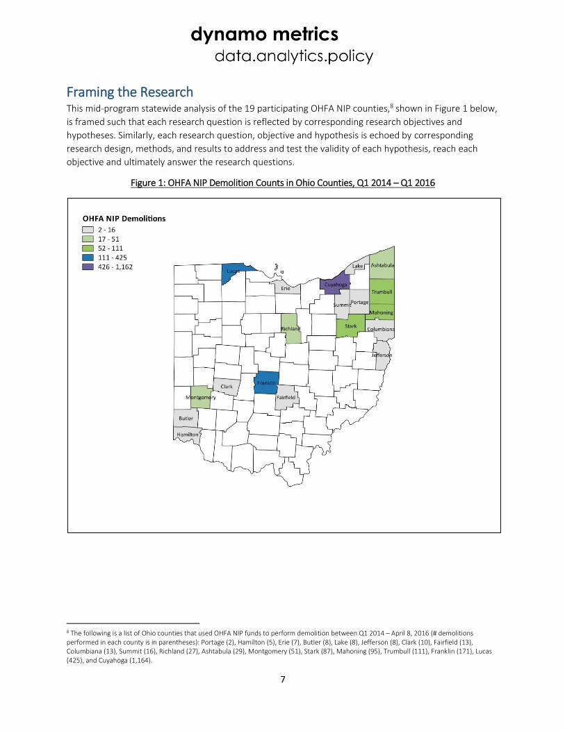
Framing the Research This mid-program statewide analysis of the 19 participating OHFA NIP counties,8 shown in Figure 1 below,
is framed such that each research question is reflected by corresponding research objectives and
hypotheses. Similarly, each research question, objective and hypothesis is echoed by corresponding
research design, methods, and results to address and test the validity of each hypothesis, reach each
objective and ultimately answer the research questions.
Figure 1: OHFA NIP Demolition Counts in Ohio Counties, Q1 2014 – Q1 2016
8 The following is a list of Ohio counties that used OHFA NIP funds to perform demolition between Q1 2014 – April 8, 2016 (# demolitions performed in each county is in parentheses): Portage (2), Hamilton (5), Erie (7), Butler (8), Lake (8), Jefferson (8), Clark (10), Fairfield (13), Columbiana (13), Summit (16), Richland (27), Ashtabula (29), Montgomery (51), Stark (87), Mahoning (95), Trumbull (111), Franklin (171), Lucas (425), and Cuyahoga (1,164).
8
Research Questions This research is driven by an overarching policy question: Is the early Hardest Hit Fund blight demolition
administered across 19 counties in Ohio by OHFA NIP furthering the intent of Congress in EESA? Testing
this policy question with objective scientific methods is driven by two primary research questions:
1. Is blight demolition administered by OHFA NIP in Ohio associated with a stabilization in residential
property values?
2. Is blight demolition administered by OHFA NIP in Ohio associated with a reduction in mortgage
foreclosure rates?
Research Objectives The two primary research questions above are echoed by the primary research objectives of the study:
1. To estimate the impact of OHFA NIP administered HHF demolition programs across Ohio on home
value stabilization;
2. To analyze the strength of the relationship between OHFA NIP administered HHF demolition
programs across Ohio with reductions in localized mortgage foreclosure rates.
Research Hypotheses Research objectives associated with OHFA NIP administered HHF demolition programs are testable with specific analytic hypotheses:
1. If OHFA NIP residential demolition activity occurs in a neighborhood, then home values in the immediate environment will increase relative to areas without demolition;
a. If an additional county land bank owned residential structure9 is within 500 feet of a home, then the home will sell for less, all else equal.
b. If an additional vacant residential lot is within 500 feet of a home, then the home will sell for more than if the vacant residential lot was actually a county land bank-owned residential structure, all else equal.
c. Null hypothesis: The number of county land bank structures and residential vacant lots do not have a measurable impact on home values.
2. If OHFA NIP residential demolition activity occurs in a neighborhood, then mortgage foreclosure rates in the immediate environment will decrease over time.
a. If a neighborhood experiences demolition, then it will experience lower rates of mortgage foreclosure over time, all else equal.
b. Null hypothesis: There is no association between mortgage foreclosure rates and demolition activity.
Benefits Transfer Application for Statewide Analysis This study introduces the framing of a methodological challenge that has not been included in previous
distressed property impact studies conducted by researchers at Dynamo or within the distressed
9 Under Treasury and NIP rules, properties eligible for demolition must be quasi-publicly owned (county land banks in Ohio). This means that every NIP demolished structure was a county land bank-owned house immediately before it was demolished. The study’s comparison is “before” and “after”, which therefore means “county land bank-owned house” and “vacant lot,” respectively. The study assumes non-redevelopment of the subsequent vacant lots during the time-period of the study.
9
property academic field. With 19 counties10 where NIP demolition activity has occurred since the
beginning of the program and a charge of performing a mid-program review that estimates
comprehensive statewide impacts, a benefits transfer11 method was designed so application of findings
from a single sample area could be extrapolated to similar areas throughout Ohio. The clear best practice
would be to perform an original study in each of the 19 counties, but only Cuyahoga County had the
necessary data to perform this research, due to the prior study conducted there and the volume of
demolition activity there (over 50% of OHFA NIP funds had been spent in Cuyahoga County as of April 8,
2016).
The conceptual framework of the benefits transfer approach is well documented in the literature, and speaks to the application of econometric findings in one set of communities to similar areas elsewhere when analysts are faced with time or monetary constraints (see Rosenberger and Loomis, 2003). Use of the benefits transfer requires a strong assumption, however: that Cuyahoga County’s housing market dynamics reasonably approximates the housing dynamics in the other 18 counties. Because that assumption remains untested, we acknowledge this study’s inherent weakness in that regard.
10 19 Ohio counties that used OHFA NIP funds to perform demolition between Q1 2014 – April 8, 2016: Ashtabula, Butler, Clark, Columbiana, Cuyahoga, Erie, Fairfield, Franklin, Hamilton, Jefferson, Lake, Lucas, Mahoning, Montgomery, Portage, Richland, Summit, Stark, and Trumbull. 11 See Chapter 12 (pg. 445) for full explanation of the benefits transfer method: Rosenberger, R.S., and J.B. Loomis. 2003. “Benefits Transfer.” Chapter 12 in (Champ et al. eds.) A Primer for Non-Market Valuation. Kluwer Academic Publishers: Netherlands. pp. 331-393.
10
Research Design The statewide impact element of the research design is the transfer of demolition impact findings from
the estimated hedonic price function in the Cuyahoga County study area (“Observational Study Area”),12
to alike13 Census Tracts in the other 18 counties that received HHF demolition in Ohio (“Benefits Transfer
Study Area”).14 Under a set of restrictive assumptions, this design allows the transfer of findings from the
Observational Study Area to the Benefits Transfer Study Area. While limited, this design attempts to reach
the goal of estimating statewide OHFA NIP demolition impact by transferability of results from one
sample area to other participating areas without an actual empirical study in the 18 remaining areas.
Upon identification of the Observational Study Area and its relative “alikeness” to the Census Tracts in the
18 Benefits Transfer Study Area counties, detailed research in the Observational Study Area could begin.
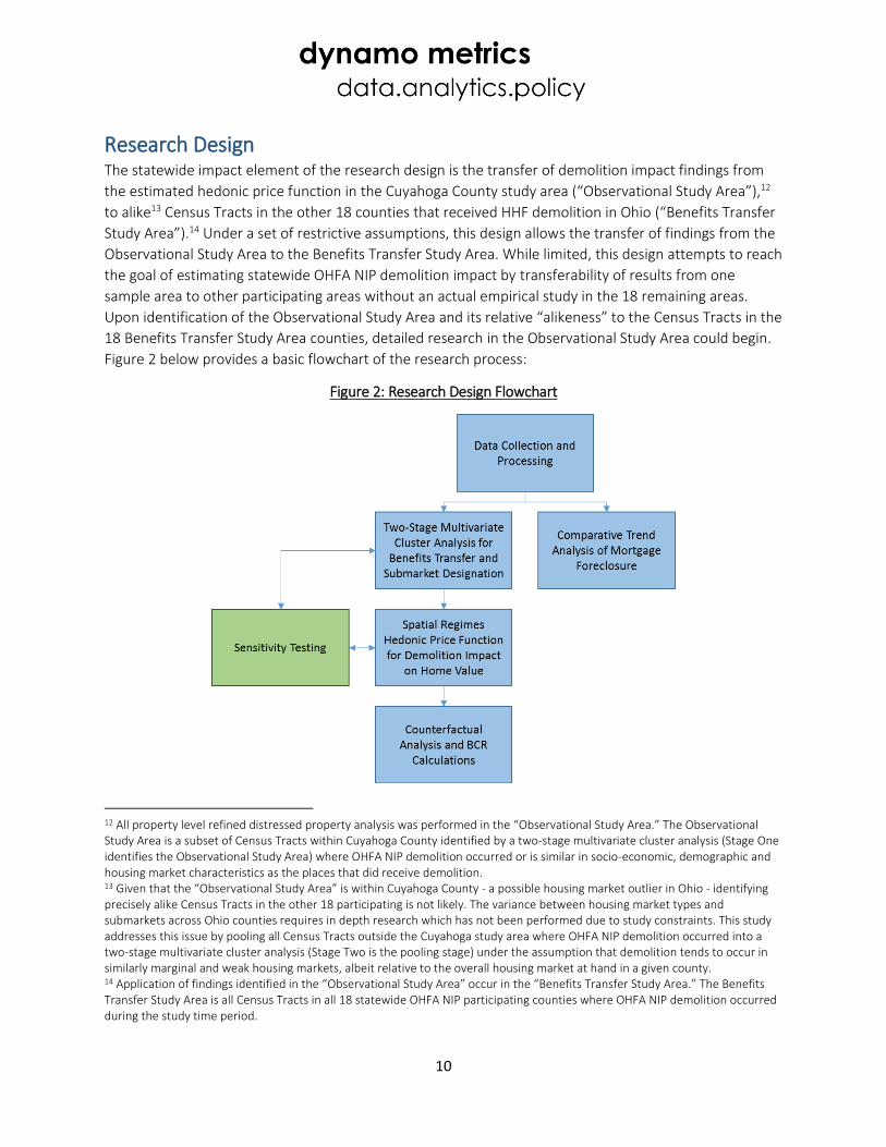
Figure 2 below provides a basic flowchart of the research process:
Figure 2: Research Design Flowchart
12 All property level refined distressed property analysis was performed in the “Observational Study Area.” The Observational Study Area is a subset of Census Tracts within Cuyahoga County identified by a two-stage multivariate cluster analysis (Stage One identifies the Observational Study Area) where OHFA NIP demolition occurred or is similar in socio-economic, demographic and housing market characteristics as the places that did receive demolition. 13 Given that the “Observational Study Area” is within Cuyahoga County - a possible housing market outlier in Ohio - identifying precisely alike Census Tracts in the other 18 participating is not likely. The variance between housing market types and submarkets across Ohio counties requires in depth research which has not been performed due to study constraints. This study addresses this issue by pooling all Census Tracts outside the Cuyahoga study area where OHFA NIP demolition occurred into a two-stage multivariate cluster analysis (Stage Two is the pooling stage) under the assumption that demolition tends to occur in similarly marginal and weak housing markets, albeit relative to the overall housing market at hand in a given county. 14 Application of findings identified in the “Observational Study Area” occur in the “Benefits Transfer Study Area.” The Benefits Transfer Study Area is all Census Tracts in all 18 statewide OHFA NIP participating counties where OHFA NIP demolition occurred during the study time period.
11
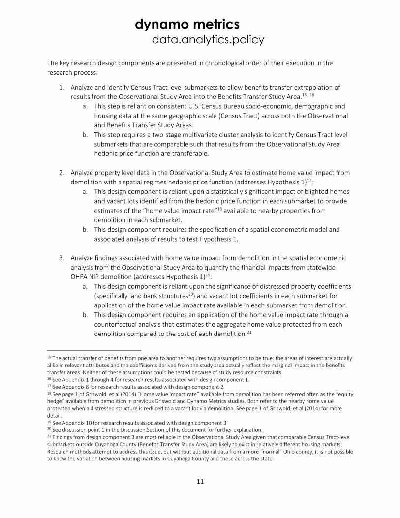
The key research design components are presented in chronological order of their execution in the
research process:
1. Analyze and identify Census Tract level submarkets to allow benefits transfer extrapolation of
results from the Observational Study Area into the Benefits Transfer Study Area.15 , 16
a. This step is reliant on consistent U.S. Census Bureau socio-economic, demographic and
housing data at the same geographic scale (Census Tract) across both the Observational
and Benefits Transfer Study Areas.
b. This step requires a two-stage multivariate cluster analysis to identify Census Tract level
submarkets that are comparable such that results from the Observational Study Area
hedonic price function are transferable.
2. Analyze property level data in the Observational Study Area to estimate home value impact from
demolition with a spatial regimes hedonic price function (addresses Hypothesis 1)17;
a. This design component is reliant upon a statistically significant impact of blighted homes
and vacant lots identified from the hedonic price function in each submarket to provide
estimates of the “home value impact rate”18 available to nearby properties from
demolition in each submarket.
b. This design component requires the specification of a spatial econometric model and
associated analysis of results to test Hypothesis 1.
3. Analyze findings associated with home value impact from demolition in the spatial econometric
analysis from the Observational Study Area to quantify the financial impacts from statewide
OHFA NIP demolition (addresses Hypothesis 1)19:
a. This design component is reliant upon the significance of distressed property coefficients
(specifically land bank structures20) and vacant lot coefficients in each submarket for
application of the home value impact rate available in each submarket from demolition.
b. This design component requires an application of the home value impact rate through a
counterfactual analysis that estimates the aggregate home value protected from each
demolition compared to the cost of each demolition.21
15 The actual transfer of benefits from one area to another requires two assumptions to be true: the areas of interest are actually alike in relevant attributes and the coefficients derived from the study area actually reflect the marginal impact in the benefits transfer areas. Neither of these assumptions could be tested because of study resource constraints. 16 See Appendix 1 through 4 for research results associated with design component 1. 17 See Appendix 8 for research results associated with design component 2. 18 See page 1 of Griswold, et al (2014) ”Home value impact rate” available from demolition has been referred often as the “equity hedge” available from demolition in previous Griswold and Dynamo Metrics studies. Both refer to the nearby home value protected when a distressed structure is reduced to a vacant lot via demolition. See page 1 of Griswold, et al (2014) for more detail. 19 See Appendix 10 for research results associated with design component 3 20 See discussion point 1 in the Discussion Section of this document for further explanation. 21 Findings from design component 3 are most reliable in the Observational Study Area given that comparable Census Tract-level submarkets outside Cuyahoga County (Benefits Transfer Study Area) are likely to exist in relatively different housing markets. Research methods attempt to address this issue, but without additional data from a more “normal” Ohio county, it is not possible to know the variation between housing markets in Cuyahoga County and those across the state.
12
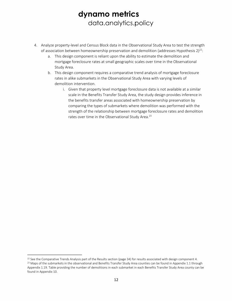
4. Analyze property-level and Census Block data in the Observational Study Area to test the strength
of association between homeownership preservation and demolition (addresses Hypothesis 2)22:
a. This design component is reliant upon the ability to estimate the demolition and
mortgage foreclosure rates at small geographic scales over time in the Observational
Study Area.
b. This design component requires a comparative trend analysis of mortgage foreclosure
rates in alike submarkets in the Observational Study Area with varying levels of
demolition intervention.
i. Given that property level mortgage foreclosure data is not available at a similar
scale in the Benefits Transfer Study Area, the study design provides inference in
the benefits transfer areas associated with homeownership preservation by
comparing the types of submarkets where demolition was performed with the
strength of the relationship between mortgage foreclosure rates and demolition
rates over time in the Observational Study Area.23
22 See the Comparative Trends Analysis part of the Results section (page 34) for results associated with design component 4. 23 Maps of the submarkets in the observational and Benefits Transfer Study Area counties can be found in Appendix 1.1 through Appendix 1.19. Table providing the number of demolitions in each submarket in each Benefits Transfer Study Area county can be found in Appendix 10.
13
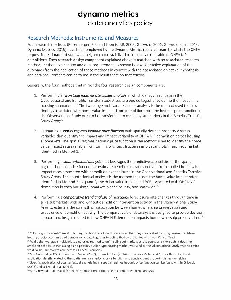
Research Methods: Instruments and Measures Four research methods (Rosenberger, R.S. and Loomis, J.B, 2003; Griswold, 2006; Griswold et al., 2014; Dynamo Metrics, 2015) have been employed by the Dynamo Metrics research team to satisfy the OHFA request for estimates of statewide neighborhood stabilization impacts attributable to OHFA NIP demolitions. Each research design component explained above is matched with an associated research method, method explanation and data requirement, as shown below. A detailed explanation of the outcomes from the application of these methods in concert with their associated objective, hypothesis and data requirements can be found in the results section that follows. Generally, the four methods that mirror the four research design components are:
1. Performing a two-stage multivariate cluster analysis in which Census Tract data in the Observational and Benefits Transfer Study Areas are pooled together to define the most similar housing submarkets.24 The two-stage multivariate cluster analysis is the method used to allow findings associated with home value impacts from demolition from the hedonic price function in the Observational Study Area to be transferable to matching submarkets in the Benefits Transfer Study Area;25
2. Estimating a spatial regimes hedonic price function with spatially defined property distress variables that quantify the impact and impact variability of OHFA NIP demolition across housing submarkets. The spatial regimes hedonic price function is the method used to identify the home value impact rate available from turning blighted structures into vacant lots in each submarket identified in Method 1.;26
3. Performing a counterfactual analysis that leverages the predictive capabilities of the spatial regimes hedonic price function to estimate benefit-cost ratios derived from applied home value impact rates associated with demolition expenditures in the Observational and Benefits Transfer Study Areas. The counterfactual analysis is the method that uses the home value impact rates identified in Method 2 to quantify the dollar value impact and BCR associated with OHFA NIP demolition in each housing submarket in each county, and statewide;27
4. Performing a comparative trend analysis of mortgage foreclosure rate changes through time in alike submarkets with and without demolition intervention activity in the Observational Study Area to estimate the strength of association between homeownership preservation and prevalence of demolition activity. The comparative trends analysis is designed to provide decision support and insight related to how OHFA NIP demolition impacts homeownership preservation.28
24 “Housing submarkets” are akin to neighborhood typology clusters given that they are created by using Census Tract-level housing, socio-economic and demographic data together to define the key attributes of a given Census Tract. 25 While the two-stage multivariate clustering method to define alike submarkets across counties is thorough, it does not ameliorate the issue that a single and possibly outlier type housing market was used as the Observational Study Area to define what “alike” submarkets are across OHFA NIP counties. 26 See Griswold (2006), Griswold and Norris (2007), Griswold et al. (2014) or Dynamo Metrics (2015) for theoretical and application details related to the spatial regimes hedonic price function and spatial-count property distress variables. 27 Specific application of counterfactual analysis from a spatial regimes hedonic price function can be found within Griswold (2006) and Griswold et al. (2014). 28 See Griswold et al. (2014) for specific application of this type of comparative trend analysis.

14
Two-Stage Multivariate Cluster Analysis Given study constraints, it was not possible to implement a full-fledged hedonic analysis for the 19 Ohio
counties with NIP activity. In order to impute results for the 18 remaining counties from the analysis
carried out for the Cuyahoga County Observational Study Area, it is imperative that the Census Tracts
under study are “as similar” as possible.29 To accomplish this, a two-stage multivariate cluster analysis
was carried out. Stage One consisted of an analysis of all the Census Tracts in Cuyahoga County. A
principal components analysis (PCA)30 was carried out using the 23 census variables that were available
for all Census Tracts in the study (both Cuyahoga County and the 18 others).31 Subsequently, the
computed values for the two main components (which explained 50.85% of the total variance) were used
as the basis for a k-means clustering32 exercise. The value of k was varied from 3 to 6 to identify the most
appropriate cluster size.33 34 Close examination of the cluster fit statistics suggested k=4 as the cluster
size. An analysis of the characteristics of the four clusters revealed that all the Census Tracts with NIP
activity were concentrated primarily in two clusters. The Census Tracts in those two clusters35 were then
selected for subsequent analysis in a pooled setting with Census Tracts from the remaining 18 counties
(the other Census Tracts in Cuyahoga county were not included in the subsequent hedonic analysis).
In Stage Two, this exercise was repeated, but now for the selected Observational Study Area Census
Tracts from Cuyahoga County (those tracts in the two identified clusters from the first phase analysis)
29 An observation from outside this study supports use of this study’s benefits transfer analysis, despite the methodological
weakness set forth above and elsewhere in this study. The impact of vacant lots and distressed structures, when statistically
significant within an identified submarket, have been shown to be relatively consistent throughout previous studies as well as the
current one (See Immergluck (2015), Griswold et al. (2014) and Appendix 10). Specifically, the negative impact of an additional
nearby vacant lot tends to decrease home value by 0.5%-1.5% (Griswold et al. (2014) and Appendix 10) and the negative impact
of an additional nearby distressed structure tends to fall between 1.8%-5.2% (Immergluck, 2015), depending on submarket and
distress type (it does tend to be higher in highest value submarkets where demolition does not occur in high frequency). Given
this relative consistency in negative property impacts across studies, transferring benefits estimates of home value impact rates
to other counties where the real Census Tract-level median household incomes are used to quantify home value impacts
provides a reasonable estimation of the impact of demolition in those locations. The benefits transfer analysis further rests upon
a herein untested but common-sense observation that most OHFA NIP demolition activity is occurring in weak-market urban
areas that have, broadly speaking, market dynamics more similar to each other’s than to strong-market areas in each’s own
county (i.e., a real estate market in a depressed inner-city neighborhood in Columbus behaves more like a depressed inner-city
neighborhood housing market in Cleveland than it does to the real estate market in Dublin or Bexley). The summary statistics
from this study do support this assumption given that 75% of sales observations sold for under $65,000 and 50% of sales
observations sold for less than $30,000. 30 Principal components analysis allows a researcher to summarize large correlated sets of variables with smaller numbers of representative variables that collectively explain the majority of variation in the original dataset (G. James, et al., 2013). 31 Identified principal components used for Stage One can be found in Appendix 2. 32 K-means (MacQueen, 1967) is a highly used spatial clustering method, used in our case for similarity grouping of the predicted values of the highest impact PCA outputs for Census Tract submarkets. The method imposes “k” breaks on an “N” dimensional dataset in which mean variance is maximized across “k” breaks and minimized within the “k” breaks. 33 Results from the Stage One k-means analysis can be found in the map in Appendix 3. The two clusters chosen from Stage One where demolition occurred or are like the Census Tracts where demolition occurred are green and grey in Appendix 3. 34 A Stage One multivariate cluster analysis where k=3 was run for sensitivity testing of the final model in Cuyahoga County alone. The sensitivity test was run such that the final model could be run ONLY on the submarket regime in Cuyahoga, as opposed to the pooled Stage Two version, such that a sense of what was “given up” by pooling the 18 county Census Tracts into the final model submarkets is given. Results from the sensitivity analysis can be found in Appendix 11.1 through 11.5. 35 A small number of Census Tract that had demolition occur within them did fall outside of the two primary clusters. These Census Tracts were captured directly and included in the second stage of the cluster analysis.
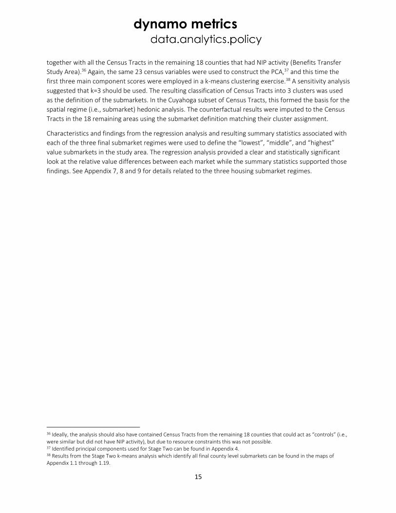
15
together with all the Census Tracts in the remaining 18 counties that had NIP activity (Benefits Transfer
Study Area).36 Again, the same 23 census variables were used to construct the PCA,37 and this time the
first three main component scores were employed in a k-means clustering exercise.38 A sensitivity analysis
suggested that k=3 should be used. The resulting classification of Census Tracts into 3 clusters was used
as the definition of the submarkets. In the Cuyahoga subset of Census Tracts, this formed the basis for the
spatial regime (i.e., submarket) hedonic analysis. The counterfactual results were imputed to the Census
Tracts in the 18 remaining areas using the submarket definition matching their cluster assignment.
Characteristics and findings from the regression analysis and resulting summary statistics associated with
each of the three final submarket regimes were used to define the “lowest”, “middle”, and “highest”
value submarkets in the study area. The regression analysis provided a clear and statistically significant
look at the relative value differences between each market while the summary statistics supported those
findings. See Appendix 7, 8 and 9 for details related to the three housing submarket regimes.
36 Ideally, the analysis should also have contained Census Tracts from the remaining 18 counties that could act as “controls” (i.e., were similar but did not have NIP activity), but due to resource constraints this was not possible. 37 Identified principal components used for Stage Two can be found in Appendix 4. 38 Results from the Stage Two k-means analysis which identify all final county level submarkets can be found in the maps of Appendix 1.1 through 1.19.

16
Hedonic Price Function The hedonic price function was utilized to estimate the impact of OHFA NIP demolition on home values in
this study. Estimating a hedonic price function is an econometric method based on the economic theory
that goods are ultimately valued by way of their utility-bearing attributes (Lancaster, 1966; Rosen, 1974).
Given a competitive market, buyers are assumed to sort themselves by deciding on a “bundle” of
attributes (i.e. a house) that they are willing to purchase, given their income constraints and preferences.
The implicit prices of housing attributes will be decided by the supply of and demand for those particular
housing attributes within the specified area (Deaton, 2002). The intuitive idea is that a house is made of
its physical and structural attributes, as well as all the attributes of its particular environment and
location. According to economic theory, the positive and negative value effects of these attributes are
what make the price of a home higher or lower, respectively.39
If levels of non-market attributes such as disamenities associated with distressed structures and vacant
lots can be measured correctly, a hedonic pricing model can be specified to examine the extent that
variation in the non-market attribute is incorporated in the price of the final product (Deaton 2002).
Multiple studies over the past decade have consistently shown that property distress can be measured
well by using spatially defined variables that aggregate counts of distressed structures and vacant lots in
the immediate environment surrounding a home in the time period it sold.40 A conceptual layout of this
approach is shown in Figure 3, below. Other key hedonic methodological elements critical to this study
that were gleaned from previous similar research include space-time lag variables and submarket regimes
to address spatial error, and standard corrections for heteroscedasticity, among others.41
Figure 3: Conceptual Layout of 500 Foot Buffer to Count Distress Near Home Sales Observations
39 Even in the absence of an efficient market, a hedonic specification is useful as an empirical measure of the relationship between house attributes and the sales price. 40 See Immergluck (2015) 41 See theoretical and methodological sections of Griswold (2006), Griswold et al. (2014) and Dynamo Metrics (2015) for specific detail related to hedonic price function specification.

17
The hedonic price function was specified such that the price of a single-family residential housing unit is
assumed to be a function of the bundle of attributes that characterize the house. The empirical
specification used for the hedonic price function in this study is:
𝑙𝑛(𝑃𝑖) = 𝛽0 + 𝛽1(𝑆𝑇𝑖) + 𝛽2(𝐷𝑖𝑆) + 𝛽2(𝐷𝑖
𝑉𝐿) + 𝛩𝑊𝑖 + 𝛷𝑋𝑖 + 𝛹𝑌𝑖 + 𝛺𝑍𝑖 + 𝜀𝑖
Where natural log of housing price, , is determined by: (1) a vector of space-time lag variables that
measure the average sales price of the six nearest neighbors to the sold home in the previous quarter,
𝑆𝑇𝑖;42 (2) a vector of variables measuring aggregate counts of multiple types of distressed residential
structures within 0-500 feet of a residential sale43, ; (3) a vector of variables measuring density of
vacant residential lots within 0-500 feet of a residential sale, ; (4) a vector of variables describing the
physical attributes of the house, 𝑊𝑖; (5) a vector of dummy variables describing the distress status or
deed type when the house sold, 𝑋𝑖; ) a vector of dummy variables describing the year and quarter in
which the house sold, ; (5) and, a vector of dummy variables describing the Census Tract submarket
type identified from the multivariate cluster analysis in which the home sold44, Zi . The error term, 𝜀𝑖, is
assumed to have a conditional mean of zero and a constant variance.
The functional form assumes a semi-log relationship between price of a house and the attributes that
make up the value of the house.45 In general, non-linear relationships between price and the physical and
neighborhood attributes are expected. For this reason, a preponderance of studies use the semi-log
functional form (Taylor 2003). Taylor (2003) states, “The semi-log allows for incremental changes in
characteristics to have a constant effect on the percentage change in price and a non-linear relationship
on the price-level” (Taylor 2003; 355). This output from the empirical modeling process is ideal as it offers
the opportunity to compare percentage impact on property values from incremental changes in unique
distress variables across and within submarkets. A full list of variables with definitions used to estimate
the hedonic price function are provided in Appendix 5. The model time series is set up with 27 quarterly
time periods between second quarter (Q2) 2009 through Q4 2015.46
42 Note that the relationship between the dependent variable and space-time lag is defined as log-linear, impacting the framing of its interpretation, and is potentially a scale mismatch. That said, under this specification results provide a useful and defensible interpretation that is highly significant. 43 Both space-time and spatial count variables encounter boundary issues – meaning that homes are valued and counts are made outside the actual study area, respectively. The study area contains all the actual sales observations of the hedonic price function, but those homes can be influenced by homes that sold and distressed homes outside the study area in our approach. This was possible given access to the full Cuyahoga County analytics ready dataset. 44 Census Tract dummy variables for submarkets only apply in the global model. In the spatial regimes function, all observations in each individual submarket are run as their own individual model. 45 Taylor, Laura O. 2003. “The Hedonic Method.” Chapter 10 in (Champ et al. eds.) A Primer for Non-Market Valuation. Kluwer Academic
Publishers: Netherlands. pp. 331-393. 46 Given that the model is designed to measure the proxy dynamics of demolition – i.e. estimate the coefficients of home value impact from the property distress before a demolition (blighted structure) and after (vacant lot), it is permissible to use many more time periods than during the actual OHFA NIP implementation period to capture the most robust coefficient estimates possible.
Pi
DiS
DiVL
Yi
18
Spatial Regimes Hedonic Price Function A so-called “spatial regimes model,”47 is an insightful approach for a multiple submarket study such as this
because all variable coefficients of the base model - including the impacts of nearby distressed
properties- are allowed to vary between “regimes,” i.e. submarkets. This yields estimates (and associated
standard errors) for each of the model coefficients across each submarket. A test for spatial
heterogeneity, or Chow test (Chow 1960, Anselin 1990) is a formal test of the null hypothesis of
coefficient stability across the submarket regimes. The test can be carried out for each individual
coefficient separately, as well as for all the coefficients jointly to determine if the submarkets arte truly
different. The spatial regimes model was the chosen hedonic price function methodology and necessary
testing was applied.
47 An identical spatial regimes model that did not pool Census Tract attributes from the 18 OHFA NIP counties outside Cuyahoga County was run for sensitivity test purposes. The sensitivity test is a method designed to address how much the model outcome changes from the outside pooled data being introduced into the submarket regime. Outcomes from the sensitivity test can be found in Appendix 11.1 through 11.5.
19
Counterfactual Analysis The base of the counterfactual methodological instrument is in using the estimated home value impact
rate identified from the removal of an existing county land bank structure48 (and its associated negative
impact) and turning it into a vacant lot. The term “counterfactual” is used because the analysis estimates
how much home value would have been lost if demolition never occurred, or how much home value was
protected because demolition did occur. The argument for this use of the marginal implicit prices, or
coefficients, identified in the final spatial regimes hedonic price function is well documented in the
literature and can be found in detail in the theoretical section focused on using marginal implicit prices
derived from the hedonic price function as welfare estimates in Griswold (2006).
The spatial regimes hedonic price function specified above allows quantification of the magnitude of
these impacts in each submarket. The counterfactual analysis is then designed to put those coefficients to
work in estimating the aggregate nearby home value protected each time an OHFA NIP demolition turns a
county land bank structure into a residential vacant lot.49
The step-by-step methodological process of estimating the value of each OHFA NIP demolition using the
spatial regimes hedonic price function is as follows:
1. Identify the submarket, Census Tract, and Census block each HHF demolition occurred within;
2. Identify the number of housing units within each Census block in which a demolition occurred;
3. Identify the area of each Census block in which a demolition occurred;
4. Aggregate the total number demolitions, housing units and area of Census blocks in which
demolitions occurred to the Census Tract in which they are located;
5. Calculate the average lot area of a housing unit near a demolition within each Census Tract (total
area of blocks with demolition divided by total housing units in blocks with demolition);
6. Calculate the number of housing units that would fall into a 500-foot circle around a demolition
(area of a 500-foot circle divided by average lot area of housing units near demolition);
7. Establish the median home value by Census Tract (2010-2014) U.S. Census ACS Median Home
Value);
8. Calculate the impact of OHFA NIP demolitions (count of housing units impacted by demolitions
multiplied by median home value of each Census Tract multiplied by percent impact of demolition
within submarket).
48 The negative impact of a county land bank structure was used for the counterfactual analysis because these are the property types that are being demolished with OHFA NIP funds. 49 Results of the counterfactual analysis are estimates with standard errors which can be made available upon request.
20
Comparative Trends Analysis The comparative trend analysis is the method used to assess the strength of the relationship between
demolition activity at the neighborhood level and homeownership preservation across varying types of
housing submarkets.50 Specifically, the mortgage foreclosure rate was calculated within the Observational
Study Area at neighborhood scales within each housing submarket where demolition intervention both
occurred and did not occur. The mortgage foreclosure rate trends in similar areas were then compared
over 24 time periods (Q1 2010 – Q4 2015)51 with the key control variable being the existence or non-
existence of demolition activity. The product of this analysis is four comparative trend charts: an
aggregate chart in which mortgage foreclosure rates in all areas with demolition intervention are
compared to the rates in all those that did receive demolition intervention and a similar chart for each of
the three final housing submarkets identified in the Observational Study Area. Upon identification of the
average mortgage foreclosure rates in areas with and without demolition in each submarket, a paired
difference in means t-test52 was performed to test whether the mortgage foreclosure rates were indeed
statistically significantly different from one another. Visual analysis of the trends is also used to gain
inference of the strength of the relationship between demolition and homeownership preservation.
The step-by-step methodological process of executing the comparative trends analysis is as follows:
1. Identify whether or not each Census Block within the Observational Study Area experienced any
residential demolition between Q1 of 2010 and Q4 of 2015.
2. Identify quarterly counts of mortgage foreclosure and residential properties with structures in all
Census Blocks within the Observational Study Area.
3. Aggregate counts of Census Block level mortgage foreclosure and residential properties in each
submarket into two categories: 1) counts in Census Blocks that experienced residential demolition
(intervention); and, 2) counts in Census Blocks that did not experience residential demolition (non-
intervention).
4. Calculate quarterly mortgage foreclosure rates within each submarket, and overall, using
aggregate counts (mortgage foreclosure aggregate count divided by residential structure
aggregate count) in intervention and non-intervention categories.
5. Graph quarterly trends of intervention and non-intervention mortgage foreclosure rates, with
linear trend lines, within each submarket and overall.
6. Visually compare the slopes of the trend lines and perform paired difference-in-means t-tests on
the time-series mortgage foreclosure rates to ascertain the strength of the relationship between
demolition and homeownership preservation in each housing submarket.
50 See Griswold et al. (2014) for an additional application and outcome from this method. 51 Only 24 time periods were used in the comparative trends analysis as opposed to 27 in the hedonic price function because mortgage foreclosure data was not available in the same format between the two analyses. 52 See page 2 of the linked PDF for explanation of difference in means t-test performed: http://www.stata.com/manuals13/rttest.pdf
21
Data Key data required for the full study includes property-level geo-location and time-stamped data on
physical and distress attributes, arms-length sales, and all OHFA NIP and other programmatic demolitions
in the Observational Study Area. Key data required for the Benefits Transfer Study Area include all 23
Census Tract-level housing, socio-economic and demographic variables from the U.S. Census Bureau as
well as all property-level and time-stamped OHFA NIP demolition data. Significant data processing was
undertaken in partnership with the Center on Urban Poverty and Community Development at Case
Western Reserve University in order to run the hedonic price function to estimate the distress levels and
sales environments around homes sales. Building analysis ready data sets for the two-stage multivariate
cluster analysis, counterfactual analysis and comparative trend analysis required significant data
processing as well.53
Specific data requirements to build the functional methodological instruments to execute each study
application that address the research framework, design and methods are outlined below.
Two-stage multivariate cluster analysis
o OHFA NIP demolition data (to identify Census Tracts of interest);
o Cuyahoga County sales data (to test distribution of sales across Census Tracts and
submarkets within the Observational Study Area);
o Census Bureau housing, socio-economic and demographic data at Census Tract level (to
differentiate Census Tracts into unique submarkets);
o Parcel (in Observational Study Area) and Census Tract shapefiles (to assign each Census
Tract into its respective submarket defined through the cluster analysis);
Spatial regimes hedonic price function
o Cuyahoga County arms-length sales (to provide home values for hedonic price function
observations);
o Time-stamped, geo-located distressed properties (to get counts and attributes of each
distress count variable surrounding each observation when it sold);
o Northeast Ohio Community and Neighborhood Data for Organizing (NEO-CANDO) (to
provide all other relevant housing characteristics for hedonic price function
observations).
Counterfactual Analysis
o OHFA NIP demolition location (to identify property home values impacted nearby);
o Census Block level housing units and geographic area (to identify the count of homes
impacted by each demolition);
o Submarket identification of each Census Block (to match the estimated home value
impact and neighborhood submarket of homes impacted by demolition);
o Census Tract Median Home Value (to use as the value estimator for homes near
demolitions).
53 Please contact Dynamo Metrics at dynamometrics.com for more information regarding data sets and data processing associated with this study.
22
Comparative Trends Analysis
o Location of 1-4 units residential properties quarterly (to identify a control for the total
houses in a given area where some homes are mortgage foreclosed);
o Location and quarterly counts of mortgage foreclosure in the Observational Study Area
(to quantify quarterly mortgage foreclosure rates);
o Location of all demolitions (to identify areas that either did or did not receive demolitions
Census Block level);
o Submarket identifier (to control for which type of neighborhood submarket type).
All raw data files captured were merged and processed at the parcel level within the Observational Study
Area, and at the Census Tract level in the Benefits Transfer Study Area. 54
54 See Appendix 6 for full metadata and explanation of each individual raw and processed data set included in the study.
23
Results
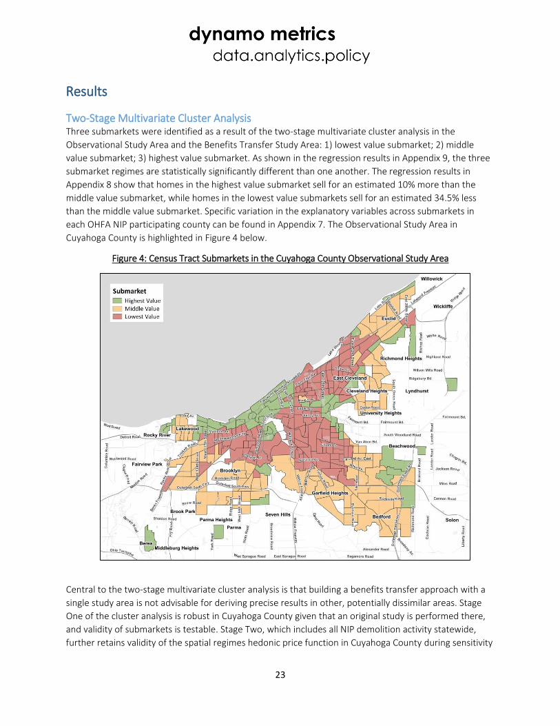
Two-Stage Multivariate Cluster Analysis Three submarkets were identified as a result of the two-stage multivariate cluster analysis in the
Observational Study Area and the Benefits Transfer Study Area: 1) lowest value submarket; 2) middle
value submarket; 3) highest value submarket. As shown in the regression results in Appendix 9, the three
submarket regimes are statistically significantly different than one another. The regression results in
Appendix 8 show that homes in the highest value submarket sell for an estimated 10% more than the
middle value submarket, while homes in the lowest value submarkets sell for an estimated 34.5% less
than the middle value submarket. Specific variation in the explanatory variables across submarkets in
each OHFA NIP participating county can be found in Appendix 7. The Observational Study Area in
Cuyahoga County is highlighted in Figure 4 below.
Figure 4: Census Tract Submarkets in the Cuyahoga County Observational Study Area
Central to the two-stage multivariate cluster analysis is that building a benefits transfer approach with a
single study area is not advisable for deriving precise results in other, potentially dissimilar areas. Stage
One of the cluster analysis is robust in Cuyahoga County given that an original study is performed there,
and validity of submarkets is testable. Stage Two, which includes all NIP demolition activity statewide,
further retains validity of the spatial regimes hedonic price function in Cuyahoga County during sensitivity
24
testing in terms of its predictive power and statistical significance.55 This means that the cluster analysis,
resultant submarkets and spatial regimes hedonic price function in Cuyahoga County is robust in its
definition of housing submarkets.
The Stage Two pooling in the cluster analysis provides some mixed results in the consistency of Census
Tract summary statistics at the individual county levels, as shown in Appendix 7. There is consistency in
the second stage method identifying the lowest market areas, but identifying a distinct difference
between the middle and highest value submarket varies in some cases. In short, the weakness of the
benefits transfer approach is exposed through the summary statistics at the county level. Using the
defined second stage submarket definitions in the Benefits Transfer Study Area is permissible despite
identified methodological weakness because of the following two assumptions: 1) OHFA NIP demolition
occurs in marginal and weak market neighborhoods; and, 2) the strength of previous studies in identifying
consistent confidence intervals related to blight impact on home value and vacant lot impact on home
value (i.e. home value impact rate available from demolition).56
Stage One Multivariate Cluster Analysis Results Based on 23 Census Tract level socio-economic and demographic variables57, Stage One of the two-stage
multivariate cluster analysis was run for the entirety of Cuyahoga County so the Observational Study Area
could be selected. Stage One selection of the Census Tract boundaries of the Observational Study Area
was based on identifying the best grouping of clusters that had at least one demolition occur within them,
and alike Census Tracts that did not have any demolition occur within them. A careful analysis revealed
that the optimal fit in Stage One included the k-means result with four housing submarkets. Census Tracts
where demolition occurred or were in the same clusters as those where demolition occurred fell into two
of the four clusters, which appear as green and grey within Appendix 3. These housing clusters were then
pooled with the rest of the Census Tracts across Ohio where OHFA NIP demolition occurred during the
study time period to prepare Stage Two of the cluster analysis. See Appendix 2 and 3 for detailed results
from the Stage One multivariate cluster analysis.
Stage Two Multivariate Cluster Analysis Based on the same 23 Census Tract level socio-economic and demographic variables from Stage One,
Stage Two of the analysis was run in the Observational Study Area identified in Stage One pooled with all
Census Tracts that received OHFA NIP demolition in the other 18 Ohio counties (the Benefits Transfer
Study Area). The result of the Stage Two analysis is the three submarkets assigned to each Census Tract in
the Observational Study Area for the hedonic modeling and benefits transfer analysis. Given that a
selection bias is imposed because only areas that had demolition or were like areas that had demolition
were included in the study, a “relative” naming convention for the housing submarket regimes is
required. This is because some of the areas where no demolition has occurred are the healthiest and
highest value housing markets, and these areas are effectively taken out of the study area in our
approach. The submarket naming convention is therefore “lowest,” “middle,” and “highest” value
55 See sensitivity testing results in Appendix 11.1 through 11.5. 56 See Immergluck (2015) 57 See Appendix 2 and 4 for a full listing of the 23 Census Tract variables used for the multivariate cluster analysis.
25
submarkets58, since they are relative to one another and not reflective of relative strength across the
entire Cuyahoga County housing market. Details of the Stage Two cluster analysis can be found in
Appendix 1.1-1.19 and Appendix 4. Summary statistics for all 23 variables used to perform the two-stage
cluster analysis associated with each submarket at the county level can be found in Appendix 7.
58 Given that housing and housing lot density is typically higher in the middle value market, the resulting BCR is highest there. While true, if the same density of the middle value market is available in a specific neighborhood the highest value market, then BCR would be much higher there because the housing value impact rate from demolition is over 18% in the highest value submarket and is 5.5% in the middle value market.
26
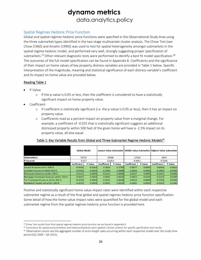
Spatial Regimes Hedonic Price Function Global and spatial regimes hedonic price functions were specified in the Observational Study Area using
the three submarket types identified in the two-stage multivariate cluster analysis. The Chow Test (see
Chow (1960) and Anselin (1990)) was used to test for spatial heterogeneity amongst submarkets in the
spatial regime hedonic model, and performed very well, strongly suggesting proper specification of
submarkets.59 Other relevant diagnostic tests were performed to identify a best fit model specification.60
The outcomes of the full model specification can be found in Appendix 8. Coefficients and the significance
of their impact on home values of key property distress variables are provided in Table 1 below. Specific
interpretation of the magnitude, meaning and statistical significance of each distress variable’s coefficient
and its impact on home value are provided below.
Reading Table 1
P-Value
o If the p-value is 0.05 or less, then the coefficient is considered to have a statistically
significant impact on home property value.
Coefficient
o If coefficient is statistically significant (i.e. the p-value is 0.05 or less), then it has an impact on
property value.
o Coefficients read as a percent impact on property value from a marginal change. For
example, a coefficient of -0.025 that is statistically significant suggests an additional
distressed property within 500 feet of the given home will have a -2.5% impact on its
property value, all else equal.
Table 1: Key Variable Results from Global and Three-Submarket Regime Hedonic Models61
Positive and statistically significant home value impact rates were identified within each respective
submarket regime as a result of the final global and spatial regimes hedonic price function specification.
Some detail of how the home value impact rates were quantified for the global model and each
submarket regime from the spatial regimes hedonic price function is provided here.
59 Chow Test results from final spatial regimes hedonic price function can be found in Appendix 9. 60 Corrections for spatial autocorrelation and heteroscedasticity were applied. Contact authors for specific specification test results. 61 Observation counts are the aggregate number of arms-length sales occurring within each respective model over the study time period (Q2 2009 – Q4 2015).
27
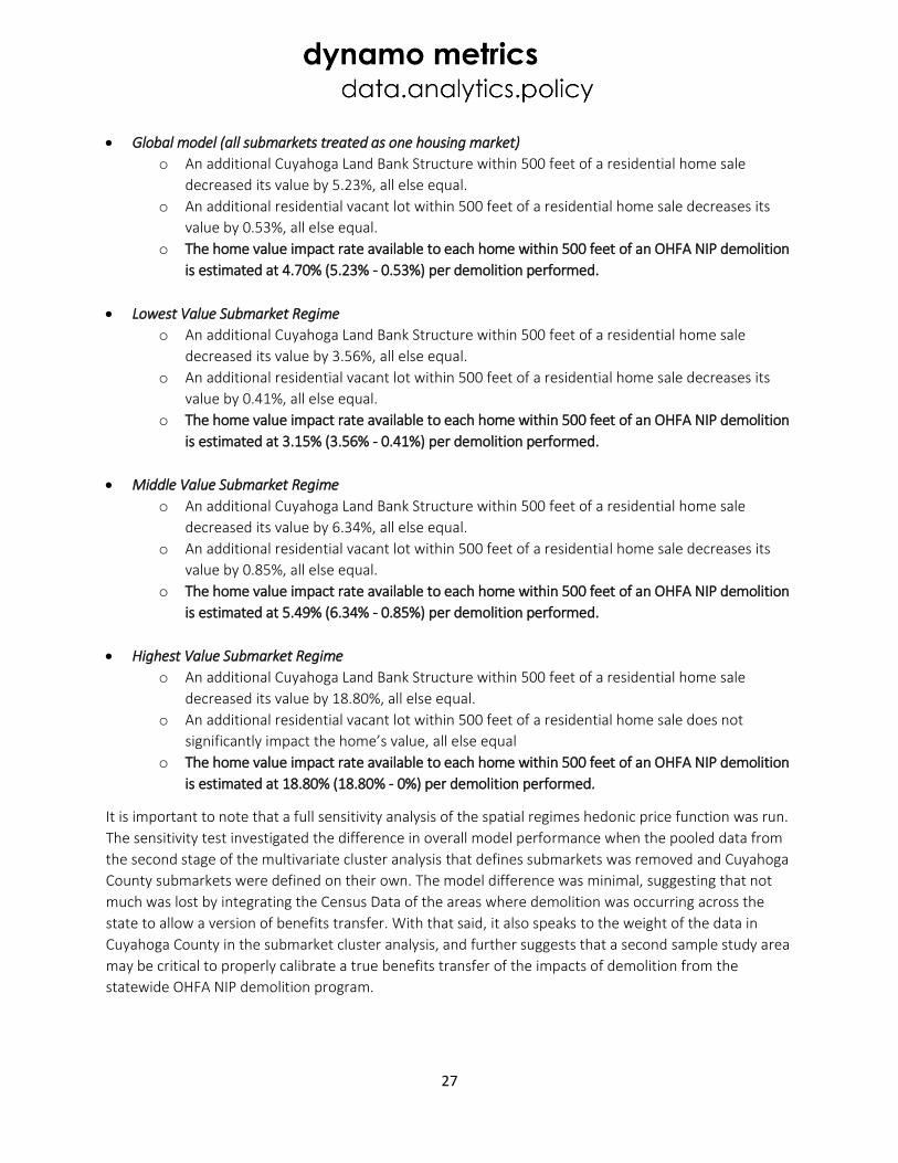
Global model (all submarkets treated as one housing market)
o An additional Cuyahoga Land Bank Structure within 500 feet of a residential home sale
decreased its value by 5.23%, all else equal.
o An additional residential vacant lot within 500 feet of a residential home sale decreases its
value by 0.53%, all else equal.
o The home value impact rate available to each home within 500 feet of an OHFA NIP demolition
is estimated at 4.70% (5.23% - 0.53%) per demolition performed.
Lowest Value Submarket Regime
o An additional Cuyahoga Land Bank Structure within 500 feet of a residential home sale
decreased its value by 3.56%, all else equal.
o An additional residential vacant lot within 500 feet of a residential home sale decreases its
value by 0.41%, all else equal.
o The home value impact rate available to each home within 500 feet of an OHFA NIP demolition
is estimated at 3.15% (3.56% - 0.41%) per demolition performed.
Middle Value Submarket Regime
o An additional Cuyahoga Land Bank Structure within 500 feet of a residential home sale
decreased its value by 6.34%, all else equal.
o An additional residential vacant lot within 500 feet of a residential home sale decreases its
value by 0.85%, all else equal.
o The home value impact rate available to each home within 500 feet of an OHFA NIP demolition
is estimated at 5.49% (6.34% - 0.85%) per demolition performed.
Highest Value Submarket Regime
o An additional Cuyahoga Land Bank Structure within 500 feet of a residential home sale
decreased its value by 18.80%, all else equal.
o An additional residential vacant lot within 500 feet of a residential home sale does not
significantly impact the home’s value, all else equal
o The home value impact rate available to each home within 500 feet of an OHFA NIP demolition
is estimated at 18.80% (18.80% - 0%) per demolition performed.
It is important to note that a full sensitivity analysis of the spatial regimes hedonic price function was run.
The sensitivity test investigated the difference in overall model performance when the pooled data from
the second stage of the multivariate cluster analysis that defines submarkets was removed and Cuyahoga
County submarkets were defined on their own. The model difference was minimal, suggesting that not
much was lost by integrating the Census Data of the areas where demolition was occurring across the
state to allow a version of benefits transfer. With that said, it also speaks to the weight of the data in
Cuyahoga County in the submarket cluster analysis, and further suggests that a second sample study area
may be critical to properly calibrate a true benefits transfer of the impacts of demolition from the
statewide OHFA NIP demolition program.
28
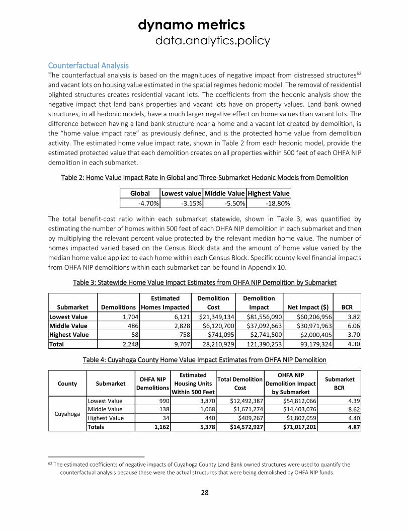
Counterfactual Analysis The counterfactual analysis is based on the magnitudes of negative impact from distressed structures62
and vacant lots on housing value estimated in the spatial regimes hedonic model. The removal of residential
blighted structures creates residential vacant lots. The coefficients from the hedonic analysis show the
negative impact that land bank properties and vacant lots have on property values. Land bank owned
structures, in all hedonic models, have a much larger negative effect on home values than vacant lots. The
difference between having a land bank structure near a home and a vacant lot created by demolition, is
the “home value impact rate” as previously defined, and is the protected home value from demolition
activity. The estimated home value impact rate, shown in Table 2 from each hedonic model, provide the
estimated protected value that each demolition creates on all properties within 500 feet of each OHFA NIP
demolition in each submarket.
Table 2: Home Value Impact Rate in Global and Three-Submarket Hedonic Models from Demolition
The total benefit-cost ratio within each submarket statewide, shown in Table 3, was quantified by
estimating the number of homes within 500 feet of each OHFA NIP demolition in each submarket and then
by multiplying the relevant percent value protected by the relevant median home value. The number of
homes impacted varied based on the Census Block data and the amount of home value varied by the
median home value applied to each home within each Census Block. Specific county level financial impacts
from OHFA NIP demolitions within each submarket can be found in Appendix 10.
Table 3: Statewide Home Value Impact Estimates from OHFA NIP Demolition by Submarket
Table 4: Cuyahoga County Home Value Impact Estimates from OHFA NIP Demolition
62 The estimated coefficients of negative impacts of Cuyahoga County Land Bank owned structures were used to quantify the
counterfactual analysis because these were the actual structures that were being demolished by OHFA NIP funds.
Global Lowest value Middle Value Highest Value
-4.70% -3.15% -5.50% -18.80%
Submarket Demolitions
Estimated
Homes Impacted
Demolition
Cost
Demolition
Impact Net Impact ($) BCR
Lowest Value 1,704 6,121 $21,349,134 $81,556,090 $60,206,956 3.82
Middle Value 486 2,828 $6,120,700 $37,092,663 $30,971,963 6.06
Highest Value 58 758 $741,095 $2,741,500 $2,000,405 3.70
Total 2,248 9,707 28,210,929 121,390,253 93,179,324 4.30
County SubmarketOHFA NIP
Demolitions
Estimated
Housing Units
Within 500 Feet
Total Demolition
Cost
OHFA NIP
Demolition Impact
by Submarket
Submarket
BCR
Lowest Value 990 3,870 $12,492,387 $54,812,066 4.39
Middle Value 138 1,068 $1,671,274 $14,403,076 8.62
Highest Value 34 440 $409,267 $1,802,059 4.40
Totals 1,162 5,378 $14,572,927 $71,017,201 4.87
Cuyahoga
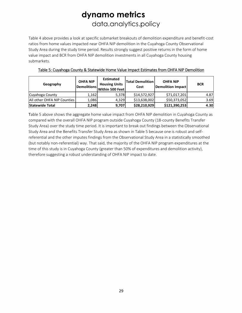
29
Table 4 above provides a look at specific submarket breakouts of demolition expenditure and benefit-cost
ratios from home values impacted near OHFA NIP demolition in the Cuyahoga County Observational
Study Area during the study time period. Results strongly suggest positive returns in the form of home
value impact and BCR from OHFA NIP demolition investments in all Cuyahoga County housing
submarkets.
Table 5: Cuyahoga County & Statewide Home Value Impact Estimates from OHFA NIP Demolition
Table 5 above shows the aggregate home value impact from OHFA NIP demolition in Cuyahoga County as
compared with the overall OHFA NIP program outside Cuyahoga County (18-county Benefits Transfer
Study Area) over the study time period. It is important to break out findings between the Observational
Study Area and the Benefits Transfer Study Area as shown in Table 5 because one is robust and self-
referential and the other imputes findings from the Observational Study Area in a statistically smoothed
(but notably non-referential) way. That said, the majority of the OHFA NIP program expenditures at the
time of this study is in Cuyahoga County (greater than 50% of expenditures and demolition activity),
therefore suggesting a robust understanding of OHFA NIP impact to date.
GeographyOHFA NIP
Demolitions
Estimated
Housing Units
Within 500 Feet
Total Demolition
Cost
OHFA NIP
Demolition Impact BCR
Cuyahoga County 1,162 5,378 $14,572,927 $71,017,201 4.87
All other OHFA NIP Counties 1,086 4,329 $13,638,002 $50,373,052 3.69
Statewide Total 2,248 9,707 $28,210,929 $121,390,253 4.30
30
Comparative Trends Analysis The comparative trends analysis provides a view into the strength of the relationship between demolition
activity in Cuyahoga County and homeownership preservation as expressed through localized mortgage
foreclosure rates over time. Primarily designed for decision support,63a visual analysis of the trends shows
favorable relationships of the impact of demolition on mortgage foreclosure rates over time in all
comparative zones – meaning that trend lines of areas receiving demolition are either lower or
decreasing at a faster rate than areas without demolition, or both. Paired difference in means t-tests
were performed on the differing mortgage foreclosure rates in the aggregate and three submarkets
within the Observational Study Area. The only t-test that showed a statistically significant difference
between mortgage foreclosure rates where demolition has and has not occurred is the middle value
housing submarket.64 The results of this analysis within each submarket are graphed below.
63 Parallel analysis used for decision support by U.S. Treasury can be found in Griswold et al., 2014. 64 Middle value submarket paired t-test score was statistically significant at the 0.000 level.
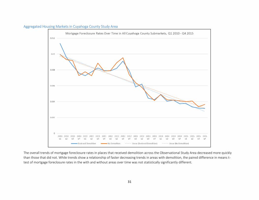
31
Aggregated Housing Markets in Cuyahoga County Study Area
The overall trends of mortgage foreclosure rates in places that received demolition across the Observational Study Area decreased more quickly
than those that did not. While trends show a relationship of faster decreasing trends in areas with demolition, the paired difference in means t-
test of mortgage foreclosure rates in the with and without areas over time was not statistically significantly different.
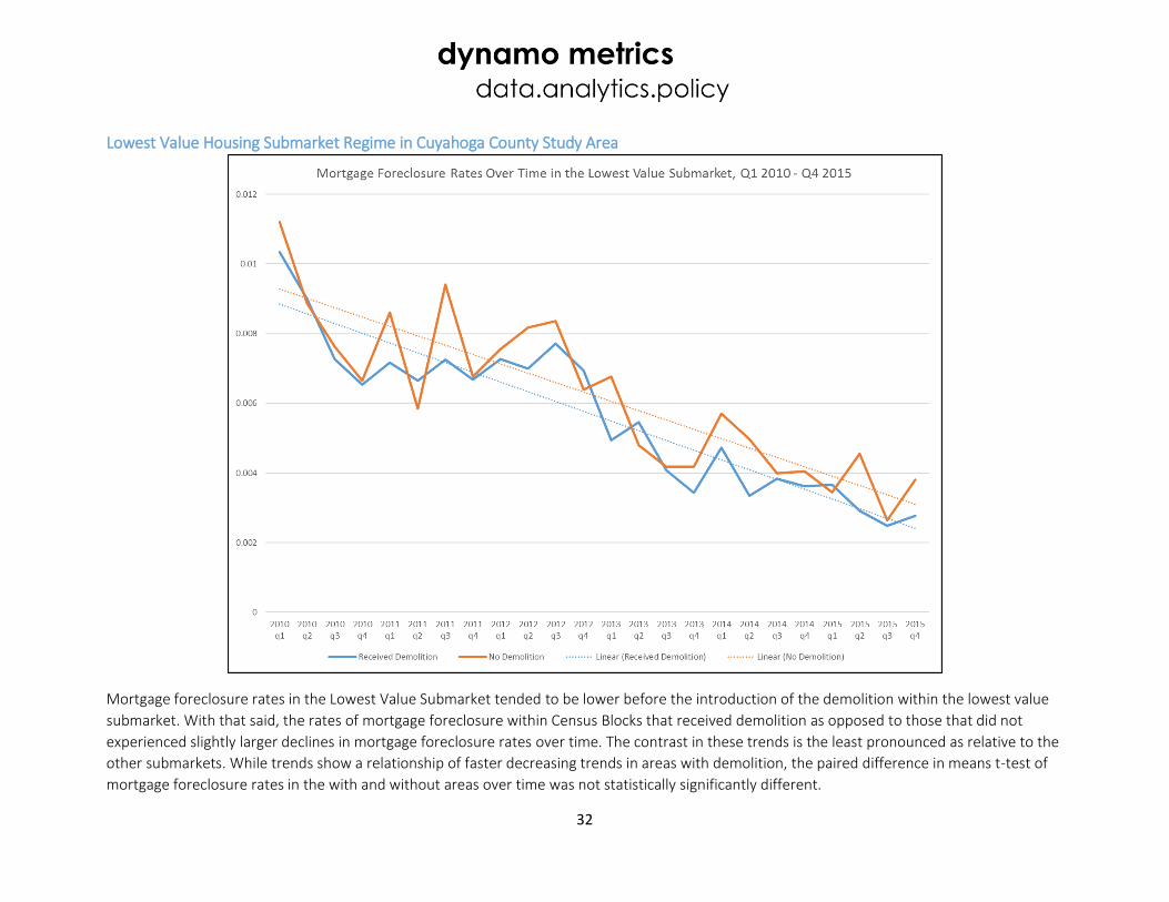
32
Lowest Value Housing Submarket Regime in Cuyahoga County Study Area
Mortgage foreclosure rates in the Lowest Value Submarket tended to be lower before the introduction of the demolition within the lowest value
submarket. With that said, the rates of mortgage foreclosure within Census Blocks that received demolition as opposed to those that did not
experienced slightly larger declines in mortgage foreclosure rates over time. The contrast in these trends is the least pronounced as relative to the
other submarkets. While trends show a relationship of faster decreasing trends in areas with demolition, the paired difference in means t-test of
mortgage foreclosure rates in the with and without areas over time was not statistically significantly different.
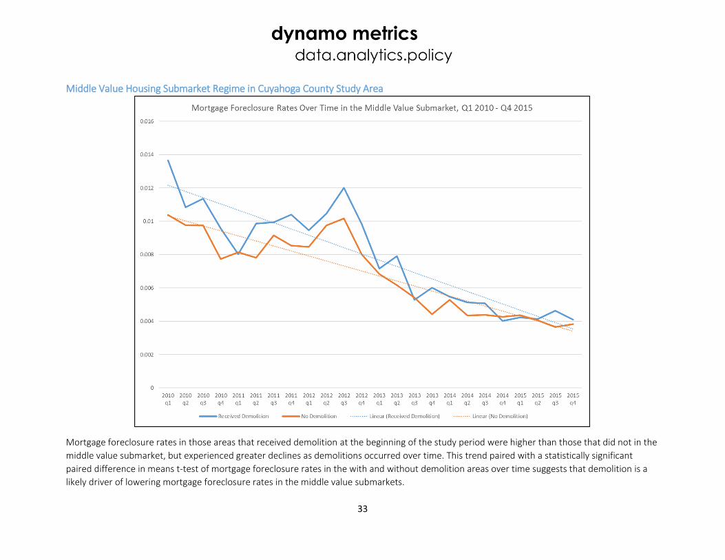
33
Middle Value Housing Submarket Regime in Cuyahoga County Study Area
Mortgage foreclosure rates in those areas that received demolition at the beginning of the study period were higher than those that did not in the
middle value submarket, but experienced greater declines as demolitions occurred over time. This trend paired with a statistically significant
paired difference in means t-test of mortgage foreclosure rates in the with and without demolition areas over time suggests that demolition is a
likely driver of lowering mortgage foreclosure rates in the middle value submarkets.
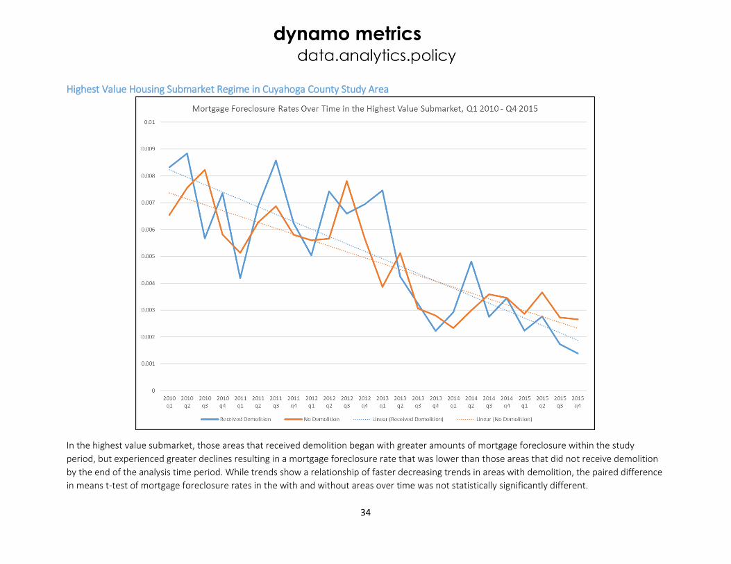
34
Highest Value Housing Submarket Regime in Cuyahoga County Study Area
In the highest value submarket, those areas that received demolition began with greater amounts of mortgage foreclosure within the study
period, but experienced greater declines resulting in a mortgage foreclosure rate that was lower than those areas that did not receive demolition
by the end of the analysis time period. While trends show a relationship of faster decreasing trends in areas with demolition, the paired difference
in means t-test of mortgage foreclosure rates in the with and without areas over time was not statistically significantly different.
35
Study Discussion 1. For the first time in spatial econometric distressed property research, the impact of county land bank
owned structures was differentiated from other distressed structure typologies. The county land bank owned structures consistently had the highest negative impact on nearby housing in every submarket regime. We did not differentiate between structures headed for demolition, on the one hand, and structures headed for rehabilitation, resale, or mothballing on the other hand. Nor are we suggesting that county land banks are bad landlords; it is merely the properties that they hold naturally tend to have blight characteristics. Presuming that the county land banks acquire some better condition properties with an eye toward rehabilitation, it may be inferred that this study actually underestimates the negative impact of county land bank owned properties acquired for demolition. The home value impact rates might have been larger had the study differentiated between the two land bank property types as described above.
2. A selection bias was introduced in the spatial regimes hedonic price function that does not allow housing sales observations within the final model that are not in the Observation Study Area. This bias was purposely introduced in an attempt to isolate the demolition impact investigation into areas where demolition is actually occurring or are similar to areas where demolition is occurring. The naming convention attached to the housing submarkets is therefore relative – highest, middle and lowest value submarkets, because the markets where no demolition is occurring (likely more stable and higher value) are omitted. This speaks to the insight that demolition tends to occur in weak and marginal markets. Statistics of the hedonic model observations are such that 75% of sales were priced below $65,000 and 50% of sales observations were priced below $30,000. The healthiest housing markets in Cuyahoga County are therefore not readily observed in this study.
3. Some of the time periods used in the occurred prior to the OHFA NIP specific time periods. Previous periods were used because, in hedonic modeling, a deeper time series best specifies robust coefficient estimates in the key distress variables. These robust distress variable coefficient estimates were used as multipliers in the counterfactual analysis for all OHFA NIP demolitions, and are applicable beyond the Q4 2015-time period of the model specification – therefore allowing demolition in 2016 to be considered in the counterfactual analysis.
4. This study quantifies and assesses the beneficial impacts of OHFA NIP demolition during a specific slice of time (Q1 2014 – Q1 2016). Given planned blight removal programming through 2020, this research serves as the basis for identifying all Census Tract-level submarkets (only Census Tracts where demolition occurred to date we included in this study), and therefore the demolition benefit multipliers in all participating and potentially participating county Census Tracts. Such fully-developed targeting of impacts is consistent with EESA’s goal of maximizing the taxpayers’ return on HHF investment.
36
Discussion of Benefits Transfer Analysis 5. The benefits transfer approach used in this study is its primary limitation or weakness. Taking into
account both time and resource constraints associated with this study, the benefits transfer method used in this context is a new contribution towards identifying effective methods of imputing demolition impact results from one regional economy’s submarkets to another’s. It also is an innovation towards providing near real-time decision support for future action. With that said, the transferability of the results of the benefits estimation from the spatial regimes hedonic price function from the Observational Study Area to the 18 other Ohio areas rests on two assumptions:
The submarket structure identified through the cluster analysis on the principal components of the Census Tract variables for the Census Tracts identified in the sample is representative for each of the relevant areas in the 18 other counties over the time period covering the study;
The regression results (the coefficient estimates) that were obtained from the in-depth analysis of the Cuyahoga County observational study area housing market apply to the benefits transfer study area housing markets of the relevant areas in the 18 other counties.
The first assumption is addressed by pooling census observations for all Census Tracts in Ohio where
demolition activity occurred (Stage Two of the cluster analysis) with the Census Tracts in the Cuyahoga
County sample. Initial examination of the results showed that a cluster analysis for Cuyahoga County by
itself revealed similar groupings as those obtained from the full data set.65 However, this does not
necessarily imply that the reverse holds as well. This would require a separate clustering exercise for
representative Census Tracts in each of the 18 counties (not just Census Tracts with demolition activity)
and an assessment of the degree to which they conform to the patterns suggested by the pooled data. If
the socio-economic makeup of the 18 counties is similar enough, the first assumption is reasonable.
However, there are grounds to suspect that Cuyahoga County may not be fully representative of the
others due to the broad range of housing variability there. The only objective way to assess this is by
means of a separate analysis for each of the 18 areas. In addition, the submarket determination is based
on Census data at one point in time. To the extent that the socio-economic makeup of some of the
subareas may be changing over time, this would also need to be accounted for.66
The second assumption is more tenuous. It boils down to accepting that the structural characteristics of
the housing submarkets in the Census Tracts within the 18 counties in question are identical to those of
the Cuyahoga County housing submarkets under investigation. This is necessarily wrong to some extent.
The extent to which it does not hold will affect the degree of precision that can be attributed to the
overall benefit estimate that is extrapolated to the areas not included in the econometric analysis. The
only solid way to turn this unproven assumption into more reliable findings would be to conduct separate
and similar analyses for each of the 18 counties As an intermediate solution, a separate analysis in a
second urban county could provide a formal basis for extrapolation of the degree to which the estimates
in the second study county deviates from the estimates in a first (e.g., Cuyahoga County), and how such
deviation could be related to measureable characteristics of the area (e.g., unemployment rate, number
of housing starts).67
65 Compare findings in Appendix 1.5 with 11.2 to examine these differences. 66 See Mikelbank (2011) for discussion of neighborhood dynamics from 1970-2000 in Cleveland, OH. 67 See Footnote 31 for discussion regarding how the assumptions in this section were addressed in this study.
37
Key Insights 1. As shown in Appendix 10 and elsewhere, OHFA NIP appears to be meeting the EESA objective of
protecting home values in all housing submarkets.
2. In terms of homeownership preservation, evidence is strongest that mortgage foreclosure rates are decreasing faster in areas receiving demolition than in areas not receiving demolition in the middle value submarket. While the comparative trends are favorable toward a similar conclusion in the other submarket comparative trends analyses, the trend lines are not shown to be statistically significantly different than one another in those housing markets. This suggests that conducting as many demolitions as possible in the middle value (“yellow” in Appendix 1.5) submarket will do the most to reduce mortgage foreclosure rates over time.
3. A recurrent insight from previous demolition impact studies that continues to be drawn from this study is that evidence shows demolition activity having the largest impact when it occurs at the margin of neighborhood health. The greatest benefit-cost ratio in the Cuyahoga County Observational Study Area is found in the middle value submarket ($8.62 in home value protected for each $1 in demolition cost) – almost double the benefit-cost ratio of either the lowest value submarket ($4.39 value retained to $1 cost) or the highest value submarket ($4.40 value retained to $1 cost). This suggests that conducting as many demolitions as possible in the middle value (“yellow” in Appendix 1.5) submarket will preserve the most home value.68 Further, and as noted in Paragraph 2, above, the middle value submarket comparative trend analysis is the only submarket that shows mortgage foreclosure rates over time in areas that received demolition are statistically significantly decreasing faster than areas that did not receive demolition. Both parts of this study suggest that identifying areas within cities where the housing market is poised for positive or negative change in neighborhood health (i.e. the “margin” of the housing market) is key intelligence for decision making related to publicly funded housing market intervention.69
4. A new finding from the study provides evidence that more than a decade of high volume demolition activity is likely stabilizing the lowest value housing submarkets of the Cuyahoga County Observational Study Area. Given sustained demolition in Cuyahoga County, a statistically significant home value impact rate of 3.15% is identified from demolition in these areas. This hedge was not present in a parallel study performed three years ago.70
68 See footnote 58 on page 25 for further discussion related to relative housing density in the middle and highest value submarkets and how lot density impacts the BCR in those submarkets. 69 For precision application, on-the-ground targeting would identify optimally impactful demolition sites at the property level by taking housing submarket, housing values in the immediate area, and the relative housing density surrounding each potential location into account given that optimal impact occurs where the highest submarket multiplier, highest home values and highest housing density exist simultaneously. 70 See Griswold et al. (2014).
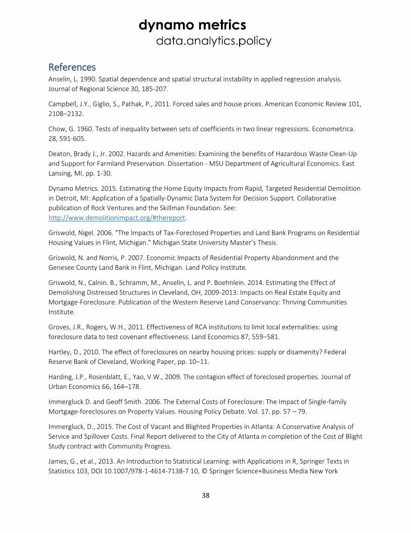
38
References Anselin, L. 1990. Spatial dependence and spatial structural instability in applied regression analysis.
Journal of Regional Science 30, 185-207.
Campbell, J.Y., Giglio, S., Pathak, P., 2011. Forced sales and house prices. American Economic Review 101,
2108–2132.
Chow, G. 1960. Tests of inequality between sets of coefficients in two linear regressions. Econometrica.
28, 591-605.
Deaton, Brady J., Jr. 2002. Hazards and Amenities: Examining the benefits of Hazardous Waste Clean-Up
and Support for Farmland Preservation. Dissertation - MSU Department of Agricultural Economics. East
Lansing, MI. pp. 1-30.
Dynamo Metrics. 2015. Estimating the Home Equity Impacts from Rapid, Targeted Residential Demolition
in Detroit, MI: Application of a Spatially-Dynamic Data System for Decision Support. Collaborative
publication of Rock Ventures and the Skillman Foundation. See:
http://www.demolitionimpact.org/#thereport.
Griswold, Nigel. 2006. "The Impacts of Tax-Foreclosed Properties and Land Bank Programs on Residential
Housing Values in Flint, Michigan." Michigan State University Master’s Thesis.
Griswold, N. and Norris, P. 2007. Economic Impacts of Residential Property Abandonment and the
Genesee County Land Bank in Flint, Michigan. Land Policy Institute.
Griswold, N., Calnin. B., Schramm, M., Anselin, L. and P. Boehnlein. 2014. Estimating the Effect of
Demolishing Distressed Structures in Cleveland, OH, 2009-2013: Impacts on Real Estate Equity and
Mortgage-Foreclosure. Publication of the Western Reserve Land Conservancy: Thriving Communities
Institute.
Groves, J.R., Rogers, W.H., 2011. Effectiveness of RCA institutions to limit local externalities: using
foreclosure data to test covenant effectiveness. Land Economics 87, 559–581.
Hartley, D., 2010. The effect of foreclosures on nearby housing prices: supply or disamenity? Federal
Reserve Bank of Cleveland, Working Paper, pp. 10–11.
Harding, J.P., Rosenblatt, E., Yao, V.W., 2009. The contagion effect of foreclosed properties. Journal of
Urban Economics 66, 164–178.
Immergluck D. and Geoff Smith. 2006. The External Costs of Foreclosure: The Impact of Single-family
Mortgage-foreclosures on Property Values. Housing Policy Debate. Vol. 17. pp. 57 – 79.
Immergluck, D., 2015. The Cost of Vacant and Blighted Properties in Atlanta: A Conservative Analysis of
Service and Spillover Costs. Final Report delivered to the City of Atlanta in completion of the Cost of Blight
Study contract with Community Progress.
James, G., et al., 2013. An Introduction to Statistical Learning: with Applications in R, Springer Texts in
Statistics 103, DOI 10.1007/978-1-4614-7138-7 10, © Springer Science+Business Media New York
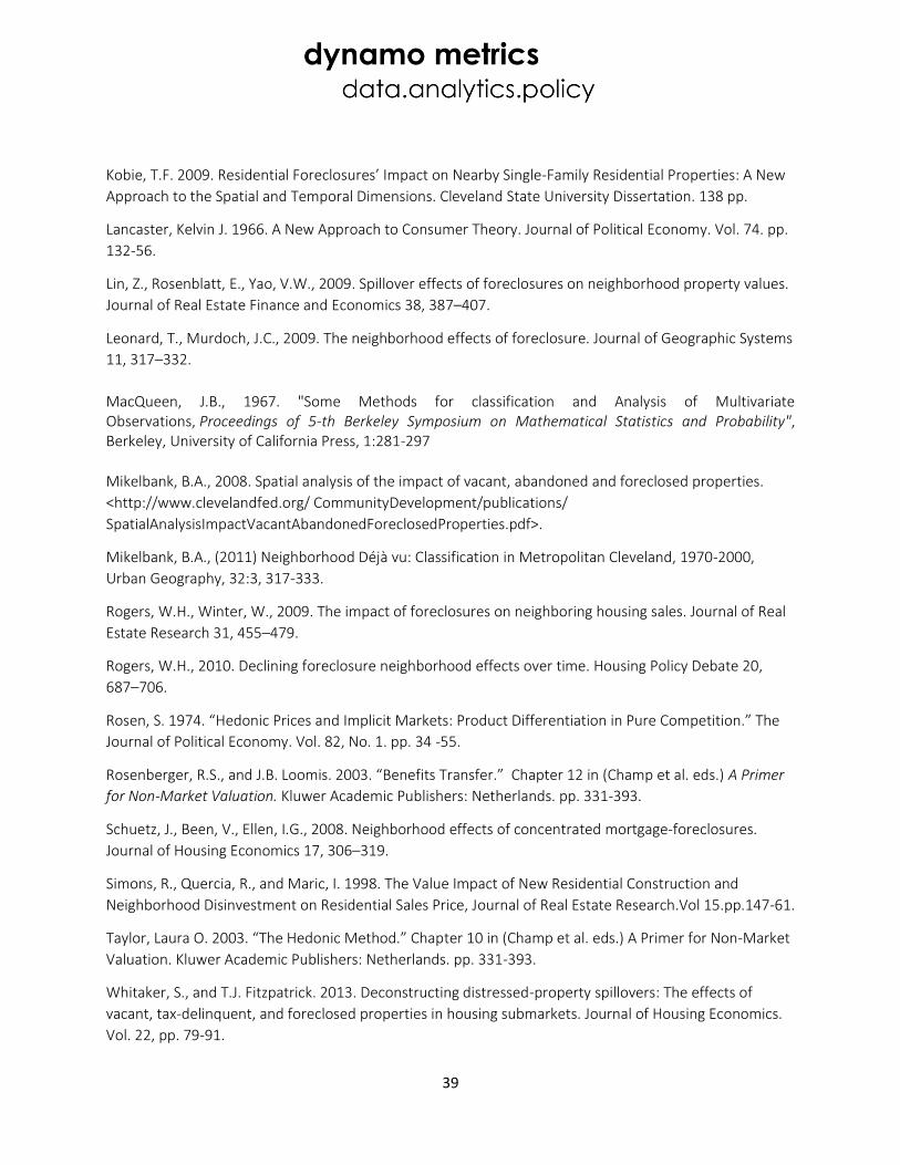
39
Kobie, T.F. 2009. Residential Foreclosures’ Impact on Nearby Single-Family Residential Properties: A New
Approach to the Spatial and Temporal Dimensions. Cleveland State University Dissertation. 138 pp.
Lancaster, Kelvin J. 1966. A New Approach to Consumer Theory. Journal of Political Economy. Vol. 74. pp.
132-56.
Lin, Z., Rosenblatt, E., Yao, V.W., 2009. Spillover effects of foreclosures on neighborhood property values.
Journal of Real Estate Finance and Economics 38, 387–407.
Leonard, T., Murdoch, J.C., 2009. The neighborhood effects of foreclosure. Journal of Geographic Systems
11, 317–332.
MacQueen, J.B., 1967. "Some Methods for classification and Analysis of Multivariate Observations, Proceedings of 5-th Berkeley Symposium on Mathematical Statistics and Probability", Berkeley, University of California Press, 1:281-297
Mikelbank, B.A., 2008. Spatial analysis of the impact of vacant, abandoned and foreclosed properties.
<http://www.clevelandfed.org/ CommunityDevelopment/publications/
SpatialAnalysisImpactVacantAbandonedForeclosedProperties.pdf>.
Mikelbank, B.A., (2011) Neighborhood Déjà vu: Classification in Metropolitan Cleveland, 1970-2000,
Urban Geography, 32:3, 317-333.
Rogers, W.H., Winter, W., 2009. The impact of foreclosures on neighboring housing sales. Journal of Real
Estate Research 31, 455–479.
Rogers, W.H., 2010. Declining foreclosure neighborhood effects over time. Housing Policy Debate 20,
687–706.
Rosen, S. 1974. “Hedonic Prices and Implicit Markets: Product Differentiation in Pure Competition.” The
Journal of Political Economy. Vol. 82, No. 1. pp. 34 -55.
Rosenberger, R.S., and J.B. Loomis. 2003. “Benefits Transfer.” Chapter 12 in (Champ et al. eds.) A Primer
for Non-Market Valuation. Kluwer Academic Publishers: Netherlands. pp. 331-393.
Schuetz, J., Been, V., Ellen, I.G., 2008. Neighborhood effects of concentrated mortgage-foreclosures.
Journal of Housing Economics 17, 306–319.
Simons, R., Quercia, R., and Maric, I. 1998. The Value Impact of New Residential Construction and
Neighborhood Disinvestment on Residential Sales Price, Journal of Real Estate Research.Vol 15.pp.147-61.
Taylor, Laura O. 2003. “The Hedonic Method.” Chapter 10 in (Champ et al. eds.) A Primer for Non-Market
Valuation. Kluwer Academic Publishers: Netherlands. pp. 331-393.
Whitaker, S., and T.J. Fitzpatrick. 2013. Deconstructing distressed-property spillovers: The effects of
vacant, tax-delinquent, and foreclosed properties in housing submarkets. Journal of Housing Economics.
Vol. 22, pp. 79-91.
40
Appendix 1: Stage 2 K-Means Clustering Results for Statewide OHFA NIP
County Submarkets
Appendix 1.1: Ashtabula County OHFA NIP Submarkets
41
Appendix 1.2: Butler County OHFA NIP Submarkets

42
Appendix 1.3: Clark County OHFA NIP Submarkets
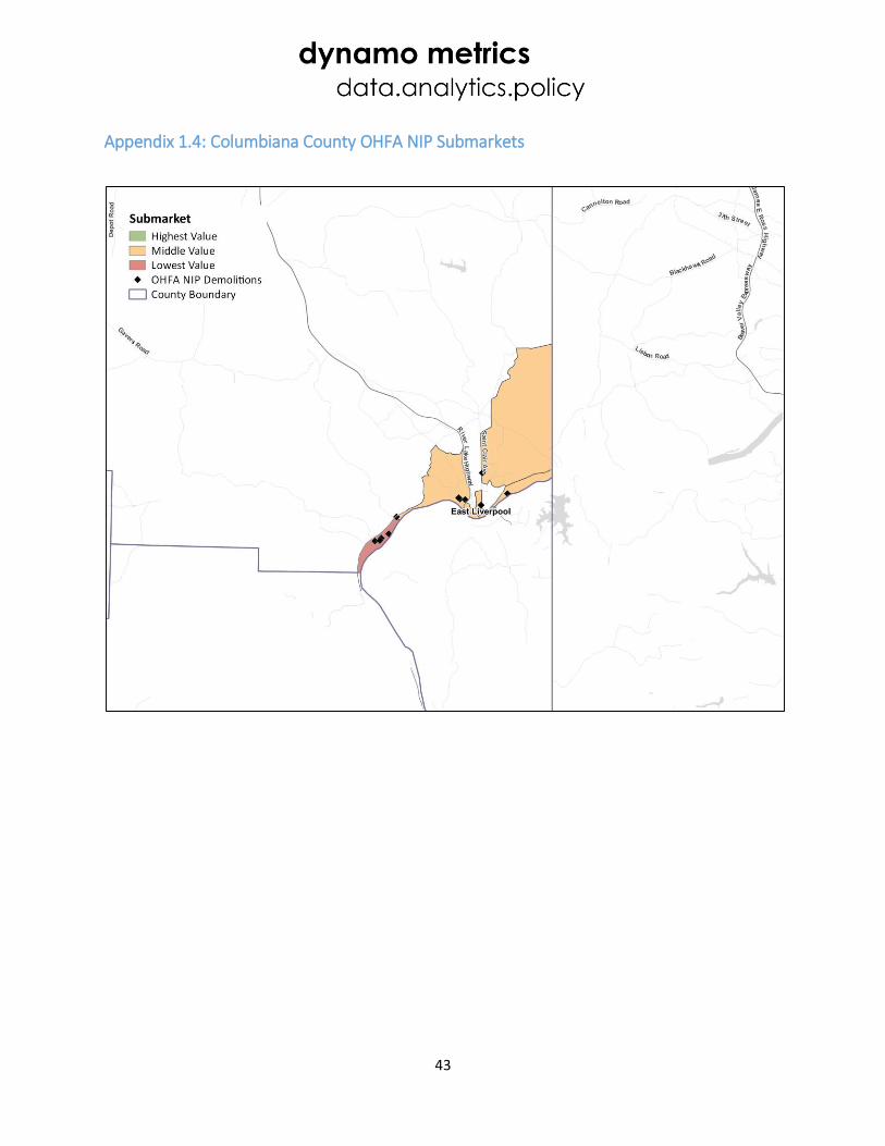
43
Appendix 1.4: Columbiana County OHFA NIP Submarkets
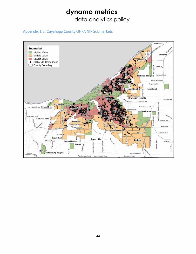
44
Appendix 1.5: Cuyahoga County OHFA NIP Submarkets
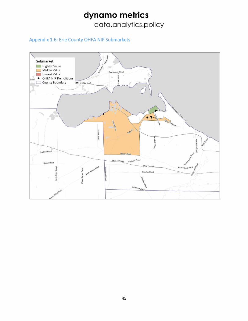
45
Appendix 1.6: Erie County OHFA NIP Submarkets

46
Appendix 1.7: Fairfield County OHFA NIP Submarkets
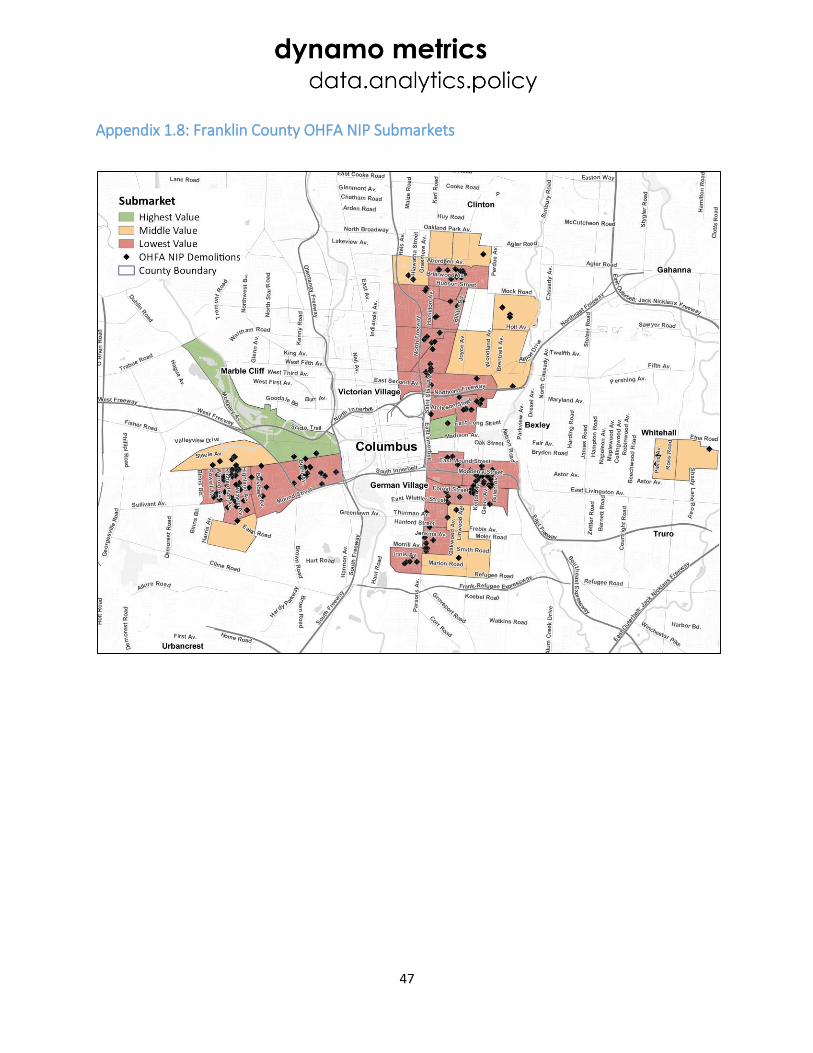
47
Appendix 1.8: Franklin County OHFA NIP Submarkets
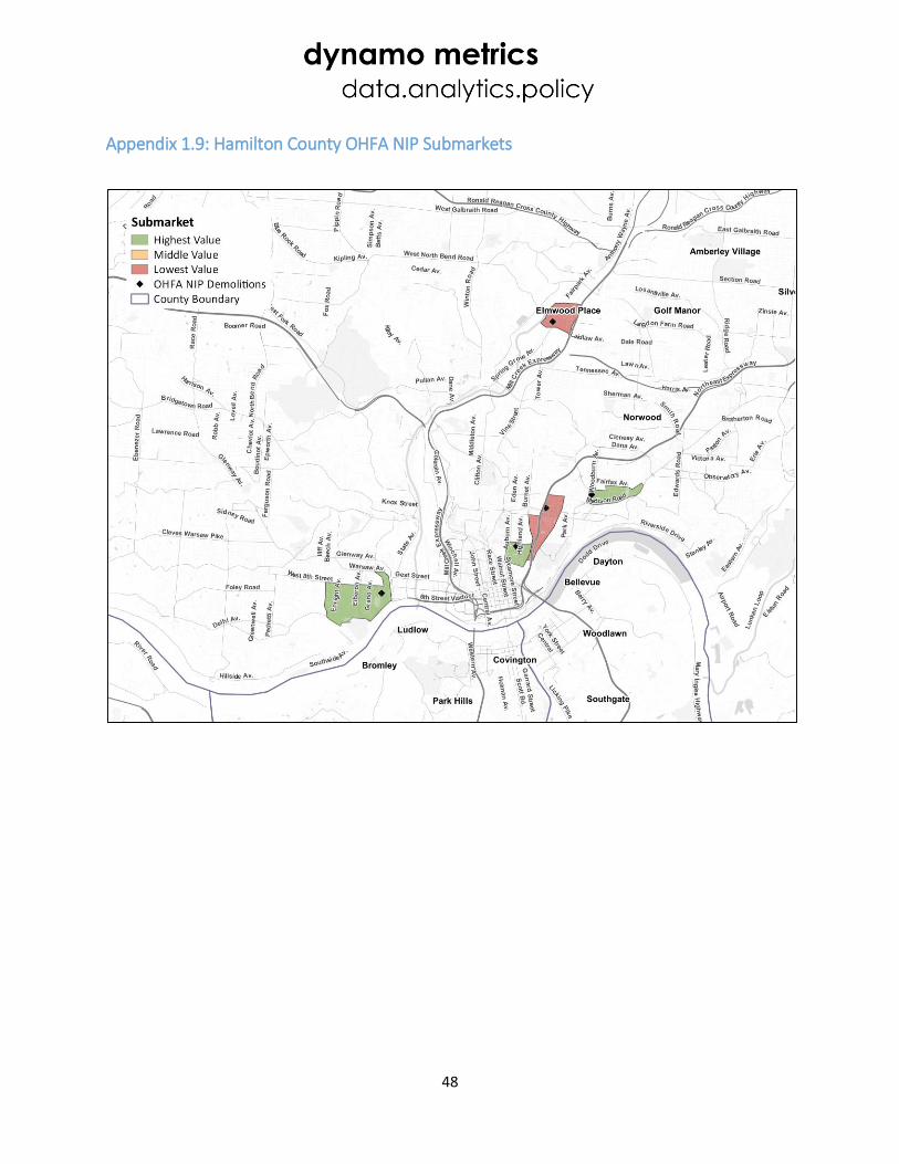
48
Appendix 1.9: Hamilton County OHFA NIP Submarkets
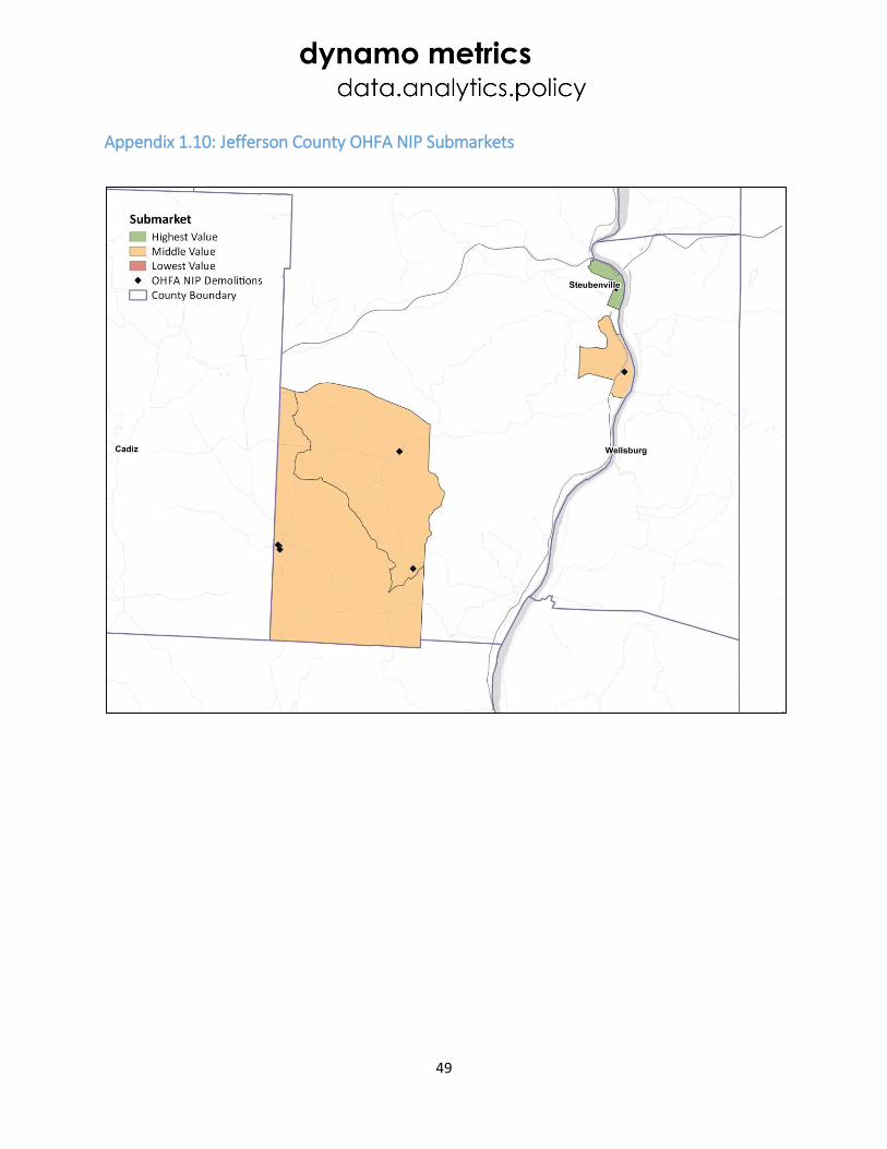
49
Appendix 1.10: Jefferson County OHFA NIP Submarkets

50
Appendix 1.11: Lake County OHFA NIP Submarkets
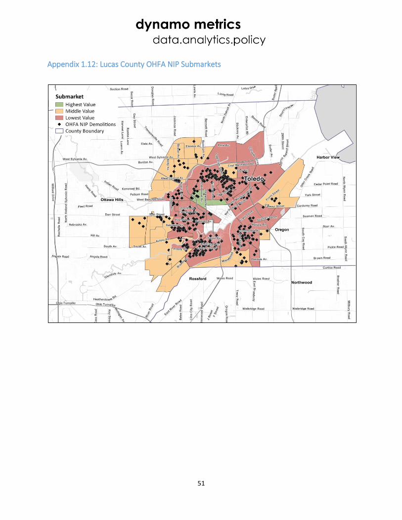
51
Appendix 1.12: Lucas County OHFA NIP Submarkets
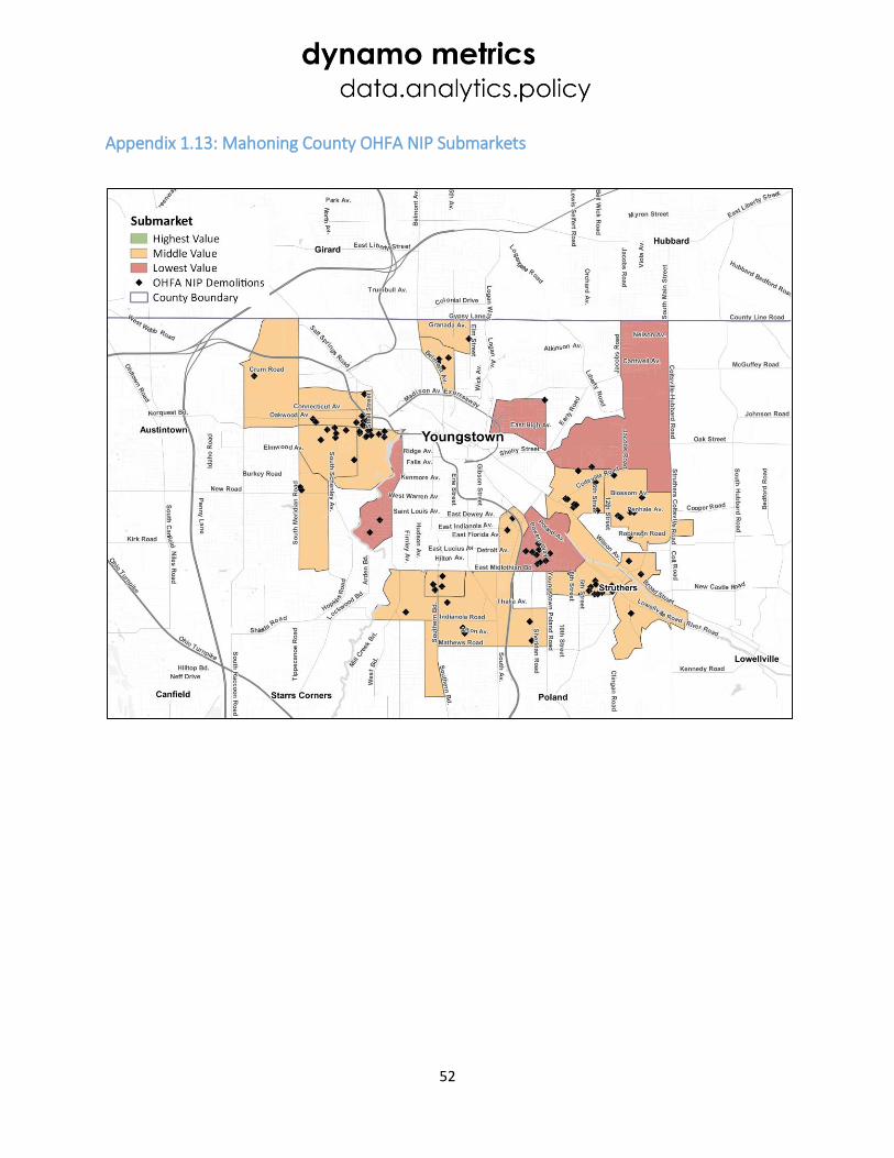
52
Appendix 1.13: Mahoning County OHFA NIP Submarkets
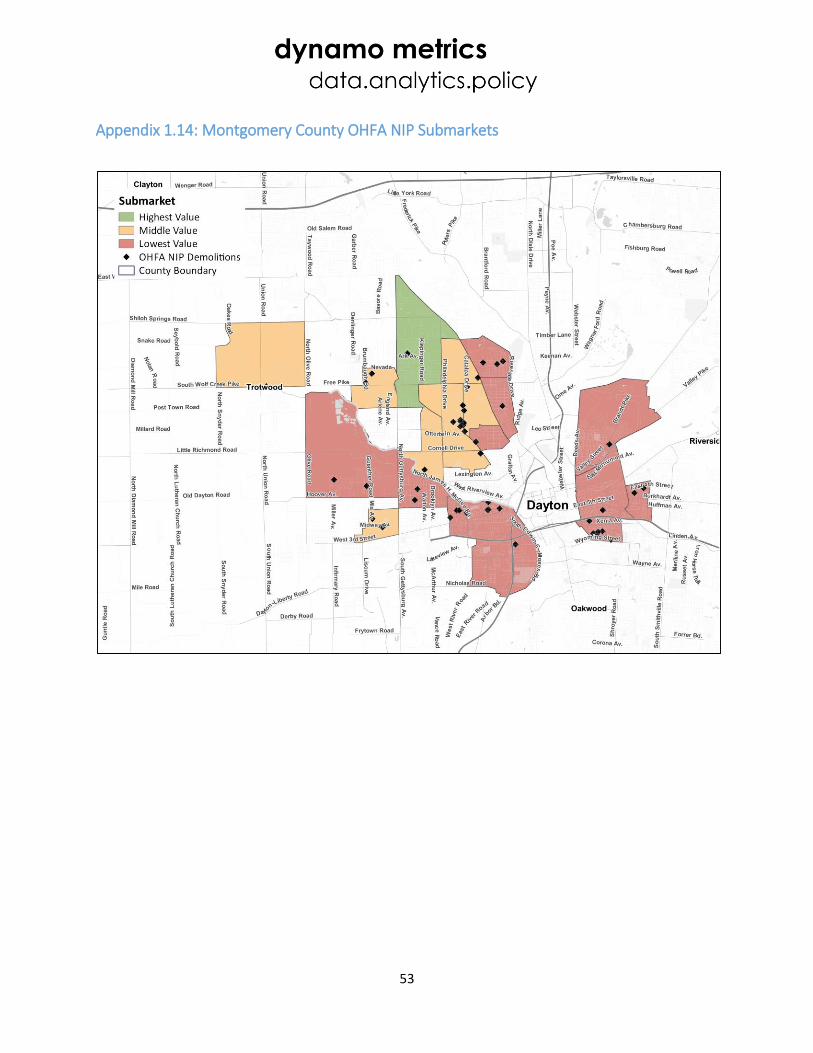
53
Appendix 1.14: Montgomery County OHFA NIP Submarkets
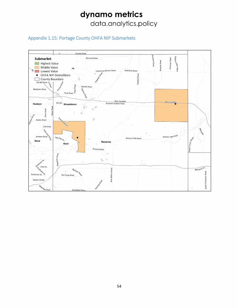
54
Appendix 1.15: Portage County OHFA NIP Submarkets
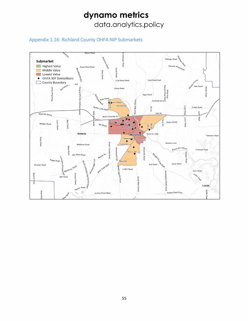
55
Appendix 1.16: Richland County OHFA NIP Submarkets
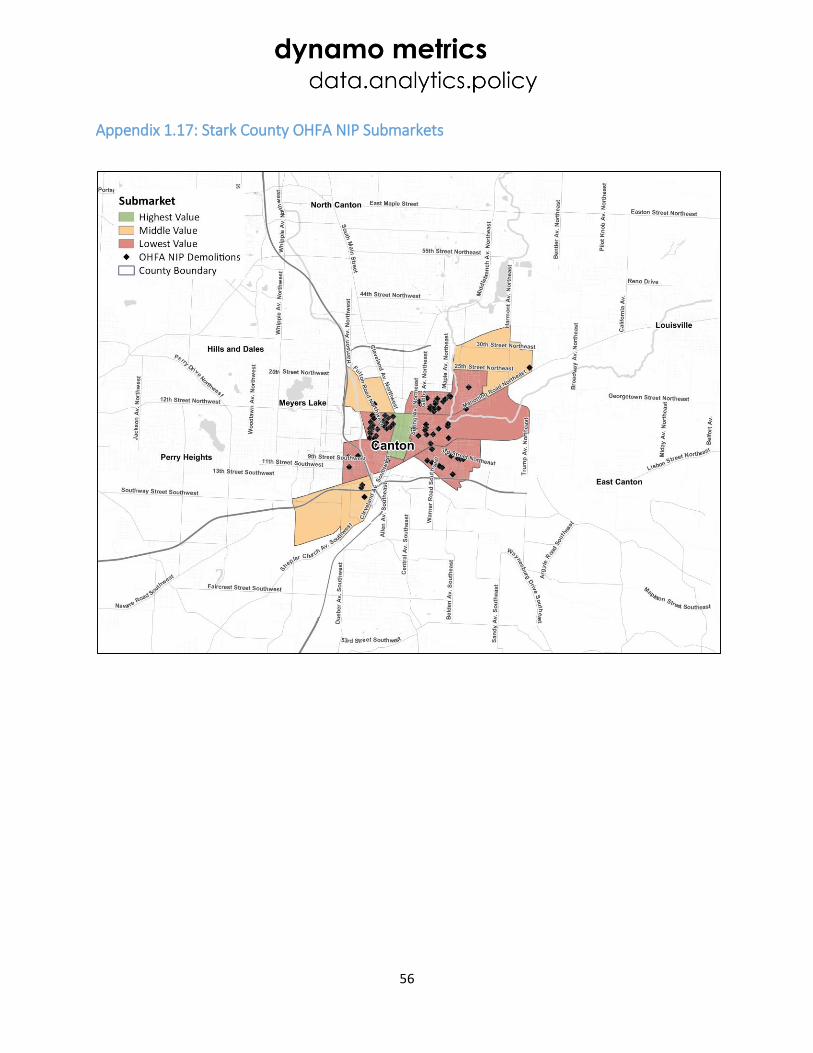
56
Appendix 1.17: Stark County OHFA NIP Submarkets

57
Appendix 1.18: Summit County OHFA NIP Submarkets
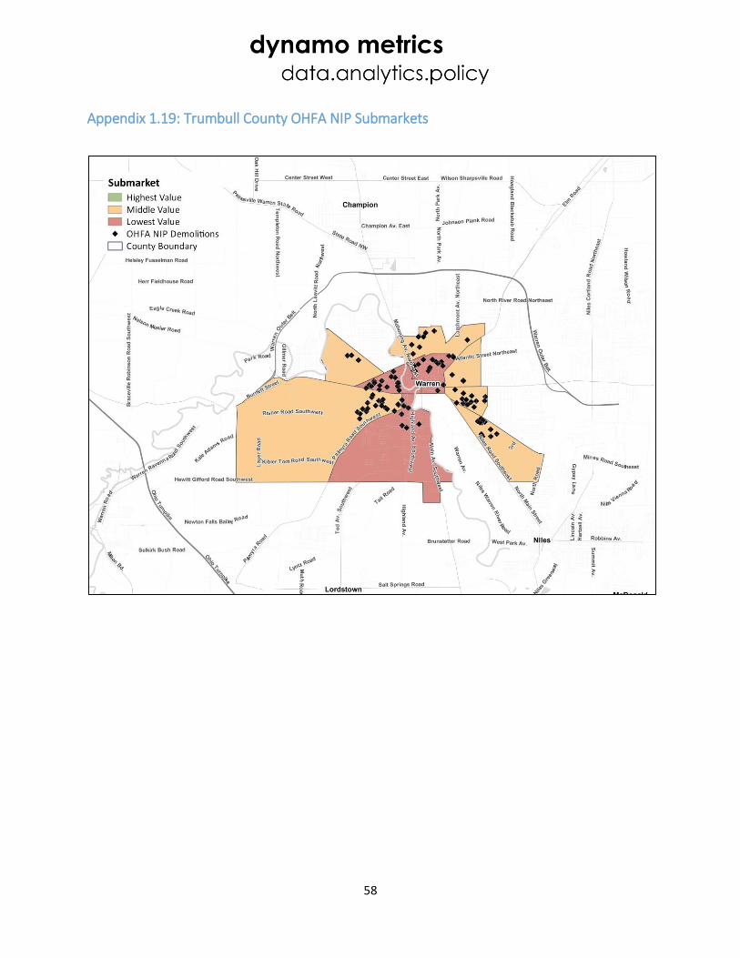
58
Appendix 1.19: Trumbull County OHFA NIP Submarkets

59
Appendix 2: Stage 1 Principal Components Analysis Results
As shown in the far right column, the first two components of the PCA explain 50.85% of the variation in
the 23 Census Tract variables in Cuyahoga County.
As shown in the scree plot above, a decisive “elbow” effect is graphed in the Eigenvalues of the PCA,
suggesting the first two components are strongly representative weighted mixes of the 23 Census Tract
variables.
Principle Components Eigenvalue Difference Proportion Cumulative
Component 1 8.96457 6.23406 0.3898 0.3898
Component 2 2.73051 0.439991 0.1187 0.5085
Stage 1 Principle Components Analysis: Cuyahoga County

60
The relative weightings of the first two components of the PCA are shown for all 23 Census Tract variables
taken into account in Cuyahoga County. Component 1 is most strongly loaded in socio-demographic
variables while the Component 2 is more strongly loaded in its weightings on housing variables.
Census Tract Level Variable Component 1 Component 2
Population per Square Mile -0.1741 0.0234
Median Household Income 0.3050 0.1686
Median Rent 0.2271 0.0885
Median Home Value 0.2731 0.1825
% Unoccupied -0.2590 0.1388
% Owner Occupied 0.2679 0.0101
% High School Diploma 0.2742 -0.0589
% Bachelor's Degree 0.2629 0.1351
% Poverty -0.2978 0.1161
% Unemployment -0.2703 0.1257
% 2-3 Bedrooms -0.0867 -0.2573
% 4 Bedrooms or More 0.1894 0.4116
% Homes Built 2000 - Present 0.0144 0.1903
% Homes Built 1980 - 1999 0.1557 0.1276
% Homes Built 1960 - 1979 0.1548 -0.2597
% Homes Built 1940 - 1959 0.0530 -0.2771
% Homes Built 1939 and Earlier -0.2106 0.2461
Average Household Size 0.0461 0.4009
% Kids 18 and Under -0.0028 0.3818
Median Age 0.1801 -0.2250
% White 0.2542 -0.0490
% African American -0.2440 0.0356
% Hispanic -0.0887 0.0762
Stage 1: Individual Variable Weights of Key Components from PCA
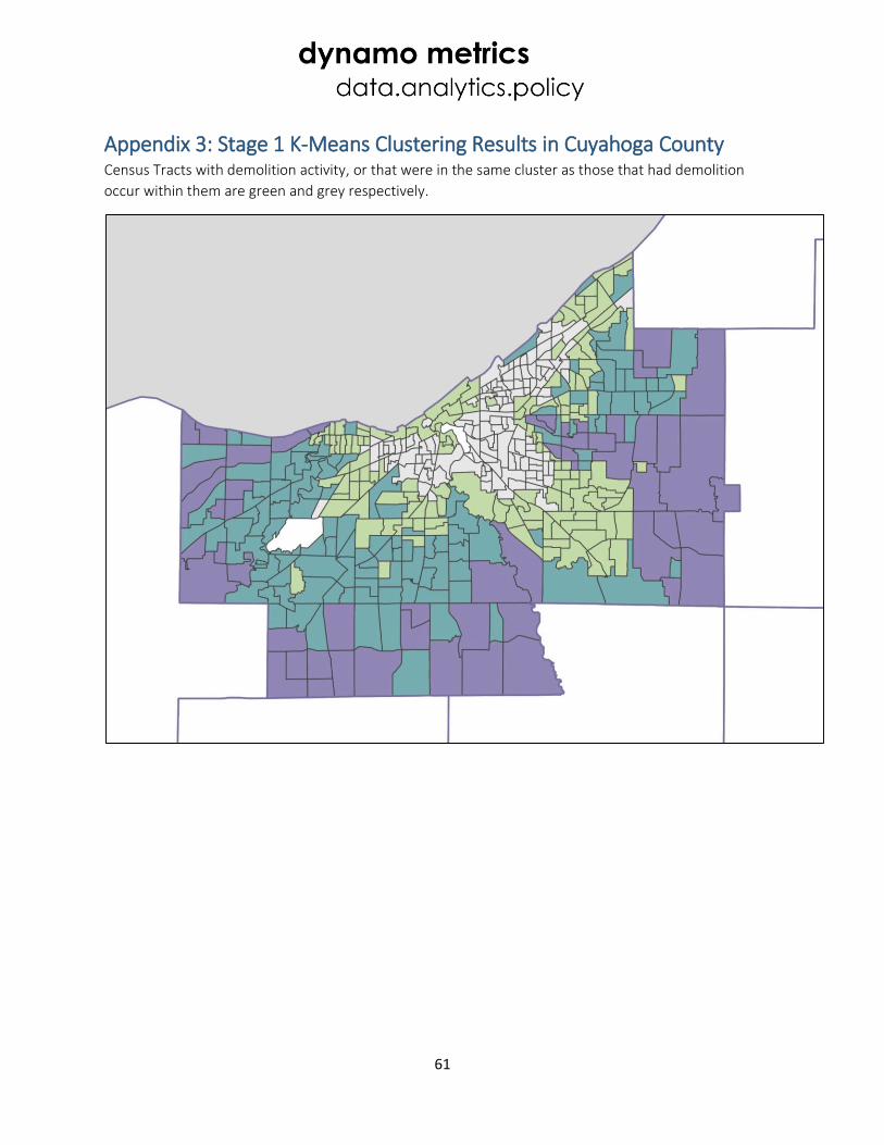
61
Appendix 3: Stage 1 K-Means Clustering Results in Cuyahoga County Census Tracts with demolition activity, or that were in the same cluster as those that had demolition
occur within them are green and grey respectively.
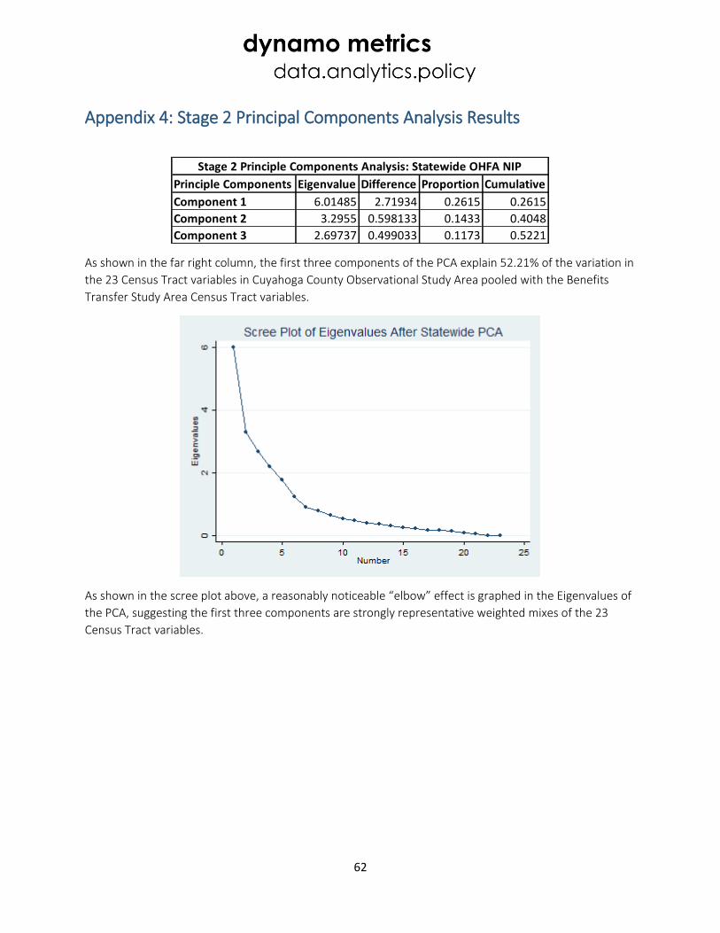
62
Appendix 4: Stage 2 Principal Components Analysis Results
As shown in the far right column, the first three components of the PCA explain 52.21% of the variation in
the 23 Census Tract variables in Cuyahoga County Observational Study Area pooled with the Benefits
Transfer Study Area Census Tract variables.
As shown in the scree plot above, a reasonably noticeable “elbow” effect is graphed in the Eigenvalues of
the PCA, suggesting the first three components are strongly representative weighted mixes of the 23
Census Tract variables.
Principle Components Eigenvalue Difference Proportion Cumulative
Component 1 6.01485 2.71934 0.2615 0.2615
Component 2 3.2955 0.598133 0.1433 0.4048
Component 3 2.69737 0.499033 0.1173 0.5221
Stage 2 Principle Components Analysis: Statewide OHFA NIP
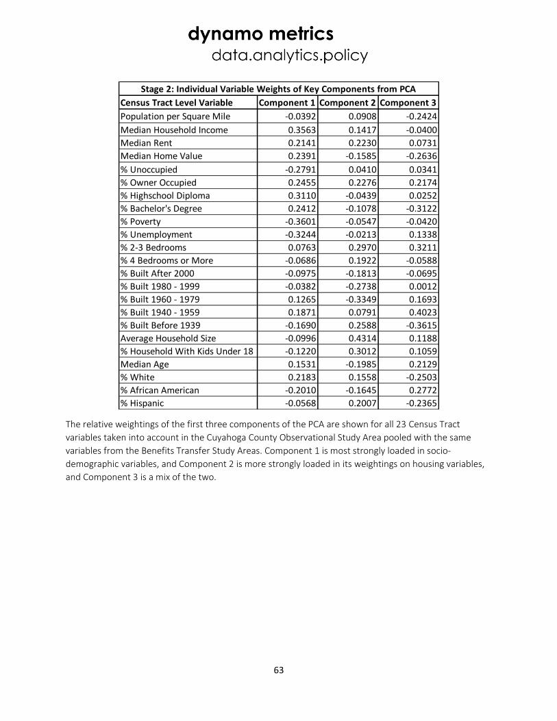
63
The relative weightings of the first three components of the PCA are shown for all 23 Census Tract
variables taken into account in the Cuyahoga County Observational Study Area pooled with the same
variables from the Benefits Transfer Study Areas. Component 1 is most strongly loaded in socio-
demographic variables, and Component 2 is more strongly loaded in its weightings on housing variables,
and Component 3 is a mix of the two.
Census Tract Level Variable Component 1 Component 2 Component 3
Population per Square Mile -0.0392 0.0908 -0.2424
Median Household Income 0.3563 0.1417 -0.0400
Median Rent 0.2141 0.2230 0.0731
Median Home Value 0.2391 -0.1585 -0.2636
% Unoccupied -0.2791 0.0410 0.0341
% Owner Occupied 0.2455 0.2276 0.2174
% Highschool Diploma 0.3110 -0.0439 0.0252
% Bachelor's Degree 0.2412 -0.1078 -0.3122
% Poverty -0.3601 -0.0547 -0.0420
% Unemployment -0.3244 -0.0213 0.1338
% 2-3 Bedrooms 0.0763 0.2970 0.3211
% 4 Bedrooms or More -0.0686 0.1922 -0.0588
% Built After 2000 -0.0975 -0.1813 -0.0695
% Built 1980 - 1999 -0.0382 -0.2738 0.0012
% Built 1960 - 1979 0.1265 -0.3349 0.1693
% Built 1940 - 1959 0.1871 0.0791 0.4023
% Built Before 1939 -0.1690 0.2588 -0.3615
Average Household Size -0.0996 0.4314 0.1188
% Household With Kids Under 18 -0.1220 0.3012 0.1059
Median Age 0.1531 -0.1985 0.2129
% White 0.2183 0.1558 -0.2503
% African American -0.2010 -0.1645 0.2772
% Hispanic -0.0568 0.2007 -0.2365
Stage 2: Individual Variable Weights of Key Components from PCA
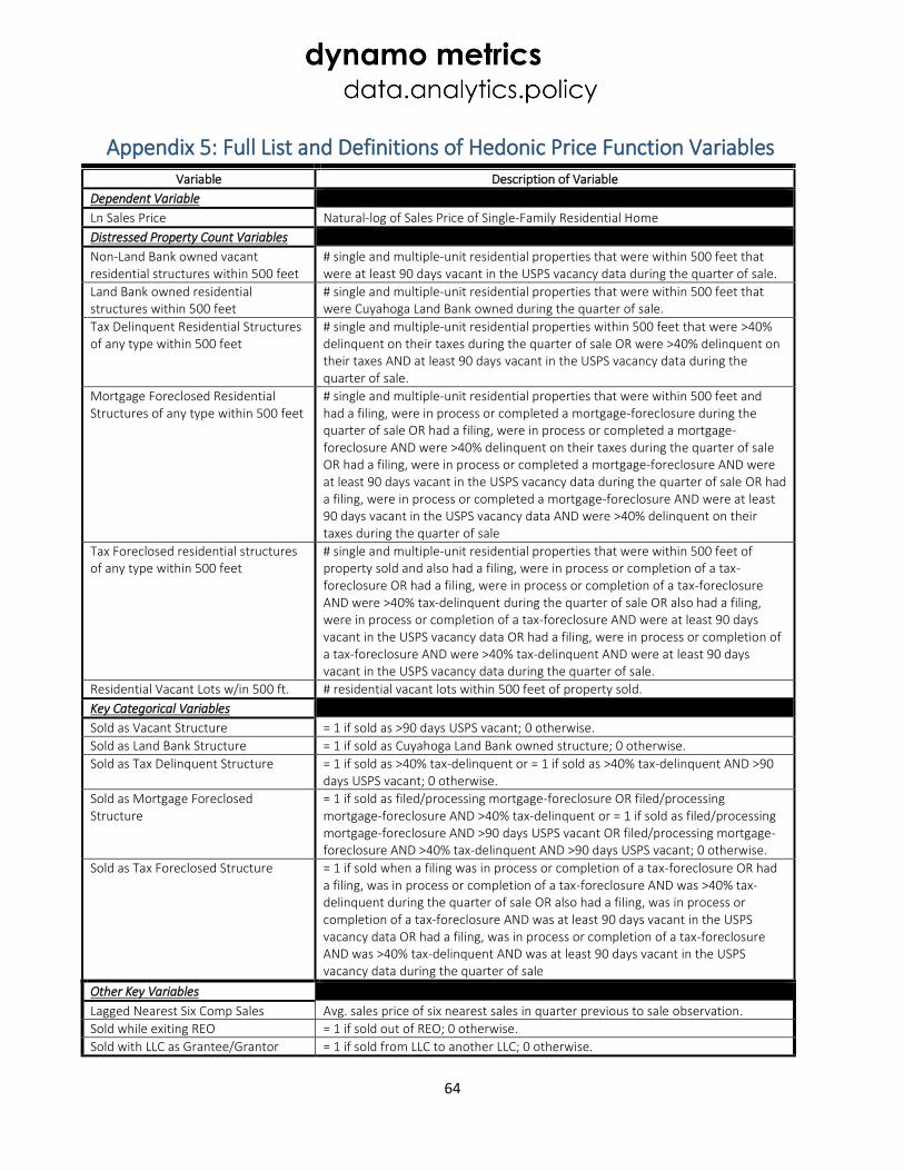
64
Appendix 5: Full List and Definitions of Hedonic Price Function Variables Variable Description of Variable
Dependent Variable
Ln Sales Price Natural-log of Sales Price of Single-Family Residential Home
Distressed Property Count Variables
Non-Land Bank owned vacant residential structures within 500 feet
# single and multiple-unit residential properties that were within 500 feet that were at least 90 days vacant in the USPS vacancy data during the quarter of sale.
Land Bank owned residential structures within 500 feet
# single and multiple-unit residential properties that were within 500 feet that were Cuyahoga Land Bank owned during the quarter of sale.
Tax Delinquent Residential Structures of any type within 500 feet
# single and multiple-unit residential properties within 500 feet that were >40% delinquent on their taxes during the quarter of sale OR were >40% delinquent on their taxes AND at least 90 days vacant in the USPS vacancy data during the quarter of sale.
Mortgage Foreclosed Residential Structures of any type within 500 feet
# single and multiple-unit residential properties that were within 500 feet and had a filing, were in process or completed a mortgage-foreclosure during the quarter of sale OR had a filing, were in process or completed a mortgage-foreclosure AND were >40% delinquent on their taxes during the quarter of sale OR had a filing, were in process or completed a mortgage-foreclosure AND were at least 90 days vacant in the USPS vacancy data during the quarter of sale OR had a filing, were in process or completed a mortgage-foreclosure AND were at least 90 days vacant in the USPS vacancy data AND were >40% delinquent on their taxes during the quarter of sale
Tax Foreclosed residential structures of any type within 500 feet
# single and multiple-unit residential properties that were within 500 feet of property sold and also had a filing, were in process or completion of a tax-foreclosure OR had a filing, were in process or completion of a tax-foreclosure AND were >40% tax-delinquent during the quarter of sale OR also had a filing, were in process or completion of a tax-foreclosure AND were at least 90 days vacant in the USPS vacancy data OR had a filing, were in process or completion of a tax-foreclosure AND were >40% tax-delinquent AND were at least 90 days vacant in the USPS vacancy data during the quarter of sale.
Residential Vacant Lots w/in 500 ft. # residential vacant lots within 500 feet of property sold.
Key Categorical Variables
Sold as Vacant Structure = 1 if sold as >90 days USPS vacant; 0 otherwise.
Sold as Land Bank Structure = 1 if sold as Cuyahoga Land Bank owned structure; 0 otherwise.
Sold as Tax Delinquent Structure = 1 if sold as >40% tax-delinquent or = 1 if sold as >40% tax-delinquent AND >90 days USPS vacant; 0 otherwise.
Sold as Mortgage Foreclosed Structure
= 1 if sold as filed/processing mortgage-foreclosure OR filed/processing mortgage-foreclosure AND >40% tax-delinquent or = 1 if sold as filed/processing mortgage-foreclosure AND >90 days USPS vacant OR filed/processing mortgage-foreclosure AND >40% tax-delinquent AND >90 days USPS vacant; 0 otherwise.
Sold as Tax Foreclosed Structure = 1 if sold when a filing was in process or completion of a tax-foreclosure OR had a filing, was in process or completion of a tax-foreclosure AND was >40% tax-delinquent during the quarter of sale OR also had a filing, was in process or completion of a tax-foreclosure AND was at least 90 days vacant in the USPS vacancy data OR had a filing, was in process or completion of a tax-foreclosure AND was >40% tax-delinquent AND was at least 90 days vacant in the USPS vacancy data during the quarter of sale
Other Key Variables
Lagged Nearest Six Comp Sales Avg. sales price of six nearest sales in quarter previous to sale observation.
Sold while exiting REO = 1 if sold out of REO; 0 otherwise.
Sold with LLC as Grantee/Grantor = 1 if sold from LLC to another LLC; 0 otherwise.
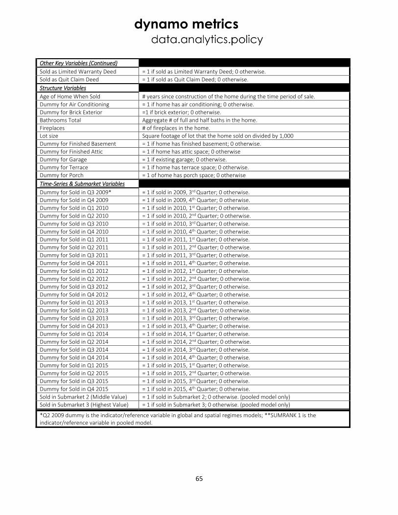
65
Other Key Variables (Continued)
Sold as Limited Warranty Deed = 1 if sold as Limited Warranty Deed; 0 otherwise.
Sold as Quit Claim Deed = 1 if sold as Quit Claim Deed; 0 otherwise.
Structure Variables
Age of Home When Sold # years since construction of the home during the time period of sale.
Dummy for Air Conditioning = 1 if home has air conditioning; 0 otherwise.
Dummy for Brick Exterior =1 if brick exterior; 0 otherwise.
Bathrooms Total Aggregate # of full and half baths in the home.
Fireplaces # of fireplaces in the home.
Lot size Square footage of lot that the home sold on divided by 1,000
Dummy for Finished Basement = 1 if home has finished basement; 0 otherwise.
Dummy for Finished Attic = 1 if home has attic space; 0 otherwise
Dummy for Garage = 1 if existing garage; 0 otherwise.
Dummy for Terrace = 1 if home has terrace space; 0 otherwise.
Dummy for Porch = 1 of home has porch space; 0 otherwise
Time-Series & Submarket Variables
Dummy for Sold in Q3 2009* = 1 if sold in 2009, 3rd Quarter; 0 otherwise.
Dummy for Sold in Q4 2009 = 1 if sold in 2009, 4th Quarter; 0 otherwise.
Dummy for Sold in Q1 2010 = 1 if sold in 2010, 1st Quarter; 0 otherwise.
Dummy for Sold in Q2 2010 = 1 if sold in 2010, 2nd Quarter; 0 otherwise.
Dummy for Sold in Q3 2010 = 1 if sold in 2010, 3rd Quarter; 0 otherwise.
Dummy for Sold in Q4 2010 = 1 if sold in 2010, 4th Quarter; 0 otherwise.
Dummy for Sold in Q1 2011 = 1 if sold in 2011, 1st Quarter; 0 otherwise.
Dummy for Sold in Q2 2011 = 1 if sold in 2011, 2nd Quarter; 0 otherwise.
Dummy for Sold in Q3 2011 = 1 if sold in 2011, 3rd Quarter; 0 otherwise.
Dummy for Sold in Q4 2011 = 1 if sold in 2011, 4th Quarter; 0 otherwise.
Dummy for Sold in Q1 2012 = 1 if sold in 2012, 1st Quarter; 0 otherwise.
Dummy for Sold in Q2 2012 = 1 if sold in 2012, 2nd Quarter; 0 otherwise.
Dummy for Sold in Q3 2012 = 1 if sold in 2012, 3rd Quarter; 0 otherwise.
Dummy for Sold in Q4 2012 = 1 if sold in 2012, 4th Quarter; 0 otherwise.
Dummy for Sold in Q1 2013 = 1 if sold in 2013, 1st Quarter; 0 otherwise.
Dummy for Sold in Q2 2013 = 1 if sold in 2013, 2nd Quarter; 0 otherwise.
Dummy for Sold in Q3 2013 = 1 if sold in 2013, 3rd Quarter; 0 otherwise.
Dummy for Sold in Q4 2013 = 1 if sold in 2013, 4th Quarter; 0 otherwise.
Dummy for Sold in Q1 2014 = 1 if sold in 2014, 1st Quarter; 0 otherwise.
Dummy for Sold in Q2 2014 = 1 if sold in 2014, 2nd Quarter; 0 otherwise.
Dummy for Sold in Q3 2014 = 1 if sold in 2014, 3rd Quarter; 0 otherwise.
Dummy for Sold in Q4 2014 = 1 if sold in 2014, 4th Quarter; 0 otherwise.
Dummy for Sold in Q1 2015 = 1 if sold in 2015, 1st Quarter; 0 otherwise.
Dummy for Sold in Q2 2015 = 1 if sold in 2015, 2nd Quarter; 0 otherwise.
Dummy for Sold in Q3 2015 = 1 if sold in 2015, 3rd Quarter; 0 otherwise.
Dummy for Sold in Q4 2015 = 1 if sold in 2015, 4th Quarter; 0 otherwise.
Sold in Submarket 2 (Middle Value) = 1 if sold in Submarket 2; 0 otherwise. (pooled model only)
Sold in Submarket 3 (Highest Value) = 1 if sold in Submarket 3; 0 otherwise. (pooled model only)
*Q2 2009 dummy is the indicator/reference variable in global and spatial regimes models; **SUMRANK 1 is the indicator/reference variable in pooled model.
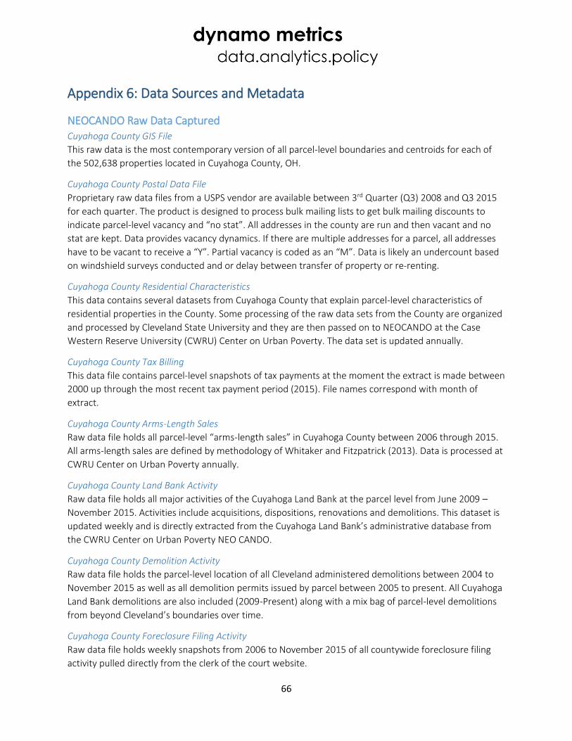
66
Appendix 6: Data Sources and Metadata
NEOCANDO Raw Data Captured Cuyahoga County GIS File
This raw data is the most contemporary version of all parcel-level boundaries and centroids for each of
the 502,638 properties located in Cuyahoga County, OH.
Cuyahoga County Postal Data File
Proprietary raw data files from a USPS vendor are available between 3rd Quarter (Q3) 2008 and Q3 2015
for each quarter. The product is designed to process bulk mailing lists to get bulk mailing discounts to
indicate parcel-level vacancy and “no stat”. All addresses in the county are run and then vacant and no
stat are kept. Data provides vacancy dynamics. If there are multiple addresses for a parcel, all addresses
have to be vacant to receive a “Y”. Partial vacancy is coded as an “M”. Data is likely an undercount based
on windshield surveys conducted and or delay between transfer of property or re-renting.
Cuyahoga County Residential Characteristics
This data contains several datasets from Cuyahoga County that explain parcel-level characteristics of
residential properties in the County. Some processing of the raw data sets from the County are organized
and processed by Cleveland State University and they are then passed on to NEOCANDO at the Case
Western Reserve University (CWRU) Center on Urban Poverty. The data set is updated annually.
Cuyahoga County Tax Billing
This data file contains parcel-level snapshots of tax payments at the moment the extract is made between
2000 up through the most recent tax payment period (2015). File names correspond with month of
extract.
Cuyahoga County Arms-Length Sales
Raw data file holds all parcel-level “arms-length sales” in Cuyahoga County between 2006 through 2015.
All arms-length sales are defined by methodology of Whitaker and Fitzpatrick (2013). Data is processed at
CWRU Center on Urban Poverty annually.
Cuyahoga County Land Bank Activity
Raw data file holds all major activities of the Cuyahoga Land Bank at the parcel level from June 2009 –
November 2015. Activities include acquisitions, dispositions, renovations and demolitions. This dataset is
updated weekly and is directly extracted from the Cuyahoga Land Bank’s administrative database from
the CWRU Center on Urban Poverty NEO CANDO.
Cuyahoga County Demolition Activity
Raw data file holds the parcel-level location of all Cleveland administered demolitions between 2004 to
November 2015 as well as all demolition permits issued by parcel between 2005 to present. All Cuyahoga
Land Bank demolitions are also included (2009-Present) along with a mix bag of parcel-level demolitions
from beyond Cleveland’s boundaries over time.
Cuyahoga County Foreclosure Filing Activity
Raw data file holds weekly snapshots from 2006 to November 2015 of all countywide foreclosure filing
activity pulled directly from the clerk of the court website.
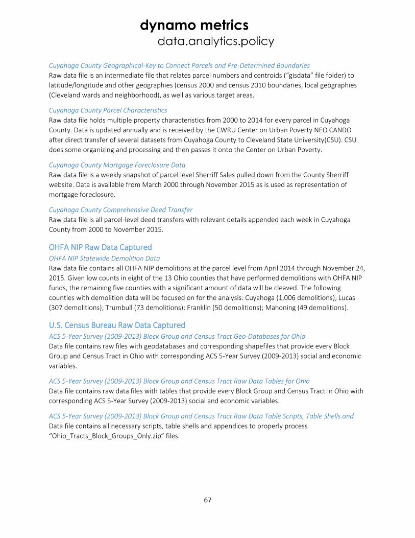
67
Cuyahoga County Geographical-Key to Connect Parcels and Pre-Determined Boundaries
Raw data file is an intermediate file that relates parcel numbers and centroids (“gisdata” file folder) to
latitude/longitude and other geographies (census 2000 and census 2010 boundaries, local geographies
(Cleveland wards and neighborhood), as well as various target areas.
Cuyahoga County Parcel Characteristics
Raw data file holds multiple property characteristics from 2000 to 2014 for every parcel in Cuyahoga
County. Data is updated annually and is received by the CWRU Center on Urban Poverty NEO CANDO
after direct transfer of several datasets from Cuyahoga County to Cleveland State University(CSU). CSU
does some organizing and processing and then passes it onto the Center on Urban Poverty.
Cuyahoga County Mortgage Foreclosure Data
Raw data file is a weekly snapshot of parcel level Sherriff Sales pulled down from the County Sherriff
website. Data is available from March 2000 through November 2015 as is used as representation of
mortgage foreclosure.
Cuyahoga County Comprehensive Deed Transfer
Raw data file is all parcel-level deed transfers with relevant details appended each week in Cuyahoga
County from 2000 to November 2015.
OHFA NIP Raw Data Captured OHFA NIP Statewide Demolition Data
Raw data file contains all OHFA NIP demolitions at the parcel level from April 2014 through November 24,
2015. Given low counts in eight of the 13 Ohio counties that have performed demolitions with OHFA NIP
funds, the remaining five counties with a significant amount of data will be cleaved. The following
counties with demolition data will be focused on for the analysis: Cuyahoga (1,006 demolitions); Lucas
(307 demolitions); Trumbull (73 demolitions); Franklin (50 demolitions); Mahoning (49 demolitions).
U.S. Census Bureau Raw Data Captured ACS 5-Year Survey (2009-2013) Block Group and Census Tract Geo-Databases for Ohio
Data file contains raw files with geodatabases and corresponding shapefiles that provide every Block
Group and Census Tract in Ohio with corresponding ACS 5-Year Survey (2009-2013) social and economic
variables.
ACS 5-Year Survey (2009-2013) Block Group and Census Tract Raw Data Tables for Ohio
Data file contains raw data files with tables that provide every Block Group and Census Tract in Ohio with
corresponding ACS 5-Year Survey (2009-2013) social and economic variables.
ACS 5-Year Survey (2009-2013) Block Group and Census Tract Raw Data Table Scripts, Table Shells and
Data file contains all necessary scripts, table shells and appendices to properly process
“Ohio_Tracts_Block_Groups_Only.zip” files.
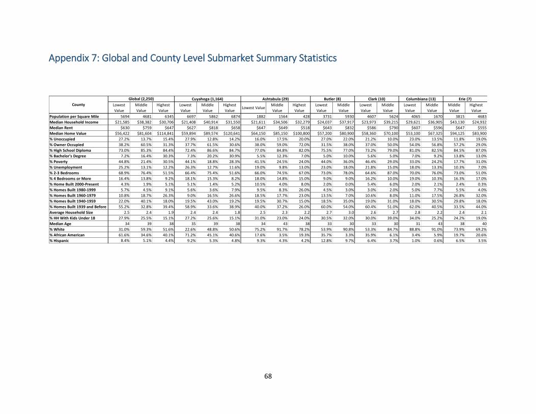
68
Appendix 7: Global and County Level Submarket Summary Statistics
Lowest
Value
Middle
Value
Highest
Value
Lowest
Value
Middle
Value
Highest
ValueLowest Value
Middle
Value
Highest
Value
Lowest
Value
Middle
Value
Lowest
Value
Middle
Value
Lowest
Value
Middle
Value
Middle
Value
Highest
Value
Population per Square Mile 5694 4681 6345 6697 5862 6874 1882 1564 428 3731 5930 4607 5624 4065 1670 3815 4683
Median Household Income $21,585 $38,382 $30,706 $21,408 $40,914 $31,550 $21,611 $34,506 $32,279 $24,037 $37,917 $23,973 $39,215 $29,621 $36,905 $43,130 $24,932
Median Rent $630 $759 $647 $627 $818 $658 $647 $649 $518 $643 $832 $586 $790 $607 $596 $647 $555
Median Home Value $56,422 $81,604 $114,841 $59,894 $89,574 $120,641 $64,150 $85,150 $100,800 $57,200 $80,900 $58,360 $70,100 $53,100 $67,325 $94,125 $83,900
% Unoccupied 27.2% 13.7% 15.4% 27.9% 12.8% 14.2% 16.0% 17.5% 20.0% 27.0% 22.0% 21.2% 10.0% 23.0% 13.5% 11.8% 19.0%
% Owner Occupied 38.2% 60.5% 31.3% 37.7% 61.5% 30.6% 38.0% 59.0% 72.0% 31.5% 38.0% 37.0% 50.0% 54.0% 56.8% 57.2% 29.0%
% High School Diploma 73.0% 85.3% 84.4% 72.4% 86.6% 84.7% 77.0% 84.8% 82.0% 75.5% 77.0% 73.2% 79.0% 81.0% 82.5% 84.5% 87.0%
% Bachelor's Degree 7.2% 16.4% 30.3% 7.3% 20.2% 30.9% 5.5% 12.3% 7.0% 5.0% 10.0% 5.6% 5.0% 7.0% 9.2% 13.8% 13.0%
% Poverty 44.8% 21.4% 30.5% 44.1% 18.8% 28.3% 41.5% 24.5% 24.0% 44.0% 36.0% 46.4% 29.0% 33.0% 24.2% 17.7% 31.0%
% Unemployment 25.2% 13.1% 12.2% 26.3% 12.7% 11.6% 19.0% 9.8% 13.0% 23.0% 18.0% 21.8% 15.0% 18.0% 13.3% 10.3% 7.0%
% 2-3 Bedrooms 68.9% 76.4% 51.5% 66.4% 75.4% 51.6% 66.0% 74.5% 67.0% 73.0% 78.0% 64.6% 87.0% 70.0% 76.0% 73.0% 51.0%
% 4 Bedrooms or More 16.4% 13.8% 9.2% 18.1% 15.3% 8.2% 18.0% 14.8% 15.0% 9.0% 9.0% 16.2% 10.0% 19.0% 10.3% 16.3% 17.0%
% Home Built 2000-Present 4.3% 1.9% 5.1% 5.1% 1.4% 5.2% 10.5% 4.0% 8.0% 2.0% 0.0% 5.4% 6.0% 2.0% 2.1% 2.4% 0.3%
% Homes Built 1980-1999 5.7% 4.5% 9.1% 5.6% 3.6% 7.9% 9.5% 8.3% 26.0% 4.5% 3.0% 3.0% 2.0% 5.0% 7.7% 5.5% 4.0%
% Homes Built 1960-1979 10.8% 18.7% 26.3% 9.0% 16.5% 26.6% 18.5% 17.7% 23.0% 13.5% 7.0% 10.6% 8.0% 11.0% 17.5% 26.8% 32.0%
% Homes Built 1940-1959 22.0% 40.1% 18.0% 19.5% 43.0% 19.2% 19.5% 30.7% 15.0% 18.5% 35.0% 19.0% 31.0% 18.0% 30.5% 29.8% 18.0%
% Homes Built 1939 and Before 55.2% 32.8% 39.4% 58.9% 33.6% 38.9% 40.0% 37.2% 26.0% 60.0% 54.0% 60.4% 51.0% 62.0% 40.5% 33.5% 44.0%
Average Household Size 2.5 2.4 1.9 2.4 2.4 1.8 2.5 2.3 2.2 2.7 3.0 2.6 2.7 2.8 2.2 2.4 2.1
% HH With Kids Under 18 27.9% 25.5% 15.1% 27.2% 25.6% 15.1% 31.0% 23.0% 24.0% 30.5% 32.0% 30.0% 39.0% 34.0% 25.2% 24.2% 19.0%
Median Age 34 39 38 35 39 38 34 43 38 33 30 33 30 31 43 38 40
% White 31.0% 59.3% 51.6% 22.6% 48.8% 50.6% 75.2% 91.7% 78.2% 53.9% 90.8% 53.3% 84.7% 88.8% 91.0% 73.9% 69.2%
% African American 61.6% 34.6% 40.1% 71.2% 45.1% 40.6% 17.6% 3.5% 19.3% 35.7% 3.3% 35.9% 6.1% 3.4% 5.9% 19.7% 20.6%
% Hispanic 8.4% 5.1% 4.4% 9.2% 5.3% 4.8% 9.3% 4.3% 4.2% 12.8% 9.7% 6.4% 3.7% 1.0% 0.6% 6.5% 3.5%
County
Global (2,250) Cuyahoga (1,164) Ashtabula (29) Butler (8) Clark (10) Columbiana (13) Erie (7)
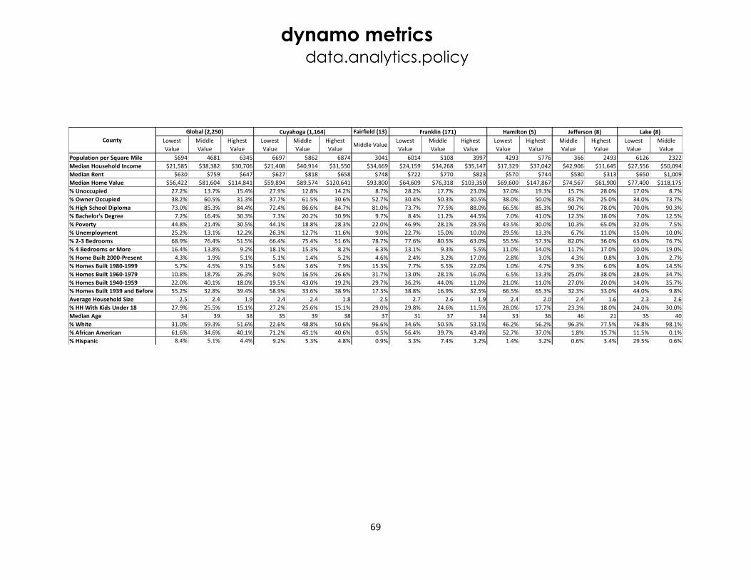
69
Fairfield (13)
Lowest
Value
Middle
Value
Highest
Value
Lowest
Value
Middle
Value
Highest
ValueMiddle Value
Lowest
Value
Middle
Value
Highest
Value
Lowest
Value
Highest
Value
Middle
Value
Highest
Value
Lowest
Value
Middle
Value
Population per Square Mile 5694 4681 6345 6697 5862 6874 3041 6014 5108 3997 4293 5776 366 2493 6126 2322
Median Household Income $21,585 $38,382 $30,706 $21,408 $40,914 $31,550 $34,669 $24,159 $34,268 $35,147 $17,329 $37,042 $42,906 $11,645 $27,556 $50,094
Median Rent $630 $759 $647 $627 $818 $658 $748 $722 $770 $823 $570 $744 $580 $313 $650 $1,009
Median Home Value $56,422 $81,604 $114,841 $59,894 $89,574 $120,641 $93,800 $64,609 $76,318 $103,350 $69,600 $147,867 $74,567 $61,900 $77,400 $118,175
% Unoccupied 27.2% 13.7% 15.4% 27.9% 12.8% 14.2% 8.7% 28.2% 17.7% 23.0% 37.0% 19.3% 15.7% 28.0% 17.0% 8.7%
% Owner Occupied 38.2% 60.5% 31.3% 37.7% 61.5% 30.6% 52.7% 30.4% 50.3% 30.5% 38.0% 50.0% 83.7% 25.0% 34.0% 73.7%
% High School Diploma 73.0% 85.3% 84.4% 72.4% 86.6% 84.7% 81.0% 73.7% 77.5% 88.0% 66.5% 85.3% 90.7% 78.0% 70.0% 90.3%
% Bachelor's Degree 7.2% 16.4% 30.3% 7.3% 20.2% 30.9% 9.7% 8.4% 11.2% 44.5% 7.0% 41.0% 12.3% 18.0% 7.0% 12.5%
% Poverty 44.8% 21.4% 30.5% 44.1% 18.8% 28.3% 22.0% 46.9% 28.1% 28.5% 43.5% 30.0% 10.3% 65.0% 32.0% 7.5%
% Unemployment 25.2% 13.1% 12.2% 26.3% 12.7% 11.6% 9.0% 22.7% 15.0% 10.0% 29.5% 13.3% 6.7% 11.0% 15.0% 10.0%
% 2-3 Bedrooms 68.9% 76.4% 51.5% 66.4% 75.4% 51.6% 78.7% 77.6% 80.5% 63.0% 55.5% 57.3% 82.0% 36.0% 63.0% 76.7%
% 4 Bedrooms or More 16.4% 13.8% 9.2% 18.1% 15.3% 8.2% 6.3% 13.1% 9.3% 5.5% 11.0% 14.0% 11.7% 17.0% 10.0% 19.0%
% Home Built 2000-Present 4.3% 1.9% 5.1% 5.1% 1.4% 5.2% 4.6% 2.4% 3.2% 17.0% 2.8% 3.0% 4.3% 0.8% 3.0% 2.7%
% Homes Built 1980-1999 5.7% 4.5% 9.1% 5.6% 3.6% 7.9% 15.3% 7.7% 5.5% 22.0% 1.0% 4.7% 9.3% 6.0% 8.0% 14.5%
% Homes Built 1960-1979 10.8% 18.7% 26.3% 9.0% 16.5% 26.6% 31.7% 13.0% 28.1% 16.0% 6.5% 13.3% 25.0% 38.0% 28.0% 34.7%
% Homes Built 1940-1959 22.0% 40.1% 18.0% 19.5% 43.0% 19.2% 29.7% 36.2% 44.0% 11.0% 21.0% 11.0% 27.0% 20.0% 14.0% 35.7%
% Homes Built 1939 and Before 55.2% 32.8% 39.4% 58.9% 33.6% 38.9% 17.3% 38.8% 16.9% 32.5% 66.5% 65.3% 32.3% 33.0% 44.0% 9.8%
Average Household Size 2.5 2.4 1.9 2.4 2.4 1.8 2.5 2.7 2.6 1.9 2.4 2.0 2.4 1.6 2.3 2.6
% HH With Kids Under 18 27.9% 25.5% 15.1% 27.2% 25.6% 15.1% 29.0% 29.8% 24.6% 11.5% 28.0% 17.7% 23.3% 18.0% 24.0% 30.0%
Median Age 34 39 38 35 39 38 37 31 37 34 33 36 46 21 35 40
% White 31.0% 59.3% 51.6% 22.6% 48.8% 50.6% 96.6% 34.6% 50.5% 53.1% 46.2% 56.2% 96.3% 77.5% 76.8% 98.1%
% African American 61.6% 34.6% 40.1% 71.2% 45.1% 40.6% 0.5% 56.4% 39.7% 43.4% 52.7% 37.0% 1.8% 15.7% 11.5% 0.1%
% Hispanic 8.4% 5.1% 4.4% 9.2% 5.3% 4.8% 0.9% 3.3% 7.4% 3.2% 1.4% 3.2% 0.6% 3.4% 29.5% 0.6%
Lake (8)
County
Global (2,250) Cuyahoga (1,164) Franklin (171) Hamilton (5) Jefferson (8)
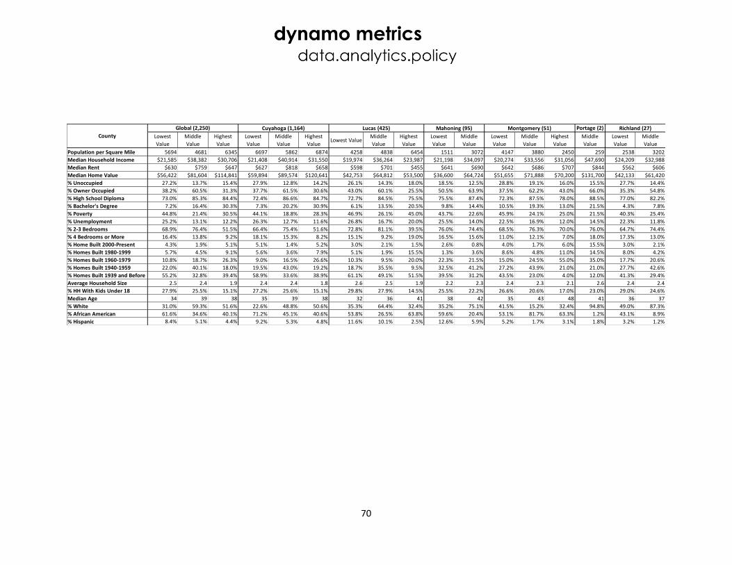
70
Portage (2)
Lowest
Value
Middle
Value
Highest
Value
Lowest
Value
Middle
Value
Highest
ValueLowest Value
Middle
Value
Highest
Value
Lowest
Value
Middle
Value
Lowest
Value
Middle
Value
Highest
Value
Middle
Value
Lowest
Value
Middle
Value
Population per Square Mile 5694 4681 6345 6697 5862 6874 4258 4838 6454 1511 3072 4147 3880 2450 259 2538 3202
Median Household Income $21,585 $38,382 $30,706 $21,408 $40,914 $31,550 $19,974 $36,264 $23,987 $21,198 $34,097 $20,274 $33,556 $31,056 $47,690 $24,209 $32,988
Median Rent $630 $759 $647 $627 $818 $658 $598 $701 $455 $641 $690 $642 $686 $707 $844 $562 $606
Median Home Value $56,422 $81,604 $114,841 $59,894 $89,574 $120,641 $42,753 $64,812 $53,500 $36,600 $64,724 $51,655 $71,888 $70,200 $131,700 $42,133 $61,420
% Unoccupied 27.2% 13.7% 15.4% 27.9% 12.8% 14.2% 26.1% 14.3% 18.0% 18.5% 12.5% 28.8% 19.1% 16.0% 15.5% 27.7% 14.4%
% Owner Occupied 38.2% 60.5% 31.3% 37.7% 61.5% 30.6% 43.0% 60.1% 25.5% 50.5% 63.9% 37.5% 62.2% 43.0% 66.0% 35.3% 54.8%
% High School Diploma 73.0% 85.3% 84.4% 72.4% 86.6% 84.7% 72.7% 84.5% 75.5% 75.5% 87.4% 72.3% 87.5% 78.0% 88.5% 77.0% 82.2%
% Bachelor's Degree 7.2% 16.4% 30.3% 7.3% 20.2% 30.9% 6.1% 13.5% 20.5% 9.8% 14.4% 10.5% 19.3% 13.0% 21.5% 4.3% 7.8%
% Poverty 44.8% 21.4% 30.5% 44.1% 18.8% 28.3% 46.9% 26.1% 45.0% 43.7% 22.6% 45.9% 24.1% 25.0% 21.5% 40.3% 25.4%
% Unemployment 25.2% 13.1% 12.2% 26.3% 12.7% 11.6% 26.8% 16.7% 20.0% 25.5% 14.0% 22.5% 16.9% 12.0% 14.5% 22.3% 11.8%
% 2-3 Bedrooms 68.9% 76.4% 51.5% 66.4% 75.4% 51.6% 72.8% 81.1% 39.5% 76.0% 74.4% 68.5% 76.3% 70.0% 76.0% 64.7% 74.4%
% 4 Bedrooms or More 16.4% 13.8% 9.2% 18.1% 15.3% 8.2% 15.1% 9.2% 19.0% 16.5% 15.6% 11.0% 12.1% 7.0% 18.0% 17.3% 13.0%
% Home Built 2000-Present 4.3% 1.9% 5.1% 5.1% 1.4% 5.2% 3.0% 2.1% 1.5% 2.6% 0.8% 4.0% 1.7% 6.0% 15.5% 3.0% 2.1%
% Homes Built 1980-1999 5.7% 4.5% 9.1% 5.6% 3.6% 7.9% 5.1% 1.9% 15.5% 1.3% 3.6% 8.6% 4.8% 11.0% 14.5% 8.0% 4.2%
% Homes Built 1960-1979 10.8% 18.7% 26.3% 9.0% 16.5% 26.6% 10.3% 9.5% 20.0% 22.3% 21.5% 15.0% 24.5% 55.0% 35.0% 17.7% 20.6%
% Homes Built 1940-1959 22.0% 40.1% 18.0% 19.5% 43.0% 19.2% 18.7% 35.5% 9.5% 32.5% 41.2% 27.2% 43.9% 21.0% 21.0% 27.7% 42.6%
% Homes Built 1939 and Before 55.2% 32.8% 39.4% 58.9% 33.6% 38.9% 61.1% 49.1% 51.5% 39.5% 31.2% 43.5% 23.0% 4.0% 12.0% 41.3% 29.4%
Average Household Size 2.5 2.4 1.9 2.4 2.4 1.8 2.6 2.5 1.9 2.2 2.3 2.4 2.3 2.1 2.6 2.4 2.4
% HH With Kids Under 18 27.9% 25.5% 15.1% 27.2% 25.6% 15.1% 29.8% 27.9% 14.5% 25.5% 22.2% 26.6% 20.6% 17.0% 23.0% 29.0% 24.6%
Median Age 34 39 38 35 39 38 32 36 41 38 42 35 43 48 41 36 37
% White 31.0% 59.3% 51.6% 22.6% 48.8% 50.6% 35.3% 64.4% 32.4% 35.2% 75.1% 41.5% 15.2% 32.4% 94.8% 49.0% 87.3%
% African American 61.6% 34.6% 40.1% 71.2% 45.1% 40.6% 53.8% 26.5% 63.8% 59.6% 20.4% 53.1% 81.7% 63.3% 1.2% 43.1% 8.9%
% Hispanic 8.4% 5.1% 4.4% 9.2% 5.3% 4.8% 11.6% 10.1% 2.5% 12.6% 5.9% 5.2% 1.7% 3.1% 1.8% 3.2% 1.2%
County
Global (2,250) Cuyahoga (1,164) Lucas (425) Mahoning (95) Montgomery (51) Richland (27)

71
Lowest
Value
Middle
Value
Highest
Value
Lowest
Value
Middle
Value
Highest
ValueLowest Value
Middle
Value
Highest
Value
Lowest
Value
Middle
Value
Highest
Value
Lowest
Value
Middle
Value
Population per Square Mile 5694 4681 6345 6697 5862 6874 4211 3737 2650 4523 4474 4562 2695 3106
Median Household Income $21,585 $38,382 $30,706 $21,408 $40,914 $31,550 $23,530 $28,455 $10,871 $23,110 $33,968 $15,970 $17,500 $30,811
Median Rent $630 $759 $647 $627 $818 $658 $586 $627 $288 $798 $636 $707 $520 $638
Median Home Value $56,422 $81,604 $114,841 $59,894 $89,574 $120,641 $51,333 $62,967 $75,700 $64,100 $66,800 $47,300 $39,567 $57,883
% Unoccupied 27.2% 13.7% 15.4% 27.9% 12.8% 14.2% 25.2% 11.3% 19.0% 29.0% 18.5% 22.0% 29.0% 15.5%
% Owner Occupied 38.2% 60.5% 31.3% 37.7% 61.5% 30.6% 46.5% 52.7% 11.0% 40.5% 54.5% 2.0% 41.3% 54.2%
% High School Diploma 73.0% 85.3% 84.4% 72.4% 86.6% 84.7% 76.5% 79.3% 80.0% 83.0% 77.0% 98.0% 75.7% 81.8%
% Bachelor's Degree 7.2% 16.4% 30.3% 7.3% 20.2% 30.9% 5.2% 5.3% 2.0% 4.0% 11.5% 52.0% 3.7% 7.7%
% Poverty 44.8% 21.4% 30.5% 44.1% 18.8% 28.3% 45.0% 30.7% 59.0% 37.5% 28.5% 65.0% 52.3% 29.3%
% Unemployment 25.2% 13.1% 12.2% 26.3% 12.7% 11.6% 19.8% 16.0% 29.0% 29.0% 10.5% 14.0% 16.7% 8.2%
% 2-3 Bedrooms 68.9% 76.4% 51.5% 66.4% 75.4% 51.6% 70.5% 79.3% 7.0% 80.5% 75.5% 52.0% 65.3% 77.0%
% 4 Bedrooms or More 16.4% 13.8% 9.2% 18.1% 15.3% 8.2% 14.8% 10.0% 6.0% 16.0% 14.5% 13.0% 15.0% 12.0%
% Home Built 2000-Present 4.3% 1.9% 5.1% 5.1% 1.4% 5.2% 4.3% 2.3% 2.0% 4.0% 0.9% 2.0% 3.0% 1.2%
% Homes Built 1980-1999 5.7% 4.5% 9.1% 5.6% 3.6% 7.9% 5.7% 3.2% 10.0% 2.0% 6.0% 30.0% 6.7% 4.2%
% Homes Built 1960-1979 10.8% 18.7% 26.3% 9.0% 16.5% 26.6% 14.7% 15.3% 30.0% 7.0% 15.0% 32.0% 22.3% 23.2%
% Homes Built 1940-1959 22.0% 40.1% 18.0% 19.5% 43.0% 19.2% 20.7% 34.7% 17.0% 28.5% 38.5% 8.0% 29.0% 39.2%
% Homes Built 1939 and Before 55.2% 32.8% 39.4% 58.9% 33.6% 38.9% 52.3% 42.7% 39.0% 56.0% 37.5% 26.0% 37.0% 30.0%
Average Household Size 2.5 2.4 1.9 2.4 2.4 1.8 2.5 2.4 1.2 2.5 2.5 2.6 2.3 2.4
% HH With Kids Under 18 27.9% 25.5% 15.1% 27.2% 25.6% 15.1% 27.3% 28.7% 4.0% 22.0% 34.5% 9.0% 26.3% 26.7%
Median Age 34 39 38 35 39 38 33 36 55 37 31 21 34 37
% White 31.0% 59.3% 51.6% 22.6% 48.8% 50.6% 55.8% 69.9% 58.2% 42.6% 56.6% 65.2% 56.2% 69.9%
% African American 61.6% 34.6% 40.1% 71.2% 45.1% 40.6% 33.8% 21.5% 34.7% 51.4% 27.9% 17.3% 38.2% 25.0%
% Hispanic 8.4% 5.1% 4.4% 9.2% 5.3% 4.8% 2.3% 3.1% 1.1% 1.6% 2.2% 2.1% 2.7% 2.0%
County
Global (2,250) Cuyahoga (1,164) Stark (87) Summit (16) Trumbull (111)

72
Appendix 8: Global and Three-Submarket Regime Hedonic Model Results

73
Appendix 9: Three-Submarket Regime Hedonic Model Chow Test Results

74
Appendix 10: OHFA NIP Benefit-Cost Ratio by County Submarket 71
County SubmarketOHFA NIP
Demolitions
Estimated
Housing Units
Within 500
Total
Demolition Cost
OHFA NIP Demolition Impact
by Submarket
County
Submarket
BCR
Lowest Value 14 29 $218,836 $389,051 1.78
Middle Value 14 76 $210,234 $1,142,102 5.43
Highest Value 1 0 $12,549 $0 0.00
Lowest Value 6 68 $75,294 $404,149 5.37
Middle Value 2 24 $25,098 $213,421 8.50
Lowest Value 9 97 $132,401 $331,363 2.50
Middle Value 1 30 $14,448 $115,581 8.00
Lowest Value 5 29 $62,745 $242,688 3.87
Middle Value 8 97 $147,231 $648,616 4.41
Lowest Value 990 3870 $12,492,387 $54,812,066 4.39
Middle Value 138 1068 $1,671,274 $14,403,076 8.62
Highest Value 34 440 $409,267 $1,802,059 4.40
Middle Value 5 66 $66,877 $426,600 6.38
Highest Value 2 25 $47,611 $78,849 1.66
Fairfield Middle Value 13 36 $201,988 $843,114 4.17
Lowest Value 145 639 $2,340,103 $8,455,530 3.61
Middle Value 22 233 $335,554 $2,153,547 6.42
Highest Value 4 55 $60,172 $215,874 3.59
Lowest Value 2 38 $37,549 $84,121 2.24
Highest Value 3 60 $37,647 $158,046 4.20
Middle Value 6 15 $84,837 $103,028 1.21
Highest Value 2 59 $25,098 $137,290 5.47
Lowest Value 2 7 $23,030 $34,155 1.48
Middle Value 6 40 $100,273 $377,388 3.76
Lowest Value 330 830 $3,248,720 $10,725,998 3.30
Middle Value 86 452 $838,227 $7,279,128 8.68
Highest Value 9 31 $110,544 $228,597 2.07
Lowest Value 13 49 $169,873 $238,827 1.41
Middle Value 82 218 $1,231,106 $3,562,018 2.89
Lowest Value 30 222 $399,192 $1,050,634 2.63
Middle Value 20 179 $283,757 $1,937,214 6.83
Highest Value 1 17 $13,586 $22,431 1.65
Portage Middle Value 2 12 $19,844 $75,284 3.79
Lowest Value 15 28 $170,081 $180,307 1.06
Middle Value 12 68 $159,066 $507,143 3.19
Lowest Value 80 110 $1,201,365 $2,791,950 2.32
Middle Value 6 83 $84,876 $519,537 6.12
Highest Value 1 66 $12,549 $93,909 7.48
Lowest Value 13 50 $163,190 $605,587 3.71
Middle Value 2 47 $22,314 $172,421 7.73
Highest Value 1 5 $12,073 $4,445 0.37
Middle Value 61 84 $623,695 $2,613,447 4.19
Lowest Value 50 55 $614,369 $1,209,662 1.97
TOTALS 2,248 9,707 $28,210,929 $121,390,253 4.30
Montgomery
Richland
Stark
Summit
Trumbull
Mahoning
Ashtabula
Butler
Clark
Columbiana
Cuyahoga
Erie
Franklin
Hamilton
Jefferson
Lake
Lucas
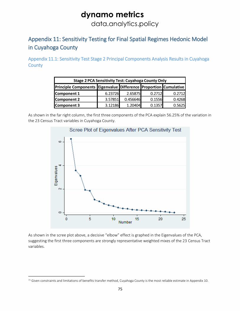
75
Appendix 11: Sensitivity Testing for Final Spatial Regimes Hedonic Model
in Cuyahoga County
Appendix 11.1: Sensitivity Test Stage 2 Principal Components Analysis Results in Cuyahoga County
As shown in the far right column, the first three components of the PCA explain 56.25% of the variation in
the 23 Census Tract variables in Cuyahoga County.
As shown in the scree plot above, a decisive “elbow” effect is graphed in the Eigenvalues of the PCA,
suggesting the first three components are strongly representative weighted mixes of the 23 Census Tract
variables.
71 Given constraints and limitations of benefits transfer method, Cuyahoga County is the most reliable estimate in Appendix 10.
Principle Components Eigenvalue Difference Proportion Cumulative
Component 1 6.23726 2.65875 0.2712 0.2712
Component 2 3.57851 0.456646 0.1556 0.4268
Component 3 3.12186 1.20404 0.1357 0.5625
Stage 2 PCA Sensitivity Test: Cuyahoga County Only
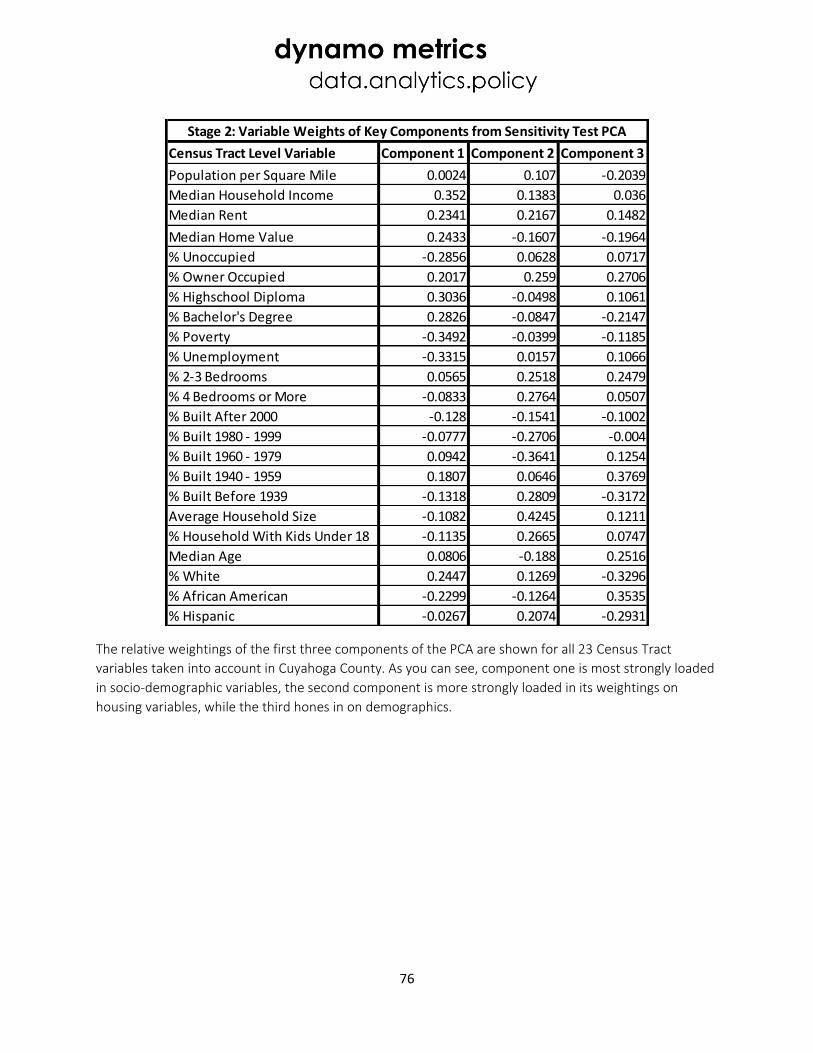
76
The relative weightings of the first three components of the PCA are shown for all 23 Census Tract
variables taken into account in Cuyahoga County. As you can see, component one is most strongly loaded
in socio-demographic variables, the second component is more strongly loaded in its weightings on
housing variables, while the third hones in on demographics.
Census Tract Level Variable Component 1 Component 2 Component 3
Population per Square Mile 0.0024 0.107 -0.2039
Median Household Income 0.352 0.1383 0.036
Median Rent 0.2341 0.2167 0.1482
Median Home Value 0.2433 -0.1607 -0.1964
% Unoccupied -0.2856 0.0628 0.0717
% Owner Occupied 0.2017 0.259 0.2706
% Highschool Diploma 0.3036 -0.0498 0.1061
% Bachelor's Degree 0.2826 -0.0847 -0.2147
% Poverty -0.3492 -0.0399 -0.1185
% Unemployment -0.3315 0.0157 0.1066
% 2-3 Bedrooms 0.0565 0.2518 0.2479
% 4 Bedrooms or More -0.0833 0.2764 0.0507
% Built After 2000 -0.128 -0.1541 -0.1002
% Built 1980 - 1999 -0.0777 -0.2706 -0.004
% Built 1960 - 1979 0.0942 -0.3641 0.1254
% Built 1940 - 1959 0.1807 0.0646 0.3769
% Built Before 1939 -0.1318 0.2809 -0.3172
Average Household Size -0.1082 0.4245 0.1211
% Household With Kids Under 18 -0.1135 0.2665 0.0747
Median Age 0.0806 -0.188 0.2516
% White 0.2447 0.1269 -0.3296
% African American -0.2299 -0.1264 0.3535
% Hispanic -0.0267 0.2074 -0.2931
Stage 2: Variable Weights of Key Components from Sensitivity Test PCA
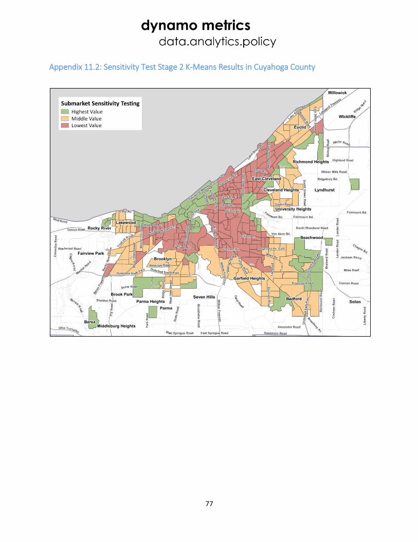
77
Appendix 11.2: Sensitivity Test Stage 2 K-Means Results in Cuyahoga County
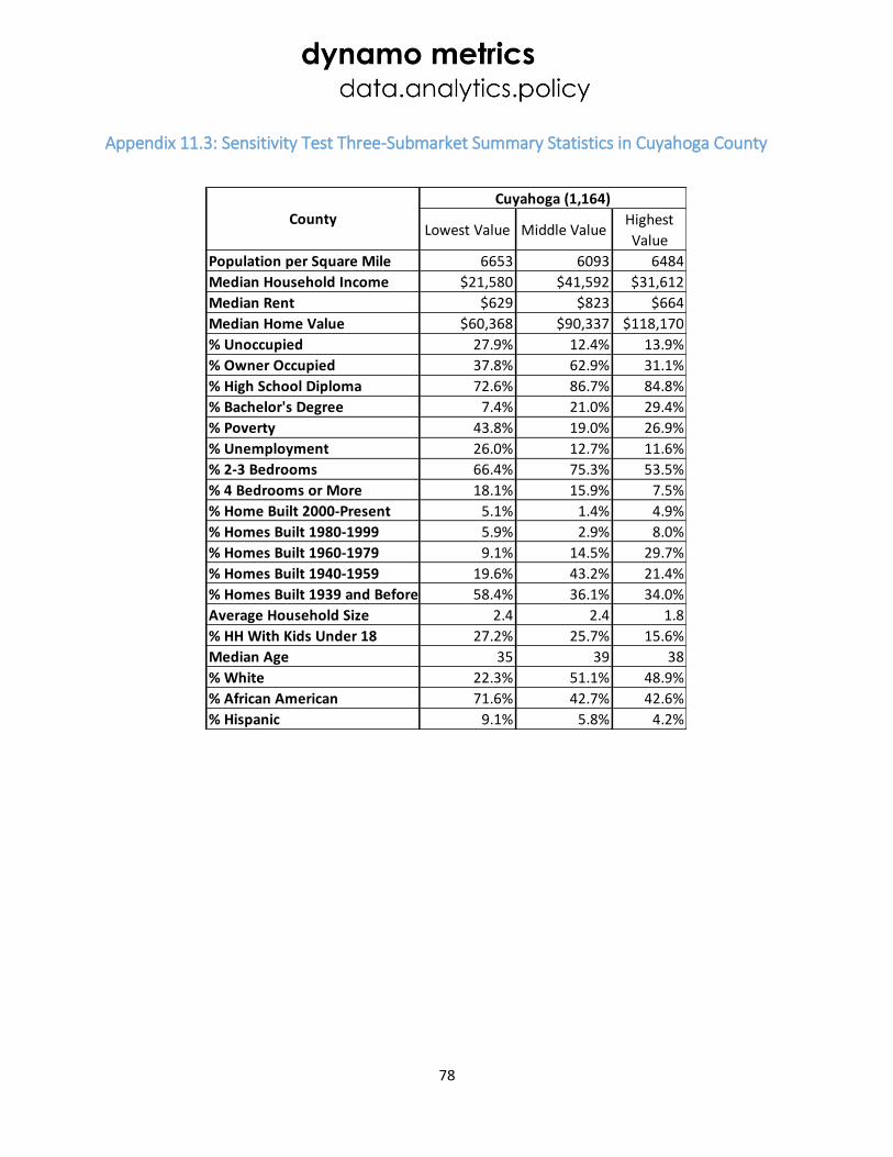
78
Appendix 11.3: Sensitivity Test Three-Submarket Summary Statistics in Cuyahoga County
Lowest Value Middle ValueHighest
Value
Population per Square Mile 6653 6093 6484
Median Household Income $21,580 $41,592 $31,612
Median Rent $629 $823 $664
Median Home Value $60,368 $90,337 $118,170
% Unoccupied 27.9% 12.4% 13.9%
% Owner Occupied 37.8% 62.9% 31.1%
% High School Diploma 72.6% 86.7% 84.8%
% Bachelor's Degree 7.4% 21.0% 29.4%
% Poverty 43.8% 19.0% 26.9%
% Unemployment 26.0% 12.7% 11.6%
% 2-3 Bedrooms 66.4% 75.3% 53.5%
% 4 Bedrooms or More 18.1% 15.9% 7.5%
% Home Built 2000-Present 5.1% 1.4% 4.9%
% Homes Built 1980-1999 5.9% 2.9% 8.0%
% Homes Built 1960-1979 9.1% 14.5% 29.7%
% Homes Built 1940-1959 19.6% 43.2% 21.4%
% Homes Built 1939 and Before 58.4% 36.1% 34.0%
Average Household Size 2.4 2.4 1.8
% HH With Kids Under 18 27.2% 25.7% 15.6%
Median Age 35 39 38
% White 22.3% 51.1% 48.9%
% African American 71.6% 42.7% 42.6%
% Hispanic 9.1% 5.8% 4.2%
County
Cuyahoga (1,164)
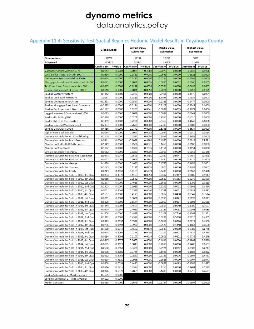
79
Appendix 11.4: Sensitivity Test Spatial Regimes Hedonic Model Results in Cuyahoga County
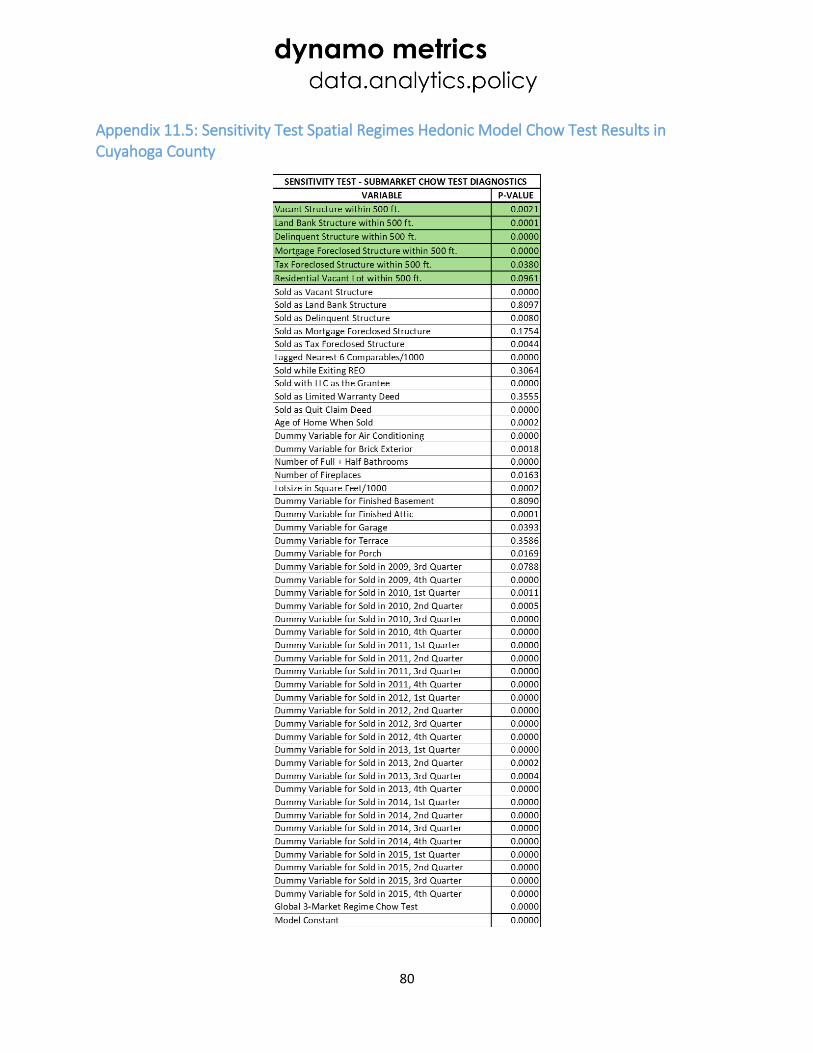
80
Appendix 11.5: Sensitivity Test Spatial Regimes Hedonic Model Chow Test Results in Cuyahoga County