Embed Size (px)
Citation preview
ESTIMATING DENSITY OF FLORIDA KEY DEER
A Thesis
by
CLAY WALTON ROBERTS
Submitted to the Office of Graduate Studies of Texas A&M University
in partial fulfillment of the requirements for the degree of
MASTER OF SCIENCE
May 2005
Major Subject: Wildlife and Fisheries Sciences
ESTIMATING DENSITY OF FLORIDA KEY DEER
A Thesis
by
CLAY WALTON ROBERTS
Submitted to Texas A&M University in partial fulfillment of the requirements
for the degree of
MASTER OF SCIENCE
Approved as to style and content by:
Ro(C
No(M
el R. Lopez hair of Committee)
va J. Silvy ember)
Steven G. Whisenant (Member)
Robert D. Brown (Head of Department)
May 2005
Major Subject: Wildlife and Fisheries Sciences
iii
ABSTRACT
Estimating Density of Florida Key Deer.
(May 2005)
Clay Walton Roberts, B.S., Texas A&M University
Chair of Advisory Committee: Dr. Roel Lopez
Florida Key deer (Odocoileus virginianus clavium) were listed as endangered by
the U.S. Fish and Wildlife Service (USFWS) in 1967. A variety of survey methods have
been used in estimating deer density and/or changes in population trends for this species
since 1968; however, a need to evaluate the precision of existing and alternative survey
methods (i.e., road counts, mark-recapture, infrared-triggered cameras [ITC]) was
desired by USFWS.
I evaluated density estimates from unbaited ITCs and road surveys. Road
surveys (n = 253) were conducted along a standardized 4-km route each week between
January 1999–December 2000 (total deer observed, n = 4,078). During this same period,
11 ITC stations (1 camera/42 ha) collected 5,511 deer exposures. Study results found a
difference (P < 0.001) between methods with road survey estimates lower (76 deer) than
ITC estimates (166 deer). Comparing the proportion of marked deer, I observed a higher
(P < 0.001) proportion from road surveys (0.266) than from ITC estimates (0.146).
Lower road survey estimates are attributed to (1) urban deer behavior resulting in a high
proportion of marked deer observations, and (2) inadequate sample area coverage. I
iv
suggest that ITC estimates are a reliab alternative to road surveys for
estimating Key deer densities on outer island
I also evaluated ds. Road survey
methods (n = 100) were conducted alo ized 31-km route where mark-
resight, strip-trans n June 2003–
May 2004. I found mark-resight estimates to be lower (
le and precise
s.
density estimates from 3 road survey metho
ng a standard
ect, and distance sampling data were collected betwee
x = 384, 95% CI = 346–421)
than strip-transect estimates ( x = 854, 95% CI = 806–902) and distance estimates ( x =
523, 95% CI = 488–557). I attribute low mark-resight estimates to urban deer behavior
resulting in a higher proportion of marked deer observations along roadways. High
strip-transect estimates also are attributed to urban deer behavior and a reduced effective
strip width due to dense vegetation. I propose that estimates using distance samplin
eliminate some of these
g
biases, and recommend their use in the future.
v
DEDICATION
I dedicate this to my Mom and Dad who taught me that the journey is more
important than the destination; and, to my Grandmother and Stepmother who always
have time to share a cup of coffee. Also, to my Brother who shares my passion for he
outdoors and history.
t

vi
ACK NTS
like to thank the members of my committee, Roel Lopez and Nova Silvy,
idance through my graduate school experience. The lessons I learned from
, many of which had nothing to do with scholastic improvement or Key deer
biology, w g
hard, having fun, and promoting positive ener
a
me kicking and screaming up to a higher stan
ecology and research.
Secondly, I would like to express my ppreciation to my fellow graduate students
in the Department of Wildlife and Fisheries Sciences (WFSC) at Texas A&M
University, colleagues at the National Key Deer Refuge, The Nature Conservancy,
Mosquito Control, and Mote Marine Institute, many of whom are friends, hunting
buddies, spear fishing buddies, rum drinking buddies, co-authors and co-conspirators; all
of whom made my experience at A&M and in the Keys unforgettable. Special thanks
have to be extended to the TAMU student interns, Americorps volunteers, and other
volunteers who assisted in the collection of field data.
Funding was provided by TAMU System, Rob and Bessie Welder Wildlife
Foundation, Florida Fish and Wildlife Conservation Commission, and USFWS (Special
Use Permit No. 97-14). Special thanks are extended to the staff of the National Key
Deer Refuge, Monroe County, Florida. Last, but certainly not least, thank you to the
ladies in the WFSC office that kept me in line all those years.
NOWLEDGME
I would
for their gu
them
ill not soon be forgotten. They understand the value and concepts of workin
gy with colleagues. Additionally, I would
lso like to thank Professors M. Peterson, S. Davis, and S. Whisenant who helped drag
dard of understanding of various aspects of
a

vii
TABLE OF CONTENTS
ii
I
2 .. 3
5
8
15 19
MA ING WHITE- 21
25 28 32 34
Page
ABSTRACT ...................................................................................................... i
DEDICATION .................................................................................................. v
ACKNOWLEDGMENTS................................................................................. vi
TABLE OF CONTENTS .................................................................................. vii
LIST OF FIGURES........................................................................................... ix
LIST OF TABLES ............................................................................................ xii
CHAPTER
INTRODUCTION .............................................................................. 1
Objectives ............................................................................... Study Area ............................................................................
II COMPARISON OF CAMERA AND ROAD SURVEY ESTIMATES FOR WHITE-TAILED DEER............................................................
Synopsis .................................................................................. 5 Introduction............................................................................. 6 Methods .................................................................................. Results..................................................................................... 13 Discussion............................................................................... Management Implications.......................................................
III COMPARISON OF 3 METHODS IN ESTI TTAILED DEER DENSITY ................................................................
Synopsis .................................................................................. 21 Introduction............................................................................. 22 Methods .................................................................................. Results..................................................................................... Discussion............................................................................... Management Implications.......................................................

viii
C Page HAPTER
ESTIMATING KEY DEER DENSITY ............................................. 35
Historical Surveys .................................................................. 35
IV SUMMARY AND SURVEY RECOMMENDATIONS FOR
Survey Recommendations ...................................................... 39
LITERATURE CITED...................................................................................... 54
APPENDIX A ................................................................................................... 63
VITA.................................................................................................................. 69
ix
LIST OF FIGURES
FIGUR Page
1 nge he endangered Florida Key deer, Monroe County,
2
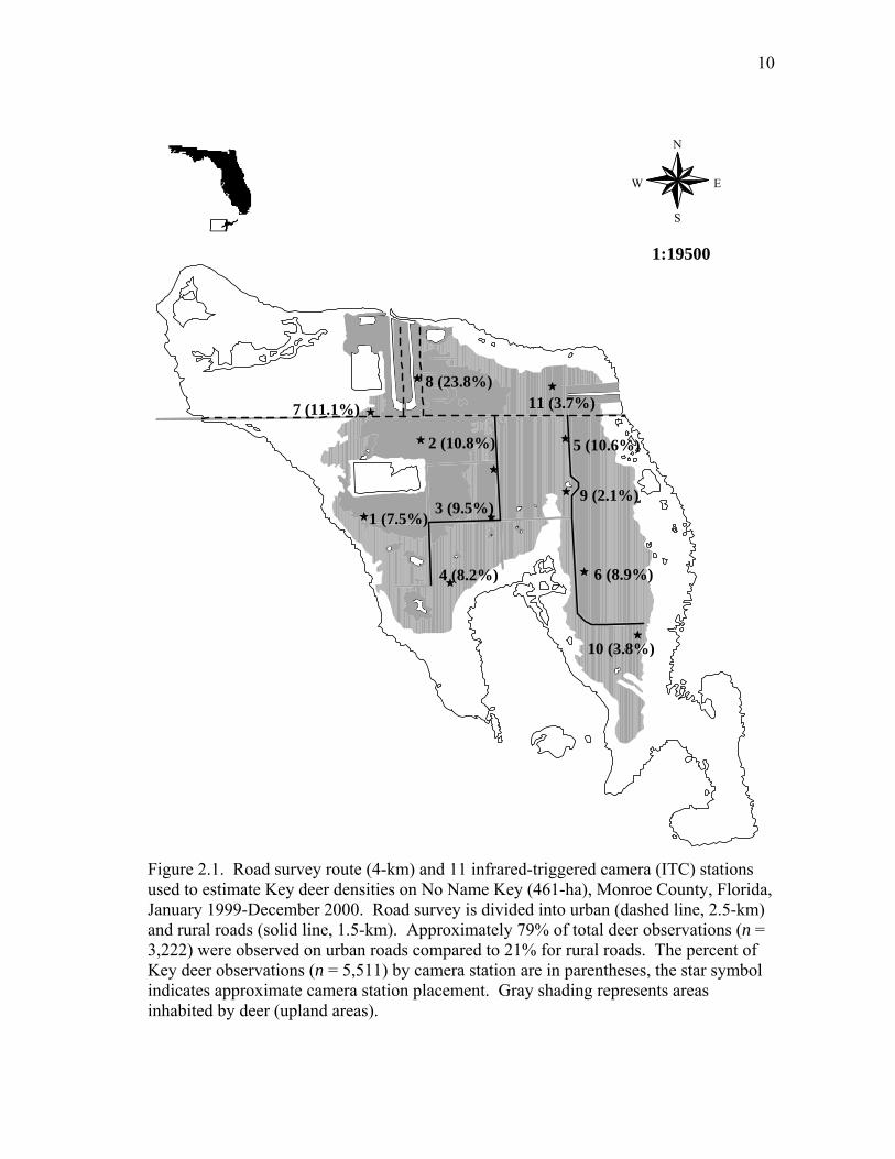
rvey route (4-km) and 11 infrared-triggered camera (ITC)
(461-ha), Monroe County, Florida, January 1999-December
and rural roads (solid line, 1.5-km). Approximately 79% of total
compared to 21% for rural roads. The percent of Key deer observations (n = 5,511) by camera station are in parentheses, the star symbol indicates approximate camera station placement. Gray shading represents areas i habited by deer (upland areas)….
10
2.2 Florida Key deer density estim ean, SE) by season, time of day (sunrise=SR, sunset=SS, nighttime=NT), and method (road survey, infrared-triggered camera estimates [ITC]) for No Name Key (461-ha), Monroe County, Florida, January 1999-December 2000.………………………………………………………………
16
2.3 Simpson’s index of evenness fo individually marked Florida Key deer (n = 19, n = 12 females, n = 7 males) by method for No Name Key, Monroe County, Florida, January 1999-December 2000.…………………………………………......
17
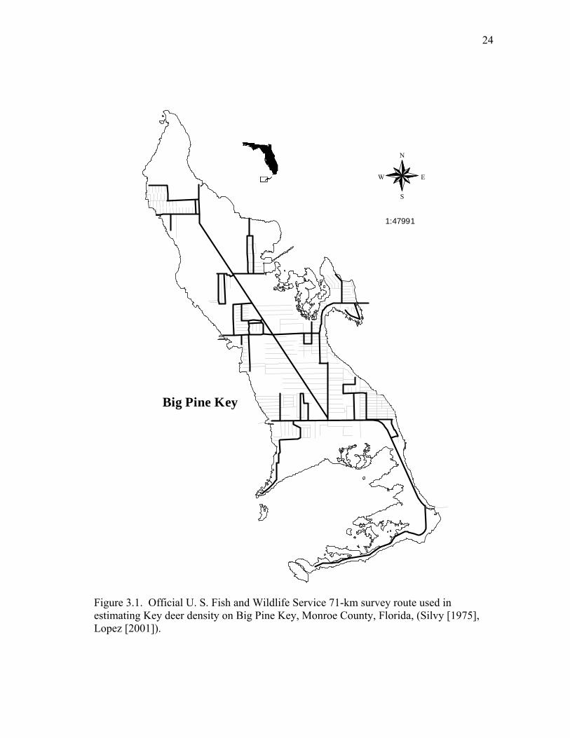
3.1 Official U. S. Fish and Wildlife Service 71-km survey route used in estimating Key deer density n Big Pine Key, Monroe County, Florida, (Silvy [1975], Lopez [2001])…………………………….
24
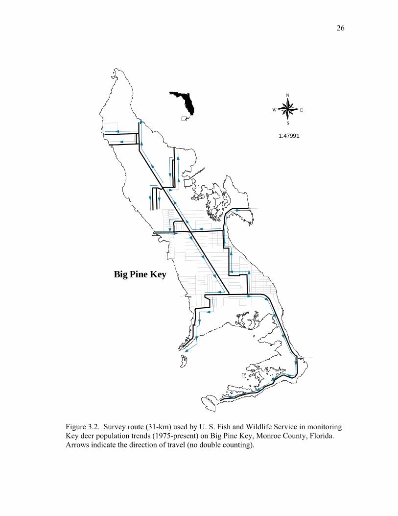
3.2
Survey route (31-km) used by U. S. Fish and Wildlife Service in monitoring Key deer population trends (1975-present) on Big Pine Key, Monroe County, Florida. Arrows indicate the direction of travel (no double counting)…...………………………………..
26
E
.1 Ra of tFlorida....…..................................................................................... 4
.1 Road su
stations used to estimate Key deer densities on No Name Key
2000. Road survey is divided into urban (dashed line, 2.5-km)
deer observations (n = 3,222) were observed on urban roads
n
ates (m
r observations from
o

x
FIGURE Page
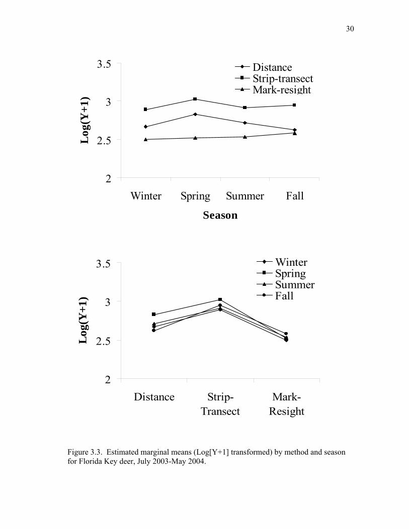
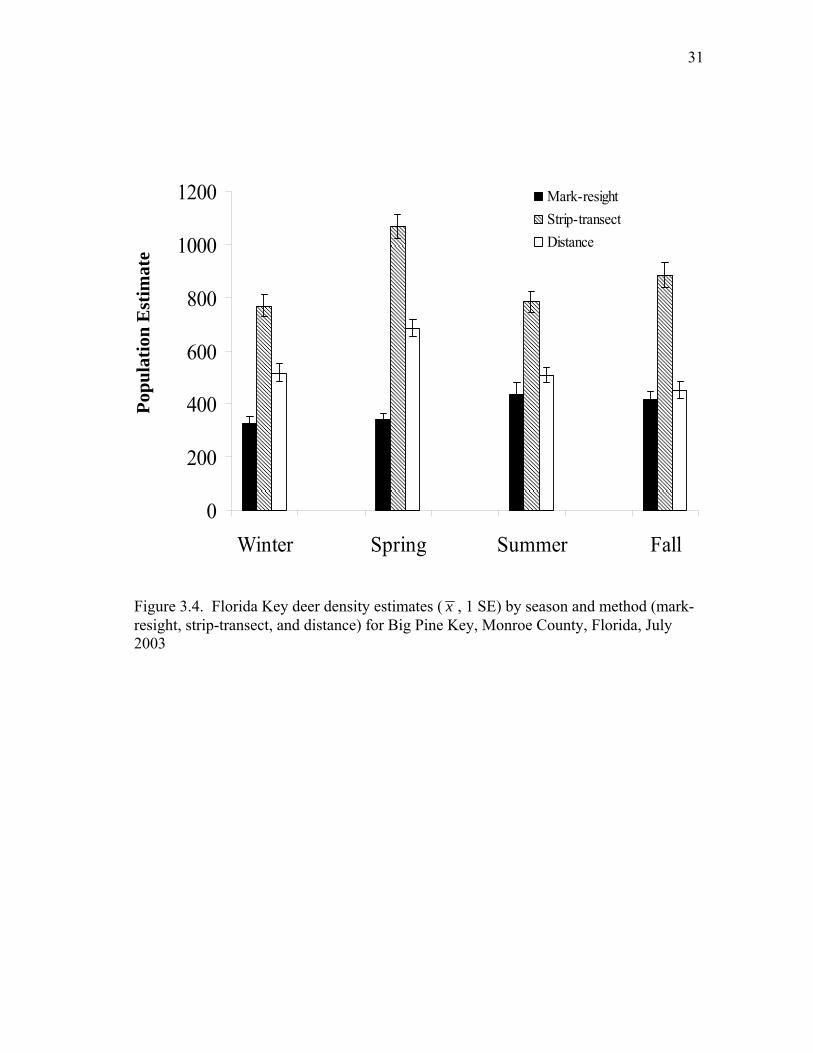
and season for Florida Key deer, July 2003-May 2004…………... 30
3.4
3.3 Estimated marginal means (Log[Y+1] transformed) by method
Florida Key deer density estimates (
x , 1 SE) by season and method (mark-resight, strip-transect, and distance) for Big Pine
31
.1 BPK
….
37
.2
44
4.4
46
4.5
48
4.6
49
Key, Monroe County, Florida, July 2003…………………………
Original survey routes (BPK 44-mile, solid and dotted lines; 10-mile, dotted line only; NNK [1998-2001]) used in estimatingKey deer density on Big Pine (BPK) and No Name (NNK) keys, 1968-1972 (Silvy 1975), 1998-2001 (Lopez 2001)……………
Official U. S. Fish and Wildlife Service (USFWS) survey route used in monitoring Key deer population trends on Big Pine BPK) and No Name (NNK) keys, 1975-present…………………
4
4
( The TAMU/FWS 19-mile route used in estimating Key deer density on Big Pine (BPK), 2003-2004…………………………... Proposed survey route for future Key deer monitoring by the U.S.
ish and Wildlife Service (USFWS). Survey route is slightly
38
4.3
Fmodified from the official USFWS route (Figure 2), accounting for recent road closures and high density developments. Arrows indicate the direction of travel (no double counting)……………...
elative size comparison of Florida Key deer by sex and age.
RHead shapes vary between adults (size of egg plant), yearlings (size of papaya), and fawns (size of mango)……………………...
ody comparison of adult female (top) and male (bottom) Florida
BKey deer. Note elongated head, rectangular bodies, and, in the case of the males, hardened antlers and swollen neck…………….

xi
FIGURE Page
Key deer. Note male head shape after dropping antlers…………. 50
4.8 male Key deer…………………………………………………
51
4.7 Head comparison of adult female (left) and male (right) Florida
Comparison of body size and head shape for 3 age-classes of fe

xii
LIST OF TABLES
TABLE Page
4.1 verage Key deer observed by survey route and year, Big Pine ….
40
Aand No Name keys, 1969-2001..………………………………
1
CHAPTER I
INTRODUCTION
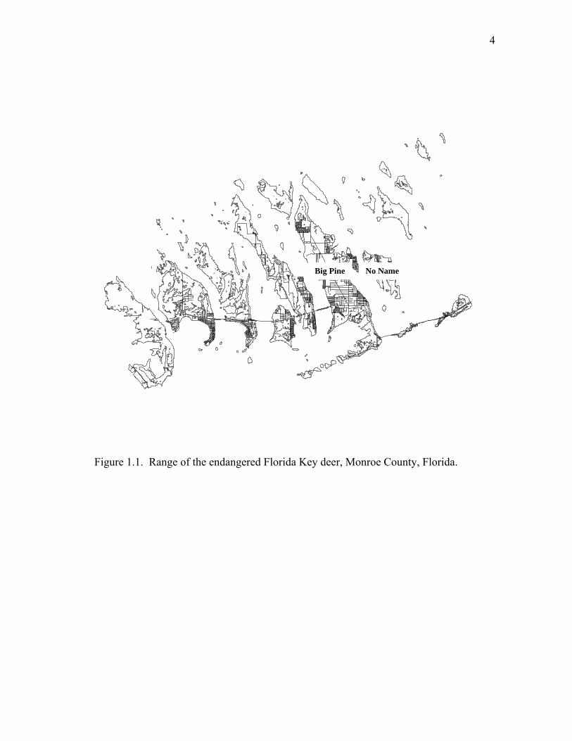
Th e led er i
the United States, are endemic to the Lower Florida Keys (Hardin et al. 1984). Key deer
occupy 20-25 islands within the boundaries of the National Key Deer Refuge (NKDR)
with the majority of the population (≈75%) found on Big Pine (BPK) and No Name
(NNK; Fig. 1.1; Lopez 2001) keys. The most recent population estimate indicates
approximately 500 Key deer on BPK and NNK (Lopez 2001), an increase from the
estimated 30–50 deer in the late 1940s.
The need for wildlife managers to obtain reliable population estimates is
paramount in the field of wildlife ecology. Managers need practical, field-tested
techniques that are repeatable and can be used by a variety of field personnel (Koenen et
al. 2002). Estimating abundance or density of an animal population is important for
developing proper conservation policy and management protocols (Gelatt and Siniff
1999, Swann et al. 2002), particularly with threatened or endangered species like the
Florida Key deer. Annual population monitoring is mandated in the current Key Deer
Recovery Plan (U. S. Fish and Wildlife Service [USFWS] 1999).
Traditional methodologies such as drive, strip, aerial, thermal/infrared counts,
and mark-capture techniques can be expensive, labor intensive, or limited to habitats
with high visibility and lack of dense cover (Lancia et al. 1994, Jacobson et al. 1997,
Jachmann 2002). Since 1968, spotlight counts have been conducted on the Florida Key
e ndangered Florida Key deer, the smallest subspecies of white-tai de n
The format and style of this thesis follows Journal of Wildlife Management.
2
deer (Silvy 1975, Lopez 2001) to mo trends (index). Efforts to estimate
population density (deer/unit area) limited to mark-resight efforts
m
OBJEC
te
I compared distance
samplin
future monitoring efforts with Key deer. My thesis is divided into 3 chapters:
nitor population
, however, have been
conducted in 1968-1972 and 1998-2001 (Silvy 1975, Lopez 2004). Use of mark-resight
methodologies are labor intensive and expensive, and may be impractical in the annual
monitoring of Key deer by USFWS biologists. A need to evaluate alternative methods
of estimating Key deer density is necessary, particularly methods that are easy to
implement, precise, and economical. Furthermore, methods that provide USFWS
biologists with annual density estimates rather than population trends (e.g., index fro
spotlight counts) would be preferred.
TIVES
The objective of my thesis was to evaluate 2 alternative methods to estima
population density for the endangered Florida Key deer. First, I evaluated the use of
infrared-triggered cameras (ITC) in estimating deer numbers (Kucera et al. 1995,
Jacobson et al. 1997, Koerth and Kroll 2000) compared to traditional mark-resight
methods to assess the applicability of ITCs in estimating Key deer densities on outer
islands. Alternative methods of estimating Key deer densities on outer keys where the
lack of roads precludes traditional road counts are needed. Second,
g (Buckland et al. 1993, Corn and Conroy 1998, Tomas et al. 2001, Forcardi et
al. 2002a, Koenen et al. 2002, Swann et al. 2002, Ransom and Pinchak 2003), strip-
transect (Burnham and Anderson 1984, Johnson and Rutledge 1985, Hiby and Krishna
2001), and mark-resight methodologies to evaluate the usefulness of these methods in

3
1. Use of infrared-triggered cameras in estimating Key deer (Chapter II).
2. Comparison of distance sampling, strip-transects, and mark-resight methods in
estimating Key deer (Chapter III).
3. Final recommendations for estimating Key deer (Chapter IV).
STUDY AREA
The Florida Keys extend 200 km from the southern tip of peninsular Florid
1.1). Soils vary from marl deposits to bare rock of the oolitic limestone formation
(Dickson 1955). Typically, island areas near sea level (maritime zones) are comprised
of red mangrove (Rhizophora mangle),
a (Fig.
black mangrove (Avicennia germinans), white
cularia racemosa), and buttonwood (Conocarpus erecta) forests. With
n
d
mangrove (Lagun
increasing elevation, maritime zones transition into hardwood (e.g., gumbo limbo
[Bursera simaruba], Jamaican dogwood [Piscidia piscipula]) and pineland (e.g., slash
pine [Pinus elliottii], saw palmetto [Serenoa repens]) upland forests with vegetatio
intolerant of salt water (Dickson 1955, Folk 1991). Two islands, BPK (2,548 ha) an
NNK (461 ha), were selected in my study because (1) the majority of the Key deer
population (≈ 75%, Lopez 2001, Lopez 2004) reside on these 2 islands, and (2) long-
term population survey data have been collected on these 2 islands (Silvy 1975, Lopez
2004).
4
Figure 1.1. Range of the endangered Florida Key deer, Monroe County, Florida.
Big Pine No Name
5
CHAPTER II
COMPARISON OF CAMERA AND ROAD SURVEY ESTIMATES FOR
WHITE-TAILED DEER
SYNOPSIS
Wildlife managers require reliable, cost effective, and accurate methods for
conducting population surveys in making wildlife management decisions. Traditional
methods such as spotlight counts, drive counts, strip counts (aerial, thermal, infrared)
and mark-recapture techniques can be expensive, labor inten imited to habitats
with high visibility. Convenience sampling designs are often used to circumvent these
problems, creating the potential for unknown bias in survey results. Infrared-triggered
cameras (ITCs) are a rapidly developing technology that may provide a viable
alternative to wildlife managers, as they can be economically used within a random
sampling design. I evaluated population density estimates from unbaited ITCs and road
surveys for the endangered Florida Key deer on No Name Key, Florida (461-ha island).
Road surveys (n = 253) were conducted along a standardized 4-km route each week at
sunrise (n = 90), sunset (n = 93), and nighttime (n = 70) between January 1999–
ecember 2000 (total deer observed, n = 4,078). During this same period, 11 ITC
tations (1 camera/42 ha) collected 8,625 exposures, of which 5,511 registered deer
4% of photographs). Study results found a difference (P < 0.001) between methods
ith road survey population estimates lower (76 deer) than from ITC estimates (166
eer). In comparing the proportion of marked deer between the 2 methods, I observed a
igher (P < 0.001) proportion from road surveys (0.266) than from ITC estimates
sive, or l
D
s
(6
w
d
h
6
(0.146). Spatial analysis of deer obs ealed the sample area coverage to
be in ere
on urban roads which comprised 63% of the survey route. Lower road survey estimates
to (1) urban deer behavior resulting in a high proportion of marked deer
are
rly
ogy
ost
aefer
s
ervations also rev
congruent between the 2 methods; approximately 79% of all deer observations w
are attributed
observations, and (2) inadequate sample area coverage. I suggest that ITC estimates
a reliable and precise alternative to road surveys for estimating white-tailed deer
densities, and may alleviate sample bias generated by convenience sampling, particula
on small, outer islands where habitat and/or lack of infrastructure (i.e., roads) precludes
the use of other methods.
INTRODUCTION
Reliable population estimates are paramount in the field of wildlife ecol
(Jenkins and Marchinton 1969) because assessment of “the stock on hand” is a
prerequisite for many wildlife management endeavors (Leopold 1933). Population
density estimates are important for implementing harvest strategies or in developing
proper conservation policy and management protocols (Gelatt and Siniff 1999, Koenen
et al. 2002, Swann et al. 2002). Since white-tailed deer (O. virginianus) are the m
economically important big game mammal in North America (Beechinor 1986, Sch
and Main 2001), obtaining reliable population estimates is both a necessary and
worthwhile component of white-tailed deer management. Reliable population estimate
are even more important with threatened or endangered species, like the Florida Key
deer whose recovery efforts require annual population monitoring (U. S. Fish and
Wildlife Service [USFWS] 1999).

7
Traditional methodologies such as drive counts, strip counts (aerial, thermal,
infrared), and mark-recapture techniques can be expensive, labor intensive, or limited to
habitats with high visibility (Lancia et al. 1994, Jacobson et al. 1997). As a result,
sampling designs often are altered to obtain estimates in a non-random fashion, which
lowers the cost and/or effort required to obtain the estimate. Convenience sampling of
this sort has been criticized widely within the literature due to the probability of b
is inherent to this type of sample design (Anderson 2001, Mackenzie and Kendall 2002,
Thompson 2002, Anderson 2003, Ellingson and Lukacs 2003). Of greater concern is the
lack of evidence to either
ias that
validate the assumption that the sample is not biased by
g or to determine the amount and/or direction of bias resulting from
at may
ior
evious
ark-resight methods is that all animals have “equal
convenience samplin
the non-random sampling design.
Infrared-triggered cameras (ITCs) are a rapidly developing technology th
provide a viable alternative to wildlife managers as they can be economically used
within a random or systematic sampling design. Due to their relatively small size,
automated function, and robust sampling duration, ITCs can be used to conduct
population surveys (Mace et al. 1994, Jacobson et al. 1997) and to study animal behav
and movements (Savidge and Seibert 1988, Carthew and Slater 1991, Mason et al. 1993,
Foster and Humphrey 1995, Karanth 1995, Karanth and Nichols 1998). While pr
research (Kucera et al. 1995, Jacobson et al. 1997, Koerth and Kroll 2000) suggests that
ITCs are a useful means for estimating population densities, these studies were
conducted using baited camera sites which may introduce unwanted bias in the
estimates. A basic assumption of m

8
catchability” (Krebs 1999), which may not be the case when using bait to draw animals
into the sample area. Information on the utility of estimating white-tailed deer numbers
with randomly placed, unbaited, ITCs is needed. Furthermore, mark-resight estima
from traditional road surveys and ITCs should be evaluated, including similarities in
animal sightability between methods (i.e., “equal catchability”).
I compared estimates from traditional road surveys and ITCs for a marked island
population of white-tailed deer. Florida Key deer are an endangered subspecies of
white-tailed deer endemic to the Lower Florida Keys (Hardin et al. 1984). The Key deer
population on No Name Key (461 ha) provided me with a unique opportunity to (1
compare estimates from unbaited ITCs to road surveys and (2) to evaluate the proportion
of marked deer between the 2 meth
tes
)
ods. Comparable results would provide a precedent
for usin
dition
were
g ITCs to estimate deer densities on the outer islands where a lack of roads
precludes the use of traditional road surveys.
METHODS
Trapping and Marking
Deer were captured and marked on No Name Key between January 1999–
December 2000 using portable drive nets (Silvy et al. 1975), drop nets (Lopez et al.
1998), and hand capture (Silvy 1975, Lopez 2001). Deer were physically restrained
after capture with an average holding time of 10–15 minutes (no drugs were used). Sex,
age, capture location, body weight, radio frequency (if applicable), and body con
were recorded for each deer prior to release (Lopez et al. 2003b). Captured deer
marked with plastic neck collars (8-cm wide) for adult and yearling females, leather
9
antler collars (0.25-cm wide) for yearling and adult males and elastic expandable neck
collars for (3-cm wide) for fawns (Lopez et al. 2004a). Neck collars were equipped with
plastic ear tags for easy identification at a distance; 67–75% of the marked deer were
equipped with radio transmitters (Lopez et al. 2004a). Captured deer also were given
ear tattoo that served as a permanent marker (Silvy 1975).
an
arked), location, sex, and age
g, adult) on a map of the survey route (Lopez et al. 2004a). Deer were not
ortions of the road to alleviate the problem of double
g
Road Surveys
Weekly road counts were conducted along a standardized 4-km route on No
Name Key at sunrise, sunset, and nighttime from January 1999–December 2000 (Fig.
2.1, Lopez et al. 2004a). Start and finish points were the same for each survey route.
Sunrise surveys started 30 minutes before sunrise. Sunset surveys started 1.5 hours
before sunset, and night surveys were conducted about 1 hour after sunset. Two
observers in a vehicle traveled along the survey route (average travel speed 16–24
km/hr) and recorded the observed number (marked/unm
(fawn, yearlin
counted on the backtrack p
counting. Survey data were entered into an Access database and Arcview GIS for
further analysis (Lopez 2001).
Camera Surveys
Eleven TrailMaster 1500 Active Infrared Trail Monitors (TrailMaster,
Goodson and Associates, Inc., Lenexa, KS, USA) consisting of a transmitter, receiver,
and a 35-mm camera were placed following a systematic design (Fig. 2.1). First, I
restricted camera placement to upland Key deer habitats (Lopez et al. 2004b), avoidin
10
1:19500
tions
used to estimate Key deer densities on No Name Key (461-ha), Monroe County, Florida,
and rural roads (solid line, 1.5-km). Approximately 79% of total deer observations (n = of
Key deer observations (n = 5,511) by camera station are in parentheses, the star symbol
inhabited by deer (upland areas).
Figure 2.1. Road survey route (4-km) and 11 infrared-triggered camera (ITC) sta
January 1999-December 2000. Road survey is divided into urban (dashed line, 2.5-km)
3,222) were observed on urban roads compared to 21% for rural roads. The percent
indicates approximate camera station placement. Gray shading represents areas
ÊÚ
ÊÚÊÚ
ÊÚ
ÊÚ
ÊÚÊÚ
ÊÚ
ÊÚ
ÊÚ
ÊÚ
ÊÚ
7 (11.1%) 11 (3.7%)
2 (10.8%) 5 (10.6%)
10 (3.8%)
8 (23.8%)
9 (2.1%)
6 (8.9%)
3 (9.5%)
4 (8.2%)
1 (7.5%)
N
EW
S
11
mangrove and buttonwood areas that are influenced by tides and not used by deer. I then
divided inhabited areas into approximately 42-ha blocks (slightly higher camera density
uggested by Jacobson et al. 1997); each block was then searched until a suitable (e.g.,
ell used deer trail, waterhole) camera location was found. Camera stations collected
ata from January 1999–December 2000. Cameras were set to take pictures throughout
e day (0001–2400 hours) with a delay inutes. The number of
arked and unmarked animals including the animal’s ear tag number, sex, age, and
cation were recorded and entered into an Access database.
ata Analysis
I determined weekly population estimates using a using Lincoln-Petersen
eber’s modification) estimator for road surveys (White et al. 1982, Krebs 1999, Lopez
t al. 2004a) and ITC data (Lincoln-Petersen, Seber’s modification estimator, Krebs
999). Population data (road surveys and photographs) met the requirements for this
stimate because (1) the population was closed (i.e., study area is an island, with limited
ispersal between islands and small population growth, Lopez et al. 2004a), and (2) a
egment of the population was marked for individual identification during the study.
he marked population (approximately 67–75% of marked population included radio
s
w
d
th between pictures of 30 m
m
lo
D
(S
e
1
e
d
s
T
transmitter) allowed us to readjust the number of available marked deer each week from
telemetry data or survey data observations. Deer observations from ITC stations were
pooled to determine a weekly population estimate.
12
Weekly estimates were randomly selected from both methods to generate a
.
n methods (road, ITC),
summer, fall, winter), and years (1999, 2000) using a 1 within-subjects
001).
s
f
parately for each year using the
estimated marginal means for all 4 seasonal categories (SPSS 2001). For each weekly
balanced design which maximized the number of surveys within each season x method x
year treatment combination. I applied the Lilliefors significance modification to the
Kolmogorov-Smirnov test to determine if the data were normally distributed. Levene’s
test for equal variance among treatment groups, followed by a spread versus level
diagnostic regression (modified Box-Cox algorithm; SPSS 2001), was used to determine
if a variance stabilizing transformation would be needed. Results indicated that a
log(Y+1) transformation was required to meet assumptions of a parametric ANOVA
I tested for differences in population estimates betwee
seasons (spring,
factor, 2 between-subjects factor, split-plot (repeated measures) ANOVA (SPSS 2
Seasons were defined as winter (January–March [pre-fawning season]), spring (April–
June [fawning season]), summer (July–September [pre-breeding season]), and fall
(October–December [breeding season], Lopez et al. 2004a). Repeated-measures
ANOVA designs account for lack of independence when repeated observations are
obtained from the same experimental units (Tzilkowski and Storm 1993, Zar 1996,
Lomax 2001, von Ende 2001). Because there were only 2 levels for the within-subject
factor (year), compound symmetry was assured (i.e., only 1 covariance). As such,
adjusted F-test (Geisser and Greenhouse 1958, Huynh and Feldt 1976) and MANOVA
techniques (no compound symmetry assumption) were not required for the evaluation o
these data. Results for each method were plotted se
13
estimat
neck co
0
e, I compared the proportion of marked deer (number marked/total deer
observed) between methods using an independent Student’s t-test (SPSS 2001). All
statistical comparisons were conducted at α = 0.05.
I compared the “sightability” of individually marked Florida Key deer between
road and camera surveys using Simpson’s index of evenness (Krebs 1999). The
Simpson’s index of evenness (ED) describes the evenness of observations for an
individual among all observations (ED assumes a value between 0–1, with 1 being
completely even). I restricted my analysis to animals marked with neck collars (only
llars could be used to identify individual deer) and animals monitored for 12
months. I standardized the sampling period to avoid biases in the calculation of the
index due to differences in sampling effort.
RESULTS
Density Estimates
Road and ITC surveys were conducted from January 1999–December 200
except September 1999 due to the landing of Hurricane Irene (Lopez et al. 2003a). A
weekly average of 22 deer (with a range between 18 and 35) were maintained in my
marked herd. A total of 253 road surveys were conducted (sunrise n = 90, sunset n = 93,
nighttime n = 70) with 4,078 deer observations (male n = 1,411, female n = 2,246,
unknown n = 421). Eleven camera stations collected 8,625 exposures during the same
time period, with 5,511 of those photographs registering deer (64% of the total
photographs). Other camera exposures included mammalian (n = 172, 2%), deer
unknown (n = 670, 8%), misfires (n = 1,969, 23%), and other (n = 303, 4%).
14
After transformation, I obtained a non-significant result (P = 0.125) for L
Test of equal variance among treatment groups. The Kolmogorov-Smirnov test with
Lilliefors significance modification, revealed 2 of 16
evene’s
treatment combinations to be non-
normal (camera × winter × 1999 [P = 0.23], road × fall × 1999 [P = 0.040]). As
ANOVA is deemed robust to minor departures from normality, these treatments w
included in the analysis.
I found road survey estimates to be lower (
ere
x = 76, SE = 6.45) compared to
estimates (
ITC
x = 166, SE = 14.92). The repeated-measures ANOVA results for between
subject effects (i.e., method) revealed a significant difference between the 2 methods
< 0.001) but not between seasons (P = 0.439), and there were no method x season
interactions (P = 0.963) (Fig. 2.2). The within-sub
-
(P
ject effects results indicated there
ces (P = 0.046) in density estimates between years and no year x method
9); however, I found a significant (P = 0.004) interaction between
year x e
d a
were differen
interaction (P = 0.91
season. As a result, the estimates between seasons depend upon the year of th
survey. Finally, there was no year x method x season interaction (P = 0.159).
In comparing the proportion of marked deer between the 2 methods, I observe
higher (P < 0.001) proportion from road surveys ( x = 0.266, SE = 0.010) than from ITC
estimates ( x = 0.146, SE = 0.009). Unlike the ITC estimates which offered a more
uniform sample of the island (Fig. 2.1), deer observations collected on the road survey
also were biased towards urban roads. Approximately 79% of all deer observati
observed on urban roads which comprised 63% of the survey route (Fig. 2.1).
ons were
15
A total of 19 individually marked Key deer (n = 12 females, n = 7 males) met my
criteria (total camera observations = 377, total road survey observations = 389). I fou
the E
nd
9,
l.
n (1) the
effectiv
more
uniform s for the ITC surveys captured a larger
D estimates from camera surveys (male ED = 0.566, female ED = 0.677, total ED =
0.615, Fig. 2.3) were higher than road surveys (male ED = 0.333, female ED = 0.59
total ED = 0.509, Fig. 2.3) from individually marked Florida Key deer.
DISCUSSION
Road surveys have been the preferred method to estimate Key deer densities
and/or monitor population trends by NKDR biologists for the last 30 years. All previous
population data have been collected using road surveys due to their ease of application
and the limited time and man-power available to conduct these surveys (Lopez et a
2004a). In comparing road survey estimates to ITC estimates, however, my study
revealed a significant difference between the 2 methods for all seasons and years. ITC
estimates were nearly 2 times those of road survey estimates (Fig. 2.2). While my study
did reveal the anticipated results, it does demonstrate that convenience sampling can
easily bias survey results. I attribute differences in density estimates to biases i
e area sampled between methods, and (2) the proportion of marked animals
observed between methods.
Sampling Area
Spatial analysis of survey results found 79% of road survey observations
occurred on urban roads (63% of the survey route); whereas ITC estimates were more
uniformly distributed (Fig. 2.1). I propose the systematic sampling design (i.e.,
coverage) and use of non-baited site

16
Figure 2.2. Florida Key deer density estimates (mean, SE) by season, time of day
camera estimates [ITC]) for No Name Key (461-ha), Monroe County, Florida, Janua
(sunrise=SR, sunset=SS, nighttime=NT), and method (road survey, infrared-triggered ry
1999-December 2000.
0
50
0
Winter Spring Summer Fall
Season
Popu
l
100
15
250
atio
n D
it
200
300y
ens
Road SRRoad SSRoad NTITC

17
0
0.25
0.5
0.75
1
Male Female Total
Sim
pson
's Ev
enne
ss In
dex
CameraRoad
Figure 2.3. Simpson’s index of evenness for observations from individually marked
lorida Key deer (n = 19, n = 12 females, n = 7 males) by method for No Name Key,
FMonroe County, Florida, January 1999-December 2000.
18
nother difference observed in my study was the proportion of marked animals
observed between the 2 sampling methods. I found the proportion of marked animals
observed on road surveys was nearly double those obtained from ITC data. As a result,
density estimates from road survey data were biased low (Krebs 1999). I attribute this
difference to trapping methods used and deer behavior. First, many animals were
trapped and collared in areas that were large enough for trapping procedures to take
place (i.e., use of drop nets, Lopez et al. 1998), and as a result were often located in
portion of the spatial variability and was not biased by the road network, which is highly
correlated with urban development. Furthermore, urban roads in the northern area of
island (Fig. 2.1) were improved, 2-lane, paved roads frequently driven by tourists and
residents. Human-deer interactions were greatest along these roadways (e.g., urban deer
feed by tourists by roadways). Conversely, the rural roads in the southern area of island
(Fig. 2.1) were unimproved, single-lane, roads on bare limestone cap rock. Key deer
were rarely observed along these roadways because animals were less domesticated (i.e.,
“wild” deer) and typically fled into the brush when a vehicle approached. Access into
these areas is limited (rural roads provide access to NKDR lands). Use of road surveys
would require that deer observations be obtained over a wider percentage of the island.
The road survey sampling design used in my study, however, was dictated by roadway
infrastructure that was biased towards urban areas. The difference in the “effective”
sampling area is a classic example of bias which often results from convenience
sampling.
Proportion Marked
A
19
close proximity to the survey route. Likewise, in recent years Key deer have become
urbanized in response to the abundance of food and fresh water in and around housing
areas (Lopez et al. 2004b). In particular, Key deer have been observed to remain near
roads due to the propensity of visiting tourists that feed deer from their vehicles (R.
Lopez, Texas A&M University, personal observation). I propose that both of these
variables have resulted in a biased road survey sample due to an unequal distribution o
marked deer. The bias in sightability of individual marked deer (camera surveys, E
f
e
y
emain a viable method to estimate population numbers; however, biologists
tential biases. The use of ITC in estimating population numbers
mera
st-
D =
0.615; road surveys, ED = 0.509, Fig. 2.3) supports this idea. Collectively, I propose th
bias in sampling area and differences in sightability of marked deer between both
methods accounts for population estimate differences observed in my study.
MANAGEMENT IMPLICATIONS
My study demonstrates that ITC surveys can be used to carry out precise
population estimates without the limitations inherent to road surveys. Road surve
estimates r
should be aware of po
also should be applied with caution. Previous research with ITCs (Kucera et al. 1995,
Jacobson et al. 1997, Koerth and Kroll 2000) were conducted using baited camera sites
which also may introduce unwanted bias in the estimates similar to my road surveys
(i.e., “trap-happy” deer). In comparing ED values between methods, though road
observations were higher (road surveys, ED = 0.509, Fig. 3), an ED value < 1 for ca
observations of marked deer also suggests that ITC estimates were influenced by
roadway biases. Furthermore, the use of ITCs to monitor large areas may become co
20
prohibitive or logistically impractical. For example, the costs in collecting road survey
data was approximately $50/week (2 people, does not include vehicle, fuel, spotlights)
compared to $85/week for ITC surveys (1 person, 11 cameras; does not include vehicle
fuel, and ITC equipment, latter is a significant cost). Though the ITC surveys are mo
expensive, I suggest that ITC surveys can be cost-effective in the monitoring of the
endangered Key deer on small, outer islands and in other areas where habitat and/or lack
of infrastructure precludes the use of other methods. In addition, ITC surveys reduce
potential biases associated with convenience sampling, and can be used in areas where
road infrastructure does not exist. I also recommend that natural markers (i.e., antl
patterns, physical deformities/injuries) can be used in place of maintaining a m
,
re
er
arked
al. 1997, Karanth and Nichols 1998, Koerth and
Kroll 2
deer herd for outer islands (Jacobson et
000, Heilbrun et al. 2002).
21
CHAPTER III
COMPARISON OF 3 METHODS IN ESTIMATING WHITE-TAILED DEER
DENSITY
SYNOPSIS
Wildlife managers need practical, field-tested survey techniques that are
accurate and precise, and can be easily obtained by field personnel when estimating deer
populations. Reliable population estimates for the white-tailed deer (Odocoileus
virginianus) are useful in establishing harvest schedules, setting harvest limits, or in
implementing other conservation policies. In my study of the endangered Florida Key
deer (O. v. clavium), evaluating density estimation procedures was needed in the
management of this endangered deer herd and required in the recovery plan. I compared
3 methods of estimating white-taile
d deer density in my study: mark-resight, strip-
ansect, and distance sampling. Road surveys (n = 100) were conducted along a
tandardized 31-km route where mark-resight, strip-transect, and distance sampling data
ere collected between July 2003–May 2004. I found mark-resight estimates to be
wer (
tr
s
w
lo x = 384, 95% CI = 346–421) than strip-transect estimates ( x = 854, 95% CI =
06–902) and distance estimates (8 x = 523, 95% CI = 488–557). I attribute low mark-
sight estimates to urban deer behavior resulting in a higher proportion of marked deer
observations along roadways. High strip-transect estimates also were attributed to urban
deer behavior and a reduced effective strip width due to dense vegetation. I propose that
estimates derived from distance sampling were less affected by these biases and were
more accurate of the grand mean (
re
x = 587, 95% CI = 555–619), assuming the sum of all
22
3 method estimates captured the true . I suggest that distance sampling
es
historically used by refuge biologists a nd their use in the future.
TION
field
s and
d or
]
population mean
timates are a reliable alternative to labor intensive and costly mark-resight estimates
nd recomme
INTRODUC
The need for wildlife managers to obtain reliable population estimates is
paramount in the field of wildlife ecology. Ideally, wildlife managers need practical,
field-tested techniques that are accurate and precise and can be easily obtained by
personnel (Koenen et al. 2002). The white-tailed deer (Odocoileus virginianus) is the
most economically important big game mammal in North America. Reliable population
estimates for the white-tailed deer are useful in establishing deer harvest schedule
in setting harvest limits. Furthermore, estimating abundance or density of an animal
population is important for developing proper conservation policy and management
protocols (Gelatt and Siniff 1999, Swann et al. 2002), particularly with a threatene
endangered species like Florida Key deer (O. v. clavium). Conducting annual Key deer
counts are important in the recovery of the sub-species and are required in the South
Florida Multi-species Recovery Plan (United States Fish and Wildl e Service [USFWS
1999).
Traditional methodologies used in estimating deer densities include spotlight
counts (McCullough 1982, Cypher 1991, Whipple et al. 1994, Lopez et al 2004a, strip-
transects (Hirst 1969, Lancia et al. 1994, Rakestraw et al. 1998, Pierce and Baccus 1999,
Pierce 2000, Focardi et al 2002a), aerial counts (Bear et al. 1989, Potvin et al. 2002,
Bender et al. 2003), mark-recapture techniques (Strandgaard 1967, McCullough 1979,
if

23
Staines and Ratcliffe 1987), and distance sampling (Tomas et al. 2001, Focardi et al.
2002b, Koenen et al. 2002). Limitations to some methods (i.e., mark-recapture, aerial
surveys) include cost, time requirements, and the need for specialized equipment. The
ay overcome some of these limitations (Buckland et al. 1993,
omas es
ill et al. 1997).
ght
als
use of distance sampling m
T et al. 2001, Forcardi et al. 2002b, Koenen et al. 2002); however, few studi
(Langdon et al. 2001) have evaluated their utility on white-tailed deer populations.
Distance sampling, a specialized transect method (Anderson et al. 1979), is a
technique used to generate population estimates. Three major assumptions are made
when using distance sampling for deer: deer located on the transect are always detected,
deer do not move in response to the observer’s presence, and accurate measurements are
taken (Buckland et al. 1993, Langdon et al. 2001, Tomas et al. 2001, Forcardi et al.
2002b, Koenen et al. 2002). Distance sampling estimates density by fitting a function
through observed perpendicular distances and evaluating that function at distance zero
(Anderson et al. 1979, Buckland et al. 1993, Langdon et al. 2001). By avoiding the need
to ensure that all animals within a predetermined area are found, distance methods are
usually more efficient than conventional methods (Burnham et al. 1985, Buckland et al.
1993, G
Previous efforts in estimating Key deer density have been limited to mark-resi
estimates conducted in 1970–1972 and 1998–2000 (Lopez et al. 2004a) along a 71-km
standardized route on Big Pine Key (BPK; Fig. 3.1). These estimates, however, are
limited in their annual application due to the need to mark and maintain marked anim
and the associated trapping and marking costs. As a result, alternative methods in
24
Big Pine Key
N
EW
estimating Key deer density on Big Pine Key, Monroe County, Florida, (Silvy [1975],
S
1:47991
Figure 3.1. Official U. S. Fish and Wildlife Service 71-km survey route used in
Lopez [2001]).

25
estimating Key deer densities annually are desired. In 1975, the original survey route
marker
was reduced to a 31-km standardized route on BPK (Fig. 3.2) by USFWS biologists to
collect population trend data (i.e., number of deer observed, Lopez et al. 2004a).
Modifications to data collected along this route (e.g., distance estimates) could yield
population density estimates that would be beneficial in monitoring the Key deer
population (Burnham and Anderson 1984); however, such changes require evaluation of
alternative methods to estimate Key deer densities. The objective of my study was to
compare 3 methods of estimating Florida Key deer density, namely mark-resight, strip-
transect, and distance sampling.
METHODS
Trapping and Marking
Key deer were trapped and marked on BPK from January 2003–May 2004. Deer
were captured using portable drive nets (Silvy et al. 1975), drop nets (Lopez et al. 1998),
and hand capture (Silvy 1975, Lopez 2001). Deer were physically restrained after
capture with an average holding time of 10–15 minutes (no drugs were used). Sex, age,
capture location, body weight, radio frequency (if applicable), and body condition were
recorded for each deer prior to release (Lopez et al. 2004a). Captured deer were marked
with plastic numbered neck collars (8-cm wide) for adult and yearling females, and
elastic expandable neck collars for (5-cm wide) for yearling and adult males (Lopez et
al. 2004a). Neck collars were equipped with plastic ear tags for easy identification at a
distance. Captured deer also were given an ear tattoo that served as a permanent
(Silvy 1975).
26
Big Pine Key
N
S
1:47991
EW
Figure 3.2. Survey route (31-km) used by U. S. Fish and Wildlife Service in monitoring Key deer popuArrows indica
lation trends (1975-present) on Big Pine Key, Monroe County, Florida. te the direction of travel (no double counting).
27
Road Surveys
Road surveys on BPK were conducted on average 2 times/week along a
standardized 31-km route from July 2003–May 2004 (Fig. 3.2). Start and finish points
were the same for each survey which began 1.5 hours before sunset. Two observers in a
vehicle traveled along the survey route (average travel speed 25–40 km/hr) and recorded
the number of deer observed (marked/unmarked), location, sex, and age (fawn, yearling,
adult) and distance. Seasons were defined as winter (January–March [pre-fawning
season]), spring (April–June [fawning season]), summer (July–September [pre-breeding
season]), and fall (October–December [breeding season], Lopez et al. 2004a).
Perpendicular distance estimates were obtained using a laser rangefinder (Model
CLR800, Bushnell ® Corporation, Overland Park, Kansas, USA) from the centerline of
the survey route.
Data Analysis
I determined a weekly population estimate for each survey using a Lincoln-
Petersen estimate (Seber’s modification) (Lopez et al. 2004a). Use of this estimator was
appropriate because (1) the population surveyed was “closed” due to the study area
being an island and the short time interval between estimates, and (2) a portion of
population was marked for individual identification during the study (Krebs 1999). Prior
to generating a weekly estimate, the number of marked animals was adjusted from
telemetry/mortality data and observations from survey data (Lopez et al. 2004a). For the
strip-transect estimate, I estimated the average transect width from monthly maximum
sighting distances (Burnham and Anderson 1984) every 0.16 km along the entire survey
28
route with the aid of a laser rangefinder. Density was estimated as the number of deer
urnham
-Smirnov
he 12
breeding (P = 0.026) were found to have significant deviations from
use ANOVA is deemed robust to minor deviations from normality (Zar
1996), )
ns
observed within the sampling area, which was extrapolated to the entire island (B
and Anderson 1984). Finally, distance estimates for each survey were calculated using
Program DISTANCE as described by Buckland et al. (1993) and Focardi et al. (2002b).
I compared weekly survey estimates by method using a 2 way, factorial,
ANOVA with method (mark-resight, strip-transect, and distance) and season (pre-
fawning, fawning, pre-breeding, and breeding) as factors. The study design was
balanced in terms of method but unbalanced in terms of season. Survey data were
transformed using Log 10(Y+1) and tested for normality using the Kolmogorov
test and Lilliefors significance correction to meet the normality assumptions. Of t
method x season treatment categories, only mark-resight x fawning (P = 0.045) and
mark-resight x pre-
normality. Beca
these treatment factors were included in the analysis. Levene’s test (P = 0.052
indicated there were no significant differences in error variance among treatment
categories. Testing of the transformed variables indicated the data met the assumptio
of normality and homoscedasticity required by the ANOVA design.
RESULTS
Density Estimates
I conducted 100 road surveys where data for mark-resight population estimates,
strip-transect densities, and distance sampling estimates were collected. I recorded
5,534 Key deer observations with a mean of 55 (range = 16–89) for each survey
29
conducted (female mean = 44, range = 14–75; male mean = 11, range = 2–22). A mean
of 7 collared deer (range = 1–15) were observed for each survey event. Throughout the
study period, I maintained a marked subset of the population averaging 43 deer (range =
37–46).
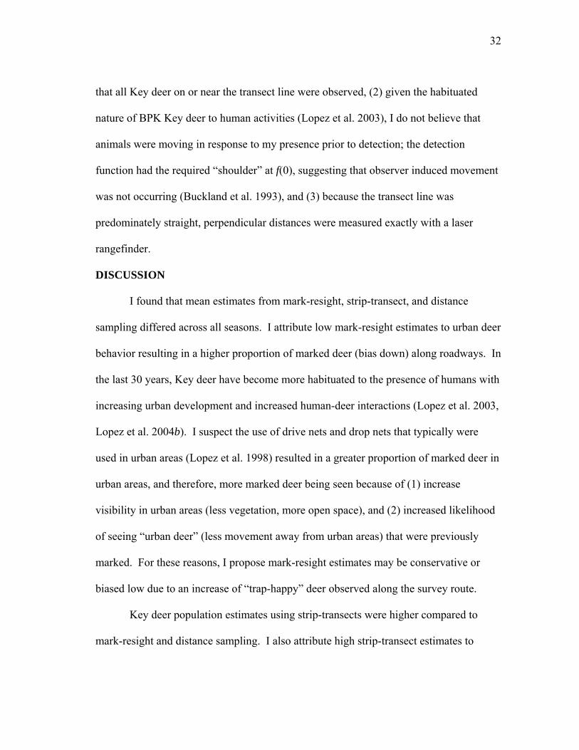
I found mark-resight estimates were lower ( x = 384, 95% CI = 346–421)
strip-transect estimates (
than
x = 854, 95% CI = 806–902) and distance estimates ( x =
95% CI = 488–557, Fig. 3.4). In combining all 3 method estimates, overall popul
mean (
523,
ation
x = 587, 95% CI = 555–619) was similar to the distance estimates. The AN
results for between-subject effects (i.e., method) revealed a significant difference
between the 3 methods (P < 0.001), and significant method × season interactions (P <
0.001) (Fig. 3.3). Post-hoc tests indicated that all methods were significantly differen
and that estimates from the spring (fawning) season were significantly different from the
winter (pre-fawning season, Fig. 3.4). The best model (by AIC selection; AIC = 8,335)
for estimating Key deer density with Program DISTANCE was the hazard model with
no adjustment terms obtained as a global detection function using data from all str
(i.e., surveys, n = 100).
For my study, encounter rate, cluster size, and density were es
OVA
t,
ata
timated by
a pooled estimate of density made from stratum estimates treated as
litated my intent to compare point estimates between methods while
l
ring
stratum, with
replicates. This faci
accounting for the behavioral changes that occur seasonally. Assessing the validity of
the 3 underlying assumptions was not as difficult in my study: (1) transect was a wel
traveled road with good visibility on the adjacent right of way on either side, ensu
30
for Florida Key deer, July 2003-May 2004.
2
2.5
Winter Spring Summer Fall
Season
3
3.5
Y1)
Log
(+
DistanceStrip-transectMark-resight
Figure 3.3. Estimated marginal means (Log[Y+1] transformed) by method and season
2.5
3
3.5
Log
(Y+1
)
WinterSpringSummerFall
2Distance Strip-
TransectMark-
Resight
31
0
200
400
600
800
1000
1200
Winter Spring Summer Fall
Mark-resightStrip-transectDistance
Popu
latio
n E
stim
ate
Figure 3.4. Florida Key deer density estimates ( x , 1 SE) by season and method (mark-
sight, strip-transect, and distance) for Big Pine Key, Monroe County, Florida, July 003
re2
32
that all Key deer on or near the transect line were observed, (2) given the habituated
nimals were moving in response to my presence prior to detection; the detection
nction had the required “shoulder” at f(0), suggesting that observer induced movement
not occurring (Buckland et al. 1993), and (3) because the transect line was
ominately straight, perpendicular distances were measured exactly with a laser
efinder.
CUSSION
I found that mean estimates from mark-resight, strip-transect, and distance
ampling differed across all seasons. I attribute low mark-resight estimates to urban deer
ehavior resulting in a higher proportion of marked deer (bias down) along roadways. In
e last 30 years, Key deer have become more habituated to the presence of humans with
creasing urban development and increased human-deer interactions (Lopez et al. 2003,
n urban areas (Lopez et al. 1998) resulted in a greater proportion of marked deer in
urban areas, and therefore, more marked deer being seen because of (1) increase
visibility in urban areas (less vegetation, more open space), and (2) increased likelihood
of seeing “urban deer” (less movement away from urban areas) that were previously
marked. For these reasons, I propose mark-resight estimates may be conservative or
biased low due to an increase of “trap-happy” deer observed along the survey route.
Key deer population estimates using strip-transects were higher compared to
mark-resight and distance sampling. I also attribute high strip-transect estimates to
nature of BPK Key deer to human activities (Lopez et al. 2003), I do not believe that
a
fu
was
red
ang
IS
p
r
D
s
b
th
in
Lopez et al. 2004b). I suspect the use of drive ne and drop nets that typically were
used i
ts
33
urban deer behavior along roadways, and in addition, a reduced effective strip width
(ESW) along the survey route. First, the strip-transect estimate may be biased high
because surveys were conducted along roadways where Key deer are easily seen o
to frequent (Lopez et al. 2003), resulting in a likely overestimation (Thompson et al.
1998, Pierce and Baccus 1999, Pierce 2000). A second factor may be the dense
vegetation on BPK. The semi-deciduous vegetation in the Lower Florida Keys is
primarily of W
r tend
est Indian origin with limited visibility (Folk 1991). I suspect the
rom monthly maximum sighting distances for the strip-transects (perceived ESW f x =
7 m) w stance 2 as underestimated, whereas use of actual animal sighting distances from di
sampling (ESW x = 38 m) was larger resulting in a larger area sampled. For these
reasons, I suspect use of strip-transects in my study inflated the overall Key deer
population estimate. Burnham et al. (1985) found similar results in their study of
efficiency and bias in transect sampling.
Assuming the combined sum of all 3 methods captures the true population mean
( x = 587, 95% CI = 555–619), I propose that distance sampling may be a more accurate
and reliable means of estimating Key deer density. In addition to my distance est
being similar to the overall grand mean (523 versus 534), this estimate also is similar to
the estimate reported by Lopez et al. (2004a, 523 versus 406). One advantage of
distance sampling is the previously mentioned biases for the other methods (i.e., urban
deer behavior of marked deer, vegetation density, etc.) may not have a strong influence
imate
the d ng in istance estimate. For example, the spatial distribution of the target animals alo
the survey does not have to be uniform in order to obtain a reliable population estimate

34
from distance methods (Buckland et al. 1993, Tomas et al. 2001, Forcardi et al. 2002b
Koenen et al. 2002), which is problematic with mark-resight and strip-transect estim
Vegetation characteristics also influence the ESW in obtaining density estimates,
particularly with strip-transect estimates (Burnham et al. 1985). As previously
mentioned, these biases are likely reduced in distance sampling.
MANAGEMENT IMPLICATIONS
I recommend the use of distance sampling for future monitoring of the Ke
population on BPK. Since 1968, USFWS biologists have collected population tren da
for Key deer (Lopez et al. 2004a); I proposed modifications to data collected along this
route could yield population density estimates that would be beneficial in the monito
of this endangered population. Study results suggest that density estimates were
accurate, precise, easily obtained by field personnel, and therefore, more cost-effec
Similar modifications to survey methods co
,
ates.
y deer
ta
ring
tive.
mmonly used by white-tailed deer managers
could a
d
fford better estimates that are accurate and precise at a low cost.
35
CHAPTER IV
SUMMARY AND SURVEY RECOMMENDATIONS FOR ESTIMATING KEY
DEER DENSITY
The purpose of this chapter is to summarize methods used to estimate Fl
Key deer densities within the National Key Deer Refuge. This ch
orida
apter also will provide
s to U. S. Fish and Wildlife Service (USFWS)
biologi
d” is a
many wildlife management endeavors (Leopold 1933). In the case of
e Key deer, population density/trend estimates are important for developing proper
conservation policy and management protocols (Gelatt and Siniff 1999, Koenen et al.
2002, Swann et al. 2002), and is mandated in the current Key Deer Recovery Plan (U. S.
Fish and Wildlife Service [USFWS] 1999). As a point of departure, I will define 2 terms
that often are used interchangeably in wildlife population estimation but that differ in
meaning. Population density refers to the number of animals per unit area, and answers
the question “how many?” (Krebs 1999). Conversely, population trends or trend
official recommendations and guideline
sts in future efforts to monitor population numbers for the endangered Key deer.
The chapter is divided into 2 parts: (1) a review of past efforts to estimate Key deer
density or monitor population trends, and (2) recommendations and guidelines for future
monitoring of the Key deer population. These recommendations will be based on
findings in previous chapters (Chapters II-III).
HISTORICAL SURVEYS
Reliable population estimates are paramount in the field of wildlife ecology
(Jenkins and Marchinton 1969) because assessment of “the stock on han
prerequisite for
th
36
estimates refers to a relative index to population density (Krebs 1999). Trend data
s
spotlight counts). For example, the deer seen on a spotlight count is
) and No Name (NNK) keys using
y 1975, Lopez 2001) and distance sampling techniques
er)
K=76)
y
-
imply shows variation in the population between sampling periods (e.g., year-to-year
average number of
not an estimate of deer density because it is unlikely that all deer were counted. The
usefulness of trend estimates is tracking changes in population density, assuming
methods used between sampling periods are identical (Krebs 1999). For management
purposes, trend estimates are often useful indices in comparison to population density
estimates due to their ease in implementation.
In reviewing population counts for Key deer, both population density and trend
estimates have been collected since 1968 (Lopez et al. 2004a). Population density
estimates have been conducted on Big Pine (BPK
mark-resight procedures (Silv
(Chapter III). The first density estimate was obtained in 1971-1972 for BPK (167 de
and NNK (34 deer, Silvy 1975). A more recent density estimate (BPK=406, NN
was obtained in 1998-2001 (Lopez 2001) using methods identical to Silvy (1975). Silv
(1975) and Lopez (2001) used the same survey route on BPK (hereafter known as the
BPK 44-mile, BPK 10-mile, Fig. 4.1) in obtaining their estimates (Table 4). Survey
estimates were conducted at sunrise and 1.5 hours before sunset (Lopez 2001).
Since 1975, USFWS biologists have collected population trend data for the Key
deer population via night spotlight counts on a modified version of the original BPK 44
mile route (Silvy 1975, Lopez 2001). The USFWS route (also known as the FWS Fall
37
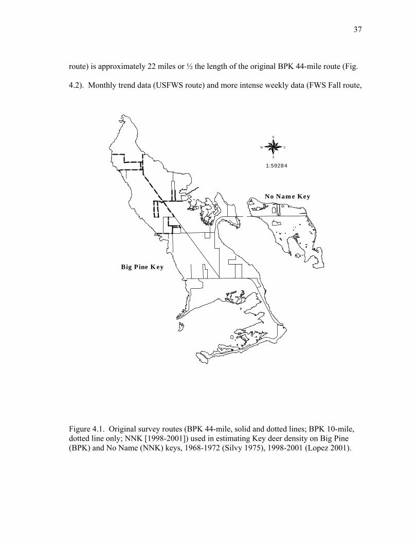
route) is approximately 22 miles or ½ the length of the original BPK 44-mile route (
4.2). Monthly trend data (USFWS route) and more intense weekly data (FWS Fall rout
Fig.
e,
N
EW
S
1:59284
No Nam e Key
Big Pine K ey
Figure 4.1. Original survey routes (BPK 44-mile, solid and dotted lines; BPK 10-mile, dotted line only; NNK [1998-2001]) used in estimating Key deer density on Big Pine (BPK) and No Name (NNK) keys, 1968-1972 (Silvy 1975), 1998-2001 (Lopez 2001).

38
No Name Key
Big Pine Key
N
EW
S
1:49162
Figure 4.2. Official U. S. Fish and Wildlife Service (USFWS) survey route used in monitoring Key deer population trends on Big Pine (BPK) and No Name (NNK) keys,1975-present.
39
5-7 times/week, first week of October) have been collected by USFWS biologists
between 1975-present during evening hours (Fig. 4.2, Table 4.1, Lopez 2001). The FWS
Fall surveys were initiated in 1988 to collect reproductive data (e.g., fawns/doe). In
2002, the USFWS route was slightly modified to include roads from both survey routes
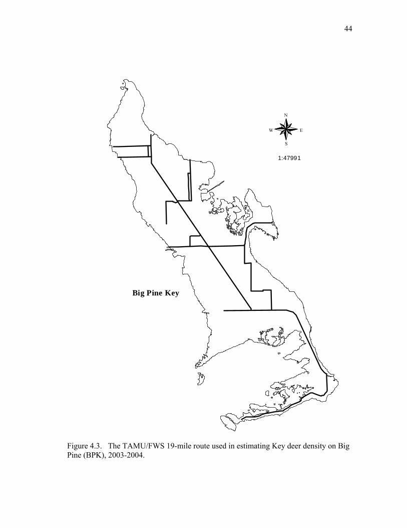
where frequent deer observations were recorded (hereafter TAMU/FWS route, Fig. 4.3).
Mark-resight and distance sampling procedures were used in estimating Key deer
densities using this modified route (Chapter III). Using this modified route, 508 deer
were estimated on BPK using distance methods (Chapter III).
Previous efforts to estimate deer densities on outer islands (defined here as islands
in Key deer range excluding BPK and NNK) have been restricted due to accessibility
issues and/or low deer densities. In most cases, traditional road survey techniques
cannot be implemented for the majority of the islands due to the absence of roads (only
40% [9/20] of islands occupied by Key deer have roads). Future research evaluating
reliable methods to estimate Key deer densities on outer keys is needed. In comparing
the application of infrared-triggered camera (ITC) estimates to road counts, similar
results suggest ITC estimates can be useful in this effort (Chapter II).
SURVEY RECOMMENDATIONS
Based on my review of previous methods to survey Key deer density/trends, I
would recommend (1) continued monitoring of Key deer population trends via mont
spotlight surveys, (2) estimating population density for BPK and NNK using a distance
hly
sampling twice a year (October and April, 5-7 surveys 1st week of month), and (3)
40
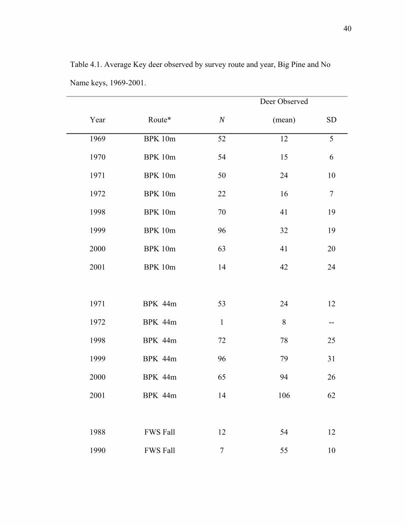
Table 4.1. Average Key deer observed by survey route and year, Big Pine and No
Name keys, 1969-2001.
Year Route* N
Deer Observed
(mean) SD
1969 BPK 10m 52 12 5
1970 BPK 10m 54 15 6
1971 BPK 10m 50 24 1
1972 BPK 10m 22 16 7
1998 BPK 10m 70
0
41 19
31
65 94 26
1999 BPK 10m 96 32 19
2000 BPK 10m 63 41 20
2001 BPK 10m 14 42 24
1971 BPK 44m 53 24 12
1972 BPK 44m 1 8 --
1998 BPK 44m 72 78 25
1999 BPK 44m 96 79
2000 BPK 44m
2001 BPK 44m 14 106 62
1988 FWS Fall 12 54 12
1990 FWS Fall 7 55 10
41
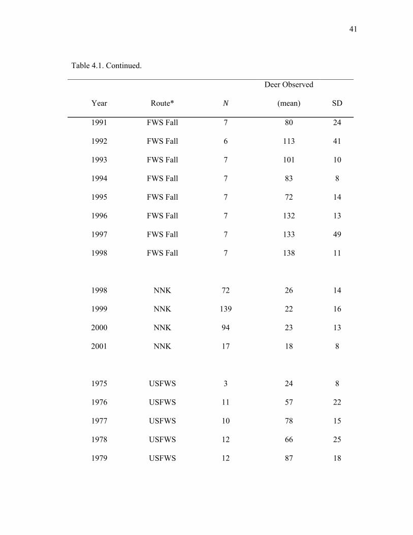
Table 4.1. Continued.
Year Route* N
Deer Observed
SD (mean)
1991 F WS Fall 7 80 24
1992 FWS Fall 6 113 41
1993 FWS Fall 7 101 10
1994 FWS Fall 7 83 8
1995 FWS Fall 7 72 14
1996 FWS Fall 7 132 13
1997 FWS Fall 7 133 49
1998 FWS Fall 7 138 11
1998 NNK 72 2 14
1977 USFWS 10 78 15
6
1999 NNK 139 22 16
2000 NNK 94 23 13
2001 NNK 17 18 8
1975 USFWS 3 24 8
1976 USFWS 11 57 22
1978 USFWS 12 66 25
1979 USFWS 12 87 18
42
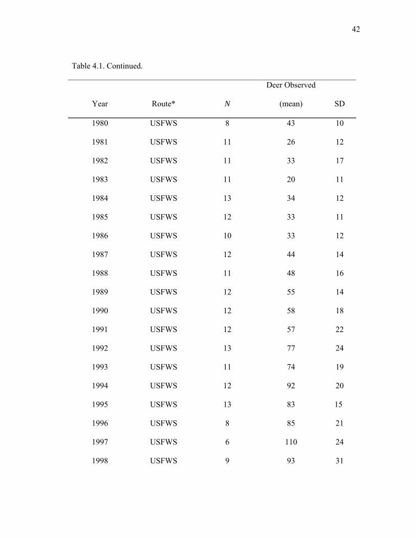
Table 4.1. Continued.
Year Route* N
Deer Observed
(mean) SD
1980 USFWS 8 43 10
1981 USFWS 11 26 12
1982 USFWS 11 33 17
1983 USFWS 11 20 11
1984 USFWS 13 34 12
1985 USFWS 12 33 11
1986 USFWS 10 33 12
1987 USFWS 12 44 14
1988 USFWS 11 48 16
U
U
U
U
1993 USFWS 11 74 19
1989 SFWS 12 55 14
1990 SFWS 12 58 18
1991 SFWS 12 57 22
1992 SFWS 13 77 24
1994 USFWS 12 92 20
1995 USFWS 13 83 15
1996 USFWS 8 85 21
1997 USFWS 6 110 24
1998 USFWS 9 93 31
43
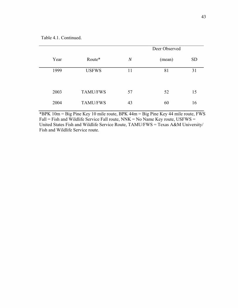
Table 4.1. Continued.
Year Route* N
Deer Observed
(mean) SD
1999 USFWS 11 81 31
2003 TA S
TA S
MU/FW 57 52 15
2004 MU/FW 43 60 16
*BPK 10m = Big Pine K e route, BPK = Big Pine Key 44 mile route, FWS Fall = Fish and Wildlife Service Fall route, NNK = No Name Key route, USFWS = United Fish and W rvice Route, TAMU/FWS = Tex &M Univ y/ Fish and Wildlife Service route.
ey 10 mil 44m
States ildlife Se as A ersit
44
Big Pine Key
1 1:4799
N
EW
Figure 4.3. The TAMU/FWS 19-mile route used in estimating Key deer density on Big Pine (BPK), 2003-2004.
S
45
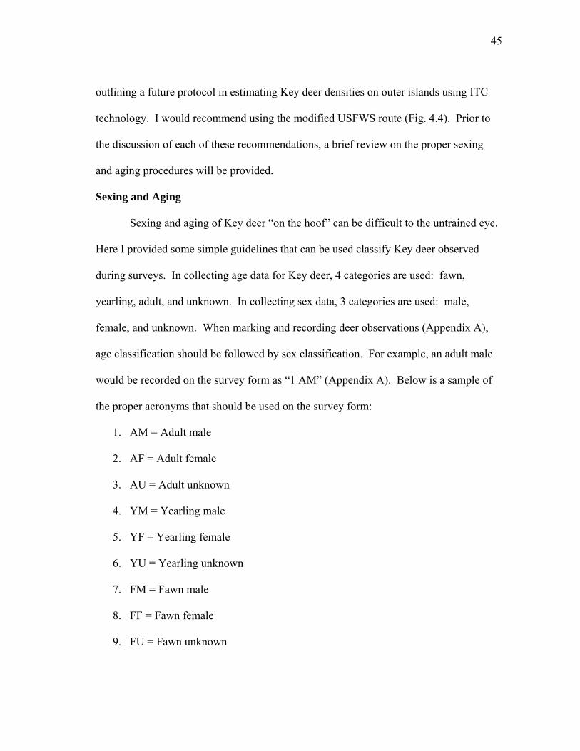
outlining a future protocol in estimating Key deer densities on outer islands using ITC
technology. I would recommend using the modified USFWS route (Fig. 4.4). Prior to
the discussion of each of these recommendations, a brief review on the proper sexing
and aging procedures will be provided.
Sexing and Aging
Sexing and aging of Key deer “on the hoof” can be difficult to the untrained eye.
Here I provided some simple guidelines that can be used classify Key deer observed
during surveys. In collecting age data for Key deer, 4 categories are used: fawn,
yearling, adult, and unknown. In collecting sex data, 3 categories are used: male,
female, and unknown. When marking and recording deer observations (Appendix A),
age classification should be followed by sex classification. For example, an adult male
would be recorded on the survey form as “1 AM” (Appendix A). Below is a sample of
the proper acronyms that should be used on the survey form:
1. AM = Adult male
2. AF = Adult female
3. AU = Adult unknown
4. YM = Yearling male
5. YF = Yearling female
6. YU = Yearling unknown
7. FM = Fawn male
8. FF = Fawn female
9. FU = Fawn unknown
46
N
EW
S
Big Pine Key
Figure 4.4. Proposed survey route for future Key deer monitoring by the U. S. Fish and Wildlife Service (USFWS). Survey route is slightly modified from the official USFWS rou for recent road closures and high density developments. Arrows indicate the direction of travel (no double counting).
1:51683
No Name Key
te (Figure 4.2), accounting

47
10. UM = Unknown male
11. UF = Unknown female
12. UU = Unknown Unknown
It is important to record age followed by sex, otherwise misclassifications can occur.
For example, a “FU” could be “female unknown” if sex and age are reversed (a simple
mnemonic is “Remember your ASS” – Age, Sex, Stupid).
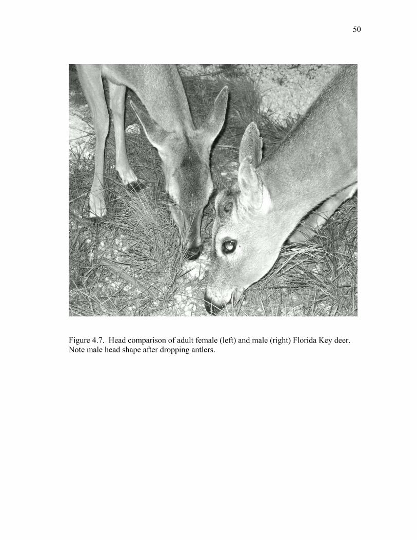
Sexing.—Sexing Key deer becomes easier with increasing age. For the majority
of the year, males have antlers which quickly serve to separate them from females (Figs.
4.5-4.7). When male Key deer have dropped their antlers, their heads tend to be flat or
blocking as compared to the rounded head of females (Fig. 4.7). Male heads can be
considered to be like Frankenstein versus females which resemble the Pope’s round
skullcap (i.e., zucchetto) (Fig. 4.7). Correctly classifying the sex of observed Key deer
becomes more difficult in younger age classes. For spotted fawns (< 6 months of age),
sex determination is difficult in the field and should be avoid. Instead, spotted fawns
should be classified as “fawn unknown”.
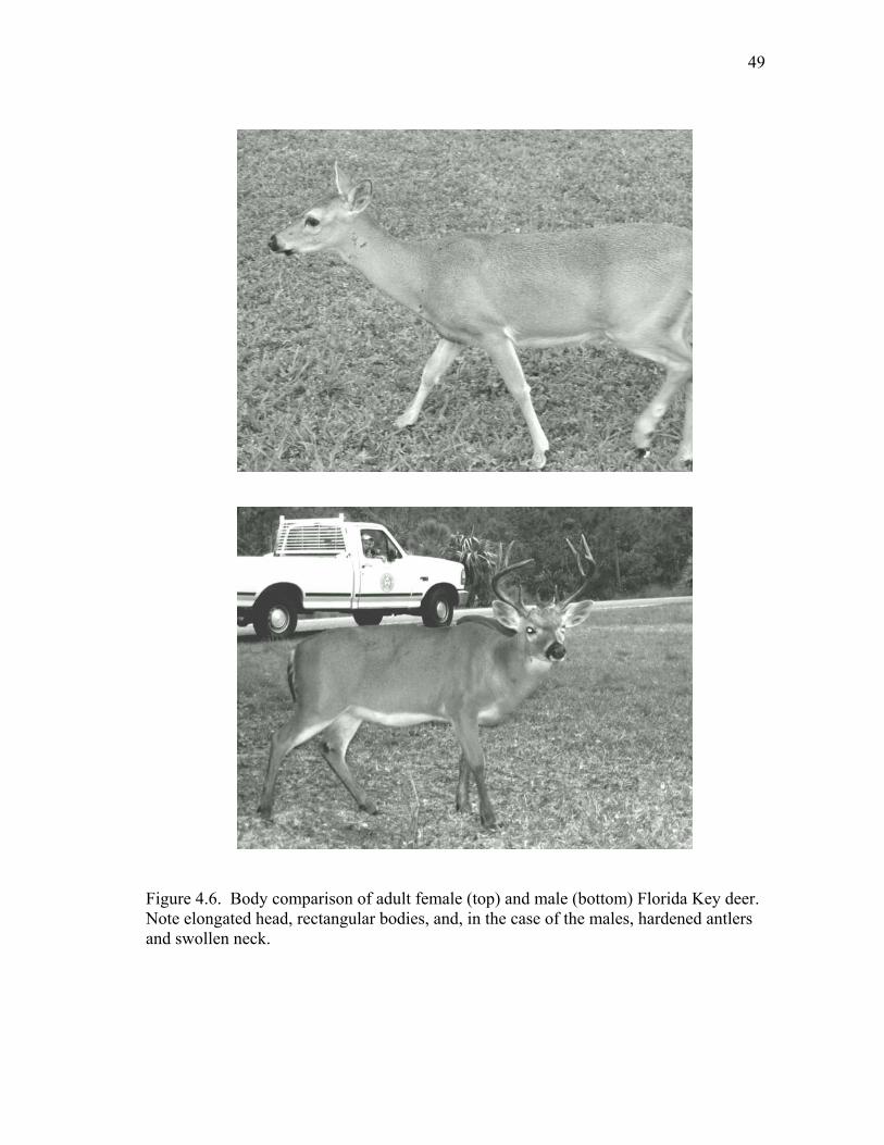
Aging.—Body size and head shape are 2 common traits that can be used in
determining the age class of Key deer. Fawns and yearlings tend to have “square” or
“blocked” body sizes whereas adults tend to be more rectangular and elongated (Fig.
4.5). For males, “buttons” or “spikes” are typically younger age-classes (Fig. 4.5).
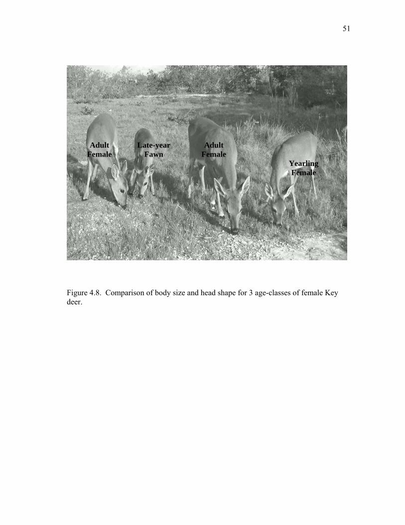
Head shape between adults, yearlings, and fawns can be compared to the relative size of
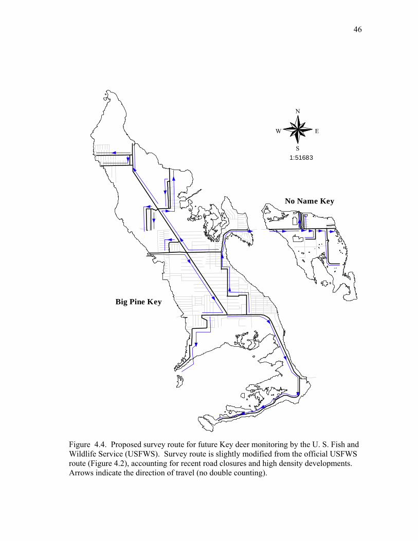
egg plants, papayas, and mangos, respectively (Fig. 4.8).
48
Figure 4.5. Relative size comparison of Flovary between adults (size of egg plant), yea
rida Key deer by sex and age. Head shapes rlings (size of papaya), and fawns (size of
mango).
Adult Male
Adult Female
Yearling Female
Yearling Male Fawn Male Fawn Female
49
Figure 4.6. Body comparison of adult female (top) and male (bottom) Florida Key deer. Note elongated head, rectangular bodies, and, in the case of the males, hardened antlers and swollen neck.
50
Figure 4.7.
ote male head shape after dropping antlers. Head comparison of adult female (left) and male (right) Florida Key deer.
N
51
Adult Female
Late-year Fawn
Adult Female
Yearling Female
Figure 4.8. Comparison of body size and head shape for 3 age-classes of female Key deer.

52
Population Trends (Monthly Surveys)
Key deer population trend data have been collected by USFWS personnel since
1975. The continuation of monthly Key deer spotlight counts is recommended in
maintaining this long-term data set. At the beginning of each month, the new proposed
USFWS route (Fig. 4.4) should be driven with 2 observers recording the sex, age,
location, and marker number (if animal is ith collar). The survey route should
be conducted 1 hour after official sunset in a vehicle traveling 10–15 m 4 km/h).
Two hand-held spotlights (approximately 100,000 candlepower) and the appropriate
forms (Appendix A) should be used in recording Key deer observations. Key deer
should not be counted on portions of the survey route that have been previously driven
(no double counting). The expected drive time for the survey route is approximately
opulation Density (Biannual Surveys)
Key deer population density estimates were conducted in 1968-1972 (Silvy
1975), 1998-2001 (Lopez 2001), and 2003-2004 (Chapter III). Distance sampling
surveys should be conducted 2 times annually the first week of April (spring survey
during fawning season) and October (fall survey during breeding season) using the new
proposed USFWS route (Fig. 4.4). Similar to the trend surveys, the route should be
driven with 2 observers recording the sex, age, location, marker number (if animal is
marked with collar), and deer distance from vehicle (Appendix A). Distance should be
obtained using laser range finders (Chapter III). The survey route should be conducted
1.5 hours prior to official sunset in a vehicle traveling 16–37 mph (25–60 km/h).
marked w
ph (16–2
2.5–3 hours. All data should be summarized and entered into the Access database.
P
53
Observed Key deer should not be double counted on portions of the survey route that
97).
have been previously driven. The expected drive time for the survey route is
approximately 2–2.5 hours. All data should be summarized and entered in Access
database and Arcview GIS for further analysis (Lopez 2001). Distance data can be
analyzed using Program DISTANCE (Buckland et al. 1993, Focardi et al. 2002a).
Outer Key Estimates
Use of ITC in estimating Key deer density is promising for outer island estimates
(Chapter II). Infrared-triggered cameras can provide wildlife managers with density
estimates and information on herd composition (Mace et al. 1994, Jacobson et al. 19
The use of ITC may not be practical for large areas; however, their use may be cost-
effective, particularly in areas where habitat and/or lack of infrastructure (i.e., roads)
preclude the use of other methods. Continued research with ITC use is needed.
54
LITERATURE CITED
Anderson, D. R. 2001. The need to get the basics right in wildlife field studies. Wildlife
Society Bulletin 29:1294–1297.
_____. 2003. Response to Engeman: index values rarely constitute reliable information.
Wildlife Society Bulletin 31:288–291.
_____, J. L. Laake, B. R. Crain, and K. P. Burnham. 1979. Guidelines for line transect
sampling of biological populations. Journal of Wildlife Management 43:70-78.
Bear, G. D, G. C. White, L. H. Carpenter, R. B. Gill, and D. J. Essex. 1989. Evaluation
of aerial mark-resighting estimates of elk populations. Journal of Wildlife
Management 53:908–915.
Beechinor, D. B. 1986. Preburn and postburn activity patterns of white-tailed deer
(Odocoileus virginianus). Thesis. Southwest Texas State University, San Marcos,
Texas, USA.
ender, L. C., W. L. Meyers, and W. R. Gould. 2003. Comparison of helicopter and
ground surveys for North American elk Cervus elaphus and mule deer
Odocoileus hemionus population composition. Wildlife Biology 9:199–205.
uckland, S. T., D. R. Anderson, K. P. Burnham, and J. L. Laake. 1993. Distance
sampling. Estimating abundance of biological populations. Chapman & Hall,
London, reprinted 1999 by RUWPA, University of St. Andrews, Scotland.
446pp.
rnham, K. P. and D. R. Anderson. 1984. The need for distance data in transect
counts. Journal of Wildlife Management 48:1248–1254.
B
B
Bu

55
_____, _____, and J. L. Laake. 1985. Efficiency and bias in strip and line transect
sampling. Journal of Wildlife Management 49:1012–1018.
Carthew, S. M., and E. Slater. 1991. Monitoring animal activity with automated
photography. Journal of Wildlife Management 55:689–692.
Corn, J. L. and M. J. Conroy. 1998. Estimation of density of mongooses with capture-
recapture and distance sampling. Journal of Mammalogy 79:1009–1015.
Cypher, B. L. 1991. A technique to improve spotlight observations of deer. Wildlife
Society Bulletin 19:391–393.
Dickson, J. D., III. 1955. An ecological study of the Key Deer. Florida Game and
Fresh Water Fish Commission Technical Bulletin 3, Tallahassee, Florida, USA.
Ellingson, A. R., and P. M. Lukacs. 2003. Improving methods for regional landbird
monitoring: a reply to Hutto and Young. Wildlife Society Bulletin 31:896–902.
Folk, M. L. 1991. Habitat of the Key deer. Dissertation, Southern Illinois University,
Carbondale, Illinois, USA.
Forcardi, S., R. Isotti, E. R. Pelliccioni, and D. Iannuzzo. 2002a. The use of distance
sampling and mark-resight to estimate the local density of wildlife populations.
Environmetrics 13:177–186.
_____ , _____ , and A. Tinelli. 2002b. Line transect estimates of ungulate populations
in a Mediterranean forest. Journal of Wildlife Management 66:48–58.
Foster, M. L., and S. R. Humphrey. 1995. Use of highway underpasses by Florida
panthers and other wildlife. Wildlife Society Bulletin 23:95–100.
56
Geisser, S., and S. W. Greenhouse. 1958. An extension of Box's results on the use of
F distribution in multivariate analysis. Annals of Mathematic
the
al Statistics 29:885–
Gelatt, ter seals in the
Gill, R
6.
in
Heilbru
Hirst, S. M. 1969. Road-strip census techniques for wild ungulates in African woodland.
Huynh grees of
891.
T. S., and D. B. Siniff. 1999. Line transect survey of crabea
Amundsen-Bellingshausen Seas, 1994. Wildlife Society Bulletin 27:330–336.
. M. A., M. L. Thomas, and D. Stocker. 1997. The use of portable thermal
imaging for estimating deer population density in forest habitats. Journal of
Applied Ecology 34:1273–128
Hardin, J. W., W. D. Klimstra, and N. J. Silvy. 1984. Florida Keys. Pages 381–390
L. K. Halls, editor. White-tailed deer: ecology and management. Stackpole
Books, Harrisburg, Pennsylvania, USA.
n, R. D., N. J. Silvy, M. E. Tewes, and M. J. Peterson. 2003. Using automatically
triggered cameras to individually identify bobcats. Wildlife Society Bulletin
31:748–755.
Hiby, L. and M. B. Krishna. 2001. Line transect sampling from a curving path.
Biometrics 57:727–731.
Journal of Wildlife Management 33:40–48.
, H., and L. S. Feldt. 1976. Estimation of the Box correction factor for de
freedom from sample data in the randomized block and split-plot designs.
Journal of Educational Statistics 1:69-82.
57
Jachmann, H. 2002. Comparison of aerial counts with ground counts for large African
herbivores. Journal of Applied Ecology 39:841–852.
Jacobson, H. A., J. C. Kroll, R. W. Browning, B. H. Koerth, and M. H. Conway. 1997.
rn
mposium. U.S. Forest Service, Southern
Johnso ic
ometrics 41:669–679.
_____, and J. K. Nichols. 1998. Estimation of tiger densities in India using photographic
Koenen and P. R. Krausman. 2002. Using distance sampling to
Krebs, ond edition. Addison-Wesley
Publishers, Menlo Park, California, USA.
Infrared-triggered cameras for censusing white-tailed deer. Wildlife Society
Bulletin 25:547–556.
Jenkins, J. H., and R. K. Marchington. 1969. Problems in censusing the white-tailed
deer. Pages 115–118 in L. K. Halls, editor. White-tailed deer in the southeaste
forest habitat: proceedings of a sy
Forestry Experiment Station, New Orleans, Louisiana, USA.
n, E. G. and R. D. Routledge. 1985. The line transect method: a nonparametr
estimator based on shape restrictions. Bi
Karanth, K.U. 1995. Estimating tiger populations from camera-trap data using capture-
recapture models. Biological Conservation 71:333–338.
captures and recaptures. Ecology 79:2852–2862.
, K. K. G., S. DeStefano,
estimate seasonal densities of desert mule deer in a semidesert grassland.
Wildlife Society Bulletin 30:53–63.
Koerth, B. H., and J. C. Kroll. 2000. Bait type and timing for deer counts using cameras
triggered by infrared monitors. Wildlife Society Bulletin 28:630–635.
C. J. 1999. Ecological methodology. Sec
58
Kucera, T. E., A. M. Soukkala, and W. J. Zielinski. 1995. American marten, fisher, lynx,
and wolverine: survey methods for their detection. US
DA Forest Service General
Lancia
ulations. Pages 215–253 in T. A. Bookhout, editor.
Langdo 1. A
s in West Virginia.
Leopol ork, New York,
Lomax education and
_____, N. J. Silvy, P. A. Frank, and B. L. Pierce. 2003a. Effects of supplemental
_____, e Key
Technical Report PSW GTR-157.
, R. A., J. D. Nichols, and K. H. Pollack. 1994. Estimating the number of
animals In wildlife pop
Research and management techniques for wildlife and habitats. Fifth edition.
The Wildlife Society, Washington, D.C., USA.
n, C. A., J. T. Anderson, J. M. Crum, W. M. Ford, and J. W. Edwards. 200
comparison of white-tailed deer population estimation method
Thesis, West Virginia University, Morgantown, West Virginia, USA.
d, A. 1933. Game management. Charles Scribner's Sons, New Y
USA.
, R. G. 2001. Statistical concepts: a second course for the
behavioural sciences. Second edition. Lawrence Erlbaum Associates, Mahwah,
New Jersey, USA.
Lopez, R. R. 2001. Population ecology of Florida Key deer. Dissertation, Texas A&M
University, College Station, Texas, USA.
feeding of Key deer behavior in urban areas. Florida Scientist. 66:267-272.
_____, R. F. Labisky, and P. A. Frank. 2003b. Hurricane impacts on th
deer in the Florida Keys. Journal of Wildlife Management 67:280–288.
59
_____, _____, B. L. Pierce, P. A. Frank, M. T. Wilson, and K. M. Burke. 2004a.
Population density of the endangered Florida Key deer. Journal of Wildlife
Management 68:570–575.
_____, _____, J. D. Sebesta, S. D. Higgs, and M. Salazar. 1998. A portable drop n
capturing urban deer. Proceedings of the Southeastern Association of Fish an
Wildlife Agencies 52:206–209.
_____, R. N. Wilkins, P. A. Frank, M. J. Peterso
et for
d
_____, n, and N. M. Peterson. 2004b.
_____, s. 2003c.
ement 67:34–45.
zly bear
Mackenzie, D. I., and W. L. Kendall. 2002. How should detection probability be
Mason, J. R., N. J. Bean, and L. Clark. 1993. Development of chemosensory attractants
.
McCul
_____. al of
Wildlife Management 46:963–973.
Habitat use patterns of Florida Key deer: Implications of urban development.
Journal of Wildlife Management 68:900–908.
M. E. Viera, N. J. Silvy, P. A. Frank, S. W. Whisenant, and D. A. Jone
Survival, mortality, and life expectancy of Florida Key deer. Journal of Wildlife
Manag
Mace, R. D., S. C. Minta, T. L. Manley, and K. E. Aune. 1994. Estimating griz
population size using camera sightings. Wildlife Society Bulletin 22:74–83.
incorporated into estimates of relative abundance? Ecology 83:2387–2393.
for white-tailed deer (Odocoileus virginianus). Crop Protection 12:448–452
lough, D. R. 1979. The George Reserve deer herd: Population ecology of a K
selected species. University of Michigan Press, Ann Arbor, Michigan, USA.
1982. Evaluation of night spotlighting as a deer study technique. Journ
60
Pierce, B. L. 2000. A non-linear line transect method for estimating white-tailed d
population densities. Thesis, Southwest Texas State University, San Marcos,
Texas, USA.
eer
3. TRC Mariah Associates, Inc., Austin, Texas.
rn Association of Fish and Wildlife Agencies 52:283–
Ransom r in
Savidg
Schaef ve
_____, and J. T. Baccus. 1999. Wildlife trend analysis: A white-tailed deer management
plan for Camp Bullis, Texas. US Army Corps of Engineers Contract DACA63-
92-D-0011, Delivery Order #007
Potvin, F., L. Breton, and L. P. Rivest. 2002. Testing a double-count aerial survey
technique for white-tailed deer, Odocoileus virginianus, in Quebec. Canadian
Field-Naturalist 116:488–496.
Rakestraw, D. L, R. J. Stapper, D. B. Fagre, N. J. Silvy. 1998. A comparison of
precision for three deer survey techniques. Proceedings of the Annual
Conference of Southeaste
293.
, D., Jr., and W. E. Pinchak. 2003. Assessing accuracy of a laser rangefinde
estimating grassland bird density. Wildlife Society Bulletin 31:460–463.
e, J. A., and T. F. Seibert. 1988. An infrared trigger and camera to identify
predators at artificial nests. Journal of Wildlife Management 52:291–294.
er, J., and M. B. Main. 2001. White-tailed deer in Florida. Florida Cooperati
Extension Service, Institute of Food and Agricultural Services, University of
Florida Publication WEC-133.
61
Silvy, N. J. 1975. Population density, movements, and habitat utilization of Key deer,
Odocoileus virginianus clavium. Dissertation, Southern Illinois University,
Carbondale, Illinois, USA.
SPSS.
us
Zoological Society of London 58:131–152.
Swann
n Desert Tortoises. Journal of Wildlife Management 66:969–975.
vidae), population in the Pantanal wetland,
Brazil, using the distance sampling technique. Animal Biodiversity and
Conservation 24:101–106.
_____, J. W. Hardin, and W. D. Klimstra. 1975. Use of a portable net to capture free-
ranging deer. Wildlife Society Bulletin 3:27–29.
2001. SPSS advanced models. Version 11. SPSS, Inc., Chicago, Illinois, USA.
Staines, B. W. and P. R. Ratcliffe. 1987. Estimating the abundance of red deer (Cerv
elaphus L.) and roe deer (Capreolus capreolus L.) and their current status in
Great Britain. Symposia of the
Strandgaard, H. 1967. Reliability of the Peterson Method tested on a roe deer
population. Journal of Wildlife Management 31:643–651.
, D. E., R. C. Averill-Murray, and C. R. Schwalbe. 2002. Distance sampling for
Sonora
Thompson, W. L. 2002. Towards reliable bird surveys: accounting for individuals
present but not detected. Auk 119:18–25.
_____, G. C. White, and C. Gowan. 1998. Monitoring vertebrate populations.
Academic Press, San Diego, California, USA.
Tomas, W. M., W. McShea, G. H. B. de Miranda, J. R. Moreira, G. Mourao, and P. A.
Lima Borges. 2001. A survey of pampas deer, Ozotceras bezoraticus
leucogaster (Arctiodactyla, Cer
62
Tzilkowski, W. M., and G. L. Storm. 1993. Detecting change using repeated measures
analysis: white-tailed deer abundance at Gettysburg National Military Park.
Wildlife Society Bulletin 21:411–414.
, Atlanta, Georgia, USA.
essing
n 22:667–673.
re
opulations. Los Alamos National
Zar, J. rentice Hall, Upper Saddle River,
U.S. Fish and Wildlife Service. 1999. South Florida multi-species recovery plan: Key
deer recovery plan. U.S. Fish and Wildlife Service
von Ende, C. N. 2001. Repeated-measures analysis: growth and other time-dependent
measures. Pages 134–157 in S. M. Scheiner and J. Gurevitch, editors. Design and
analysis of ecological experiments. Oxford University Press, New York, New
York, USA.
Whipple, J. D., D. Rollins, and W. H. Schacht. 1994. A field simulation for ass
accuracy of spotlight deer surveys. Wildlife Society Bulleti
White, G. C., and R. A. Garrott. 1990. Analysis of wildlife radiotracking data.
Academic Press, New York, New York, USA.
White, G. C., D. R. Anderson, K. P. Burnham, and D. L. Otis. 1982. Capture-recaptu
and removal methods for sampling closed p
Laboratory, Los Alamos, New Mexico, USA.
H. 1996. Biostatistical analysis. Third edition. P
New Jersey, USA.

63
APPENDIX A
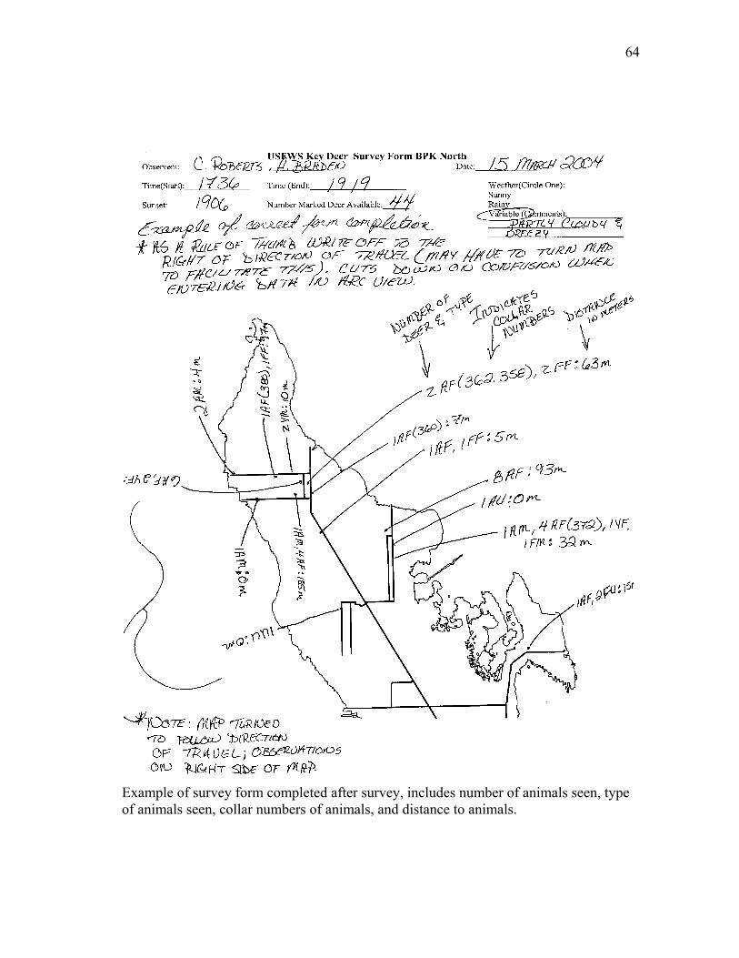
64
Example of survey form completed after survey, includes number of animals seen, type of animals seen, collar numbers of animals, and distance to animals.
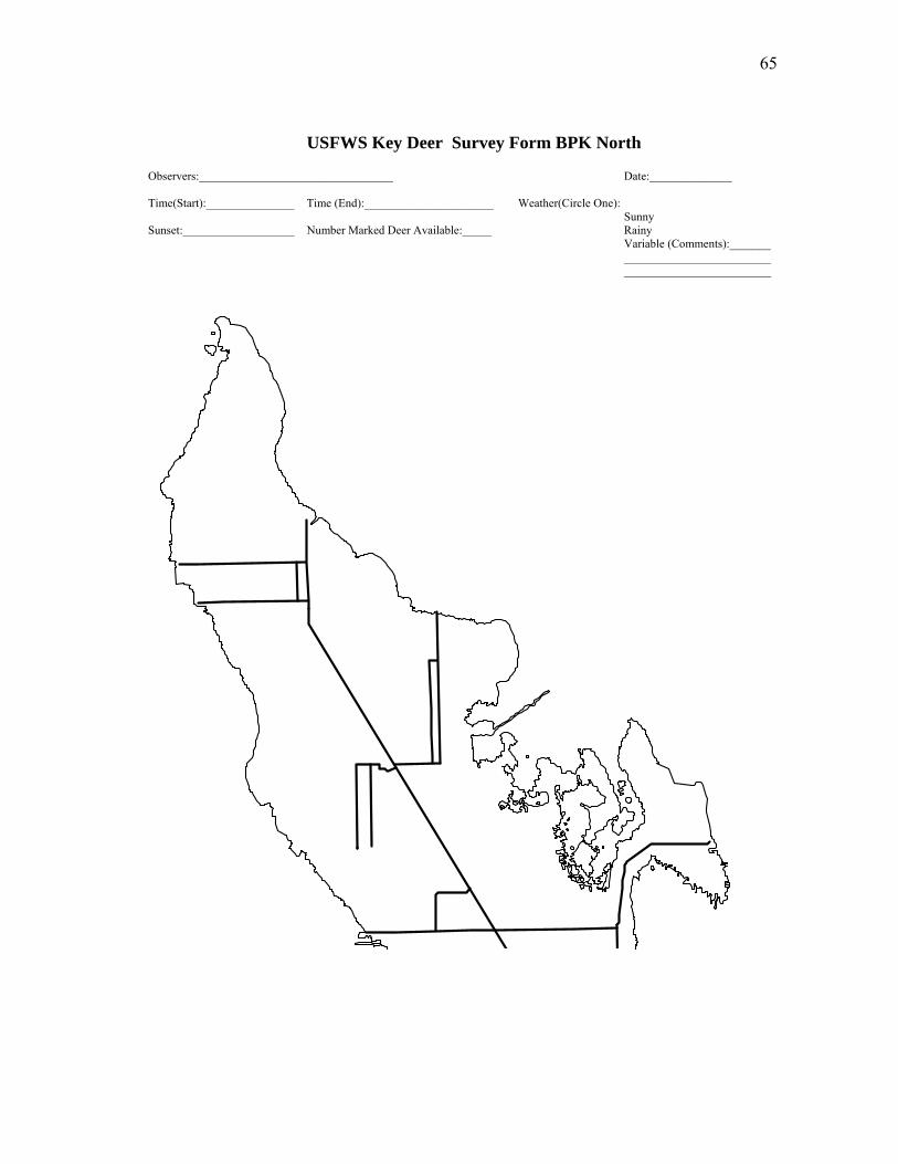
65
USFWS Key Deer Survey Form BPK North
vers:_________________________________ Date:______________
___ ___
Obser Time(Start):_______________ Time (End):______________________ Weather(Circle One): Sunny Sunset:___________________ Number Marked Deer Available:_____ Rainy Variable (Comments):____ ______________________ _________________________
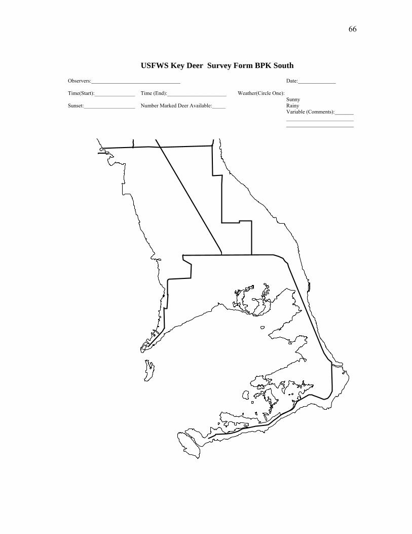
66
USFWS Key Deer Survey Form BPK South
Observers:_________________________________ Date:______________ Time(Start):_______________ Time (End):______________________ Weather(Circle One): Sunny Sunset:___________________ Number Marked Deer Available:_____ Rainy Variable (Comments):_______ _________________________ _________________________

67
USFWS Key Deer Survey Form NNK
Observers:_________________________________ Date:______________ Time(Start):_______________ Time (End):______________________ Weather(Circle One): Sunny Sunset:___________________ Number Marked Deer Available:_____ Rainy Variable (Comments):_______ _________________________ _________________________

68
USFWS Key Deer Summary Tabulation Form
Location AM AF AU YM YF YU FM FF FU UM UF UU
Observers:_________________________________ Date:______________ Time(Start):_______________ Time (End):______________________ Weather(Circle One): Sunny Sunset:___________________ Number Marked Deer Available:_____ Rainy Variable (Comments):_______ _________________________ _________________________
HQ/ Eden Pines
Key Deer Blvd. South
US 1 Business
Palm Villa /Newfound
Harbor
US 1 Undeveloped
Long Beach Rd.
County Rd/Avenue B
Tropical Bay
No Name Key
Key Deer Blvd. North
Koehn’s
Port Pine Heights
Blue Hole/ Pine Heights

69
arents: Nicky and Bill Roberts
Permanent Addre n o D T 6
Born: 11 August 1973, Austin, Texas
EDUC N
Ma e, ildlife and Fisheries Scienc
Bachelor of Science, Wildlife and Fisheries Sciences, Texas A&M University, 1996.
WORK EXPERIE CE
Ranch Hand/ Cow oy, Roberts’ Ranch, Lytton Springs, Texas 1980 - Present.
Research Assistan Departme t of Wildlife and Fisheries Sciences, Texas A&M
University and the National Key Deer Refuge, Big Pine Key, Florida. 200
Teaching Assistan e t of Wildlife and Fisheries Sciences, Texas A&M
rsity, 002 a d 20 4.
Engin echnician, Ducks Unlimited, Inc., Texas Field Office, Richmond,
Airborne Infantryman, United States Army, Fort Bragg, North Carolina 1999 –
Biological Technician, Texas Prairie Wetlands Project, Ducks Unlimited, Inc., osenberg, Texas 1997- 1999.
C
VITA
Clay Walton Roberts
BACKGROUND
P
ss: 722A Old Sa Ant nio Road, ale, exas 7860
ATIO
ster of Scienc W es, Texas A&M University, 2005.
N
b
t, n
t, Departm n
Unive 2 n 0
eering T
2002.
R
B
3-2004
Texas
2002.