PNNL-14891

Estimating Groundwater Concentrations from Mass Releases to the Aquifer at the Integrated Disposal Facility and Tank Farms in the Hanford Central Plateau M. P. Bergeron E. J. Freeman June 2005 Prepared for the U.S. Department of Energy under Contract DE-AC05-76RL01830

DISCLAIMER This report was prepared as an account of work sponsored by an agency of theUnited States Government. Neither the United States Government nor anyagency thereof, nor Battelle Memorial Institute, nor any of their employees,makes any warranty, express or implied, or assumes any legal liability orresponsibility for the accuracy, completeness, or usefulness of anyinformation, apparatus, product, or process disclosed, or represents thatits use would not infringe privately owned rights. Reference herein to any specific commercial product, process, or service by trade name, trademark,manufacturer, or otherwise does not necessarily constitute or imply itsendorsement, recommendation, or favoring by the United States Governmentor any agency thereof, or Battelle Memorial Institute. The views and opinionsof authors expressed herein do not necessarily state or reflect those of theUnited States Government or any agency thereof. PACIFIC NORTHWEST NATIONAL LABORATORY operated by BATTELLE for the UNITED STATES DEPARTMENT OF ENERGY under Contract DE-ACO5-76RLO183O Printed in the United States of America Available to DOE and DOE contractors from the Office of Scientific and Technical Information, P.O. Box 62, Oak Ridge, TN 37831-0062; ph: (865) 576-8401 fax: (865) 576-5728 email: reports@adonis.osti.gov Available to the public from the National Technical Information Service, U.S. Department of Commerce, 5285 Port Royal Rd., Springfield, VA 22161 ph: (800) 553-6847 fax: (703) 605-6900 email: orders@ntis.fedworld.gov online ordering: http://www.ntis.gov/ordering.htm

This document was printed on recycled paper. (8/00)

PNNL-14891

Estimating Groundwater Concentrations from Mass Releases to the Aquifer at the Integrated Disposal Facility and Tank Farms in the Hanford Central Plateau M. P. Bergeron E. J. Freeman June 2005 Prepared for the U.S. Department of Energy under Contract DE-AC05-76RL01830 Pacific Northwest National Laboratory Richland, Washington 99352

iii

Executive Summary

This report summarizes groundwater-related numerical calculations that will support groundwater flow and transport analyses associated with the scheduled 2005 performance assessment of the Integrated Disposal Facility (IDF). The report also provides potential supporting information to other ongoing Hanford Site risk analyses associated with the closure of single-shell tank farms and related actions. The IDF 2005 performance assessment analysis is using well intercept factors (WIFs), as outlined in the 2001 performance assessment of the IDF. The flow and transport analyses applied to these calculations use both a Site-wide regional-scale model and a local-scale model of the area near the IDF. The regional-scale model is used to evaluate flow conditions, groundwater transport, and impacts from the IDF in the central part of the Hanford Site, at the core zone boundary around the 200 East and 200 West Areas, and along the Columbia River. The local-scale model is used to evaluate impacts from transport of contaminants to a hypothetical well 100 m downgradient from the IDF boundary. Analyses similar to the regional-scale analysis of IDF releases are also provided at individual tank farm areas as additional information. The WIF approach for estimating groundwater concentrations involves simulating the groundwater system response from a known concentration of contaminant in water entering the groundwater system from the vadose zone over a water-table surface area that corresponds to the facility footprint. Using this approach, the groundwater system response from a specific mass flux can be simulated independently. The ratio of the estimated concentration in the groundwater to the contaminant concentration at the bottom of the vadose zone can be used to estimate groundwater concentrations at selected locations from mass releases calculated independently from waste release and vadose zone flow and transport to the underlying groundwater system. This approach can be useful in estimating groundwater concentrations at specific locations and can be a desirable alternative when there are more combinations of inventory distri-butions and parameter sets than there are waste form release, vadose zone transport, and groundwater flow and transport scenarios to be simulated. To gain insight on how the WIF approach compares with other approaches for estimating groundwater concentrations from mass releases to the unconfined aquifer, groundwater concentrations were estimated with the WIF approach for two hypothetical release scenarios and compared with similar results using the convolution approach. The convolution approach for estimating groundwater concentrations involves simulating a system response from a unit inventory release through each of the process models (i.e., source release, vadose zone flow and transport, and groundwater flow and transport) and using the results of the calculations with principles of superposition to estimate concentrations in groundwater for a specific constituent inventory distribution. A unit release in each of the process models can be simulated independently. Then, by assuming linearity, the unit release responses from each source area via the process models can be combined or superimposed. One release scenario evaluated with both approaches (WIF and convolution) involved a long-term source release from immobilized low-activity waste glass containing 25,550 Ci of technetium-99 near the IDF (adapted from Mann et al. 2001); another involved a hypothetical shorter-term release of ~0.7 Ci of technetium over 600 years from the S-SX tank farm area, as adapted from Zhang et al. (2004). Direct

iv

simulation results for both of these release scenarios were also provided to compare with WIF and convolution results. For a long-term increasing release of technetium-99 from immobilized low-activity waste (ILAW) glass from the IDF, both methods produced results similar to those from direct simulation, and both methods produced breakthrough curves downgradient from the source area that are similar in shape to the long-term release curve used in the simulation. However, the concentrations estimated by the convolution approach were very like direct simulation results at comparable locations. Predictions using the convolution approach were about 4 percent higher and 10 percent lower than direct simulation predictions at the core zone and along the river, respectively. Results with the WIF approach were similar to those of convolution and direct simulation at the same locations; at the core zone and along the river, WIF results were within 10 percent (higher) and 11 percent (lower), respectively, of direct simulation results. The shorter-term contaminant release scenario simulates a 600-year release of 0.7 Ci of technetium-99 from a hypothetical tank leak in the S-SX tank farm. The convolution approach estimated peak concentrations similar to direct simulation at comparable locations; predictions were about 7 percent higher, 3 percent lower, and 5 percent lower than direct simulation at the 250 m downgradient location, core zone, and river, respectively. The WIF approach produced peak concentrations that were higher at comparable locations than those predicted by convolution and direct simulation. WIF results were most like direct simulation results at the 250 m location, where they were about 50 percent (1.5 times) higher. However, they were much higher at the core zone and along the river—about 17 and 22 times higher, respectively. This analysis concluded that, because the WIF estimation of peak concentration involves scaling the time series of input source concentrations from the vadose zone to the aquifer, results were reasonably accurate for groundwater concentrations near the source. But the convolution approach more closely approximated direct simulation results at locations far from the source. For the two cases considered, the WIF approach overestimated peak concentration locations away from the source area—e.g., at down-gradient locations, as breakthrough curves deviated from the shape of the input function in response to plume dispersion. Results are generally influenced by two factors: 1) the duration of the source term release to the water table and 2) the distance to points of calculation. Comparing WIF results with direct simulation results for the two cases provides a measure of the magnitude of the deviation that could be expected at the core zone and along the river from long- and short-term releases from the IDF in 200 East Area and a tank farm in 200 West Area. Peak concentrations estimated with the WIF approach tend to be closer to results from direct simulation of long-term releases of contaminants from ILAW glass. The breakthrough curves at various points of calculation have shapes similar to the original release curve in the source area. Peak concentra-tions estimated with the WIF approach are higher for short-term releases of contaminants where breakthrough curve shapes at various points of calculation are influenced by plume dispersion and deviate from the original release curve in the source area. For the hypothetical tank leak case evaluated at the S-SX tank farm in the 200 West Area, where the points of calculation are considerably farther from the source, WIF results for the core zone and along the river were on the order of 360 and 210 percent (3.6 and 2.1 times) higher, respectively, than direct simulation results.

v

The Site-wide model used to support these calculations is now being recalibrated to include current data. Many of the calculations in this report will need to be repeated with the recalibrated model when it becomes available later this year. When the updated calculations are completed, this report will be revised and reissued to support ongoing maintenance of the IDF PA. In the interim, the report is being made available electronically to only a limited number of onsite personnel. An electronic version of this report can also be acquired online using the search feature at http://www.pnl.gov/main/publications/. References Bergeron MP and SK Wurstner. 2000. Groundwater Flow and Transport Calculations Supporting the Immobilized Low-Activity Waste Disposal Facility Performance Assessment. PNNL-13400, Pacific Northwest National Laboratory, Richland, Washington.

Mann FM, KC Burgard, WR Root, RJ Puigh, SH Finfrock, R Khaleel, DH Bacon, EJ Freeman, BP McGrail, SK Wurstner, and PE LaMont. 2001. Hanford Immobilized Low-Activity Waste Performance Assessment: 2001 Version. DOE/ORP-2000-24 Rev. 0, U.S. Department of Energy Office of River Protection, Richland, Washington.

Zhang ZF, VL Freedman, SR Waichler, and MD White. 2004. 2004 Initial Assessments of Closure for the S-SX Tank Farm: Numerical Simulations. PNNL-14604, Pacific Northwest National Laboratory, Richland, Washington.

vi

vii

Acronyms and Abbreviations

CFEST Coupled Fluid, Energy, and Solute Transport code

CHARIMA General-purpose computer code for simulating water, sediment, and contaminant movement in channels

GRTPA A computer code that calculates human dose from groundwater

ILAW Immobilized low-activity waste

IDF Integrated Disposal Facility

INTEG Computer program that calculates groundwater contamination and human dose

LLBG Low-level waste burial grounds

RCRA Resource Conservation and Recovery Act

STOMP Subsurface Transport over Multiple Phases (code)

WIF Well intercept factor

viii

ix

Acknowledgments The authors wish to express their thanks to Mark Freshley of PNNL for much appreciated peer review comments and suggestions and to Vicky Freedman and Fred Zhang of PNNL for providing the basic information associated with the shorter-term scenario, a 600-year release of technetium-99 from a hypothetical tank leak in the S-SX tank farm, used in this report. The authors also express their thanks to Doug Hildebrand (DOE-RL) for his ongoing encouragement and support for our efforts and the useful review comments and suggestions he provided on final drafts of the report. We also want to acknowledge the efforts of Sheila Bennett for editorial support and document preparation.

x

xi

Contents Executive Summary ..................................................................................................................................... iii

Acronyms and Abbreviations .....................................................................................................................vii

Acknowledgments........................................................................................................................................ ix

1.0 Introduction ......................................................................................................................................... 1.1 1.1 Background ................................................................................................................................. 1.1

1.1.1 Well Intercept Factor (WIF) Approach................................................................................ 1.1 1.1.2 Convolution Approach ......................................................................................................... 1.3

1.2 Purpose and Scope of Report ...................................................................................................... 1.5

2.0 Conceptual and Numerical Groundwater Model Used in Analyses................................................... 2.1 2.1 Hydrogeologic Framework ......................................................................................................... 2.1

2.1.1 Recharge and Flow System Boundary Conditions............................................................... 2.3 2.1.2 Flow and Transport Properties ............................................................................................. 2.5

2.2 Simulation of Post-Closure Flow Conditions ............................................................................. 2.9

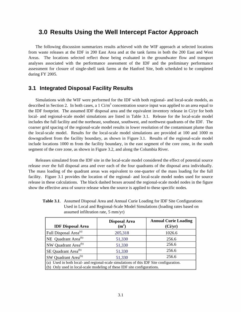
3.0 Results Using the Well Intercept Factor Approach ............................................................................. 3.1 3.1 Integrated Disposal Facility Results............................................................................................ 3.1 3.2 Tank Farm Area Results ............................................................................................................. 3.7

3.2.1 200 East Area Tank Farms ................................................................................................... 3.7 3.2.2 200 West Area Tank Farms................................................................................................ 3.11

4.0 Results Using the Convolution Approach ........................................................................................... 4.1

5.0 Comparison of Alternative Methods ................................................................................................... 5.1 5.1 Long-Term Increasing Release Scenario .................................................................................... 5.1 5.2 Shorter-Term Release Scenario................................................................................................... 5.4

6.0 Summary and Conclusions .................................................................................................................. 6.1

7.0 References ........................................................................................................................................... 7.1

xii

Figures 1.1 Schematic Representation of Computational Framework and Codes Used in the

Hanford Solid Waste Environmental Impact Statement .............................................................. 1.5 2.1 Comparison of Generalized Hydrogeologic and Geologic Stratigraphy ..................................... 2.2 2.2 Peripheral Boundaries Defined for the Three-Dimensional Model .............................................. 2.4 2.3 Transmissivity Distribution for the Unconfined Aquifer System Based on

Two-Dimensional Inverse Model Calibration .............................................................................. 2.6 2.4 Distribution of Estimated Hydraulic Conductivities at Water Table from Best-Fit

Inverse Calibration of Site-Wide Groundwater Model................................................................. 2.7 2.5 Distribution of Estimated Hydraulic Conductivities along Section Lines A-A’ and

B-B’ from Best-Fit Inverse Calibration of Site-Wide Groundwater Model .................................. 2.8 2.6 Predicted Post-Hanford Water Table Conditions........................................................................ 2.10 3.1 Grid Spaces Used to Simulate Contaminant Releases from the IDF in 200 East Area

and Associated 100- and 1000-m Lines of Analysis Used in Local-Scale Model ....................... 3.2 3.2 Location of IDF, Associated 1 km and Core Zone Lines of Analysis, and

Regional Model Grid Spacing ...................................................................................................... 3.2 3.3 Concentration Histories at 100 m for IDF Release Areas Using Local-Scale Model................... 3.3 3.4 Concentration Histories at 1000 m for IDF Release Areas Using Local-Scale Model................. 3.4 3.5 Comparison of Concentration Histories at Selected Points of Analysis for the Full

IDF Release Area and Recharge Rate of 5 mm/yr Using Regional-Scale Model......................... 3.6 3.6 Location of Nodes Used to Simulate Contaminant Releases for Aggregated Tank

Farms in 200 East Area in Regional-Scale Model Grid................................................................ 3.7 3.7 Location of Nodes Used to Simulate Contaminant Releases for Aggregated Tank

Farms in 200 West Area in Regional-Scale Model Grid .............................................................. 3.8 3.8 Concentration Histories at Segments of Core Zones for 200 East Tank Farm Release

Areas Using the Regional-Scale Model ........................................................................................ 3.9 3.9 Concentration Histories Along Columbia River for 200 East Tank Farm Release

Areas Using Regional-Scale Model.............................................................................................. 3.9 3.10 Concentration Histories at Segment Core Zones for 200 West Tank Farm Release

Areas Using the Regional-Scale Model ...................................................................................... 3.12 3.11 Concentration History Along Columbia River for 200 West Tank Farm Release

Areas Using the Regional-Scale Model ...................................................................................... 3.12 4.1 Concentration Histories at East Segment of Core Zone for Unit 10-year Release from IDF

and Aggregate Tank Farm in 200 East Area Using the Regional-Scale Model............................ 4.2 4.2 Concentration Histories Along the Columbia River for a Unit 10-year Release from IDF

and Aggregate Tank Farms in 200 East Area Using the Regional-Scale Model .......................... 4.2 4.3 Concentrations at the East Segment of the Core Zone for Unit 10-yr Release from the

Aggregate Tank Farms in 200 West Area Using Baseline Regional-Scale Model....................... 4.3 4.4 Concentrations Along the Columbia River for a Unit 10-yr Release from Aggregate

Tank Farms in 200 West Area Using the Regional-Scale Model ................................................. 4.3

xiii

5.1 Annual and Cumulative Long-Term Contaminant Release Example........................................... 5.2 5.2 Predicted 99Tc Concentrations at East Segment of Core Zone and Along the Columbia

River by Direct Simulation of Long-Term Source Release from ILAW Glass Wastes Containing 25,550 Ci of 99Tc near the IDF................................................................................... 5.2

5.3 Comparison of Predicted 99Tc Concentrations Using Direct Simulation with WIF and Convolution Approaches at Eastern Segment of Core Zone and Along Columbia River ............ 5.3

5.4 Annual and Cumulative Shorter-Term Contaminant Release Example ....................................... 5.5 5.5 Comparison of Predicted 99Tc Concentrations Using Direct Simulation with WIF and

Convolution Approaches at Eastern Segment of Core Zone and Along Columbia River ........ 5.5

Tables

2.1 Major Hydrogeologic Units Used in the Site-Wide Three-Dimensional Model .......................... 2.1 3.1 Assumed Disposal Area and Annual Curie Loading for IDF Site Configurations

Used in Local and Regional-Scale Model Simulations ................................................................ 3.1 3.2 WIFs at Selected Points of Analysis for Different IDF Release Areas and

Recharge Rates Using Local-Scale Model.................................................................................... 3.5 3.3 WIFs at Selected Points of Analysis for the Full IDF Release Area and

Recharge Rates Using Regional-Scale Model .............................................................................. 3.6 3.4 Assumed Tank Farm Areas and Annual Curie Loading Used in Regional-Scale

Model Simulations ........................................................................................................................ 3.8 3.5 WIFs at Selected Locations for 200 East Tank Farm Release Areas Using

Regional-Scale Model................................................................................................................. 3.10 3.6 Comparison of Ratios of Assumed Release Area to Largest Release Area in 200 East

and 200 West ............................................................................................................................. 3.11 3.7 WIFs at Selected Locations for 200 West Tank Farm Release Areas Using

Regional-Scale Model................................................................................................................. 3.13 4.1 Comparison of Unit Release Results at Core Zone and River for IDF and Tank Farm

Release Areas with Regional-Scale Model................................................................................... 4.1 5.1 Comparison of Predicted Peak 99Tc Concentrations Using Direct Simulation with WIF and

Convolution Approaches at East Segment of Core Zone and Along Columbia River ................. 5.4 5.2 Comparison of Predicted 99Tc Concentrations Using Direct Simulation with the WIF and

Convolution Approaches at East Segment of the Core Zone and Along Columbia River ........... 5.6

1.1

1.0 Introduction The purpose of this report is to summarize the results of numerical calculations that will support groundwater flow and transport analyses associated with the 2005 performance assessment of the Integrated Disposal Facility (IDF). This report also provides supporting information to other ongoing Hanford Site risk analyses associated with the closure of single-shell tank farms and related actions. The 2005 IDF performance assessment analysis will use well intercept factors (WIF) and methods that were outlined by Bergeron and Wurstner (2000) for the 2001 performance assessment of the IDF (Mann et al. 2001). The flow and transport analysis applied to the calculations summarized in this report employ both a Site-wide regional-scale model and a local-scale model of the area near the IDF. The regional-scale model was used to evaluate flow conditions, groundwater transport, and impacts from the IDF and individual tank farm areas near the core of the Hanford Site—around the 200 East and 200 West Areas and along the Columbia River. The local-scale model was used to evaluate impacts from the transport of contaminants at a hypothetical well 100 m downgradient from the IDF boundaries. Analyses similar to the regional-scale analysis of IDF releases are also provided at individual tank farm areas as additional information.

1.1 Background Several approaches are available to estimate the concentration of contaminants in groundwater from estimated mass releases to the aquifer. In this report we examine two of them. The first involves directly simulating the mass releases generated from process models of waste release and transport through the vadose zone to the underlying groundwater system at specific locations of interest. This approach requires that calculations be performed sequentially, with each simulation representing a unique inventory distribution and parameter set. It has been used extensively and is preferred when transient vadose zone and groundwater conditions are important and the number of combinations of inventory distributions and parameter sets is more than the number of simulations required. For assessments that consider only the impacts of future releases, after the effects of transient changes to the vadose zone and aquifer are considered less important, steady-state flow conditions can be assumed and alternative approaches used to estimate groundwater concentrations involving development of system output or response from a specified release at each source area. Background information on the WIF approach and another approach referred to in this report as the convolution approach is presented below. 1.1.1 Well Intercept Factor (WIF) Approach The WIF approach simulates the groundwater system response to a known concentration of a contaminant in water entering from the vadose zone over a specific water table surface area. This system response to a specific mass flux can be simulated independently. The ratio of estimated concentration in groundwater at a specific location to assumed contaminant concentration at the bottom of the vadose zone can be used to estimate groundwater concentrations at the same location from mass releases calculated independently with the waste release and vadose zone flow and transport process model. This approach can be useful for estimating groundwater concentrations at specific locations and can be a desirable

1.2

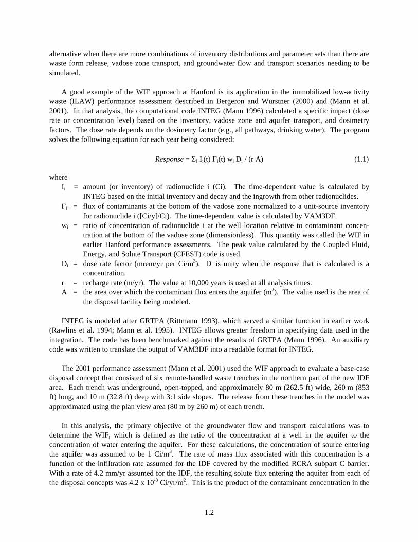
alternative when there are more combinations of inventory distributions and parameter sets than there are waste form release, vadose zone transport, and groundwater flow and transport scenarios needing to be simulated. A good example of the WIF approach at Hanford is its application in the immobilized low-activity waste (ILAW) performance assessment described in Bergeron and Wurstner (2000) and (Mann et al. 2001). In that analysis, the computational code INTEG (Mann 1996) calculated a specific impact (dose rate or concentration level) based on the inventory, vadose zone and aquifer transport, and dosimetry factors. The dose rate depends on the dosimetry factor (e.g., all pathways, drinking water). The program solves the following equation for each year being considered: Response = ΣI Ii(t) Γi(t) wi Di / (r A) (1.1) where

Ii = amount (or inventory) of radionuclide i (Ci). The time-dependent value is calculated by INTEG based on the initial inventory and decay and the ingrowth from other radionuclides.

Γi = flux of contaminants at the bottom of the vadose zone normalized to a unit-source inventory for radionuclide i ([Ci/y]/Ci). The time-dependent value is calculated by VAM3DF.

wi = ratio of concentration of radionuclide i at the well location relative to contaminant concen-tration at the bottom of the vadose zone (dimensionless). This quantity was called the WIF in earlier Hanford performance assessments. The peak value calculated by the Coupled Fluid, Energy, and Solute Transport (CFEST) code is used.

Di = dose rate factor (mrem/yr per Ci/m3). Di is unity when the response that is calculated is a concentration.

r = recharge rate (m/yr). The value at 10,000 years is used at all analysis times. A = the area over which the contaminant flux enters the aquifer (m2). The value used is the area of

the disposal facility being modeled.

INTEG is modeled after GRTPA (Rittmann 1993), which served a similar function in earlier work (Rawlins et al. 1994; Mann et al. 1995). INTEG allows greater freedom in specifying data used in the integration. The code has been benchmarked against the results of GRTPA (Mann 1996). An auxiliary code was written to translate the output of VAM3DF into a readable format for INTEG. The 2001 performance assessment (Mann et al. 2001) used the WIF approach to evaluate a base-case disposal concept that consisted of six remote-handled waste trenches in the northern part of the new IDF area. Each trench was underground, open-topped, and approximately 80 m (262.5 ft) wide, 260 m (853 ft) long, and 10 m (32.8 ft) deep with 3:1 side slopes. The release from these trenches in the model was approximated using the plan view area (80 m by 260 m) of each trench. In this analysis, the primary objective of the groundwater flow and transport calculations was to determine the WIF, which is defined as the ratio of the concentration at a well in the aquifer to the concentration of water entering the aquifer. For these calculations, the concentration of source entering the aquifer was assumed to be 1 Ci/m3. The rate of mass flux associated with this concentration is a function of the infiltration rate assumed for the IDF covered by the modified RCRA subpart C barrier. With a rate of 4.2 mm/yr assumed for the IDF, the resulting solute flux entering the aquifer from each of the disposal concepts was 4.2 x 10-3 Ci/yr/m2. This is the product of the contaminant concentration in the

1.3

infiltrating water and the infiltration rate. In all simulations performed, the WIF was calculated at a hypothetical well approximately 100 m (328 ft) downgradient from the boundary of the IDF site along the centerline of the simulated plume.

Transport model results for the remote-handled trench concept were based on local-scale flow conditions. These conditions were developed based on boundary conditions provided by the steady-state simulation of future post-Hanford flow conditions performed with the Hanford Site-wide model (Cole et al 2001a, b). Under the post-Hanford flow conditions represented in this analysis, groundwater moves across the IDF site in a southeasterly direction before exiting the local-scale model in the southeast corner of 200 East Area. 1.1.2 Convolution Approach The convolution approach for estimating groundwater concentrations, conceptually described in Lee (1999), simulates a system response from a unit inventory release through each of three process models (i.e., source release, vadose zone flow and transport, and groundwater flow and transport). It then uses the results with principles of superposition to estimate groundwater concentrations for a specific constituent inventory distribution. A unit release in each process model can be simulated independently. Then, by making the assumption of linearity, the unit release responses from each individual source area with each of the process models can be combined or superimposed. This approach can be useful in estimating groundwater concentrations at specific locations and can be a preferred alternative when there are more combinations of inventory distributions and parameter sets than there are vadose zone and groundwater flow and transport scenarios needing to be simulated. In the convolution approach, the concentration in the groundwater at a specific location i at time t (Ci,t) can be estimated using Equations 1.2 and 1.3:

)(f1 1

1,,,, ∑ ∑= =Τ

+Τ−ΤΜ=n

s

t

tisssti cC (1.2)

1,1

,, (f +Τ−=Τ

Τ∑= ts

t

sts fr ) (1.3)

where tiC , = concentration at location i at time t

sM = inventory at source s

tisc ,, = groundwater concentration at i based on a unit release from s (CFEST model output)

tsr , = fractional release of unit inventory in source s at time t (release model output)

tsf , = flux to water table from source s at time t based on unit release from s

(Subsurface Transport over Multiple Phases [STOMP] model output) n = number of sources Τ = time integration variable.

1.4

and tisc ,, and tsf , are the discrete response functions estimated with the vadose zone and groundwater

models based on a unit release. These discrete responses can be combined easily with Equations 1.2 and 1.3 (that is, superimposed) in a variety of ways to estimate system response to different inventory distributions and parameter sets. (Equations 1.2 and 1.3 are discrete approximations of the classic convolution approach used in calculating superposition of responses in linear response systems.) The form of Equation 1.2 was also used to estimate the time-varying flux of a contaminant to the Columbia River by substituting the groundwater concentration based on a unit release from s with the calculated flux to the river based on a unit release from s. This river flux was combined with average annual flow in the Columbia River to estimate concentration levels that are the basis for potential human health impacts and ecosystem risk from exposure to Columbia River water. A good example of the convolution approach at Hanford was its application to analyze the potential impacts from the subsurface transport pathway for the low-level waste burial grounds (LLBGs), as described in the Hanford Solid Waste Environmental Impact Statement (DOE/RL 2004). In this analysis, contaminant inventory for the LLBGs was assumed to be released to the vadose zone according to an appropriate model. Transport within the vadose zone was estimated with a steady-state, one-dimensional, variably saturated vadose zone transport model by assuming a unit release for a range of recharge rates. Travel times for releases of unit mass were defined by arrival of 50 percent of each unit mass. These travel times were used to translate mass releases from the LLBGs into mass releases at the water table. The time-varying mass flux arriving at the water table reflects the entire time history of the mass release from the source area as well as the calculated travel time in the vadose zone. Estimates of contaminant release transport from the LLBGs to the groundwater were evaluated by first calculating transport of 10-year releases of a unit of dry mass into the unconfined aquifer at the LLBGs at the water table. These transport calculations were made with a steady-state, three-dimensional, saturated groundwater flow and transient transport model. These calculated concentrations, based on a unit release, were then used in the convolution approach to translate transport of mass releases from the LLBG through the vadose zone and the aquifer to specified locations downgradient from the source areas. The concentrations in the groundwater plumes for each radionuclide were translated into doses using methods described in Appendix F of DOE/RL (2004). The sequence of calculations in the long-term assessment required estimation of the potential ground-water quality impacts using a suite of process models that estimate source-term release, vadose zone flow and transport, and groundwater flow and transport. The computational framework for these process models and the relationship of software elements, schematically illustrated in Figure 1.1, is as follows:

1. Excel™ workbook

2. Dynamically linked library version of the STOMP code (White and Oostrom 1996, 1997; Nichols et al. 1997)

3. CFEST code (Gupta 1987, 1997).

1.5

Figure 1.1. Schematic Representation of Computational Framework and Codes Used in the Hanford Solid Waste Environmental Impact Statement (DOE/RL 2004)

The convolution approach and the implicit assumption of linearity are reasonable for approximating the long-term release of constituents from solid waste disposal facilities for the following reasons:

The environment of solid waste sources in Hanford solid waste disposal facilities has been characterized as low-organic, low-salt, and nearly neutral geochemically (Kincaid et al. 1998), and processes such as nonlinear adsorption and other complex chemical reactions are not expected to have a substantial effect on contaminant release and transport through the vadose zone and groundwater at the scales of interest (that is, 100 m downgradient from the waste facilities toward the Columbia River).

Wastes disposed in Hanford solid waste disposal facilities are largely dry solids with no substantial amounts of liquids or complex chemical fluids that could enhance migration of constituents to the underlying water table.

Waste releases are expected to occur over long periods and will likely reach the water table when the effect of past artificial discharges has dissipated and the unconfined aquifer returns to more natural conditions. Using estimates of infiltration through the vadose zone to the underlying groundwater that would reflect long-term average rates of natural recharge appears reasonable.

1.2 Purpose and Scope of Report The primary purpose of this report is to summarize calculations using the WIF approach that support groundwater flow and transport analyses associated with the 2005 performance assessment of the IDF. This document can be referenced for WIF calculations for the IDF PA and can provide supporting information to other ongoing Hanford Site risk analyses associated with the closure of single-shell tank farms and related actions.

1.6

Because the Site-wide model that supports these calculations is being recalibrated to incorporate current data, this report is being made available electronically to a limited number of onsite personnel. Many of the calculations in this report will be redone using the recalibrated model when it becomes available later this year. The report will be reissued when the updated calculations are completed, to support ongoing maintenance of the IDF PA. Meanwhile, an electronic version of this report can be accessed online using the search feature at http://www.pnl.gov/main/publications/. Section 2 describes the conceptual and numerical groundwater flow and transport model that provided the basis for the simulated results summarized in this report. Section 3 summarizes results using the WIF approach at selected waste release locations from the IDF in the 200 East Area and from tank farms in the 200 East and 200 West Areas. Section 4 summarizes results using the convolution approach for the same sites and waste releases. To see how the WIF approach compares with the convolution approach for estimating groundwater concentrations from mass releases to the unconfined aquifer, groundwater concentrations were estimated with the both approaches for two hypothetical release scenarios. Results for the two release scenarios are summarized and compared in Section 5. Section 6 discusses our conclusions, and Section 7 contains cited references.

2.1

2.0 Conceptual and Numerical Groundwater Model Used in Analyses

This section describes the conceptual and numerical groundwater flow and transport models used to develop results for the approaches summarized in this report. For these analyses, contaminant transport was simulated with the three-dimensional Site-wide groundwater flow and transport model of the unconfined aquifer described in Cole et al. (2001a)

2.1 Hydrogeologic Framework The major hydrogeologic units that make up the unconfined aquifer system simulated in the Hanford Site-wide model are described briefly in Table 2.1. A graphic comparison of the model units taken from Thorne et al. (1993) with the major units of the stratigraphic column defined in Lindsey (1995) is shown in Figure 2.1. Although nine hydrogeologic units were defined in this framework, only seven (Units 1, 4, 5, 6, 7, 8, and 9) were generally found to be below the water table during post-Hanford conditions (Cole et al. 1997, 2001). These are the odd-numbered Ringold model units (5, 7, and 9), which are predominantly coarse-grained sediments; the even-numbered Ringold model units (4, 6, and 8), which are predominantly fine-grained sediments with low permeability; and the Hanford formation and pre-Missoula gravel deposits combined, which were designated as Model Unit 1. Model Units 2 and 3, comprising the early Palouse soil and Plio-Pleistocene deposits, respectively, lie above the current water table. The predominantly mud facies of the upper Ringold unit identified by Lindsey (1995) was designated Model Unit 4. However, the lower, predominantly sand portion of the upper Ringold unit described in Lindsey (1995) was grouped with Model Unit 5, which also includes Ringold gravel/sand Units E and C, because the predominantly sand portion of the upper Ringold is expected to have hydraulic properties similar to Units E and C. The lower mud unit identified by Lindsey (1995) was designated as Model Units 6 and 8. Where they exist, the

Table 2.1. Major Hydrogeologic Units Used in the Site-Wide Three-Dimensional Model

Unit Number Hydrogeologic Unit Lithologic Description

1 Hanford Formation Fluvial gravels and coarse sands 2 Palouse Soils Fine-grained sediments and eolian silts 3 Plio-Pleistocene Unit Buried soil horizon containing caliche and

basaltic gravels 4 Upper Ringold Formation Fine-grained fluvial/lacustrine sediments 5 Middle Ringold (Units E and C) Semi-indurated coarse-grained fluvial

sediments 6 Middle Ringold (Lower Ringold Mud) Fine-grained sediments with some inter-

bedded coarse-grained sediments 7 Middle Ringold (Units B and D) Coarse-grained sediments 8 Lower Mud Sequence (Lower Ringold

and part of Basal Ringold mud units) Lower blue or green clay or mud sequence

9 Basal Ringold (Unit A) Fluvial sand and gravel 10 Columbia River Basalt Basalt

2.2

Figure 2.1. Comparison of Generalized Hydrogeologic and Geologic Stratigraphy [from Thorne et al. (1993) and after Lindsey (1995)]

gravel and sand Units B and D within the lower Ringold were designated Model Unit 7. Gravels of Ringold Unit A were designated as Model Unit 9, and the underlying basalt was designated as Model Unit 10. The basalt was assigned a very low hydraulic conductivity and was treated as essentially impermeable in the model. The lateral extent and thickness of each hydrogeologic unit were defined based on information from drillers’ well logs, geologists’ logs, geophysical logs, and an understanding of the geologic environment.

2.3

These interpreted areal distributions and thicknesses were then integrated into EarthVision™ (Dynamic Graphics, Inc., Alameda, CA), a three-dimensional visualization software package that was used to construct a database of the three-dimensional hydrogeologic framework. 2.1.1 Recharge and Flow System Boundary Conditions The Site-wide groundwater model (Cole et al. 2001a) considered both natural and artificial recharge to the aquifer. Natural recharge to the unconfined aquifer system occurs from infiltration of 1) runoff from elevated regions along the western boundary of the Hanford Site, 2) spring discharges originating from the basalt-confined aquifer system and along the western boundary, and 3) precipitation falling across the Site. Some recharge also occurs along the Yakima River in the southern portion of the Site. Natural recharge from runoff and irrigation in the Cold Creek and Dry Creek Valleys, upgradient from the Site, also provide a source of groundwater inflow. Natural recharge from precipitation on the Site is highly variable, both spatially and temporally, and depends on local climate, soil type, and vegetation. The other source of recharge to the unconfined aquifer has historically come from wastewater disposal. The large volume of artificial recharge from wastewater discharged from disposal facilities on the Hanford Site over the past 60 years has substantially affected groundwater flow and contaminant transport in the unconfined aquifer system. This volume of artificial recharge has decreased significantly in the past 10 years, and the water table has declined steadily. After Site closure, the unconfined aquifer system eventually will reach more natural conditions. Because flow conditions simulated for this assessment focus on conditions that are likely to exist after closure and well into the future, the effects of past and current wastewater discharges on the unconfined aquifer system were not considered. Peripheral boundaries defined for the three-dimensional model are shown in Figure 2.2 along with the three-dimensional flow-model grid. The flow system is bounded by the Columbia River on the north and east and by the Yakima River and basalt ridges on the south and west. The Columbia River represents a point of regional discharge for the unconfined aquifer system. The amount of groundwater discharged to the river is a function of local hydraulic gradient between the groundwater elevation adjacent to the river and the river-stage elevation. This hydraulic gradient is highly variable because the river stage is affected by releases from upstream dams. Because of the regional scale and long timeframe considered in this assessment, Site-wide flow and transport modeling did not include the short-term and local-scale transient effects of the Columbia River system on the unconfined aquifer. However, the long-term effect of the Columbia River as a regional discharge area for the unconfined aquifer system was approximated in the three-dimensional model with a held-head boundary applied at the uppermost nodes of the model at the river’s approximate left bank and channel midpoint. Nodes representing the thickness of the aquifer below those representing the midpoint of the river channel were treated as no-flow boundaries. This boundary condition was used to approximate the groundwater divide that exists beneath the river where groundwater from the Hanford Site and the other side of the river discharge into the Columbia. This head boundary was held constant at the long-term, average river stage elevations implemented in the Site-wide model based on results from previous work (Walters et al. 1994) for the Columbia River with the CHARIMA model. The Yakima River was also represented as a constant head boundary at surface nodes approximating its location and average flow and stage. Like the Columbia, nodes representing the thickness of the aquifer below the Yakima’s channel were treated as no-flow boundaries. Short-term fluctuations in level do not influence modeling results.

2.4

Figure 2.2. Peripheral Boundaries Defined for the Three-Dimensional Model (after Cole et al. 1997)

In the Cold Creek and Dry Creek Valleys, the unconfined aquifer system extends westward beyond the boundary of the model. To approximate the groundwater flux entering the modeled area from these valleys, both constant-head and constant-flux boundary conditions were defined. A constant-head boundary condition was specified for Cold Creek Valley for the steady-state model calibration runs. The fluxes resulting from the specified-head boundaries in the calibrated steady-state model were then used in the steady-state simulation of flow conditions after Hanford Site closure. The constant-flux boundary was

2.5

used because it represents the response of the boundary to a declining water table better than a constant-head boundary does. Discharges from Dry Creek Valley resulting from infiltration of precipitation and spring discharges are approximated using the same methods. The basalt underlying the unconfined aquifer sediments represents a lower boundary for the system. The potential for interflow (recharge and discharge) between the basalt-confined and unconfined aquifer systems is largely unquantified, but it is postulated to be small relative to the other flow components estimated for the unconfined aquifer system (Cole et al. 1997, 2001a, b). Therefore, interflow with underlying basalt units was not included in the three-dimensional model. The basalt was defined in the model as an essentially impermeable unit underlying the sediments. 2.1.2 Flow and Transport Properties The development of estimates of flow and transport properties in the Hanford Site-wide model is described in detail in Wurstner (1995) and Cole et al. (1997, 2001a). In the original calibration procedure described in Wurstner et al. (1995), measured transmissivity values of the aquifer were used in a two-dimensional model with an inverse calibration procedure to determine the transmissivity distribution of the unconfined aquifer system. Hydraulic head conditions for 1979 were used in the inverse calibration because measured hydraulic heads were relatively stable at that time. Details about the updated calibration of the two-dimensional model are provided in Cole et al. (1997). The resulting transmissivity distribution for the unconfined aquifer system is shown in Figure 2.3. Hydraulic conductivities were assigned to the three-dimensional model units so the total aquifer transmissivity from inverse calibration was preserved at every location. The vertical distribution of hydraulic conductivity at each spatial location was determined based on the transmissivity value and other information, including facies descriptions and hydraulic property values measured for similar facies. A complete description of the seven-step process used to distribute the transmissivity vertically among the model’s hydrogeologic units is presented in Cole et al. (1997). The current version of the Site-wide model relies on a three-dimensional representation of the aquifer system that was calibrated to groundwater monitoring data collected during Hanford operations from 1943 to the present. The calibration procedure and results for this model are described in Cole et al. (2001a). This recent work is part of a broader effort to develop and implement a stochastic uncertainty estimation methodology in future assessments and analyses using the Site-wide groundwater model (Cole et al. 2001b). The resulting distribution of hydraulic conductivities from this recent calibration effort is provided in Figures 2.4 and 2.5. Information on transport properties used in this analysis relied on parameters developed in past modeling studies at the Hanford Site (Wurstner et al. 1995). Estimates of selected model parameters were developed to account for contaminant transport dispersion in all simulations. Specific model parameters required included longitudinal and transverse dispersivity (DL and DT) and effective porosity.

2.6

Figure 2.3. Transmissivity Distribution for the Unconfined Aquifer System Based on Two- Dimensional Inverse Model Calibration (after Wurstner et al. 1995)

2.7

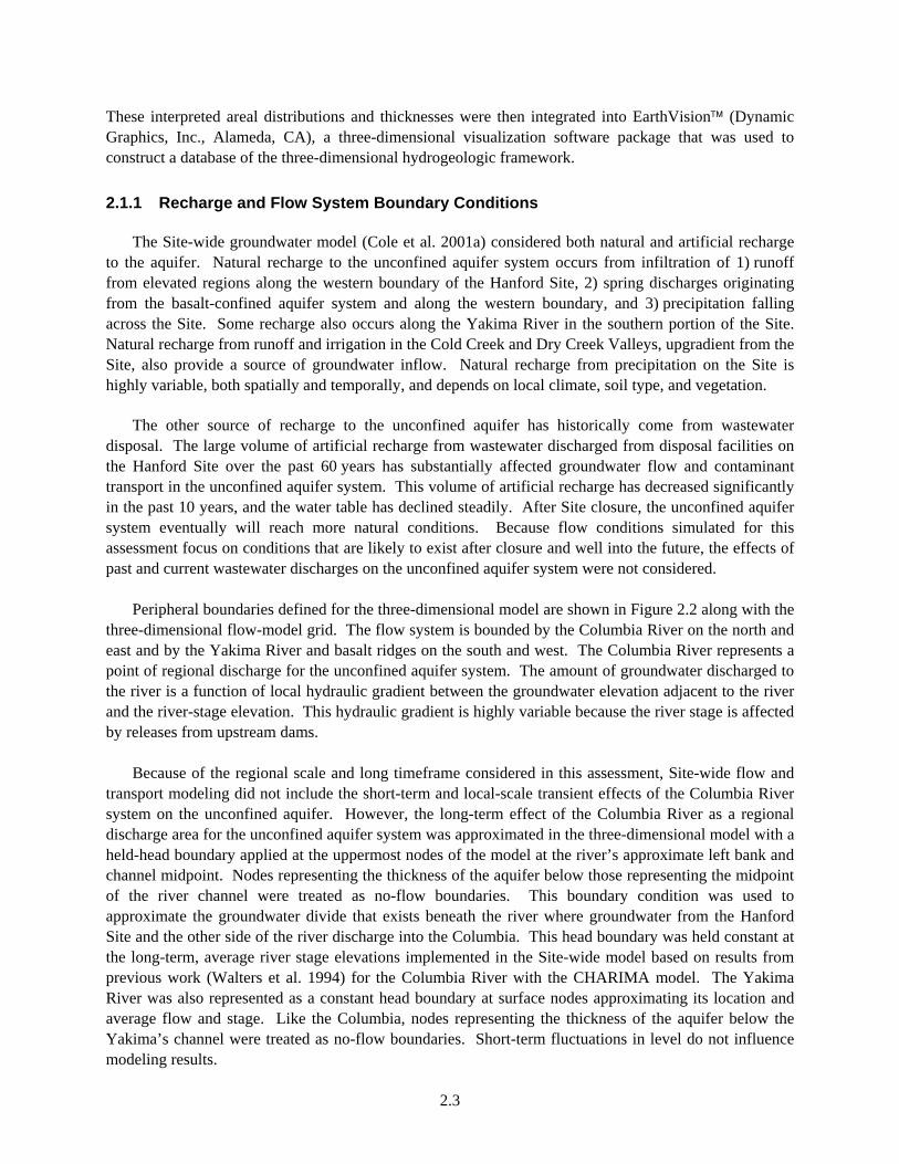
Figure 2.4. Distribution of Estimated Hydraulic Conductivities at Water Table from Best-Fit Inverse Calibration of Site-Wide Groundwater Model (after Cole et al. 2001a)

For this analysis, a longitudinal dispersivity, DL, of 95 m (310 ft) was selected based on the scale of interest. Although transport results produced in this analysis span a range of scales, the key scale of interest is the minimum distance between some of the source areas in the Central Plateau and the buffer zone boundary surrounding this area. For some sources in 200 East Area, the distance of interest is on the order of 1 to 2 km. Thus, a dispersivity value used in the original analysis was selected to be approximately equal to 10 percent of the minimum travel distance of interest of about 1 km (0.6 mi).

2.8

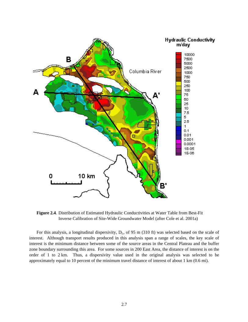
Figure 2.5. Distribution of Estimated Hydraulic Conductivities along Section Lines A-A’ and B-B’ from Best-Fit Inverse Calibration of Site-Wide Groundwater Model (after Cole et al. 2001a)

The longitudinal dispersivity was also selected to be consistent with the range of recommended grid Peclet numbers (Pe <4) to reach an acceptable solution. The 95-m (310-ft) estimate is about one-fourth of the grid spacing in the finest part of the model grid in the Central Plateau, where the smallest grid spacing is about 375 x 375 m (1230 × 1230 ft). The corresponding transverse dispersivity used in the analysis was selected to be consistent with general available regulatory and technical guidance. EPA guidance on the subject suggests a 1 to 3 ratio for DT to DL (Mills et al. 1985). Freeze and Cherry (1979) report that transverse dispersivities are normally lower than longitudinal dispersivities by a factor of 5 to 20 (that is, 0.2 to 0.05). Walton (1985) states that reported ratios of DT to DL vary from 1 to 24, but common values are 0.2 and 0.1. Considering this information, a transverse dispersivity, DT, used in Composite Analysis simulations (Kincaid et al. 1998) was assumed to be about 20 m (65.6 ft), which is approximately 20 percent of the selected longitudinal dispersivity. The effective porosity was estimated from specific yields obtained from multiple-well aquifer tests. These values range from 0.01 to 0.37. Laboratory measurements of porosity that range from 0.19 to 0.41

2.9

were available for samples from a few Hanford wells and were also considered. The few tracer tests conducted indicate effective porosities ranging from 0.1 to 0.25. Within the model, a porosity value of 0.21 was used for the Ringold Formation (Model Unit 5), and a value of 0.07 was used for the Hanford Formation (Model Unit 1) to be consistent with specific yield estimates for these units obtained from inverse model calibration by Cole et al. (2001). Porosity values of other Ringold Model Units (Units 4, 6, 7, 8, and 9) were set at a value of 0.1. For the lower water table conditions expected during the post-Hanford period, the Early Palouse and Plio-Pleistocene hydrogeologic units (Model Units 2 and 3) existed above the projected water table and so were not considered in the analysis. To support calculations made at the IDF boundary in this analysis, additional calculations 100-m downgradient from the IDF boundary were developed using a more refined local-scale version of the regional-scale model. The distributions of hydraulic characteristics and geometry of major hydrogeologic units used in the local-scale model were based on the interpolation of regional-scale model characteristics and interpretation of major units onto the local-scale model grids. Like the regional-scale transport simulations, calculations were performed for post-Hanford conditions, as described in Section 2.2. In the local-scale analysis, a longitudinal dispersivity, DL, of 10 m (33 ft) was selected to be approx-imately equal to 10 percent of the minimum travel distance of interest of about 100 m. A transverse dispersivity of about 20 percent of the longitudinal dispersivity, or 2 m, was also used in the analysis.

2.2 Simulation of Post-Closure Flow Conditions Past projections of water table conditions after Site closure have estimated the impact of Hanford operations ending, and the resulting changes in artificial discharges have been used extensively as a part of Site waste management practices (Hartman 2000). Simulations of transient-flow conditions from 1944 through the year 3050 were conducted by Bryce et al. (2002). Their three-dimensional model shows an overall decline in the hydraulic head and hydraulic gradient across the entire water table within the modeled region. These simulations suggest that the groundwater flow in portions of the unconfined aquifer would reach steady state in 100 to 350 years. The results were generally consistent with findings for similar conditions in earlier modeling by Cole et al. (1997) and Kincaid et al. (1998). Given the expected long delay for contaminants from potential long-term releases from the IDF and tank farm areas to reach the groundwater, the hydrologic framework of all groundwater transport calculations was based on a postulated post-Hanford, steady-state water table estimated with the three-dimensional model. These conditions would only reflect estimated boundary condition fluxes (for example, natural recharge and lateral boundary fluxes), not the effect of past and current wastewater discharges, on the unconfined aquifer system. Flow modeling results also suggest that, as water levels drop in the central areas where the basalt crops out above the water table, the saturated thickness of the unconfined aquifer will decrease, and portions of the aquifer may actually dry out. This thinning/drying of the aquifer is predicted to occur in the area just north of the 200 East Area between Gable Butte and the outcrop south of Gable Mountain. The drying would separate this northern area of the unconfined aquifer hydrologically from the area south of Gable Mountain and Gable Butte. Because of the uncertainty in the potential natural recharge and boundary fluxes from upgradient areas, the potential movement of contaminants through the gap or east toward the Columbia River is also uncertain.

2.10

For this analysis, flow conditions reflective of assumed basalt subcrops north of the 200 East Area that effectively cut off the flow and transport from both the 200 East and West Areas to the north through the gap between Gable Mountain and Gable Butte were considered (see Figure 2.6). The extent of subcrops of basalt bedrock shown in this figure was developed by comparing predictions of the water table with the current interpretation and potential uncertainty of the top of underlying basalt. This assumed basalt subcrop distribution and the associated flow condition lead to a predominant easterly flow from most of the 200 East and West Areas. This easterly flow scenario is consistent with that used in supporting groundwater flow and transport calculations from the original ILAW performance assessment (Bergeron and Wurstner 2000; Mann et al. 2001) and the preliminary IDF risk assessment (Mann et al. 2003a, b). This flow condition is also considered for some of the transport simulations evaluated in the Solid Waste Environmental Impact Statement (DOE/RL 2004).

Figure 2.6. Predicted Post-Hanford Water Table Conditions (predominant easterly flow)

3.1

3.0 Results Using the Well Intercept Factor Approach The following discussion summarizes results achieved with the WIF approach at selected locations from waste releases at the IDF in 200 East Area and at the tank farms in both the 200 East and West Areas. The locations selected reflect those being evaluated in the groundwater flow and transport analyses associated with the performance assessment of the IDF and the preliminary performance assessment for closure of single-shell tank farms at the Hanford Site, both scheduled to be completed during FY 2005.

3.1 Integrated Disposal Facility Results Simulations with the WIF were performed for the IDF with both regional- and local-scale models, as described in Section 2. In both cases, a 1 Ci/m3 concentration source input was applied to an area equal to the IDF footprint. The assumed IDF disposal area and the equivalent inventory release in Ci/yr for both local- and regional-scale model simulations are listed in Table 3.1. Release for the local-scale model includes the full facility and the northeast, southeast, southwest, and northwest quadrants of the IDF. The coarser grid spacing of the regional-scale model results in lower resolution of the contaminant plume than the local-scale model. Results for the local-scale model simulations are provided at 100 and 1000 m downgradient from the facility boundary, as shown in Figure 3.1. Results of the regional-scale model include locations 1000 m from the facility boundary, in the east segment of the core zone, in the south segment of the core zone, as shown in Figure 3.2, and along the Columbia River. Releases simulated from the IDF site in the local-scale model considered the effect of potential source release over the full disposal area and over each of the four quadrants of the disposal area individually. The mass loading of the quadrant areas was equivalent to one-quarter of the mass loading for the full facility. Figure 3.1 provides the location of the regional- and local-scale model nodes used for source release in these calculations. The black dashed boxes around the regional-scale model nodes in the figure show the effective area of source release when the source is applied to these specific nodes.

Table 3.1. Assumed Disposal Area and Annual Curie Loading for IDF Site Configurations Used in Local and Regional-Scale Model Simulations (loading rates based on assumed infiltration rate, 5 mm/yr)

IDF Disposal Area Disposal Area

(m2) Annual Curie Loading

(Ci/yr) Full Disposal Area(a) 205,318 1026.6 NE Quadrant Area(b) 51,330 256.6 NW Quadrant Area(b) 51,330 256.6 SE Quadrant Area(b) 51,330 256.6 SW Quadrant Area(b) 51,330 256.6 (a) Used in both local- and regional-scale simulations of this IDF Site configuration. (b) Only used in local-scale modeling of these IDF site configurations.

3.2

IDF Boundary

1 km Compliance Boundary100 m Compliance Boundary

Regional IDF nodes

Easting (m)

Nor

thin

g(m

)

574000 574500 575000 575500 576000 576500

134000

134500

135000

135500

136000

YEAR 1.0 Figure 3.1. Grid Spaces Used to Simulate Contaminant Releases from the IDF in 200 East Area and Associated 100- and 1000-m Lines of Analysis Used in Local-Scale Model (nodes used to approximate contaminant release from IDF in regional-scale model shown as red dots)

Easting (m)

Nor

thin

g(m

)

565000 570000 575000

130000

132000

134000

136000

138000

140000

142000

144000

YEAR 0

Core Zone Boundary

IDF FacilityBoundary

1 km Point ofAnalysis

Figure 3.2. Location of IDF, Associated 1 km and Core Zone Lines of Analysis, and Regional Model Grid Spacing

3.3

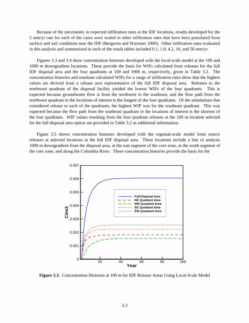
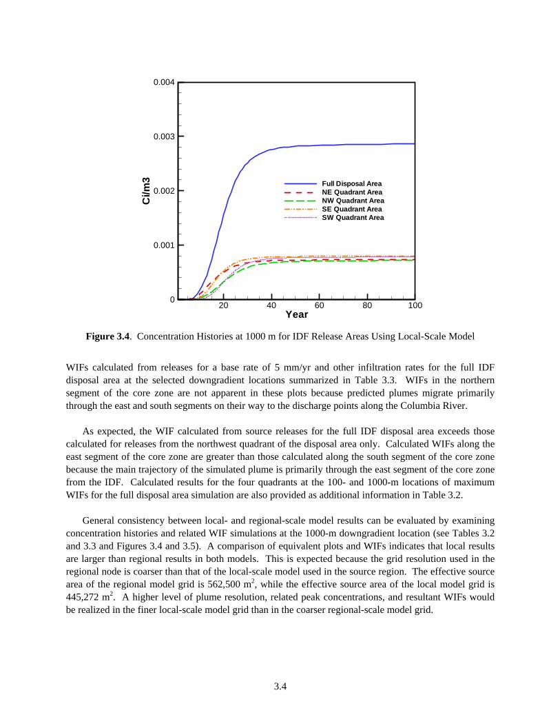
Because of the uncertainty in expected infiltration rates at the IDF locations, results developed for the 5 mm/yr rate for each of the cases were scaled to other infiltration rates that have been postulated from surface and soil conditions near the IDF (Bergeron and Wurstner 2000). Other infiltration rates evaluated in this analysis and summarized in each of the result tables included 0.1, 1.0, 4.2, 10, and 50 mm/yr. Figures 3.3 and 3.4 show concentration histories developed with the local-scale model at the 100 and 1000 m downgradient locations. These provide the basis for WIFs calculated from releases for the full IDF disposal area and the four quadrants at 100 and 1000 m, respectively, given in Table 3.2. The concentration histories and resultant calculated WIFs for a range of infiltration rates show that the highest values are derived from a release area representative of the full IDF disposal area. Releases to the northwest quadrant of the disposal facility yielded the lowest WIFs of the four quadrants. This is expected because groundwater flow is from the northwest to the southeast, and the flow path from the northwest quadrant to the locations of interest is the longest of the four quadrants. Of the simulations that considered release to each of the quadrants, the highest WIF was for the southeast quadrant. This was expected because the flow path from the southeast quadrant to the locations of interest is the shortest of the four quadrants. WIF values resulting from the four quadrant releases at the 100 m location selected for the full disposal area option are provided in Table 3.2 as additional information. Figure 3.5 shows concentration histories developed with the regional-scale model from source releases at selected locations in the full IDF disposal area. These locations include a line of analysis 1000 m downgradient from the disposal area, at the east segment of the core zone, at the south segment of the core zone, and along the Columbia River. These concentration histories provide the basis for the

Year

Ci/m

3

20 40 60 80 1000

0.001

0.002

0.003

0.004

0.005

0.006

0.007

Full Disposal AreaNE Quadrant AreaNW Quadrant AreaSE Quadrant AreaSW Quadrant Area

Figure 3.3. Concentration Histories at 100 m for IDF Release Areas Using Local-Scale Model

3.4

Year

Ci/m

3

20 40 60 80 1000

0.001

0.002

0.003

0.004

Full Disposal AreaNE Quadrant AreaNW Quadrant AreaSE Quadrant AreaSW Quadrant Area

Figure 3.4. Concentration Histories at 1000 m for IDF Release Areas Using Local-Scale Model

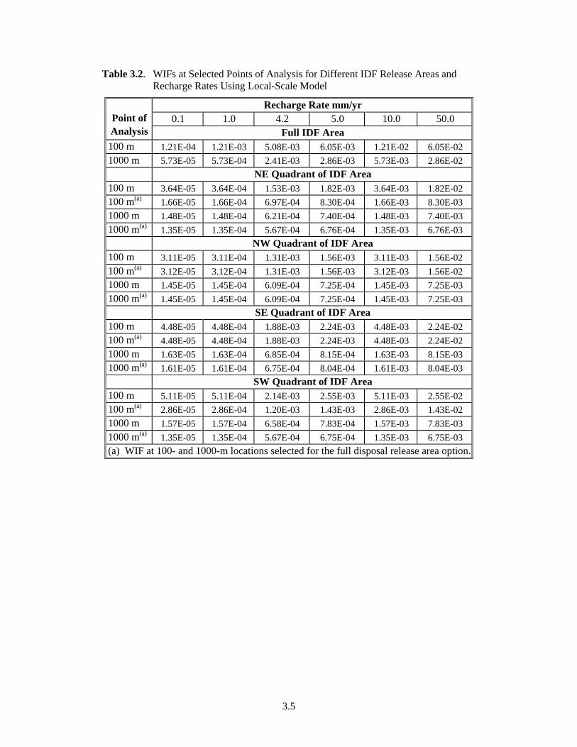
WIFs calculated from releases for a base rate of 5 mm/yr and other infiltration rates for the full IDF disposal area at the selected downgradient locations summarized in Table 3.3. WIFs in the northern segment of the core zone are not apparent in these plots because predicted plumes migrate primarily through the east and south segments on their way to the discharge points along the Columbia River. As expected, the WIF calculated from source releases for the full IDF disposal area exceeds those calculated for releases from the northwest quadrant of the disposal area only. Calculated WIFs along the east segment of the core zone are greater than those calculated along the south segment of the core zone because the main trajectory of the simulated plume is primarily through the east segment of the core zone from the IDF. Calculated results for the four quadrants at the 100- and 1000-m locations of maximum WIFs for the full disposal area simulation are also provided as additional information in Table 3.2. General consistency between local- and regional-scale model results can be evaluated by examining concentration histories and related WIF simulations at the 1000-m downgradient location (see Tables 3.2 and 3.3 and Figures 3.4 and 3.5). A comparison of equivalent plots and WIFs indicates that local results are larger than regional results in both models. This is expected because the grid resolution used in the regional node is coarser than that of the local-scale model used in the source region. The effective source area of the regional model grid is 562,500 m2, while the effective source area of the local model grid is 445,272 m2. A higher level of plume resolution, related peak concentrations, and resultant WIFs would be realized in the finer local-scale model grid than in the coarser regional-scale model grid.

3.5

Table 3.2. WIFs at Selected Points of Analysis for Different IDF Release Areas and Recharge Rates Using Local-Scale Model

Recharge Rate mm/yr 0.1 1.0 4.2 5.0 10.0 50.0 Point of

Analysis Full IDF Area 100 m 1.21E-04 1.21E-03 5.08E-03 6.05E-03 1.21E-02 6.05E-02 1000 m 5.73E-05 5.73E-04 2.41E-03 2.86E-03 5.73E-03 2.86E-02 NE Quadrant of IDF Area 100 m 3.64E-05 3.64E-04 1.53E-03 1.82E-03 3.64E-03 1.82E-02 100 m(a) 1.66E-05 1.66E-04 6.97E-04 8.30E-04 1.66E-03 8.30E-03 1000 m 1.48E-05 1.48E-04 6.21E-04 7.40E-04 1.48E-03 7.40E-03 1000 m(a) 1.35E-05 1.35E-04 5.67E-04 6.76E-04 1.35E-03 6.76E-03 NW Quadrant of IDF Area 100 m 3.11E-05 3.11E-04 1.31E-03 1.56E-03 3.11E-03 1.56E-02 100 m(a) 3.12E-05 3.12E-04 1.31E-03 1.56E-03 3.12E-03 1.56E-02 1000 m 1.45E-05 1.45E-04 6.09E-04 7.25E-04 1.45E-03 7.25E-03 1000 m(a) 1.45E-05 1.45E-04 6.09E-04 7.25E-04 1.45E-03 7.25E-03 SE Quadrant of IDF Area 100 m 4.48E-05 4.48E-04 1.88E-03 2.24E-03 4.48E-03 2.24E-02 100 m(a) 4.48E-05 4.48E-04 1.88E-03 2.24E-03 4.48E-03 2.24E-02 1000 m 1.63E-05 1.63E-04 6.85E-04 8.15E-04 1.63E-03 8.15E-03 1000 m(a) 1.61E-05 1.61E-04 6.75E-04 8.04E-04 1.61E-03 8.04E-03 SW Quadrant of IDF Area 100 m 5.11E-05 5.11E-04 2.14E-03 2.55E-03 5.11E-03 2.55E-02 100 m(a) 2.86E-05 2.86E-04 1.20E-03 1.43E-03 2.86E-03 1.43E-02 1000 m 1.57E-05 1.57E-04 6.58E-04 7.83E-04 1.57E-03 7.83E-03 1000 m(a) 1.35E-05 1.35E-04 5.67E-04 6.75E-04 1.35E-03 6.75E-03 (a) WIF at 100- and 1000-m locations selected for the full disposal release area option.

3.6

Year

Ci/m

3

200 400 600 800 10000

0.0002

0.0004

0.0006

0.0008

0.001

0.0012

Full Disposal Area - 1000mFull Disposal Area - East Core ZoneFull Disposal Area - RiverFull Disposal Area - South Core Zone

Figure 3.5. Comparison of Concentration Histories at Selected Points of Analysis for the Full IDF Release Area and Recharge Rate of 5 mm/yr Using Regional-Scale Model (results for north, east, and south core locations represent maximum concentrations estimated along the respective segments of the core zone downgradient from the source areas)

Table 3.3. WIFs at Selected Points of Analysis for the Full IDF Release Area and Recharge Rates Using Regional-Scale Model

Recharge Rate (mm/yr) Point of Analysis 0.1 1.0 4.2 5.0 10.0 50.0

Full IDF Area 1000m 2.11E-05 2.11E-04 8.86E-04 1.06E-03 2.11E-03 1.06E-02 East Core(a) 1.32E-05 1.32E-04 5.56E-04 6.62E-04 1.32E-03 6.62E-03 South Core(a) 8.70E-06 8.70E-05 3.65E-04 4.35E-04 8.70E-04 4.35E-03 River 5.69E-06 5.69E-05 2.39E-04 2.85E-04 5.69E-04 2.85E-03 (a) Results for the east and south core locations represent maximum WIFs estimated along the east and south segments of the core zone downgradient of the source areas.

3.7

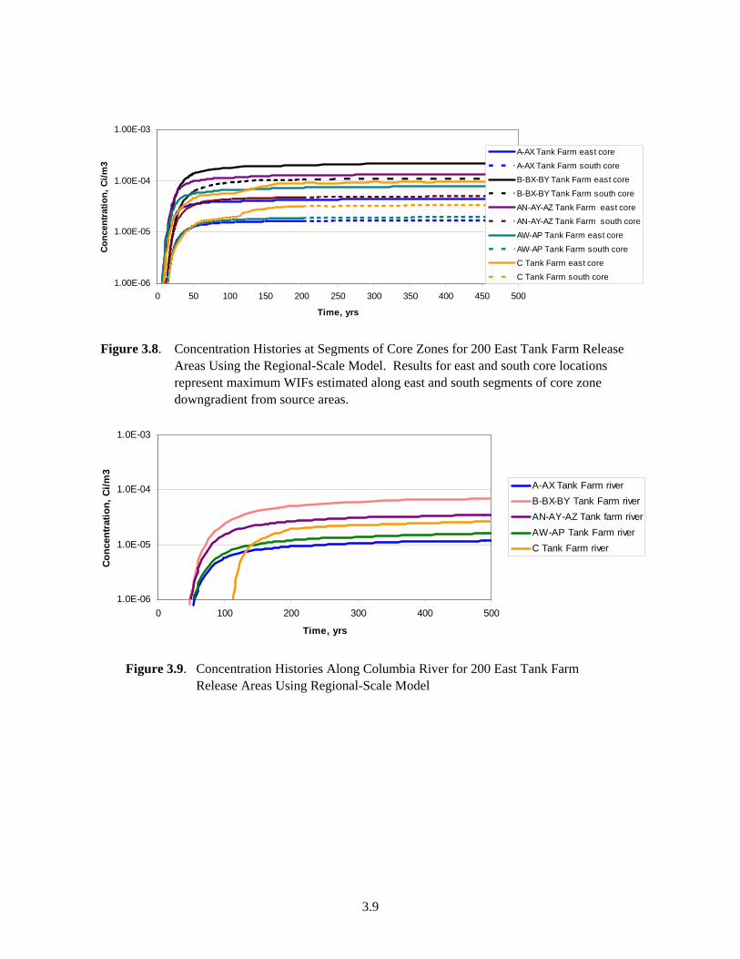
3.2 Tank Farm Area Results Simulations for the tank farms were performed with WIFs only for the regional-scale model described in Section 3. For these simulations, a 1 Ci/m3 concentration source input was applied to an area equal to the assumed tank farm area footprint. Some of the tank farms were grouped together because their collective area could be approximated only with a single node within the grid resolution of the model. Figures 3.6 and 3.7 show the location of the tank farms on the regional grid for the 200 East and West Areas, respectively. The assumed combined tank farm areas in both 200 East and 200 West and the resulting curie loading release, in Ci/yr, are listed in Table 3.4. 3.2.1 200 East Area Tank Farms Figure 3.8 shows concentration histories from releases at the aggregate 200 East Area tank farms at the east and south segments of the core zone. The highest WIFs resulting from these concentration histories occur in the east segment of the core zone for all 200 East tank farms. Figure 3.9 shows the concentration histories from releases at the aggregate 200 East Area tank farms along the Columbia River. WIFs resulting from these concentration histories at the core zone and along the Columbia River are provided in Table 3.5. Results at the core zone location have been subdivided to reflect maximum WIFs estimated along different segments (i.e., north, south, and east segments) of the core zone boundary.

AN-AY-AZ Tanks

A-AX TanksAW-AP Tanks

B-BX-BY TanksC Tanks

Easting (m)

Nor

thin

g(m

)

572000 574000 576000133000

134000

135000

136000

137000

138000

139000

YEAR 949 Figure 3.6. Location of Nodes (denoted in blue) Used to Simulate Contaminant Releases for Aggregated Tank Farms in 200 East Area in Regional-Scale Model Grid

3.8

U Tanks

S-SX-SY Tanks

T-TX-TY Tanks

Easting (m)

Nor

thin

g(m

)

564000 566000 568000133000

134000

135000

136000

137000

138000

139000

Figure 3.7. Location of Nodes (denoted in blue) Used to Simulate Contaminant Releases for Aggregated Tank Farms in 200 West Area in Regional-Scale Model Grid

Table 3.4. Assumed Tank Farm Areas and Annual Curie Loading Used in Regional-Scale Model Simulations (loading rates based on assumed infiltration rate of 5 mm/yr)

Aggregated Tank Farm Area

Assumed Release Areas (m2)

Assumed Curie Loading (Ci/yr)

200 East AN-AY-AZ 28,800 144 A-AX 9,600 48 AW-AP 12,800 64 B-BX-BY 57,600 287.9 C 19,200 96

200 West S-SX 30,400 152 T-TX-TY 35,200 176 U 9,600 48

Modeling results for these releases indicate the plume crosses only the east and south segments of the core zone. Thus, for the 200 East Area tank farms, results for the north segment of the core zone are not included.

3.9

1.00E-06

1.00E-05

1.00E-04

1.00E-03

0 50 100 150 200 250 300 350 400 450 500

Time, yrs

Conc

entra

tion,

Ci/m

3

A-AX Tank Farm east core

A-AX Tank Farm south core

B-BX-BY Tank Farm east core

B-BX-BY Tank Farm south core

AN-AY-AZ Tank Farm east core

AN-AY-AZ Tank Farm south core

AW-AP Tank Farm east core

AW-AP Tank Farm south core

C Tank Farm east core

C Tank Farm south core

Figure 3.8. Concentration Histories at Segments of Core Zones for 200 East Tank Farm Release Areas Using the Regional-Scale Model. Results for east and south core locations represent maximum WIFs estimated along east and south segments of core zone downgradient from source areas.

1.0E-06

1.0E-05

1.0E-04

1.0E-03

0 100 200 300 400 500

Time, yrs

Conc

entr

atio

n, C

i/m3

A-AX Tank Farm riverB-BX-BY Tank Farm riverAN-AY-AZ Tank farm riverAW-AP Tank Farm riverC Tank Farm river

Figure 3.9. Concentration Histories Along Columbia River for 200 East Tank Farm Release Areas Using Regional-Scale Model

3.10

Table 3.5. WIFs at Selected Locations for 200 East Tank Farm Release Areas Using Regional-Scale Model

Recharge Rate (mm/yr) Location 0.1 1.0 4.2 5.0 10.0 50.0

A-AX Tank Farm Area East core(a) 8.85E-07 8.85E-06 3.72E-05 4.43E-05 8.85E-05 4.43E-04 South core(a) 3.53E-07 3.53E-06 1.48E-05 1.77E-05 3.53E-05 1.77E-04 River 2.37E-07 2.37E-06 9.95E-06 1.18E-05 2.37E-05 1.18E-04

AN-AY-AZ Tank Farm Area East core(a) 2.75E-07 2.75E-06 1.16E-05 1.38E-05 2.75E-05 1.38E-04 South core(a) 9.89E-07 9.89E-06 4.15E-05 4.94E-05 9.89E-05 4.94E-04 River 7.03E-07 7.03E-06 2.95E-05 3.51E-05 7.03E-05 3.51E-04

AW-AP Tank Farm Area East core(a) 1.54E-06 1.54E-05 6.47E-05 7.70E-05 1.54E-04 7.70E-04 South core(a) 3.87E-07 3.87E-06 1.62E-05 1.93E-05 3.87E-05 1.93E-04 River 3.87E-07 3.87E-06 1.62E-05 1.93E-05 3.87E-05 1.93E-04

B-BX-BY Tank Farm Area East core(a) 4.42E-06 4.42E-05 1.86E-04 2.21E-04 4.42E-04 2.21E-03 South core(a) 2.24E-06 2.24E-05 9.39E-05 1.12E-04 2.24E-04 1.12E-03 River 1.60E-06 1.60E-05 6.73E-05 8.01E-05 1.60E-04 8.01E-04

C Tank Farm Area East core(a) 1.93E-06 1.93E-05 8.10E-05 9.65E-05 1.93E-04 9.65E-04 South core(a) 6.60E-07 6.60E-06 2.77E-05 3.30E-05 6.60E-05 3.30E-04 River 5.37E-07 5.37E-06 2.25E-05 2.68E-05 5.37E-05 2.68E-04 (a) Results for east and south core locations represent maximum WIFs estimated along east and south segments of the core zone downgradient of the source areas.

Table 3.6 summarizes ratios of release areas for each tank farm relative to the largest assumed area at B-BX-BY tank farm and ratios of associated WIFs relative to the B-BX-BY WIF at the core zone and river for the base-case infiltration of 5 mm/yr. A comparison of WIF ratios with ratios of assumed release areas to the largest release area at the B-BX-BY tank farm shows that the higher the assumed release area, the higher the predicted WIF at any given location. However, at the core zone, the ratios of WIFs do not exactly correspond to the ratios of the assumed areas because of the effect of local-scale groundwater flow regimes and flow paths. At the river, however, the relation of the WIFs at other farms to the B-BX-BY result is nearly identical to those of release areas at the source area. In general, the highest WIF at the east segment of the core zone is calculated for mass releases from the B-BX-BY and AN-AY-AZ tank farms, and the lowest is from the AW-AP tank farm. Based on position alone, one would expect the B-BX-BY tank farm to show the lowest WIF and the AW-AP tank farm to show one of the highest. However, the assumed release area of the B-BX-BY tank farm is about 4.5 times larger than the assumed AW-AP tank farm area, and the B-BX-BY tank farm area is in an area of a relatively higher groundwater flow conditions. This combination of factors affects the calculation of the WIF at this core zone location in this tank farm area.

3.11

Table 3.6. Comparison of Ratios of Assumed Release Area to Largest Release Area in 200 East (B-BX-BY Tank Farm Area) and 200 West (T-TX-TY Tank Farm Area); ratios of WIF to WIFs based on releases in the same areas

Ratio of Assumed Release Area to Release Area Ratio of WIF to WIF from Releases Aggregated

Tank Farm Area Relative to B-BX-BY Tank Farm

200 East East Segment of Core Zone River

A-AX 0.17 0.20 0.15 AN-AY-AZ 0.50 0.06 0.44 AW-AP 0.22 0.35 0.20 B-BX-BY 1.00 1.00 1.00 C 0.33 0.44 0.33 Relative to T-TX-TY Tank Farm

200 West East Segment of Core Zone River

S-SX 0.86 0.86 0.86 T-TX-TY 1.00 1.00 1.00 U 0.27 0.27 0.31

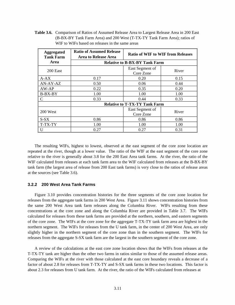
The resulting WIFs, highest to lowest, observed at the east segment of the core zone location are repeated at the river, though at a lower value. The ratio of the WIF at the east segment of the core zone relative to the river is generally about 3.8 for the 200 East Area tank farms. At the river, the ratio of the WIF calculated from releases at each tank farm area to the WIF calculated from releases at the B-BX-BY tank farm (the largest area of release from 200 East tank farms) is very close to the ratios of release areas at the sources (see Table 3.6). 3.2.2 200 West Area Tank Farms Figure 3.10 provides concentration histories for the three segments of the core zone location for releases from the aggregate tank farms in 200 West Area. Figure 3.11 shows concentration histories from the same 200 West Area tank farm releases along the Columbia River. WIFs resulting from these concentrations at the core zone and along the Columbia River are provided in Table 3.7. The WIFs calculated for releases from these tank farms are provided at the northern, southern, and eastern segments of the core zone. The WIFs at the core zone for the aggregate T-TX-TY tank farm area are highest in the northern segment. The WIFs for releases from the U tank farm, in the center of 200 West Area, are only slightly higher in the northern segment of the core zone than in the southern segment. The WIFs for releases from the aggregate S-SX tank farm are the largest in the southern segment of the core zone. A review of the calculations at the east core zone location shows that the WIFs from releases at the T-TX-TY tank are higher than the other two farms in ratios similar to those of the assumed release areas. Comparing the WIFs at the river with those calculated at the east core boundary reveals a decrease of a factor of about 2.8 for releases from T-TX-TY and S-SX tank farms in these two locations. This factor is about 2.3 for releases from U tank farm. At the river, the ratio of the WIFs calculated from releases at

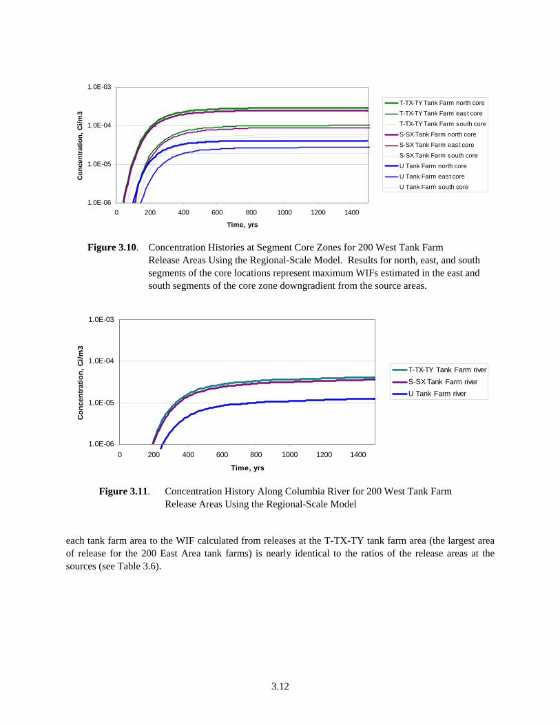
3.12

1.0E-06

1.0E-05

1.0E-04

1.0E-03

0 200 400 600 800 1000 1200 1400

Time, yrs

Conc

entra

tion,

Ci/m

3

T-TX-TY Tank Farm north core

T-TX-TY Tank Farm east core

T-TX-TY Tank Farm south core

S-SX Tank Farm north core

S-SX Tank Farm east core

S-SX Tank Farm south core

U Tank Farm north core

U Tank Farm east core

U Tank Farm south core

Figure 3.10. Concentration Histories at Segment Core Zones for 200 West Tank Farm Release Areas Using the Regional-Scale Model. Results for north, east, and south segments of the core locations represent maximum WIFs estimated in the east and south segments of the core zone downgradient from the source areas.

1.0E-06

1.0E-05

1.0E-04

1.0E-03

0 200 400 600 800 1000 1200 1400

Time, yrs

Con

cent

ratio

n, C

i/m3

T-TX-TY Tank Farm riverS-SX Tank Farm riverU Tank Farm river

Figure 3.11. Concentration History Along Columbia River for 200 West Tank Farm Release Areas Using the Regional-Scale Model

each tank farm area to the WIF calculated from releases at the T-TX-TY tank farm area (the largest area of release for the 200 East Area tank farms) is nearly identical to the ratios of the release areas at the sources (see Table 3.6).

3.13

Table 3.7. WIFs at Selected Locations for 200 West Tank Farm Release Areas Using the Regional-Scale Model

Recharge Rate (mm/yr) Location 0.1 1.0 4.2 5.0 10.0 50.0

S-SX Tank Farm Area East core(a) 1.79E-06 1.79E-05 7.52E-05 8.95E-05 1.79E-04 8.95E-04North core(a) 4.92E-07 4.92E-06 2.07E-05 2.46E-05 4.92E-05 2.46E-04South core(a) 1.02E-06 1.02E-05 4.28E-05 5.10E-05 1.02E-04 5.10E-04River 7.49E-07 7.49E-06 3.14E-05 3.74E-05 7.49E-05 3.74E-04

T-TX-TY Tank Farm Area East core(a) 2.07E-06 2.07E-05 8.71E-05 1.04E-04 2.07E-04 1.04E-03North core(a) 5.69E-06 5.69E-05 2.39E-04 2.85E-04 5.69E-04 2.85E-03South core(a) 1.18E-06 1.18E-05 4.96E-05 5.91E-05 1.18E-04 5.91E-04River 8.67E-07 8.67E-06 3.64E-05 4.34E-05 8.67E-05 4.34E-04

U Tank Farm Area East core(a) 5.68E-07 5.68E-06 2.38E-05 2.84E-05 5.68E-05 2.84E-04North core(a) 8.22E-06 8.22E-05 3.45E-04 4.11E-04 8.22E-04 4.11E-03South core(a) 3.90E-07 3.90E-06 1.64E-05 1.95E-05 3.90E-05 1.95E-04River 2.65E-07 2.65E-06 1.11E-05 1.33E-05 2.65E-05 1.33E-04(a) Results for the north, east, and south core locations represent maximum WIFs estimated along the east and south segments of the core zone downgradient of the source areas.

4.1

4.0 Results Using the Convolution Approach This section summarizes results using the convolution approach for the same source release locations discussed in Section 3. In this approach, the regional-scale model was used to evaluate concentration breakthrough curves from a unit release (1 Ci) over a 10-year period from the IDF and eight aggregate tank farms. Releases from five tank farm areas were evaluated in the 200 East Area, and releases from three aggregate tank farm areas were evaluated in the 200 West Area. Results from all of these releases were evaluated at the core zone and along the Columbia River and are shown in Table 4.1. The breakthrough curves at the east segment of the core zone location and along the river for unit releases from the IDF and aggregate tank farms in the 200 East Area are provided in Figures 4.1 and 4.2. The breakthrough curves at the east segment of the core zone location and along the river are provided in Figures 4.3 and 4.4 for unit releases from the aggregate tank farms in the 200 West Area. As expected, breakthrough curves for release from aggregate tank farms closest to the core zone in the 200 East Area show the earliest arrival times and highest concentrations. The breakthrough curve for releases from the aggregate B-BX-BY tank farms, which are farthest from the core zone, shows the latest peak arrival time and lowest concentration levels. These results reflect the effect of higher-velocity flow regimes directly beneath the B-BX-BY tank farms in the current model. The breakthrough curve for releases from the aggregate A-AX and AW-AP tank farms, which are closest to the core zone, shows the earliest peak arrival times and highest peak concentrations. These results reflect the effect of slightly lower-velocity flow regimes directly beneath these tank farms in the current model.

Table 4.1. Comparison of Unit Release Results at Core Zone and River for IDF and Tank Farm Release Areas with Regional-Scale Model; results for eastern core location represent maximum estimated concentration along east segment of core zone downgradient from source areas (pCi/L)

200 East Area East core(a) Peak (yr) River(b) Peak (yr) IDF Site 16.7 30 1.96 80 A-AX Tank Farm 29.4 22 2.18 85 AN-AY-AZ Tank Farm 29.4 22 1.93 85 AW-AP Tank Farm 31.9 26 1.93 99 B-BX-BY Tank Farm 16.2 32 1.84 95 C Tank Farm 19.2 30 1.66 90

200 West Area S-SX Tank Farm 1.9 280 0.66 380 T-TX-TY Tank Farm 2.4 230 0.58 360 U Tank Farm 2.1 280 0.63 380 (a) Maximum concentration, in pCi/L, over time along the east segment of the core zone. (b) Maximum concentration, in pCi/L, in groundwater over time along the Columbia River.

4.2

0.0

5.0

10.0

15.0

20.0

25.0

30.0

35.0

0 50 100 150 200 250 300 350 400 450 500

Time, yrs

Con

cent

ratio

n, p

Ci/l A-AX

B-BX-BYAN-AY-AZAW-APCIDF

Figure 4.1. Concentration Histories at East Segment of Core Zone for Unit 10-year Release from IDF and Aggregate Tank Farm in 200 East Area Using the Regional-Scale Model. Results for the east core location represents maximum concentration estimated along the east segment of the core zone downgradient from the source areas.

0.0

1.0

2.0

3.0

4.0

5.0

0 50 100 150 200 250 300 350 400 450 500

Time, yrs

Con

cent

ratio

n, p

Ci/l A-AX

B-BX-BYAN-AY-AZAW-APCIDF

Figure 4.2. Concentration Histories Along the Columbia River for a Unit 10-year Release from IDF and Aggregate Tank Farms in 200 East Area Using the Regional-Scale Model

Along the river, the concentration differences between releases from the IDF and tank farm locations are less pronounced, reflecting the dampening effect of the aquifer system and dispersion along flow paths to the river. But the predicted arrival times and concentration levels at the river also show the same general trend—releases from the closest aggregate tank farms exhibit slightly higher concentrations and earlier arrivals.

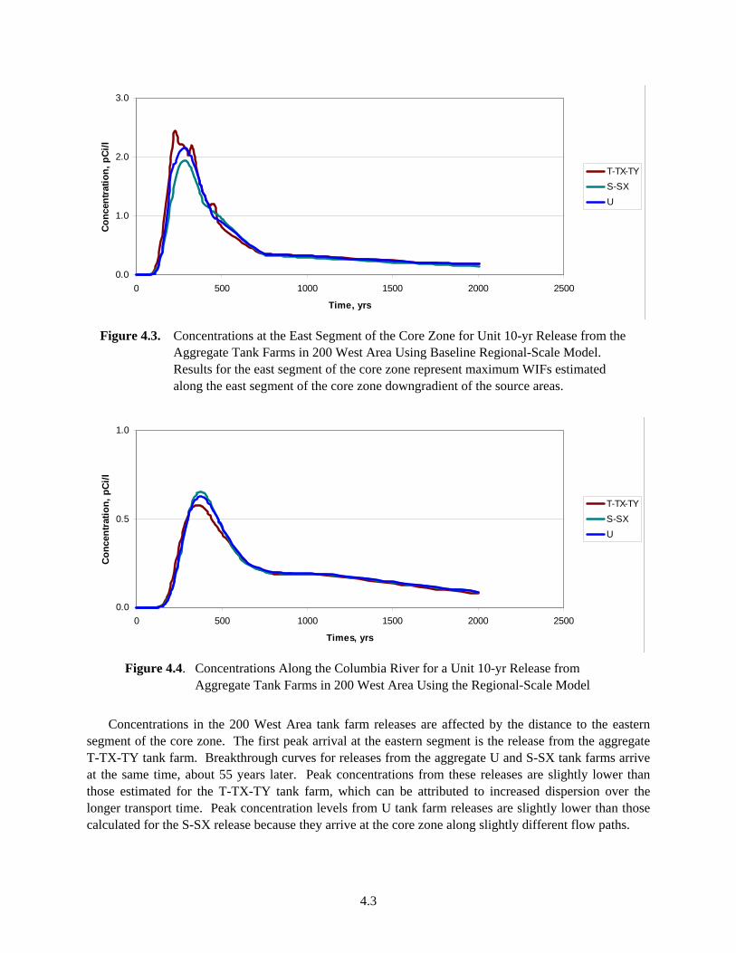
4.3

0.0

1.0

2.0

3.0

0 500 1000 1500 2000 2500

Time, yrs

Conc

entr

atio

n, p

Ci/l

T-TX-TYS-SXU

Figure 4.3. Concentrations at the East Segment of the Core Zone for Unit 10-yr Release from the Aggregate Tank Farms in 200 West Area Using Baseline Regional-Scale Model. Results for the east segment of the core zone represent maximum WIFs estimated along the east segment of the core zone downgradient of the source areas.

0.0

0.5

1.0

0 500 1000 1500 2000 2500

Times, yrs

Con

cent

ratio

n, p

Ci/l

T-TX-TYS-SXU

Figure 4.4. Concentrations Along the Columbia River for a Unit 10-yr Release from Aggregate Tank Farms in 200 West Area Using the Regional-Scale Model

Concentrations in the 200 West Area tank farm releases are affected by the distance to the eastern segment of the core zone. The first peak arrival at the eastern segment is the release from the aggregate T-TX-TY tank farm. Breakthrough curves for releases from the aggregate U and S-SX tank farms arrive at the same time, about 55 years later. Peak concentrations from these releases are slightly lower than those estimated for the T-TX-TY tank farm, which can be attributed to increased dispersion over the longer transport time. Peak concentration levels from U tank farm releases are slightly lower than those calculated for the S-SX release because they arrive at the core zone along slightly different flow paths.

4.4

Like the 200 East Area tank farms, the concentration differences between releases from the different locations are less pronounced once they reach the river. Peak concentrations for releases from the aggregate T-TX-TY and U tank farms are lower than releases from the aggregate S-SX tank farm because part of the plume passes through the gap between Gable Mountain and Gable Butte to the north. The main trajectory of the simulated plume from the aggregate S-SX tank farm area is to the east.

5.1

5.0 Comparison of Alternative Methods The discussion in this section compares the results from the alternative approaches for two example mass-release scenarios: 1) a long-term increasing contaminant release from glassified low-level wastes disposed in 200 East Area and 2) a shorter-term hypothetical mass release from a tank farm in 200 West Area. The long-term contaminant release example was adapted from work by Mann et al. (2001) for a 10,000-yr base case involving a source release from ILAW disposed of as a glass waste form at the IDF in 200 East Area. This analysis evaluated a source release from the glass wastes with an assumed technetium-99 inventory of 25,550 Ci. The shorter-term release example was derived from a hypothetical release postulated for a tank waste retrieval scenario at the S-SX tank farm in the 200 West Area in the tank farm closure analysis. This scenario was one of several cases evaluated by Zhang et al. (2004) as a part of that analysis. This specific case involved a source release of an assumed technetium-99 inventory of 0.7 Ci over 600 years. Results of the two calculations are also compared with results from a direct simulation approach.

5.1 Long-Term Increasing Release Scenario Predicted concentrations at the core zone boundary and along the Columbia River using direct numerical simulation were established for the long-term contaminant release case described above to facilitate comparison of results from the WIF approach with results using the convolution approach. This simulation was based on a steady-state flow field calculated with the regional flow model. The specific annual release rate used in the simulation is shown in Figure 5.1. The annual release rate is 5.75E-11 Ci/yr at the start of the simulation, increasing to 1.68E-02 Ci/yr at 10,000 years. The overall cumulative release during the 10,000 years of interest was about 84 Ci. Concentration breakthrough curves from this simulation for the east segment of the core zone and the Columbia River are provided in Figure 5.2. The peak concentration established at the end of 10,000 years was 12 pCi/L in the eastern segment of the core zone and 6.5 pCi/L at the river. The calculated breakthrough curves at the core zone and along the river, while different in magnitude, are similar in shape and reflect the nature of the increasing contaminant release rate introduced into the model during the course of the simulation (Figure 5.1). Figure 5.3 compares predicted technetium-99 concentrations in the eastern segment of the core zone and along the Columbia River from direct simulation with predictions from the WIF and convolution approaches. In this specific long-term release case, all three methods produce breakthrough curves at any location downgradient from the source area that are similar in shape to the long-term release curves used in the simulation. Results at the core zone and along the river using the convolution approach were very similar to those developed with direct simulation at comparable locations. Predictions using the convolution approach were about 4 percent higher and 10 percent lower at the core zone and along the river, respectively, than direct simulation predictions.

5.2

Time, yrs

Sou

rce

Are

aR

elea

se,C

i

0 2500 5000 7500 1000010-3

10-2

10-1

100

101

102

Cummulative Release (Ci)Annual Release (Ci/yr)

Figure 5.1. Annual and Cumulative Long-Term Contaminant Release Example—a Source

Release from ILAW Glass Wastes Containing 25,550 Ci of 99Tc near the IDF (adapted from Mann et al. 2001). The overall cumulative release during the10,000 years of interest was about 84 Ci.

T im e , yrs

Con

cent

ratio

n,pC

i/L

2 5 0 0 5 0 0 0 7 5 0 0 1 0 0 0 00

1

2

3

4

5

6

7

8

9

1 0

1 1

1 2

1 3

1 4

E a st C o re Z o n eA lo n g R ive r

Figure 5.2. Predicted 99Tc Concentrations at East Segment of Core Zone and Along the

Columbia River by Direct Simulation of Long-Term Source Release from ILAW Glass Wastes Containing 25,550 Ci of 99Tc near the IDF (adapted from Mann et al. 2001). The overall cumulative release during the 10,000 years of interest was about 84 Ci.

5.3

East Segment of Core Zone

1.E-01

1.E+00

1.E+01

1.E+02

0 2000 4000 6000 8000 10000

Time, yrs

Conc

entra

tion,

pCi

/l

Direct SimulationWIFConvolution

Along the Columbia River

1.E-01

1.E+00

1.E+01

1.E+02

0 2000 4000 6000 8000 10000

Time, yrs

Conc

entra

tion,

pCi

/l

Direct SimulationWIFConvolution

Figure 5.3. Comparison of Predicted 99Tc Concentrations Using Direct Simulation with the WIF

and Convolution Approaches at the Eastern Segment of the Core Zone and Along the Columbia River. Results are for a long-term source release from ILAW glass wastes containing 5,550 Ci of 99Tc at the IDF (adapted from Mann et al. 2001). The overall cumulative release during the10,000 years of interest was about 84 Ci.

5.4

The comparison also showed that results developed with the WIF approach were similar to the convolution and direct simulated approaches at comparable locations. WIF results were quite similar to direct simulation results at the core zone and along the river (see Figure 5.3 and Table 5.1). Core zone results were within 10 percent (higher) of those from direct simulation, and results along the river were within 11 percent (lower) of comparable direct simulation results.

Table 5.1. Comparison of Predicted Peak 99Tc Concentrations Using Direct Simulation with WIF and Convolution Approaches at the East Segment of the Core Zone and Along Columbia River. Results are for a long-term source release from ILAW glass wastes containing 25,550 Ci of 99Tc at the IDF (adapted from Mann et al. 2001).

Estimation Methods

Direct Simulation Well Intercept Factor Convolution Location

99Tc Concentration (pCi/L) East Segment of the Core Zone 12.1 13.3 12.6

Along the River 6.5 5.8 5.8

5.2 Shorter-Term Release Scenario A predicted set of concentrations at the core zone boundary and along the Columbia River using direct numerical simulation was established for the example shorter-term contaminant release case. This hypothetical tank leak from the S-SX tank farm area evaluated in Zhang et al. (2004) was used to facilitate comparisons of the alternative approaches. This simulation, which is described more fully in Zhang et al. (2004), was based on a steady-state flow field calculated with the regional flow model and based on the annual release rates shown in Figure 5.4. The annual release rate starts at 1.0E-14 Ci/yr and increases to a peak of 5.0E-03 Ci/yr before declining to a rate of 8.0E-05 at 600 years. Overall cumulative release after 600 years of simulation was about 0.7 Ci. Concentration breakthrough curves for the east segment of the core zone location and Columbia River resulting from direct simulation of the shorter-term release case are provided in Figure 5.5. The peak 99Tc concentration established with direct simulation during the 600 years was about 3 pCi/L along the eastern segment of the core zone and about 1 pCi/L along the river. The calculated breakthrough curves at the core zone and along the river, while different magnitudes, are similar in shape and different from the relatively short-duration release curve used in the simulation (Figure 5.4). Because of dispersion, the rounding and flattening of the input source release curve was expected as it is introduced into the aquifer and transported over several kilometers before reaching the east segment and the river.

5.5

0.00001

0.0001

0.001

0.01

0.1

1

0 100 200 300 400 500 600

Time, yrs

Rele

ase,

Ci

AnnualCumulative

Figure 5.4. Annual and Cumulative Shorter-Term Contaminant Release Example. Results are from

600-yr release of ~0.7 Ci of 99Tc from S-SX tank farm (adapted from Zhang et al. (2004)

1.0E-03

1.0E-02

1.0E-01

1.0E+00

1.0E+01

1.0E+02

1.0E+03

1.0E+04

1.0E+05

1.0E+06

0 100 200 300 400 500 600

Time, yrs

Con

cent

ratio

n (p

Ci/l

)

Source250 m (Direct. Sim.)250 m (WIF)250 m (Convolution)Core Zone (Direct. Sim.)Core Zone (WIF)Core Zone (Convolution)Along River (Direct. Sim.)Along River (WIF)Along River (Convolution)

Figure 5.5. Comparison of Predicted 99Tc Concentrations Using Direct Simulation with the WIF and

Convolution Approaches at Eastern Segment of Core Zone and Along the Columbia River. Results are from 600-yr release of ~0.7 Ci of 99Tc from S-SX Tank Farm (adapted from Zhang et al. 2004).

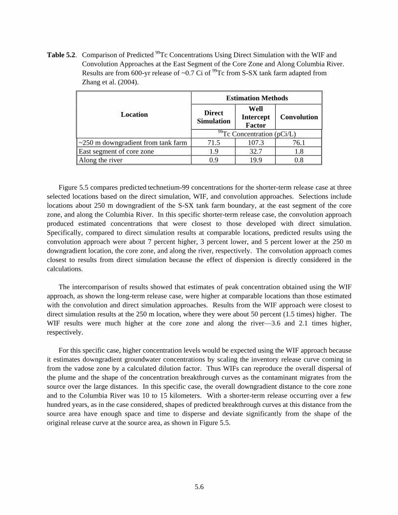
5.6

Table 5.2. Comparison of Predicted 99Tc Concentrations Using Direct Simulation with the WIF and Convolution Approaches at the East Segment of the Core Zone and Along Columbia River. Results are from 600-yr release of ~0.7 Ci of 99Tc from S-SX tank farm adapted from Zhang et al. (2004).

Estimation Methods

Direct Simulation

Well Intercept

Factor Convolution Location

99Tc Concentration (pCi/L) ~250 m downgradient from tank farm 71.5 107.3 76.1 East segment of core zone 1.9 32.7 1.8 Along the river 0.9 19.9 0.8

Figure 5.5 compares predicted technetium-99 concentrations for the shorter-term release case at three selected locations based on the direct simulation, WIF, and convolution approaches. Selections include locations about 250 m downgradient of the S-SX tank farm boundary, at the east segment of the core zone, and along the Columbia River. In this specific shorter-term release case, the convolution approach produced estimated concentrations that were closest to those developed with direct simulation. Specifically, compared to direct simulation results at comparable locations, predicted results using the convolution approach were about 7 percent higher, 3 percent lower, and 5 percent lower at the 250 m downgradient location, the core zone, and along the river, respectively. The convolution approach comes closest to results from direct simulation because the effect of dispersion is directly considered in the calculations. The intercomparison of results showed that estimates of peak concentration obtained using the WIF approach, as shown the long-term release case, were higher at comparable locations than those estimated with the convolution and direct simulation approaches. Results from the WIF approach were closest to direct simulation results at the 250 m location, where they were about 50 percent (1.5 times) higher. The WIF results were much higher at the core zone and along the river—3.6 and 2.1 times higher, respectively. For this specific case, higher concentration levels would be expected using the WIF approach because it estimates downgradient groundwater concentrations by scaling the inventory release curve coming in from the vadose zone by a calculated dilution factor. Thus WIFs can reproduce the overall dispersal of the plume and the shape of the concentration breakthrough curves as the contaminant migrates from the source over the large distances. In this specific case, the overall downgradient distance to the core zone and to the Columbia River was 10 to 15 kilometers. With a shorter-term release occurring over a few hundred years, as in the case considered, shapes of predicted breakthrough curves at this distance from the source area have enough space and time to disperse and deviate significantly from the shape of the original release curve at the source area, as shown in Figure 5.5.

6.1

6.0 Summary and Conclusions Alternatives to direct numerical simulation of contaminant transport and dispersion are available and useful for assessments that need to estimate groundwater concentrations migrating from future vadose zone mass to the unconfined aquifer. These methods can be appropriate for estimating groundwater concentrations from vadose zone releases if:

mass release reaches the unconfined aquifer after the effects of current transient changes to the vadose zone and aquifer system have dissipated

flow conditions in the unconfined aquifer can be assumed to be at steady-state. Comparisons of results using the WIF and convolution approaches with results from direct simulation for two contrasting cases yield the following conclusions: For the long-term contaminant release scenario case (a source release from ILAW glass wastes containing 25,550 Ci of technetium-99 near the IDF) (adapted from Mann et al. 2001), the convolution approach estimated concentrations that were closest to those developed with direct simulation. Results at the core zone and along the river using the convolution approach were very similar to results at comparable locations developed with direct simulation. Predictions using the convolution approach were about 4 percent higher and 10 percent lower than direct simulation at the core zone and along the river, respectively. The comparison also showed that results developed with the WIF approach were similar to those estimated with the convolution and direct simulation approaches at comparable locations. The WIF predictions at the core zone and along the river were within 10 percent (higher) and 11 percent (lower), respectively, of direct simulation. For the shorter-term contaminant release scenario (a hypothetical 600-yr release of ~0.7 Ci of technetium-99 from the S-SX tank farm area) (adapted from Zhang et al. 2004), the convolution approach estimated concentrations that were closest to those developed with direct simulation. Specifically, when compared to direct simulation results at comparable locations, predictions from the convolution approach were about 7 percent higher, 3 percent lower, and 5 percent lower at the 250 m downgradient location, core zone, and along the river, respectively. The convolution results are closest to estimates from direct simulation because the effect of dispersion is directly considered in the calculations. The intercomparison of results from the WIF approach, as shown in the long-term release case, produced higher peak concentrations than those estimated with the convolution and direct simulation approaches at comparable locations. Compared with direct simulation, results from the WIF approach were closest to direct simulation results at the 250 m location—where they were about 1.5 times higher. The WIF results were much higher at the core zone and along the river—about 17 and 22 times higher, respectively. This analysis concludes that because estimating peak concentrations with the WIF approach basically involves scaling the time series of input source concentrations from the vadose zone to the aquifer by the calculated WIFs, results would be reasonably accurate for estimating groundwater concentrations near the

6.2

source release. However, the convolution approach would more closely approximate groundwater concentrations at locations farther from the source area. For the two cases considered, the WIF approach overestimates peak concentrations away from the source area. The WIF method overestimates predicted peak concentrations at downgradient locations as the breakthrough curves deviate from the shape of the input function in response to plume dispersion. Results are generally influenced by two factors: the duration of the source term release to the water table and the downgradient distance to points of calculations. Comparison of WIF results with direct simulation results for the two cases evaluated provided a general measure of the overall magnitude of the deviation that could be expected for IDF and tank farm locations. Peak concentrations estimated with the WIF approach would tend to be closer to results from direct simulation for longer-term releases of contaminants where the shapes of breakthrough curves at various points of calculations are similar to the original release curve introduced in the source area. For the ILAW glass release case evaluated at the IDF in 200 East Area, WIF results at the core zone and along the river were within 10 percent (higher) and 11 percent (lower), respectively, of comparable direct simulation results. The overestimation of peak concentrations with the WIF approach tends to be higher for shorter-term releases of contaminants where breakthrough curve shapes at various points of calculations are influenced by plume dispersion and deviate from the original release curve introduced in the source area. For the hypothetical tank leak case evaluated at the S-SX Tank Farm in the 200 West Area, where the points of calculations are considerably farther away from the source area, WIF results at the core zone and along the river were on the order of 17 and 22 times higher than comparable direct simulation results.

7.1

7.0 References Bergeron MP and SK Wurstner. 2000. Groundwater Flow and Transport Calculations Supporting the Immobilized Low-Activity Waste Disposal Facility Performance Assessment. PNNL-13400, Pacific Northwest National Laboratory, Richland, Washington.

Bryce RW, CT Kincaid, PW Eslinger, and LF Morasch (eds.). 2002. An Initial Assessment of Hanford Impact Performed with the System Assessment Capability. PNNL-14027, Pacific Northwest National Laboratory, Richland, Washington.

Cole CR, SK Wurstner, MP Bergeron, MD Williams, and PD Thorne. 1997. Three-Dimensional Analysis of Future Groundwater Flow Conditions and Contaminant Plume Transport in the Hanford Site Unconfined Aquifer System: FY 1996 and 1997 Status Report. PNNL-11801, Pacific Northwest National Laboratory, Richland, Washington.

Cole CR, MP Bergeron, SK Wurstner, PD Thorne, S Orr, and MI McKinley. 2001a. Transient Inverse Calibration of the Site-Wide Groundwater Flow Model to Hanford Operational Impacts from 1943 to 1996. PNNL-13447, Pacific Northwest National Laboratory, Richland, Washington.

Cole CR, MP Bergeron, CJ Murray, PD Thorne, SK Wurstner, and PM Rogers. 2001b. Uncertainty Analysis Framework—Hanford Site-Wide Groundwater Flow and Transport Model. PNNL-13641, Pacific Northwest National Laboratory, Richland, Washington.

DOE/RL. 2004. Final Hanford Site Solid (Radioactive and Hazardous) Waste Program Environmental Impact Statement, Richland, Washington. DOE/EIS-0286F, U.S. Department of Energy Richland Operations Office, Richland, Washington.

Freeze RA and JA Cherry. 1979. Groundwater. Prentice-Hall, Inc., Englewood Cliffs, New Jersey.

Gupta SK, CR Cole, CT Kincaid, and AM Monti. 1987. Coupled Fluid, Energy, and Solute Transport (CFEST) Model: Formulation and User’s Manual. BMI/ONWI-660, Battelle Memorial Institute, Office of Nuclear Waste Isolation, Columbus, Ohio.

Hartman MJ, editor. 2000. Hanford Site Groundwater Monitoring: Setting, Sources, and Methods. PNNL-13080, Pacific Northwest National Laboratory, Richland, Washington.

Kincaid CT, MP Bergeron, CR Cole, MD Freshley, NL Hassig, VG Johnson, DI Kaplan, RJ Serne, GP Streile, DL Strenge, PD Thorne, LW Vail, GA Whyatt, and SK Wurstner. 1998. Composite Analysis for Low-Level Waste Disposal in the 200-Area Plateau of the Hanford Site. PNNL-11800, Pacific Northwest National Laboratory, Richland, Washington.

Lee T. 1999. Applied Mathematics in Hydrogeology. Lewis Publishers, Boca Raton, Florida.

Lindsey KA. 1995. Miocene- to Pliocene-Aged Suprabasalt Sediments of the Hanford Site, South-Central Washington. BHI-00184 Rev 00, Bechtel Hanford Inc., Richland, Washington.

Mann FM, CR Eiholzer, R Khaleel, NW Kline, AH Lu, BP McGrail, PD Rittmann, and F Schmittroth. 1995. Definition of the Base Analysis Case of the Interim Performance Assessment. WHC-SD-WM-RPT-200 Rev. 0, Westinghouse Hanford Company, Richland, Washington.

7.2

Mann FM. 1996. INTEG: A Program to Calculate Groundwater Contamination and Human Doses. WHC-SD-WM-RPT-219, Westinghouse Hanford Company, Richland, Washington.

Mann FM, KC Burgard, WR Root, RJ Puigh, SH Finfrock, R Khaleel, DH Bacon, EJ Freeman, BP McGrail, MP, Bergeron, SK Wurstner, and PE LaMont. 2001. Hanford Immobilized Low-Activity Waste Performance Assessment: 2001 Version. DOE/ORP-2000-24 Rev. 0, U.S. Department of Energy Office of River Protection, Richland, Washington.

Mann FM, RJ Puigh, SH Finfrock, R Khaleel and MI Wood. 2003a. Integrated Disposal Facility Risk Assessment. RPP-15834, CH2M HILL Hanford Group, Inc., Richland, Washington.

Mann FM, BP McGrail, DH Bacon, RJ Serne, KM Krupka, RJ Puigh, R Khaleel, and SH Finfrock. 2003b. Risk Assessment Supporting the Decision on the Initial Selection of Supplemental ILAW Technologies. RPP-17675, CH2M HILL Hanford Group, Inc., Richland, Washington.

Mills DB, DB Porcella, MJ Ungs, SA Gherini, KV Summers, Lingfung Mok, GL Rupp, GL Bowie, and DA Haith. 1985. Water Quality Assessment: A Screening Procedure for Toxic and Conventional Pollutants, Part II. EPA/600/6-85/002b, Environmental Research Laboratory Office of Research and Development, U.S. Environmental Protection Agency, Athens, Georgia.

Nichols WE, NJ Aimo, M Oostrom, and MD White. 1997. STOMP Subsurface Transport Over Multiple Phases: Application Guide. PNNL-11216, Pacific Northwest National Laboratory, Richland, Washington.

Rawlins JA, RA Karnesky, R Khaleel, AH Lu, FM Mann, BP McGrail, WJ McMahon, MG Piepho, PD Rittmann, and F Schmittroth. 1994. Impacts of Disposal System Design Options on Low-Level Glass Waste Disposal System Performance. WHC-EP-0810 Rev. 0, Westinghouse Hanford Company, Richland, Washington.

Rittmann PD. 1993. GRTPA - A Program to Calculate Human Dose from PORFLOW Output. WHC-SD-WM-UM-018, Westinghouse Hanford Company, Richland, Washington.

Thorne PD, MA Chamness, FA Spane Jr, VR Vermeul, and WD Webber. 1993. Three-Dimensional Conceptual Model for the Hanford Site Unconfined Aquifer System, FY 1993 Status Report. PNL-8971, Pacific Northwest Laboratory, Richland, Washington.

Walters WH, MC Richmond, and BG Gilmore. 1994. Reconstruction of Radionuclide Concentrations in the Columbia River from Hanford, Washington to Portland Oregon, January 1950–January 1971. PNWD-2225 HEDR, Battelle Pacific Northwest Laboratories, Richland, Washington.

Walton WC. 1985. Practical Aspects of Groundwater Modeling: Flow, Mass and Heat Transport, and Subsidence, Analytical and Computer Models, Second Edition. National Water Well Association, Worthington, Ohio.

White MD and M Oostrom. 1996. STOMP Subsurface Transport Over Multiple Phases: Theory Guide. PNNL-11217, Pacific Northwest National Laboratory, Richland, Washington.

White MD and M Oostrom. 1997. STOMP Subsurface Transport Over Multiple Phases: User’s Guide. PNNL-11218, Pacific Northwest National Laboratory, Richland, Washington.

7.3

Wurstner SK, PD Thorne, MA Chamness, MD Freshley, and MD Williams. 1995. Development of a Three-Dimensional Groundwater Model of the Hanford Site Unconfined Aquifer System: FY 1995 Status Report. PNL-10886, Pacific Northwest Laboratory, Richland, Washington.

Zhang ZF, VL Freedman, SR Waichler, and MD White. 2004. 2004 Initial Assessments of Closure for the S-SX Tank Farm: Numerical Simulations. PNNL-14604, Pacific Northwest National Laboratory, Richland, Washington.

PNNL-14891

Distr.1

Distribution

No. of Copies DOE Office of River Protection P. E. Lamont* R. W. Lober* S. Wiegman* 5 DOE Richland Operations Office R. D. Hildebrand (5) A6-38 J. G. Morse* K. M. Thompson* CH2M HILL Hanford Group, Inc. F. J. Anderson* M. P. Connelly* A. J. Knepp* F. M. Mann* W. J. McMahon* D. A. Myers* Fluor Federal Services R. Khaleel* R. J. Puigh*

No. of Copies Fluor Hanford, Inc. T. W. Fogwell* M. I. Wood* 10 Pacific Northwest National Laboratory M. P. Bergeron (5) K9-36 R. W. Bryce* C. R. Cole* M. J. Fayer* E. J. Freeman (3) K9-36 V. Freedman* M. D. Freshley* C. T. Kincaid* G. V. Last* W. E. Nichols* S. P. Reidel* P. D. Thorne* M. B. Triplett* M. D. Williams* S. K. Wurstner* Hanford Technical Library (2) P8-55 * Electronic Notification Only